Overview. Apriori Algorithm Support is 50% (2/4) Confidence is 66.67% (2/3) TX1Shoes,Socks,Tie...
57
Overview
-
Upload
audra-haynes -
Category
Documents
-
view
226 -
download
2
Transcript of Overview. Apriori Algorithm Support is 50% (2/4) Confidence is 66.67% (2/3) TX1Shoes,Socks,Tie...

Overview

Apriori Algorithm
Support is 50% (2/4) Confidence is 66.67% (2/3)
TX1 Shoes,Socks,Tie
TX2 Shoes,Socks,Tie,Belt,Shirt
TX3 Shoes,Tie
TX4 Shoes,Socks,Belt
€
Socks⇒ Tie
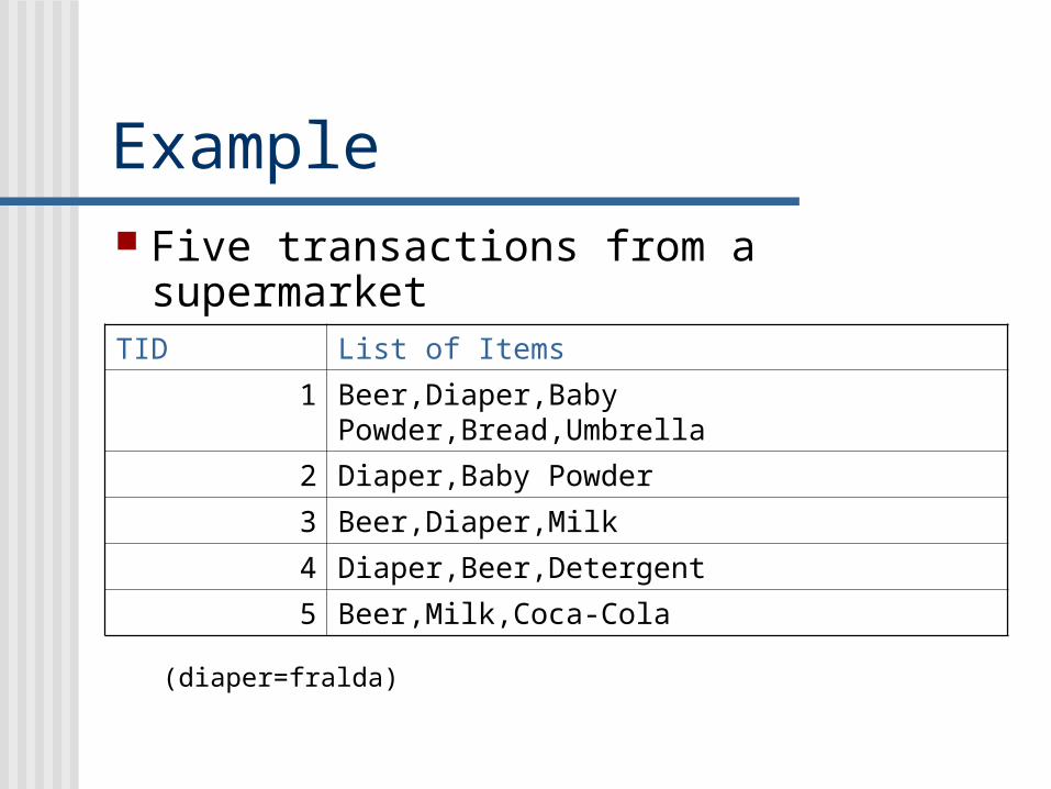
Example Five transactions from a supermarket
(diaper=fralda)
TID List of Items
1 Beer,Diaper,Baby Powder,Bread,Umbrella
2 Diaper,Baby Powder
3 Beer,Diaper,Milk
4 Diaper,Beer,Detergent
5 Beer,Milk,Coca-Cola
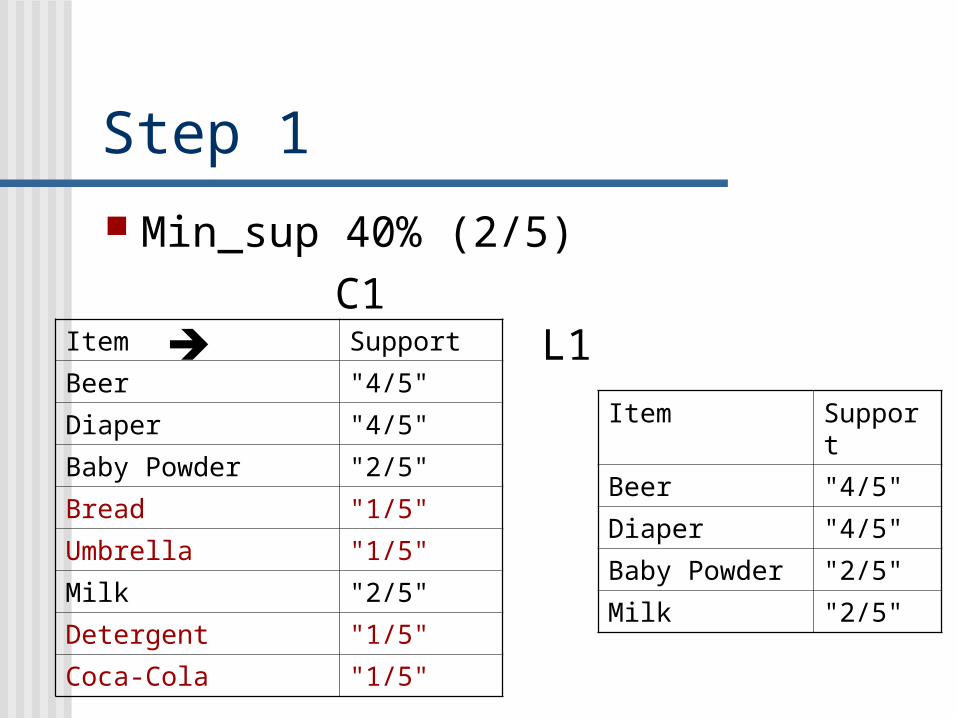
Step 1
Min_sup 40% (2/5)
C1 L1Item Support
Beer "4/5"
Diaper "4/5"
Baby Powder "2/5"
Bread "1/5"
Umbrella "1/5"
Milk "2/5"
Detergent "1/5"
Coca-Cola "1/5"
Item Support
Beer "4/5"
Diaper "4/5"
Baby Powder "2/5"
Milk "2/5"
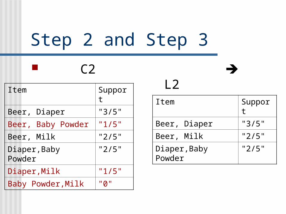
Step 2 and Step 3
C2 L2
Item Support
Beer, Diaper "3/5"
Beer, Baby Powder "1/5"
Beer, Milk "2/5"
Diaper,Baby Powder "2/5"
Diaper,Milk "1/5"
Baby Powder,Milk "0"
Item Support
Beer, Diaper "3/5"
Beer, Milk "2/5"
Diaper,Baby Powder
"2/5"
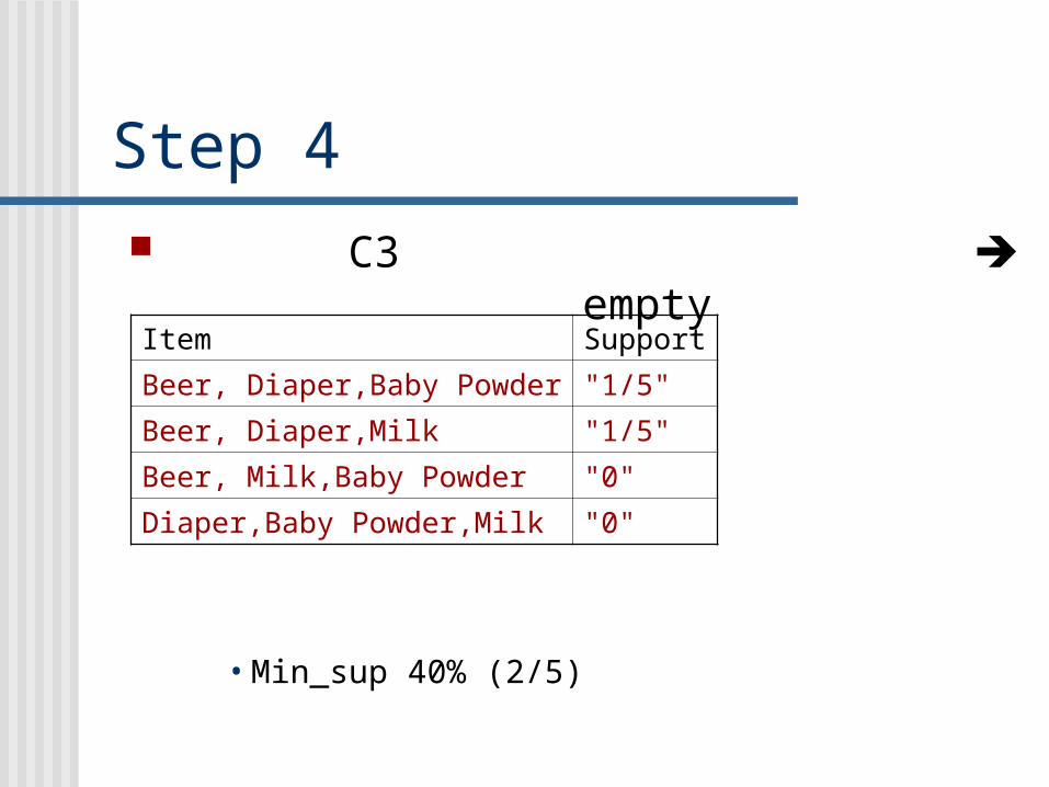
Step 4
C3 empty
• Min_sup 40% (2/5)
Item Support
Beer, Diaper,Baby Powder "1/5"
Beer, Diaper,Milk "1/5"
Beer, Milk,Baby Powder "0"
Diaper,Baby Powder,Milk "0"
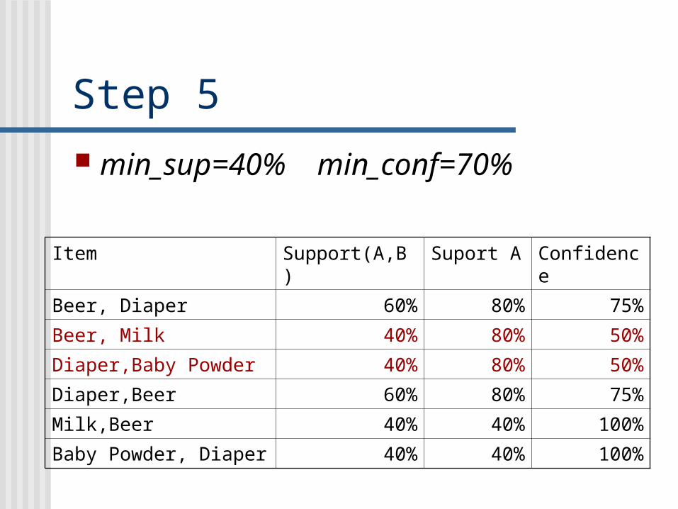
Step 5
min_sup=40% min_conf=70%
Item Support(A,B) Suport A Confidence
Beer, Diaper 60% 80% 75%
Beer, Milk 40% 80% 50%
Diaper,Baby Powder 40% 80% 50%
Diaper,Beer 60% 80% 75%
Milk,Beer 40% 40% 100%
Baby Powder, Diaper 40% 40% 100%
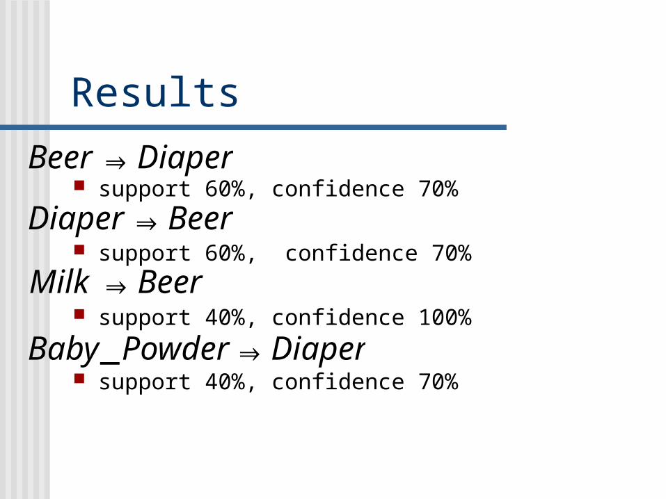
Results
support 60%, confidence 70%
support 60%, confidence 70%
support 40%, confidence 100%
support 40%, confidence 70%
€
Beer ⇒ Diaper
€
Diaper ⇒ Beer
€
Milk ⇒ Beer
€
Baby _ Powder ⇒ Diaper
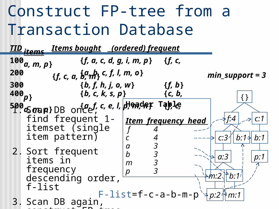
Construct FP-tree from a Transaction Database
{}
f:4 c:1
b:1
p:1
b:1c:3
a:3
b:1m:2
p:2 m:1
Header Table
Item frequency head f 4c 4a 3b 3m 3p 3
min_support = 3
TID Items bought (ordered) frequent items100 {f, a, c, d, g, i, m, p} {f, c, a, m, p}200 {a, b, c, f, l, m, o} {f, c, a, b, m}300 {b, f, h, j, o, w} {f, b}400 {b, c, k, s, p} {c, b, p}500 {a, f, c, e, l, p, m, n} {f, c, a, m, p}
1. Scan DB once, find frequent 1-itemset (single item pattern)
2. Sort frequent items in frequency descending order, f-list
3. Scan DB again, construct FP-tree F-list=f-c-a-b-m-p
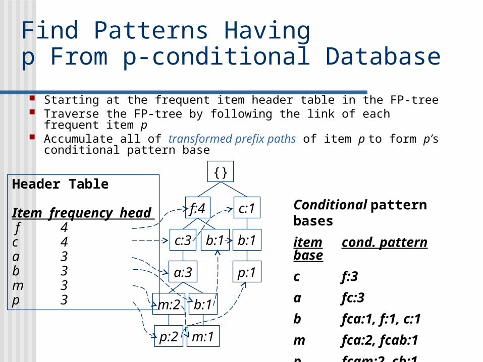
Find Patterns Having p From p-conditional Database
Starting at the frequent item header table in the FP-tree Traverse the FP-tree by following the link of each frequent item p Accumulate all of transformed prefix paths of item p to form p’s
conditional pattern base
Conditional pattern bases
item cond. pattern base
c f:3
a fc:3
b fca:1, f:1, c:1
m fca:2, fcab:1
p fcam:2, cb:1
{}
f:4 c:1
b:1
p:1
b:1c:3
a:3
b:1m:2
p:2 m:1
Header Table
Item frequency head f 4c 4a 3b 3m 3p 3
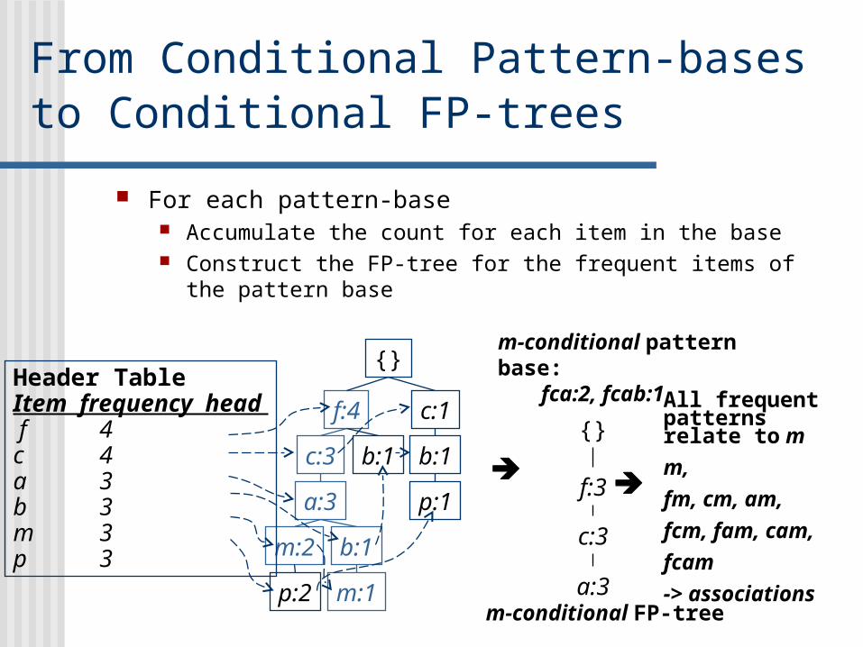
From Conditional Pattern-bases to Conditional FP-trees
For each pattern-base Accumulate the count for each item in the base Construct the FP-tree for the frequent items of the pattern base
m-conditional pattern base:fca:2, fcab:1
{}
f:3
c:3
a:3m-conditional FP-tree
All frequent patterns relate to m
m,
fm, cm, am,
fcm, fam, cam,
fcam
-> associations
{}
f:4 c:1
b:1
p:1
b:1c:3
a:3
b:1m:2
p:2 m:1
Header TableItem frequency head f 4c 4a 3b 3m 3p 3

The Data Warehouse Toolkit, Ralph Kimball, Margy Ross, 2nd ed, 2002
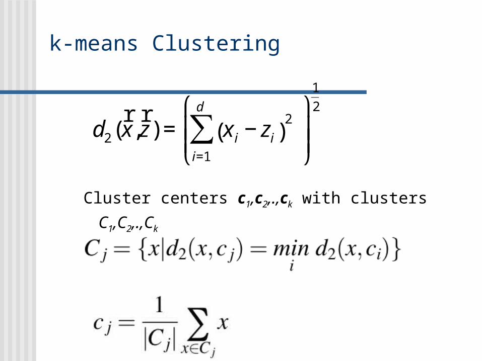
k-means Clustering
Cluster centers c1,c2,.,ck with clusters C1,C2,.,Ck
€
d2(r x ,
r z ) = x i − zi( )
2
i=1
d
∑ ⎛
⎝ ⎜ ⎜
⎞
⎠ ⎟ ⎟
1
2
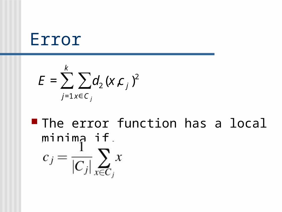
Error
The error function has a local minima if,
€
E = d2(x,c j )2
x∈C j
∑j=1
k
∑
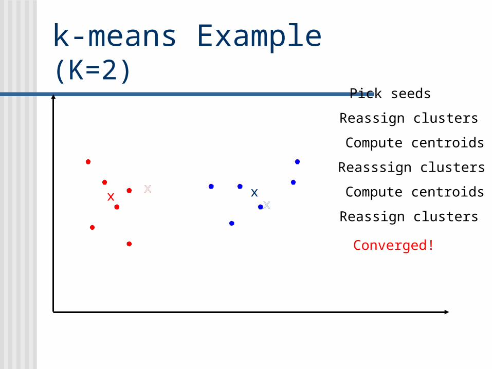
k-means Example(K=2)
Pick seeds
Reassign clusters
Compute centroids
xx
Reasssign clusters
xx xx Compute centroids
Reassign clusters
Converged!
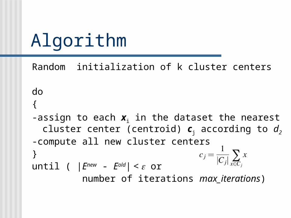
AlgorithmRandom initialization of k cluster centers
do{
-assign to each xi in the dataset the nearest cluster center (centroid) cj according to d2
-compute all new cluster centers }until ( |Enew - Eold| < or number of iterations max_iterations)
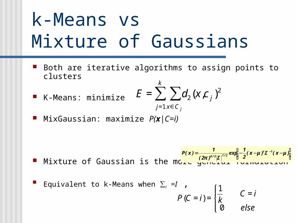
k-Means vs Mixture of Gaussians Both are iterative algorithms to assign points to clusters
K-Means: minimize
MixGaussian: maximize P(x|C=i)
Mixture of Gaussian is the more general formulation
Equivalent to k-Means when ∑i =I ,
⎥⎦
⎤⎢⎣
⎡ −−−= − )x()x(2
1exp
)2(
1)x(P 1t
2/12/dμΣμ
Σπ
€
P(C = i) =1
kC = i
0 else
⎧ ⎨ ⎪
⎩ ⎪
€
E = d2(x,c j )2
x∈C j
∑j=1
k
∑
Tree Clustering Tree clustering algorithm allow us to
reveal the internal similarities of a given pattern set
To structure these similarities hierarchically
Applied to a small set of typical patterns For n patterns these algorithm generates
a sequence of 1 to n clusters
Example
Similarity between two clusters is assessed by measuring the similarity of the furthest pair of patterns (each one from the distinct cluster)
This is the so-called complete linkage rule
Zur Anzeige wird der QuickTime™ Dekompressor „TIFF (LZW)“
benötigt.
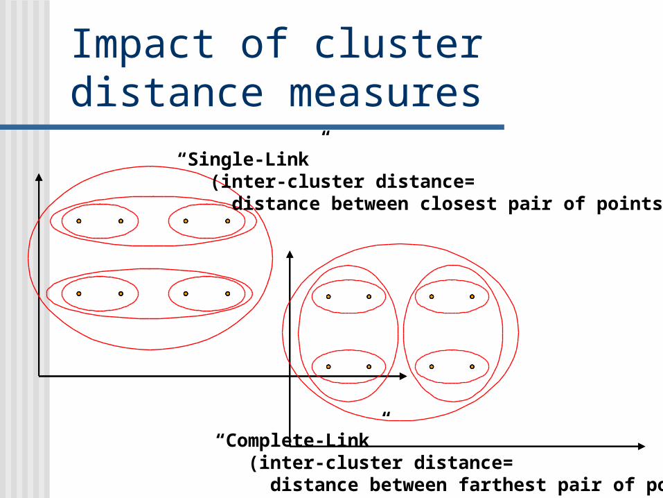
Impact of cluster distance measures
“Single-Link” (inter-cluster distance= distance between closest pair of points)
“Complete-Link” (inter-cluster distance= distance between farthest pair of points)

There are two criteria proposed for clustering evaluation and selection of an optimal clustering scheme (Berry and Linoff, 1996)
Compactness, the members of each cluster should be as close to each other as possible. A common measure of compactness is the variance, which should be minimized
Separation, the clusters themselves should be widely spaced
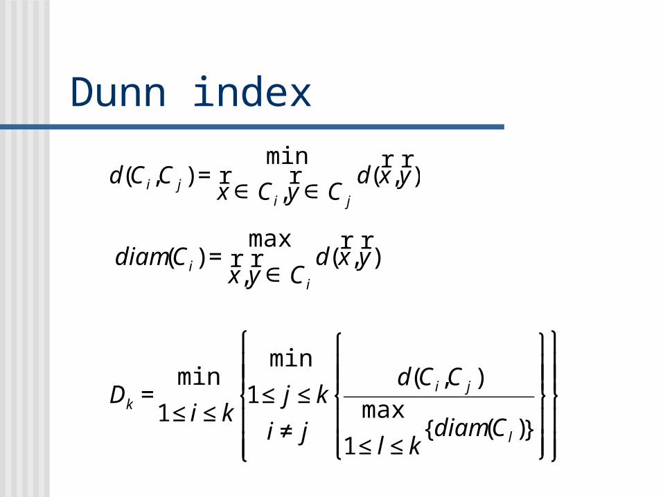
Dunn index
€
d(Ci,C j ) =min
r x ∈ Ci,
r y ∈ C j
d(r x ,
r y )
€
diam(Ci) =max
r x ,
r y ∈ Ci
d(r x ,
r y )
€
Dk =min
1≤ i ≤ k
min
1≤ j ≤ k
i ≠ j
d(Ci,C j )max
1≤ l ≤ kdiam(Cl ){ }
⎧
⎨ ⎪ ⎪
⎩ ⎪ ⎪
⎫
⎬ ⎪ ⎪
⎭ ⎪ ⎪
⎧
⎨ ⎪ ⎪
⎩ ⎪ ⎪
⎫
⎬ ⎪ ⎪
⎭ ⎪ ⎪
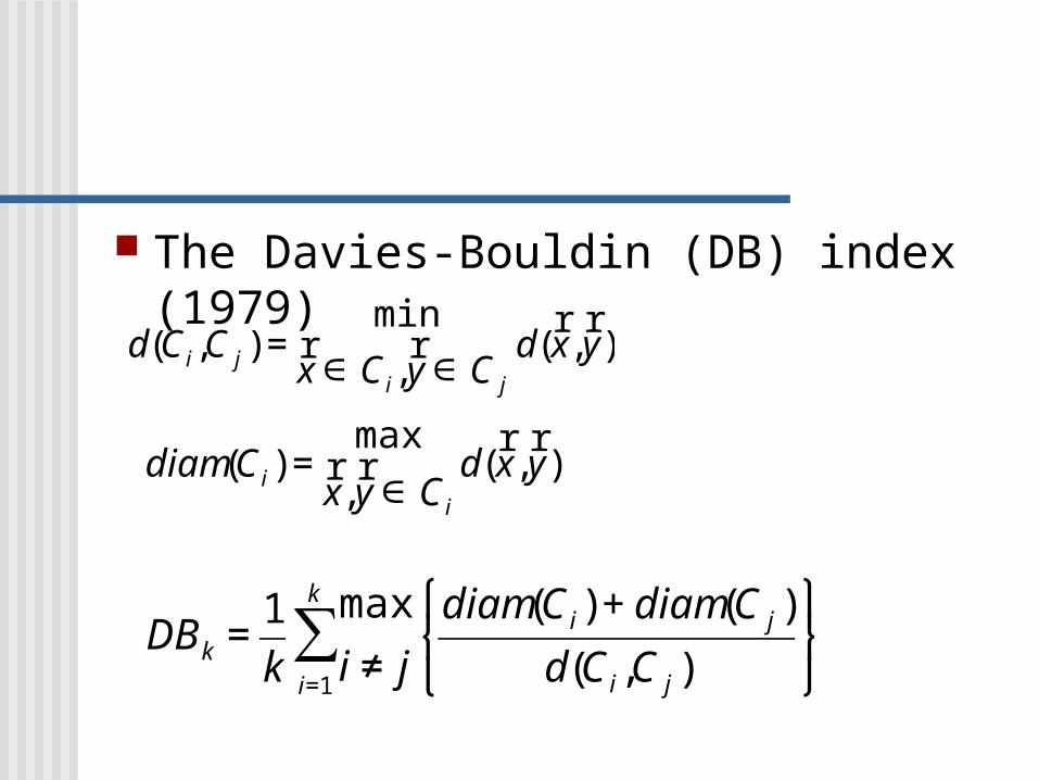
The Davies-Bouldin (DB) index (1979)
€
d(Ci,C j ) =min
r x ∈ Ci,
r y ∈ C j
d(r x ,
r y )
€
diam(Ci) =max
r x ,
r y ∈ Ci
d(r x ,
r y )
€
DBk =1
k
max
i ≠ j
diam(Ci) + diam(C j )
d(Ci,C j )
⎧ ⎨ ⎩
⎫ ⎬ ⎭i=1
k
∑

Pattern Classification (2nd ed.), Richard O. Duda,, Peter E. Hart, and David G. Stork, Wiley Interscience, 2001
Pattern Recognition: Concepts, Methods and Applications , Joaquim P. Marques de Sa, Springer-Verlag, 2001
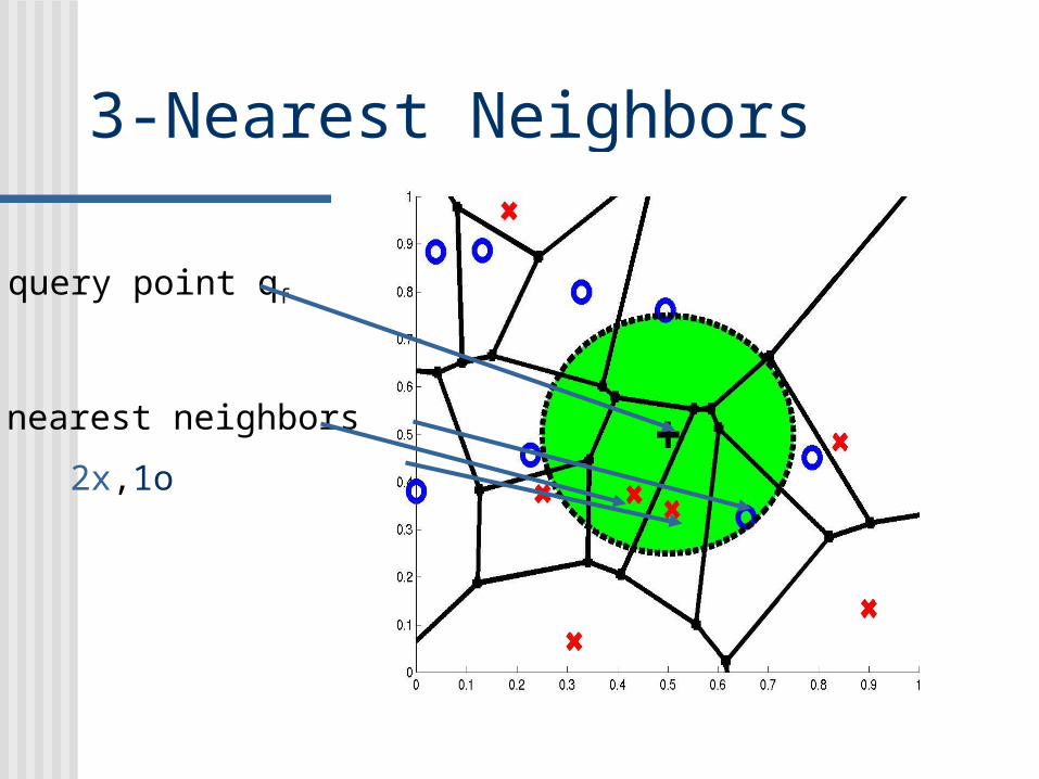
3-Nearest Neighbors
query point qf
3 nearest neighbors
2x,1o

Machine Learning, Tom M. Mitchell, McGraw Hill, 1997

Bayes
Naive Bayes
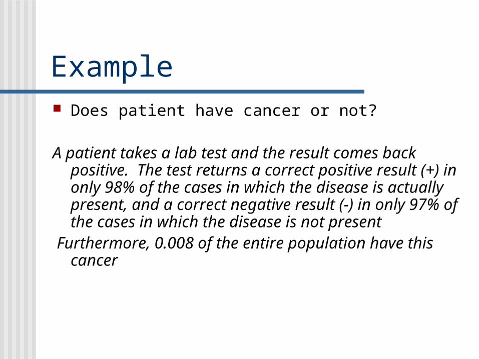
Example Does patient have cancer or not?
A patient takes a lab test and the result comes back positive. The test returns a correct positive result (+) in only 98% of the cases in which the disease is actually present, and a correct negative result (-) in only 97% of the cases in which the disease is not present
Furthermore, 0.008 of the entire population have this cancer
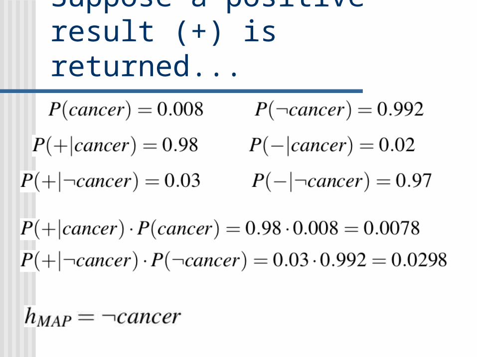
Suppose a positive result (+) is returned...
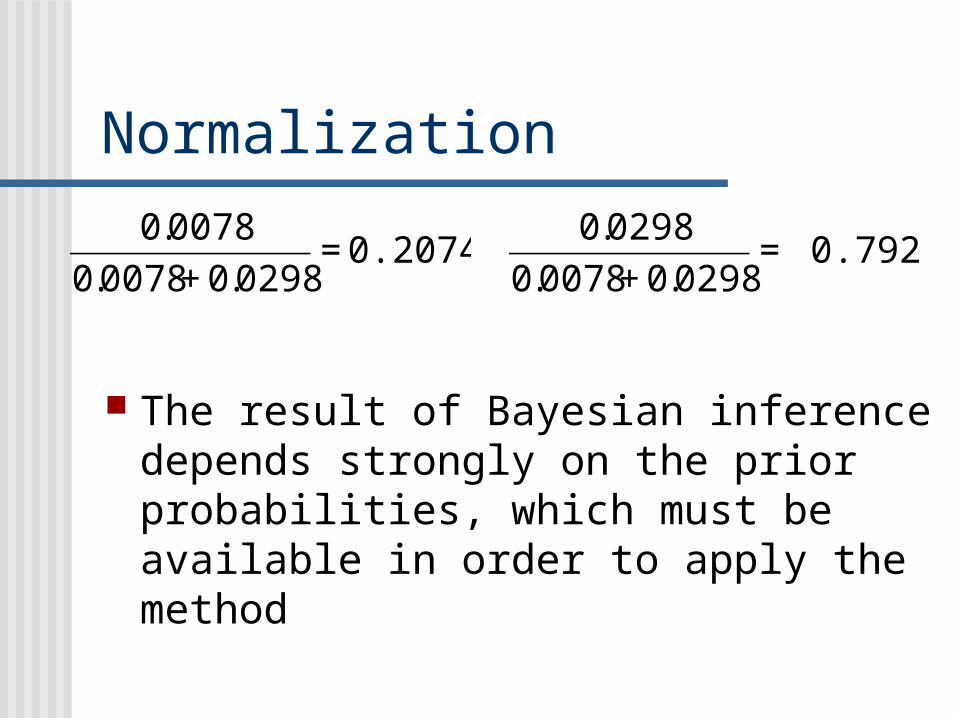
Normalization
The result of Bayesian inference depends strongly on the prior probabilities, which must be available in order to apply the method
€
0.0078
0.0078 + 0.0298= 0.20745
€
0.0298
0.0078 + 0.0298= 0.79255
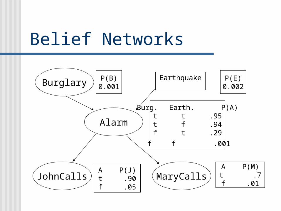
Belief Networks
Burglary P(B)0.001
Earthquake P(E)0.002
Alarm
Burg. Earth. P(A)t t .95t f .94f t .29
f f .001
JohnCalls MaryCallsA P(J)t .90f .05
A P(M)t .7f .01
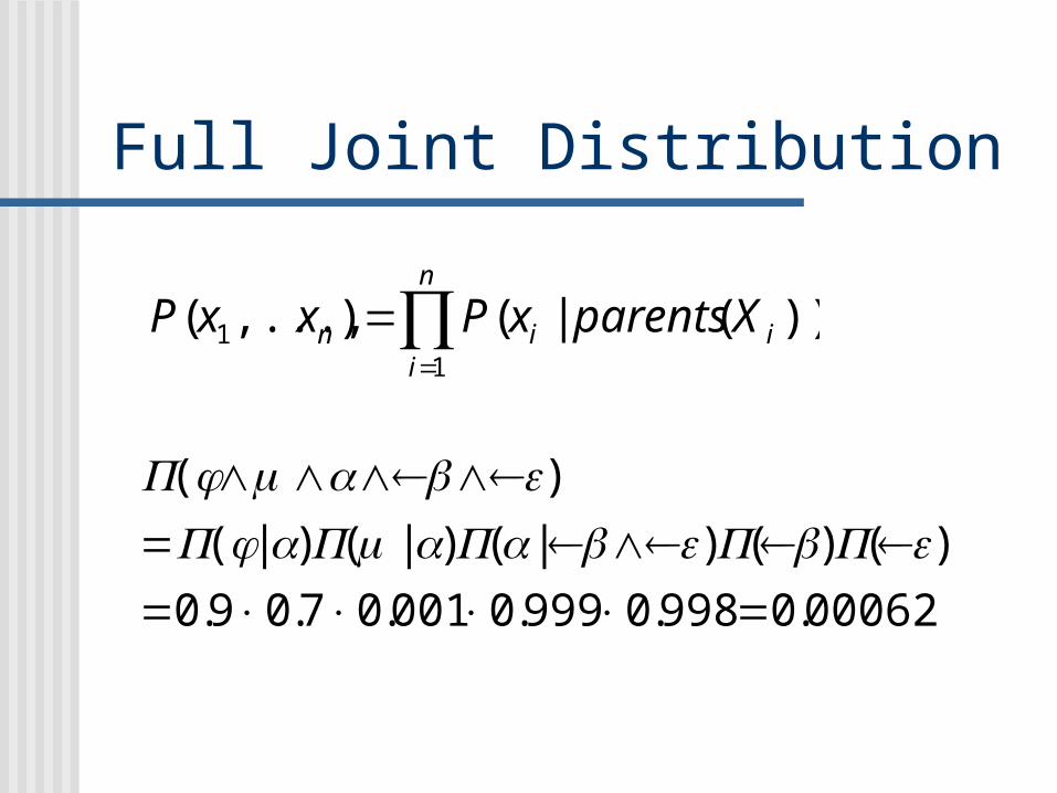
Full Joint Distribution
))(|(),...,(1
1 i
n
iin XparentsxPxxP ∏
=
=
00062.0998.0999.0001.07.09.0
)()()|()|()|(
)(
=××××=¬¬¬∧¬=
¬∧¬∧∧∧ePbPebaPamPajP
ebamjP
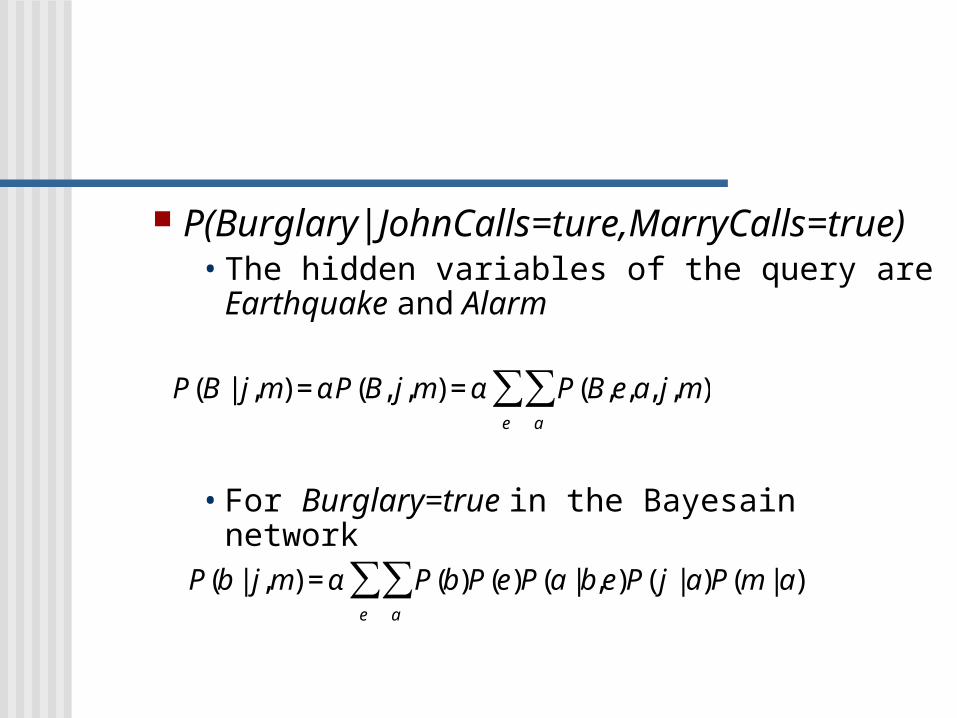
P(Burglary|JohnCalls=ture,MarryCalls=true)• The hidden variables of the query are Earthquake
and Alarm
• For Burglary=true in the Bayesain network
€
P(B | j,m) = αP(B, j,m) = α P(B,e,a, j,m)a
∑e
∑
€
P(b | j,m) = α P(b)P(e)P(a | b,e)P( j | a)P(m | a)a
∑e
∑
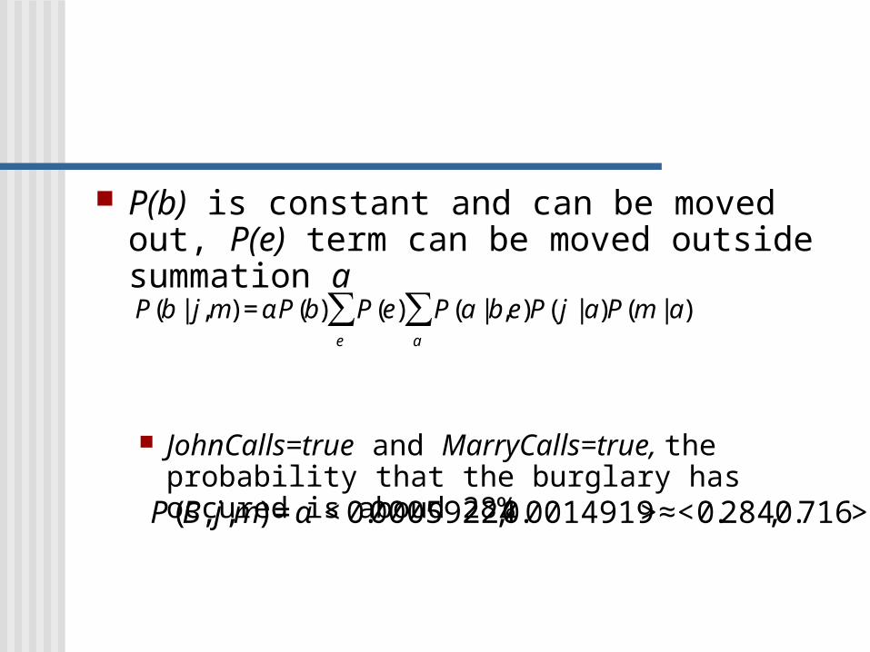
P(b) is constant and can be moved out, P(e) term can be moved outside summation a
JohnCalls=true and MarryCalls=true, the probability that the burglary has occured is aboud 28%€
P(b | j,m) = αP(b) P(e) P(a | b,e)P( j | a)P(m | a)a
∑e
∑
€
P(B, j,m) = α < 0.00059224,0.0014919 >≈< 0.284,0.716 >

Computation for Burglary=true
Zur Anzeige wird der QuickTime™ Dekompressor „TIFF (LZW)“
benötigt.

Artificial Intelligence - A Modern Approach, Second Edition, S. Russel and P. Norvig, Prentice Hall, 2003

ID3 - Tree learning

Zur Anzeige wird der QuickTime™ Dekompressor „TIFF (LZW)“
benötigt.
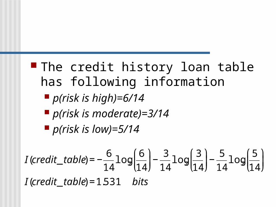
The credit history loan table has following information p(risk is high)=6/14 p(risk is moderate)=3/14 p(risk is low)=5/14
€
I(credit _ table) = −6
14log2
6
14
⎛
⎝ ⎜
⎞
⎠ ⎟−
3
14log2
3
14
⎛
⎝ ⎜
⎞
⎠ ⎟−
5
14log2
5
14
⎛
⎝ ⎜
⎞
⎠ ⎟
I(credit _ table) =1.531 bits
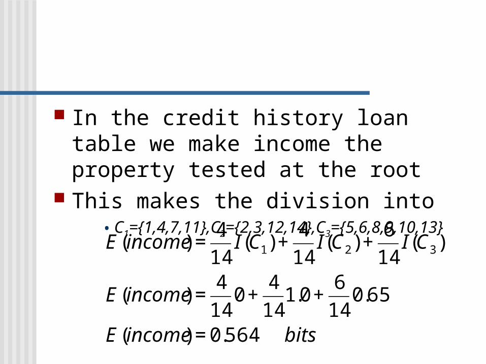
In the credit history loan table we make income the property tested at the root
This makes the division into• C1={1,4,7,11},C2={2,3,12,14},C3={5,6,8,9,10,13}
€
E(income) =4
14I(C1) +
4
14I(C2) +
6
14I(C3)
E(income) =4
140 +
4
141.0 +
6
140.65
E(income) = 0.564 bits
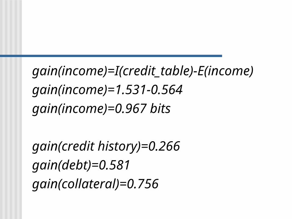
gain(income)=I(credit_table)-E(income)
gain(income)=1.531-0.564
gain(income)=0.967 bits
gain(credit history)=0.266
gain(debt)=0.581
gain(collateral)=0.756

Zur Anzeige wird der QuickTime™ Dekompressor „TIFF (LZW)“
benötigt.
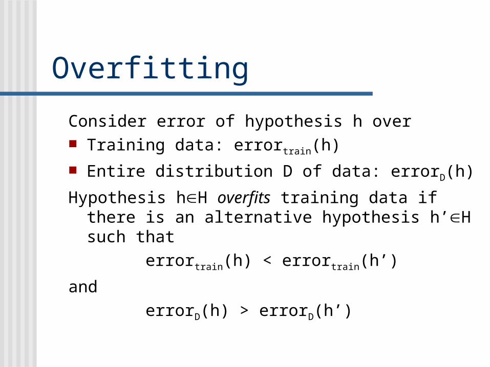
Overfitting
Consider error of hypothesis h over Training data: errortrain(h)
Entire distribution D of data: errorD(h)
Hypothesis hH overfits training data if there is an alternative hypothesis h’H such that
errortrain(h) < errortrain(h’)
and
errorD(h) > errorD(h’)
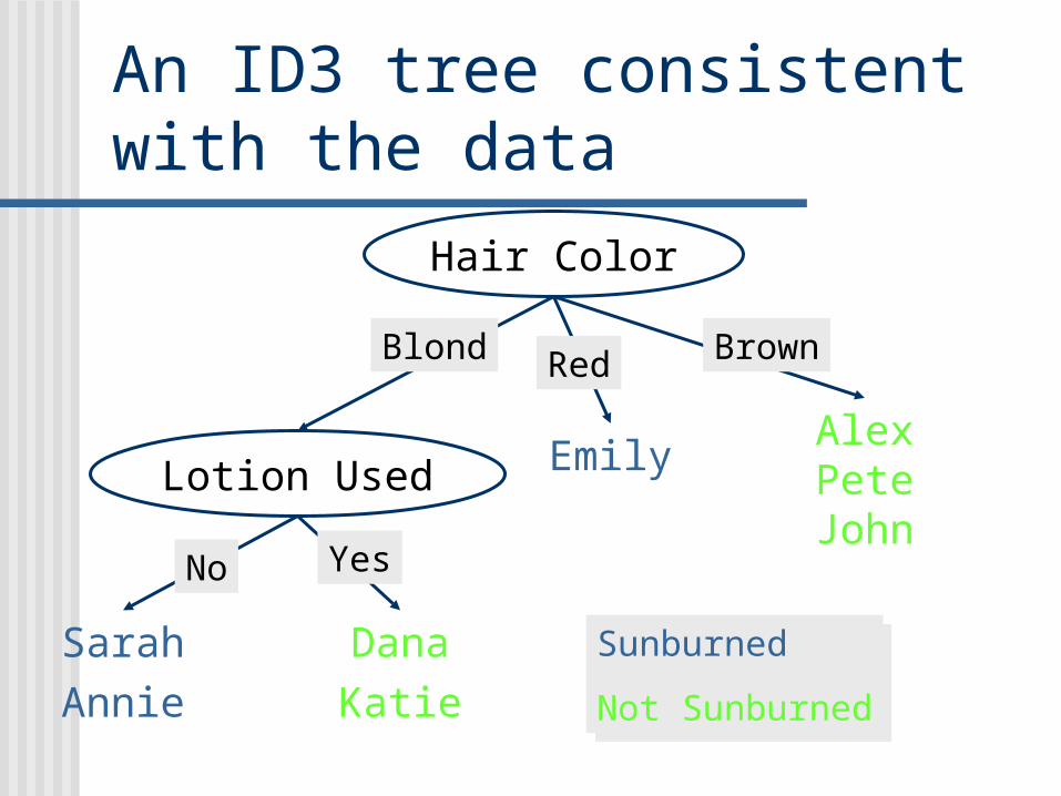
An ID3 tree consistent with the data
Hair Color
Lotion Used
Sarah
Annie
Dana
Katie
EmilyAlexPeteJohn
Blond Red Brown
No Yes
Sunburned
Not Sunburned
Sunburned
Not Sunburned
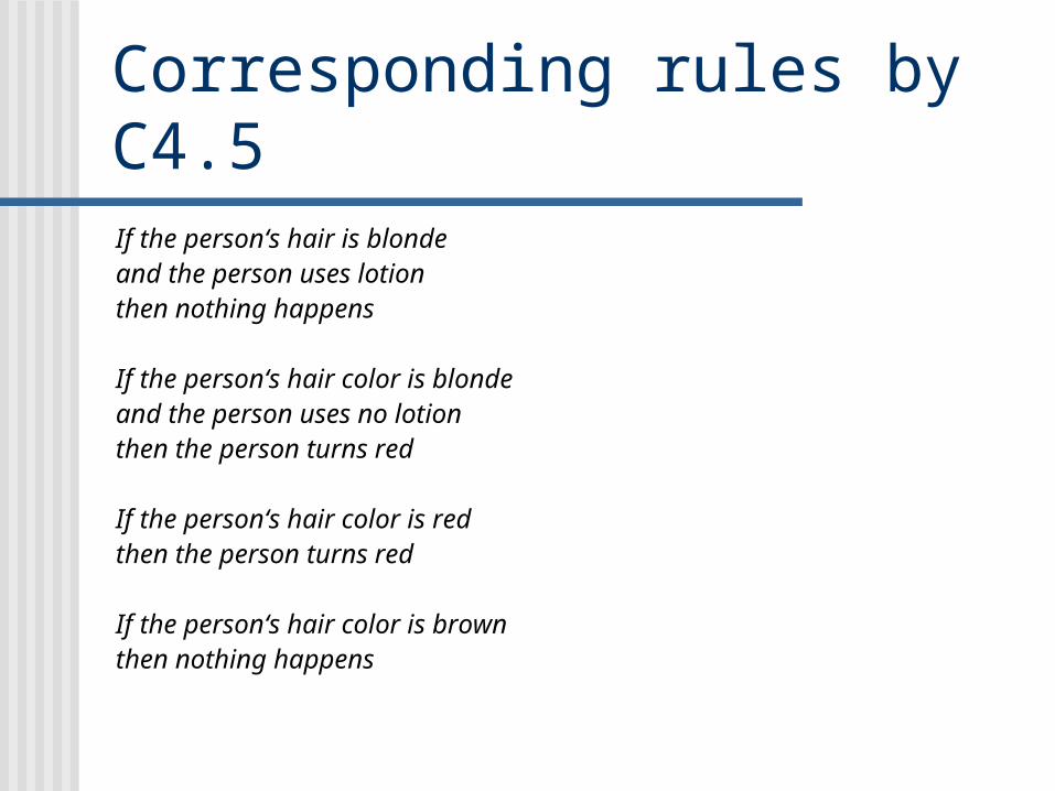
Corresponding rules by C4.5If the person‘s hair is blonde and the person uses lotionthen nothing happens
If the person‘s hair color is blonde and the person uses no lotionthen the person turns red
If the person‘s hair color is redthen the person turns red
If the person‘s hair color is brownthen nothing happens
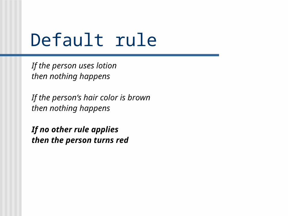
Default ruleIf the person uses lotionthen nothing happens
If the person‘s hair color is brownthen nothing happens
If no other rule appliesthen the person turns red
Artificial Intelligence, Partick Henry Winston, Addison-Wesley, 1992
Artificial Intelligence - Structures and Strategies for Complex Problem Solving, Second Edition, G. L. Luger and W. A. Stubblefield, Benjamin/Cummings Publishing, 1993
Machine Learning, Tom M. Mitchell, McGraw Hill, 1997
Perceptron
Limitations Gradient descent
XOR problem and Perceptron
By Minsky and Papert in mid 1960
Zur Anzeige wird der QuickTime™ Dekompressor „TIFF (LZW)“
benötigt.
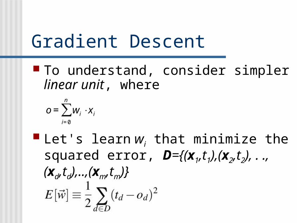
Gradient Descent To understand, consider simpler linear
unit, where
Let's learn wi that minimize the squared error, D={(x1,t1),(x2,t2), . .,(xd,td),..,(xm,tm)}
• (t for target)€
o = wi ⋅ x i
i= 0
n
∑
Feed-forward networks
Back-Propagation Activation Functions

Zur Anzeige wird der QuickTime™ Dekompressor „TIFF (LZW)“
benötigt.
xk
x1 x2 x3 x4 x5
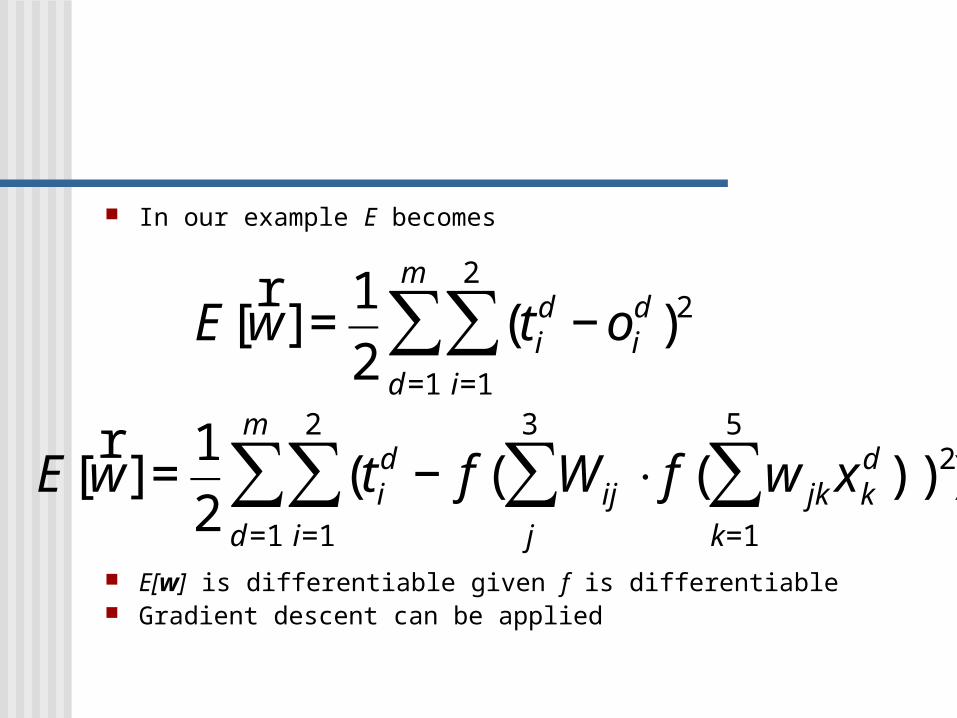
In our example E becomes
E[w] is differentiable given f is differentiable Gradient descent can be applied
€
E[r w ] =
1
2(ti
d
i=1
2
∑d =1
m
∑ − oid )2
€
E[r w ] =
1
2(ti
d
i=1
2
∑d =1
m
∑ − f ( W ij
j
3
∑ ⋅ f ( w jk xkd
k=1
5
∑ )))2
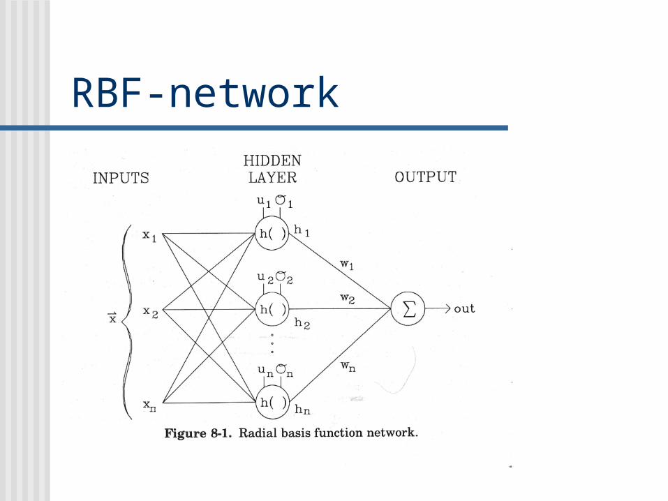
RBF-network
RBF-networks Support Vector Machines
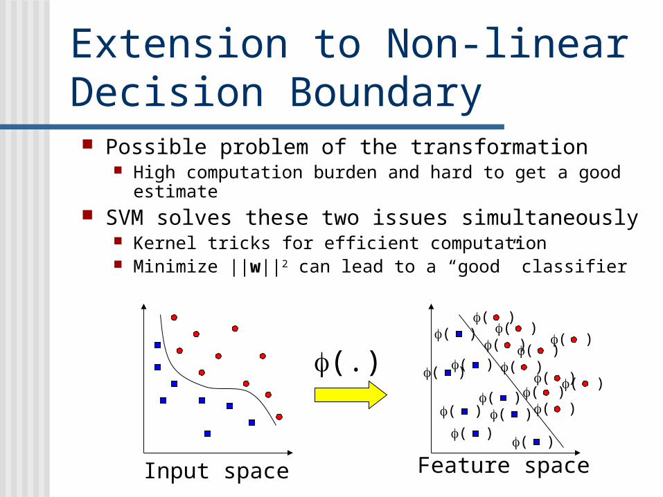
Extension to Non-linear Decision Boundary Possible problem of the transformation
High computation burden and hard to get a good estimate SVM solves these two issues simultaneously
Kernel tricks for efficient computation Minimize ||w||2 can lead to a “good” classifier
( )
( )
( )( )( )
( )
( )( )
(.)( )
( )
( )
( )( )
( )
( )
( )( )
( )
Feature spaceInput space
Machine Learning, Tom M. Mitchell, McGraw Hill, 1997
Simon Haykin, Neural Networks, Secend edition Prentice Hall, 1999