Overhaul Overdraft Fees: Creating Pricing and ProductDesign Strategies with Big Data∗

Xiao Liu, Alan Montgomery, Kannan Srinivasan

October 12, 2014

AbstractIn 2012, consumers paid an enormous $32 billion overdraft fees. Consumer attrition and

potential government regulations to shut down the overdraft service urge banks to come upwith financial innovations to overhaul the overdraft fees. However, no empirical research hasbeen done to explain consumers’ overdraft incentives and evaluate alternative pricing and prod-uct strategies. In this paper, we build a dynamic structural model with consumer monitoringcost and dissatisfaction. We find that on one hand, consumers heavily discount the future andoverdraw because of impulsive spending. On the other hand, a high monitoring cost makes ithard for consumers to track their finances therefore they overdraw because of rational inatten-tion. In addition, consumers are dissatisfied by the overly high overdraft fee and close theiraccounts. We apply the model to a big dataset of more than 500,000 accounts for a span of 450days. Our policy simulations show that alternative pricing strategies may increase the bank’srevenue. Sending targeted and dynamic alerts to consumers can not only help consumers avoidoverdraft fees but improve bank profits from higher interchange fees and less consumer attri-tion. To alleviate the computational burden of solving dynamic programming problems on alarge scale, we combine parallel computing techniques with a Bayesian Markov Chain MonteCarlo algorithm. The Big Data allow us to detect the rare event of overdraft and reduce thesampling error with minimal computational costs.

1 IntroductionAn overdraft occurs when a consumer attempts to spend or withdraw funds from her checkingaccounts in an amount exceeding the account’s available funds. In the US, banks allow consumersto overdraw their accounts (subject to some restrictions at banks’ discretion) and charge an over-draft fee. Overdraft fees have become a major source of bank revenues since banks started tooffer free checking accounts to attract consumers. In 2012, the total amount of overdraft fees inthe US reached $32 billion, according to Moebs Services1. This is equivalent to an average of$178 for each checking account annually2. According to the Center for Responsible Lending, UShouseholds spent more on overdraft fees than on fresh vegetables, postage and books in 2010.3

∗We acknowledge support from the Dipankar and Sharmila Chakravarti Fellowship. All errors are our own.1http://www.moebs.com2According to Evans, Litan, and Schmalensee 2011, there are 180 million checking accounts in the US.3http://www.blackenterprise.com/money/managing-credit-3-ways-overdraft-fees-will-still-haunt-you/

1

The unfairly high overdraft fee has provoked a storm of consumer outrage and therefore causedmany consumers to close the account. The US government has taken actions to regulate theseoverdraft fees through the Consumer Financial Protection Agency4 and may potentially shut downthe overdraft service5. Without overhauling the current overdraft fee, banks encounter the problemof losing valuable customers and possibly totally losing the revenue source from overdrafts.

Financial institutions store massive amounts of information about consumers. The advantagesof technology and Big Data enable banks to reverse the information asymmetry (Kamenica, Mul-lainathan, and Thaler 2011) as they may be able to generate better forecasts about a consumer’sfinancial state than consumers themselves can. In this paper, we extract the valuable informationembedded in the Big Data and harness it with structural economic theories to explain consumers’overdraft behavior. The large scale financial transaction panel data allows us to sort through con-sumers’ financial decision making processes and discover rich consumer heterogeneity. As a con-sequence, we come up with individually customized strategies that can increase both consumerwelfare and bank revenue.

In this paper, we aim to achieve two substantive goals. First, we leverage rich data about con-sumer spending and balance checking to understand the decision process for consumers to over-draw. We address the following research questions. Are consumers fully attentive in monitoringtheir checking account balances? How great is the monitoring cost? Why do attentive consumersalso overdraw? Are consumers dissatisfied because the overdraft fee?

Second, we investigate pricing and new product design strategies that overhaul overdraft fees.Specifically, we tackle these questions. Is the current overdraft fee structure optimal? How willthe bank revenue change under alternative pricing strategies? More importantly, what new revenuemodel can make the incentives of the bank and consumers better aligned? Can the bank benefitfrom helping consumers make more informed financial decisions, like sending alerts to consumers?If so, what’s the optimal alert strategy? How can the bank leverage its rich data about consumerfinancial behaviors to reverse information asymmetry and create targeted strategies?

We estimate the dynamic structural model using data from a large commercial bank in theUS. The sample size is over 500,000 accounts and the sample length is up to 450 days. We findthat some consumers are inattentive in monitoring their finances because of a substantially highmonitoring cost. In contrast, attentive consumers overdraw because they heavily discount futureutilities and are subject to impulsive spending. Consumers are dissatisfied to leave the bank afterbeing charged the unfairly high overdraft fees. In our counterfactual analysis, we show that apercentage fee or a quantity premium fee strategy can achieve higher bank revenue compared tothe current flat per-transaction fee strategy. Enabled by Big Data, we also propose an optimaltargeted alert strategy. The bank can benefit from sending alerts to let consumers spend theirunused balances so that the bank can earn more interchange fees. Helping consumers make moreinformed decisions will also significantly reduce consumer attrition. The targeted dynamic alertsshould be sent to consumers with higher monitoring costs and both when they are underspendingand overspending.

Methodologically, our paper makes two key contributions. First, we build a dynamic struc-tural model that incorporates inattention and dissatisfaction into the life-time consumption model.Although we apply it to the overdraft context, the model framework can be generalized to ana-

4http://banking-law.lawyers.com/consumer-banking/consumers-and-congress-tackle-big-bank-fees.html5http://files.consumerfinance.gov/f/201306_cfpb_whitepaper_overdraft-practices.pdf

2

lyze other marketing problems regarding consumer dynamic budget allocation, like electricity andcellphone usage.

Second, we estimate the model on Big Data with the help of parallel computing techniques.Structural models have the merit of producing policy invariate parameters that allow us to conductcounterfactual analysis. However, the inherent computational burden prevents it from being widelyadopted by industries. Moreover, the data size in a real setting is typically much larger than what’sused for research purposes. Companies, in our case a large bank, need to have methods that areeasily scalable to generate targeted solutions for each consumer. Our proposed algorithm takesadvantage of state-of-the-art parallel computing techniques and estimation methods that alleviatecomputational burden and reduce the curse of dimensionality.

The rest of the paper is organized as follows. In section 2 we first review related literature.Then we show summary statistics in section 3 which motivate our model setup. Section 4 describesour structural model and we provide details of identification and estimation procedures in section5. Then in sections 6 and 7 we show estimation results and counterfactual analysis. Section 8concludes and summarizes our limitations.

2 Related LiteratureA variety of economic and psychological models can explain overdrafts, including full-informationpure rational models and limited attention, as summarized by Stango and Zinman (2014). However,no empirical paper has applied these theories to real consumer spending data. Although Stangoand Zinman (2014) had a similar dataset to ours, their focus was on testing whether taking relatedsurveys can reduce overdrafts. We develop a dynamic structural model that incorporates theoriesof heavy discounting, inattention and dissatisfaction in a comprehensive framework. The model isflexible to address various overdraft scenarios, thus it can be used by policy makers and the bankto design targeted strategies to increase consumer welfare and bank revenue.

Our model inherits from the traditional lifetime consumption model but adds two novel fea-tures, inattention and dissatisfaction. First of all, a large body of literature in psychology andeconomics has found that consumers pay limited attention to relevant information. In the reviewpaper by Card, DellaVigna and Malmendier (2011), they summarize findings indicating that con-sumers pay limited attention to 1) shipping costs, 2) tax (Chetty et. al. 2009) and 3) ranking (Pope2009). Gabaix and Laibson (2006) find that consumers don’t pay enough attention to add-on pric-ing and Grubb (2014) shows consumers’ inattention to their cell-phone minute balances. Manypapers in the finance and accounting domain have documented that investors and financial analystsare inattentive to various financial information (e.g., Hirshleifer and Teoh 2003, Peng and Xiong2006). We follow Stango and Zinman (2014) to define inattention as incomplete consideration ofaccount balances (realized balance and available balance net of coming bills) that would informchoices. We further explain inattention with a structural parameter, monitoring cost, which repre-sents the time and effort to know the exact amount of money in the checking account. With thisparameter estimated, we are able to quantify the economic value of sending alerts to consumersand provide guidance for the bank to set its pricing strategy. We also come up with policy simu-lations about alerts because we think a direct remedy for consumers’ limited attention is to makeinformation more salient (Card, DellaVigna and Malmendier 2011). Past literature also finds thatreminders (Karlan et. al. 2010), mandatory disclosure (Fishman and Hagerty 2003), and penal-

3

ties (Haselhuhn et al. 2012) all serve the purpose of increasing salience and thus mitigating thenegative consequences of inattention.

Second, as documented in previous literature, unfairly high price may cause consumer dissat-isfaction which is one of the main causes of customer switching behavior (Keaveney 1995, Bolton1998). We notice that consumers are more likely to close the account after paying the overdraftfee and when the ratio of the overdraft fee over the overdraft transaction amount is high. This isbecause given the current banking industry practice, a consumer pays a flat per-transaction fee re-gardless of the transaction amount. Therefore, the implied interest rate for an overdraft originatedby a small transaction amount is much higher than the socially accepted interest rate (Matzler,Wurtele and Renzl 2006), leading to price dissatisfaction.

We aim to estimate this infinite horizon dynamic structural model on a large scale of data andobtain heterogeneous best response for each consumer to prepare targeted marketing strategies.After searching among different estimation methods, including the nested fixed point algorithm(Rust 1987), the conditional choice probability estimation (Arcidiacono and Miller 2011) and theBayesian estimation method developed in Imai, Jain and Ching (2009) (IJC), we finally choose theIJC method for the following reasons. First of all, the hierarchical Bayes framework fits our goal ofobtaining heterogeneous parameters. Second, in order to apply our model to a large scale of data,we need to estimate the model with Bayesian MCMC so that we can implement a parallel comput-ing technique. Third, IJC is the state-of-the art Bayesian estimation algorithm for infinite horizondynamic programming models. It provides two additional benefits in tackling the computationalchallenges. One is that it alleviates the computational burden by only evaluating the value func-tion once in each MC iteration. Essentially, the algorithm solves the value function and estimatesthe structural parameters simultaneously. So the computational burden of a dynamic problem isreduced by an order of magnitude similar to those computational costs of a static model. The otheris that the method reduces the curse of dimensionality by allowing state space grid points to varybetween estimation iterations. On the other hand, as our sample size is huge, traditional MCMCestimation may take a prohibitively, if not impossibly, long time, since for N data points, mostmethods must perform O(N) operations to draw a sample. A natural way to reduce the compu-tation time is to run the chain in parallel. Past methods of Parallel MCMC duplicate the data onmultiple machines and cannot reduce the time of burn-in. We instead use a new technique devel-oped by Neiswanger, Wang and Xing (2014) to solve this problem. The key idea of this algorithmis that we can distribute data into multiple machines and perform IJC estimation in parallel. Oncewe obtain the posterior Markov Chains from each machine, we can algorithmically combine theseindividual chains to get the posterior chain of the whole sample.

3 Background and Model Free EvidenceWe obtained data from a major commercial bank in the US. During our sample period in 2012 and2013, overdraft fees accounted for 47% of the revenue from deposit account service charges and9.8% of the operating revenue.

The bank provides a comprehensive overdraft solution to consumers. (For general overdraftpractices in the US, please refer to Stango and Zinman (2014) for a good review. Appendix A.1tabulates current fee settings in top US banks.) In the standard overdraft service, if the consumer

4

overdraws her account, the bank might cover the transaction and charge $316 Overdraft Fee (OD)or decline the transaction and charge a $31 Non-Sufficient-Fund Fee (NSF). Whether the transac-tion is accepted or declined is at the bank’s discretion. The OD/NSF fee is at a per-item level. Ifa consumer performs several transactions when the account is already overdrawn, each transactionitem will incur a fee of 31 dollars. Within a day, a maximum of four per-item fees can be charged.If the account remains overdrawn for five or more consecutive calendar days, a Continuous Over-draft Fee of $6 will be assessed up to a maximum of $84. The bank also provides an OverdraftProtection Service where the checking account can link to another checking account, a credit cardor a line of credit. In this case, when the focal account is overdrawn, funds can be transferred tocover the negative balance. The Overdraft Transfer Balance Fee is $9 for each transfer. As you cansee, the fee structure for the bank is quite complicated. In the empirical analysis below, we don’tdistinguish between different types of overdraft fees and assume that money is fungible so thatthe consumer only cares about the total amount of overdraft fee rather than the underlying pricingstructure.

The bank also provides balance checking services through branch, automated teller machine(ATM), call center and online/mobile banking. Consumers can inquire about their available bal-ances and recent activities. There’s also a notification service to consumers via email or textmessage, named “alerts”. Consumers can set alerts when certain events take place, like overdrafts,insufficient funds, transfers, deposits, etc. Unfortunately, our dataset only includes the balancechecking data but not the alert data. We’ll discuss this limitation in section 8.

In 2009, the Federal Reserve Board made an amendment to Regulation E (subsequently re-codified by the Consumer Financial Protection Bureau (CFPB)) which requires account holdersto provide affirmative consent (opt in) for overdraft coverage of ATM and non-recurring point ofsale (POS) debit card transactions before banks can charge for paying such transactions7. ThisRegulation E aimed to protect consumers against the heavy overdraft fees. The change becameeffective for new accounts on July 1, 2010, and for existing accounts on August 15, 2010. Oursample contains both opt-in and opt-out accounts. However, we don’t know which accounts haveopted in unless we observe an ATM/POS initiated overdraft occasion. We also discuss this datalimitation in section 8.

3.1 Summary StatisticsOur data can be divided into two categories, checking account transactions and balance inquiry ac-tivities. In our sample, there are between 500,000 and 1,000,0008 accounts, among which 15.8%had at least one overdraft incidence during the sample period between June 2012 and Aug 2013.The proportion of accounts with overdraft is lower than the 27% (across all banks and credit unions)reported by the CFPB in 20129. In total, all the counts performed more than 200 million transac-tions, including deposits, withdrawals, transfers, and payments etc. For each transaction, we knowthe account number, transaction date, transaction amount, and transaction description. The transac-

6All dollar values in the paper have been rescaled by a number between .85 and 1.15 to help obfuscate the ex-act amounts without changing the substantive implications. The bank also sets the first time overdraft fee for eachconsumer at $22. All the rest overdraft fees are set at $31.

7http://www.occ.gov/news-issuances/bulletins/2011/bulletin-2011-43.html8For the sake of privacy, we can’t disclose the exact number.9http://files.consumerfinance.gov/f/201306_cfpb_whitepaper_overdraft-practices.pdf

5

tion description tells us the type of transaction (e.g., ATM withdrawal or debit card purchase) andlocation/associated institution of the transaction, like merchant name or branch location. The de-scription helps us identify the cause of the overdraft, for instance whether it’s due to an electricitybill or due to a grocery purchase.

Table 1: Overdraft Frequency and Fee DistributionMean Std Median Min 99.85 Percentile

OD Frequency 9.84 18.74 3 1 >100OD Fee 245.46 523.04 77 10 >2730

As shown in Table 1, consumers who paid overdraft fees, on average, overdrew nearly 10 timesand paid $245 during the 15 month sample period. This is consistent with the finding from theCFPB that the average overdraft- and NSF-related fees paid by all accounts that had one or moreoverdraft transactions in 2011 were $22510. There is significant heterogeneity in consumers’ over-draft frequency and the distribution of overdraft frequency is quite skewed. The median overdraftfrequency is three and more than 25% of consumers overdrew only once. In contrast, the top0.15% of heavy overdrafters overdrew more than 100 times. A similar skewed pattern applies tothe distribution of overdraft fees. While the median overdraft fee is $77, the top 0.15% of heaviestoverdrafters paid more than $2,730 in fees.

Figure 1: Overdraft Frequency and Fee Distribution

Now let’s zoom in to take a look at the behavior of the majority overdrafters that have over-drawn less than 40 times. The first panel in Figure 1 depicts the distribution of overdraft frequencyfor those accounts. Notice that most consumers (> 50%) only overdrew less than three times. Thesecond panel shows the distribution of the paid overdraft fee for accounts that have overdrawn lessthan $300. Consistent with the fee structure where the standard per-item overdraft fee is $22 or$31, we see spikes on these two numbers and their multiples.

10http://files.consumerfinance.gov/f/201306_cfpb_whitepaper_overdraft-practices.pdf

6

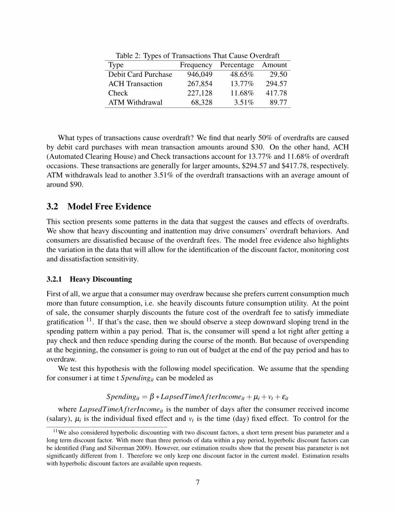
Table 2: Types of Transactions That Cause OverdraftType Frequency Percentage AmountDebit Card Purchase 946,049 48.65% 29.50ACH Transaction 267,854 13.77% 294.57Check 227,128 11.68% 417.78ATM Withdrawal 68,328 3.51% 89.77

What types of transactions cause overdraft? We find that nearly 50% of overdrafts are causedby debit card purchases with mean transaction amounts around $30. On the other hand, ACH(Automated Clearing House) and Check transactions account for 13.77% and 11.68% of overdraftoccasions. These transactions are generally for larger amounts, $294.57 and $417.78, respectively.ATM withdrawals lead to another 3.51% of the overdraft transactions with an average amount ofaround $90.

3.2 Model Free EvidenceThis section presents some patterns in the data that suggest the causes and effects of overdrafts.We show that heavy discounting and inattention may drive consumers’ overdraft behaviors. Andconsumers are dissatisfied because of the overdraft fees. The model free evidence also highlightsthe variation in the data that will allow for the identification of the discount factor, monitoring costand dissatisfaction sensitivity.

3.2.1 Heavy Discounting

First of all, we argue that a consumer may overdraw because she prefers current consumption muchmore than future consumption, i.e. she heavily discounts future consumption utility. At the pointof sale, the consumer sharply discounts the future cost of the overdraft fee to satisfy immediategratification 11. If that’s the case, then we should observe a steep downward sloping trend in thespending pattern within a pay period. That is, the consumer will spend a lot right after getting apay check and then reduce spending during the course of the month. But because of overspendingat the beginning, the consumer is going to run out of budget at the end of the pay period and has tooverdraw.

We test this hypothesis with the following model specification. We assume that the spendingfor consumer i at time t Spendingit can be modeled as

Spendingit = β ∗LapsedTimeA f terIncomeit +µi + vt + εit

where LapsedTimeA f terIncomeit is the number of days after the consumer received income(salary), µi is the individual fixed effect and vt is the time (day) fixed effect. To control for the

11We also considered hyperbolic discounting with two discount factors, a short term present bias parameter and along term discount factor. With more than three periods of data within a pay period, hyperbolic discount factors canbe identified (Fang and Silverman 2009). However, our estimation results show that the present bias parameter is notsignificantly different from 1. Therefore we only keep one discount factor in the current model. Estimation resultswith hyperbolic discount factors are available upon requests.

7

effect that consumers usually pay for their bills (utilities, phone bills, credit card bills, etc) aftergetting the pay check, we exclude checks and ACH transactions which are the common choicesfor bill payments from the daily spendings and only keep debit card purchases, ATM withdrawalsand person-to-person transfers.

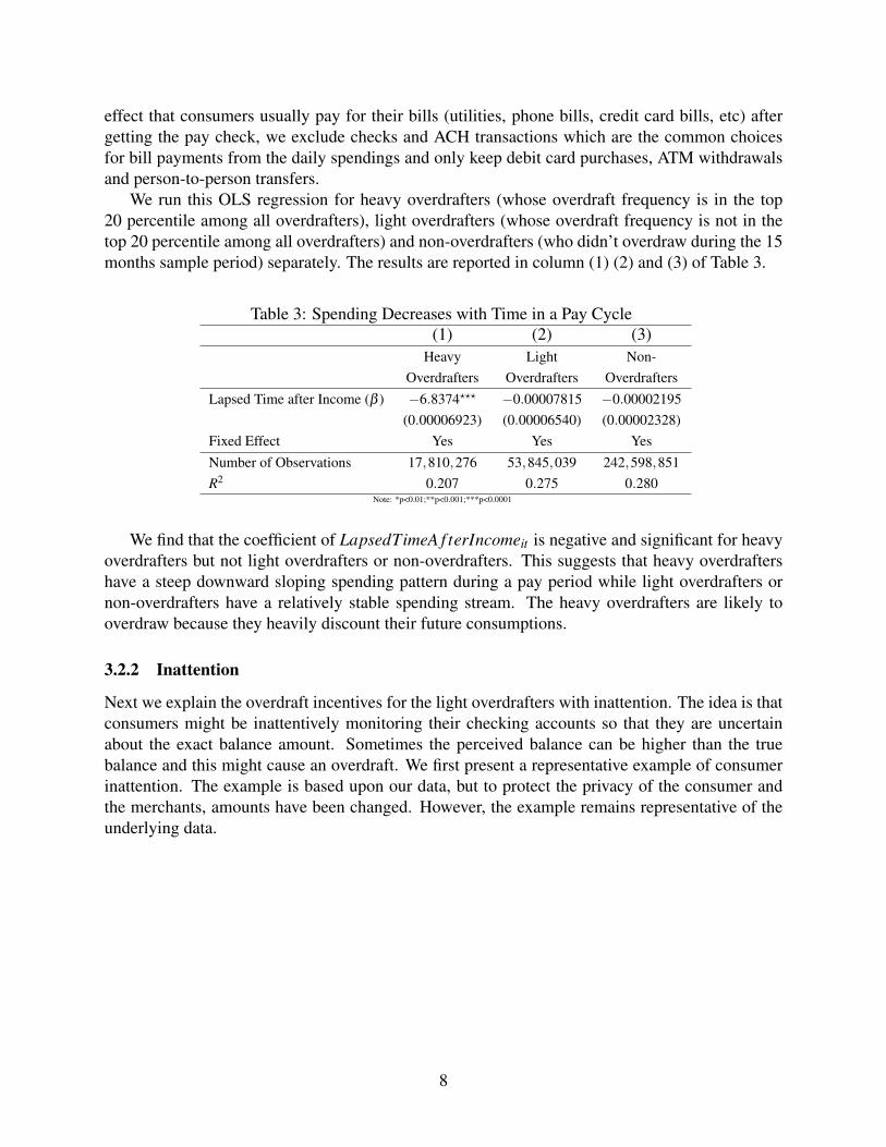
We run this OLS regression for heavy overdrafters (whose overdraft frequency is in the top20 percentile among all overdrafters), light overdrafters (whose overdraft frequency is not in thetop 20 percentile among all overdrafters) and non-overdrafters (who didn’t overdraw during the 15months sample period) separately. The results are reported in column (1) (2) and (3) of Table 3.

Table 3: Spending Decreases with Time in a Pay Cycle(1) (2) (3)

HeavyOverdrafters

LightOverdrafters

Non-Overdrafters

Lapsed Time after Income (β ) −6.8374??? −0.00007815 −0.00002195(0.00006923) (0.00006540) (0.00002328)

Fixed Effect Yes Yes YesNumber of Observations 17,810,276 53,845,039 242,598,851R2 0.207 0.275 0.280

Note: *p<0.01;**p<0.001;***p<0.0001

We find that the coefficient of LapsedTimeA f terIncomeit is negative and significant for heavyoverdrafters but not light overdrafters or non-overdrafters. This suggests that heavy overdraftershave a steep downward sloping spending pattern during a pay period while light overdrafters ornon-overdrafters have a relatively stable spending stream. The heavy overdrafters are likely tooverdraw because they heavily discount their future consumptions.

3.2.2 Inattention

Next we explain the overdraft incentives for the light overdrafters with inattention. The idea is thatconsumers might be inattentively monitoring their checking accounts so that they are uncertainabout the exact balance amount. Sometimes the perceived balance can be higher than the truebalance and this might cause an overdraft. We first present a representative example of consumerinattention. The example is based upon our data, but to protect the privacy of the consumer andthe merchants, amounts have been changed. However, the example remains representative of theunderlying data.

8

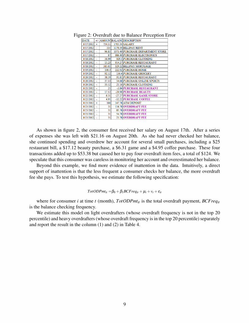
Figure 2: Overdraft due to Balance Perception Error

As shown in figure 2, the consumer first received her salary on August 17th. After a seriesof expenses she was left with $21.16 on August 20th. As she had never checked her balance,she continued spending and overdrew her account for several small purchases, including a $25restaurant bill, a $17.12 beauty purchase, a $6.31 game and a $4.95 coffee purchase. These fourtransactions added up to $53.38 but caused her to pay four overdraft item fees, a total of $124. Wespeculate that this consumer was careless in monitoring her account and overestimated her balance.

Beyond this example, we find more evidence of inattention in the data. Intuitively, a directsupport of inattention is that the less frequent a consumer checks her balance, the more overdraftfee she pays. To test this hypothesis, we estimate the following specification:

TotODPmtit =β0 +β1BCFreqit +µi + vt + εit

where for consumer i at time t (month), TotODPmtit is the total overdraft payment, BCFreqitis the balance checking frequency.

We estimate this model on light overdrafters (whose overdraft frequency is not in the top 20percentile) and heavy overdrafters (whose overdraft frequency is in the top 20 percentile) separatelyand report the result in the column (1) and (2) in Table 4.

9

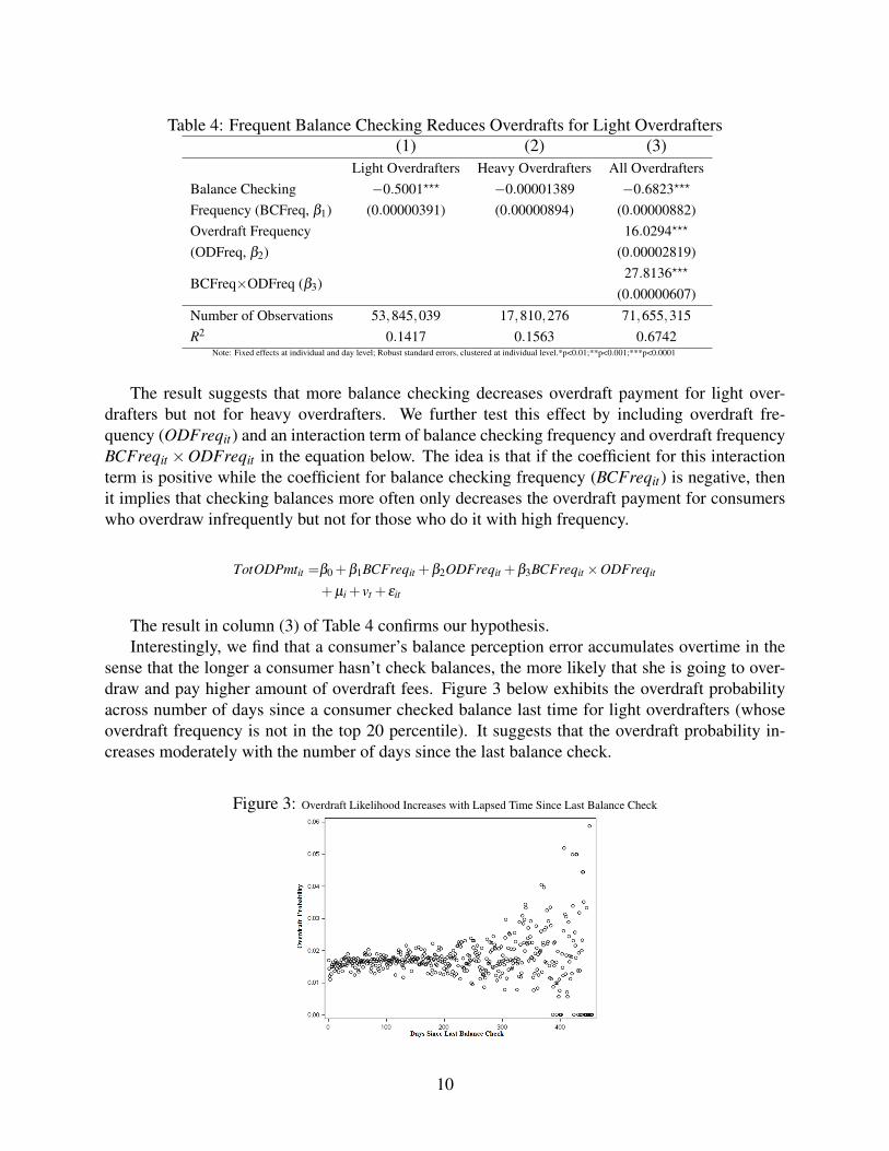
Table 4: Frequent Balance Checking Reduces Overdrafts for Light Overdrafters(1) (2) (3)

Light Overdrafters Heavy Overdrafters All OverdraftersBalance CheckingFrequency (BCFreq, β1)

−0.5001??? −0.00001389 −0.6823???

(0.00000391) (0.00000894) (0.00000882)Overdraft Frequency(ODFreq, β2)

16.0294???

(0.00002819)

BCFreq×ODFreq (β3)27.8136???

(0.00000607)Number of Observations 53,845,039 17,810,276 71,655,315R2 0.1417 0.1563 0.6742

Note: Fixed effects at individual and day level; Robust standard errors, clustered at individual level.*p<0.01;**p<0.001;***p<0.0001

The result suggests that more balance checking decreases overdraft payment for light over-drafters but not for heavy overdrafters. We further test this effect by including overdraft fre-quency (ODFreqit) and an interaction term of balance checking frequency and overdraft frequencyBCFreqit ×ODFreqit in the equation below. The idea is that if the coefficient for this interactionterm is positive while the coefficient for balance checking frequency (BCFreqit) is negative, thenit implies that checking balances more often only decreases the overdraft payment for consumerswho overdraw infrequently but not for those who do it with high frequency.

TotODPmtit =β0 +β1BCFreqit +β2ODFreqit +β3BCFreqit ×ODFreqit

+µi + vt + εit

The result in column (3) of Table 4 confirms our hypothesis.Interestingly, we find that a consumer’s balance perception error accumulates overtime in the

sense that the longer a consumer hasn’t check balances, the more likely that she is going to over-draw and pay higher amount of overdraft fees. Figure 3 below exhibits the overdraft probabilityacross number of days since a consumer checked balance last time for light overdrafters (whoseoverdraft frequency is not in the top 20 percentile). It suggests that the overdraft probability in-creases moderately with the number of days since the last balance check.

Figure 3: Overdraft Likelihood Increases with Lapsed Time Since Last Balance Check

10

We confirm this relationship with the following two specifications. We assume that overdraftincidence I(OD)it (where I(OD)it = 1 denotes overdraft and I(OD)it = 0 denotes no overdraft) andoverdraft fee payment amount ODFeeit for consumer i at time t can be modeled as:

I(OD)it = Φ(ρ0 +ρ1DaysSinceLastBalanceCheckit +ρ2BeginBalit +µi + vt)

ODFeeit = ρ0 +ρ1DaysSinceLastBalanceCheckit +ρ2BeginBalit +µi + vt + εit

where Φ is the cumulative distribution function for standard normal distribution. The termDaysSinceLastBalanceCheckit denotes the number of days consumer i hasn’t checked her balanceuntil time t and BeginBalit is the beginning balance at time t. We control for the beginning balancebecause it can be negatively correlated with the days since last balance check due to the fact thatconsumers tend to check when the balance is low and a lower balance usually leads to an overdraft.

Table 5: Reduced Form Evidence of Existance of Monitoring CostI (OD) ODFee

Days Since Last Balance Check (ρ1) 0.0415??? 0.0003???

(0.00000027) (0.00000001)Beginning Balance (ρ2) −0.7265??? −0.0439???

(0.00000066) (0.00000038)Individual Fixed Effect Yes YesTime Fixed Effect Yes YesNumber of Observations 53,845,039 53,845,039R2 0.5971 0.6448

Note: The estimation sample only includes overdrafters. Marginal effects for the Probit model; Fixed effects at individual and day level; robust standard errors, clustered at individual

level.*p<0.01;**p<0.001;***p<0.0001.

Table 5 reports the estimation results which support our hypothesis that the longer a consumerhasn’t checked balance, the more likely she overdraws and the higher overdraft fee she pays.

Since checking balances can effectively help prevent overdrafts, why don’t consumers do itoften enough to avoid overdraft fees? We argue that it’s because monitoring the account is costlyin terms of time, effort and mental resources. Therefore, a natural consequence is that if there’sa means to save consumers’ time, effort or mental resources, the consumer will indeed checkbalances more frequently. We find such support from the data about online banking ownership.Specifically, for consumer i we estimate the following specification:

CheckBalFreqi = β0 +β1OnlineBankingi+β2LowIncomei +β3Agei + εi

where CheckBalFreqi is the balance checking frequency, OnlineBankingi is online bankingownership (1 denotes the consumer has online banking while 0 denotes otherwise), LowIncomei iswhether the consumer belongs to the low income group (1 denotes yes and 0 denotes no) and Ageiis age (in years).

11

Table 6: Reduced Form Evidence of Existance of Monitoring CostDependent variable Check Balance FrequencyOnline Banking (β1) 58.4245???

(0.5709)Low Income (β2) 3.3812???

(0.4178)Age (β3) 0.6474???

(0.0899)Number of Observations 602,481R2 0.6448

*p<0.01;**p<0.001;***p<0.0001.

Table 6 shows that after controlling for income and age, consumers with online banking ac-counts check the balance more frequently than those without, which suggests that monitoring costsexist and when they are reduced, consumers monitor more frequently.

3.2.3 Dissatisfaction

Table 7: Account Closure Frequency for Overdrafters vs Non-OverdraftersTotal % ClosedHeavy Overdrafters 23.36%Light Overdrafters 10.56%Non-Overdrafters 7.87%

We also find that overdrafters are more likely to close their accounts (Table 7). Among non-overdrafters, 7.87% closed their accounts during the sample period. This ratio is much higher foroverdrafters. Specifically, 23.36% of heavy overdrafters (whose overdraft frequency is in the top20 percentile) closed their accounts, while 10.56% of light overdrafters (whose overdraft frequencyis not in the top 20 percentile) closed their accounts.

Table 8: Closure ReasonsOverdraft Overdraft No Overdraft

Forced Closure Voluntary Closure Voluntary ClosureHeavy Overdrafters 86.34% 13.66% –Light Overdrafters 52.58% 47.42% –Non-Overdrafters – – 100.00%

From the description field in the data, we can distinguish the cause of account closure: forcedclosure by the bank because the consumer is unable or unwilling to pay back the negative balancesand the fee (charge-off) or voluntary closure by the consumer. Among heavy overdrafters, 13.66%closed voluntarily and the rest (86.34%) were forced to close by the bank (Table 8). In contrast,47.42% of the light overdrafters closed their accounts voluntarily. We conjecture that the higher

12

voluntary closures may be due to customer dissatisfaction with the bank, with evidence shownbelow.

Figure 4: Days to Closure After Last Overdraft

First, we find that overdrafters who closed voluntarily were very likely to close soon after theoverdraft. In Figure 4 we plot the histogram of number of days it took the account to close after itslast overdraft occasion. It shows that more than 60% of accounts closed within 30 days after theoverdraft occasion.

Figure 5: Percentage of Accounts Closed Increases with Fee/Transaction Amount Ratio

Second, light overdrafters are also more likely to close their accounts when the ratio of over-draft fee over the transaction amount that caused the overdraft fee is higher. In other words, themore unfair the overdraft fee (higher ratio of overdraft fee over the transaction amount that causedthe overdraft fee), the more likely it is that she will close the account. We show this pattern in theleft panel of Figure 5. However, this effect doesn’t seem to be present for heavy overdrafters (rightpanel of Figure 5).

The model free evidence indicate that consumer heavy discounting and inattention can helpexplain consumers’ overdraft behaviors as consumers might be dissatisfied after being charged theoverdraft fees. Below we’ll build a structural model that incorporates consumer heavy discounting,inattention and dissatisfaction.

4 ModelWe model a consumer’s daily decision about non-preauthorized spending in her checking account.Alternatively we could describe this non-preauthorized spending as immediate or discretionary; notdiscretionary in the sense that economists traditionally use the term, but in the sense that immedi-ate spending likely could have been delayed. To focus on rationalizing the consumer’s overdraft

13

behavior, we make the following assumptions. First, we abstract away from the complexity as-sociated with our data and assume that the consumer’s income and preauthorized spendings areexogenously given. We refer to preauthorized spending to mean those expenses for which thespending decision was made prior to payment. For example, a telephone bill or a mortgage dueare usually arranged before the date that the actual payment occurs. We assume that decisionsfor preauthorized spending are hard to change on a daily basis after they are authorized and morelikely to be related to consumption that has medium or long-run consequences. In contrast, non-preauthorized spending involves a consumer’s frequent day-to-day decisions and the consumer canadjust the spending amount flexibly. We make this distinction because non-preauthorized spendingis at the consumer’s discretion and thus affects the overdraft outcome directly. To ease explana-tion, we use “coming bills” to represent preauthorized spending for the rest of the paper. Second,we allow the consumer to be inattentive to monitoring her account balance and coming bills. Butshe can decide whether to check her balance. When a consumer hasn’t checked the balance, shecomes up with an estimate of the available balance and forms an expectation about coming bills.If she makes a wrong estimate or expectation, she faces the risk of overdrawing her account. Last,as consumption is not observed in the data, we make a bold assumption that spending is equiva-lent to consumption in terms of generating utility. That is, the more a consumer spends, the moreshe consumes, the higher utility she obtains. In what follows, we use consumption and spendinginterchangeably.

We’ll describe the model in the next four parts: (1) timing, (2) basic model (3) inattention andbalance checking and (4) dissatisfaction and account closing.

4.1 TimingThe timing of the model is as follows (Figure 6). On each day:

1. The consumer receives income, if there is any.2. Her bills arrive if there is any.3. Balance checking stage (CB): She decides whether to check her balance. If she checks,

she incurs a cost and knows today’s beginning balance and the bill amount. If not, she recalls anestimate of the balance and bill amount.

4. Spending stage (SP): She makes the discretionary spending decision (Choose C) to max-imize total discounted utility V (or expected total discounted utility EV if she didn’t check bal-ance)for today and spends the money.

5. Overdraft fee is charged if the ending balance is below zero.6. Account closing stage (AC): She decides whether to close the account (after paying the

overdraft fee if there’s any). If she closes the account, she receives an outside option. If shedoesn’t chose the account, she goes to 7.

7. Balance updates and the next day comes.

14

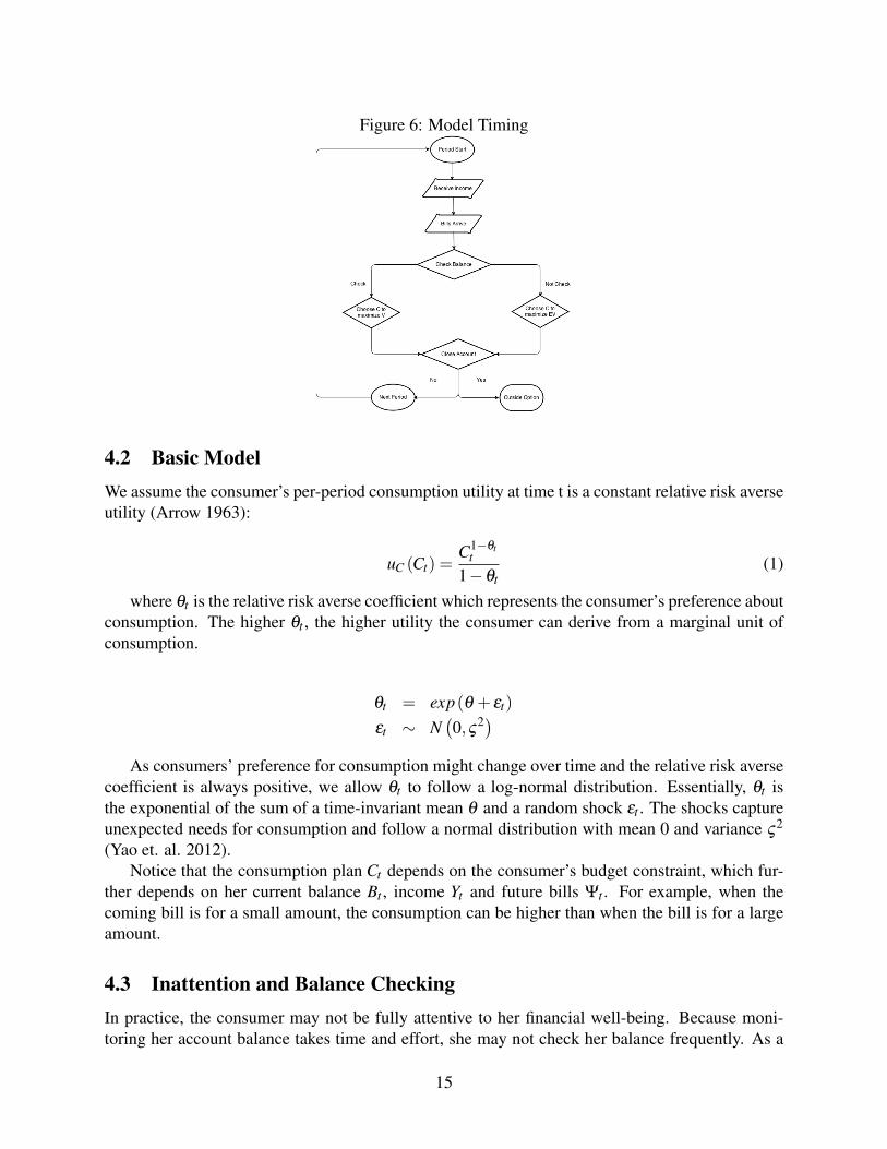
Figure 6: Model Timing

4.2 Basic ModelWe assume the consumer’s per-period consumption utility at time t is a constant relative risk averseutility (Arrow 1963):

uC (Ct) =C1−θt

t

1−θt(1)

where θt is the relative risk averse coefficient which represents the consumer’s preference aboutconsumption. The higher θt , the higher utility the consumer can derive from a marginal unit ofconsumption.

θt = exp(θ + εt)

εt ∼ N(0,ς2)

As consumers’ preference for consumption might change over time and the relative risk aversecoefficient is always positive, we allow θt to follow a log-normal distribution. Essentially, θt isthe exponential of the sum of a time-invariant mean θ and a random shock εt . The shocks captureunexpected needs for consumption and follow a normal distribution with mean 0 and variance ς2

(Yao et. al. 2012).Notice that the consumption plan Ct depends on the consumer’s budget constraint, which fur-

ther depends on her current balance Bt , income Yt and future bills Ψt . For example, when thecoming bill is for a small amount, the consumption can be higher than when the bill is for a largeamount.

4.3 Inattention and Balance CheckingIn practice, the consumer may not be fully attentive to her financial well-being. Because moni-toring her account balance takes time and effort, she may not check her balance frequently. As a

15

consequence, instead of knowing the exact (available) balance Bt12, she recalls a perceived bal-

ance Bt . Following Mehta, Rajiv and Srinivasan (2003), we allow the perceived balance Bt to bethe sum of the true balance Bt and a perception error ηtωt . The first component of the perceptionerror ηt is a random draw from the standard normal distribution13 and the second component is thestandard deviation of the perception error, ωt . So Bt follows a normal distribution

Bt ∼ N(Bt +ηtωt ,ω

2t)

The variance of the perception error ω2t measures the extent of uncertainty. Based on the

evidence from section 3.2.2, we allow this extent of uncertainty to accumulate through time whichimplies that the longer the consumer goes without checking her balance, the more inaccurate herperceived balance is. That is,

ω2t = ρΓt (2)

where Γt denotes the lapsed time since the consumer last checked her balance, and ρ denotes thesensitivity to lapsed time as shown in the equation (2) above14. Notice that the expected utility isdecreasing in the variance of the perception error ω2

t . This is true because the larger the varianceof the perception error, the less accurate the consumer’s estimate of her true balance, and the morelikely she is going to mistakenly overdraw, which lowers her utility.

We further assume that the consumer is sophisticated inattentive15 in the sense that she is awareof her own inattention (Grubb 2014). Sophisticated inattentive consumers are rational in that theychoose to be inattentive due to the high cost of monitoring her balances from day-to-day. Wealso model the consumer’s balance checking behavior. We denote the balance checking choice asQt ∈ 1,0 where 1 means check and 0 otherwise. If a consumer checks her balance, she incurs amonitoring cost but knows exactly what her balance is. So the perception error is reduced to zeroand she can make her optimal spending decision with all information. In mathematics form, herconsumption utility function changes to

ut =C1−θt

t

1−θt−Qtξ +χtQt (3)

where ξ is her balance checking cost and χQt is the idiosyncratic shock that affects her bal-ance checking cost. The shock χtQt can come from random events like a consumer checks balancebecause she’s also performing other types of transactions (like online bill payments) or she is onvacation without access to any bank channels so it’s hard for her to check balances. The equation

12Available balance means the initial balance plus income minus bills. For the ease of exposition, we omit the word"available" and only use "balance".

13The mean balance perception error η cannot be separately identified from the variance parameters ρ because theidentification sources both come from consumers’ overdraft fee payment. Specifically, the high overdraft payment fora consumer can be either explained by a positive balance perception error or large perception error variance caused bylarge ρ . So we fix η at zero, i.e. the perception error is assumed to be unbiased.

14We considered other specifications for the relationship between perception error variance and lapsed time sincelast balance check. Results remain qualitatively unchanged

15Consumers can also be naively inattentive, but we don’t allow it here. See discussion in Grubb 2014.

16

implies that if the consumer checks her balance, then her utility decreases by a monetary equiva-lence of [(1−θt)ξ ]

11−θt . We assume that χtQt are iid and follow a type I extreme value distribution.

If she doesn’t check, she recalls her balance Bt with the perception error ηt . So her perceivedbalance is

Bt ∼ QtBt +(1−Qt)N(Bt +ηtωt ,ω

2t)

She forms an expected utility based on her knowledge about the distribution of her perceptionerror. The optimal spending will maximize her “expected” utility after integrating out the balanceperception error, which is

ut =

ˆBt

ˆηt

ut

(Ct ; Bt

)dF (ηt)dF

(Bt

)4.4 Dissatisfaction and Account ClosingWe assume that the consumer also has the option of closing the account (e.g., an “outside option”).If she chooses to close the account, she might switch to other competing banks or become un-banked. With support from section 3.1, we make an assumption that consumers are sensitive to theratio of the overdraft fee to the overdraft transaction amount and we useΞit to denote this ratio asa state variable. We assume that the higher the ratio, the more likely it is that the consumer willbe dissatisfied to close the account because the forward-looking consumer anticipates that she’sgoing to accumulate more dissatisfaction (as well as lost consumption utility due to overdrafts) inthe future so that it’s not beneficial for her to keep the account open any more. Furthermore, weassume that consumers keep updating her belief of the ratio and only remembers the highest ratiothat has ever incurred. That is, if we use ∆t to denote the per-period ratio then

∆t =ODt

|Bt−Ct |

and

E [Ξt+1|Ξt ] = max(Ξt ,∆t)

This assumption reflects a consumer’s learning behavior over time in the sense that after experi-encing many overdrafts, a consumer realizes how costly (or dissatisfied) it could be for her to keepthe account open. When she learns that the ratio can be high enough so that it’s not beneficial forher to keep the account open any more, she’ll choose to close the account. Specifically, we add thedissatisfaction effect to the per-period utility function where

Ut = ut−ϒ∗∆t ∗ I[Bt−Ct < 0]

In the above equation, ut is defined in equation 3 and ϒ is the dissatisfaction sensitivity, i.e., theimpact of charging an overdraft fee on a consumer’s decision to close the account.

We assume that closing the account is a termination decison. Once a consumer chooses toclose the account, her value function (or total discounted utility function) equals an outside option

17

with a value normalized to 0 for identification purposes.16If the consumer keeps the account open,she’ll receive continution values from future per-period utility functions. More specifically, let Wdenote the choice to close the account, where W = 1 is closing the account and W = 0 is keepingthe account open. Then the value function for the consumer becomes

Vt =

Ut +ϖt0 +βE [Vt+1|St ] if Wt = 0Ut +ϖt1 if Wt = 1

where ϖt0 and ϖt1 are the idiosyncratic shocks that determine a consumer’s account closing de-cision. Sources of the shocks may include (1) the consumer moved address; (2) competing bankentered the market, and so on. We assume these shocks follow a type I extreme value distribution.

4.5 State Variables and the Transition ProcessWe have explained the following state variables in the model: (beginning) balance Bt , income Yt ,coming bill ψt , lapsed time since last balance check Γt , overdraft fee ODt , ratio of overdraft feeto the overdraft transaction amount Ξt , preference shock εt , balance checking cost shock χt andaccount closure utility shock ϖt . The other state variable to be introduced later, DLt , is involved inthe transition process.

For (available) balance Bt , the transition process satisfies the consumer’s budget constraint,which is

Bt+1 = Bt−Ct−ODt ∗ I (Bt−Ct < 0)+Yt+1−ψt+1

where ODt is the overdraft fee. As we model the consumer’s spending decision at the dailylevel rather than transaction level, we aggregate all overdraft fees paid and assume the consumerknows the per-item fee structure stated in section 3. This assumption is realistic in our setting be-cause we have already distinguished between inattentive and attentive consumers. The argumentthat a consumer might not be fully aware of the per-item fee is indirectly captured by the balanceperception error in the sense that the uncertain overdraft fee is equivalent to the uncertain balancebecause they both tighten the consumer’s budget constraint. As for the attentive consumer whooverdraws because of heavy discounting, she should be fully aware of the potential cost of over-draft. So in both cases we argue that the assumption of a known total overdraft fee is reasonable.

The state variable ODt is assumed to be iid over time and to follow a discrete distribution withsupport vector and probability vector X , p. The support vector contains multiples of the per-itemoverdraft fee.

Consistent with our data, we assume an income distribution as follows

Yt = Y ∗ I (DLt = PC)

where Y is the stable periodic (monthly/weekly/biweekly) income, DLt is the number of daysleft until the next payday and PC is the length of the pay cycle. The transition process of DL is

16Although the outside option is normalized to zero for all consumers, the implicit assumption is that we allow forheterogeneous utility of the outside option. The heterogeneity is reflected by the other structural parameters, includingthe dissatisfaction sensitivity.

18

deterministicDLt+1 = DLt−1+PC ∗ I (DLt = 1)

where it decreases by one for each period ahead and goes back to the full length when one paycycle ends.

The coming bills are assumed to be iid draws from a compound Poisson distribution with arrivalrate φ and jump size distribution G, Ψt ∼CP(φ ,G). This distribution can capture the pattern ofbills arriving randomly according to a Poisson process and bill sizes are sums of fixed components(each separate bill).

The time since last checking the balance also evolves deterministically based on the balancechecking behavior. Formally, we have

Γt+1 = 1+Γt (1−Qt)

which means that if the consumer checks her balance in the current period, then the lapsed timegoes back to 1 but if she doesn’t check, the lapsed time accumulates by one more period.

The ratio of the overdraft fee to the overdraft transaction amount evolves by keeping the maxi-mum amount over time.

E [Ξt+1|Ξt ] = max(Ξt ,∆t)

The shocks εt , χt and ϖt are all assumed to be iid over time.In summary, the whole state space for consumer is St =

Bt ,Ψt ,Yt ,DLt ,ODt ,Γt ,Ξt ,εt ,χt ,ϖt

.

In our dataset, we observe St = Bt ,ψt ,Yt ,DLt ,ODt ,Γt ,Ξt and our unobservable state variablesare St =

Bt ,ηt ,εt ,χt ,ϖt

. St = St ∪ St ∩Bt ,ψt. Notice here that consumers also have unob-

served states Bt and ψt due to inattention, which means that the consumer doesn’t know the truebalance (Bt) or the bill amount (ψt) if she doesn’t check her balance but only the perceived balance(Bt) and expected bill (Ψt).

4.6 The Dynamic Optimization Problem and Intertemporal TradeoffThe consumer chooses an infinite sequence of decision rules Ct ,Qt ,Wt∞

t=1in order to maximizethe expected total discounted utility:

maxCt ,Qt ,Wt∞

t=0

ESt∞

t=1

U0 (C0,Q0,W0;S0)+

∞

∑t=1

βtUt (Ct ,Qt ,Wt ;St) |S0

where

Ut (Ct ,Qt ,Wt ;St) =

[ˆBt

ˆηt

C1−θt

t

1−θt−Qtξ +χtQt

dF (ηt)dF

(Bt

)−ϒ

ODt ∗ I[Bt −Ct < 0]|Bt −Ct |

+ϖt0

](1−Wt)+Wtϖt1

.Let V (St) denote the value function:

V (St) = maxCτ ,Qτ ,Wτ∞

τ=t

ESτ∞

τ=t+1

Ut (St)+

∞

∑τ=t+1

βτ−tUτ (Sτ) |St

(4)

19

according to Bellman (1957), this infinite period dynamic optimization problem can be solvedthrough the Bellman Equation

V (St) = maxC,Q,W

ESt+1 U (C,Q,W ;St)+βV (St+1) |St (5)

In the infinite horizon dynamic programming problem, the policy function doesn’t depend ontime. So we can eliminate the time subscript. Then we have the following choice specific valuefunction:

v(C,Q,W ; B,Ψ,Y,DL,OD,Γ,Ξ,ε,χ,ϖ

)

=

uC (C)−ξ +χ1−ϒOD∗I[B−C<0]|B−C| +ϖ0

+βES+1

[V(

B+1,Ψ+1,Y+1,DL+1,OD+1,1,Ξ+1ε+1,χ+1,ϖ+1

)]if Q = 1&W = 0´

Bt

´ηt[uC (C)+χ0]dF (ηt)dF

(Bt

)−ϒ

OD∗I[B−C<0]|B−C| +ϖ0

+βES+1

[V(

B+1,Ψ+1,Y+1,DL+1,OD+1,Γ+1,Ξ+1,ε+1,χ+1,ϖ+1

)]if Q = 0&W = 0

ϖ1 if W = 1

(6)

where subscript+1 denotes the next time period. So the optimal policy is given by the followingsolution

C∗,Q∗,W ∗= argmaxv(C,Q,W ; B,Ψ,Y,DL,OD,Γ,Ξ,ε,χ,ϖ

)One thing that’s worth noticing is that there’s a distinction between this dynamic programming

problem and traditional ones. Because of the perception error, the consumer observes Bt = Bt +ηtωt but doesn’t know Bt or ηt . She only knows the distribution N(Bt +ηtωt ,ω

2t ). The consumer

makes a decision C∗(

Bt

)based on the perceived balance Bt . But as researchers, we don’t know the

realized perception error ηt . We observe the true balance Bt and the consumer’s spending C∗(

Bt

).

So we can only assume C∗(

Bt

)maximizes the “expected ex-ante value function”. Later we look

for parameters such that the likelihood for C∗(

Bt

)maximizes the expected ex-ante value function

attains maximum. Following Rust (1987), we obtain the ex-ante value function which integratesout the cost shocks, preference shocks, account closing shocks and unobserved mean balance error.

EV (B,ψ,Y,DL,OD,Γ,Ξ) =

ˆ

ϖ

ˆχ

ˆ

ε

ˆ

η

v(C∗,Q∗,W ∗; B,Ψ,Y,DL,OD,Γ,Ξ,ε,χ,ϖ

)dηdεdχdϖ

Consumers’ intertemporal trade-offs are associated with the three dynamic decisions. First ofall, given the budget constraint, a consumer will evaluate the utility of spending (or consuming)today versus tomorrow. The higher amount she spends today, the lower amount she can spendtomorrow. So spending is essentially a dynamic decision and the optimal choice for the consumeris to smooth out consumption over the time. Second, when deciding when to check balance, theconsumer will compare the monitoring cost with the expected gain from avoiding the overdraftfee. She’ll only check when the expected overdraft fee is higher than her monitoring cost. Asthe consumer’s balance perception error might accumulate with time, the consumer’s overdraft

20

probability also increases with the lapse time since the last balance check. As a result, the consumerwill wait until the overdraft probability reaches the certain threshold (when the expected overdraftfee equals the monitoring cost) to check the balance. Finally, the decision to close the account isan optimal stopping problem. The consumer will compare the total discounted utility of keepingthe account with the utility from the outside option to decide when to close the account. Whenexpecting too much overdraft fees as well as the accompanied dissatisfaction, the consumer willfind it more attractive to take the outside option and close the account.

4.7 HeterogeneityIn our data, consumers exhibit different responses to their state conditions. For example, someconsumers have never checked their balances and frequently overdraw while other consumersfrequently check their balances and rarely overdraw. We hypothesize that it’s due to their het-erogeneous discount factors and monitoring costs. Therefore, our model needs to account forunobserved heterogeneity. We follow a hierarchical Bayesian framework (Rossi, McCulloch andAllenby 2005) and incorporate heterogeneity by assuming that all parameters: βi (discount factor),ςi (standard deviation of risk averse coefficient),ξi (monitoring cost), ρi (sensitivity of error vari-ance to lapsed time since last checking balance) and ϒi (dissatisfaction sensitivity) have a randomcoefficient specification. For each of these parameters, ϑ ∈ βi,ςi,λi,ξi,ρi, the prior distributionis defined as ϑ ∼ N

(µϑ ,σ

2ϑ

). The hyper-prior distribution is assumed to be diffuse.

4.8 Numerical ExampleHere we use a numerical example to show that inattention can explain the observed overdraftoccasions in the data. More importantly, we display an interesting case in which an unbiasedperception can make the consumer spend less than the desired level. In this example, there aretwo periods, t ∈ 1,2. The consumer chooses the optimal consumption to maximize the expectedtotal discounted utility. In order to obtain an analytical solution for the optimal spending, weassume a CARA utility uC (Ct) =

1θ

exp(−θCt) and the coming bill following a normal distributionΨ2 ∼ N

(ψ2,ζ

22). The initial balance is B1 and the consumer receives income Y1 and Y2. As

period 2 is the termination period, the consumer will spend whatever is left from period 1, i.e.,C2 = B1 +Y1−ψ1−C1−OD ∗ (B1 +Y −ψ1−C1−ψ2)+Y2−ψ2. So the only decision is howmuch to spend for period 1: C1. Let θ = 0.07, B1 = 3.8, Y1 = 3, Y2 = 3, ψ2 = 1,ζ2 = 3.9,β = 0.99,OD = 3.58 (The values seem small compared to spending in reality because we apply log to allmonetary values).

21

4.8.1 Effect of Overdraft

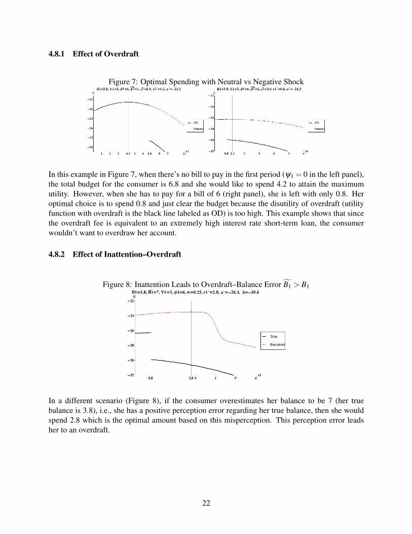
Figure 7: Optimal Spending with Neutral vs Negative Shock

In this example in Figure 7, when there’s no bill to pay in the first period (ψ1 = 0 in the left panel),the total budget for the consumer is 6.8 and she would like to spend 4.2 to attain the maximumutility. However, when she has to pay for a bill of 6 (right panel), she is left with only 0.8. Heroptimal choice is to spend 0.8 and just clear the budget because the disutility of overdraft (utilityfunction with overdraft is the black line labeled as OD) is too high. This example shows that sincethe overdraft fee is equivalent to an extremely high interest rate short-term loan, the consumerwouldn’t want to overdraw her account.

4.8.2 Effect of Inattention–Overdraft

Figure 8: Inattention Leads to Overdraft–Balance Error B1 > B1

In a different scenario (Figure 8), if the consumer overestimates her balance to be 7 (her truebalance is 3.8), i.e., she has a positive perception error regarding her true balance, then she wouldspend 2.8 which is the optimal amount based on this misperception. This perception error leadsher to an overdraft.

22

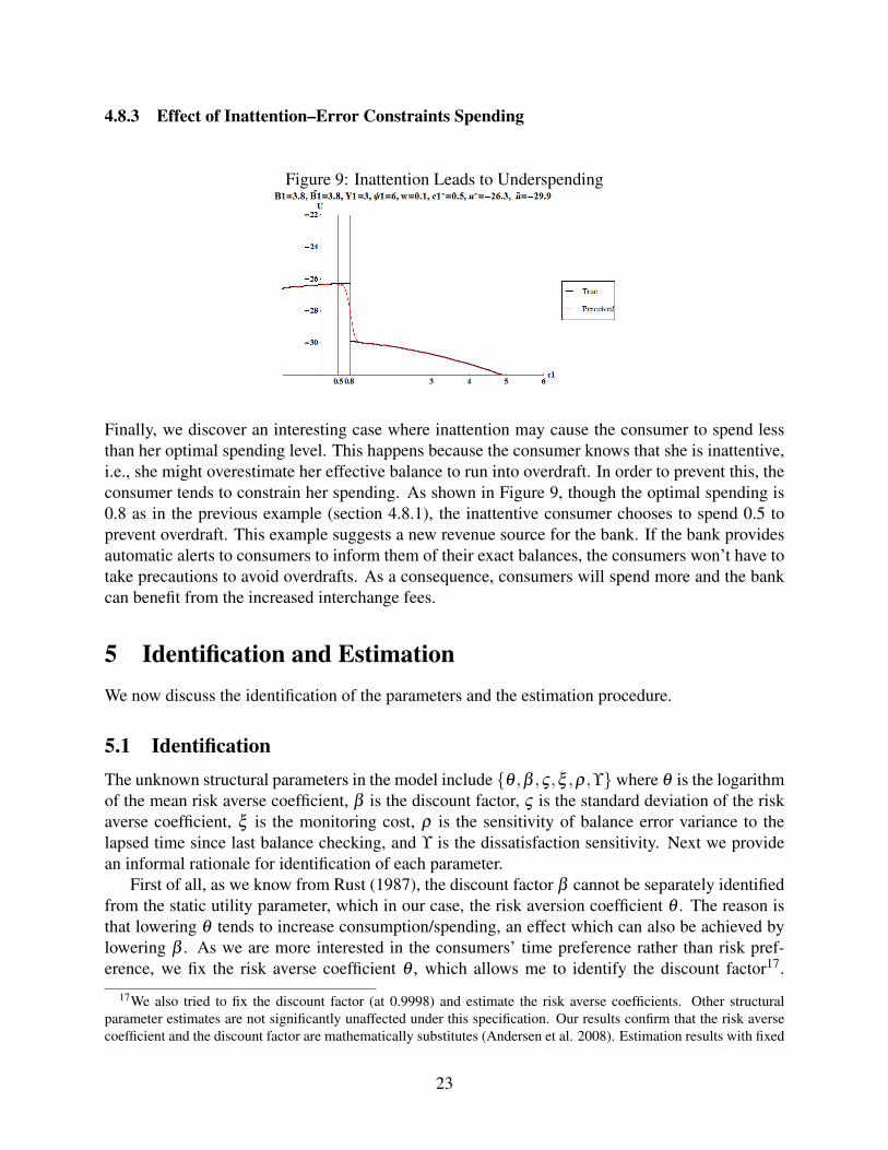
4.8.3 Effect of Inattention–Error Constraints Spending

Figure 9: Inattention Leads to Underspending

Finally, we discover an interesting case where inattention may cause the consumer to spend lessthan her optimal spending level. This happens because the consumer knows that she is inattentive,i.e., she might overestimate her effective balance to run into overdraft. In order to prevent this, theconsumer tends to constrain her spending. As shown in Figure 9, though the optimal spending is0.8 as in the previous example (section 4.8.1), the inattentive consumer chooses to spend 0.5 toprevent overdraft. This example suggests a new revenue source for the bank. If the bank providesautomatic alerts to consumers to inform them of their exact balances, the consumers won’t have totake precautions to avoid overdrafts. As a consequence, consumers will spend more and the bankcan benefit from the increased interchange fees.

5 Identification and EstimationWe now discuss the identification of the parameters and the estimation procedure.

5.1 IdentificationThe unknown structural parameters in the model include θ ,β ,ς ,ξ ,ρ,ϒwhere θ is the logarithmof the mean risk averse coefficient, β is the discount factor, ς is the standard deviation of the riskaverse coefficient, ξ is the monitoring cost, ρ is the sensitivity of balance error variance to thelapsed time since last balance checking, and ϒ is the dissatisfaction sensitivity. Next we providean informal rationale for identification of each parameter.

First of all, as we know from Rust (1987), the discount factor β cannot be separately identifiedfrom the static utility parameter, which in our case, the risk aversion coefficient θ . The reason isthat lowering θ tends to increase consumption/spending, an effect which can also be achieved bylowering β . As we are more interested in the consumers’ time preference rather than risk pref-erence, we fix the risk averse coefficient θ , which allows me to identify the discount factor17.

17We also tried to fix the discount factor (at 0.9998) and estimate the risk averse coefficients. Other structuralparameter estimates are not significantly unaffected under this specification. Our results confirm that the risk aversecoefficient and the discount factor are mathematically substitutes (Andersen et al. 2008). Estimation results with fixed

23

This practice is also used in Gopalakrishnan, Iyengar, Meyer 2014. As to the risk averse coeffi-cient, we choose θ = 0.74, following the latest literature by Andersen et al. (2008) where theyjointly elicit risk and time preferences18. After fixing θ , βi can be well identified by the sequencesof consumption (spending) within a pay period. A large discount factor (close to 1) implies astable consumption stream while a small discount factor implies a downward sloping consump-tion stream. Because a discount factor is constrained above by 1, we do a transformation to setβi =

11+exp(λi)

and estimate λi instead.Second, the standard deviation of risk averse coefficient ςi is identified by the variation of

consumptions on the same day of the pay period but across different pay periods.Moreover, according to the intertemporal tradeoff, the longer the consumer goes without check-

ing her balance, the more likely she will be to overdraw due to the balance error. The observeddata pattern of more overdraft fees paid longer after a balance checking inquiry can help pin downthe structural parameters ρi.

Intuitively, the monitoring cost ξi is identified by the expected overdraft payment amount.Recall that the tradeoff regarding balance checking is that a consumer only checks balance whenξi is smaller than the expected overdraft payment amount. In the data we observe the balancechecking frequency. Combining this with the calculated ρi we can compute the expected overdraftprobability and further the expected overdraft payment amount, which is the identified ξi. Givenρi, a consumer with few balance checking inquiries must have a higher balance checking cost ξi.

Lastly, the dissatisfaction sensitivity parameter ϒi can be identified by the data pattern thatconsumers’ account closure probability varies with the ratio of overdraft fee over the overdrafttransaction amount, as shown in section 3.1.

Note that aside from these structural parameters, there is another set of parameters that governthe transition process. These parameters can be identified prior to structural estimation from theobserved state variables in our data. The set includes φ ,G,X , p.

In sum, the structural parameters to be estimated include λi,ςi,ξi,ρi,ϒi.

5.2 LikelihoodThe full likelihood function is

L(

Cit ,Qit ,Wit ; SitT

t=1

I

i=1

)=

(L

Cit ,Qit ,Wit ; SitT

t=1

I

i=1

)L(

f

Sit |Sit−1T

t=1

I

i=1

)L(

Si0I

i=1

)where Sit = Bit ,ψit ,Yit ,DLit ,ODit ,Γit ,Ξt. As the likelihood for the optimal choices and that

for the state transition process are additively separable when we apply log to the likelihood func-tion, we can first estimate the state transition process from the data, then maximize the likelihoodfor the optimal choices. The likelihood function for the optimal choice is

discount factor are available upon requests.18We also tried other values for the relative risk averse coefficient θ , the estimated discount factor β values change

with different θ ’s, but other structural parameter values remain the same. The policy simulation results are also robustwith different values of θ ’s.

24

L(

Cit ,Qit ,Wit ; SitT

t=1

I

i=1

)=

L

∏i=1

T

∏t=1

L(Cit ; Sit

)L(Qit ; Sit

)L(Wit ; Sit

)=

L

∏i=1

T

∏t=1

f (εit |Cit)Pr (χit |Qit ,Cit)Pr (ϖit |Wit ,Qit ,Cit)

where f (εit |Cit) is estimated from the normal kernel density estimator to be explained in section5.3.1, Pr (χit |Cit ,Qit) and Pr (ϖit |Cit ,Qit ,Wit) follow the standard logit model given the choicespecific value function in equation 6. In specific,

Pr(Qit = 1; Sit

)=

ˆϖit

ˆεit

ˆηit

exp

v(Cit ,Qit = 1,Wit ; Sit

)∑Qit exp

v(Cit ,Qit ,Wit ; Sit

)Pr(Wit = 1; Sit

)=

ˆχit

ˆεit

ˆηit

exp

v(Cit ,Qit ,Wit = 1; Sit

)∑Wit exp

v(Cit ,Qit ,Wit ; Sit

)5.3 Estimation: Imai, Jain and Ching (2009)5.3.1 Modified IJC

We use the Bayesian estimation method developed by Imai, Jain and Ching (2009) to estimatethe dynamic choice problem with heterogeneous parameters. As our model involves a continuouschoice variable, spending, we adjust the IJC algorithm 19 to obtain the choice probability throughkernel density estimation. We now show the details of the estimation procedure. The whole param-eter space is divided into two sets (Ω= Ω1,Ω2), where the first one contains hyper-parameters inthe distribution of the heterogeneous parameters (Ω1 =

µλ ,µς ,µξ ,µρ ,µϒ,σλ ,σς ,σξ ,σρ ,σϒ

),

and the second set contains heterogeneous parameters (Ω2 = λi,ςi,ξi,ρi,ϒiIi=1) . We allow

all heterogeneous parameters (represented by ϑi) to follow a normal distribution with parametersmean µϑ and standard deviation σϑ . Let the observed choices be Od =

Od

iI

i=1 =

Cdi ,Q

di ,W

di

where Cdi ≡

Cd

it ,∀t

, Qdi ≡

Qd

it ,∀t

and W di ≡

W d

it ,∀t

.Each MCMC iteration mainly consists of two blocks.(i) Draw Ωr

1 , that is, draw µrϑ∼ fµϑ

(ϑ |σ r−1ϑ

,Ωr−12 ) and σ r

ϑ∼ fσϑ

(σϑ |µrϑ,Ωr−1

2 ) (ϑ ∈λ ,ς ,ξ ,ρ,ϒ,the parameters that capture the distribution of ϑ for the population) where fµϑ

and fσϑare the con-

ditional posterior distributions.(ii) Draw Ωr

2 , that is, draw individual parameters ϑi ∼ fi(ϑi|Od

i ,Ωr1)

by the Metropolis-Hastings (M-H) algorithm.

More details of the estimation algorithm is presented in Appendix A.2.

19The IJC method is designed for dynamic discrete choice problems. Zhou (2012) also applied it to a continuouschoice problem.

25

5.3.2 Parallel Computing: Neiswanger, Wang and Xing (2014)

We adopt the parallel computing algorithm by Neiswanger, Wang and Xing (2014) to estimate ourmodel with data from more than 500,000 consumers. The logic behind this algorithm is that thefull likelihood function is a multiplicative of the individual likelihood.

p(ϑ |xN)

∝ p(ϑ) p(xN |ϑ

)= p(ϑ)

N

∏i=1

p(xi|ϑ)

So we can partition the data onto multiple machines, and then perform MCMC sampling oneach using only the subset of data on that machine (in parallel, without any communication).Finally, we can combine the subposterior samples to algorithmically construct samples from thefull-data posterior.

In details, the procedure is:(1) Partition data xN into M subsets xn1 , ...,xnM.(2) For m = 1, ...,M (in parallel):(a) Sample from the subposterior pm, where pm (ϑ |xnm) ∝ p(ϑ)

1M p(xnm|ϑ)

(3) Combine the subposterior samples to produce samples from an estimate of the subposte-rior density product p1...pM, which is proportional to the full-data posterior, i.e. p1...pM (ϑ) ∝

p(ϑ |xN).Given T samples ϑtT

t=1 from a subposterior pm, we can write the kernel density estimator aspm (ϑ),

pm (ϑ) =1T

T

∑t=1

1hd K(

||ϑ −ϑt ||h

)

=1T

T

∑t=1

(2πh2)− d

2 |Id|−12 exp

− 1

2h2 (ϑ −ϑt)′ I−1

d (ϑ −ϑt)

=

1T

T

∑t=1

N(ϑ |ϑt ,h2Id

)where we have used a Gaussian kernel with bandwidth parameter h. After we have obtained the

kernel density estimator pm (ϑ) for M subposteriors, we define our nonparametric density productestimator for the full posterior as

p1 · · · pm (ϑ)

= p1 · · · pm (ϑ)

=1

T M

T

∑t1=1· · ·

T

∑tM=1

M

∏m=1

N(ϑ |ϑ m

tm ,h2Id)

∝T

∑t1=1· · ·

T

∑tM=1

N(

ϑ |ϑt·,h2

MId

) M

∏m=1

N(ϑ

mtm |ϑt·,h2Id

)∝

T

∑t1=1· · ·

T

∑tM=1

wt·N(

ϑ |ϑt·,h2

MId

)

26

This estimate is the probability density function (pdf) of a mixture of TM Gaussians withunnormalized mixture weights wt· Here, we use t·= t1, . . . , tM to denote the set of indices for theM samples

ϑ 1

t1, . . . ,ϑMtM

(each from one machine) associated with a given mixture component,

and let

wt· = N(

ϑ |ϑt·,h2

MId

)ϑt· =

1M

M

∑m=1

ϑmtm

(4) Given the hierarchical Bayes framework, after obtaining the posterior distribution of thepopulation parameter ϑ , use M-H algorithm once more to obtain the individual parameters (detailsin Appendix A.2 Step 4)

The sampling algorithm is presented in Appendix A.3.

6 Results

6.1 Model Comparison

Table 9: Model ComparisonA: No Forward Looking B: No Inattention C: No Heterogeneity D: Proposed

Log-Marginal Density -2943.28 -3636.59 -2764.56 -1758.33

Hit Rate: Overdraft 0.499 0.351 0.504 0.870

Hit Rate: Check Balance 0.405 0.226 0.632 0.841

Hit Rate: Close Account 0.660 0.727 0.696 0.758

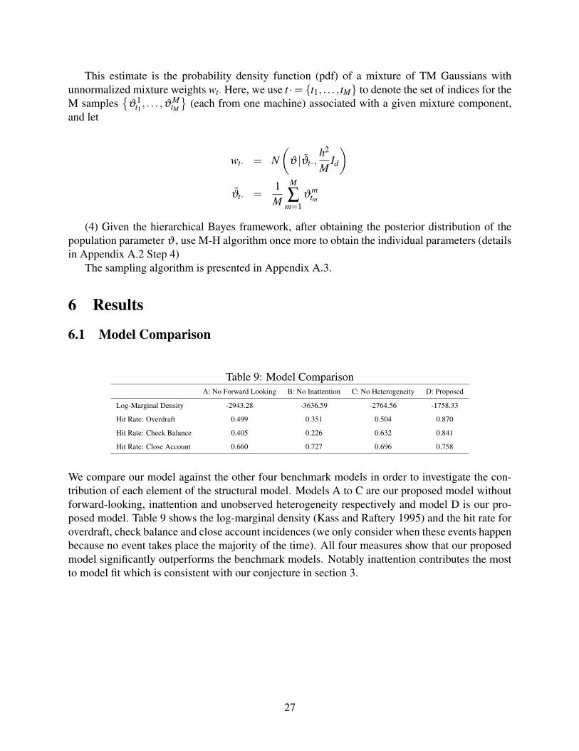
We compare our model against the other four benchmark models in order to investigate the con-tribution of each element of the structural model. Models A to C are our proposed model withoutforward-looking, inattention and unobserved heterogeneity respectively and model D is our pro-posed model. Table 9 shows the log-marginal density (Kass and Raftery 1995) and the hit rate foroverdraft, check balance and close account incidences (we only consider when these events happenbecause no event takes place the majority of the time). All four measures show that our proposedmodel significantly outperforms the benchmark models. Notably inattention contributes the mostto model fit which is consistent with our conjecture in section 3.

27

6.2 Value of Parallel IJC

Table 10: Estimation Time ComparisonSize\Method (seconds) Parallel IJC IJC CCP FIML

1,000 518 1579 526 5,01010,000 3,199 12,560 4,679 54,280

100,000 4,059 14,0813 55,226 640,360>500,000 5,308 788,294 399,337 3,372,660

(1.5 hr) (9 days) (5 days) (39 days)

Table 11: Monte Carlo Results when N=100,000Var True Value Parallel IJC IJC CCP FIML

µβ 0.9 Mean 0.878 0.883 0.851 0.892

Std 0.041 0.039 0.036 0.025

µς 1.5 Mean 1.505 1.502 1.508 1.501

Std 0.131 0.124 0.199 0.103

µξ 0.5 Mean 0.482 0.507 0.515 0.502

Std 0.056 0.039 0.071 0.044

µρ 1 Mean 1.006 1.003 1.015 1.002

Std 0.027 0.022 0.026 0.019

µϒ 5 Mean 5.032 5.011 4.943 4.987

Std 0.023 0.010 0.124 0.008

σβ 0.1 Mean 0.113 0.095 0.084 0.104

Std 0.016 0.014 0.015 0.010

σς 0.3 Mean 0.332 0.318 0.277 0.309

Std 0.024 0.015 0.029 0.021

σξ 0.1 Mean 0.112 0.091 0.080 0.090

Std 0.055 0.029 0.025 0.025

σρ 0.1 Mean 0.107 0.107 0.085 0.105

Std 0.008 0.006 0.010 0.006

σϒ 0.1 Mean 0.092 0.109 0.111 0.100

Std 0.014 0.013 0.021 0.009

We report the computational performance of different estimation methods in Table 10. All theexperiments are done on a server with an Intel Xeon CPU, 144 cores and 64 GB RAM. The firstcolumn is the performance of our proposed method, IJC with parallel computing. We compareit with the original IJC method, the Conditional Choice Probability (CCP) method by Arcidia-cono and Miller (2011) 20 and the Full Information Maximum Likelihood (FIML) method by Rust(1987) (or Nested Fixed Point Algorithm) 21. As the sample size increases, the comparative advan-

20We use the finite mixture model to capture unobserved heterogeneity and apply the EM algorithm to solve for theunobserved heterogeneity. More details of the estimation results can be obtained upon requests.

21We use the random coefficient model to capture unobserved heterogeneity. More details of the estimation resultscan be obtained upon requests.

28

tage of our proposed method is more notable. To run the model on the full dataset with more than500,000 accounts takes roughly 1.5 hours compared to 9 days with the original IJC method. Thereason for the decrease in computing time is that our method takes advantage of multiple machinesthat run in parallel. We further run a simulation study to see if the various methods are able toaccurately estimate all parameters. Table 11 shows that different methods produce quite similarestimates and all mean parameter estimates are within two standard errors of the true values. TheParallel IJC method is slightly less accurate than the original IJC method.

The parallel IJC is almost 600 times faster than FIML. This happens because the full solu-tion method solves the dynamic programming problem at each candidate value for the parameterestimates, whereas this IJC estimator only evaluates the value function once in each iteration.

6.3 Parameter Estimates

Table 12: Structural Model Estimation ResultsVar Interpretation Mean (µϑ ) Standard deviation (σϑ )βi Discount factor 0.9997 0.362

(0.00005) (0.058)ςi Standard deviation of relative risk aversion 0.257 0.028

(0.014) (0.003)ξi Monitoring cost 0.708 0.255

(0.084) (0.041)ρi Inattention Dynamics–lapsed time 7.865 0.648

(0.334) (0.097)ϒi Dissatisfaction Sensitivity 5.479 1.276

(1.329) (0.109)

Table 12 presents the results of the structural model. We find that the higher the age, the morerisk averse the consumer is. The monitoring cost is estimated to be 0.708. Using the risk aversecoefficient, we can evaluate the monitoring cost in monetary terms. It turns out to be $2.03. Wealso obtained the cost measure for each individual consumer.

The variance of the balance perception error increases with the lapsed time since the last timeto check balance and with the mean balance level. Notably the variance of the balance perceptionerror is quite large. If we take the average number of days to check the balance from the data,which is 9, then the standard deviation is 7.865 ∗ 9 = 70.79. This suggests a very widely spreaddistribution of the balance perception error.

The estimated dissatisfaction sensitivity parameter confirms our hypothesis that consumers canbe strongly affected by the bank fee and close the account as a consequence of dissatisfaction. If weconsider an average overdraft transaction amount at $33, then the relative magnitude of the effect ofdissatisfaction is comparable to $171. This suggests that unless the bank would like to offer a $171compensation to the consumer, the dissatisfied consumer will close the current account and switch.Moreover, consistent with the evidence in Figure 5, the dissatisfaction sensitivity is stronger forlight overdrafters (whose average is 5.911) than for heavy overdrafters (whose average is 3.387).

29

And keeping the average overdraft transaction amount as fixed, a 1% increase in the overdraft feecan increase the closing probability by 0.12%.

7 Counterfactuals

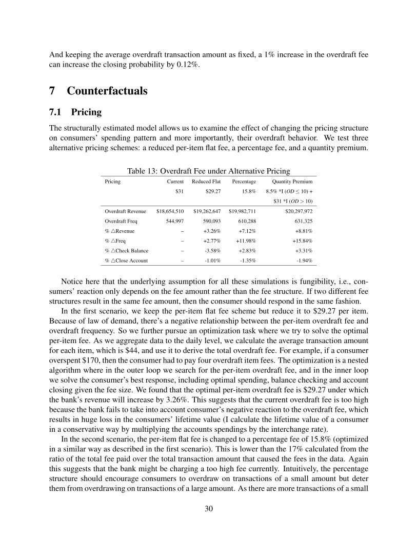
7.1 PricingThe structurally estimated model allows us to examine the effect of changing the pricing structureon consumers’ spending pattern and more importantly, their overdraft behavior. We test threealternative pricing schemes: a reduced per-item flat fee, a percentage fee, and a quantity premium.

Table 13: Overdraft Fee under Alternative PricingPricing Current Reduced Flat Percentage Quantity Premium

$31 $29.27 15.8% 8.5% *I (OD≤ 10) +

$31 *I (OD > 10)

Overdraft Revenue $18,654,510 $19,262,647 $19,982,711 $20,297,972

Overdraft Freq 544,997 590,093 610,288 631,325

%4Revenue – +3.26% +7.12% +8.81%

%4Freq – +2.77% +11.98% +15.84%

%4Check Balance – -3.58% +2.83% +3.31%

%4Close Account – -1.01% -1.35% -1.94%

Notice here that the underlying assumption for all these simulations is fungibility, i.e., con-sumers’ reaction only depends on the fee amount rather than the fee structure. If two different feestructures result in the same fee amount, then the consumer should respond in the same fashion.

In the first scenario, we keep the per-item flat fee scheme but reduce it to $29.27 per item.Because of law of demand, there’s a negative relationship between the per-item overdraft fee andoverdraft frequency. So we further pursue an optimization task where we try to solve the optimalper-item fee. As we aggregate data to the daily level, we calculate the average transaction amountfor each item, which is $44, and use it to derive the total overdraft fee. For example, if a consumeroverspent $170, then the consumer had to pay four overdraft item fees. The optimization is a nestedalgorithm where in the outer loop we search for the per-item overdraft fee, and in the inner loopwe solve the consumer’s best response, including optimal spending, balance checking and accountclosing given the fee size. We found that the optimal per-item overdraft fee is $29.27 under whichthe bank’s revenue will increase by 3.26%. This suggests that the current overdraft fee is too highbecause the bank fails to take into account consumer’s negative reaction to the overdraft fee, whichresults in huge loss in the consumers’ lifetime value (I calculate the lifetime value of a consumerin a conservative way by multiplying the accounts spendings by the interchange rate).

In the second scenario, the per-item flat fee is changed to a percentage fee of 15.8% (optimizedin a similar way as described in the first scenario). This is lower than the 17% calculated from theratio of the total fee paid over the total transaction amount that caused the fees in the data. Againthis suggests that the bank might be charging a too high fee currently. Intuitively, the percentagestructure should encourage consumers to overdraw on transactions of a small amount but deterthem from overdrawing on transactions of a large amount. As there are more transactions of a small

30

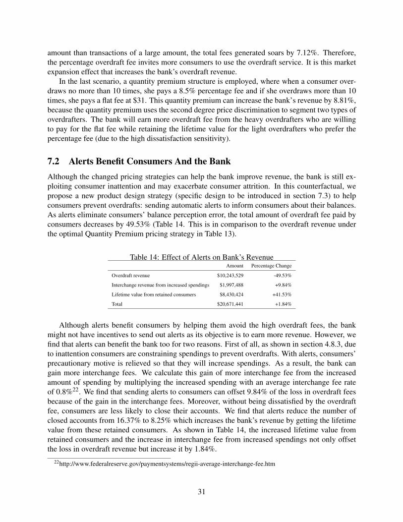
amount than transactions of a large amount, the total fees generated soars by 7.12%. Therefore,the percentage overdraft fee invites more consumers to use the overdraft service. It is this marketexpansion effect that increases the bank’s overdraft revenue.

In the last scenario, a quantity premium structure is employed, where when a consumer over-draws no more than 10 times, she pays a 8.5% percentage fee and if she overdraws more than 10times, she pays a flat fee at $31. This quantity premium can increase the bank’s revenue by 8.81%,because the quantity premium uses the second degree price discrimination to segment two types ofoverdrafters. The bank will earn more overdraft fee from the heavy overdrafters who are willingto pay for the flat fee while retaining the lifetime value for the light overdrafters who prefer thepercentage fee (due to the high dissatisfaction sensitivity).

7.2 Alerts Benefit Consumers And the BankAlthough the changed pricing strategies can help the bank improve revenue, the bank is still ex-ploiting consumer inattention and may exacerbate consumer attrition. In this counterfactual, wepropose a new product design strategy (specific design to be introduced in section 7.3) to helpconsumers prevent overdrafts: sending automatic alerts to inform consumers about their balances.As alerts eliminate consumers’ balance perception error, the total amount of overdraft fee paid byconsumers decreases by 49.53% (Table 14. This is in comparison to the overdraft revenue underthe optimal Quantity Premium pricing strategy in Table 13).

Table 14: Effect of Alerts on Bank’s RevenueAmount Percentage Change

Overdraft revenue $10,243,529 -49.53%

Interchange revenue from increased spendings $1,997,488 +9.84%

Lifetime value from retained consumers $8,430,424 +41.53%

Total $20,671,441 +1.84%

Although alerts benefit consumers by helping them avoid the high overdraft fees, the bankmight not have incentives to send out alerts as its objective is to earn more revenue. However, wefind that alerts can benefit the bank too for two reasons. First of all, as shown in section 4.8.3, dueto inattention consumers are constraining spendings to prevent overdrafts. With alerts, consumers’precautionary motive is relieved so that they will increase spendings. As a result, the bank cangain more interchange fees. We calculate this gain of more interchange fee from the increasedamount of spending by multiplying the increased spending with an average interchange fee rateof 0.8%22. We find that sending alerts to consumers can offset 9.84% of the loss in overdraft feesbecause of the gain in the interchange fees. Moreover, without being dissatisfied by the overdraftfee, consumers are less likely to close their accounts. We find that alerts reduce the number ofclosed accounts from 16.37% to 8.25% which increases the bank’s revenue by getting the lifetimevalue from these retained consumers. As shown in Table 14, the increased lifetime value fromretained consumers and the increase in interchange fee from increased spendings not only offsetthe loss in overdraft revenue but increase it by 1.84%.

22http://www.federalreserve.gov/paymentsystems/regii-average-interchange-fee.htm

31

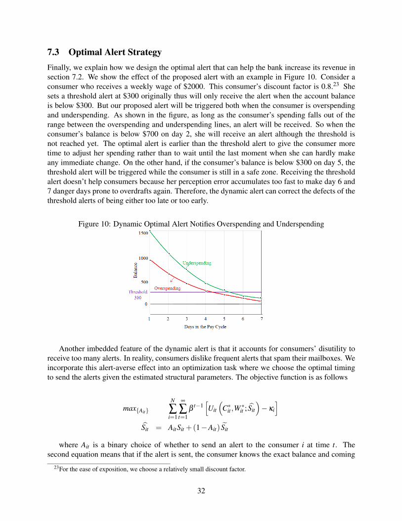
7.3 Optimal Alert StrategyFinally, we explain how we design the optimal alert that can help the bank increase its revenue insection 7.2. We show the effect of the proposed alert with an example in Figure 10. Consider aconsumer who receives a weekly wage of $2000. This consumer’s discount factor is 0.8.23 Shesets a threshold alert at $300 originally thus will only receive the alert when the account balanceis below $300. But our proposed alert will be triggered both when the consumer is overspendingand underspending. As shown in the figure, as long as the consumer’s spending falls out of therange between the overspending and underspending lines, an alert will be received. So when theconsumer’s balance is below $700 on day 2, she will receive an alert although the threshold isnot reached yet. The optimal alert is earlier than the threshold alert to give the consumer moretime to adjust her spending rather than to wait until the last moment when she can hardly makeany immediate change. On the other hand, if the consumer’s balance is below $300 on day 5, thethreshold alert will be triggered while the consumer is still in a safe zone. Receiving the thresholdalert doesn’t help consumers because her perception error accumulates too fast to make day 6 and7 danger days prone to overdrafts again. Therefore, the dynamic alert can correct the defects of thethreshold alerts of being either too late or too early.

Figure 10: Dynamic Optimal Alert Notifies Overspending and Underspending

Another imbedded feature of the dynamic alert is that it accounts for consumers’ disutility toreceive too many alerts. In reality, consumers dislike frequent alerts that spam their mailboxes. Weincorporate this alert-averse effect into an optimization task where we choose the optimal timingto send the alerts given the estimated structural parameters. The objective function is as follows

maxAit

N

∑i=1

∞

∑t=1

βt−1[Uit

(C∗it ,W

∗it ; Sit

)−κi

]Sit = AitSit +(1−Ait) Sit

where Ait is a binary choice of whether to send an alert to the consumer i at time t. Thesecond equation means that if the alert is sent, the consumer knows the exact balance and coming

23For the ease of exposition, we choose a relatively small discount factor.

32

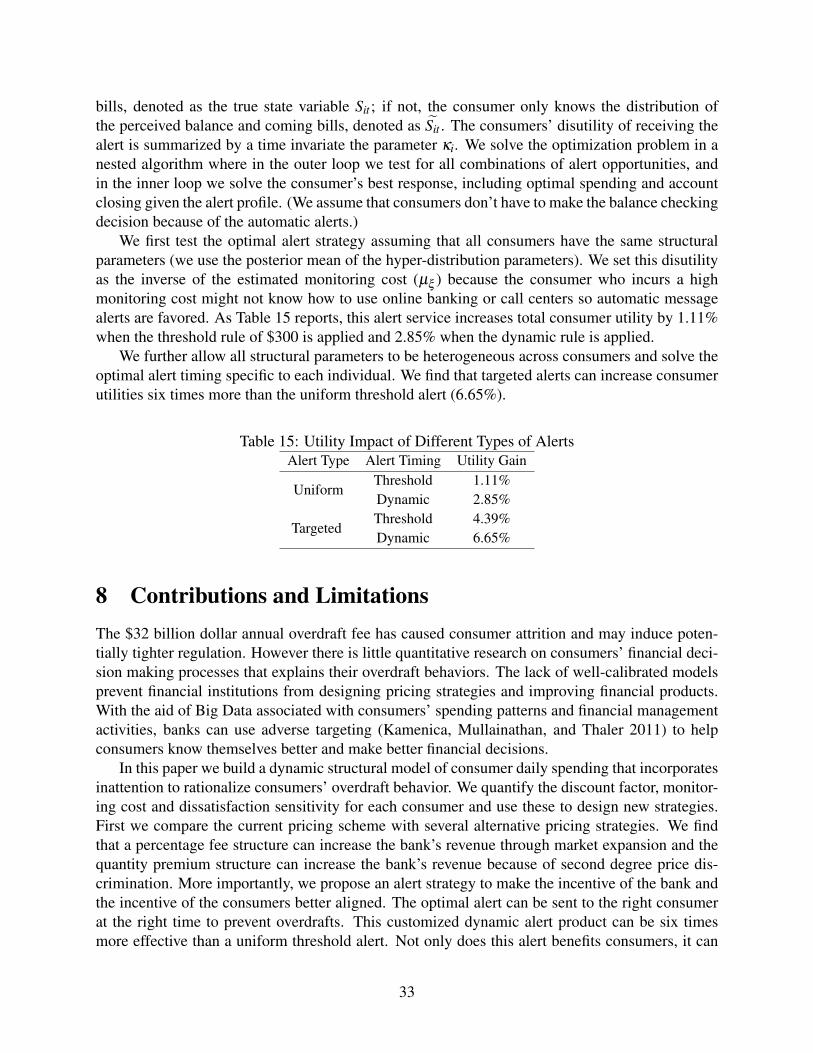
bills, denoted as the true state variable Sit ; if not, the consumer only knows the distribution ofthe perceived balance and coming bills, denoted as Sit . The consumers’ disutility of receiving thealert is summarized by a time invariate the parameter κi. We solve the optimization problem in anested algorithm where in the outer loop we test for all combinations of alert opportunities, andin the inner loop we solve the consumer’s best response, including optimal spending and accountclosing given the alert profile. (We assume that consumers don’t have to make the balance checkingdecision because of the automatic alerts.)

We first test the optimal alert strategy assuming that all consumers have the same structuralparameters (we use the posterior mean of the hyper-distribution parameters). We set this disutilityas the inverse of the estimated monitoring cost (µξ ) because the consumer who incurs a highmonitoring cost might not know how to use online banking or call centers so automatic messagealerts are favored. As Table 15 reports, this alert service increases total consumer utility by 1.11%when the threshold rule of $300 is applied and 2.85% when the dynamic rule is applied.

We further allow all structural parameters to be heterogeneous across consumers and solve theoptimal alert timing specific to each individual. We find that targeted alerts can increase consumerutilities six times more than the uniform threshold alert (6.65%).

Table 15: Utility Impact of Different Types of AlertsAlert Type Alert Timing Utility Gain

UniformThreshold 1.11%Dynamic 2.85%

TargetedThreshold 4.39%Dynamic 6.65%

8 Contributions and LimitationsThe $32 billion dollar annual overdraft fee has caused consumer attrition and may induce poten-tially tighter regulation. However there is little quantitative research on consumers’ financial deci-sion making processes that explains their overdraft behaviors. The lack of well-calibrated modelsprevent financial institutions from designing pricing strategies and improving financial products.With the aid of Big Data associated with consumers’ spending patterns and financial managementactivities, banks can use adverse targeting (Kamenica, Mullainathan, and Thaler 2011) to helpconsumers know themselves better and make better financial decisions.

In this paper we build a dynamic structural model of consumer daily spending that incorporatesinattention to rationalize consumers’ overdraft behavior. We quantify the discount factor, monitor-ing cost and dissatisfaction sensitivity for each consumer and use these to design new strategies.First we compare the current pricing scheme with several alternative pricing strategies. We findthat a percentage fee structure can increase the bank’s revenue through market expansion and thequantity premium structure can increase the bank’s revenue because of second degree price dis-crimination. More importantly, we propose an alert strategy to make the incentive of the bank andthe incentive of the consumers better aligned. The optimal alert can be sent to the right consumerat the right time to prevent overdrafts. This customized dynamic alert product can be six timesmore effective than a uniform threshold alert. Not only does this alert benefits consumers, it can

33

also benefit the bank through increased interchange fees and lower consumer attrition.We calibrated our model at an individual level on a sample of more than 500,000 accounts.

This Big Data provide great value for our analysis. First of all, an overdraft is still a relativelyrare event compared to numerous other transactions. Without a large amount of data, we cannotdetect these rare but detrimental events, let alone their diverse causes. Second, as summarized byEinav and Levin (2014), Big Data contain rich micro-level variation that can used to identify novelbehavior and develop predictive models that are harder with smaller samples, fewer variables, andmore aggregation. We leverage the variation in consumer daily spending and balance checkingbehaviors to evaluate the effect of heterogeneous policy instruments. These evaluations can beuseful for bank managers to design new products and policy makers to create new regulation rulesat a much more refined fashion than before.

In order to estimate a complicated structural model with Big Data, we adopt parallel computingtechniques in combination with the Bayesian estimation algorithm developed by Imai, Jain andChing (2009). This new method significantly reduces the computation burden and could be usedfor other researchers and marketers who would like to use structural models to solve real-worldlarge-scale problems.

There are several limitations of the current study that call for future work. First, we don’tobserve consumers’ existing alert settings. Some consumers may have already received alertsto help them make financial decisions. In our policy simulations, we made bold assumptionsabout consumers’ disutility for reading alerts. These assumptions could be tested if we had thealerts data. The current alerts are set by consumers who might fail to consider their spendingdynamics. Future field experiments are needed to test the effect of our proposed alert strategy.Second, we don’t have the data about consumers’ decision on whether to opt-in for overdraftprotection by ATM/POS transactions. We only know that if ATM/POS transactions caused anoverdraft, then the consumer must have opted-in. If no such transactions happened, we do notknow the consumer’s opt-in status. Had we known this information, we could have providedan informative prior in our the Bayesian model. The logic is that a consumer who has opted inprobably has stronger needs for short term liquidity due to fluctuations in the size and arrival timeof income and expenditures. Finally, we only model consumers’ non-preauthorized spending in thechecking account. In reality, consumers usually have multiple accounts, like savings, credit cardsand loans, with multiple financial institutions. A model to capture consumers’ decisions acrossall accounts for both short-term and long-term finances will provide a more complete picture ofconsumers’ financial management capabilities and resources so that the bank can design morecustomized products.

ReferencesAndersen, S., Harrison, G. W., Lau, M. I., & Rutström, E. E. (2008). Eliciting risk and timepreferences. Econometrica, 76(3), 583-618.Arcidiacono, P., & Miller, R. A. (2011). Conditional choice probability estimation of dynamicdiscrete choice models with unobserved heterogeneity. Econometrica, 79(6), 1823-1867.Arrow, K. J. 1963. Liquidity preference. Lecture VI in Lecture Notes for Economics 285, TheEconomics of Uncertainty, pp. 33-53, undated, Stanford University.Bellman, Richard 1957. Dynamic Programming, Princeton, NJ: Princeton University Press.

34

Bolton, R. N. (1998). A dynamic model of the duration of the customer’s relationship with acontinuous service provider: the role of satisfaction. Marketing science, 17(1), 45-65.Chetty, R., Looney, A., & Kroft, K. (2009). Salience and taxation: Theory and evidence. AmericanEconomic Review, 99(4), 1145-1177.Card, D., DellaVigna, S., & Malmendier, U. (2011). The role of theory in field experiments. TheJournal of Economic Perspectives, 25(3), 39-62.Einav, L., & Levin, J. D. (2014). The data revolution and economic analysis. Innovation Policyand the Economy, forthcoming.Evans, D., Litan, R., & Schmalensee, R. (2011). Economic Analysis of the Effects of the Fed-eral Reserve Board’s Proposed Debit Card Interchange Fee Regulations on Consumers and SmallBusinesses. Available at SSRN 1769887.Fang, H., & Silverman, D. (2009). Time-inconsistency and welfare program participation: Evi-dence from the nlsy. International Economic Review, 50(4), 1043-1077.Fishman, M. J., & Hagerty, K. M. (2003). Mandatory versus voluntary disclosure in markets withinformed and uninformed customers. Journal of Law, Economics, and Organization, 19(1), 45-63.Gabaix, X., & Laibson, D. (2006). Shrouded attributes, consumer myopia, and information sup-pression in competitive markets. The Quarterly Journal of Economics, 121(2), 505-540.Gopalakrishnan, A., Iyengar, R., & Meyer, R. J. (2014). Consumer dynamic usage allocation andlearning under multi-part tariffs: theory and empirical evidence. Working paper, Wharton School,University of Pennsylvania.Grubb, M. D. (2014). Consumer inattention and bill-shock regulation. The Review of EconomicStudies, forthcoming.Grubb, M. D., & Osborne, M. (2014) Cellular Service Demand: Biased Beliefs, Learning, and BillShock. American Economic Review, forthcoming.Haselhuhn, M. P., Pope, D. G., Schweitzer, M. E., & Fishman, P. (2012). The impact of personalexperience on behavior: Evidence from video-rental fines. Management Science, 58(1), 52-61.Hirshleifer, D., & Hong Teoh, S. (2003). Herd behaviour and cascading in capital markets: Areview and synthesis. European Financial Management, 9(1), 25-66.Imai, S., Jain, N., & Ching, A. (2009). Bayesian estimation of dynamic discrete choice models.Econometrica, 77(6), 1865-1899.Jiang, L. (2012). The welfare effects of "bill shock" regulation in mobile telecommunication mar-kets. Working Paper, University of British Columbia.Kahneman, D., J. Knetsch, and R. Thaler (1990). Experimental Tests of the Endowment Effectand the Coase Theorem. Journal of Political Economy, 98(6), 1325–1348.Kahneman, D., & Tversky, A. (1979). Prospect theory: An analysis of decision under risk. Econo-metrica: Journal of the Econometric Society, 263-291.Kamenica, E., Mullainathan, S., & Thaler, R. (2011). Helping consumers know themselves. TheAmerican Economic Review, 101(3), 417-422.Karlan, D., McConnell, M., Mullainathan, S., & Zinman, J. (2010). Getting to the top of mind:How reminders increase saving (No. w16205). National Bureau of Economic Research.Kass, R., and A. Raftery. (1995). Bayes Factors. Journal of the American Statistical Association90 (430): 773-95.Keaveney, S. M. (1995). Customer switching behavior in service industries: an exploratory study.The Journal of Marketing, 71-82.

35

Magnac, T., & Thesmar, D. (2002). Identifying dynamic discrete decision processes. Economet-rica, 70(2), 801-816.Matzler, K., Würtele, A., & Renzl, B. (2006). Dimensions of price satisfaction: a study in the retailbanking industry. International Journal of Bank Marketing, 24(4), 216-231.Mehta, N., Rajiv, S., & Srinivasan, K. (2003). Price uncertainty and consumer search: A structuralmodel of consideration set formation. Marketing science, 22(1), 58-84.Neiswanger, W., Wang, C., & Xing, E. (2014). Asymptotically exact, embarrassingly parallelMCMC. Proceedings of the 30th International Conference on Conference on Uncertainty in Arti-ficial Intelligence.Peng, L., & Xiong, W. (2006). Investor attention, overconfidence and category learning. Journalof Financial Economics, 80(3), 563-602.Pope, D. G. (2009). Reacting to rankings: Evidence from “America’s Best Hospitals”. Journal ofHealth Economics, 28(6), 1154-1165.Rossi, Peter E., Allenby, G. M., & McCulloch, R. E. (2005). Bayesian statistics and marketing. J.Wiley & Sons.Rust, J. (1987). Optimal replacement of GMC bus engines: An empirical model of Harold Zurcher.Econometrica: Journal of the Econometric Society, 999-1033.Stango, V., & Zinman, J. (2014). Limited and varying consumer attention: Evidence from shocksto the salience of bank overdraft fees. Review of Financial Studies, forthcoming.Yao, S., Mela, C. F., Chiang, J., & Chen, Y. (2012). Determining consumers’ discount rates withfield studies. Journal of Marketing Research, 49(6), 822-841.Zhou, Y. (2012). Failure to Launch in Two-Sided Markets: A Study of the US Video Game Market.Working paper, SUNY at Stony Brook.

36

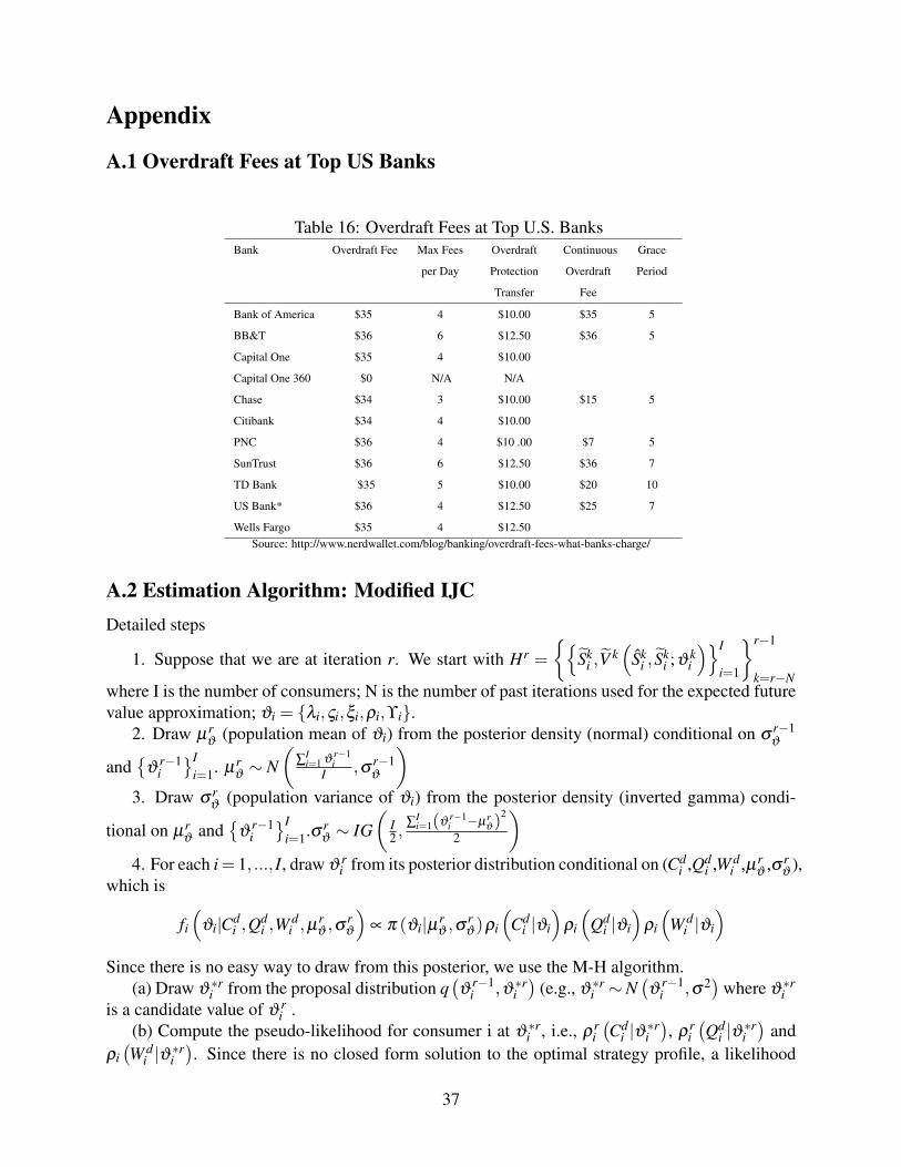
Appendix

A.1 Overdraft Fees at Top US Banks

Table 16: Overdraft Fees at Top U.S. BanksBank Overdraft Fee Max Fees

per Day

Overdraft

Protection

Transfer

Continuous

Overdraft

Fee

Grace

Period

Bank of America $35 4 $10.00 $35 5

BB&T $36 6 $12.50 $36 5

Capital One $35 4 $10.00

Capital One 360 $0 N/A N/A

Chase $34 3 $10.00 $15 5

Citibank $34 4 $10.00

PNC $36 4 $10 .00 $7 5

SunTrust $36 6 $12.50 $36 7

TD Bank $35 5 $10.00 $20 10

US Bank* $36 4 $12.50 $25 7

Wells Fargo $35 4 $12.50Source: http://www.nerdwallet.com/blog/banking/overdraft-fees-what-banks-charge/

A.2 Estimation Algorithm: Modified IJCDetailed steps

1. Suppose that we are at iteration r. We start with Hr =

Sk

i ,Vk(

Ski , S

ki ;ϑ k

i

)I

i=1

r−1

k=r−Nwhere I is the number of consumers; N is the number of past iterations used for the expected futurevalue approximation; ϑi = λi,ςi,ξi,ρi,ϒi.

2. Draw µrϑ

(population mean of ϑi) from the posterior density (normal) conditional on σr−1ϑ

and

ϑr−1iI

i=1. µrϑ∼ N

(∑

Ii=1 ϑ

r−1i

I ,σ r−1ϑ

)3. Draw σ r

ϑ(population variance of ϑi) from the posterior density (inverted gamma) condi-

tional on µrϑ

and

ϑr−1iI

i=1.σ rϑ∼ IG

(I2 ,

∑Ii=1(ϑ

r−1i −µr

ϑ)2

2

)4. For each i= 1, ..., I, draw ϑ r

i from its posterior distribution conditional on (Cdi ,Qd

i ,W di ,µr

ϑ,σ r

ϑ),

which is

fi

(ϑi|Cd

i ,Qdi ,W

di ,µ

rϑ ,σ

rϑ

)∝ π (ϑi|µr

ϑ ,σrϑ )ρi

(Cd

i |ϑi

)ρi

(Qd

i |ϑi

)ρi

(W d

i |ϑi

)Since there is no easy way to draw from this posterior, we use the M-H algorithm.

(a) Draw ϑ ∗ri from the proposal distribution q(ϑ

r−1i ,ϑ ∗ri

)(e.g., ϑ ∗ri ∼N

(ϑ

r−1i ,σ2)where ϑ ∗ri

is a candidate value of ϑ ri .

(b) Compute the pseudo-likelihood for consumer i at ϑ ∗ri , i.e., ρri(Cd

i |ϑ ∗ri), ρr

i(Qd

i |ϑ ∗ri)

andρi(W d

i |ϑ ∗ri). Since there is no closed form solution to the optimal strategy profile, a likelihood

37

function based on observed Cit becomes infeasible. Instead, we implement a numerical approxi-mation method to establish a simulated likelihood function for estimation. For each Cit observedin the data and its corresponding state point Sit , we use the following steps to simulate its density:

i. First assume the unobserved state variables are Sit = εit ,ηit ,χit ,ϖit. Draw nr=1000 randomshocks Sit = εit ,ηit ,χit ,ϖit from

ηit ∼ N(0,ω2i ), εit ∼ N (0,1),χit~EVI

24,ϖit~EVI;

i. For each balance checking decision Q = 1,0and account closing decision W = 1,0, eachrandom draw of Sit and the observed Sit , calculate the optimal consumption by solving the follow-ing equations

C∗it(

Sit , Sit |Q,W)

= argmaxCit

vr(

Q,W ; Sit , Sit ,ϑ∗ri

)= argmax

CitU(

Cit ,Q,W ; Sit , Sit ,ϑ∗ri

)+β Er

Sit+1

V(

Sit+1, Sit+1;ϑ∗ri

)|Sit , Sit

iii. Using the calculated nr = 1000 optimal C∗it(

Sit , Sit

), simulate ρr

i(Cd

it |ϑ ∗ri), the density of

the observed Cdit , using a Gaussian kernel density estimator. (This simulation borrows an idea from

Yao, Mela, Chiang and Chen (2012)) . Moreover,

ρi

(Qd

it |ϑ ∗ri

)=

1nr ∑

η ,ε,ϖ

exp

vχit

(C∗it ,Q = Qit ,W ∗it ; Bit ,Rit ,Ψit ,Yit ,DLit ,Dit ,ODit ,Γit ,Ξit ,εit ,ϖit ,ϑ

∗ri

)∑Q∈1,0 exp

vχit

(C∗it ,Q,W ∗it ; Bit ,Rt ,Ψit ,Yit ,DLit ,Dit ,ODit ,Γit ,Ξit ,εit ,ϖit ,ϑ ∗ri

)and

ρi

(W d

it |ϑ ∗ri

)=

1nr ∑

η ,ε,χ

exp

vϖ

(C∗it ,Q

∗it ,W =Wit ; Bit ,Rit ,Ψit ,Yit ,DLit ,Dit ,ODit ,Γit ,Ξit ,εit ,χit ,ϑ

∗ri

)∑W∈1,0 exp

vϖ

(C∗it ,Q

∗it ,W ; Bit ,Rt ,Ψit ,Yit ,DLit ,Dit ,ODit ,Γit ,Ξit ,εit ,χit ,ϑ ∗ri

)ρi

(Od

i |ϑ ∗ri

)= ρi

(Cd

i |ϑ ∗ri

)ρi

(Qd

i |ϑ ∗ri

)ρi

(W d

i |ϑ ∗ri

)=

T

∏t=1

ρi

(Cd

it |ϑ ∗ri

)ρi

(Qd

it |ϑ ∗ri

)ρi

(W d

it |ϑ ∗ri

).

To obtain vr(

Sit , Sit ,ϑ∗ri

), we need Er

S′

V(

S′i, S′i;ϑ ∗ri

)|Si, Si

, which is obtained by a weighted

average of

V k(

Ski , S

ki ;ϑ ∗ki

)r−1

k=r−N, treating ϑi as one of the parameters when computing the

weights. In the case of independent kernels, for all Si = Bi,ψi,Yi,DLi,ODi,Γi,Ξi, because Bi,Ξiare continuous and evolves deterministically, ψi and ODi are continuous and evolve stochastically,and Yi,DLi,Γi are discrete so

ErS′

V(

B′i,ψ′i ,Y′i ,DL′i,OD′i,Γ

′i,Ξ′i, S′i;ϑ∗ri

)|Bi,ψi,Yi,DLi,ODi,Γi,Ξi, Si

=

r−1

∑k=r−N

V k(

Bki ,ψ

ki ,Y′i ,DL′i,ODk

i ,Γ′i,Ξ′i, S

ki ;ϑ

∗ki

) Khϑ

(ϑ ∗ri −ϑ ∗ki

)Khs(B′i−Bk

i)

f(ψk

i |φi,Gi)

f(ODk

i |Xi, pi)

Khs(Ξ′i−Ξk

i)

∑r−1l=r−N Khϑ

(ϑ ∗ri −ϑ ∗li

)Khs(B′i−Bl

i)

f(ψ l

i |φi,Gi)

f(ODl

i |Xi, pi)

Khs(Ξ′i−Ξl

i)

We repeat the same step and obtain the pseudo-likelihood (ρri(Od

i |ϑr−1i)) conditional on

(ϑ

r−1i).

Then, we determine whether or not to accept ϑ ∗ri . The acceptance probability, Λ, is given by

Λ = min

(π(ϑ ∗ri |µr

ϑ,σ r

ϑ

)ρr

i(Od

i |ϑ ∗ri)

q(ϑ ∗ri ,ϑ r−1

i)

π(ϑ

r−1i |µr

ϑ,σ r

ϑ

)ρr

i(Od

i |ϑr−1i)

q(ϑ

r−1i ,ϑ ∗ri

) ,1)24Type I Extreme Value Distribution

38

where π (·) denotes the prior distribution.(c) Repeat (a) & (b) for all i.

5. Computation of the pseudo-value function,

V r(

Sri , S

ri ;ϑ ∗ri

)I

i=1(a) Make one draw of the unobserved state variables Sr

i from ηi∼N(0,ω2i ), εi∼N

(0,ς2

i),χi~EVI25,

and ϖi~EVI;(b) Compute the pseudo expected future value at ϑ ∗ri .

ErS′i

V(

S′i, S′i;ϑ∗ri

)|Sr

i , Sri

=

r−1

∑k=r−N

V k(

Bki ,ψ

ki ,Y′i ,DL′i,ODk

i ,Γ′i,Ξ′i, S

ki ;ϑ

∗ki

) Khϑ

(ϑ ∗ri −ϑ ∗ki

)Khs(Br

i −Bki)

f(ψk

i |φi,Gi)

f(ODk

i |Xi, pi)

Khs(Ξr

i −Ξki)

∑r−1l=r−N Khϑ

(ϑ ∗ri −ϑ ∗li

)Khs(Br

i −Bli)

f(ψ l

i |φi,Gi)

f(ODl

i |Xi, pi)

Khs(Ξr

i −Ξli)

(c) Compute V r(

Sri , S

ri ;ϑ ∗ri

), using the pseudo expected future values computed in (b) and the

optimal choices C∗i ,Q∗i ,W

∗i .

V r(

Sri , S

ri ;ϑ∗ri

)=U

(C∗i ,Q

∗i ,W

∗i ; Sr

i , Si

)+β Er

S′i

V(

S′i, S′i;ϑ

ri

)|Sr

i , Sri

where C∗i ,Q

∗i ,W

∗i satisfy

V r(

Sri , S

ri ;ϑ∗ri

)= max

Ci,Qi,WiU(

C∗i ,Q∗i ,W

∗i ; Sr

i , Sri

)+β Er

S′

V(

S′i, Si′;ϑ

ri

)|Sr

i , Sri

(d) Repeat (a-c) for all i.6. Go to iteration r + 1.

A.3 Parallel MCMC Sampling Algorithm

Table 17: Algorithm: Asymptotically Exact Sampling via Nonparametric Density Product Estima-tion

Input: Subposterior samples,

ϑt1

Tt1=1 ∼ p1 (ϑ) , ...,ϑtM

TtM=1 ∼ pM (ϑ)

Output: Posterior samples (asymptotically, as T → ∞), ϑiTi=1 ∼ p1...pM (ϑ) ∝ p

(ϑ |xN)

1: Set h = 1. 10: Draw u∼Uni f ([0,1]).

2: Draw t·= t1, ..., tMiid∼Uni f (1, ..,T) 11: if u < wt·

wc·then

3: Set c·= t· . 12: Draw ϑt ∼ N(

ϑt·,h2

M Id

).

4: Draw ϑ1 ∼ N(

ϑt·,h2

M Id

). 13: Set c·= t· .

5: for i = 2 to T do 14: else

6: for m = 1 to M do 15: Draw ϑt ∼ N(

ϑc·,h2

M Id

).

7: Set t·= c· . 16: end if

8: Draw tm ∼Uni f (1, ..,T) 17: end for

9: Set h = i−1

(4+d) . 18: end for

25Type I Extreme Value Distribution

39