Overconfidence and Format Dependence in Subjective Probability

UMEÅ PSYCHOLOGY SUPPLEMENT REPORTS

Supplement No. 7 2005

Overconfidence and Format Dependence inSubjective Probability Intervals: Naïve Estimation

and Constrained Sampling

Patrik Hansson

Umeå Psychology Supplement Reports

Acting EditorBo Molander

Associate EditorsAnders BöökEva SundinAnn-Louise Söderlund

Editorial BoardKerstin ArmeliusAnders BöökBo MolanderTimo MäntyläEva Sundin

This issue of Umeå Psychology Supplement Reports, and recent issues of other departmental reports areavailable as pdf-files. See the home page of Department of Psychology (http://www.psy.umu.se/forskning/publikationer/inst-rapportserie/UPSR.htm).

Department of PsychologyUmeå UniversitySE-901 87 Umeå, Sweden

ISSN 1651-565X

Abstract

Hansson, P. (2005). Overconfidence and format dependence in subjective probability intervals: Naïve estimation and constrained sampling, Department of Psychology, Umeå University, S-901 87 Umeå, Sweden A particular field in research on judgment and decision making (JDM) is concerned with realism of confidence in one’s knowledge. An interesting finding is the so-called format dependence effect which implies that assessment of the same probability distribution generates different conclusions about over- or underconfidence bias depending on the assessment format. In particular, expressing a belief about some unknown quantity in the form of a confidence interval is severely prone to overconfidence as compared to expressing the belief as an assessment of a probability. This thesis gives a tentative account of this finding in terms of a Naïve Sampling Model (NSM; Juslin, Winman, & Hansson, 2004), which assumes that people accurately describe their available information stored in memory but they are naïve in the sense that they treat sample properties as proper estimators of population properties. The NSM predicts that it should be possible to reduce the overconfidence in interval production by changing the response format into interval evaluation and to manipulate the degree of format dependence between interval production and interval evaluation. These predictions are verified in empirical experiments which contain both general knowledge tasks (Study 1) and laboratory learning tasks (Study 2). A bold hypothesis, that working memory is a constraining factor for sample size in judgment which suggests that experience per se does not eliminate overconfidence, is investigated and verified. The NSM predicts that the absolute error of the placement of the interval is a constant fraction of interval size, a prediction that is verified (Study 2). This thesis suggests that no cognitive processing bias (Tversky & Kahneman, 1974) over and above naivety is needed to understand and explain the overconfidence bias in interval production and hence the format dependence effect. This thesis for the licentiate degree is based on the following studies: Winman, A., Hansson, P., & Juslin, P. (2004). Subjective probability intervals: How to reduce overconfidence by interval evaluation. Journal of Experimental Psychology: Learning, Memory, and Cognition, 30, 1167-1175. Hansson, P., Juslin, P., & Winman, A. Sampling in confidence judgment: Constraints on sample size and biased input distributions. Unpublished manuscript, Umeå University.

Acknowledgement

First of all I would like to thank my brilliant supervisor, Peter Juslin, for the constant support and for being an excellent inspirer within this profession. Secondly I would like to thank Anders Winman, our co-worker, for contributing with experimental skill and sharp comments. I would also like to thank the rest of the research team (in alphabetical order): Ebba Elwin, Tommy Enkvist, Linnea Karlsson, Håkan Nilsson, Anna-Carin Olsson, and Henrik Olsson for valuable comments on my work and for providing a stimulating research climate. Furthermore I would like to thank PhD-students and other colleagues at the Department of Psychology for making it an enjoyably working place, both in and outside the building. Finally, I would like to thank Sara for making the time outside working hours a pleasant experience. Umeå, January, 2005 Patrik Hansson

Contents INTRODUCTION.................................................................................................................... 4 BACKGROUND ....................................................................................................................... 5

Different Formats for Eliciting Confidence in One’s Knowledge ............................................. 5 Assessment of Probability .................................................................................................... 5 Interval Production.............................................................................................................. 7 Format Dependence with the Same Judgment Content....................................................... 8

OBJECTIVES............................................................................................................................. 8 A NAÏVE SAMPLING MODEL OF FORMAT DEPENDENCE............................................ 9

Sampling: Man as a Naïve Intuitive Statistician ....................................................................... 9 Biased and Unbiased Estimators .......................................................................................... 9 Biased and Unbiased Subjective Environmental Distributions ........................................... 10

Implementation of the NSM ................................................................................................. 11 Predictions............................................................................................................................. 13 Constraints on Sample Size.................................................................................................... 15

EMPIRICAL STUDIES............................................................................................................ 15 Study 1.................................................................................................................................. 16

Experiment 1..................................................................................................................... 16 Results ............................................................................................................................... 16 Experiment 2..................................................................................................................... 17 Results ............................................................................................................................... 18 Discussion ......................................................................................................................... 19

Study 2.................................................................................................................................. 19 Experiment 1..................................................................................................................... 20 Results ............................................................................................................................... 21 Experiment 2..................................................................................................................... 21 Results ............................................................................................................................... 22 Discussion ......................................................................................................................... 24

CONCLUSIONS AND GENERAL DISCUSSION................................................................ 24 REFERENCES ......................................................................................................................... 27

4

Overconfidence and Format Dependence in Subjective Probability Intervals: Naïve Estimation and Constrained

Sampling

Patrik Hansson

INTRODUCTION In the sixties the mind was compared to an intuitive statistician whose thoughts, given sufficient information, were in line with normative rules of statistics, probability theory and logical theories (Peterson & Beach, 1967). A more influential paradigm for describing the cognitive processes of judgments, the heuristic-and-biases paradigm, was formulated a decade later by Amos Tversky and Daniel Kahneman. Within this paradigm it is claimed that the cognitive process is characterized by shortcomings and errors because of limited capacity and time to process information. People have to rely on various heuristics to make judgments and decisions which sometimes function as good rules of thumb, but often results in error and biases in judgment (Gilovich, Griffin & Kahneman, 2002; Kahneman, Slovic & Tversky, 1982).

This thesis is about one of these errors or biases in judgment, the so could overconfidence phenomenon. People are sometimes too certain that they are right when they, for instance, are asked to tell which of the two cities, London or Berlin, that has most inhabitants, or to predict whether or not it will rain tomorrow, or within which limits a stock value will fall the next quarter. One way to express confidence is to assess the probability that a chosen answer is correct (e.g., London vs. Berlin); another is to assess the probability of an event (e.g., rain tomorrow); a third is to define upper and lower values within which an unknown quantity will fall with a pre-stated probability level (e.g., a stock value).

The confidence judgment is perfectly calibrated or realistic if the mean probability judgment (assessed or pre-stated) coincides with the relative frequencies of the event, whether it is to pick the correct answer to general a knowledge item or to predict the value of a stock (Lichtenstein, Fischhoff, & Phillips, 1982.) Why should I be realistic? In terms of the principle of maximizing the expected utility (von Neuman & Morgenstern, 1944; Savage, 1954) you are for example better off as a consumer if your confidence in your knowledge corresponds to the actual state of affairs (Alba & Hutchinson, 2000).

In this thesis a new account of overconfidence is provided which explains it by re-evoking the intuitive statistician, but this time it is an naïve intuitive statistician who is naïve in regard to properties of statistical estimators and the samples that he or she is acting upon (Fiedler, 2000; Fiedler & Juslin, in press). The next sections provide a brief review of how confidence judgments have been studied and various explanations of the results. Thereafter a description of a Naïve Sampling Model (Juslin, Winman, & Hansson, 2004) is provided, which tries to capture the rational of the naïve intuitive statistician. Finally, empirical investigation of this new account is presented in two studies.

5

BACKGROUND

Different Formats for Eliciting Confidence in One’s Knowledge

Assessment of Probability A frequently used response format in calibration studies has been the so called two-choice half range format. To express confidence with this format is to assess the subjective probability that the preferred answer to a two-alternative, forced-choice task is correct. For example, you may be asked: Does the population of Vietnam exceed 25 million? (Yes/No). Following your choice between a pair of response alternatives (Yes or No in the example above) you are asked to assess the subjective probability that the chosen answer is correct on a scale from .5 to 1.0, where .5 means Guessing and 1.0 means Certain. To produce confidence judgments that are realistic or calibrated the subjective probability should, in the long run, equal the relative frequency of correct alternatives chosen. That is, if your mean subjective probability is .8 then it is required that the relative frequency of correct alternatives chosen also is .8.

A common finding is that the participants tend to assess probabilities that exceed the relative frequency of correct alternatives chosen. This overestimation is referred to as the overconfidence phenomenon1, a finding that seems to be particularly robust in novice judges (e.g., Allwood & Montgomery, 1987; Allwood & Granhag, 1996a, 1996b; Koriat, Lichtenstein, & Fischhoff, 1980; Lichtenstein et al., 1982). However, this overconfidence “bias” is not always observed. Expert judges, such as weather forecasters (Murphy & Winkler, 1977) and professional bridge players (Keren, 1987), have been reported to show realistic or calibrated confidence judgments, even though there are exceptions in some fields (Yates, McDaniel, & Brown, 1991). Another common finding regarding overconfidence with this format is the hard-easy effect, that is, overconfidence co-varies with the objective difficulty of the questions (e.g., Griffin & Tversky, 1992; Keren, 1991; Lichtenstein & Fischhoff, 1977; Lichtenstein et al., 1982).

Another response format is the no-choice full-range format in which a proposition (or an event) is presented to the participants; for example, “The population of Vietnam exceeds 25 million” followed by a question “What is the probability that this proposition is true?” The probability that the statement is true is assessed on a scale ranging from 0 to 1.0, where 0 is labeled Certainly false and 1.0 Certainly true. Overconfidence bias with the full-range format occurs when the participants are too confident in their beliefs that the presented statements are either true or false. When the full-range format has been applied to general knowledge items the participants have been moderately overconfident (Juslin, Wennerholm, & Olsson, 1999; Juslin & Person, 2002; Juslin, Winman, & Olsson, 2003), while expert judges have occasionally been well calibrated using the full-range format (Lichtenstein et al., 1982; Yates, 1990).

Within the heuristic-and-biases paradigm (Gilovich et al., 2002; Kahneman et al., 1982) overconfidence is attributed to biased information processing that leads to overestimation of one’s knowledge, for example, by a selective focus on evidence that support rather than contradict the chosen answer (Koriat, et al., 1980). A finding that especially invoked evidence for this explanation of overconfidence was that when participants were asked to write down evidence that supported their decisions it hade no effect, but the confidence decreased when the participants were asked to write down evidence against their decision. This was interpreted as if the supporting evidence was already available (Hoch, 1985; Koriat et al., 1980). More recent explanations proposed within this paradigm are for example that people are more sensitive to the strength of evidence rather than to its weight (Griffin & Tversky, 1992). Brenner (2003)

1If the mean subjective probability falls below the relative frequency of correct alternatives chosen, that is referred to

as underconfidence.

6

moreover supported random support theory for confidence judgment, which is an extension of the original support theory for probability judgment (Rottenstreich & Tversky, 1997; Tversky & Koehler, 1994). All in all the above explanations for overconfidence in subjective probability calibration rest upon biases within the cognitive processing.

In the beginning of the nineties the explanations for the overconfidence in form of heuristic and biases were challenged by the ecological models of confidence (Björkman, 1994; Gigerenzer, Hoffrage, & Kleinbölting, 1991; Juslin, 1993a, 1993b, 1994). These models have their roots in the Brunswikean tradition and therefore emphasized organism-environment interaction and representative experimental designs (Brunswik, 1955; Dhami, Hertwig, & Hoffrage, 2004). According to these theories people solve these kinds of problems by using probability cues (Gigerenzer et al., 1991) or internal cues (Björkman, 1994; and Juslin, 1994). Let us for example suppose that the question is: Which of the following Swedish cities has most inhabitants, (a) Sundsvall or (b) Uppsala? Now, if the population figures for these cites are not known an inference is needed. Other facts are possibly known to the judge, for instance, which of the two cities that has a soccer team in the highest league. The judge also possesses the knowledge that a city with a soccer team in the highest league tend to have many inhabitants. To make the inference the judge relies on this “soccer-team cue”. Suppose further that in the environment this cue has a validity of 70%; that is, if you apply this cue to similar questions you should make the correct choice in 70% of the cases. If the judge is well adapted to the environment he or she would answer Sundsvall and assess the probability that the answer is correct to .7. In this particular case the judge made the wrong decision, because Uppsala has more inhabitants’ than Sundsvall, although Sundsvall has a soccer team in the highest league. However, the key idea is that when going trough a lot of these tasks the judge should in the long run be well calibrated if questions used in the experiment are representative of the environment. If an experimenter select items out of which 80% are of the kind exemplified above (i.e., the cue does not hold) the judge should, in the long run, be overconfident. This overconfidence bias is, according to the ecology models, hardly due to a cognitive processing bias, but rather due to a non-representative selection of items. This non-representative selection of item may also explain the hard-easy effect (Gigerenzer et al., 1991; Juslin, 1993b; Juslin, 1994).

It has also been shown that overconfidence can arise due to random error in judgment, if the internal probability is perturbed by a random error when translated into an overt probability (or confidence) judgment. Models based on these ideas have often been referred to as error models (Erev, Wallsten, & Budescu, 1994; Pfeifer, 1994; Soll, 1996) with roots in L. L. Thurstone’s ideas (e.g., 1927). According to these models, overconfidence and/or underconfidence may occur as the result of a regression effect conditional on the data analysis (Erev et al., 1994). A meta-analysis of the data from two-alternative general knowledge tasks suggests that when such effects are controlled for (i.e., non-representative selection of items and regression effects) there is little evidence of a cognitive processing bias or a hard-easy effect (Juslin, Winman, & Olsson, 2000). In regard to the full-range format, when this format is applied to general knowledge data it seems that people are moderately overconfident, a bias that is well accounted for by the regression effects from the random error in judgment (Juslin et al., 1997; Juslin et al., 1999; Juslin & Persson, 2002; Juslin et al., 2003).

In sum, although the heuristic-and-biases approach has delivered substantial insight concerning human judgment and decision processes (Gilovich et al., 2002; Kahneman et al., 1982) it has not provided an entirely convincing account of the overconfidence bias. A number of studies now point in the direction that there exists no or little cognitive processing bias in subjective probability calibration, at least when using the half and full-range formats (e.g., Erev et al., 1994; Gigerenzer et al., 1991; Juslin, 1994; Juslin et al., 2000; but see Brenner, Koehler, Liberman, & Tversky, 1996; Brenner, 2000, for criticism of this conclusion).

7

Interval Production A third format commonly used for expressing confidence is the interval production or fractile format. Here the participants produce an .xx confidence interval around their best guess concerning some continuous quantity. To provide an example, the participants may be asked to produce an interval within which they are 80% certain that the population of Vietnam falls. The idea is that a belief about a continuous quantity can be expressed as a subjective probability distribution across the target variable (Savage, 1954). The fractiles in the distribution define the upper and lower boundaries for the intervals, for example, the .10 and .90 fractile in the distribution define an 80% probability interval within which a person is 80% confident that the population of Vietnam falls. To be realistic or calibrated 80% of the probability intervals should, in the long-run, include the correct values. With this format an astonishingly robust finding is that the intervals are much too tight indicating extreme overconfidence bias (Alpert & Raiffa, 1982; Block & Harper, 1991; Juslin et al., 1999; Juslin et al., 2003; Klayman, González-Vallejo, & Barlas, 1999; Lichtenstein et al., 1982; Peterson & Pitz, 1986; Seaver, von Witterfeldt & Edwards; 1978; Soll & Klayman, 2004), and there is considerable evidence that expert judges are equally affected by this bias (Clemen, 2001; Lichtenstein et al., 1982; Russo & Schoemaker, 1992). For example, a 100% confidence interval often includes only 40% of the true values. Considering that this holds also for expert judges this is not only of theoretical interest, it may also have serious practical implications.

Within the heuristic-and-biases paradigm, the common explanation of overconfidence with interval production is the anchoring-and-adjustment heuristic. According to this account people begin with a starting value, an anchor, and insufficiently adjust their interval around that value. Because of the insufficient adjustment the confidence interval is too tight leading to overconfidence (Tversky & Kahneman, 1974). Although the anchoring-and-adjustment account of the extreme overconfidence in interval production has some face validity a more detailed investigation shows that it appears inconsistent with key observations in several studies. For example, participants who are told to make an explicit point estimate (an anchor) prior to an interval production task are no more overconfident than those who are not requested to make such a prior estimate. On the contrary the results are in the direction that an explicit point estimate, or anchor, reduces overconfidence in the judgments by making the intervals wider (Block & Harper, 1991; Clemen, 2001; Juslin et al., 1999; Soll & Klayman, 2004).

In Block and Harper (1991) the participants either generated an anchor themselves or were provided with an anchor generated by peers. Block and Harper found that the overconfidence was reduced when the participants generated the anchor by themselves, but not when the anchor was externally provided. These results suggest that the mere existence of an anchor is not the crucial factor. In Juslin et al. (1999) the anchoring-and-adjustment heuristic was modeled to estimate its contribution to the overconfidence bias in interval production. Their conclusion was that it did not sufficiently contribute to explain the magnitude of the overconfidence bias.

Soll and Klayman (2004) argued that overconfidence in interval production partly could be explained by random error in the placement of the limits of the interval. With a unimodal subjective probability distribution the effect is a lowered hit-rate and consequently overconfidence. However, when they estimated the effect of this random error the conclusion was that it only contributed to a minor part of the overconfidence in the observed data. Soll and Klayman (2004) provided an additional explanation in terms of selective and confirmatory search in memory. They observed that overconfidence could be reduced by asking for three fractiles (lower, higher and the median) separately, and they proposed that this procedure selectively primes knowledge consistent with lower or higher target values and as a consequence widens the intervals. For example, when asked to assess the lower boundary for the population of Vietnam this could selectively activate knowledge suggestive of a low target value and when asked for the

8

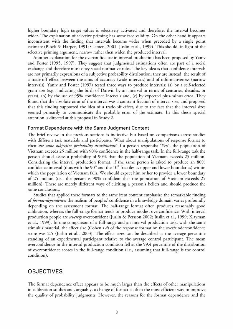
higher boundary high target values is selectively activated and therefore, the interval becomes wider. The explanation of selective priming has some face validity. On the other hand it appears inconsistent with the finding that intervals become wider when preceded by a single point estimate (Block & Harper, 1991; Clemen, 2001; Juslin et al., 1999). This should, in light of the selective priming argument, narrow rather then widen the produced interval.

Another explanation for the overconfidence in interval production has been proposed by Yaniv and Foster (1995, 1997). They suggest that judgmental estimations often are part of a social exchange and therefore must obey social normative rules. The key idea is that confidence intervals are not primarily expressions of a subjective probability distribution; they are instead the result of a trade-off effect between the aims of accuracy (wide intervals) and of informativeness (narrow intervals). Yaniv and Foster (1997) tested three ways to produce intervals: (a) by a self-selected grain size (e.g., indicating the birth of Darwin by an interval in terms of centuries, decades, or years), (b) by the use of 95% confidence intervals and, (c) by expected plus-minus error. They found that the absolute error of the interval was a constant fraction of interval size, and proposed that this finding supported the idea of a trade-off effect, due to the fact that the interval sizes seemed primarily to communicate the probable error of the estimate. In this thesis special attention is directed at this proposal in Study 2.

Format Dependence with the Same Judgment Content The brief review in the previous sections is indicative but based on comparisons across studies with different task materials and participants. What about manipulations of response format to elicit the same subjective probability distribution? If a person responds; “Yes”, the population of Vietnam exceeds 25 million with 90% confidence in the half-range task. In the full-range task the person should assess a probability of 90% that the population of Vietnam exceeds 25 million. Considering the interval production format, if the same person is asked to produce an 80% confidence interval (thus with the 90th and the 10th fractiles as upper and lower boundaries) within which the population of Vietnam falls. We should expect him or her to provide a lower boundary of 25 million (i.e., the person is 90% confident that the population of Vietnam exceeds 25 million). These are merely different ways of eliciting a person’s beliefs and should produce the same conclusions.

Studies that applied these formats to the same item content emphasize the remarkable finding of format-dependence: the realism of peoples’ confidence in a knowledge domain varies profoundly depending on the assessment format. The half-range format often produces reasonably good calibration, whereas the full-range format tends to produce modest overconfidence. With interval production people are severely overconfident (Juslin & Persson 2002; Juslin et al., 1999; Klayman et al., 1999). In one comparison of a full-range and an interval production task, with the same stimulus material, the effect size (Cohen’s d) of the response format on the over/underconfidence score was 2.5 (Juslin et al., 2003). The effect sizes can be described as the average percentile standing of an experimental participant relative to the average control participant. The mean overconfidence in the interval production condition fell at the 99.4 percentile of the distribution of overconfidence scores in the full-range condition (i.e., assuming that full-range is the control condition).

OBJECTIVES The format dependence effect appears to be much larger than the effects of other manipulations in calibration studies and, arguably, a change of format is often the most efficient way to improve the quality of probability judgments. However, the reasons for the format dependence and the

9

extreme overconfidence with interval production are one of the more puzzling and unsolved questions in research on overconfidence and calibration.

The aim of this thesis is to provide a tentative account of the format dependence effect in the form of a Naïve Sampling Model (Juslin et al., 2004) to explain why interval production makes people especially overconfident in their judgments, and to report some empirical data that test this model. The argument in this thesis is that there is a psychological difference between assessing confidence as a probability (half and full-range) and expressing confidence by eliciting fractiles. This difference rests upon the notion that people are fundamentally intuitive statisticians (Peterson & Beach, 1967) when they describe the available information, but are naïve in the sense that they treat sample properties as direct estimators of population properties (Fiedler, 2000; Fiedler & Juslin, in press).

A NAÏVE SAMPLING MODEL OF FORMAT DEPENDENCE

Sampling: Man as a Naïve Intuitive Statistician Proponents of the heuristic-and-bias paradigm argue that biases in human judgment are to be found in the cognitive processes that act upon the received internal or external information (Gilovich et al., 2002, Kahneman et al., 1982). Bias in human judgment can, however, with equal force be explained by biases in the input information that the cognitive processes act upon (Fiedler, 2000; Fiedler & Juslin, in press).The first main assumption behind the notion of a naïve intuitive statistician is that the cognitive process that operates on the available information (samples) is basically consistent with normative principles of logic and reasoning. Extensive collections of data show that people have a remarkable ability to store frequencies in the form of natural and relative frequencies. In turn, in controlled laboratory studies judgments are often accurate expressions of these frequencies (Estes, 1976; Gigerenzer & Murray, 1987; Peterson & Beach, 1967; Zacks & Hasher, 2002).

The next two assumptions are in fact two sides of the same coin, namely naivety. The first type of naivety is with respect to properties of statistical estimators, such as that of being biased or unbiased. It seems that people take for granted that sample properties directly depict population properties. An example of this is that people accurately assess variance in a sample but fail to understand that sample variance needs to be corrected by n/(n-1) to be an unbiased estimate of population variance (Kareev, Arnon, & Horwitz-Zeliger, 2002). Relatedly, they underestimate the probability of rare events since small samples seldom include rare events (Hertwig, Barron, Weber, & Erev, 2004).

The second type of naivety concerns the effect of external biases on the input information that a judge receives from the environment (Fiedler, 2000). People are naïve in the sense that they assume that the samples that they encounter are random and representative of the environment. I will first describe the former kind of naivety in detail.

Biased and Unbiased Estimators The core idea behind the model is that the different response formats involve different estimators. Probability assessment, as required by the half-range and full-range formats, involves estimation of a population proportion. Sample proportion is an unbiased estimator of the population proportion. That is, when sampling from an urn with a proportion p of red balls, the long-run average sample proportion P of red balls is p. When participants are asked to judge the probability that the population of Vietnam lies between 2 and 15 millions (or that the population of Vietnam exceeds 8 million) they may retrieve similar Asian countries with known population figures and

10

assess the proportion that satisfy this event. In contrast, interval production involves estimation of dispersion. The sample dispersion D is a

biased estimator of population dispersion. That is, when sampling from an urn with a dispersion d the average sample dispersion D is lower then d. When asked to produce an 80 % probability interval for the population of Vietnam, the judge may retrieve similar Asian countries and report limits that include 80% of these values.

If people treat their limited input information (i.e., small samples) naively these response formats will, per se, generate different conclusions regarding the outcome bias in these judgments. When people make probability assessments and these are equivalent or similar to sample proportion, they should only show marginal overconfidence (Juslin et al., 1997; Soll, 1996). On the contrary, when producing confidence intervals – equivivalent to a dispersion –and the judge fails to correct for this bias (e.g., Kareev et al., 2002) the produced intervals are bound to be too tight, leading to overconfidence. Given these estimators, in particular dispersion, the sample sizes which the estimator derives from have consequences. When sample dispersion is based on a very large sample it reflects the population dispersion to a greater extent than when based on a smaller sample.

The cognitive processes are essentially the same with both assessment formats: A sample of similar observations is retrieved from memory and directly expressed as required by the format, as a probability (proportion) for interval evaluation and as dispersion for interval production. There is no bias in the processing of the sample, only naivety in the sense that the sample properties are taken as unbiased estimators of population properties.

Biased and Unbiased Subjective Environmental Distributions A second factor contributing to overconfidence in interval production is that the sample itself may be biased and unrepresentative of the population from which it is derived. This fact could by itself explain many other distortions in people’s judgments (Fiedler, 2000). For example, let the population of all Asian countries define an objective environmental distribution (OED). If a person knows the population figures of, say, six of these countries we can define this knowledge as a subjective environmental distribution (SED). In principle, a person’s SED could be a true random sample of the OED, but more often there is a systematic mismatch between the SEDs and the OEDs. Consider the following example: because of some lately intense media coverage regarding severe overpopulation in Asian countries, large country populations become over-represented in a person’s knowledge of population figures for Asian countries. Suppose further that this fictitious person is asked to produce a confidence interval in which he or she is 90% certain that the population of Vietnam falls. Because of the biased negatively skewed SED of Asian countries, the person defines an interval whose limits are in the extreme upper end of the OED of Asian countries (which in fact is positively skewed). This bias in the SED, the input sample, in general contributes to overconfidence with interval production.

An equation can be derived which defines two major psychological contributions to overconfidence (Juslin et al., 2004):

)()( SEDounoOU += (1)

where OU is the observed over-/underconfidence score, o(n) is the overconfidence added by the naïve interpretation of sample dispersion, and ou(SED) is the over-or underconfidence added by systematic deviations between SEDs and OEDs. Note that for very large or infinite n, o(n) approximates zero.

11

Implementation of the NSM The main processing steps implied by the NSM for the production of confidence intervals and the assessment of probabilities are illustrated below:

1. Retrieval of cues. One or several cues (or facts) relevant to estimate the target quantity are retrieved from long term memory. You may retrieve that Vietnam lies in Asia. The cue(s), in turn, define a corresponding objective environmental distribution (OED) of similar observations in the person’s natural environment (Brunswik, 1955). In this case for the cue “located in Asia” there is an OED defined by the distribution of population figures in Asian countries.

2. Sampling the target values of similar objects. In long term memory a subset of the target values in the OED is stored and these observations define the SED. The target values of a sample of n observations from the SED are retrieved to produce a sample distribution (SD). In this example the person may retrieve the populations of n Asian countries (other than Vietnam) which provide a sample of population figures for countries similar to Vietnam (i.e., in this example the similarity refers to the property of being an Asian country).

3. Naïve estimation. The properties of the SDs are directly taken as estimates of the corresponding properties of the population distributions (i.e., the OEDs):

a. Probability judgment: Given a target event, the subjective probability judgment for the event is the proportion of observations in the SD that satisfy the event. If, for example, the estimate concerns the population of Vietnam and the event is having a population larger than 25 million, the person may retrieve a sample of n known population figures of Asian countries. If m out of these n observations have a population larger than 25 million the probability judgment is m/n.

b. Interval production: The sample dispersion is used to estimate the population dispersion. The fractiles2 of the SD is used as estimates of the fractiles of the OED and the median3 of the SD is used as the point estimate of the target quantity. In our example, to produce a .5 probability interval for the population of Vietnam a person may retrieve a sample of Asian countries and report the first and the third quartile (the 25th and 75th fractiles) within the sample as the interval.

For infinite sample size the processes for interval evaluation (Steps 1, 2, 3a) and interval production (Steps 1, 2, 3b) produce identical results: at small sample sizes they do not!

This is shown in figure 1A which provides a schematic illustration of an OED. Following the example, this would correspond to the OED for populations of Asian countries, for illustrative purpose consider it normally distributed. The xxth fractile of the OED is the target value such that xx% of the OED is equal to or lower than that target value. The limits of the interval in Figure 1A are the 25th and the 75th fractiles of the OED, thus defining an interval around the median within which 50% of the OED falls. That is, 50% of the Asian countries have a population between xx and yy million, where xx and yy defines the actual population values defined by the 25th and 75th fractils correspondingly. With interval evaluation with probability assessment the person is given interval limits and is asked to assess the probability that the target quantity falls within the interval. With interval production the person is given a probability and is asked to produce the limits of a central confidence interval around their best guess for the quantity. 2 There exist several methods for interpolation fractiles from finite samples. The simulation relied on a standard procedure, commonly referred to as the EXCEL method. 3 This interpretation of the point estimate is not crucial to the NSM, it is supported by the observation that even when people assess the means of distributions, their judgments are strongly biased towards the median (Peterson & Miller, 1964).

12

SD, Large Sample

Standardized OED variance

Prob

abili

ty d

ensi

ty

0.000.150.300.450.60

-3.50 -1.75 0.00 1.75 3.50

50%

SD, Small Sample and Centered Interval


Prob

abili

ty d

ensi

ty

0.000.150.300.450.60

-3.50 -1.75 0.00 1.75 3.50

39%

SD, Small Sample and Dislocated Interval


Prob

abili

ty d

ensi

ty

0.000.150.300.450.60

-3.50 -1.75 0.00 1.75 3.50

34%

A

B

C

Figure 1. Panel A: Probability density function for an SD with large sample size The values on the target dimension have been standardized to have mean 0 and standard deviation 1. The interval between the .75th and the .25th fractiles of the SD include 50% of the population values in the OED. Panel B: An SD with sample size 4 with the sample mean at the same place as the mean in the OED. The values on the target dimension are expressed in units standardized against the OED variance. The interval between the .75th and the .25th fractiles of the SD include 39% of the population values. Panel C: Probability density function for a sample of 4 exemplars with the sample mean displaced relative to the population mean. The values on the target dimension are expressed in units standardized against the OED variance. The interval between the .75th and the .25th fractiles of the sample distribution includes 34% of the population values (i.e., on average). The person forms his or her uncertain belief about the target quantity by retrieving a SD of similar observations from the SEDs based on sample size n4. The NSM implies that with interval evaluation there is essentially one factor that contributes to the error rate – to the probability that the quantity falls outside of the interval – and this contributor to the error rate is explicitly represented in the sample: a) Sampling error. To the extent that the pre-defined interval does not include the entire OED, some observations in the SD are likely to fall within and some outside the interval as a consequence of sampling error when observations are sampled from the SED. Knowing that the target quantity belongs to a specific OED therefore implies that the target quantity falls in the interval with a probability p. For example, knowing that a country is Asian implies that its population is between xx and yy million with probability .5. For sampling with replacement sample proportion P is an unbiased estimate of population proportion p (the expected value of P is p). As such, relying on the sample proportion to estimate the population proportion yields accurate judgment.

With, for example, a 50% confidence interval it is expected that 50% of the true values will

4 In this illustration a simplifying assumption about the knowledge state of the person is made: the SED, the target

values from the OED that are known to the person, comprise a perfectly random and representative sub-sample of the OED.

13

fall inside the interval. In regard to interval production with the NSM, there are three contributors to the probability that the target quantity falls outside of the produced interval (the error rate), only one of which is explicitly manifested in the SD:

a) Sampling error: Same as above, for all but the highest confidence levels some target quantities will fall outside the interval. This source of variability or error is explicit in the SD. With correctly estimated fractiles (e.g., random sampling and large n) the target quantity falls outside the interval with probability 1-.xx for an .xx probability interval. This is illustrated in Figure 1A, where the proportion of values falling inside the interval is .5 and the error rate is .5.

b) Error from underestimation of the population dispersion: As discussed above the dispersion of a sample systematically under-estimates the dispersion of the population. This is why, for example, sample variance need to be corrected by 1/ (n-1) to become an unbiased estimator of population variance. Even though the central tendency of the SD coincides with central tendency of OED, for this reason alone, assuming a normal distribution, perfect random sampling, and a sample size of 4, the .5 sample central interval from a SD will include at most 39% of the OED (i.e., the error rate is .61 rather than .5; see Figure 1B).

c) Error from misjudged location of the population distribution: In addition to the above errors, at small sample sizes, the produced interval itself is likely to be randomly dislocated relative to the population distribution (i.e., to an extent measured by the standard error of measurement for the sample mean).Taken this sampling error into account, the sample interval only includes 34% of the true values (error rate 66 %: Figure 1C). The NSM implies that because only the first source of variability (i.e., a above) is explicit in the sample, only the first contributor to the error-rate is taken into account when the intervals are produced. At small sample sizes this produces extreme overconfidence and format dependence.

Predictions To generate predictions, execution of the processing steps (i.e., 1, 2, 3A and 3B above) were implemented in a Monte Carlo simulation. To simulate a general knowledge target variable a database of 188 countries and their population figure listed by the United Nations 2002 were used. The continent functioned as cue (see Juslin et al., 2004, for further details on these simulations)

The predictions are plotted in Figure 2A, based on the assumption that the SED is representative of the OED. As can be seen, the extreme overconfidence bias reported for interval production is reproduced. For example, with sample size 3 only half of the target values are included in the 100% intervals. There is, as expected, an effect of sample size in that smaller samples lead to more overconfidence and the interval size increases with the probability level (i.e., .5, .75 and 1.0). The reason for the overconfidence in Figure 2A is that the NSM only considers the sampling variability that is explicit in the sample, thus ignoring error from underestimation of population dispersion and misplaced intervals.

Now, let a pre-stated interval define the event and the task is to assess the probability that a target variable falls within that interval. This procedure defines the interval evaluation format and is, as discussed, merely another way to express the same uncertain belief about a quantity.

14

Pre-stated subjective probability

Prop

ortio

n co

rrec

t

0.00.10.20.30.40.50.60.70.80.91.0

50 75 100

n=3

n=5n=7

Respons Format

Ove

r/Und

erco

nfid

ence

-0.1

0.0

0.1

0.2

0.3

0.4

0.5

0.6

Production Evaluation

n=7

n=3

n=5

Resampling probability

Form

at D

epen

denc

e

0.0

0.1

0.2

0.3

0.4

0.5

0 .1 .2 .3 .4 .5 .6 .7 .8 .9 1

n=3 n=5 n=7

A B

C

Subjective probability

Prop

ortio

n in

clud

ed

0.0

0.1

0.2

0.3

0.4

0.5

0.6

0.7

0.8

0.9

1.0

50 75 100

Random sampling

U-shaped SED

Negatively skewed SED

D

Figure 2. Predictions by the NSM. Panel A: Proportion of correct target values included in the intervals for the three different probabilities with different sample size (n). The dotted line is the proportions required for perfect calibration. Panel B: The format dependence (i.e., difference between overconfidence with interval production and interval evaluation) predicted for independent samples. Panel C: The predicted format dependence as a function of the resampling probability when the two samples are not independent. Panel D: Interval production simulated with random sampling and sampling from different biased SEDs (u-shaped and negatively skewed) applied on a positively skewed OED. This format is, if the NSM is correct, psychologically different and should generate different conclusions about overconfidence when compared to interval production. To simulate the interval evaluation format the produced intervals in Figure 2A defined the events and the model was fed with a new independent random sample of items. NSM was then asked, so to speak, to assess the probability that the target value falls within the pre-stated interval according to processing steps 1, 2 and 3A above. With interval evaluation the probability judgments were nearly the same as the corresponding proportion correct with interval production in Figure 2A and overconfidence thus close to zero. Figure 2B illustrates the difference between the two formats, where the over/underconfidence score is the mean probability attached to interval minus the proportion of values that falls within the interval. With the interval evaluation format the overconfidence is eliminated. The explanation for this effect is that interval evaluation is not a biased estimator and errors from too small and displaced interval become explicit in the sample.

In regard to the degree of format dependence an important distinction is whether the event (e.g., a pre-stated interval) is statistically independent or dependent of the sample used to make the probability judgment. An event can be considered as independent if it is defined a priori without knowledge of possible samples that judges may use to estimate the probability of that event. For example, this is appropriated when the assessment concerns future events such as meteorology forecasts (Murphy & Winkler, 1977) or when general knowledge items are randomly selected from natural environments (Gigerenzer et al., 1991; Juslin, 1994; Juslin et al., 2000). The opposite case is when there is a statistical dependence between sample and event. For

15

example, consider an extreme case were exactly the same SED is used to produce and evaluate the same interval (e.g., the same person makes this judgment for the same uncertain value). If this is the case no format dependence will exist. This can also be the case between persons, if people only know a small sample of the environment and this knowledge overlaps to a high extent because of media coverage (Fiedler, 2000).

In the simulation this dependence is interpreted as a resampling probability between 0 and 1; that is, the probability that an item used first to produce an interval is re-sampled and used for interval evaluation. Figure 2C shows how this affects the format dependence: as when the resampling probability increases the format dependence is predicted to shrink.

The consequences that the biased SEDs have for the overconfidence in interval production, modeled according to NSM, are shown in Figure 2D. The NSM was modeled with an idealized positively skewed beta OED distribution where intervals were created from a negatively skewed and a u-shaped beta SED distribution. As can be seen in Figure 2D a u-shaped SED will almost completely wipe out the overconfidence found under the random sampling assumption and a negatively skewed SED will lead to even more severe overconfidence than found under the random the sampling assumption.

In sum, the NSM predicts a substantial format dependence effect between interval production and interval evaluation when judgments are based on small samples. The format dependence is predicted to decrease as a function of the degree of statistical dependence between the sample and the event.

Constraints on Sample Size As we saw in the predictions (Figure 2A) overconfidence in interval production and format dependence is a function of sample size. This might suggest that with more knowledge (e.g., expert judges) we should expect a decrease in overconfidence and format dependence. However, limited computational capacity is an important result in cognitive psychology, characterized by Miller’s (1956) “seven-plus-or-minus-two” estimate of our short term memory capacity. The role of a constrained working memory capacity have gained support in numerous domains (Baddeley, 1998), including problem solving (Newell & Simon, 1972) reasoning (Evans, 2002) and reading comprehension (Just & Carpenter, 1992). In contrast, in judgment research capacity constraints have served as a rationale for the influential research program on judgmental heuristics (Gilovich et al., 2002; Kahneman, et al., 1982), but detailed explorations on the role of working memory are more rare. This fact raises interesting research questions along with the NSM regarding possible constraints on the samples that are retrieved from memory. Is the retrieved sample constrained by working memory limitations? This suggest that, despite the total sample of stored knowledge in long-term memory, when faced with these kinds of judgments only a sample with a size determined by working memory can be used. If this is the case overconfidence and format dependence should be equally large independently of the total sample that has been experienced by the judge. An alternative interpretation is that the process draws on knowledge crystallized over long time summarizing the complete sample, or most, of the observations experienced. The latter possibility suggests that overconfidence and format dependence should decrease in expert judges with larger samples.

EMPIRICAL STUDIES The two empirical studies included in this thesis should be regarded as tests of the underpinning

16

of the NSM with both general knowledge items and in controlled learning experiments. Study 1 investigates if it is possible to reduce or even cure the overconfidence bias using interval evaluation and if the degree of format dependence varies when manipulating the dependence between the sample and the event. Study 2, with a controlled experimental learning setting, investigates in more detail possible sampling constraints and biased SEDs by applying Eq. 1 to overconfidence in interval production.

Study 1 In Study 1 interval production is directly compared with interval evaluation (e.g., What is the probability that the population of Vietnam lies between 15 and 25 million?) which involves assessment of two fractiles of the subjective probability distribution. Previous studies have compared interval production with assessment formats that only involves one fractile of the distribution (e.g., What is the probability that the population of Vietnam exceeds 25 million?) This first study consists of two experiments that involve general knowledge items. The task was to produce and evaluate intervals about the population figures in different world countries defined by United Nations database (2002).

Experiment 1 The interval evaluation format has not been previously examined; the purpose was to corroborate the predicted format dependence for interval production and interval evaluation. To investigate format dependence, both between and within–subjects designs were used which allow a test of the effect of the dependence between the sample and the event.

Forty undergraduate students from Umeå University participated in the experiment. One group of 20 participants (the P-group) produced 50, 75 and 100% intervals (at the first occasion, t1). One week later (occasion t2a) the participants in the P-group returned and made interval evaluations where the event was defined by the intervals produced at t1. The task was ended with additional interval productions (t2b). The second group of 20 participants (the E-group) made interval evaluations where the events were defined by the intervals produced by the P-group at t1. The E-group ended the task by producing intervals.

The rationale for using this design was that it provided the possibility to compare over- or underconfidence with interval production and interval evaluation applied to the same intervals (events) but carried out by different judges. The prediction was as follows: a) format dependence was expected between interval production and interval evaluation in general, b) the largest effect was expected between subjects (P-Group vs. E-group), c) the smallest amount of format dependence was expected within the P-Group and, d) format dependence of a similar magnitude as in prediction b was expected within the E-Group. The reason for prediction c is that when participants evaluate the same interval as they have produced by themselves the statistical dependence between the sample and the event should be high (i.e., a high resampling probability). The reason for prediction d was that, although a within-subjects comparison, the evenst (the intervals) were defined by other participants (i.e., the P-Group) and the statistical dependence between the sample and the event should be low (i.e., low resampling probability).

Results As predicted, the format dependence effect is observed when comparing interval production and interval evaluation. When the data was collapsed across all interval productions and interval evaluations there is significantly more overconfidence with interval production, see Figure 3A. In Figure 3B, which shows the between subjects comparison, the format dependence effect is more

17

profound than in Figure 3C. The reason for this is that the samples used to produce and evaluate intervals in Figure 3C overlap to a greater extent than in Figure 3B.

Total Format Dependence

Format

Ove

r/und

erco

nfid

ence

0.0

0.1

0.2

0.3

0.4

0.5


Between-Subjects

Format

Ove

r/und

erco

nfid

ence

0.0

0.1

0.2

0.3

0.4

0.5


Within-Subjects, Own Intervals

Format

Ove

r/und

erco

nfid

ence

0.0

0.1

0.2

0.3

0.4

0.5

Prod. (t1) Eval. (t2a) Prod. (t2b)

Within-Subjects, Other's Interval

Format

Ove

r/und

erco

nfid

ence

0.0

0.1

0.2

0.3

0.4

0.5

Prod. (t2b) Eval. (t2a)

A B

C D

Figure 3. Experiment 1: Panel A: Main effect of interval production and interval evaluation on the overconfidence score (95% CI, n=20). Panel B: Between-subject comparison of overconfidence for interval production and interval evaluation, low sample overlap predicted (95% CI, n=20). Panel C: Within-subject comparison of the P-groups’ overconfidence for interval production and interval evaluation, high sample overlap predicted (95% CI, n=20). Panel D: Within-subject comparison of the E-groups overconfidence for interval production and interval evaluation, low sample overlap predicted (95% CI., n=20). The Figure is reproduced from Winman, A., Hansson, P., & Juslin, P. (2004). Subjective Probability Intervals: How to Reduce Overconfidence by Interval Evaluation. Journal of Experimental Psychology: Learning, Memory, and Cognition, 30, 1167-1175. In Figure 3D the magnitude of the effect is comparable with that in Figure 3B, despite the fact that this comparison is made within subjects. In this case the intervals which define the events are produced by another person; there is less dependence between the samples and the events. Figure 3C shows the robustness of the effect, the participants in the P-Group reverted to being significantly more overconfident when they produced intervals at the second occasion.

Experiment 2 This experiment relied on an adaptive interval adjustment (ADINA) procedure that changes the interval production task into a task more similar to interval evaluation. The core idea behind ADINA is that the end product still is an interval, but the procedure requires assessment of probability rather than dispersion. Here the participants were presented with pre-stated intervals which change in size in response to the previous evaluation with the effect that the intervals home in on the target probabilities .5, .8, and 1.0. The prediction was that this apparently inconsequential procedure change should reduce overconfidence. The ADINA has potential as a debiasing tool in an applied approach, if effective. This procedure also addresses some objections that could be raised against the interpretation of Experiment 1, such as memory and regression effects and, deviations between the response variables (probability vs. intervals). In Experiment 2

18

no repeated measures were used and all participants produced intervals. Forty-five undergraduate students from Umeå University participated in the experiment.

Three between-subjects conditions were used. A control-condition with interval production, an ADINA(O) condition in which the first interval was centered on the participant’s own point estimate, and an ADINA(R) condition in which the first interval was centered on a random value.

With this design it was possible to control the dependence between sample and event. The ADINA(O) condition should lead to high dependency because the interval (which was centered around the point estimate) was presumably affected by the same sample that was used for the interval evaluation. However, in the ADINA(R) condition the former dependence does not hold due to the randomly centered intervals, thus formed independently of the participant’s knowledge (sample). This independence strictly holds only for the first interval, already with the second judgment the size of the interval is a function of the participant’s knowledge.

Thus, the predictions were: overall, the ADINA procedure should reduce overconfidence because the estimator is a proportion instead of dispersion; the strongest effect should be between the control condition (interval production) and ADINA(R) condition (first intervals).

Results In general the ADINA produced significantly less overconfidence then the control condition.

First Interval

Condition

Pro

babi

lity

0.0

0.1

0.2

0.3

0.4

0.5

0.6

0.7

0.8

0.9

1.0

Control ADINA(O) ADINA(R)

Proportion correctSubjective probability

Final Interval

Condition

Pro

babi

lity

0.0

0.1

0.2

0.3

0.4

0.5

0.6

0.7

0.8

0.9

1.0

Control ADINA(O) ADINA(R)


Calibration Graph

Subjective probability

Pro

porti

on c

orre

ct

0.0

0.1

0.2

0.3

0.4

0.5

0.6

0.7

0.8

0.9

1.0

0 .1 .2 .3 .4 .5 .6 .7 .8 .9 1.0

ControlADINA(R)

A B

C

Figure 4. Panel A: Mean confidence and proportion of intervals that include the population value as computed from the response to the first a priori interval (with 95% CI, n=15). Panel B: Mean confidence and proportion of intervals that include the population value as computed of the final “homed in” probability intervals (with 95% CI, n=15). Panel C: A calibration curve where the proportion correct is plotted against subjective probability based on all the data from the control and the ADINA(R)-conditions. The dotted line represents perfect calibration. Overconfidence is the difference between the mean confidence and the proportion. The Figure is reproduced from Winman, A., Hansson, P., & Juslin, P. (2004). Subjective Probability Intervals: How to Reduce Overconfidence by Interval Evaluation. Journal of Experimental Psychology: Learning, Memory, and Cognition, 30, 1167-1175.

19

Figure 4 shows the overconfidence for the three experimental conditions. As predicted the largest difference in overconfidence is seen between the control condition and the ADINA(R) condition where the decoupling of dependence is best approximated, and there are close to zero overconfidence, see Figure 4A. The same rank order is seen in Figure 4B, final interval, but now with overconfidence in all three conditions. This should be the case if the dependence between knowledge used to produce and evaluate interval is a crucial factor. Figure 4C shows a calibration graph where the within-rang proportion is plotted against the subjective probability. All judgments in the ADINA(R) condition are included. Despite this fact the difference is striking.

Discussion Experiment 1 successfully confirmed the predicted format dependence by the NSM, interval evaluation leads to more realistic judgments compared to interval production. The most striking results are that this effect is seen even in a within-subjects comparison when a participant produce and evaluate the same interval. Participants that first produced intervals, then returned and made interval evaluation, and again produced intervals returned to their initial extreme overconfidence. This, by itself, implies that there are some fundamental divergence between production and evaluation of probability intervals in line with the fundamentally different properties suggested by the NSM.

In Experiment 2 the overconfidence bias is almost completely wiped out, as predicted by the NSM when no dependence exists between the knowledge used to make the assessment and the event which is assessed. The ADINAs superiority, regardless of dependence, suggests that it could be successfully used in an applied setting where it is necessary to define upper and lower limit of some unknown quantity. The results from Experiment 2 also rules out possible alternative interpretations of the results from Experiment 1, such as memory carryover effects, regression effects, and different response variables.

One important issue concerns the fundamental psychological nature of the two response formats. Interval production involves judgment about a person’s own knowledge, a fact that may contribute an affective component which could increase overconfidence (Taylor & Brown, 1988). This interpretation appears inconsistent with the almost zero overconfidence observed in the two alternative-half-range format where the participants first must choose an alternative, which is clearly reflecting the person’s own knowledge (Juslin & Persson, 2002; Juslin et al., 1999). It is also inconsistent with the actor-observer paradigm were observers who rate confidence in another person’s judgment are no less and sometimes more overconfident then the judge himself (Koehler & Harvey, 1997).

Study 2 In Study 2 confidence judgments are investigated in a learning paradigm which has not been used in previous research. The advantage is that this makes it possible to manipulate and control the sample sizes of the participants and the SEDs and thereby get a deeper understanding of the processes that are at work. In two experiments are working memory capacity related to the results on overconfidence and format dependence.

As mentioned above, Yaniv and Foster (1997) proposed an idea that confidence judgment in the form of interval production does not convey a subjective probability distribution but is a trade-off effect. The support for this idea was that the absolute error was a fraction of the interval size. The NSM also predicts this finding with the explanation that the precision of the interval is determined by only two retrieved observations, those that define the interval in the SD, regardless of what confidence is at stake. Both interval size and the accuracy of the midpoint are therefore

20

functions of the variance in the SED. In Figure 5 the absolute error of the midpoints is plotted against interval size when the NSM was applied to the same database as used in the experiments reported below. As can be seen this produces a very characteristic bivariate distribution and relationship between absolute error and interval size. There is a constant positive slope between the absolute error and interval size; there are also two separate clusters of absolute error for the low interval sizes.

Statistical Confidence Intervals

Interval Size

Stan

dard

Err

or

0

400

800

1200

1600

0 400 800 1200 1600

50% CI, n = 4 50% CI, n = 8 75% CI, n = 4 75% CI, n = 8 95% CI, n = 4 95% CI, n = 8

OU = 0

.5 Interval by NSM(n=4)

Interval Size

Abs

olut

e Er

ror

0

400

800

1200

1600

0 400 800 1200 1600

y = 22.8 + 0.48 * x

OU = .15

.75 Interval by NSM(n=4)

Interval Size

Abs

olut

e Er

ror

0

400

800

1200

1600

0 400 800 1200 1600

y = 20.0 + 0.47 * x

OU = .29

1.0 Interval by NSM(n=4)

Interval Size

Abs

olut

e Er

ror

0

400

800

1200

1600

0 400 800 1200 1600

y = 15.0 + 0.46 * x

OU = .40

A B

C D

Figure 5. Panel A: The relationship between the standard error of the midpoint of the interval and the interval size, as a function of the probability of the confidence interval and the sample size, for “real” confidence intervals computed according to statistical theory. Predicted relationship between interval sizes and absolute error, and the overconfidence predicted by the NSM with sample size 4 (NSM (n=4)), separately for .5 (Panel B), .75 (Panel C), and 1.0 (Panel D) confidence intervals. Note also that the slope between the absolute error and interval size almost is identical for the three probability levels. This coincides with the results reported by Yaniv and Foster (1997), but here it is derived from the NSM without assuming any trade-off effects. Figure 5A shows real statistical confidence intervals. With these normative intervals the slope between standard error and interval size decreases with the probability. These are “real” confidence intervals and should produce zero overconfidence. Comparison between these predictions and the empirical data is later performed.

Experiment 1 The first experiment aims to replicate the format dependence between interval production and interval evaluation under controlled learning conditions and extreme uncertainty. The judgment task was to learn quarterly income figures for fictive companies. Forty students from Umeå University, twenty in each group, participated. 136 different companies defined the OED and each participant was randomly exposed, only once, to half (i.e., 68) of these companies with feedback in the training phase. In the test phase, half of the participants produced intervals in the same manner as in Study 1, Experiment 2 (Control) for all of the 136 companies in the OED.

21

The other half made interval evaluations on all of the 136 companies as in Study 1, Experiment 2 (ADINA (R), First Interval). To assess the participants working memory capacity a digit-span test was used. This test encompassed two sub-tests: a passive repeat back test of random numbers between 0 and 9 and a procedure which required the participants to repeat the numbers in ascending order.

Results Approximately 12 out of 136 companies were successfully recalled in the test phase. The format dependence between interval production and interval evaluation is illustrated in Figure 6. As can be seen interval production yields significantly more overconfidence then interval evaluation.

Condition

Pro

babi

lity

0.0

0.1

0.2

0.3

0.4

0.5

0.6

0.7

0.8

0.9

1.0

Interval Production Interval Evaluation


Figure 6. Mean subjective probability and mean proportion of in-range values with 95% statistical confidence intervals across participants in Experiment 1 (n = 20).

Eq. 1 was applied in a linear multiple regression model with overconfidence as the dependent variable and working memory and SED bias as the independent variables. However, overconfidence was not well predicted by either working memory or SED bias. The SED bias is defined by the absolute deviation between the mean objective quarterly income and the mean correctly recalled income. When analyzing the variance of the recalled target values by a median split between those with low and high variance it showed that this was an important predictor for overconfidence. Those participants with low variance were almost twice as overconfident as those with high variance (.38 vs. .17: F(1, 18) = 6.00, p=.025). This finding might suggest that variation among the small sub-samples that each participant happened to encounter surpasses the relatively small variation in working memory capacity.

Experiment 2 This experiment extended the training phase. In this task, all of the participants observed exactly the same information (i.e., they were exposed to all of the companies in the OED) and the manipulation regarded the degree of training received in the training phase. Thirty students from Umeå University participated. One group (i.e., the 2x Training condition) of participants received 2 blocks of training (272 trials), the other group of participants (i.e., the 4x Training condition) received 4 blocks of training (544 trials).

22

The judgment task, the materials and the procedure were the same as in Experiment 1, but the amount of training was manipulated and the test phase only involved production of intervals. For this reason a comparison across experiments (i.e., the interval productions with .5 block of training) was conducted.

If working memory is of importance for the determination of sample size, there should be no effect of training and a substantial negative correlation between working memory capacity and overconfidence. If it is the content stored in long-term memory that constrains the sample size, then training should reduce overconfidence and no significant correlation should be expected between working memory capacity and overconfidence.

Results Figure 7 summarize the results from the two groups in Experiment 2 and the interval production

Recalled Target Values

Training Blocks

Prop

ortio

n R

ecal

led

0.0

0.1

0.2

0.3

0.4

0.5

0 1 2 3 4

F2,47 = 9.17, MSE = .026, p = .000

Overconfidence for Estimates

Training Blocks

Ove

rcon

fiden

ce

0.0

0.1

0.2

0.3

0.4

0.5

0 1 2 3 4

F2,47 = .80, MSE = .031, p = .45

NSM(n=4)

A

B

Figure 7. Panel A: Proportion of correctly recalled exact target values in the condition with half a block of training (Experiment 1), and with 2 and 4 blocks of training (Experiment 2). Panel B: Overconfidence across intervals where the exact correct target value was not recalled in the condition with half a block of training (Experiment 1), and with 2 and 4 blocks of training (Experiment 2), along with the overconfidence predicted by NSM (n=4).

group in Experiment 1. Panel A shows that the proportion of recall responses increases significantly with training. Panel B shows that the degree of learning or training has little effect on the overconfidence, as indicated by the non significant difference between the three groups.

Table 1 presents the results of applying Eq. 1 in a linear multiple regression model with overconfidence as the dependent variable and working memory and SED bias as the independent variables for the two conditions. This time the regression model shows good prediction of the participant’s overconfidence, with significant contributions both by working memory and SED bias (2 blocks of training). With four training blocks the regression model allowed even better

23

prediction, but now the dominant contribution was working memory capacities alone, which suggest that all of those participants had attained fairly accurate SEDs. Table 1 Linear Multiple Regression Models with Over-/underconfidence as Dependent Variable (regressor), and Working Memory Capacity and SED Bias as the Independent Variables (predictors). Half a Block of Training Refers to Experiment 1; 2 and 4 Blocks of Training to Experiment 2

Model Working Memory SED Bias Blocks of training R N p β t p β t p

.5 Blocks .12 20 .89 -.11 .43 .67 .03 .12 .90 2 Blocks .77* 15 .005 -.70* 3.72 .003 .47* 2.48 .029 4 Blocks .80* 15 .002 -.80* 4.57 .001 -.05 .29 .80

Note: R = Multiple correlation; N = Number of independent observations; p = p-value associated with model or β

weight; β = Beta weight for the predictor; t = t-statistic. * Correlations statistically significant beyond alpha .05.

Figure 8 plots the mean absolute error for each of the assessed companies against the corresponding mean interval size. As predicted by the NSM (compare with Figure 5B, C, and D), size and mean overconfidence increases with the probability attached to the intervals.

.5 Interval

Interval Size

Mea

n A

bsol

ute

Erro

r (M

AE)

0

400

800

1200

1600

0 400 800 1200 1600

y = 27.5 + 0.54*x

OU = .10

.8 Interval

Interval Size

Mea

n A

bsol

ute

Erro

r (M

AE)

0

400

800

1200

1600

0 400 800 1200 1600

y = 26.7 + 0.52*x

OU = .32

1.0 Interval

Interval Size

Mea

n A

bsol

ute

Erro

r (M

AE)

0

400

800

1200

1600

0 400 800 1200 1600

y = 21.4 + 0.46*x

OU = .40

A

B

C

1/2 Block of Training

.5 Interval

Interval size

Mea

n A

bsol

ute

Erro

r (M

AE)

0

400

800

1200

1600

0 400 800 1200 1600

y = 16.8 + 0.49*x

OU = .11

.8 Interval

Interval Size

Mea

n A

bsol

ute

Erro

r (M

AE)

0

400

800

1200

1600

0 400 800 1200 1600

y = 22.4 + 0.45*x

OU = .30

1.0 Interval

Interval Size

Mea

n A

bsol

ute

Erro

r (M

AE)

0

400

800

1200

1600

0 400 800 1200 1600

y = 4.1 + 0.46*x

OU = .33

.5 Interval

Interval Size

Mea

n A

bsol

ute

Erro

r (M

AE)

0

400

800

1200

1600

0 400 800 1200 1600

y = 27.1 + 0.40*x

OU = .10

.8 Interval

Interval Size

Mea

n A

bsol

ute

Erro

r (M

AE)

0

400

800

1200

1600

0 400 800 1200 1600

y = 28.9 + 0.47*x

OU = .25

1.0 Interval

Interval Size

Mea

n A

bsol

ute

Erro

r (M

AE)

0

400

800

1200

1600

0 400 800 1200 1600

y = 8.3 + 0.48*x

OU = .30

2 Blocks of Training 4 Blocks of Training

Figure 8.: Observed relationship between interval sizes and absolute error and the observed overconfidence bias in the condition with half block of training in Experiment 1(Left), two blocks of training in Experiment 2 (Middle), and four blocks of training Experiment 2 (Right), separately for .5 (Panel A), .75 (Panel B), and 1.0 (Panel C) probability intervals.

Note also that the regression line is the same for all three probability intervals, .5, .8 and 1.0, and that the same bivariate distribution is observed with similar signs of two distinct clusters of mean

24

absolute error for small interval sizes as predicted by the NSM (see Figure 5). There is an astonishing resemblance between the prediction by the NSM in Figure 5 and the observed data in Figure 8.

Discussion The format dependence effect was reproduced under conditions of extreme uncertainty (see Figure 6). Note that this comparison is based on exactly the same stimuli and amount of training. This finding, if anything, supports the idea of the superiority of interval evaluation in applied settings. The absence of a correlation between working memory and overconfidence in Experiment 1 could be explained by the very small and highly variable individual SEDs encountered during the minimal training. This idea is supported by the comparison of the overconfidence for participants with high and low subjective variance in the estimates. The goal of Experiment 1, to replicate the format dependence with the learning paradigm, was successfully achieved but we failed to confirm the predicted correlation between working memory and overconfidence.

The finding that learning had no impact on overconfidence in interval production (see Figure 7A and B) is a remarkable finding. What is even more interesting is the strong negative correlation between working memory and overconfidence which supports the idea that working memory is a constraining variable that should be considered also in judgment and decision research. These results clearly illustrate that more experience not necessarily, in isolation. reduces overconfidence, a finding that is in line with previous studies on expert judges outside of the laboratory (Russo & Schoemaker, 1992). Note also that these results were obtained in an environment with instantaneous and error-free feedback. Lack of accurate feedback has sometimes been proposed as one reason for overconfidence in expert judges. (e.g., Russo & Schoemaker, 1992).

CONCLUSIONS AND GENERAL DISCUSSION This thesis tackles the astonishing finding of format dependence in subjective probability calibration. That is, when people express their belief about some unknown quantity as a probability interval they show severe overconfidence, a finding that is almost completely abolished when the same belief is expressed in the form of a probability assessment for a pre-stated interval. A tentative explanation was given for this effect in the form of a Naïve Sampling Model (Juslin et al., 2004) which states that the human mind can be likened to a naïve intuitive statistician with cognitive processes that accurately describes the available sample of knowledge, but is naïve with respect to properties of statistical estimators and biased input samples (Fiedler, 2000; Fiedler & Juslin, in press). The NSM predicted that it should be less overconfidence bias with interval evaluation as compared to interval production on the assumption that these two assessment formats invoke two psychologically different estimators: proportion (interval evaluation) and dispersion (interval production), where the former is an unbiased estimator of population proportion and the latter is a biased estimator of the population dispersion. The degree of this format dependence effect is a function of the statistical dependence between the sample and the event.

In Study 1, Experiment 1 this prediction was successfully verified both from the point of view of within and between-subjects comparison (see Figure 3). The between-subjects and between event comparison showed the largest format dependence and this effect was reduced when the same participants evaluated their own intervals. Experiment 2, Study 1, shows that it is almost possible to eliminate the overconfidence bias with interval evaluation (see Figure 4). A special

25

procedure for elicitation of subjective probability, ADINA, was successfully applied which could be used as a debasing tool in applied settings.

In Study 2, a controlled learning experiment, the format dependence between interval production and interval evaluation was replicated under conditions of extreme uncertainty. More interesting, the amount of learning had no effect on the degree of overconfidence in interval production. The hypothesis that sample size is constrained by working memory capacity was supported by the significant negative correlations between working memory and overconfidence (see Table 1). This result should, of course, be interpreted with care since no correlation was found in Experiment 1, Study 2, even if the variation among the small sub-samples that each participant happened to encounter could exceed the small variation in working memory capacity. However, the results from Study 2 makes a moderate suggestion that limited computational capacity by working memory, at least, should be considered in subjective probability calibration research. In all three interval production conditions in Study 2 the absolute error of the midpoint of the intervals was a constant fraction of the interval size (see Figure 8), a result that verifies the predicted pattern made by the NSM. This finding, and the fact that both interval size and the in-range proportion increases with probability suggests that when people make these kinds of judgments they primarily express a subjective probability distribution. Nonetheless, no results in this thesis directly rule out the possibility that people are engaged in a trade-off between accuracy and infomrmativeness. On the other hand, that the NSM predicts the same pattern is at least a complication for the trade-off explanation proposed by Yaniv and Foster (1997).

What about priming effects that seem to reduce overconfidence in interval production (Block & Harper, 1991, Clemen, 1992; Juslin et al., 1999; Soll & Klayman, 2004) and the NSM? One suggestion is that the observations that are retrieved from long-term memory, when asked for an initial point estimate, may stay active in working memory. This would imply that the actual sample size, when producing the interval immediately after a point estimate, exceeds that of only producing an interval without any priming of additional estimate. This notion is exemplified by the NSM in Figure 2A. When a sample of 3 items is extended with additionally 2 items the hit-rate for a 75% interval increases with 12 percentage units.

What is the appropriate interpretation of the NSM? In the way the NSM has been presented in this thesis, that people have a stored collection of similar observations that are retrieved and expressed in the judgments, suggests that the NSM is a model on the algorithm level. The limitation of this interpretation is that to become a full feathered algorithm model that is psychologically plausible the NSM needs, for example, assumptions about how similarity affects judgments (Dougherty, Gettys, & Ogden, 1999; Juslin & Persson, 2002; Sieck & Yates, 2001). The NSM could, however, be amended with PROBEX (Juslin & Persson, 2002) which is an exemplar algorithm of similarity-graded probability. When the retrieval process of a sample from memory has been provided by PROBEX, people act upon these retrieved exemplars as outlined by the NSM. On the other hand the NSM could be interpreted as a computational level theory (Marr, 1982) that specifies what function is computed by the mind, regardless of the underling cognitive processes, representations etc. In this sense the NSM states that the function computed by the mind is that of a naïve intuitive statistician.

From the heuristic-and-biases point of view one could argue that the naiveté of using a biased estimator such as dispersion and not appreciating the need to correct the estimates is a typical cognitive processing deficiency which should be sorted under the representativeness heuristics. It is true that the NSM suggests similar claims as “the law of small numbers” in which people regard small samples to be highly representative of the population (Tversky & Kahnemn, 1971; Tversky & Kahneman, 1974). According to the NSM, however, people do not compute a biased representation of the input sample. Instead, the computation is appropriate for large samples. And if considering the fact that the sample size could be constrained by working memory capacity, would we then regard such a hardwired constraint a cognitive processing bias? In any case, the

26

NSM acts as a more detailed cognitive theory and provides variables of importance to understand the underlying processes that generates overconfidence with interval production and how to cure it.

What about gender differences? Soll and Klayman (2004) did find gender differences with interval production regarding overconfidence; men were more overconfident than women. If women should be less overconfident than men it does not make any menace to the robust reduction of overconfidence with interval evaluation.

The assumption that people use the dispersion within the sample to estimate the population dispersion without corrections could, of course, be more specified. Do people respond to the rank order of the observations in the sample or do they compute something like the variance, and fail to correct it by n/(n-1)? This question requires further investigations. Another interesting challenge for the NSM is to capture the strong format dependence effect that has also been observed in sensory discrimination tasks (e.g., Juslin et al., 2003). Could the NSM be generalized to explain phenomena in, for example, visual perception? This evokes inspiring further research. The effect of working memory capacity on overconfidence needs to be corroborated in additional experiments; it could also be combined with other cognitive measures, such as episodic memory and IQ. The assumption that SED bias in some circumstances could reduce overconfidence in interval production (see Figure 2D) needs empirical support. One possible means to test this assumption would be to conduct a learning experiment in which the shape of SED is manipulated between participants.

This thesis ends with a recommendation: if you want to receive realistic judgments concerning some continuous quantity (e.g., interest-rate, stock value etc.), provide an interval, and do not let the judges define it!

27

REFERENCES Alba, J., W., & Hutchinson, W., J. (2000). Knowledge calibration: What consumers know and

what they think they know. Journal of Consumers Research, 27, 123-156. Alpert, W., & Raiffa, H. A. (1982). A progress report on the training of probability assessors. In

D. Kahneman, P. Slovic & A. Tversky (Eds.), Judgments under uncertainty: Heuristics and Biases. (pp. 294-305). New York: Cambridge University Press.

Allwood, C., M., & Montgomery, H. (1987). Response selection strategies and realism of confidence judgments. Organizational Behavior and Human Decision Processes, 39, 365-383.

Allwood, C., M., & Granhag, A., G. (1996a). Considering the knowledge you have: Effects on realism in confidence judgments. European Journal of Cognitive Psychology, 8, 235-256.

Allwood, C., M., & Granhag, A., G. (1996b). Realism in confidence judgments as a function of working in dyads or alone. Organizational Behavior and Human Decision Processes, 66, 277-289.

Baddeley, A. (1998). Recent developments in working memory. Current Opinion In Neurobiology, 8, 234-238

Björkman, M. (1994). Internal cue theory: Calibration and resolution of confidence in general knowledge. Organizational Behavior and Human Decision Processes, 57, 386-405.

Block, R., & Harper, D. (1991). Overconfidence in estimation: Testing the anchoring-and-adjustment hypothesis. Organizational Behavior and Human Decision Processes, 49, 188-207.

Brenner, L. (2000). Should observed overconfidence be dismissed as a statistical artifact? Critique of Erev, Wallsten, & Budescu (1994). Psychological Review, 107, 943-946.

Brenner, L. (2003). A random support model of the calibration of subjective probabilities. Organizational Behavior and Human Decision Processes, 90, 87-110.

Brenner, L., Koehler, D., Liberman, V., & Tversky, A. (1996). Overconfidence in probability and frequency judgments: A critical examination. Organizational Behavior and Human Decision Processes, 65, 212-219.

Brunswik, E. (1955). Representative design and probabilistic theory in a functional psychology. Psychological Review, 62, 193-217.

Clemen, R. T. (2001). Assessing 10-50-90s: A surprise. Decision Analysis Newsletter, 20, 2, 15. Dhami, M., Hertwig, R., & Hoffrage, U. (2004). The role of representative design in an

ecological approach to cognition. Psychological Bulletin, 130, 959-988. Dougherty, M. R. P., Gettys, C. F., & Ogden, E. E. (1999). MINERVA-DM: A memory

processes model for judgments of likelihood. Psychological Review, 106, 180-209. Erev, I., Wallsten, T. S., & Budescu, D. V. (1994). Simultaneous over- and underconfidence:

The role of error in judgment processes. Psychological Review, 101, 519-527. Estes, W. K. (1976). The cognitive side of probability learning. Psychological Review, 83, 37-64. Evans, J. S. (2002). Logic and human reasoning: An assessment of the deduction paradigm.

Psychological Bulletin, 128, 978-996. Fiedler, K. (2000). Beware of samples! A cognitive-ecological sampling approach to judgment

biases. Psychological Review, 107, 659-676. Fiedler, K., & Juslin, P. (in press). Taking the interface between mind and environment seriously.

In K. Fiedler, & P. Juslin (Eds.), Information sampling as a key to understand adaptive cognition. New York: Cambridge University Press.

Gigerenzer, G., & Murray, D. J. (1987). Cognition as intuitive statistics. Hillsdale, NJ: Lawrence Erlbaum Associates.

28

Gigerenzer, G., Hoffrage, U., & Kleinbölting, H. (1991). Probabilistic mental models: A Brunswikian theory of confidence. Psychological Review, 98, 506-528.

Gilovich, T., Griffin, D., & Kahneman, D. (Eds.). (2002). Heuristics and biases: The psychology of intuitive judgment. Cambridge: Cambridge University Press.

Griffin, D. W., & Tversky, A. (1992). The weighing of evidence and the determinants of confidence. Cognitive Psychology, 24, 411-435.

Hertwig, R., Barron, G., Weber, E. U., & Erev, I. (2004). Decisions from experience and the effect of rare events in risky choice. Psychological Science, 15, 534-539.

Hoch, S. J., (1985). Counterfactual reasoning and accuracy in prediction personal events. Journal of Experimental Psychology: Learning, Memory and Cognition, 11, 719-731.

Juslin, P. (1993a). An ecological model of realism of confidence in one’s general knowledge. Stockholm: Almqvist & Wiksell.

Juslin, P. (1993b). An explanation of the hard-easy effect in studies of realism of confidence in one’s general knowledge. European Journal of Cognitive Psychology, 5, 55-71.

Juslin, P. (1994). The overconfidence phenomenon as a consequence of informal experimenter-guided selection of almanac items. Organizational Behavior and Human Decision Processes, 57, 226-246.

Juslin, P., Olsson, H., & Björkman, M. (1997). Brunswikian and Thurstonian origins of bias in probability assessment: On the interpretation of stochastic components of judgment. Journal of Behavioral Decision Making, 10, 189-209.

Juslin, P., Wennerholm, P., & Olsson, H. (1999). Format dependence in subjective probability calibration. Journal of Experimental Psychology: Learning: Memory, and Cognition, 28, 1038-1052.

Juslin, P., Winman, A., & Olsson, H. (2000). Naive empiricism and dogmatism in confidence research: A critical examination of the hard-easy effect. Psychological Review, 107, 384-396.

Juslin, P., & Persson, M. (2002). PROBabilities from EXemplars (PROBEX): A “lazy” algorithm for probabilistic inference from generic knowledge. Cognitive Science, 26, 563-607.

Juslin, P., Winman, A., & Olsson, H. (2003). Calibration, additivity, and source independence of probability judgments in general knowledge and sensory discrimination tasks. Organizational Behavior and Human Decision Processes, 92, 34-51.

Juslin, P., Winman, A., & Hansson, P. (2004). The naive intuitive statistician: A naive sampling model of intuitive confidence intervals. Unpublished manuscript.

Just, M. A., & Carpenter, P. A. (1992). A capacity theory of comprehension: Individual differences in working memory. Psychological Review, 99, 122-149.

Kahneman, D., Slovic, P., & Tversky, A. (Eds.). (1982). Judgments under uncertainty: Heuristics and biases. New York: Cambridge University Press.

Kareev, Y., Arnon, S., & Horwitz-Zeliger, R. (2002). On the misperception of variability. Journal of Experimental Psychology: General, 131, 287-297.

Keren, G. (1987). Facing uncertainty in the game of bridge. Organizational Behavior and Human Decision Processes, 39, 98-114.

Keren, G. (1991). Calibration and probability judgments: Conceptual and methodological issues. Acta Psychologica, 77, 217-273.

Klayman, J., Soll, J. B., González-Vallejo, C., & Barlas, S. (1999). Overconfidence: It depends on how, what, and whom you ask. Organizational Behavior and Human Decision Processes, 79, 216-247.

Koehler, D. J., & Harvey, N. (1997). Confidence judgments by actors and observers. Journal of Behavioral Decision Making, 10, 221-242.

Koriat, A., Lichtenstein, S., & Fischhoff, B. (1980), Reasons for confidence. Journal of Experimental Psychology: Human Learning and Memory, 6, 17-118.

29

Lichtenstein, S., & Fischhoff, B. (1977). Do those who know more also know more about how much they know? The calibration of probability judgments. Organizational Behavior and Human Decision Processes, 20, 159-183.

Lichtenstein, S., Fischhoff, B., & Phillips, L. D. (1982). Calibration of subjective probabilities: The state of the art up to 1980. In D. Kahneman, P. Slovic & A. Tversky (Eds.), Judgments under uncertainty: Heuristics and biases, (pp. 306-334). New York: Cambridge University Press.

Marr, D. (1982). Vision. San Francisco: W. H. Freeman Miller, G. A. (1956). The magical number seven plus or minus two: Some limits on our capacity

for processing information. Psychological Review, 63, 81-97. Murphy, A. H., & Winkler, R. L. (1977). Reliability of subjective probability forecasts of

precipitation and temperature. Applied Statistics, 26, 41-47. Newell, A., & Simon, H. (1972). Human problem solving. Englewood Cliffs, NJ: Prentice-Hall. Peterson, C. R., & Beach, L. R. (1967). Man as an intuitive statistician. Psychological Bulletin, 68,

29-46. Peterson, C. R., & Miller, A. (1964). Mode, median, and mean as optimal strategies. Journal of

Experimental Psychology, 68, 363-367. Peterson, D., & Pitz, G. (1986). Effects of amount of information on predictions of uncertain

quantities. Acta Psychologica, 61, 229-241. Pfeifer, R. C. (1994). Are we overconfident in the belief that probability forecasters are

overconfident? Organizational Behavior and Human Decision Processes, 58, 203-213. Rottenstreich, Y., & Tversky, A. (1997). Unpacking, repacking, and anchoring: Advance in

support theory. Psychological Review, 104, 406-415. Russo, J. E., & Schoemaker, P. J. (1992). Managing overconfidence. Sloan Management Review,

33, 7-17. Savage, L. J. (1954). The foundations of statistics. New York: Wiley. Seaver, D. A., von Witterfeldt, D., & Edwards, W. (1978). Eliciting subjective probability

distributions on continuous variables. Organizational Behavior and Human Performance, 21, 379-391.

Sieck, W. R., & Yates, J. F. (2001). Overconfidence effects in category learning: A comparison of connectionist and exemplar memory models. Journal of Experimental Psychology: Learning, Memory, and Cognition, 27, 1003-1021.

Soll, J. B. (1996). Determinants of overconfidence and miscalibration: The roles of random error and ecological structure. Organizational Behavior and Human Decision Processes, 65, 117-137.

Soll, J. B., & Klayman, J. (2004). Overconfidence in interval estimates. Journal of Experimental Psychology: Learning, Memory, and Cognition, 30, 299-314.

Taylor, S. E., & Brown, J. D. (1988). Illusion of well-being: A social psychological perspective on mental health. Psychological Bulletin, 103, 193-210.

Thurstone, L. L. (1927). A law of comparative judgment. Psychological Review, 34, 273-286. Tversky, A., & Kahneman, D. (1971). Belief in the law of small numbers. Psychological Bulletin,

2, 105-110. Tversky, A., Kahneman, D. (1974). Judgments under uncertainty: Heuristics and biases. Science,

185, 1124-1131. Tversky, A., & Koehler, D. J. (1994). Support theory: A nonextensional representation of

subjective probability. Psychological Review, 101, 547-556. Von Neuman, J., & Morgenstern, O. (1944). Theory of games and economic behavior. Princeton:

Princeton University Press.

30

Yaniv, I., & Foster, D. P. (1995). Graininess of judgments under uncertainty: An accuracy-informativeness trade-off. Journal of Experimental Psychology: General, 124, 424-432.

Yaniv, I., & Foster, D. P. (1997). Precision and accuracy of judgmental estimation. Journal of Behavioral Decision Making, 10, 21-32.

Yates, J. F. (1990). Judgment and decision making. Englewood Cliffs, NJ: Prentice Hall. Yates, J. F., McDaniel, L. S., & Brown, E. S. (1991). Probabilistic forecasts of stock prices and

earnings: The hazards of nascent expertise. Organizational Behavior and Human Decision Processes, 49, 60-79.

Zacks, R. T., & Hasher, L. (2002). Frequency processing: A twenty-five year perspective. In P. Sedlmeier & T. Betsch (Eds.), Etc. Frequency processing and cognition (pp. 21-36). New York: Oxford University Press.

Umeå University S-901 87 Umeå.Phone +46 90 786 50 00, Fax +46 90 786 99 95

ISSN 1651-565X

Department of Psychology

Umeå University

S-901 87 Umeå

Sweden

Phone +46 (0)90-786 50 00

Fax +46 (0)90-786 66 92

www.psy.umu.se

Overconfidence and Format Dependence in Subjective Probability

Documents

Transcript of Overconfidence and Format Dependence in Subjective Probability