Outcomes over time: presenting data and testing for changes · Outcomes over time: presenting data...

Outcomes over time:presenting data and testing for changes

Jessica Kasza

[email protected]

School of Public Health and Preventive Medicine,Monash University

Victorian Centre for Biostatistics (ViCBiostat)

February 2015

Jessica Kasza (Presenting data) Outcomes over time 1 / 33

Comparing outcomes across healthcare providers

1 Identifying providers with unusually good/poor performance over aparticular period

• Critical for maintenance of high standard of care;• Providers: ICUs, dialysis centres, surgeons, hospitals...• A difficult problem:

• Key performance indicator (KPI) must be carefully chosen;• ‘Level playing-field’: adjustment for case-mix critical;• Patients from same provider more similar than patients from different

providers.• Funnel plots recommended to display results (not league tables).


Identifying providers with unusual performance

●●

●

●

●

●●

●

●●

● ●●

●●

●●

●● ●

●●● ●●

●●

●

●

●

●

●●

●

● ●● ●●

●●

●●

●

●●●

●●

●●●

●● ●

●

●

●

●

●

●

●●

●

●

● ●

●

●●

● ●

●

●

● ●

●

●●

●

●●

●

●●

●

● ●

●●

●●●

● ●

●

●

● ●● ●

●

●

●

●

●

●

●

●

●

●

●

●

●

●

0 500 1000 1500 2000 2500

−1.

0−

0.5

0.0

0.5

1.0

Effective sample size

log−

SM

Rs ●

● ●

●

●●

●

●●

● ●●

●●

●●

●● ●

●●● ●●

●●

●

●

●

●●

●

● ●● ●●

●●

●●

●

●●●

●●

●●●

●● ●

●

●

●

●

●

●●

●

● ●

●●

● ●●

● ●

●

●●

●●

●

●●

●

● ●

●

●●●

● ●

●

● ●● ●

●

●

●

●

●

●

●

●

●

●

●

4845

108

100

57 49

19

1644

72

9381

95% limits5% FDR limits

Figure from Kasza, Moran & Solomon, Statistics in Medicine, 2013.Jessica Kasza (Presenting data) Outcomes over time 3 / 33

Comparing changes in outcomes across providers

2 Identify providers with unusually large deteriorations orimprovements in performance

• KPIs for a number of time periods available;• can aid in maintenance of standards;• identify deteriorating providers before performance becomes

unusually poor.

NOT enough to just look at raw change in KPI!


Approaches to assessing changes over time

1 Control charts• Useful when aiming to manage process in real-time,• KPI updated frequently.A

0%

5%

10%

15%

20%

25%

30-d

ay in

-hos

pita

l mor

talit

yas

a p

erce

ntag

e of

AM

I adm

issi

ons

0%

5%

10%

15%

20%

25%

30-d

ay in

-hos

pita

l mor

talit

yas

a p

erce

ntag

e of

AM

I adm

issi

ons

0%

5%

10%

15%

20%

25%

30-d

ay in

-hos

pita

l mor

talit

yas

a p

erce

ntag

e of

AM

I adm

issi

ons

0%

5%

10%

15%

20%

25%

30-d

ay in

-hos

pita

l mor

talit

yas

a p

erce

ntag

e of

AM

I adm

issi

ons

Jan 2

003

Jan 2

004

Jan 2

005

Jan 2

006

Jan 2

007

Jan 2

003

Jan 2

004

Jan 2

005

Jan 2

006

Jan 2

007

EWMA(observed) EWMA(expected) Thresholds

Jan 2

003

Jan 2

004

Jan 2

005

Jan 2

006

Jan 2

007


Jan 2

003

Jan 2

004

Jan 2

005

Jan 2

006

Jan 2

007


Jan 2

003

Jan 2

004

Jan 2

005

Jan 2

006

Jan 2

007


-15

-10

-5

0

5

10

15

Ris

k-ad

just

ed, p

redi

cted

-min

us-o

bser

ved

num

ber o

f dea

ths

-15

-10

-5

0

5

10

15

Ris

k-ad

just

ed, p

redi

cted

-min

us-o

bser

ved

num

ber o

f dea

ths

-15

-10

-5

0

5

10

15

Ris

k-ad

just

ed, p

redi

cted

-min

us-o

bser

ved

num

ber o

f dea

ths

-15

-10

-5

0

5

10

15

Ris

k-ad

just

ed, p

redi

cted

-min

us-o

bser

ved

num

ber o

f dea

ths

Halving of odds Doubling of odds




Jan 2

003

Jan 2

004

Jan 2

005

Jan 2

006

Jan 2

007

Jan 2

003

Jan 2

004

Jan 2

005

Jan 2

006

Jan 2

007

Jan 2

003

Jan 2

004

Jan 2

005

Jan 2

006

Jan 2

007

B

C

D

Figure 2 Risk-adjusted exponentially weighted moving average (RA-EWMA) and variable life adjusted display (VLAD) charts,in-hospital acute myocardial infarction (AMI) mortality, four selected hospitals, Queensland, 2003e2007.

472 BMJ Qual Saf 2011;20:469e474. doi:10.1136/bmjqs.2008.031831

Original research

group.bmj.com on April 29, 2012 - Published by qualitysafety.bmj.comDownloaded from

Figure from Cook, Coory & Webster, BMJ Quality and Safety, 2011.Jessica Kasza (Presenting data) Outcomes over time 5 / 33

Approaches to assessing changes over time

2 Statistical tests comparing performance in one time period toperformance in previous period.

• Useful when KPIs for particular time periods (e.g. years) availablefor a group of providers,

• aim is to identify the particular providers with unusually largechanges in KPIs.

How can we tell if one of these providers has had a change inperformance?• Expect variability: need to account for it!

Are all changes equal?• A deterioration may be more alarming depending on the starting

point.• Two deteriorations in a row may be more alarming than an

improvement followed by a deterioration.


Application of interest: ICU data

• 79 intensive care units (ICUs), contributing data to the Australianand New Zealand Intensive Care Society Adult Patient Database(ANZICS APD) 2006 - 2010.

• KPI for each ICU in each year:

log-SMR = log of the standardised mortality ratio

= log(

Observed deathsExpected deaths

)Higher values = worse performance

• Expected deaths need to be estimated using a statisticalregression model:

• estimate the probability of in-hospital mortality of each patient,adjusting for case-mix.


ICU data−

1.0

−0.

50.

00.

5

Year

log−

SM

R

ICU AICU B

2006 2007 2008 2009 2010


Assessing changes over time: statistical tests

• How can we tell if one of these ICUs has had a change inperformance?

• Expect variability: need to account for it!

• Are all changes equal?• A deterioration may be more alarming depending on the starting

point.• Two deteriorations in a row may be more alarming than an

improvement followed by a deterioration.


Assessing changes over time: statistical tests

• How can we tell if one of these ICUs has had a change inperformance?

• Expect variability: need to account for it!• Are all changes equal?

• A deterioration may be more alarming depending on the startingpoint.

• Two deteriorations in a row may be more alarming than animprovement followed by a deterioration.


How can we tell if an ICU has had a change in KPI?

Require a statistical model that describes performance indicator:• Assume that the log-SMRs are normally distributed;• Log-SMRs for the same ICU in different years correlated:

performance in current year related to performance in previousyear(s).

Test statistics are used to test hypotheses, and p-values calculated.• Adjustment for multiple comparisons?


Testing for changes: Simple test

• Hypothesis: no difference between 2010 and 2009 KPIs.−

1.0

−0.

50.

00.

5Simple test

Year

log−

SM

R

●

ICU AICU B

2009 2010

●

●

●

●

●

●

●

●

●

●

●

●

●

●

●

●

●

●

●

●

●

●

●

●

●

●

●

●

●

●

●

●

●

●

●

●

●

●

●

●

●

●

●

●

●

●

●

●

●

●

●

●

●

●

●

●

●

●

●

●

●

●

●

●

●

●

●

●

●

●

●

●

●

●

●

●

●

●

●

●

●

●

●

●

●

●

●

●

●

●

●

●

●

●

●

●

●

●

●

●

●

●

●

●

●

●

●

●

●

●

●

●

●

●

●

●

●

●

●

●

●

●

●

●

●

●

●

●

●

●

●

●

●

●

●

●

●

●

●

●

●

●

●

●

●

●

●

●

●

●

●

●

●

●

●

●

●

●




1.0

−0.

50.

00.

5Simple test

Year

log−

SM

R

●

ICU AICU B

2006 2007 2008 2009 2010

●

●

●

●

●

●

●

●

●

●

●

●

●

●

●

●

●

●

●

●

●

●

●

●

●

●

●

●

●

●

●

●

●

●

●

●

●

●

●

●

●

●

●

●

●

●

●

●

●

●

●

●

●

●

●

●

●

●

●

●

●

●

●

●

●

●

●

●

●

●

●

●

●

●

●

●

●

●

●

●

●

●

●

●

●

●

●

●

●

●

●

●

●

●

●

●

●

●

●

●

●

●

●

●

●

●

●

●

●

●

●

●

●

●

●

●

●

●

●

●

●

●

●

●

●

●

●

●

●

●

●

●

●

●

●

●

●

●

●

●

●

●

●

●

●

●

●

●

●

●

●

●

●

●

●

●

●

●




1.0

−0.

50.

00.

5Simple test

Year

log−

SM

R

●

ICU AICU B

2006 2007 2008 2009 2010

●

●

●

●

●●

●

●

●

●●

●

●

●

●●

●

●

●

●●

●

●

●

●●

●

●

●

●●

●

●

●

●●

●

●

●

●●

●

●

●

●●

●

●

●

●●

●

●

●

●●

●

●

●

●●

●

●

●

●●

●

●

●

●●

●

●

●

●●

●

●

●

●●

●

●

●

●●

●

●

●

●●

●

●

●

●●

●

●

●

●●

●

●

●

●●

●

●

●

●●

●

●

●

●●

●

●

●

●●

●

●

●

●●

●

●

●

●●

●

●

●

●●

●

●

●

●●

●

●

●

●●

●

●

●

●●

●

●

●

●●

●

●

●

●●

●

●

●

●●

●

●

●

●●

●

●

●

●●

●

●

●

●●

●

●

●

●●

●

●

●

●●

●

●

●

●●

●

●

●

●●

●

●

●

●●

●

●

●

●●

●

●

●

●●

●

●

●

●●

●

●

●

●●

●

●

●

●●

●

●

●

●●

●

●

●

●●

●

●

●

●●

●

●

●

●●

●

●

●

●●

●

●

●

●●

●

●

●

●●

●

●

●

●●

●

●

●

●●

●

●

●

●●

●

●

●

●●

●

●

●

●●

●

●

●

●●

●

●

●

●●

●

●

●

●●

●

●

●

●●

●

●

●

●●

●

●

●

●●

●

●

●

●●

●

●

●

●●

●

●

●

●●

●

●

●

●●

●

●

●

●●

●

●

●

●●

●

●

●

●●

●

●

●

●●

●

●

●

●●

●

●

●

●●

●

●

●

●●

●

●

●

●●

●

●

●

●●

●

●

●

●●

●

●

●

●


Simple test can be dangerous!

• Danger of over-interpretation of the change between 2009 and2010:

• If a provider has an extreme 2009 KPI, by chance alone, expect the2010 KPI to be less extreme.

• National Health Performance Authority Update on HospitalPerformance, published May 2014: ”Improvements are particularlyevident among the lowest-performing major metropolitan hospitals.”

• Repeated measurements on providers: observed changes may bedue, in part, to regression-to-the-mean.

• Jones & Spiegelhalter (2009) recognised this, and considered analternative hypothesis: the expected KPI is the same as would beexpected given the 2009 KPI.

• Increases the burden of proof for extreme observations.• Adjusted test: adjusting for the starting point when measuring the

significance of the change.


Adjusting the baseline from which the change ismeasured

ACCOUNTING FOR REGRESSION-TO-THE-MEAN IN TESTS 1663

Observed change

’Adjusted’ change

B

A

µ

Period 1 Period 2

Figure 9. Plot demonstrating the effect of baseline deviation from the mean, !, on the adjusted change.Hypothetical providers A and B each experience the same observed change, but the adjusted change is

clearly much larger in magnitude in A than in B.

in " rather than the effects of sampling variation) then the adjusted test might be more likely to‘miss’ the real change in provider B than the simple test.

5. CONCLUSIONS

In this paper we have shown that, theoretically, a shrunken estimate of a provider’s performance ina given period is a better baseline from which to measure change in a later period than the crudeobserved measure. The presented ‘adjusted’ test, based on a random effects predictive distribution,has better properties than a simple (fixed effects) test based on crude observed change, in thatthe test statistic has the correct distribution under the null, independently of the observed baselinemeasure. Very little additional complexity is involved, since the parameters of the random effectsdistribution can be estimated very easily and simply plugged into the formula for the test statistic.Further, the variance of the ‘adjusted change’ is less than the variance of the observed change,which might lead one to assume that the adjusted test is the more powerful of the two.

We have shown in Section 4 that the adjusted test is indeed more powerful than the simple teston average, but that this advantage is small if # is large. We note that the adjusted test, althoughnot complex to implement, is conceptually subtle and to a ‘naive’ audience requires considerablejustification. In particular, the theoretical situation of a provider signalling a rate increase afterobserving a reduction would clearly be unacceptable to many. We would therefore recommend inpractice first estimating #, then proceeding with the adjustment only if this estimate is reasonablysmall, say less than 0.5. Further, the power of the adjusted test is dependent on the baseline positionof the provider’s underlying rate relative to the rest of the population. Specifically, a relativelylarge advantage in power to detect movements away from the population mean can be expected,but this is at the cost of a slight reduction in power to detect movements back towards !.

A question for further research is whether smoothing within each provider over time could leadto a greater gain in power to detect recent changes. There is also the option to smooth both within

Copyright 2009 John Wiley & Sons, Ltd. Statist. Med. 2009; 28:1645–1667DOI: 10.1002/sim

Figure from Jones & Spiegelhalter, Statistics in Medicine, 2009.Jessica Kasza (Presenting data) Outcomes over time 15 / 33

−1.

0−

0.5

0.0

0.5

Adjusted test

Year

log−

SM

R

ICU A

2006 2007 2008 2009 2010


−1.

0−

0.5

0.0

0.5

Simple test

Year

log−

SM

R

●

ICU AICU B

2009 2010

●

●

●

●

●

●

●

●

●

●

●

●

●

●

●

●

●

●

●

●

●

●

●

●

●

●

●

●

●

●

●

●

●

●

●

●

●

●

●

●

●

●

●

●

●

●

●

●

●

●

●

●

●

●

●

●

●

●

●

●

●

●

●

●

●

●

●

●

●

●

●

●

●

●

●

●

●

●

●

●

●

●

●

●

●

●

●

●

●

●

●

●

●

●

●

●

●

●

●

●

●

●

●

●

●

●

●

●

●

●

●

●

●

●

●

●

●

●

●

●

●

●

●

●

●

●

●

●

●

●

●

●

●

●

●

●

●

●

●

●

●

●

●

●

●

●

●

●

●

●

●

●

●

●

●

●

●

●

−1.

0−

0.5

0.0

0.5

Adjusted test

Year

log−

SM

R

ICU A

2009 2010


−1.

0−

0.5

0.0

0.5

New baselines for adjusted test

Year

log−

SM

R

● ICU B

2009 2010

●

●

●

●

●

●

●

●

●

●

●

●


−1.

0−

0.5

0.0

0.5

New baselines for adjusted test

Year

log−

SM

R

ICU A

2009 2010


Comparison of changes in provider performance

• Simple and adjusted test statistics compare performance incurrent period to performance in previous period:

2010 KPI compared to 2009 KPI• Any available earlier performance ignored: but this could be

useful!• A deterioration in performance following a deterioration may

be of greater cause for alarm than a deterioration following animprovement.

• What if a provider has a sequence of small deteriorations, none ofwhich are individually significant...


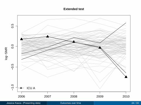
Extending the test to account for previous performance

Accounts for regression-to-the-mean over more than one period• A longer history of performance indicators are used to calculate

the baseline from which to measure the change.• When KPIs are quite variable, less likely to identify providers as

having deteriorated when this test is used.• KPIs quite variable implies low correlation between KPIs over time.


−1.

0−

0.5

0.0

0.5

Adjusted test

Year

log−

SM

R

ICU A

2006 2007 2008 2009 2010


−1.

0−

0.5

0.0

0.5

Extended test

Year

log−

SM

R

ICU A

2006 2007 2008 2009 2010


−1.

0−

0.5

0.0

0.5

Simple test

Year

log−

SM

R

●

ICU AICU B

2006 2007 2008 2009 2010

●

●

●

●

●

●

●

●

●

●

●

●

●

●

●

●

●

●

●

●

●

●

●

●

●

●

●

●

●

●

●

●

●

●

●

●

●

●

●

●

●

●

●

●

●

●

●

●

●

●

●

●

●

●

●

●

●

●

●

●

●

●

●

●

●

●

●

●

●

●

●

●

●

●

●

●

●

●

●

●

●

●

●

●

●

●

●

●

●

●

●

●

●

●

●

●

●

●

●

●

●

●

●

●

●

●

●

●

●

●

●

●

●

●

●

●

●

●

●

●

●

●

●

●

●

●

●

●

●

●

●

●

●

●

●

●

●

●

●

●

●

●

●

●

●

●

●

●

●

●

●

●

●

●

●

●

●

●

−1.

0−

0.5

0.0

0.5

Adjusted test

Year

log−

SM

R

ICU A

2006 2007 2008 2009 2010

−1.

0−

0.5

0.0

0.5

Extended test

Year

log−

SM

R

ICU A

2006 2007 2008 2009 2010


−1.

0−

0.5

0.0

0.5

New baselines for extended test

Year

log−

SM

R

Adjusted baselineOriginal dataExtended baseline

2006 2007 2008 2009 2010


−1.

0−

0.5

0.0

0.5


Year

log−

SM

R


2006 2007 2008 2009 2010


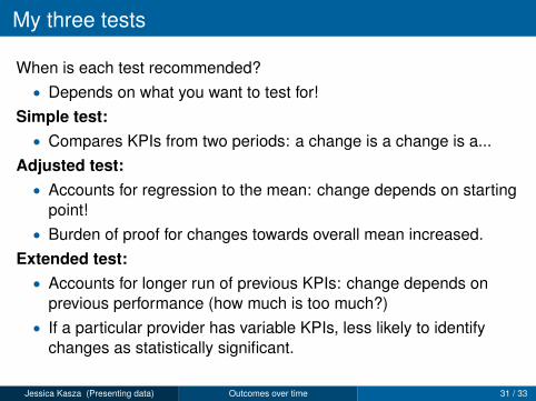
My three tests

When is each test recommended?• Depends on what you want to test for!

Simple test:• Compares KPIs from two periods: a change is a change is a...

Adjusted test:• Accounts for regression to the mean: change depends on starting

point!• Burden of proof for changes towards overall mean increased.

Extended test:• Accounts for longer run of previous KPIs: change depends on

previous performance (how much is too much?)• If a particular provider has variable KPIs, less likely to identify

changes as statistically significant.


Discussion: be careful what you test for...

• Testing for changes over time in the performance of providers ischallenging: a statistical approach is required!

• DON’T just look at raw changes in KPIs.• Statistical model for KPIs needs to be selected;• Appropriate statistical test needs to be chosen.

• Adjusted and extended tests (which account for previousperformance) are more ‘powerful’ than the simple test in certainsituations:

• Extended test most useful in detecting departures in performanceaway from the mean;

• Best when KPIs not too highly correlated (highly correlated⇒previous KPI good predictor of current KPI)

• If one of the tests is applied to a group of providers, issues ofmultiplicity should be considered.


References

• Cook DA, Coory M, Webster RA. Exponentially weighted movingaverage charts to compare observed and expected values for monitoringrisk-adjusted hospital indicators. BMJ Quality and Safety, 20:469–474,2011.

• Jones HE, Spiegelhalter DJ. Accounting for regression-to-the-mean intests for recent changes in institutional performance: Analysis andpower. Statistics in Medicine, 28:1645–1667, 2009.

• Kasza J, Moran JL, Solomon P. Evaluating the performance of Australianand New Zealand intensive care units in 2009 and 2010. Statistics inMedicine, 32:3720–3736, 2013.

• Kasza J, Moran JL, Solomon P. Assessing changes over time inhealthcare provider performance: addressing regression to the meanover multiple time points. Biometrical Journal, (to appear) DOI:10.1002/bimj.201400105.


Model for ICU log-SMRs

(Si2006, . . . ,Si2010)T ∼ N (µ,Σi)

• µ: population level of performance.• Variances, covariances of log-SMRs not constant over time or

from ICU to ICU.We assume µ = 0• Satisfied since year is included in patient-level mortality model.• Population-level drifts in performance not of interest here.• In general, can be assumed by subtracting yearly means from

performance indicators.


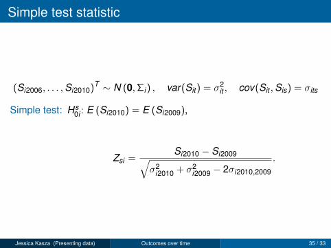
Simple test statistic

(Si2006, . . . ,Si2010)T ∼ N (0,Σi) , var(Sit ) = σ2it , cov(Sit ,Sis) = σits

Simple test: Hs0i : E (Si2010) = E (Si2009),

Zsi =Si2010 − Si2009√

σ2i2010 + σ2

i2009 − 2σi2010,2009

.


Adjusted test statistic

Regression-to-the-mean may need to be accounted for (Jones &Spiegelhalter, 2009)

Adjusted test: Ha0i : E (Si2010) = E (Si2010|Si2009),

Zai =Si2010 − E (Si2010|Si2009)√

var {Si2010 − E (Si2010|Si2009)}.

‘Adjusted’ baseline from which to measure the change: danger ofover-interpretation of Si2010 − Si2009.


Extended test statistic

Extended test: He0i : E (Si2010) = E (Si2010|Si2009, . . . ,Si2006)

Zei =Si2010 − E (Si2010|Si2009, . . . ,Si2006)√

var {Si2010 − E (Si2010|Si2009, . . . ,Si2006)}

Also developed the generalized test statistic: compare linearcombinations of performance indicatorse.g. average performance indicators over 2010 and 2009 to previousperformance indicators.


Simple model for power calculations

Si0 = τγi − σδi0 + Ui + εi0

Si1 = τγi + Ui + εi1

Si2 = τγi + σδi2 + Ui + εi2

Ui ∼ N(0, τ2)

εit ∼ N(0, σ2)

• γi : ‘true’ baseline level of performance;• δi2: change between periods 1 and 2;• δi0: change between periods 0 and 1.• All parameters assumed known.Si0

Si1Si2

∼ N

τγi − σδi0τγi

τγi + σδi2

,

σ2 + τ2 τ2 τ2

τ2 σ2 + τ2 τ2

τ2 τ2 σ2 + τ2

.

Expressions for the distributions of the simple, adjusted and extendedtests available.


Distributions of the test statistics

Simple: Zsi |δi2 ∼ N(δi2√

2,1)

Adjusted: Zai |δi2, γi ∼ N

(δi2 + γi

√ρ(1− ρ)√

ρ+ 1,1 +

ρ(ρ− 1)

ρ+ 1

)

Extended: Zei |δi2, γi , δi0 ∼ N(µZei ,1 +

ρ(ρ− 1)

(2ρ+ 1)(ρ+ 1)

),

µZei =

√1 + ρ

1 + 2ρ

(δi2 + δi0

ρ

ρ+ 1

)+ γ

√ρ(1− ρ)

(1 + ρ)(1 + 2ρ)

Correlation coefficient:

ρ =τ2

σ2 + τ2


Power of the test statistics

−3 −2 −1 0 1 2 3

0.0

0.2

0.4

0.6

0.8

1.0

ρ = 0.5, γ = 0

δ2

Pow

er

−3

−2

−1

0

1

23


Power of the test statistics

−3 −2 −1 0 1 2 3

0.0

0.2

0.4

0.6

0.8

1.0

ρ = 0.2, γ = −3

δ2

Pow

er

−3−2−10123

−3 −2 −1 0 1 2 3

0.0

0.2

0.4

0.6

0.8

1.0

ρ = 0.5, γ = −3

δ2

Pow

er

−3−2

−1

0

1

2

3

−3 −2 −1 0 1 2 3

0.0

0.2

0.4

0.6

0.8

1.0

ρ = 0.8, γ = −3

δ2

Pow

er

−3

−2

−1

0

1

2

3

−3 −2 −1 0 1 2 3

0.0

0.2

0.4

0.6

0.8

1.0

ρ = 0.2, γ = 0

δ2

Pow

er

−3−2−10123

−3 −2 −1 0 1 2 3

0.0

0.2

0.4

0.6

0.8

1.0

ρ = 0.5, γ = 0

δ2

Pow

er

−3

−2

−1

0

123

−3 −2 −1 0 1 2 3

0.0

0.2

0.4

0.6

0.8

1.0

ρ = 0.8, γ = 0

δ2

Pow

er

−3

−2

−1

0

1

23

−3 −2 −1 0 1 2 3

0.0

0.2

0.4

0.6

0.8

1.0

ρ = 0.2, γ = 3

δ2

Pow

er

−3−2−10123

−3 −2 −1 0 1 2 3

0.0

0.2

0.4

0.6

0.8

1.0

ρ = 0.5, γ = 3

δ2

Pow

er

−3

−2−10123

−3 −2 −1 0 1 2 3

0.0

0.2

0.4

0.6

0.8

1.0

ρ = 0.8, γ = 3

δ2

Pow

er

−3

−2

−1

0123


Application to ICU data

For each ICU, i = 1, . . . ,79, test:• Hs

0i : E (Si2010) = E (Si2009)

• Ha0i : E (Si2010) = E (Si2010|Si2009)

• He0i : E (Si2010) = E (Si2010|Si2009, . . . ,Si2006)

• Hg0i : E

(Si2010+Si2009

2

)= E

(Si2010+Si2009

2 |Si2008, . . . ,Si2006

).

In general, the most appropriate test would be selected and applied toall providers.


Type I error of tests

0.0 0.2 0.4 0.6 0.8 1.0

0.2

0.4

0.6

0.8

1.0

rho

P(t

yp

e I

err

or)

simple test statistic, adjusted test, extended test (2previous performance indicators conditioned on), extended test(3 previous PIs conditioned on), extended test (4 previous PIsconditioned on).


Controlling false discovery rate

0.0 0.2 0.4 0.6 0.8 1.0

0.0

0.2

0.4

0.6

0.8

rho

Fa

lse

dis

cove

ry r

ate

simple test statistic, adjusted test, extended test (2previous performance indicators conditioned on), extended test(3 previous PIs conditioned on), extended test (4 previous PIsconditioned on).


Outcomes over time: presenting data and testing for changes · Outcomes over time: presenting data...

Documents

Transcript of Outcomes over time: presenting data and testing for changes · Outcomes over time: presenting data...