OTTO VON-GUERICKE-UNIVERSITY AGDEBURG · Otto-von-Guericke-University Magdeburg Faculty of...

Setup Cost Reduction and Supply Chain Coordination in Case of Asymmetric

Information

Karl Inderfurth Guido Voigt

FEMM Working Paper No. 16, July 2008

OTTO-VON-GUERICKE-UNIVERSITY MAGDEBURG FACULTY OF ECONOMICS AND MANAGEMENT

F E M M Faculty of Economics and Management Magdeburg

Working Paper Series

Otto-von-Guericke-University Magdeburg Faculty of Economics and Management

P.O. Box 4120 39016 Magdeburg, Germany

http://www.ww.uni-magdeburg.de/

http://www.ww.uni-magdeburg.de/

Setup Cost Reduction and Supply Chain Coordination in

Case of Asymmetric Information

Karl Inderfurth∗ Guido Voigt†

Otto-von-Guericke-University Magdeburg

Faculty of Economics and Management

POB 4120, 39016 Magdeburg, Germany

July 11, 2008

Abstract

Screening contracts are a common approach to solve supply chain coordination

problems under asymmetric information. Previous research in this area shows that

asymmetric information leads to supply chain coordination deficits. We extend the

standard framework of lotsizing decisions under asymmetric information by allowing

investments in setup cost reduction. We find that asymmetric information leads to

an overinvestment in setup cost reduction. Yet, the overall effect on supply chain

performance is ambiguous. We show that these results holds for a wide variety of

investment functions.

∗Chair in Production Management and Logistics, [email protected]†Chair in Production Management and Logistics, [email protected]

1

1 INTRODUCTION

1 Introduction

The model utilized in this paper captures a supply chain planning problem, in which the

buyer asks the supplier to switch the delivery mode to Just-in-Time (JiT). We characterize

the JiT mode with low order sizes.

The buyer faces several advantages from a JiT-delivery, such as lower opportunity costs

(mainly for capital lockup), less inventory handling, storage room and handling equipment

as well as less rework and scrap. Additionally, JiT allows for a more even workload (and

therefore less idle time and more efficient production and material handling) and for less

complexity for production planning and control (see Schonberger and Schniederjans [25]).

However, we abstract from these multidimensional advantages and aggregate them to the

buyer’s holding costs. Hence, if the buyer faces high holding costs she is supposed to have

high advantages from a JiT-delivery, and vice versa.

On the other hand, smaller order sizes can cause an increase of the suppliers setup, holding

and distribution costs (see Fandel and Reese [8]). In our modelling approach, the supplier’s

setup costs per period reflect this disadvantages.

Yet, it is well known that small order sizes are not sufficient for a successful implementation

of the JiT concept. Setup cost reduction, thus, is regarded to be one main facilitator for

JiT to be efficient. Our model depicts the need for accompanying process improvements

by the supplier’s option to invest in setup cost reduction. Porteus [23] initially analyses

the potential benefits of setup cost reduction in the economic order quantity-framework.

Consecutive research often concentrates on the specific form of the investment function in

either the economic order or economic production quantity model (e.g. van Beek and van

Putten [28], Hahn et al. [11] , Kim [14]). Leschke [15] reviews this stream of research and

2

1 INTRODUCTION

conducts an empirical study to investigate a realistic shape of the investment function.

Other authors extend Porteus initial work by considering stochastic lead times (and de-

mand) or backorders (see Paknejad and Affisco [21], Keller and Noori [13] and Nasri et al.

[20]). An extension to the case of two stage systems and full information availability was

made by Paknejad, Nasri and Affisco [22]. This framework also was utilized to incorpo-

rate quality aspects in the suppliers‘ decision problem (see Affisco et al. 2002 [1], Liu and

Cetinkaya [17]). Our paper contributes to this stream of research by analysing the impact

of asymmetric information on the investment in setup cost reduction in a two stage supply

chain.

From a supply chain perspective, an implementation of a JiT strategy is only profitable,

if the buyer‘s cost advantages exceed the supplier‘s cost increase. Yet, previous research

states that this is not always the case.1 The supplier, thus, may have a strong incentive to

convince the buyer to abandon the JiT strategy. However, as the buyer is supposed to be

in a strong bargaining position (as it is, for instance, often the case in the automotive in-

dustry), he will not be convinced unless he is offered a compensation for the disadvantages

of not implementing the JiT strategy. Yet, as long as there is a lack of coordination (i.e.

as long as pareto improvements are possible by reducing the total supply chain’s cost),

the supplier can compensate the buyer while improving his own performance.

1Myer [19] finds that a buyer’s single-handed JiT implementation causes a supply chain cost increase

of 25% to 30% in the food industry (basically due to transportation, warehousing, unnecessary one-to-one

communication on the sales side, as well as ineffective promotion and advertising on the marketing side),

and a cost increase in the range of 10% to 20% in other consumer goods fields. In these cases, the buyer’s

isolated JiT decision obviously leads to a lack of supply chain coordination due to the supplier‘s cost

increase.

3

1 INTRODUCTION

Nonetheless, the above-mentioned advantages of a JiT strategy are multidimensional and

contain to a major extent private information of the buyer. Thus, they can certainly not

be easily observed and valued by the supplier. Of course, the supplier may ask the buyer

about the disadvantages of abandoning the JiT strategy (or as the case may be how much

compensation he demands to abandon the JiT strategy). However, the buyer will appar-

ently claim that switching towards higher order sizes causes substantial costs and that a

high compensation is required.

Assuming the strategic use of private information, it is in the supplier’s best interest to

offer a menu of contracts (i.e. screening contract) (see [Corbett and de Groote [5],Ha

[10], Corbett [4],Corbett and Tang [6],Corbett et al. [7], and Sucky [27]]). Basically, this

menu of contracts aligns the incentives of the supply chain members such that a buyer

with low advantages of a JiT delivery will agree upon higher order sizes than a buyer with

high advantages of this supply mode. One main result which stems from the screening

literature is that asymmetric information leads to inefficiencies, because the resulting or-

der sizes are too low compared to the supply chain’s optimal solution. Starting from this

insight, our main focus in this study is to analyse the impact of investments in setup cost

reduction on this lack of coordination. Specifically, we are interested in investigating if

the supplier’s option to reduce his setup cost and, thereby decrease his lotsize, might lead

to an improvement in supply chain coordination. If a complete cut of setup costs could be

achieved at no (or very minor) cost, the supplier would offer an JiT contract and perfect

coordination would take place. However, the impact of costly setup cost reduction on

supply chain coordination is not clear at all.

Summing up, there are basically two streams of research (namely the inefficiencies due to

4

2 OUTLINE OF THE MODEL

asymmetric information and the optimal set-up cost reduction in an integrated lot-sizing

decision) this paper combines.

2 Outline of the model

S u p p l i e r B u y e r

Figure 1: Supply Chain

This paper analyses a simplified Joint-Economic-Lotsizing model [see Goyal [9],Monahan

[18]and Banerjee [2]]. In a dyadic relationship, composed of a buyer (B) and a supplier

(S), the buyer decides upon the order lotsize (Q) from her supplier. Let f denote the setup

costs for each delivery incurred by the supplier. This setup costs are a decision variable

for the supplier’s decision problem. The cost for reducing the setup costs from its original

level fmax by fmax − f,∀f ≥ fmin ≥ 0 are captured by the investment function k(f). The

investment k(f) leads to a setup cost reduction over the whole (infinite) planning horizon.

Hence, the supplier faces costs of r · k(f) in each period, where r denotes the company

specific interest rate.2 The buyer faces holding costs h per item and period. The demand

is, without loss of generality, standardized to one unit per period. Hence period costs

equal unit costs. Lot-for-Lot production is assumed on the supplier’s side. The following

situation is considered, with the buyer as the focal player in the supply chain. She asks the

supplier to deliver a product Just-in-Time (JiT). As the supplier is in a weak bargaining

position, he either delivers JiT or he offers a contract which makes the buyer as well off

2If the time horizon is finite, r can be interpreted as the annuity factor. In this case, a constant order

size Q is (ceteris paribus) still optimal [see Brimberg and Hurley [3]].

5


as she would be by sourcing from an alternative JiT supplier. Obviously, both options

can be accompanied by an investment in setup cost reduction. We show in the following

how the supplier can optimally convince the buyer to accept higher order sizes even if the

buyer’s advantages of the JiT delivery can only be estimated.

Full Information If the supplier knows the buyer’s holding costs h, he offers the fol-

lowing contract, consisting of order size Q, side payment T and the corresponding setup

cost f , to minimize his period costs KS . The buyer has the outside option to buy from

an alternative supplier (AS) who delivers in a JiT mode. The cost of buying from the

alternative supplier is CAS per unit. To induce higher order sizes while ensuring that the

buyer does not choose her outside option, the supplier must compensate the buyer for the

additional holding cost with a side payment T per unit (e.g. by introducing a quantity

discount on the wholesale price). The supplier’s optimal contract is the outcome of the

following optimization problem:

Problem FI

minKS(Q, T, f) =f

Q+ T + r · k(f)

s.t.

h

2Q − T ≤ CAS (PC)

fmin ≤ f

f ≤ fmax

It is easy to see that the participation constraint (PC) needs to be binding for an optimal

solution. Substituting T = h2Q − CAS in the objective function, and setting up the

6


Lagrange-function gives:

L(Q, f, α, γ) =f

Q+

h

2Q − CAS + r · k(f)

+ α(fmin − f) + γ(f − fmax).

The solution of minQ,f,α,γ

L(Q, f, α, γ) gives the (supply chain optimal) contract parame-

ters Q(SC)∗ and T (SC)∗, the optimal investment level f(SC)∗ and the optimal la-

grange parameters α(SC)∗, γ(SC)∗, i.e. the order quantity Q(SC)∗ causes the lowest

possible cost for the overall supply chain. The supply chain optimal order size is the

well known economic order quantity (EOQ) with respect to the reduced setup costs, i.e.

Q(SC)∗ =

√

2·f(SC)∗

h. Kim et al. [14] show that the optimal setup cost level f(SC)∗

of problem FI is dependent on the shape of the total cost function. They also give an

optimization procedure for any investment function k(f). These results can easily be

integrated in our framework. Particularly, they show that for a concave and a linear in-

vestment function the optimal investment level f(SC)∗ is either fmin (⇒ α(SC)∗ 6= 0) or

fmax (⇒ γ(SC)∗ 6= 0). For a convex investment function the optimal investment level is

either an interior solution (i.e. α(SC)∗ = 0 and γ(SC)∗ = 0) or a corner solution (i.e.

α(SC)∗ 6= 0 or γ(SC)∗ 6= 0). In the following, we extend the framework to the case of

asymmetric information and analyse the influence on supply chain coordination.

S u p p l i e r o f f e r s m e n u o f c o n t r a c t s

B u y e r c h o o s e s o n e c o n t r a c t

o u t o f t h e m e n uS u p p l i e r d e c i d e s u p o nt h e i n v e s t m e n t i n

s e t u p c o s t r e d u c t i o n

Figure 2: Decision sequence

7


Asymmetric Information As mentioned in the introduction, the buyer’s several ad-

vantages from a JiT delivery are captured by an aggregated measure, namely her holding

costs. As full information about all these JiT related advantages is a very critical as-

sumption we study a situation where the buyer is only able to estimate these advantages.

We formalize this estimation with a probability distribution pi(hi) (i = 1, ..., n) over all

possible holding cost realizations hi. Common knowledge of the probability distribution

pi(hi) is assumed.

One feasible solution to this problem with respect to the buyer’s participation constraint

(PC) can be obtained by solving it as if under full information (FI) with h = hn. How-

ever, this solution is not optimal for the supplier as he can increase his expected profits by

offering a menu of contracts Qi, Ti (i = 1, ..., n), which the buyer can choose from. Figure

2 illustrates the decision sequence. The optimal menu of contracts (Q∗i , T

∗i ∀i = 1, ..., n)

is the solution to the following optimization problem :

Problem AI

minE(KS(fi, Qi, Ti)) =n∑

i=1

pi

(

fi

Qi+ Ti + r · k(fi)

)

∀i = 1, ..., n

s.t.

hi

2Qi − Ti ≤ CAS (PC) ∀i = 1, ..., n

hi

2Qi − Ti ≤

hi

2Qj − Tj (IC) ∀i 6= j; i, j = 1, ..., n

fi ≤ fmax ∀i = 1, ..., n

fmin ≤ fi ∀i = 1, ..., n

8


The incentive constraint (IC) ensures that the buyer with holding costs hi incurs the lowest

possible cost per period when choosing the order size Qi. Hence, the cost minimizing buyer

reveals her holding cost through the contract choice. The participation constraint (PC)

ensures that no buyer, regardless of her holding costs, will choose the alternative supplier

(AS).

Setting up the Lagrange-function gives:

L(Qi, Ti, fi, λij , µi, γi, αi | i, j = 1, ..., n and i 6= j) =

n∑

i=1

pi

(

fi

Qi+ Ti + r · k(fi)

)

+n∑

i=1

µi(hi

2Qi − CAS − Ti)

+n∑

i=1

n∑

j=1,j 6=i

λij(hi

2Qi − Ti −

hi

2Qj + Tj) +

n∑

i=1

αi(fmin − fi)

+

n∑

i=1

γi(fi − fmax)

The interested reader can find the Karush-Kuhn-Tucker (KKT) conditions for an optimal

solution in Appendix 6.1. The optimal solution to the problem AI gives the optimal menu

of contracts Q∗i , T

∗i , the optimal investment level f∗

i and the optimal lagrange parameters

µ∗i , α

∗i , γ∗

i and λ∗ij . The corresponding supply chain optimal order size (i.e. the order size

that solves problem FI with h = hi) is denoted by Q∗i (SC).

In the optimal screening contract, the order sizes increase with decreasing holding costs

(i.e. Q∗i−1 ≥ Q∗

i , ∀i = 2, ..., n) and the side payments increase respectively (i.e. T ∗i−1 ≥

T ∗i , ∀i = 2, ..., n). Please note that for certain combinations of probabilties pi(hi), i =

1, ..., n and holding costs hi, i = 1, ..., n the order size relation Qi−1 = Qi may hold in the

optimal menu of contracts. In this case, there is no information revelation through the

buyer’s contract choice (as the supplier cannot distinguish the buyer facing holding cost

9


hi−1 from the buyer facing holding cost hi). Yet, in the screening literature it is common to

rule out this cases by imposing a restriction on the probabilty distribution.3 We follow this

approach and ,thus, restrict our analysis of the settings in which information relevation

is prevalent, as this is the main feature of screening models. We exclude the cases of no

information relevation by assuming that the following condition between probabilities and

holding costs hold:

hi +

∑i−1t=0 pt

pi(hi − hi−1) < hj +

∑j−1t=0 pt

pj(hj − hj−1) (1)

∀ i = 1, ..., n − 1; j = 2, ..., n; j > i and p0, h0 = 0

This condition is always satisfied if there are only two possible holding cost realizations

because p0 = 0, p1 > 0 and h1 < h2 holds. However, if the supplier faces more than

two possible holding cost realization, there exist combinations of pi and hi for which (1)

does not hold and information revelation would not be observable for every holding cost

parameter hi. The optimality conditions for the optimal menu of contracts in these cases

are specified in Spence [26]. However, assumption (1) has no impact on the main results

in this study but simplifies the derviation of the suppliers optimal decision.

Furthermore, the resulting order sizes are too low compared to the supply chain optimum

(i.e. Q∗i < Qi(SC)∗ for all i = 2, ..., n) except the ordersize Q∗

1. Hence, there is a lack of

supply coordination except for the buyer facing the lowest possible holding costs.

Finally, the buyer with holding costs hi is indifferent between the contracts Q∗i , T

∗i and

Q∗i+1, T

∗i+1 (∀i = 1, ..., n−1), and the buyer facing the highest holding cost hn is indifferent

3In models with a continuous distribution over the private information a monotone hazard rate of the

probabilty distribution is normally assumed.

10

3 IMPACT ON SUPPLY CHAIN COORDINATION ANDPERFORMANCE

between the contract Q∗n, T ∗

n and the alternative supplier.4 Hence, information revelation

requires that the buyer facing holding costs hi chooses the order size Qi even though the

order size Qi+1 has the same cost impact for her. Thus, it is a common assumption within

the screening literature that the indifferent buyer chooses the order size which is in her

supplier’s best interest. We refer to Inderfurth et al. [12] for a discussion of this behavioral

assumption in screening models.

3 Impact on Supply Chain Coordination and Performance

In the following, we present the supplier’s optimal menu of contracts Q∗i , T

∗i and the

corresponding setup cost level f∗i . The optimal menu of contracts is derived from the

KKT-conditions (see Appendix 6.2, (36)-(40)):

Q∗i =

√

2 · f∗i

hi + φi∀i = 1, ..., n (2)

where φi =

∑i−1t=0 pt

pi(hi − hi−1) ∀ i = 1, ..., n and p0, h0 = 0 (3)

T ∗n =

hn

2Q∗

n − CAS (4)

T ∗i =

hi

2(Q∗

i − Q∗i+1) + T ∗

i+1 ∀i < n (5)

The optimal setup costs f∗i results from solving (see Appendix 6.2, (42))

√

hi + φi

2 · f∗i

= −r ·dk(fi)

dfi

∣

∣

∣

∣

fi=f∗i

(6)

4For a derivation and a broader discussion of the optimal menu of contracts’ properties we refer to

Sappington [24] or Spence [26].

11


as long as the optimal setup cost level is an interior solution. Otherwise, the optimal setup

cost level is a corner solution (i.e. fmin or fmax).

Obviously, the supplier takes the option of setup cost reduction into consideration when

offering the menu of contracts. Hence, his decision in the third stage (see figure 2) is

already considered in the first stage. Otherwise, he would offer suboptimally high order

sizes as (2) is dependent on f∗i , and f∗

i is computed from (6).

Distortionary effects of asymmetric information

As already mentioned in section 2, asymmetric information leads to supply chain ineffi-

ciencies caused through a downward distortion in order sizes. One can easily see from (2)

that φi makes the difference compared to the EOQ-formula (i.e. the supply chain optimal

solution). Hence, analysing the distortion caused by asymmetric information reduces to

analysing φi. Hence, the higher φi the higher Qi(SC)∗ − Q∗i , i.e. the distortion increases

with increasing φi.

The distortion, thus, increases with an increasing ratio∑

i−1

t=0pt

pi. The higher this ratio, the

higher the probability that the buyer will choose an order size Qk, k < i due to the screen-

ing. Hence, the expected cost minimizing supplier will decrease (the less likely choosen

order size) Qi as he can decrease the side payments Tk for all k ≤ i (see (4),(5)) as well.

The order size deviation from the supply chain optimum (Qi(SC)∗ − Q∗i ) therefore in-

creases.

Furthermore, the distortion depends on the distance between hi and hi−1. Intuitively,

there are no asymmetric information if the difference of the respective holding costs is

zero. Thus, the asymmetry of information (and therefore the distortion) increases the

more different the respective holding costs.

12


k ( f )

ff m i n f m a x

l i n e a r

c o n v e x

c o n c a v e

Figure 3: Progressive shapes of the analysed investment functions

In the following, we will analyse whether asymmetric information leads to a distortion

of the buyer’s investments in setup cost cost reduction. The analysis is carried out for

convex, concave and linear investment functions. Figure 3 depicts the shape of the anal-

ysed investment functions.5 We will utilize the KKT-conditions and therefore a marginal

approach to derive our results. This approach seems reasonable since an intutive graphical

representation of the analysed problem is possible. However, the interested reader finds

another intuitive approach for the problem under full information in Kim et al [14].

13


f min f max

marginal revenue

>

marginal costs

f i

TM(f i )

marginal revenue

<

marginal costs

MR(f i )

MC( f i )

1

2 f r

Figure 4: Optimal investment level given a concave investment function

3.1 Concave and linear investment function

From the evaluation of the KKT-condition in (6) we get√

hi+φi

2·f∗i

= −r · dk(fi)dfi

∣

∣

∣

fi=f∗i

, as long

as α∗i = 0, γ∗

i = 0, i.e. as long as the optimal setup cost level is an interior solution. Hence,

only a setup cost level fi which satiesfies this condition is an interior solution. Next we

will show, however, that this solution is a cost maximum instead a cost minimum. Thus,

a corner solution will result in the cost minimum.

Let MR(fi) =√

hi+φi

2·fidenote the marginal revenues and MC(fi) = −r· dk(fi)

dfithe marginal

costs for reducing the setup cost level fi. Figure 4 depicts MC(fi), MR(fi) and TM(fi) =

MR(fi) − MC(fi).

As the MC-curve is monotonically increasing for a concave investment function (d2k(f)d2f

<

5We refer to Leschke and Weiss [16] for a review of commonly assumed investment functions. The

convex followed by the the linear investment function is most commonly assumed.

14


0 → −d2k(f)d2f

> 0), the TM -curve is strictly monotonically decreasing (and there is at most

one interior solution). Yet, we need to consider the integral over TM(fi) to evaluate the

profitability of a setup cost reduction. Let fr denote the root of TM(fi) (i.e. the interior

solution to problem AI). If fr ∈ (fmin, fmax), a reduction of setup costs to fr causes a

loss of∫ fmax

frTM(fi)dfi (i.e. area 2).6 Hence, fr is a local cost maximum. As TM(fi)

is strictly monotonically decreasing, a setup cost reduction beyond fr leads to profits of

∫ fr

fminTM(fi)dfi (i.e. area 1). Hence, if TM intersects the abscissa between fmin or fmax,

the optimal investment level depends on the ratio of the areas 1 and 2. If 1 is bigger than

2, then the optimal setup level is fmin, otherwise it is fmax. Therefore, α∗i > 0 or γ∗

i > 0

holds. Figure 4 depicts the case, in which the optimal setup cost level is fmin.

The same argument holds for a linear investment function (see figure 5). As MC(fi)

is constant, TM(fi) is strictly monotonically decreasing. Hence, there is at most one

intersection with the abscissa. Therefore, the optimal setup cost level is a corner solution

as well (i.e. fmin or fmax). Therefore, α∗i > 0 or γ∗

i > 0 holds. Figure 5 depicts the case,

in which area 2 is bigger than area 1. Hence, no setup cost reduction at all is profitable.

These results are in line with the findings in Kim et al [14]. Under full information, thus,

this would be the optimal solution. Now, however, we consider the impact of asymmetric

information on the investment decision. In (6) we see that the marginal revenue increases

with increasing φi.

From φi =∑

i−1

t=0pt

pi(hi − hi−1) ≥ 0 follows that the MR-curve under full information is be-

neath the MR-curve under asymmetric information. Let TMFI(fi) denote the difference

6Please note that figure 4 depicts the setup cost level fi instead of the setup cost reduction fmax − fi.

Hence, the higher the setup cost reduction the lower the setup cost level (i.e. fi is closer to the point of

origin).

15


f min f max

marginal revenue

>

marginal costs

f i

TM(f i )

marginal revenue

<

marginal costs

MR(f i )

MC(f i )

1

2

f r

Figure 5: Optimal investment level given a linear investment function

between marginal revenue and marginal cost under full information and TMAI(fi) under

asymmetric information respectively. It follows directly that TMFI(fi) ≤ TMAI(fi), ∀ fi.

Hence, area 1 increases and area 2 decreases in size due to asymmetric information. If

the supply chain optimal investment level is f∗i (SC) = fmax (i.e. area 1 < area 2), and

the optimal investment level under asymmetric information is f∗i = fmin (i.e. area 1 >

area 2) there is an overinvestment in setup cost reduction. Figure 6 depicts this case. The

same arguments holds for a linear investment function. Hence, asymmetric information

can lead to an overinvestment in setup cost reduction.

3.2 Convex investment function

Now we consider the distortionary effect of asymmetric information on the setup cost

investment level in case of a convex investment function. Yet, as both MR(fi) and MC(fi)

16


f min f max

f i

TM FI (f i )

MR FI (f i )

MC(f i )

MR AI (f i )

TM AI (f i )

1

2

Figure 6: Overinvestment in case of a concave investment function

are monotonically decreasing (d2k(f)d2f

> 0), it is not clear whether TM(fi) is monotonic

at all. Figure 7 shows the case of a) a monotonically increasing TM -curve and b) a

monotonically decreasing TM -curve. If the TM -curve is not monotonic at all, there are

multiple interior solutions. However, the argumentation in this situation can either be

reduced to case a) or b).

For case b) the same argument as for the concave and linear investment function holds

(i.e. there is at most one cost maximum). Hence, the optimal setup cost level is either

fmin or fmax, and there is also the possibility of an overinvestment due to asymmetric

information.

Yet, as long as TM(fi) is strictly monotonically increasing (case a), the optimal investment

is

17


f∗i =

fr , if fr ∈ [fmin, fmax]

fmin , if fr < fmin

fmax , else

. (7)

This is because all setup cost reductions beyond fr are not profitable. Hence, in contrast

to a concave or linear investment function, fr results in a cost minimum instead a cost

maximum.

Next, we consider the effect of asymmetric information. As long as the order sizes change

due to a screening (i.e. MRAI(fi) > MRFI(fi)) and the optimal setup cost level is not

a corner solution there is an overinvestment in setup cost reduction. Figure 8 illustrates

this case.

Yet, if TM(fi) is not monotonic at all, the same arguments as for the separated cases a)

and b) in figure 7 hold. Hence, also in this situation, an overinvestment is possible if the

investment decision changes due to an upward-shift of TM(f) (i.e. due to asymmetric

information).

As such, one can summarize that there is always the possibility of an overinvestment in

setup reduction, regardless of the actual shape of the investment function. This result

is basically driven by the fact that the supplier’s screening regarding the buyer’s private

information leads to order sizes which are smaller than the supply chain optimal order sizes

(i.e. Q∗i < Q∗

i (SC),∀i = 2, ..., n, see section 2). This leads to higher marginal revenues

from the investment in setup cost reduction. Yet, it is not obvious whether the coordination

deficit (i.e. the performance gap between supply chain optimum and screening contract)

is increasing or decreasing due to an investment in setup cost reduction, as there are two

18

4 THE POWER COST FUNCTION CASE

contrary effects:

Overinvestment effect. As stated in section 3, an overinvestment in setup cost reduc-

tion due to asymmetric information is likely. Yet, from a supply chain perspective, this

overinvestment causes a coordination deficit.

Setup cost effect. As shown in section 2, the coordination deficit due to asymmetric

information is essentially caused by a deviation from the supply chain optimal order quan-

tity (i.e. Q∗i ≤ Q∗

i (SC)). Therefore, there is no supply chain optimal trade-off between

holding costs and setup costs per period.7 The setup costs per period are suboptimally

high and the holding costs suboptimally low. Yet, as there is the option to invest in setup

cost reduction (and even an overinvestment is possible), this unbalanced trade-off carries

less weight. The setup cost effect, thus, measures the isolated coordination gains from

reducing the setup cost while disregarding the investment costs.

In the following section, we conduct a numerical study for two possible holding cost realiza-

tion to analyse the impact of the overinvestment- and setup cost effect on the coordination

deficit.

4 The Power Cost Function Case

In the following, we illustrate the previous analysis for Porteus “Power Cost Function

Case“ [23] as an example for a convex investment function. If this investment function

7In the classical economic lotsizing model, the fixed- and holding costs per period are equal in the

optimum. Yet, lower order sizes due to asymmetric information lead to fixed cost per period that are

higher than the holding costs per period.

19


f min f max

MR(f i )

MC(f i )

TM(f i )

f min f max

MR(f i )

MC(f i )

TM(f i )

b) a)

f i f i f r f r

Figure 7: Optimal investment level in case of a convex investment function

f min f max

MR FI (f i )

MC(f i )

TM FI (f i )

MR A I (f i )

f i * f i (SC) *

Overinvestment

TM A I (f i )

f i

Figure 8: Overinvestment in case of a concave investment function

20


is utilized, decreasing marginal percentage returns are presumed. Therefore, the supplier

faces investment costs in the amount of ki(f) = a · f−b − d ∀a, b, d, f > 0 if he reduces

the setup costs from the initial value of fmax to f , where f > fmin = 0. Let c denote the

costs of reducing the setup cost fmax by π%, then an additional reduction by π% results

in an investment of (1 + β) · c. Then, the investment function has the following shape:

ki(fi) = a · f−bi − d with b = −ln(1+β)

ln(1−0,01π) ,a = c·fbmax

(1−0,01π)−b−1and d = a · f−b

max .

Full Information:

In the following we restrict our analysis on n = 2 (i.e. h ∈ [h1, h2]). Then, the optimal

contract parameters under full information are

Q∗(SC) = min

(√

2fmax

h,

(

2

h

) b

2b+1(

2abr

h

) 1

2b+1

)

(8)

f∗(SC) = min

(

fmax,

(

2(abr)2

h

)1

2b+1

)

(9)

[see Porteus [23]].

Asymmetric Information

The optimal contract parameters for two possible holding cost realizations h1 and h2 are

(see Appendix 6.3):

f∗2 =

fr , if fr ∈ [fmin, fmax]

fmin , if fr < fmin

fmax , else

(10)

where fr =

(√

2

hi + φ2· r · a · b

)( 1

b+0.5)

(11)

(12)

21


Q∗2 =

√

2 · f∗2

h2 + φ2(13)

T ∗2 =

h2

2Q∗

2 − CAS (14)

where φ2 =p1

p2(h2 − h1) (15)

f∗1 = f1(SC)∗ = min

(

fmax,

(

2(abr)2

h1

)1

2b+1

)

(16)

Q∗1 = Q1(SC)∗ = min

(

√

2 · fmax

h1,

(

2

h1

) b

2b+1(

2abr

h1

) 1

2b+1

)

(17)

T ∗1 =

h1

2(Q∗

1 − Q∗2) +

h2

2Q∗

2 − CAS (18)

4.1 Numerical example

Suppose β = 0.01, π = 10[%](⇒ b = 0.094), c = 25, fmax = 800 (⇒ a = 4700, d =

2500, ki(fi) = 4700 · f−0,094 − 2500), CAS = 2.5, fmin = 0, h1 = 1, h2 = 5, p1 = 0.5 and

p2 = 0.5. Let (Qfmax

i , Tfmax

i , i = 1, 2) denote the optimal menu of contracts with no

setup cost reduction possible. In this case, Qfmax

i (SC) , i = 1, 2 denotes the supply chain

optimal order quantity. Furthermore, Ki(SC)(Qi, fi) = fi

Qi+ hi

2 Qi + r(

af−b − d)

, i = 1, 2

denote the supply chain costs that result if the buyer faces holding costs hi. Finally,

E(K(SC)) =∑2

i=1 pi · Ki(SC) denote the expected supply chain costs. In the following

we concentrate our analysis on the overall supply chain. Hence, we do not list the side

payments Ti that correspond to the respective order size as these payments have no impact

on the overall supply chain.

If no setup cost reduction is possible, the optimal order sizes and respective supply chain

costs are

22


Qfmax

1 = 40 Qfmax

1 (SC) = 40

K1(SC)(Qfmax

1 , fmax) = 40 K1(SC)(Qfmax

1 (SC), fmax) = 40

Qfmax

2 = 13.33 Qfmax

2 (SC) = 17.89

K2(SC)(Qfmax

2 , fmax) = 93.34 K2(SC)(Qfmax

2 (SC), fmax) = 89.44

E(K(SC)(Qfmax

i , fmax) = 66.67

Yet, if setup cost reduction is feasible, the following optimal contract parameters and setup

costs result:

Q∗1 = 40 Q∗

1(SC) = 40

f∗1 = 800 f∗

1 (SC) = 800

K1(SC)(Q∗1, f

∗1 ) = 40 K1(SC)(Q∗

1(SC), f∗1 ) = 40

Q∗2 = 6.08 Q∗

2(SC) = 10.45

f∗2 = 166.6 f∗

2 (SC) = 273.15

K2(SC)(Q∗2, f

∗2 ) = 82.52 K2(SC)(Q∗

2(SC), f∗2 ) = 78.97

E(K(SC)(Q∗i , f

∗i )) = 61.26

Figure 11 in Appendix 6.4 depicts the marginal analysis from section 3 for the numer-

ical example. In the following, we analyse the impact of the option to invest in setup

cost reduction on the coordination deficit that arises due to asymmetric information. Ad-

ditionally, the effect of setup cost reduction on the overall supply chain performance is

analysed.

4.2 Coordination deficit and setup cost reduction

Let CD = K2(SC)(Q∗2(SC), f∗

2 (SC)) − K2(SC)(Q∗2, f

∗2 ) denote the coordination deficit

with the option to invest in setup cost reduction and

CDfmax = K2(SC)(Qfmax

2 (SC), fmax) − K2(SC)(Qfmax

2 , fmax) the coordination deficit

23


without the option to reduce setup costs.8 In the numerical example, the coordination

deficit decreases from CDfmax

= 3.9 to CD = 3.56. The changes in the coordination deficit

∆CD = CD − CDfmax

can be split into the overinvestment effect (OE) and the setup

cost effect (SE), i.e. ∆CD = OE − SE (please refer to Appendix 6.5 for a mathematical

formulation of ∆CD, SE and OE). When ∆CD > 0, the coordination deficit increases

due to an investment in setup cost reduction, and vice versa. The overinvestment effect

amounts to OE = 13.23 and the setup cost effect amounts to SE = 13.56. Hence, the

coordination deficit changes by ∆CD = 3.56− 3.9 = 13.22− 13.56 = −0.34 resulting in a

decrease of the coordination deficit due to setup cost reduction. Note that this reduction

completely benefits the supplier. In contrast, a positive ∆CD would completely increase

the supplier’s cost. The participation constraint in problem AI ensures that the buyer

with holding cost realization hn = h2 yields the same cost for all parameter values of the

problem. Hence, a change in the coordination deficit by ∆CD only affect the supplier’s

costs.

To investigate whether this result is robust against changing parameter values, we conduct

a comparative static analysis for all possible parameter values r. Please notice that even if

∆CD < 0, there would still be a coordination deficit. This deficit is always prevalent when

there is a deviation from the optimal order quantity due to screening. ∆CD only depicts

the effect of investments in setup cost reduction compared to no setup cost reduction.

Figure 9 depicts the changes of ∆CD in dependence of the interest rate r. The overinvest-

ment effect carries less impact, when the investment in setup cost reduction is inexpensive

8As there is no coordination deficit, if the buyer faces holding costs h1 we restrict the analysis to the

cases in which the buyer faces the holding costs h2.

24


(i.e. if the interest rate r is low). Yet, if r increases, the impact of the overinvestment effect

becomes predominant and the supply chain performance deteriorates. The impact of the

investment on supply chain performance is worst if r takes a value so that f∗2 (SC) = fmax

and γ(SC)∗ = 0 holds, i.e. if fmax is the interior solution to problem FI (r ≈ 0, 19).9 This

is the situation where overinvestment reaches its maximum. Beyond this interest rate r,

the total overinvestment fmax − f∗2 decreases. Hence, the overinvestment as well as the

setup cost effect decreases. Nonetheless, the overall effect on the supply chain performance

is negative. Please note that the coordination deficit vanishes if the setup cost reduction

is costless (i.e. r = 0) because the supplier will reduce the setup cost to the maximum

extend. Figure 14 in Appendix 6.6 shows that this coordination deficit reduction is ac-

companied by low order sizes Q∗2(SC) and Q∗

2. The supply chain, thus, tends to the JiT

mode if setup cost reduction is inexpensive. Furthermore, this figure points out that the

downward distortion of order sizes (i.e. Q∗2 ≤ Q∗

2(SC)), which is well known from other

screening models, continues to be responsible for the inefficiencies within the supply chain.

The interested reader can find more comparative static analyses for the parameters fmax,

h2 and π in Appendix 6.6, figure 12. Yet, the main result does not change for this analysis:

whether the investment in setup cost reduction reduces the coordination deficit or not

depends on the parameter values. As stated earlier, ∆CD directly affects the supplier’s

pay-offs. Yet, the coordination analysis is only conducted for the buyer with holding cost

h2. However, even if ∆CD > 0, the menu of contract Q∗i , T

∗i and the corresponding f∗

i is

optimal for a supplier with risk neutral preferences.

9This value results from solving (6) with f∗ = fmax = 800 and φ = 0 for r

25


Overinvestment

effect

Setup cost

effect

Monetary

units

0.25

20

0.0

r

0.3 0.1 0.05

10

15

0.2 0.15

0

5 max

f CD

CD

CD

Figure 9: Comparative static analysis w.r.t. r

4.3 Supply Chain performance and setup cost reduction

So far, we mainly concentrated on the coordination deficit and therefore on the abso-

lute inefficiencies that arise due to asymmetric information. However, an increase of the

supply chain deficit does not necessarily lead to a deterioration of supply chain perfor-

mance. To analyse the effect on the overall supply chain performance we compute the

expected change in supply chain costs that result if setup cost reduction is possible, i.e.

∆P = E(K(SC)(Qfmax

i , fmax) − E(K(SC)(Q∗i , f

∗i )). Hence, if ∆P < 0, the supply chain

performance deteriorates in the presence of setup cost reduction option due to asymmetric

information. Please note, that the supply chain performance will never decrease under full

information as no setup cost reduction is a feasible solution. In the numerical example the

26


expected supply chain performance increases by ∆P = 66.67 − 61.26 = 5.41. Hence, the

expected supply chain performance increases if the supplier reduces his setup costs. We

test again the robustness of this result for changing parameter values r.

Figure 10 illustrates the changes in supply chain performance in dependence from r. In

contrast to the results under full information the overall supply chain performance dete-

riorates due to setup cost reduction in some regions. The parameter values for which the

expected supply chain performance deteriorates are a subset of the parameter values for

which ∆CD > 0 holds. This is not suprising, as the supply chain performance can only

improve if the buyer faces holding costs h1. Nonetheless, the analysis of the changes in ex-

pected costs is important to evaluate the overall effect on the supply chain performance.10

The evaluation of ∆CD and ∆P , thus, implies different interpretation for the overall

supply chain. If the parameter values are such that ∆P < 0, then the option of setup

cost reduction harms the overall supply chain performance. In contrast, if ∆CD > 0 and

∆P > 0 holds, then the option of setup cost reduction improve the supply chain per-

formance, but the supply chain managers should be aware that cooperative and truthful

information sharing would have an even greater impact on improving supply performance

as if no setup cost reduction is possible. Finally, if CD < 0, then the coordination problem

due to asymmetric information lessens or even vanishes.

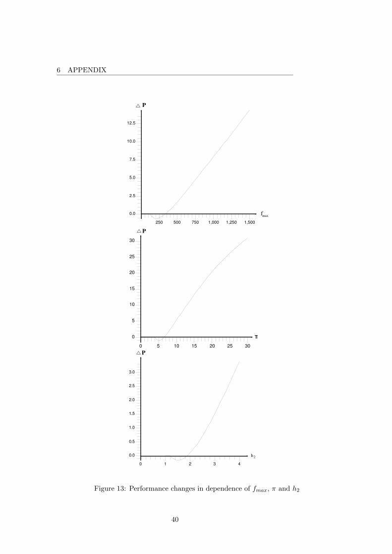
10The interested reader can find more comparative static performance analyses for the parameters fmax,

h2 and π in Appendix 6.6, figure 13. Again, the main result does not change for this analysis: whether the

investment in setup cost reduction reduces the supply chain performance or not depends on the parameter

values.

27

5 CONCLUSIONS

r

P

50

0.25

10

60

40

0.3

30

20

0

0.2 0.15 0.1 0.05

Figure 10: Changes in supply chain performance in dependence from interest rate r.

5 Conclusions

JiT delivery has received ever-increasing attention in the recent past. Typically, the imple-

mentation of JiT strategies is accompanied by setup cost reductions. If a weak bargaining

position of the supplier is presumed, the supplier’s optimal reaction is offering a pareto

improving menu of contracts if he only posseses imperfect information about the buyer’s

cost position. The analysis of setup cost reduction under asymmetric information shows

that the suppliers should take the option of setup cost reduction into account while of-

fering a menu of contracts. Obviously, the suppliers will not be worse off in terms of

expected profits, as the status quo (i.e. fmax) is still feasible. Yet, the effect on supply

chain coordination and performance is ambiguous, as there are two contrary effects: the

28

5 CONCLUSIONS

overinvestment and the setup cost effect. The screening of the buyer’s private information

leads to suboptimal order sizes (except for the lowest possible holding cost realization h1).

In turn, this can lead to suboptimally high investments in setup cost reduction. This

analysis is robust for a wide variety of investment functions.

To obtain more differentiated insights in the impact of setup cost reduction on the coordi-

nation deficit as well as on the overall supply chain performance, the case of two possible

holding cost realizations was analysed. Closed form solutions were computed, and a com-

parative static analysis was conducted. The analysis reveals that supply chain performance

is particularly vulnerable, if the costs of setup cost reduction is relatively high.

This paper assumes a strong buyer’s position. Hence, a buyer should account for the over-

investment effect when carrying out negotiations with a strategic partner in the supply

chain. As the setup cost reduction is assumed to hold over the whole planning horizon,

the overinvestment effect adversely impacts the supply chain performance even in the long

run. One of the main assumptions in this article is that the buyer’s will use their private

information strategically, instead of sharing them truthfully with their suppliers. However,

experimental research shows that this behavior is not always observable [Inderfurth et al

[12]]. Especially the strategic and long-term effects of investments in setup cost reduction

might influence the supplier’s behavior and therefore this theory’s predictions.

29

REFERENCES

References

[1] J.F. Affisco, M. Paknejad, and F. Nasri. Quality improvement and setup reduction

in the joint economic lot size model. Eur. J. Oper. Res., 142(3):497–508, 2002.

[2] A. Banerjee. A joint economic-lot-size model for purchaser and vendor. Decision Sci.,

17(3):292–311, 1986.

[3] J.B. Brimberg and W.J. Hurley. A note on the assumption of constant order size in

the basic EOQ model. Production and Operations Management, 15(1):171–172, 2006.

[4] C.J. Corbett. Stochastic inventory systems in a supply chain with asymmetric infor-

mation: Cycle stocks, safety stocks, and consignment stock. Oper. Res., 49(4):487–

500, 2001.

[5] C.J. Corbett and X. de Groote. A supplier’s optimal quantity discount policy under

asymmetric information. Management Sci., 46(3):444–450, 2000.

[6] C.J. Corbett and C.S. Tang. Designing supply contracts: Contract type and infor-

mation asymmetry. In R. Ganeshan S. Tayur and M. Magazine, editors, Quantitative

Models for Supply Chain Management. Kluwer Academic Publishers,2003, 2003.

[7] C.J. Corbett, D. Zhou, and C.S. Tang. Designing supply contracts: Contract type

and information asymmetry. Management Sci., 50(4):550–559, 2004.

[8] G. Fandel and J. Reese. Just-in-time logistics of a supplier in the car manufacturing

industry. Int. J. Product. Econ., 24:55–64, 1991.

[9] S.K. Goyal. An integrated inventory model for a single supplier-single customer prob-

lem. Int. J. Product. Res., 15(1):107–111, 1977.

30

REFERENCES

[10] A.Y. Ha. Supplier-buyer contracting: Asymmetric cost information and cutoff level

policy for buyer participation. Naval Res. Logistics, 48(1):41–64, 2000.

[11] C.H. Hahn, D.J. Bragg, and D. Shin. Impact of the setup variable on capacity and

inventory decisions. Academy of Management Review, 13(1):91–103, 1988.

[12] K. Inderfurth, A. Sadrieh, and G. Voigt. The impact of information sharing on supply

chain performance in case of asymmetric information. FEMM Working Paper Series,

No. 01/2008, pages 1–38, 2008.

[13] G. Keller and H. Noori. Justifying new technology acquisition through its impact on

the cost of running an inventory policy. IIE Transactions, 20(20):284–291, 1988.

[14] S.L. Kim, C. Hayya, and J.D. Hong. Setup reduction in the economic production

model. Decision Sci., 23(2):500–508, 1992.

[15] J.P. Leschke. An empirical study of the setup-reduction process. Production and

Operations Management, 5(2):121–131, 1996.

[16] J.P. Leschke and E.N. Weiss. The multi-item setup-reduction investment-allocation

problem with continuous investment-cost functions. Management Sci., 43(6):890–894,

1997.

[17] X. Liu and S. Cetinkaya. A note on “quality improvement and setup reduction in the

joint economic lot size model“. Eur. J. Oper. Res., 182(1):194–204, 2007.

[18] J.P. Monahan. A quantity discount pricing model to increase vendor profits. Man-

agement Sci., 30(6):720–726, 1984.

31

REFERENCES

[19] R. Myer. Suppliers - manage your costumers. Harvard Bus. Rev., November -

December:160–168, 1989.

[20] F. Nasri, J.F. Affisco, and M.J. Paknejad. Setup cost reduction in an inventory model

with finite-range stochastic lead times. Int. J. of Product. Res., 28(1):199–212, 1990.

[21] M.J. Paknejad and J.F. Affisco. The effect of investment in new technology on optimal

batch quantity. Proceedings of the Northeast Decision Science Institute, pages 118–

120, 1987.

[22] M.J. Paknejad, F. Nasri, and J.F. Affisco. An analysis of setup cost reduction in a two

stage systeme with power investment function. Mathematical Methods of Operations

Research, 43(3):389–401, 1996.

[23] E.L. Porteus. Investing in Reduced setups in the EOQ Model. Management Sci.,

31(8):998–1010, 1985.

[24] D. Sappington. Limited liability contracts between principal and agent. J. Econ.

Theory, 29:1–21, 1983.

[25] R.J. Schonberger and M.J. Schniederjans. Reinventing inventory control. Interfaces,

14(3):76–83, 1984.

[26] A.M. Spence. Multi-product quantity-dependent prices and profitability constraints.

The Review of Economic Studies, 47(5):821–841, 1980.

[27] E. Sucky. A bargaining model with asymmetric information for a single supplier-single

buyer problem. Eur. J. Oper. Res., 171(2):516–535, 2006.

32

REFERENCES

[28] P. van Beek and C. van Putten. OR Contributions to Flexibility Improvement in

Production/Inventory Systems. Eur. J. Oper. Res., 31(1):52–60, 1987.

33

6 APPENDIX

6 Appendix

6.1 Karush-Kuhn-Tucker Conditions

∂L

∂Qi= −pi

fi

Q2i

+ µihi

2+

n∑

j=1,j 6=i

(λijhi

2− λji

hj

2) ≤ 0 (19)

∂L

∂Ti= pi − µi +

n∑

j=1,j 6=i

(λji − λij) ≤ 0 (20)

∂L

∂fi=

pi

Qi+ pi · r ·

∂k(fi)

∂fi+ γi − αi ≤ 0 (21)

∂L

∂Qi· Qi = 0 (22)

∂L

∂Qi= 0 (23)

∂L

∂TiTi = 0 (24)

∂L

∂fi· fi = 0 (25)

∂L

∂µi=

hi

2Qi − CAS − Ti ≤ 0 (26)

∂L

∂µiµi = 0 (27)

∂L

∂λij=

hi

2Qi − Ti −

hi

2Qj + Tj ≤ 0 (28)

∂L

∂λijλij = 0 (29)

∂L

∂αi= fmin − fi ≤ 0 (30)

∂L

∂αiαi = 0 (31)

∂L

∂γi= fi − fmax ≤ 0 (32)

∂L

∂γiγi = 0 (33)

αi, γi, µi ≥ 0, λij ≥ 0 (34)

34

6 APPENDIX

6.2 The optimal menu of contracts

Solving (20) for µi and substituting in (19) while considering Qi ≥ 0 results in

pi(hi

2−

fi

Q2i

) +1

2

n∑

j=1,j 6=i

λji(hi − hj) = 0 (35)

From (20) and Sappington’s [24] (see section 2) results µi = 0 ∀i = 1, ..., n − 1, µn = 1

and λij = 0, for j < i and j > i + 1 it follows that

for i = n

pn + λn−1,n = 1

for i = n − 1

pn−1 + λn−2,n−1 − λn−1,n = 0 ⇒ λn−2,n−1 = 1 − pn − pn−1 =n−2∑

t=1

pt

for i = n − 2

pn−2 + λn−3,n−2 − λn−2,n−1 = 0 ⇒ λn−3,n−2 = 1 − pn − pn−1 − pn−2 =n−3∑

t=1

pt

for i = 2

p2 + λ12 − λ23 ⇒ λ12 = 1 − pn − ... − p2 = p1

Substituting this result into (35) and solving for Q gives:

Q∗i =

√

2 · f∗i

hi + φi(36)

where φi =

∑i−1t=0 pt

pi(hi − hi−1) ∀ i = 1, ..., n and p0, h0 = 0 (37)

∀φi < φi+1, i = 1, ..., n − 1 (38)

35

6 APPENDIX

where (38) follows directly from assumption (1).

As µn = 1 (see [24]) it follows that

T ∗n =

hn

2Q∗

n − CAS (39)

Furthermore, λij = 0, for j < i and j > i + 1 and λij > 1 for i = j − 1 holds (see [24]) and

it follows from (28) :

T ∗i =

hi

2(Q∗

i − Q∗i+1) + T ∗

i+1 ∀i = 1, ..., n − 1 (40)

From (21) and αi = 0, γi = 0 (i.e. as long as the optimal investment level is an interior

solution) it follows that:

1

Qi= −r ·

dk(fi)

dfi(41)

For αi > 0 (γi > 0) the optimal setup costs are fmin (fmax).

Substituting (36) into (41) we see that the optimal setup cost level f∗i is obtained by solving

the following equation (as long as the optimal investment level is an interior solution):

√

hi + φi

2 · f∗i

= −r ·dk(fi)

dfi

∣

∣

∣

∣

fi=f∗i

(42)

.

36

6 APPENDIX

6.3 Power Cost Function for n = 2

The expressions (16) and (17) follow directly from Porteus [23]. The expressions (13)-(15)

and (18) are simply obtained by exerting (36)-(41) for n = 2. Expression (11) is obtained

by solving (6), i.e.

√

h2 + φ2

2 · fr= −r · a · (−b) · f−b−1

r (43)

⇒ fr =

(√

2

h2 + φ2· r · a · b

)( 1

b+0.5)

(44)

6.4 Overinvestment in case of a convex investment function: numerical

example

-0,1

-0,05

0

0,05

0,1

0,15

0,2

0 100 200 300 400 500 600 700 800

TM FI (f i )

f i

f i

TM AI (f i )

1

2

MR F I (f i )

MR A I (f i )

MC(f i )

Overinvestment

Figure 11: Marginal analysis for the numerical example and i = 2

37

6 APPENDIX

6.5 Mathematical formulation for the change in coordination deficit

∆CD, the overinvestment effect OE and the setup cost effect SE

∆CD = (K2(SC)(Q∗2(SC), f∗

2 (SC)) − K2(SC)(Q∗2, f

∗2 ))

− K2(SC)(Qfmax

2 (SC), fmax) − K2(SC)(Qfmax

2 , fmax)

OE = r · (k(f∗2 ) − k(f∗

2 (SC)))

SE =

((

fmax

Qfmax

2 (SC)+

h2

2· Qfmax

2 (SC)

)

−

(

fmax

Qfmax

2

+h2

2· Qfmax

2

))

−

((

f∗2 (SC)

Q∗2(SC)

+h2

2· Q∗

2(SC)

)

−

(

f∗2

Q∗2

+h2

2· Q∗

2

))

38

6 APPENDIX

6.6 Comparative static analysis

f max

12.5

1,500

15.0

10.0

0.0

2.5

1,000 500

5.0

750

7.5

1,250 250

CD

CD

max f

CD

5

0

30 20 10

10

5

20

15

15 25

max f

CD

CD

CD

max f

CD

CD

2 h

CD 5.0 12.5 10.0

15

15.0

-5

2.5

20

0

10

5

7.5

Setup cost effect

Overinvestment effect

Setup cost

effect

Overinvestment

effect

Monetary

units

Monetary

units

Monetary

units

Setup cost effect

Overinvestment effect

Figure 12: Coordination deficit in dependence of fmax, π and h2

39

6 APPENDIX

750

10.0

250

0.0

1,500 1,250 1,000

12.5

7.5

500

5.0

2.5

f max

P

25

15

5

15

30

30

25

20

10

20

0

10 5 0

P

2.5

0.5

3.0

2.0

1.5

1.0

0.0

4 3 2 1 0

P

2 h

Figure 13: Performance changes in dependence of fmax, π and h2

40

6 APPENDIX

12.5

7.5

r

2.5

17.5

15.0

10.0

5.0

0.0

0.3 0.25 0.2 0.15 0.1 0.05 0.0

Q 2 *(SC)

Q 2 f max

Q 2 (SC) f max

Q 2 *

order size

Figure 14: Comparative static analyses - order sizes in dependence of interest rate r

41

OTTO VON-GUERICKE-UNIVERSITY AGDEBURG · Otto-von-Guericke-University Magdeburg Faculty of...

Documents

Transcript of OTTO VON-GUERICKE-UNIVERSITY AGDEBURG · Otto-von-Guericke-University Magdeburg Faculty of...