OTH 562 - Static strength of high strength steel tubular joints · OTH 562 STATIC STRENGTH OF HIGH...
93
Transcript of OTH 562 - Static strength of high strength steel tubular joints · OTH 562 STATIC STRENGTH OF HIGH...
OTH 562
STATIC STRENGTH OFHIGH STRENGTH STEEL
TUBULAR JOINTS
Prepared by
BOMEL Limited
Ledger House
Forest Green Road
Maidenhead
Berkshire SL6 2NR
HSE BOOKS
Health and Safety Executive OffshoreTechnology Report
copyright 1999 Applications for reproduction should be made in writing
Copyright Unit, Her Majesty's StationerySt House, 2-16 Colegate, Norwich NR3 IBQ
First published 1999
ISBN 0-7176-2495-1
All rights reserved. No part of publicationmay be reproduced, stored in a retrieval system, or transmitted in any form or by any means(electronic, mechanical, photocopying, recording, or otherwise) without the prior written permissionof the copyright owner.
This report is published by the Health and Safety Executive as part of a series of reports of work which has been supported byfunds provided by the Executive. Neither the Executive, norTrevor Jee Associates, nor any contractors concerned assume any liability for the reports nor do they necessarily reflect the views or policy of the Executive.
Results, including detailed evaluation and, where relevant,recommendations stemming from their research projects are published in the OTH series of reports.
Background information and data arising from these research projects are published in the OTI series of reports.
This project has been undertaken in recognition of the potential economic advantage to hydrocarbon extraction and production if structural design codes were to contain rational
guidelines enabling the use of higher strength steels in offshore structures. Current guidance is restrictive, largely due to a lack of relevant high strength steel data; in the caseof welded tubular joints, for example, static strength calculations are obliged to use theminimum of the material yield strength and 0.7 (or times the material ultimate strength. It is widely regarded that these provisions are overly conservative, both in terms of modernstructural steels across all grades, and especially for high strength steels which, with highyield to ultimate strength ratios, are particularly penalised.
The work in this project has focused on the use of high strength steels in welded tubular joints of offshore structures. The overall objective was to make initial recommendations for changes in the design criteria based on rigorous and thorough investigation. Theobjective was achieved by means of six Activities: a European-wide material survey, prototype-scale testing of DT joints under tension and compression with nominally identicalgeometries and fabricated from steels of 355,500 and 700 material tests, tubular joint static strength database work, finite element analysis and the development of initial
recommendations for revising design guidance.
In the course of the materials survey 26 manufacturers were canvassed and 10 respondedwith information on product range, production route and typical mechanical properties of
steels spanning the range 355 - 690 The main observations were that up to grade 550steels are readily weldable and possess excellent fracture toughness. The yield to ultimateratio increases with increasing steel yield strength: from 0.7 at 355 to 0.95 at 690 Thetypical properties of steels up to 500 makes them suitable for further consideration inoffshore structures. The higher grades may require further characterisation, particularly weldability studies, if they are to be confidently accepted.
The joint testing involved four compression joints (two at grade 355 and one each at grades500 and 700) and three tension joints (one each at grades 355, 500 and 700 Alljoints performed very well in the tests in terms of strength and ductility, thepracticality of using the higher strength steels and providing valuable data for input into thelater activities.
The database used was an expanded and comprehensively rescreened version of thedatabases underlying current offshore structural design guidance, augmented by theinformation generated by this project. The emphasis within this part of the project was on background trends, focusing primarily on material yield and ultimate strength properties and DT joint strength. The fact that within the database many low strength-steels possessedhigh yield to ultimate strength ratios highlighted the paradox that this factor must already be implicit within existing design equations, without the necessity of a further restriction. The database work also quantified the conservatism resulting from application of thecurrent restriction on material strength to DT joint strength prediction.

A full range of finite element analyses was performed on DT joints with nominaldimensions equal to those of the test specimens and with a variety of material characteristics both idealised and taken from coupon tests. The overall objectives were to develop an understanding of the test joints' responses, to establish a numerical basis for thesystematic examination of the way material characteristics influence joint response and to thoroughly validate analyses against results from the experimental programme. The workembodied primary analyses, mesh convergence and imperfection studies, and calibration against the experiments. In overall terms, the analyses successfully replicated test joint behaviour; they isolated and quantified accurately the effects that geometric imperfections and flexibility of support arrangements have on joint behaviour. The analyses gave earlyindications that, for compression joints, the limit placed on the maximum yield strength to be taken for design purposes could be raised from the current 0.7 value.
In the final Activity, initial design recommendations, further database analyses and finite element analyses were undertaken. In the static strength database analyses a variety ofmaterial strength formulations were employed (for both compression and tension) and optimised with a view to determining the one which led to the least scatter in joint strengthprediction. In addition to this, the finite element analyses (involving a controlled and systematic variation of stress-strain parameters) revealed that for the joint geometry tested there was a linear dependence of compression joint strength on material yield strength andyield ratio. An optimum version of this material formulation was derived for the finite element analyses and the DT compression joint static strength database. Mean strengthequations were then proposed for DT joints in compression and tension and, using normal distributions derived from the static strength database, characteristic strengthequations were derived. These were assessed against the test results, and it was concludedthat the yield strength restriction could be relaxed from 0.7 to 0.8.
In summary, the tests on prototype-scale tubular joints have shown that the high strength steels have performed well. In conjunction with this, the rigorous analysis (both database and analytical finite element) have fully justified the use of new design formulae, which areless conservative than those currently in practice.
This report recommends that: the characteristic strength equations for DT joints under axial load can be modified to admit the more favourable use of high yield ratiosteels as follows:
DT joints in compression, from
P,, = F, T2(2.5 +to
P,, = F, T2 (2.7 + Q,
DT joints in tension, from
P,, = F, (7 + Q,
to
P,, = F, T2 (7 + Q,

CONTENTS
Page No
SUMMARY
1. INTRODUCTION1 PREAMBLE1.2 CURRENT OBSTACLES TO WIDER USE OF HSS1.3 THE BASIS OF YIELD RATIO RESTRICTIONS1.4 APPLICATION OF RESTRICTIONTO THE USE
OF HSS TODAY1.5 FORMAT OF GUIDANCE 1.6 THE CURRENT DEBATE1.7 PROGRAMME OF WORK1.8 BETWEEN THE CURRENT INVESTIGATION AND
WIDER HSS ISSUES 1.9 ORGANISATION OF THIS REPORT
2. SURVEY OF STRENGTH STEELS 2.1 INTRODUCTION2.2 HIGH STRENGTH STEELS FOR OFFSHORE
STRUCTURES2.2.1 Steel Property requirements for Offshore Structures
2.2.2 Metallurgical Methods for Strengthening Steels
2.3 EUROPEAN SURVEY 2.3.1 Background to Survey
2.3.2 Discussion
3. MATERIAL TESTS3.1 INTRODUCTION3.2 MECHANICAL PROPERTIES3.2.1 Tensile Tests
3.2.2 Charpy v Impact Tests
3.2.3 CTOD Tests
4. TUBULAR JOINT TESTING4.1 INTRODUCTION4.2 TEST SPECIMENS
Fabrication
4.2.2 Dimensions

CONTENTS CONTINUED
TEST RIG AND TEST PROCEDURE Tension Tests
CompressionTests
MEASUREMENTS DURING TESTS Strain Distribution
Transducer Measurements
RESULTS OF THE TESTSForce-Displacementand Strength
Static Behaviour and Failure Mode
Hot Spot Strain Measurement
5. DATABASE ANALYSIS5.1 INTRODUCTION5.2 TUBULAR JOINT DATABASE
Database and Background to Current design Guidance
Static Strength Equations Used in Current Database Analysis
5.3 MATERIAL PROPERTIES 5.3.1 Unscreened Database
DT Joints in Compression and Tension
5.4 STRENGTH OF DT JOINTS5.4.1 Range of Ratios
5.4.2 Experimental Joint Strength
6. FE ANALYSESINTRODUCTIONPRIMARY FE ANALYSESPreamble
Joint Geometry Material Characteristics
Finite Element Model
Loading and Analysis Cases
Results and Discussion
Findings from Primary FE Analyses
SECONDARY FE ANALYSESPreamble
Experimental Joint Geometries and Material Properties
FE Analysis: Geometric Imperfections
FE Analysis: Compression Joint Experiments
FE Analysis: Tension Joint Experiments
Findings from Secondary Analyses
Page No
23
23
23
23
23
23
24
24
25
27
3 1
3 1
3 1
31
32
33
33
34
34
34
35
4 1
41
41
41
4 1
41
42
43
43
43
45
46
47
50
52

CONTENTS CONTINUED
Page No
7. INITIAL DESIGN RECOMMENDATIONSINTRODUCTIONFURTHER ANALYSIS OF DT JOINTS SCREENED DATABASEMaterial Strength Formulations and Database Manipulation
Results from Database Manipulation
SUPPORTING FINITE ELEMENT ANALYSISPreamble
Material Effects
Finite Element Analysis
Finite Element Database Analysis of Finite Element Database
Additional Effects
DESIGN RECOMMENDATIONSMaterial Strength Formulations
Methodology for Design Formulations Comparison of Design Formulations
Proposed Design Formulations
8. CONCLUSIONS8.1 MATERIALS SURVEY 8.2 JOINT TESTING8.3 MATERIAL TESTING8.4 DATABASE ANALYSIS8.5 FINITE ELEMENT ANALYSIS OF DT JOINTS 8.6 DESIGN RECOMMENDATIONS
9. REFERENCES
vii


1 PREAMBLE
The constant challenge facing the offshore industry is to find more economic methods for hydrocarbon extraction. All aspects of the process now come under scrutiny and it has beenshown that high strength steels may offer substantialsavings in principal structural applications if the knock-on effect on weight reduction is accounted These studies have beenbased on the assumption that design principles appropriate to 355 grades can be safelyapplied to higher grades without modification. Furthermore it is assumed that properties ofthe higher steels, such as toughness and ductility, which are not explicitly used in thestructural design, are 'adequate' to meet offshore requirements. These uncertainties stem partlyfrom the wide range of methods used to fabricate high strength steels. For safe exploitation of these materials in structural applications it is clear that more rigorous investigation is required. Nevertheless the potential benefits have been widely recognised and were reflectedin strong interest in the topic at the 1992 European Coal and Steel Community Seminar onfuture steel requirements of the offshore industry""'.
This Joint Industry Project has been undertaken in recognition of this requirement for morerigorous investigation and has been out by two collaborating organisations:
University of Technology (Netherlands)
BOMEL Limited (United Kingdom)
The sponsoring organisations were:
European Coal and Steel Community(UK) Exploration Company
DeminexCIDECTUnited Kingdom Health and Safety Executive
British Steel also provided the plate used to fabricate the test specimens.
1.2 CURRENT OBSTACLESTO WIDER USE OF HSS
A key difficulty that designers identified, both at the seminar referred to above and duringinterviews across the industry""', was the imposed by current codes on the design yield
to be used in capacity equations as a proportion of the ultimate tensile (F,). Theyield ratio generally increases with steel yield because the changes to composition and manufacturingprocess have less influence on the ultimate strength (F,) than
on impeding the process of dislocation(F,). For tubular joints the evaluation of static strength is linked to a yield ratio restriction requiring that or . This isparticularly severe and impacts even on the efficiency with which modern steels having
HSEGuidance was withdrawn on 30 June 1998

nominal yields at the 355 level can be used. The significance of the clause for higher strength steels is that increasing the yield stress by 50% but with a commensurate increase in
0.66 to 0.9, results in only a 10% increase in design capacity. Clearly a 10% increase in capacity would generally not offset the greater costs, yet the engineer'sintuitive expectation would be for the capacity to increase with yield (i.e. by 50%). The basisof the restriction therefore demands -further investigation.
1.3 THE BASIS OF YIELD RATIO RESTRICTIONS
Reviewing the literature it can be seen that the restriction for tubular joints was firstrecommended by on the basis of limited data from the Onewas poorly correlated with the main body of results and introducing a limit (representativeof the typical yield ratio for mild steels in general use at that time) was found to improve the situation. It is therefore a statistical effect of early data, rather than a rigorous review of yieldratio influences, which has driven industry practice.
In modem use the approach has become confused and the methodology underlying HSEGuidance, for example, introduces a double penalty on high strength steel tubular joints withhigh yield ratios. Few specimens in the base fall within the restriction,
nevertheless in the Background to the staticstrength the results are accepted andnondimensionalised with respect to the measured yield, and best-line fits are calculated andtranslated to design formulae. In the Guidance the designer is separately required to adopt
in place of F,, if the yield ratio exceeds this rounded value. The designer therefore notonly enforces an explicit restriction but any reduced capacity associated with the yield ratiois already embodied in a bias to the underlying parametric equation.
1.4 APPLICATION OF RESTRICTIONTO THE USE OF HSSTODAY
Whilst approach was valid at the time, it is clear that a more rigorous evaluation is now appropriate. Modem high strength steels differ significantly from materials available 20to 30 years ago and the improved ductility and toughness will inevitably modify the ultimate response characteristics. Finite element analysis and computing power, unavailable even tenyears ago, now offer the potential for ready insight into the sensitivity of capacity predictions to material characteristics, particularly where crack initiation is unlikely to play a part. Mostimportantly however, it is the fact that industry is actively looking to the use of higher strength steels in practice that demands positive steps be taken to ensure that safe, accurate andappropriate guidelines are readily available. In the past the premise was to avoid unsafe
application of the rules should a steel with a high yield ratio be used occasionally. Currenttrends are that steels with high yield ratios (even up to 0.95) will be in regular use and
therefore positive guidance is required.

1 FORMAT OF GUIDANCE
It is evident that there is a need to review the basis of the current guidance, but it is more than a reappraisal of data points that is required. As noted above and supported by extensive workin the Cranfield University Joint Industry Project on high strength steels for offshore
'typical' material properties have changed radically over the period of tubularjoint testing. This fact needs to be carefully documented and considered in the interpretationof tests wherever possible. For future use the designer needs to recognise the potential failure modes of high strength steel components. Inferior material used in older tests imparted 'brittle'responses, yet modem steels are more ductile and have higher toughness and a relevant assessment is therefore required.
The original was based on typical mild steel yield ratios for which it maybe concluded that the typical yield ratiolstrain hardening profile was implicit. However the yield ratio itself implies nothing of this and convex or concave characteristics are treated equally. Indeed yield ratio limits for steel columns are apparently more closely linked to theshape of the stress strain curve and an assumed correlation between the shape and yield
In formatting rational guidance it is therefore appropriate to review whetheris the key parameter or whether the applicationof higher strength steels should embody widerconsiderations.
1.6 THE CURRENT DEBATE
The interest in high strength steels noted above is being seen in repeated references tolimits in the literature. and based on a statistical re-evaluation of asmall part of the tubular joint database relating to in-plane bending capacity, recommendedthat the 213 limit be raised to 0.8. However a month later Lalani et concluded, on the basis of limited compression X joint data".'", that the factor should remain. Notably Kurobane et al exploring the same X joint data attributed the relatively low capacities to other factors besides the yield ratio. In that same paper however Kurobane et proposed a variable factor on capacity (2.11 - 1.3 instead of the absolute cut off inguidance. Unfortunately the specimen sizes for the tests on which the formulation was basedwere less than that generally accepted for application to offshore
Wilmshurst and within a paper on multiplanar K joint capacity, performed finite element analyses in which only the stress-strain curve was altered. The change in ultimatestress for a constant yield and the convex form of the 'curve' were unrepresentativeof modem high strength steels, nevertheless in moving from the ratio to 0.91 the capacity reduction was just 10% implying that a far less onerous limit (eg. 0.9 instead of 0.66) may be
more appropriate.
Whilst isolated studies do not lead to conclusions. they illustrate that the need for arigorous re-evaluation is considerable. Furthermore the need for interaction betweenmetallurgical factors, structural component testing, data evaluation and numerical analysis isalso strong and this factor will be seen to be a major feature of the investigation reported here.

1.7 PROGRAMME OF WORK
This project was undertaken in recognition of the potential economic advantage to hydrocarbon extraction and production if design codes were to contain rational guidelines
enabling the use of higher strength steels in offshore structures. Due largely to a lack ofrelevant high strength steel data, current guidance is restrictive, particularly for tubular joints
where for static strength calculations the design material yield strength is limited to theminimum of the actual material yield strength or of the material ultimate strength. It iswidely believed that the provisions are overly conservative for modem high strength steel components. However, if a more advantageous treatment of high strength steels, for example
in the range 400-700 is to emerge, it is essential that any change is proposed on a safe
and rigorous basis of thorough investigation.
The work in this project focuses on the use of high strength steels in the tubular joints of
offshore structures where some advantage is anticipated. The project activities directed atachieving the project aims were as follows:
Collate steel manufacturers material properties data and establish generic properties and
constitutive behaviour.
Perform supplementary material tests to assess the mechanical behaviour of the material
used to fabricate the joint test specimens.
prototype scale testing at each of 355,500 and 700 nominal yield levels of
two representative joints with nominally identical geometries.
Cross reference data generated during the programme with existing and revised offshore
joint data.
Undertake Finite Element Analysis (FE) of joints representative of the test specimens.
Develop initial recommendations for revising design guidance in respect of the
characteristics particular to high strength steels.
BETWEENTHE CURRENT INVESTIGATION AND WIDER HSS ISSUES
The current investigation had two series of representative tubular joint tests at its core. In each
series three geometrically identical specimens were tested in three steel grades (with nominal yields at 355,500 and 700 to generate comparisons isolating the influence of material
factors on capacity and ultimate structural response. However, also within the programme
were: materials investigations to assist in interpreting the new and historic data; detailed re-evaluation of the existing experimental databases; calibrated FE models and wider parametric
and the formulation of design recommendations. Whilst it is clear that the
programme has enabled a rational re-evaluation of the capacitiesof higher strength steel joints
in jacket structures, the results have wider implications.

The direct relevance to the design of jack-up nodes is readily and theinsight into mechanisms of yielding and load redistribution at the intersections are equally applicable. The influences of material factors, such as yield ratio, stress-strain curve shape, etc., on structural behaviour provide information relevant to members and joints alike.
The concentration on static strength here complements other on fatigue
performance. Tests in-air on plate specimens and tubular joints (even with steel yields around
800 have demonstrated no worse fatigue performance at higher grades. Other investigations cite the importance of and cathodic protection in the fatigueperformanceof high strength Therefore the anomalous situation had arisen where
initial fears regarding fatigue had been addressed and it was in the static performance wherethe main impediment to the use of HSS arose.
From the welding perspective, materials data, the development of welding consumablesand
controlled welding trials have proceeded successfully, illustrating the potential for using high steels in offshore with care to achieve toughness comparable with lower
strength materials. Nevertheless, from a structural viewpoint, the investigations have lagged behind materials and welding developments, and design codes impede the widespread use of
high strength steels.
Many North Sea jacket structures take advantage of 450 grades in the members but not theprimary nodes, yet this matching of dissimilar metals by combination of 355 and 450 grades is not ideal. From a fatigue viewpoint if the equivalent S-N behaviour is endorsed, the
concerns, given higher stress, will in part be relieved by a reduced thickness penalty. This willbe particularly important now the thickness exponent of 0.3 has been carried into HSE
However, only a limited percentageof structural nodes in structures worldwide
are governed by fatigue criteria and this places greater importance on the generation of a
rational approach for assessing the static performance of high strength steel nodes.
1.9 ORGANISATION OF REPORT
This document represents a summary of the Final Report that was issued to the sponsorsand was some 350 pages in length. In addition to this overall introduction, the report contains
eight further sections. Six of these are devoted to Activities 1 to 6, as listed in Section 1.8, on
an individual basis; thus Sections 2 to 7 correspond to Activities 1 to 6, respectively. Overall conclusions for the project as a whole are contained in Section 8. References are given in
Section 9.


2.1 INTRODUCTION
The objective of this Activity was to provide data to allow the differences in materialproperties across a wide range of steels to be assessed. As part of the study a survey ofEuropean steel manufacturers was undertaken with the aim of assembling data for commercially available high strength plate steels for offshore use, with yield strengths
covering the range 350,450 and 690
2.2 STRENGTH STEELS FOR OFFSHORE STRUCTURES
Current practice for tubular joint design specifies a limit on the design yield strength as the
minimum of either the yield strength or in the case of guidance, and 0.7, in the case of HSE guidance, of the ultimate tensile strength. Billingham et reviewed onshore andoffshore construction codes from the USA, Europe and the UK and showed that for tubularjoints the design stress is typically limited to of the ultimate tensile strength. The HSEguidance notes were used in this project when assessing the data, and for consistency the yield
ratio limit of 0.7 is referred to throughout.
It should, however, be noted that current design guidance was not formulated on the results
of modem steel tests and modem structural steels possess markedly differing properties compared with conventional structural steels. Modem high strength steels possess higher yield
ratios, YR (defined as the yield strength as a proportion of the tensile strength), and this in
particular has resulted in high strength steels being severely penalised by the 0.7 limit on
ultimate tensile strength. This undermines the large potential weight savings offered by theuse of high strength steels, which have been estimated to be possibly as great as
It is a widely held belief in engineering that as the of steel increases, its ductility, toughness and weldability decrease. However, the steel metallurgist has developed a
reasonable understanding of how composition and processing influence the resultant
mechanical properties and is now better able to tailor requirements to different application However, although material specifiers and fabricators are aware of the changes to
steel production and the influences these have had on steel properties, this information is notalways passed down to the designer, who being unaware of the changes cannot profit from the
enhanced mechanical properties and weldability of these steels.
2.2.1 Steel Property Requirements for Offshore Structures Moderate strength steel fulfils the basic requirements for most marine structures. It can be
produced in a wide range of controlled strengths, can be readily fabricated, possesses adequatetoughness to minimise the risk of brittle fracture, and is widely available in large quantities at
reasonable cost. There is also a long history of successful use.
High strength steels offer the potential for substantial weight savings and have therefore been
frequently specified for topside structures. More recently, their use in jacket structures has
received strong interest. However, experience with these materials is not as comprehensive

as that for traditional strength steels and in some aspects they behave differently. Severalresearch projects have been undertaken to provide data on the corrosion, fatigue andweldability properties of these . Of particular concern are: the consistency of thesteels, their typical properties, and whether existing design codes can be safely used. Sincesomewhat different processing routes are used to make these high strength steels, it isimportant to consider the influence these might have on properties.
Improvements in processing control have enabled metallurgists to reduce the amount ofalloying additions thereby improving weldability. A lean steel is one which contains lowlevels of most alloying elements, particularly carbon. Strength and toughness are achievedby finer grain size and, to a certain extent, the presence of low temperature transformation products. As part of the drive towards stronger and tougher steels increased emphasis has beenplaced on steel cleanliness. A clean steel is one which contains few inclusions, elementssuch as copper and antimony, and very low levels of impurity elements such as sulphur andphosphorus, which in present day steels are less than 0.01% and may be as low as0.002%.Good toughness levels are also essential, especially in fracture critical locations, to reduce the risk of brittle fracture. The chemical composition of conventional structural steels with yieldstrengths of 355 has changed significantly over the last 25 years. The modem steel isclean, with significantly improved weldability and toughness properties.
2.2.2 Metallurgical Methods for StrengtheningSteelsThe practical options available for increasing the strength of steels are:
work strengtheningrefining femte grain size transformation strengthening solid solution strengthening precipitation strengthening.
Work hardening and dislocationstrengtheningare not used to any great extent in structuralsteels because, although very high levels of strength may be attained, they are at the expense of toughness and ductility. Some work hardening is involved in final rolling at lowtemperature.
The refinement of ferritegrainsize results in an increase in yield strength and a simultaneous increase in toughness. Refinement of the femte grain size may be achieved in a number ofways. Small quantities of aluminium, around may be added to the melt. Aluminiumis soluble at temperaturesof 1250°Cand remains in solution during rolling and after cooling to ambient temperatures. However, on subsequent reheating through the femte range to thenormalising temperature the aluminium combines with nitrogen in the steel to form a finedispersion of These particles pin the austenite grain boundaries at the normal heat treatment temperatures between just above Ac,. The formation of andsubsequent pinning of austenitegrain boundaries results in fine austenite grains which ingive fine femte grains on cooling to room temperature. The size is also controlled by the addition of carbon (C)and manganese (Mn) and by an increase in cooling rate; although if taken too far the transformation from austenite to femte may be depressed to such an extent that it leads to the formation of martensite or bainite which then enters the realms oftransformation strengthening. The transformation from a femtic structure to a bainitic or
one results in a progressive increase in strength proportional to the introduction oflower transformation products. However, a reduction in toughness and ductility is observed.
Thesolid solution strengthening effects of various alloying elements for ferrite-pearlite steels
was investigated by The interstitial elements carbon and nitrogen (N) wereshown to have a very powerful solid solution strengthening effect, however, they adverselyaffect toughness and weldability. The only cost-effective solid solution strengthening elements are silicon (Si) and manganese (Mn),however silicon is added primarily as a deoxidising agentrather than a strengthener.
Niobium (Nb), vanadium (V), and titanium (Ti) are the most commercially significant elements with regard to precipitation strengthening. The strengthening effect of precipitated
particles is dependent on both the volume fraction and particle size of precipitates. Thevolume fraction of precipitate is controlled by aspects such as solute concentration and solutiontreatment temperature, whereas the particle size is dependent on the transformationtemperature, which is controlled by the alloy composition and cooling rate.
Improvements in grain growth control by microalloying and normalisinghave resulted in steelswith good combinations of strength and toughness. Developments in controlled rolling andaccelerated cooling have resulted in steels with comparable yield to normalisedsteels,but with much lower carbon equivalent values and leaner chemistries with the resulting improved weldability. These steels have become known as controlledprocessed steels (TMCP).
In the traditional hot rolling operation for plates, slabs are soaked at 1200-1250°C and rolledto lower plate thicknesses, finishing at temperatures around 1000°C. A coarse grain mayresult as recrystallisation and grain growth are rapid at these high finishing temperatures. Subsequent normalising treatment refines the microstructure by forming ferrite grains at austenite grain boundaries.
Controlled rolling is a two-stage operation. The delay between the roughing and finishingoperations allows the latter to be carried out at temperatures below the recrystallisation temperature which results in the formation of fine austenite grains which transformto a fine grained femte structure on cooling. The addition of small amounts of niobium(0.05%) is the key to controlled rolling, as it hinders the recrystallisationof deformed austenite grains, ensuring a fine precoated microstructure is retained. A further advantage is that themarked retardation in recrystallisation rate allows controlled rolling to be carried out at higher temperatures. Accelerated cooling allows more flexibility: the strength level increases or alternatively it allows a steel with a lower alloy content to achieve a comparable strength to air cooled, controlled rolled steels. The benefit of this latter process is the steel has a lower carbon equivalent level and hence improved weldability providing the grain coarsening is not
excessive.
Very high steels (F, 690 are produced using the quench and temper process. The production of a quench and tempered steel involves the quenching of the steel in an oil bath in order to form low temperature transformation products such as martensite and bainite.Steels are rarely used in the as-quenched condition due to their poor toughness and ductility. A quenched steel is given a tempering treatment which results in an acicular ferrite

microstructurewith greatly improved toughness and ductility. Quench and tempered steels are the only means available for obtaining very high strength steels with reasonable toughness andductility properties. Quenched and tempered steels are produced by steel manufacturers withyield strength in the range 600-970
2.3 EUROPEAN SURVEY
2.3.1 Background to Surveysteel manufacturers were surveyed throughoutEurope. The objective of the survey
was to determine the number of manufacturers producing steel plate for offshore use and the range of steel grades available. The main strength grades of interest were those which were
tested as part of this project, namely steels with yield strengths of 355, 450 and 690
Each manufacturer was asked to supply the following data for each steel grade and typeproduced:
yield strengthultimate tensile strength
yield to ultimate ratioa stress-strain curve
fracture toughness data and CTOD)typical chemical composition
processing route, eg. normalised, TMCP
weldabilityfracture toughness properties.
The European steel manufacturers surveyed are listed in Table 2.1.
A large volume of information was supplied, with a number of manufacturers supplying statistical distributions for various mechanical properties. Furthermore a great deal ofemphasis was placed on weldability data and certification. This probably reflects the
importance designers, fabricators and steel producers place on ensuring a steel can be readily
used in fabrication.
The guidance provided by the manufacturers enables the appropriate range of welding
conditions to be determined, which are then passed to a welding engineer enabling a detailed
procedure to be written. Discussion with the steel manufacturer regarding a particular weld
procedure may enable difficulties to be foreseen or more appropriate and cost effectiveprocedures to be developed. Hence, fabrication specifications frequently specify heat affected
zone hardness limits. Relationships between plate thickness and heat input arefrequently supplied by manufacturers. From these relationships the most appropriate heatinput may be determined. However, cooling times and hence heat input influence HAZtoughness and thus a compromise between hardness and toughness is required inorder to determine the most appropriate heat input.

Table 2.1List of European steel manufacturers surveyed and respondents
Steel Manufacturer
Fabrique de Fer deForges de ClabecqCockerill Sambre Det Danske Stakvalsvaerk Lokomo
Creusot Loire
IndustriesStahl and Walzwerk Brandeberg
HiittewerkeStahl
MannesmannrohrenWerkeStahl
Thyssen Stahl Hoesch StahlHalyDunaferr-Lorinci Steel
e Lombarde Fable
Huta Katovice
Hornos de aEnsidesa-Empresa
SSABBritish Steel
of Origin
Belgium*BelgiumBelgiumDenmark*Finland*Finland*FranceFrance*GermanyGermany*GermanyGermany*Germany*GermanyGermanyGreece
Luxembourgx
PolandSpainx
SpainSpainSweden*
UK*
Respondents indicates by * (plate) (non plate)
2.3.2 DiscussionThe response to the survey of European steel manufacturers showed that conventional Grade 355 plate steel is widely available. The majority of respondents also produce one or morehigher strength structural steel plate grades for offshore use.
From the data supplied by the survey respondents, the following general observations bemade: as the yield strength increases from 355 through 420-460 and up to andexceeding 690 the processing route tends to change from to TMCP to quenched and tempered. Many data were supplied for chemical compositions of the variousgrades. For 355 and 450 grades (for which specifications exist) the manufacturers' steelscontains significantly less additions than the maximum values specified. Concentrations ofsulphur and phosphorous are extremely low indicating the improved cleanliness of steelscompared with their traditional counterparts. Microalloying additions are also low with onlysignificant amounts of niobium added, which acts as a grain refiner. The high strength steels,

F, 690 contain noticeably larger concentrationsof carbon and microalloying elementssuch as chromium, nickel and molybdenum in order to achieve their strengths. These steels are however very clean with low concentrationsof sulphur and phosphorous. The advantages profferedby clean and lean structural steels are the improved homogenic properties and ease
of weldability.
Ease of weldability is a key requirement for modem structural steels; the importance given tothis factor by manufacturers was emphasised by the volume of data provided. The advent of
clean steels with low carbon equivalent levels and improved consumables with low levels of
hydrogen has reduced, and in some cases even eliminated, the need for preheating. The effect
is reduced weld time and hence cost. The majority of manufacturersprovided results from weld procedure qualification tests guidelines to the user on developing the basis of a
welding procedure. This included information on suitable consumables, preheat levels andweld heat inputs in order to minimise susceptibility to hydrogen cracking.
One area of is that of achieving overmatched welds. From the distributions of yield
for all grades (355, 450 and 690) the ranges of yield strengths reported are wide,typically or In welding the designer aims for an overmatched weld in order
that any plastic straining occurs in the parent plate as opposed to the weld metal, and to avoid
strain concentrations. This is due to the parent material having a more homogeneous
microstructurewhich is likely to contain substantially fewer defects. The weld metal strengthis aimed to be 15-30% greater than the parent plate SMYS. From the data, however, it may
be envisaged that if the lower part of this band (15-30%) were applied (i.e. the weldmay in fact be weaker than the parent plate, resulting in undermatched welds. The
probability of this and the steps which need to be instigated to minimise it need tobe further investigated.
The other properties considered in this study were yield and ultimate strengths and elongation.
The yield ratio (ratio of yield to ultimate increases with increasing strength.
of between 0.70 - 0.75 are typical for normalised grade 355 steels, whilst for steels in the
strength range 420 - 460, between 0.75 and 0.85 are typical. Very high strength steels with yield strengths equal to or greater than 690 possess yield ratios ranging from 0.90 -0.95. The properties are of interest with respect to plastic design
behaviour. Elongation (A,) values decrease with increasing For grades 355 and 450,
minimum guaranteed values were 22-25%. For grade 690, the value dropped to buttypical values were in the range 14% to 18%.
A global summary of the findings is given in Table 2.2.
2.2Summary table of generic propertiesof grade 355,450 and 690 steels
Grade 690Steel Grade 355 Grade 450
SMYS
Ultimate Tensile Strength
Yield Ratio (YR)
Impact Value(Average)
CTOD (Average) (mm)
Elongation (A,)
3 l J (plate)170J (cast)
Weldability
Delivery Condition
Proven Proven Proven
Availability 100% 70% 30%(% of respondents)

3. MATERIAL TESTS
3.1 INTRODUCTION
Three steel grades were selected for the tubular joints tested in this programme with platematerial provided by British Steel. Two tubular joints were fabricated from each steel grade:355, 500 and 700 All tubes for the joints were produced from steel plates by coldrolling, resulting in a longitudinal seamweld. In addition to these, one extra tubular joint ofgrade 355 was produced from a hot rolled tube. This was done to investigate the effects of the method of tube fabrication.
3.2 MECHANICAL PROPERTIES
Tensile, and tests were out on the three steel grades used for the tubular joints.
For each material, stress-strain diagrams were required the as-fabricated specimens asinput for the finite element (FE) calculationsof the joints. Therefore, for the cold rolled jointsa special tube 450 mm diameter 10 mm wall thickness 700 mm long was fabricated for each steel grade for the preparation of these material test specimens. This tube was cut intotwo parts of 350 mm length and then butt welded together with the same welding procedure as used for the joints to be tested. Out of this butt welded tube the material specimens weretaken from different locations and at different orientations relative to the of the tube.
For the hot rolled tube threespecimens were taken from the parent material of the chord in thecircumferential direction.
3.2.1 Tensile TestsIn the case of the cold-rolled tubes, tensile tests were carried on the following specimens:
parent material in the longitudinal direction (cylindrical bars of 5 mm diameter)parent material in the circumferential (cylindrical bars of diameter)parent material in the circumferential direction (flat plate specimens 25x10 mm)weld material in the circumferential direction (cylindrical bars with 5 mm diameter)weld and material in the direction across the weld (flat plate specimens, width
38 mm).
The results of these tensile tests are given in Tables 3.1 and 3.2.
Parent Material (Table 3.1)From the evaluation of the results for the parent material it is found that:
there is no significant difference between the ultimate strength of the flat platespecimens and the cylindrical specimens the flat plate specimens give a lower yield strength than the cylindrical specimens for the steel grades 355 and 700.

Table 3.1Parent metal properties
Grade 355
Sample
Yield strength
Grade 500
Ultimatestrength F,,
Elongation (%)
Longitudinal
C
426413
C = cylindrical F = flat plate specimens
561555
0.760.74
3 1 34
Sample
Yield strength
Ultimatestrength F,
Elongation (%)
Grade
Sample
Yield strength
Ultimatestrength F,
Elongation (%)
Circumferential
C
417432417
562561560
0.740.770.74
343030
Longitudinal
C
500539
617645
0.810.84
2624
F
cold rolled hot rolled
546545
0.690.72
331
Circumferential
379394
574
574
57
0.76
0.75
0.73
32
2927
C
503547490
624641589
0.810.850.83
222424
700
435430
419
F
510
61463
0.830.83
1920
Longitudinal
C
796802
843845
0.940.95
1919
Circumferential
C
78777783
824842826
0.950.920.95
171919
F
727695
827810
0.880.86
1516
the cylindrical specimens show no significant difference in the yield strength
between the longitudinal and circumferential direction.
For the FE calculations (Section 6) it was decided to use the results of the cylindrical
specimens. As the main stress in the chord is in the circumferential direction, the specimens
in this direction are used for the determination of the stress-strain diagram. The diagrams for
each steel grade are given in Figure 3.1, in terms of engineering stress and strain.
Table 3.2Weld metal properties
Elongation (%) I
Grade
Sample
Yield strength F,
Ultimate Strength F,
355
Grade
Sample
Yield strength F,
Ultimate Strength F,
Elongation (%)
Circumferential
474481466
600605592
Elongation (%)
Grade
Sample
Yield strength F,
Ultimate Strength F,
20
* fracture in base fracture in weld metal
Longitudinal
551
27
500
Circumferential
455458482
585593588
262622
700
Longitudinal
595"
Circumferential
622662675
794807806
Longitudinal

Welding Material (Table 3.2)The circumferential cylindrical tensile specimens showed that the weld metal was slightlyovermatched for the steel grade 355 and slightly undermatched for the steel grade 500 and 700.
The tensile specimens across the weld showed a tensile strength which was at least equal (grade 355 and 500) or lower (grade 700) than that of the parent material.
Although the weld metal for the higher steel grades appeared to be slightly undermatched, theweld in the tubular joint did not fail in any of the tests (Section 4).
3.2.2 Charpy V Impact TestsCharpy tests were taken from the parent tube material after the rolling of the tubes, to checkwhether cold rolling caused strain ageing in the tubes. Specimens were taken from the parentmetal, of size notched in the longitudinal direction and annealed for 30 minutesat 250°C. The tests were carried out at -20°C.
The following values of impact energy were achieved.
Table 3.3Impact energy (joules)
3.2.3 CTOD TestsCTOD were out on the material 500 and 700. The notch was located in theof the circumferential butt weld in the material test specimen.
Grade
355500700
The CTOD values for the grade 500 specimens were found to be well above the requiredvalue. However, the values for the grade 700 specimens were lower than normally required.This is caused by the fact that the welding procedure which is normally used for plate
thicknesses above 30 mm had to be adapted for a connection with a plate thickness of 10 mm.It is anticipated this problem would not occur in practice, provided normal fabrication
procedures are followed.
For the tested tubular joints it appeared that the cracks at failure did not grow through thebut in the parent material from the weld toe in the through-thickness direction through
the chord wall. This indicates that the measured CTOD value is not representative for the modeof failure of this type of connection and therefore did not influence the mode of failureobserved for the tubular joints.
Average
978355
Specimen Number
1
94852
2
968446
3
1028568

0.00 0.10 0.15 0.20 0.25 0.30 0.35 0.40
Engineering strain
Figure 3.1Engineering stress-strain curves


4. TUBULAR JOINT TESTING
4.1 INTRODUCTION
This part of the programme dealt with the experimental investigation of the static behaviour
of DT-joints fabricated from circular hollow sections with axial loading on the braces. To
investigate the effects of tension and compression on the same type of joint, the testprogramme consisted of two series of three specimens, of which one series was tested under
an axial tension loading on the braces and the other series was tested under axial compression.For each series three types of plate material were used: grade 355, Grade 500 andGrade 700 The tubes used for the specimens were cold formed.
To determine the effect of fabrication of the tubes (hot rolled versus cold rolled) an additionalcompressionspecimen with the chord material Grade 355 (hot rolled) was included in the test
programme.
The cold-rolled specimens were identified as X500 and X700 according to steel grade, and t or c according to whether the loading was tensile or compressive. The additional
rolled specimen was identified as
4.2 TEST SPECIMENS
4.2.1 FabricationThe test specimens fabricated using cold formed tubes were provided with one seam weld. The
seam weld of the chord was always located through the crown point of the connection. The
seam welds of the two braces were always located at the same side out-of-plane at an angle of45" from the crown point and 90" to each other. The braces of the tension specimens were
provided with 60 mm thick end plates for uniform load distribution into the brace. For allspecimens, welding was carried out in position 5GU according to Section The
braces were welded to the chord with butt welds in accordance with AWS D1.l.
4.2.2 DimensionsThe nominal dimensions of the specimens were as follows:
Braces 370
Chords
For the cold-formed specimens the brace lengths were and the overall chord lengthwas For the specimen fabricated from hot-rolled tube the corresponding dimensions were and respectively. These nominal dimensions gave the joints the
following dimensionless parameters:
Once fabricated, extensive and careful measurements of the specimens were made. These
included:

Diameters of the chords and braces at different cross-section locations and acrossfour diameters at to each other.
Wall thicknesses at one cross-section for the chord and braces, equally spaced ateight locations around the circumference.
Weld dimensions at each connection at eight circumferential locations around the weld.
Alignment of the tube centrelines including:
- in-plane angles between the braces and the chord- out-of-plane angles between the braces
- in-plane misalignment between the braces- out-of-plane misalignment between the braces, and relative to the chord.
From the measurements of the diameters, for all specimens, it was found that there was acertain amount of ovalisation in the chord. At cross-sections near to theconnection, the diameter of the chord parallel to the brace centreline was noticeably shorter
than the diameter at right-angles. The converse of this was the case for cross-sections near tothe ends of the chords. This indicated a degree of ellipticity in the chord cross-sections nearthe junction with the brace, where the minor axis of the ellipse was in the direction of the
loading.
The measurements relating to the alignment of the tube centrelines are summarised in TableThe most important of these are the ones associated with the out-of-plane direction and
the compression specimens. It can be seen that the greatest angular and linear
between the braces occurred for the and 500 grade specimens.
Table 4.1Misalignmentsof tube centrelines

4.3 TEST RIG AND TEST PROCEDURE
4.3.1 TensionTestsA schematic view of the test rig for tension loading is given in Figure 4.1. The specimens were placed in the test rig with the braces in the vertical position.
The brace ends were provided with hinges (ball joint modified for tension). The hinge at theend of one brace was connected to the test frame, whereas the hinge at the end of the other brace was connected to a jack. The jack was mounted on the floor. For recording the loading during the static test the hinge at the jack side was provided with a load cell. During static
testing the jack stroke was also recorded. The jack load was applied in steps of aboutusing load control to an estimated 75% of the ultimate load. From this load level to the end oftest the load was applied by displacementcontrol.
4.3.2 CompressionTestsFor the compression loaded specimens the brace at one end of the specimen was supported by
a ball joint connected to the test frame. Theend of the other brace was supported by a ball joint installed on the load cell fitted on the jack. The jack was mounted on the floor. In a similarway to the tension tests, the jack load was applied in steps of about using load controluntil an estimated75% of the ultimate load. From this load level to the end of test the load was
applied by displacementcontrol.
To prevent ovalisation, the chord ends were enclosed by a steel frame. Since the specimens
showed some geometrical imperfections (as indicated above), the chord ends were supported to prevent bending in the joint of the specimens in the out-of-plane direction. The compressionspecimen was provided with a load cell combined with a roller bearing at the ends of
the chord. The load cell and roller bearing were fixed to the chord end support andsupported by the test frame.
During testing specimen showed no bending in the in-plane direction. Therefore the
chords of the remaining compression specimens were not supported in the in-plane direction.The chord ends of the specimens and were provided with lateral systems to
prevent out-of-planebending of the specimens and to prevent rotation of the chord ends. For each chord end a lateral system was connected to the surrounding frame, one at the top side
of the chord and one at the bottom side of the chord.
4.4 MEASUREMENTS DURING TESTS
Strain Distribution During the static load test, strain measurements were carried out to determine the straindistribution in the braces and at the hot spot on the chord and brace intersection.
Braces
To determine the nominal strain (E,) both braces were provided with four strain gauges inone cross section. A second cross section was provided with four strain gauges to determine
if any moments were generated due to in the brace. The distance from the cross section to the end plate and chord face was chosen in such a way that the "end effects" were
anticipated to be negligible.
Hot spot strain a t the weld toeThe intersection of each specimen was provided with strain gauges on the brace
and on the chord at the saddle point. From these measurements the hot spot strains at the weldtoe on the chord and brace were determined.
The hot spot strain (E,) at the weld toe was determined by linear extrapolation from the two points measured. A third strain gauge was applied between the two points to check the
extrapolation method.
To make the comparison between measured and numerical results, the extrapolated strains
were converted to (strain concentration factors) according to the following formula:
SNCF
4.4.2 Transducer MeasurementsFor measuring the indentation of the chord in the load direction, all specimens were provided
with six (LVDTs) three at both sides of the joint. Two LVDTs measuredthe displacement between the saddle points in vertical direction and four LVDTs measured the
displacement between the crown points in the vertical direction.
Since the compression specimens and exhibited angular rotation in theout-of-plane direction for the braces, opposite to each other, it was decided to provide specimen with various LVDTs for the determination of these rotations and
ovalisation of the chord.
For the tension specimens, ovalisation of the chord ends was measured with two LVDTs, onein the vertical direction and one in the horizontal direction. For the specimens and
ovalisation of the chord at the joint location was measured by one LVDT at each joint side.
4.5 RESULTS OF THE TESTS
4.5.1 Force-Displacement and StrengthThe overall displacement versus the actuator force is given for the tension and compressionspecimens in Figure 4.2. A summary of principal results is given in Table 4.2.

Table 4.2Results of the joint tests
Load at Displacement
of 6% of chord diameter
Material
Ultimate
Strength
Specimen
-joint failure - end of test
MaximumLoad
Reachedin Test
MaterialYield
Strength
As can be seen from this table, for both loading types, increases in stiffness and strength are made as the steel grade is increased. The increases are not, however, in proportion to the
increases in material yield strength. Comparing tension and compression performance for individual grades using the load at a displacement of 6% of the diameter, it is seen that the
tension joints are less flexible. Comparing for individual grades, the tension jointsare stronger on the basis of a local maximum for the compression tests (with the exception of
However, and following a local peak of the load, allowingfurther load to be albeit at a reduced stiffness. The same was true of the but
without the local peak.
LocalMaximum
Load -Strength of
Joint
Static Behaviour and Failure ModeFor all tension specimens the failure mode was cracking through at the saddle point on the
chord at the weld toe location. The crack growth is summarised in Table 4.3.
From this table it is seen that cracks appeared in the tension specimens at loads around 50%
of the maximum load reached in the tests.
During testing of the compression specimens, and the chord
deformation was not and involved racking over and linear misalignment of the
braces in the out-of-plane direction. One possible explanation for this is that the chord may
have rotated due to the bending moments introduced by the geometrical imperfections of thejoints. Failure modes for these compression specimens involved an indentation of the chord
of about 30% of the diameter. For specimen this type of unsymmetric deformation did not appear during testing. The failure mode for specimens involved an
indentation of about 50% of the chord diameter.

Table 4.3Crack growth in tension test
Frontside Reverse side
left
Load
tip
Position of crack tips relative to saddle(positive to the left for left tip, to the right for right tip)
Upper brace
righttip
left
Lower brace
tip
Upper brace
1454 F max (see Table
Lower brace
left
tip
17
1604 =F max (see Table
1868 =F (see Table 4.2)
right
tip
68
* through thickness cracks
left
tip
right
tip
EOT 190 200 165
4.5.3 Hot Spot Strain Measurement Hot spot strain measurements were out during the initial stages of the test. Sinceyielding in the weld toe area occurred at the start of the test, the specimen was first loaded to200 and the load maintained at this level for 15 minutes. After this no yielding occurred in this loading sequence. The strains used for determination of the derive from themeasurements at the load level. A summary of the results is given in Table 4.4 below.
Table 4.4
Strain concentration factors (SNCF) for specimens
SNCF chord
30.2132.4629.4237.0537.8928.44
Specimen SNCF brace
16.8316.6716.0019.9715.8012.11

section A-A
strip
Cross
Figure 4.1Test set up for joint tension specimens


5. DATABASE ANALYSIS
5.1 INTRODUCTION
This section reports on Activity 4 of the study, concerning analysis of the tubular joint database. The objective of this activity was to cross reference data generated during theproject with existing and revised offshore joint data, the DT joint database being updated toinclude the experimental results from this programme.
5.2 TUBULAR JOINT DATABASE
5.2.1 Database and Backgroundto Current Design Guidance For offshore structures worldwide, considerable importance is placed on the resistance
provisionsof API For tubular joints the lower bound capacity equations are basedon the results of 137 static tests as documented by Yura in During the early
1980s the database was recompiled in the UK and some 2 1 test results were used to derivemean and lower characteristic capacity equations to form the basis of the Department ofEnergy Guidance and subsequently the Health Safety Executive (HSE). The
background is described in Reference 5.4. This larger database is attributable not only to theavailability and awareness of more test results, but also to differences in the screening criteria
and the minimum specimen size in particular. This importance is even more marked when
reference is made to the work of Professor Kurobane and his team at Kumamoto University in Japan. By accepting chord diameters as small as a database of 674 axially loaded joint tests"" was obtained and the multiparameter mean and characteristic equations now
underlie current and guidelines.
These latter codes and the Japanese work are directed primarily to onshore construction and
the realism of weld profile effects for such small specimens is questioned in relation to large
offshore structural connections. Despite this immediate observation, it was recognised
that researchers had perhaps not included all relevant data from Japan. Furthermoremore recent research programmes, particularly from University of Technology in The
Netherlands,had contributed significantly to the understanding of tubular joint behaviour andinfluences on capacity, thereby demanding a re-evaluation of database screening criteria. Inthe early 1990s the HSE endeavoured to establish a new database"." with new screening
A total of 634 static results for simple joints (TN, under eitheraxial in-plane or out-of-planebending were compiled. Screening criteria were proposed and comments obtained from experts worldwide.
The final screening included a minimum chord diameter, a correction factor to allow for short
chord effects present in some tests and requirements in terms of testing strategy, availability of source reference material etc.
Subsequent work within Tubular Joints Group further expanded and
re-evaluated the available data. The seven test results from this study were added to the fulldatabase which now contains 687 raw test results with a minimum diameter of The
screening process outlined in the full project report reduced the available results to 434 in
number with 120 of these relating to DT joints in axial tension or compression. The screening criteria are rigorous, reflecting industry understanding of tubular joint behaviour and theevidence presented by the full database itself. The screened database used within this project therefore represents the current 'state-of-the-art' in this field.
5.2.2 Static Strength Equations Used in Current Database AnalysesWork by reports on the examination and comparison of the API CSA
and design (characteristic strength) formulae for various jointconfigurations, both in tension and compression. The ratio of measured to predicted capacitiesfor each equation was evaluated for all available data. There is relatively little difference between the standard deviations and coefficientsof variation (COVs) for this ratio of the API, CSA and HSE codes. This is not surprising since they adopt formulae which are broadlysimilar. However, the smallest COVs and consequently the least scatter are those of the CSAand HSE predictions.
The variation in conservatism of the formulae across a range of values was investigated, and it was concluded that the HSE formula appears to incorporate a constant level of conservatismacross the range.
Further assessment of the database as part of the TJ Group study concluded that forcompression joints, the HSE and CSA formulations provided the best representation of thedata.
In the case of the staticstrength formulae for tension loaded joints, the ratio of measured to predicted capacities was evaluated for all data and equations. The results showed that giventhe uncertainties surrounding determination of tension failure loads. the and HSEformulations appear to provide reasonable representations of the data. However, the scatter is significant and the predictions are more conservative at .O.
The HSE formulae were also found to provide the best mean representationof crack initiation,
for tension loaded T N and joints.
For the present study, analyses were undertaken using the HSE formulae for both the tensionand compression loaded joints. The justification for using the HSE formulae is that they offerthe best representations for compression loaded joint data and the best meanrepresentation for crack initiation in DTK tension joints. The scatter in data in the tensionequation is large and the differences in standard deviation and COV between the better fitDNV and CSA equations is very small compared to the HSE equation. The HSE characteristicequations therefore appear to offer the best representation of the data. The other benefit ofusing the HSE equations is that the background provides the original mean staticstrength equations from which the design equations were derived. Therefore the HSE mean equations are used in the remainder of this Chapter.
5.3 MATERIAL PROPERTIES
5.3.1 UnscreenedDatabaseMaterial yield and ultimate strengthsOf the 687 joints in the database 619 had both the yield and ultimate strengths available, and
hence 68 had only their material yield documented. Statistics of these strength distributions are as given below:
Mean COV
Yield strength 367 24.0Ultimate strength 482 16.1
Mode
350-400
Cumulative distributions in respect of yield show that 93% of the joints have material strength less than or equal to 450
In almost no cases are full stress-strain characteristicsavailable. This illustrates the designer's traditional focus on yield strength, and the scant attention paid to comprehensive material properties in structural component testing.
It is evident by inspection of the data that a significant number of the joints have material yieldstrengths in excess of the HSE limit of 0.7 times the material ultimate strength. Of the total (619) number of joints, 474 (76.6%) have material yield strength ratios that exceed the HSElimit. The trend is that as the material ultimate strength increases, the proportion of jointswithin a particular ultimate strength range for which the HSE limit on yield isexceeded, increases.
The distribution of material yield strengths between the joint and loading types for the
unscreened database is shown in Table 5.1. The limited amount of data in the high strengthranges is very evident.
Yield to Ultimate Strength Ratio Another material property of interest is the ratio of the yield strength to ultimate strength. Figure 5.1 shows scatter plots of this ratio against ultimate strength and yield Theseshow that the yield to ultimate strength ratio is more strongly correlated with yield strengththan it is with ultimate strength. It can be seen that the rising relationship between the ratio and yield strength that exists for yield strength less than about tends to level off foryield strengths in excess of this value. Moreover, it is apparent that high yield to ultimate strength ratios are not confined to the high strength steels. A wide scatter of ratios is shownfor steels with yield strengths as low as 300
Figure 5.2 is a 3 dimensional plot of yield strengths vs ratio against frequencyof occurrence. The figure shows that the low ratios are generally associatedwith low steels (yield strengthc 400 and that as the strength increases the yieldratio tends to increase. However, it should be emphasised that the majority of steels have yieldratios greater than 0.70 regardlessof yield strength. It is only for the very high steels(750 c yield strength c 900 that the yield to ultimate ratio is high (around 0.95). The data in the majority of the current database would appear to indicate that the design

equations were developed from test results whose steel had yield to ultimate ratios greater than 0.70. This would imply that the effects of yield to ultimate ratio in the range of 0.70 to 0.85
are already accounted for in the design and mean equations without the additional limit (0.7
F,) needing to be applied. Thus materials with high yield to ultimate ratios are doubly
penalised.
5.3.2 DT Joints in Compressionand TensionMaterial Yield and Ultimate Strengths Of the 120 joints in this subset of the database, 101 had both the yield and ultimate strengthsavailable, and hence 19 had only their material yield strength documented. Of the 101 datapoints 74 correspond to compression specimens and 27 to tension specimens. The statistics
of the strength distributions are as given below:
Mean COV Mode
Yield strength 392 26.2 300-350
Ultimate strength 499 18.7
These are very similar to those for the unscreened database except that the mean yield strengthand mode yield strength are slightly higher and lower respectively. Of the 74 compressionjoints, 68 (91 had material yield strengths in excess of the HSE limits; for the 27 tension
joints the corresponding figure was 24 (88.9%).
Yield to ultimate strength ratioThe data exhibit similar characteristics to those corresponding with the unscreened database
in that the yield to ultimate strength ratio is more strongly correlated with yield strength thanultimate This is the case principally for yield less than about 500 for
yield strengths in excess of this there are not sufficient data points to assess the correlation.
In terms of the material properties outlined above, the data corresponding to the DT joints is
representativeof the database as a whole.
5.4 STRENGTH OF DT JOINTS
5.4.1 Range of RatiosThe principal geometric factor in terms of the strength of DT joints is the parameter. Thisis the ratio of the diameter of the braces to the diameter of the chord; thus a value of unity
represents braces and chord of equal diameters.
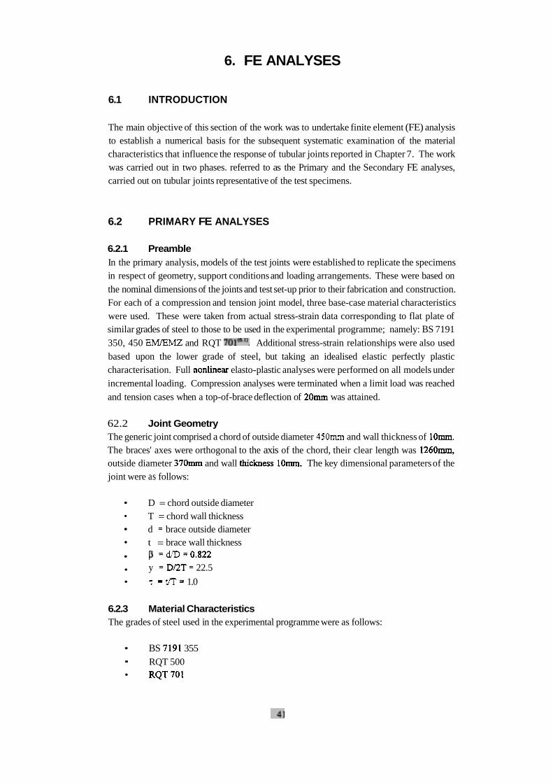
Figure 5.3 shows a frequency histogram of values for DT joints under compression andtension in the screened database. The histogram has been subdivided into compression andtension specimens, and further into those for which the material yield strength is less than orequal to the HSE limit of 0.7 times the material ultimate strength and those for which it is
greater. It should be noted on this histogram that the value listed on the X axis is that of theupper end of the range, ie. 0.5 denotes the range 0.4 0.5. It can be seen that the
distribution is fairly irregular with the mode beta value in the range and largestvolumes of ratios clustered within the ranges and 1.0. The UEG guide

gives typical values for this from a survey of offshore platforms.
It should also be noted that the only tension joint results within the range are from this study.
5.4.2 Experimental Joint StrengthStrengths of the DT compression and tension joints from the screened database have beenplotted against in Figure 5.4. The results of the current programme of tests are indicated byopen symbols. The strengths have first been normalised in two alternative ways by dividingthe measured experimental joint strength by the HSE mean strength formula based on:
the measured material yield strength
the lesser of the actual material yield strength and 0.7 times the actual materialultimate strength (ie. the HSE restriction of material yield strength).
As can be seen if measured material yield strength is used, the spread of normalised strengths
for compression joints is confined mainly to a band bounded principally by about 0.9 and 1.2at the lower and upper extremes respectively. The exceptions to this appear to be three joints
having normalised between 1.3 and 1.4 with valuesa little less than 0.5 and the twotest results from this study having normalised strengths of 0.73 and 0.8 These are the results
for and respectively.
As regards tension joints using the same normalisation, the spread of normalised strengthsappears much wider than for the compression joints. Although the spread for a value of 1.0
is similar to that for the lower values of the tendency seems to be for the normalised strengths to all lie at values greater than unity at = .O. It is worth noting that the tension
joint results generated by the current programme all lie within the spread of the previous test
results.
The statistics associated with the joint strengths normalised with respect to measured material
yield strength are as follows:
Mean Standard COVdeviation
Compression 1.055 0.114 10.8Tension 1.151 0.349 30.3
and these indicate the greater variability in the tension results as compared with thecompression ones. This is probably due to the differing types of failure mechanism in thecases of the tension specimens: brittle fracture and tearing.
The effect of derating the material yield strength in relation to the use of the HSE mean joint strength formula can be observed. It should be recalled that the great majority of the joints hadmaterial yield in excess of the HSE limiting value of 0.7 times the ultimate strength(68 out of 74 for compression and 24 out of 27 for tension).
The general effect of applying the material yield derating is to increase the normalised
joint strengths of the majority of the specimens relative to unity, thereby rendering the HSE

mean strength formula safer as a predictor. This is particularly the case for the compressionspecimens where the unity line becomes almost a lower bound. However, since some specimens would have their normalised strengths unaltered by derating the material yield
strength (i.e. those with 0.7) an additional effect of applying the 0.7 factor to the other
joints is to increase the spread of the normalised strengths.
These factors are reflected in the statistics associated with this normalisation, which are as
follows:
Mean Standard COVdeviation
Compression 1.192 0.151 12.6Tension 1.301 0.371 28.5
Figure 5.4 also confirms that including 0.7 in the HSE equation underpredicts the capacity on
the whole as evidenced by the test data.

Tabl
e5.
1
Dis
trib
utio
nof
mat
eria
lyie
ldst
ren
gth
s b
etw
een
join
t and
load
type
s fo
r th
eun
scre
ened
dat
abas
e (s
cree
ned
DT
inb
race
s

Unscreeneddatabase
200strength
new data
A data
A data
Figure 5.1Scatter plots of material yield to ultimate strength ratio versus
yield and ultimate strength
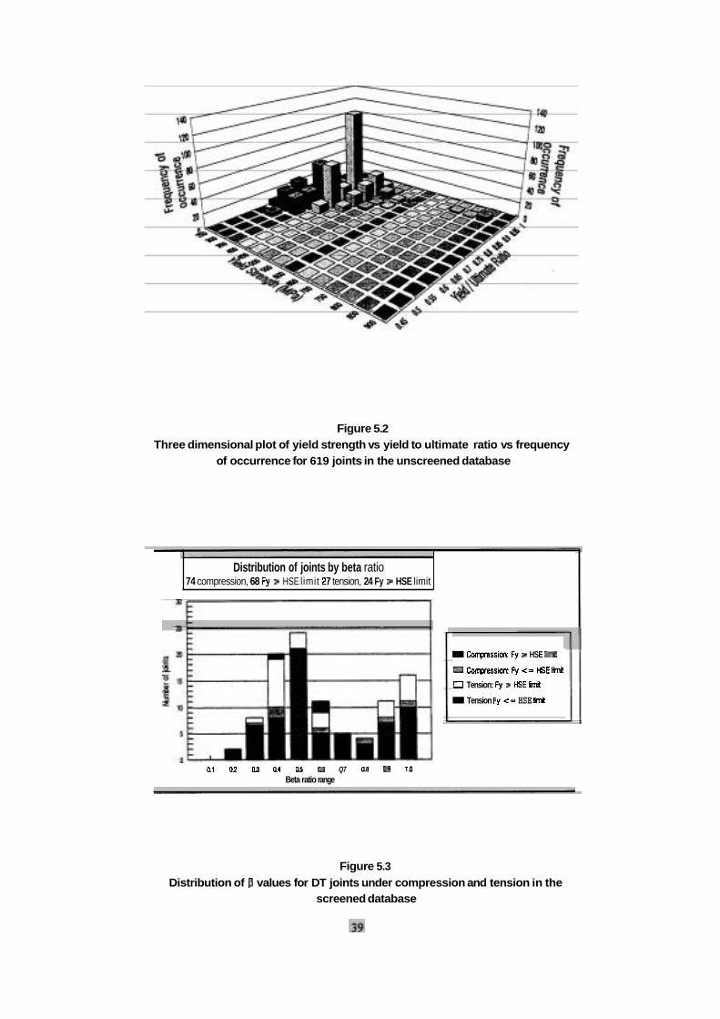
Figure 5.2Three dimensional plot of yield strength vs yield to ultimate ratio vs frequency
of occurrence for 619 joints in the unscreened database
Distribution of joints by beta ratio74 compression, 68 HSE limit tension, 24 Fy HSE limit
Q7Beta ratio range
I HSE
Tension:
ITension HSE
Figure 5.3
Distribution of values for DT joints under compression and tension in thescreened database

in ofda
ta74
020
30.4
050
609
DTjo
ints
Inte
nsio
nDT
join
tsin
tens
ion
Fig
ure
5.4
DT
join
tsu
nd
er c
om
pre
ssio
n a
nd
ten
sio
n: e
xper
imen
tal j
oint
stre
ng
th n
orm
alis
ed w
ithre
spec
tto
the
HS
Em
ean
str
eng
th fo
rmul
a
6. FE ANALYSES
6.1 INTRODUCTION
The main objective of this section of the work was to undertake finite element (FE) analysisto establish a numerical basis for the subsequent systematic examination of the material characteristics that influence the response of tubular joints reported in Chapter 7. The workwas carried out in two phases. referred to as the Primary and the Secondary FE analyses,carried out on tubular joints representative of the test specimens.
6.2 PRIMARY FE ANALYSES
6.2.1 PreambleIn the primary analysis, models of the test joints were established to replicate the specimensin respect of geometry, support conditions and loading arrangements. These were based onthe nominal dimensions of the joints and test set-up prior to their fabrication and construction.For each of a compression and tension joint model, three base-case material characteristics were used. These were taken from actual stress-strain data corresponding to flat plate ofsimilar grades of steel to those to be used in the experimental programme; namely: BS 7191350, 450 and RQT Additional stress-strain relationships were also usedbased upon the lower grade of steel, but taking an idealised elastic perfectly plastic characterisation. Full elasto-plastic analyses were performed on all models underincremental loading. Compression analyses were terminated when a limit load was reachedand tension cases when a top-of-brace deflection of was attained.
62.2 Joint GeometryThe generic joint comprised a chord of outside diameter and wall thickness of The braces' axes were orthogonal to the axis of the chord, their clear length was outside diameter and wall The key dimensional parameters of thejoint were as follows:
D = chord outside diameterT = chord wall thickness d brace outside diameter t = brace wall thickness
y 22.5
1.0
6.2.3 Material CharacteristicsThe grades of steel used in the experimental programme were as follows:
BS 355RQT 500
Prior to the performance of the material tests reported in Section 3, British Steel supplied typical engineering stress-strain relationships for the first and last of these materials tensiletests over a range of strains which included strain hardening. Similar data were supplied for a 450 steel. The key mechanical properties of the materials were as set out in Table6.l and are all expressed in engineering and true terms.
Table 6.1Key mechanical properties of the three grades of steel used in the Primary FE
analysis. Engineering values. True values in brackets
SteelGrade
355
450
700
Young's
Modulus
E
Ultimate
Strength
Yield
Ultimate
Ratio
Yield Strain atStrain Strain
Hardening
0.21 4.49(0.21) (4.60)
Ultimate
Strain
29.2(25.7)
17.6,
16.0
The following points are worth noting:
The yield to ultimate ratio of the 355 grade steel would lie at the upper end of the spread of the results in the test database (see Chapter and the ratios for the other of steel are consistent with the trends shown in the database analysis. In terms of yield to ultimate ratio, all three steel grades significantly exceed the HSE design limit of 0.7.
All steel grades exhibit linear elasticity followed by a yield plateau, followed bystrain hardening to ultimate stress. The length, in terms of strain, of the yield plateaushortens as the grade of steel increases; for example, the length corresponding withthe 700 grade steel is about half of that for the 355 grade. A similar effect can beobserved for the magnitude of the ultimate strain.
62.4 Finite Element Model The axially loaded DT joint has three planes of symmetry and, therefore, for the preliminary analyses a model that represents only one eighth of the joint was built.
The model was based around the median surface dimensions of the joint. Eight-noded thickshell elements with four Gauss points were used type Themesh, and sizes and types of element were based on extensive previous experience in modellingof joints, and work reported by Delft University of Modelling of the weldedconnection between braces and chords was not undertaken. The connection details at the endsof the braces were modelled as stiff diaphragmend plates using thick elements, the same as for the joint, and these were used as the medium to apply the axial loading in the brace. The chord ends were left open.
The boundary conditions applied to the model stem principally the symmetry of the joint.The only displacement at the centre of the end of the brace that was permitted was parallel tothe load, ie. a translation normal to its plane. All others were suppressed at the point of loadapplication.
Loading and Analysis CasesThe loading on the finite element model was a single concentrated force at the centre of the brace end plate, the line of action of which was collinear with the brace axis. This load was directed either away or towards the chord to achieve the tensile and compressive load cases, respectively. In order to achieve convergence to equilibrium displacementscorresponding with a given load on a nonlinear response curve, use was made of theSolution algorithm. This enabled the response through and beyond limit points to bedetermined.
A total of eight analysis cases were performed derived from the following:
A compression and a tension loading case for each of the three grades of steel using the actual behaviour of the material, i.e. including the effect of material
strain hardening.
A compression and a tension loading case for the 355 grade of steel using anperfectly plastic material.
6.2.6 Results and DiscussionWith reference to Figure 6.1, the compression loaded joint exhibited a limit point response for all steel grades wherein the loaddeformation curve exhibits a peak load, which represents the capacity of the joint. For the joint correspondingwith the 355 grade of steel there appeared tobe very little difference between behaviour pertaining to the two alternative materialcharacteristics (incorporating strain hardening and elastic-perfectly plastic).
For the tension loaded joints (Figure regardless of steel grade the joint. exhibited arising response. It should be emphasised that it is not possible
to discern the capacity of the joint these because no limit load is observed and, therefore, strength may be limited by the attainment of critical strain and cracking. For the joint with the355 grade of steel and the two alternative material characterisations, as was the case with thecompression joint, very little difference between the two responses is evident.
6.2.7 Findings from Primary FE AnalysesTable 6.2 presents ultimate deflections and loads for the DT joints in compression for the threegrades of steel the FE analysis. The results for the 355 correspond with thestrain characteristic incorporating strain hardening. Tabulated along with these are thepredictions of capacity resulting the use of the HSE mean inconjunction with the actual material yield strength, and times the material ultimate strength.With reference to Table 6.1 all three grades of material have yield strength to ultimate strength ratios in excess of the HSE limiting value and would, in terms of current design practice, have their capacity derated to the lower value. Also given in Table 6.2 is a column headed "Impliedfactor on F, for FE". This tabulates the multiplying factor on material ultimate thatmust be used in the HSE mean joint strength formula so that the latter gives precisely the FE result.

Table6.2DT joints in compression :ultimate deformation and loads from primary FE analysis
and HSE mean ultimate loads based on actual material yield strength and 0.7 times material ultimate strength
As can be seen fiom Table 6.2 for all three grades of material the capacity fiom the FE analysislies between the two values obtained from the use of the HSE mean strength formula. In thecase of the 355 grade, the FE result lies closest to the HSE mean value correspondingwith the actual material yield For the 500 and 700 grades of steel, however, the FE results lievery close to the median of the two HSE mean strength predictions. It is notable for all three grades of steel that the implied factor on F, for the FE results lies close to
Steelgrade
355
500
700
As has been observed earlier, the tension loaded joints do not exhibit a peak load in terms ofloaddisplacement response and, in practice, failure occurs by the propagationof cracks around the weld toe. There is no established method used to model this type of response using finiteelement techniques, and the mechanisms of crack initiation are the subject of fundamentalresearch. Notwithstanding this, a possible method of joint failure fiom the FEanalysis is to monitor the strains in the saddle location of the joint and compare them with material ultimate strains.
Examination of the strains for the tension joint with the 700 grade of material revealed peak strains of the order of 14.8%(fiom Table 6.1 the ultimate strain is 14.0%)at a load of 1828 W.This load corresponds very closely with the mean HSE computed load of 1857 obtainedusing the derated material strength. In contrast, however, the tension joint with the 355 gradeof material gave peak strains of 14.6% and 20.5% at loads of 1076 and 1544respectively. These are to be compared with an ultimate strain of 25.7% (Table andpossible HSE mean loads of 1098 and 1327 W. The situation in the case of this materialis much less conclusive. Strain is influenced by local physical constraint in the case of actual joints, and by the mesh size used in finite element models.
6.3 SECONDARY FE ANALYSES
Ultimate from FE analysis
6.3.1 PreambleThis sub-section describes the work pertaining to the Secondary FE analyses. The objective was to construct FE models validated against the experiments. Material properties from the tensile coupon tests described in Chapter 3 and geometric properties fiom the measurements
Deformation
a
15
18
33
Impliedfactor onF, for FE
0.81
0.78
0.80
Load
b
720
853
1200
Mean ultimate load fromHSE based on:
Actual F,
C
748
952
1422
d
619
767
1047
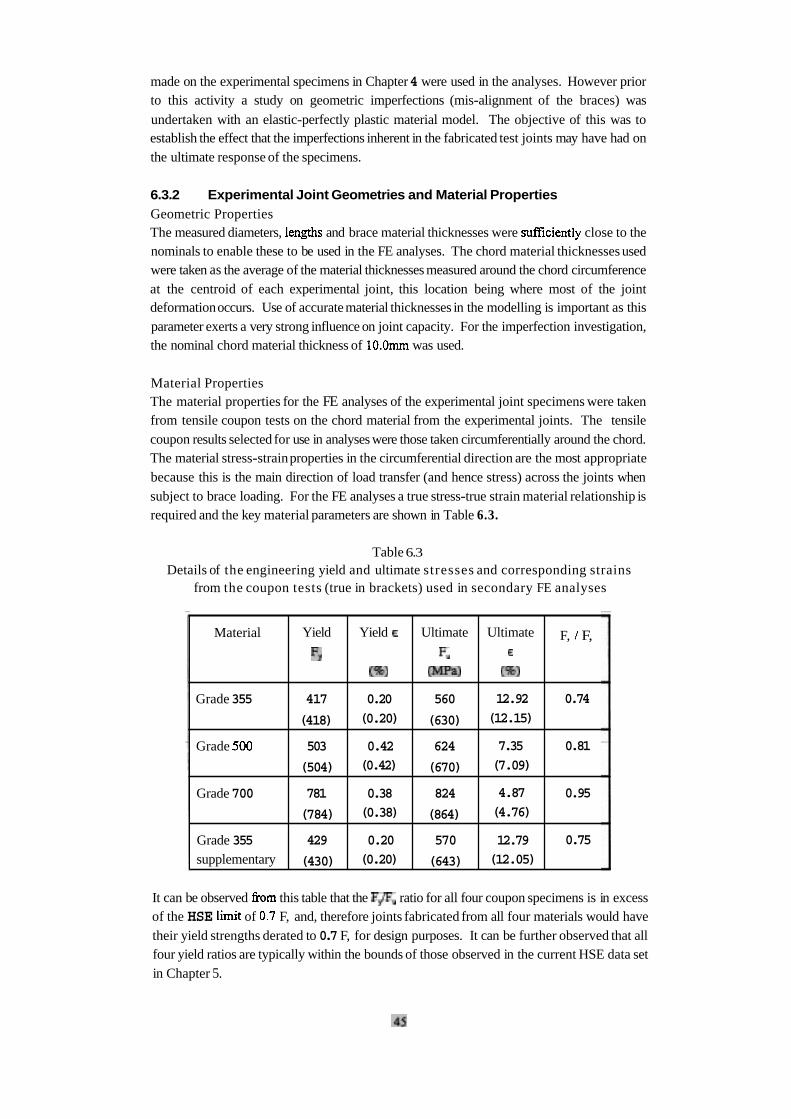
made on the experimental specimens in Chapter4were used in the analyses. However prior to this activity a study on geometric imperfections (mis-alignment of the braces) was
undertaken with an elastic-perfectly plastic material model. The objective of this was toestablish the effect that the imperfections inherent in the fabricated test joints may have had onthe ultimate response of the specimens.
6.3.2 Experimental Joint Geometries and Material Properties Geometric PropertiesThe measured diameters, and brace material thicknesses were close to thenominals to enable these to be used in the FE analyses. The chord material thicknesses usedwere taken as the average of the material thicknesses measured around the chord circumference at the centroid of each experimental joint, this location being where most of the jointdeformationoccurs. Use of accurate material thicknesses in the modelling is important as thisparameter exerts a very strong influence on joint capacity. For the imperfection investigation, the nominal chord material thickness of was used.
Material PropertiesThe material properties for the FE analyses of the experimental joint specimens were takenfrom tensile coupon tests on the chord material from the experimental joints. The tensilecoupon results selected for use in analyses were those taken circumferentially around the chord.The material stress-strainproperties in the circumferential direction are the most appropriatebecause this is the main direction of load transfer (and hence stress) across the joints whensubject to brace loading. For the FE analyses a true stress-true strain material relationship isrequired and the key material parameters are shown in Table 6.3.
Table 6.3Details of the engineering yield and ultimate stresses and corresponding strains
from the coupon tests (true in brackets) used in secondary FE analyses
It can be observed this table that the ratio for all four coupon specimens is in excessof the HSE of F, and, therefore joints fabricated from all four materials would havetheir yield strengths derated to0.7F, for design purposes. It can be further observed that all four yield ratios are typically within the bounds of those observed in the current HSE data setin Chapter 5.
F, F,
0.74
0.81
0.95
0.75
Material
Grade355
Grade
Grade700
Grade 355supplementary
Yield
417
(418)
503
(504)
781
(784)
429
(430)
Yield
0.20(0.20)
0.42(0.42)
0.38(0.38)
0.20(0.20)
Ultimate
560
(630)
624
(670)
824
(864)
570
(643)
Ultimate
12.92(12.15)
7.35(7.09)
4.87(4.76)
12.79(12.05)
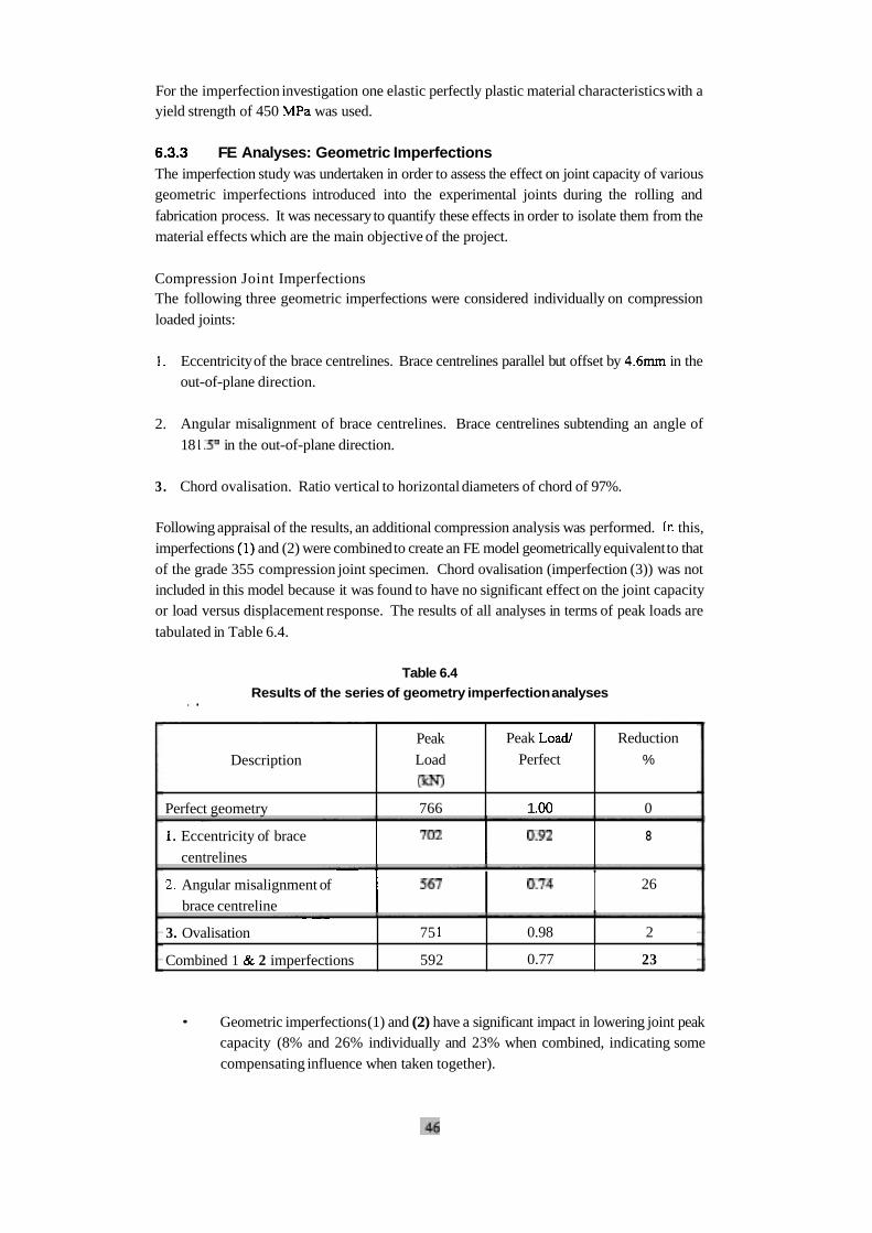
For the imperfection investigation one elastic perfectly plastic material characteristicswith ayield strength of 450 was used.
FE Analyses: Geometric Imperfections The imperfection study was undertaken in order to assess the effect on joint capacity of variousgeometric imperfections introduced into the experimental joints during the rolling and
fabrication process. It was necessary to quantify these effects in order to isolate them from the material effects which are the main objective of the project.
Compression Joint ImperfectionsThe following three geometric imperfections were considered individually on compression loaded joints:
Eccentricityof the brace centrelines. Brace centrelines parallel but offset by in theout-of-plane direction.
2. Angular misalignment of brace centrelines. Brace centrelines subtending an angle of 18 in the out-of-plane direction.
3. Chord ovalisation. Ratio vertical to horizontal diameters of chord of 97%.
Following appraisal of the results, an additional compression analysis was performed. this,imperfections and (2) were combinedto create an FE model geometrically equivalentto thatof the grade 355 compression joint specimen. Chord ovalisation (imperfection (3)) was notincluded in this model because it was found to have no significant effect on the joint capacity or load versus displacement response. The results of all analyses in terms of peak loads are
tabulated in Table 6.4.
Table 6.4
Results of the series of geometry imperfection analyses. .
P-
Eccentricity of brace 8
centrelines
Description
Perfect geometry
Angular misalignment of I I 26
brace centreline
Peak
Load
766
3. Ovalisation
Geometric imperfections (1) and (2) have a significant impact in lowering joint peakcapacity (8% and 26% individually and 23% when combined, indicating somecompensating influence when taken together).
Peak
Perfect
1
Combined 1 2 imperfections
Reduction
%
0
75
592
0.98 2
0.77 23
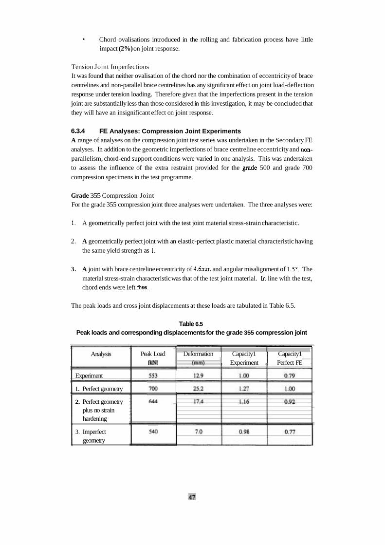
Chord ovalisations introduced in the rolling and fabrication process have littleimpact (2%)on joint response.
Tension Joint ImperfectionsIt was found that neither ovalisation of the chord nor the combination of eccentricityof brace
centrelines and non-parallel brace centrelines has any significant effect on joint load-deflectionresponse under tension loading. Therefore given that the imperfections present in the tension
joint are substantiallyless than those considered in this investigation, it may be concluded thatthey will have an insignificant effect on joint response.
6.3.4 FE Analyses: Compression Joint Experiments A range of analyses on the compression joint test series was undertaken in the Secondary FEanalyses. In addition to the geometric imperfections of brace centreline eccentricity and
parallelism, chord-end support conditions were varied in one analysis. This was undertakento assess the influence of the extra restraint provided for the 500 and grade 700
compression specimens in the test programme.
Grade 355 Compression JointFor the grade 355 compression joint three analyses were undertaken. The three analyses were:
A geometrically perfect joint with the test joint material stress-strain characteristic.
2. A geometrically perfect joint with an elastic-perfect plastic material characteristic having
the same yield strength as
3. A joint with brace centrelineeccentricity of and angular misalignment of 1 The
material stress-strain characteristicwas that of the test joint material. line with the test,chord ends were left
The peak loads and cross joint displacements at these loads are tabulated in Table 6.5.
Table 6.5Peak loads and corresponding displacements for the grade 355 compression joint
Analysis
Experiment
Perfect geometry
2. Perfect geometryplus no strainhardening
3. Imperfectgeometry
Peak Load Deformation Capacity1 Capacity1 Experiment Perfect FE
The following observations can be made:
Neglect of strain hardening in the perfect joint reduced the capacity by 8%.
Both perfect joint models had peak loads significantly greater than the initial peak load in the test specimen (27%and 16%).
When the geometric imperfections in the test specimen are accounted for the peakload is in very close agreement with that of the test specimen.
The geometric imperfections in this analysis case cause a decrease of 23% in peakload from the corresponding perfect joint peak load.
Grade 500 Compression JointFor the Grade 500 compression joint a total of five analyses was undertaken. These were as
follows:
A geometrically perfect joint.
A joint with brace centreline eccentricity of and angular misalignment of 0.75".The chord ends were unrestrained.
A joint identical to 2, above, with the chord ends prevented from lateral displacement and rotation. The chord end boundary conditionsclosely replicated those present in the test on this specimen.
A joint similar to 3, above, with the brace loading point free to deflect out of the jointplane, other boundary conditions remaining identical. This was undertaken to assess the
potential extreme effect of lateral deflection at the end plate of the loading (jack) arrangement during the test.
A joint with boundary conditions at the load point between those of the two extremes incases 3 and 4. A spring support was provided in the out-of-plane direction with a nominalstiffness of 139 The correct stiffness is impossible to determine and the lateral deflection response of the arrangement is likely to be nonlinear. Nevertheless this
approximation of the lateral 'sway' response provides a useful insight into the potentialdiscrepancy between the experimental and the capacities.
The peak loads and cross joint displacements at these loads are tabulated in Table 6.6 and thefollowing observations can be made:
The perfect joint sustains a greater load than the test specimen in the range ofdeformation values around its peak load - (818 versus 717).When the geometric imperfections in the test specimen are accounted for in case 2,peak capacity is lowered from 818 to However, when the chord ends are restrained from twisting and lateral (out-of-jointplane) displacement (case 3)this lowering of the capacity from the geometrically perfect joint case does notoccur.

Table 6.6
Peak loads and corresponding displacements for the grade 500 compression joint
3. Imperfect geometryrestraint I
Analysis
Experiment
1. Perfect geometry
2. Imperfect geometry No chord restraint
Peak Load
818
652
Deformation
4. Imperfect geometry No load point restraint
5. Imperfect geometrySpring load point
restraint
* Load at an equivalent displacement to FE analyses (not a peak)
612
680
Capacity I Capacity I
Maintaining the chord end restraints but, allowing the load point to deflect out of
the joint plane (case 4) reduces peak capacity by 25%.
Stiffening the side sway of the load point increases capacity over the 'free to sway'
lower bound case. The response can be seen to fall reasonably close to that of the
comparable experimental result.
It was found that the deformed shape plot of the spring case very closely replicated the
behaviour in the experimental test on this joint. It can be concluded that the response
of this joint could have been influenced by a combination of the geometric imperfections and
the lateral flexibility of the load support arrangement at the top of the brace, or the supporting
arrangements at the chord ends.
Grade 700 Compression JointFor the grade 700 compression joint two analyses were undertaken:
1. A geometrically perfect joint.
2. A joint with brace eccentricities and angular misalignment equal to those measured prior
to the test on the grade 355 compression specimen.
The peak loads and cross joint displacements at these loads are tabulated in Table 6.7.
Table 6.7Peak loads and corresponding displacements for the grade 700 compression joint
The following observations can be made:
Analysis
Experiment
1. Perfect geometry
2. Imperfect geometry
The perfect joint model had a peak load significantly greater than the initial peakload in the test specimen (1256 versus 1064).
The joint with the imperfections experiences a fall of 30% in peak capacity whencompared to the perfect joint. This compares with a corresponding fall of 23% for
the same imperfections in the grade 355 FE analyses. Therefore as the yield stressof the material increases, the effect of the geometric imperfections on lowering joint
strength increases.
Peak Load
1064
1256
882
Supplementary Grade 355 Compression JointFor the supplementary grade 355 compression joint one analysis was undertaken on a
nominally perfect joint. The analysis used the test joint material stress-swain relationship. Theresults are given in Section 6.3.6, below.
6.3.5 FE Analyses: Tension Joint ExperimentsA set of analyses on the tension joint test series was undertaken in the Secondary FE analyses.Geometric imperfections were not considered as the effect of these was found to be negligible.Observation of the imperfections present in the tension joint specimens (see Table 4.1) alsoreveals that the magnitudes are significantly less than those considered in sub-sectionwhere little effect was observed, further supporting the conclusion that the effects will benegligible. Important joint loads for the three material grades are summarised in Table 6.8.
Deformation
16.5
36.0
8.1
Table 6.8Summary of loads for DT tension joints: peak (final) loads from tests, cracking loads
and HSE mean ultimate loads based on actual material yield strength
Capacity1Experiment
1.00
1.18
0.83
Mean Ultimate Load
From HSE Based On:
Actual F,
CapacityPerfect FE
0.85
1
0.70
Joint ID
Experimental Load atwhich
Detected
(Table 4.3)
900
800
800
Peak (Final) LoadFrom Experiment
(Table 4.2)
1454
1604
1868

Grade 355 Tension JointFor the grade 355 tension joint two analyses were performed using the measured materialstress-strain characteristic. These two analyses were:
A geometrically perfect joint.
2. A modified model with an approximate weld profile included.
The peak (final) load in the test specimen was 1454 and the capacity calculated accordingto the HSE mean formulation (based on the yield stress) was 1163 Test reports from the laboratory indicate that at a load of 900 a crack of length had formed around the toe
of one brace saddle location.
It was found from the analyses that:
The inclusion of an approximate weld profile stiffened the response when comparedto the perfect joint case, but there remained a discrepancy between the test and FEresults.
The response of the specimen with this basic weld profile included began to deviate
from the test at a load of around 500 It was noted earlier that at 900 a crack
of length was present at one brace saddle location. In the test the crack willhave developed at a lower load and propagated as the load increased to 900
This crack development would cause the test response to become less stiff than that of the FE.
The ability to model the weld and the crack initiation process is important if tensile
responses are to be tracked accurately, but is beyond the capabilities of generalpurpose finite element packages. The accurate prediction of nonlinear tensile
structural responses therefore remains unresolved.
Grade 500 Tension JointFor the 500 tension joint an analysis was performed using the test joint material
strain characteristic. The peak (final) load observed in the test specimen was 1604 and thecapacity calculated according to the HSE mean (based on the yield stress) is 1437 Testreports from the laboratory indicate that at a load of 800 cracks of length or more had formed at all four saddle locations in the chord.
It was observed that the FE loaddeflection results are in good agreement with the test results
up to a load of around 600 The deviation in response which occurs after this load level
(as the responseof the test joint becomes less stiff) is explained by the formation of cracks inthe test joint which are not accounted for in the FE analysis.
Grade 700 Tension JointFor the grade 700 tension joint an analysis was performed using the test joint material stress-strain characteristic. The peak (final) load observed in the test was 1868 and the capacity
calculated according to the HSE mean (based on the yield stress) is 2573 Test reports
from the laboratory indicate that at a load of 800 two cracks of lengths and
had formed at two of the saddle locations.
It was observed that the FE results, given the lack of weld modelling, are in reasonableagreement with the experiment up to a load level around 1000 The deviation in responsebetween the two sets of results beyond this load level is again attributed to the cracking in the
test specimen which is not replicated in the FE model.
6.3.6 Findings from FE Secondary Analyses Compression JointsFor the compression joints it was found that brace centreline angular misalignment and brace centreline eccentricity can have a significant effect on joint response. For the purposes of thissection the compression joint FE analyses performed on joints with no imperfections in thegeometry are discussed with respect to the effect of the material properties on the joint response.
Table 6.9 Summary of Secondary FE analyses on DT compression joints: ultimate FE loads
(peak) and HSE mean ultimate loads based on actual material yield strengthand 0.7 times material ultimate strength
Peak load Mean ultimate load from Impliedfrom HSE based on:
experiment , F,, for FE
Table 6.9 presents ultimate loads for the DT joints in compression for the four perfect
geometry FE analyses. Tabulated alongside these are the predictions of capacity resulting
from the use of the HSE mean strength in conjunction with the actual material yield strength, and 0.7 times the material ultimate strength. reference to Table 6.3 all four sets
of material properties have material yield strength to ultimate strength ratios in excess of theHSE limiting value and would, in principle, have their capacity derated to the lower value.
Also given in Table 6.8 in the final column is an "implied factor on F, for FE". This tabulatesthe multiplying factor on material ultimate strength that must be used in the HSE mean joint
strength formula so that the latter gives precisely the FE result.
As can be seen from this table for the three analyses covering the two lower steel grades the
FE ultimate capacities are in close agreement with the HSE mean ultimate capacities calculated
according to the yield stress value. For the analysis on the 700 grade joint the FE result lies

close to the median of the twoHSEmean strength predictions. It is notable that for all three
grades (four analyses) of steel that the implied factor on F, for the FE results lies close to 0.8.This finding is closely in line with that in the primary analyses in sub-section 6.2
Tension JointsFor the tension joints it was found that geometric imperfections of all the types considered
have very little effect on joint response.
In terms of the analyses undertaken on the tension joint specimens, meaningful comparison
with the tests at ultimate load is extremely difficult. There are two reason for this. the
FE model is unable to predict crack formation in the material and therefore the effect that this
would have on joint response. The formation of cracks in tension test specimens is the main
mode of failure. Secondly, attempts to determine the loads at which cracks would form in the
FE analysis by examining plastic strain levels and comparing these with rupture strains from
the tensile coupon test were of limited success. This was due in part to the fact that the initial
state of stress in the FE model (prior to loading) was zero and hence not compatible with that
of the tests where significant residual stresses would be present due to the rolling and welding
processes.
Attempts to compare the FE with the HSE mean and the test results using a deformation limit
were largely unsuccessful. Table 6.10 summarises the results from the deformation
limit calculations using the experimental and finite element results.
Table 6.10Experimental tension DT joints: loads corresponding to deformation limits
* based on 2 brace length + chord diameter
JointLoad from
finite element
results
Notwithstanding this, reasonable agreement between the experimental and finite element
results were obtained for load-deflection regimes of response prior to cracking in the tests.
This provided further that the finite element models were well-calibrated against
the test results.
Material F,
417
503
781
Deformation
limit*
12
15
23
Load from
experimental
results
530
760
1200
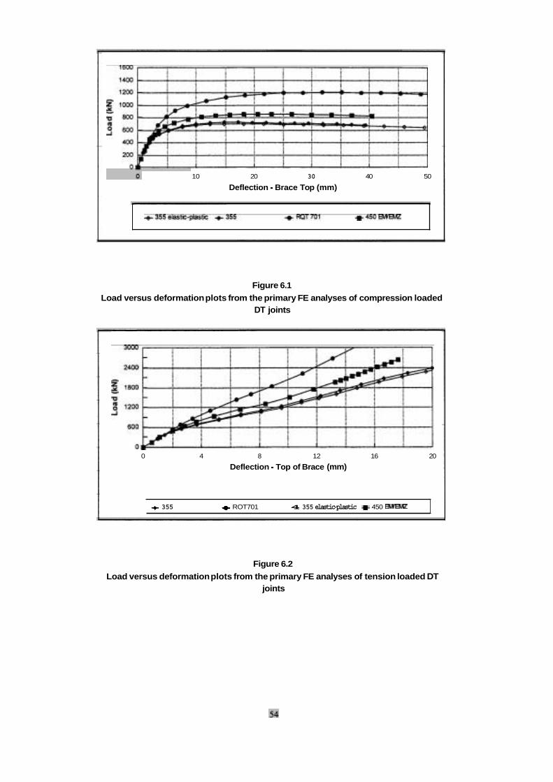
10 20 30 40 50
Deflection Brace Top (mm)
Figure 6.1
Load versus deformationplots from the primary FE analyses of compression loadedDT joints
0 4 8 12 16 20
Deflection Top of Brace (mm)
355 ROT701 4355elastic-plastic 450 I
Figure 6.2
Load versus deformation plots from the primary FE analyses of tension loaded DTjoints
7.1 INTRODUCTION
This Chapter reports on Activity 6 of the study, and is concerned with the development ofinitial recommendations for revising the design guidance for DT tubular joints. This is withparticular regard to the characteristics (notably high yield to ultimate strength ratios) peculiarto high strength steels. The developments have been made by supplementing the workreported in the preceding chapters with further static strength database analyses and finiteelement calculations.
7.2 FURTHER ANALYSIS OF DT JOINTS SCREENED DATABASE
7.2.1 Material Strength Formulations and Database ManipulationIn further manipulation of the DT joints subset of the screened static strength database, theHSE mean strength formulae were used and ways of introducing the material strength were considered. Thus, it was assumed that the portionsof the formulae that refer to geometricaspects would remain the same in any new formulations proposed. Three material
representations were tried, namely: a yield ratio limit, a flow stress limit and a constant factoron yield ratio, as set out below.
In the case of the yield ratio limit the formulation is:
where F, = material yield strength to be used in the HSE mean joint strength formula
F, = actual material yield strength
F, actual material ultimate strength K yield ratio limit.
The reasons for the choice of this particular formulation are: first, that it follows current design practice; and, second, that indications previous Activities in the project were that its useis likely to produce a reasonable approach. K is set to 0.7 in the HSE Guidance and a valueof unity would result in the use of the actual material yield strength in joint strengthcalculations, regardless of the value of the ultimate tensile strength.
For the flow stress approach the formulation taken is:
F, = F, + R( F" - F,)
where R = flow stress limit
and the other symbols have been defined previously.
The flow stress limit is an obvious one to investigate, particularly for tension loaded cases.This type of approach is used in a variety of other areas, for example, in the strength ofpipelines.
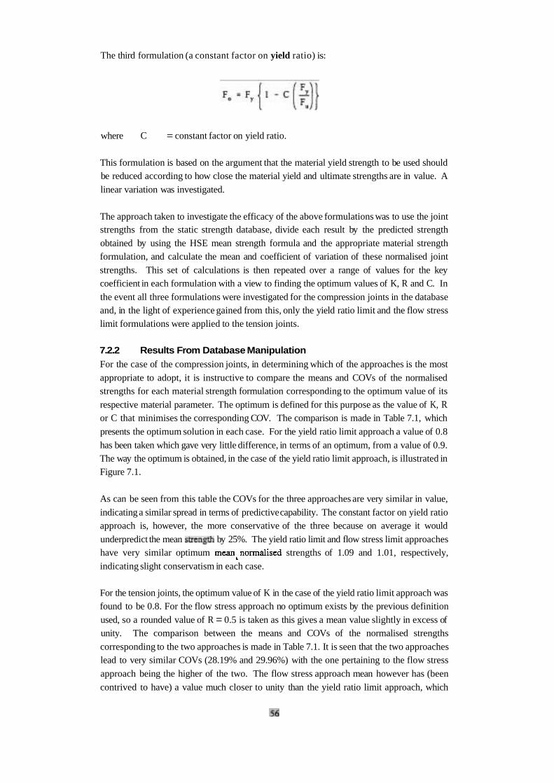
The third formulation (a constant factor on yield ratio) is:
where C = constant factor on yield ratio.
This formulation is based on the argument that the material yield strength to be used shouldbe reduced according to how close the material yield and ultimate strengths are in value. A
linear variation was investigated.
The approach taken to investigate the efficacy of the above formulations was to use the jointstrengths from the static strength database, divide each result by the predicted strength
obtained by using the HSE mean strength formula and the appropriate material strengthformulation, and calculate the mean and coefficient of variation of these normalised joint
strengths. This set of calculations is then repeated over a range of values for the keycoefficient in each formulation with a view to finding the optimum values of K, R and C. In
the event all three formulations were investigated for the compression joints in the database and, in the light of experience gained from this, only the yield ratio limit and the flow stresslimit formulations were applied to the tension joints.
7.2.2 Results From Database Manipulation For the case of the compression joints, in determining which of the approaches is the most
appropriate to adopt, it is instructive to compare the means and COVs of the normalised strengths for each material strength formulation corresponding to the optimum value of its
respective material parameter. The optimum is defined for this purpose as the value of K, Ror C that minimises the corresponding COV. The comparison is made in Table 7.1, which
presents the optimum solution in each case. For the yield ratio limit approach a value of 0.8
has been taken which gave very little difference, in terms of an optimum, from a value of 0.9.The way the optimum is obtained, in the case of the yield ratio limit approach, is illustrated inFigure 7.1.
As can be seen from this table the COVs for the three approaches are very similar in value,
indicating a similar spread in terms of predictivecapability. The constant factor on yield ratioapproach is, however, the more conservative of the three because on average it would
underpredict the mean by 25%. The yield ratio limit and flow stress limit approacheshave very similar optimum strengths of 1.09 and 1.01, respectively,
indicating slight conservatism in each case.
For the tension joints, the optimum value of K in the case of the yield ratio limit approach wasfound to be 0.8. For the flow stress approach no optimum exists by the previous definition
used, so a rounded value of R = 0.5 is taken as this gives a mean value slightly in excess ofunity. The comparison between the means and COVs of the normalised strengths
corresponding to the two approaches is made in Table 7.1. It is seen that the two approacheslead to very similar COVs (28.19% and 29.96%) with the one pertaining to the flow stress
approach being the higher of the two. The flow stress approach mean however has (been
contrived to have) a value much closer to unity than the yield ratio limit approach, which
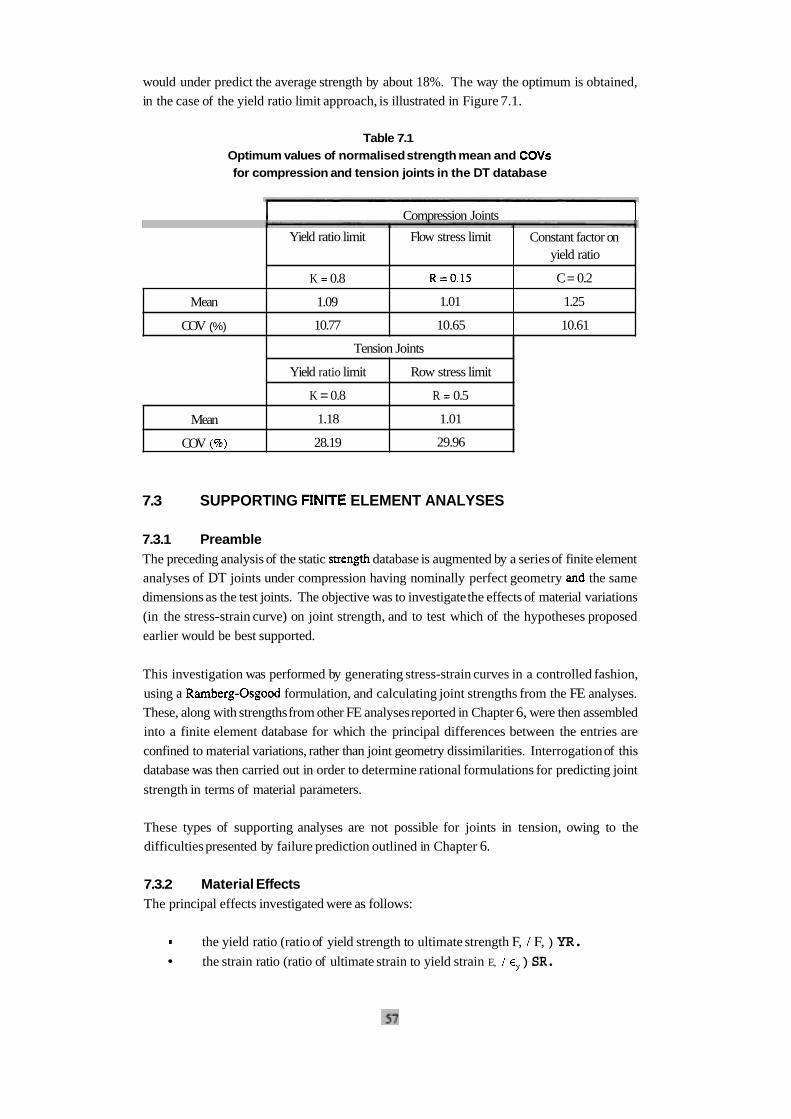
would under predict the average strength by about 18%. The way the optimum is obtained,
in the case of the yield ratio limit approach, is illustrated in Figure 7.1.
Table 7.1Optimum values of normalised strength mean and for compression and tension joints in the DT database
Compression Joints
Mean
COV (%)
7.3 SUPPORTING ELEMENT ANALYSES
Mean
COV
7.3.1 PreambleThe preceding analysis of the static database is augmented by a series of finite element
analyses of DT joints under compression having nominally perfect geometry the same
dimensions as the test joints. The objective was to investigate the effects of material variations
(in the stress-strain curve) on joint strength, and to test which of the hypotheses proposed
earlier would be best supported.
Yield ratio limit
K 0.8
1.09
10.77
This investigation was performed by generating stress-strain curves in a controlled fashion,
using a formulation, and calculating joint strengths from the FE analyses.
These, along with strengths from other FE analyses reported in Chapter 6, were then assembled
into a finite element database for which the principal differences between the entries are
confined to material variations, rather than joint geometry dissimilarities. Interrogationof this
database was then carried out in order to determine rational formulations for predicting joint
strength in terms of material parameters.
Tension Joints
These types of supporting analyses are not possible for joints in tension, owing to the
difficulties presented by failure prediction outlined in Chapter 6.
Flow stress limit
1.01
10.65
Yield ratio limit
K = 0.8
1.18
28.19
7.3.2 Material EffectsThe principal effects investigated were as follows:
Constant factor onyield ratio
C= 0.2
1.25
10.61
Row stress limit
R 0.5
1.01
29.96
the yield ratio (ratio of yield strength to ultimate strength F, F, ) YR.the strain ratio (ratio of ultimate strain to yield strain E, ) SR.
A total of material stress-strain curves were generated arising from a combination of
three material yield strengths of 500,600 and 700
three yield ratios of andthree strain ratios.
one elastic-perfectly plastic response for each steel yield strength.
Thus for each material yield strength taken, ten material characteristics were used: onecorresponded with an elastic-perfectly plastic stress-strain curve, whilst the remaining nine
arose from the combinations of different yield and strain ratios. It was judged important thatthese nine characteristics were generated in a systematic and coherent manner and so aprocedure involving a Ramberg-Osgood representation was evolved to achieve this.
7.3.3 Finite Element AnalysisAll the thirty stress-straincharacterisationswere converted to true stress-strain and processed
into suitable for use with the finite element package ABAQUS. Each was then used inthe analysisof a geometrically perfect DT joint, under compressive loading, with the following
dimensions:
brace diameter d 360.0mmbrace thickness t 10.0mmchord diameter D 449.5 mm
chord thickness T =
these are similar to the dimensions of the355 grade joint discussed in Chapter 6 of this report.
The most striking characteristic from the load-deflection results from the analyses was that,for a particular material yield strength and yield ratio less than unity (the elastic-perfectly
plastic case), the three curves corresponding to the different strain ratios used were virtually
indistinguishable. This is particularly so at the maximum load, and indicates that the jointstrength is not affected by strain ratio. There is some dependence on yield ratio and, by
comparing results for the different material on yield strength.
These dependencies can be assessed by examiningFigure 7.2 which plots joint strength against yield ratio for fixed values of yield strength, and against yield strength for fixed values of yieldratio. As can be seen the various relationshipsare nearly linear, and whilst there is a slight
sensitivity to yield ratio, the gradients of the joint strength versus yield strength lines are muchsteeper. This linearity would not be so evident in similar plots from, say, the database of joint
test results because of a number of factors including: geometry differences variations,thickness differences and so forth), imperfections, differences in experimental procedure andso on. In addition, the yield ratio would not remain constant as the material yield strengthincreases, but would tend to increase. In the case of Figure 7.2 the only differences betweenthe joints analysed are the yield ratios and material yield strengths. Any dependence of yield
ratio on yield strength would tend to reduce the joint strength from that for a constant yield
ratio, giving a curve for the joint strength versus yield strength relationship, or at least a line with a smaller slope than those of the lines shown in Figure 7.2.
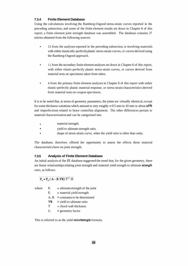
7.3.4 Finite Element Database Using the calculations involving the Ramberg-Osgood stress-strain curves reported in thepreceding subsection, and some of the finite element results set down in Chapter 6 of thisreport, a finite element joint strength database was assembled. The database contains 27entries obtained from the following sources:
12 from the analyses reported in the preceding subsection, ie involving materialswith either elastically-perfectlyplastic stress-strain curves, or curves derived usingthe Ramberg-Osgood approach.
from the secondary finite element analyses set down in Chapter 6 of this report,with either elastic-perfectly plastic stress-strain curves, or curves derived frommaterial tests on specimens taken from tubes.
4 from the primary finite element analyses in Chapter 6 of this report with eitherelastic-perfectly plastic material response, or stress-strain characteristics derivedfrom material tests on coupon specimens.
It is to be noted that, in terms of geometry parameters, the joints are virtually identical, except for some thickness variations which amount to very roughly 0.5 mm in 10 mm or aboutand imperfections related to brace centerline alignment. The other differences pertain tomaterial characterisation and can be categorised into
material strength. . yield to ultimate strength ratio.shape of stress-strain curve, when the yield ratio is other than unity.
The database, therefore, offered the opportunity to assess the effects these material
characteristicshave on joint strength.
7.3.5 Analysis of Finite Element Database An initial analysis of the FE database suggested the trend that, for the given geometry, thereare linear relationships relating joint strength and material yield srength to ultimate
ratio, as follows:
where P, ultimate strength of the joint F, material yield strength
A, B =constants to be determined= yield to ultimate ratio
T chord wall thicknessG = geometry factor
This is referred to as the yield formula.

An alternative relationship based on the HSE mean strength formula, and derived earlier forthe static strength database for DT joints in compression, may be written in a similar format
as:
P, = F, ( 1 1 YR) T
where the terms have been defined, and the geometry factor G is a function of the brace to
chord diameters,
Normalised of joints in the database were obtained by dividing the FE joint strengthby the right hand sides of the equations given above and, in the case of the yield ratiolstrengthformula the values of A and B were determined that minimised the COV of the normalised
strengths. Calculations were performed for the perfect joints (22 in number and as definedearlier) and for the whole database, including the imperfect joints (27 in number). In each of these cases the means from the yield ratiolstrength formula were treated in two ways: firstly,with G set equal to 18.06 (the HSE value) the mean was computed; and, secondly, the value
of G was calculated that gave a mean equal to that predicted by the HSE equation.
The results of the various calculations are presented in Table 7.2. It is seen that the yield
ratiolstrength method leads to significant decreases in the COVs compared with the HSE
formula (very nearly 50% reduction in the case of perfect joints). However, if the HSEgeometry factor, 18.06, is utilised significant is introduced into the mean (37%
compared with 6%, and 12% compared with for the perfect and all joints, respectively). Increases in the geometry factor from 18.06 to 23.36 and 20.1 1 were necessary to bring the
means into agreement and negate this conservatism.
Table7.2Comparison of means and COVs of normalised strengths of DT joints in compression in FE database between HSE Mean strength formula and yield method
7.3.6 Additional Effects
PerfectJoints
AllJoints
An initial appraisal of the effects likely to be caused by material and geometrical variations injoints was made by reverting to the experimental static strength database for DT compressionjoints and using the material strength formulation indicated by the results from the FEdatabase. The values of A and B were found that minimised the COV of the normalised
HSE mean
F, = Min (F,,
G
18.06
18.06
Yield ratiolstrengthmethodF, (A - B.
COV
3.70
mean
1.06
1.01
COV
7.02
12.62
A
0.924
0.953
mean
1.37
1.06
1.12
1.01
B
0.260
0.157
G
18.06
23.36
18.06
20.11

strengths, calculated in the way described earlier. The results of the calculations, and thecorresponding mean and COV of the normalised strength, are presented in Table along
with values pertaining to the HSE mean strength formula using a material strength as theminimum of F, and or (as taken from Table 7.1).
Table 7.3Experimental static strength database for DT joints in compression;
comparison between HSE mean strength formulation and yield method
I HSE mean strength Yield
method
As can be.seen, the yield formulation results in a reduction in the COV over theHSE formulation with K = 0.7 similar to that achieved by K = 0.8. The mean is seen toincrease quite radically, however, indicating a greater conservatism on average. It is clear,
therefore, that a reappraisalof the geometry factors would be necessary in order to reduce thisconservatism. This would be a large and complex task for the complete database owing to thelarge variations in joint geometry it, unlike the single geometry of the database, and
is thus considered beyond the scope of the present work.
F, = Min (F,,
An additional cause of scatter, alluded to is the yield plateau effect. In this a joint can
respond as having an elastic-perfectly plastic material response (even though its
curve has a yield ratio than unity) owing to the length of yield plateau. This has beeninvestigated at Cranfield in support of the present project. It was found that the
trend of joint versus yield ratio for the cases of zero yield plateau length followed that
found for the generated stress-strain results given previously. In additionthe joint strength reduced as the yield plateau length increased for a material with a fixed yield ratio. It was evident that beyond a certain plateau length the strength of the joint reverted to
that with an elastic-perfectlyplastic material.
(A - B. YR)
Scatter due to this effect is undoubtedly present within the DT joint strength database, but the
information available is insufficient to isolate this.
I I
7.4 DESIGN RECOMMENDATIONS
7.4.1 Material Strength Formulations
A variety of different approaches have been taken to introduce the material characteristics into
joint mean strength formulations using a material yield strength and yield ratio. Themethodology adopted has been to compute the normalised joint strengths of the compression and tension parts of the static strength database for DT joints using a variety of material
strength formulations, and to minimise the of the resulting data sets.

In addition, a large number of supporting finite element analyses have been carried out on aDT compression joint having the same nominal geometry as those tested at prototype scale andreported in Chapter 4. The analyses have involved a variety of material stress-strain curvesgenerated by a controlled variation of yield ratio, strain ratio and material yield strength.
It has been assumed throughout that, in general terms, mean joint strength will be given by:
where P, = mean strength of the jointT = chord wall thickness
G = geometry factor (in the case of DT joints a function of alone)
F, = material (a function of material yield and yield ratio
The geometry factor has been carefully derived in the development of the HSEmean strengthformula, and for practical reasons it is not proposed to alter this. Concentration therefore has
been on the material strength aspect.
The following normalised formulations for material have been tried:
All four of these have been applied to the experimentalcompression data, the first and last one
to the FE compression data, and only the first two to the experimental tension data. Theresults, corresponding with the optimum values of K, R, C, A and B, are summarised in Table
in terms of the means and COVs of the normalised joint in the compression andtension experimental For comparison purposes the results pertaining to the current
rules (K = 0.7) are shown.
Table 7.4Comparisonof different material strength formulations
Excluding the mean values, what is notable is the agreement (within a given loading set)
between the COVs corresponding to the different material strength approaches. In the casesof compression, where a linear dependency on yield ratio was assumed, a slope of around -0.2
Mean
COV
CompressionF, F, Tension F, F,
0.945-
1.33
10.61
1.01
29.96
K inMin (l,
K inMin ( l ,
1.01
10.65
0.7
1.19
12.65
0.7
1.30
28.53
1.25
10.61
0.8
1.09
10.77
0.8
1.18
28.19

emerges, as it does from the finiteelement analyses (see Table 7.2). For both compression and tension cases the flow-stress type rule emerges as the one which always provides the best
mean.
It is proposed that there are three alternative material strength formulations that can be put
forward for compression joints as advances on what is currently in use. In decreasing order
of conservatism, they are as follows:
F, F, (1F,,
The first formulation retains the character of the current approach, but relaxes the yield ratio
limit from 0.7 to 0.8 as suggested and discussed in other literature The second represents
a step forward this in that the formulation is similar but is less restrictive on materials
with yield ratios in excess of 0.8 by incorporating a slope of -0.2. The third is even less
restrictive, and would be hedged with attendant concerns regarding the calculation of mean
strength based on material strengths in excess of yield for all values of yield ratio, but
represents the best mean.
Three comparable alternatives for the tension joints would be as follows:
F,F, F, = MIN ( 1 + 0.5 YR )
The first and third are suggested for similar reasons to the compression, whilst the second
represents a compromise between the two.
7.4.2 Methodology for Design FormulationsIn making initial design recommendations it was assumed that in general terms the
characteristicdesign strength of any DT joint may be written as:
P,, = T2G
where P,, = characteristic strength of the joint
T = chord wall thickness
G = geometry factor, which is a function of alone and was taken to be the
same as used in the HSE mean strength formulation
F, = material strength function of material yield strength and yield ratio
y = material factor which is different for each of the compression and tension
material strength functions suggested above.
= - P= mean of normalised strength and log e (normalisedstrength), respectively
a, a, = standard deviations normalised of strength and log e (normalised strength), respectively
p = 5% percentile statistical factor from

Normalised strength implies strength in the database divided by the mean strength predicted
using one of the material strength functions, F,, suggested in the previous subsection. Given
that three alternatives were given for each of compression and tension, three values of material
factor were calculated for each of the two force actions.
The results of the calculations are summarised in Table 7.5 from which it can be seen that the
material factors corresponding to the normal distribution of normalised strengths always gave
the least values of material factors. In the case of the compression joints the differences
between the two material factors were not very large, compared to the tension joints. It was
found that, for the tension joints, a log-normal distribution gave the better representation of
normalised joint strengths.
Table 7.5Material factors y for each of the characteristic material strength
formulations for DT joints under axial load
Normal
distribution
normal
distribution
Compression F, F,,
Min
0.897
7.4.3 Comparison of Possible Design Formulations
Tension F, F,
joints p = 1.6640
For consistency the material factors corresponding to the log-normal distributions of
normalised joint have been used in their respective material strength formulations for
both compression and tension joints. These are plotted as F,, F, YR, along
with the results from the experimental database normalised as P, ( F, G ), in Figure 7.3.
Min
0.874
For the compression results it can be seen that the design formulae lead to very similar results
for yield ratios up to about 0.8, and beyond this the formula involving the 0.8 yield ratio limitwould tend to give lower values of design strength. The two "low" strengths in the
experimental database correspond with the first 355 grade and 700 grade specimens thatformed part of the test programme reported in Chapter 4. The reduced strengths were shown
to be due, particularly in the case of the 355 grade specimen, to a combination of brace
centerline misalignment and chord end support arrangements. Notwithstanding this, it is to
be expected that less than 5% of the 74 results (between 3 and 7 joints) should have strengths
that lie below the characteristic value.
0.5
0.506
0.604
Min
0.626
0.739
0.834
Min
0.604
0.721
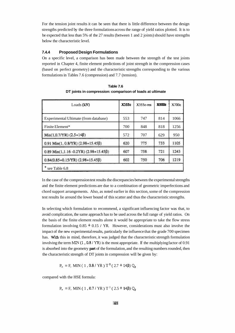
For the tension joint results it can be seen that there is little difference between the designstrengths predicted by the three formulations across the range of yield ratios plotted. It is tobe expected that less than 5% of the 27 results (between 1 and 2 joints) should have strengthsbelow the characteristic level.
7.4.4 Proposed Design FormulationsOn a specific level, a comparison has been made between the strength of the test jointsreported in Chapter 4, finite element predictions of joint strength in the compression cases (based on perfect geometry) and the characteristic strengths corresponding to the variousformulations in Tables 7.6 (compression) and 7.7 (tension).
Table 7.6DT joints in compression: comparison of loads at ultimate
Loads
* see Table 6.8
Experimental Ultimate (from database)
Finite Element*
In the case of the compression test results the discrepancies between the experimental strengths
and the finite element predictions are due to a combination of geometric imperfections and
chord support arrangements. Also, as noted earlier in this section, some of the compressiontest results lie around the lower bound of this scatter and thus the characteristic strengths.
In selecting which formulation to recommend, a significant influencing factor was that, to
avoid complication, the same approach has to be used across the full range of yield ratios. Onthe basis of the finite element results alone it would be appropriate to take the flow stressformulation involving 0.85 + 0.15 YR. However, considerations must also involve theimpact of the new experimentalresults, particularly the influence that the grade 700 specimenhas. this in mind, therefore, it was judged that the characteristic strength formulation involving the term is the most appropriate. If the multiplying factor of 0.91is absorbed into the geometry part of the formulation, and the resulting numbers rounded, then
the characteristic strength of DT joints in compression will be given by:
553
700
572
P,, = F, MIN 1 YR ) T ( 2.7 +
compared with the HSE formula:
747
848
707
P,, = F, MIN ( 1 YR ) T ( 2.5 +
814
818
629
1066
1256
950

The changes suggested have minimal impact on practice, but at the higher yield ratios allow about 16% increase in characteristic strength.
Table 7.7DT joints in tension: comparison of loads at ultimate
and characteristic levels for test dimensions
Loads lExperimental Ultimate (from database)
Experimental Crack
Experimental
from Yura deformation limit*
Finite Element
from Yura deformation limit*
* based on length of 2 braces + chord diameter
For tension joints (Table 7.7) it is seen that all characteristic strengths lie below the values
attained in the experiments. The order of characteristic strengths resulting from the three
proposed formulations is the same for the 355 and 700 grade joints, but differs for the grade
500 joint. There is little to choose between the formulations in the same sense as thecompression data given earlier, and for consistency it was decided to also adopt theformulation involving ( 1 YR ). If the multiplying factor of 0.74 is absorbed into
the geometry part of the formulation, and the resulting numbers rounded, then the
characteristic strength of DT joints in tension will be given by:
P,, = F, MIN ( 1 YR ) T ( 7 +
compared with the HSE formula:
From a practical standpoint the changes suggested are minimal, but at the higher yield ratios allow about a 12% increase in characteristicstrength over what is currently allowed in practice.

joints in compression
joints in tension
31.O%
0.5 0.6 0.7 0.8 0.9
ratiolimit limit)
Figure 7.1
Variation of normalised strength mean and COV for compression and tension loadedjoints in the DT database: yield ratio limit approach

0.7
0.75
0.
8 0.
85
0.9
0.95
1
1.05
1.1
Yiel
dra
tio55
065
075
0
Yiel
dst
reng
thFy
Figu
re7.
2D
Tco
mpr
essi
onjo
ints
tren
gth
vers
us y
ield
ratio
and
yie
ld s
tren
gth
from
fini
te e
lem
ent a
naly
ses

DT joints in compression
1.6
1.4
m
1.2M + =m =W 1
W
0.60.5 0.6 0.7 0.8 0.9 1
Yield ratio YR
DT joints in tension
0.5 0.6 0.7 0.8 0.9 1Yield ratio YR
Experimental
=
= +
Figure 7.3
Comparisonbetween the proposed design formulations and the experimental results from the DT static strength database


8. CONCLUSIONS
MATERIALS SURVEY
Conventional grade 355 plate steel is widely available, the majority of respondentsto the materials survey also produce one or more high strength structural steel plate grades for offshore use.
The processing routes and propertiesof structural steels have changed considerably over the last fifteen years. Three processing routes are used: normalising, TMCP(both for lowest strengths) and (very highest strength grades).
Other improvements in steel making and processing have permitted improved control over giving highly-grained steels of lean chemistry and, consequently, excellent weldability and toughness.
An area of concern was raised concerning the matching of weld and parent plate. Given the distributionsof yield strength of both, the probability does exist that weldsmay be undermatched.
The yield ratio of steel increases as yield strength increases. Values of - 0.75are typical for normalised grade 355 steels, whilst for steels in the range420 460 ratios between 0.75 and 0.85 may be found. Very high strengthsteels of grades 690 and above possess yield ratios ranging 0.90 to 0.95.
Elongation values vary grade to grade and tend to decrease with increasingstrength. For grades 355 and 450 minimum values are 22-25%. Forgrade 690, the value dropped to but typical values are in the range 14% - 18%.
There is no significant impediment to the use of high strength steels up to 450 grade.Grade 690 may require further characterisation, particularlyweldability studies, ifit is to be accepted in general offshore structural service. The welding and subsequent testing of the prototype scale joints used in this project has gone some way to confirming the weldability of the higher steel grades.
JOINT TESTING
All specimens loaded under compression failed in an asymmetric way, except the Grade 355 specimen with a hot rolled chord. The hot rolled chord specimen showeda higher normalised ultimate load than the cold rolled specimen of the same steel grade.
None of the compression specimens showed cracks until the end of the test.
All of the tension specimens failed in a ductile way. The cracks started at about50% of the ultimate load.
Notwithstandingthe unexpected failure mode in some cases of compression loadingdue to geometric imperfections, the joints performed in a consistently acceptablemanner (without brittle across all steel grades tested: obvious advantages, in terms of strength gain, were obtained from using the higher steel grades.
Minor concerns were raised in the fabrication of the high grade tension specimens by the fact that the welding procedure was adapted from that normally used for 30mm thick plate to the mm thick specimens. It may be that as thickness is reduced
may be experienced in achieving overmatching.
MATERIAL TESTING
There is no significant difference between the tensile strength (R,,,) of the flat plateand the cylindrical tensile specimens.
The flat plate tensile specimens give a lower yield strength than the cylindrical specimens.
The cylindrical tensile specimens showed no significant difference in yield strengthbetween the longitudinal and circumferential directions.
The cylindrical tensile specimens in the circumferential direction gave the most appropriate diagram for use in the FE calculation.
Although the weld metal in the high strength steel specimens was slightlyundermatched, the weld in the tubular joint did not fail because the stressdid not occur in the weld, but in the parent material.
DATABASE ANALYSIS
The tubular joint static database contained information on 687joints, 93% of which had material yield strengths that were less than or equal to 450
619 of those had documented material yield and ultimate strengths, of which 474(76.6%) had material yield strengths in excess of 0.7 times the material ultimatestrengths. The range of yield ratios was between 0.5 and
Yield ratio was found to be more strongly correlated with yield thanultimate High yield ratios were synonymous with, but not exclusive to, high strength steels. High yield ratios also occurred very commonly for low strengthsteels, where a high scatter of ratio was also evident. These latter facts may be related to the age of the steels in the database.
There were 120 DT joints in the screened database of which 101 had documentedyield and ultimate material The range of yield ratios was between 0.55and

8.4.5 Of the 74 compression DT joints, 68 (91.9%) had material yield strengths largerthan 0.7 times the ultimate the corresponding for the 27 tension DT joints was 24
8.4.6 A similar pattern to that of the unscreened database was exhibited by the DT joints
regarding yield ratio.
8.4.7 The least data on DT joints lies in the range 0.6 0.9; however, the test joints within the current project 0.82) have contributedsignificantly to the alleviationof this deficiency.
8.4.8 For DT joints in compression the HSEmean joint formula with a limitation on material yield ratio of 0.7 led to a lower-bound to the capacities in the screeneddatabase and a larger scatter compared with a yield ratio restriction of 1.0 (ie. unrestricted use of yield strength).
These features were repeated for tension joints except that the estimate and scatter were worse than was the case for the compression joints.
8.5 FINITE ELEMENT ANALYSIS OF DT JOINTS
8.5.1 Primary analyses of DT joints in compression, using material characteristics fromtension tests of 355, 500 and 700 grade steels supplied by a steel producer andnominal of the test specimens, revealed a yield ratio dependence for joint
that indicated a yield ratio limit of around 0.8.
8.5.2 For a DT joint in compression with a grade 355 yield there was little difference between the load-deflection responses (and hence the joint strengths) obtained from the actual material stress-strain curve (involving a yield plateau followed by strain hardening) and an idealised elastic-perfectly plastic stress-straincurve.
8.5.3 Aside from the specific point regarding strength (which cannot easily be predictedfinite element analysis), load-deflection responses for a DT joint in tension
using the different stress-strain curves for 355 grade steel, indicated in 8.5.2 above,were also very similar.
8.5.4 Secondaryanalyses of DT joints indicated that the mesh density used in the primary analyses, involving eight elements located along the chord-brace intersection linein a one-eighth model was of suitable accuracy for usage.
8.5.5 Imperfection studies (involving chord ovalisation, and brace centreline eccentricities and angular showed that for tension-loaded joints, the imperfections considered had a negligible effect on response.
For compression joints the brace centreline imperfections were shown to have a significant impact in lowering joint but reductionswere strongly dependenton the flexibility of the brace end or chord end support arrangements.
Secondary analyses of DT joints, using models that were geometrically identical tothe test specimens and material properties from tensile coupon tests on actualmaterials used, revealed that for joint strengths in compression a yield ratio limit ofaround 0.8 was implied.
In overall terms, the finite element analyses successfully replicated the test joint behaviour; they isolated and quantifiedgeometric imperfection effects fiom purelymaterial ones, and provided a calibrated numerical means for systematicexaminationof material effects in later Activities.
Finite element models of the sort used here are made to predict the overalldeformation behaviour. They are very successful in the case of compression joints.The simulationof the behaviour of tension joints is more limited because it requiresdetailed prediction of strain distributions, cracking and tearing. The latter twofeatures require much more sophisticated finite element modelling than the scopeof the present project has allowed.
DESIGN RECOMMENDATIONS
The DT compression joint static strength database was analysed using three different material formulations. The optimised values of parameters in the formulations ledto significant improvements in the COV of of experimental strengthdivided by mean predicted strength over the material formulation currently in use(see Table 8.1, columns a, b, c and d).
The DT tension joint static strength database was analysed using two differentmaterial formulations. The optimised values of parameters in the formulations led to marginal changes in the of the distribution of experimental strength divided by mean predicted strength over the material formulation currently in use, but improvements in distribution mean were obtained (see Table 8.1, columns g and
From a large number of compression finite element analyses undertaken on a fixedjoint geometry using a variety of material stress-strain curves generated systematically fiom a Ramberg-Osgood approach, it was found that joint strength was linearly related to material yield strength and yield ratio, but was not significantly affected by strain ratio (ratio of at ultimate stress to yield strain).
of yield plateau also reduced joint strength but this effect has not yet beenquantified fully.
From a finite element database constructed fiom the results just referred to, and a selection of those performed in Activity 5, a further material formulation wasapplied and proved to be an good predictor of compression joint strength. An optimised version of this, derived fiom the DT joint static strength database,

provided a COV of the distribution of experimental divided by meanpredicted similar to those the other new formulations (see Table 8.1, column e).
Table 8.1Comparison of material strength formulations F, F,
Compression F, F,
8.6.5 Three mean strength equations were suggested for DT joints under compression and tension, as follows:
Tension F, F,
MEAN
COV
. compression
P,= F, T2 (2.98 + 15.458)
P, 1.16 0.2 (2.98 + 15.458)
P,= F, (0.85 + (2.98 + 15.458)
tension
(l ,
8.6.6 Characteristic strength equations, based upon the lower 5% percentiles ofnormal of experimental strength divided by mean predicted foreach of the mean strength equations given above, and related to the experimental results this project, were recommended as follows:
1.01
10.65
K = 0.7
1.19
12.65
compression
K 0.8
10.77
P,, = F, (2.7
1-0.2
1.25
10.61
tension
P,, = F, T2 (7 +
75
0.945-
1.33
10.61
1.01
29.96
(1, KNR)
1.30
28.53
1.18
28.19

These represent a change from a 0.7 limit on material yield ratio to a value of 0.8.
8.6.7 In overall terms, the work has rigorously demonstrated through the combination oftests, finite element analysis and database analysis that conservatism can be safetyreduced, enabling wider use of high strength steels.

9. REFERENCES
Billington, C J. 'Possibilities for weight reduction in offshore topside structures',Proceedings of Offshore Weight Engineering Conference, London, 1987.
Billington, C J. 'The potential use and advantages of high strength and specialsteels offshore', Proceedings of Conference on Recent InternationalDevelopments', London, 1988.
Bond, H et al. 'Light weight design of offshore topside steel structures', Project No 83-3345, Stockholm, 1985.
GT Associates. 'High strength structural steels - a European review', Report EUR11761 for the Commission of the European Communities Technical SteelResearch Programme, Contract ECI 1467-86, 1988.
European Coal and Steel Community Seminar. 'Future steel requirements',London,December 1992
Lessells. J et al. 'The present state of technical knowledge of offshore structuralsteels and future material requirements', Study Group Report for the Commissionof the European Communities Technical Steel Research Programme, Contract
American Petroleum Institute. Recommended practice for planning, designing andconstructing fixed offshore platforms - load and resistance factor design', RP
1st Edition, July 1993.
Health and Safety Executive. 'Offshore installations: Guidance on design andconstruction', 4th Edition. 1990, plus amendments 1992. [Document withdrawn from 30 June 1998, as stated in HSE - OSD Operations Notice 27, revised andissued August
Marshall, P W. 'A review of American criteria for tubular structures and proposed revisions', 1977.
Rodabaugh, C. 'Review of data relevant to the design of tubular joints for use in fixed offshore platforms', Welding Research Council Bulletin 256, 1980.
K et al. 'Experimental study on local failure of chords in tubular trussjoints', Technology Report of the University, 18, 1968.
Health and Safety Executive. 'Background to new static strength guidance fortubular joints in steel offshore structures', Offshore technology Report, 89308, HMSO. 1990.

Cranfield University (formerly Institute of Technology). Managed Programme onHigh Strength Steels in Offshore Engineering, 1985-1987, 1987-1989, 1992-1994.
Dowling, P J, et al. 'Structural steel design', 1988.
Healy, B E and Zettlemoyer, N. 'In-plane bending strength of circular tubular
joints', Proceedings of Fifth International Symposium on Tubular Structures, ed. M
G Coutie and G Davies, Spon, 1993.
Lalani, M et al. 'The static strength and behaviour of joints in jack-up rigs', Proceedings of the Fourth International Conference on the Jack-up Platform,
London, 1993
Sakamoto, S et al. 'Static and fatigue strength of high tensile strength steel tubular
joints for offshore structuresi, The Sumitomo Search No 19, May 1978.
Kurobane, Y et al. 'Additional tests on tubular K-joints with CHS members understatic loads', XV-460-80, 1980.
Wilmhurst, S R and Lee M M K. 'Nonlinear study of ultimate strength oftubular multiplanar double K-joints', Proceedings of 12th International Conferenceon Offshore Mechanics and Arctic Engineering, Glasgow, 1993.
Joint Industry Project. 'Jack-up site assessment procedures - establishmentof an
internationalrecommended practice', Presentation by Noble and Associates
and project sponsors, City University, London, 1993.
W T et al. 'Steels for jack-up legs', In Recent Developments in Jack-Up
Platforms, Eds L F Boswell and C Blackwell Scientific Publications,London 1992.
Petersen, R I et al. 'Fatigue life of high steel plate elements with welded
attachments', Conference on fatigue under spectrum loading and in corrosive
environments, Copenhagen, 1993.
L, et al. 'Fatigue life of high strength steel tubular joints',
Conference on fatigue under spectrum loading and in corrosive environments,Copenhagen, 1993.
Stacey, A, Sharp, J V and King, R N. 'High strength steels used in offshore
installations', Offshore Mechanics and Arctic Engineering Conference, Florence,
1996.
Health and Safety Executive. 'Proposed revisions to fatigue guidance', including amendments, August

Billington, C J. 'Application of high strength steels in design of fixed offshorestructures', Conference on Safe Design and Fabrication of Offshore Structures,London, 1993.
Billington C J. The potential use and advantagesof high strength and special steels - offshore', Proceedings from Oil and Gas Production, Recent International
Technological Developments Conference, 1988.
Billingham J. 'Steel - A versatile advanced material in marine environments', Proceedings from Structural Materials in Marine Environments Conference,
London, 1994.
Healy J. 'Metallurgical considerations of the high yield to ultimate ratio in highstrength steels for use in offshore engineering', Proceedings from the OffshoreMechanics and Arctic Engineering Conference, Copenhagen, 1995.
Billingham J and Bolt H. The question of high ratio in highstrength steels', Report 951100, 1995.
The Marine Technology Directorate Limited. 'High strength steels in offshoreengineering', Publication 951100, 1995.
Pickering F B. 'Physical metallurgy and the design of steels', Applied SciencePublishers, 1978.
American PetroleumInstitute. 'Recommended practice for planning, designing and constructing fixed offshore platforms load and resistance factor design', R P2A, 1st Edition, July 1993.
Yura, J A et al. 'Ultimate capacity equations for tubular joints', Paper No
3690, Offshore Technology Conference, Houston, 1980.
Health and Safety Executive. 'Offshore installations: Guidance on design and construction', 4th Edition, 1990, plus amendments. [Document withdrawn from 30June 1998, as statedin HSE - OSD Operations Notice 27, revised and issued August19981.
Health and Safety Executive. 'Background to new static strength guidance for tubular joints in steel offshore structures', Offshore Technology Report, 89308, HMSO,
Ochi K et al. 'Basis for design of unstiffened tubular joints under axial braceloading', Document XV-561-84, Annual Assembly, 1984.
International Institute of Welding. 'Design recommendation for hollow sectionjoints'. XV-701-89, 1989.

Wardenier J et al. 'Design guide for circular hollow section (CHS) joints underpredominantly static loading', 1.
C P et al. 'Tubular joint strength formulations the importance forharmonisation', Society for Underwater Technology Conference on
Its Present and Future Role in Offshore Safety Cases, London, 1993.
BOMEL Limited. 'BOMEL Tubular Joints Design Guide, Chapter 3 StaticStrength', September
Canadian Standards Association (CSA). 'Steel Structures - OffshoreA National Standard of Canada. 1992.
Det Norske 'Rules for the Design, Construction and Inspection ofOffshore Structures', July 1993.
UEG. 'Design of Tubular Joints for Offshore Structures, Volume Publication1985.
from British Steel, BOMEL dated October
ABAQUS finite element system. Hibbett, and Sorenson Inc.
'Static behaviour of multiplanar welded joints in circular hollow sections', StevinReport 1991.
Health and Safety Executive. 'Background to new static strength guidance for tubular joints in steel offshore structures', Offshore Technology Report, 89308, HMSO, 1990.
Yura J A, Zettlemoyer N, Edwards I F. 'Ultimate capacity equations for tubularjoints', OTC Paper No 3690, Offshore Technology Conference, 1980
Private Communication, Langford Crockett, BOMEL.
Lalani, M et al. The static strength and behaviour of joints in jack-up rigs', Proceedingsof the Fifth International Conference on the Jack-up Platform, London,
Zettlemoyer, N. harmonisation of offshore guidance on strength of tubularjoints', Proceedings of the Sixth International Offshore and Polar EngineeringConference, Los Angeles, 1996.
A, et al. 'High strength steels used in offshore installations', Proceedings of15th International Conference on Offshore Mechanics and Arctic Engineering, Florence, 1996.
Baker, M J, 'Variability in the strength of structural steels. A study in structuralsafety', Part I , Technical Note April 1983.


Printed and published by the Health and Safety Executive C1 8/99