ISSN 1651-4416

SKB P-06-278

Oskarshamn site investigation

Production and respiration measurements in different vegetation types

Comparisons between a young pine stand, a wet forest, a fen, and an agricultural field

Elisabeth Lundkvist, Calluna AB

December 2006

Keywords: Respiration, Production, GPP, Vegetation, Wetland, AP PS 400-06-007.

This report concerns a study which was conducted for SKB. The conclusions and viewpoints presented in the report are those of the author and do not necessarily coincide with those of the client.

A pdf version of this document can be downloaded from www.skb.se

�

Abstract

The objective of the investigation was to estimate biological production and respiration within the soil and ground layer of four different vegetation types in the Oskarshamn area. The four types were a young pine stand, a wet forest (alder), a poor fen, and an agricultural field. The field measurements were done with a closed chamber attached to an environmental gas monitor for carbon dioxide. Soil temperature at 10 cm depth, air temperature, air concentration of carbon dioxide, and photosynthetic active radiation (PAR) were also measured.

Production measurements were performed in daylight, and respiration measurements were achieved through placing a black bucket over the transparent chamber in order to prevent radiation to reach the vegetation. The measurements were done six times from March to October 2006. The obtained data will be used in an ecosystem model of the Oskarshamn area, which is part of the site description.

The highest production was obtained in the agricultural field and the poor fen. Production in the young pine stand and the wet forest was near zero over the whole season. We think the poorly developed ground layers can explain this.

Respiration on the other hand was detectable in all areas and highest during summer months. Respiration exceeded production in all areas.

Respiration was generally zero in March, and increased over the season to become lower in the autumn again. However, respiration still occurred in the end of October in all areas while production by then was zero in all areas.

�

Sammanfattning

Syftet med undersökningen var att mäta produktion och respiration i mark och markskikt i fyra olika vegetationstyper. Studien genomfördes i mars–oktober 2006 i Laxemarområdet norr om Oskarshamn. De fyra vegetationstyperna var ung tallskog, ca 15–�0 år, alsumpskog, fattigkärr och åker med vallodling.

Mätningarna gjordes i en sluten kammare förbunden med en infraröd koldioxidmätare. Förutom halten koldioxid mättes också lufttemperatur, marktemperatur och solinstålning i form av PAR (strålning inom spektrat �00–700 nm, utnyttjas vid fotosyntesen).

Vi mätte produktion i dagsljus och respiration i mörker. Mörker åstadkoms genom att sätta en svart hink över den genomskinliga mätkammaren. Mätningarna gjordes vid sex tillfällen från mars–oktober och erhållna data kommer att användas i en ekosystemmodell över kolflöden i Oskarshamnsområdet.

De högsta produktionsvärdena uppmättes på åkermarken och i fattigkärret. I tallskogen och i sumpskogen var produktionen nära noll och det gick inte att se någon tydligt trend att produktionen ökade sommartid jämfört med tidig vår och sen höst. Fältskiktet var relativt klent i dessa områden och det kan förklara den låga produktionen.

Respirationen visade däremot ett entydigt mönster i alla områden, de första uppmätta värdena i mars låg nära noll, men ökade under mätperioden med ökande temperatur. De högsta värdena uppmättes sommartid. Respirationen översteg produktionen i alla områden. Respirationen pågick fortfarande i slutet av oktober, medan produktionen vid den tidpunkten åter var noll.

5

Contents

1 Introduction 7

2 Objectiveandscope 11

3 Descriptionoffieldequipment 1�

4 Execution 15�.1 General 15�.2 Notes about the instruments 15�.� Execution of field work 15�.� Data handling/post processing 16�.5 Analyses and interpretations 16�.6 Nonconformities 16

5 Results 175.1 Field activities 175.2 Production and respiration 18

5.2.1 Agricultural field 185.2.2 Young pine stand 215.2.� Wet forest 2�5.2.� Poor fen 25

5.� Summarising the results 27

6 References 29

7

1 Introduction

This document reports the results from production and respiration measurements in different vegetation types. This is one of the activities performed within the site investigation at Oskarshamn. The work was carried out in accordance with activity plan AP PS �00-06-007 (Table 1-1).

The exchange of CO2 from the ground to the atmosphere, deriving from living organisms’ pro-duction and respiration, gives a measure on the total autotrophic1 and heterotrophic2 respiration in the soil, and also gives a measure on the ground layer production. In earlier studies within the site investigations at Oskarshamn and Forsmark, production and respiration have been measured in both terrestrial and aquatic environments /Tagesson in press, Karlsson 2006/. This study complement existing site descriptions and models over the Oskarshamn area with data from additional vegetation types. The final aim is to generate information on the carbon cycle and flows between different carbon pools.

This report mainly deals with the concepts of respiration and GPP in the field and bottom layer, and the soil. The overall carbon flux between the ecosystem and the atmosphere is called the NEE (Net Ecosystem Exchange), which is a function of mainly three processes, Gross primary production (GPP) in vegetation, heterotrophic and autotrophic respiration. GPP refers to the total amount of energy fixed by plants. This energy can then be used by plants to generate new biomass; growing. So, the total uptake by plants of carbon through photosynthesis is GPP. Respiration, where carbon is released, is the sum of respiration from above ground vegetation, roots, mycorrhiza, and microbes. The instrument records values of respiration (in darkness, using a bucket). NEE (in sun light), for the field layer and the soil. GPP is derived by subtracting respiration from NEE. We compared the levels of respiration and production in four different vegetation types.

There are many different factors that control respiration and production, but temperature is a dominant factor, and hence production and respiration fluctuate seasonally. GPP is also affected by solar radiation that is used in photosynthesis (measured in the unit PAR in this study), while soil respiration in addition to temperature, is highly dependent on moisture /Kirschbaum 1995, Morén and Lindroth 2000/.

Table1‑1. Controllingdocumentfortheperformanceoftheactivity.

Activityplan Number Version

Respiration och produktion på våtmark, åkermark och i ungskog AP PS 400-06-007 1.0

1 Organism able to use CO2 as its only source of carbon, inorganic nitrogen and other elements as its sole starting materials for biosynthesis. 2 Organism that require organic compounds as carbon source. Achieved through consumtion.

8

The measurements in this study were done in four vegetation types (Figure 1-2):

1. Young pine stand. Tree and shrub layer dominated by pines (Pinus sylvestris) of different heights and ages (ca. 15–�0 years). Ground layer dominated by dwarf shrub and bracken.

2. Wet forest. Tree and shrub layer dominated by alder (Alnus glutinosa) and ground layer by grasses, mainly broad-leaved, and soft rush (Juncus effusus).

�. A poor fen. Shrub layer dominated by bog-myrtle (Myrica gale), with some birch (Betula pubescens and B. pendula) in the tree layer. Ground layer dominated by Sphagnum spp., Potentilla palustris, and thin leaved grasses.

�. Agricultural field. Temporary abandoned and sometimes used for hay production. The ground layer is dominated by grass and herbs. No tree or shrub layer.

Figure 1-1 shows an overview over the Oskarshamn site investigation area, and we measured CO2 concentrations deriving from activities in soil and ground layer in these areas from March to October 2006.

Figure 1‑1. Oskarshamn site investigation area. Overview over the four investigated areas where pro-duction and respiration was measured from March to October 2006. OKG nuclear power plant in the eastern part of the map.

9

Figure 1‑2. Photos from the four investigated sites where production and respiration was measured in the Oskarshamn area. A general view to the left and view of the ground layer to the right. a) Young pine stand, b) wet alder forest, c) poor fen area, and d) agricultural field.

a)

b)

c)

d)

11

2 Objectiveandscope

The objective of the investigation was to estimate production and respiration in four different vegetation types; a pine stand, a wet forest, a poor fen, and an agricultural field. The instrument, an infrared carbon dioxide gas monitor, was placed at the ground and measured production and respiration both from soil and ground layer. Temperature in the soil and in air was also measured. The purpose with the study was to complement earlier investigations with data from other vegetation types. The data will be used in an ecosystem model describing carbon flows in the Oskarshamn area.

Every site was visited six times from March to October. In each site measurements were done in eight fixed points and median values from each month is presented in the report.

1�

3 Descriptionoffieldequipment

We used an EGM-� environmental gas monitor for CO2, provided with a CPY-2 canopy assimi-lation chamber, for measuring carbon dioxide concentrations (Figure �-1). The instruments are from PP Systems and we used the /Operator’s manual 200�/ for EGM-�, version �.1�.

The CPY-2 chamber is provided with a light sensor measuring photosynthetic active light as PAR (µmol m-² sec-¹). The instrument also measures air temperature within the chamber. Air from the chamber is transported to the EGM-� via tubes, and the EGM-� uses infrared light to analyse CO2 concentration (gases such as CO2 absorbs photons in the infrared range).

The EGM-� also registers atmospheric pressure and atmospheric carbon dioxide concentration.

Data are stored in the EGM-� and easily transferred to a computer.

Soil and air temperatures were measured with a digital thermometer with accuracy ± 0.5°C.

Figure 3‑1. EGM-4 gas monitor for CO2 to the left, and CPY-2 chamber for closed systems to the right. Both instruments from PP Systems.

15

4 Execution

4.1 GeneralThe investigation took place at four different ecosystems in the region of the Laxemar investiga-tion area. The Laxemar investigation area is situated 25 km north of Oskarshamn in southern Sweden and is part of the investigations by SKB for a repository of nuclear waste.

We measured production and respiration in four vegetations types six times from the end of March to the end of October 2006. In each of the four areas, there were eight fixed points, which were given unique ID’s using GPS. The measurements took place at these points (in total �2 points, 8 at each of the four sites). We followed the operator’s manual for the EGM-�, and also used supplementary information from the staff at SKB, based on experiences of the instrument.

We measured soil and air temperature in each area in addition to the parameters measured by the instrument.

After each field session, data from the instrument was transferred from the instrument to a computer, and then transferred to SKB’s database SICADA. Data are traceable in SICADA by the activity plan number.

4.2 NotesabouttheinstrumentsSome specific notes about the instruments are worth mentioning. The EGM-� battery was charged before each measuring period (i.e. each month). The instrument was on for ca. 6 hours each field session and there were no problems with low battery level in spite of very different weather situations.

The EGM-� contains a column with soda lime (to clear entering air from CO2), and this was replaced each month before measuring according to the manual.

The EGM-� is sensible for moist and hence, it was never placed directly on the ground, and in moist or rainy weather it was sheltered by an umbrella.

The CPY-2 was also sensible for moist, and when the chamber got wet inside, the instrument did not record data in a correct way. In those cases, the chamber needed to be carefully dried with a towel or paper before measuring again.

4.3 ExecutionoffieldworkIn field, the instruments were connected and prepared according to the manual. After identifying the exact spot with GPS, the chamber was placed on the ground. The first measurement on each plot was done in daylight (respiration), and the second (on the same plot) was in dark. To get dark conditions, we placed a black plastic bucket over the chamber so that no sunlight would reach the vegetation inside the chamber.

Each measurement took ca. 2 minutes, which means � minutes on each plot and �2 minutes in each vegetation type. There was some handling time between the measurements, e.g. between measuring in light and dark, and also before starting at a new point, the chamber was held in the air, the fans inside flushed the chamber and it self-calibrated. In total, measuring at one area roughly took 60–90 minutes.

16

Along with measuring in light and dark at the eight plots, we measured soil and air temperature at each spot, took photos of the area, noted weather conditions and dominating vegetation in the ground layer.

4.4 Datahandling/postprocessingThe data were recorded in the EGM-�. The machine could store half of the values for each session (ca. 1,000 values), so it had to be emptied once. The data were easily transferred to a computer.

The data were converted to MS Excel data and further processed. After each field session, the data were copied into the SICADA template and sent to SKB along with activity diary and photos.

4.5 AnalysesandinterpretationsData of respiration and production (GPP) were analysed further. We used the last recorded value of respiration and GPP in each spot. This value is obtained after measuring during two minutes. When plotting the eight values for each spot, it was obvious that data were not normally distributed so non-parametric testing was necessary.

We performed Kruskal-Wallis test (comparable to ANOVA), to test for differences between medians (test for differences between the months in each area). We also performed a non-parametric multiple comparison test to see between which pairs we had significant differences. All analyses and graphs were made in Statistica 7.

We did two box-whisker diagrams for each vegetation type, one for respiration and one for GPP. Each diagram consists of six boxes, one for each month (based on eight values) we measured in field, which makes it easy to observe seasonal changes.

In the box-whisker diagrams the median, 25–75% percentiles, and outliers are illustrated. In the area between 25–75% lies 50% of the data, and hence it is quite probable that the “true mean” is found within this area.

4.6 NonconformitiesThe earlier mentioned sensitivity for moist (both EGM-� and CPY-2 machines) might have affected the results. The message ”non-linear fit” now and then was displayed under moist conditions, but after drying the chamber, we did not meet any difficulties with the measuring procedure.

At the last occasion, the EGM-� did not register light (PAR) at the young pine forest. It was rather cloudy and not very light conditions, but probably something was wrong with the machine at that moment. Later, it worked again. Unfortunately, you cannot see what data is registered until processing the data in a computer. We got no indication in field that PAR was not recorded.

Concerning temperature, due to a misunderstanding we only measured soil temperature at one point in each area at the first two occasions in March and May, but from June and forward, we measured temperature at each single spot (in total �2 spots).

We took no soil samples from each area as indicated by the activity plan (Table 1-1) since SKB decided not to perform this activity.

17

5 Results

5.1 FieldactivitiesThe four areas were visited six times, and each time we registered dominating vegetation. It did not change over the season and the most common species are presented in Table 5-1.

The agricultural field was dominated by grasses. In March, the soil was naked and not until June the ground was covered with grass.

The pine stand had a weak ground layer, and it did not change much during the growing season since it mainly consisted of dwarf shrub.

The wet forest was really wet in March and May, but dried to a large extent during June and was dry throughout our measuring period.

The poor fen was wet during March, May and June, but gradually dried during summer. However, it was still wet but no water trickled around the boots when stepping on the ground.

The most notable weather condition (Table 5-2) was at the first occasion in March, when the ground was covered with �0 cm snow. Otherwise, soil temperature during summer was gener-ally lowest at the pine stand and rather equal at the other areas. The lowest soil temperature in October was found in the agricultural field, and since the ground was partly naked, heat quickly left the ground.

The forested areas logically received less solar radiation than did the agricultural and fen areas. Within a single measurement, the PAR value could fluctuate much depending on clouds temporarily covering the sun, hence the largest variations was in sunny weather.

Table5‑1. Thefourinvestigatedareaswhereproductionandrespirationwasmeasured.

Investigatedareas ASMcode x‑coordinate y‑coordinate Dominatingvegetation

Agricultural field ASM000015 6366698 1548110 Phleum pratense Lolium perenne

Young pine stand ASM000016 6368774 1545700 Pinus sylvestris Vaccinium vitis-idaea Calluna vulgaris Pteridium aquilinium mosses

Wet forest ASM001434 6367880 1551067 Alnus glutinosa Grasses Juncus effusus Filipendula ulmaria

Poor fen ASM001443 6363425 1540919 Myrica gale Sphagnum spp. Carex spp.

18

Table5‑2. Mean±stddev.forPhotosyntheticActiveRadiation(PAR)basedonNnumberofobservations.SoiltemperaturebasedononevalueperareainMarchandMay,andeightvaluesperareainJune–October.Airtemperaturebasedononevalueperarea.

March30–31 May10 June21 Aug23 Sept26 Oct26

AgriculturalN

PAR µmol m-² sec-¹

Air temp °C

Soil temp °C

40 cm snow

216

215 ± 41

7

1.4

Sunny

209

1,579 ± 208

18.5

10.4

Clouds/rain

136

141 ± 48

20

16 ± 0.1

Sunny

161

646 ± 520

22

17.5 ± 0.9

Sunny

216

968 ± 150

15

16.7 ± 0.2

Rain

213

52 ± 12

4.5

6.8 ± 0.4

PinestandN


Air temp °C

Soil temp °C

40 cm snow

216

187 ± 66

10

1.4

Sunny

216

482 ± 342

19.5

9.5

Clouds/rain

175

122 ± 40

21

13.4 ± 0.2

Sunny

152

72 ± 36

18

13.9 ± 0.6

Sunny

183

51 ± 16

9.5

13.2 ± 0.2

Rain

209

0*

7

9.3 ± 0.3

WetforestN


Air temp °C

Soil temp °C

40 cm snow

216

152 ± 37

10

2.5

Sunny

216

278 ± 163

14

8.4

Clouds/rain

168

78 ± 37

18.5

15.6 ± 0.4

Sunny

181

52 ± 25

20

16.4 ± 0.4

Sunny

216

63 ± 39

17

16.3 ± 0.3

Rain

216

24 ± 16

11.5

10.4 ± 0.3

PoorfenN


Air temp °C

Soil temp °C

40 cm snow

216

89 ± 27

10

4

Sunny

206

1,438 ± 197

21

10

Clouds/rain

207

153 ± 54

17

16.7 ± 0.4

Sunny

145

904 ± 679

23.5

16.1 ± 0.2

Sunny

187

341 ± 245

21.5

16.4 ± 0.2

Rain

215

116 ± 47

12

10.2 ± 0.1

* No light values recorded by the EGM-4 at this point.

5.2 Productionandrespiration5.2.1 AgriculturalfieldThe production in the agricultural field was only fairly consistent with the growing season (Figure 5-1). We had expected the largest production to be in June and August. However, from May to September we noticed a production, and in March and October the values were close to zero. Note that production means uptake of carbon dioxide and hence negative values of the y-axis in Figure 5-1.

In spite of the large error bars, March and October differed from both May and August. The summer months May to September did not differ significantly from each other (Table 5-�).

19

Table5‑3. Multiplecomparisonsofp‑valuesfromGPPmeasurementsinanagriculturalfield.Kruskal‑Wallistest:H(5,N=48)=31.53,p=0.00.

March May June Aug Sept

MarchMay 0.01

June 1.00 1.00Aug 0.00 1.00 0.77Sept 0.57 1.00 1.00 1.00Oct 1.00 0.00 0.44 0.00 0.17

Figure 5‑1. Production as GPP (g CO2 / m2·h–1) in an agricultural field in the Laxemar area, Oskarshamn. Negative values mean production (uptake of carbon dioxide).

20

Respiration in the agricultural field was highest during June and August, and lowest in March and October as expected (Figure 5-2). March and October differed significantly from June and August (Table 5-�).

Table5‑4. Multiplecomparisonsofp‑valuesfromrespirationmeasurementsinanagri‑culturalfield. Kruskal‑Wallistest:H(5,N=48)=40.96,p=0.00.


MarchMay 0.12

June 0.00 0.27Aug 0.00 0.15 1.00Sept 0.12 1.00 0.27 0.15Oct 1.00 1.00 0.01 0.00 1.00

Figure 5‑2. Respiration (g CO2 / m2·h–1) in an agricultural field in the Laxemar area, Oskarshamn. Positive values mean respiration (release of carbon dioxide).

21

Figure 5‑3. Production as GPP (g CO2 / m2·h–1) in a young pine stand in the Laxemar area, Oskarshamn. Negative values mean production (uptake of carbon dioxide).

5.2.2 YoungpinestandProduction was low over the whole season and there were only significant differences in production between June and March. Otherwise, the months did not differ from each other statistically (Figure 5-�, Table 5-5). The ground layer was poorly developed and naked soil or lichen covered a large part of the ground. This fact might explain the result.

Table5‑5.Multiplecomparisonsofp‑valuesfromGPPmeasurementsinayoungpinestand.Kruskal‑Wallistest:H(5,N=48)=12.35,p=0.03.


MarchMay 0.21

June 0.05 1.00Aug 1.00 1.00 1.00Sept 1.00 1.00 0.35 1.00Oct 1.00 1.00 0.81 1.00 1.00

22

Respiration in the young pine stand was more obvious than the production was (Figure 5-�). It was highest during August, but rather high also during June, September, and October.

May, June and August differed from March, and May also differed from June and August (Table 5-6). It seems as respiration continued longer on a higher level in the pine stand than in the other areas.

Table5‑6. Multiplecomparisonsofp‑valuesfromrespirationmeasurementsinayoungpinestand. Kruskal‑Wallistest:H(5,N=48)=32.83,p=0.00.


MarchMay 1.00

June 0.00 0.05Aug 0.00 0.01 1.00Sept 0.01 0.49 1.00 1.00Oct 0.16 1.00 1.00 0.45 1.00

Figure 5‑4. Respiration (g CO2 / m2·h–1) in a young pine stand in the Laxemar area, Oskarshamn. Positive values mean respiration (release of carbon dioxide).

2�

5.2.3 WetforestIn the wet forest, production seemed to be highest in May, and it differed from March, June and October, but not from the other months. (Figure 5-5, Table 5-7). Naked soil covered a large part of the area in spite of the fact that there was grassy vegetation. This might explain why production was low during summer months June and August.

Table5‑7.Multiplecomparisonsofp‑valuesfromGPPmeasurementsinawetforest.Kruskal‑Wallistest:H(5,N=48)=21.54,p=0.00.


MarchMay 0.00

June 1.00 0.03Aug 0.93 0.17 1.00Sept 1.00 0.07 1.00 1.00Oct 1.00 0.01 1.00 1.00 1.00

Figure 5‑5. Production as GPP (g CO2 / m2·h–1) in a wet forest on Äspö, Oskarshamn. Negative values mean production (uptake of carbon dioxide).

2�

The respiration pattern was consistent with climate, and was highest during the warmest months June and August (Figure 5-6). Respiration in June and August differed from March and October (Table 5-8). There was still an active ecosystem in October as respiration occurred.

Table5‑8. Multiplecomparisonsofp‑valuesfromrespirationmeasurementsinawetforest. Kruskal‑Wallistest:H(5,N=48)=38.16,p=0.00.


MarchMay 0.06

June 0.00 1.00Aug 0.00 0.32 1.00Sept 0.09 1.00 0.82 0.21Oct 1.00 1.00 0.02 0.00 1.00

Figure 5‑6. Respiration (g CO2 / m2·h–1) in a wet forest on Äspö, Oskarshamn. Positive values mean respiration (release of carbon dioxide).

25

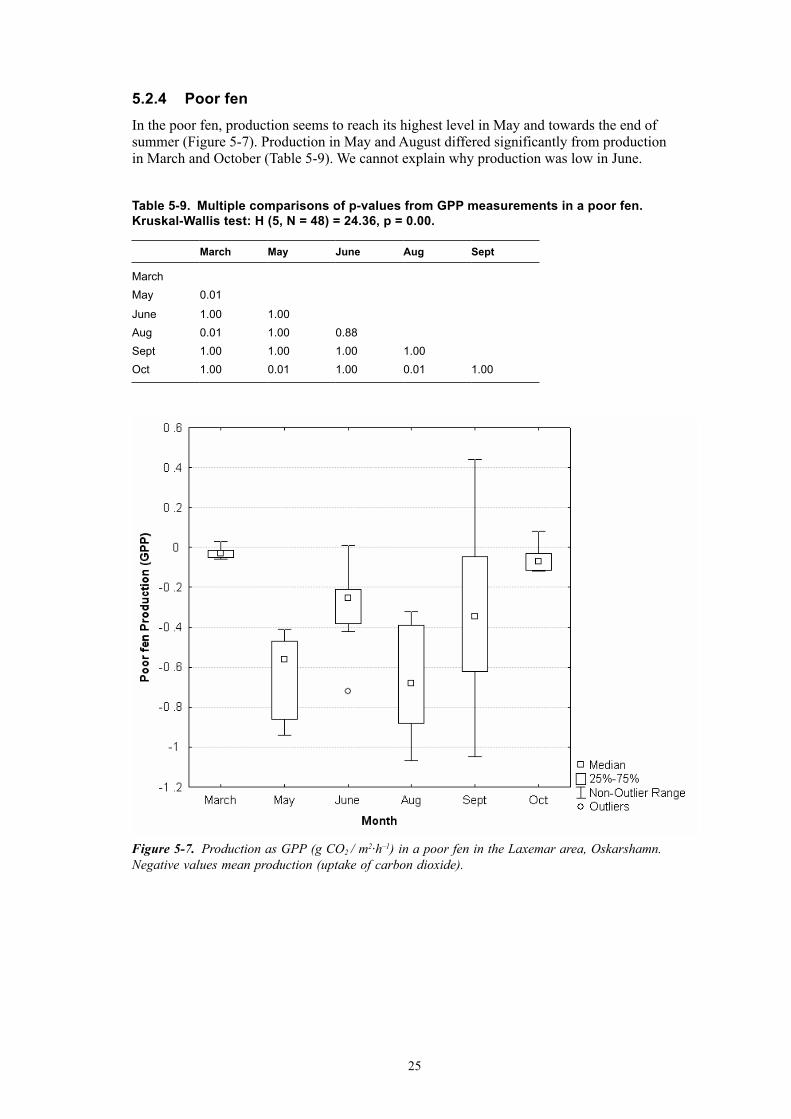
5.2.4 PoorfenIn the poor fen, production seems to reach its highest level in May and towards the end of summer (Figure 5-7). Production in May and August differed significantly from production in March and October (Table 5-9). We cannot explain why production was low in June.

Table5‑9. Multiplecomparisonsofp‑valuesfromGPPmeasurementsinapoorfen.Kruskal‑Wallistest:H(5,N=48)=24.36,p=0.00.


MarchMay 0.01

June 1.00 1.00Aug 0.01 1.00 0.88Sept 1.00 1.00 1.00 1.00Oct 1.00 0.01 1.00 0.01 1.00

Figure 5‑7. Production as GPP (g CO2 / m2·h–1) in a poor fen in the Laxemar area, Oskarshamn. Negative values mean production (uptake of carbon dioxide).

26

As in the other areas, respiration in the poor fen showed a clear pattern, with highest values during summer (Figure 5-8). From May to September, production was significantly higher than in March, and August and September also differed from October (Table 5-10).

Table5‑10. Multiplecomparisonsofp‑valuesfromrespirationmeasurementsinapoorfen. Kruskal‑Wallistest:H(5,N=48)=36.99,p=0.00.


MarchMay 0.02

June 0.03 1.00Aug 0.00 0.74 0.59Sept 0.01 1.00 1.00 1.00Oct 1.00 0.16 0.21 0.00 0.05

Figure 5‑8. Respiration (g CO2 / m2·h–1) in a poor fen in the Laxemar area, Oskarshamn. Positive values mean respiration (release of carbon dioxide).

27

5.3 SummarisingtheresultsThe highest production values were derived from the agricultural field and the poor fen. In the young pine stand and the wet forest, we could only see a weak trend that production increased with increasing temperature or greater influx of solar radiation. The levels were close to zero over the whole season. In the pine stand, the poorly developed ground layer might explain the low production. In the wet forest, naked soil covered a substantial part of the ground even though there was rather dense grass vegetation.

Respiration on the other hand was detectable in all areas. Respiration was zero or near zero in March, increased to reach its highest levels in the summer months, and became lower again in the autumn. Respiration exceeded production in all areas.

Respiration still occurred in the end of October in all areas, while production by then was zero in all areas.

In this study it is clear that respiration is highly dependent on temperature, perhaps both in soil and in air, while production is mainly dependent on solar radiation and on the fact that there is a field or bottom layer to perform any production.

29

6 References

KarlssonS,2006. Forsmark site investigation. Production and respiration measurements in Lake Bolundsfjärden 2005. SKB P-06-�1, Svensk Kärnbränslehantering AB.

KirschbaumMUF,1995. The temperature dependence of soil organic matter and the effect of global warming on soil organic C storage. Soil Biology and biochemistry. 27:75�–760.

MorénA-S,LindrothA,2000. CO2 exchange at the floor of a boreal forest. Agricultural and Forest Meteorology. 101:1–1�.

Operator’sManual,2003. EGM-� Environmental Gas Monitor for CO2. Version �.1�. PP Systems, Hertfordshire, UK.

TagessonT, (inpress). High soil carbon efflux rates in several ecosystems in Southern Sweden, Boreal Environment Research.

Oskarshamn site investigation - Production and respiration

Documents

Transcript of Oskarshamn site investigation - Production and respiration