Orion Optical Navigation Progress Toward Exploration

Mission 1

Greg N. Holt∗, Christopher N. D’Souza†, and David Saley‡

NASA Johnson Space Center, 2101 NASA Parkway, Houston, TX, 77058

Optical navigation of human spacecraft was proposed on Gemini and implemented suc-cessfully on Apollo as a means of autonomously operating the vehicle in the event of lostcommunication with controllers on Earth. The Orion emergency return system utilizingoptical navigation has matured in design over the last several years, and is currently un-dergoing the final implementation and test phase in preparation for Exploration Mission1 (EM-1) in 2019. The software development is past its Critical Design Review, and isprogressing through test and certification for human rating. The filter architecture uses asquare-root-free UDU covariance factorization. Linear Covariance Analysis (LinCov) wasused to analyze the measurement models and the measurement error models on a repre-sentative EM-1 trajectory. The Orion EM-1 flight camera was calibrated at the JohnsonSpace Center (JSC) electro-optics lab. To permanently stake the focal length of the cameraa 500 mm focal length refractive collimator was used. Two Engineering Design Unit (EDU)cameras and an EDU star tracker were used for a live-sky test in Denver. In-space imagerywith high-fidelity truth metadata is rare so these live-sky tests provide one of the closestreal-world analogs to operational use. A hardware-in-the-loop test rig was developed inthe Johnson Space Center Electro-Optics Lab to exercise the OpNav system prior to inte-grated testing on the Orion vehicle. The software is verified with synthetic images. Severalhundred off-nominal images are also used to analyze robustness and fault detection in thesoftware. These include effects such as stray light, excess radiation damage, and specularreflections, and are used to help verify the tuning parameters chosen for the algorithmssuch as earth atmosphere bias, minimum pixel intensity, and star detection thresholds.

I. Background

Optical navigation of human spacecraft was proposed on Gemini and implemented successfully on Apolloas a means of autonomously operating the vehicle in the event of lost communication with controllers

on Earth. This application was quintessentially summarized in the epilogue to Battin.1 It shares a historywith the “method of lunar distances” that was used in the 18th century and gained some notoriety after itsuse by Captain James Cook during his 1768 Pacific voyage of the HMS Endeavor. The Orion emergencyreturn system utilizing optical navigation has matured in design over the last several years, and is currentlyundergoing the final implementation and test phase in preparation for Exploration Mission 1 (EM-1) in 2019.The software development is being worked as a Government Furnished Equipment (GFE) project deliveredas an application within the Core Flight Software of the Orion camera controller module.

A. Concept of Operations

The Orion optical navigation system uses a body fixed camera, a decision that was driven by mass andmechanism constraints. The general concept of operations involves a 2 hour pass once every 24 hours,with passes specifically placed before all maneuvers to supply accurate navigation information to guidanceand targeting. The pass lengths are limited by thermal constraints on the vehicle since the OpNav attitudegenerally deviates from the thermally stable tail-to-sun attitude maintained during the rest of the orbit coast

∗NASA Orion Navigation Lead, Aeroscience and Flight Mechanics Division, EG6, AIAA Senior Member†Navigation Technical Discipline Lead, Aeroscience and Flight Mechanics Division, EG6, AIAA Associate Fellow‡Orion Navigation Hardware Subsystem Manager, Aeroscience and Flight Mechanics Division, EG2

1 of 12

American Institute of Aeronautics and Astronautics

https://ntrs.nasa.gov/search.jsp?R=20180000595 2018-08-17T08:32:15+00:00Z

phase. Calibration is scheduled prior to every pass due to the unknown nature of thermal effects on the lensdistortion and the mounting platform deformations between the camera and star trackers. The calibrationtechnique is described in detail by Christian, et al.2 and simultaneously estimates the Brown–Conradycoefficients and the Star Tracker/Camera interlock angles. Accurate attitude information is provided bythe star trackers during each pass. Figure 1 shows the various phases of lunar return navigation when thevehicle is in autonomous operation with lost ground communication. The midcourse maneuvers are placedto control the entry interface conditions to the desired corridor for safe landing. The general form of opticalnavigation on Orion is where still images of the Moon or Earth are processed to find the apparent angulardiameter and centroid in the camera focal plane. This raw data is transformed into range and bearing anglemeasurements using planetary data and precise star tracker inertial attitude. The measurements are thensent to the main flight computer’s Kalman filter to update the onboard state vector. The images are, ofcourse, collected over an arc to converge the state and estimate velocity. The same basic technique was usedby Apollo to satisfy loss-of-comm, but Apollo used manual crew sightings with a vehicle-integral sextantinstead of autonomously processing optical imagery. The software development is past its Critical DesignReview, and is progressing through test and certification for human rating.

Figure 1. Orion Lunar Return Navigation Concept for Loss Of Communications

B. Navigation Architecture

The EM-1 Navigation architecture is presented in Figure 2. The navigation sensors include 3 Inertial Mea-surement Units (IMUs), 2 GPS Receivers, 2 Star Trackers (STs), and 1 Optical Navigation (OPNAV) camera.

2 of 12

American Institute of Aeronautics and Astronautics

The star trackers and the optical navigation camera are mounted together on an optical bench on the CrewModule Adapter (CMA).

Figure 2. Orion Navigation Architecture

The navigation architecture includes a set of navigation filters configured to operate with specific sensors.There are four types of filters which are Extended Kalman Filters (EKFs): Atmospheric EKF (ATMEKF),Attitude EKF (AttEKF), Earth Orbit EKF (EOEKF), and Cislunar EKF (CLEKF).Each of these filters ismodeled after a multiplicative EKF (MEKF) where the attitude error states are treated as (small) deviationsfrom the reference attitude states and are incorporated into the attitude states in a multiplicative fashion.After each measurement cycle, the attitude state is updated and the attitude error state is zeroed out. Thereference attitude state is then propagated using the gyro outputs. The Cislunar EKF, which is the filterused outside of low-earth orbit (and the GPS constellation) is an 21-state MEKF whose states are: position(3), velocity (3), attitude error (3), unmodeled acceleration (3), accelerometer biases (3), accelerometer scalefactor (3), optical sensor biases (3). Since the ATTEKF is the primary filter to estimate the attitude (byprocessing Star Tracker measurements and gyro data), the attitude of the vehicle is not updated from theoutput of the CLEKF. Instead the attitude states in the CLEKF are modeled as first-order Gauss-Markovprocesses with process noise strength modeled to be consistent with the expected attitude error from theATTEKF. As well the other bias states are treated as first-order Gauss-Markov processes with appropriateprocess noise strength and time constants. The accelerometer bias and scale factor parameters are includedin this filter to account for the effects of the accelerometer errors during powered flight maneuvers. Since theaccelerometers are thresholded during coasting flight, the unmodeled acceleration states are chosen in orderto include the effect of non-powered accelerations imparted on the vehicle due to residual acceleration causedby attitude deadbanding, attitude maneuvers, sublimator vents, Pressure Swing Adsorption (PSA) vents,and waste-water vents. The latter two won’t be a factor during EM-1 since it will be uncrewed. Finally,the presence of the Earth’s atmosphere and the lunar terrain will introduce measurement biases and theseeffects are attempted to be captured by the optical navigation measurement states (which are modeled asslowly time varying first-order Gauss-Markov states).

The filter architecture uses a square-root-free UDU covariance factorization. The UDU factorization

3 of 12

American Institute of Aeronautics and Astronautics

was chosen for all of Orion navigation filters because of its numeric stability and computational efficiency.3

In particular computation savings were exploited in the propagation phase by partitioning the filter statesinto ‘states’ and ‘parameters’. The covariance associated with the ‘states’, comprising of the position andvelocity, were propagated using a numerically computed state transition matrix and updated via a modifiedweighted Gram-Schmidt algorithm, while the covariance of the ‘parameters’ was propagated analyticallyusing a rank-one Agee-Turner algorithm.4 The measurements were updated one-at-a-time (assuming uncor-related measurements) using a Carlson rank-one update.5 In addition the CLEKF architecture allowed for‘considering’ any of the parameter states.

II. Navigation Design and Analysis

Much of the effort in designing the Orion optical navigation system went into characterizing the measure-ment model and the measurement error model. The next two sub-sections are devoted to detailing these.Linear Covariance Analysis (LinCov) was used to analyze the measurement models and the measurementerror models on a representative EM-1 trajectory. This is detailed in the final subsection. The non-linearleast squares refinement then follows the technique of Mortari6 as an estimation process of the planetarylimb using the sigmoid function. The mathematical formulation behind the initial ellipse fit in the imageprocessing is detailed in Christian.7

A. Measurements

A major focus of the efforts in the design of the CLEKF was a careful modeling of the measurement with aneye toward computational efficiency. To that end the centroid measurements were chosen to be the tangentangles rather than the ‘raw’ angles. In addition, the planetary diameter is chosen to be its equivalent: therange to the planet.

This manifests itself as follows:

yh = tanαh + bh + ηh = x/z + bh + ηh (1)

yv = tanαv + bv + ηv = y/z + bv + ηv (2)

ρ =√x2 + y2 + z2 =

∣∣∣∣riorion − riP∣∣∣∣ (3)

The first two, yh and yv, are the centroid measurements and the last one is the range, which will be corrupteda bit further in this exposition by bias and noise to produce a range measurement.

If the planet is perfectly spherical, the range to the planet would be given by

sinA

2=Rpρ

(4)

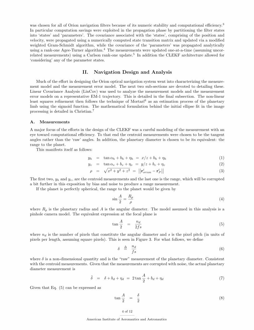
where Rp is the planetary radius and A is the angular diameter. The model assumed in this analysis is apinhole camera model. The equivalent expression at the focal plane is

tanA

2=

nd2fs

(5)

where nd is the number of pixels that constitute the angular diameter and s is the pixel pitch (in units ofpixels per length, assuming square pixels). This is seen in Figure 3. For what follows, we define

δ∆=

ndfs

(6)

where δ is a non-dimensional quantity and is the “raw” measurement of the planetary diameter. Consistentwith the centroid measurements. Given that the measurements are corrupted with noise, the actual planetarydiameter measurement is

δ̃ = δ + bd + ηd = 2 tanA

2+ bd + ηd (7)

Given that Eq. (5) can be expressed as

tanA

2=

δ

2(8)

4 of 12

American Institute of Aeronautics and Astronautics

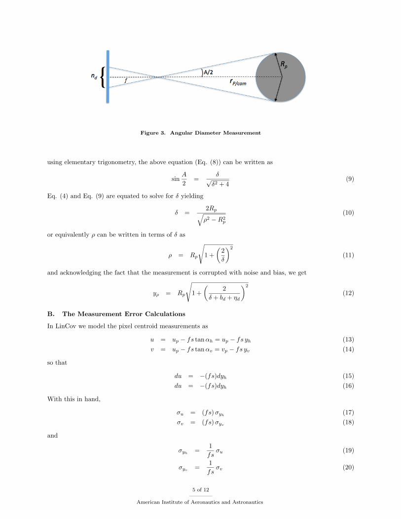
Figure 3. Angular Diameter Measurement

using elementary trigonometry, the above equation (Eq. (8)) can be written as

sinA

2=

δ√δ2 + 4

(9)

Eq. (4) and Eq. (9) are equated to solve for δ yielding

δ =2Rp√ρ2 −R2

p

(10)

or equivalently ρ can be written in terms of δ as

ρ = Rp

√1 +

(2

δ

)2

(11)

and acknowledging the fact that the measurement is corrupted with noise and bias, we get

yρ = Rp

√1 +

(2

δ + bd + ηd

)2

(12)

B. The Measurement Error Calculations

In LinCov we model the pixel centroid measurements as

u = up − fs tanαh = up − fs yh (13)

v = up − fs tanαv = vp − fs yv (14)

so that

du = −(fs)dyh (15)

du = −(fs)dyh (16)

With this in hand,

σu = (fs)σyh (17)

σv = (fs)σyv (18)

and

σyh =1

fsσu (19)

σyv =1

fsσv (20)

5 of 12

American Institute of Aeronautics and Astronautics

We have been assuming in LinCov that the pixel pitch is 4.8× 10−6 m/pixel and the focal length is 35.1 mmso that

1

fs= 1.3675× 10−4 pixels−1 (21)

which is equivalent to 28.2 arc-seconds per pixel ( = 1.3675× 10−4 · 3600 · 180/π)Given that

δ =ndfs

(22)

the error in these are found to be

dδ =1

fsdnd (23)

and

dρ = −ρ2 −R2

p

ρ

dδ

δ= −

ρ2 −R2p

ρ

dndnd

(24)

The standard deviation can be approximated as

σρ =ρ2 −R2

p

ρ

1

ndσnd

(25)

which for ρ >> Rp becomes

σρ =ρ

ndσnd

(26)

This is the error for a ‘smooth’ Moon. Terrain effects add additional error which diminishes as the rangeincreases as

σρ =

√σ2rsmooth

+ (σrterrain(ρ))2

(27)

The measurement errors are described in Christian.8 The errors associated with lunar tracking aregreatly influenced by the lunar terrain. In particular, the errors are tied to the portion of the Moon beingobserved. Since there are a limited number of lunar images available which have usable time-tags, attitudeof the camera and truth data available, computer generated images using Engineering DOUG Graphics forExploration (EDGE) were used. EDGE simulates the lunar terrain using the latest Lunar ReconnaissanceOrbiter (LRO) topography and imagery and is particularly useful because the lighting and distance can bevaried. EDGE was also used to generate Earth imagery with improved atmospheric models. A representativeEM-1 trajectory was used to generate EDGE (Earth and Moon) images to vary the lighting conditions atdifferent points in the trajectory as well as to investigate the effects of looking at different portions of theMoon. This was then used to obtain the following Moon noise error models:

σr =

√(0.12 pix)2 +

(7291.7 pix)(6562 ft)

ρ

)2

(28)

where ρ is the distance in feet and σr is the resulting radius error in pixels. The centroid angles are dependenton the illumination direction. Hence, centroid errors parallel and perpendicular to the Moon-Sun direction(α and β, respectively) were developed, once again using EDGE imagery, and are as follows:

σα =

√(0.15 pix)2 +

(7291.7 pix)(6562 ft)

ρ

)2

(29)

σβ =

√(0.06 pix)2 +

(7291.7 pix)(6562 ft)

2ρ

)2

(30)

6 of 12

American Institute of Aeronautics and Astronautics

The factor 6562 ft has to do with the expected lunar terrain variation across the lunar surface of 2 km.The bias for Moon imagery was generated by looking only at one side of the Moon and is:

bα = (0.383 pix)− 3.470× 108 pix− ft

ρ(31)

bβ = 0 (32)

br = (−0.236 pix)− 1.964× 108 pix− ft

ρ(33)

For Earth imagery the noise in analyzing EDGE imagery was found to be

σα ≈ 0.065 pix (34)

σβ ≈ 0.025 pix (35)

σr ≈ 0.058 pix (36)

(37)

with a bias on the radius measurement to be

br = (−0.263 pix)− 1.901× 108 pix− ft

ρ(38)

Obviously this is a function of the expected atmosphere ‘bias’ (in the case above the atmospher bias wastaken to be 35 km) and a the sensitivity to this has been performed.

C. LinCov Results

The Linear Covariance results are (obviously) highly dependent on the measurement and measurement errormodels used. To that end, in keeping with the design of the flight software, the environment measurementmodel was for the Moon was taken as described above. For Earth-measurement passes, the noise modelswere taken to be the same as the Moon because they were more conservative than the EDGE-generatedEarth imagery provided.

The filter (FSW) measurement error models were taken to be a constant and measurement passes veryclose to the Moon were not performed because of the large bias errors (due to lunar terrain) and the FOV ofthe camera. Analysis performed to date shows a delivery that satisfies an allowable entry corridor as shownin Figure 4.

III. Hardware and Software Tests

One of the main difficulties in testing and verification of the OpNav system is the lack of on-orbit imagerywith high-fidelity metadata as a truth source. A combination of hardware characterization, live-sky testing,and synthetic imagery were therefore used to test the system.

A. Camera Calibration and Focus

The Orion EM-1 flight camera was calibrated at the Johnson (JSC) electro-optics lab as seen in Figure 6. Thecamera requires extrinsic calibration prior to the flight for the default load of the lens distortion parameters.Additionally, we needed to permanently stake the focal length of the lens to just under infinity. This keepsthe focus from shifting during ascent vibration. Slightly focusing under infinity allows spread of the energyacross multiple pixels for sub-pixel resolution. A flat field and modulation transfer function evaluation werealso accomplished as part of the exercise as well.

All camera lenses add radial distortion to an image and sensor misalignment will add tangential distortion.Without accounting for these distortions, optical navigation measurements will yield inaccurate results.These distortions are mapped and eliminated by warping the image in the opposite direction of the distortionbefore using them for centroiding and limb finding. This process is called calibration.

The calibration was carried out using a two-axis gimbal and large collimator to account for cameradistortions due to lenses and sensor misalignment. This is completed by fastening the camera to a rotation

7 of 12

American Institute of Aeronautics and Astronautics

Figure 4. Orion Entry Interface Delivery Dispersions vs. Corridor Requirement

stage on the gimbal and panning along the horizontal field of view of 19.5 deg and a vertical field of viewof 15.6 deg in increments of 2 deg. The camera captures a total of 99 images which are then combined tomake a single composite star grid. The camera exposure was set within 1-5 ms range to avoid saturation ofpixels from the collimated light source used.

This star map is then used to create a distortion contour plot as show in Figure 5. A pinhole cameramodel was used to generate these plots and associated software, characterized by the error shown in equation39.

x′ = −tan(α)fl

dx

y′ = −tan(β)fl

dy(39)

Error =√

(x− x′)2 + (y − y′)2

where α, β are the skew angles, fl is the focal length of 43.3mm, and dx, dy are the vertical and horizontalpixel pitch of 0.018 mm/pixel. To permanently stake the focal length of the camera a 500 mm focal lengthrefractive collimator was used. This device has an objective diameter of 50mm with a 15-micron pinholereticle light source to simulate a single star. The camera and equipment or mounted on a steady base opticaltable on a steady floor and a computer is used to control the camera. Using a calibrated torque wrench thefocus is adjusted using the lens focus lock screw while using the software and collimator to locate the starwithin the center of the camera area and focus it to infinity and no pixel is saturated. This process takesseveral iterations and a final slight defocus is accomplished before tightening and staking with a stakingcompound to hold the lens in place permanently.

8 of 12

American Institute of Aeronautics and Astronautics

Figure 5. Pinhole Camera Distortion Model

Figure 6. Orion EM-1 Optical Navigation Camera Calibration (Photo courtesy NASA/Mike Ruiz)

B. Live Sky Test

Two Engineering Design Unit (EDU) cameras and an EDU star tracker were used for a live-sky test inDenver, as shown in Figure 7. The star tracker was used as a truth attitude reference in taking simulatedcalibrations and measurements from the EDU cameras. Both starfield and moon images were taken for thepurposes of calibration and taking measurements, respectively. The test provides valuable live-sky imagery,since synthetic imagery always has inherent limitations when modeling real-world effects. As mentionedbefore, in-space imagery with high-fidelity truth metadata is rare so these live-sky tests provide one of theclosest real-world analogs to operational use.

The test was performed on a clear night at a temperature between 0 and 30 degrees C with a relativehumidity of less than 65%. The Star tracker and Optical Cameras were mounted on a rigid 8 inch (203.2mm) by 10 inch (254 mm) anodized aluminum plate that was oriented and aligned using a standard magneticcompass and compensated for local magnetic declination. One of the cameras was mounted on an angledplate that could be adjusted in order to track the moon in its field of view while the Star Tracker and otheroptical camera stayed static. Several sets of images along with the metadata needed from the Star Trackerwere collected to test the optical navigation algorithms and help model real effects for simulations testingand certification.

9 of 12

American Institute of Aeronautics and Astronautics

Figure 7. The EDU camera and star tracker rig are set up for a live-sky test in Denver (Photo courtesyNASA/Steve Lockhart)

C. Hardware-in-the-Loop Lab Test

In support of systems-level verification, a hardware-in-the-loop test rig was developed in the Johnson SpaceCenter Electro-Optics Lab to exercise the OpNav system prior to integrated testing on the Orion vehicle.Figure 8 shows the rig, which the test team has dubbed OCILOT (Orion Camera In the Loop OpticalTestbed). The rig consists of an EDU opnav camera, a collimating lens, and a dense pixel display allmounted on an optical bench and micro-alignment brackets. The formal hardware-in-the-loop verificationrig uses an 8K display and an additional field flattening lens. The hardware test allows for integrated testof all the data flow, hardware connections, and real avionics.

D. Software Verification Testing

The software is primarily verified with synthetic imagery for which definitive truth data is available. Thesimulated camera field of view is shown in Figure 9. The images are generated using EDGE, which wasspecifically upgraded to include high-fidelity lunar terrain, Earth atmospheric scattering, and stellar aberra-tion which effects measurements and calibration respectively. The nominal conceptual flight profile is usedto verify performance metrics. Several hundred off-nominal images are also used to analyze robustness andfault detection in the software. These include effects such as stray light, excess radiation damage, specularreflections, etc. An example of the verification images is shown in Figure 10, where images of the Earth andMoon are tested. Of note is the stressing case in Figure D, where the crescent is quite thin. These tests alsohelp verify the tuning parameters chosen for the algorithm such as earth atmosphere bias, minimum pixelintensity, and star detection thresholds.

Acknowledgments

The authors would like to thank the outstanding team at Johnson Space Center for their contributions togetting us where we are today, with particular gratitude to Lorraine Prokop and Steven Lockhart. Addition-ally, the support of contractor partners at Lockheed Martin Space Systems was very appreciated. Finally,we would also like to acknowledge the assistance of professors John Christian, Daneila Mortari, and RenatoZanetti in algorithm research.

10 of 12

American Institute of Aeronautics and Astronautics

Figure 8. Orion Camera In the Loop Optical Testbed (Photo courtesy NASA/Steve Lockhart)

Figure 9. Simulated opnav camera field of view capturing moon image

(a) Earth Image (b) Moon Image (c) Stressing Moon Image

Figure 10. Synthetic Imagery Used for verification

11 of 12

American Institute of Aeronautics and Astronautics

References

1Battin, Richard H., “An Introduction to the Mathematics and Methods of Astrodynamics”, AIAA Education Series,Revised Edition, 1999.

2Christian, John A., Benhacine, L., and Hikes, J. et al., “Geometric Calibration of the Orion Optical Navigation CameraUsing Star Field Images, The Journal of the Astronautical Sciences, Vol. 63, No. 4, Dec. 2016.

3Bierman, G. J., Factorization Methods for Discrete Sequential Estimation, New York: Dover Publications, 2006.4Agee, W.S. and Turner, R.H., “Triangular Decomposition of a Positive Definite Matrix Plus a Symmetric Dyad with

Application to Kalman Filtering, White Sands Missile Range Tech. Rep. No. 38, 1972.5Carlson, N.A., “Fast Triangular Factorization of the Square Root Filter”, AIAA Journal, Vol. 11, No. 9, September 1973.6Mortari, Daniele, C. N. D’Souza, and R. Zanetti, “Image Processing of Illuminated Ellipsoid”, Journal of Spacecraft and

Rockets, Vol. 53, No. 3, May-June 2016.7Christian, John A., “Optical Navigation Using Planet’s Centroid and Apparent Diameter in Image”, AIAA Journal of

Guidance, Control, and Dynamics, Vol. 38, No. 2, Feb 2015.8Christian, John A., “Error Model for OPNAV Centroid and Radius Measurements”, Technical Memorandum, RPI/SEAL-

17-001, Rensselaer Polytechnic Institute, October 2017.

12 of 12

American Institute of Aeronautics and Astronautics