ORDINATIONS OF HABITAT RELATIONSHIPS AMONG BREEDING …

ORDINATIONS OF HABITAT RELATIONSHIPS AMONG BREEDING BIRDS

FRANCES C. JAMES

I N an attempt to express habitat relationships in a new way, I have applied

two methods of multivariate analysis to a large set of data pertaining to

the habitats of 46 species of common breeding birds. The question asked

was : How do these species distribute themselves with respect to the struc-

ture of the vegetation? This required (1) devising field techniques that

would give quantitative measurements of the vegetation within the breeding

territories of individual birds, (2) analyzing these by species in order to

obtain a sample of the characteristic habitat dimensions of the species niche,

(3) reconstructing the relationships among the species according to their

relative habitat separation, and (4) considering the ability of the vegetational

variables to describe differences among habitats mathematically.

Data were gathered in the spring and summer of 1967 in Arkansas. The

vegetation was sampled in O.l-acre circular plots, using singing male birds as

the centers of the circles. The statistical procedures used which were principal

component analysis and discriminant function analysis provided a tool for

describing bird distribution objectively as ordinations of continuously-varying

phenomena along gradients of vegetational structure. The relative positions

of the species were located within multidimensional “habitat space.” The

relationship between this approach and studies involving ordinations of plant

and animal communities is discussed.

FIELD METHODS

Estimates of the characteristics of the structure of the vegetation were obtained by means of sampling one 0.1~acre circular plot within the territory of each singing male bird. A 0.1.acre is a large enough area (radius 37 feet) that it should include an adequate sample of the vegetation. It is convenient to have a circular plot with its center at a singing perch selected by a territorial bird. This might give a biased view of habitat for species which occur in open areas and choose singing perches in places very different from their foraging areas, but this objection is minimized in the forest (including most of the species considered here).

The sampling technique was a modification of the range-finder circle method recom- mended by Lindsey, Barton, and Miles (1958) as a very accurate and efficient procedure. The range-finder itself was found to he unnecessary. Instead, I suspended a brightly colored yardstick at or below the spot where a territorial male bird was singing. This was sighted by holding at armslength a second yardstick having a mark equal to the length of the first when viewed from the perimeter of the circle. This proved to be an accurate and efficient way of determining whether I was within the area to be sampled. A total of 4Ql 0.1.acre circles was measured in the territories of 46 species. No attempt was made to remain within a fairly uniform stand. In fact as many habitat types as

215

216 THE WILSON BULLETIN September 1971 Vol. 33, No. 3

TABLE 1 FIFTEEN VARIABLES OF THE STRUCTURE OF THE VECETATI~N CONSIDERED IN THE ANALYSIS

OF 0.1.ACRE PLOTS SHOWING THE CORRESPONDING SYMBOLS USED IN TABLES 2 AND 3

1 %GC

2 S/4

3 SPT

4 ‘b cc

5 CH

6 TM

7 TM?

8 TM

9 TIg-15

10 T,,;

11 CH x S

12 CH x Tz--8

13

14

15

CH x T,,

T2%8

TZ>,

Per cent ground cover divided by 10

Number of shrub or tree stems less than 3 inches DBH per

two armslength transects (0.02 acres) divided by 4

Number of species of trees

Per cent canopy cover divided by 10

Canopy height divided by 10

Number of trees 3 to 6 inches DBH




Number of trees greater than 15 inches DBH

Canopy height x shrubs (variable 2 X variable 5)

Canopy height x trees 3 to 9 inches DBH [variable 5 X vari-

ables (6 + 7) 1

Canopy height x trees greater than 9 inches DBH [variable

5 X variables (8 + 9 + 10) 1

Number of trees 3 to 9 inches DBH squared [square of vari-

ables (6 + 7)1

Number of trees greater than 9 inches DBH squared [square

of variables (8 + 9 + 10) 1

possible were sampled. Data were obtained in eighteen different counties in various

parts of Arkansas. In the few cases in which two species were singing in the same 0.1.

acre circle, data for that circle were used to describe one observation of each of the

species. In the subsequent analysis data from the circles were organized by species of

bird, regardiess of where the data were obtained.

Each tree greater than three inches in diameter at breast height (DBH) within the

circle was identified to species and the size class was recorded. The same sighting

stick mentioned above was graded on the other side for three-inch size-class estimates

of tree diameters. Calibrations on the stick were determined by using the formula

S = \i(aD’) /(a + D), where S is the graduation on the stick, a is the armlength of

the observer, and D is the diameter at breast height (Forbes, 1955).

To estimate shrub density, two armlength transects together totalling 0.02 acres were

made across the circle and the number of stems intersected that were less than three

inches DHB was recorded. An estimate of ground cover was made by taking 20 plus-

or-minus readings for the presence or absence of green vegetation sighted through a

Francis C. James

HABITAT ORDINATION 21.7

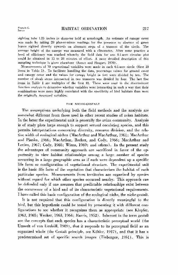
sighting tube 1.25 inches in diameter held at armslength. An estimate of canopy cover

was made by taking 20 plus-or-minus readings for the presence or absence of green

leaves sighted directly upwards on alternate steps of a transect of the circle. The

average height of the canopy was measured with a clinometer. After some practice a

level of efficiency was reached whereby the field data for one 0.1.acre circular plot

could be obtained in 15 to 20 minutes of effort. A more detailed description of this

sampling technique is given elsewhere (James and Shugart, 1970).

Measurements of 10 vegetational variables were made in each 0.1.acre circle (first 10

items in Table 1). To facilitate handling the data, percentage values for ground cover

and canopy cover and the values for canopy height in feet were divided by ten. The

number cf shrub stems intersected in two transects was divided by four. The last five

items in Table 1 are multiples of the first 10. These were used in the discriminant

function analysis to determine whether variables were interacting in such a way that their

combinations were more highly correlated with the specificity of bird habitats than were

the originally measured variables.

THE NICHE-GESTALT

The assumptions underlying both the field methods and the analysis are

somewhat different from those used in other recent studies of avian habitats.

In the latter the experimental unit is generally the avian community. Analysis

is of study plots large enough to support several coexisting species, and this

permits interpretations concerning diversity, resource division, and the rela-

tive width of ecological niches (MacArthur and MacArthur, 1961; MacArthur

and Pianka, 1966; MacArthur, Recher, and Cody, 1966; MacArthur and

Levins, 1967; Cody, 1968; Wiens, 1969; and others). In the present study

the advantages of community approach are sacrificed in favor of the op-

portunity to view habitat relationships among a large number of species

occurring in a large geographic area as if each were dependent up a specific

life form or configuration of vegetational structure. The experimental unit

is the basic life form of the vegetation that characterizes the habitat of each

particular species. Measurements from territories are organized by species

without regard for which other species occurred nearby. This approach can

be defended only if one assumes that predictable relationships exist between

the occurrence of a bird and of its characteristic vegetational requirements.

I have called this basic configuration of the ecological niche, the niche-gest&

It is not required that this configuration is directly meaningful to the

bird, but this hypothesis could be tested by presenting it with different con-

figurations to see whether it recognizes them as appropriate (see Klopfer,

1963, 1965; Wecker, 1963, 1964; Harris, 1952). Inherent in the term gestalt

are the concepts that each species has a characteristic perceptual world (the

Umwelt of von Uexkiill, 1909), that it responds to its perceptual field as an

organized whole (the Gestalt principle, see Kohler, 1947)) and that it has a

predetermined set of specific search images (Tinbergen, 1951). This is

218 THE WILSON BULLETIN September 19il V”l. 83, No. 3

BELL’ S VIREO

WARBLING VIREO WHITE- EYE0 VIREO

YELLOW-THROATED VIREO RED-EYED VIREO

FIG. 1. Outline drawings of the niche-gestalt for five species of vireos, representing the visual configuration of those elements of the structure of the vegetation that were consistently present in the habitat of each. Numbers give the vertical scale in feet.

Francis C. HABITAT ORDINATION 219 .lanEs

YELLOWTHROAT

HOODED WARBLER

PARULA WARBLER

REDSTART

BLACK-AND-WHITE WARBLER

OVENBIRD

FIG. 2. Outline drawings of the niche-gestalt for six species of warblers, representing the visual configuration of those elements of the structure of the vegetation that were consistently present in the habitat of each. Numbers give the vertical scale in feet.

220 THE WILSON BULLETIN

FIG. 3. Marsh at the edge of Lake Sequoyah, five miles east of Fayetteville, Wash- ington Co., Ark., where Bell’s Vireos and Yellowthroats had breeding territories.

assumed to be at least partially genetically determined, but is surely also

modifiable by experience and subject to ecological shift under varying cir-

cumstances. Whereas the community approach is sensitive to shifts in habitat

due to such factors as competition for resources, the present approach is an

attempt to define relationships among birds based upon the basic life forms

of the vegetation which each species requires. Since the geographic range

of every species is unique and since species are uniquely adapted to utilize

certain aspects of their environment, I hope the reader will agree that this

approach is justified.

The outline drawings (Figs. 1 and 2) are examples of visual descriptions

of the life forms of the vegetation that were consistently present in the

habitats of the species in question. These were made by comparing notes

and photographs of each O.l-acre circle where a species occurred and by

selecting only the features in common. Conversely, if definable niche-gestalt

units occur, it should be possible to discover as many of these units as there

are pairs of breeding birds in any one place. For example the vegetational

configuration in the drawings for the Bell’s Vireo (Fig. 1) and the Yellow-

throat (Fig. 2) can be identified in a photograph of a place where both

occurred (Fig. 3). Likewise the configurations which characterize the habi-

HABITAT ORDINATION

FIG. 4. Vegetation along the Mulberry River, five miles east of Cass, Franklin Co..

Ark., where pairs of White-eyed Vireos, Redstarts, and Parula Warblers were nesting.

tats of the White-eyed Vireo (Fig. I ), American Redstart, and Parula

Warbler (Fig. 2) can be identified in Figure 4; a territorial male Red-eyed

Vireo (Fig. 1 j, Hooded Warbler, and Ovenbird (Fig. 2) were each present

where Figure 5 was photographed.

An attempt will be made to reconstruct relationships between species-

specific niche-gestalt units from the quantitative data and to view them in

multidimensional “habitat space.” Of course this space also contains gra-

dients in types of food, nest-sites, microclimate, etc. Although these variables

are undefined in the present study, they would have to be included in a

thorough analysis of the ecology of adaptation.

RESULTS

Correlations Among Vegetational Variables.-The vegetational variables

are highly interrelated. In the correlation matrix (Table 2) all values of r

greater than 0.39 are significant at (Y = 0.01 (44 df). The first column.

percentage of ground cover, is negatively correlated with all of the other

variables. The second column, an estimate of shrub density, has a different

pattern of variation from the last eight columns, which are all characteristics

of trees. Shrub density varies concordantly with the number of small trees

222 THE WILSON BULLETIN September 1971 Vol. 83, No. 3

FIG. 5. Upland mesic forest at Cherry Bend, Franklin Co., Ark., in the Ozark National Forest, where Red-eyed Vireos, Ovenbirds, and Hooded Warblers had breeding territories.

and also with the number of species of trees and canopy cover. But shrub density varies independently of canopy height and trees greater than six

inches DBH. Correlations between the number of species of trees per unit

area, percentage of canopy cover and canopy height are particularly highly re-

lated to each other and to tree density by size classes (last five columns).

This means that for a 10 X 46 data matrix of mean values of each vegeta-

tional variable for each species (see next section), a large amount of the

variation is statistically attributable to these variables. Although there ap-

pears to be redundancy in the five interrelated variables for number of trees

by size classes (last five items in Table 2), it will be shown in a later section

that each contributes significantly to the statistical description of habitat

differences among the species of birds.

PRINCIPAL COMPONENT ANALYSIS

Morrison (1967) defines principal components as those linear combina-

tions of the responses which explain progressively smaller portions of the

total sample variance. The components can be interpreted geometrically as

the variates corresponding to the principal axes of the scatter of observations

in space. If a sample of N trivariate observations had the ellipsoidal scatter

HABITAT ORDINATION 223

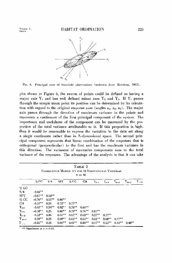
FIG. 6. Principal axes of trivariate observations (redrawn from Morrison, 1967).

plot shown in Figure 6, the swarm of points could he defined as having a

major axis Y, and less well defined minor axes Yp and Ys. If Y1 passes

through the sample mean point its position can he determined by its orienta-

tion with regard to the original response axes (angles al, a2, a3). The major

axis passes through the direction of maximum variance in the points and

represents a continuum of the first principal component of the system. The

importance and usefulness of the component can be measured by the pro-

portion of the total variance attributable to it. If this proportion is high,

then it would be reasonable to express the variation in the data set along

a single continuum rather than in N-dimensional space. The second prin-

cipal component represents that linear combination of the responses that is

orthogonal (perpendicular) to the first and has the maximum variance in

this direction. The variances of successive components sum to the total

variance of the responses. The advantage of the analysis is that it can take

TABLE 2

CORRELATION MATRIX (r) FOR 10 VEGETATIONAL VARIABLES

N = 46

%GC S/4 SPT

70 CC CH T LB TbQ T

TZ

T >u

-0.44* * -0.67* * -0.76** -0.51** -0.63** -0.W * -0.52*’ -0.5g** -0 45**

0.54** 0.55** 0.80** 0.23 0.72** 0.77** 0.54** 0.92** 0.76** 0.60** 0.25 0.80** 0.79** 0.76’* 0.81** 0.06 0.61** 0.61** 0.63** 0.57** 0.77** 0.15 0.69** 0.63** 0.65** 0.61** 0.68** 0.77** 0.16 0.66** 0.62** 0.81** 0.47** 0.55** 0.43** 0.48**

** Significant at (Y = 0.01.

THE WILSON BULLETIN September 1971 Vol. 83, No. 3

TABLE 3

SUMMARY OF THE RESULTS OF THE PRINCIPAL COMPONENT ANALYSIS OF MEAN VALUES

OF EACH OF 10 VEGETATIONAL VARIARLES FOR 46 SPECIES OF BREEDING BIRDS

I

component

II III IV

Percentage of total variance accounted for Cumulative percentage of total variance accounted for Correlations to original variables

%‘.X

s/4 SPT

%CC CH TS-II T TZ T,1, T > I.5

64.8 12.5 7.7 4.9

64.8 77.3 85.0 89.9

-0.77 0.21 0.15 0.53 0.46 -0.83 0.04 0.03 0.93 -0.16 0.03 0.17 0.91 -0.17 0.06 -0.12 0.84 0.25 0.35 0.01 0.87 -0.25 -0.14 0.29 0.89 0.16 -0.12 0.25 0.76 0.41 -0.34 0.01 0.80 0.30 -0.27 -0.13 0.71 0.22 0.62 -0.07

N-dimensional data and reduce it to a few new variables which account for

known amounts of the variation in the original set.

In the present case, the basic ten vegetational variables (first 10 items in

Table 1) are used as coordinates of a hypothetical ten-dimensional space.

Each of the 46 species of birds has a position in this space according to

the mean values of the variables for the O.l-acre circles measured. This

complex situation is analyzed so that a few new variables, the principal com-

ponents are derived. The principal component analysis is summarized in

Table 3.

The first or major component accounts for 64.8 per cent of the total vari-

ance and is highly correlated with all of the original variables. All values

are positive except percentage of ground cover. The highest correlations are

with number of species of trees per O.l-acre, percentage of canopy cover, num-

ber of small trees, and canopy height. Species found where ground cover is

high and where there are few shrubs and trees would be expected to have

low values of the first component. Species found in mature forests, where

ground cover is low and there are many trees of various species and sizes,

would be expected to have high values of this component.

The second principal component accounts for an additional 12.5 per cent

of the total variance (Table 3). C orrelations between it and the original

Francis C. James


variables show that it represents an inverse interaction between medium-sized

trees and shrub density. Species inhabiting dense shrubs would have low

values of this component. Species found where there are medium-sized trees

and few shrubs would have high values of the second component. The third

component accounts for 7.7 per cent of the variance in addition to that al-

ready explained. It represents parkland, the presence of large trees with the

absence of smaller ones. The fourth component, representing 4.9 per cent

of the variance is most closely associated with ground cover. By means of

these four newly-computed variables, it has been possible to account for 89.9

per cent of the variation in the original data set. The analysis has derived

a parsimonious description of the dependence structure of the multivariate

system.

Now it is possible to reconstruct the habitat relationships among these

species using the components as coordinates. Figure 7 is a three-dimensional

view of the position of each species listed in Table 4 along the axes of the

first three principal components. The horizontal axis, representing the first

component, has separated the species fairly regularly from open-country

birds on the left found in places having high ground cover and few trees

(Prairie Warbler, Bell’s Vireo, Yellow-breasted Chat, Brown Thrasher) to

birds on the right found in well-developed shaded forests (Ovenbird, Red-

eyed Vireo, Wood Thrush). In the center along this axis falls a group of

species that show remarkable latitude in their choice of habitat (Cardinal,

Brown-headed Cowbird, Blue-gray Gnatcatcher). The axis of the second

principal component extends backwards from species found in shrubs and

low trees (Catbird, White-eyed Vireo, Kentucky Warbler) in the foreground

toward species found where there is limited understory (Prothonotary War-

bler, Robin, Red-headed Woodpecker). The axis of the third component

extends vertically from species not dependent on large trees to those re-

quiring large trees. The highest circles are for the Baltimore Oriole and

Hooded Warbler.

Distances between species in Figure 7 represent ecological differences in

“habitat space.” Consider the positions of the five species of vireos. Their

major separation is accomplished along the axis of the first principal com-

ponent in the order Bell’s, Warbling, White-eyed, Yellow-throated, and Red-

eyed. This ordering corresponds to increases in the following: number of species of trees per unit area, percentage of canopy cover, number of small trees

per unit area, and canopy height (see legend for Fig. 7). Along the axis of

the second component (bases of the vertical lines) the same species fall in

the order White-eyed, Red-eyed, Bell’s, Warbling, and Yellow-throated. This

axis is defined as increasing number of medium-sized trees and/or decreasing

shrub density. Along the axis of the third component (height of circles) the

Francis C. James


TABLE 4

LIST OF SPECIES IN ALPHABETICAL ORDER GIVING SYMBOLS USED IN FIGURES 7 AND 9

AF BG B-GG B-HC

BJ BO BT BV BWW C CB cc CF CG cs cw DW EK FS HW IB KW LW 0 00 PW PAW PRW RS RO R-BW R-EV R-HW R-ST SCT SUT TT W-BN W-EV WP WT WV Y Y-BCH Y-BCU Y-TV

Acadian Flycatcher Blue Grosbeak Blue-gray Gnatcatcher Brown-headed Cowbird Blue Jay Baltimore Oriole Brown Thrasher Bell’s Vireo Black-and-White Warbler Cardinal Catbird Carolina Chickadee Crested Flycatcher Common Grackle Chipping Sparrow Carolina Wren Downy Woodpecker Eastern Kingbird Field Sparrow Hooded Warbler Indigo Bunting Kentucky Warbler Louisiana Waterthrush Ovenbird Orchard Oriole Prairie Warbler Parula Warbler Prothonotary Warbler American Redstart Robin Red-bellied Woodpecker Red-eyed Vireo Red-headed Woodpecker Rufous-sided Towhee Scarlet Tanager Summer Tanager Tufted Titmouse White-breasted Nuthatch White-eyed Vireo Eastern Wood Peewee Wood Thrush Warbling Vireo Yellowthroat Yellow-breasted Chat Yellow-billed Cuckoo Yellow-throated Vireo

(Empidonax virescens)

(Guiraca caerulea)

(Polioptila caerulea)

(Molothrus ater)

(Cyanocitta cristata)

(Icterus galbula)

(Toxostoma rufum)

(Vireo bellii)

(Mniotilta varia)

(Richmondena cardinalis)

(Dumetella carolinensis)

(Parus carolinensis)

(Myiarchus crinitus)

(Quiscalus quiscula)

(Spizella passerina)

(Thryothorus ludovicianus)

(Dendrocopos pubescens)

(Tyrannus tyrannus)

(Spizella pusilla)

( Wilsonia citrina)

(Passerina cyanea)

(Oporornis jormosus)

(Seiurus motacilla)

(Seiurus aurocapillus)

(Icterus spurius)

(Dendroica discolor)

(Parula americana)

(Protonotaria citrea)

(Setophaga ruticilla)

(Turdus migratorius)

(Centurus carolinus)

(Vireo olivaceus) (Melanerpes erythrocephalus)

(Pipilo erythrophthalmus)

(Piranga olivacea) (Piranga rubra)

(Parus bicolor)

(Sitta carolinensis)

(Vireo griseus)

(Contopus virens)

(Hylocichla mustelina)

(Vireo gilvus)

iGeothlypis t&has)

(Icteria virens)

(Coccyzus americanus)

C Vireo flavifrons)

THE WILSON BULLETIN September 1971 Vol. 83, No. 3

TABLE 5

RESIJLTS OF THE DISCRIMINANT FUNCTION ANALYSIS AND STEP-DOWN PROCEDURE -

The computed coefficients (w) for the formula D = Z WI 21, and the ranking of the vegetational variables (x) are given in the order of their respective power to separate the species of birds by habitat. Each variable had a significant ability to separate the species in addition to that separation already achieved by all the variables above it on the list.

Original Computed order of weight

Rank VUid& Verretational variable ( x 1 (w) F-ratio*

1 4 2 r 3 : 4 12 5 13 B 2 7 11 8 6 9 1

10 14 11 7 12 9 13 8 14 10 15 15

Percentage canopy cover Canopy height Number of species of trees Canopy height x trees 3-9 inches DBH Canopy height x trees larger than 9 inches DBH Shrub sterns/0..2-acre Canopy height X shrubs Trees 3-6 inches DBH Percentage ground cover Trees 3-9 inches DBH squared Trees 6-9 inches DBH Trees 12-15 inches DBH Trees 9-12 inches DBH Trees larger than 15 inches DBH Trees larger than 9 inches DBH squared

2.0197 46.05 1.5305 16.58 0.5807 9.76

-0.0954 4.73 0.0803 5.23 0.3091 11.28

-0.0131 6.51 1.1134 5.47

-0.2861 7.24 0.0117 5.01

-0.2592 4.80 2.2260 4.88 2.8539 4.37 2.9848 5.87

-0.2284 6.39

* All F-ratios are significant at IY = .OOl.

Warbling and Yellow-throated Vireos have higher positions than the others,

indicating that they require the presence of higher trees. These relationships

can be checked by considering the drawings in Figure 1 in the order that

the species fall along the respective axes. The same procedure can be ap-

plied to the six species of warblers for which the niche-gestalt is outlined in

Figure 2.

Although the species in Figure 7 are fairly evenly distributed, several

appear to be more isolated than the others, and these are birds that are not

widely distributed in Arkansas in the breeding season. The Baltimore Oriole

occurs in summer only in places having very large trees with clearings

below. These are in towns and farmyards in the southern parts of the

state and along river banks. Warbling Vireos are confined to cottonwoods

(Populus) and willows (S&x) along major rivers or adjacent to them. Hooded

Warblers occur in upland and lowland situations but only in the most mature

mesic forests. I do not want to exaggerate the validity of specific relationships. This


analysis is based on mean values of the vegetational variables without regard

for their variance. Sample sizes by species are small, and data pertain to

a limited area of the breeding range of each. Nevertheless, a complex en-

vironmental situation has been reduced to a manageable mathematical and

diagrammatic structure.

DISCRIMINANT FUNCTION ANALYSIS AND STEP-DOWN PROCEDURE

The entire data set, values of 15 vegetational variables (Table 1) for 401

tenth-acre circular plots representin g the habitats of 46 species of birds was

subjected to a type of multivariate technique known as Fisher’s classical

method of discriminant function analysis (Fisher, 1936; 1938). This pro-

cedure computes an equation that is constructed in such a way that it defines

a linear axis through the data set which maximizes the differences among

populations. The new axis (D) serves as a better discriminant than do any

of the variables taken singly (Sokal and Rohlf, 1969). The result is a set

of discriminant function coefficients (wr, ws, . . . , w,,) for the 15 vegetational

variables which maximizes the F-ratio of the corresponding univariate one-

way analysis of variance applied to a linear combination of the multivariate

measurements. The average value of the discriminant function for a species

can be expressed as

where each ii is the mean of the observations of that variable for that species.

For an individual bird,

D=wr(%GC) +W2@/4) +wa(SPT) . . ..wlr. (T>J2

The values w for each vegetational variable are given in Table 5.

This method provides an optimum procedure for separating the habitats

mathematically and it permits a linear ordering of the species such that their

separation on the discriminant function axis is a function of their differences

in habitat. The order should be similar to that along the first principal com-

ponent except that the species should be more evenly distributed along the

discriminant function axis. Wh ereas the principal component analysis de-

scribed the relative positions of the species in multidimensional space (each

component of which is orthogonal to every other but in which differences are

not necessarily maximized) the discriminant function analysis maximizes

the distances between species in this space. Figure 8 gives the positions of

the species along the discriminant function axis.

Here a 15-dimensional system has been reduced to one dimension, and all

the measurements are accounted for simultaneously. The result is a continuum

of vegetational structure along which the mean values of D for each species

are located. The linear discriminant function is an expression of a con-

230 THE WILSON BULLETIN

PRAIRIE WARBLER

BELL'S VIREO

BROWN THRASHER

YELLOWTHROAT

FIELD SPARROW

BLUE GROSBEAK

EASTERN KINGBIRD

YELLOW-BREASTED CHAT

CHIPPING SPARROW

RUFOUS-SIDED TOWHEE

ORCHARD ORIOLE

INDIGO BUNTING

ROBIN

COMMON GRACKLE

CARDINAL

RED-HEADED WOODPECKER

CATBIRD

KENTUCKY WARBLER

BLUE-GRAY GNATCATCHER

BROWN-HEADED COWBIRD

RED-BELLIED WOODPECKER

LOUISIANA WATERTHRUSH

BALTIMORE ORIOLE

BLUE JAY

SUMMER TANAGER

WARBLING VIREO

PROTHONOTARY WARBLER

WHITE-EYED VIREO

CAROLINA CHICKADEE

REDSTART

YELLOW-BILLED CUCKOO

CRESTED FLYCATCHER

WOOD PEWEE

SCARLET TANAGER

HOODED WARBLER

TUFTED TITMOUSE

DOWNY WOODPECKER

BLACK AND WRITE WARBLER

YELLOW-THROATED VIREO

WHITE-BREASTED NUTHATCH

PARULA WARBLER

WOOD THRUSH

OVENBIRD

CAROLINA WREN

RED-EYED VIREO

ACADIAN FLYCATCHER

September 1971 Vol. 83, No. 3

Francis C. Jam‘3


tinuum from xeric to mesic situations, from upland to bottomland, from low

to high biomass, and from open country to forest associations. Each species

of bird has a unique mode of environmental response along this continuum.

A two-dimensional separation of the species was achieved by computing

the second characteristic root from the same data (third graph in Fig. 9).

This gave new coefficients for the vegetational variables and new average

values along a second axis for each species. This second ordination (Ds)

proceeds from areas having large isolated trees with relatively open under-

story to areas having the biomass concentrated in the lower strata, i.e. high

shrubbiness or a high number of small trees. For example, the Robin re-

quires isolated trees (low value of Da) whereas the Catbird requires dense

low trees or shrubs (high value of Ds).

The power of the method to separate the species of birds is partly deter-

mined by the number of variables considered. Examples using 3, 10 and 15

variables (in the order given in Table 5) show the additional separation

that is possible as the number of variables increases (Fig. 9). Compare also

with Cody (1968).

Once it has been established that discrimination can be accomplished, i.e.

that the species of birds can be separated stochastically according to their

habitats, Bargmann’s extension (1962) can be used to find a minimal set

of variables for discrimination. The method requires an a priori ordering

of the variables, then proceeds by selecting a subset and testing the hypothesis

that the remaining variables give no additional contribution to the discrimi-

nation. This step-down procedure provided a list of the vegetational variables

in the order of their respective ability to separate the species of birds. The

computed F-ratios of Table 5 reflect the power of each variable to separate

the species in addition to that separation already achieved by all the variables

above it on the list.

Surprisingly, every one of the 15 variables considered had a significant

ability to separate the species of birds (Table 5). By far the most powerful

were the two which would probably be the most conspicuous visually, per-

centage of canopy cover and canopy height. These were followed by the

number of species of trees, a factor closely related to tree-species diversity.

Next came two variables which combined canopy height and some aspect

of tree density: canopy height times trees three to nine inches DBH, and

canopy height times trees greater than nine inches DBH. The next three

variables were related to the density of shrubs or small trees: shrub density,

f

FIG. 8. Ordination of the habitats of 46 species of birds along a linear discriminant

function.

232 THE WILSON BULLETIN September 1971 Vol. 83. No. 3

canopy height times shrub density, and trees three to six inches DBH. After

ground cover the last six variables, although still highly significant, were

probably those that are least conspicuous in the visual configuration of the

habitat. They were measurements of tree density by size class.

This does not mean that all 15 variables are required to maximally separate

any two species, but only that all are required to separate some species from

all of the others. It should also be possible to define other variables that

would give additional separation.

DISCUSSION

The value of multivariate methods to analyze sets of dependent variables

has been exploited widely in systematics under the name of numerical tax-

onomy (Sokal and Sneath, 1963). That the methods are equally useful in

ecology is suggested by several recent applications to ecological data. Ex-

amples include cluster analyses of forests (West, 1966)) the characteristics

of the life history of beetles (Fujii, 1969), and of climatic variables (Johns-

ton, 1969) ; principal component analysis of stands of vegetation (Orloci,

1966; Austin, 1968; Swan et al., 1969; and others) and of grain bulk eco-

systems (Sinha et al., 1969) ; d iscriminant function analysis of habitats of

grassland birds (Cody, 1968).

The assumptions underlying the present study are conceptually related to

the individualistic concept of distribution described by Gleason (1926) for

plant species. This was extended by workers at the University of Wisconsin

who developed the continuum concept of plant distribution and devised

mathematical procedures for its expression (Curtis and McIntosh, 1951; Bray

and Curtis, 1957; Beals, 1960; and others). These studies show that in a

series of stands any particular species has distinct conditions for optimum

development and that to consider species as organized into discrete com-

munities is to exaggerate the dependence between them.

Bond (1957) demonstrated that the continuum concept has usefulness in

analyzing bird distribution. He concluded that “the importance of the life

form and physical features of the habitat in the distribution of birds, the

occurrence of similar bird species in similar life form situations in different

biomes, the indistinctness of boundaries between units, all suggest that the

unitary nature of community categories should be questioned.” A compari-

son between the one dimensional ordination in Figure 8 extracted by dis-

criminant function analysis with the position of the same species of birds

along the plant continuum described by Bond (ibid.) shows many similarities.

Whether the differences are due to the difference between the two methods

of analysis, the difference between Wisconsin and Arkansas, or to differences

in habitat preferences of the populations is not evident.

Francis C. James

2.0

0.0

31 I.0

0.0

-2.0

-4.0

-6.0

-8.0

-10.0 II 2.0

0.0

-2.0

-6.0

-8.0

-10.0

HABITAT ORDINATION

3 .

. D . . l . . - .

.._.‘S * . . . :..

. . .* s * . . . . *.- . .

. . . .

.

.

233

Variables

L

IO Variables .PRW

-80 .R-HW

. KW

.W-E”

I I I .CB I ‘I

15 Variables

.KW

.W-E”

I I .CS I I I IO 20 30 40 501

FIG. 9. Two-dimensional ordinations of the habitats of birds representing their positions with respect to the first and second discriminant function axes. Comparisons reveal the additional separation of populations that is possible by consideration of an increasing number of variables. The variables are in the order in which they are listed in Table 5. See sections on Discriminant Function Analysis and Discussion for further explanation.

234 THE WILSON BULLETIN September 1971 Vol. 83. No. 3

Beals (1960) extended the application of the continuum concept to bird

distribution by constructing a two-dimensional ordination of 24 forest stands

based on -their avifaunal similarities. He was able to relate this environ-

mental complex to tree speeies~ distribution and vegetational structure. Re-

cently the mathematical procedure he-used has been criticized on the basis

that the method of axis construction is a falseestimate of a Euclidean measure

of distance, that the axes in multidimensional ordinations are oblique rather

than orthogonal (Austin and Orloci, 1966; Orloci, 1966) and that the axes

are not objectively selected (Swan et al., 1969). These workers agree that a principal component analysis of a matrix of weighted similarity coefficients

between species is not subject to these objections and is the best technique

presently available for ordination work.

In the present study the combination of two multivariate methods proved

to be more informative than either would have been alone. By considering

the species means as individuals and the vegetational variables as attributes,

a principal component analysis of the correlation matrix extracted four de-

finable axes which accounted for 90 per cent of the variation in the original

data set. A discriminant function analysis of 401 tenth-acre samples rep-

resenting the habitats of 46 species of birds provided ordinations in which

the species were maximally separated according to their habitat relationships.

A step-down procedure evaluated the relative power of the 15 vegetational

variables to achieve discrimination.

I would like to emphasize the point that the methods used to obtain or-

dinations are merely objective ways of viewing sets of multivariate data.

Their use does not restrict the interpretation of results to the framework of

the continuum concept. If the species had appeared as clusters in Figures 7,

S and 9, one might be justified in interpreting these as belonging to species-

groups having similar habitat types. On the other hand, the graphs in Figure

9 reveal the risk involved. The first one, made on the basis of the three

most powerful variables for separating the species (canopy cover, canopy

height, and number of species of trees per unit area), appears to have clusters

of species at each end with a gap in the middle. When additional variables

were included in the same program, the cluster on the left disappeared. The

open-country birds became spread out along the second axis, but the cluster

on the right remained. In other words, the choice and number of variables

affect the results to such an extent that caution regarding conclusions is in

order.

SUMMARY

Quantitative vegetational data obtained in the breeding territories of 46 species of birds are organized by species as samples of the characteristic life form of the vegetation for each. Examples of outline drawings of the niche-gestalt represent those structural

Francis C. James HABITAT ORDINATION 255

features of the vegetation that were ccnsistently present where a certain species occurred.

Principal components and discriminant functions are used to describe habitat relation-

ships among the species as positions along one-, two- and three-dimensional continua

representing gradients in the structure of the vegetation. Although all 15 vegetational

variables contributed significantly to the ordinations, the most powerful variables for

describing habitat differences were per cent canopy cover, canopy height, and the number

of species of trees per unit area. If one considers the vegetation of a geographic area

to be a set of continuously-varying phenomena, and if one assumes that bird distribution

is at least partly based on species-specific adaptiveness to the resources offered by this

heterogeneous structure, then ordination procedures are appropriate methods for its ex-

pression.

ACKNOWLEDGMENTS

It is a pleasure to thank my husband, Douglas A. James, and also James E. Dunn and

Richard F. Johnston for assistance with analysis. These three plus Clarence Cottam,

George M. Sutton, Edward E. Dale, Jr. and John A. Sealander read drafts of the manu-

script and made helpful suggestions. Financial assistance was received as a University

of Arkansas Computing Center Grant, a Josselyn Van Tyne Memorial Research Award

from the American Ornithologists’ Union, and from the University of Arkansas Museum.

LITERATURE CITED

AUSTIN, M. P. 1968. An ordination study of a chalk grassland community. J. Ecol.,

56 : 739-757.

AUSTIN, M. P., AND L. ORLOCI. 1966. Geometric models in ecology. 11. An evaluation

of some ordination techniques. J. Ecol., 54:217-227.

BARCMANN, R. 1962. Representative ordering and selection of variables. Cooperative

Research Project No. 1132 Final Report, U.S. Office of Education, Dept. Health,

Education and Welfare.

BEALS, E. W. 1960. Forest bird communities in the Apostle Islands of Wisconsin.

Wilson Bull., 72: 156181.

BOND, R. R. 1957. Ecological distribution of breeding birds in the upland forests of

southern Wisconsin. Ecol. Monogr., 27:351-384.

BRAY, J. R., AND J. T. CURTIS. 1957. An ordination of the upland forest communities

of southern Wisconsin. Ecol. Monogr., 27:325-349.

CODY, M. L. 1968. On the methods of resource division in grassland bird communities.

Amer. Naturalist, 102:107-147.

CURTIS, J. T., AND R. P. MCINTOSH. 1951. An upland forest continuum in the prairie-

forest border region of Wisconsin. Ecology, 32:476496.

FISHER, R. A. 1936. The use of multiple measurements in taxonomic problems. Ann.

Eugenics, 7:179-188.

FISHER, R. A. 1938. The statistical utilization of multiple measurements. Ann. Eu-

genics, 8:376-386.

FORBES, R. D. ted.). 1955. Forestry handbook. The Ronald Press Company, New

York.

FUJII, K. 1969. Numerical taxonomy of ecological characteristics and the niche con-

cept. Syst. Zool., 18:151-153.

GLEASON, H. A. 1926. The individualistic concept of plant association. Bull. Torrey

Bot. Club, 53:7-26; reprinted in Amer. Mid]. Nat., 21:922110, 1939.

236 THE WILSON BULLETIN September 19il Vol. 83, No. 3

HARRIS, V. T. 1952. An experimental study of habitat selection by prairie and forest races of the deermouse, Peromyscus maniculatus. Contrib. from the Laboratory of Vertebrate Biology, No. 56, Univ. Michigan Press, Ann Arbor.

JAMES, F. C., AND H. H. SIIUGART, JR. 1970. il quantitative method of habitat description. Audubon Field Notes, 24:727-736.

JOHNSTON, R. F. 1969. Character variation and adaptation in European sparrows. Syst. Zool., 18:20&231.

KLOPFER, P. 1963. Behavioral aspects of habitat selection: the role of early experience. Wilson Bull., 75: 15522.

KLOPFER, P. 1965. Behavioral aspects of habitat selection: a preliminary report on stereotypy in foliage preferences of birds. Wilson Bull., 77:37&381.

K~~HLER, W. 1947. Gestalt psychology. Liveright Publ. Corp., New York. LINDSEY, A. A., J. D. BARTON AND S. R. MILES. 1958. Field efficiencies of forest

sampling methods. Ecology, 39:428-444. MACARTHUR, R. H., AND R. LEVINS. 1967. The limiting similarity, convergence, and

divergence of coexisting species. Amer. Naturalist, 101:377-385. MACARTHUR, R. H., AND J. W. MACARTHUR. 1961. On bird species diversity. Ecology,

42 : 594-598. MACARTHUR, R. H., H. RECIIER, AND M. CODY. 1966. On the relation between habitat

selection and species diversity. Amer. Naturalist, 100:319-332. MACARTHUR, R., AND E. PIANKA. 1966. On optimal use of a patchy environment.

Amer. Naturalist, 100:603-609. MORRISON, D. F. 1967. Multivariate statistical methods. McGraw-Hill Book Co., New

York. ORLOCI, L. 1966. Geometric models in ecology. 1. The theory and application of some

ordination methods. J. Ecol., 54:193-215. SINIIA, R. N., H. A. H. WALLACE, AND F. S. CH~BIB. 1969. Principal-component anal-

ysis of interrelations among fungi, mites and insects in grain bulk ecosystems. Ecology, 50:536-547.

SOKAL, R. R., AND F. J. ROHLF. 1969. Biometry. W. H. Freeman and Co., San Fran- cisco.

SOKAL, R. R., AND P. H. A. SNEATH. 1963. Principles of numerical taxonomy. W. H. Freeman and Co., San Francisco.

SWAN, J. M. A., R. L. DIX, AND C. F. WEIIRHAHN. 1969. An ordination technique based on the best possible stand-defined axes and its application to vegetational analysis. Ecology, 50:206-212.

TINBERGEN, N. 1951. The study of instinct. Oxford Univ. Press, London. UEXK~LL, J. VON. 1909. Umwelt und Innenwelt der Tiere. Springer-Verlag, Berlin. WECKER, S. C. 1963. The role of early experience in habitat selection by the prairie

deermouse, Peromyscus maniculatus bairdi. Ecol. Monogr., 33:307-325. WECKER, S. C. 1964. Habitat selection. Sci. Amer., October, pp. 109-116. WEST, N. E. 1966. Matrix cluster analysis of montane forest vegetation of the Oregon

Cascades. Ecology, 47:975980. WIENS, J. A. 1969. An approach to the study of ecological relationships among grass-

land birds. Ornithol. Monogr. 8.

UNIVERSITY OF ARKANSAS MUSEUM, FAYETTEVILLE, ARKANSAS 72701, 20 JULY

1970.

ORDINATIONS OF HABITAT RELATIONSHIPS AMONG BREEDING …

Documents

Transcript of ORDINATIONS OF HABITAT RELATIONSHIPS AMONG BREEDING …