Order Picking Policies:Pick Sequencing, Batching and

Zoning

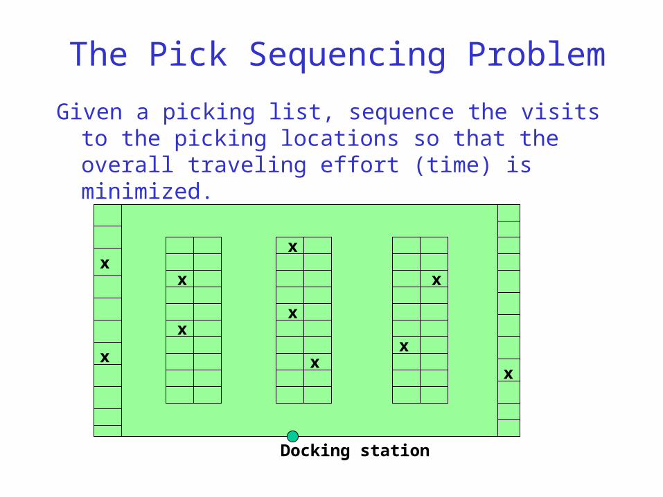
The Pick Sequencing Problem

Given a picking list, sequence the visits to the picking locations so that the overall traveling effort (time) is minimized.

x

x

x

x

x

x

x

x

x

x

Docking station

Problem Abstraction: The Traveling Salesman Problem (TSP)

Given a complete TSP graph:

1

2

3

45

c_ij

find a tour that visits all cities, with minimal total (traveling) cost; e.g.:

1

2

3

45

<1, 2, 5, 3, 4>

Analytical Problem FormulationParameters:

– N : graph size (number of graph nodes)

– c_ij : cost associated with arc (i,j)

Decision Variables:

– x_ij : binary variable indicating whether arc (i,j) is in the optimal tour

– u_i : auxiliary (real) variable for the formulation of the “no subtour” constraints

min _i _j c_ij x_ij

s.t.

_j x_ij = 1 i

_i x_ij = 1 j

(No subtours:

u_i - u_j + N x_ij N-1 i,j {2,…,N} and ij )

x_ij {0, 1} i,j

Some remarks on the TSP problem and its application in pick sequencing

• The TSP problem is an NP-complete problem: It can be solved optimally for small instances, but in general, it will be solved through heuristics.

• There is a vast literature on TSP and the development of heuristic algorithms for it (e.g., Lawler, Lenstra, Rinnooy Kan and Shmoys, “The Traveling Salesman Problem: A guided tour of combinatorial optimization”, John Wiley and Sons, 1985).

• When the “no subtour” constraint is removed, the remaining formulation defines a Linear Assignment Problem (LAP) (which is an easy one; e.g., the “Hungarian Algorithm”) => Solving the corresponding LAP can provide lower bounds for assessing the sub-optimality of the solutions provided by the applied heuristics.

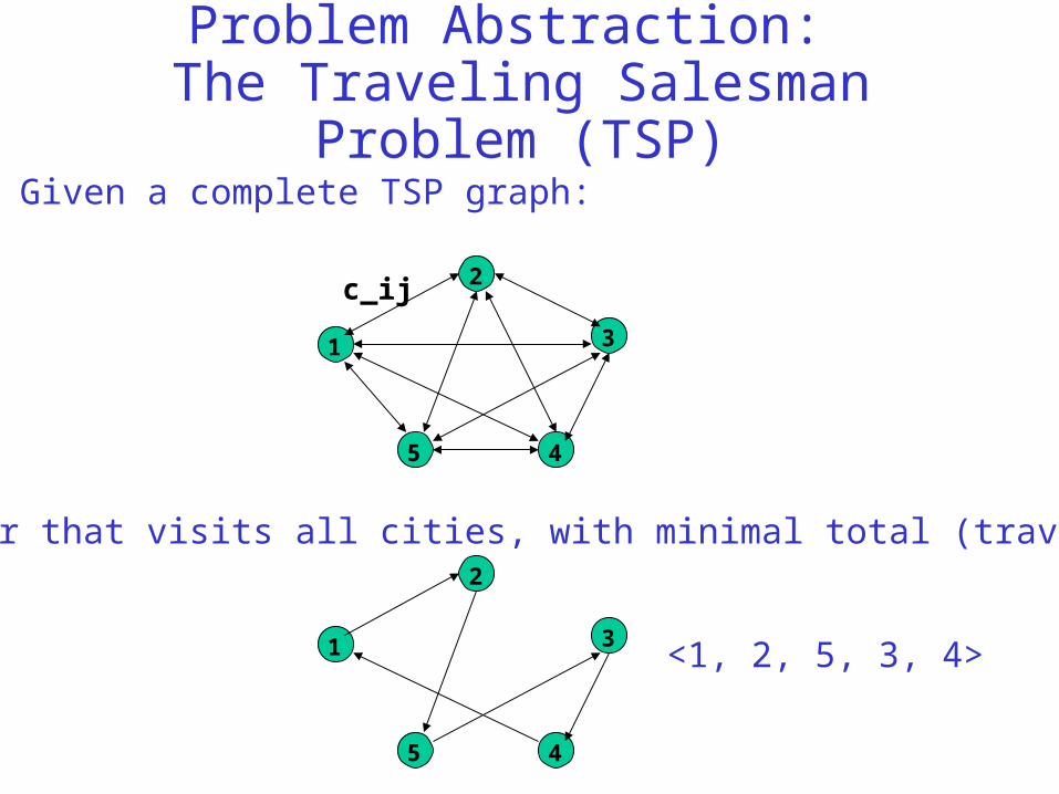
• In the considered application context, the distances c_ij should be computed based on the appropriate distance metric; i.e., rectilinear, Tchebychev, “shortest path”

The closest insertion algorithm:A TSP heuristic (symmetric version)

Initialization:

S_p = <1>; S_a = {2,…,N}; c(j) = 1, j {2,…,N}; n=1;

While n < N do

n = n+1;

Selection step:

j* = argmin_{j S_a} {c_{j,c(j)}};

S_a = S_a \ {j*};

Insertion step:

i* = argmin_{i =1}^|S_p| {c_{[i],j*} + c_{j*,[i mod |S_p|+1]}

- c_{[i],[i mod |S_p|+1]}};

S_p = < [1],…,[i*], j*, [i*+1],…,[n]>;

j S_a, if c_{j,j*} < c_{j,c(j)} then c(j) = j*;

Remarks: 1. [i] denotes the node at i-th position of the constructed sub-tour.

2. If the distances are symmetric and satisfy the triangular inequality, the cost of the solution provided by this heuristic is no worse than twice the optimal cost.

A special case admitting polynomial solution(Ratliff and Rosenthal, Operations Research, 31(3): 507-521, 1983)

Docking stationPicking Aisles

Crossover Aisles

Itemsto bepicked

x

x

xx

x

xx

x

x

x

x

x

A graph-based representation of the underlying topology

x

x

xx

x

xx

x

x

x

x

x

b1 b2 b3 b4 b5 b6

a1 a2 a3 a4 a5 a6

v0

v1

v2

v3

v4

v5

v6

v7

v8

v9

v10

v11

v12

222 2 2

2

7

3

3

2 2 22 2

3

5

3

4 4

6

5

3

6

3

3

15

8

7

0

A picking tour

x

x

xx

x

xx

x

x

x

x

x

b1 b2 b3 b4 b5 b6

a1 a2 a3 a4 a5 a6

v0

v1

v2

v3

v4

v5

v6

v7

v8

v9

v10

v11

v12

222 2 2

2

7

3

3

2 2 22 2

3

5

3

4 4

6

5

3

6

3

3

15

8

7

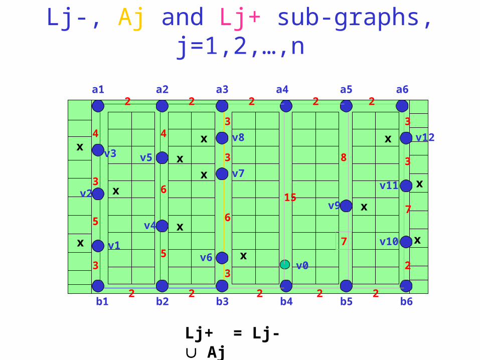
Lj-, Aj and Lj+ sub-graphs, j=1,2,…,n

x

x

xx

x

xx

x

x

x

x

x

b1 b2 b3 b4 b5 b6

a1 a2 a3 a4 a5 a6

v0

v1

v2

v3

v4

v5

v6

v7

v8

v9

v10

v11

v12

222 2 2

2

7

3

3

2 2 22 2

3

5

3

4 4

6

5

3

6

3

3

15

8

7

Lj+ = Lj- Aj

Lj(- or +) PTS (partial tour sub-graph)

x

x

xx

x

xx

x

x

x

x

x

b1 b2 b3 b4 b5 b6

a1 a2 a3 a4 a5 a6

v0

v1

v2

v3

v4

v5

v6

v7

v8

v9

v10

v11

v12

222 2 2

2

7

3

3

2 2 22 2

3

5

3

4 4

6

5

3

6

3

3

15

8

7

L3- PTS : (E, E, 2C)L3+PTS: (U, U, 1C)

A key observationThe only possible characterizations for an Lj (- or +) PTS are the following:• (U, U, 1C)• (0, E, 1C)• (E, 0, 1C)• (E, E, 1C)• (E, E, 2C)• (0, 0, 0C)• (0, 0, 1C)

where the triplet (X, Y, Z) should be interpreted as follows:• X (Y): degree parity for node a_j (b_j) - 0, Even, Uneven (odd)• Z: number of connected components in Lj PTS, excluding the vertices with zero

degree

Going from Lj- to Lj+…

a_j a_j a_ja_j a_j a_j

b_j b_j b_j b_j b_j b_j

(I-i) (I-ii) (I-iii) (I-iv) (I-v) (I-vi)

Going from Lj- to Lj+…(cont.)

Lj- class (I-i) (I-ii) (I-iii) (I-iv) (I-v) (I-vi)a(U,U,1C) (E,E,1C) (U,U,1C) (U,U,1C) (U,U,1C) (U,U,1C) (U,U,1C)(E,0,1C) (U,U,1C) (E,0,1C) (E,E,2C) (E,E,2C) (E,E,1C) (E,0,1C)(0,E,1C) (U,U,1C) (E,E,2C) (0,E,1C) (E,E,2C) (E,E,1C) (0,E,1C)(E,E,1C) (U,U,1C) (E,E,1C) (E,E,1C) (E,E,1C) (E,E,1C) (E,E,1C)(E,E,2C) (U,U,1C) (E,E,2C) (E,E,2C) (E,E,2C) (E,E,1C) (E,E,2C)(0,0,0C)b (U,U,1C) (E,0,1C) (0,E,1C) (E,E,2C) (E,E,1C) (0,0,0C)(0,0,1C)c d (0,0,1C)

a: This is not a feasible configuration if there is any item to be picked in aisle jb: This class can occur only if there are no items to be picked to the left of aisle jc: This class is feasible only if there are no items to be picked to the right of aisle jd: Could never be optimal

TABLE I

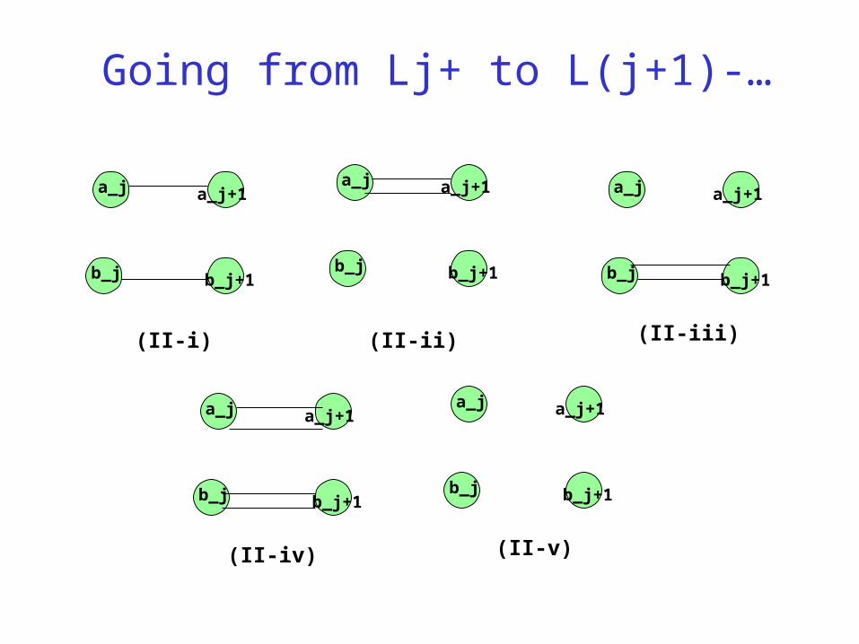
Going from Lj+ to L(j+1)-…

a_j+1a_j

b_j b_j+1

a_j+1a_j

b_j b_j+1

a_j+1a_j

b_j b_j+1

a_j+1a_j

b_j b_j+1

a_j+1a_j

b_j b_j+1

(II-i) (II-ii) (II-iii)

(II-iv) (II-v)

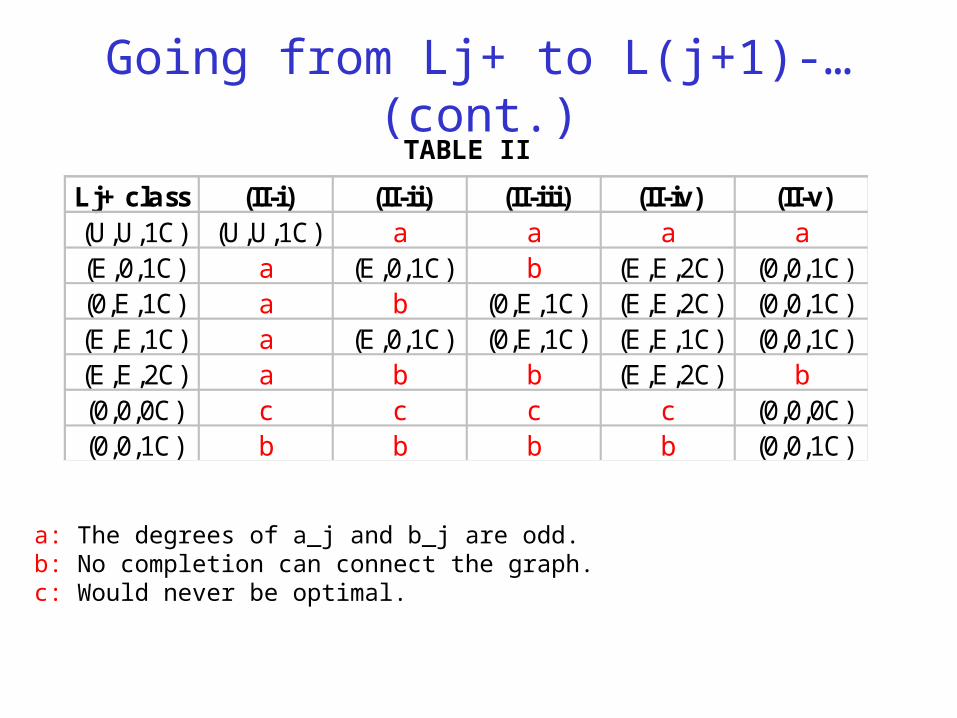
Going from Lj+ to L(j+1)-…(cont.)

Lj+ class (II-i) (II-ii) (II-iii) (II-iv) (II-v)(U,U,1C) (U,U,1C) a a a a(E,0,1C) a (E,0,1C) b (E,E,2C) (0,0,1C)(0,E,1C) a b (0,E,1C) (E,E,2C) (0,0,1C)(E,E,1C) a (E,0,1C) (0,E,1C) (E,E,1C) (0,0,1C)(E,E,2C) a b b (E,E,2C) b(0,0,0C) c c c c (0,0,0C)(0,0,1C) b b b b (0,0,1C)

a: The degrees of a_j and b_j are odd.b: No completion can connect the graph.c: Would never be optimal.

TABLE II

A polynomial-complexity algorithm for computing a minimum-length tour

• Initialization: L1- PTS = null graph for every class type

• For <L1+, L2-, L2+,…,Ln-, Ln+)

– compute a minimum-length PTS for each of the seven classes, using the minimum-length PTS’s constructed in the previous stage, and the information provided in Tables I and II.

– Remark: For case (I-iv), a minimum-length PTS is obtained by putting the gap between the two adjacent v_i’s in aisle j that are farthest apart.

• A minimum-length tour is defined by a minimum-length Ln+ PTS.

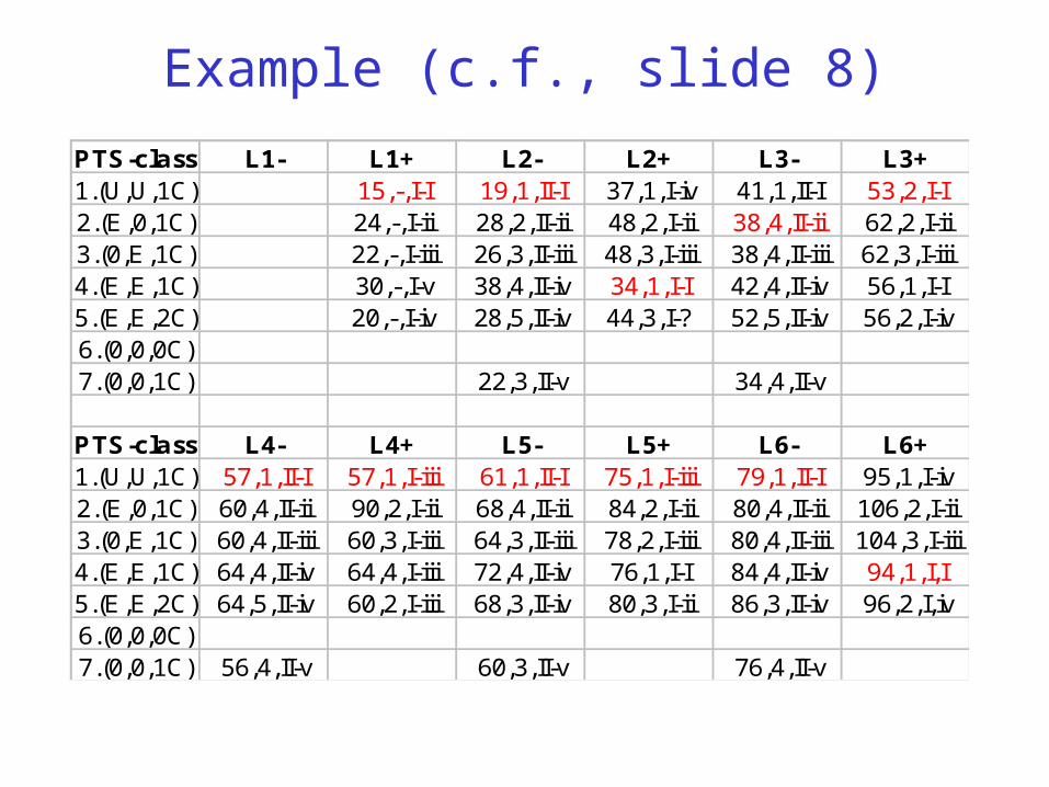
Example (c.f., slide 8)

PTS-class L1- L1+ L2- L2+ L3- L3+1.(U,U,1C) 15,-,I-I 19,1,II-I 37,1,I-iv 41,1,II-I 53,2,I-I2.(E,0,1C) 24,-,I-ii 28,2,II-ii 48,2,I-ii 38,4,II-ii 62,2,I-ii3.(0,E,1C) 22,-,I-iii 26,3,II-iii 48,3,I-iii 38,4,II-iii 62,3,I-iii4.(E,E,1C) 30,-,I-v 38,4,II-iv 34,1,I-I 42,4,II-iv 56,1,I-I5.(E,E,2C) 20,-,I-iv 28,5,II-iv 44,3,I-? 52,5,II-iv 56,2,I-iv6.(0,0,0C)7.(0,0,1C) 22,3,II-v 34,4,II-v

PTS-class L4- L4+ L5- L5+ L6- L6+1.(U,U,1C) 57,1,II-I 57,1,I-iii 61,1,II-I 75,1,I-iii 79,1,II-I 95,1,I-iv2.(E,0,1C) 60,4,II-ii 90,2,I-ii 68,4,II-ii 84,2,I-ii 80,4,II-ii 106,2,I-ii3.(0,E,1C) 60,4,II-iii 60,3,I-iii 64,3,II-iii 78,2,I-iii 80,4,II-iii 104,3,I-iii4.(E,E,1C) 64,4,II-iv 64,4,I-iii 72,4,II-iv 76,1,I-I 84,4,II-iv 94,1,I,I5.(E,E,2C) 64,5,II-iv 60,2,I-iii 68,3,II-iv 80,3,I-ii 86,3,II-iv 96,2,I,iv6.(0,0,0C)7.(0,0,1C) 56,4,II-v 60,3,II-v 76,4,II-v

Example: The optimal tour

x

x

xx

x

xx

x

x

x

x

x

b1 b2 b3 b4 b5 b6

a1 a2 a3 a4 a5 a6

v0

v1

v2

v3

v4

v5

v6

v7

v8

v9

v10

v11

v12

222 2 2

2

7

3

3

2 2 22 2

3

5

3

4 4

6

5

3

6

3

3

15

8

7

0

k-STRIP: A computationally simple heuristic for rectangular areas

x

x

x

x

x

x

x

x

x

x

I/O point

x

x

• When A is the unit square, an optimized k = (n/2) , and for this value, the worst-case tour length generated by the heuristic is between 1.075n and 1.414 n, for large n.• The computational complexity is O(n logn).• Supowit, Reingold and Plaisted, “The traveling salesman problem and minimum matching in the unit square”, SIAM J. Computing, 12(1): 144-156, 1983.

The bin-numbering heuristic(Bartholdi and Platzman, Material Flow, 4: 247-254, 1988)

• Basic idea: Number bins / storage locations in a way that filling the orders by visiting the associated bins in increasing numbers will lead to efficient routings.

• Advantages:– Once the numbering is established, developing the order routes

becomes extremely simple.

– Easy to adjust routes dynamically upon the arrival of new orders.

• Basic underlying problem:How do you establish good bin-numbering schemes?

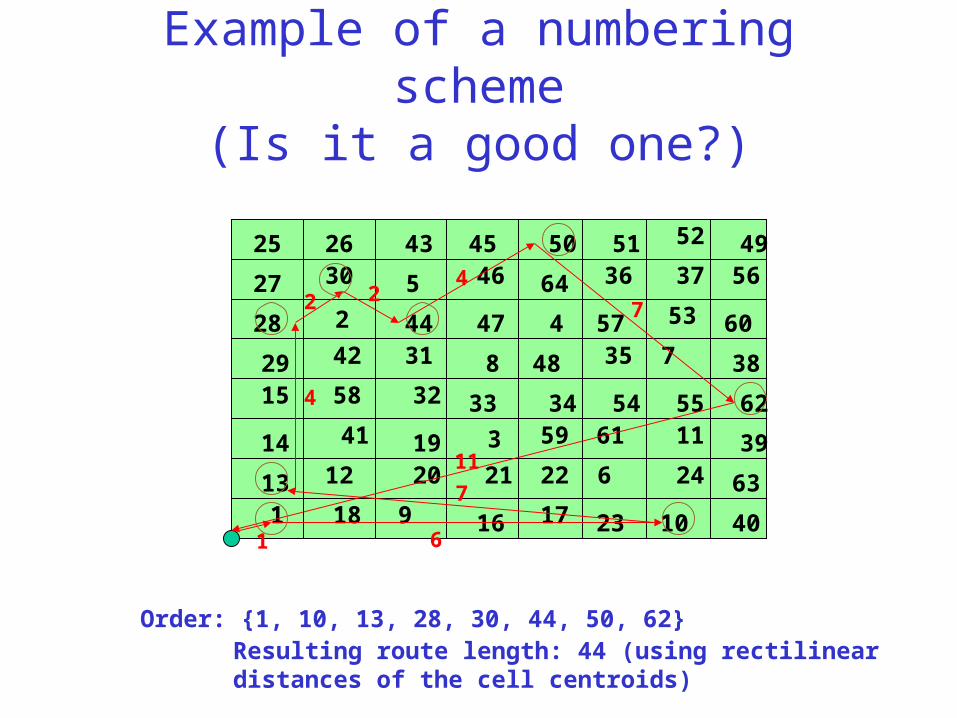
Example of a numbering scheme(Is it a good one?)

Order: {1, 10, 13, 28, 30, 44, 50, 62}

1

2

3

4

5

6

78

9 10

11

1213

14

15

16 1718

1920 21 22

23

24

25 26

27

28

29

30

31

32 33 34

35

36 37

38

39

40

41

42

43

64

44

4546

47

48

4950 51 52

53

54 55

56

57

58

59

60

6162

63

1 6

7

4

2 24

7

11

Resulting route length: 44 (using rectilinear distances of the cell centroids)

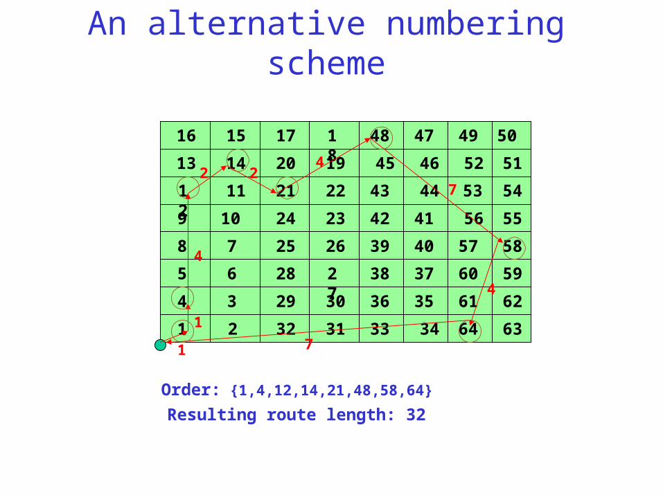
An alternative numbering scheme

1 2

34

5 6

78

9 10

1112

13

1516 17 18

1920

21 22

2324

25 26

2728

29 30

3132 33 34

3536

3738

39 40

4142

43

64

44

45 46

4748 49 50

5152

53 54

5556

57 58

5960

61 62

63

14

Order: {1,4,12,14,21,48,58,64}

1

1

4

2 24

7

4

7

Resulting route length: 32

Key concept: Space-filling curves(see also http://www.isye.gatech.edu/faculty/John_Bartholdi/mow/mow.html)

• Closed curves that sweep the entire region while preserving nearness.• Technically, they define a continuous mapping of the unit interval on the unit square.• Typical example: Sierpinski’s space-filling curve:

The Sierpinski space-filling curve

Applying the Sierpinski space-filling curve in the previous bin-numbering example

1

2 3

45

6 7

8

9 10

1112

13

1516

17

1819

20 21

22

23 24

25

2627

28 29

3031

32 33

34

35 36

37

38 39

404142

43

64

44 45 46

4748

49 50

5152

53

545556

57 58

596061

62

63

14

Order: {1,2,13,17,18,32,46,52}

Resulting route length: 34

1

1

6

2

2

4

7

4

7

Some properties of the bin-numbering schemes based on the Sierpinski

space-filling curve

• If n locations are to be visited throughout a warehouse of area A, then the length of the retrieval route is at most (2nA).

• If every location is equally likely to be visited, then on average, the retrieval route produced by the corresponding bin-numbering heuristic will be 25% longer than the shortest possible route length.

• The above results have been derived using the Euclidean metric for measuring the traveling distances, but they are robust with respect to other metrics that preserve “closeness” according to the Euclidean metric.

Characterizing the best bin-numbering scheme...

• …is computationally very hard.• Some good schemes can be obtained through interchange techniques (e.g., 2 or

3-opt), where the efficiency of each of the considered schemes is evaluated through simulation.

• The optimal bin-numbering scheme depends on:– the underlying geometry of the picking facility

– the frequency with which the various storage locations are visited (and therefore, the applying storage policy)

• In general, the logic underlying the utilization of the space-filling curves is more useful / pertinent for storage areas with small visitation frequencies for their locations.

• For areas with high visitation frequencies, numbering schemes suggesting an exhaustive sweeping of the region tend to perform better (c.f., Bartholdi & Platzman, pg. 252).

Bin-numbering in structures with complicated geometry

When the considered area has a structure too complex to measure traveling effort by Euclidean or a relative metric, the logic underlying the application of space-filling curves to bin-numbering can be applied in a hierarchical fashion:

• separate the entire area under consideration to smaller areas of simpler geometry;

• design a numbering sequence for each of these areas using the space-filling curve logic;

• develop a visiting sequence for the areas developed in step 1, by passing a space-filling curve among their I/O points.

Order Batching

(based on De Koster et. al., “Efficient orderbatching methods in warehouses”, Inlt. Jrnl of Prod. Res., Vol. 37, No. 7, pgs 1479-

1504, 1999)

Problem Description

• Given a set of orders, cluster them into batches - i.e., subsets of orders that are to be picked simultaneously by one picker at a single trip - s.t. – the total traveling distance / time is minimized– while each batch does not exceed some measure of the picker

capacity (e.g., number of items / volume of the resulting batch, number of distinct orders in a batch)

• Theoretically, the problem can be solved by: – enumerating all feasible partitions of the given order set into batches;

– evaluating the total traveling distance / time for each partition;

– picking the partition with the smallest traveling distance / time.

• However, combinatorial explosion of partitions => heuristics

Order-Batching Heuristics

Naive Intelligent

FCFS Seed Algorithms Savings Algorithms

(Batches are builtsequentially, one ata time)

(All batches are builtsimultaneously, by merging partially developed batches)

(Orders are clusteredbased on the sequenceof their appearance)

The generic structure for seed algorithms

• While there are unprocessed orders,– Pick a new seed order according to some seed selection

rule;– while there are unprocessed orders and the batch has not

reached the imposed capacity limit• pick a new order to be added to the batch according to

an order addition rule;• add the selected order to the batch, provided that the

imposed capacity limit is not violated;• (update the batch seed to the union of the previous batch

seed and the new order)

Typical seed selection rules

• Random selection• the order with the farthest item (w.r.t. the shipping station)• the order with the largest number of aisles to be visited• the order with the largest aisle range (absolute difference between the

most left aisle number and the most right aisle number to be visited)• the order with the largest number of items• the order with the longest travel time

• Remark: If the batch seed is updated after every order addition, the algorithm is characterized as dynamic or cumulative mode; ow., it is said to be static or single mode.

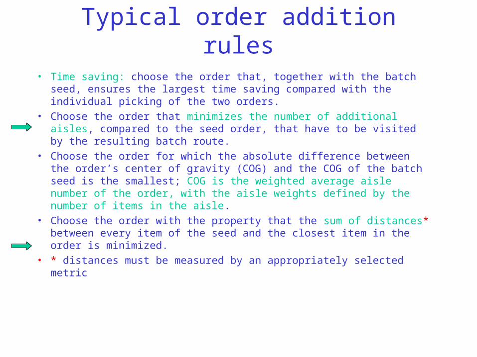
Typical order addition rules

• Time saving: choose the order that, together with the batch seed, ensures the largest time saving compared with the individual picking of the two orders.

• Choose the order that minimizes the number of additional aisles, compared to the seed order, that have to be visited by the resulting batch route.

• Choose the order for which the absolute difference between the order’s center of gravity (COG) and the COG of the batch seed is the smallest; COG is the weighted average aisle number of the order, with the aisle weights defined by the number of items in the aisle.

• Choose the order with the property that the sum of distances* between every item of the seed and the closest item in the order is minimized.

• * distances must be measured by an appropriately selected metric

The (standard) savings algorithm

• Initialization: B: = order set (each order defines its own batch)• Repeat

– For each pair (i,j) in the current batch set B• compute the time savings s_ij = t_i + t_j - t_ij, where t_i/j is the time

required for picking batch i/j and t_ij is the time required for picking the batch resulting from the merging of batches i and j.

– Rank batch pairs (i,j) in decreasing s_ij.– Pick the first batch pair (i,j) in the ranked list, for which the merging of its

constituent batches does not violate the imposed capacity limit, and merge batches i and j: B := (B-{i,j}) U {i+j}

until no further batch merging is possible.

• Remark: The algorithm result depends on the adopted pick sequencing rule.

Some findings regarding the (relative) performance of the presented batch

algorithms (De Koster et. al.)• Intelligent batching leads to significant improvements compared to single-order picking

and naïve batching schemes.

• In seed algorithms, dynamic seed definition leads to better performance than static seed definition.

• The best seed selection rules are focusing on orders dispersed over a large number of aisles and involving long travel times.

• The best order addition rules (c.f. corresponding slide) tend also to be the most robust (i.e., they yield the best results in all warehouse configurations considered in the simulation).

• Savings algorithms have good performance, in general, but they tend to be computationally more expensive than seed algorithms.

• The performance of the applied batching algorithm has a significant dependence on the adopted pick sequencing rule.

• The largest the number of orders per batch (the batch capacity limit), the smaller the savings from intelligent batching (and therefore, simpler batching schemes become more eligible candidates)

Warehouse Zoning

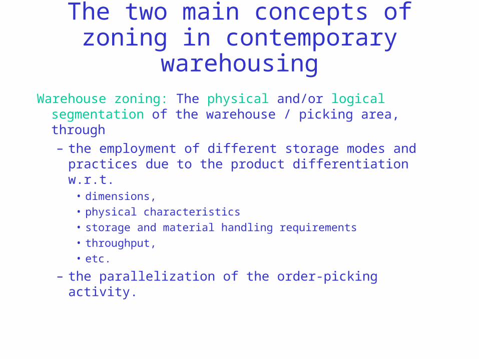
The two main concepts of zoning in contemporary warehousing

Warehouse zoning: The physical and/or logical segmentation of the warehouse / picking area, through

– the employment of different storage modes and practices due to the product differentiation w.r.t.

• dimensions,

• physical characteristics

• storage and material handling requirements

• throughput,

• etc.

– the parallelization of the order-picking activity.

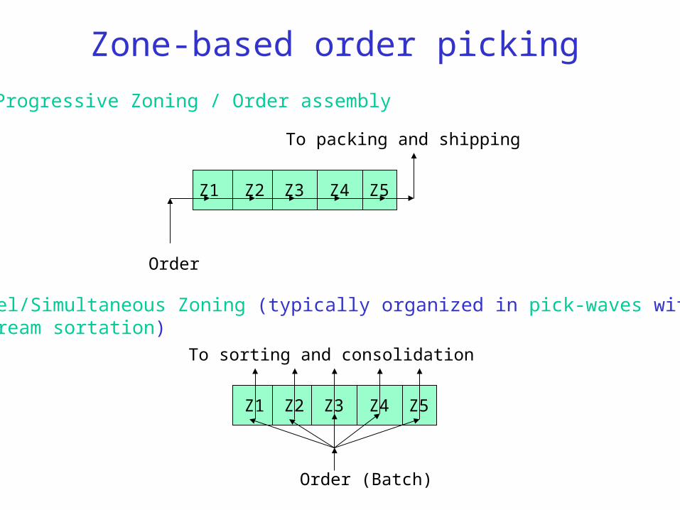
Zone-based order picking

Progressive Zoning / Order assembly

Parallel/Simultaneous Zoning (typically organized in pick-waves with downstream sortation)

Order

To packing and shipping

Z1 Z2 Z3 Z4 Z5

Order (Batch)

To sorting and consolidation

Z1 Z2 Z3 Z4 Z5

Defining effective zones for order-picking• Main objective: Try to achieve maximum utilization of the picking

resources, by distributing “equally” the total (picking) workload among the defined zones.

• However, the warehouse picking environment usually is a very dynamic environment; workload profiles are constantly changing.

• Existing zoning systems seek to balance the average workloads across zones, based on some hypothetical order work-content and worker behavioral models.

• Furthermore, constant zone redefinition requires a lot of effort from, both, the warehouse management (who must keep track of all the workload changes and re-establish the zones) and the warehouse pickers (who must adjust to the new policies).

• Very limited scientific literature.

Bucket Brigades( c.f. Bartholdi & Hackman, Chpt. 10)

• A dynamic self-balancing scheme for progressive zoning.

• The three main requirements of bucket brigades:

– Carry work forward, from station to station, until someone takes over your work.

– If a worker catches up to his successor, he remains idle until the station is available (i.e., no overpassing is allowed)

– Workers are sequenced from slowest to fastest.

The self-balancing property of bucket brigades

Theorem: The line operation under the three main requirements of bucket brigades, converges to a balanced partition of the effortwherein • the fraction of work performed by the i-th worker is equal to

v_i / _{j=1}^n v_j• and the line production rate is equal to

_{j=1}^n v_j items per unit time.