Journal of Physics Conference Series

OPEN ACCESS

Orbital Disturbance Analysis due to the LunarGravitational Potential and Deviation Minimizationthrough the Trajectory Control in Closed LoopTo cite this article L D Gonccedilalves et al 2013 J Phys Conf Ser 465 012013

View the article online for updates and enhancements

You may also likeSpecial issue on applied neurodynamicsfrom neural dynamics to neuralengineeringHillel J Chiel and Peter J Thomas

-

LARRMACC Conference Liverpool 5November 1998S M Clark

-

Summary of PapersSerge Gauthier Snezhana I Abarzhi andKatepalli R Sreenivasan

-

Recent citationsLifetime of a spacecraft around asynchronous system of asteroids using adipole modelLeonardo Barbosa Torres dos Santos et al

-

Orbital Trajectories in Deimos VicinityConsidering Perturbations of GravitationalOriginL D Gonccedilalves et al

-

Mapping the Galilean moonrsquos disturbanceacting on a spacecraftrsquos trajectoryNatasha Camargo de Araujo and EvandroMarconi Rocco

-

This content was downloaded from IP address 18554100166 on 14012022 at 1559

Orbital Disturbance Analysis due to the Lunar Gravitational

Potential and Deviation Minimization through the Trajectory

Control in Closed Loop

L D Gonccedilalves1 E M Rocco

1 and R V de Moraes

2

1 Instituto Nacional de Pesquisas Espaciais INPE Satildeo Joseacute dos Campos Brazil

2 Universidade Federal de Satildeo Paulo UNIFESP Satildeo Joseacute dos Campos Brazil

E-mail lianadgongmailcom evandro_mryahoocombr

rodolphovilhenagmailcom

Abstract A study evaluating the influence due to the lunar gravitational potential modeled

by spherical harmonics on the gravity acceleration is accomplished according to the model

presented in Konopliv (2001) This model provides the components x y and z for the gravity

acceleration at each moment of time along the artificial satellite orbit and it enables to consider

the spherical harmonic degree and order up to100 Through a comparison between the gravity

acceleration from a central field and the gravity acceleration provided by Konoplivrsquos model it

is obtained the disturbing velocity increment applied to the vehicle Then through the inverse

problem the Keplerian elements of perturbed orbit of the satellite are calculated allowing the

orbital motion analysis Transfer maneuvers and orbital correction of lunar satellites are

simulated considering the disturbance due to non-uniform gravitational potential of the Moon

utilizing continuous thrust and trajectory control in closed loop The simulations are performed

using the Spacecraft Trajectory Simulator-STRS Rocco (2008) which evaluate the behavior of

the orbital elements fuel consumption and thrust applied to the satellite over the time

1 Introduction

If the existence of disturbing forces were ignored the orbital motion would be a conic set in a fixed

plane with constant size and eccentricity However the existence of such forces tends to cause

variations in the elements that characterize the orbit of an artificial satellite In some cases this

variations should be corrected to enable the mission accomplishment

In order to study the perturbations due to non-sphericity of the lunar gravitational field it is used the

LP100K model so that an analysis of the influence of the degree and order of the harmonics in the

artificial lunar satellite orbit is done These disturbance effects are inserted into the Spacecraft

Trajectory Simulator (STRS) in order to control the trajectory and minimize the deviations The

correction of the errors in the orbit is made by the STRS using a continuous propulsion system

controlled in closed loop

XVI Brazilian Colloquium on Orbital Dynamics IOP PublishingJournal of Physics Conference Series 465 (2013) 012013 doi1010881742-65964651012013

Content from this work may be used under the terms of the Creative Commons Attribution 30 licence Any further distributionof this work must maintain attribution to the author(s) and the title of the work journal citation and DOI

Published under licence by IOP Publishing Ltd 1

2 Lunar Gravitational Potential

The moons gravitational potential is expressed by the coefficients of normalized spherical harmonics

given by Equation (1) (Konopliv 2001 Kuga 2011)

(1)

where is the degree is the order is the gravitational constant and r is the lunar equatorial radius

are the fully normalized associated Legendre polynomials is the reference radius Moon is

the latitude and is the longitude

3 The Model LP100K

The lunar gravitational field was determined using data from some previous lunar missions One of the

most important missions was the Lunar Prospector (1998-1999) The LP was the third mission in

NASAs exploration program called Discovery and provided the first measurement of the moon

gravitational field The information about the gravity field comes from the long-term effect observed

in the satellite orbit (Konopliv 2001)

The model presented in Konoplivrsquos called GRAVITYSPHERICALHARMONIC is a representation of

the spherical harmonics due to planetary gravity based on the gravitational potential of the planet

given by the Equation (1)

The output calculated by the model includes the values of gravity in meters per squared second on the

axes x y and z From the values of the gravity acceleration it is possible to obtain the state variables

and hence the orbital elements that characterize the satellite orbit

Using the GRAVITYSPHERICALHARMONIC model it was created the Gravity_Moon subroutine

used for the simulations of the artificial satellites orbital motion around the Moonrsquos surface

4 Study of oblateness and equatorial ellipticity effects on the lunar orbit of an artificial satellite

The Figure 1 shows the value obtained for the resulting of gravity acceleration on a satellite for each

value of degree and order from 1 up to 100 at an altitude around 250 km

We observe by the Figure 1 that the value of the gravity acceleration on the artificial satellite tends to

stabilize at a value close to 12250 mssup2 when considering values of degree and order bigger than 15

However we can also reach this approximate value using the degree and order 2

It is important to adopt the highest possible value for degree and order since by the use of many terms

of the spherical harmonics we can represent the imperfections of the bodies format in a more accurate

way However for a first analysis the value 2 for degree and order could be adopted

Figura 1 Gravity acceleration due spherical harmonics

0 20 40 60 80 100 120 140 160 18012255

12256

12257

12258

12259

1226

12261LP100K Aceleraccedilatildeo da Gravidade 2

Grau e Ordem

Acele

raccedilatildeo d

a G

ravid

ade (

ms

2)

XVI Brazilian Colloquium on Orbital Dynamics IOP PublishingJournal of Physics Conference Series 465 (2013) 012013 doi1010881742-65964651012013

2

5 Results

In this section we present the results of two different simulations both performed during 86400 s

considering the terms due to non-homogeneity of the lunar gravitational field and the value 2 to

degree and order In both cases the continuous propulsion system are trigged when the simulation

time reaches 2000 s and is turned off when the semi-major axis reaches the value of 4000 km

In the first simulation the satellite leaves a low lunar orbit to reaches a high orbit using continuous

tangential thrust with magnitude of 2N as seen in Figure 2 In the second simulation it is considered

the application of higher thrust (20 N) applied over an arc of 5 degrees around the periapse as seen in

Figure 3 In the simulations 1 and 2 were considered the effects of disturbance and the action of the

thrusters simultaneously whose initial conditions considered were semi-major axis 1800000 m

eccentricity 0001 inclination 45ordm right ascension of the ascending node 20ordm argument the periapse

100ordm mean anomaly 1ordm

Figure 2 Trajectory of the satellite in

simulation 1 Figure 3 Trajectory of the satellite in

simulation 2

The Figure 4 presents the case where only the correction of the trajectory is considered to illustrate the

ability of the control system to deal with the effect of orbital perturbation In this case the aim of the

control system is minimize the effects of the perturbations acting on the satellite In this simulation

only the effects of lunar oblateness and equatorial ellipticity were considered until degree 2 From

Figure 4 we can notice that the force applied by the propulsion system acts toward to correct the

effects caused by the disturbing force The figure shows the results for x axis but a similar behavior is

obtained for y and z axes Therefore it was verified that the control system is able to deal with the

disturbance effects on the lunar satellite when considering the effects caused by the non-homogeneity

of the lunar gravitational field

Figure 4 - Control signal and disturbance signal on the satellite (x axis)

0 1 2 3 4 5 6 7 8 9

x 104

-15

-1

-05

0

05

1

15x 10

-3

Tempo (s)

Contr

ole

(m

s)

sinal de controle

sinal da perturbaccedilatildeo

controle + perturbaccedilatildeo

XVI Brazilian Colloquium on Orbital Dynamics IOP PublishingJournal of Physics Conference Series 465 (2013) 012013 doi1010881742-65964651012013

3

The following results obtained in the simulations 1 and 2 will be exposed to the study of the behavior

of the orbital elements propellant mass thrust applied on the satellite altitude reached and the

disturbance acting on the satellite along the trajectory

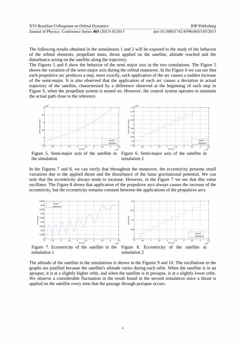
The Figures 5 and 6 show the behavior of the semi major axis in the two simulations The Figure 5

shows the variation of the semi-major axis during the orbital maneuver In the Figure 6 we can see that

each propulsive arc produces a step more exactly each application of the arc causes a sudden increase

of the semi-major It is also observed that the application of each arc causes a deviation in actual

trajectory of the satellite characterized by a difference observed at the beginning of each step in

Figure 6 when the propellant system is turned on However the control system operates to maintain

the actual path close to the reference

Figure 5 Semi-major axis of the satellite in

the simulation Figure 6 Semi-major axis of the satellite in

simulation 2

In the Figures 7 and 8 we can verify that throughout the maneuver the eccentricity presents small

variations due to the applied thrust and the disturbance of the lunar gravitational potential We can

note that the eccentricity always tends to increase However in the Figure 7 we see that this value

oscillates The Figure 8 shows that application of the propulsive arcs always causes the increase of the

eccentricity but the eccentricity remains constant between the applications of the propulsive arcs

Figure 7 Eccentricity of the satellite in the

simulation 1 Figure 8 Eccentricity of the satellite in

simulation 2

The altitude of the satellite in the simulations is shown in the Figures 9 and 10 The oscillations in the

graphs are justified because the satellites altitude varies during each orbit When the satellite is in an

apoapse it is at a slightly higher orbit and when the satellite is in periapse is at a slightly lower orbit

We observe a considerable fluctuation in the result found in the second simulation since a thrust is

applied on the satellite every time that the passage through periapse occurs

0 05 1 15 2 25 3 35 4 45

x 105

15

2

25

3

35

4x 10

6

Time (s)

Sem

i-m

ajo

r axis

(m)

current

reference

0 05 1 15 2 25 3 35 4 45

x 105

175

18

185

19

195

2

205

21

215

22x 10

6

Time (s)

Sem

i-m

ajo

r axis

(m)

current

reference

0 05 1 15 2 25 3 35 4 45

x 105

0

0005

001

0015

002

0025

003

0035

004

0045

Time (s)

Eccentr

icity

current

reference

0 05 1 15 2 25 3 35 4 45

x 105

0

005

01

015

02

Time (s)

Eccentr

icity

current

reference

XVI Brazilian Colloquium on Orbital Dynamics IOP PublishingJournal of Physics Conference Series 465 (2013) 012013 doi1010881742-65964651012013

4

Figure 9 Altitude of the satellite during

simulation 1 Figure 10 Altitude of the satellite during

simulation 2

The Figures 11 and 12 show the disturbing force applied in the lunar satellite during the simulations

We can note that the intensity of the disturbing force decreases with the time since the semi-major

axis is increasing along the time in other words the distant from the lunar surface is increasing and

therefore the disturbing due to the non-uniform distribution of mass of the Moon is becoming less

relevant

Figure 11 Disturbance in the orbit of a lunar

satellite due to non-sphericity of the

gravitational field during simulation 1

Figure 12 Disturbance in the orbit of a lunar

satellite due to non-sphericity of the

gravitational field during simulation 2

In the Figures 13 and 14 we can observe thrust applied during the simulations It is possible to verify

the thrust force applied in the three axes and the control system acts separately on each axis Note in

the Figure 13 that the operation is finished when according to the Figure 5 the semi-major axis

reaches the value of 4000 km At this point the propellant is turned off and the thrust applied tends to

zero From the Figure 14 is also possible to realize that with the passage of time the distance between

two peaks or two valleys of the generated wave increases this occurs because the semi-major axis

increases during the simulation so the period of the orbit also increases

Figure 13 Thrust applied to the satellite

during simulation 1 Figure 14 Thrust applied to the satellite

during simulation 2

0 05 1 15 2 25 3 35 4 45

x 105

0

500

1000

1500

2000

2500

Time (s)

Altitude (

km

)

0 05 1 15 2 25 3 35 4 45

x 105

0

100

200

300

400

500

600

700

800

900

Time (s)

Altitude (

km

)

0 05 1 15 2 25 3 35 4 45

x 105

-3

-2

-1

0

1

2

3

4x 10

-3

Time (s)

Dis

turb

ing (

ms

)

x axis

y axis

z axis

disturbing

0 05 1 15 2 25 3 35 4 45

x 105

-3

-2

-1

0

1

2

3

4x 10

-3

Time (s)

Dis

turb

ing (

ms

)

x axis

y axis

z axis

disturbing

0 05 1 15 2 25 3 35 4 45

x 105

-3

-2

-1

0

1

2

3

4

Time (s)

Applie

d t

hru

st

(N)

x axis

y axis

z axis

thrust

0 05 1 15 2 25 3 35 4 45

x 105

-30

-20

-10

0

10

20

30

40

Time (s)

Applie

d t

hru

st

(N)

x axis

y axis

z axis

thrust

XVI Brazilian Colloquium on Orbital Dynamics IOP PublishingJournal of Physics Conference Series 465 (2013) 012013 doi1010881742-65964651012013

5

From the Figures 15 and 16 we can analyze the fuel consumption in the simulations We can note in

the Figure 15 that at time 2000 s the propulsion system is turned on and at the instant of 83000 s is

turned off (semi-major axis reaches 4000 km) thus the fuel consumption tends to stabilize In the

Figure 16 we can realize that each application of propulsive arc imply a significant fuel consumption

which tends to stabilize until the application of the next arc however the consumption do not ceases to

grow between arcs because the control system must act to deal with the perturbative effects that do not

cease between arcs

Figure 15 Mass of propellant expended during

simulation 1 Figure 16 Mass of propellant expended during

simulation 2

6 Conclusions

The results showed that the Spacecraft Trajectory Simulator developed to analyze space missions

using a closed loop control system and correct the trajectory by the application of continuous thrust is

able to minimize the deviations in the path of the spacecraft when considering perturbations in the

orbit due to the lunar gravitational potential of the Moon

We can observe that the deviations in state variables values were always small in other words the

control system was able to reduce the error in the state variables through the action of thrusters

The Figures 11 and 12 showed that the disturbance on an artificial satellite due to the non-uniform

distribution of mass of the Moon is not stable requiring intense performance of the control system to

mitigate deviations in the trajectory

This study results are consistent with the results presented in Konopliv (2001) showing the correlation

between the lunar gravitational acceleration and topography and the variation of the gravity

acceleration due to non-uniform moon mass distribution The vehicle orbital elements oscillation

magnitude are in accordance with the gravity acceleration variation for the model presented Konopliv

References

[1] KAULA W M Theory of satellite geodesy applications of satellites to geodesy Waltham

MA Blaisdell 1966 124 p

[2] KONOPLIV A S ASMAR S W CARRANZA E SJOGREN W L YUAN D N

Recent gravity models as a result of the lunar prospector mission Icarus Vol 150 pp 1-18

Academic Press 2001

[3] KUGA HK CARRARA V KONDAPALLI R R Sateacutelites Artificiais ndash Movimento

Orbital INPE - Satildeo Joseacute dos Campos 2011 111 p Prado A F B A Broucke R A 1993

Juacutepiter Swing-By trajectories passing near the Earth

[4] ROCCO E M Perturbed orbital motion with a PID control system for the

trajectory In Coloacutequio Brasileiro de Dinacircmica Orbital 14 Aacuteguas de Lindoacuteia2008

[5] TAFF L G Celestial mechanics a computational guide for the practitioner New York

NY John Wiley 1985 520 p

0 05 1 15 2 25 3 35 4 45

x 105

0

1

2

3

4

5

6

7

Time (s)

Tota

l pro

pella

nt

mass (

Kg)

0 05 1 15 2 25 3 35 4 45

x 105

0

05

1

15

2

25

Time (s)

Tota

l pro

pella

nt

mass (

Kg)

XVI Brazilian Colloquium on Orbital Dynamics IOP PublishingJournal of Physics Conference Series 465 (2013) 012013 doi1010881742-65964651012013

6

2 Lunar Gravitational Potential

The moons gravitational potential is expressed by the coefficients of normalized spherical harmonics

given by Equation (1) (Konopliv 2001 Kuga 2011)

(1)

where is the degree is the order is the gravitational constant and r is the lunar equatorial radius

are the fully normalized associated Legendre polynomials is the reference radius Moon is

the latitude and is the longitude

3 The Model LP100K

The lunar gravitational field was determined using data from some previous lunar missions One of the

most important missions was the Lunar Prospector (1998-1999) The LP was the third mission in

NASAs exploration program called Discovery and provided the first measurement of the moon

gravitational field The information about the gravity field comes from the long-term effect observed

in the satellite orbit (Konopliv 2001)

The model presented in Konoplivrsquos called GRAVITYSPHERICALHARMONIC is a representation of

the spherical harmonics due to planetary gravity based on the gravitational potential of the planet

given by the Equation (1)

The output calculated by the model includes the values of gravity in meters per squared second on the

axes x y and z From the values of the gravity acceleration it is possible to obtain the state variables

and hence the orbital elements that characterize the satellite orbit

Using the GRAVITYSPHERICALHARMONIC model it was created the Gravity_Moon subroutine

used for the simulations of the artificial satellites orbital motion around the Moonrsquos surface

4 Study of oblateness and equatorial ellipticity effects on the lunar orbit of an artificial satellite

The Figure 1 shows the value obtained for the resulting of gravity acceleration on a satellite for each

value of degree and order from 1 up to 100 at an altitude around 250 km

We observe by the Figure 1 that the value of the gravity acceleration on the artificial satellite tends to

stabilize at a value close to 12250 mssup2 when considering values of degree and order bigger than 15

However we can also reach this approximate value using the degree and order 2

It is important to adopt the highest possible value for degree and order since by the use of many terms

of the spherical harmonics we can represent the imperfections of the bodies format in a more accurate

way However for a first analysis the value 2 for degree and order could be adopted

Figura 1 Gravity acceleration due spherical harmonics

0 20 40 60 80 100 120 140 160 18012255

12256

12257

12258

12259

1226

12261LP100K Aceleraccedilatildeo da Gravidade 2

Grau e Ordem

Acele

raccedilatildeo d

a G

ravid

ade (

ms

2)

XVI Brazilian Colloquium on Orbital Dynamics IOP PublishingJournal of Physics Conference Series 465 (2013) 012013 doi1010881742-65964651012013

2

5 Results

In this section we present the results of two different simulations both performed during 86400 s

considering the terms due to non-homogeneity of the lunar gravitational field and the value 2 to

degree and order In both cases the continuous propulsion system are trigged when the simulation

time reaches 2000 s and is turned off when the semi-major axis reaches the value of 4000 km

In the first simulation the satellite leaves a low lunar orbit to reaches a high orbit using continuous

tangential thrust with magnitude of 2N as seen in Figure 2 In the second simulation it is considered

the application of higher thrust (20 N) applied over an arc of 5 degrees around the periapse as seen in

Figure 3 In the simulations 1 and 2 were considered the effects of disturbance and the action of the

thrusters simultaneously whose initial conditions considered were semi-major axis 1800000 m

eccentricity 0001 inclination 45ordm right ascension of the ascending node 20ordm argument the periapse

100ordm mean anomaly 1ordm

Figure 2 Trajectory of the satellite in

simulation 1 Figure 3 Trajectory of the satellite in

simulation 2

The Figure 4 presents the case where only the correction of the trajectory is considered to illustrate the

ability of the control system to deal with the effect of orbital perturbation In this case the aim of the

control system is minimize the effects of the perturbations acting on the satellite In this simulation

only the effects of lunar oblateness and equatorial ellipticity were considered until degree 2 From

Figure 4 we can notice that the force applied by the propulsion system acts toward to correct the

effects caused by the disturbing force The figure shows the results for x axis but a similar behavior is

obtained for y and z axes Therefore it was verified that the control system is able to deal with the

disturbance effects on the lunar satellite when considering the effects caused by the non-homogeneity

of the lunar gravitational field

Figure 4 - Control signal and disturbance signal on the satellite (x axis)

0 1 2 3 4 5 6 7 8 9

x 104

-15

-1

-05

0

05

1

15x 10

-3

Tempo (s)

Contr

ole

(m

s)

sinal de controle

sinal da perturbaccedilatildeo

controle + perturbaccedilatildeo

XVI Brazilian Colloquium on Orbital Dynamics IOP PublishingJournal of Physics Conference Series 465 (2013) 012013 doi1010881742-65964651012013

3

The following results obtained in the simulations 1 and 2 will be exposed to the study of the behavior

of the orbital elements propellant mass thrust applied on the satellite altitude reached and the

disturbance acting on the satellite along the trajectory

The Figures 5 and 6 show the behavior of the semi major axis in the two simulations The Figure 5

shows the variation of the semi-major axis during the orbital maneuver In the Figure 6 we can see that

each propulsive arc produces a step more exactly each application of the arc causes a sudden increase

of the semi-major It is also observed that the application of each arc causes a deviation in actual

trajectory of the satellite characterized by a difference observed at the beginning of each step in

Figure 6 when the propellant system is turned on However the control system operates to maintain

the actual path close to the reference

Figure 5 Semi-major axis of the satellite in

the simulation Figure 6 Semi-major axis of the satellite in

simulation 2

In the Figures 7 and 8 we can verify that throughout the maneuver the eccentricity presents small

variations due to the applied thrust and the disturbance of the lunar gravitational potential We can

note that the eccentricity always tends to increase However in the Figure 7 we see that this value

oscillates The Figure 8 shows that application of the propulsive arcs always causes the increase of the

eccentricity but the eccentricity remains constant between the applications of the propulsive arcs

Figure 7 Eccentricity of the satellite in the

simulation 1 Figure 8 Eccentricity of the satellite in

simulation 2

The altitude of the satellite in the simulations is shown in the Figures 9 and 10 The oscillations in the

graphs are justified because the satellites altitude varies during each orbit When the satellite is in an

apoapse it is at a slightly higher orbit and when the satellite is in periapse is at a slightly lower orbit

We observe a considerable fluctuation in the result found in the second simulation since a thrust is

applied on the satellite every time that the passage through periapse occurs

0 05 1 15 2 25 3 35 4 45

x 105

15

2

25

3

35

4x 10

6

Time (s)

Sem

i-m

ajo

r axis

(m)

current

reference

0 05 1 15 2 25 3 35 4 45

x 105

175

18

185

19

195

2

205

21

215

22x 10

6

Time (s)

Sem

i-m

ajo

r axis

(m)

current

reference

0 05 1 15 2 25 3 35 4 45

x 105

0

0005

001

0015

002

0025

003

0035

004

0045

Time (s)

Eccentr

icity

current

reference

0 05 1 15 2 25 3 35 4 45

x 105

0

005

01

015

02

Time (s)

Eccentr

icity

current

reference

XVI Brazilian Colloquium on Orbital Dynamics IOP PublishingJournal of Physics Conference Series 465 (2013) 012013 doi1010881742-65964651012013

4

Figure 9 Altitude of the satellite during

simulation 1 Figure 10 Altitude of the satellite during

simulation 2

The Figures 11 and 12 show the disturbing force applied in the lunar satellite during the simulations

We can note that the intensity of the disturbing force decreases with the time since the semi-major

axis is increasing along the time in other words the distant from the lunar surface is increasing and

therefore the disturbing due to the non-uniform distribution of mass of the Moon is becoming less

relevant

Figure 11 Disturbance in the orbit of a lunar

satellite due to non-sphericity of the

gravitational field during simulation 1

Figure 12 Disturbance in the orbit of a lunar

satellite due to non-sphericity of the

gravitational field during simulation 2

In the Figures 13 and 14 we can observe thrust applied during the simulations It is possible to verify

the thrust force applied in the three axes and the control system acts separately on each axis Note in

the Figure 13 that the operation is finished when according to the Figure 5 the semi-major axis

reaches the value of 4000 km At this point the propellant is turned off and the thrust applied tends to

zero From the Figure 14 is also possible to realize that with the passage of time the distance between

two peaks or two valleys of the generated wave increases this occurs because the semi-major axis

increases during the simulation so the period of the orbit also increases

Figure 13 Thrust applied to the satellite

during simulation 1 Figure 14 Thrust applied to the satellite

during simulation 2

0 05 1 15 2 25 3 35 4 45

x 105

0

500

1000

1500

2000

2500

Time (s)

Altitude (

km

)

0 05 1 15 2 25 3 35 4 45

x 105

0

100

200

300

400

500

600

700

800

900

Time (s)

Altitude (

km

)

0 05 1 15 2 25 3 35 4 45

x 105

-3

-2

-1

0

1

2

3

4x 10

-3

Time (s)

Dis

turb

ing (

ms

)

x axis

y axis

z axis

disturbing

0 05 1 15 2 25 3 35 4 45

x 105

-3

-2

-1

0

1

2

3

4x 10

-3

Time (s)

Dis

turb

ing (

ms

)

x axis

y axis

z axis

disturbing

0 05 1 15 2 25 3 35 4 45

x 105

-3

-2

-1

0

1

2

3

4

Time (s)

Applie

d t

hru

st

(N)

x axis

y axis

z axis

thrust

0 05 1 15 2 25 3 35 4 45

x 105

-30

-20

-10

0

10

20

30

40

Time (s)

Applie

d t

hru

st

(N)

x axis

y axis

z axis

thrust

XVI Brazilian Colloquium on Orbital Dynamics IOP PublishingJournal of Physics Conference Series 465 (2013) 012013 doi1010881742-65964651012013

5

From the Figures 15 and 16 we can analyze the fuel consumption in the simulations We can note in

the Figure 15 that at time 2000 s the propulsion system is turned on and at the instant of 83000 s is

turned off (semi-major axis reaches 4000 km) thus the fuel consumption tends to stabilize In the

Figure 16 we can realize that each application of propulsive arc imply a significant fuel consumption

which tends to stabilize until the application of the next arc however the consumption do not ceases to

grow between arcs because the control system must act to deal with the perturbative effects that do not

cease between arcs

Figure 15 Mass of propellant expended during

simulation 1 Figure 16 Mass of propellant expended during

simulation 2

6 Conclusions

The results showed that the Spacecraft Trajectory Simulator developed to analyze space missions

using a closed loop control system and correct the trajectory by the application of continuous thrust is

able to minimize the deviations in the path of the spacecraft when considering perturbations in the

orbit due to the lunar gravitational potential of the Moon

We can observe that the deviations in state variables values were always small in other words the

control system was able to reduce the error in the state variables through the action of thrusters

The Figures 11 and 12 showed that the disturbance on an artificial satellite due to the non-uniform

distribution of mass of the Moon is not stable requiring intense performance of the control system to

mitigate deviations in the trajectory

This study results are consistent with the results presented in Konopliv (2001) showing the correlation

between the lunar gravitational acceleration and topography and the variation of the gravity

acceleration due to non-uniform moon mass distribution The vehicle orbital elements oscillation

magnitude are in accordance with the gravity acceleration variation for the model presented Konopliv

References

[1] KAULA W M Theory of satellite geodesy applications of satellites to geodesy Waltham

MA Blaisdell 1966 124 p

[2] KONOPLIV A S ASMAR S W CARRANZA E SJOGREN W L YUAN D N

Recent gravity models as a result of the lunar prospector mission Icarus Vol 150 pp 1-18

Academic Press 2001

[3] KUGA HK CARRARA V KONDAPALLI R R Sateacutelites Artificiais ndash Movimento

Orbital INPE - Satildeo Joseacute dos Campos 2011 111 p Prado A F B A Broucke R A 1993

Juacutepiter Swing-By trajectories passing near the Earth

[4] ROCCO E M Perturbed orbital motion with a PID control system for the

trajectory In Coloacutequio Brasileiro de Dinacircmica Orbital 14 Aacuteguas de Lindoacuteia2008

[5] TAFF L G Celestial mechanics a computational guide for the practitioner New York

NY John Wiley 1985 520 p

0 05 1 15 2 25 3 35 4 45

x 105

0

1

2

3

4

5

6

7

Time (s)

Tota

l pro

pella

nt

mass (

Kg)

0 05 1 15 2 25 3 35 4 45

x 105

0

05

1

15

2

25

Time (s)

Tota

l pro

pella

nt

mass (

Kg)

XVI Brazilian Colloquium on Orbital Dynamics IOP PublishingJournal of Physics Conference Series 465 (2013) 012013 doi1010881742-65964651012013

6

5 Results

In this section we present the results of two different simulations both performed during 86400 s

considering the terms due to non-homogeneity of the lunar gravitational field and the value 2 to

degree and order In both cases the continuous propulsion system are trigged when the simulation

time reaches 2000 s and is turned off when the semi-major axis reaches the value of 4000 km

In the first simulation the satellite leaves a low lunar orbit to reaches a high orbit using continuous

tangential thrust with magnitude of 2N as seen in Figure 2 In the second simulation it is considered

the application of higher thrust (20 N) applied over an arc of 5 degrees around the periapse as seen in

Figure 3 In the simulations 1 and 2 were considered the effects of disturbance and the action of the

thrusters simultaneously whose initial conditions considered were semi-major axis 1800000 m

eccentricity 0001 inclination 45ordm right ascension of the ascending node 20ordm argument the periapse

100ordm mean anomaly 1ordm

Figure 2 Trajectory of the satellite in

simulation 1 Figure 3 Trajectory of the satellite in

simulation 2

The Figure 4 presents the case where only the correction of the trajectory is considered to illustrate the

ability of the control system to deal with the effect of orbital perturbation In this case the aim of the

control system is minimize the effects of the perturbations acting on the satellite In this simulation

only the effects of lunar oblateness and equatorial ellipticity were considered until degree 2 From

Figure 4 we can notice that the force applied by the propulsion system acts toward to correct the

effects caused by the disturbing force The figure shows the results for x axis but a similar behavior is

obtained for y and z axes Therefore it was verified that the control system is able to deal with the

disturbance effects on the lunar satellite when considering the effects caused by the non-homogeneity

of the lunar gravitational field

Figure 4 - Control signal and disturbance signal on the satellite (x axis)

0 1 2 3 4 5 6 7 8 9

x 104

-15

-1

-05

0

05

1

15x 10

-3

Tempo (s)

Contr

ole

(m

s)

sinal de controle

sinal da perturbaccedilatildeo

controle + perturbaccedilatildeo

XVI Brazilian Colloquium on Orbital Dynamics IOP PublishingJournal of Physics Conference Series 465 (2013) 012013 doi1010881742-65964651012013

3

The following results obtained in the simulations 1 and 2 will be exposed to the study of the behavior

of the orbital elements propellant mass thrust applied on the satellite altitude reached and the

disturbance acting on the satellite along the trajectory

The Figures 5 and 6 show the behavior of the semi major axis in the two simulations The Figure 5

shows the variation of the semi-major axis during the orbital maneuver In the Figure 6 we can see that

each propulsive arc produces a step more exactly each application of the arc causes a sudden increase

of the semi-major It is also observed that the application of each arc causes a deviation in actual

trajectory of the satellite characterized by a difference observed at the beginning of each step in

Figure 6 when the propellant system is turned on However the control system operates to maintain

the actual path close to the reference

Figure 5 Semi-major axis of the satellite in

the simulation Figure 6 Semi-major axis of the satellite in

simulation 2

In the Figures 7 and 8 we can verify that throughout the maneuver the eccentricity presents small

variations due to the applied thrust and the disturbance of the lunar gravitational potential We can

note that the eccentricity always tends to increase However in the Figure 7 we see that this value

oscillates The Figure 8 shows that application of the propulsive arcs always causes the increase of the

eccentricity but the eccentricity remains constant between the applications of the propulsive arcs

Figure 7 Eccentricity of the satellite in the

simulation 1 Figure 8 Eccentricity of the satellite in

simulation 2

The altitude of the satellite in the simulations is shown in the Figures 9 and 10 The oscillations in the

graphs are justified because the satellites altitude varies during each orbit When the satellite is in an

apoapse it is at a slightly higher orbit and when the satellite is in periapse is at a slightly lower orbit

We observe a considerable fluctuation in the result found in the second simulation since a thrust is

applied on the satellite every time that the passage through periapse occurs

0 05 1 15 2 25 3 35 4 45

x 105

15

2

25

3

35

4x 10

6

Time (s)

Sem

i-m

ajo

r axis

(m)

current

reference

0 05 1 15 2 25 3 35 4 45

x 105

175

18

185

19

195

2

205

21

215

22x 10

6

Time (s)

Sem

i-m

ajo

r axis

(m)

current

reference

0 05 1 15 2 25 3 35 4 45

x 105

0

0005

001

0015

002

0025

003

0035

004

0045

Time (s)

Eccentr

icity

current

reference

0 05 1 15 2 25 3 35 4 45

x 105

0

005

01

015

02

Time (s)

Eccentr

icity

current

reference

XVI Brazilian Colloquium on Orbital Dynamics IOP PublishingJournal of Physics Conference Series 465 (2013) 012013 doi1010881742-65964651012013

4

Figure 9 Altitude of the satellite during

simulation 1 Figure 10 Altitude of the satellite during

simulation 2

The Figures 11 and 12 show the disturbing force applied in the lunar satellite during the simulations

We can note that the intensity of the disturbing force decreases with the time since the semi-major

axis is increasing along the time in other words the distant from the lunar surface is increasing and

therefore the disturbing due to the non-uniform distribution of mass of the Moon is becoming less

relevant

Figure 11 Disturbance in the orbit of a lunar

satellite due to non-sphericity of the

gravitational field during simulation 1

Figure 12 Disturbance in the orbit of a lunar

satellite due to non-sphericity of the

gravitational field during simulation 2

In the Figures 13 and 14 we can observe thrust applied during the simulations It is possible to verify

the thrust force applied in the three axes and the control system acts separately on each axis Note in

the Figure 13 that the operation is finished when according to the Figure 5 the semi-major axis

reaches the value of 4000 km At this point the propellant is turned off and the thrust applied tends to

zero From the Figure 14 is also possible to realize that with the passage of time the distance between

two peaks or two valleys of the generated wave increases this occurs because the semi-major axis

increases during the simulation so the period of the orbit also increases

Figure 13 Thrust applied to the satellite

during simulation 1 Figure 14 Thrust applied to the satellite

during simulation 2

0 05 1 15 2 25 3 35 4 45

x 105

0

500

1000

1500

2000

2500

Time (s)

Altitude (

km

)

0 05 1 15 2 25 3 35 4 45

x 105

0

100

200

300

400

500

600

700

800

900

Time (s)

Altitude (

km

)

0 05 1 15 2 25 3 35 4 45

x 105

-3

-2

-1

0

1

2

3

4x 10

-3

Time (s)

Dis

turb

ing (

ms

)

x axis

y axis

z axis

disturbing

0 05 1 15 2 25 3 35 4 45

x 105

-3

-2

-1

0

1

2

3

4x 10

-3

Time (s)

Dis

turb

ing (

ms

)

x axis

y axis

z axis

disturbing

0 05 1 15 2 25 3 35 4 45

x 105

-3

-2

-1

0

1

2

3

4

Time (s)

Applie

d t

hru

st

(N)

x axis

y axis

z axis

thrust

0 05 1 15 2 25 3 35 4 45

x 105

-30

-20

-10

0

10

20

30

40

Time (s)

Applie

d t

hru

st

(N)

x axis

y axis

z axis

thrust

XVI Brazilian Colloquium on Orbital Dynamics IOP PublishingJournal of Physics Conference Series 465 (2013) 012013 doi1010881742-65964651012013

5

From the Figures 15 and 16 we can analyze the fuel consumption in the simulations We can note in

the Figure 15 that at time 2000 s the propulsion system is turned on and at the instant of 83000 s is

turned off (semi-major axis reaches 4000 km) thus the fuel consumption tends to stabilize In the

Figure 16 we can realize that each application of propulsive arc imply a significant fuel consumption

which tends to stabilize until the application of the next arc however the consumption do not ceases to

grow between arcs because the control system must act to deal with the perturbative effects that do not

cease between arcs

Figure 15 Mass of propellant expended during

simulation 1 Figure 16 Mass of propellant expended during

simulation 2

6 Conclusions

The results showed that the Spacecraft Trajectory Simulator developed to analyze space missions

using a closed loop control system and correct the trajectory by the application of continuous thrust is

able to minimize the deviations in the path of the spacecraft when considering perturbations in the

orbit due to the lunar gravitational potential of the Moon

We can observe that the deviations in state variables values were always small in other words the

control system was able to reduce the error in the state variables through the action of thrusters

The Figures 11 and 12 showed that the disturbance on an artificial satellite due to the non-uniform

distribution of mass of the Moon is not stable requiring intense performance of the control system to

mitigate deviations in the trajectory

This study results are consistent with the results presented in Konopliv (2001) showing the correlation

between the lunar gravitational acceleration and topography and the variation of the gravity

acceleration due to non-uniform moon mass distribution The vehicle orbital elements oscillation

magnitude are in accordance with the gravity acceleration variation for the model presented Konopliv

References

[1] KAULA W M Theory of satellite geodesy applications of satellites to geodesy Waltham

MA Blaisdell 1966 124 p

[2] KONOPLIV A S ASMAR S W CARRANZA E SJOGREN W L YUAN D N

Recent gravity models as a result of the lunar prospector mission Icarus Vol 150 pp 1-18

Academic Press 2001

[3] KUGA HK CARRARA V KONDAPALLI R R Sateacutelites Artificiais ndash Movimento

Orbital INPE - Satildeo Joseacute dos Campos 2011 111 p Prado A F B A Broucke R A 1993

Juacutepiter Swing-By trajectories passing near the Earth

[4] ROCCO E M Perturbed orbital motion with a PID control system for the

trajectory In Coloacutequio Brasileiro de Dinacircmica Orbital 14 Aacuteguas de Lindoacuteia2008

[5] TAFF L G Celestial mechanics a computational guide for the practitioner New York

NY John Wiley 1985 520 p

0 05 1 15 2 25 3 35 4 45

x 105

0

1

2

3

4

5

6

7

Time (s)

Tota

l pro

pella

nt

mass (

Kg)

0 05 1 15 2 25 3 35 4 45

x 105

0

05

1

15

2

25

Time (s)

Tota

l pro

pella

nt

mass (

Kg)

XVI Brazilian Colloquium on Orbital Dynamics IOP PublishingJournal of Physics Conference Series 465 (2013) 012013 doi1010881742-65964651012013

6

The following results obtained in the simulations 1 and 2 will be exposed to the study of the behavior

of the orbital elements propellant mass thrust applied on the satellite altitude reached and the

disturbance acting on the satellite along the trajectory

The Figures 5 and 6 show the behavior of the semi major axis in the two simulations The Figure 5

shows the variation of the semi-major axis during the orbital maneuver In the Figure 6 we can see that

each propulsive arc produces a step more exactly each application of the arc causes a sudden increase

of the semi-major It is also observed that the application of each arc causes a deviation in actual

trajectory of the satellite characterized by a difference observed at the beginning of each step in

Figure 6 when the propellant system is turned on However the control system operates to maintain

the actual path close to the reference

Figure 5 Semi-major axis of the satellite in

the simulation Figure 6 Semi-major axis of the satellite in

simulation 2

In the Figures 7 and 8 we can verify that throughout the maneuver the eccentricity presents small

variations due to the applied thrust and the disturbance of the lunar gravitational potential We can

note that the eccentricity always tends to increase However in the Figure 7 we see that this value

oscillates The Figure 8 shows that application of the propulsive arcs always causes the increase of the

eccentricity but the eccentricity remains constant between the applications of the propulsive arcs

Figure 7 Eccentricity of the satellite in the

simulation 1 Figure 8 Eccentricity of the satellite in

simulation 2

The altitude of the satellite in the simulations is shown in the Figures 9 and 10 The oscillations in the

graphs are justified because the satellites altitude varies during each orbit When the satellite is in an

apoapse it is at a slightly higher orbit and when the satellite is in periapse is at a slightly lower orbit

We observe a considerable fluctuation in the result found in the second simulation since a thrust is

applied on the satellite every time that the passage through periapse occurs

0 05 1 15 2 25 3 35 4 45

x 105

15

2

25

3

35

4x 10

6

Time (s)

Sem

i-m

ajo

r axis

(m)

current

reference

0 05 1 15 2 25 3 35 4 45

x 105

175

18

185

19

195

2

205

21

215

22x 10

6

Time (s)

Sem

i-m

ajo

r axis

(m)

current

reference

0 05 1 15 2 25 3 35 4 45

x 105

0

0005

001

0015

002

0025

003

0035

004

0045

Time (s)

Eccentr

icity

current

reference

0 05 1 15 2 25 3 35 4 45

x 105

0

005

01

015

02

Time (s)

Eccentr

icity

current

reference

XVI Brazilian Colloquium on Orbital Dynamics IOP PublishingJournal of Physics Conference Series 465 (2013) 012013 doi1010881742-65964651012013

4

Figure 9 Altitude of the satellite during

simulation 1 Figure 10 Altitude of the satellite during

simulation 2

The Figures 11 and 12 show the disturbing force applied in the lunar satellite during the simulations

We can note that the intensity of the disturbing force decreases with the time since the semi-major

axis is increasing along the time in other words the distant from the lunar surface is increasing and

therefore the disturbing due to the non-uniform distribution of mass of the Moon is becoming less

relevant

Figure 11 Disturbance in the orbit of a lunar

satellite due to non-sphericity of the

gravitational field during simulation 1

Figure 12 Disturbance in the orbit of a lunar

satellite due to non-sphericity of the

gravitational field during simulation 2

In the Figures 13 and 14 we can observe thrust applied during the simulations It is possible to verify

the thrust force applied in the three axes and the control system acts separately on each axis Note in

the Figure 13 that the operation is finished when according to the Figure 5 the semi-major axis

reaches the value of 4000 km At this point the propellant is turned off and the thrust applied tends to

zero From the Figure 14 is also possible to realize that with the passage of time the distance between

two peaks or two valleys of the generated wave increases this occurs because the semi-major axis

increases during the simulation so the period of the orbit also increases

Figure 13 Thrust applied to the satellite

during simulation 1 Figure 14 Thrust applied to the satellite

during simulation 2

0 05 1 15 2 25 3 35 4 45

x 105

0

500

1000

1500

2000

2500

Time (s)

Altitude (

km

)

0 05 1 15 2 25 3 35 4 45

x 105

0

100

200

300

400

500

600

700

800

900

Time (s)

Altitude (

km

)

0 05 1 15 2 25 3 35 4 45

x 105

-3

-2

-1

0

1

2

3

4x 10

-3

Time (s)

Dis

turb

ing (

ms

)

x axis

y axis

z axis

disturbing

0 05 1 15 2 25 3 35 4 45

x 105

-3

-2

-1

0

1

2

3

4x 10

-3

Time (s)

Dis

turb

ing (

ms

)

x axis

y axis

z axis

disturbing

0 05 1 15 2 25 3 35 4 45

x 105

-3

-2

-1

0

1

2

3

4

Time (s)

Applie

d t

hru

st

(N)

x axis

y axis

z axis

thrust

0 05 1 15 2 25 3 35 4 45

x 105

-30

-20

-10

0

10

20

30

40

Time (s)

Applie

d t

hru

st

(N)

x axis

y axis

z axis

thrust

XVI Brazilian Colloquium on Orbital Dynamics IOP PublishingJournal of Physics Conference Series 465 (2013) 012013 doi1010881742-65964651012013

5

From the Figures 15 and 16 we can analyze the fuel consumption in the simulations We can note in

the Figure 15 that at time 2000 s the propulsion system is turned on and at the instant of 83000 s is

turned off (semi-major axis reaches 4000 km) thus the fuel consumption tends to stabilize In the

Figure 16 we can realize that each application of propulsive arc imply a significant fuel consumption

which tends to stabilize until the application of the next arc however the consumption do not ceases to

grow between arcs because the control system must act to deal with the perturbative effects that do not

cease between arcs

Figure 15 Mass of propellant expended during

simulation 1 Figure 16 Mass of propellant expended during

simulation 2

6 Conclusions

The results showed that the Spacecraft Trajectory Simulator developed to analyze space missions

using a closed loop control system and correct the trajectory by the application of continuous thrust is

able to minimize the deviations in the path of the spacecraft when considering perturbations in the

orbit due to the lunar gravitational potential of the Moon

We can observe that the deviations in state variables values were always small in other words the

control system was able to reduce the error in the state variables through the action of thrusters

The Figures 11 and 12 showed that the disturbance on an artificial satellite due to the non-uniform

distribution of mass of the Moon is not stable requiring intense performance of the control system to

mitigate deviations in the trajectory

This study results are consistent with the results presented in Konopliv (2001) showing the correlation

between the lunar gravitational acceleration and topography and the variation of the gravity

acceleration due to non-uniform moon mass distribution The vehicle orbital elements oscillation

magnitude are in accordance with the gravity acceleration variation for the model presented Konopliv

References

[1] KAULA W M Theory of satellite geodesy applications of satellites to geodesy Waltham

MA Blaisdell 1966 124 p

[2] KONOPLIV A S ASMAR S W CARRANZA E SJOGREN W L YUAN D N

Recent gravity models as a result of the lunar prospector mission Icarus Vol 150 pp 1-18

Academic Press 2001

[3] KUGA HK CARRARA V KONDAPALLI R R Sateacutelites Artificiais ndash Movimento

Orbital INPE - Satildeo Joseacute dos Campos 2011 111 p Prado A F B A Broucke R A 1993

Juacutepiter Swing-By trajectories passing near the Earth

[4] ROCCO E M Perturbed orbital motion with a PID control system for the

trajectory In Coloacutequio Brasileiro de Dinacircmica Orbital 14 Aacuteguas de Lindoacuteia2008

[5] TAFF L G Celestial mechanics a computational guide for the practitioner New York

NY John Wiley 1985 520 p

0 05 1 15 2 25 3 35 4 45

x 105

0

1

2

3

4

5

6

7

Time (s)

Tota

l pro

pella

nt

mass (

Kg)

0 05 1 15 2 25 3 35 4 45

x 105

0

05

1

15

2

25

Time (s)

Tota

l pro

pella

nt

mass (

Kg)

XVI Brazilian Colloquium on Orbital Dynamics IOP PublishingJournal of Physics Conference Series 465 (2013) 012013 doi1010881742-65964651012013

6

Figure 9 Altitude of the satellite during

simulation 1 Figure 10 Altitude of the satellite during

simulation 2

The Figures 11 and 12 show the disturbing force applied in the lunar satellite during the simulations

We can note that the intensity of the disturbing force decreases with the time since the semi-major

axis is increasing along the time in other words the distant from the lunar surface is increasing and

therefore the disturbing due to the non-uniform distribution of mass of the Moon is becoming less

relevant

Figure 11 Disturbance in the orbit of a lunar

satellite due to non-sphericity of the

gravitational field during simulation 1

Figure 12 Disturbance in the orbit of a lunar

satellite due to non-sphericity of the

gravitational field during simulation 2

In the Figures 13 and 14 we can observe thrust applied during the simulations It is possible to verify

the thrust force applied in the three axes and the control system acts separately on each axis Note in

the Figure 13 that the operation is finished when according to the Figure 5 the semi-major axis

reaches the value of 4000 km At this point the propellant is turned off and the thrust applied tends to

zero From the Figure 14 is also possible to realize that with the passage of time the distance between

two peaks or two valleys of the generated wave increases this occurs because the semi-major axis

increases during the simulation so the period of the orbit also increases

Figure 13 Thrust applied to the satellite

during simulation 1 Figure 14 Thrust applied to the satellite

during simulation 2

0 05 1 15 2 25 3 35 4 45

x 105

0

500

1000

1500

2000

2500

Time (s)

Altitude (

km

)

0 05 1 15 2 25 3 35 4 45

x 105

0

100

200

300

400

500

600

700

800

900

Time (s)

Altitude (

km

)

0 05 1 15 2 25 3 35 4 45

x 105

-3

-2

-1

0

1

2

3

4x 10

-3

Time (s)

Dis

turb

ing (

ms

)

x axis

y axis

z axis

disturbing

0 05 1 15 2 25 3 35 4 45

x 105

-3

-2

-1

0

1

2

3

4x 10

-3

Time (s)

Dis

turb

ing (

ms

)

x axis

y axis

z axis

disturbing

0 05 1 15 2 25 3 35 4 45

x 105

-3

-2

-1

0

1

2

3

4

Time (s)

Applie

d t

hru

st

(N)

x axis

y axis

z axis

thrust

0 05 1 15 2 25 3 35 4 45

x 105

-30

-20

-10

0

10

20

30

40

Time (s)

Applie

d t

hru

st

(N)

x axis

y axis

z axis

thrust

XVI Brazilian Colloquium on Orbital Dynamics IOP PublishingJournal of Physics Conference Series 465 (2013) 012013 doi1010881742-65964651012013

5

From the Figures 15 and 16 we can analyze the fuel consumption in the simulations We can note in

the Figure 15 that at time 2000 s the propulsion system is turned on and at the instant of 83000 s is

turned off (semi-major axis reaches 4000 km) thus the fuel consumption tends to stabilize In the

Figure 16 we can realize that each application of propulsive arc imply a significant fuel consumption

which tends to stabilize until the application of the next arc however the consumption do not ceases to

grow between arcs because the control system must act to deal with the perturbative effects that do not

cease between arcs

Figure 15 Mass of propellant expended during

simulation 1 Figure 16 Mass of propellant expended during

simulation 2

6 Conclusions

The results showed that the Spacecraft Trajectory Simulator developed to analyze space missions

using a closed loop control system and correct the trajectory by the application of continuous thrust is

able to minimize the deviations in the path of the spacecraft when considering perturbations in the

orbit due to the lunar gravitational potential of the Moon

We can observe that the deviations in state variables values were always small in other words the

control system was able to reduce the error in the state variables through the action of thrusters

The Figures 11 and 12 showed that the disturbance on an artificial satellite due to the non-uniform

distribution of mass of the Moon is not stable requiring intense performance of the control system to

mitigate deviations in the trajectory

This study results are consistent with the results presented in Konopliv (2001) showing the correlation

between the lunar gravitational acceleration and topography and the variation of the gravity

acceleration due to non-uniform moon mass distribution The vehicle orbital elements oscillation

magnitude are in accordance with the gravity acceleration variation for the model presented Konopliv

References

[1] KAULA W M Theory of satellite geodesy applications of satellites to geodesy Waltham

MA Blaisdell 1966 124 p

[2] KONOPLIV A S ASMAR S W CARRANZA E SJOGREN W L YUAN D N

Recent gravity models as a result of the lunar prospector mission Icarus Vol 150 pp 1-18

Academic Press 2001

[3] KUGA HK CARRARA V KONDAPALLI R R Sateacutelites Artificiais ndash Movimento

Orbital INPE - Satildeo Joseacute dos Campos 2011 111 p Prado A F B A Broucke R A 1993

Juacutepiter Swing-By trajectories passing near the Earth

[4] ROCCO E M Perturbed orbital motion with a PID control system for the

trajectory In Coloacutequio Brasileiro de Dinacircmica Orbital 14 Aacuteguas de Lindoacuteia2008

[5] TAFF L G Celestial mechanics a computational guide for the practitioner New York

NY John Wiley 1985 520 p

0 05 1 15 2 25 3 35 4 45

x 105

0

1

2

3

4

5

6

7

Time (s)

Tota

l pro

pella

nt

mass (

Kg)

0 05 1 15 2 25 3 35 4 45

x 105

0

05

1

15

2

25

Time (s)

Tota

l pro

pella

nt

mass (

Kg)

XVI Brazilian Colloquium on Orbital Dynamics IOP PublishingJournal of Physics Conference Series 465 (2013) 012013 doi1010881742-65964651012013

6

From the Figures 15 and 16 we can analyze the fuel consumption in the simulations We can note in

the Figure 15 that at time 2000 s the propulsion system is turned on and at the instant of 83000 s is

turned off (semi-major axis reaches 4000 km) thus the fuel consumption tends to stabilize In the

Figure 16 we can realize that each application of propulsive arc imply a significant fuel consumption

which tends to stabilize until the application of the next arc however the consumption do not ceases to

grow between arcs because the control system must act to deal with the perturbative effects that do not

cease between arcs

Figure 15 Mass of propellant expended during

simulation 1 Figure 16 Mass of propellant expended during

simulation 2

6 Conclusions

The results showed that the Spacecraft Trajectory Simulator developed to analyze space missions

using a closed loop control system and correct the trajectory by the application of continuous thrust is

able to minimize the deviations in the path of the spacecraft when considering perturbations in the

orbit due to the lunar gravitational potential of the Moon

We can observe that the deviations in state variables values were always small in other words the

control system was able to reduce the error in the state variables through the action of thrusters

The Figures 11 and 12 showed that the disturbance on an artificial satellite due to the non-uniform

distribution of mass of the Moon is not stable requiring intense performance of the control system to

mitigate deviations in the trajectory

This study results are consistent with the results presented in Konopliv (2001) showing the correlation

between the lunar gravitational acceleration and topography and the variation of the gravity

acceleration due to non-uniform moon mass distribution The vehicle orbital elements oscillation

magnitude are in accordance with the gravity acceleration variation for the model presented Konopliv

References

[1] KAULA W M Theory of satellite geodesy applications of satellites to geodesy Waltham

MA Blaisdell 1966 124 p

[2] KONOPLIV A S ASMAR S W CARRANZA E SJOGREN W L YUAN D N

Recent gravity models as a result of the lunar prospector mission Icarus Vol 150 pp 1-18

Academic Press 2001

[3] KUGA HK CARRARA V KONDAPALLI R R Sateacutelites Artificiais ndash Movimento

Orbital INPE - Satildeo Joseacute dos Campos 2011 111 p Prado A F B A Broucke R A 1993

Juacutepiter Swing-By trajectories passing near the Earth

[4] ROCCO E M Perturbed orbital motion with a PID control system for the

trajectory In Coloacutequio Brasileiro de Dinacircmica Orbital 14 Aacuteguas de Lindoacuteia2008

[5] TAFF L G Celestial mechanics a computational guide for the practitioner New York

NY John Wiley 1985 520 p

0 05 1 15 2 25 3 35 4 45

x 105

0

1

2

3

4

5

6

7

Time (s)

Tota

l pro

pella

nt

mass (

Kg)

0 05 1 15 2 25 3 35 4 45

x 105

0

05

1

15

2

25

Time (s)

Tota

l pro

pella

nt

mass (

Kg)

XVI Brazilian Colloquium on Orbital Dynamics IOP PublishingJournal of Physics Conference Series 465 (2013) 012013 doi1010881742-65964651012013

6