'

&

$

%

ORBITAL ANGULAR MOMENTUM IN OPTICAL

FIBERS

NENAD BOZINOVIC

Dissertation submitted in partial fulfillment

of the requirements for the degree of

Doctor of Philosophy

BOSTON UNIVERSITY

COLLEGE OF ENGINEERING

Dissertation

ORBITAL ANGULAR MOMENTUM IN OPTICAL

FIBERS

by

NENAD BOZINOVIC

B.Sc., Belgrade University, 2004M.Sc., Boston University, 2008

Submitted in partial fulfillment of the

requirements for the degree of

Doctor of Philosophy

2013

c© Copyright byNenad Bozinovic

2013

Approved by

First Reader

Siddharth Ramachandran, Ph.D.Professor of Electrical and Computer Engineering, Boston Uni-versity

Second Reader

Steven Golowich, Ph.D.Member of Technical Staff, MIT Lincoln Laboratory

Third Reader

Luca Dal Negro, Ph.D.Associate Professor of Electrical and Computer Engineering,Boston University

Fourth Reader

Selim M. Unlu, Ph.D.Professor of Electrical and Computer Engineering, Boston Uni-versity

I hear babies cryin’ ... I watch them growThey’ll learn much more ... than I’ll ever knowAnd I think to myself ... what a wonderful world.

from a song ”What a Wonderful World”, written by Bob Thiele andGeorge David Weiss, performed by Louis Armstrong

Acknowledgments

My graduate school journey would never be possible without the help of so many

people around me. First and foremost, I would like to thank my advisor, Professor

Siddharth Ramachandran, for excellent guidance and amazing research opportunities

throughout the years of my research. From day one when I started working with

fibers in the lab, through times when we would fight experimental obstacles together

while time zones apart, I felt privileged and truly grateful for the opportunity to be

a part of his group.

I want to specially thank my collaborator and committee member Dr. Steven

Golowich for all the insightful discussions and collaborative work that have greatly

helped my research. I also owe a great deal of my gratitude to my master thesis

advisor, Professor Jerome Mertz, for his support during my research in his lab, where

I acquired skills that tremendously helped me throughout the later years in the grad

school. I also want to thank my committee members Professor Luca Dal Negro and

Professor Selim Unlu for their academic support throughout the years at Boston

University.

I want to give my special thanks to my friend and colleague Paul Steinvurzel for

his wisdom, constructive criticism, best jokes ever and all the good times, especially

in the lonely hours late in the lab. Also special thanks to Pat Gregg for being the

best brainstormer buddy and for all the memorable long walks back home together

to Cambridge. I want to thank all of my friends and coworkers: Faisal, Khwanchai,

Masao, Habibe, Michael, Jeff, Boyin, Yuhao, Lu, Debangshu, Damian, Lars, Roman,

Chris, Ken, Daryl, Tim, Kyle, Erwin, Aymeric and Cathie who made all these years

in grad school extremely fun and enjoyable that I’ll cherish for the rest of my life.

I want to thank my collaborators: Poul Kristensen, Martin Pedersen, Misha Brod-

sky, Yang Yue, Yongxiong Ren, Moshe Tur, Alan Willner, Martin Lavery, Miles Pad-

v

dget, Nick Fontaine, Rene Essiambre, Ee Leong Lim and David Richardson, that I

had pleasure to work with.

I was extremely lucky that I have shared the enjoyments of my life here in Boston,

and around the world, with many of my loving friends: Vedran, Tamara, Nebojsa,

Jenny, Dino, Slobo, Dejan, Ado, Adnan, Anis, Milan, Vladimir, Maxim, Ye, Phil,

Doug, Ajay, Gilberto, Giovanni, Rade S., Rade N. and many many many more.

I want to thank my idols for the inspiration and vision that gave me the strength

to meet the demands of a grad school life.

Most of all, I want to thank my whole family in Serbia and all over the world, my

relatives, my brother Nikola, my mom Olivera and my dad Dusan for their uncondi-

tional support and love.

vi

ORBITAL ANGULAR MOMENTUM IN OPTICAL

FIBERS

(Order No. )

NENAD BOZINOVIC

Boston University, College of Engineering, 2013

Major Professor: Siddharth Ramachandran, PhD,Professor of Electrical and Computer Engineering

ABSTRACT

Internet data traffic capacity is rapidly reaching limits imposed by nonlinear ef-

fects of single mode fibers currently used in optical communications. Having almost

exhausted available degrees of freedom to orthogonally multiplex data in optical

fibers, researchers are now exploring the possibility of using the spatial dimension

of fibers, via multicore and multimode fibers, to address the forthcoming capacity

crunch. While multicore fibers require complex manufacturing, conventional multi-

mode fibers suffer from mode coupling, caused by random perturbations in fibers and

modal (de)multiplexers. Methods that have been developed to address the problem

of mode coupling so far, have been dependent on computationally intensive digital

signal processing algorithms using adaptive optics feedback or complex multiple-input

multiple-output algorithms.

Here we study the possibility of using the orbital angular momentum (OAM), or

helicity, of light, as a means of increasing capacity of future optical fiber communi-

cation links. We first introduce a class of specialty fibers designed to minimize mode

coupling and show their potential for OAM mode generation in fibers using numer-

vii

ical analysis. We then experimentally confirm the existence of OAM states in these

fibers using methods based on fiber gratings and spatial light modulators. In order

to quantify the purity of created OAM states, we developed two methods based on

mode-image analysis, showing purity of OAM states to be 90% after 1km in these

fibers. Finally, in order to demonstrate data transmission using OAM states, we de-

veloped a 4-mode multiplexing and demultiplexing systems based on free-space optics

and spatial light modulators. Using simple coherent detection methods, we success-

fully transmit data at 400Gbit/s using four OAM modes at a single wavelength, over

1.1 km of fiber. Furthermore, we achieve data transmission at 1.6Tbit/s using 10

wavelengths and two OAM modes.

Our study indicates that OAM light can exist, and be long lived, in a special

class of fibers and our data transmission demonstrations show that OAM could be

considered an additional degree of freedom for data multiplexing in future optical

fiber communication links. Our studies open the doors for other applications such as

micro-endoscopy and nanoscale imaging which require fiber based remote delivery of

OAM light.

viii

Contents

1 Introduction 1

1.1 Optical fiber communications and space-division multiplexing . . . . 1

1.2 Orbital angular momentum (OAM) of light . . . . . . . . . . . . . . . 6

2 Multimode Fibers and Mode Stability 10

2.1 Optical fiber waveguide theory . . . . . . . . . . . . . . . . . . . . . . 10

2.2 OAM fiber modes . . . . . . . . . . . . . . . . . . . . . . . . . . . . . 17

2.3 Fiber mode coupling theory . . . . . . . . . . . . . . . . . . . . . . . 21

3 Vortex Fiber 26

3.1 Introduction . . . . . . . . . . . . . . . . . . . . . . . . . . . . . . . . 27

3.2 Numerical analysis . . . . . . . . . . . . . . . . . . . . . . . . . . . . 28

3.3 Experimental measurements . . . . . . . . . . . . . . . . . . . . . . . 32

3.3.1 Effective and group indices . . . . . . . . . . . . . . . . . . . . 33

3.3.2 Loss . . . . . . . . . . . . . . . . . . . . . . . . . . . . . . . . 34

3.3.3 Mode imaging . . . . . . . . . . . . . . . . . . . . . . . . . . . 35

4 OAM Generation in Vortex Fiber 39

4.1 Fiber Gratings . . . . . . . . . . . . . . . . . . . . . . . . . . . . . . 40

4.1.1 Long period grating theory . . . . . . . . . . . . . . . . . . . . 41

4.1.2 Microbend gratings . . . . . . . . . . . . . . . . . . . . . . . . 42

4.1.3 CO2 laser induced gratings . . . . . . . . . . . . . . . . . . . . 46

4.1.4 Role of tapers in improving mode conversion . . . . . . . . . . 50

4.1.5 Group index difference calculation . . . . . . . . . . . . . . . . 52

ix

4.2 Spatial light modulator approach . . . . . . . . . . . . . . . . . . . . 53

5 OAM Purity Measurements 59

5.1 Ring technique . . . . . . . . . . . . . . . . . . . . . . . . . . . . . . 59

5.2 Cutback measurements . . . . . . . . . . . . . . . . . . . . . . . . . . 68

5.3 Regression analysis . . . . . . . . . . . . . . . . . . . . . . . . . . . . 70

6 OAM Mode-Division-Multiplexing (MDM) 73

6.1 Multiplexing 4-mode system . . . . . . . . . . . . . . . . . . . . . . . 74

6.2 Demultiplexing and imaging . . . . . . . . . . . . . . . . . . . . . . . 76

6.3 Cross-talk and multi-path-interference . . . . . . . . . . . . . . . . . 76

6.4 Alignment procedure for 4-mode setup . . . . . . . . . . . . . . . . . 78

7 OAM Transmission 82

7.1 Brief introduction in communication systems . . . . . . . . . . . . . 82

7.2 4-mode OAM-MDM . . . . . . . . . . . . . . . . . . . . . . . . . . . 87

7.3 2-mode OAM-MDM . . . . . . . . . . . . . . . . . . . . . . . . . . . 90

8 Conclusion 95

8.1 Observations . . . . . . . . . . . . . . . . . . . . . . . . . . . . . . . . 96

Appendix 101

A1 Polarization dependence of components . . . . . . . . . . . . . . . . . . 101

A2 Transmission of OAM-entangled photons . . . . . . . . . . . . . . . . . 104

A3 Publication list . . . . . . . . . . . . . . . . . . . . . . . . . . . . . . . 106

References 108

Curriculum Vitae 119

x

List of Figures

1·1 (A) North American Internet traffic in Petabytes/month according to

several studies, such as Minnesota Internet Traffic Study (MINTS) and

Cisco. (Essiambre and Tkach, 2012).(B) Capacity evolution for differ-

ent communication systems (Sakaguchi et al., 2012). With permission

from (Essiambre and Tkach, 2012) and (Sakaguchi et al., 2012), c©

IEEE. . . . . . . . . . . . . . . . . . . . . . . . . . . . . . . . . . . . 2

1·2 (A) Simulated results for spectral efficiency vs signal-to-noise ratio

using additive-white-Gaussian noise without dispersion compensation.

(B) Current state-of-the-art in single-mode fiber transmission (Essi-

ambre and Tkach, 2012). With permission from (Essiambre and Tkach,

2012), c© IEEE. . . . . . . . . . . . . . . . . . . . . . . . . . . . . . . 3

1·3 Different types of fibers considered for future communication links in

order to increase network capacity (Essiambre and Tkach, 2012). With

permission from (Essiambre and Tkach, 2012), c© IEEE. . . . . . . . 4

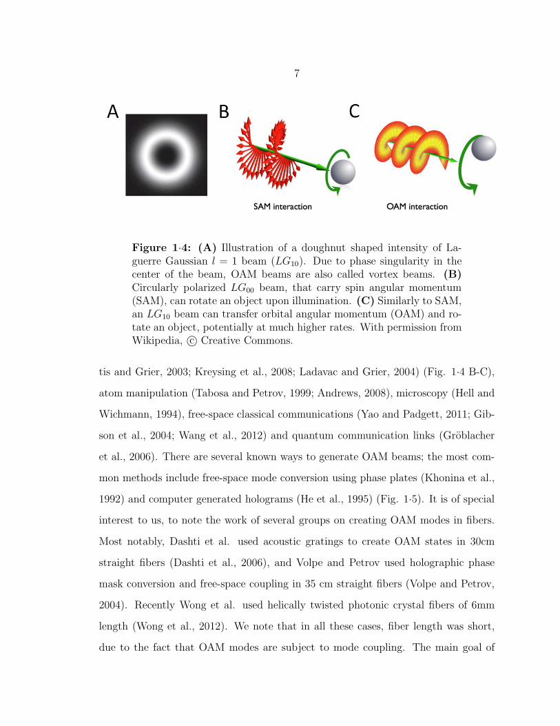
1·4 (A) Illustration of a doughnut shaped intensity of Laguerre Gaussian

l = 1 beam (LG10). Due to phase singularity in the center of the beam,

OAM beams are also called vortex beams. (B) Circularly polarized

LG00 beam, that carry spin angular momentum (SAM), can rotate

an object upon illumination. (C) Similarly to SAM, an LG10 beam

can transfer orbital angular momentum (OAM) and rotate an object,

potentially at much higher rates. With permission from Wikipedia, c©

Creative Commons. . . . . . . . . . . . . . . . . . . . . . . . . . . . . 7

xi

1·5 Example of conversion between fundamental Laguerre Gaussian (LG0m)

and higher order (LG1m) beam using a spiral phase plate with a phase

step equal to d = 2πlλ ≈ 10µm (for l = 1 and λ = 1550nm). With

permission from Wikipedia, c© Creative Commons. . . . . . . . . . . 8

1·6 (A) In this dissertation we study the idea of OAM as a new, orthog-

onal, degree of freedom in addition to wavelength, phase, amplitude

and polarization, for multiplexing in the future optical communication

systems. (B) OAM mode division multiplexing in fibers concept. . . 9

2·1 Numerical solutions for effective index, neff , for step index fiber, show-

ing labeling and corresponding values of l and m. . . . . . . . . . . . 16

2·2 First six modes (l = 0 and l = 1 groups) in a step index fiber. . . . . 16

2·3 Intensity patterns of the first-order mode group in vortex fiber. Ar-

rows show the polarization of the electric field. The top row shows

vector modes that are the exact vector solutions of the Eq. 2.18, while

the bottom row shows the resultant, unstable LP11 modes commonly

obtained at a fiber output. Specific linear combinations of pairs of top

row of modes, resulting in the variety of LP11 modes obtained at a

fiber output, are shown by colored lines (Ramachandran et al., 2009).

With permission from (Ramachandran et al., 2009). c© OSA. . . . . . 23

2·4 Concept of effective index separation in the first-order modes (A) Typ-

ical step-index MMF does not exhibit effective index separation caus-

ing mode coupling. (B) neff separation caused by desired fiber index

profile. . . . . . . . . . . . . . . . . . . . . . . . . . . . . . . . . . . . 24

3·1 (A) An optical microscope image of the end facet of the vortex fiber

dk11OD100. (B) Measured fiber refractive index for the dk11OD100

and dk11OD160. . . . . . . . . . . . . . . . . . . . . . . . . . . . . . 28

xii

3·2 Comparison of the simulated fields using scalar and vector numerical

method for the dk11OD105 fiber case. . . . . . . . . . . . . . . . . . 29

3·3 Numerically calculated properties of the dk11OD105 vortex fiber. Sep-

aration of neff indicates potential for smaller mode coupling (A-B).

Mode profiles in 1D and 2D case (C-D), latter obtained from the 1D

profiles assuming circular symmetry. Polarization at certain points can

be also obtained assuming azimuthal dependence of the modes (Table

2.3). . . . . . . . . . . . . . . . . . . . . . . . . . . . . . . . . . . . . 30

3·4 (A) Effective indices for guided modes for the dk11OD160 vortex fiber.

(B) Corresponding LP notation designating certain groups of modes. 31

3·5 Effective index difference (also called mode separation) versus fiber OD

between different modes. . . . . . . . . . . . . . . . . . . . . . . . . . 32

3·6 Table of guided modes for different OD fibers, at 1550nm. OD105

offers largest diameter fiber for which l ≥ 2 modes are cuts off. . . . . 32

3·7 Numerically calculated properties of the dk11OD105 vortex fiber . . . 33

3·8 Measured and numerically calculated ∆neff with respect to the HE11

mode for (A) OD100, (B) OD110 and (C) OD115 vortex fibers. . . . 33

3·9 Group index difference among HE11 and HE21 vortex fiber modes for

several different OD. . . . . . . . . . . . . . . . . . . . . . . . . . . . 34

3·10 Transmission power difference (in dB) between HE21 and HE11 modes

showing linear dependence of the loss in length. Gradient of the fit 0.33

dB/km gives the excess (i.e. differential) loss between the two modes. 35

3·11 Setup for OAM mode imaging. This setup enables us to measure both

the intensity and the phase of the beam. . . . . . . . . . . . . . . . . 36

xiii

3·12 (A) OAM mode intensity profile and (B) a line profile along the ring.

(C,D) Observed interference patterns between the OAM mode and

the reference beam when the two beams are (C) collinear or (D) form

an angle . (E,F) Simulated interference patterns in the two cases. . . 37

3·13 Comparison of the simulated and imaged mode profiles for OD100

case. . . . . . . . . . . . . . . . . . . . . . . . . . . . . . . . . . . . . 38

4·1 Microbend gratings. (A) Mode conversion setup. (B) Picture of the

microbend grating. (C) Effective indices of modes supported by the

vortex fiber (also see 3·8). Microbend grating period can be tuned to

allow for mode conversion from HE11 to first-order modes (denoted by

arrows). . . . . . . . . . . . . . . . . . . . . . . . . . . . . . . . . . . 43

4·2 Microbend resonance characteristic with respect to input polarization,

grating length and fiber roll angle. (A) Polarization dependence. (B)

HE21 resonances for different grating lengths. Longer grating length

require less pressure per fiber length, hence, pressure induced splitting

is smaller. Note grating bandwidth change with length, in agreement

with the theory. (C) Microbend pressure for HEodd21 and HEeven

21 reso-

nances vs fiber roll angle (i.e. rotation axis is along the fiber). . . . . 45

4·3 CO2 laser induced gratings. (A) Setup. Laser beam is focused onto the

fiber and point-to-point grating is written onto the vortex fiber. (B)

Setup photo (blue line indicates beam path, red line indicates vortex

fiber). (C) Microscope image of the grating inscribed in the fiber,

indicating periodic mechanical changes. (D) Polarization dependence

of the CO2 gratings. In comparison to microbend gratings (Fig. 4·2),

CO2 gratings are less polarization sensitive. . . . . . . . . . . . . . . 47

xiv

4·4 (A) Tension and fiber width profile for a 5-5-5µm taper geometry with

40µm waist. (B) Resonance for dk11OD100 fiber in the case of a taper

shown in A. . . . . . . . . . . . . . . . . . . . . . . . . . . . . . . . . 51

4·5 Loss transmission spectrum for HE11 and HE21 phase matched case.

Fitting the curve with the expected sinc2 profile gives the group index

difference ∆ng. . . . . . . . . . . . . . . . . . . . . . . . . . . . . . . 53

4·6 Phase matching curves Λ(λ) relate grating period Λ with resonant

wavelength (particular example is for the case of dk110127OD100 fiber).

Respective ∆neff and ∆ng can be calculated (bottom two graphs). . 54

4·7 (A) SLM mode conversion concept. After reflection off a SLM, an

OAM beam is created. (B) The spiral SLM pattern that creates the

LG10 beam at the same reflection angle as the LG00 beam incident

angle. (C) The fork SLM pattern that creates the LG10 beam at the

different reflection angle from the LG00 beam incident angle. . . . . . 55

4·8 Spatial light modulator based mode conversion. (A) Setup. (B) Photo

of the setup. . . . . . . . . . . . . . . . . . . . . . . . . . . . . . . . . 56

4·9 Spiral and fork holograms that create LG∗10, showing the effect of tilt

in the case of the fork hologram. . . . . . . . . . . . . . . . . . . . . . 56

4·10 Back-reflection from the mirror installed instead of the fiber for three

different axial positions of the coupling stage for a beam free of aberra-

tions: (A,C) defocused LG00 (B) focused LG00 (D,F) defocused LG10

(OAM mode)(E) focused LG10. Symmetric pattern, indicates good

alignment between input beam and the fiber. . . . . . . . . . . . . . . 57

xv

4·11 Camera image at the CamPos1 for the vortex fiber installed. Donut

mode represents back reflection from the fiber end-face (similar to the

case of the mirror in the Fig. 4·10). HE11 mode represents light coming

out of the vortex fiber, when the other fiber end is connected to the

light source. Two images here are intentionally misaligned. . . . . . . 57

4·12 Output of the vortex fiber after OAM mode coupling. (A) Aligned

and (B) misaligned case. . . . . . . . . . . . . . . . . . . . . . . . . . 58

5·1 Setup for imaging vortex fiber output. (A) Experimental setup that

uses grating for OAM mode generation. (B) Grating resonance spec-

trum used to deduce HEo21 mode conversion level. (C) Camera image

of the four polarization projections of the fiber output. Acronyms: left

circular (LC), right circular (RC), vertical (V) and horizontal (H), non-

polarizing beam splitter (NPBS), quarter wave plate (QWP), polariz-

ing beam displacing prism (PBDP). Vertical (V) polarization projec-

tion was interfered with the reference beam (Ref.) in order to observe

the phase of the vortex beam. Showed is the l = +1 OAM state that

is circularly polarized (spin = 1). . . . . . . . . . . . . . . . . . . . . 60

5·2 Camera images for the three positions of the polcon2 paddles, tuned

to achieve (A) l = 1, (B) l = 0 and (C) l = −1 state. . . . . . . . . 62

5·3 Ring method analysis for determining modal content of the vortex

fiber. (A) Azimuthal intensity profile of LC projection for radius r0.

(B) Fourier series coefficients for profile in (A). (C) Extracted modal

power contributions. . . . . . . . . . . . . . . . . . . . . . . . . . . . 64

xvi

5·4 Ring method analysis applied in real time. (A) Mode powers in time

during continuous adjustment of the paddles of PolCon2 (on the vortex

fiber) to obtain desired OAM state superposition. (B) Camera images

of the three positions (a-c). . . . . . . . . . . . . . . . . . . . . . . . . 66

5·5 Ring method error estimation. (A) Random simulated image created

as an weighted average of the six modes V +,−21 V +,−

T and V +,−11 with

randomized phases (dark and shot noise were also accounted for). (B-

D) Estimated modal power error with respect to different initial modal

powers for (B) V +21 , (C) V

+T and (D) V +

11 modes. We see that errors on

average increase as input powers of spurious modes increase, indicating

that the assumed ’dominant mode model’ is no longer valid. For this

reason calculations were only done for powers < −5dB with respect to

total power. . . . . . . . . . . . . . . . . . . . . . . . . . . . . . . . . 67

5·6 (A) Concept of higher-order Poincare sphere (taken with permission

from (Milione et al., 2011)). (B) Reconstruction of a relative phase

between two OAM states for the same case of tuning OAM shown in

Fig. 5·4. . . . . . . . . . . . . . . . . . . . . . . . . . . . . . . . . . . 68

5·7 (A-C) Relative mode powers for three different lengths for the case

of high purity (> 21dB) OAM+ mode excitation at 1550 nm (OAM

power refers to combined OAM+ and OAM− mode powers, and LP01

refers to combined powers of the two LP±

01 states). (D) Measured

modal power ratios as a function of fiber length for the same case as

in A-C. (E) Relative mode powers with respect to time, showing the

temporal stability of the OAM modes. . . . . . . . . . . . . . . . . . 70

xvii

5·8 (A) Power fraction in the fundamental, transverse, and HE21 pairs;

(B) Power estimated in the HE11 modes by regression analysis (red

crosses) and by coupling into a SMF (blue curve). (C) Estimated

power fraction of each of the two OAM states; (D) Estimated relative

phase of the two OAM states. . . . . . . . . . . . . . . . . . . . . . . 72

6·1 OAM division multiplexing principle. Four modes with distinct val-

ues of OAM (l) and spin (s) values are multiplexed into a specialty

fiber, propagated and analyzed at the output using bit-error-rate tester

(BERT) and/or imaged using near-IR camera. . . . . . . . . . . . . . 74

6·2 Detailed (de) multiplexing experimental setup: signal from the trans-

mitter (Tx) is split into four individual fiber arms. Two of the arms

were converted into OAM modes using LCoS-SLM. Two fundamental

modes were added collinearly to the two OAM modes using 3dB-loosy

non-polarizing beam-splitter. All four modes are then coupled into

vortex fiber, and analyzed at the output after being demultiplexed

accordingly. Acronyms: flip mirror (FM), half wave plate (HWP),

(non)-polarizing beam-splitter ((N)PBS), polarization beam combiner

(PBC), polarization controller (PC), mirror (M), quarter wave plate

(QWP). . . . . . . . . . . . . . . . . . . . . . . . . . . . . . . . . . . 75

6·3 NIR camera images of the channel outputs after 1.1km fiber propa-

gation using 50GBaud modulated ECL source (linewidth of 0.4nm).

(A-D) Intensity images (E, F) Phase images of OAM+ and OAM−.

(G, H) Intensity and phase of the OAM+ mode after demultiplexing

using inverse fork pattern. . . . . . . . . . . . . . . . . . . . . . . . . 77

xviii

6·4 Cross-talk and Multipath interference. (A) Cross-talk measurement

example (B) Example of the LP+01 mode power drift (attributed to the

cross-talk and free-space optics) and power fluctuations (due to mul-

tipath interference - MPI). (Inset) Cross talk and MPI mechanisms;

mode A can couple into mode B producing cross-talk, but certain

amount of the power can couple back into mode A interfering with

the original signal, producing MPI. Both cross-talk and MPI cause

higher BER. (C) Table of measured values for cross-talk and MPI for

all four modes. . . . . . . . . . . . . . . . . . . . . . . . . . . . . . . 78

6·5 Drift and MPI of all four modes. . . . . . . . . . . . . . . . . . . . . 79

7·1 Basic modulation formats using amplitude and phase od the field. Non-

return to zero (NRZ) denotes that signal doesn’t go to zero between

two bits that both carry ’1’. With permission from Wikipedia, c©

Creative Commons. . . . . . . . . . . . . . . . . . . . . . . . . . . . . 83

7·2 Advanced modulation formats (Winzer and Essiambre, 2006). For us

most important formats is differential quadrature phase shift keying

(DQPSK) that we use in our systems experiment. For full list of

acronyms consult (Winzer and Essiambre, 2006). With permission

from (Winzer and Essiambre, 2006), c© IEEE. . . . . . . . . . . . . . 84

7·3 Direct (A) vs Coherent (B) modulation formats. With permission from

Wikipedia, c© Creative Commons. . . . . . . . . . . . . . . . . . . . . 84

xix

7·4 Concept of quadrature phase shift keying (QPSK) and eye-diagram for

bit-error-rate testing. (A) Ideal QPSK constellation. A sender can

encode information in a π/4, +3π/4, 5π/4 and +7π/4 phase, corre-

sponding to 11, 01, 00 and 11 bit combination. Therefore, a phase can

carry 4 possible states. (B) Noisy case. A phase of light can suffer

changes due to fiber impediments, and in the noisy case, wrong phase

can be detected, and errors in transmission can occur. (C) Concept

of an eye diagram in the case of intensity modulation. Train of pulses

carrying bits can be overlapped to create an eye-shaped diagram. (C)

In a noisy case, distortion can cause ”eye-closing” introducing errors in

transmission. Similar eye diagram can be observed in the QPSK case.

C and D with permission from Wikipedia, c© Creative Commons . . . 86

xx

7·5 Systems experiment setup: signal from the laser or WDM source is mod-

ulated, amplified using an erbium doped fiber amplifier (EDFA), filtered

using a band pass filter (BPF) and split into four individual fiber arms (two

in the case of the WDM experiment). Two of the arms were converted

into OAM modes using the input SLM. Two fundamental modes were also

collinearly aligned with the two OAM modes using a beam-splitter, and

all four modes were coupled into the fiber. After propagation, the modes

are demultiplexed sequentially and sent for coherent detection and offline

digital signal processing (DSP). Acronyms: ADC - analog digital conver-

tor, Att - attenuator, FM - flip mirror, LO - local oscillator, OC - optical

coupler, (N)PBS: (non)-polarizing beam-splitter, PBC - polarization beam

combiner, PC - polarization controllers, PC-SMF - polarization controller on

SMF, PC-VF - polarization controller on vortex fiber. OC: optical coupler,

(N)PBS: (non)-polarizing beam-splitter, PBC: polarization beam combiner,

PC: polarization controller . . . . . . . . . . . . . . . . . . . . . . . . . 88

7·6 Constellation diagrams in the case of 4-mode OAM-MDM, with 50

GBaud NRZ-QPSK, λ = 1550nm, for the single-channel, and all-

channel cases. Note the larger distortion of the constellations in the

all-channel case. . . . . . . . . . . . . . . . . . . . . . . . . . . . . . . 90

7·7 Data transmission experiments. (A) Block diagram of 50 × 2 Gb/s

QPSK signal transmission over a single wavelength carrying 4 modes

in the vortex fiber. (B) Measured BER as a function of received power

for the single-channel (SC) and all-channels (AC) transmission case. . 91

xxi

7·8 (A) Block diagram of 20×4 Gb/s 16-QAM signal transmission over

10 wavelengths carrying 2 modes in the vortex fiber. (B) Measured

crosstalk between OAM± modes as a function of wavelength. (C)

BER as a function of wavelength for OAM± modes in the WDM

system. . . . . . . . . . . . . . . . . . . . . . . . . . . . . . . . . . . . 92

7·9 Additional experimental results of the 2-OAM modes, 10 wavelengths,

16-QAM systems experiments. (A) Spectrum of the modulated signal

at the output of the WDM 16-QAM Tx, and spectrum of the OAM+

mode at the receiver after demultiplexing. (B) Constellations of 16-

QAM modulation for the demultiplexed OAM+ mode at 1550.64 nm,

for several cases (without and with crosstalk). (C) BER as a function

of received power at 1550.64 nm, for B2B, and OAM modes without

and with XT from WDM channels or the other OAM mode. . . . . . 93

7·10 Spiral interference patterns, showing helical phase, of the OAM+ mode

at different wavelengths for the same vortex fiber conditions (no polar-

ization controller adjustments). (A-D) Spiral patterns for the wave-

lengths spaced in 10pm, 100pm, and 1000pm. (E-H) Spirals for the

wavelengths spaced in 10nm. . . . . . . . . . . . . . . . . . . . . . . . 94

8·1 Setup to measure polarization dependence of a beamsplitter. . . . . . 102

8·2 Sample Newport 10BC17MB.1. Measured polarization after reflection

for three different positions of a polarizer: a) horizontal, b) vertical and

c) 45o degrees linearly polarized states, as well as after transmission of

a 45o degrees linearly polarized state (d). Clearly, phase delay between

polarizations is introduced in the case of a 45o degrees linearly polarized

state, especially in the reflection case. . . . . . . . . . . . . . . . . . . 103

xxii

8·3 Polarization after reflection of a 45o angled mirror (Thorlabs, BB1 −

E04). . . . . . . . . . . . . . . . . . . . . . . . . . . . . . . . . . . . . 103

8·4 Polarization after reflection from a beam-splitter (Thorlabs BS015) . 103

8·5 Schematic of experimental setup. Polarization-entangled photons (1550-

nm and 1558-nm) are sent in two different channels A and B. 1.1km

long channel A used two gratings to convert between fundamental and

OAM mode with > 80% efficiency. Channel B consisted of 5km long

single mode fiber (SMF); Time delay was tuned to target coincidence

of channel A photons (traveled in a fundamental mode) and channel

B photons (traveled in the OAM mode). Full quantum tomography

measurement was applied at the receivers’ end and density matrix of

photon pair was measured. . . . . . . . . . . . . . . . . . . . . . . . . 104

8·6 Resonances for the case of microbend only (right), CO2 only (center)

and both (left). . . . . . . . . . . . . . . . . . . . . . . . . . . . . . . 105

8·7 Measured density matrix, P-parameter, concurrence (C) and S-parame-

ter. . . . . . . . . . . . . . . . . . . . . . . . . . . . . . . . . . . . . . 105

xxiii

List of Abbreviations

AOF . . . . . . . . . . . . . adaptive optics feedbackBER . . . . . . . . . . . . . bit-error rateCCD . . . . . . . . . . . . . charged-coupled deviceCW . . . . . . . . . . . . . continuous waveDSP . . . . . . . . . . . . . digital signal processingDSF . . . . . . . . . . . . . dispersion shifter fiberECL . . . . . . . . . . . . . external cavity laserEDFA . . . . . . . . . . . . . Erbium-doped fiber amplifierFDE . . . . . . . . . . . . . frequency domain equalizationFFT . . . . . . . . . . . . . fast Fourier transformFM . . . . . . . . . . . . . flip-mirrorFWM . . . . . . . . . . . . . four-wave mixingFWHM . . . . . . . . . . . . . full-width at half maximumHOM . . . . . . . . . . . . . higher-order-modeGD . . . . . . . . . . . . . group delayITU . . . . . . . . . . . . . International Telecommunications UnionIEEE . . . . . . . . . . . . . Institute of Electrical and Electronics EngineersLAN . . . . . . . . . . . . . local-area networkLCoS . . . . . . . . . . . . . liquid crystal on siliconLG . . . . . . . . . . . . . Laguerre-GaussianLO . . . . . . . . . . . . . local oscillatorMD . . . . . . . . . . . . . mode dispersionMCF . . . . . . . . . . . . . multi-core fiberMDM . . . . . . . . . . . . . mode-division multiplexingMDL . . . . . . . . . . . . . mode dependant lossMIMO . . . . . . . . . . . . . multiple-input multiple-outputMMF . . . . . . . . . . . . . multi-mode fiber

xxiv

OAM . . . . . . . . . . . . . orbital angular momentumOD . . . . . . . . . . . . . outer diameterOFDE . . . . . . . . . . . . . orthogonal frequency domain multiplexingOOK . . . . . . . . . . . . . on-off-keyingOSA . . . . . . . . . . . . . optical spectrum analyzerPDM . . . . . . . . . . . . . polarization-division-multiplexingPIC . . . . . . . . . . . . . photonic integrated circuitPSK . . . . . . . . . . . . . phase-shift-keyingQAM . . . . . . . . . . . . . quadrature-amplitude-modulationQPSK . . . . . . . . . . . . . quadrature-phase-shift-keyingSE . . . . . . . . . . . . . spectral-efficiencySDM . . . . . . . . . . . . . space-division-multiplexingSLM . . . . . . . . . . . . . spatial-light-modulatorSMF . . . . . . . . . . . . . single mode fiberSNR . . . . . . . . . . . . . signal-to-noise-ratioTDE . . . . . . . . . . . . . time-domain equalizationTE . . . . . . . . . . . . . transverse electricTM . . . . . . . . . . . . . transverse magneticWDM . . . . . . . . . . . . . wavelength-division-multiplexingWGA . . . . . . . . . . . . . weakly-guided approximation

xxv

1

Chapter 1

Introduction

1.1 Optical fiber communications and space-division multi-

plexing

Optical communication network traffic has been steadily increasing by a factor of

100 every decade, with the capacity of single-mode optical fiber increasing 10’000

times in the last three decades (Essiambre and Tkach, 2012) (Fig. 1·1). Historically,

this growth has been sustained by information multiplexing techniques using wave-

length, amplitude, phase and polarization of light as means to encode information

(Agrawal, 2010). Several major discoveries in the fiber optics domain enabled the

today’s optical networks. The first one was led by Charles M. Kao ground-breaking

work that recognized glass impurities as the major loss mechanism (at the time bulk

glass loss was ≈ 200dB/km at 1µm) (Kao and Hockham, 1966). This work gave the

birth to optical fibers and led to the first commercial fibers in the 1970 with attenu-

ation low enough for communication purposes (≈ 20dB/km). Development of single

mode fibers (SMF) in the early 80’s reduced pulse dispersion and lead to the first

fiber-optic based transatlantic telephone cables. Development of Indium Gallium Ar-

senide photodiode in the early 90’s shifted the focus to the near infrared wavelengths

(1550nm), where silica has the lowest loss, enabling extended reach. At roughly

the same time, the invention of erbium-doped fiber amplifiers resulted in one of the

biggest leaps in fiber capacity in the history of communications, a 1000-fold increase

in capacity in 10 years (Fig. 1·1 B). The improvement was mainly due to removed

2

need for expensive repeaters for signal regeneration, as well as efficient amplification

of many wavelengths at the same time, enabling wavelength-division-multiplexing

(WDM). Throughout the 2000s, bandwidth increase came mainly from introduction

of complex signal modulation formats and coherent detection, allowing information

encoding using the phase of light. Most recently, polarization-division-multiplexing

(PDM) doubled the channel capacity (Fig. 1·1 A-B).

Figure 1·1: (A) North American Internet traffic in Petabytes/monthaccording to several studies, such as Minnesota Internet Traffic Study(MINTS) and Cisco. (Essiambre and Tkach, 2012).(B) Capacity evo-lution for different communication systems (Sakaguchi et al., 2012).With permission from (Essiambre and Tkach, 2012) and (Sakaguchiet al., 2012), c© IEEE.

Though fiber communications based on SMFs featured tremendous growth in

the last three decades, recent research has indicated SMF limitations. Nonlinear

effects in silica play a significant role in long-range transmission, mainly through Kerr

effect, where a presence of a channel at one wavelength can change the refractive

index of a fiber, causing distortions of other wavelength channels (Marcuse et al.,

1991). Recently, a spectral efficiency (SE) (or bandwidth efficiency), referring to the

transmitted information rate over a given bandwidth, has been theoretically analyzed

assuming nonlinear effects in a noisy fiber channel (Essiambre et al., 2010). This

3

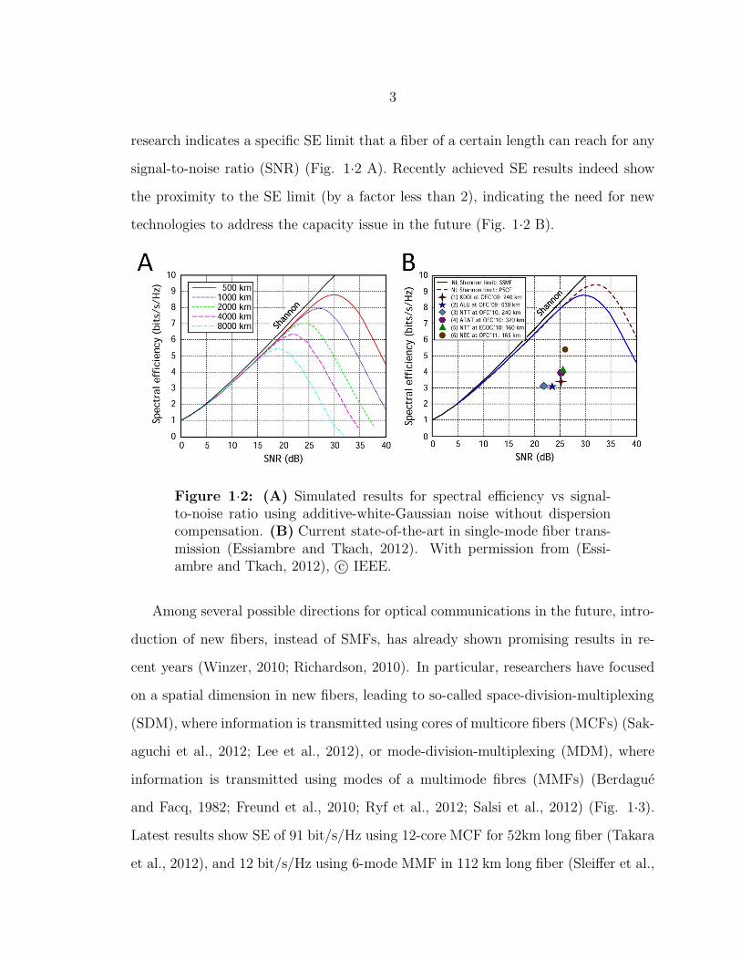
research indicates a specific SE limit that a fiber of a certain length can reach for any

signal-to-noise ratio (SNR) (Fig. 1·2 A). Recently achieved SE results indeed show

the proximity to the SE limit (by a factor less than 2), indicating the need for new

technologies to address the capacity issue in the future (Fig. 1·2 B).

Figure 1·2: (A) Simulated results for spectral efficiency vs signal-to-noise ratio using additive-white-Gaussian noise without dispersioncompensation. (B) Current state-of-the-art in single-mode fiber trans-mission (Essiambre and Tkach, 2012). With permission from (Essi-ambre and Tkach, 2012), c© IEEE.

Among several possible directions for optical communications in the future, intro-

duction of new fibers, instead of SMFs, has already shown promising results in re-

cent years (Winzer, 2010; Richardson, 2010). In particular, researchers have focused

on a spatial dimension in new fibers, leading to so-called space-division-multiplexing

(SDM), where information is transmitted using cores of multicore fibers (MCFs) (Sak-

aguchi et al., 2012; Lee et al., 2012), or mode-division-multiplexing (MDM), where

information is transmitted using modes of a multimode fibres (MMFs) (Berdague

and Facq, 1982; Freund et al., 2010; Ryf et al., 2012; Salsi et al., 2012) (Fig. 1·3).

Latest results show SE of 91 bit/s/Hz using 12-core MCF for 52km long fiber (Takara

et al., 2012), and 12 bit/s/Hz using 6-mode MMF in 112 km long fiber (Sleiffer et al.,

4

2012) (compare with Fig. 1·2 A for SMF). Somewhat unconventional transmission

at 2.08 µm has also been demonstrated in 290m-long photonic crystal fibers, though

still with high losses (4.5 dB/km) (Petrovich et al., 2012).

Figure 1·3: Different types of fibers considered for future communica-tion links in order to increase network capacity (Essiambre and Tkach,2012). With permission from (Essiambre and Tkach, 2012), c© IEEE.

While offering promising results, these new types of fibers have their own limita-

tions. Being non-circularly symmetric structures, MCFs are known to require more

complex, expensive manufacturing. On the other hand, MMFs are easily created us-

ing existing technologies (Wang et al., 2006), however, conventional MMF systems are

known to suffer from mode coupling caused by both random perturbations in fibers

(Gloge, 1972; Marcuse, 1974) and in modal (de)multiplexers (Ryf et al., 2012). Sev-

eral techniques can be used for mitigating mode coupling. In a strong-coupling regime

(typically >km), modal crosstalk must be compensated using computationally inten-

5

sive multiple-input multiple-output (MIMO) digital signal processing (DSP) (Stuart,

2000; Randel et al., 2011). While MIMO DSP leverages the technique’s current suc-

cess in wireless networks (Foschini and Gans, 1998)1, the wireless networks data rates

are several orders of magnitude lower then ones required for optical networks. Fur-

thermore, MIMO DSP complexity inevitably increases with an increasing number of

modes (Arik et al., 2013) and no MIMO-based data transmission demonstrations have

been demonstrated in real time so far. Furthermore, unlike wireless communication

systems, optical systems are further complicated because of fiber nonlinear effects

(Essiambre and Tkach, 2012). In a weak-coupling regime (typically <km) where

cross-talk is smaller, methods that also use computationally intensive adaptive optics

feedback algorithms have been demonstrated (Panicker and Kahn, 2009; Carpenter

and Wilkinson, 2012b). These methods ”reverse” the effect of mode coupling by

sending a desired superposition of modes at the input, so that desired output mode

can be obtained. This approach is limited however, since mode coupling is a random

process that can change on the order of a millisecond in conventional fibers ((Ho and

Kahn, 2013) p. 40). Therefore, the adaptation of this method can be problematic

in long-haul systems, where the round-trip signal propagation delay can be tens of

milliseconds. Though 2× 56Gb/s transmission at 8km length has been demonstrated

in the case of two higher order modes (Carpenter et al., 2013), none of the adaptive

optics MDM methods to date have been demonstrated for more than two modes.

In this dissertation we introduce a new possibility for future network capacity

increase, using a special class of MMFs capable of reducing mode coupling. This new

type of fibers allows for propagation of so-called orbital angular momentum (OAM)

fiber modes. Regarding the MIMO-based MDM and adaptive optics techniques that

we mentioned, our approach offers two potential advantages: 1) by using specially de-

signed optical fibers to reduce mode coupling, the computational complexity required

1MIMO DSP was introduced in 4G wireless networks

6

on the electronic end can be reduced, and 2) because of the uniqueness of OAM

modes over other basis sets (that we’ll explore more in details), these modes offer

theoretically lossless ways of multiplexing into fibers (Berkhout et al., 2010; Sullivan

et al., 2012; Su et al., 2012; Cai et al., 2012). Before we go further into details of the

method we propose here, we first introduce the orbital angular momentum of light.

1.2 Orbital angular momentum (OAM) of light

Together with energy and momentum, angular momentum is one of the most fun-

damental physical quantities in classical and quantum electrodynamics (Mandel and

Wolf, 1995). In a vacuum, electromagnetic angular momentum is defined as:

~M def

= ǫ0~r × (~E × ~B)

where ~E and ~B are electrical and magnetic fields, and ǫ0 is the vacuum electric per-

mittivity. In paraxial beams, angular momentum can be divided into spin angular

momentum (SAM) and orbital angular momentum (OAM) (Jackson, 1962). SAM

is associated with photon spin and is manifested as circular polarization (Poynting,

1909; Beth, 1936). In contrast, OAM is linked to the spatial distribution of the electric

field (Jackson, 1962). In particular, beams with electric field proportional to exp(ilφ),

have the OAM of l~ per photon (Allen et al., 1992), where l is topological charge, φ

is azimuthal angle, and ~ is Planks constant h divided by 2π. Examples of the beams

that have non-zero OAM include free-space Laguerre-Gaussian beams (LGlm modes

with l 6= 0), as well as Bessel beams, Mathieu beams, and Ince-Gaussian beams (Fig.

1·4 A). Due to their phase singularity in the center of the beam, OAM carrying beams

(or simply OAM beams) are also called vortex beams or optical vortices.

Since their first lab demonstration (Allen et al., 1992), OAM beams achieved a

widespread scientific and technological interest in the areas of optical tweezers (Cur-

7

Figure 1·4: (A) Illustration of a doughnut shaped intensity of La-guerre Gaussian l = 1 beam (LG10). Due to phase singularity in thecenter of the beam, OAM beams are also called vortex beams. (B)Circularly polarized LG00 beam, that carry spin angular momentum(SAM), can rotate an object upon illumination. (C) Similarly to SAM,an LG10 beam can transfer orbital angular momentum (OAM) and ro-tate an object, potentially at much higher rates. With permission fromWikipedia, c© Creative Commons.

tis and Grier, 2003; Kreysing et al., 2008; Ladavac and Grier, 2004) (Fig. 1·4 B-C),

atom manipulation (Tabosa and Petrov, 1999; Andrews, 2008), microscopy (Hell and

Wichmann, 1994), free-space classical communications (Yao and Padgett, 2011; Gib-

son et al., 2004; Wang et al., 2012) and quantum communication links (Groblacher

et al., 2006). There are several known ways to generate OAM beams; the most com-

mon methods include free-space mode conversion using phase plates (Khonina et al.,

1992) and computer generated holograms (He et al., 1995) (Fig. 1·5). It is of special

interest to us, to note the work of several groups on creating OAM modes in fibers.

Most notably, Dashti et al. used acoustic gratings to create OAM states in 30cm

straight fibers (Dashti et al., 2006), and Volpe and Petrov used holographic phase

mask conversion and free-space coupling in 35 cm straight fibers (Volpe and Petrov,

2004). Recently Wong et al. used helically twisted photonic crystal fibers of 6mm

length (Wong et al., 2012). We note that in all these cases, fiber length was short,

due to the fact that OAM modes are subject to mode coupling. The main goal of

8

Figure 1·5: Example of conversion between fundamental LaguerreGaussian (LG0m) and higher order (LG1m) beam using a spiral phaseplate with a phase step equal to d = 2πlλ ≈ 10µm (for l = 1 and λ =1550nm). With permission from Wikipedia, c© Creative Commons.

this dissertation is to study whether a special class of fibers can overcome this prob-

lem of mode coupling, allowing OAM mode propagation for longer fiber lengths. If

OAM mode stability is feasible in fibers, data streams could be, in principle, sent us-

ing independent fiber OAM modes. This concept of OAM mode-division-multiplexing

(OAM-MDM) has been previously used in free-space where several classical and quan-

tum communications experiments have exploited this inherent orthogonality of OAM

modes (Gibson et al., 2004; Groblacher et al., 2006; Wang et al., 2012). This disser-

tation aims to address the possibility of fiber-based OAM-MDM, as a way of capacity

increase in future fiber based systems (Fig. 1·6).

We start this study by mathematical description of MMFs using electromagnetic

theory (Ch. 2). We introduce OAM fiber modes and discuss the parameters necessary

for their stability. In chapter 3, we study the properties of a special type of fibers,

called vortex fibers, using numerical and experimental methods. We observe that vor-

tex fibers indicate reduce mode coupling and we verify the existence of OAM modes

qualitatively. In chapter 4, we address OAM mode generation in vortex fibers using

methods based on fiber gratings and spatial light modulators (SLMs), both methods

used for results presented in subsequent chapters. In chapter 5 we study two meth-

9

Figure 1·6: (A) In this dissertation we study the idea of OAM as anew, orthogonal, degree of freedom in addition to wavelength, phase,amplitude and polarization, for multiplexing in the future optical com-munication systems. (B) OAM mode division multiplexing in fibersconcept.

ods for determining purity of OAM modes: the ring technique and the regression

method. Using these methods we address the OAM mode evolution for different fiber

lengths. In Chapter 6 we study how to excite several OAM modes simultaneously to

achieve OAM-MDM. We describe a 4-mode multiplexing and demultiplexing system

of two fundamental and two l = ±1 modes using free space optics and spatial light

modulators. Finally, in chapter 7 we present the results of data transmission exper-

iments using four aforementioned modes to achieve data transmission at 400 Gbit/s

using four OAM modes, at a single wavelength, and 1.6Tbit/s using two OAM modes

and 10 wavelengths. In chapter 8, we discuss some of the limitations of OAM-MDM

method, and speculate future directions.

10

Chapter 2

Multimode Fibers and Mode Stability

In this chapter we first use electromagnetic theory to derive solutions for multimode

fiber waveguides (also called modes) in a weakly guided approximation. We then

shown that certain fiber modes have non-zero OAM of topological charge l (hence

the name OAM modes). Similarly to the free-space LGlm modes, these OAM modes

have a helical phase of electric field proportional to exp(ilφ) and as we will see, the

crucial factor for this is an existence of non-zero azimuthal component of a Poynting

vector. At the end of the chapter, we discuss the necessary conditions for these OAM

states to be stable in fibers, and the role of fiber mode coupling which in general case

restricts a long-range OAM mode fiber propagation.

2.1 Optical fiber waveguide theory

Optical fibers waveguide theory has been well studied in literature (Saleh and Teich,

2007; Iizuka, 2002; Snyder and Love, 1983). In an ideal case, optical fibers are 2D

cylindrical waveguides comprising one (or several) cores surrounded by a cladding

having slightly lower refractive index (we assume no changes across longitudinal di-

mension of a fiber). A fiber mode is a solution (also known as eigenstate) of a

waveguide equation describing the field distribution that propagates in a fiber with-

out changing, except for the scaling factor. All fibers have a limit on the number

of modes that they can be propagating (denoted as N), and we include both spatial

and polarization degree of freedom. SMFs support propagation of two orthogonal

11

polarizations of the fundamental mode only (N=2), while for sufficiently large core

radius and/or the core-cladding difference, a fiber is multimoded (N > 2). Here, we

are mostly interested in a subset of multimode fibers that are weakly guided, meaning

that the core-cladding refractive index difference can be considered to be very small.

Most glass fibers made today are weakly guided with the exception of some photonic

crystal fibers and air-core fibers. We’ll show that a step-index fibers guide modes in

groups, where within each group modes typically have similar properties in terms of

effective index. Within a group the modes are said to be degenerate. However, as

we’ll see, these degeneracies can be broken in a certain fiber profile design.

We now look into mathematical description of the modes. In our derivation we

follow (Snyder and Love, 1983). We start by describing translationally invariant

waveguide with refractive index n = n(x, y), with nco being maximum refractive

index (typically in the ”core” of a waveguide), and ncl being refractive index of the

uniform cladding, and ρ represents the maximum radius of the refractive index n.

Due to translational invariance the solutions (or modes) for this waveguide, that we

are looking to find, can be written as:

Ej(x, y, z) = ej(x, y)eiβjz, (2.1)

Hj(x, y, z) = hj(x, y)eiβjz, (2.2)

where βj is called propagation constant of the j-th mode. Vector wave equation for

source free Maxwell’s equation can be written in this case as:

(∇2t + n2k2 − β2

j )ej = −(∇t + iβj z)(etj · ∇tln(n2)), (2.3)

(∇2t + n2k2 − β2

j )hj = −(∇tln(n2))× ((∇t + iβj z)× hj), (2.4)

where k = 2π/λ is the free-space wavenumber, λ is a free-space wavelength, et =

exx + eyy is a transverse part of the electric field, ∇2t is a transverse Laplacian and

12

∇t transverse vector gradient operator. Waveguide polarization properties are built

into the wave equation through the ∇tln(n2) terms and ignoring them would lead

to the scalar wave equation, with linearly polarized modes. We define profile height

parameter ∆, waveguide or fiber parameter V and modal parameters Uj and Wj as:

∆def

=1

2

(1− n2

cl

n2co

), (2.5)

Vdef

=2πρ

λ(n2

co − n2cl)

1/2, (2.6)

Ujdef

= ρ(k2n2co − b2j )

1/2, (2.7)

Wjdef

= ρ(b2j − k2n2cl)

1/2, (2.8)

where V 2 = U2j +W 2

j .

While previous equations satisfy arbitrary waveguide profile n(x, y), in most cases

of interest, profile height parameter ∆ can be considered small ∆ ≪ 1, in which case

waveguide is said to be weakly guided, or that weakly guided approximation (WGA)

holds. If this is the case, a perturbation theory can be applied to approximate the

solutions (Eq. 2.1) as:

E(x, y, z) = e(x, y)ei(β+β)z = (et + zez)ei(β+β)z (2.9)

H(x, y, z) = h(x, y)ei(β+β)z = (ht + zhz)ei(β+β)z, (2.10)

where subscripts t and z denote transverse and longitudinal components respectively.

Longitudinal components can be considered much smaller in WGA and we can ap-

proximate (but not neglect) them as:

ez =i(2∆)1/2

V(ρ∇t · et) (2.11)

hz =i(2∆)1/2

V(ρ∇t · ht) (2.12)

13

and transversal components satisfy the simplified wave equation:

(∇2t + n2k2 − β2

j )ej = 0, (2.13)

ht = nco

(ǫ0µ0

)1/2

z× et. (2.14)

We can write the polarization correction δβ as:

δβ =(2∆)3/2

2ρV

∫A(ρ∇t · et)et · ρ∇tfdA∫

Ae2tdA

, (2.15)

and delta can be approximated as ∆ ∼= nco−ncl

nco, and V parameter as:

V = kρnco

√n2co − n2

cl = kρnco(2∆)1/2. (2.16)

Though WGA simplified the waveguide equation, further simplification can be

obtained by assuming circularly symmetric waveguide (such as ideal fiber). If this is

the case refractive index that can be written as:

n(r) = n2co(1− 2f(R)∆) (2.17)

where f(R) ≥ 0 is our small arbitrary profile variation.

For a circularly symmetric waveguide, solving Eq. 2.13 can be simplified by the

separation of variables and the solutions (Eq. 2.9 and Eq. 2.10) will have propagation

constants βlm that are classified using azimuthal (l) and radial (m) numbers. Another

classification uses effective indices nlm (sometimes noted as nefflm or simply neff , that

are related to propagation constant as: βlm = knefflm ). For the case of l = 0, the

solutions can be separated into two classes that have either transverse electric (TE0m)

or transverse magnetic (TM0m) fields (so called meridional modes). In the case of

l 6= 0, both electric and magnetic field have z-component, and depending on which one

is more dominant, so-called hybrid modes are denoted as: HElm and EHlm. Complex

14

amplitudes for the two cases (l = 0, l ≥ 1), are given in the tables 2.1 - 2.3 (Snyder

and Love, 1983), where Fl represents solution of the Bessel equation:

[d2

dR2+

1

R

d

dR− l2

R2+ U2 − V 2f(R)

]Fl(R) = 0, (2.18)

and U , β (approximated U and β), and G±

l are defined as:

U2 def

= ρ(k2n2co − β2)1/2, (2.19)

βdef

= β + δβ, (2.20)

G±

l

def

=dFl

dR± l

RFl, (2.21)

where R = r/ρ is the normalized radius. We can also write simplified polarization

correction δβ in terms of two constituents, defined as (Snyder and Love, 1983):

I1def

=(2∆)3/2

4ρV

∫∞

0RFl(dFl/dR)(df/dR)dR∫

∞

0RF 2

l dR(2.22)

I2def

=l(2∆)3/2

4ρV

∫∞

0F 2l (df/dR)dR∫∞

0RF 2

l dR. (2.23)

Note that polarization correction δβ has different values within the same group of

modes with the same orbital number (l), even in the circularly symmetric fiber (col-

umn δβ in 2.3). This is an important observation that led to development of a special

type of fiber that we discuss in Ch. 3.

Mode et ht ez hz δβ

Even HE1m xF0 nco

(ǫ0µ0

)1/2

yF0 i(2∆)1/2

V G0cosφ inco

(ǫ0µ0

)1/2(2∆)1/2

V G0sinφ I1

Odd HE1m yF0 −nco

(ǫ0µ0

)1/2

xF0 i(2∆)1/2

V G0sinφ −inco

(ǫ0µ0

)1/2(2∆)1/2

V G0cosφ I1

Table 2.1: Fundamental HE11 and HE1m modes (l = 0). With per-mission from (Snyder and Love, 1983) c© Chapman and Hall.

15

Mode et ht

Even HEl+1,m (xcos lφ− ysin lφ)F1 nco

(ǫ0µ0

)1/2

(xsin lφ+ ycos lφ)Fl

TM0m(l = 1) (xcos lφ+ ysin lφ)Fl −nco

(ǫ0µ0

)1/2

(xsin lφ− ycos lφ)F1

Even EHl−1,m(l > 1) (xcos lφ+ ysin lφ)Fl −nco

(ǫ0µ0

)1/2

(xsin lφ− ycos lφ)Fl

Odd HEl+1,m (xsin lφ+ ycos lφ)Fl −nco

(ǫ0µ0

)1/2

(xcos lφ− ysin lφ)Fl

TE0m(l = 1) (xsin lφ− ycos lφ)Fl nco

(ǫ0µ0

)1/2

(xcos lφ+ ysin lφ)F1

Odd EHl−1,m(l ≥ 1) (xsin lφ− ycos lφ)Fl nco

(ǫ0µ0

)1/2

(xcos lφ+ ysin lφ)Fl

Table 2.2: Transversal components for higher-order modes (HOMs)(l ≥ 1 modes). With permission from (Snyder and Love, 1983) c©Chapman and Hall.

Mode ez hz δβ

Even HEl+1,m i(2∆)1/2

V G−

l cos(l + 1)φ inco

(ǫ0µ0

)1/2(2∆)1/2

V G−

l sin(l + 1)φ I1 − I2

TM0m(l = 1) i(2∆)1/2

V G+1 0 2(I1 + I2)

Even EHl−1,m(l > 1) i(2∆)1/2

V G+l cos(l − 1)φ −inco

(ǫ0µ0

)1/2(2∆)1/2

V G+l sin(l − 1)φ I1 + I2

Odd HEl+1,m i(2∆)1/2

V G−

l sin(l + 1)φ −inco

(ǫ0µ0

)1/2(2∆)1/2

V G−

l cos(l + 1)φ I1 − I2

TE0m(l = 1) 0 inco

(ǫ0µ0

)1/2(2∆)1/2

V G+1 0

Odd EHl−1,m(l ≥ 1) i(2∆)1/2

V G+l sin(l− 1)φ inco

(ǫ0µ0

)1/2(2∆)1/2

V G+l cos(l − 1)φ I1 + I2

Table 2.3: Longitudinal components for higher-order modes (l ≥ 1modes). With permission from (Snyder and Love, 1983) c© Chapmanand Hall.

In order to look more closely into mode properties, we choose step-index fiber as

an example, for which refractive index can be written as:

n(R) =

{nco, 0 ≤ R ≤ 1, core regionncl, 1 < R < ∞, cladding region

(2.24)

In this case, solutions to the Eq. 2.18 are the Bessel functions of the first kind, Jl(r),

in the core region, and modified Bessel functions of the second kind, Kl(r), in the

cladding region. Solutions for neff in the step-index case are shown on the Fig. 2·1.

16

1150 1200 1250 1300 1350 1400 1450 1500 1550

1.445

1.45

1.455

1.46

1.465

λ (nm)

n eff

HE11

TE0,1

HE21

TM0,1

EH11

HE31

HE13

HE14

TM0,2

HE22

TE0,2

HE32

EH22

HE41

nglass

Figure 2·1: Numerical solutions for effective index, neff , for step indexfiber, showing labeling and corresponding values of l and m.

In the case of step-index fiber the groups of modes are almost degenerate, also

meaning that the polarization correction δβ can be considered very small. Unlike

HE11 modes, higher order modes (HOMs) can have elaborate polarizations, and first

six modes (l = 0 and l = 1 groups) in a step index fiber are shown in Fig. 2·2.

We note that in the case of circularly symmetric fiber, the odd and even modes (for

example HEoddlm and HEeven

lm modes) are always degenerate (i.e. have equal neff ),

Figure 2·2: First six modes (l = 0 and l = 1 groups) in a step indexfiber.

17

regardless of the index profile (see the δβ column in the Table 2.3). These modes

will be non-degenerate only in the case of circularly asymmetric index profiles; an

example is polarization maintaining fiber (Rogers, 2008).

2.2 OAM fiber modes

Using Abraham definition (Barnett, 2010), angular momentum density (M) of light

in a medium is defined as:

M def

=1

c2r× (E ×H) = r×P =

1

c2r× S, (2.25)

with r as position, E electric field, H magnetic field, P linear momentum density and

S Poynting vector.

The total angular momentum (J ), and angular momentum flux (ΦM) can be

defined as:

J def

=

∫∫∫MdV (2.26)

ΦM

def

=

∫∫MdA, (2.27)

In order to verify whether certain mode has an OAM let us look at the time averages

of the angular momentum flux ΦM:

〈ΦM〉 =∫∫

〈M〉dA (2.28)

as well as the time average of the energy flux:

〈ΦW〉 =

∫∫ 〈Sz〉c

dA. (2.29)

Because of the symmetry of radial and axial components about the fiber axis, we

note that the integration in Eq. 2.27 will leave only z-component of the angular

18

momentum density non zero. Hence:

〈M〉 = 〈M〉z =1

c2~r × 〈~E × ~H〉z. (2.30)

Using Eq. 2.25 we derive:

Mz =r

c2Sφ, (2.31)

and knowing 〈S〉 = Re{~S} and S = 12E×H∗ leads to:

Sφ =1

2(−ErH

∗

z + EzH∗

r ), (2.32)

Sz =1

2(ExH

∗

y −EyH∗

x). (2.33)

Let us now focus on a specific linear combination of the HEevenl+1,m and HEodd

l+1,m

modes with π/2 phase shift among them:

V +lm = HEeven

l+1,m + iHEoddl+1,m (2.34)

The idea for this linear combination comes from observing azimuthal dependence of

the HEevenl+1,m and HEodd

l+1,m modes comprising cos(φ) and sin(φ). If we denote the

electric field of HEevenl+1,m and HEodd

l+1,m modes as e1 and e2, respectively, and similarly,

denote their magnetic fields as h1 and h2, the expression for this new mode can be

written as:

e = e1 + ie2, (2.35)

h = h1 + ih2. (2.36)

Using Eq. 5.3 - 5.6 for WGA, and expressions for HEevenl+1,m and HEodd

l+1,m modes in

19

Tables 2.1 - 2.3, we derive:

er = ei(l+1)φFl(R), (2.37)

hz = nco

(ǫ0µ0

)1/2(2∆)1/2

VG−

l ei(l+1)φ, (2.38)

ez = i(2∆)1/2

VG−

l ei(l+1)φ, (2.39)

hr = −inco

(ǫ0µ0

)1/2

ei(l+1)φFl(R), (2.40)

(note that e and E electric fields are related through Eq. 2.9). We note that all the

quantities have expi(l+1)φ dependence that indicates these modes might have OAM,

similarly to the free space case. Using Eq. 2.32 we derive azimuthal and the longitu-

dinal component of the Poynting vector:

Sφ = −nco

(ǫ0µ0

)1/2(2∆)1/2

VRe{F ∗

l G−

l }, (2.41)

Sz = nco

(ǫ0µ0

)1/2

|Fl|2. (2.42)

Using identities:

(2∆)1/2

V= (βρ)−1 (2.43)

Re{F ∗

l G−

l } =1

2

(d|Fl|2dR

)− l

R|Fl|2 (2.44)

the time-averaged angular momentum density becomes:

〈Mz〉 =r

c2〈Sφ〉 = − nco

c2β

(ǫ0µ0

)1/2 (R

2

d|Fl|2dR

− l|Fl|2). (2.45)

Using integration by parts, and the fact that |Fl|2r2 = 0 at the beam’s center (r = 0),

as well as limr→0 |Fl|r = 0 for l ≥ 1 as a Bessel equation (2.18) solution (Watson,

20

1995), we write:

∫∫R

2

d|Fl|2dR

dA = −∫∫

|Fl|2dA, (2.46)

so the flux of angular momentum across the beam fiber profile can we written as:

ΦM =

∫∫〈Mz〉dA = (l + 1)nco

(ǫ0µ0

)1/21

c2β

∫∫|Fl|2dA, (2.47)

and energy flux can be expressed as:

ΦW =

∫ 〈Sz〉c

dA =1

cnco

(ǫ0µ0

)1/2 ∫∫|Fl|2dA, (2.48)

The ratio of the angular momentum flux to the energy flux therefore becomes:

ΦM

ΦW

=l + 1

ω. (2.49)

We note that in the free-space case, as derived by (Allen et al., 1992), this ratio is

similar:

ΦM

ΦW

=l + σ

ω, (2.50)

where σ represents the polarization of the beam and is bounded to be −1 < σ < 1.

In our case, it can be easily shown that SAM of the V +lm state (Eq. 2.34), is 1, leading

to important conclusion, that the OAM of the V +lm state is l. Hence, this concludes

the proof that, in an ideal fiber, OAM mode exists.

Before discussing the conditions for the OAM mode stability, we note that V −

lm =

HEevenl+1,m − iHEodd

l+1,m state carries opposite SAM of s = −1 and topological charge of

l = −l. In addition, it can be shown that the linear combination of the EHeven,oddl−1,m

modes gives the similar results as Eq. 2.49, except the OAM and the SAM of these

states are of the opposite signs. Finally, we note that the state comprised as a linear

21

combination of V +lm and V −

lm states can have any value of topological charge between

−l and +l, where l is not bounded, which in principle means that the OAM can be

much larger then the SAM (that has boundary of ±1). This fact has been used in

several aspects in optical tweezers to impart a large torque on a particle (Curtis and

Grier, 2003; Ladavac and Grier, 2004; Schmitz et al., 2006; Andrews, 2008).

2.3 Fiber mode coupling theory

Up to this point, we have analytically study an ideal scenario of perfectly symmetric

fibers, assuming no longitudinal changes in the fiber profile. In a real fiber, random

perturbations can induce coupling between spatial and/or polarization modes causing

propagating fields to evolve randomly throughout the fiber. The random perturba-

tions can be divided into two classes (Gloge, 1972): the first class is intrinsic and

may include static and dynamic fluctuations throughout the longitudinal direction,

such as the density and concentration fluctuations natural to random glassy polymer

materials such are fibers; the second class contains extrinsic variations such as mi-

croscopic random bends caused by stress, diameter variations, and fiber core defects

such as microvoids, cracks, or dust particles.

While mode coupling effects were first studied in the 70s when MMFs were pre-

dominantly used for optical communications (Marcuse, 1974; Gloge, 1972; Olshansky,

1975), recent developments in MDM optical communication systems (Sec. 1.1) re-

vived their study. Mode coupling can be described by field coupling models (Ch.3 in

(Marcuse, 1974)), which account for complex-valued modal electric field amplitudes,

or by power coupling models (Ch.5 in (Marcuse, 1974), which is a simplified de-

scription that accounts only for real-valued modal powers. Early MMF systems used

incoherent light emitting diode sources, and power coupling models were used widely

to describe several properties including steady-state modal power distributions and

22

fiber impulse responses (Raddatz et al., 1998; Pepeljugoski et al., 2003; Patel and

Ralph, 2002). Though recent MMF systems use coherent sources, power coupling

models are still used to describe effects such as reduced differential group delays in

plastic MMFs (Garito et al., 1998).

By contrast, practical SMF systems have been using laser sources. The study of

random birefringence and mode coupling in SMF, which leads to polarization-mode

dispersion (PMD), uses field coupling models, which predict the existence of principal

states of polarization (PSPs) (Gordon and Kogelnik, 2000; Poole and Wagner, 1986).

PSPs are polarization states shown to undergo minimal dispersion, and are used for

optical compensation of PMD in direct-detection SMF systems (Noe et al., 1999). In

recent years, field coupling models have been applied to MMF, predicting principal

modes (PMs) (Shemirani et al., 2009; Fan and Kahn, 2005), which are the basis for

optical compensation of modal dispersion in direct-detection MMF systems (Chen

et al., 2011). Statistical models that investigate influence of modal dispersion and

mode dependant loss and gain, on MDM systems have been also extensively studied

(Ho and Kahn, 2011; Ho and Kahn, 2012; Shemirani and Kahn, 2009).

Mode coupling can be classified as weak or strong, depending on whether the total

system length is comparable to, or much longer than, a length scale over which prop-

agating fields remain correlated (Ho and Kahn, 2012). Depending on the detection

format, communication systems can be divided into direct and coherent detection

systems. In direct-detection systems, mode coupling must either be avoided by care-

ful design of fibers and modal de(multiplexers) (Ryf et al., 2012), and/or mitigated

by adaptive optical signal processing (Carpenter and Wilkinson, 2012a). In systems

using coherent detection, any linear crosstalk between modes can be compensated

by multiple-input multiple-output (MIMO) digital signal processing (DSP) (Randel

et al., 2011), but DSP complexity increases with an increasing number of modes.

23

Figure 2·3: Intensity patterns of the first-order mode group in vortexfiber. Arrows show the polarization of the electric field. The top rowshows vector modes that are the exact vector solutions of the Eq. 2.18,while the bottom row shows the resultant, unstable LP11 modes com-monly obtained at a fiber output. Specific linear combinations of pairsof top row of modes, resulting in the variety of LP11 modes obtained ata fiber output, are shown by colored lines (Ramachandran et al., 2009).With permission from (Ramachandran et al., 2009). c© OSA.

The idea of reducing DSP complexity by using MIMO only within mode groups that

have nearly degenerate propagation constants exist, but have so far failed to produce

results (Ryf et al., 2012).

Typical index separation of the two polarizations in SMF is on the order of 10−7

(Galtarossa et al., 2000). While this small separation lowers the PMD of the fiber,

external perturbations can easily couple one mode into another, and indeed, in SMF,

arbitrary polarization is typically observed at the output. Simple fiber polarization

controller, that uses stress induced birefringence, can be used to achieve any desired

polarization at the output of the fiber.

By the origin, mode coupling can be classified as distributed (caused by random

perturbations in fibers), or discrete (caused at the modal couplers and (de)multi-

plexers). Most importantly for us, it has been shown by (Gloge and Marcatili, 1973)

that small effective index separation among higher order modes, is the main reason for

24

mode coupling and mode instabilities. In particular, the distributed mode coupling

has been phenomenologically shown to be inversely proportional to ∆n−peff , with p > 4

depending on coupling conditions (Olshansky, 1975). As we saw in the Sec. 2.1,

modes within one group are degenerate (Fig. 2·1). For this reason, in most MMFs,

modes that are observed at the fiber output are in fact the linear combinations of

the vector modes, and ar linearly polarized (LP ) states (Fig. 2·3). Hence, OAM

modes, that are the linear combination of the HEeven,odd21 modes, can not coexist in

these fibers due to coupling to degenerate TE01 and TM01 states. On the other side,

the phenomenological law above (Olshansky, 1975), indicates that strong, exponential

reduction in mode coupling can be obtained with ∆neff increase among modes (an

example of the desired solution is shown on Fig. 2·4 B).

Figure 2·4: Concept of effective index separation in the first-ordermodes (A) Typical step-index MMF does not exhibit effective indexseparation causing mode coupling. (B) neff separation caused by de-sired fiber index profile.

In addition to effective index separation, mode coupling also depend on the

strength of the perturbation. Increase in cladding diameter can help reduce the bend-

induced perturbations in the fiber (Blake et al., 1986; Blake et al., 1987). Special fiber

design that includes the trench region can achieve so-called bend insensitivity, which

25

is a predominant fiber-to-the-home today. The design. Fiber design that demon-

strates reduced bend insensitivity of higher order Bessel modes for high power lasers

have been demonstrated (Ramachandran et al., 2008). Most importantly, and we’ll

see in the next chapter, a special fiber design can remove the degeneracy of the first-

order modes, hence, reducing the mode coupling, end enabling the OAM modes to

propagate in these fibers.

26

Chapter 3

Vortex Fiber

As we mentioned in Sec. 2.3, coupling between modes in MMFs restricts OAM mode

(Eq. 2.34) propagation to short fiber length on the order of tens of centimeters

(McGloin et al., 1998; Wong et al., 2012; Dashti et al., 2006). The main reason

for the mode instabilities is the small effective index separation among higher order

modes (Olshansky, 1975; Ramachandran et al., 2009). In this chapter we describe a

class of specialty fibers, introduced by Ramachandran et al. (Ramachandran et al.,

2009), that we study in detail in this and all subsequent chapters. We first briefly

introduce the reasoning behind untypical refractive index profiles in these fibers, called

vortex fibers henceforth. We then numerically solve the vector wave equation (Eq.

2.3) to obtain fiber modal properties such as effective and group indices, dispersion

and effective area. We then present experimental findings for effective and group

indices indicting good agreement with numerical solutions. Both of these findings

show large mode separation, several orders of magnitude higher then in conventional

fibers, indicating reduced mode coupling according to the theory (Sec. 2.3). At the

end of this chapter, using developed imaging setup, we indeed show that OAM states

can be created in vortex fibers, and our qualitative analysis indicate high purity of

these states.

27

3.1 Introduction

As a few-mode fiber, vortex fiber was first introduced to create cylindrical vector

beams represented by TE01 and TM01 modes (also known as polarization vortices)

(Ramachandran et al., 2009). Unlike step-index few mode fibers, where groups of

higher order modes are degenerate i.e. have the same effective indices (Sec. 2.1), the

vortex fiber removes the degeneracy within a family of higher order modes (HOMs).

This is achieved by recognizing the refractive index profile that increases polarization

correction coefficients δβ (Table 2.3) and Eq. 2.22). In particular, if we focus on

the first order (l = 1) HOM family, comprising TE01, HEeven21 , HEodd

21 and TM01, we

note that δβ of these modes are 0, I1 − I2 and 2(I1 + I2) for the TE01, HEeven,odd21

and TM01, respectively. In essence, the design of the vortex fiber aims to maximize

the separation of these modes by maximizing both fields and field gradients ((Fl(R)

and dFl(R)dR

in Eq. 2.22). As we discussed in Sec. 2.3, this separation reduces mode

coupling exponentially, and indicates that the two l = ±1 OAM modes, will exist

in a more stable manner than in conventional step-index multimode fibers, as the

coupling to TE01 and TM01 modes will be reduced.

Having described the idea behind the vortex fiber, we briefly introduce the nomen-

clature used. Vortex fibers with cladding diameters from 80µm to 160µm in 5µm steps

were available for our experiment. These fibers were all drawn from the same preform

with the ID ’dk110127’ (where ’dk’ is short for Denmark and ’110127’ indicates the

date the preform was made). Since we have been dealing with mostly one preform,

sometimes we will use shorter notation ’dk11’). The preform was made using an in-

dustry standard modified chemical vapor deposition (MCVD) method, which is then

used to create fibers with different cladding diameters. For a review on fiber manu-

facturing techniques, we recommend (Wang et al., 2006). Since the fibers were drawn

from the same preform, different cladding sizes correspond to the different core sizes

28

too. The nomenclature we use for different sizes is, for example, OD100, where ’OD’

stands for the outer (cladding) diameter of 100µm.

Figure 3·1: (A) An optical microscope image of the end facet of thevortex fiber dk11OD100. (B) Measured fiber refractive index for thedk11OD100 and dk11OD160.

An optical microscope image (Fig. 3·1 A) shows a qualitative image of the cleaved

end-face of a dk11OD100 vortex fiber. The figure inset shows the fiber core region

surrounded by a ring region. Figure 3·1B shows the measured refractive index profile

(Interfiber Analysis IFA-100) of the vortex fibers dk11OD100 and dk11OD160. We

note that the measured refractive index profiles for different vortex fiber diameters

have similar values, approximately scaled by the ratio of OD, indicating that drawing

the preform at different speeds had little impact on the index profile.

3.2 Numerical analysis

In order to study the modal properties of vortex fibers, we use a finite difference

method based software (Pedersen et al., 2011) (courtesy of Martin Pedersen) to nu-

merically solve vector wave equation (Eq. 2.3) for the vortex fiber OD105 profile we

have measured. In addition, we used another finite difference method to solve the

scalar wave equation (Eq. 2.13) for the same vortex fiber. The results for the fun-

damental and one of the higher order modes were compared in the both cases (Fig.

29

3·2). We note that the mode profiles are almost identical, leading to conclusion that

vortex fiber satisfies the WGA.

Figure 3·2: Comparison of the simulated fields using scalar and vectornumerical method for the dk11OD105 fiber case.

Finite difference method we used, in essence, assumes circular symmetry of a

waveguide and samples differential vector wave equation for magnetic field (Eq. 2.3)

at desired number of equally spaced points, N, (in our case N > 1000 gives consistent

result). This produces difference equations tractable for computation. For a given

fiber profile input, the solutions in terms of effective indices and 1D field profiles of

the modes are obtained. Example simulation results for dk11OD105 are shown in

Fig. 3·3. The vortex fiber property of mode separation can be clearly seen in Fig.

3·3 B. Separation of ≈ 3×10−3 (at 1550nm) with respect to the fundamental (HE11)

mode was calculated, as well as separation of ≈ 1.1× 10−4 between nearest neighbor

first order modes. Numerically calculated mode profiles are shown in Fig. 3·3 C-D.

Note that fundamental mode does not have a typical profile as in the case of the step-

index fiber; instead its Gaussian-like. The HE21 mode intensity profile resembles a

doughnut-shape due to refractive index ring structure. In addition to OD105, we

show that dk11OD160 also guides l ≤ 3 modes (Fig. 3·4).

Let us examine the properties of all fiber ODs, concentrating on the significant

telecom wavelength of 1550nm. Figure 3·6 shows which modes are guided with ef-

fective index differences (∆neff) calculated for first higher order modes (Fig. 3·5).

These figures reveal two important observations. First, we note that the difference

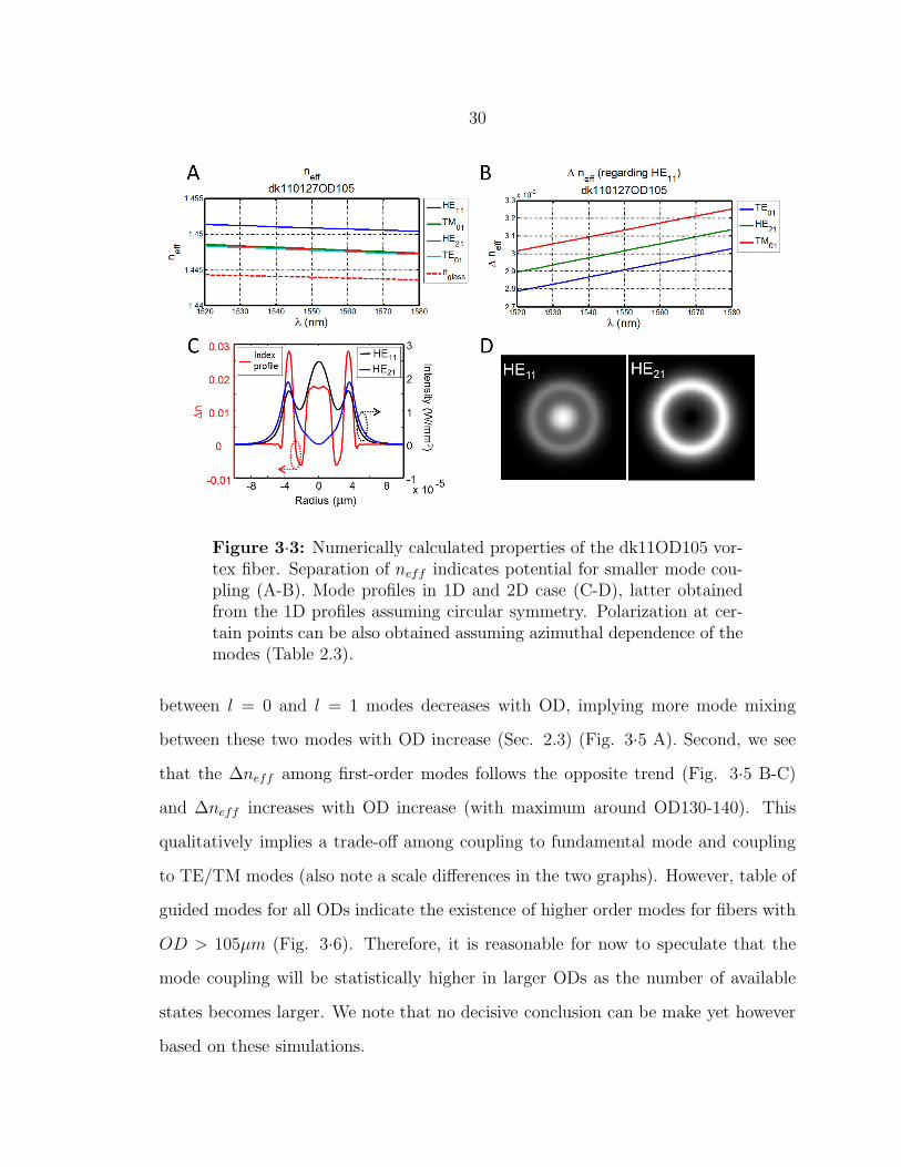
30

Figure 3·3: Numerically calculated properties of the dk11OD105 vor-tex fiber. Separation of neff indicates potential for smaller mode cou-pling (A-B). Mode profiles in 1D and 2D case (C-D), latter obtainedfrom the 1D profiles assuming circular symmetry. Polarization at cer-tain points can be also obtained assuming azimuthal dependence of themodes (Table 2.3).

between l = 0 and l = 1 modes decreases with OD, implying more mode mixing

between these two modes with OD increase (Sec. 2.3) (Fig. 3·5 A). Second, we see

that the ∆neff among first-order modes follows the opposite trend (Fig. 3·5 B-C)

and ∆neff increases with OD increase (with maximum around OD130-140). This

qualitatively implies a trade-off among coupling to fundamental mode and coupling

to TE/TM modes (also note a scale differences in the two graphs). However, table of

guided modes for all ODs indicate the existence of higher order modes for fibers with

OD > 105µm (Fig. 3·6). Therefore, it is reasonable for now to speculate that the

mode coupling will be statistically higher in larger ODs as the number of available

states becomes larger. We note that no decisive conclusion can be make yet however

based on these simulations.

31

Figure 3·4: (A) Effective indices for guided modes for the dk11OD160vortex fiber. (B) Corresponding LP notation designating certaingroups of modes.

Before we move onto the experimental part, we briefly want to note few physical

quantities that can be derived using the calculated effective indices, namely group

index (ng), group velocity dispersion (GVD) and effective area (Aeff) (Agrawal, 2010):

ngdef

= neff − λdneff

dλ, (3.1)

GV Ddef

= −λ

c

d2neff

dλ2, (3.2)

Aeffdef

=

(∫| E |2 dA

)2∫| E |4 dA =

(∫IdA

)2∫I2dA

, (3.3)

where c is the speed of light in vacuum, λ is wavelength, E is 2D electrical field

profile and the integral in Eq. 3.3 is over the fiber cross-section area. The wavelength

dependance of the three quantities for dk11OD105 is given in Fig. 3·7. We note that

GVD and Aeff of the HE11 mode in vortex fiber are similar to the properties of its

SMF counterpart (typical SMFs used for optical communications have Aeff of the

order of 100 µm2, some large mode area fibers above 1000 µm2 and some photonic

crystal fibers below 10 µm2).

32

Figure 3·5: Effective index difference (also called mode separation)versus fiber OD between different modes.

Figure 3·6: Table of guided modes for different OD fibers, at 1550nm.OD105 offers largest diameter fiber for which l ≥ 2 modes are cuts off.

3.3 Experimental measurements

In this section we experimentally measure some of the vortex fiber properties that we

numerically calculated in the previous section. Our experimental setup and methods

will be explained in detail in Ch. 4, and here we focus only on results.

33

Figure 3·7: Numerically calculated properties of the dk11OD105 vor-tex fiber

Figure 3·8: Measured and numerically calculated ∆neff with respectto the HE11 mode for (A) OD100, (B) OD110 and (C) OD115 vortexfibers.

3.3.1 Effective and group indices

The results of the measured effective indices for the three different ODs are shown

in Fig. 3·8, and are in relative good agreement with numerical results (juxtaposed

on the graph). We do note some difference between two results (on the order of

10− 20%) especially as we go to the higher ODs (Fig. 3·8 A-C). To understand this,

we’ll need the knowledge of mode conversion methods that we use (4.1). Namely,

our mode conversion method requires that stress is applied onto the vortex fiber, on

the order of 1kg. We believe that this stress, which increases with ODs as measured,

induces geometrical changes in the fiber that break down the cylindrical symmetry

34

assumption under which numerical results have been obtained (Smith, 1980; Golowich

and Ramachandran, 2005).

In addition to ∆neff , group index difference (∆ng) has also shown a good agree-

ment between the numerically calculated and measured values (Fig. 3·9) (see Sec.

4.1 for measurement details).

Figure 3·9: Group index difference among HE11 and HE21 vortexfiber modes for several different OD.

3.3.2 Loss

Power loss in fibers can be caused by material absorption, linear and nonlinear scat-

tering, macrobend and microbend losses (Smink et al., 2007). The measurement

procedure compared transmission power readings for different fiber lengths. Small

insertion loss (<0.1dB) can typically occur at the splices, especially for large ODs,

due to modal mismatch. In the case of dk11OD105 we measured loss of 1.3 ± 0.1

db/km for HE11 mode, and 1.6± 0.1 dB/km for HE21 (similar losses were observed

for different fiber ODs). The estimated 0.1dB/km error in the measurements comes

from power oscillations caused by distributed mode coupling (using bubble wrap to

thermally isolate helps stability timewise). Loss between HE11 and HE21 modes (also

called modal differential loss or excess loss (Olshansky and Nolan, 1976)) was mea-

sured to be 0.33±0.1 dB/km (Fig. 3·10. This effect is predicted theoretically and can

35

be explained by mode coupling theory where perturbations have longitudinal spatial

frequencies below the range required for mode coupling (Olshansky and Nolan, 1976).

We leave the detailed study of this effect for the future work.

Figure 3·10: Transmission power difference (in dB) between HE21 andHE11 modes showing linear dependence of the loss in length. Gradientof the fit 0.33 dB/km gives the excess (i.e. differential) loss betweenthe two modes.

3.3.3 Mode imaging

So far we have presented properties of the vortex fiber that show, numerically and

experimentally, the effective index separation of the modes. These results suggest

that OAM modes can exist in a vortex fiber. In order to verify that this is indeed

the case, we designed a setup for imaging both the intensity and the phase of the

output of the vortex fiber (Bozinovic et al., 2011b) (Fig. 3·11). A typical intensity

image is shown in Fig. 3·12 A, along with the OAM mode intensity profile along

the ring (Fig. 3·12 B). We note some intensity variations, that indicate interference

between multiple modes 3·12A. In Ch. 5 we explain a method that quantifies these

variations to find the relative mode contributions. In order to observe the phase of

the beam, a reference beam was introduced 3·11, and interference was observed in

the case of: slightly diverging fundamental (LG01 ∼ eiρ2

) mode (Fig. 3·12 C) and

36

Figure 3·11: Setup for OAM mode imaging. This setup enables us tomeasure both the intensity and the phase of the beam.

a tilted plane wave E = eikxx (Fig. 3·12 D). As we showed previously (Ch. 2), the

OAM modes have distinct exp(ilφ) phase. Using simple calcualtions for these two

interference cases, the intensity distribution in the image plane can then be written

simply as:

I1(ρ, φ) ∼ |eilφ + eiρ2 |2 = 2 + 2cos(lφ+ ρ2), (3.4)

I2(ρ, φ) ∼ |eilφ + eikxx|2 = 2 + 2cos(lφ+ kxx). (3.5)

The two patterns are plotted in Fig. 3·12 E-F are called spiral and fork patterns

respectively (and have been ubiquitous in OAM related literature (Andrews, 2008)).

The features of the simulated and measured patterns match well, confirming the

existence of the OAM modes at the fiber output (Fig. 3·12).

Finally, we compare the observed and numerically calculated mode profiles and

observe good agreement (Fig. 3·13 shows the case of OD100). This observation

indicates that numerical model that we used is to the great extent good approximation

of the measured values, and allows easy scaling to other OD values.

With this we proceed in the next chapter with the detailed explanation of the

mode conversion methods that we used in Fig. 3·11, as well as with the explanation

37

Figure 3·12: (A) OAM mode intensity profile and (B) a line pro-file along the ring. (C,D) Observed interference patterns betweenthe OAM mode and the reference beam when the two beams are (C)collinear or (D) form an angle . (E,F) Simulated interference patternsin the two cases.

of the effective and group index measurements (Fig. 3·8 and 3·9). Later in Ch. 5 we

develop methods for quantifying the modal purity that will give us better insight into

the vortex fiber properties.

38

Figure 3·13: Comparison of the simulated and imaged mode profilesfor OD100 case.

39

Chapter 4

OAM Generation in Vortex Fiber

Most of the conventional light sources, coherent or incoherent, emit light in a funda-

mental mode (LG00) and conversion to HOM is needed in order to create an OAM

beam. Methods that use phase plates (Khonina et al., 1992), cylindrical lenses (Pad-

gett et al., 1996), computer generated holograms (He et al., 1995), fiber gratings (Mc-

Gloin et al., 1998), q-plates (Karimi et al., 2012), specialty phase plates (Berkhout

et al., 2010) and photonic integrated structures (Cai et al., 2012) have been proposed.

In this chapter, we study two of these methods for OAM generation, based on:

• fiber gratings, specifically:

– microbend gratings (Hill et al., 1978),

– carbon-dioxide (CO2) laser induced gratings (Poole and Presby, 1995), and

• computer generated holograms, using liquid-crystal-on-silicon (LCoS) spatial-

light-modulators (SLM) (Ebihara et al., 1992).

While fiber grating methods have the advantage of mode conversion inside the fiber,

allowing easier device packaging and flexibility, hologram-based free-space coupling

methods have the advantage of allowing multiplexing, i.e. simultaneous coupling of

several beams.

40

4.1 Fiber Gratings

Following the success of diffraction gratings for distributed feedback lasers (Kogelnik

and Shank, 1972), first fiber gratings were introduced in 1978 (Hill et al., 1978). Fiber

gratings were used as mirrors, in which a forward-propagating mode guided by the

fiber core couples to a backward-propagating mode of the same type (Meltz et al.,

1989), and as mode converters, in which one type of guided core mode couples to

a different type (Hill et al., 1990; Poole et al., 1990). The fiber gratings were also

used as loss filters, by enabling the guided core mode to couple to radiation modes

(Mizrahi and Sipe, 1993) or for creating cladding modes, in the case where cladding

is surrounded by a medium with a refractive index lower than that of the glass, such

as air (Vengsarkar et al., 1996).

Applications of few-mode fiber gratings include dispersion control, signal power

management, switching and routing, polarization control and sensing (Ramachan-

dran, 2005). Based on the mode of operation, namely reflection or transmission

mode, fiber gratings can be classified into Bragg gratings and long-period gratings

(LPGs), respectively. In practice, LPG grating periods are usually on the order of

a millimeter (with typical lengths on the order of tens of millimeters), while Bragg

gratings have periods on the order of micron (Kashyap, 2008). Since we are interested

in mode conversion in transmission mode, here we focus on studying LPGs only.

Several methods to generate fiber gratings include photosensitive methods such

as UV-laser illumination in Ge-doped fibers (Meltz et al., 1989), microbend gratings

(Blake et al., 1986) and CO2 laser induced gratings (Poole and Presby, 1995; Davis

et al., 1998; Abrishamian et al., 2012)). Here, we focus on microbend and CO2

gratings as these produce anti-symmetric gratings (defined in the next section). The

biggest difference between these two methods is that microbend gratings are not

permanent and are easily tunable (on the order of seconds) in terms of their period

41

and length, while CO2 laser gratings are permanent and therefore non-tunable (mainly

offering much easier packaging and deployment).

4.1.1 Long period grating theory

The theory of fiber LPGs has been extensively studied (Hill et al., 1990; Poole et al.,

1990; Vengsarkar et al., 1996; Erdogan, 1997b; Erdogan, 1997a; Hwang et al., 1999;

Savin et al., 2000; Li et al., 2001) and relies on a coupled-mode theory (Marcuse,

1974), applied in cylindrically symmetric waveguides (such as fibers). In the general

case (also called asynchronous coupling), two co-propagating modes with the propa-

gation constants β will have the powers P1 and P2 after the grating of length Lg and

period Λ:

P2

P1= (κgLg)

2sinc2(√

κ2g + δ2Lg), (4.1)

where δ is a detuning parameter:

δ(λ) =1

2(β1 − β2)−

π

Λ, (4.2)

and κg defines the grating strength through a perturbation overlap integral:

κg =

∫~E1(~r)P (~r) ~E∗

2(~r)d~r, (4.3)

where P (~r) represents the perturbation and E(~r) electric fields of the two modes.

In the special case when δ = 0 (the so-called phase-matching condition), complete

(100%) mode conversion is theoretically achievable:

β2 − β1 =2π

Λ, (4.4)

Note that detuning parameter δ depends on the wavelength, hence grating mode

conversion described by Eq. 4.1 is also wavelength dependant (we’ll verify this ex-

42

perimentally in the next section).

In the case of the vortex fiber, we are interested in a perturbation that can couple

fundamental HE11 modes into OAM modes (comprising HEeven,odd21 modes as we saw

in Ch. 2). For this mode conversion, an antisymmetric grating i.e. the one for

which perturbation that has a functional form of P (~r) ∝ cos(φ), needs to be used (an

example of these gratings are microbend (Blake et al., 1986) and CO2 laser induced

gratings (Davis et al., 1998)). By looking at the functional form of the HEeven,odd21

modes (Tables 2.1-2.3), we note that they have cos(φ) and sin(φ) dependance. Using

following identities:

2π∫

0

cos2(φ)dφ = π

2π∫

0

cos(φ)sin(φ)dφ = 0,

2π∫

0

sin2(φ)dφ = π,

it can be shown that overlap integral Eq. 4.3 is non-zero only for pairs of modes:

(HEx11, HEeven

21 ) and (HEy11, HEodd

21 ). This reveals that for the phase matching con-

dition δ = 0 and κgLg = π/2, the HEx11 mode will convert into HEeven

21 and HEy11

into HEodd21 . Hence, a circular polarization at the grating input (HEx

11 + iHEy11) will

convert into OAM mode at the grating output (OAM+11 = HEeven

21 + iHEodd21 ), and

that can be achieved using a simple polarization controller. We note that Eq. 4.1

describes power immediately after the grating, and considers only the ideal case. As

we mentioned in Sec. 2.3, real fiber twists and bends can cause perturbations that

couple one OAM state to the other OAM state of opposite helicity.

4.1.2 Microbend gratings

As we mentioned, in the case of the microbend grating, the perturbation is created

by geometrical changes of the fiber. A convenient realization of microbend LPGs uses

a metallic block with grooves, that is pressed against the fiber (pressure lies in the

range of equivalent to a mass of 500g to 3kg (Savin et al., 2000). In our case, several

43

specially designed metallic blocks with various groove periods Λ0 (ranging 300µm

to 1000µm) were built, with a stress measuring gauge. In order to achieve different

grating periods it is then sufficient to rotate the block with respect to the fiber, in

which case the grooves form a certain angle, θ, with the straight-held fiber, and the

period becomes Λ = Λ0/cos(θ).

Figure 4·1: Microbend gratings. (A) Mode conversion setup. (B)Picture of the microbend grating. (C) Effective indices of modes sup-ported by the vortex fiber (also see 3·8). Microbend grating period canbe tuned to allow for mode conversion from HE11 to first-order modes(denoted by arrows).

A transmission setup that can monitor mode conversion across a wide range of

wavelengths was built (Fig. 4·1 A). In the setup, the light from the broadband

source (tungsten-halogen lamp) is guided through a single mode fiber (SMF) into the

vortex fiber onto which grating was applied. The vortex fiber is then spliced onto

44

a second SMF whose output is connected to an optical spectrum analyzer (OSA).

If the phase matching condition is satisfied at the grating, any higher order mode

that is created in the vortex fiber will not be guided into the second SMF, and a dip

in intensity transmission will occur in the OSA spectrum (also called resonance, or

loss transmission spectrum). A typical spectrum acquired in the case of vortex fiber

is shown in Fig. 4·1 D. Knowing that the vortex fiber splits the effective indices of

the first-order modes (Fig. 4·1 C), we observe three resonant dips that satisfy phase

matching conditions for the TM , HE21 and TE modes. The maximum conversion is

achieved when Λ = λ∆neff

for desired modes, where ∆neff corresponds to difference

between HE11 and TM01, HE21 and TE01 modes. This measurement was the basis

for the ∆neff measurement presented in Fig. 3·8. Note that the bandwidth of the

incoherent broad band source that we use is so large (> 500nm) that the light at the

grating input is unpolarized (for the same reason the light from incandescent sources

is unpolarized) . This means that one polarization, which contributes to the half of the

beam, converts to the TM01 and TE01 modes, while the other half stays unconverted.

This reasoning explains why the TM01 and TE01 resonances appear only 3dB strong.

In the case of the HE21 resonance, both polarizations will undergo conversion into

the degenerate HEeven,odd21 , and these mode conversion resonances overlap to create

stronger mode conversion (≈ −15dB or 97%).

In order to further study the properties of microbend gratings, we focus further

on the HEeven,odd21 resonances using a 1550nm LED source (bandwidth of ≈ 40nm,

enabling a higher degree of polarization). In addition, a polarization controller was

installed onto the SMF (Fig. 4·2 A). We observed that microbend gratings are highly

polarization sensitive devices (Fig. 4·2 B), with conversion oscillating from weak

−9dB(= 87.4%) under-coupling, to strong −25dB (or 99.7%) conversion. The reason

behind this lies in the fact that any stress on fiber inherently introduces asymme-

45

Figure 4·2: Microbend resonance characteristic with respect to inputpolarization, grating length and fiber roll angle. (A) Polarization de-pendence. (B) HE21 resonances for different grating lengths. Longergrating length require less pressure per fiber length, hence, pressure in-duced splitting is smaller. Note grating bandwidth change with length,in agreement with the theory. (C) Microbend pressure for HEodd

21 andHEeven

21 resonances vs fiber roll angle (i.e. rotation axis is along thefiber).

try in the otherwise circularly symmetric fiber. This asymmetry (that manifests in

non-zero elipticity) introduces birefringence for the two polarization modes, resulting

in a shifted resonance. In addition to induced birefringence (observed through reso-

nance shift), we note a change in the grating strength (κg in Eq. 4.3) for different

polarizations, leading to conclusion that κgLg 6= π/2 for all the polarizations. We

further observe the role of the grating length (Fig. 4·2 C). As the length of the grat-

ings changes, the grating pressure per length changes in a sense that shorter gratings

(Lg = 20 mm), exhibit more pressure per length then 100mm long grating. There-

fore, shorter grating induce more birefringence and larger separation among the two

46

HEeven,odd21 mode resonances.

At the end of the microbend grating study, we study the effect of the fiber roll

angle (rotation around the fiber axes). We note that for certain fiber orientation

(in this case at 100o angle) the same pressure can be used for both HEeven,odd21 res-

onance so κxg = κy

g , however the induced birefringence (i.e. resonance splitting) is

still unavoidable. Nevertheless, this points to the important fact that vortex fiber is

essentially not perfectly cylindrically symmetric but instead exhibits some degree of

ovality. Measuring the degree of ovality is left for future work.

4.1.3 CO2 laser induced gratings

CO2 laser-induced gratings are compact device that offer reduced sensitivity to the

environment and convenience for deployment (Poole and Presby, 1995). It has been

shown that CO2 laser gratings change both the geometry of a fiber as well as the re-

fractive index of the core and cladding in such a way as to achieve anti-symmetric per-

turbation (Abrishamian et al., 2012). CO2 lasers operate at a 10.2µm wavelength and

typically have high powers (in our case ≈ 10W ), which can easily create permanent

glass deformations. In order to test the feasibility of CO2 gratings for future device

deployment, a setup capable of point-by-point LPG writing was built (Fig. 4·3 A).

The laser beam was first expanded to the size of D ≈ 20mm, and then focused onto

the vortex fiber using f = 60mm lens, producing spot size of Φspot =4λfπD

≈ 40µm. Us-

ing a powermeter that was placed behind the fiber, one was able to measure whether

the beam would hit the fiber, in which case most of the power would be absorbed by

the glass and a small portion of the beam would be transmitted. After several setup

iterations, a relatively repeatable procedure was developed for grating manufacturing

(see next section for detailed step-by step instructions). The microscope image of the

fiber, after the grating has been inscribed, clearly indicates periodic changes (Fig.

4·3 C). Unlike in the microbend case, the CO2 grating exhibited smaller polarization

47

sensitivity (Fig. 4·3 D), however, the current technique allowed for > 10dB(= 90%)

mode conversion. The ripples in the resonances are typical for multi-path interference

(MPI) and are an indicator of incomplete mode conversion. We discuss this effect in

more details in Sec. 4.1.4.

Figure 4·3: CO2 laser induced gratings. (A) Setup. Laser beam isfocused onto the fiber and point-to-point grating is written onto thevortex fiber. (B) Setup photo (blue line indicates beam path, red lineindicates vortex fiber). (C) Microscope image of the grating inscribedin the fiber, indicating periodic mechanical changes. (D) Polarizationdependence of the CO2 gratings. In comparison to microbend gratings(Fig. 4·2), CO2 gratings are less polarization sensitive.

CO2 laser grating writing procedure

Described below is the detailed procedure for point-by-point CO2 laser grating writ-

ing for a setup in the NFNO lab (concluding by January 5th 2012). The goal of this

procedure is to describe the current technique (admittedly there is a room for im-

48

provement). Before describing the procedure, we note few causes for common fiber

breaks and grating failures: 1) bad fiber clamping can cause fiber to snap or allow

tension to change during writing process, 2) fiber from which the coating is stripped

down can be scratched when in contact with the hard surface (beakers, optical table,

etc.), causing the fiber to break, 3) placing heavy objects (fiber spool for example) on

a fiber at any time should be avoided, 4) sudden yanks of the fiber during handling

can likely break the fiber, so slow fiber movements are suggested. The procedure for

grating writing goes as follows.

• Turn on a water pump and check if the water flow is 2 - 2.5 GPM. Set the

acid heater to 300oC. Turn on the CO2 laser controlled by a function generator

(Agilent E4420B), with the the following LF out settings: LF Out Amplitude:

5.0 Vp, LF Out Source: Func Generator, LF Out Waveform: Pulse, LF Out

Period: 200.0 sec (do not change this value), LF out Width: 8.0-200.0 s (this

number can be used to adjusted CO2 power, and is calibrated in the control

software below; 20-30 s might already be very powerful for writing!). Turn on

HeNe laser (provide 5V from DC power supplier HP E3632A), OSA, electronic

polcon and computer. Software used for writing is located here:

\eng_research_fibers\_programs\CO2 grating Labview software Nenad

• Measure the beam spot size of a laser one time only using a translating blade

procedure. The spot size should be almost diffraction limited, i.e. 1.22λ/NA

for 1/e2-diameter waist.

• Strip off small amount (≈ 50mm) amount of coating in the Sulfuric acid

(93%H2SO4and 7%N2H3; common proportion is 200ml:15ml). Be careful not

to touch beakers or any other hard surfaces as they can create a microscopic

crack in the fiber glass. Dip the fiber into IPA and then methanol to wash off

the excess acid. Use pen marker to mark the stripped fiber area. Clamp the

fiber into a translation stage. Be aware of the stage limit points.

49

• Set the tension of the fiber to approx. 200 grams. Use LF on/off on the function

generator to turn CO2 laser on/off. Focus the laser onto fiber with low power

(≈ 0.1W ), and place the power meter behind the fiber. Minimize the power by

moving the lens in the longitudinal (z) direction, so the fiber absorbs most of

the laser power, indicating that the fiber is close to the beam waist. Keep the

aperture before the focusing lens closed as lower NA is easier to work with. Only

the aperture after the beam expander should be used, the one after the mirror

should stay open. Minimize the power by moving the mirror in the vertical

direction only. Write down the name of the grating starting by date, increase

power (≈ 5.5W ). Make sure you have enough space for translation (≈ 50mm).

Acquire reference with the OSA. Enter the grating period in the software. Start

writing the grating.

• As the resonance is growing, tune the polcon to maximize it. At some point

the deepest resonance will stop growing and start over-coupling. Observe the

second resonance that sits on the other side of the Poincare sphere. These two

polarizations have different coupling strengths (a.k.a. κg). As κg1L is dropping

the κg2L will be increasing. The goal is to stop writing when κg1L = κg2L. It

is possible to follow resonances one grating line at a time in real time. Stop

writing the grating. Skillfully remove the fiber and put it in the foam holders.

Acquire spectra.

• Shut down the lasers (function generator for CO2 and DC power supplier for

He-Ne, turn off the interlock, power supplier, and He-Ne button in the black

homemade controller box, unplug laser power cable). After 10 minutes turn off

the water pump chiller (check distilled water status). Turn off the acid heater.

• Depending on the phase matching conditions of the fiber, CO2 gratings have

50

showed that the grating resonance can be shifted by approximately a few nano-

meters if heated. This shift is not permanent.

4.1.4 Role of tapers in improving mode conversion

In a general sense, a fiber taper is a in-fiber device on the order of tens of millimeters

in size, created in a multimode or few-mode fiber, that in our case enables small fiber

segment to become single-moded (Birks and Li, 1992). In this section we discuss how

this fact can improve the OAM mode quality and we experimentally verify improved

mode conversion.

So far, all the resonance measurements (Fig. 4·2 B, 4·3 D) required a splice be-

tween i) a SMF and ii) a vortex fiber that supports few modes (Fig. 4·2 A). However,

in the case of an imperfect splice (offset and angle splice), the fundamental mode

originating from the SMF can have a non-zero overlap integral with the vortex fiber

HOM, therefore making the splice itself act as a mode converter. This property,

however, negates the mode conversion created by the subsequent fiber grating since

gratings are reciprocal devices. If all of the HE11 mode converts to HE21, by reci-

procity, an imperfect splice will create several modes to co-exist in fiber. Since these

modes have different propagation constants, mode beating (or MPI) will occur, which

can be observed as ripples in a resonance (Fig. 4·3 D).

A relatively easy solution for this problem lies in tapers, that can can be used to

make near-perfect devices that do not allow mode coupling. Essentially, taper on a

multimode fiber acts as a mode stripper, coupling all the unwanted HOM modes (that

could have been created in the imperfect splice) into radiation modes that disappear

from the fiber after short propagation length. An important observation is that the

taper needs to exist in a medium that has a refractive index larger or equal to that of

the cladding refractive index (for this purpose index-matching gel or oil is used). If

this step is omitted, rather then to radiative modes, fundamental mode will convert

51

into cladding modes that can still have a detrimental effect on mode purity.

Figure 4·4: (A) Tension and fiber width profile for a 5-5-5µm tapergeometry with 40µm waist. (B) Resonance for dk11OD100 fiber in thecase of a taper shown in A.

Tapers in vortex fibers were formed by stretching the fiber in a heat source using

a tapering station (Ring of Fire, 3SAE Technologies). The shape of the taper for this

case has been previously studied (Birks and Li, 1992). We used 5-5-5mm geometry

(where 5mm refers to the length of each of the three taper regions: downtaper region,

waist and uptaper region) and a 40µm waist size (Fig. 4·4 A). The three tuning

parameters were arc powers for the 1) downtaper region, 2) waist and 3) uptaper

region. The basic principle was to develop a procedure that will keep a very low

tension, though always larger then zero so the fiber is kept straight, with the starting

point at about 10 grams. The tension typically drops when the tapering process

starts and goes up at the end of the process (typical tension profile is plotted in Fig.

4·4 A). The heat arcs should be adjusted so the tension stays as low as possible,

optimally less then 10g (tensions of >30g did not perform well). Using the developed

tapering procedure, mode conversion of 35dB = 99.97% can be achieved (Fig. 4·4)

with fairly good repeatability of several devices in a row. The power numbers did

however vary for different fiber ODs, and at this level, only an empirical procedure

52

has been developed. The taper procedure is unidirectional in nature, meaning the

heat arc will sweep the fiber only in one direction as the fiber is being pulled.

4.1.5 Group index difference calculation

In this short segment we describe two methods to calculate group index difference

between theHE11 mode and a desired mode (Ramachandran, 2005). The first method

is based on a resonance parameter fitting. As we previously mentioned, the resonance

can be described as a sinc function Eq. 4.1, where we again rewrite equation for

detuning parameter δ:

δ(λ) =1

2(β1(λ)− β2(λ))−

π

Λ. (4.5)

If we now Taylor expand this equation around the resonant wavelength λres, and use

the fact that detuning parameter becomes zero for λres (i.e. ∆neff = λres/Λ) we can

write:

δ(∆λ) = −π∆λ∆ng(λres)

λ2res

= D0∆λ, (4.6)

where ∆ng is a group index difference (that we are looking to determine), and we

define D0def= −π∆ng(λres)

λ2res

, which represents the slope of δ(λ) curve.

In practice, in order to calculate the group index difference (∆ng), the resonance

is fitted using Eq. 4.1 (see Fig. 4·5) which would then provide the slope of the

detuning parameter function D0 = δ′

(λ). Knowing this, simple operations lead to

estimating ∆ng,HE11−HE21@1550nm = −λ2

resD0

π= −(2.7 ± 0.1) × 10−3, in the case of

dk110127OD100 fiber.

The second method to measure the group index difference is by observing several

resonant wavelengths for different microbend gratings (Fig. 4·6). Grating period Λ,

resonant wavelength and effective index difference ∆neff are related by ∆neff (λ) =

53

Figure 4·5: Loss transmission spectrum for HE11 and HE21 phasematched case. Fitting the curve with the expected sinc2 profile givesthe group index difference ∆ng.

λ/Λ(λ). Taking the derivative of this equation with respect to wavelength, one finds:

∆ng(λ) = ∆n2eff (λ)

dΛ

dλ=

(λ

Λ(λ)

)2dΛ

dλ. (4.7)

Using this method for the example of the dk110127OD100 fiber, we experimentally

obtained a ∆ng value between the HE11 and HE21 modes at 1550nm to be ∆ng =

−2.8×10−3, which is in agreement with the value obtained previously. Plots of ∆neff

and ∆ng at different wavelengths are shown in Fig. 4·6.

4.2 Spatial light modulator approach

The LCoS SLM is a device that can very precisely control a phase front of beam (He

et al., 1995). Application of SLMs include optical beam pattern forming (Matsumoto

et al., 2008) and aberration correction (Friberg and Dandliker, 2008) (Fig. 4·7). In

our case, an SLM is used to create a free-space OAM mode which is then coupled

into a cleaved vortex fiber. This method, unlike fiber gratings, allows for multiplexing

54

Figure 4·6: Phase matching curves Λ(λ) relate grating periodΛ with resonant wavelength (particular example is for the case ofdk110127OD100 fiber). Respective ∆neff and ∆ng can be calculated(bottom two graphs).

several beams at the same time.

A setup built for OAM mode generation in a fiber is shown in Fig. 4·8. SMF

output is collimated and reflected off the LCoS SLM (Hamamatsu, X10468-8). Here,

we use an on-axis conversion using a beam-splitter (in later chapters an off-axis con-

version is used to avoid 3dB loss from the beam-splitter). Care must be taken to make

the SLM, and all the other optical components, stable. Also, the SLM can modulate

only one polarization that is aligned with the orientation of the liquid crystals. Two

mirrors and pinholes were used to align the beam onto the SLM with the spiral pat-

tern applied. After reflection from the SLM, a donut beam carrying orbital angular

momentum is observed on the camera and the spiral pattern is adjusted in order to

obtain a donut shaped mode with the least variations (Fig. 4·9).

In order to couple the beam into the fiber, a telescope made of two f = 200mm

lenses relayed the beam onto the objective (for larger beams this step is not necessary

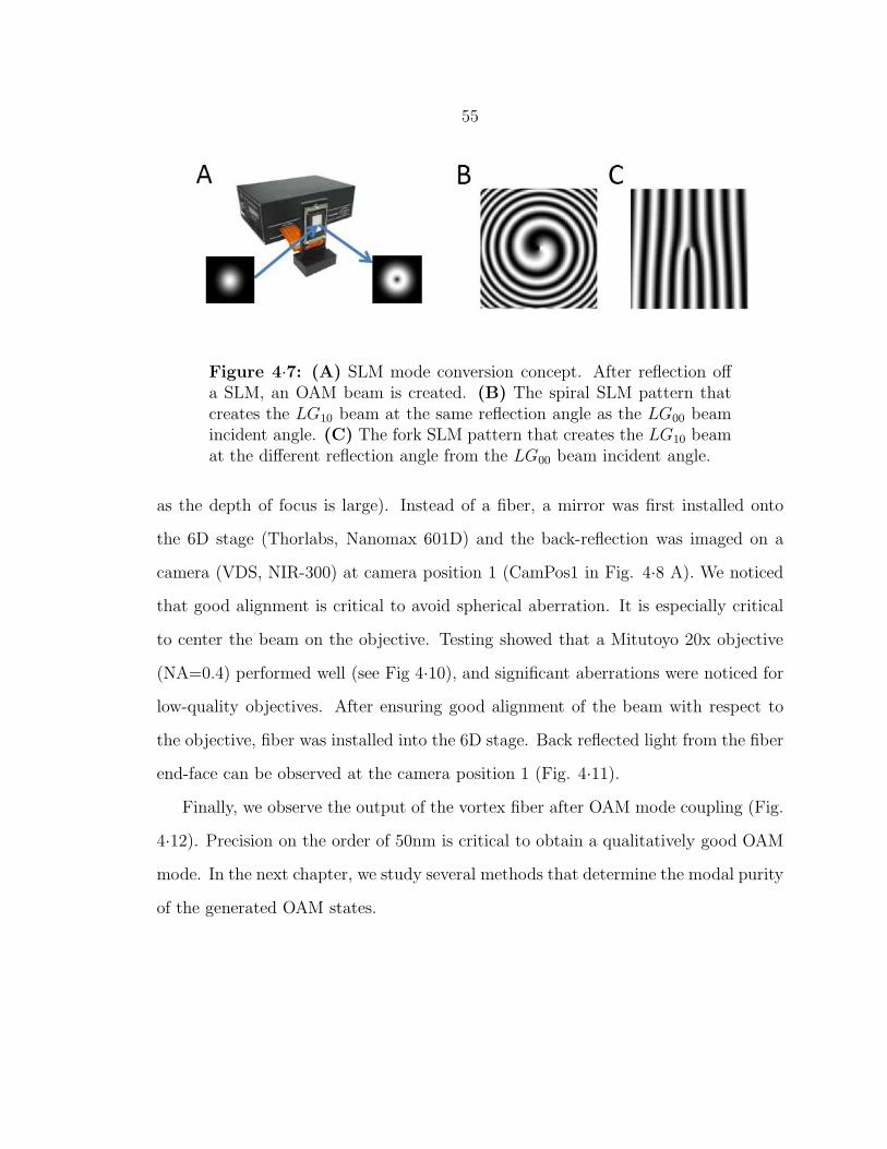
55

Figure 4·7: (A) SLM mode conversion concept. After reflection offa SLM, an OAM beam is created. (B) The spiral SLM pattern thatcreates the LG10 beam at the same reflection angle as the LG00 beamincident angle. (C) The fork SLM pattern that creates the LG10 beamat the different reflection angle from the LG00 beam incident angle.

as the depth of focus is large). Instead of a fiber, a mirror was first installed onto

the 6D stage (Thorlabs, Nanomax 601D) and the back-reflection was imaged on a

camera (VDS, NIR-300) at camera position 1 (CamPos1 in Fig. 4·8 A). We noticed

that good alignment is critical to avoid spherical aberration. It is especially critical

to center the beam on the objective. Testing showed that a Mitutoyo 20x objective

(NA=0.4) performed well (see Fig 4·10), and significant aberrations were noticed for

low-quality objectives. After ensuring good alignment of the beam with respect to

the objective, fiber was installed into the 6D stage. Back reflected light from the fiber

end-face can be observed at the camera position 1 (Fig. 4·11).

Finally, we observe the output of the vortex fiber after OAM mode coupling (Fig.

4·12). Precision on the order of 50nm is critical to obtain a qualitatively good OAM

mode. In the next chapter, we study several methods that determine the modal purity

of the generated OAM states.

56

Figure 4·8: Spatial light modulator based mode conversion. (A)Setup. (B) Photo of the setup.

Figure 4·9: Spiral and fork holograms that create LG∗10, showing the

effect of tilt in the case of the fork hologram.

57

Figure 4·10: Back-reflection from the mirror installed instead of thefiber for three different axial positions of the coupling stage for a beamfree of aberrations: (A,C) defocused LG00 (B) focused LG00 (D,F)defocused LG10 (OAM mode)(E) focused LG10. Symmetric pattern,indicates good alignment between input beam and the fiber.

Figure 4·11: Camera image at the CamPos1 for the vortex fiber in-stalled. Donut mode represents back reflection from the fiber end-face(similar to the case of the mirror in the Fig. 4·10). HE11 mode rep-resents light coming out of the vortex fiber, when the other fiber endis connected to the light source. Two images here are intentionallymisaligned.

58

Figure 4·12: Output of the vortex fiber after OAM mode coupling.(A) Aligned and (B) misaligned case.

59

Chapter 5

OAM Purity Measurements

In previous chapter, we studied two methods for OAM mode generation in fibers and

showed results that qualitatively confirm the existence of OAM states. In this chapter

we quantitatively study OAM mode purity using two methods:

• Ring method (Bozinovic et al., 2012a), and

• Regression analysis (Golowich et al., 2013)

These techniques allow us to obtain measure of OAM mode power for different fiber

lengths allowing us to track their evolution in vortex fibers.

5.1 Ring technique

In Sec. 4.1.2 we demonstrated how microbend gratings create OAM state, and ob-

served the helical phase of these modes using interference with the expanded Gaussian

reference beam. The ring technique that we introduce here is a method to quantify

OAM mode purity using image analysis. In particular, the ring technique requires

acquisition of the two circular polarization projections, acquired simultaneously.

An imaging setup built for this purpose is shown on Fig. 5·1, and it can be

considered an extension of Fig. 4·1. A 3dB coupler is used to combine two sources:

1) a 50nm-wide 1550nm LED, and 2) a 100kHz narrowband CW tunable external

cavity laser (ECL) (Agilent 8168F). One arm of the 3dB coupler is spliced to a vortex

fiber using standard splicing equipment (Ericsson FSU 995). A microbend grating

60

(40mm length, 475µ m period), with only the LED source turned on, converts the

fundamental mode of a SMF into the desired HEodd21 mode with 18dB conversion

efficiency (Fig. 5·1 B). After the desired mode coupling is obtained for a desired

wavelength (in this case, 1527 nm), the source is switched from LED to the ECL

laser. The vortex fiber is then cleaved after the output of the microbend and placed

at the fiber stage for imaging.

Figure 5·1: Setup for imaging vortex fiber output. (A) Experimen-tal setup that uses grating for OAM mode generation. (B) Gratingresonance spectrum used to deduce HEo

21 mode conversion level. (C)Camera image of the four polarization projections of the fiber output.Acronyms: left circular (LC), right circular (RC), vertical (V) and hor-izontal (H), non-polarizing beam splitter (NPBS), quarter wave plate(QWP), polarizing beam displacing prism (PBDP). Vertical (V) po-larization projection was interfered with the reference beam (Ref.) inorder to observe the phase of the vortex beam. Showed is the l = +1OAM state that is circularly polarized (spin = 1).

In order to obtain two desired polarization projections (LC and RC) as well as

61

ability to image a phase of a beam simultaneously, a combination of non-polarizing

beam splitters (NPBS), quarter wave plates (QWP) and polarizing beam displacing

prisms (PBDP), is used. In particular, left circular (LC), right circular (RC), vertical

(V) and horizontal (H) projections were obtained. An example of an image acquired

at the camera (VDS, NIR-300, InGaAs, FOV: 10mm X 8mm) is shown in Fig. 5·1

(C), where the vertical (V) polarization projection was interfered with the reference

beam (Ref.) in order to observe the phase of the beam.

In a free-space, a linear combination of the l = ±1 OAM modes has been shown to

have a total OAM of topological charge that lies between −1 ≤ l ≤ 1 (Schmitz et al.,

2006). Similarly, one can ask how to achieve this linear combination in the case of a

fiber. The answer is very simple and draws analogy from the two polarization states

in the SMF, namely, a linear combination of the two OAM l = ±1 fiber modes with

arbitrary relative amplitudes can be obtained using commercial polarization controller

mounted on the vortex fiber (PolCon2 on Fig. 5·1). Verification of this can be seen

on Figure 5·2, where positions of the polcon2 paddles have been tuned to achieve

different OAM states, in particular, the state was tuned from l = 1 (Fig. 5·2 A) to

l = −1 (Fig. 5·2 C). The reason for this lies in the fact that bend-induced-stress of a

polarization controller can couple one OAM state into other, since two OAM states

are degenerate (similar effect is observed with two polarizations of a fundamental

mode, HEx,y11 ).

In the general case of the vortex fiber under study (dk110127OD100), light at

the vortex fiber output can contain contributions from the six vector modes: HEx,y11 ,

HEeven,odd21 , TM01 and TE01 (Snyder and Love, 1983). To analyze the purity of the

62

Figure 5·2: Camera images for the three positions of the polcon2paddles, tuned to achieve (A) l = 1, (B) l = 0 and (C) l = −1 state.

OAM states it is more convenient to introduce a so-called vortex basis set:

V+11(r, θ)

def= (HEx

11 + iHEy11) /

√2 = (x+ iy)F01/

√2

V−

11(r, θ)def= (HEx

11 − iHEy11) /

√2 = (x− iy)F01/

√2

V+21(r, θ)

def= (HEe

21 + iHEo21) /

√2 = eiθ(x+ iy)F11/

√2

V−

21(r, θ)def= (HEe

21 − iHEo21) /

√2 = e−iθ(x− iy)F11/

√2

V+T (r, θ)

def= (TM01 − iTE01) /

√2 = e−iθ(x+ iy)F11/

√2

V−

T (r, θ)def= (TM01 + iTE01) /

√2 = eiθ(x− iy)F11/

√2

where we have used the fact that, for this fiber, the vector modes may be accurately

expressed as linear combinations of LP modes through the weak guidance approxi-

mation, and Flm(r) denote the radial wave functions of the LPlm modes (Snyder and

Love, 1983). Note that in this representation, the V+,−21 modes correspond to the

desired OAM states in the fiber. The total electric field can be expressed as:

E(r, θ) =∑

l=[11,21,T ]

∑

s=[+,−]

γsl V

sl (r, θ), (5.1)

where γsl are the mode field complex amplitudes of the normalized vortex basis vectors.

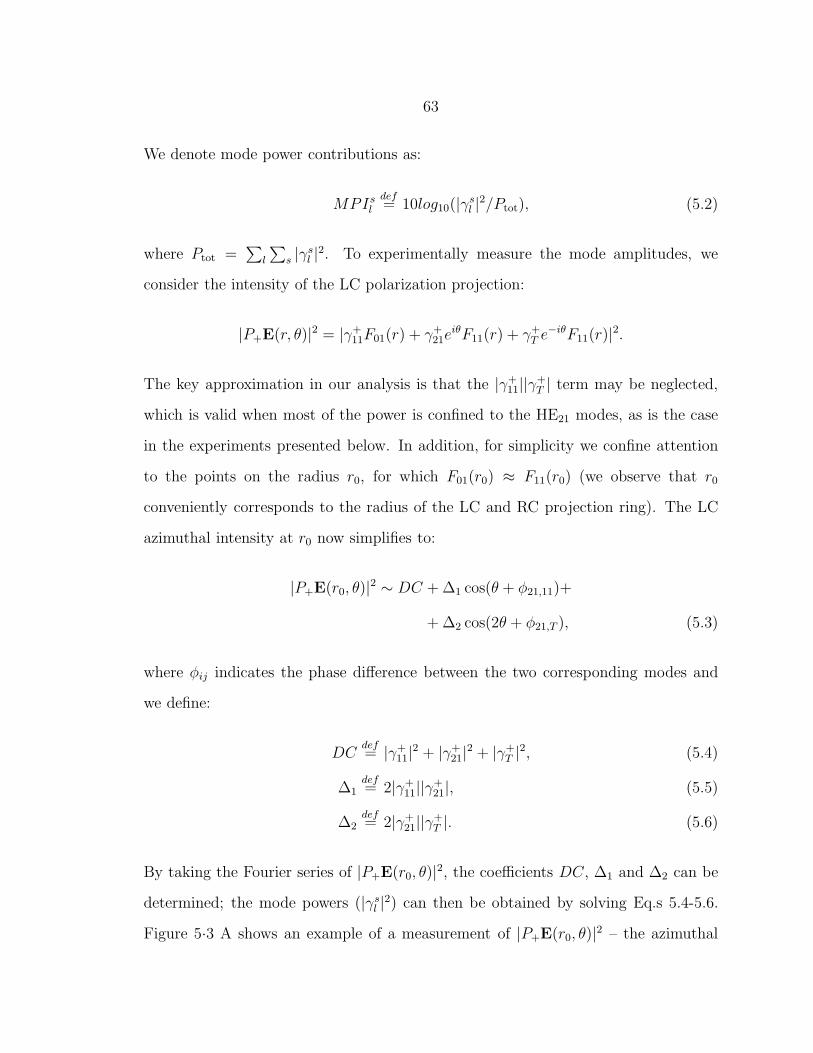
63

We denote mode power contributions as:

MPIsldef= 10log10(|γs

l |2/Ptot), (5.2)

where Ptot =∑

l

∑s |γs

l |2. To experimentally measure the mode amplitudes, we

consider the intensity of the LC polarization projection:

|P+E(r, θ)|2 = |γ+11F01(r) + γ+

21eiθF11(r) + γ+

T e−iθF11(r)|2.

The key approximation in our analysis is that the |γ+11||γ+

T | term may be neglected,

which is valid when most of the power is confined to the HE21 modes, as is the case

in the experiments presented below. In addition, for simplicity we confine attention

to the points on the radius r0, for which F01(r0) ≈ F11(r0) (we observe that r0

conveniently corresponds to the radius of the LC and RC projection ring). The LC

azimuthal intensity at r0 now simplifies to:

|P+E(r0, θ)|2 ∼ DC +∆1 cos(θ + φ21,11)+

+ ∆2 cos(2θ + φ21,T ), (5.3)

where φij indicates the phase difference between the two corresponding modes and

we define:

DCdef= |γ+

11|2 + |γ+21|2 + |γ+

T |2, (5.4)

∆1def= 2|γ+

11||γ+21|, (5.5)

∆2def= 2|γ+

21||γ+T |. (5.6)

By taking the Fourier series of |P+E(r0, θ)|2, the coefficients DC, ∆1 and ∆2 can be

determined; the mode powers (|γsl |2) can then be obtained by solving Eq.s 5.4-5.6.

Figure 5·3 A shows an example of a measurement of |P+E(r0, θ)|2 – the azimuthal

64

intensity variation of the image that occurs due to interference between the V+21, V

+11

and V+T modes. Figure 5·3 (B) shows the example of the Fourier series analysis, and

5·3 (C) illustrates the powers of the extracted modes. An equivalent procedure was

also repeated for the RC projection to calculate amplitudes of the negative helicity

modes.

Figure 5·3: Ring method analysis for determining modal content of thevortex fiber. (A)Azimuthal intensity profile of LC projection for radiusr0. (B) Fourier series coefficients for profile in (A). (C) Extractedmodal power contributions.

The high purity of the vortex states implies that only two modes – the HEeven,odd21

pair – are dominantly present in the fiber. Here, we would like to emphasize the

analogy of the two HE21 modes with the two linearly-polarized fundamental modes –

65

HEx,y11 . As with the two fundamental modes, we first note that since the HE21 modes

are degenerate, they can easily couple to each other under controlled perturbations.

Second, just as a linear combination of two fundamental modes with ±π/2 phase shift

will create a circularly polarized state, the same linear combination of the two HE21

modes results in an OAM state. This analogy has also been elegantly represented by a

higher order Poincare sphere by other authors studying OAM (Padgett and Courtial,

1999; Milione et al., 2011). A general linear combination of the two l = ±1 OAM

modes will have a topological charge with non-integer OAM (Schmitz et al., 2006).

In order to show the ability of the system to control OAM, camera images were

observed and analyzed while the polarization controller (PolCon2 on Fig 1a) was

manually tuned using adjustable paddles. Figure 5·4 (A) shows the modal power

distribution as the system was tuned through the different linear combinations of

the vortex states. In particular, Fig. 5·4 (B) shows observed camera images for the

pure V+21 state (A), linear combination of the vortex states (B) and the pure V−

21

state (C). Note that using a quarter wave plate, V+,−21 states can be converted to the

conventionally constructed linearly polarized OAM states. Our calculation showed

that the combined power of the undesired V+,−T and V+,−

11 modes mostly stayed below

a level of -15 dB (3%).

To estimate the error of the method described, a simulated data set has been

created with known contributions of each of the vortex basis vectors. Empirically

estimated dark noise was first added, followed by adding shot noise (st.dev=√N

where N is pixel count), finally subtracting the dark noise from the obtained image.

The data set was then analyzed and the original and the recovered mode powers were

compared. Estimated errors were <0.01 dB, ≈0.2 dB and ≈ 0.2dB for the V+,−21 , V+,−

T

and V+,−11 modes respectively. With this demonstration we conclude that our system

can create any linear combination of OAM states (−1 ≤ l ≤ +1), in a controllable

66

Figure 5·4: Ring method analysis applied in real time. (A) Modepowers in time during continuous adjustment of the paddles of PolCon2(on the vortex fiber) to obtain desired OAM state superposition. (B)Camera images of the three positions (a-c).

fashion.

Few comments on the experimental limitations of the Ring technique need to be

mentioned. In particular, we noticed that the beam-splitters we used had ≈ 3%

transmission difference for s and p polarization, and were slightly birefringent. Both

of these factors underestimate the measured vortex mode purity. Since the modal

content can be determined using only two polarization projections, we were able to

simplify the setup at the expense of not having the four projections. By doing this,

we observed a 6 dB lower power for the V+,−T modes, suggesting that the use of better

optical components can enable more accurate purity measurements. In addition to

the optical components, we noticed that the camera dark noise level introduces a limit

67

Figure 5·5: Ring method error estimation. (A) Random simulated

image created as an weighted average of the six modes V +,−21 V +,−

T andV +,−11 with randomized phases (dark and shot noise were also accounted

for). (B-D) Estimated modal power error with respect to differentinitial modal powers for (B) V +

21 , (C) V +T and (D) V +

11 modes. Wesee that errors on average increase as input powers of spurious modesincrease, indicating that the assumed ’dominant mode model’ is nolonger valid. For this reason calculations were only done for powers< −5dB with respect to total power.

for the V+,−21 vortex state sensitivity of 20 dB. Note that this limit does not apply to

the V+,−T and V+,−

11 modes, as their amplitudes are obtained from the interference

effects and not the DC power measurements. We expect that a camera with lower

dark-noise count will improve this sensitivity too.

In addition to the modal weights, relative phase information can also be extracted

by analyzing four independent polarization projections (Berry et al., 1977). However,

while we acquire four polarization projections simultaneously, only three of them are

independent (H + V = RC + LC). Therefore, in our case, only half of the Poincare

68

sphere can be covered (Fig. 5·6 B).

Figure 5·6: (A) Concept of higher-order Poincare sphere (taken withpermission from (Milione et al., 2011)). (B) Reconstruction of a rela-tive phase between two OAM states for the same case of tuning OAMshown in Fig. 5·4.

5.2 Cutback measurements

In this section, we analyze the relative mode powers for different fiber lengths using

the ring technique described previously (Sec. 5.1). We show that mode purity deteri-

orates with length, nevertheless still preserving good purity (Bozinovic et al., 2011b;

Bozinovic et al., 2011a). Since mode coupling is affected by the wavelength of light

as well as the fiber temperature (Marcuse, 1974), at a particular fiber length, relative

modal powers were determined for 500 different wavelengths within a 0.5nm range.

Figure 5·7 (A-C) shows the relative mode powers for the three dk11OD115 lengths

(360m, 720m, and 1020m) in the case od high purity, > 20dB, OAM+ mode excita-

tion at 1550 nm. Note how the OAM mode power deteriorates with length and the

relative mode powers of other modes increase. A stress-induced microbend grating

with L = 40mm length and Λ = 475µm grating-period was used for mode generation,

69

and prior to the grating, the fiber was securely taped to be free of any movements

that would change phase or polarization, and therefore, coupling conditions at the

grating input. The results were obtained by measuring modal power ratios for a

long fiber length first, which was then sequentially shortened (this procedure ensures

that the same input launch conditions existed for all lengths that were measured).

As we observed, different relative mode powers have been obtained for the different

wavelengths due to wavelength-induced phase changes, that in turn induced different

coupling conditions. We note that a larger bandwidth source would effectively per-

form averaging over wavelengths, but emphasize the only narrow linewidth source can

be used to ensure visibility of the modal interference, necessary for power calculations.

Figure 5·7 (D) shows results of relative mode powers for the several fiber lengths,

where each point denotes a mean relative mode power value with one standard devia-

tion from the mean. After 1.1km of propagation of the desired OAM modes, less than

−10dB of the input power leaked into the LP±

01 and the TM01 and TE01 modes. we

use a tunable continuous wave external cavity laser (CW-ECL, Agilent 8168F) with

100kHz linewidth (coherence length 3km) to capture necessary modal interference

effects between the modes after 1.1-km of propagation in the vortex fiber (the maxi-

mum optical-path length delay, given by ∆ngL = 3m, where ∆ng is the difference in

group index between modes, is ≈ 3 meters).

In addition to wavelength, the relative mode powers are also measured in time

(Fig. 5·7E), indicating temporal stability on the order of hours (though additional

correction adjustments were needed on a longer time scale).

70

Figure 5·7: (A-C) Relative mode powers for three different lengths forthe case of high purity (> 21dB) OAM+ mode excitation at 1550 nm(OAM power refers to combined OAM+ and OAM− mode powers, andLP01 refers to combined powers of the two LP±

01 states). (D) Measuredmodal power ratios as a function of fiber length for the same case asin A-C. (E) Relative mode powers with respect to time, showing thetemporal stability of the OAM modes.

5.3 Regression analysis

In addition to the Ring method that uses the dominant mode approximation, here

we describe a method that applies more rigorous mathematical analysis to obtain

relative mode powers without the dominant mode approximation (Golowich et al.,

2013). Here we describe the idea of the method and would like to refer a reader to

the mentioned paper for more details. In particular, method is based on regression

analysis of four polarization projections, and includes analysis of not only azimuthal

intensity distributions at one radius, but the total spatial intensity distribution of

the modes. In addition, the method also relies on pure mode intensities as prior

71

information. An additional advantage of the regression method is that it allows the

relative phases of the modes to be obtained (for example the relative phase difference

between HEeven,odd21 modes), in addition to the modal powers.

Figure 5·8 (A) shows calculated modal powers after L = 3m long propagation

in a dk11OD100 fiber. Power were estimated for each of the three pairs of modes

HE11, HE21, and TE01/TM01, for a range of wavelengths surrounding the microbend

grating resonance for the HE21 mode. The HE11 mode power vs wavelength was also

compared with the one obtained using OSA loss-spectrum measurements (Sec. 4.1.2),

and a good agreement has been observed (Fig. 5·8 B). During this measurement, the

two OAM states comprising HE21 modes were excited with roughly equal power and

stable relative phase as calculations confirmed (Fig. 5·8 C-D). For more details on

the technique, we would like to to refer a reader to (Golowich et al., 2013).

72

Figure 5·8: (A) Power fraction in the fundamental, transverse, andHE21 pairs; (B) Power estimated in the HE11 modes by regressionanalysis (red crosses) and by coupling into a SMF (blue curve). (C)Estimated power fraction of each of the two OAM states; (D) Esti-mated relative phase of the two OAM states.

73

Chapter 6

OAM Mode-Division-Multiplexing

(MDM)

Having studied OAM mode propagation in vortex fibers, we now focus attention to

multiplexing and demultiplexing of OAM-carrying beams. Multiplexing, in essence,

represents a concept for which several data channels are combined onto a shared

resource with the purpose of achieving higher capacity of the resource (in our case

fiber). For example, wavelength-division-multiplexing (WDM) combines several data

channels at different wavelengths in a fiber, while time-division-multiplexing (TDM)

takes data that is separated in time, and arranges them serially (Agrawal, 2010).

Several classical and quantum communications experiments have performed OAM-

MDM in free space using free-space optics and fork/spiral holograms (Gibson et al.,

2004; Groblacher et al., 2006; Wang et al., 2012). Other free-space methods have

achieved OAM-MDM using specially desinge dphase plates (Berkhout et al., 2010;

Sullivan et al., 2012), photonic integrated circuits (Su et al., 2012; Cai et al., 2012).

Here we develop fiber OAM-mode-division-multiplexing (OAM-MDM) that aims to

combine two fundamental modes (s = ±1) and OAM-data-carrying beams (l = ±1)

into a singe vortex fiber (Bozinovic et al., 2012b). For this purpose we use SLM-

based OAM mode generation method described previously (Sec. 4.2) and free-space

optics for collinear alignments of the modes. In the next chapter, we use the system

developed here for our systems experiment.

74

6.1 Multiplexing 4-mode system

The concept of the simplest OAM-MDM system, that takes into consideration only

l = 0,±1 states, is shown in Fig. 6·1. Two l = ±1 OAM and two fundamental

circular polarized (spin of s = ±1) modes, are multiplexed in one fiber. In our case,

we note that l = ±1 states also have spin of s = ±1 (Sec. 5.1) since those are true

eigenmodes. The four modes are considered to be multiplexed in both polarization

and OAM, and are considered independent channels for data transmission.

Figure 6·1: OAM division multiplexing principle. Four modes withdistinct values of OAM (l) and spin (s) values are multiplexed into aspecialty fiber, propagated and analyzed at the output using bit-error-rate tester (BERT) and/or imaged using near-IR camera.

One of the factors that plays an important role in transmission systems of practical

interest is power consumption, and multiplexing with low loss is always preferred.

Some methods for OAM beam generation that we mentioned previously are also

suitable for low-loss OAM-MDM, in particular, methods that use free-space optics

(Berkhout et al., 2010; Sullivan et al., 2012) and photonics integrated circuits (PIC)

(Su et al., 2012). However, these methods are still at their early stages of development,

and offer unsatisfactory level of OAM mode quality. For this reason, and also because

75

we focus here on OAM-MDM as a proof of concept at this point, we will adopt a much

simpler, albeit lossy approach for OAM-MDM, of using beam-spitters to combine

several OAM beams before their coupling into a single vortex fiber.

Figure 6·2: Detailed (de) multiplexing experimental setup: signalfrom the transmitter (Tx) is split into four individual fiber arms. Twoof the arms were converted into OAM modes using LCoS-SLM. Twofundamental modes were added collinearly to the two OAM modes us-ing 3dB-loosy non-polarizing beam-splitter. All four modes are thencoupled into vortex fiber, and analyzed at the output after being de-multiplexed accordingly. Acronyms: flip mirror (FM), half wave plate(HWP), (non)-polarizing beam-splitter ((N)PBS), polarization beamcombiner (PBC), polarization controller (PC), mirror (M), quarterwave plate (QWP).

We designed detailed experimental (de)multiplexing setup (Fig. 6·2) to perform

multiplexing of four channels discussed in Fig. 6·1). Here we adopt LCoS-SLM

generation method for the OAM mode (Sec. 4.2). Two of the four channels were con-

76

verted into the OAM modes (modes A and B) using reflection of the fork-holograms

of topological charge ±1, created using LCOS-SLM (X10468-8, Hamamatsu). The

other two, LP01, modes were left unchanged (modes C and D). 6-axis fiber stage

positioner (Thorlabs, MAX601D) was used for input coupling into the vortex fiber.

Precise optical alignment was used to avoid any offset coupling, which can otherwise

introduce strong crosstalk (offset coupling of < 50nm was achieved). Incident angle

is also important for input coupling but less critical then the offset. Fiber coupling

losses were 0.7dB for LP01 and 1.1dB for OAM modes. In addition to alignment,

setup was optimized for low crosstalk at 1550nm using set of polarization controllers

at the input and on the vortex fiber. Vortex fiber spool was also thermally isolated

using custom-made fiber storage.

6.2 Demultiplexing and imaging

After propagation through 1.1 km of vortex fiber, demux setup was designed to sort

modes according to their OAM and spin. The spin sorter was comprised of a quarter

wave plate and a polarizer, while the OAM sorter was comprised of another LCOS-

SLM. To demultiplex the four modes, we have used two orientations of a demultiplex-

ing quarter-wave-plate (±45o), and three SLM holograms (l = 0,±1). Being only a

proof-of-concept, demultiplexing setup was created so to study only one mode at a

time. The setup was designed with an option for bit-error-rate (BER) measurements,

as well as an option of taking near-field images of the mode spatial intensity/phase

distributions.

6.3 Cross-talk and multi-path-interference

Crosstalk and multipath interference (MPI) are well known impairments that increase

the BER of direct-detection communication system (Ramachandran et al., 2003; Ra-

77

Figure 6·3: NIR camera images of the channel outputs after 1.1kmfiber propagation using 50GBaud modulated ECL source (linewidthof 0.4nm). (A-D) Intensity images (E, F) Phase images of OAM+

and OAM−. (G, H) Intensity and phase of the OAM+ mode afterdemultiplexing using inverse fork pattern.

machandran, 2005) as they introduce random power fluctuations (Fig. 6·4). While

crosstalk indicates how much of the mode power leaked into the other modes, MPI

measures how much power went out and back into the desired mode. Here, crosstalk

and MPI were measured using following equations (given is example for mode A):

XTA[dB] = PB+C+D[dBm]− Pall modes[dBm], (6.1)

MPIA[dB] = 20log1010

∆

20 − 1

10∆

20 + 1, (6.2)

where XT denotes cross-talk, P power, and ∆ represents peak-to-peak power fluctu-

ations in time, in dB (also defined in Fig. 6·4 B). Examples of cross talk and MPI

measurements, as well as measured values for all the modes are given in Fig. 6·4.

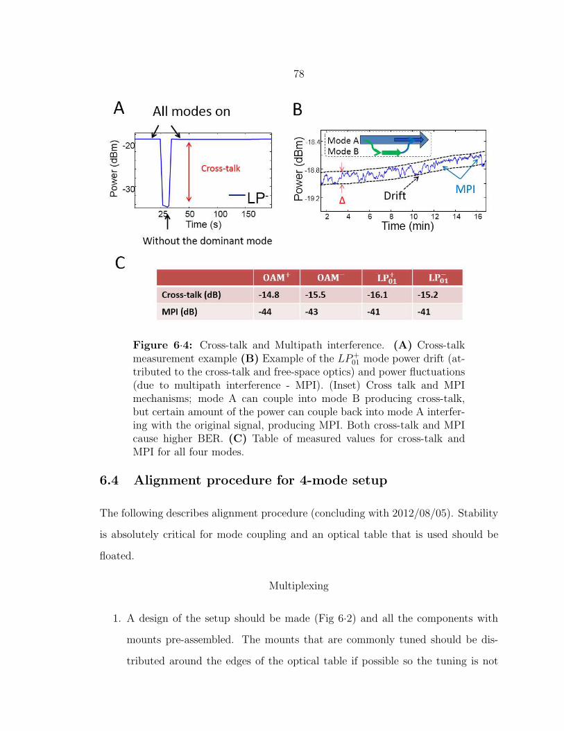
78

Figure 6·4: Cross-talk and Multipath interference. (A) Cross-talkmeasurement example (B) Example of the LP+

01 mode power drift (at-tributed to the cross-talk and free-space optics) and power fluctuations(due to multipath interference - MPI). (Inset) Cross talk and MPImechanisms; mode A can couple into mode B producing cross-talk,but certain amount of the power can couple back into mode A interfer-ing with the original signal, producing MPI. Both cross-talk and MPIcause higher BER. (C) Table of measured values for cross-talk andMPI for all four modes.

6.4 Alignment procedure for 4-mode setup

The following describes alignment procedure (concluding with 2012/08/05). Stability

is absolutely critical for mode coupling and an optical table that is used should be

floated.

Multiplexing

1. A design of the setup should be made (Fig 6·2) and all the components with

mounts pre-assembled. The mounts that are commonly tuned should be dis-

tributed around the edges of the optical table if possible so the tuning is not

79

Figure 6·5: Drift and MPI of all four modes.

strenuous for the user. At this point, one should also think about the future

packaging if needed.

2. Attach and collimate the 4 input channels (Fig 6·2) using IR cards.

3. (Course alignment) Place the mirror (M) instead of the proximal end of the

coupling fiber, and image the beam onto the camera at the camera position 1

(see Fig. 4·8A). Turn on all the channels and mark ROI for each of them. Tune

the channel mirrors until the channel beams more or less overlap.

4. (Fine alignment and astigmatism) Align the two mirrors of each channel to re-

move astigmatism. This is done by constantly scanning z-translation (focusing)

back and forth and adjusting one mirror, then the other. All the beams should

now overlap precisely without any astigmatism.

5. (Back-transmission) Remove mirror (M) and insert the vortex fiber. Distal

end of the vortex fiber should be free-space coupled into SMF (using splicer)

(note: do not splice the fibers to avoid offset coupling, even tiny amount can

be detrimental). Send the light through the distal end of the vortex fiber and

80

observe the so-called back-transmission at the camera position 1 (see Fig. 4·8A)

(note: all the mode channels should be turned off). Record the ROI. Adjust

the free-space offset coupling between SMF and a vortex fiber so only LP01 is

excited.

6. Turn off the SMF light source and turn back on the channels. Look at the back-

reflection from the vortex fiber and move the translation stage until overlap with

the ROI (recorded in the previous step) has been achieved.

7. Adjust pitch and x-translation of the back-transmission beam to remove astig-

matism caused by the fiber end-face tilt.

8. Repeat for yaw and y-translation.

9. Remove the side of the distal end of the vortex fiber attached to the source,

cleave it and image it (camera position 2, see Fig. 4·8A).

10. Adjust the zoom of the vortex fiber as well as fine tune the collimation for

optimal power coupling.

Demultiplexing

1. Prepare the optical components and mounts using the layout in Fig. 6·2.

2. Collimate the beam at the distal end of the vortex fiber (use the camera if a

signal is too weak).

3. Attached the distal end of the SMF that you want to couple into and look at

the back transmission on the IR card.

4. Using an IR card and a two mirrors alignment procedure, couple the light into

the fibers (note: two mirrors alignment procedure requires placing the IR card

81

on one of the mirrors first, then adjusting yaw and pitch, repeating the procedure

for the other mirror until convergence in alignment is achieved).

5. When reasonable alignment is achieved, small amount of power should be de-

tected at the SMF output. Next, walk-in the beam by repeatedly adjusting x

translation of the SMF stage and the yaw of the mirror closer to the coupling

stage. Repeat for the y-translation and the pitch angle. Guiding the beam into

the fiber at the proper angle is critical to achieve good coupling.

82

Chapter 7

OAM Transmission

In this chapter we present results of the systems experiments (i.e. data transmis-

sion using the 4-mode OAM-MDM setup described in the previous chapter (Ch. 6).

Four modes include two l = ±1 OAM modes multiplexed with the two fundamen-

tal polarization-multiplexed s = ±1 modes. We first briefly describe the basics of

data modulation formats and error-correction methods that we use. We then present

results of the two system experiments that performed:

• 4-mode OAM-MDM at single-wavelength (Bozinovic et al., 2012b)

• 2-mode OAM-MDM using 10-channel WDM (Yue et al., 2013)

Using coherent detection and bit-error-rate (BER) measurement that, we demonstrate

successful data transmission at 400Gbit/s using four OAM modes at a single wave-

length, over 1.1 km of fiber. Furthermore, we achieve data transmission at 1.6Tbit/s

using 10 wavelengths and two OAM modes (Bozinovic et al., 2012b).

7.1 Brief introduction in communication systems

From the very beginnings of communication systems, the desire for higher transmis-

sion capacities and, at the same time, the drive to reuse the existing transmission

channels, have fueled the advancements of data modulation formats. First modula-

tion formats were based of on-off keying, where bit of information was encoded in the

amplitude of the electric signal (’1’ when there is light and ’0’ for no light) (Fig. 7·1).

83

Later on, modulation formats started using frequency (or phase) of electric field to

encode information (see frequency and phase shift keying in Fig. 7·1). Today, myriad

Figure 7·1: Basic modulation formats using amplitude and phase odthe field. Non-return to zero (NRZ) denotes that signal doesn’t goto zero between two bits that both carry ’1’. With permission fromWikipedia, c© Creative Commons.

of advanced modulation formats exists depending on capabilities of particular trans-

mission systems, mainly separated into intensity and phase modulation groups (Fig.

7·2) (Winzer and Essiambre, 2006). While intensity modulation formats are typically

detected directly Fig. 7·3 (A), the phase-modulation formats require a reference beam

(also called local oscillator - LO) Fig. 7·3 (B). Not taking into account the nonlinear

effects of a fiber, a capacity (C) of any channel (with direct or coherent detection) is

C = Blog2(1 + SNR), where B is the bandwidth B and SNR is the signal-to-noise-

ratio in the channel (Shannon, 1948). In the case of direct-detection, it can be shown

that the capacity is restricted with the SNR of the light source. However, in the case

of coherent-detection, the SNR of the channel is predominantly determined by the

SNR of the LO. In a nutshell, due to the fact that LO power does not suffer from

the losses as much as the signal from the other end of the fiber, coherent-detection

approach has the advantage over direct-detection, and is becoming a predominant

84

Figure 7·2: Advanced modulation formats (Winzer and Essiambre,2006). For us most important formats is differential quadrature phaseshift keying (DQPSK) that we use in our systems experiment. For fulllist of acronyms consult (Winzer and Essiambre, 2006). With permis-sion from (Winzer and Essiambre, 2006), c© IEEE.

detection method today. While the description of the modulation formats in Fig. 7·2

Figure 7·3: Direct (A) vs Coherent (B) modulation formats. Withpermission from Wikipedia, c© Creative Commons.

is beyond the scope of this work, we focus on one that we used for our experiments,

namely, quadrature phase shift keying (QPSK). In essence, QPSK is an example of a

four-state system (also used terms for states are levels or symbols). What this means

is that both transmitter (Tx) and receiver (Rx) can send and/or receive four possible

states. For each state they agree on a bit combination, for example, ’00’, ’01’, ’10’

85

and ’11’. In an example of an intensity modulation, a laser with four levels of power

use say 0W to transmit ’00’, 1W to ’01’, 2W to ’10’ and 3W to ’00’. In the case of

QPSK, four levels are in fact encoded in four different phases of a wave. For example,

a wave with frequency fc,

sin(2πfct + (2n− 1)π

4), n = 1, 2, 3, 4 (7.1)

can have four different phases π/4, +3π/4, 5π/4 and +7π/4, for n = 1, 2, 3, 4. If the

receiver can detect the phase of the wave, it can recover the bit sequence. We briefly

note that in addition to 4-level QPSK, 16-level modulation can be used in which case it

is called 16-quadrature amplitude modulation (16-QAM). For a detailed explanation,

implementation as well as different variants of the QPSK and 16-QAM method, we

recommend (Ip et al., 2008).

Our QPSK concept is shown on Fig. 7·4 (A-B). A sender can encode information

in a π/4, +3π/4, 5π/4 and +7π/4 phase of a beam, and a receiver can decode the bits

as ’11’, ’01’, ’00’ and ’11’, respectively. Due to dispersion, polarization-dependant loss

and/or gain, and nonlinear effects, the detected phase can be slightly different from

the one being sent. If the difference is too large, an erroneous bit can be received,

and a bit-error-rate (BER) will increase. In telecommunication, an eye pattern, also

known as an eye diagram, is an oscilloscope display in which a digital data signal from

a receiver is repetitively sampled and shown on a vertical scale, while the data rate is

used to trigger the horizontal sweep. In other words, it represents the synchronized

superposition of all possible realizations of the signal of interest viewed within a

particular signalling interval. It is so called because, for several types of coding, the

pattern looks like a series of eyes between a pair of rails. It is an experimental tool for

the evaluation of the combined effects of channel noise and intersymbol interference

on the performance of a pulse-transmission system. Typical noiseless and noisy case

86

Figure 7·4: Concept of quadrature phase shift keying (QPSK) and eye-diagram for bit-error-rate testing. (A) Ideal QPSK constellation. Asender can encode information in a π/4, +3π/4, 5π/4 and +7π/4 phase,corresponding to 11, 01, 00 and 11 bit combination. Therefore, a phasecan carry 4 possible states. (B) Noisy case. A phase of light can sufferchanges due to fiber impediments, and in the noisy case, wrong phasecan be detected, and errors in transmission can occur. (C) Conceptof an eye diagram in the case of intensity modulation. Train of pulsescarrying bits can be overlapped to create an eye-shaped diagram. (C)In a noisy case, distortion can cause ”eye-closing” introducing errors intransmission. Similar eye diagram can be observed in the QPSK case.C and D with permission from Wikipedia, c© Creative Commons

of an eye diagram is shown in Fig. 7·4 (C-D).

Depending on a type of application, different levels of errors are allowed in the

system. In a typical communication system, a BER level on the order of 10−12 is

tolerable. However, this level can be quite challenging to achieve using the methods

we have explained, and in addition to the physical means of sending information,

so-called forward-error-correction (FEC) codes are used. The central idea is that the

sender encodes a message in a redundant way. The redundancy allows the receiver

87

to detect a limited number of errors that may occur anywhere in the message, and

often to correct these errors without retransmission. This note that FEC gives the

receiver the ability to correct errors without needing a reverse channel to request

retransmission of data, but at the cost of a fixed, higher forward channel bandwidth.

An example of a FEC code is the Hamming (7,4) code (Hamming, 1950). This

code encodes 4 bits of data into 7 bits by adding 3 parity bits. If the error of any one

bit out of 7 would occur, the sequence can detect the error, which can be corrected.

If the medium is too noisy so that 2 out of 7 bits are flipped, error will be detected.

However, the likelihood for two bits to be flipped is much smaller then in the case of

one. The redundancy of the code can be described with the ratio of data bits vs total

number of bits (in the case of Hamming (7,4) code this rate is 4/7 = .571). Today,

FEC codes with much smaller redundancy has been implemented such as: convolution

code, Low-density parity-check (LDPC), and many others. In our system, we used

FEC that can tolerate BER with the threshold of 3.8 × 10−4. Detailed explanation

of the FEC codes goes beyond the scope of this dissertation (for more details we

recommend (Freeman, 2002).

With basic knowledge of modulation formats and FEC codes we now present

results of fiber-based OAM-MDM experiments in the vortex fiber.

7.2 4-mode OAM-MDM

Here we demonstrate OAM-MDM data transmission feasibility of the 4-mode system

described in Ch. 6, by sending 50 GBaud (1 Baud = 1 symbol/s), QPSK data, at

a single wavelength, and over 4 mode-channels. The detailed experimental OAM-

MDM setup is shown on Fig. 7·5. For the single wavelength experiments, a CW-ECL

operating at 1550 nm was first modulated using a 50 GBaud QPSK signal, and

subsequently split into four arms that were delayed sufficiently to obtain four de-

88

Figure 7·5: Systems experiment setup: signal from the laser or WDMsource is modulated, amplified using an erbium doped fiber amplifier(EDFA), filtered using a band pass filter (BPF) and split into four individ-ual fiber arms (two in the case of the WDM experiment). Two of the armswere converted into OAM modes using the input SLM. Two fundamentalmodes were also collinearly aligned with the two OAM modes using a beam-splitter, and all four modes were coupled into the fiber. After propagation,the modes are demultiplexed sequentially and sent for coherent detectionand offline digital signal processing (DSP). Acronyms: ADC - analog digitalconvertor, Att - attenuator, FM - flip mirror, LO - local oscillator, OC -optical coupler, (N)PBS: (non)-polarizing beam-splitter, PBC - polarizationbeam combiner, PC - polarization controllers, PC-SMF - polarization con-troller on SMF, PC-VF - polarization controller on vortex fiber. OC: opticalcoupler, (N)PBS: (non)-polarizing beam-splitter, PBC: polarization beamcombiner, PC: polarization controller

correlated data channels (two for the WDM experiments in the next section). Two

of the four channels were converted into the OAM± modes (modes A and B) using

reflection off fork-holograms of topological charge ±1, created using the LCOS-SLM

(X10468-8, Hamamatsu). The other two, LP01, modes were left unchanged (modes

C and D). A 6-axis fiber stage positioner (Thorlabs, MAX601D) was used for input

coupling into the vortex fiber. Precise optical alignment enabled avoiding any offset

coupling, which can otherwise introduce strong crosstalk (offset coupling of < 50nm

89

was necessary and achieved). We found that the incident angle (of light on the fiber

facet) to also be important for input coupling, but less critical than the offset. Fiber

coupling losses were 0.7dB for the LP01 and 1.1dB for the OAM modes.

After alignment, the four polarization controllers at the channel inputs (A, B, C

and D on Fig. 7·5) would be adjusted first to equalize the output channel powers.

Next, the polarization controller on the vortex fiber (PC-VF in Fig. 7·5) would be

adjusted to obtain OAM± states at the vortex fiber with the smallest cross-talk (a

minimum value of -20dB was obtained). Finally, the polarization controller on the

input SMF (PC-SMF) was adjusted to obtain LP±

01 modes at the output with the

smallest crosstalk (< −30dB was achieved). Note that we did not necessarily have

LP±

01 states at the channel inputs (C, D) but rather states with arbitrary polariza-

tions; however, OAM± states were ensured at both input and output. The vortex

fiber spool was thermally isolated using a custom-made Styrofoam box. Polariza-

tion controllers needed adjustments in roughly one-hour increments to account for

components drifts and temperature fluctuations. We note that automated polariza-

tion controller feedback corrections are commonly used techniques in conventional

polarization-division multiplexed (PDM) systems (Sunnerud et al., 2002).

Figure 7·6 shows constellation diagrams in the case of the 4-mode OAM-MDM ex-

periment in the single-channel as well as all-channel case, using 50 GBaud non-return-

to-zero (NRZ) QPSK at 1550 nm. BERs are measured for two cases: when only one

channel is used for data transmission (single-channel case), and when all four channels

are simultaneously populated with distinct (decorrelated) data-streams (all-channels

case) (Fig. 7·7 B). In the single-channel case, the largest received power penalty

for achieving a BER of 3.8 × 10−3 (the threshold BER level at which forward-error-

correction (FEC) algorithms ensure error-free data transmission) is 2.5 dB, mainly

due to channel MPI. In the all-channel case, this largest power penalty increased to

90

Figure 7·6: Constellation diagrams in the case of 4-mode OAM-MDM,with 50 GBaud NRZ-QPSK, λ = 1550nm, for the single-channel, andall-channel cases. Note the larger distortion of the constellations in theall-channel case.

4.1 dB, mainly due to channel cross-talk. In the latter case, a total transmission

capacity at 400 Gbit/s below the FEC limit is achieved.

7.3 2-mode OAM-MDM

In addition to the single wavelength demonstration, we used WDM to further extend

the capacity of our system (Fig. 7·8 A). According to mode coupling theory (Mar-

cuse, 1974), cross-talk in coherent systems depends on a beam phase that, in turn,

depends on the wavelength. Thus, optimizing our system to yield two orthogonal,

pure OAM± states at one wavelength implies that, at other wavelengths, the OAM±

states will, to a certain extent, couple into each other. A more advanced transmit-

ter with individual wavelength channel polarization control could, in principle, be

used to mitigate this effect. In addition, extraneous contributory factors such as the

wavelength dependence of the SLM and other free-space optical components can also

affect the cross-talk. For these reasons, only two OAM modes and 10 WDM channels

(from 1546.64 to 1553.88 nm) are chosen for our WDM experiment. (the boxed region

in Fig. 7·8 B), illustrating wavelengths at which crosstalk was low). Reduction to

91

Figure 7·7: Data transmission experiments. (A) Block diagram of 50× 2 Gb/s QPSK signal transmission over a single wavelength carrying 4modes in the vortex fiber. (B) Measured BER as a function of receivedpower for the single-channel (SC) and all-channels (AC) transmissioncase.

two modes allowed us to choose a more complex modulation format (16-quadrature

amplitude modulation) for data transmission, yielding higher spectral efficiency, al-

beit with a lower baud rate of 20 GBaud. While the BER of the two modes varied

somewhat due to crosstalk (Fig. 7·8 C), transmission of 20 channels (OAM-MDM and

WDM), resulted in a total transmission capacity of 1.6 Tb/s under the FEC limit.

Figure 7·9 shows additional results of the system experiment with 2-OAM modes,

10 wavelengths and 16-QAM signal modulation. The optical spectra of the modulated

signal just before the input at the fiber, and after transmission in the OAM+ mode

followed by the demux are plotted in Fig. 7·9 (A). We can see that all WDM channels

92

Figure 7·8: (A) Block diagram of 20×4 Gb/s 16-QAM signal trans-mission over 10 wavelengths carrying 2 modes in the vortex fiber. (B)Measured crosstalk between OAM± modes as a function of wavelength.(C) BER as a function of wavelength for OAM± modes in the WDMsystem.

have a 25dB OSNR after demultiplexing. Figure 7·9 (B) shows constellations for a)

16-QAM back-to-back (B2B) data transmission, b) OAM+ mode at 1550.64 nm w/o

crosstalk (XT) (one wavelength is on, one mode is on), c) OAM+ mode at 1550.64

nm w/ WDM XT (10 wavelengths are on, one mode is on), and d) OAM+ mode for

WDM source w/ all XT (10 wavelengths are on, two mode are on). Note the gradual

increase in distortion of the constellations as wavelengths and modes are added to

the fiber. Figure 7·9 (C) shows measured BER curves for the OAM modes at 1550.64

nm, in the WDM case, as a function of received power. At the optimal wavelength,

crosstalk for the two OAM modes was -21.4 dB and -20.2 dB, respectively. We can see

93

that the BER for the mode OAM+ is slightly better than that for the mode OAM−

mode, mainly due to differences in alignment of the optical components. At the FEC

limit (3.8 × 10−3 according to the ITU-T Recommendation G.975.1, Appendix I.9,

2004), the average power penalty of mode OAM+ and OAM− for the cases w/o XT,

w/ WDM XT and w/ all XT are 1.8 dB, 2.4 dB and 4.55 dB, respectively.

Figure 7·9: Additional experimental results of the 2-OAM modes, 10wavelengths, 16-QAM systems experiments. (A) Spectrum of the mod-ulated signal at the output of the WDM 16-QAM Tx, and spectrumof the OAM+ mode at the receiver after demultiplexing. (B) Constel-lations of 16-QAM modulation for the demultiplexed OAM+ mode at1550.64 nm, for several cases (without and with crosstalk). (C) BER asa function of received power at 1550.64 nm, for B2B, and OAM modeswithout and with XT from WDM channels or the other OAM mode.

Despite the higher cross-talk between the two OAM± modes as we move away from

the optimal wavelength, spiral interference patterns were observed throughout the

1540−1570nm wavelength range. Figure 7·10 demonstrates this for the OAM+ case;

for brevity, only a few wavelengths, spaced in 10pm, 100pm, 1000pm and 10nm steps

are shown (as before, a CW-ECL with 100 kHz linewidth and a 60 µs camera exposure

time was used for this measurement). The OAM+ mode purity (and hence spiral

quality) degrades for some intermediate wavelengths, but the fact that it generally

maintains a spiral pattern is indicative of a substantially pure OAM mode over a

94

30-nm spectral range.

Figure 7·10: Spiral interference patterns, showing helical phase, ofthe OAM+ mode at different wavelengths for the same vortex fiberconditions (no polarization controller adjustments). (A-D) Spiral pat-terns for the wavelengths spaced in 10pm, 100pm, and 1000pm. (E-H)Spirals for the wavelengths spaced in 10nm.

95

Chapter 8

Conclusion

In this dissertation we have studied in detail a new type of fiber, called vortex fibers,

that has a potential to increase the capacity of future communication links. We first

theoretically studied modes of a MMF with an arbitrary index profile, and proved

that a linear combination of vector modes HEevenl+1,m and HEodd

l+1,m, with π/2 phase

shift among them, poses an OAM of topological charge l. We identified small effective

index separation as the reason for instability of OAM modes in conventional fibers.

Numerical methods were used to investigate the mode properties in vortex fibers,

showing increase in separation of the effective and group indices in vortex fibers. We

have then build a setup using stress-induced microbend gratings to experimentally

verify the numerical findings and observed good agreement. Using imaging methods

we then qualitatively confirmed that OAM modes are indeed created in vortex fibers

by recording their characteristic doughnut-shaped intensity profiles, and spiral-shaped

phase profiles.

Next we studied in details three methods for OAM mode generation: one based

on stress-induced microbend gratings, second one based on a carbon-dioxide (CO2)-

laser induced fiber gratings, and the third one based on free-space coupling using

liquid-crystal on silicon spatial-light-modulator (LCoS SLM). We have shown that

the microbend gratings are significantly polarization sensitive due to stress-induced

birefringence but can create OAM modes that are 25dB strong (without tapers) and

35dB strong (with tapers). Setup capable of making CO2 gratings was built and

96

results have shown less polarization sensitivity that in the case of microbend gratings.

However the generation technique has a limit of creating only 12dB strong OAM

modes (without tapers). We also built a setup using SLM as a generation method

which as capable of creating 20dB strong OAM modes over tens of nanometers range.

In order to quantitatively measure fiber modal content and hence purity of OAM

modes in vortex fibers two methods were developed: the ring method and regression

analysis method Both methods are based on imaging and spatial Fourier analysis of

the intensity images. We showed that the OAM states with ≈ 97% purity can be

generated after 20m of vortex fiber, and ≈ 90% purity after 1km.

To demonstrate that OAM modes supported in vortex fiber can be used for MDM,

we have build a 4-mode multiplexing setup based on the SLM mode generation. We

have tested the setup for the cross-talk and MPI of the mode-channels as well as

sensitivity to alignment, polarization and wavelength.

Finally, we demonstrated a 4-mode OAM-MDM by sending data over the 4-modes

of vortex fiber at a single wavelength and at 400Gbit/s, with bit-error-rates below

the FEC limit of 3.8 × 10−3. We used WDM to expand the capacity of the system

to 1.6Tbit/s data transmission speed (SE of 1.6 bit/s/Hz). Our results indicate

that simple, low-complexity DSP coherent detection methods can be used to achieve

4-mode OAM-MDM. These demonstrations show the potential of OAM-MDM in

special types of fibers, and support further investigations of specialty MMFs for future

transmission systems.

8.1 Observations

In this section we address some of the limitations of the OAM-MDM technique pre-

sented in this dissertation, as well as offer some of the ideas for the future investiga-

tions regarding vortex fiber and OAM-MDM in general.

97

Multiplexing: Our single wavelength demonstrations on vortex fiber was conducted

on 1.1km long fiber using QPSK modulation and 50 GBaud rate. The very first result

that was obtained was achieving only 10 GBaud rates, with higher rates resulting in

transmission above FEC threshold. This indicates that multiplexing crosstalk as

critical in our non-MIMO-based coherent detection. Hence, it is our belief that the

multiplexing setup has certain room for improvement.

Long length: Experiments on longer lengths could be done though in linear sys-

tems, the figure of merit is the bandwidth-distance product, not just one or the other

quantity (in our current systems this product was 1.45Tbit/s/km).

Polarization controllers: In our systems experiment demonstrations, polarization

controllers’ adjustments were done every hour in order to minimize the cross-talk.

This adjustments process is standard in today’s advanced digital coherent systems,

where the electric fields at the input and the output of the channel are available to

DSPs at both transmitter and receiver, which enables the use of arbitrary impairment

precompensation and postcompensation algorithms.

SE: In our case we have used 100GHz spectral grid which led to SE of 1.6 bit/s/Hz

after 1.1km. A close inspection of Fig. 7·9A, shows that 50GHz spacing could

be potentially used, to double the higher SE. Using more advanced transmitters

with individual wavelength channel polarization controls would allow cross-talk to

be minimized for each wavelength channel independently, enabling potentially higher

bandwidth utilization. However, increase in capacity obtained this way does not

increase the SE of our system.

MIMO: Because of intensive DSP requirements, no MIMO-based data transmis-

sion demonstrations so far have been demonstrated in real time. While large pro-

cessing power would in principle be possible to enable real time processing, power

consumption of such a system would be largely inefficient for today’s standards. Just

98

as a comparison, an estimate of 80W is used for the simplest 2x2 MIMO processing

in a commercial, polarization division multiplexed systems (PDM) (Frankel, 2013)1.

In addition, complexity of MIMO doesn’t scale linearly with number of modes. Using

simulations Arik et al. have predicted that, per mode, MIMO complexity is a factor

1.4, 1.7, 2.2, 2.8 times higher for number of modes being 6, 12, 20, 30 then for PDM in

standard SMF (Arik et al., 2013). Hence, this complexity is additional to the N2 com-

plexity increase, where N is the number of modes. Another drawback of MIMO could

be that it requires very low differential group delay (Ryf et al., 2012), indicating that

nonlinear effects might be increased due to increased cross-phase modulation ((Es-

siambre and Tkach, 2012) p.1050). Nevertheless, MIMO DSP systems are the only

MMFs systems, capable of performing high-speed transmission at metro- (∼ 10km)

and long-haul (45− 70km) lengths today. In order to achieve scaling required in the

future, vortex fibers would have to support higher number of modes that 4, and at

least 4x4 MIMO within a family of modes need to be considered (Ryf et al., 2012).

New generation of fibers that, similarly to the vortex fiber, aim to reduce cross-talk

among mode groups is currently active area of research (Gregg et al., 2013).

Adaptive optics feedback (AOF) methods: We find the adaptive optics methods

(Carpenter et al., 2012) very interesting. One downside of this method is the require-

ment for a two-dimensional intensity distribution at the fiber output, necessary for

feedback. Though not impossible, this approach might require significant atypical re-

quirements from the future systems for it to be deployed (for example a signal would

need to be tapped and image onto high speed camera). Though computationally in-

tensive, it would be interesting to quantify how would this correction affect the reach.

According to (Carpenter et al., 2012), timescale of 50 µm, graded index, conventional

MMF change is on the order of minute and we expect vortex fiber to be more stable

1Due to processor cooling, all data centers in the world combined contribute to roughly 0.4% ofworld’s power consumption (Vuckovic, 2013).

99

in the respect. In addition, MMF used is graded index. Similar results have been

obtained for 2km and 8km, promising longer lengths would be possible (Carpenter

et al., 2013).

Reduce slope dispersion: In Ch. 3, we have found total dispersion (material +

waveguide dispersion) to be low in the C-band, however, with the relatively large

slope (Fig. 3·7B). A modified version of vortex fiber that will have reduce the slope

should be considered for WDM systems to mitigate the dispersion (typical dispersion-

shifted fibers are engineered to have total dispersion around 2 to 6 ps/nm/km in the

C-band, the zero dispersion being avoided due to enhanced nonlinear effects such as

FWM). In addition, we note that the modal dispersion is slightly different and design

that will equalize their dispersion should be investigated.

Loss: Loss in the vortex fiber of 1.3dB for LP01 is relatively high with respect to

conventional fibers, and could affect the SNR of the signal after long length propa-

gation, however, The loss in fibers can be caused by material absorbtion, linear and

nonlinear scattering, as well as macrobends and microbends (Smink et al., 2007). In

addition, anomalous loss was observed due to high refractive index difference (∆) in

core/cladding regions, and was attributed to draw-induced fluctuations of core radius

(Lines et al., 1999). Under certain assumptions, this anomalous loss was theoreti-

cally predicted to scale with ∆2. The fact that ∆ of 0.03 in the vortex fiber is quite

large, an order of magnitude larger then in SMFs, supports anomalous loss claim.

Nevertheless, it is possible that the current manufacturing vortex fiber method is not

optimized.

Mode dependant loss: Modal dependant loss (i.e. excess loss) causes impediment

in the PDM and MDM systems (Sunnerud et al., 2002). This effect is predicted

theoretically and can be explained by mode coupling theory where perturbations

have longitudinal spatial frequencies below the range required for mode coupling

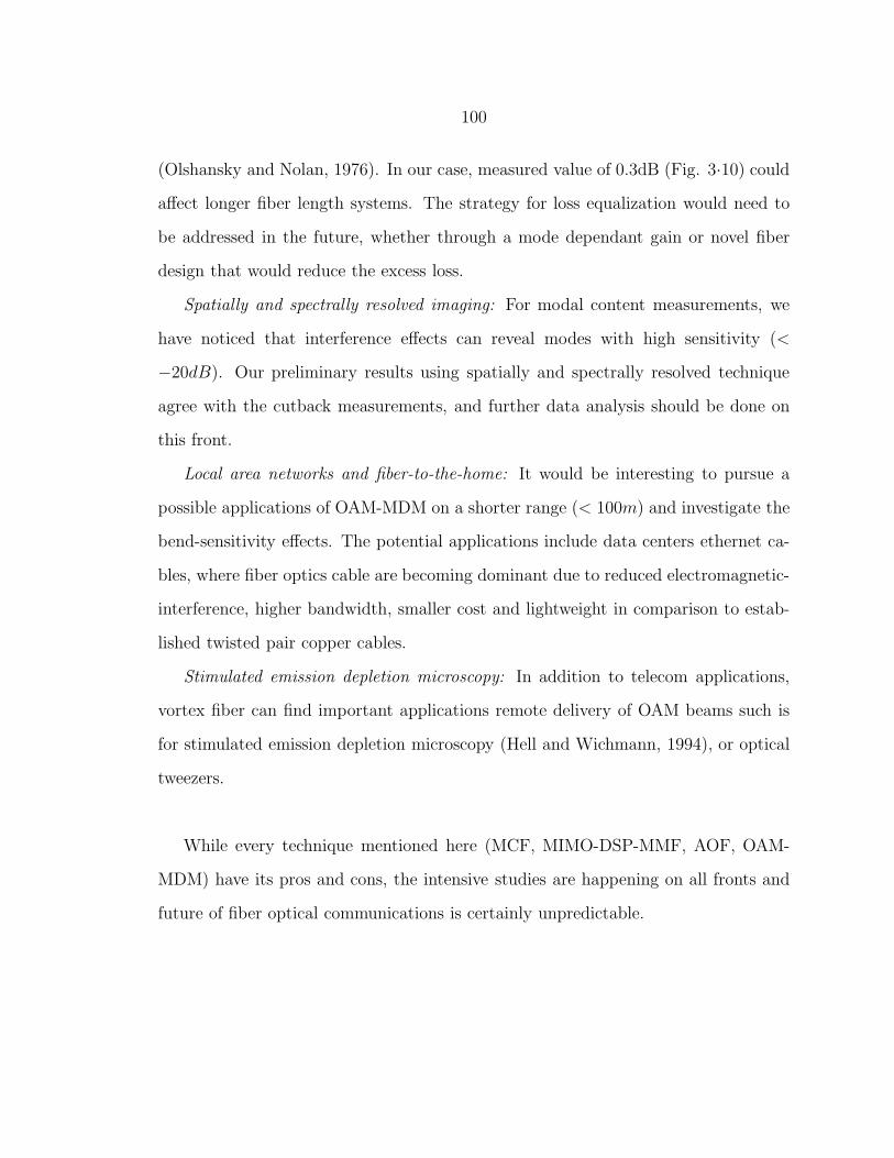
100

(Olshansky and Nolan, 1976). In our case, measured value of 0.3dB (Fig. 3·10) could

affect longer fiber length systems. The strategy for loss equalization would need to

be addressed in the future, whether through a mode dependant gain or novel fiber

design that would reduce the excess loss.

Spatially and spectrally resolved imaging: For modal content measurements, we

have noticed that interference effects can reveal modes with high sensitivity (<

−20dB). Our preliminary results using spatially and spectrally resolved technique

agree with the cutback measurements, and further data analysis should be done on

this front.

Local area networks and fiber-to-the-home: It would be interesting to pursue a

possible applications of OAM-MDM on a shorter range (< 100m) and investigate the

bend-sensitivity effects. The potential applications include data centers ethernet ca-

bles, where fiber optics cable are becoming dominant due to reduced electromagnetic-

interference, higher bandwidth, smaller cost and lightweight in comparison to estab-

lished twisted pair copper cables.

Stimulated emission depletion microscopy: In addition to telecom applications,

vortex fiber can find important applications remote delivery of OAM beams such is

for stimulated emission depletion microscopy (Hell and Wichmann, 1994), or optical

tweezers.

While every technique mentioned here (MCF, MIMO-DSP-MMF, AOF, OAM-

MDM) have its pros and cons, the intensive studies are happening on all fronts and

future of fiber optical communications is certainly unpredictable.

101

Appendix

A1. Polarization dependence of beamsplitters and

mirrors

Polarization dependance of mirrors and beamsplitters can affect the Ring analysis

and give erroneous results of mode purity. In this section, we wanted to study po-

larization dependence of three devices: 45o angled mirror (Thorlabs, BB1-E04), and

two beamsplitters (Thorlabs BS015 and Newport 10BC17MB.1).

The setup is shown on Figure 8·1. Light from a single mode fiber is sent through a

polarizer and then through the device under test. The polarization is then measured

using polarimeter (comprised of a polarizer and a quarter wave plate, and a camera).

To determine polarization, four images with certain orientation of a polarimeter are

acquired (Berry et al., 1977).

Polarization of the three devices was measured for three different positions of a

polarizer: horizontal, vertical and 45o degrees linearly polarized states (results are in

the 04/18/2012 folder). Polarization ellipses for certain points clearly indicate that

beamsplitters affect the polarization state after reflection (Fig. 8·2).

In particular, a phase delay is introduced between two polarizations in the case of a

45o degrees linearly polarized state (x+ y state becomes x+eiΓy). Mirror performance

was better (Fig. 8·3).

Note that if a polarizer is placed after the beamsplitter, the effect of phase delay

won’t play such a big role, as the phase delay of a single polarization will not be

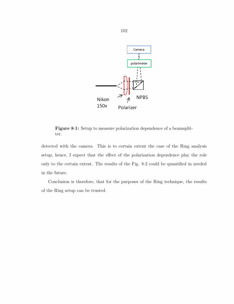
102

Figure 8·1: Setup to measure polarization dependence of a beamsplit-ter.

detected with the camera. This is to certain extent the case of the Ring analysis

setup, hence, I expect that the effect of the polarization dependence play the role

only to the certain extent. The results of the Fig. 8·2 could be quantified in needed

in the future.

Conclusion is therefore, that for the purposes of the Ring technique, the results

of the Ring setup can be trusted.

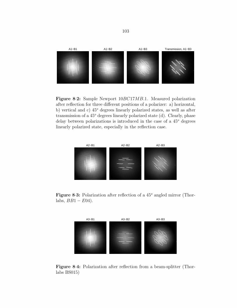
103

A1−B1

A1−B2

A1−B3

Transmission, A1−B3

Figure 8·2: Sample Newport 10BC17MB.1. Measured polarizationafter reflection for three different positions of a polarizer: a) horizontal,b) vertical and c) 45o degrees linearly polarized states, as well as aftertransmission of a 45o degrees linearly polarized state (d). Clearly, phasedelay between polarizations is introduced in the case of a 45o degreeslinearly polarized state, especially in the reflection case.

A2−B1

A2−B2

A2−B3

Figure 8·3: Polarization after reflection of a 45o angled mirror (Thor-labs, BB1− E04).

A3−B1

A3−B2

A3−B3

Figure 8·4: Polarization after reflection from a beam-splitter (Thor-labs BS015)

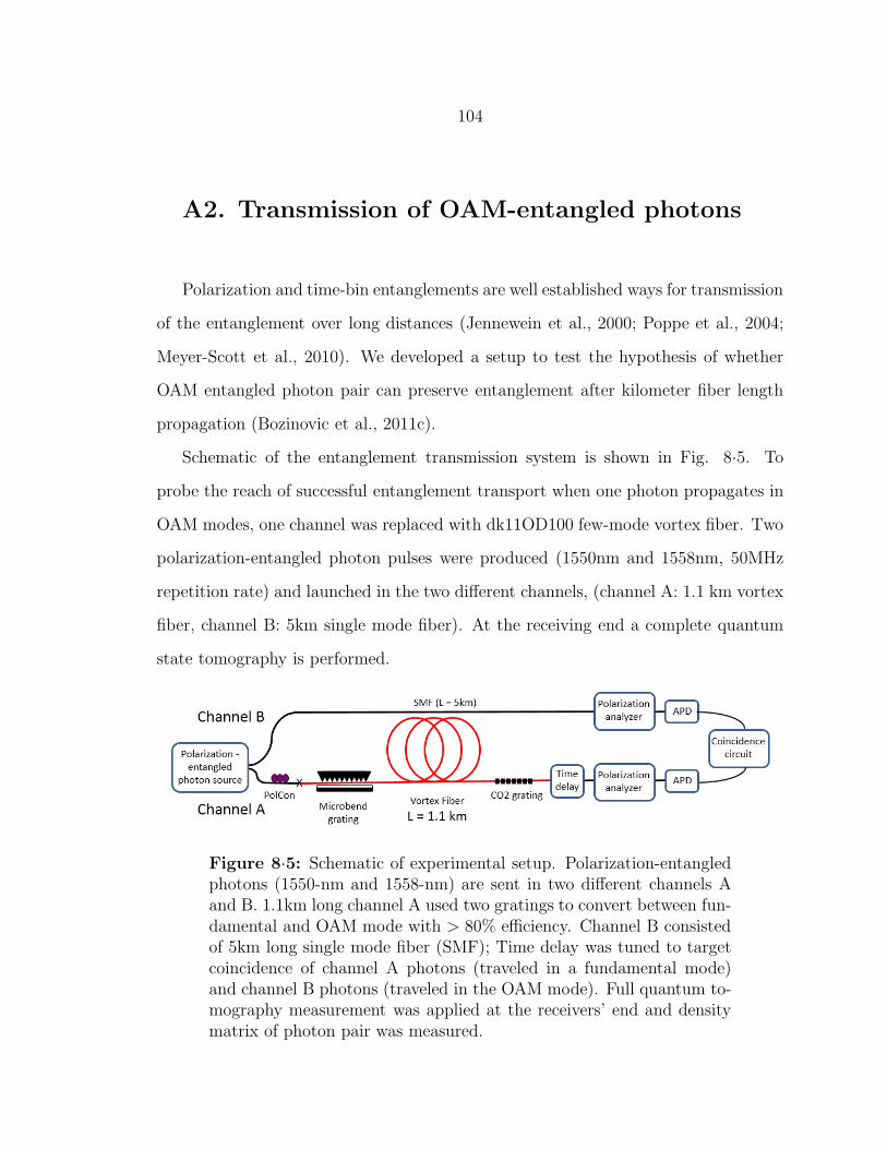
104

A2. Transmission of OAM-entangled photons

Polarization and time-bin entanglements are well established ways for transmission

of the entanglement over long distances (Jennewein et al., 2000; Poppe et al., 2004;

Meyer-Scott et al., 2010). We developed a setup to test the hypothesis of whether

OAM entangled photon pair can preserve entanglement after kilometer fiber length

propagation (Bozinovic et al., 2011c).

Schematic of the entanglement transmission system is shown in Fig. 8·5. To

probe the reach of successful entanglement transport when one photon propagates in

OAM modes, one channel was replaced with dk11OD100 few-mode vortex fiber. Two

polarization-entangled photon pulses were produced (1550nm and 1558nm, 50MHz

repetition rate) and launched in the two different channels, (channel A: 1.1 km vortex

fiber, channel B: 5km single mode fiber). At the receiving end a complete quantum

state tomography is performed.

Figure 8·5: Schematic of experimental setup. Polarization-entangledphotons (1550-nm and 1558-nm) are sent in two different channels Aand B. 1.1km long channel A used two gratings to convert between fun-damental and OAM mode with > 80% efficiency. Channel B consistedof 5km long single mode fiber (SMF); Time delay was tuned to targetcoincidence of channel A photons (traveled in a fundamental mode)and channel B photons (traveled in the OAM mode). Full quantum to-mography measurement was applied at the receivers’ end and densitymatrix of photon pair was measured.

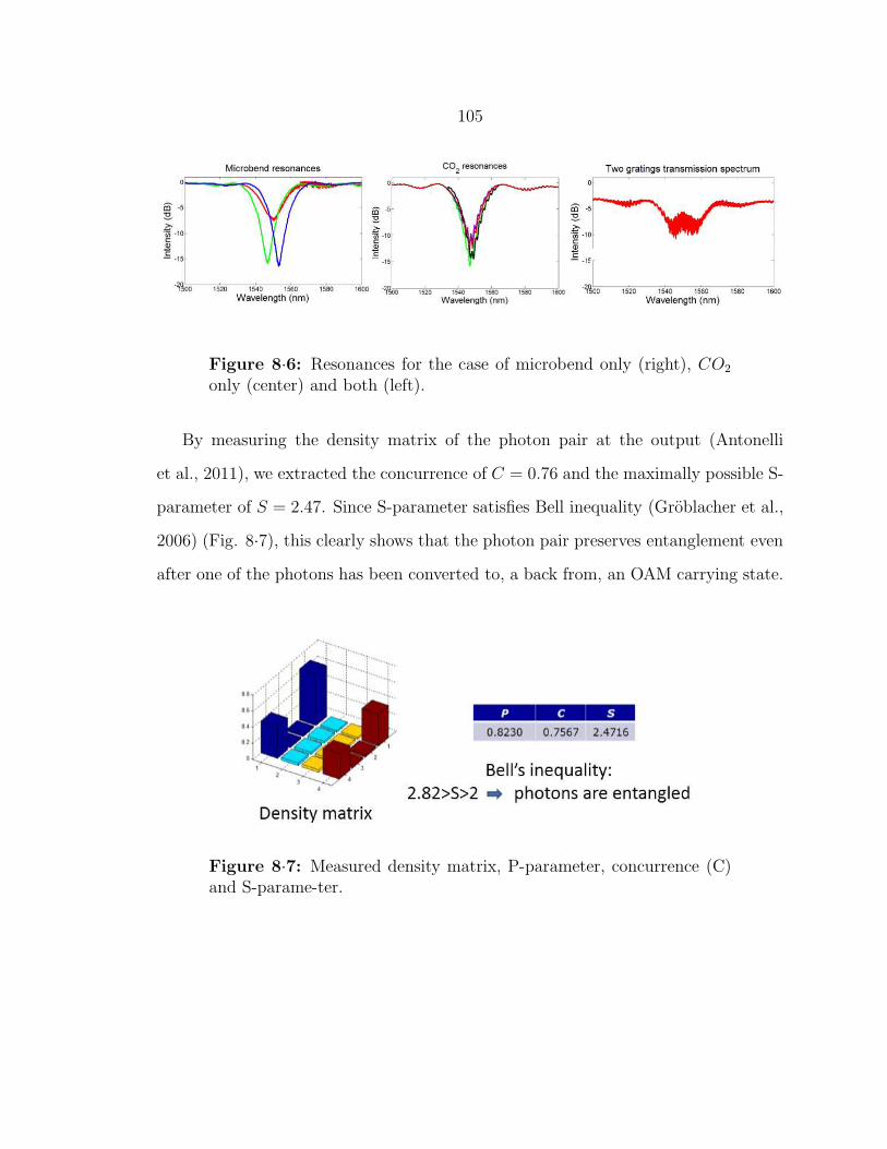
105

Figure 8·6: Resonances for the case of microbend only (right), CO2

only (center) and both (left).

By measuring the density matrix of the photon pair at the output (Antonelli

et al., 2011), we extracted the concurrence of C = 0.76 and the maximally possible S-

parameter of S = 2.47. Since S-parameter satisfies Bell inequality (Groblacher et al.,

2006) (Fig. 8·7), this clearly shows that the photon pair preserves entanglement even

after one of the photons has been converted to, a back from, an OAM carrying state.

Figure 8·7: Measured density matrix, P-parameter, concurrence (C)and S-parame-ter.

106

A3. Publication list

[1] N. Bozinovic, S. Golowich, P. Kristensen, and S. Ramachandran, ”Control of

orbital angular momentum of light with optical fibers,” Opt. Lett. 37, 2451-2453

(2012).

[2] N. Bozinovic, Y. Yue, Y. Ren, M. Tur, P. Kristensen, A. Willner, and S.

Ramachandran, ”Orbital Angular Momentum (OAM) Based Mode Division Multi-

plexing (MDM) over a Km-length Fiber,” in European Conference and Exhibition on

Optical Communication, OSA Technical Digest (online) (Optical Society of America,

2012), paper Th.3.C.6.

[3] N. Bozinovic, P. Kristensen, and S. Ramachandran, ”Are Orbital Angular

Momentum (OAM/Vortex) States of Light Long-Lived in Fibers?,” in Frontiers in

Optics 2011/Laser Science XXVII, OSA Technical Digest (Optical Society of America,

2011), paper LWL3.

[4] N. Bozinovic, S. Ramachandran, M. Brodsky, and P. Kristensen, ”Record-

length transmission of entangled photons with orbital angular momentum (vortices),”

in Frontiers in Optics 2011/Laser Science XXVII, OSA Technical Digest (Optical

Society of America, 2011), paper PDPB1.

[5] N. Bozinovic, P. Kristensen, and S. Ramachandran, ”Long-range fiber transmis-

sion of photons with orbital angular momentum,” in CLEO:2011 - Laser Applications

to Photonic Applications, OSA Technical Digest (CD) (Optical Society of America,

2011), paper CTuB1.

[6] N. Bozinovic, C. Ventalon, T. Ford, and J. Mertz, ”Fluorescence endomi-

croscopy with structured illumination,” Opt. Express 16, 8016-8025 (2008).

[7] N. Bozinovic, C. Ventalon, T. Ford, and J. Mertz, ”Fluorescence Endomi-

107

croscopy with Out-of-Focus Background Rejection,” in Biomedical Optics, OSA Tech-

nical Digest (CD) (Optical Society of America, 2008), paper BTuF57.

[8] Y. Yue, N. Bozinovic, Y. Ren, H. Huang, M. Tur, P. Kristensen, S. Ramachan-

dran, and A. Willner, ”1.6-Tbit/s Muxing, Transmission and Demuxing through 1.1-

km of Vortex Fiber Carrying 2 OAM Beams Each with 10 Wavelength Channels,”

in Optical Fiber Communication Conference/National Fiber Optic Engineers Confer-

ence 2013, OSA Technical Digest (online) (Optical Society of America, 2013), paper

OTh4G.2.

[9] S. Golowich, N. Bozinovic, P. Kristensen, and S. Ramachandran, ”Complex

mode amplitude measurement for a six-mode optical fiber,” Opt. Express 21, 4931-

4944 (2013).

[10] S. Golowich, P. Kristensen, N. Bozinovic, P. Gregg, and S. Ramachandran,

”Fibers Supporting Orbital Angular Momentum States for Information Capacity Scal-

ing,” in Frontiers in Optics 2012/Laser Science XXVIII, OSA Technical Digest (on-

line) (Optical Society of America, 2012), paper FW2D.2.

[11] S. Golowich, N. Bozinovic, P. Kristensen, and S. Ramachandran, ”Vortex

Fiber Mode Amplitude Estimation,” in Conference on Lasers and Electro-Optics 2012,

OSA Technical Digest (online) (Optical Society of America, 2012), paper JTu2K.2.

[12] S. Ramachandran, N. Bozinovic, P. Gregg, S. Golowich, and P. Kristensen,

”Optical vortices in fibres: A new degree of freedom for mode multiplexing,” in

European Conference and Exhibition on Optical Communication, OSA Technical

Digest (online) (Optical Society of America, 2012), paper Tu.3.F.3.

[13] S. Santos, K. Chu, D. Lim, N. Bozinovic, T. Ford, C. Hourtoule, A. Bartoo, S.

Singh, and J. Mertz, ”Optically Sectioned Fluorescence Endomicroscopy with Hybrid-

Illumination Imaging through a Flexible Fiber Bundle,” in Advances in Imaging, OSA

Technical Digest (CD) (Optical Society of America, 2009), paper NWC3.

References

Abrishamian, F., Dragomir, N., and Morishita, K. (2012). Refractive index profilechanges caused by arc discharge in long-period fiber gratings fabricated by a point-by-point method. Applied optics, 51(34):8271–6.

Agrawal, G. P. (2010). Fiber-optic communication systems. Wiley, 4th edition.

Allen, L., Beijersbergen, M., Spreeuw, R., and Woerdman, J. (1992). Orbital angu-lar momentum of light and the transformation of Laguerre-Gaussian laser modes.Physical Review, 45(11):8185–89.

Andrews, D. (2008). Structured Light and Its Applications. Academic Press.

Antonelli, C., Shtaif, M., and Brodsky, M. (2011). Sudden Death of EntanglementInduced by Polarization Mode Dispersion. Physical Review Letters, 106(8):080404.

Arik, S., Askarov, D., and Kahn, J. (2013). Effect of mode coupling on signal process-ing complexity in mode-division multiplexing. Journal of Lightwave Technology,31(3):423–431.

Barnett, S. M. (2010). Resolution of the Abraham-Minkowski Dilemma. PhysicalReview Letters, 104(7):070401.

Berdague, S. and Facq, P. (1982). Mode division multiplexing in optical fibers.Applied optics, 21(11):1950–1955.

Berkhout, G., Lavery, M., Courtial, J., Beijersbergen, M., and Padgett, M. (2010).Efficient Sorting of Orbital Angular Momentum States of Light. Physical ReviewLetters, 105(15):153601.

Berry, H. G., Gabrielse, G., and Livingston, A. E. (1977). Measurement of the Stokesparameters of light. Applied optics, 16(12):3200–3205.

Beth, R. A. (1936). Mechanical Detection and Measurement of the Angular Momen-tum of Light. Physical Review, 50:115–125.

Birks, T. and Li, Y. (1992). The shape of fiber tapers. Journal of LightwaveTechnology, 10(4):432–438.

Blake, J., Kim, B., and Shaw, H. (1986). Fiber-optic modal coupler using periodicmicrobending. Optics letters, 11(3):177–179.

108

109

Blake, J. N., Kim, B. Y., Engan, H. E., and Shaw, H. J. (1987). Analysis of in-termodal coupling in a two-mode fiber with periodic microbends. Optics letters,12(4):281–3.

Bozinovic, N., Golowich, S., Kristensen, P., and Ramachandran, S. (2012a). Con-trol of orbital angular momentum of light with optical fibers. Optics Letters,37(13):2451–3.

Bozinovic, N., Kristensen, P., and Ramachandran, S. (2011a). Are Orbital AngularMomentum ( OAM / Vortex ) States of Light Long-Lived in Fibers? In Frontiersin Optics 2011/Laser Science XXVII, OSA Technical Digest, paper LWL3.

Bozinovic, N., Kristensen, P., and Ramachandran, S. (2011b). Long-range fiber-transmission of photons with orbital angular momentum. In CLEO:2011 - LaserApplications to Photonic Applications, OSA Technical Digest (CD), paper CTuB1.

Bozinovic, N., Ramachandran, S., Brodsky, M., and Kristensen, P. (2011c). Record-length transmission of photons entangled in orbital angular momentum ( OAM ).In Frontiers in Optics 2011/Laser Science XXVII, OSA Technical Digest, paperPDPB1.

Bozinovic, N., Yue, Y., Ren, Y., Tur, M., Kristensen, P., Willner, A. E., and Ra-machandran, S. (2012b). Orbital Angular Momentum ( OAM ) based Mode Di-vision Multiplexing ( MDM ) over a Km-length Fiber. In European Conferenceand Exhibition on Optical Communication, OSA Technical Digest (online), paperTh.3.C.6.

Cai, X., Wang, J., Strain, M. J., Johnson-Morris, B., Zhu, J., Sorel, M., O’Brien,J. L., Thompson, M. G., and Yu, S. (2012). Integrated Compact Optical VortexBeam Emitters. Science, 338(6105):363–366.

Carpenter, J., Thomsen, B. C., and Wilkinson, T. D. (2012). Degenerate Mode-Group Division Multiplexing. Journal of Lightwave Technology, 30(24):3946–3952.

Carpenter, J., Thomsen, B. C., and Wilkinson, T. D. (2013). Optical vortex basedMode Division Multiplexing over graded-index multimode fibre. In Optical FiberCommunication Conference/National Fiber Optic Engineers Conference 2013, OSATechnical Digest (online), paper OTh4G.3.

Carpenter, J. and Wilkinson, T. D. (2012a). All Optical Mode-Multiplexing UsingHolography and Multimode Fiber Couplers. Journal of Lightwave Technology,30(12):1978–1984.

Carpenter, J. and Wilkinson, T. D. (2012b). Holographic Offset Launch for DynamicOptimization and Characterization of Multimode Fiber Bandwidth. Journal ofLightwave Technology, 30(10):1437–1443.

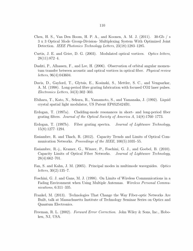
110

Chen, H. S., Van Den Boom, H. P. A., and Koonen, A. M. J. (2011). 30-Gb / s3 x 3 Optical Mode Group-Division- Multiplexing System With Optimized JointDetection. IEEE Photonics Technology Letters, 23(18):1283–1285.

Curtis, J. E. and Grier, D. G. (2003). Modulated optical vortices. Optics letters,28(11):872–4.

Dashti, P., Alhassen, F., and Lee, H. (2006). Observation of orbital angular momen-tum transfer between acoustic and optical vortices in optical fiber. Physical reviewletters, 96(4):043604.

Davis, D., Gaylord, T., Glytsis, E., Kosinski, S., Mettler, S. C., and Vengsarkar,A. M. (1998). Long-period fibre grating fabrication with focused CO2 laser pulses.Electronics Letters, 34(3):302–303.

Ebihara, T., Kato, N., Sekura, R., Yamamoto, S., and Yamanaka, J. (1992). Liquidcrystal spatial light modulator, US Patent EP0525424B1.

Erdogan, T. (1997a). Cladding-mode resonances in short- and long-period fibergrating filters. Journal of the Optical Society of America A, 14(8):1760–1773.

Erdogan, T. (1997b). Fiber grating spectra. Journal of Lightwave Technology,15(8):1277–1294.

Essiambre, R. and Tkach, R. (2012). Capacity Trends and Limits of Optical Com-munication Networks. Proceedings of the IEEE, 100(5):1035–55.

Essiambre, R.-j., Kramer, G., Winzer, P., Foschini, G. J., and Goebel, B. (2010).Capacity Limits of Optical Fiber Networks. Journal of Lightwave Technology,28(4):662–701.

Fan, S. and Kahn, J. M. (2005). Principal modes in multimode waveguides. Opticsletters, 30(2):135–7.

Foschini, G. J. and Gans, M. J. (1998). On Limits of Wireless Communications in aFading Environment when Using Multiple Antennas. Wireless Personal Commu-nications, 6:311–335.

Frankel, M. (2013). Technologies That Change the Way Fiber-optic Networks AreBuilt, talk at Massachusetts Institute of Technology Seminar Series on Optics andQuantum Electronics.

Freeman, R. L. (2002). Forward Error Correction. John Wiley & Sons, Inc., Hobo-ken, NJ, USA.

111

Freund, R., Bunge, C., Ledentsov, N., Molin, D., and Caspar, C. (2010). High-SpeedTransmission in Multimode Fibers. Journal of Lightwave Technology, 28(4):569–586.

Friberg, A. T. and Dandliker, R., editors (2008). Advances in Information Opticsand Photonics. SPIE Press.

Galtarossa, A., Palmieri, L., Pizzinat, A., Schiano, M., and Tambosso, T. (2000).Measurement of local beat length and differential group delay in installed single-mode fibers. Journal of Lightwave Technology, 18(10):1389–1394.

Garito, A. F., Wang, J., and Gao, R. (1998). Effects of Random Perturbations inPlastic Optical Fibers. Science, 281(5379):962–967.

Gibson, G., Courtial, J., Padgett, M., Vasnetsov, M., Pas’ko, V., Barnett, S., andFranke-Arnold, S. (2004). Free-space information transfer using light beams car-rying orbital angular momentum. Optics Express, 12(22):5448–56.

Gloge, D. (1972). Optical Power Flow in Multimode Fibers. The Bell SystemTechnical Journal, 51(8):1767–1783.

Gloge, D. and Marcatili, E. (1973). Multimode Theory of Graded-Core Fibers. TheBell System Technical Journal, 52(9):1563–1578.

Golowich, S., Bozinovic, N., Kristensen, P., and Ramachandran, S. (2013). Com-plex mode amplitude measurement for a six-mode optical fiber. Optics Express,21(4):4931–4944.

Golowich, S. and Ramachandran, S. (2005). Impact of fiber design on polarizationdependence in microbend gratings. Optics Express, 13(18):6870–7.

Gordon, J. P. and Kogelnik, H. (2000). PMD fundamentals: polarization modedispersion in optical fibers. Proceedings of the National Academy of Sciences ofthe United States of America, 97(9):4541–50.

Gregg, P., Kristensen, P., Golowich, S. E., Olsen, J. O., Steinvurzel, P., and Ra-machandran, S. (2013). Stable Transmission of 12 OAM States in Air-Core Fiber.to appear in CLEO:2013 - Laser Applications to Photonic Applications.

Groblacher, S., Jennewein, T., Vaziri, A., Weihs, G., and Zeilinger, A. (2006). Ex-perimental quantum cryptography with qutrits. New Journal of Physics, 8(5):75.

Hamming, R. (1950). Error detecting and error correcting codes. Bell Systemtechnical journal, XXIX(2):147–160.

112

He, H., Heckenberg, N. R., and Rubinsztein-Dunlop, H. (1995). Optical Parti-cle Trapping with Higher-order Doughnut Beams Produced Using High EfficiencyComputer Generated Holograms. Journal of Modern Optics, 42(1):217–223.

Hell, S. W. and Wichmann, J. (1994). Breaking the diffraction resolution limit bystimulated emission: stimulated-emission-depletion fluorescence microscopy. Op-tics Letters, 19(11):780–2.

Hill, K. O., Fujii, Y., Johnson, D. C., and Kawasaki, B. S. (1978). Photosensitivityin optical fiber waveguides: Application to reflection filter fabrication. AppliedPhysics Letters, 32(10):647–649.

Hill, K. O., Malo, B., Vinberg, K. A., Bilodeau, F., Johnson, D. C., and Skinner,I. (1990). Efficient mode conversion in telecommunication fibre using externallywritten gratings. Electronics letters, 26(16):1270–1272.

Ho, K.-P. and Kahn, J. M. (2011). Statistics of Group Delays in Multimode FiberWith Strong Mode Coupling. Journal of Lightwave Technology, 29(21):3119–3128.

Ho, K.-P. and Kahn, J. M. (2012). Delay-Spread Distribution for Multimode FiberWith Strong Mode Coupling. IEEE Photonics Technology Letters, 24(21):1906–1909.

Ho, K.-P. and Kahn, J. M. (2013). Mode Coupling and its Impact on SpatiallyMultiplexed Systems. In Kaminow, I. P., Li, T., and Willner, A. E., editors,Optical Fiber Telecommunications VI. Elsevier, Amsterdam.

Hwang, I. K., Yun, S. H., and Kim, B. Y. (1999). Long-period fiber gratings basedon periodic microbends. Optics Letters, 24(18):1263–1265.

Iizuka, K. (2002). Elements of Photonics Vol II. Wiley-Interscience.

Ip, E., Lau, A. P. T., Barros, D. J. F., and Kahn, J. M. (2008). Coherent detectionin optical fiber systems. Optics express, 16(2):753–91.

Jackson, J. (1962). Classical Electrodynamics. John Wiley & Sons., New York.

Jennewein, T., Simon, C., Weihs, G., Weinfurter, H., and Zeilinger, A. (2000). Quan-tum cryptography with entangled photons. Physical Review Letters, 84(20):4729–32.

Kao, K. and Hockham, G. (1966). Dielectric-fibre surface waveguides for opticalfrequencies. Electrical Engineers, Proceedings of IEE, 113(7):1151–1158.

Karimi, E., Marrucci, L., de Lisio, C., and Santamato, E. (2012). Time-divisionmultiplexing of the orbital angular momentum of light. Optics letters, 37(2):127–9.

113

Kashyap, R. (2008). Fiber Bragg Gratings. Academic Press, 2nd edition.

Khonina, S. N., Kotlyar, V. V., Shinkaryev, M. V., Soifer, V. A., and Uspleniev, G. V.(1992). The phase rotor filter. Journal of Modern Optics, 39(5):1147–1154.

Kogelnik, H. and Shank, C. V. (1972). Coupled-Wave Theory of Distributed Feed-back Lasers. Journal of Applied Physics, 43(5):2327–35.

Kreysing, M. K., Kieß ling, T., Fritsch, A., Guck, J. R., and Josef, A. K. (2008). Theoptical cell rotator. Optics Express, 16(21):912–914.

Ladavac, K. and Grier, D. (2004). Microoptomechanical pumps assembled and drivenby holographic optical vortex arrays. Optics Express, 12(6):1144–9.

Lee, B. G., Baks, C., Doany, F. E., Kuchta, D. M., Pepeljugoski, P., and Schow, C. L.(2012). Multicore Fiber Link Demonstrating Large Bandwidth Density for FutureMultimode Optical Interconnects. Proceedings of SPIE, Optoelectronic IntegratedCircuits XIV, 8265:826503.

Li, Y., Froggatt, M., and Erdogan, T. (2001). Volume current method for analysisof tilted fiber gratings. Journal of Lightwave Technology, 21(10):1580–1591.

Lines, M. E., Reed, W. A., Giovanni, D. J. D., and Hamblin, J. R. (1999). Ex-planation of anomalous loss in high delta singlemode fibres. Electronics Letters,35(12):1009–1010.

Mandel, L. and Wolf, E. (1995). Optical Coherence and Quantum Optics. CambridgeUniversity Press.

Marcuse, D. (1974). Theory of Dielectric Optical Waveguides. Academic Press.

Marcuse, D., Chraplyvy, A., and Tkach, R. (1991). Effect of fiber nonlinearity onlong-distance transmission. Journal of Lightwave Technology, 9(1):121–128.

Matsumoto, N., Ando, T., Inoue, T., Ohtake, Y., Fukuchi, N., and Hara, T. (2008).Generation of high-quality higher-order Laguerre-Gaussian beams using liquid-crystal-on-silicon spatial light modulators. Journal of the Optical Society of Amer-ica. A, Optics, image science, and vision, 25(7):1642–51.

McGloin, D., Simpson, N. B., and Padgett, M. J. (1998). Transfer of orbital angularmomentum from a stressed fiber-optic waveguide to a light beam. Applied optics,37(3):469–72.

Meltz, G., Morey, W. W., and Glenn, W. H. (1989). Formation of Bragg gratings inoptical fibers by a transverse holographic method. Optics letters, 14(15):823–5.

114

Meyer-Scott, E., Hubel, H., Fedrizzi, a., Erven, C., Weihs, G., and Jennewein, T.(2010). Quantum entanglement distribution with 810 nm photons through telecomfibers. Applied Physics Letters, 97(3):031117.

Milione, G., Sztul, H., Nolan, D., and Alfano, R. (2011). Higher-Order PoincareSphere, Stokes Parameters, and the Angular Momentum of Light. Physical ReviewLetters, 107(5):053601.

Mizrahi, V. and Sipe, J. (1993). Optical properties of photosensitive fiber phasegratings. Journal of Lightwave Technology, 11(10):1513–1517.

Noe, R., Sandel, D., Hinz, S., Mirvoda, V., Sch, A., Glingener, C., Gottwald, E.,Scheerer, C., Fischer, G., Weyrauch, T., Haase, W., Yoshida-Dierolf, M., Schopflin,A., and Gungener, C. (1999). Polarization Mode Dispersion Compensation at10, 20, and 40 Gb / s with Various Optical Equalizers. Journal of LightwaveTechnology, 17(9):1602–1616.

Olshansky, R. (1975). Mode Coupling Effects in Graded-index Optical Fibers. Ap-plied optics, 14(4):935–45.

Olshansky, R. and Nolan, D. A. (1976). Mode-dependent attenuation of opticalfibers: excess loss. Applied optics, 15(4):1045–1047.

Padgett, M., J, A., Simpson, N., and Allen, L. (1996). An experiment to observe theintensity and phase structure of LaguerreGaussian laser modes. American Journalof Physics, 64(1):77–82.

Padgett, M. J. and Courtial, J. (1999). Poincare-sphere equivalent for light beamscontaining orbital angular momentum. Optics letters, 24(7):430–2.

Panicker, R. A. and Kahn, J. M. (2009). Algorithms for Compensation of Multi-mode Fiber Dispersion Using Adaptive Optics. Journal of Lightwave Technology,27(24):5790–5799.

Patel, K. M. and Ralph, S. E. (2002). Enhanced Multimode Fiber Link Perfor-mance Using a Spatially Resolved Receiver. IEEE Photonics Technology Letters,14(3):393–395.

Pedersen, E. M., Kristensen, P., Gruner-nielsen, L., and Rottwitt, K. (2011). Impactof the Scalar Approximation on the Prediction of the Group Velocity Dispersion.Journal of Lightwave Technology, 29(21):3129–3134.

Pepeljugoski, P., Golowich, S. E., Ritger, A. J., Kolesar, P., and Risteski, A. (2003).Modeling and Simulation of Next-Generation Multimode Fiber Links. Journal ofLightwave Technology, 21(5):1242–1255.

115

Petrovich, M. N., Poletti, F., Wooler, J. P., Heidt, A. M., Baddela, N. K., Li, Z., Gray,D. R., Slavık, R., Parmigiani, F., Wheeler, N. V., Hayes, J. R., Numkam, E., Grner-Nielsen, L., Palsdottir, B., Phelan, R., Kelly, B., Becker, M., MacSuibhne, N., Zhao,J., Gunning, F. G., Ellis, A. D., Petropoulos, P., Alam, S. U., and Richardson, D. J.(2012). First Demonstration of 2um Data Transmission in a Low-Loss HollowCore Photonic Bandgap Fiber. In European Conference and Exhibition on OpticalCommunication, OSA Technical Digest (online), paper Th.3.A.5.

Poole, C. and Presby, H. (1995). Optical fiber spatial mode converter using periodiccore deformation, US Patent 5411566.

Poole, C. and Wagner, R. (1986). Phenomenological approach to polarisation dis-persion in long single-mode fibres. Electronics Letters, 22(19):1029–30.

Poole, C. D., Townsend, C. D., and Nelson, K. (1990). Resonant-helix two-modefiber notch filter. In Optical Fiber Communication Conference, OSA TechnicalDigest, paper TUG2. Optical Society of America.

Poppe, A., Fedrizzi, A., Ursin, R., Bohm, H., Lorunser, T., Maurhardt, O., Peev, M.,Suda, M., Kurtsiefer, C., Weinfurter, H., Jennewein, T., and Zeilinger, A. (2004).Practical quantum key distribution with polarization entangled photons. OpticsExpress, 12(16):3865–71.

Poynting, J. (1909). The wave motion of a revolving shaft, and a suggestion as tothe angular momentum in a beam of circularly polarised light. Proceedings of theRoyal Society of London, Series A(82):560–567.

Raddatz, L., White, I., Cunningham, D., and Nowell, M. (1998). An experimentaland theoretical study of the offset launch technique for the enhancement of thebandwidth of multimode fiber links. Journal of Lightwave Technology, 16(3):324–331.

Ramachandran, S. (2005). Dispersion-tailored few-mode fibers: a versatile platformfor in-fiber photonic devices. Journal of Lightwave Technology, 23(11):3426–3443.

Ramachandran, S., Fini, J., Mermelstein, M., Nicholson, J., Ghalmi, S., and Yan,M. (2008). Ultra-large effective-area, higher-order mode fibers: a new strategy forhigh-power lasers. Laser & Photonics Review, 2(6):429–448.

Ramachandran, S., Kristensen, P., and Yan, M. F. (2009). Generation and propaga-tion of radially polarized beams in optical fibers. Optics Letters, 34(16):2525–7.

Ramachandran, S., Nicholson, J., Ghalmi, S., and Yan, M. (2003). Measurement ofmultipath interference in the coherent crosstalk regime. IEEE Photonics Technol-ogy Letters, 15(8):1171–1173.

116

Randel, S., Ryf, R., Sierra, A., Winzer, P. J., Gnauck, A. H., Bolle, C. A., Peckham,D. W., Mccurdy, A., and Lingle, R. J. (2011). 6x56-Gb/s mode-division multi-plexed transmission over 33-km few-mode fiber enabled by 6x6 MIMO equalization.Optics Express, 19(17):16697–16707.

Richardson, D. J. (2010). Filling the Light Pipe. Science, 330(6002):327–328.

Rogers, A. (2008). Polarization in Optical Fibers. Artech House, Inc., Boston;London.

Ryf, R., Randel, S., Gnauck, A. H., Bolle, C., Sierra, A., Member, S., Mumtaz, S.,Esmaeelpour, M., Burrows, E. C., Essiambre, R.-j., Winzer, P. J., Peckham, D. W.,Mccurdy, A. H., and Lingle, R. (2012). Mode-Division Multiplexing Over 96 kmof Few-Mode Fiber Using Coherent 6x6 MIMO Processing. Journal of LightwaveTechnology, 30(4):521–531.

Sakaguchi, J., Awaji, Y., Wada, N., Kanno, A., Kawanishi, T., Hayashi, T., Taru,T., Kobayashi, T., and Watanabe, M. (2012). Space Division Multiplexed Trans-mission of 109-Tb/s Data Signals Using Homogeneous Seven-Core Fiber. Journalof Lightwave Technology, 30(4):658–665.

Saleh, B. and Teich, M. (2007). Fundamentals of Photonics. Wiley-Interscience,Hoboken, N.J., 2nd edition.

Salsi, M., Koebele, C., Sperti, D., Tran, P., Mardoyan, H., Brindel, P., Bigo, S.,Boutin, A., Verluise, F., Sillard, P., Bigot-astruc, M., Provost, L., and Charlet, G.(2012). Mode-Division Multiplexing of 2x100 Gb / s Channels Using an LCOS-Based Spatial Modulator. Journal of Lightwave Technology, 30(4):618–623.

Savin, S., Digonnet, M. J., Kino, G. S., and Shaw, H. J. (2000). Tunable mechanicallyinduced long-period fiber gratings. Optics letters, 25(10):710–2.

Schmitz, C. H. J., Uhrig, K., Spatz, J. P., and Curtis, J. E. (2006). Tuning the orbitalangular momentum in optical vortex beams. Optics express, 14(15):6604–12.

Shannon, C. (1948). A mathematical theory of communication. The Bell SystemTechnical Journal, 27(July, October):379–423, 623–656.

Shemirani, M. and Kahn, J. (2009). Higher-Order Modal Dispersion in Graded-IndexMultimode Fiber. Journal of Lightwave Technology, 27(23):5461–5468.

Shemirani, M. B., Mao, W., Panicker, R. A., and Kahn, J. M. (2009). PrincipalModes in Graded-Index Multimode Fiber in Presence of Spatial- and Polarization-Mode Coupling. Journal of Lightwave Technology, 27(10):1248–1261.

117

Sleiffer, V. A. J. M., Jung, Y., Veljanovski, V., Uden, R. G. H. V., Kuschnerov, M.,Inan, B., Nielsen, L. G., Sun, Y., Richardson, D. J., Alam, S. U., Poletti, F., Sahu,J. K., Dhar, A., Koonen, A. M. J., Corbett, B., Winfield, R., Ellis, A. D., andWaardt, H, D. (2012). 73.7 Tb/s (96x3x256-Gb/s) moe-division-multiplexed DP-16QAM transmission with inline MM-EDFA. Optics Express, 20(26):B428–B438.

Smink, R., de Hon, B., and Tijhuis, A. (2007). Bending loss in optical fibersa full-wave approach. Journal Of The Optical Society Of America B Optical Physics,24(10):2610–2618.

Smith, A. M. (1980). Birefringence induced by bends and twists in single-modeoptical fiber. Applied optics, 19(15):2606–11.

Snyder, A. and Love, J. (1983). Optical Waveguide Theory. Chapman and Hall,London; New York.

Stuart, H. R. (2000). Dispersive Multiplexing in Multimode Optical Fiber. Science,289(5477):281–283.

Su, T., Scott, R. P., Djordjevic, S. S., Fontaine, N. K., Geisler, D. J., Cai, X., and Yoo,S. J. B. (2012). Demonstration of free space coherent optical communication usingintegrated silicon photonic orbital angular momentum devices. Optics Express,20(9):9396–402.

Sullivan, M. N. O., Mirhosseini, M., Malik, M., and Boyd, R. W. (2012). Near-perfectsorting of orbital angular momentum and angular position states of light. OpticsExpress, 20(22):24444–24449.

Sunnerud, H., Xie, C., Karlsson, M., Samuelsson, R., and Andrekson, P. A. (2002).A Comparison Between Different PMD Compensation Techniques. Journal ofLightwave Technology, 20(3):368–378.

Tabosa, J. and Petrov, D. (1999). Optical Pumping of Orbital Angular Momentumof Light in Cold Cesium Atoms. Physical Review Letters, 83(24):4967–4970.

Takara, H., Sano, A., Kobayashi, T., Kubota, H., Kawakami, H., Matsuura, A.,Miyamoto, Y., Abe, Y., Ono, H., Shikama, K., Goto, Y., Tsujikawa, K., Sasaki,Y., Ishida, I., Takenaga, K., Matsuo, S., Saitoh, K., Koshiba, M., and Morioka, T.(2012). 1.01-Pb/s (12 SDM/222 WDM/456 Gb/s) Crosstalk-managed Transmis-sion with 91.4-b/s/Hz Aggregate Spectral Efficiency. In in European Conferenceand Exhibition on Optical Communication, OSA Technical Digest (online), paperTh.3.C.1.

Vengsarkar, A. M., Lemaire, P. J., Judkins, J. B., Bhatia, V., Erdogan, T., and Sipe,J. E. (1996). Long-Period Fiber Gratings as Band Rejection Filters. Journal ofLightwave Technology, 14(1):58–65.

118

Volpe, G. and Petrov, D. (2004). Generation of cylindrical vector beams with few-mode fibers excited by Laguerre-Gaussian beams. Optics Communications, 237(1-3):89–95.

Vuckovic, J. (2013). ”Optical Nanocavities with Quantum Dots: From Nano-lasersto Bio-probes” seminar, Massachusetts Institute of Technology Seminar Series onOptics and Quantum Electronics.

Wang, J., Yang, J.-y., Fazal, I. M., Ahmed, N., Yan, Y., Huang, H., Ren, Y., Yue,Y., Dolinar, S., Tur, M., and Willner, A. E. (2012). Terabit free-space data trans-mission employing orbital angular momentum multiplexing. Nature Photonics,6:488–496.

Wang, X., Nie, Q., Xu, T., and Liu, L. (2006). A Review of the Fabrication of OpticFiber. Proceedings of SPIE, International Commission for Optics ICO20: OpticalDesign and Fabrication, 6034:60341D.

Watson, G. (1995). A Treatise on the Theory of Bessel Functions. CambridgeUniversity Press, Cambridge.

Winzer, P. (2010). Beyond 100G Ethernet. IEEE Communications Magazine,48(July):26–30.

Winzer, P. and Essiambre, R. (2006). Advanced optical modulation formats. Pro-ceedings of the IEEE, 94(5):952–985.

Wong, G. K. L., Kang, M. S., Lee, H. W., Biancalana, F., Conti, C., Weiss, T., andRussell, P. S. J. (2012). Excitation of Orbital Angular Momentum Resonances inHelically Twisted Photonic Crystal Fiber. Science, 337(6093):446–449.

Yao, A. M. and Padgett, M. J. (2011). Orbital angular momentum: origins, behaviorand applications. Advances in Optics and Photonics, 3(2):161–204.

Yue, Y., Bozinovic, N., Ren, Y., Huang, H., Tur, M., Kristensen, P., Ramachandran,S., and Willner, A. E. (2013). 1.6-Tbit/s Muxing, Transmission and Demuxingthrough 1.1-km of Vortex Fiber Carrying 2 OAM Beams Each with 10 WavelengthChannels. In Optical Fiber Communication Conference/National Fiber Optic En-gineers Conference 2013, OSA Technical Digest (online), paper OTh4G.2.

CURRICULUM VITAE

Nenad Bozinovic

20 Chestnut St Apt 404, Cambridge, MA, 02139,+1-650-391-6600,

nesa@bu.edu, www.nenadbozinovic.com

EDUCATION

• May 2013 Ph.D. in Electrical and Computer Engineering, Boston University

• May 2007 M.Sc. in Electrical and Computer Engineering, Boston University,GPA: 3.61/4.0

• July 2004 B.Sc. in Physics, Belgrade University, Serbia, GPA: 9.6/10.0

AWARDS AND HONORS

• 2012 Top 20 downloaded paper of major optics journals (Advances in Opticsand Photonics, JOSA B and Optics Letters) over the past two years.

• 2011 Boston University President’s award for a top project among 100+graduate-level projects

• 2006 - 2010 Studenica Foundation Fellowship

• 1998 - 2004 Serbian Ministry of Education Fellowship

RESEARCH AND WORK EXPERIENCE

03/2010 - Present Research Assistant, Boston University, NanostructuredFibers and Nonlinear Optics Lab, Prof. Ramachandran Group

• Designed and developed system with potential for 400% throughput gain overexisting commercial fibers (collaboration with OFS Labs and USC)

• Developed modal characterization method for few-mode fibers (collaborationwith MIT Lincoln Laboratories)

• Demonstrated transmission of orbital angular momentum entangled photon pairover kilometer length fiber (collaboration with AT&T Labs)

120

05/2006 - 03/2010 Research Assistant, Boston University, BiomicroscopyLab

• Developed novel real-time, GPU-enabled, high-resolution microscopy techniquethat eliminates need for biopsies (prototype is currently used at Boston MedicalCenter)

05/2008 - 09/2008 Internship, Cambridge Research and InstrumentationInc. (now PerkinElmer)

• Identified new mouse brain imaging feature for DyCE Maestro, a company’sflagship product for cancer research, by improving core image processing algo-rithms.

SKILLS

• Fiber optics: Design, simulation, development and characterization of specialtyfibers and fiber devices

• Optics: Design and development of large (100+ components) opto-mechanical-imaging systems

• Imaging: CCD cameras, LCoS SLMs, MEMS, microscopy, image processing,visualization

• Optical Networks: Bit-error-rate testing; proficiency in optical components andmodulation formats

• Computer Networks: Ethernet, TCP/IP, HTTP protocols

• Programming: MATLAB, LabVIEW, C++/CUDA, COMSOL

• Hardware: LabVIEW automation: GPIB, USB, RS232 protocols

• Team-work: Coordinated research collaborations with MIT Lincoln Labs, AT&TLabs and USC

• Writing and presentation: Published 12 refereed papers; maximum presentationattendance 400+

121

PROFESSIONAL AND SOCIAL ACTIVITIES

• Reviewer for Optics Letters, Optics Express and IEEE Photonics TechnologyLetters journals

• Teaching assistant for ”Introduction to Semiconductor Physics” and ”Introduc-tion to Software Engineering”

• Boston University Waterpolo Team, 2008 and 2009

• Intramural sports: BU Tennis semi-finalist (2011); BU Soccer, Softball andFootball team member