Orbit Determination Using TDMA Radio Navigation

Data with Implicit Measurement Times

Ryan C. Dougherty∗ and Mark L. Psiaki†

Cornell University, Ithaca, New York, 14853-7501

An orbit determination Kalman filter has been developed that uses two types of mea-surements of time division multiple access (TDMA) L-Band signals from satellites in lowEarth orbit, a carrier phase measurement and a biased pseudorange measurement. Thisalgorithm will enable precise orbit determination of satellites broadcasting TDMA signalsnot originally intended for navigation. The TDMA structure of the carrier phase dataintroduces carrier phase ambiguities, which can be partially removed via preprocessingbased on rough orbit estimates. It is often impossible to remove a residual integer-valuedDoppler shift measured in cycles per data burst. The orbit determination square-rootinformation Kalman filter (SRIF) is a mixed real/integer extended Kalman filter whichdeals explicitly with the integer Doppler shift ambiguities of its partially corrected carrierphase measurements. It isolates the integer unknowns from the real-valued unknowns,and solves for its integer-valued estimates using an integer linear least-squares solver. Thecarrier phase and pseudorange measurements are available at known measurement timesat ground-based receivers, but they provide information about the satellite’s orbital stateat an unknown signal transmission time. An additional feature of the Kalman filter is itsexplicit treatment of the uncertain range delay. This is accomplished by applying a newtechnique that includes Chebyshev polynomial models of random process noise, dense out-put state interpolation that is consistent with numerical integration of the state differentialequation, iterative solution for signal transmission times, and consistent propagation of allof these effects through the SRIF. The effectiveness of this new Kalman filter has beenevaluated using truth-model data. The truth model simulation tests evaluate the filterresults against known “truth” states and known “truth” Doppler shift ambiguities. Thesimulation results predict that the Kalman filter will achieve RMS position errors of aboutXX meters magnitude using only five ground stations located in the contiguous UnitedStates.

I. Introduction

All manner of orbit determination problems are solved everyday, including post-processing, near real-timeorbit determination, and orbit predictions. A variety of algorithms are used to produce these estimates

of satellite position and velocity. Batch filtering and Kalman filtering are popular methods. Wheneverradio navigation data are used, the problem of dealing with implicit measurement times arises. This isnot a new problem, however the methods for dealing with the implicit measurement times are not alwaysmathematically rigorous. Recent work, however, has shown how to deal with implicit measurement timeswithin a Kalman filter.1

The signals used for orbit determination in this work are L-band TDMA down-link signals, never intendedfor use in orbit determination. When using TDMA signals, special considerations arise because the signalis not broadcast continuously. Between data bursts, some unknown integer number of carrier cycles elapses,and it is impossible to know exactly how many, because unmodeled accelerations and noise create Dopplershift uncertainty. Through clever preprocessing of the data based on rough orbit estimates, much of theresidual ambiguity can be removed, but there often remains some discrete set of possible residual Dopplershift errors. This Doppler shift error can be characterized by an integer number of carrier cycles per data

∗Graduate Student, Sibley School of Mechanical and Aerospace Engineering, AIAA Student Member†Professor, Sibley School of Mechanical and Aerospace Engineering, AIAA Associate Fellow

Copyright ©2011 by Ryan C. Dougherty andMark L. Psiaki. All rights reserved.

1 Preprint for the 2011 AIAA Guidance,Navigation, & Control Conference

AIAA Paper No. 2011-6493

burst. Figure 1 illustrates how the number of carrier cycles that elapse between data bursts can be uncertain.Note the two example possible carriers in the center of the figure that both connect the broadcast carriersat either end of the figure. They have different numbers of elapsed cycles. The preprocessing mentionedearlier cannot fully remove this uncertainty; instead it guarantees a certain correlation between the integeruncertainties of neighboring interburst periods.

Figure 1. Two successive data bursts (solid lines) and alternativepossible interburst carrier waves (dashed and dash-dotted lines).

This paper makes two main contribu-tions: one is to adapt the implicit mea-surement time Kalman filtering tech-niques of Ref. 1 to this orbit determi-nation problem, the other is to applythe techniques of Ref. 2 in order to di-rectly estimate the TDMA Doppler shiftambiguities as integers. The algorithmof Ref. 1 is applied in a straightfor-ward manner. It involves a generaliza-tion of the zero-order-hold process noiseassumption to polynomial process noiseand the solution of constraints that de-fine the measurement times. This is thefirst application of these techniques toorbit determination.

Estimation of the TDMA Dopplershift ambiguities gives rise to a mixedreal and integer estimation problem.This non-linear estimation problem islinearized using EKF-type methods, and the techniques of Ref. 2 are used to solve the resulting mixedreal and integer linear estimation problem.

Another contribution of this paper is its synthesis of the methods in Refs. 1 and 2 into a single algorithmthat can handle both implicit measurement times and Doppler shift integer ambiguities.

The remainder of this paper is organized into sections describing the various elements of the overall orbitdetermination algorithm. Section II defines the state vector and dynamics model used throughout. Section IIIdeals with the measurements and measurement model. It includes discussions of the measurement modelcomponents, the measurement constraint equation that implicitly determines the measurement effectivenesstime, and the linearization of the measurement equations. The filter is described in Section IV. It is asampled-data SRIF that is specially tailored to deal with implicit measurement times and mixed real andinteger estimation. Section V describes a truth model which was used to evaluate the efficacy of the filter.The paper ends with a short section that summarizes the results of truth model simulations and draws someconclusions.

II. Dynamics Modeling and Linearization

A. State Vector Definition

The state vector used in the present work is broken into four subsets of elements, x, bP , bφ, and n. The firstsubset represents the satellite state and parameters associated with the satellite. The second and third storethe real-valued carrier phase and pseudorange biases associated with each pass over each ground station.The fourth stores the integer-valued Doppler shift ambiguity associated with each pass over each groundstation.

The first subset, x, is composed of thirteen elements, as shown in Eq. (1).

x =[rT vT aT βd βs δt δf

]T(1)

The first six elements of x are the position vector, r, and velocity vector, v, of the spacecraft in Earth-centered inertially-fixed (ECIF) coordinates. The seventh through ninth elements, a, are the accelerationdisturbances in local level coordinates, each of which is modeled by a Markov process. The tenth and eleventhelements are the atmospheric drag inverse ballistic coefficient, βd, and the inverse solar radiation pressure

2

coefficient, βs; these are also modeled as Markov processes. The last two elements are spacecraft clock error,δt, and frequency error, δf , as in Ref. 3.

The second subset of state elements, bP , is a vector of real-valued pseudorange biases. The third subset,bφ, is a vector of real-valued carrier phase biases. Each time a ground station begins tracking a signal froma spacecraft, there is an associated unknown initial spacecraft clock time—the pseudorange bias—and anassociated constant, unknown, real-valued initial bias in the measured beat carrier phase. These biases arenuisance parameters and must be estimated along with the rest of the state.

The final subset of the state vector, n, is a vector of integer ambiguities, each associated with a particularground station and satellite pass. These constant integers count the number of carrier cycles that are over-or under-counted during the off-time of each TDMA signal per signal burst. They can be thought of asunknown integer Doppler shift biases.

B. Satellite State Dynamics

The time evolution of the x components of the state vector is modeled by a system of first-order, nonlinear,ordinary differential equations. The spacecraft trajectory is modeled by the summation of various componentsof a force model. All other spacecraft state elements are modeled as general Markov processes.

The differential equations that describe the satellite trajectory include the effects on the trajectory ofhigher-order Earth gravity terms, sun and moon gravity gradient, atmospheric drag, solar radiation pressure,and process noise. The Earth gravity model uses EGM96 coefficients in the non-singular recursion II ofTable 2 in Ref. 4. This model requires a coordinate transformation from the ECIF frame of r to the Earth-Centered Earth-fixed (ECEF) frame of the EGM96 model. This calculation is carried out using InternationalEarth Rotation and Reference System Service Bulletin B information. Sun and moon gravity gradients arecalculated using fully non-linear inverse square law gravity gradients and sun and moon locations calculatedusing the methods of Ref. 5, pp 70–73. Atmospheric drag is calculated using a cannon ball spacecraft modeland the Harris-Priester atmospheric density model.5 Solar radiation pressure is calculated using the inverseof the square of the actual distance from the sun to the satellite, which causes slight variations over thecourse of an orbit about the Earth. The calculation of solar radiation pressure also accounts for full andpartial occultation of the sun by the Earth.

The differential equations for this model take the form

r = v (2)

v = gESM (t, r) + ad(t, r,v, βd) + as(t, r, βs) +AECIF/LL(r,v)a (3)

where gESM is the gravitational acceleration due to the Earth, the sun, and the moon, ad is the accelerationdue to drag, as is the acceleration due to solar radiation pressure, AECIF/LL is the transformation from locallevel coordinates to ECIF coordinates, and a is the acceleration disturbance vector in local level coordinates.

The acceleration disturbances in local level coordinates are modeled as independent first-order GaussMarkov processes. They each have a time constant τa and a steady state acceleration standard deviationσa. They evolve according to the differential equation

a =−1

τaa + σa

√2

τawa (4)

where wa is white noise with E [wa(t)] = 0 and E[wa(t)wT

a (τ)]

= Iδ(t− τ).The drag inverse ballistic coefficient can be used to compute the acceleration due to drag by

ad(t, r,v, βd) = −1

2βdρ(r) ‖v − ωE × r‖ [v − ωE × r] (5)

where ρ(r) is the atmospheric density at the spacecraft position, ωE is the rotation rate of the Earth expressedin ECIF coordinates. The parameter βd itself is modeled by the following random walk differential equation

βd = wd (6)

where wd is white noise with E [wd] = 0 and E[wd(t)w

Td (τ)

]= qdδ(t − τ). If qd is set to zero, then βd is

modeled as a constant.

3

The solar radiation pressure coefficient can be used to model the solar radiation pressure accelerationwith

as(t, r) = −Ps0(rs, r)βs‖rs‖2

‖rs − r‖3[rs − r] (7)

where Ps0 is the nominal solar radiation pressure at 1 AU with a scaling to account for occultation of thesun by the Earth, and rs is the position of the sun. The parameter βs is also modeled by a random walk:

βs = ws (8)

where ws is white noise with E [ws] = 0 and E[ws(t)w

Ts (τ)

]= qsδ(t− τ). If qs is set to zero, then βs is

modeled as a constant.The last elements of the spacecraft state vector are the clock states. The clock is modeled with two

states—the spacecraft clock error and the oscillator frequency error. The oscillator frequency error is modeledas a random walk and the clock error is the integral of the oscillator frequency error plus another randomwalk. [

δt˙δf

]=

[0 1

0 0

][δt

δf

]+ wc (9)

As described in Ref. 3, the clock model process noise, wc, has statistics

E [wc(t)] = 0

E[wc(t)w

Tc (τ)

]= δ(t− τ)

[Sf 0

0 Sg

]where Sf and Sg are related to the Allan variance parameters by

Sf ∼ h0/2

Sg ∼ 2π2h−2

In summary, the satellite state vector model takes the form

x(t) = f (t,x(t),w(t)) (10)

where the 13 elements of the vector function f have been defined by Eqs. (2)–(4), Eq. (6), Eq. (8), and

Eq. (9). The noise vector w(t) =[wTa (t), wd(t), ws(t),w

Tc

]Thas seven elements described in the text

following Eq. (4), Eq. (6), Eq. (8), and Eq. (9).

C. Pseudorange Bias, Carrier Bias, and Doppler Ambiguity Dynamics

The individual elements of the pseudorange bias vector, bP , the carrier phase bias vector, bφ, and the Dopplershift ambiguity vector, n, are modeled as constants, but the number of elements of each vector can changeover time. In the case of the bP vector, with each new pass over each ground station, one new pseudorangebias is introduced. Thus, one includes the possibility of adding elements during the interval from sampletime tk to sample time tk+1

bPk+1 =

[bPk

δbPk+1

](11)

where bPk are the pseudorange biases that were introduced prior to tk and δbPk+1 are the new pseudorangebiases introduced between tk and tk+1, and the new pseudorange bias vector, bPk+1, at time tk+1 is theconcatenation of the bias vector at sample time tk and any new biases introduced on the interval betweentk and tk+1.

Like bPk, bφk must be allowed to grow to accommodate new carrier phase biases. Each new pass overeach ground station introduces a new bias, so define

bφk+1 =

[bφk

δbφk+1

](12)

4

where bφk+1, bφk, and δbφk+1 are defined analogously with the definitions of bPk+1, bPk, and δbPk+1, butthey apply to existing and new carrier phase biases.

The Doppler ambiguity vector, n, must be able to grow with time for the same reasons. So define

nk+1 =

[nk

δnk+1

](13)

where nk+1, nk, and δnk+1 are similarly defined, except that they apply to existing and new Doppler shiftambiguities rather than phase or pseudorange biases.

D. Satellite State Propagation

By numerically integrating Eq. (10) from time tk to time tk+1 > tk, given the satellite state at time tk anda continuous description of the process noise over that interval, the satellite state at time tk+1 can be found.Considering that the measurement signals are transmitted at some time before they are received, and thatthe transmission times will have to be solved through an implicit relationship, a continuous description ofthe satellite state over the interval from time tk to tk+1 must be kept. Such a description can take manyforms, but the one used herein is an appropriate interpolating polynomial for the Runge-Kutta numericalintegration algorithm. These interpolating polynomials are often called dense output Runge-Kutta methods.For more about dense output Runge-Kutta methods, see Refs. 5 and 6.

A continuous description of the process noise is also necessary. See Section II.F for more in-depthcoverage of this topic. For now, it suffices to say that the process noise over an integration interval isdescribed continuously by means of a polynomial. In the present work, Chebyshev polynomials describe theprocess noise over each integration interval. So, each element of the process noise vector over a given intervalis represented by the weighted sum of M + 1 Chebyshev polynomials of order 0 to M . The process noisemodel for integration interval k takes the form,

wk(t) =

M∑j=0

wjkCj (η(t, tk)) (14)

where Cj (η(t, tk)) is the jth order Chebyshev polynomial of the first kind, η(t, tk) = 2∆t (t − tk) − 1 is the

normalized time argument to the jth Chebyshev polynomial, ∆t is a constant defined as tk+1 − tk for allk, and wj

k is the vector of weighting coefficients for the process noise elements of the jth order polynomialvalid over the kth interval. As in Ref. 1 and described in Section II.F, the coefficients of the process noisepolynomials are modeled as a zero-mean white noise sequence such that the process noise is uncorrelatedfrom one interval to all others and optimally approximates the statistics of white noise. Also note that thecoefficients wj

k, though not known a priori, are estimated by the filter as parameters that affect the evolutionof the state over the interval.

In summary, the dynamic propagation computes the solution to the differential equation (10) using wk(t)as defined in Eq. (14) and starting at the initial condition x(tk) = xk. Formally, this solution can be writtenas

x(t; tk, tk+1,xk, w

0k, w

1k, . . . , w

Mk

)= x (t; Σk) , (15)

where Σk ,{tk, tk+1,xk, w

0k, w

1k, . . . , w

Mk

}.

This solution is available for all t in the interval tk to tk+1 through use of the Runge-Kutta interpolation.It is needed at measurement times that are to be determined and at the final time t = tk+1.

E. Linearized Satellite Dynamics

The filter described in Section IV is an extended Kalman filter which linearizes the dynamics and measure-ment model about estimates. The filter requires the partial derivatives of the state with respect to all of thevariables needed to propagate the state from time tk to tk+1. It also needs partial derivatives at intermediatetimes. The quantities needed are the state transition matrix,

Φk(t, tk) =∂x (t; Σk)

∂xk, (16)

5

and the influence matrices of the Chebyshev polynomial process noise coefficients,

Γjk(t, tk) =∂x (t; Σk)

∂wjk

for j = 0 to M. (17)

These are determined by Runge-Kutta integration and interpolation of their respective matrix initialvalue problems. See Ref. 1 for details.

It is convenient to lump the Chebyshev polynomial coefficient vectors into one large discrete-time processnoise vector.

wk =[

(w0k)T (w1

k)T . . . (wMk )T

]T(18)

and to define the corresponding influence matrix.

Γk(t, tk) =∂x (t; Σk)

∂wk=[

Γ0k(t, tk) Γ1

k(t, tk) . . . ΓMk (t, tk)]

(19)

These Jacobian matrices can be used to define linearized dynamics. First, it is helpful to define the pointabout which linearizations are being made. The process noise linearization point is the a priori process noiseestimate, wk = 0. The model requires a point for state linearization at all possible interpolation times inthe interval between sample times tk and tk+1. This point is

x(t; Σk) = x(t; tk, tk+1, xk, 0, . . . , 0) (20)

where xk is the a posteriori state estimate at sample time tk.The linearized dynamics now take the form[

x(t)− x(t; Σk)]

= Φk(t, tk)[xk − xk] + Γk(t, tk)wk (21)

One might be tempted to define ∆xk = x − xk, ∆x(t) = x(t) − x(t), and ∆xk+1 = ∆x(tk+1) and usethese quantities to simplify the above equation. This is not advisable because the definition of ∆xk+1 wouldchange in going from sample interval tk to tk+1 to sample interval tk+1 to tk+2.

Note the following shorthand notation is used to develop the Kalman filter: Φk = Φk(tk+1, tk), Γk =Γk(tk+1, tk), and xk+1 = x(tk+1; Σk). That is, when the time arguments are omitted, the state transitionmatrix and process noise influence matrix apply to the end of the time interval as does xk+1. These can beused to write the linearized filter dynamics model for the interval:

[xk+1 − xk+1] = Φk[xk − xk] + Γkwk (22)

This is just Eq. (21) evaluated at t = tk+1.

F. Chebyshev Polynomial Process Noise

This section briefly reviews the use of Chebyshev polynomials to approximate continuous-time white noiseand explains an appropriate statistical model. The material in this section paraphrases Section III.A. ofRef. 1. For additional information on the topics covered in this section, see that paper.

The motivation for using a polynomial description of process noise over an integration interval is a sideeffect of the numerical integration scheme used. The natural integration interval of the system is too longfor zero-order hold process noise to provide a good approximation of white noise over an entire integrationinterval. It is necessary to use a higher-order approximation of white noise that is consistent with useof implicit measurement times in a filter. Reference 1 shows how this can be done using the Chebyshevexpansion of Eq. (14).

In order to do this, it is necessary to define a statistical model for wk. The statistical model from Ref. 1is

E [wk] = 0. (23)

6

E[wk(wj)

T]

= δkj

α00Q 0 . . . 0

0 α11Q . . . 0...

.... . .

...

0 0 . . . αMMQ

(24)

where α00, α11, . . . , αMM are chosen to make the extension of the continuous time process noise modelin Eq. (14) to all integration intervals have an autocorrelation that is like the theoretical autocorrelation fortrue white noise:

E[w(t)wT(τ)

]= Qδ(t− τ) (25)

Specific coefficient values α00, α11, . . . , αMM are determined in Ref. 1 by solving an optimization problemthat maximizes the accuracy of this approximation. Several sets of optimal values are listed for several choicesof M in Ref. 1. Note that these coefficients set the covariance matrix of w and thus the a priori informationmatrix in what follows.

III. Measurement Modeling and Linearization

The following sections develop the model that relates the physical measurements used in this work to thestate of the system.

A. Measurement Model

The filter in the present work uses measurements of beat carrier phase and a biased pseudorange measure-ment. Beat carrier phase is the difference between the phase of the received signal and the phase of thereceiver’s replica of the nominal signal. Beat carrier phase can be measured very accurately, down to aboutone fortieth of a cycle. Pseudorange is the range-equivalent time difference between receiver clock time attime of reception and satellite clock time at time of transmission of designated signal features. The arrivaltime of a signal feature can be measured to within about one microsecond. The satellite clock time at timeof transmission of a particular feature is unknown, but the interval between features is regular and knownin satellite clock time.

1. Beat Carrier Phase Measurements

The following equation explicitly gives the range-equivalent beat carrier phase.

λφ = ρ+ c(τtropo − τiono − δt|tT ) + bφj + λ∆mni + vφ (26)

In this equation, λ is the wavelength of the carrier signal, φ is the beat carrier phase, c is the speedof light in vacuum, τtropo is the propagation delay due to the troposphere, τiono is the phase advance inseconds due to the ionosphere, δt|tT is the spacecraft clock error at transmission time, bφj is the carrierphase bias in meters associated with this measurement, ni is the Doppler shift ambiguity associated withthis measurement, ∆m is the number of data bursts that have elapsed since the initial data burst for thissignal was tracked, vφ is measurement noise, and ρ is the geometrical range between the satellite at time oftransmission and the ground station at time of reception, that is,

ρ =

√[rR|tR − r|tT ]

T[rR|tR − r|tT ] (27)

where rR|tR is the location of the receiver at the time of reception and r|tT is the location of the satellite atthe time of transmission.

The propagation delay due to refractivity of the neutral atmosphere, τtropo, is calculated using theSaastamoinen & Ifadis delay models.7 The ionosphere carrier phase advance τiono = 40.3·TEC

f2 is calculated

based on TEC from an ionospheric model. In this paper’s calculations, the Klobuchar model is used.8

The receiver clocks are assumed to be perfectly synchronized to true time. In the truth model simulation,this assumption is enforced. In actual fact, the receiver clock is not perfect, but it is disciplined to GPS time

7

using a coupled GPS receiver, and the errors in the receiver clock are much smaller than the errors in thesatellite clock.

A new carrier phase bias is added to the bφk vector every time a ground station begins tracking a signalfrom the satellite—once per pass overhead. In Eq. (26), bφj is the element of bφk+1 that applies to the carrierphase bias associated with the current pass of the reference station located at rR. The element bφj must beappended to the bias vector as part of δbφk in Eq. (12) for the time interval tk to tk+1 if and only if thefirst measurement sample of the given pass occurs in that time interval. The need for observability of thebφ vector precludes appending this bias element earlier.

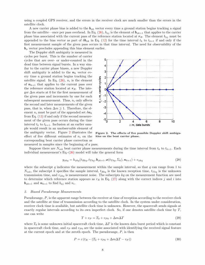
Figure 2. The effects of five possible Doppler shift ambigu-ities on the beat carrier phase.

The Doppler shift ambiguity is measured incycles per burst. This is the number of carriercycles that are over- or under-counted in thedead time between signal bursts. In a way sim-ilar to the carrier phase biases, a new Dopplershift ambiguity is added to the nk vector ev-ery time a ground station begins tracking thesatellite signal. In Eq. (26), ni is the elementof nk+1 that applies to the current pass overthe reference station located at rR. The inte-ger ∆m starts at 0 for the first measurement ofthe given pass and increments by one for eachsubsequent measurement. Thus, ni only affectsthe second and later measurements of the givenpass, that is, when ∆m ≥ 1. Therefore, the el-ement ni must be part of the appended set δnkfrom Eq. (13) if and only if the second measure-ment of the given pass occurs during the timeinterval tk to tk+1. Inclusion at an earlier sam-ple would result in an unobservable element ofthe ambiguity vector. Figure 2 illustrates theeffect of five different estimates of ni on thecorresponding beat carrier phase correction asmeasured in samples since the beginning of a pass.

Suppose there are Nmk beat carrier phase measurements during the time interval from tk to tk+1. Eachindividual measurement’s Eq.-(26) model will take the general form

yφkq = hφkq(tRkq, tTkq, bφk+1,x(tTkq,Σk),nk+1) + vφkq (28)

where the subscript q indicates the measurement within the sample interval, so that q can range from 1 toNmk, the subscript k specifies the sample interval, tRkq is the known reception time, tTkq is the unknowntransmission time, and vφkq is measurement noise. The subscripts kq on the measurement function are usedto determine which reference station appears as rR in Eq. (27) along with the correct indices j and i intobφk+1 and nk+1 to find bφj and ni.

2. Biased Pseudorange Measurements

Pseudorange, P , is the apparent range between the receiver at time of reception according to the receiver clockand the satellite at time of transmission according to the satellite clock. In the system under consideration,receiver clock time is available, but satellite clock time is unknown. However, the spacecraft sends signals atexactly regular intervals according to its own imperfect clock. So, if one denotes satellite clock time by T ,one can write

T + vP = T0 + vP0 + ∆m∆T (29)

where T0 is some unknown initial spacecraft clock time, ∆T is the known data burst period which is constantin spacecraft clock time, and vP and vP0 are the noise associated with identifying the received signal featureat the current epoch and at the zeroth epoch. The pseudorange, P , is then

P = c (tR − (T0 + vP0 + ∆m∆T − vP )) (30)

8

The apparent transit time can be broken into parts due to actual transit time and clock errors. Thegeometrical range, ρ, will contribute to the actual transit time. The signal will experience delays due topassing through the troposphere and ionosphere. These delays are the same as in Section III.A.1, exceptthat one uses τiono with the opposite sign, because the ionospheric phase advance is of equal magnitude andopposite sign as the ionospheric group delay. The apparent transit time is also affected by the receiver clockerror at time of reception and the satellite clock error at time of transmission. As stated earlier, the receiverclock error is assumed to be zero at all times, but the satellite clock will have some error, δt|tT , at the timeof signal transmission. The pseudorange can be written in terms of these apparent transit time componentsas

P = ρ+ c(τtropo + τiono − δt|tT ) (31)

Equating Eq. 30 with Eq. 31 and rearranging, we have

c (tR −∆m∆T ) = ρ+ c (τtropo + τiono + T0 + vP0 − δt|tT − vP ) (32)

The left-hand side of Eq. 32 contains only measured or known quantities. The right-hand side of Eq. 32contains quantities that depend on the filter states and quantities that can be calculated a priori, with theexception of the constant-over-one-pass quantity T0 + v0. This quantity is the initial spacecraft clock timewith associated measurement error, and it acts as a bias in the pseudorange measurements. Define

bP = T0 + v0 (33)

and the biased pseudorange measurement can be written explicitly as

c (tR −∆m∆T ) = ρ+ c (τtropo + τiono + bPl − δt|tT − vP ) (34)

As with carrier phase biases, a new pseudorange bias is added to the bias vector, bPk, at the beginning ofeach pass of the satellite over each ground station. In Eq. (34), bPl is the particular element of bPk associatedwith the current pass over the ground station at rR.

Also like the phase biases, the element bPl must be appended to the pseudorange bias vector as an elementof δbPk in Eq. (11) if and only if the first measurement sample of the current pass occurs in the intervalbetween tk and tk+1.

The general form of the biased pseudorange measurement equation will take a form analogous to Eq. (28).Each biased pseudorange measurement on the interval from tk to tk+1 will have an Eq.-(34) model of theform

yPkq = hPkq(tRkq, tTkq, bPk+1,x(tTkq,Σk)) + vPkq (35)

where all symbols are defined as before, and the subscripts kq perform a similar task to the same subscriptsin Eq. (28), they choose which reference station appears as rR in Eq. (27) and the correct index l into bPk+1

to find bPl.The physical measurements of the system are related to the satellite state at the time of signal transmission

through Eq. (28) and Eq. (35), but the time of signal transmission is still unknown.

B. Measurement Constraint

The unknown transmission time in the measurement model of Eq. (28) and Eq. (35) is determined from theknown reception time tR and the transmission delay. The transmission delay relationship can be written inthe form of the following constraint.

0 = c[tR − tT ]−√

[rR|tR − r|tT ]T

[rR|tR − r|tT ]− c(τiono + τtropo) (36)

where τiono, again represents the ionospheric group delay. The time of transmission, tT , is computed via anumerical solution of this equation. This numerical solution relies on knowing the function r(t) at varioustimes. This knowledge is provided by the Runge-Kutta state interpolation x(t; Σk).

For each of the Nmk beat carrier phase measurements and Nmk biased pseudorange measurements, therewill be a corresponding constraint equation that will take the general form

0 = gkq(tRkq, tTkq,x(tTkq,Σk)) (37)

where the subscripts kq on g perform analogous tasks as before; that is, they choose the correct groundstation to appear as rR in Eq. (36). Note the solution of this constraint for tTkq makes tTkq an implicitfunction of the elements of Σk, e.g., xk and wk.

9

C. Linearized Measurement Equations

The filter developed in Section IV requires a linearized measurement model. In order to develop thelinearized measurement model, derivatives of hφkq(tRkq, tTkq, bφk+1,x(tTkq,Σk),nk+1) and derivatives ofhPkq(tRkq, tTkq, bPk+1,x(tTkq,Σk)) must be computed. In particular, derivatives with respect to the vectorsbφk+1, bPk+1, nk+1, xk, and wk are necessary.

In naming the partial derivatives in Eq. (38)–Eq. (42), the first subscript indicates which measurementfunction is being differentiated—φ for carrier phase and P for pseudorange—the second subscript indicateswith respect to which quantity it is being differentiated, and the third and fourth subscripts indicate thetime step and sample number. When differentiating with respect to biases, the bias-type subscript has beenomitted; it is to be understood that differentiation is carried out with respect to the corresponding type ofbias. The partial derivatives of the carrier phase measurement function with respect to bφk+1 and nk+1 arestraightforward to write for the qth measurement on sample interval tk to tk+1.

Hφbkq =∂hφkq(tRkq, tTkq, bφk+1,x(tTkq,Σk),nk+1)

∂bφk+1(38)

Hφnkq =∂hφkq(tRkq, tTkq, bφk+1,x(tTkq,Σk),nk+1)

∂nk+1(39)

Likewise, the partial derivative of the pseudorange measurement function with respect to bPk+1 for the qth

pseudorange measurement on the same interval is also easy to find.

HPbkq =∂hPkq(tRkq, tTkq, bPk+1,x(tTkq,Σk))

∂bPk+1(40)

These three derivatives can be found by analytically differentiating the respective measurement functions.The derivatives of the measurement function with respect to xk and wk must be computed using the

chain rule of differentiation, because the functions

hφkq(tRkq, tTkq, bφk+1,x(tTkq,Σk),nk+1)

andhPkq(tRkq, tTkq, bPk+1,x(tTkq,Σk))

depend only indirectly upon xk and wk through x(tTkq,Σk) and through tTkq. The derivatives of the carrierphase measurement function with respect to xk and wk for the qth measurement on sample interval tk totk+1 are written1

Hφxkq =∂hφkq(tRkq, tTkq, bφk+1,x(tTkq; Σk),nk+1)

∂x(tTkq; Σk)

[∂x(tTkq; Σk)

∂xk+∂x(tTkq; Σk)

∂tTkq

∂tTkq∂xk

]+∂hφkq(tRkq, tTkq, bφk+1,x(tTkq; Σk),nk+1)

∂tTkq

∂tTkq∂xk

(41)

Hφwkq =∂hφkq(tRkq, tTkq, bφk+1,x(tTkq; Σk),nk+1)

∂x(tTkq; Σk)

[∂x(tTkq; Σk)

∂wk+∂x(tTkq; Σk)

∂tTkq

∂tTkq∂wk

]+∂hφkq(tRkq, tTkq, bφk+1,x(tTkq; Σk),nk+1)

∂tTkq

∂tTkq∂wk

(42)

In both Eq. (41) and Eq. (42) above, the hφkq partial derivative in each of the two main terms on theright-hand side can be found by taking the analytical derivative of the measurement function. The leftmostpartial derivatives inside the square braces in both equations are derivatives already defined in Eq. (16) andEq. (19). The first partial derivative in the second term of the expression in square braces in each equation isthe time derivative of the state. This quantity can, in general, be obtained in two ways: either by evaluatingEq. (10) with the proper arguments, or by differentiating the interpolating polynomial that is the output ofthe dense-output Runge-Kutta numerical integration. The former method is used in the present work.

10

The partial derivatives of tTkq with respect to xk and wk remain to be determined. The former appearsin two places in Eq. (41), the latter in two places in Eq. (42). These are determined via partial differentiationof the constraint that implicitly defines tTkq, the constraint in Eq. (37). The derivative with respect to xkis determined by solving the following differentiated form of that constraint.

0 =∂gkq (tRkq, tTkq,x(tTkq,Σk))

∂x(tTkq; Σk)

[∂x(tTkq; Σk)

∂xk+∂x(tTkq; Σk)

∂tTkq

∂tTkq∂xk

]+∂gkq (tRkq, tTkq,x(tTkq,Σk))

∂tTkq

∂tTkq∂xk

(43)

Notice that the unknown term ∂tTkq/∂xk enters linearly and that all other terms are either knownalready or can be found by taking analytical derivatives of the constraint equation. The solution of Eq. (43)can be substituted into Eq. (41) to complete the definition of Hφxkq. A similar procedure is used to compute∂tTkq/∂wk for substitution into Eq. (42). The resulting differentiated constraint varies from Eq. (43) in thatall partial derivatives with respect to xk change to partials with respect to wk. See Ref. 1 for the originalderivation of this method and for more details.

The derivatives HPxkq and HPwkq are found using the same procedure on hPkq(...) and the same differ-entiated constraint equation.

With the above derivatives, one can write the linearized measurement equation for the qth measurement onthe time interval tk to tk+1. Before proceeding, it is useful to define the points about which the measurementequation is linearized. The measurement equation is linearized about the a priori process noise estimate¯wk = 0, about the a priori pseudorange bias estimate

bPk+1 =

[bPk

0

](44)

about the a priori beat carrier phase bias estimate

bφk+1 =

[bφk

0

](45)

about the a priori Doppler shift ambiguity estimate

nk+1 =

[nk

0

](46)

and about the same satellite state point about which the dynamics are linearized, xk. The circumflexes(ˆ) indicate the a posteriori estimates at sample k, and the macrons (¯) indicate the a priori estimates atsample k+ 1. Now, the linearized carrier phase measurement equation for the qth measurement on the timeinterval tk to tk+1 is

[yφkq − hφkq(tRkq, tTkq, bφk+1, x(tTkq; Σk),nk+1)] = Hφwkqwk +Hφbφkq[bφk+1 − bφk+1]

+Hφxkq[xk − xk] +Hφnkq[nk+1 − nk+1] + vφkq (47)

and the linearized pseudorange measurement equation for the qth pseudorange measurement on the sameinterval is

[yPkq − hPkq(tRkq, tTkq, bPk+1, x(tTkq; Σk))] = HPwkqwk +HPbP kq[bPk+1 − bPk+1]

+HPxkq[xk − xk] + vPkq (48)

With one additional definition, all 2Nmk measurements in sample interval tk to tk+1 can be stacked intoa single matrix-vector equation. Let ∆y2kq , y2kq − h2kq(...), where 2 is either P or φ. Now all 2Nmk

11

equations can be stacked.

∆yφk1

∆yφk2

...

∆yφkNmk∆yPk1

∆yPk2

...

∆yPkNmk

=

Hφwk1 0 Hφbk1 Hφxk1 Hφnk1

Hφwk2 0 Hφbk2 Hφxk2 Hφnk2

......

......

...

HφwkNmk 0 HφbkNmk HφxkNmk HφnkNmk

HPwk1 HPbk1 0 HPxk1 0

HPwk2 HPbk2 0 HPxk2 0...

......

......

HPwkNmk HPbkNmk 0 HPxkNmk 0

wk

bPk+1 − bPk+1

bφk+1 − bφk+1

xk − xk

nk+1 − nk+1

+

vφk1

vφk2

...

vφkNmkvPk1

vPk2

...

vPkNmk

(49)

Finally, by combining each column in the above equation into a single vector or matrix, one arrives atthe final form of the linearized measurement vector equation.

∆yk+1 =[Hwk HPk+1 Hφk+1 Hxk Hnk+1

]

wk

bPk+1 − bPk+1

bφk+1 − bφk+1

xk − xk

nk+1 − nk+1

+ vk (50)

The row vectors that comprise the large block matrix in Eq. (49) are distinguished notationally from thematrices Hwk, HPk+1, Hφk+1, Hxk, and Hnk+1 in Eq. (50) only by two notational details. First, the formerretain the sample number subscript, while the latter do not. And, second, the former carry a leading φ orP subscript and, if applicable, a b subscript, while the latter have dropped their leading φ or P subscript,except in the second and third block columns of Eq. (50), in which the φ and P subscripts were kept infavor of the b subscript. Of course, the former are the rows of their respective counterparts in the latter.The sample indices have been incremented by one when stacking the row vectors HPbkq, Hφbkq, and Hφnkq

into the matrices HPk+1, Hφk+1, and Hnk+1. This was done to improve consistency in Eq. (50) and in whatfollows. Finally, with the linearized dynamics equation, Eq. (22), and the linearized measurement equation,Eq. (50), one can derive the square-root information extended Kalman filter.

IV. Square-Root Information Extended Kalman Filter

A. Square-Root Information Formulation

A square-root information equation stores estimates of the real- and integer-valued states, along with theirassociated uncertainties. The a posteriori square-root information equations used by the present filter are

RPPk RPφk RPxk RPnk

0 Rφφk Rφxk Rφnk

0 0 Rxxk Rxnk

0 0 0 Rnnk

bPk − bPk

bφk − bφk

xk − xk

nk − nk

=

0

0

0

∆znk

−vPk

vφk

vxk

vnk

(51)

The a posteriori information is stored in the square-root information matrices which comprise the largeblock matrix on the left-hand side of Eq. (51), in the a posteriori estimates, bPk, bφk, xk, and nk, and inthe information vector ∆znk. The block, upper-triangular, square-root information matrix on the left-handside is the inverse square-root of the a posteriori covariance matrix of the vector that multiplies it. Thewhite noise vectors, vPk, vφk, vxk, and vnk are independent, zero-mean, identity-covariance white noisesequences. Notice that only the last of the four equations has a non-homogeneous term, ∆znk, on theright-hand side. This is because the real-valued a posteriori estimates, bPk, bφk, and xk, have been chosento make their corresponding information equations homogeneous. The optimal estimate nk is chosen tominimize ∆zT

nk∆znk, but it cannot drive this cost metric to zero because it is restricted to take on integer

values. Note, a traditional SRIF, as in Ref. 9, does not have the bPk, bφk, xk, and nk terms that appear in

12

Eq. (51). Instead, all three equations have non-homogeneous terms. The nonstandard form of Eq. (51) isuseful in the context of extended SRIF for nonlinear problems.

The presence of process noise in Eq. (50) makes it more computationally efficient for the SRIF to performa combined dynamic propagation and measurement update than to perform each separately. The first stepforms a set of equations that combines an a priori process noise equation with the a posteriori informationequations, Eq. (51), and the measurement equations, Eq. (50), in that order.

Rwwk [0, 0] [0, 0] 0 [0, 0]

0 [RPPk, 0] [RPφk, 0] RPxk [RPnk, 0]

0 [0, 0] [Rφφk, 0] Rφxk [Rφnk, 0]

0 [0, 0] [0, 0] Rxxk [Rxnk, 0]

0 [0, 0] [0, 0] 0 [Rnnk, 0]

Hwk HPk+1 Hφk+1 Hxk Hnk+1

wk

bPk+1 − bPk+1

bφk+1 − bφk+1

xk − xk

nk+1 − nk+1

=

0

0

0

0

∆znk

∆yk+1

−

vwk

vPk

vφk

vxk

vnk

vk

(52)

where Rwwk is the process noise square-root information matrix, which is the inverse square root of thecovariance matrix given in Eq. (24). In combining Eq. (50) and Eq. (51), Eq. (51) has been re-written interms of bPk+1, bφk+1, and nk+1. This was accomplished by noting that bPk+1, bφk+1, and nk+1 equal,respectively, bPk, bφk, and nk, but possibly with additional elements as in Eq. (11), Eq. (12), and Eq. (13).The filter has no a priori information about the added elements, which is accounted for with the additionalcolumns of zeros in the second, third, and fifth block columns of the block matrix on the left-hand side ofEq. (52).

The second step in performing the combined propagation and update is to write the above equation interms of xk+1 − xk+1. If the linearized dynamics equation, Eq. (22), is solved for [xk − xk] in terms ofxk+1− xk+1 and wk, the first and fourth columns of the large block matrix change so that Eq. (52) becomes

Rwwk [0, 0] [0, 0] 0 [0, 0]

−RPxkΦ−1k Γk [RPPk, 0] [RPφk, 0] RPxkΦ−1

k [RPnk, 0]

−RφxkΦ−1k Γk [0, 0] [Rφφk, 0] RφxkΦ−1

k [Rφnk, 0]

−RxxkΦ−1k Γk [0, 0] [0, 0] RxxkΦ−1

k [Rxnk, 0]

0 [0, 0] [0, 0] 0 [Rnnk, 0]

Hwk−HxkΦ−1k Γk HPk+1 Hφk+1 HxkΦ−1

k Hnk+1

wk

bPk+1 − bPk+1

bφk+1 − bφk+1

xk+1 − xk+1

nk+1 − nk+1

=

0

0

0

0

∆znk

∆yk+1

−

vwk

vPk

vφk

vxk

vnk

vk

(53)

The remaining operations of the measurement update and dynamic propagation are accomplished byperforming orthogonal/upper triangular (QR) factorization10 of the large block matrix into an orthonormalmatrix T and an upper triangular matrix. One then multiplies both sides of Eq. (53) by TT. The large blockmatrix is made upper triangular and the following square-root information equations emerge.

Rwwk RwPk+1 Rwφk+1 Rwxk+1 Rwnk+1

0 RPPk+1 RPφk+1 RPxk+1 RPnk+1

0 0 Rφφk+1 Rφxk+1 Rφnk+1

0 0 0 Rxxk+1 Rxnk+1

0 0 0 0 Rnnk+1

0 0 0 0 0

wk

∆bPk+1

∆bφk+1

∆xk+1

∆nk+1

=

∆zwk

∆zPk+1

∆zφk+1

∆zxk+1

∆znk+1

∆zres

−

vwk+1

vPk+1

vφk+1

vxk+1

vnk+1

vres

, (54)

where the matrices along the diagonal of the large block matrix are all square, upper-triangular matrices ofappropriate dimension, and the matrices above the diagonal of the large block matrix are fully populated andappropriately dimensioned. In Eq. (54), the quantities in the vector that multiplies the large block matrix onthe left-hand side have been renamed for brevity to be ∆bPk+1 = bPk+1− bPk+1, ∆bφk+1 = bφk+1− bφk+1,∆xk+1 = xk+1 − xk+1, and ∆nk+1 = nk+1 − nk+1. The nonhomogeneous vector on the right-hand side ofEq. (54), the one involving ∆zwk, ∆zPk+1, etc., equals the nonhomogeneous vector from Eq. (53), the oneinvolving ∆znk and ∆yk+1, left-multiplied by TT. The residual error vector, ∆zres, is the SRIF equivalent ofa Kalman filter innovation. The noise vector has been transformed in the same way. It remains a zero-mean,identity-covariance white noise vector.

13

With the equations in this form, one can compute the optimal estimate of the integer vector ∆nk+1 beforecomputing the estimates of the real-valued vectors ∆bPk+1, ∆bφk+1, and ∆xk+1. The optimal estimate of∆nk+1 is found by solving the following integer linear least squares (ILLS) problem.

find: ∆nk+1

to minimize: J = 12

[Rnnk+1∆nk+1 −∆znk+1

]T [Rnnk+1∆nk+1 −∆znk+1

]subject to: ∆nk+1is an integer-valued vector

(55)

For details on how to solve such ILLS problems, see Refs. 11 and 12. Let ∆nk+1 be the value of ∆nk+1

that minimizes Eq. (55). The next step is to compute ∆znk+1 based on ∆znk+1 and ∆nk+1. The quantity∆znk+1 will be used in the next recursion of the filter, when k is incremented by one.

∆znk+1 = ∆znk+1 − Rnnk+1∆nk+1 (56)

The optimal a posteriori estimates of ∆bPk+1, ∆bφk+1, and ∆xk+1 are found by back substitution.

∆xk+1 = R−1xxk+1

[∆zxk+1 − Rxnk+1∆nk+1

](57)

∆bφk+1 = R−1φφk+1

[∆zφk+1 − Rφxk+1∆xk+1 − Rφnk+1∆nk+1

](58)

∆bPk+1 = R−1PPk+1

[∆zPk+1 − RPφk+1∆bφk+1 − RPxk+1∆xk+1 − RPnk+1∆nk+1

](59)

The a posteriori estimates of bPk+1, bφk+1, xk+1, and nk+1 can be computed by adding the a posterioriestimates of the perturbation to the a priori estimates.

bPk+1 = bPk+1 + ∆bPk+1 (60)

bφk+1 = bφk+1 + ∆bφk+1 (61)

xk+1 = xk+1 + ∆xk+1 (62)

nk+1 = nk+1 + ∆nk+1 (63)

At this point, filtering over the time step from tk to tk+1 is complete, and the a posteriori quantities maybe passed forward to initialize the next recursion of the filter. Section IV.C lists those matrices and vectorsthat must be passed forward from one time step to the next and gives a synopsis of the algorithm.

B. Deletion of Inactive Pseudorange and Carrier Phase Biases and Doppler Shift Ambiguities

Over time, as the spacecraft accumulates passes over the various ground stations, the dimensions of the bPand bφ vectors grow. At the completion of a pass over a ground station, the biases associated with that passwill no longer enter any measurement equations and will have no further effect on the state estimate. It isefficient to drop those elements out of bP and bφ in order to limit their size. Consider the combined vectorof biases b = [bT

P bTφ ]T at time tk+1, when there are Nb biases in the vector,

bk+1 =[b1 b2 . . . bi . . . bNb

]T(64)

Note that in the remainder of this section, the two bias vectors bP and bφ are concatenated together to forma single, simpler-to-write bias vector b. The notation for all other quantities has been adjusted accordinglyby forming larger block matrices or concatenations of vectors.

Suppose that the ground-station pass associated with bias bi in b is complete. Therefore, bi will nolonger appear in any measurement equations, and it can be discarded. This can be accomplished in three

14

steps. First, one permutes the elements of the composite vector on the left-hand side of Eq. 54 such thatthe element associated with bi is the first element of the composite vector,[

∆bi wTk ∆bT

k+1 ∆xTk+1 ∆nT

k+1

]T(65)

where ∆bk+1 is ∆bk+1 with ∆bi excised. This permutation necessitates a corresponding permutationof the columns of Rbbk+1 and Rwbk+1 in the left-hand side of Eq. (54), which permutation destroys theupper-triangularity of the block matrix.

Second, in order to restore the upper-triangularity of the permuted large block matrix, a new QR factor-ization must be applied to Eq. (54). The resulting equation is

Rbibi Rbiwk Rbibk+1 Rbixk+1 Rbink+1

0 Rwwk Rwbk+1 Rwxk+1 Rwnk+1

0 0 Rbbk+1 Rbxk+1 Rbnk+1

0 0 0 Rxxk+1 Rxnk+1

0 0 0 0 Rnnk+1

0 0 0 0 0

∆bi

wk

∆bk+1

∆xk+1

∆nk+1

=

∆zbi∆zwk

∆zbk+1

∆zxk+1

∆znk+1

∆zres

−

vbivwk+1

vbk+1

vxk+1

vnk+1

vres

(66)

Third and finally, the first row of Eq. (66) is dropped from the problem along with the left-most columnof the large block matrix on the left-hand side of Eq (66).

One might be tempted to drop integer-valued Doppler shift ambiguities in an analogous manner, if theytoo apply to completed ground-station passes. In fact, this produces a suboptimal solution. If the giveninteger element of n is known with a very high degree of certainty when it is dropped, then optimalitycan be maintained, but with a modified dropping procedure.2 In general, it is difficult to be certain thatthe estimated integers are exactly correct. By carrying the integers forward forever, the optimal solution isfound. A problem with this approach, however, is that the integer vector grows in length. The resulting ILLSproblem can become very costly to solve after each measurement update. A reasonable suboptimal solutionis found by dropping an integer-valued state after a significant interval has elapsed since it last entered ameasurement equation. The optimal and suboptimal integer dropping methods are treated in more detail inRef. 2. In the present work, the integers are dropped as if they were real-valued after a reasonable time haselapsed since they last entered a measurement equation.

C. Algorithm

The following steps summarize the algorithm presented in this paper.

1. Set k = 0

2. Numerically integrate from tk to tk+1 to find xk+1, Φk, and Γk.

3. Set up Eq. (53) with the known quantities from the previous time step, or with the initial estimatesif k = 0, and append the measurements accumulated between time tk and time tk+1. The quantitiescarried forward from the last time step are RPPk, RPφk, RPxk, RPnk, Rφφk, Rφxk, Rφnk, Rxxk, Rxnk,

Rnnk, ∆znk, and the a posteriori bias, state, and ambiguity estimates from the previous time step.

4. QR factorize and transform to get Eq. (54).

5. Drop biases that will no longer appear in any measurement equations, as per Section IV.B.

6. If dropping integers, drop those which last appeared in a measurement equation more than Ns timesteps ago, where Ns is some threshold value, as per Ref. 2.

7. Solve the ILLS problem for ∆nk+1.

8. Solve for ∆znk+1, ∆xk+1, ∆bφk+1, and ∆bPk+1 using Eqs. (56)–(59).

9. Solve for the estimates bPk+1, bφk+1, xk+1, and nk+1 using Eqs. (60)–(63)

10. Set k = k + 1, and go to Step 2.

15

V. Truth Model Simulation

In order to evaluate the effectiveness of the filter, it was applied to data that were derived from a truthmodel simulation. The truth model simulation generates truth values for the process noise polynomialcoefficients, and uses them to generate the truth state vector time history. The simulation synthesizesmeasurements by using the true state history in the measurement equation, and by adding in the effects ofphase bias, pseudorange bias, Doppler shift ambiguity, and measurement noise. The filter is then able tooperate on these synthesized measurements, and the results can be compared to the true values from thesimulation.

The values of the process noise polynomial coefficients were generated using a pseudo-random numbergenerator to draw samples from normal distributions with statistics as described in Section II.F. In thesimulation, fourth-order Chebyshev polynomials were used to approximate process noise. The optimal valuesof the “α” coefficients of Eq. (24) for fourth-order process noise are taken from Ref. 1. Once the processnoise polynomial coefficients for an interval are chosen, the process noise affecting the system can be foundat any point on the interval by evaluating the weighted sum of polynomials, Eq.( 14).

Given realistic initial conditions for a LEO satellite and the process noise polynomial coefficients for allintegration intervals, the truth model simulation numerically integrates the dynamics equations forward intime in order to generate the truth orbit. The truth model simulation uses the same dynamics equations asthe filter.

The truth model simulation starts with the reception times of the measurements at all ground stationsas givens, and it uses the constraint equation and the state interpolation from the dense-output numericalintegration to calculate the time of transmission from the satellite and the location of the satellite at thattime. From this information, the time history of received beat carrier phase is generated. The pseudorangebias is generated by adding white, Gaussian, zero-mean noise with standard deviation of 1 microsecond tothe arrival times. A random, constant offset added to the phase history for each pass over each groundstation accounts for the effects of phase bias. The Doppler shift integer ambiguity, ni, is generated bysampling the set {−3,−2,−1, 0, 1, 2, 3} with equal probability and using this value as the number of cyclesthat ramps linearly with measurement number, as per Eq. (26). The random component of the carrierphase measurement error, v in Eq. (26), is sampled from a zero-mean Gaussian distribution with standarddeviation of 4.6 mm.

Figure 3. The approximate locations of the five simulated groundstations.

The truth model simulation usedfor the purposes of this paper includedfive simulated ground stations locatedin the continental United States. Fig-ure 3 shows the locations of the fiveground stations. The orbits used inthe truth model simulation were nearly-circular, nearly-polar orbits with periodof about 100 minutes. Each ground sta-tion recorded measurements at a rateof 1.1 Hz when the satellite was above10 degrees elevation with respect to theground station. The satellite’s clockmodel parameters were chosen to giveit characteristics approximating those ofan ovenized crystal oscillator: h0 =2E−22 s and h−2 = 6.1E−22 1/s, whichgives a minimum root Allen variance of3.56E-11 at a time delay of 0.158 s.

The truth model simulation testsprovided a means to evaluate filter performance under controlled conditions with known truth states. Theavailability of truth states made it easy to investigate filter convergence by perturbing the initial state es-timate around the true initial state. Using the truth states, it was also possible to carry out statisticalconsistency checks of the filter that would otherwise have been impossible to perform. The truth model alsoprovided a means of quickly evaluating filter performance under ideal conditions.

16

VI. Results

Several simulations were run, all with the same initial conditions, but each with new, randomly selectedprocess noise. Filter convergence was investigated using some of the shorter simulations by running thefilter several times with different initial estimation errors and covariances. For each of the filter runs, filterconsistency and performance were checked. Filter performance results given below are averaged over fiveindependent 25-hour filter runs. This duration yields three distinct sets of passes over the continental UnitedStates. Also discussed in detail are results from a single, characteristic 25-hour run. No attempt was madeto investigate different types of orbits. The truth model simulation was used only to ensure that the filterproduces reasonable results.

The filter reliably converges to reasonable orbit estimates—i.e., position estimate errors of less than onemeter—in only one pass over the ground stations if the initial position error is less than about 25 m and theinitial velocity error is less than about 1 m/s. The filter converges in two to three orbits when the initialposition error is less than a few hundred meters and the initial velocity error is less than a couple metersper second. The filter is able to recover from initial errors of larger magnitude, e.g. initial position errorsof over 1 km, but the time to converge increases to several orbits, and the spacecraft clock offset estimationerrors are larger.

Note that a linear combination of the clock error, δt, and the carrier phase and pseudorange biases, b1,b2, b3, etc. is unobservable. This does not affect the observability of the orbit or the clock frequency states,because δt, b1, b2, b3, etc. are merely “nuisance” parameters in the present problem. A possible futureupgrade might include true pseudorange measurements at the ground stations, as opposed to the biasedpseudorange measurements currently in use. Such an upgrade would make δt, and the biases b1, b2, b3, etc.fully observable, but would require that the satellite tag each transmission with its own clock time at timeof transmission.

Filter consistency was evaluated in order to ensure filter optimality. In the present work, normalizedestimation error squared (NEES) and normalized innovation squared (NIS) were considered, as these twoconsistency tests indicate whether or not the state estimation errors and the measurement prediction errorsare zero-mean with covariance as predicted by the filter.13

NEES is usually defined asε(k) = [xk − xk]

TP−1k [xk − xk] , (67)

where Pk is the a posteriori covariance estimate which normalizes the state estimation errors. However, theform of the state vector of the present filter makes it necessary to redefine the NEES as

ε(k) =

[xk − x(tk)

nk − n(tk)

]T [Rxxk Rxnk

]T [Rxxk Rxnk

] [xk − x(tk)

nk − n(tk)

]. (68)

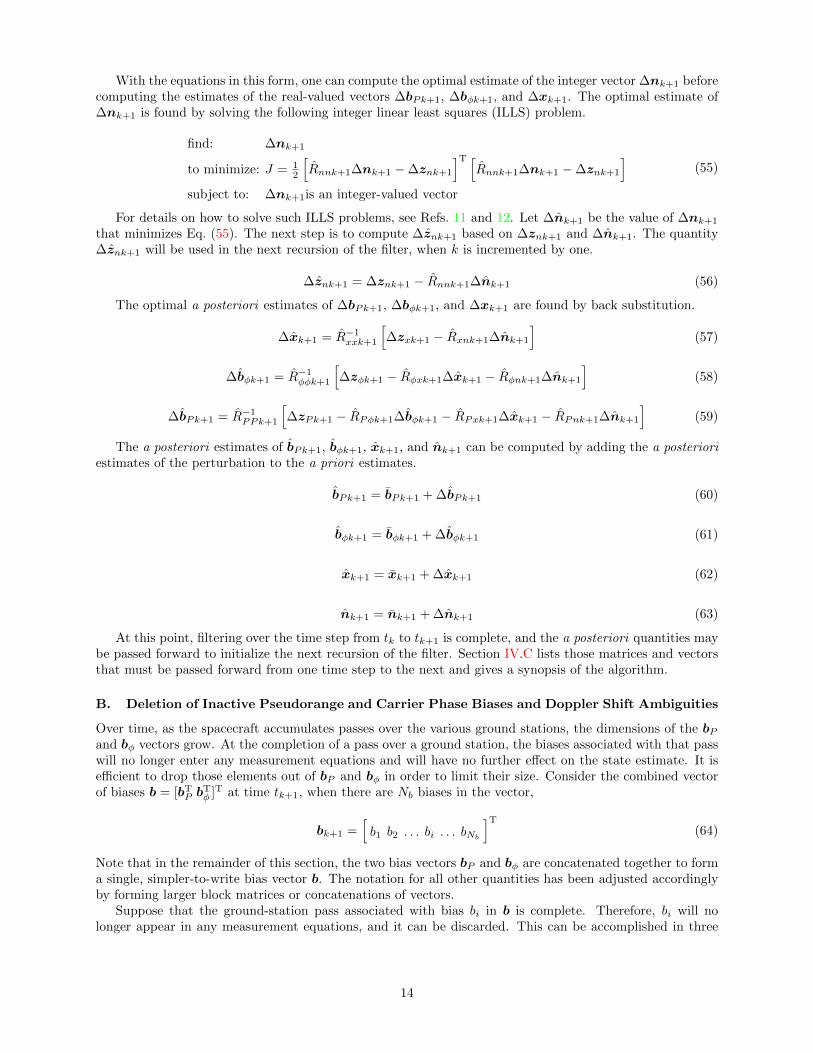
In cases where the Doppler shift ambiguities are estimated exactly correctly, this form of the NEES isequivalent to the standard form given in Eq. 67. If the filter is consistent, each ε(k) should be drawn froma χ2 distribution with nx degrees of freedom, where nx is the number of elements in the state vector, x. Ifε(k) comes from such a distribution, then bounds r1 and r2 can be computed such that ε(k) should fall inthe interval [r1, r2] with some chosen probability. Fig. 4 shows the NEES for a single run of the filter alongwith the 90% probability region plotted on a logarithmic scale. For this particular run, the NEES fell insidethe 90% probability region 97.7% of the time. Over all runs, the NEES fell inside the 90% probability regionbetween 87.2% and 97.7% of the time, with an average of 90.5% of NEES inside the 90% probability region.

The other consistency test that was run is the normalized innovation squared. The NIS is

εν(k) = ∆zres(k)T∆zres(k), (69)

The quantity εν(k) should be drawn from a χ2 distribution with nz(k) degrees of freedom, where nz(k)is the number of measurements that arrive between time tk and time tk+1. Note that were it not for thepresence of integer states, εν(k) would equal the usual NIS, ν(k)TS(k)−1ν(k), where ν(k) is the usual Kalmanfilter innovation and S(k) is its covariance.

As was the case for the NEES, an interval can be defined, based on the properties of the χ2 distribution,in which εν(k) should fall with some probability, if the filter is consistent. Fig. 5 shows an example of the NISduring a single pass over the United States along with the 90% probability region plotted on a logarithmicscale. Note that the bounds of the 90% probability region vary from one time step to the next, because

17

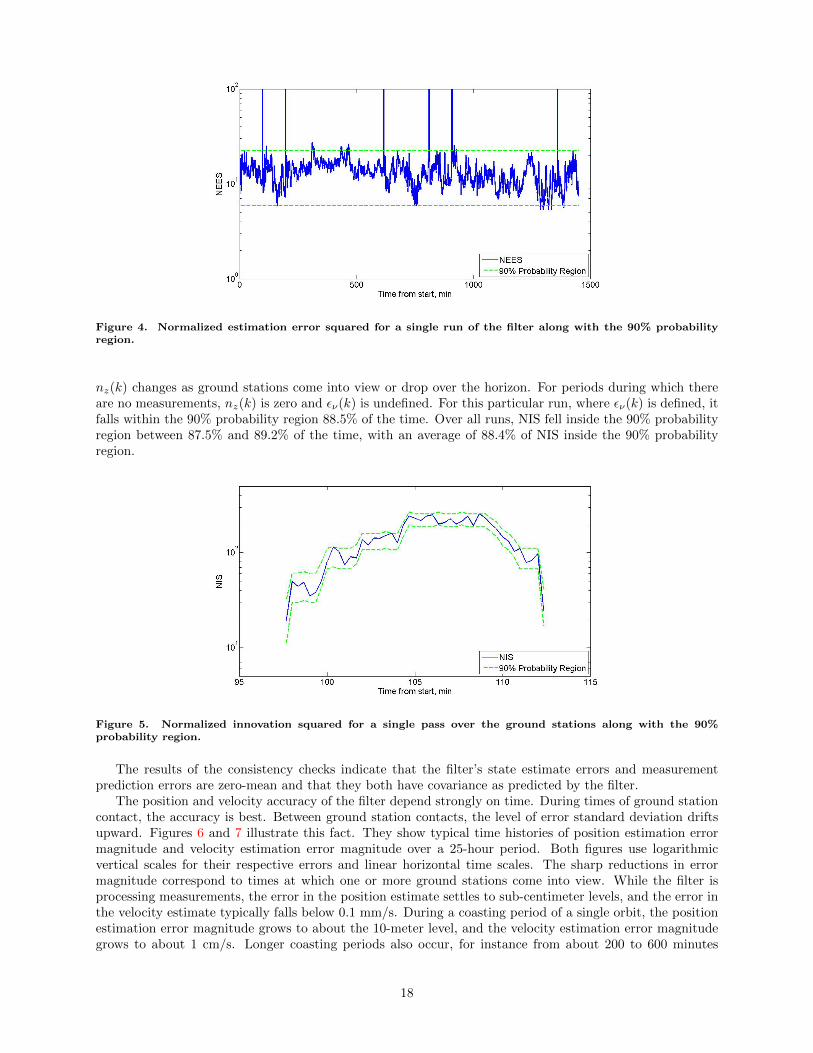
Figure 4. Normalized estimation error squared for a single run of the filter along with the 90% probabilityregion.

nz(k) changes as ground stations come into view or drop over the horizon. For periods during which thereare no measurements, nz(k) is zero and εν(k) is undefined. For this particular run, where εν(k) is defined, itfalls within the 90% probability region 88.5% of the time. Over all runs, NIS fell inside the 90% probabilityregion between 87.5% and 89.2% of the time, with an average of 88.4% of NIS inside the 90% probabilityregion.

Figure 5. Normalized innovation squared for a single pass over the ground stations along with the 90%probability region.

The results of the consistency checks indicate that the filter’s state estimate errors and measurementprediction errors are zero-mean and that they both have covariance as predicted by the filter.

The position and velocity accuracy of the filter depend strongly on time. During times of ground stationcontact, the accuracy is best. Between ground station contacts, the level of error standard deviation driftsupward. Figures 6 and 7 illustrate this fact. They show typical time histories of position estimation errormagnitude and velocity estimation error magnitude over a 25-hour period. Both figures use logarithmicvertical scales for their respective errors and linear horizontal time scales. The sharp reductions in errormagnitude correspond to times at which one or more ground stations come into view. While the filter isprocessing measurements, the error in the position estimate settles to sub-centimeter levels, and the error inthe velocity estimate typically falls below 0.1 mm/s. During a coasting period of a single orbit, the positionestimation error magnitude grows to about the 10-meter level, and the velocity estimation error magnitudegrows to about 1 cm/s. Longer coasting periods also occur, for instance from about 200 to 600 minutes

18

in Fig. 6, which correspond to about four full orbits. During these long coasting periods, across all runsconsidered, the position estimation error grew to a maximum of 681.3 m with an average of 305.5 m.

The same data that went into Fig. 6 are broken into their along-track, altitude, and cross-track compo-nents and re-plotted in Fig. 8. As expected, the orbit plane is determined very well; the peak cross-trackposition estimate error in this run, after the initial transient, is only 2.1 meters and 0.10 meters RMS. Alsoas expected, it is the along-track direction with the highest estimation error—about 681.3 meters followingthe first long coasting period, but only 201 meters RMS. The maximum and RMS position estimation errorsare summarized in Table 1. Note that these errors are all calculated after waiting for the initial transient todie out.

Figure 6. Position error magnitude time history for a typical 25-hour period.

Figure 7. Velocity error magnitude time history for a typical 25-hour period.

Note that the best results here, with position accuracy better than 1 cm and velocity accuracy betterthan 0.1 mm/s are over optimistic. When real effects are considered that are not presently modeled, theaccuracy will degrade. Such effects include residual force model errors, as well as errors in models of theionospheric and neutral atmosphere delays.

19

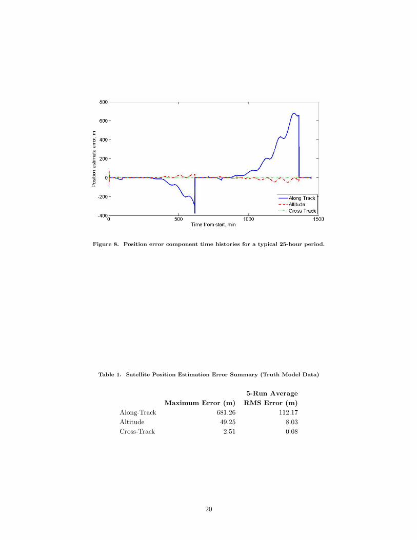
Figure 8. Position error component time histories for a typical 25-hour period.

Table 1. Satellite Position Estimation Error Summary (Truth Model Data)

5-Run Average

Maximum Error (m) RMS Error (m)

Along-Track 681.26 112.17

Altitude 49.25 8.03

Cross-Track 2.51 0.08

20

VII. Summary and Conclusions

A new Kalman filtering technique was applied in an orbit determination setting using time-divisionmultiple access (TDMA) radio communication signals that were not originally intended for this application.The orbit determination filter has two significant new features. The first is an ability to deal directlyand consistently with the unknown measurement effectiveness times that result from using ground-basedradio navigation data. The second new feature is the estimation of integer Doppler shift ambiguities. Suchambiguities tend to arise for TDMA signals. The implicit nature of the measurement effectiveness times wasdealt with by using dense-output Runge-Kutta numerical integration throughout to provide interpolatedvalues for the state at all times. This feature also required the use of a piecewise polynomial process noisemodel. In order to handle the integer-valued Doppler shift ambiguities in a sensible way, the square-rootinformation extended Kalman filter solved an integer linear least squares problem before estimating thereal-valued portion of the state vector.

In truth model simulation, the algorithm determines the orbits of low Earth orbit satellites with RMSposition error magnitude of only 110 meters overall. The peak position error magnitude observed of about680 meters occurs after nearly 7 hours without measurements. Statistical consistency checks on the stateestimation errors and the residuals showed that the filter functions as expected. If the periods during whichno measurements were available were shortened by increasing the number and geographical diversity ofground stations, the peak position estimate errors could be reduced significantly. Longer filtering runs mightalso reduce this error.

References

1Mohiuddin, S. and Psiaki, M. L., “Continuous-Time Kalman Filtering with Implicit Discrete Measurement Times,” AIAAGuidance, Navigation, and Control Conference, Washington, D.C., Aug. 2009, pp. 4574–4607.

2Psiaki, M. L., “Kalman Filtering and Smoothing to Estimate Real-Valued States and Integer Constants,” AIAA Guidance,Navigation, and Control Conference Proceedings, Washington, D.C., Aug. 2009, AIAA Paper Number 2009-5972.

3Brown, R. G. and Hwang, P. Y. C., Introduction to Random Signals and Applied Kalman Filtering with MATLABexercises and solutions, Wiley, New York, 3rd ed., Nov. 1996.

4Lundberg, J. and Schutz, B., “Recursion Formulas for Legendre Functions for Use with Nonsingular Geopotential Models,”Journal of Guidance, Control, and Dynamics, Vol. 11, No. 1, January–February 1988, pp. 31–38.

5Montenbruck, O. and Gill, E., Satellite Orbits: Models, Methods and Applications, Springer, Berlin, Heidelberg, andNew York, 2005.

6Nørsett, S. P., Wanner, G., and Hairer, E., Solving ordinary differential equations, Springer-Verlag, Berlin, 1987.7Mendes, V., Modeling the Neutral-Atmospheric Propagation Delay in Radiometric Space Techniques, Ph.D. thesis,

Geodesy and Geomatics Engineering, University of New Brunswick, April 1999.8Misra, P. and Enge, P., Global Positioning System: Signals, Measurements, and Performance, Ganga-Jamuna Press,

Lincoln, Massachusetts, 2nd ed., 2006.9Bierman, G. J., Factorization Methods for Discrete Sequential Estimation, Academic Press, New York, New York, 1977,

pp 69–76, 115–122, 214–217.10Gill, P. E., Murray, W., and Wright, M. H., Practical Optimization, Academic Press, San Diego, California, 1981, pp

37–40.11Teunissen, P. J. G., “The Least-Squares Ambiguity Decorrelation Adjustment: A Method for Fast GPS Integer Ambiguity

Estimation,” Journal of Geodesy, Vol. 70, No. 1–2, Nov. 1995, pp. 65–82.12Psiaki, M. and Mohiuddin, S., “Global Positioning System Integer Ambiguity Resolution Using Factorized Least Squares

Techniques,” Journal of Guidance, Control, and Dynamics, Vol. 30, No. 2, Mar–Apr 2007, pp. 346–356.13Bar-Shalom, Y., Li, X. R., and Kirubarajan, T., Estimation with Applications to Tracking and Navigation, John Wiley

and Sons, New York, New York, 2001, pp 232–236.

21