ORANI-G A Generic CGE Model
198
1 ORANI-G A Generic CGE Model Document: ORANI-G: a Generic Single-Country Computable General Equilibrium Model Please tell me if you find any mistakes in the document ! Oranig06.ppt
Transcript of ORANI-G A Generic CGE Model

1
ORANI-GA Generic CGE Model
Document: ORANI-G: a Generic Single-Country
Computable General Equilibrium ModelPlease tell me if you find any mistakes in the document !
Oranig06.ppt
2
Contents
Introduction Inventory demands
Database structure Margin demands
Solution method Market clearing
TABLO language Price equations
Production: input decisions Aggregates and indices
Production: output decisions Investment allocation
Investment: input decisions Labour market
Household demands Decompositions
Export demands Closure
Government demands Regional extension
3
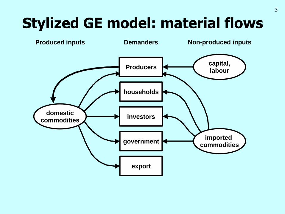
Stylized GE model: material flows
Producers
imported commodities
export
households
investors
government
domesticcommodities
capital,labour
Demanders Non-produced inputsProduced inputs
4
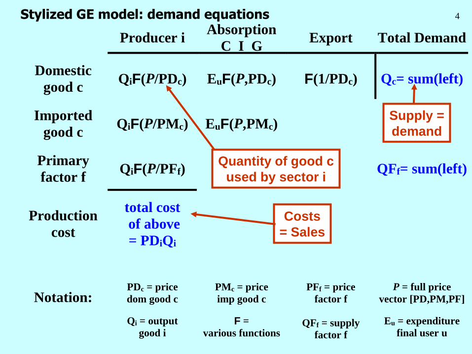
Producer iAbsorption
C I GExport Total Demand
Domestic
good cQiF(P/PDc) EuF(P,PDc) F(1/PDc) Qc= sum(left)
Imported
good cQiF(P/PMc) EuF(P,PMc)
Primary
factor fQiF(P/PFf) QFf= sum(left)
Production
cost
total cost
of above
= PDiQi
Notation:PDc = price
dom good c
PMc = price
imp good c
PFf = price
factor f
P = full price
vector [PD,PM,PF]
Qi = output
good i
F =
various functionsQFf = supply
factor f
Eu = expenditure
final user u
Supply =
demand
Costs
= Sales
Quantity of good c
used by sector i
Stylized GE model: demand equations
5
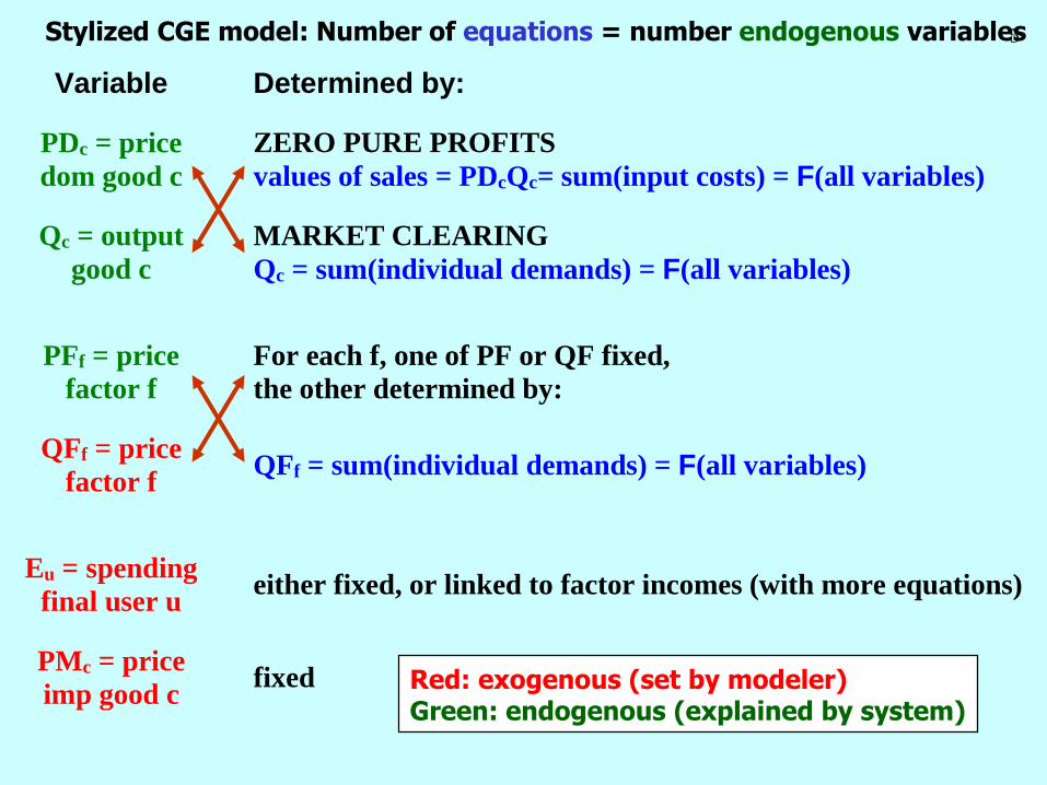
Variable Determined by:
PDc = price
dom good c
ZERO PURE PROFITS
values of sales = PDcQc= sum(input costs) = F(all variables)
Qc = output
good c
MARKET CLEARING
Qc = sum(individual demands) = F(all variables)
PFf = price
factor f
For each f, one of PF or QF fixed,
the other determined by:
QFf = price
factor fQFf = sum(individual demands) = F(all variables)
Eu = spending
final user ueither fixed, or linked to factor incomes (with more equations)
PMc = price
imp good cfixed
Stylized CGE model: Number of equations = number endogenous variables
Red: exogenous (set by modeler)Green: endogenous (explained by system)
6
What is an applied CGE model ?
Computable, based on data
It has many sectors
And perhaps many regions, primary factors and
households
A big database of matrices
Many, simultaneous, equations (hard to solve)
Prices guide demands by agents
Prices determined by supply and demand
Trade focus: elastic foreign demand and supply
7
CGE simplifications
Not much dynamics (leads and lags)
An imposed structure of behaviour, based on theory
Neoclassical assumptions (optimizing, competition)
Nesting (separability assumptions)
Why: time series data for huge matrices cannot be found.
Theory and assumptions (partially) replace econometrics

8
What is a CGE model good for ?
Analysing policies that affect different sectors in
different ways
The effect of a policy on different:
Sectors
Regions
Factors (Labour, Land, Capital)
Household types
Policies (tariff or subsidies) that help one sector a lot,
and harm all the rest a little.
9
What-if questions
What if productivity in agriculture increased 1%?
What if foreign demand for exports increased 5%?
What if consumer tastes shifted towards imported food?
What if CO2 emissions were taxed?
What if water became scarce?
A great number of exogenous variables (tax rates,
endowments, technical coefficients).
Comparative static models: Results show effect of policy
shocks only, in terms of changes from initial equilibrium
10
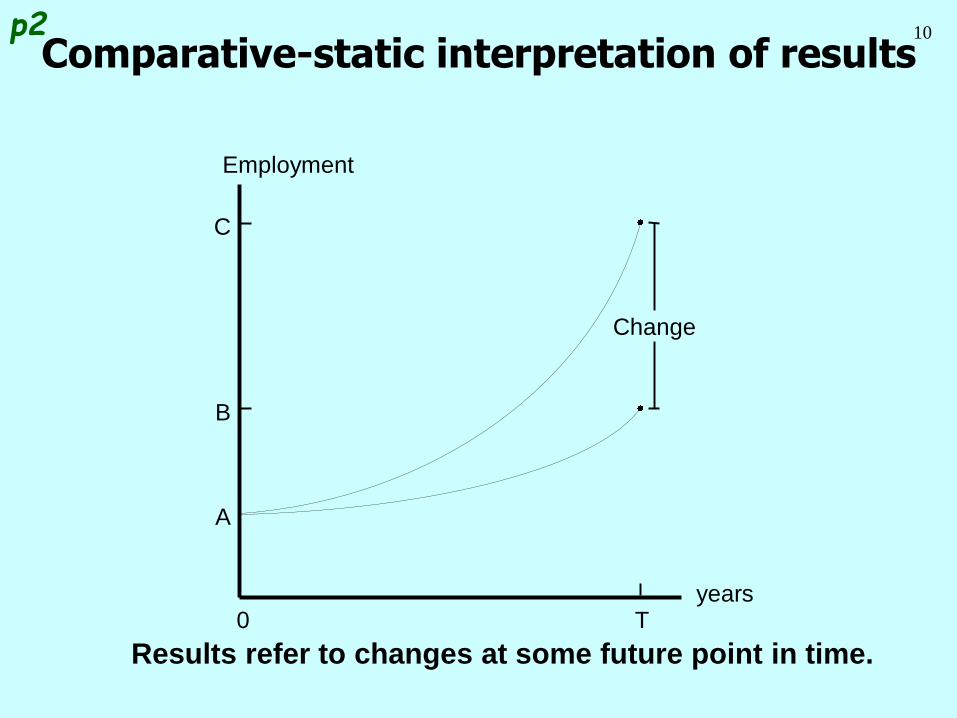
Comparative-static interpretation of results
Results refer to changes at some future point in time.
Employment
0 T
Change
A
years
B
C
p2
11
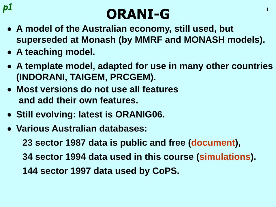
ORANI-Gp1
A model of the Australian economy, still used, but
superseded at Monash (by MMRF and MONASH models).
A teaching model.
A template model, adapted for use in many other countries
(INDORANI, TAIGEM, PRCGEM).
Most versions do not use all features
and add their own features.
Still evolving: latest is ORANIG06.
Various Australian databases:
23 sector 1987 data is public and free (document),
34 sector 1994 data used in this course (simulations).
144 sector 1997 data used by CoPS.
12
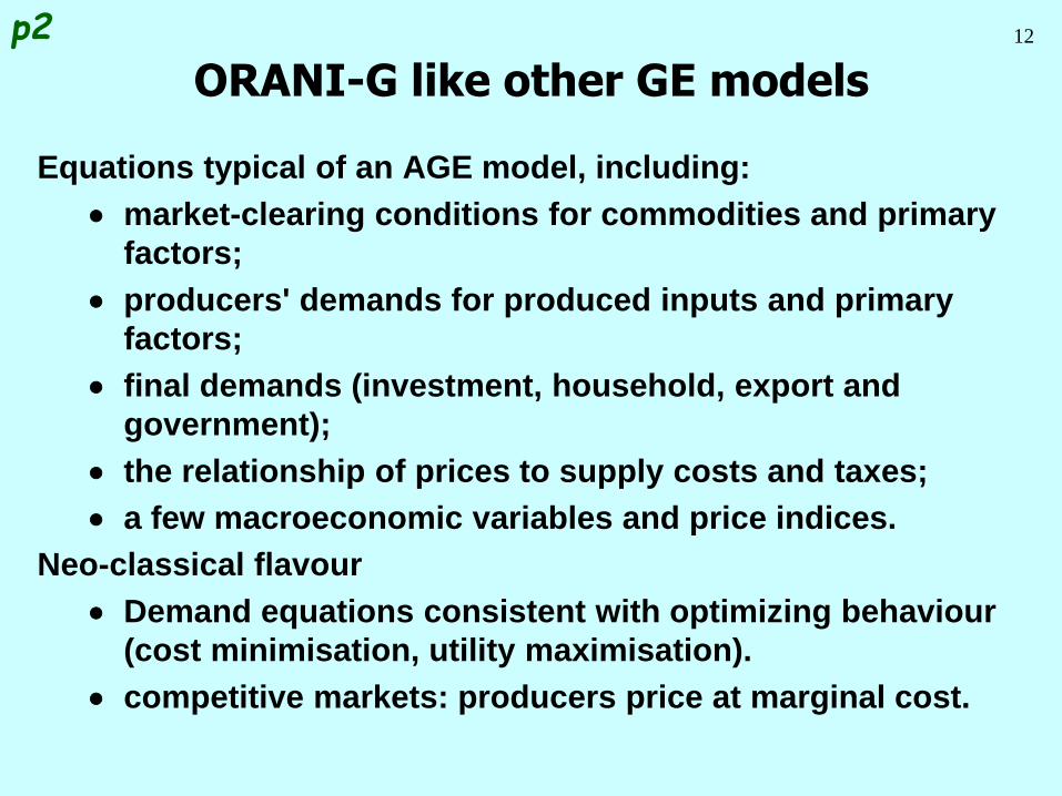
ORANI-G like other GE models
Equations typical of an AGE model, including:
market-clearing conditions for commodities and primary
factors;
producers' demands for produced inputs and primary
factors;
final demands (investment, household, export and
government);
the relationship of prices to supply costs and taxes;
a few macroeconomic variables and price indices.
Neo-classical flavour
Demand equations consistent with optimizing behaviour
(cost minimisation, utility maximisation).
competitive markets: producers price at marginal cost.
p2
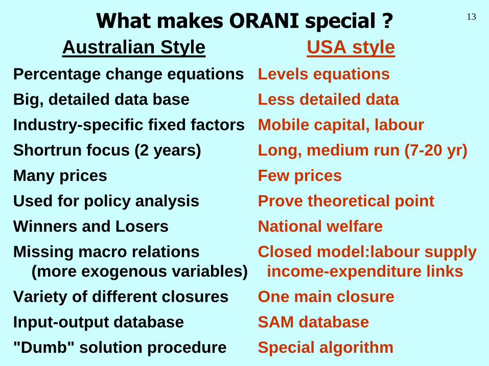
13What makes ORANI special ?
Australian Style USA style
Percentage change equations Levels equations
Big, detailed data base Less detailed data
Industry-specific fixed factors Mobile capital, labour
Shortrun focus (2 years) Long, medium run (7-20 yr)
Many prices Few prices
Used for policy analysis Prove theoretical point
Winners and Losers National welfare
Missing macro relations Closed model:labour supply
(more exogenous variables) income-expenditure links
Variety of different closures One main closure
Input-output database SAM database
"Dumb" solution procedure Special algorithm
14
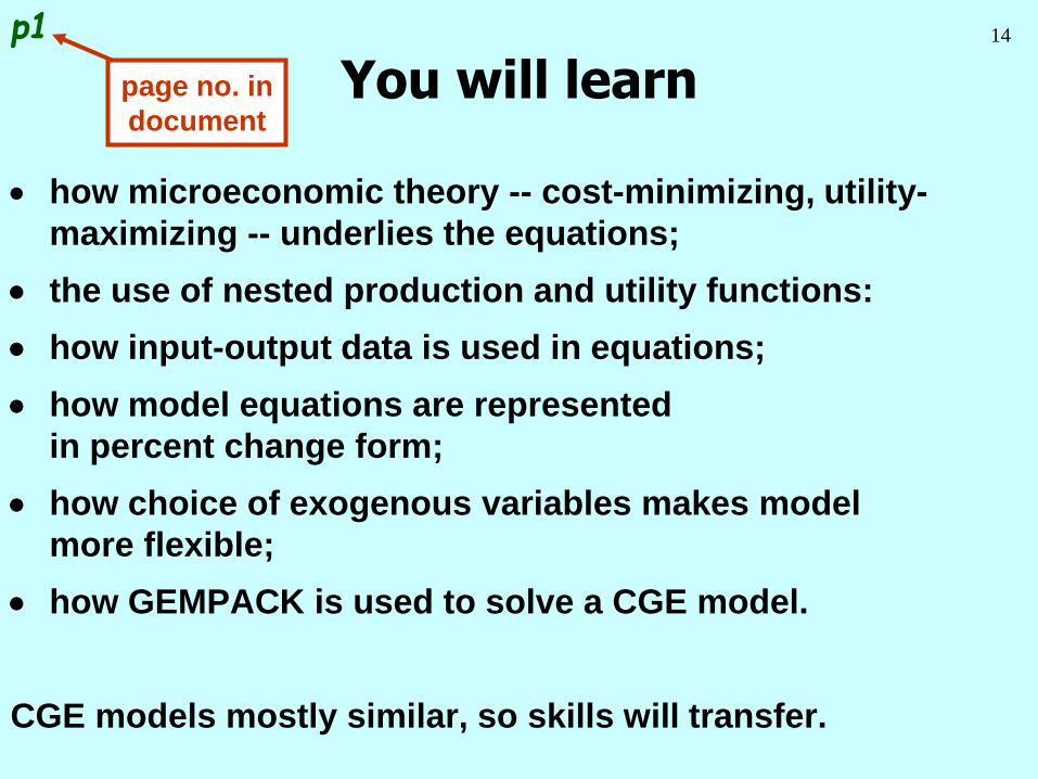
You will learn
how microeconomic theory -- cost-minimizing, utility-
maximizing -- underlies the equations;
the use of nested production and utility functions:
how input-output data is used in equations;
how model equations are represented
in percent change form;
how choice of exogenous variables makes model
more flexible;
how GEMPACK is used to solve a CGE model.
CGE models mostly similar, so skills will transfer.
p1
page no. in
document
15
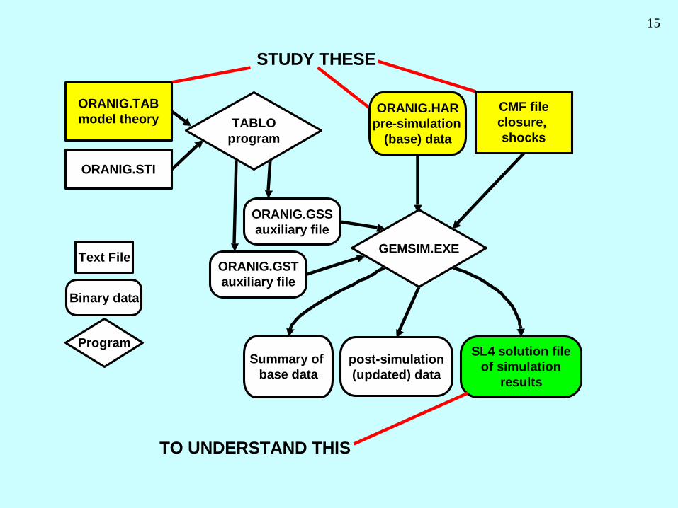
ORANIG.GST
auxiliary file
ORANIG.GSS
auxiliary file
GEMSIM.EXE
CMF file
closure,
shocks
ORANIG.HAR
pre-simulation
(base) data
SL4 solution file
of simulation
results
Summary of
base data
post-simulation
(updated) data
ORANIG.TAB
model theory
ORANIG.STI
TABLO
program
Binary data
Program
Text File
STUDY THESE
TO UNDERSTAND THIS
16
Progress so far . . .
Introduction Inventory demands
Database structure Margin demands
Solution method Market clearing
TABLO language Price equations
Production: input decisions Aggregates and indices
Production: output decisions Investment allocation
Investment: input decisions Labour market
Household demands Decompositions
Export demands Closure
Government demands Regional extension
17
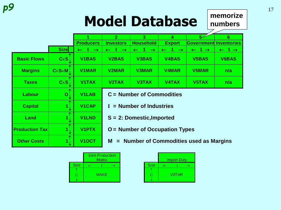
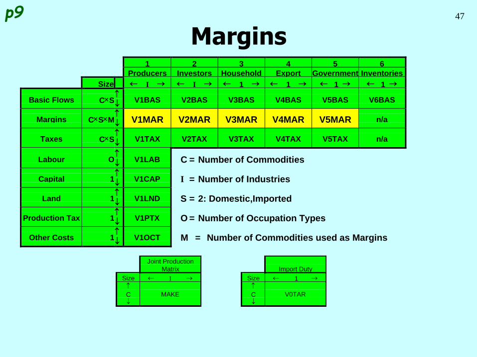
Model Database1 2 3 4 5 6
Producers Investors Household Export Government Inventories
Size I I 1 1 1 1
Basic Flows CS
V1BAS V2BAS V3BAS V4BAS V5BAS V6BAS
Margins CSM
V1MAR V2MAR V3MAR V4MAR V5MAR n/a
Taxes CS
V1TAX V2TAX V3TAX V4TAX V5TAX n/a
Labour O
V1LAB C = Number of Commodities
Capital 1
V1CAP I = Number of Industries
Land 1
V1LND S = 2: Domestic,Imported
Production Tax 1
V1PTX O = Number of Occupation Types
Other Costs 1
V1OCT M = Number of Commodities used as Margins
Joint ProductionMatrix Import Duty
Size I Size 1
C
MAKE
C
V0TAR
p9memorize
numbers
18
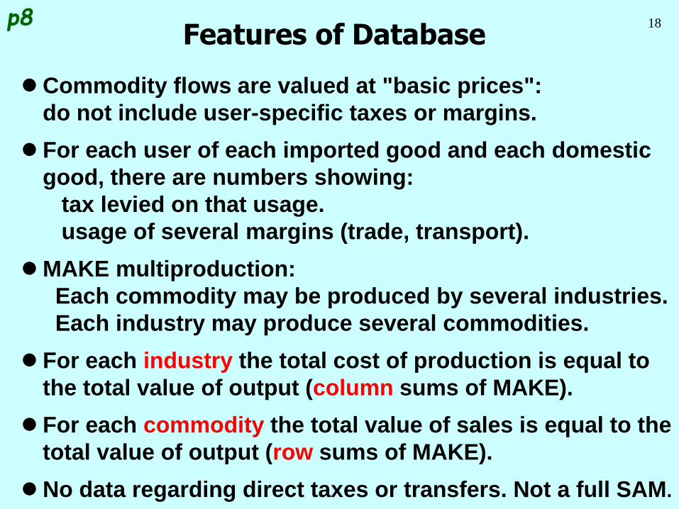
Features of Database
Commodity flows are valued at "basic prices":
do not include user-specific taxes or margins.
For each user of each imported good and each domestic
good, there are numbers showing:
tax levied on that usage.
usage of several margins (trade, transport).
MAKE multiproduction:
Each commodity may be produced by several industries.
Each industry may produce several commodities.
For each industry the total cost of production is equal to
the total value of output (column sums of MAKE).
For each commodity the total value of sales is equal to the
total value of output (row sums of MAKE).
No data regarding direct taxes or transfers. Not a full SAM.
p8
19
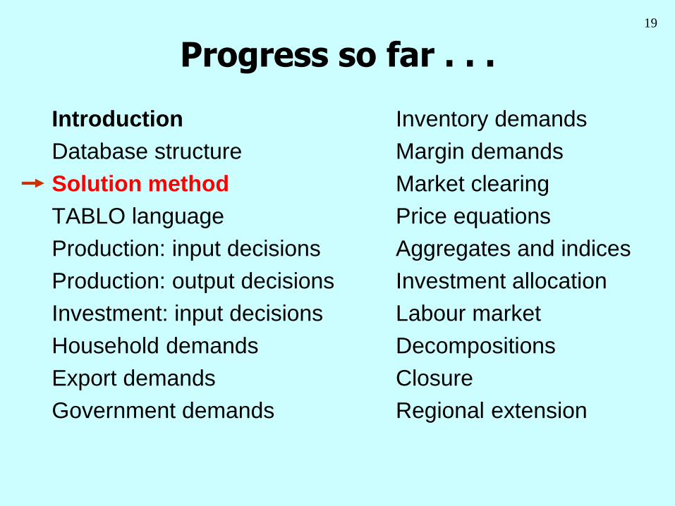
Progress so far . . .
Introduction Inventory demands
Database structure Margin demands
Solution method Market clearing
TABLO language Price equations
Production: input decisions Aggregates and indices
Production: output decisions Investment allocation
Investment: input decisions Labour market
Household demands Decompositions
Export demands Closure
Government demands Regional extension
20
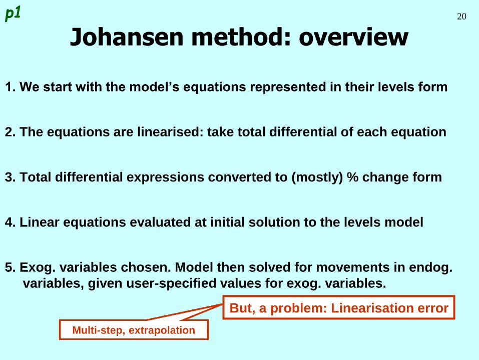
Johansen method: overview
1. We start with the model’s equations represented in their levels form
2. The equations are linearised: take total differential of each equation
3. Total differential expressions converted to (mostly) % change form
4. Linear equations evaluated at initial solution to the levels model
5. Exog. variables chosen. Model then solved for movements in endog.
variables, given user-specified values for exog. variables.
p1
But, a problem: Linearisation error
Multi-step, extrapolation
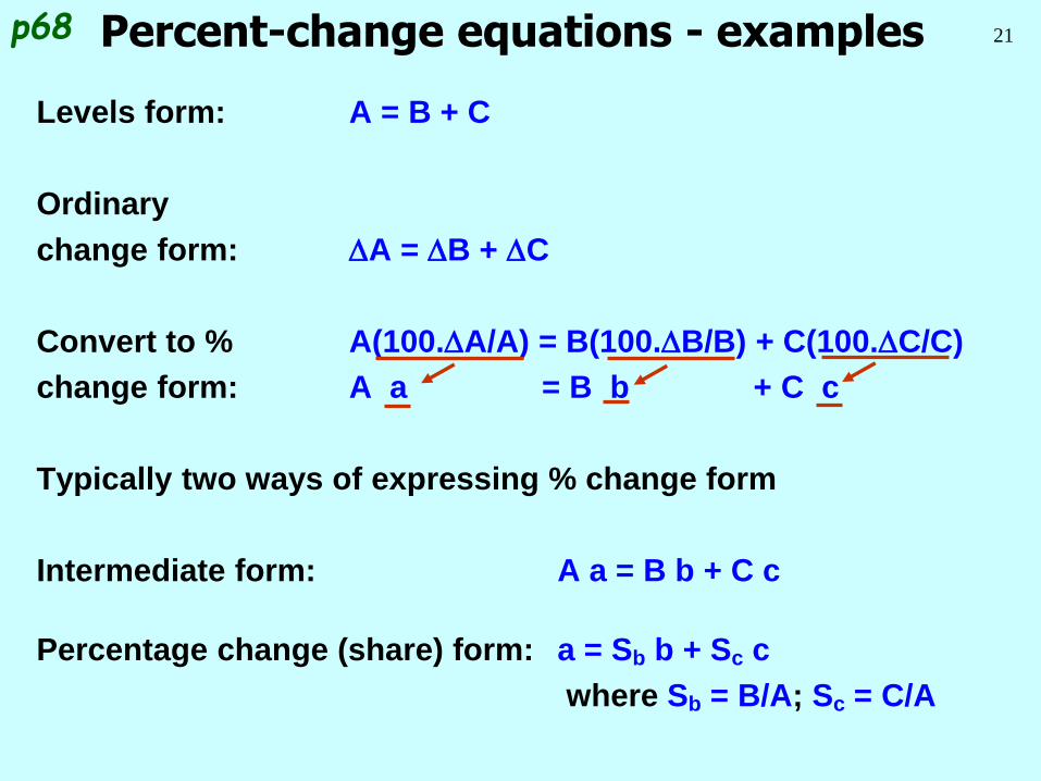
21Percent-change equations - examples
Levels form: A = B + C
Ordinary
change form: DA = DB + DC
Convert to % A(100.DA/A) = B(100.DB/B) + C(100.DC/C)
change form: A a = B b + C c
Typically two ways of expressing % change form
Intermediate form: A a = B b + C c
Percentage change (share) form: a = Sb b + Sc c
where Sb = B/A; Sc = C/A
p68
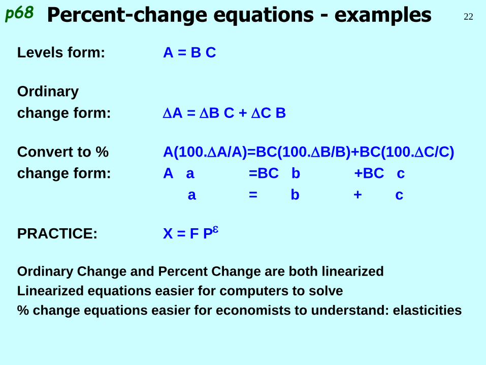
22Percent-change equations - examples
Levels form: A = B C
Ordinary
change form: DA = DB C + DC B
Convert to % A(100.DA/A)=BC(100.DB/B)+BC(100.DC/C)
change form: A a =BC b +BC c
a = b + c
PRACTICE: X = F Pe
Ordinary Change and Percent Change are both linearized
Linearized equations easier for computers to solve
% change equations easier for economists to understand: elasticities
p68
23
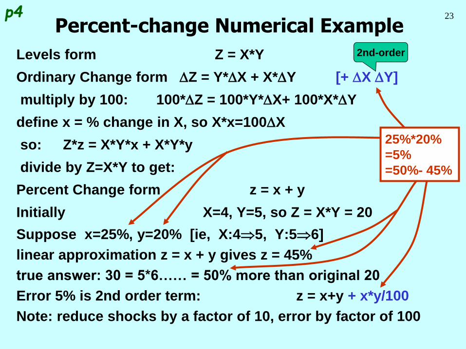
Percent-change Numerical Example
Levels form Z = X*Y
Ordinary Change form DZ = Y*DX + X*DY [+ DX DY]
multiply by 100: 100*DZ = 100*Y*DX+ 100*X*DY
define x = % change in X, so X*x=100DX
so: Z*z = X*Y*x + X*Y*y
divide by Z=X*Y to get:
Percent Change form z = x + y
Initially X=4, Y=5, so Z = X*Y = 20
Suppose x=25%, y=20% [ie, X:45, Y:56]
linear approximation z = x + y gives z = 45%
true answer: 30 = 5*6…… = 50% more than original 20
Error 5% is 2nd order term: z = x+y + x*y/100
Note: reduce shocks by a factor of 10, error by factor of 100
2nd-order
p4
25%*20%
=5%
=50%- 45%
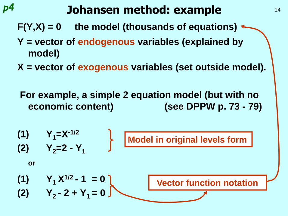
24Johansen method: example
F(Y,X) = 0 the model (thousands of equations)
Y = vector of endogenous variables (explained by
model)
X = vector of exogenous variables (set outside model).
For example, a simple 2 equation model (but with no
economic content) (see DPPW p. 73 - 79)
(1) Y1=X-1/2
(2) Y2=2 - Y1
or
(1) Y1 X1/2 - 1 = 0
(2) Y2 - 2 + Y1 = 0
p4
Vector function notation
Model in original levels form
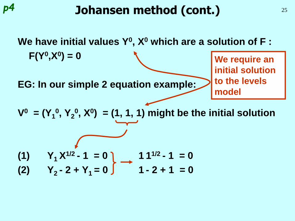
25Johansen method (cont.)
We have initial values Y0, X0 which are a solution of F :
F(Y0,X0) = 0
EG: In our simple 2 equation example:
V0 = (Y10, Y2
0, X0) = (1, 1, 1) might be the initial solution
(1) Y1 X1/2 - 1 = 0 1 11/2 - 1 = 0
(2) Y2 - 2 + Y1 = 0 1 - 2 + 1 = 0
p4
We require an
initial solution
to the levels
model
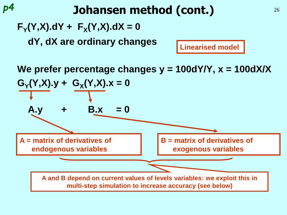
26Johansen method (cont.)
FY(Y,X).dY + FX(Y,X).dX = 0
dY, dX are ordinary changes
We prefer percentage changes y = 100dY/Y, x = 100dX/X
GY(Y,X).y + GX(Y,X).x = 0
A.y + B.x = 0
p4
B = matrix of derivatives of
exogenous variables
A = matrix of derivatives of
endogenous variables
A and B depend on current values of levels variables: we exploit this in
multi-step simulation to increase accuracy (see below)
Linearised model
27Johansen method (cont.)
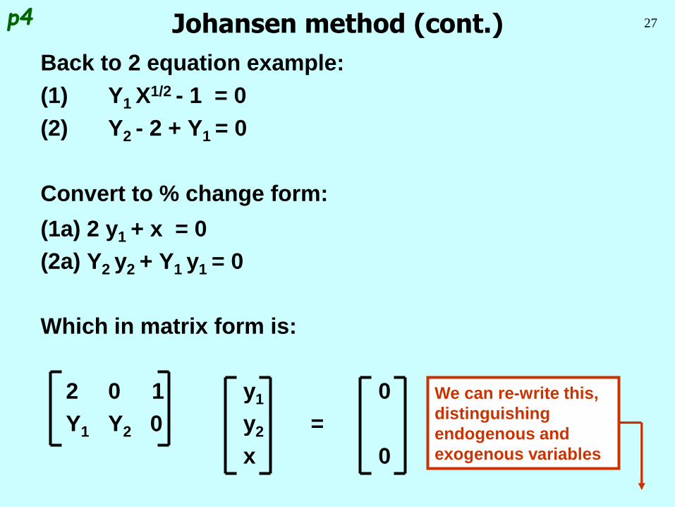
Back to 2 equation example:
(1) Y1 X1/2 - 1 = 0
(2) Y2 - 2 + Y1 = 0
Convert to % change form:
(1a) 2 y1 + x = 0
(2a) Y2 y2 + Y1 y1 = 0
Which in matrix form is:
2 0 1 y1 0
Y1 Y2 0 y2 =
x 0
p4
We can re-write this,
distinguishing
endogenous and
exogenous variables
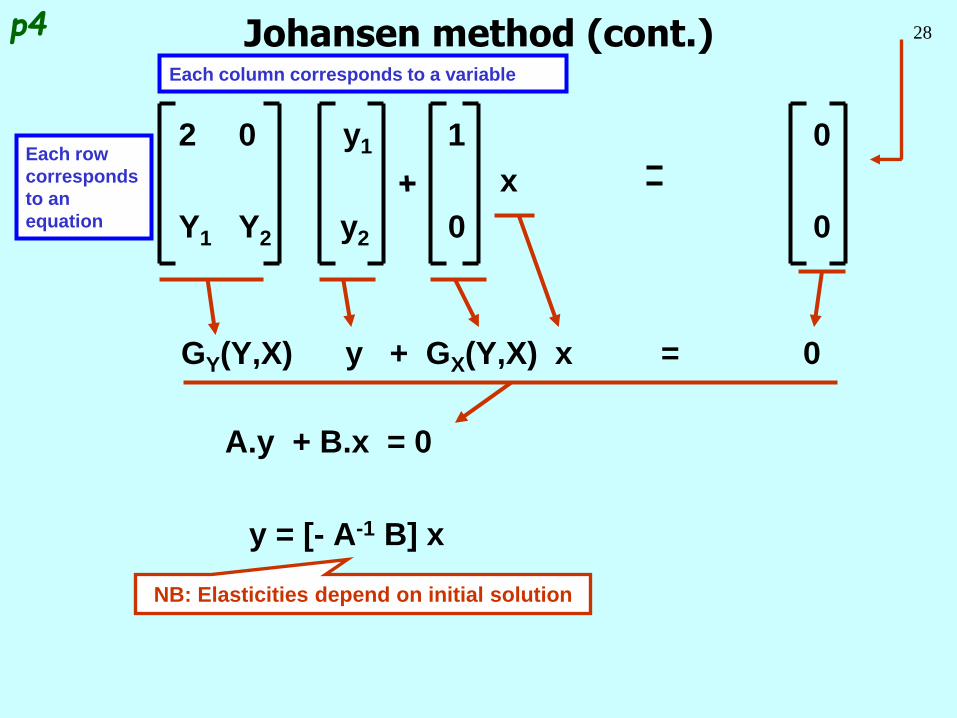
28Johansen method (cont.)
2 0 y1 1 0
x
Y1 Y2 y2 0 0
GY(Y,X) y + GX(Y,X) x = 0
A.y + B.x = 0
y = [- A-1 B] x
p4
Each row
corresponds
to an
equation
Each column corresponds to a variable
NB: Elasticities depend on initial solution
29Johansen method (cont.)
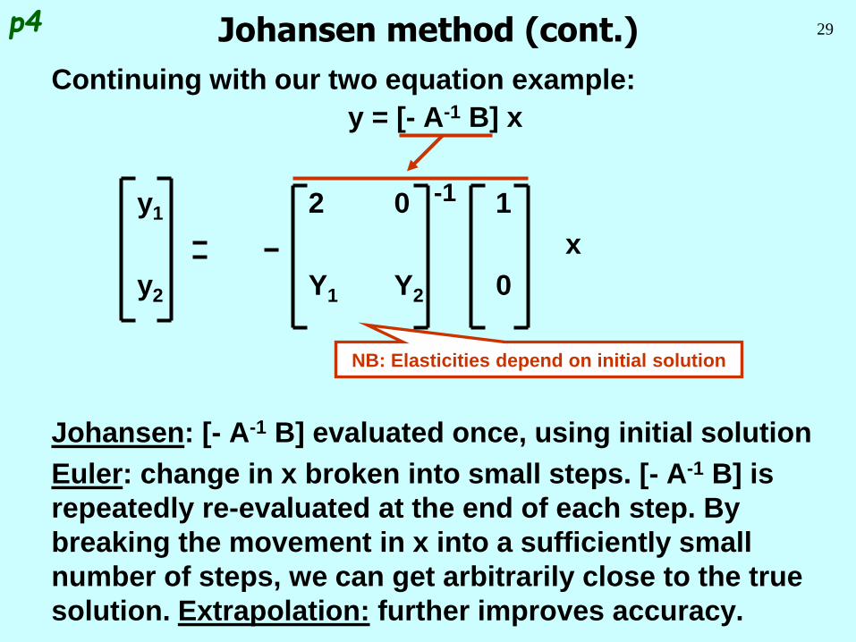
Continuing with our two equation example:
y = [- A-1 B] x
y1 2 0 -1 1
x
y2 Y1 Y2 0
Johansen: [- A-1 B] evaluated once, using initial solution
Euler: change in x broken into small steps. [- A-1 B] is
repeatedly re-evaluated at the end of each step. By
breaking the movement in x into a sufficiently small
number of steps, we can get arbitrarily close to the true
solution. Extrapolation: further improves accuracy.
p4
NB: Elasticities depend on initial solution
30
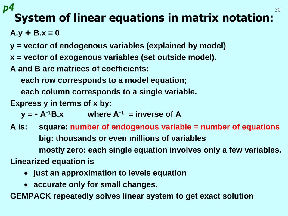
System of linear equations in matrix notation:
A.y + B.x = 0
y = vector of endogenous variables (explained by model)
x = vector of exogenous variables (set outside model).
A and B are matrices of coefficients:
each row corresponds to a model equation;
each column corresponds to a single variable.
Express y in terms of x by:
y = - A-1B.x where A-1 = inverse of A
A is: square: number of endogenous variable = number of equations
big: thousands or even millions of variables
mostly zero: each single equation involves only a few variables.
Linearized equation is
just an approximation to levels equation
accurate only for small changes.
GEMPACK repeatedly solves linear system to get exact solution
p4
31
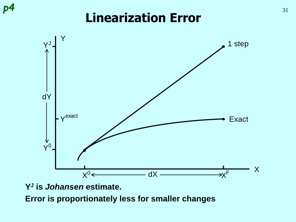
Linearization Error
YJ is Johansen estimate.
Error is proportionately less for smaller changes
Y1 step
Exact
XX0 X
Y0
Yexact
F
YJ
dX
dY
p4
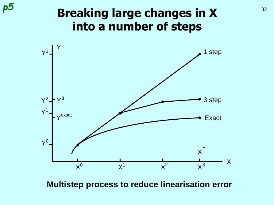
32Breaking large changes in X
into a number of steps
Multistep process to reduce linearisation error
Y1 step
3 step
Exact
XX0 X1 X
2X3
Y0
Y1
Y3
Yexact
Y2
XF
YJ
p5
33
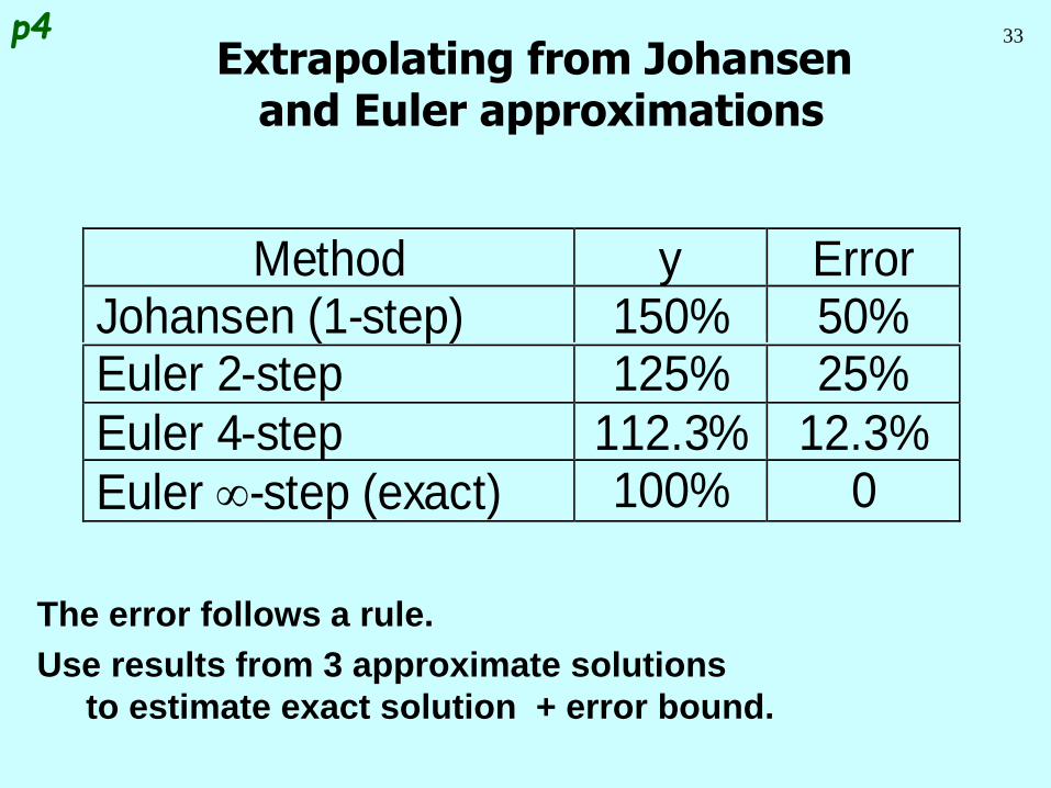
Extrapolating from Johansenand Euler approximations
The error follows a rule.
Use results from 3 approximate solutions
to estimate exact solution + error bound.
Method y ErrorJohansen (1-step) 150% 50%Euler 2-step 125% 25%
Euler 4-step 112.3% 12.3%
Euler -step (exact) 100% 0
p4
34
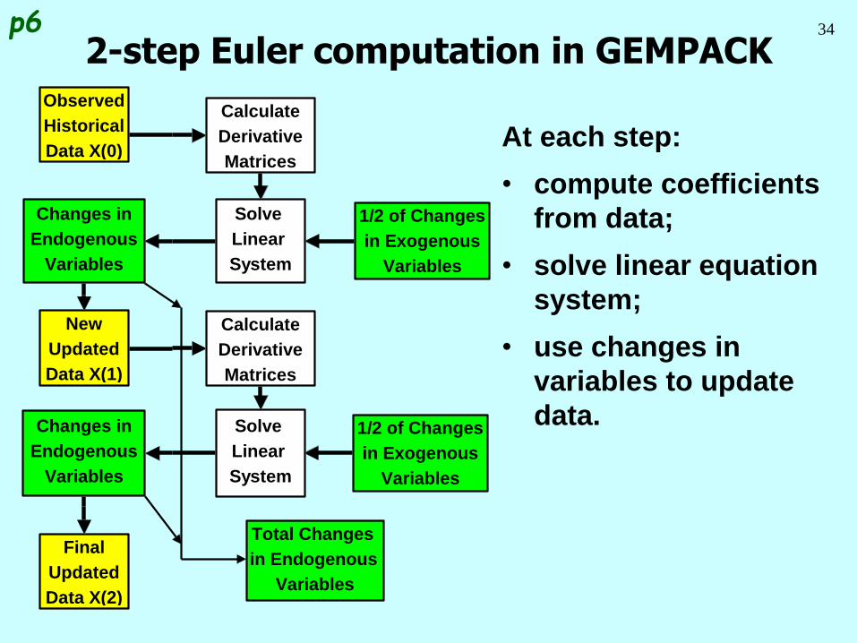
2-step Euler computation in GEMPACK
At each step:
• compute coefficients
from data;
• solve linear equation
system;
• use changes in
variables to update
data.
Total Changes
in Endogenous
Variables
Final
Updated
Data X(2)
Changes in
Endogenous
Variables
Solve
Linear
System
1/2 of Changes
in Exogenous
Variables
Calculate
Derivative
Matrices
New
Updated
Data X(1)
Changes in
Endogenous
Variables
Solve
Linear
System
1/2 of Changes
in Exogenous
Variables
Calculate
Derivative
Matrices
Observed
Historical
Data X(0)
p6
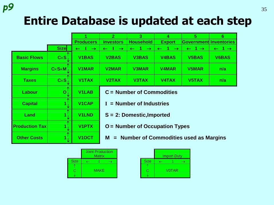
35
Entire Database is updated at each step1 2 3 4 5 6
Producers Investors Household Export Government Inventories
Size I I 1 1 1 1
Basic Flows CS
V1BAS V2BAS V3BAS V4BAS V5BAS V6BAS
Margins CSM
V1MAR V2MAR V3MAR V4MAR V5MAR n/a
Taxes CS
V1TAX V2TAX V3TAX V4TAX V5TAX n/a
Labour O
V1LAB C = Number of Commodities
Capital 1
V1CAP I = Number of Industries
Land 1
V1LND S = 2: Domestic,Imported
Production Tax 1
V1PTX O = Number of Occupation Types
Other Costs 1
V1OCT M = Number of Commodities used as Margins
Joint ProductionMatrix Import Duty
Size I Size 1
C
MAKE
C
V0TAR
p9
36
Progress so far . . .
Introduction Inventory demands
Database structure Margin demands
Solution method Market clearing
TABLO language Price equations
Production: input decisions Aggregates and indices
Production: output decisions Investment allocation
Investment: input decisions Labour market
Household demands Decompositions
Export demands Closure
Government demands Regional extension
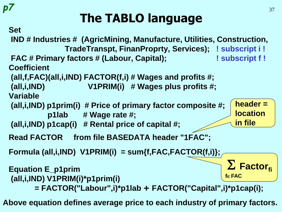
37
The TABLO languageSet
IND # Industries # (AgricMining, Manufacture, Utilities, Construction,
TradeTranspt, FinanProprty, Services); ! subscript i !
FAC # Primary factors # (Labour, Capital); ! subscript f !
Coefficient
(all,f,FAC)(all,i,IND) FACTOR(f,i) # Wages and profits #;
(all,i,IND) V1PRIM(i) # Wages plus profits #;
Variable
(all,i,IND) p1prim(i) # Price of primary factor composite #;
p1lab # Wage rate #;
(all,i,IND) p1cap(i) # Rental price of capital #;
Read FACTOR from file BASEDATA header "1FAC";
Formula (all,i,IND) V1PRIM(i) = sum{f,FAC,FACTOR(f,i)};
Equation E_p1prim
(all,i,IND) V1PRIM(i)*p1prim(i)
= FACTOR("Labour",i)*p1lab + FACTOR("Capital",i)*p1cap(i);
Above equation defines average price to each industry of primary factors.
SFactorfifFAC
p7
header =
location
in file
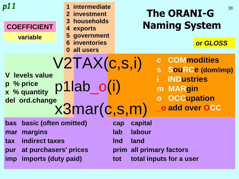
38
The ORANI-GNaming System
p11
c COMmodities
s SouRCe (dom/imp)
i INDustries
m MARgin
o OCCupation
_o add over OCC
V levels value
p % price
x % quantity
del ord.change
1 intermediate2 investment3 households4 exports5 government6 inventories0 all users
cap capital
lab labour
lnd land
prim all primary factors
tot total inputs for a user
COEFFICIENT
or GLOSSvariable
V2TAX(c,s,i)
p1lab_o(i)
x3mar(c,s,m)bas basic (often omitted)
mar margins
tax indirect taxes
pur at purchasers' prices
imp imports (duty paid)
39
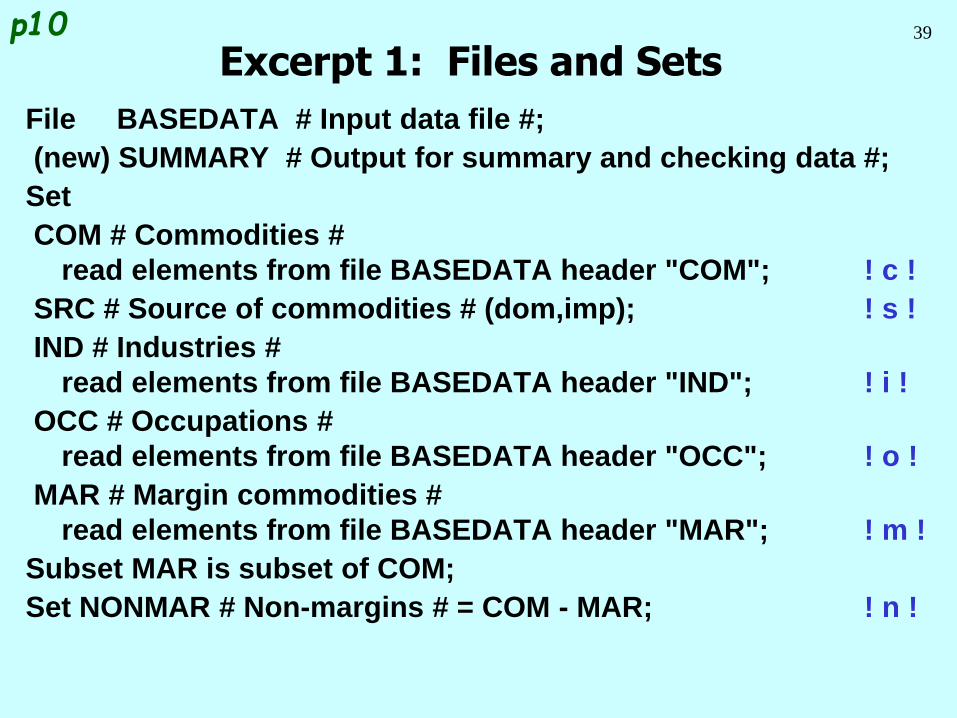
Excerpt 1: Files and Sets
File BASEDATA # Input data file #;
(new) SUMMARY # Output for summary and checking data #;
Set
COM # Commodities #
read elements from file BASEDATA header "COM"; ! c !
SRC # Source of commodities # (dom,imp); ! s !
IND # Industries #
read elements from file BASEDATA header "IND"; ! i !
OCC # Occupations #
read elements from file BASEDATA header "OCC"; ! o !
MAR # Margin commodities #
read elements from file BASEDATA header "MAR"; ! m !
Subset MAR is subset of COM;
Set NONMAR # Non-margins # = COM - MAR; ! n !
p10
40Core Data and Variables
We begin by declaring variables and
data coefficients which appear in
many different equations.
Other variables and coefficients will
be declared as needed.
p10
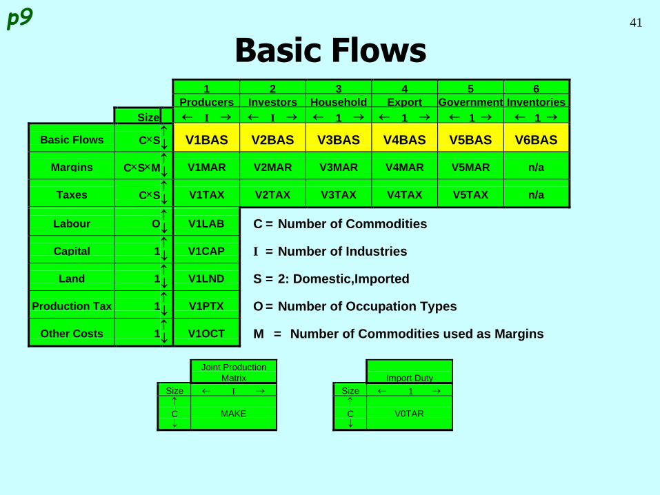
41
Basic Flows1 2 3 4 5 6
Producers Investors Household Export Government Inventories
Size I I 1 1 1 1
Basic Flows CS
V1BAS V2BAS V3BAS V4BAS V5BAS V6BAS
Margins CSM
V1MAR V2MAR V3MAR V4MAR V5MAR n/a
Taxes CS
V1TAX V2TAX V3TAX V4TAX V5TAX n/a
Labour O
V1LAB C = Number of Commodities
Capital 1
V1CAP I = Number of Industries
Land 1
V1LND S = 2: Domestic,Imported
Production Tax 1
V1PTX O = Number of Occupation Types
Other Costs 1
V1OCT M = Number of Commodities used as Margins
Joint Production
Matrix Import Duty
Size I Size 1
C
MAKE
C
V0TAR
p9
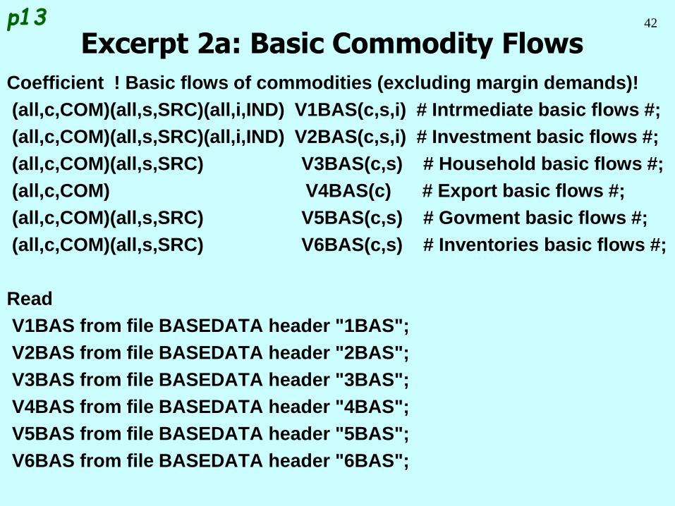
42
Excerpt 2a: Basic Commodity Flows
Coefficient ! Basic flows of commodities (excluding margin demands)!
(all,c,COM)(all,s,SRC)(all,i,IND) V1BAS(c,s,i) # Intrmediate basic flows #;
(all,c,COM)(all,s,SRC)(all,i,IND) V2BAS(c,s,i) # Investment basic flows #;
(all,c,COM)(all,s,SRC) V3BAS(c,s) # Household basic flows #;
(all,c,COM) V4BAS(c) # Export basic flows #;
(all,c,COM)(all,s,SRC) V5BAS(c,s) # Govment basic flows #;
(all,c,COM)(all,s,SRC) V6BAS(c,s) # Inventories basic flows #;
Read
V1BAS from file BASEDATA header "1BAS";
V2BAS from file BASEDATA header "2BAS";
V3BAS from file BASEDATA header "3BAS";
V4BAS from file BASEDATA header "4BAS";
V5BAS from file BASEDATA header "5BAS";
V6BAS from file BASEDATA header "6BAS";
p13
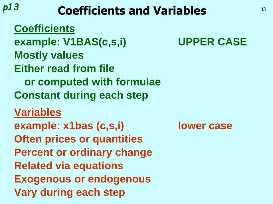
43Coefficients and Variables
Coefficients
example: V1BAS(c,s,i) UPPER CASE
Mostly values
Either read from file
or computed with formulae
Constant during each step
Variables
example: x1bas (c,s,i) lower case
Often prices or quantities
Percent or ordinary change
Related via equations
Exogenous or endogenous
Vary during each step
p13
44
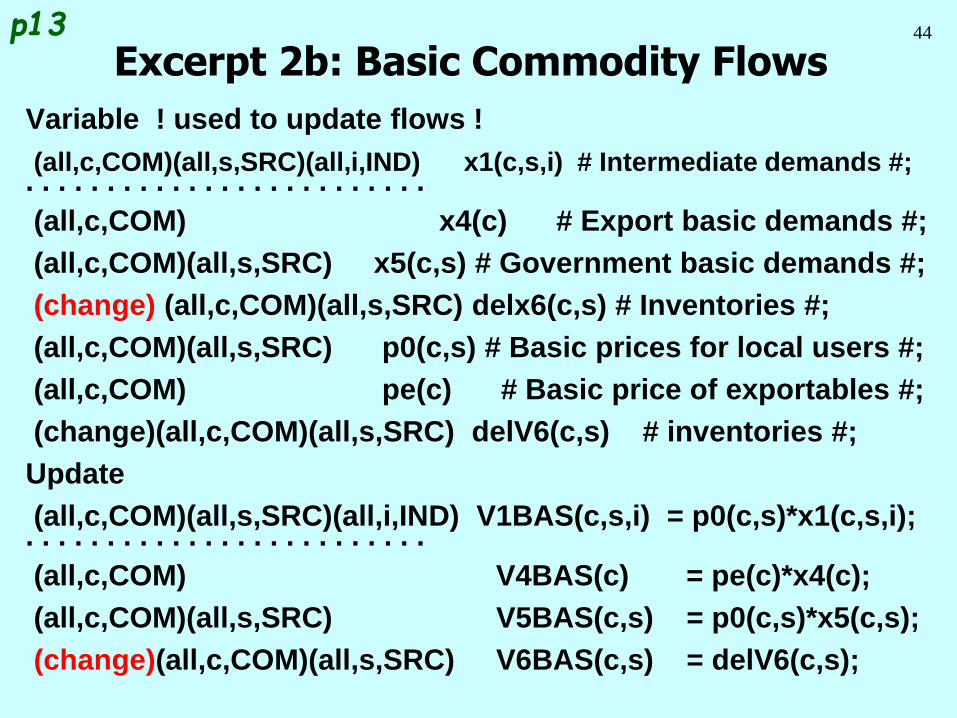
Excerpt 2b: Basic Commodity Flows
Variable ! used to update flows !
(all,c,COM)(all,s,SRC)(all,i,IND) x1(c,s,i) # Intermediate demands #;. . . . . . . . . . . . . . . . . . . . . . . . .
(all,c,COM) x4(c) # Export basic demands #;
(all,c,COM)(all,s,SRC) x5(c,s) # Government basic demands #;
(change) (all,c,COM)(all,s,SRC) delx6(c,s) # Inventories #;
(all,c,COM)(all,s,SRC) p0(c,s) # Basic prices for local users #;
(all,c,COM) pe(c) # Basic price of exportables #;
(change)(all,c,COM)(all,s,SRC) delV6(c,s) # inventories #;
Update
(all,c,COM)(all,s,SRC)(all,i,IND) V1BAS(c,s,i) = p0(c,s)*x1(c,s,i);. . . . . . . . . . . . . . . . . . . . . . . . .
(all,c,COM) V4BAS(c) = pe(c)*x4(c);
(all,c,COM)(all,s,SRC) V5BAS(c,s) = p0(c,s)*x5(c,s);
(change)(all,c,COM)(all,s,SRC) V6BAS(c,s) = delV6(c,s);
p13
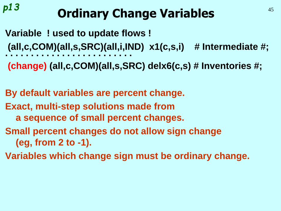
45Ordinary Change Variables
Variable ! used to update flows !
(all,c,COM)(all,s,SRC)(all,i,IND) x1(c,s,i) # Intermediate #;. . . . . . . . . . . . . . . . . . . . . . . . .
(change) (all,c,COM)(all,s,SRC) delx6(c,s) # Inventories #;
By default variables are percent change.
Exact, multi-step solutions made from
a sequence of small percent changes.
Small percent changes do not allow sign change
(eg, from 2 to -1).
Variables which change sign must be ordinary change.
p13
46
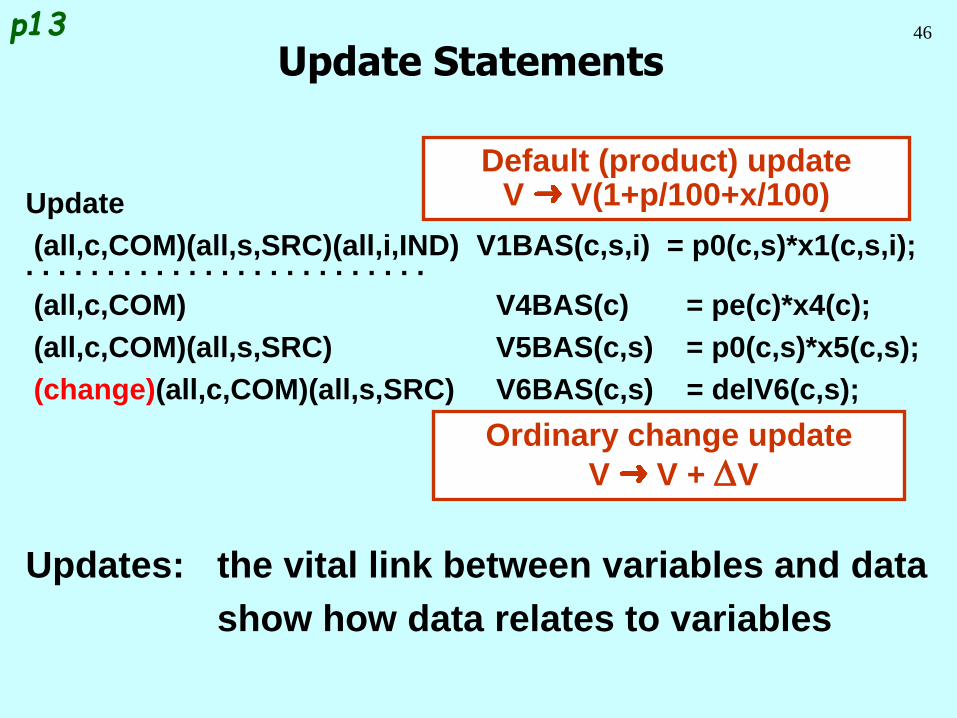
Update Statements
Update
(all,c,COM)(all,s,SRC)(all,i,IND) V1BAS(c,s,i) = p0(c,s)*x1(c,s,i);. . . . . . . . . . . . . . . . . . . . . . . . .
(all,c,COM) V4BAS(c) = pe(c)*x4(c);
(all,c,COM)(all,s,SRC) V5BAS(c,s) = p0(c,s)*x5(c,s);
(change)(all,c,COM)(all,s,SRC) V6BAS(c,s) = delV6(c,s);
Updates: the vital link between variables and data
show how data relates to variables
p13
Default (product) updateV V(1+p/100+x/100)
Ordinary change update
V V + DV
47
Margins1 2 3 4 5 6
Producers Investors Household Export Government Inventories
Size I I 1 1 1 1
Basic Flows CS
V1BAS V2BAS V3BAS V4BAS V5BAS V6BAS
Margins CSM
V1MAR V2MAR V3MAR V4MAR V5MAR n/a
Taxes CS
V1TAX V2TAX V3TAX V4TAX V5TAX n/a
Labour O
V1LAB C = Number of Commodities
Capital 1
V1CAP I = Number of Industries
Land 1
V1LND S = 2: Domestic,Imported
Production Tax 1
V1PTX O = Number of Occupation Types
Other Costs 1
V1OCT M = Number of Commodities used as Margins
Joint Production
Matrix Import Duty
Size I Size 1
C
MAKE
C
V0TAR
p9
48
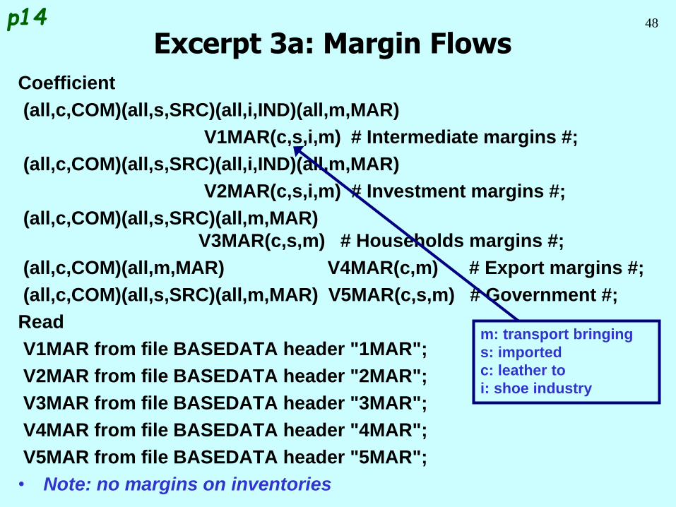
Coefficient
(all,c,COM)(all,s,SRC)(all,i,IND)(all,m,MAR)
V1MAR(c,s,i,m) # Intermediate margins #;
(all,c,COM)(all,s,SRC)(all,i,IND)(all,m,MAR)
V2MAR(c,s,i,m) # Investment margins #;
(all,c,COM)(all,s,SRC)(all,m,MAR)
V3MAR(c,s,m) # Households margins #;
(all,c,COM)(all,m,MAR) V4MAR(c,m) # Export margins #;
(all,c,COM)(all,s,SRC)(all,m,MAR) V5MAR(c,s,m) # Government #;
Read
V1MAR from file BASEDATA header "1MAR";
V2MAR from file BASEDATA header "2MAR";
V3MAR from file BASEDATA header "3MAR";
V4MAR from file BASEDATA header "4MAR";
V5MAR from file BASEDATA header "5MAR";
• Note: no margins on inventories
Excerpt 3a: Margin Flows
m: transport bringing
s: imported
c: leather to
i: shoe industry
p14
49
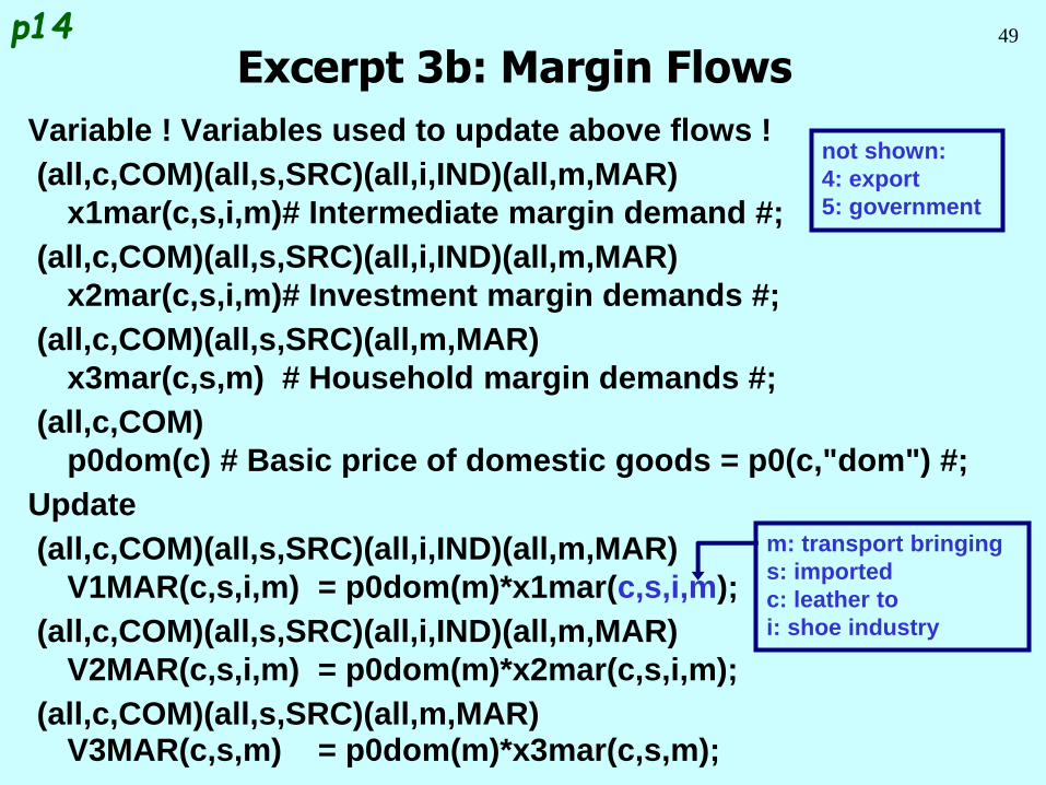
Variable ! Variables used to update above flows !
(all,c,COM)(all,s,SRC)(all,i,IND)(all,m,MAR)
x1mar(c,s,i,m)# Intermediate margin demand #;
(all,c,COM)(all,s,SRC)(all,i,IND)(all,m,MAR)
x2mar(c,s,i,m)# Investment margin demands #;
(all,c,COM)(all,s,SRC)(all,m,MAR)
x3mar(c,s,m) # Household margin demands #;
(all,c,COM)
p0dom(c) # Basic price of domestic goods = p0(c,"dom") #;
Update
(all,c,COM)(all,s,SRC)(all,i,IND)(all,m,MAR)
V1MAR(c,s,i,m) = p0dom(m)*x1mar(c,s,i,m);
(all,c,COM)(all,s,SRC)(all,i,IND)(all,m,MAR)
V2MAR(c,s,i,m) = p0dom(m)*x2mar(c,s,i,m);
(all,c,COM)(all,s,SRC)(all,m,MAR)V3MAR(c,s,m) = p0dom(m)*x3mar(c,s,m);
Excerpt 3b: Margin Flows
m: transport bringing
s: imported
c: leather to
i: shoe industry
p14
not shown:
4: export
5: government

50
Commodity Taxes1 2 3 4 5 6
Producers Investors Household Export Government Inventories
Size I I 1 1 1 1
Basic Flows CS
V1BAS V2BAS V3BAS V4BAS V5BAS V6BAS
Margins CSM
V1MAR V2MAR V3MAR V4MAR V5MAR n/a
Taxes CS
V1TAX V2TAX V3TAX V4TAX V5TAX n/a
Labour O
V1LAB C = Number of Commodities
Capital 1
V1CAP I = Number of Industries
Land 1
V1LND S = 2: Domestic,Imported
Production Tax 1
V1PTX O = Number of Occupation Types
Other Costs 1
V1OCT M = Number of Commodities used as Margins
Joint Production
Matrix Import Duty
Size I Size 1
C
MAKE
C
V0TAR
p9
51
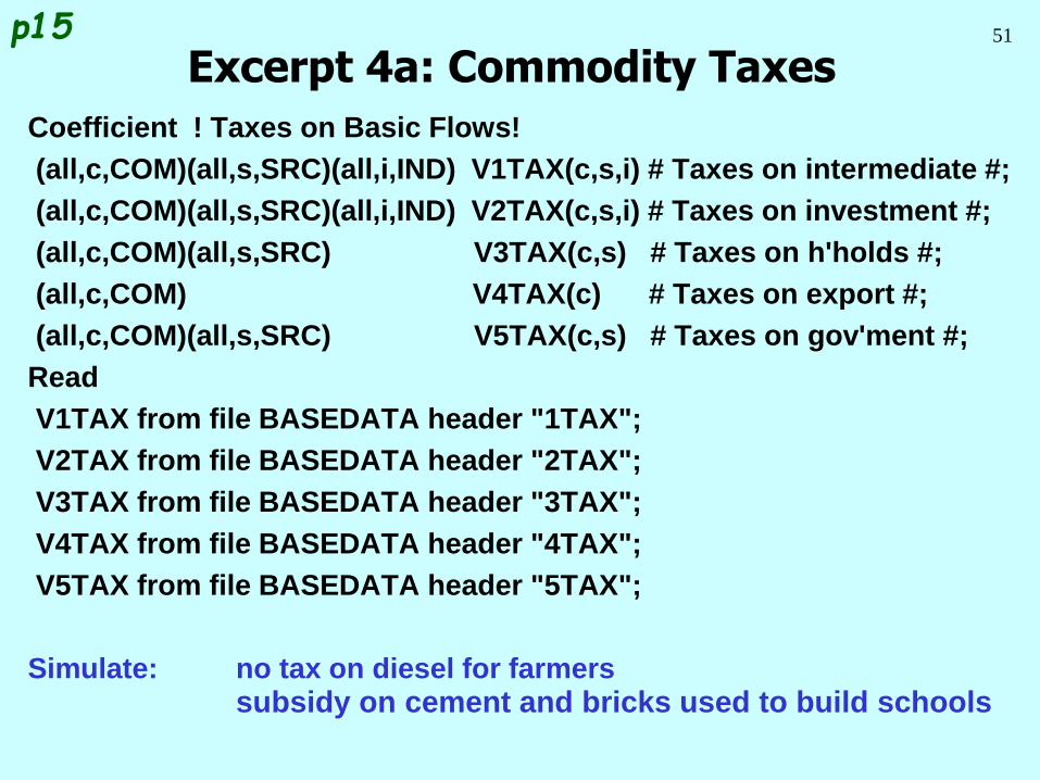
Coefficient ! Taxes on Basic Flows!
(all,c,COM)(all,s,SRC)(all,i,IND) V1TAX(c,s,i) # Taxes on intermediate #;
(all,c,COM)(all,s,SRC)(all,i,IND) V2TAX(c,s,i) # Taxes on investment #;
(all,c,COM)(all,s,SRC) V3TAX(c,s) # Taxes on h'holds #;
(all,c,COM) V4TAX(c) # Taxes on export #;
(all,c,COM)(all,s,SRC) V5TAX(c,s) # Taxes on gov'ment #;
Read
V1TAX from file BASEDATA header "1TAX";
V2TAX from file BASEDATA header "2TAX";
V3TAX from file BASEDATA header "3TAX";
V4TAX from file BASEDATA header "4TAX";
V5TAX from file BASEDATA header "5TAX";
Simulate: no tax on diesel for farmers
subsidy on cement and bricks used to build schools
Excerpt 4a: Commodity Taxesp15
52
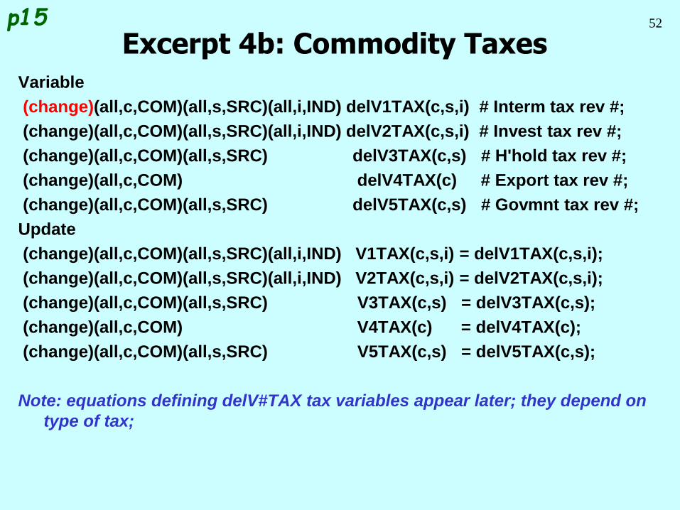
Variable
(change)(all,c,COM)(all,s,SRC)(all,i,IND) delV1TAX(c,s,i) # Interm tax rev #;
(change)(all,c,COM)(all,s,SRC)(all,i,IND) delV2TAX(c,s,i) # Invest tax rev #;
(change)(all,c,COM)(all,s,SRC) delV3TAX(c,s) # H'hold tax rev #;
(change)(all,c,COM) delV4TAX(c) # Export tax rev #;
(change)(all,c,COM)(all,s,SRC) delV5TAX(c,s) # Govmnt tax rev #;
Update
(change)(all,c,COM)(all,s,SRC)(all,i,IND) V1TAX(c,s,i) = delV1TAX(c,s,i);
(change)(all,c,COM)(all,s,SRC)(all,i,IND) V2TAX(c,s,i) = delV2TAX(c,s,i);
(change)(all,c,COM)(all,s,SRC) V3TAX(c,s) = delV3TAX(c,s);
(change)(all,c,COM) V4TAX(c) = delV4TAX(c);
(change)(all,c,COM)(all,s,SRC) V5TAX(c,s) = delV5TAX(c,s);
Note: equations defining delV#TAX tax variables appear later; they depend on
type of tax;
Excerpt 4b: Commodity Taxesp15
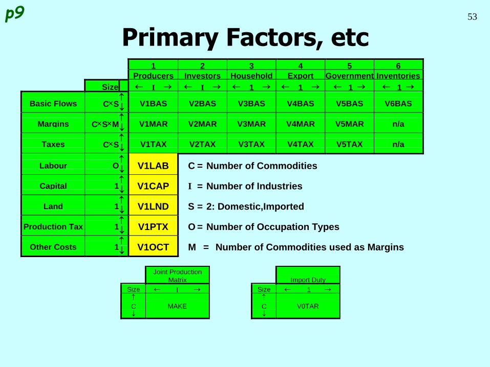
53
Primary Factors, etc1 2 3 4 5 6
Producers Investors Household Export Government Inventories
Size I I 1 1 1 1
Basic Flows CS
V1BAS V2BAS V3BAS V4BAS V5BAS V6BAS
Margins CSM
V1MAR V2MAR V3MAR V4MAR V5MAR n/a
Taxes CS
V1TAX V2TAX V3TAX V4TAX V5TAX n/a
Labour O
V1LAB C = Number of Commodities
Capital 1
V1CAP I = Number of Industries
Land 1
V1LND S = 2: Domestic,Imported
Production Tax 1
V1PTX O = Number of Occupation Types
Other Costs 1
V1OCT M = Number of Commodities used as Margins
Joint Production
Matrix Import Duty
Size I Size 1
C
MAKE
C
V0TAR
p9
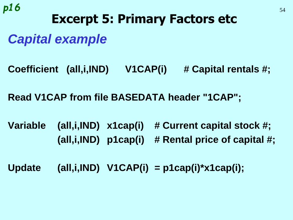
54
Capital example
Coefficient (all,i,IND) V1CAP(i) # Capital rentals #;
Read V1CAP from file BASEDATA header "1CAP";
Variable (all,i,IND) x1cap(i) # Current capital stock #;
(all,i,IND) p1cap(i) # Rental price of capital #;
Update (all,i,IND) V1CAP(i) = p1cap(i)*x1cap(i);
Excerpt 5: Primary Factors etcp16
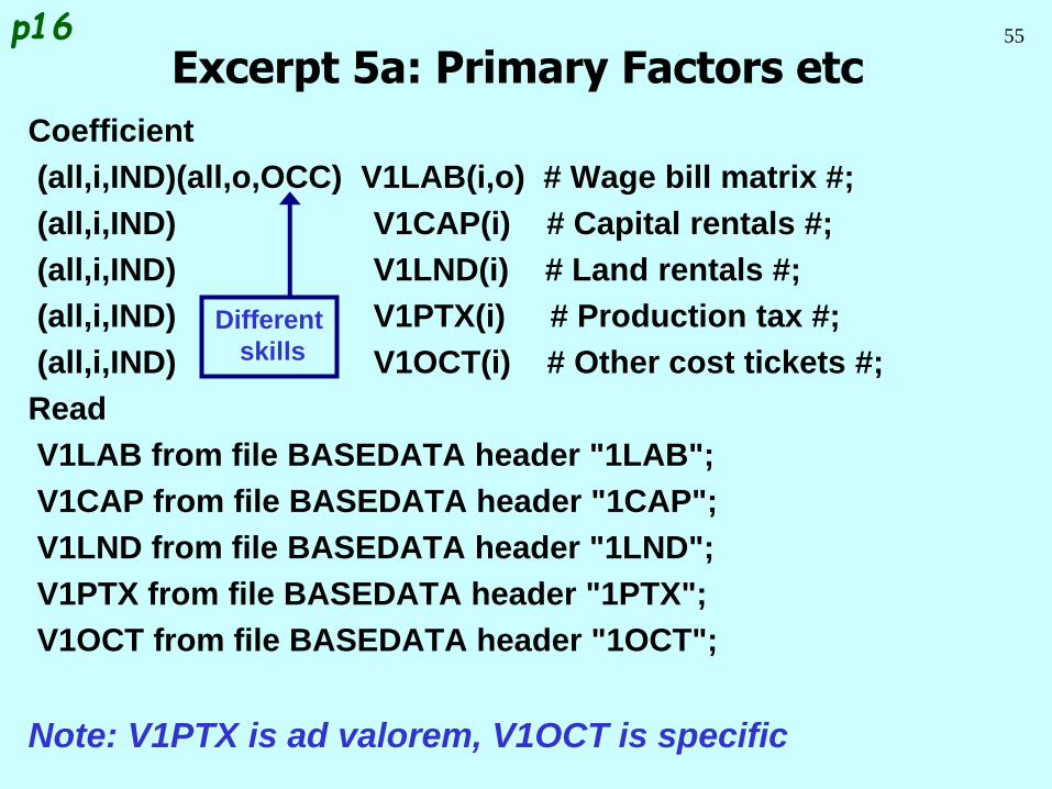
55
Coefficient
(all,i,IND)(all,o,OCC) V1LAB(i,o) # Wage bill matrix #;
(all,i,IND) V1CAP(i) # Capital rentals #;
(all,i,IND) V1LND(i) # Land rentals #;
(all,i,IND) V1PTX(i) # Production tax #;
(all,i,IND) V1OCT(i) # Other cost tickets #;
Read
V1LAB from file BASEDATA header "1LAB";
V1CAP from file BASEDATA header "1CAP";
V1LND from file BASEDATA header "1LND";
V1PTX from file BASEDATA header "1PTX";
V1OCT from file BASEDATA header "1OCT";
Note: V1PTX is ad valorem, V1OCT is specific
Excerpt 5a: Primary Factors etc
Different
skills
p16
56
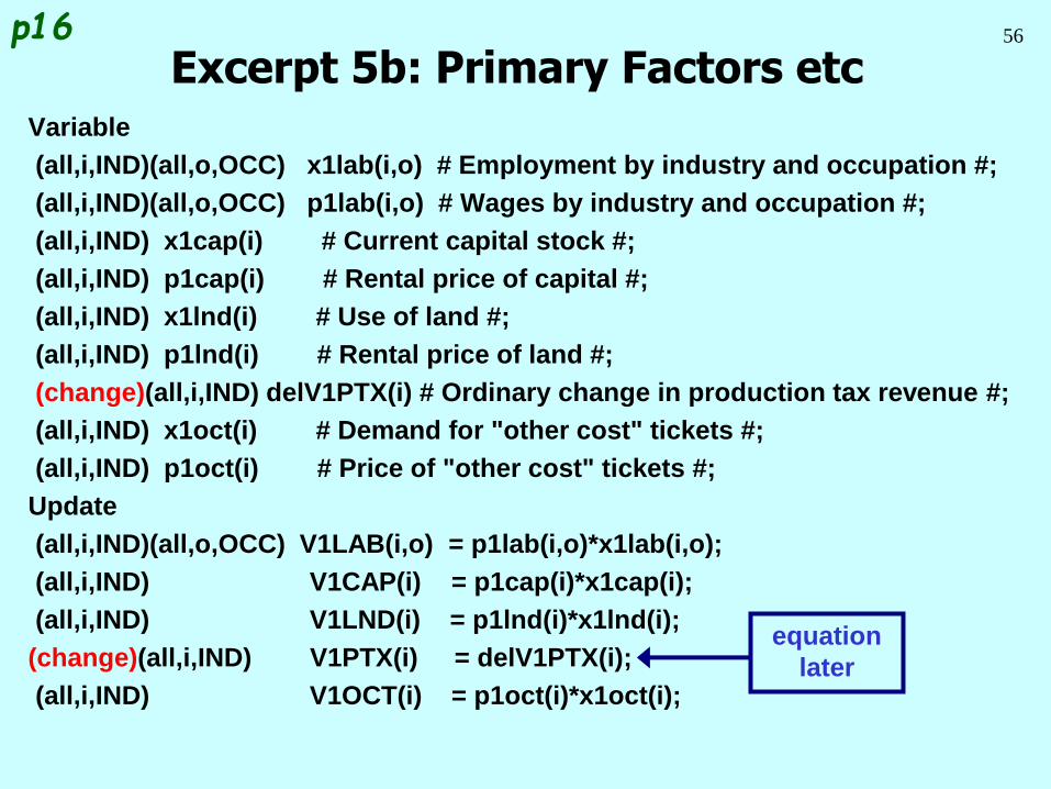
Variable
(all,i,IND)(all,o,OCC) x1lab(i,o) # Employment by industry and occupation #;
(all,i,IND)(all,o,OCC) p1lab(i,o) # Wages by industry and occupation #;
(all,i,IND) x1cap(i) # Current capital stock #;
(all,i,IND) p1cap(i) # Rental price of capital #;
(all,i,IND) x1lnd(i) # Use of land #;
(all,i,IND) p1lnd(i) # Rental price of land #;
(change)(all,i,IND) delV1PTX(i) # Ordinary change in production tax revenue #;
(all,i,IND) x1oct(i) # Demand for "other cost" tickets #;
(all,i,IND) p1oct(i) # Price of "other cost" tickets #;
Update
(all,i,IND)(all,o,OCC) V1LAB(i,o) = p1lab(i,o)*x1lab(i,o);
(all,i,IND) V1CAP(i) = p1cap(i)*x1cap(i);
(all,i,IND) V1LND(i) = p1lnd(i)*x1lnd(i);
(change)(all,i,IND) V1PTX(i) = delV1PTX(i);
(all,i,IND) V1OCT(i) = p1oct(i)*x1oct(i);
Excerpt 5b: Primary Factors etcp16
equation
later
57
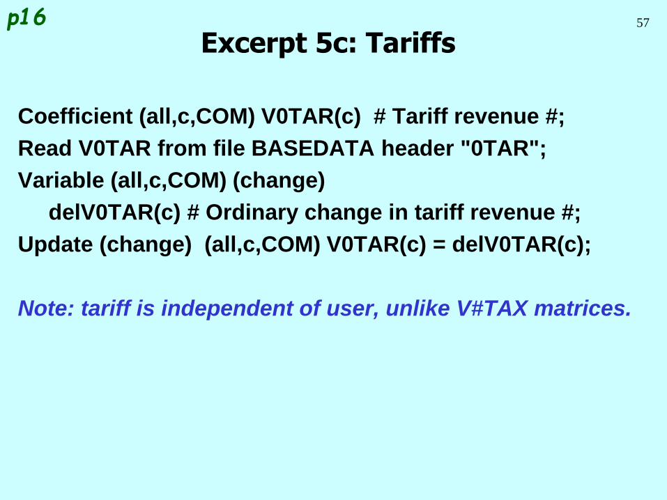
Coefficient (all,c,COM) V0TAR(c) # Tariff revenue #;
Read V0TAR from file BASEDATA header "0TAR";
Variable (all,c,COM) (change)
delV0TAR(c) # Ordinary change in tariff revenue #;
Update (change) (all,c,COM) V0TAR(c) = delV0TAR(c);
Note: tariff is independent of user, unlike V#TAX matrices.
Excerpt 5c: Tariffsp16
58
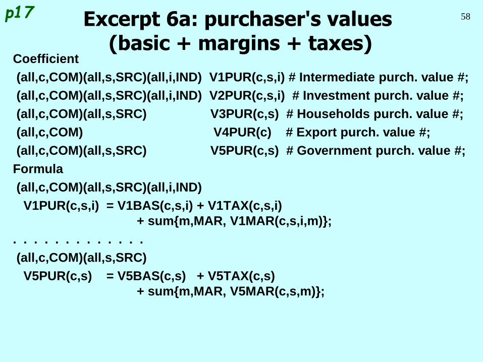
Coefficient
(all,c,COM)(all,s,SRC)(all,i,IND) V1PUR(c,s,i) # Intermediate purch. value #;
(all,c,COM)(all,s,SRC)(all,i,IND) V2PUR(c,s,i) # Investment purch. value #;
(all,c,COM)(all,s,SRC) V3PUR(c,s) # Households purch. value #;
(all,c,COM) V4PUR(c) # Export purch. value #;
(all,c,COM)(all,s,SRC) V5PUR(c,s) # Government purch. value #;
Formula
(all,c,COM)(all,s,SRC)(all,i,IND)
V1PUR(c,s,i) = V1BAS(c,s,i) + V1TAX(c,s,i)
+ sum{m,MAR, V1MAR(c,s,i,m)};
. . . . . . . . . . . . .
(all,c,COM)(all,s,SRC)
V5PUR(c,s) = V5BAS(c,s) + V5TAX(c,s)
+ sum{m,MAR, V5MAR(c,s,m)};
Excerpt 6a: purchaser's values(basic + margins + taxes)
p17
59
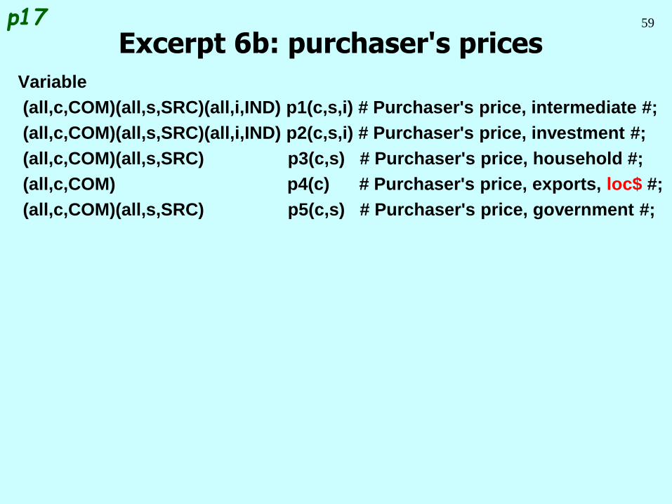
Variable
(all,c,COM)(all,s,SRC)(all,i,IND) p1(c,s,i) # Purchaser's price, intermediate #;
(all,c,COM)(all,s,SRC)(all,i,IND) p2(c,s,i) # Purchaser's price, investment #;
(all,c,COM)(all,s,SRC) p3(c,s) # Purchaser's price, household #;
(all,c,COM) p4(c) # Purchaser's price, exports, loc$ #;
(all,c,COM)(all,s,SRC) p5(c,s) # Purchaser's price, government #;
Excerpt 6b: purchaser's pricesp17
60
Progress so far . . .
Introduction Inventory demands
Database structure Margin demands
Solution method Market clearing
TABLO language Price equations
Production: input decisions Aggregates and indices
Production: output decisions Investment allocation
Investment: input decisions Labour market
Household demands Decompositions
Export demands Closure
Government demands Regional extension
61
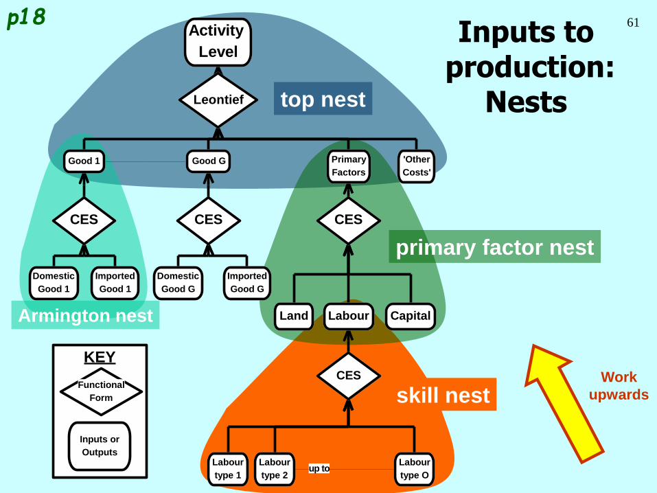
Inputs toproduction:
Nests
p18
skill nest
primary factor nest
top nest
Armington nest
KEY
Inputs or
Outputs
Functional
Form
CES
CES
Leontief
CESCES
up toLabour
type O
Labour
type 2
Labour
type 1
CapitalLabourLand
'Other
Costs'
Primary
Factors
Imported
Good G
Domestic
Good G
Imported
Good 1
Domestic
Good 1
Good GGood 1
Activity
Level
Work
upwards
62Nested Structure of production
In each industry: Output = function of inputs:
output = F(inputs) = F(Labour, Capital, Land, dom goods, imp goods)
Separability assumptions simplify the production structure:
output = F(primary factor composite, composite goods)
where:
primary factor composite = CES(Labour, Capital. Land)
labour = CES(Various skill grades)
composite good (i) = CES(domestic good (i), imported good (i))
All industries share common production structure.
BUT: Input proportions and behavioural parameters vary.
Nesting is like staged decisions:
First decide how much leather to use—based on output.
Then decide import/domestic proportions, depending on the
relative prices of local and foreign leather.
Each nest requires 2 or 3 equations.
63
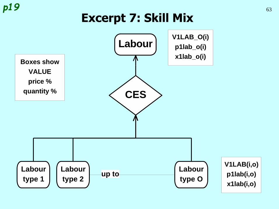
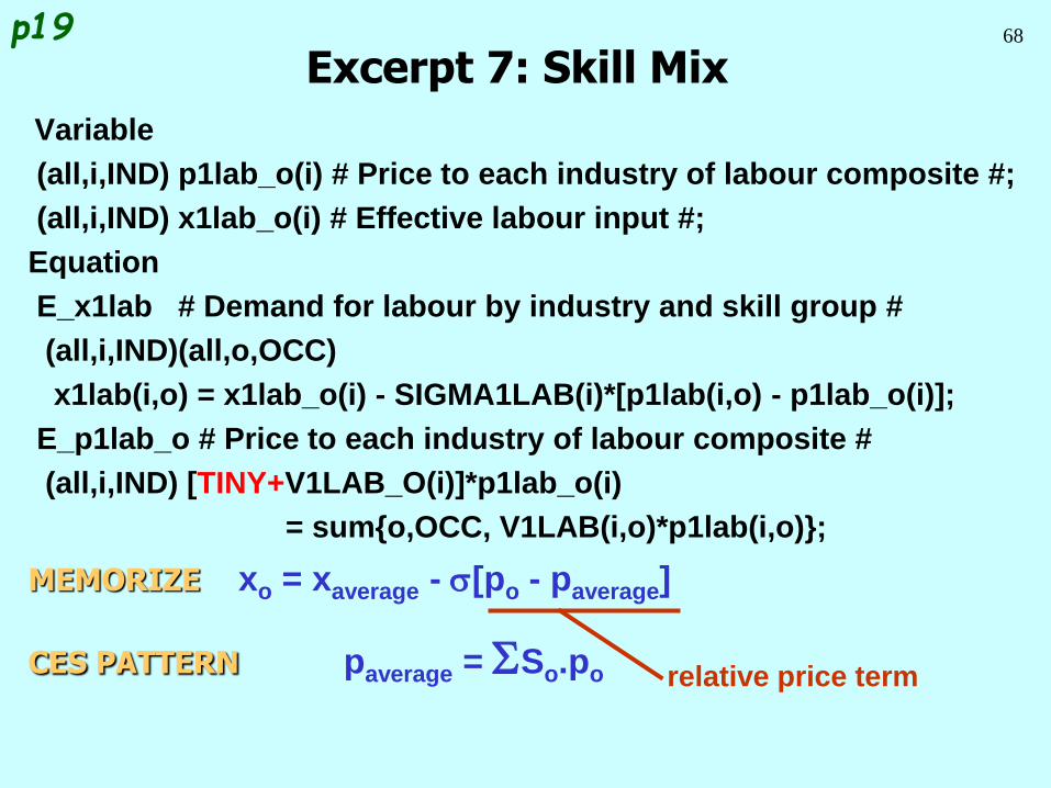
Excerpt 7: Skill Mix
CES
up toLabour
type O
Labour
type 2
Labour
type 1
Labour
V1LAB(i,o)
p1lab(i,o)
x1lab(i,o)
V1LAB_O(i)
p1lab_o(i)
x1lab_o(i)Boxes show
VALUE
price %
quantity %
p19
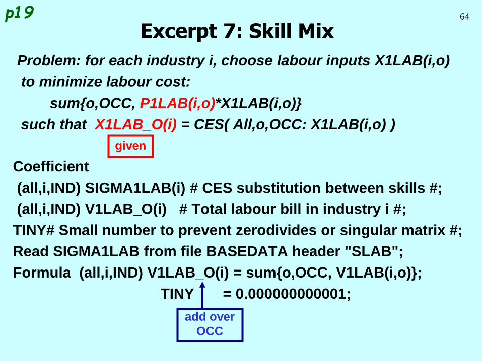
64
Problem: for each industry i, choose labour inputs X1LAB(i,o)
to minimize labour cost:
sum{o,OCC, P1LAB(i,o)*X1LAB(i,o)}
such that X1LAB_O(i) = CES( All,o,OCC: X1LAB(i,o) )
Coefficient
(all,i,IND) SIGMA1LAB(i) # CES substitution between skills #;
(all,i,IND) V1LAB_O(i) # Total labour bill in industry i #;
TINY# Small number to prevent zerodivides or singular matrix #;
Read SIGMA1LAB from file BASEDATA header "SLAB";
Formula (all,i,IND) V1LAB_O(i) = sum{o,OCC, V1LAB(i,o)};
TINY = 0.000000000001;
Excerpt 7: Skill Mixp19
add over
OCC
given
65
X=15
X=10
SkilledXs
Cost=$9
A
B
C
R
Cost=$6UnSkilled
Xu
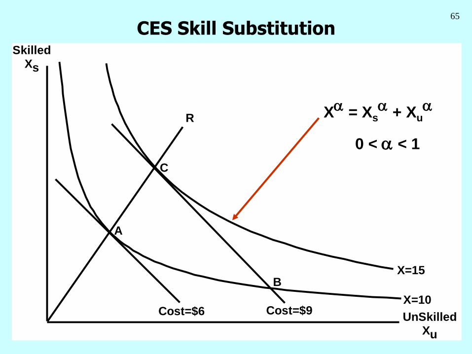
CES Skill Substitution
Xa = Xsa + Xu
a
0 < a < 1
66
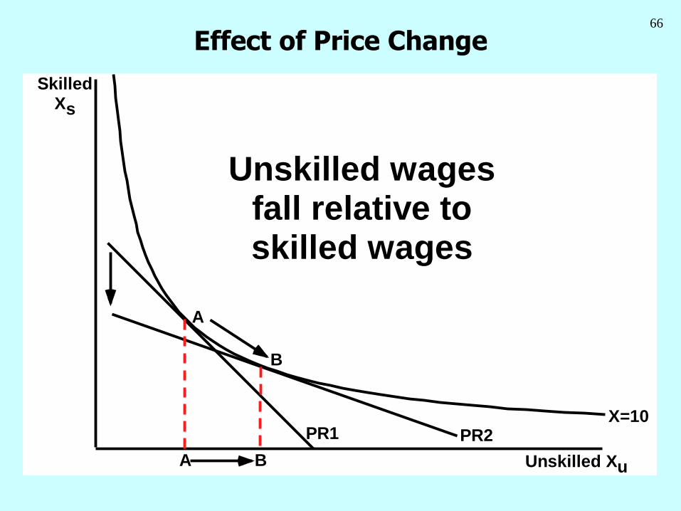
Effect of Price Change
•X=10
SkilledXs
Unskilled Xu
PR1
A
B
PR2
Unskilled wagesfall relative toskilled wages
A B
67
Deriving the CES demand equations
See ORANI-G document Appendix A
68
Variable
(all,i,IND) p1lab_o(i) # Price to each industry of labour composite #;
(all,i,IND) x1lab_o(i) # Effective labour input #;
Equation
E_x1lab # Demand for labour by industry and skill group #
(all,i,IND)(all,o,OCC)
x1lab(i,o) = x1lab_o(i) - SIGMA1LAB(i)*[p1lab(i,o) - p1lab_o(i)];
E_p1lab_o # Price to each industry of labour composite #
(all,i,IND) [TINY+V1LAB_O(i)]*p1lab_o(i)
= sum{o,OCC, V1LAB(i,o)*p1lab(i,o)};
MEMORIZE xo = xaverage - s[po - paverage]
CES PATTERN paverage = SSo.po
Excerpt 7: Skill Mixp19
relative price term
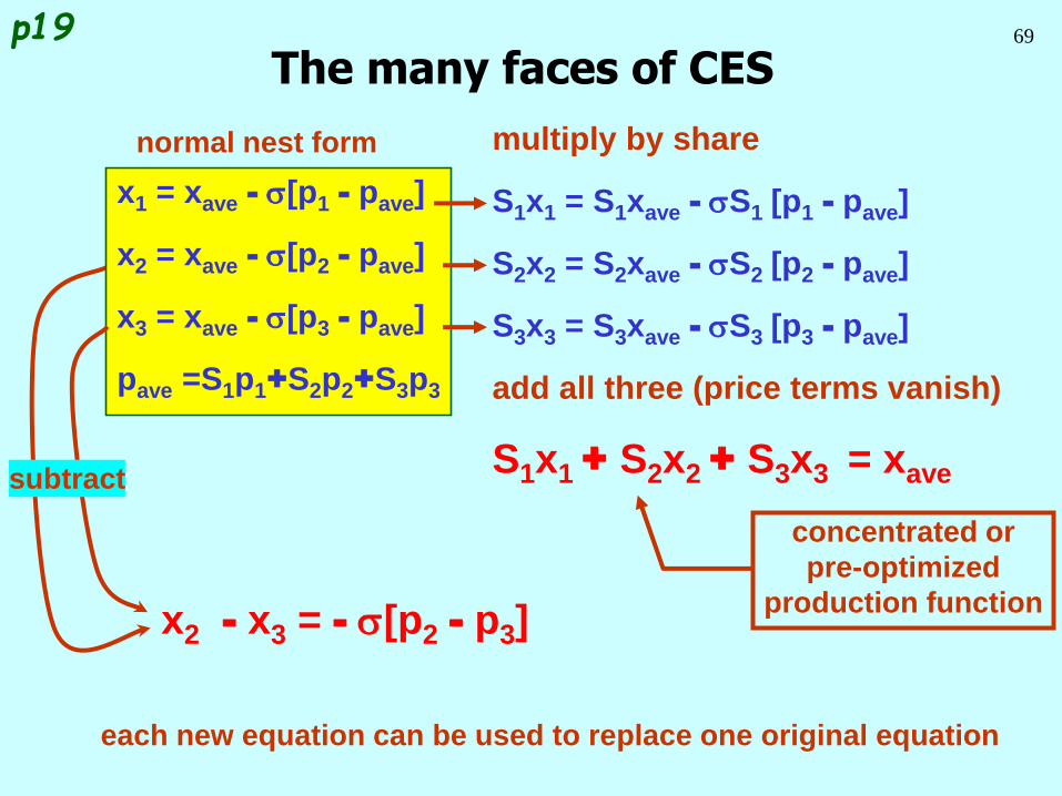
69
x2 - x3 = - s[p2 - p3]
The many faces of CESp19
multiply by share
S1x1 = S1xave - sS1 [p1 - pave]
S2x2 = S2xave - sS2 [p2 - pave]
S3x3 = S3xave - sS3 [p3 - pave]
add all three (price terms vanish)
S1x1 + S2x2 + S3x3 = xave
x1 = xave - s[p1 - pave]
x2 = xave - s[p2 - pave]
x3 = xave - s[p3 - pave]
pave =S1p1+S2p2+S3p3
subtract
concentrated or
pre-optimized
production function
each new equation can be used to replace one original equation
normal nest form
70
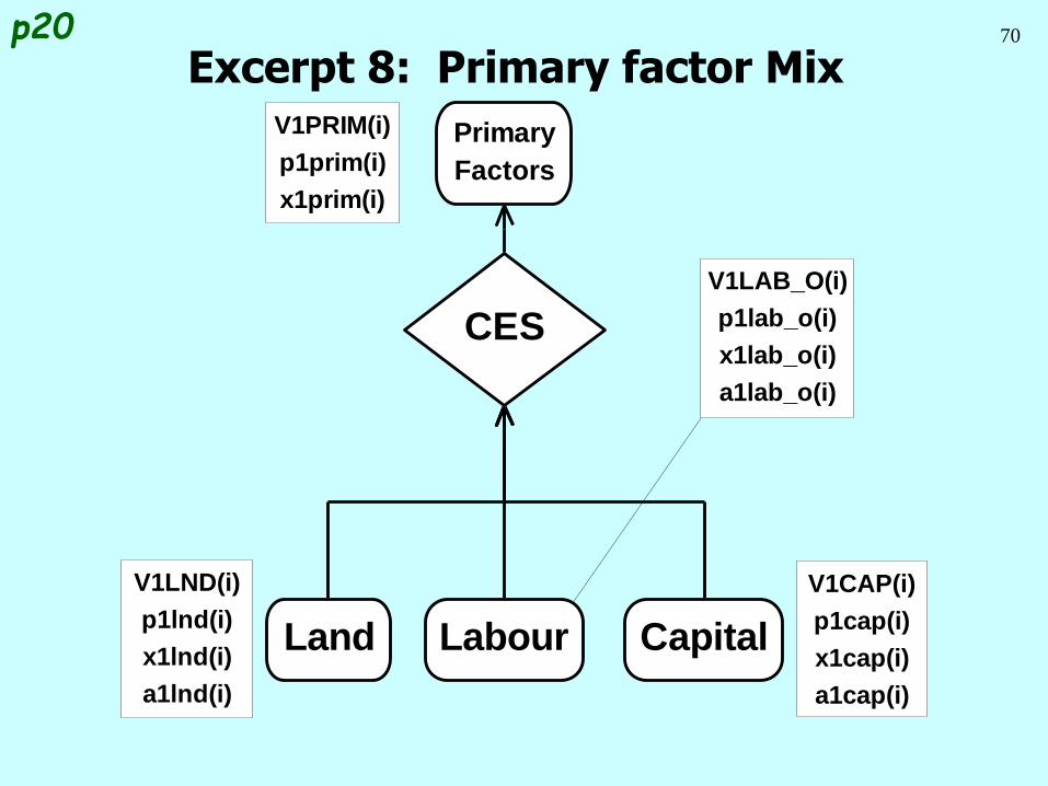
Excerpt 8: Primary factor Mix
CES
CapitalLabourLand
Primary
Factors
V1CAP(i)
p1cap(i)
x1cap(i)
a1cap(i)
V1PRIM(i)
p1prim(i)
x1prim(i)
V1LAB_O(i)
p1lab_o(i)
x1lab_o(i)
a1lab_o(i)
V1LND(i)
p1lnd(i)
x1lnd(i)
a1lnd(i)
p20
71
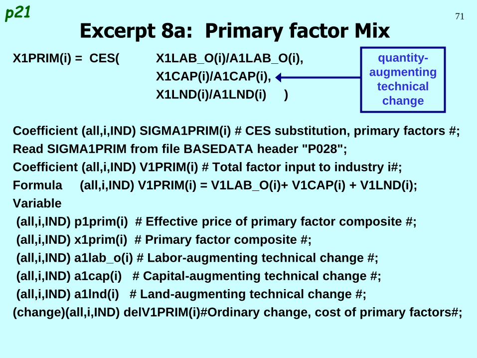
X1PRIM(i) = CES( X1LAB_O(i)/A1LAB_O(i),
X1CAP(i)/A1CAP(i),
X1LND(i)/A1LND(i) )
Coefficient (all,i,IND) SIGMA1PRIM(i) # CES substitution, primary factors #;
Read SIGMA1PRIM from file BASEDATA header "P028";
Coefficient (all,i,IND) V1PRIM(i) # Total factor input to industry i#;
Formula (all,i,IND) V1PRIM(i) = V1LAB_O(i)+ V1CAP(i) + V1LND(i);
Variable
(all,i,IND) p1prim(i) # Effective price of primary factor composite #;
(all,i,IND) x1prim(i) # Primary factor composite #;
(all,i,IND) a1lab_o(i) # Labor-augmenting technical change #;
(all,i,IND) a1cap(i) # Capital-augmenting technical change #;
(all,i,IND) a1lnd(i) # Land-augmenting technical change #;
(change)(all,i,IND) delV1PRIM(i)#Ordinary change, cost of primary factors#;
Excerpt 8a: Primary factor Mixp21
quantity-
augmenting
technical
change
72
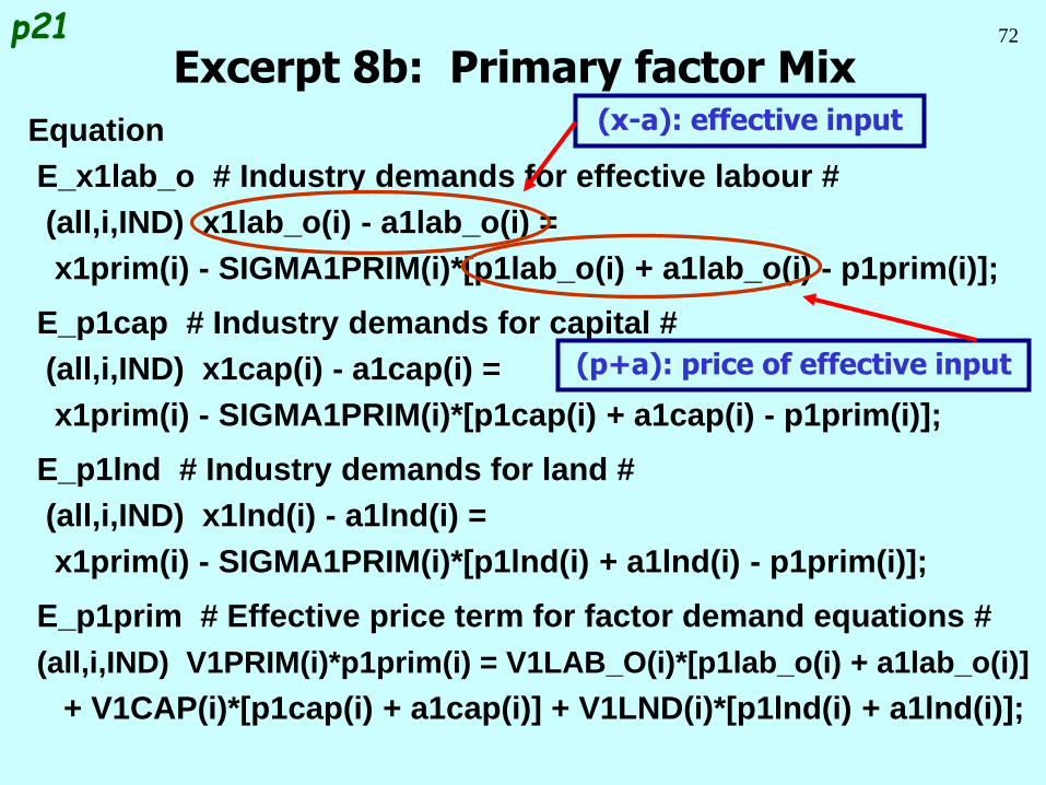
Equation
E_x1lab_o # Industry demands for effective labour #
(all,i,IND) x1lab_o(i) - a1lab_o(i) =
x1prim(i) - SIGMA1PRIM(i)*[p1lab_o(i) + a1lab_o(i) - p1prim(i)];
E_p1cap # Industry demands for capital #
(all,i,IND) x1cap(i) - a1cap(i) =
x1prim(i) - SIGMA1PRIM(i)*[p1cap(i) + a1cap(i) - p1prim(i)];
E_p1lnd # Industry demands for land #
(all,i,IND) x1lnd(i) - a1lnd(i) =
x1prim(i) - SIGMA1PRIM(i)*[p1lnd(i) + a1lnd(i) - p1prim(i)];
E_p1prim # Effective price term for factor demand equations #
(all,i,IND) V1PRIM(i)*p1prim(i) = V1LAB_O(i)*[p1lab_o(i) + a1lab_o(i)]
+ V1CAP(i)*[p1cap(i) + a1cap(i)] + V1LND(i)*[p1lnd(i) + a1lnd(i)];
Excerpt 8b: Primary factor Mix(x-a): effective input
(p+a): price of effective input
p21
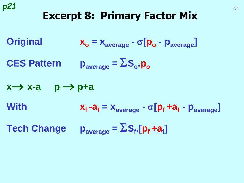
73
Original xo = xaverage - s[po - paverage]
CES Pattern paverage = SSo.po
x x-a p p+a
With xf -af = xaverage - s[pf +af - paverage]
Tech Change paverage = SSf.[pf +af]
Excerpt 8: Primary Factor Mixp21
74
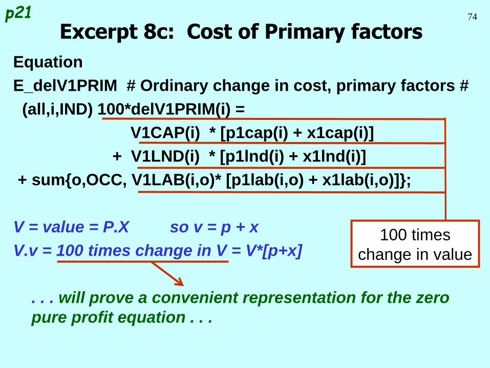
Equation
E_delV1PRIM # Ordinary change in cost, primary factors #
(all,i,IND) 100*delV1PRIM(i) =
V1CAP(i) * [p1cap(i) + x1cap(i)]
+ V1LND(i) * [p1lnd(i) + x1lnd(i)]
+ sum{o,OCC, V1LAB(i,o)* [p1lab(i,o) + x1lab(i,o)]};
V = value = P.X so v = p + x
V.v = 100 times change in V = V*[p+x]
. . . will prove a convenient representation for the zero
pure profit equation . . .
Excerpt 8c: Cost of Primary factorsp21
100 times
change in value
75
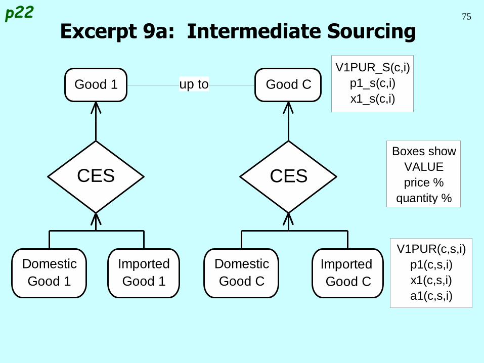
Excerpt 9a: Intermediate Sourcing
CESCES
up to
Imported
Good C
Domestic
Good C
Imported
Good 1
Domestic
Good 1
Good CGood 1
V1PUR_S(c,i)
p1_s(c,i)
x1_s(c,i)
V1PUR(c,s,i)
p1(c,s,i)
x1(c,s,i)
a1(c,s,i)
Boxes show
VALUE
price %
quantity %
p22
76
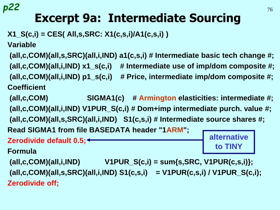
X1_S(c,i) = CES( All,s,SRC: X1(c,s,i)/A1(c,s,i) )
Variable
(all,c,COM)(all,s,SRC)(all,i,IND) a1(c,s,i) # Intermediate basic tech change #;
(all,c,COM)(all,i,IND) x1_s(c,i) # Intermediate use of imp/dom composite #;
(all,c,COM)(all,i,IND) p1_s(c,i) # Price, intermediate imp/dom composite #;
Coefficient
(all,c,COM) SIGMA1(c) # Armington elasticities: intermediate #;
(all,c,COM)(all,i,IND) V1PUR_S(c,i) # Dom+imp intermediate purch. value #;
(all,c,COM)(all,s,SRC)(all,i,IND) S1(c,s,i) # Intermediate source shares #;
Read SIGMA1 from file BASEDATA header "1ARM";
Zerodivide default 0.5;
Formula
(all,c,COM)(all,i,IND) V1PUR_S(c,i) = sum{s,SRC, V1PUR(c,s,i)};
(all,c,COM)(all,s,SRC)(all,i,IND) S1(c,s,i) = V1PUR(c,s,i) / V1PUR_S(c,i);
Zerodivide off;
Excerpt 9a: Intermediate Sourcingp22
alternative
to TINY
77
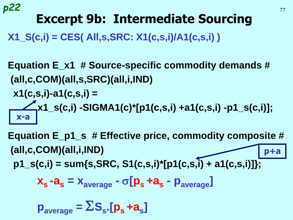
X1_S(c,i) = CES( All,s,SRC: X1(c,s,i)/A1(c,s,i) )
Equation E_x1 # Source-specific commodity demands #
(all,c,COM)(all,s,SRC)(all,i,IND)
x1(c,s,i)-a1(c,s,i) =
x1_s(c,i) -SIGMA1(c)*[p1(c,s,i) +a1(c,s,i) -p1_s(c,i)];
Equation E_p1_s # Effective price, commodity composite #
(all,c,COM)(all,i,IND)
p1_s(c,i) = sum{s,SRC, S1(c,s,i)*[p1(c,s,i) + a1(c,s,i)]};
xs -as = xaverage - s[ps +as - paverage]
paverage = SSs.[ps +as]
Excerpt 9b: Intermediate Sourcingp22
x-a
p+a
78
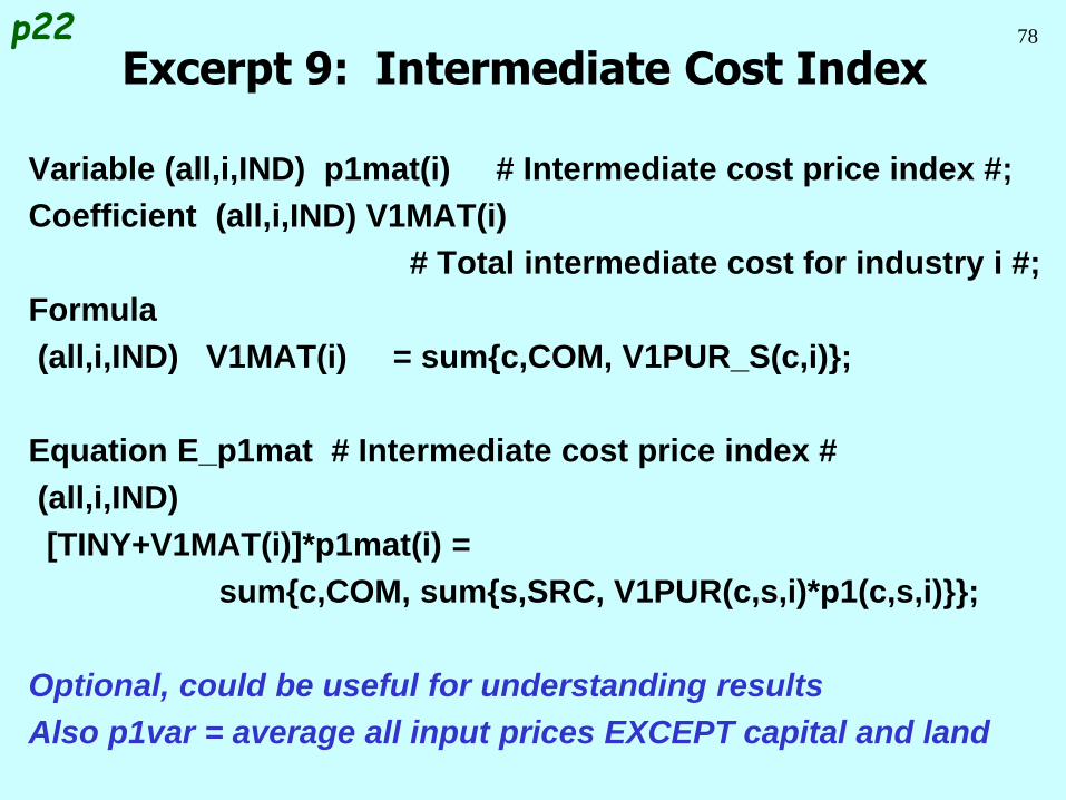
Variable (all,i,IND) p1mat(i) # Intermediate cost price index #;
Coefficient (all,i,IND) V1MAT(i)
# Total intermediate cost for industry i #;
Formula
(all,i,IND) V1MAT(i) = sum{c,COM, V1PUR_S(c,i)};
Equation E_p1mat # Intermediate cost price index #
(all,i,IND)
[TINY+V1MAT(i)]*p1mat(i) =
sum{c,COM, sum{s,SRC, V1PUR(c,s,i)*p1(c,s,i)}};
Optional, could be useful for understanding results
Also p1var = average all input prices EXCEPT capital and land
Excerpt 9: Intermediate Cost Indexp22
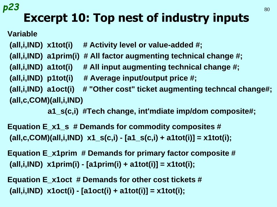
79
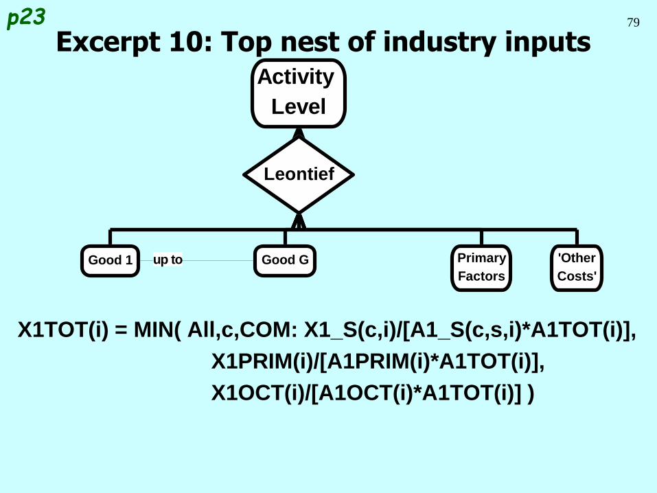
X1TOT(i) = MIN( All,c,COM: X1_S(c,i)/[A1_S(c,s,i)*A1TOT(i)],
X1PRIM(i)/[A1PRIM(i)*A1TOT(i)],
X1OCT(i)/[A1OCT(i)*A1TOT(i)] )
Excerpt 10: Top nest of industry inputs
Leontief
up to 'Other
Costs'
Primary
Factors
Good GGood 1
Activity
Level
p23
80
Variable
(all,i,IND) x1tot(i) # Activity level or value-added #;
(all,i,IND) a1prim(i) # All factor augmenting technical change #;
(all,i,IND) a1tot(i) # All input augmenting technical change #;
(all,i,IND) p1tot(i) # Average input/output price #;
(all,i,IND) a1oct(i) # "Other cost" ticket augmenting techncal change#;
(all,c,COM)(all,i,IND)
a1_s(c,i) #Tech change, int'mdiate imp/dom composite#;
Equation E_x1_s # Demands for commodity composites #
(all,c,COM)(all,i,IND) x1_s(c,i) - [a1_s(c,i) + a1tot(i)] = x1tot(i);
Equation E_x1prim # Demands for primary factor composite #
(all,i,IND) x1prim(i) - [a1prim(i) + a1tot(i)] = x1tot(i);
Equation E_x1oct # Demands for other cost tickets #
(all,i,IND) x1oct(i) - [a1oct(i) + a1tot(i)] = x1tot(i);
Excerpt 10: Top nest of industry inputsp23
81
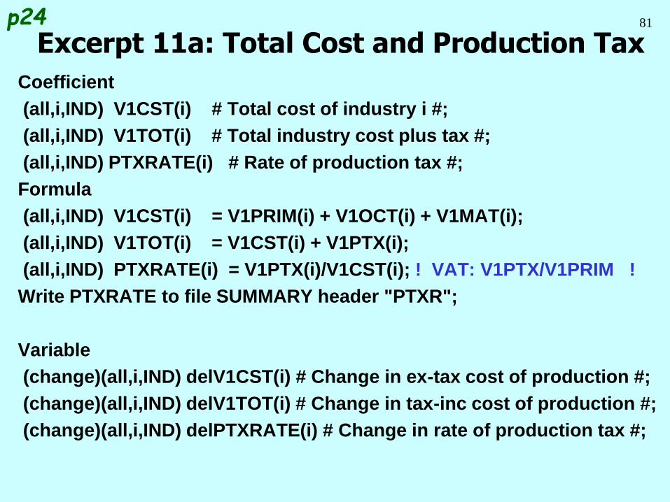
Coefficient
(all,i,IND) V1CST(i) # Total cost of industry i #;
(all,i,IND) V1TOT(i) # Total industry cost plus tax #;
(all,i,IND) PTXRATE(i) # Rate of production tax #;
Formula
(all,i,IND) V1CST(i) = V1PRIM(i) + V1OCT(i) + V1MAT(i);
(all,i,IND) V1TOT(i) = V1CST(i) + V1PTX(i);
(all,i,IND) PTXRATE(i) = V1PTX(i)/V1CST(i); ! VAT: V1PTX/V1PRIM !
Write PTXRATE to file SUMMARY header "PTXR";
Variable
(change)(all,i,IND) delV1CST(i) # Change in ex-tax cost of production #;
(change)(all,i,IND) delV1TOT(i) # Change in tax-inc cost of production #;
(change)(all,i,IND) delPTXRATE(i) # Change in rate of production tax #;
Excerpt 11a: Total Cost and Production Taxp24
82
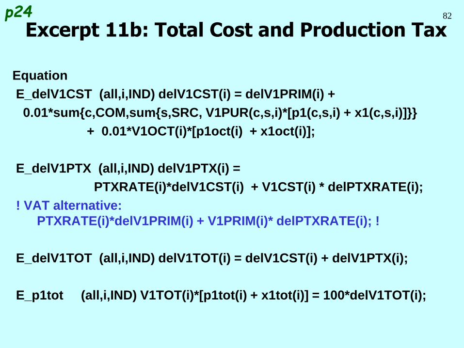
Equation
E_delV1CST (all,i,IND) delV1CST(i) = delV1PRIM(i) +
0.01*sum{c,COM,sum{s,SRC, V1PUR(c,s,i)*[p1(c,s,i) + x1(c,s,i)]}}
+ 0.01*V1OCT(i)*[p1oct(i) + x1oct(i)];
E_delV1PTX (all,i,IND) delV1PTX(i) =
PTXRATE(i)*delV1CST(i) + V1CST(i) * delPTXRATE(i);
! VAT alternative:
PTXRATE(i)*delV1PRIM(i) + V1PRIM(i)* delPTXRATE(i); !
E_delV1TOT (all,i,IND) delV1TOT(i) = delV1CST(i) + delV1PTX(i);
E_p1tot (all,i,IND) V1TOT(i)*[p1tot(i) + x1tot(i)] = 100*delV1TOT(i);
Excerpt 11b: Total Cost and Production Taxp24
83
Progress so far . . .
Introduction Inventory demands
Database structure Margin demands
Solution method Market clearing
TABLO language Price equations
Production: input decisions Aggregates and indices
Production: output decisions Investment allocation
Investment: input decisions Labour market
Household demands Decompositions
Export demands Closure
Government demands Regional extension
84
CET
up to Good GGood 2Good 1
Activity Level
CET
Local
Market
Export
Market
CET
Local
Market
Export
Market
V1TOT(i)
p1tot(i)
x1tot(i)
One Industry:
MAKE(c,i)
p0com(c)
q1(c,i)
DOMSALES(c)
p0dom(c)
x0dom(c)
All-Industry:
SALES(c)
p0com(c)
x0com(c)
V4BAS(c)
pe(c)
x4(c)
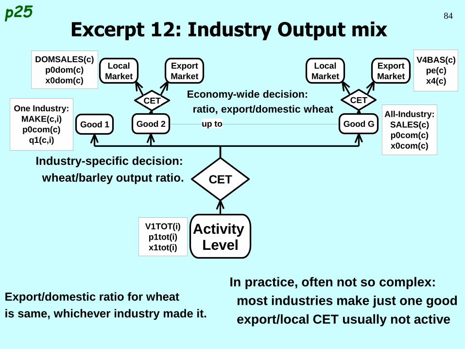
In practice, often not so complex:
most industries make just one good
export/local CET usually not active
Excerpt 12: Industry Output mixp25
Economy-wide decision:
ratio, export/domestic wheat
Industry-specific decision:
wheat/barley output ratio.
Export/domestic ratio for wheat
is same, whichever industry made it.
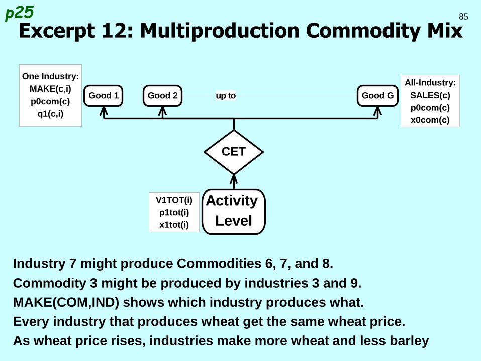
85
Industry 7 might produce Commodities 6, 7, and 8.
Commodity 3 might be produced by industries 3 and 9.
MAKE(COM,IND) shows which industry produces what.
Every industry that produces wheat get the same wheat price.
As wheat price rises, industries make more wheat and less barley
Excerpt 12: Multiproduction Commodity Mixp25
CET
up to Good GGood 2Good 1
Activity
Level
V1TOT(i)
p1tot(i)
x1tot(i)
One Industry:
MAKE(c,i)
p0com(c)
q1(c,i)
All-Industry:
SALES(c)
p0com(c)
x0com(c)
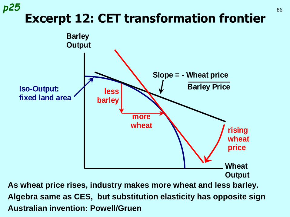
86
As wheat price rises, industry makes more wheat and less barley.
Algebra same as CES, but substitution elasticity has opposite sign
Australian invention: Powell/Gruen
Excerpt 12: CET transformation frontierp25
Barley Output
Wheat Output
Slope = - Wheat price
rising wheat price
Iso-Output: fixed land area
more wheat
less barley
Barley Price
87
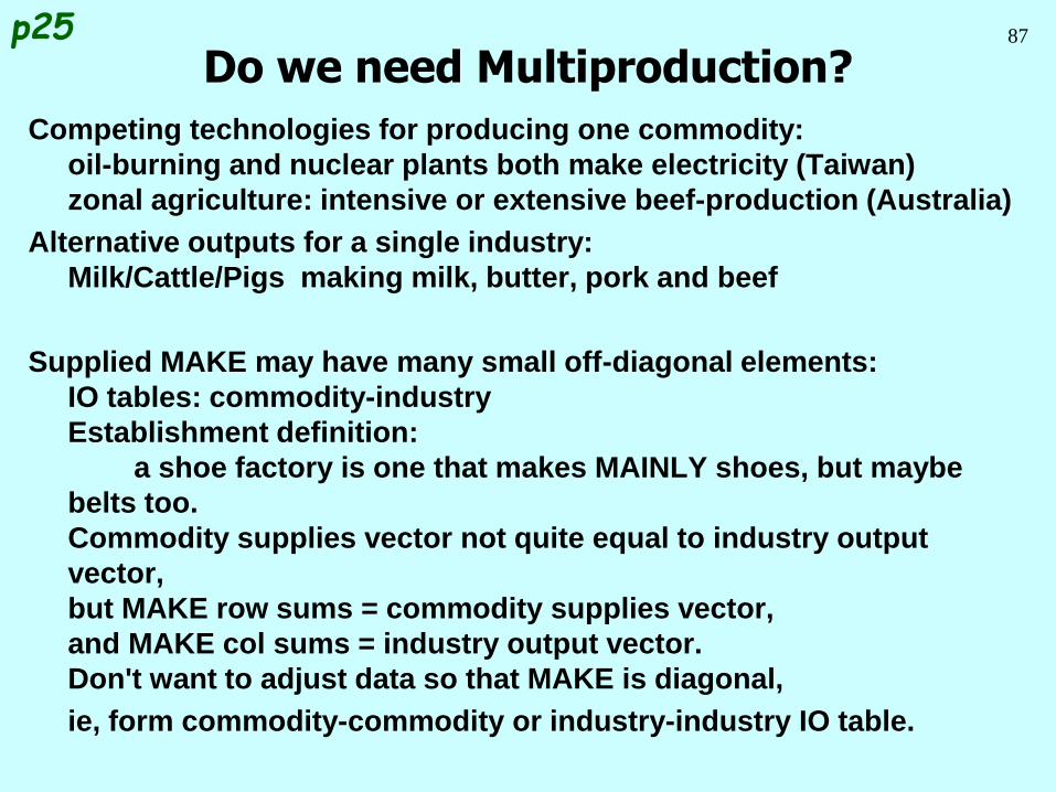
Competing technologies for producing one commodity:
oil-burning and nuclear plants both make electricity (Taiwan)
zonal agriculture: intensive or extensive beef-production (Australia)
Alternative outputs for a single industry:
Milk/Cattle/Pigs making milk, butter, pork and beef
Supplied MAKE may have many small off-diagonal elements:
IO tables: commodity-industry
Establishment definition:
a shoe factory is one that makes MAINLY shoes, but maybe
belts too.
Commodity supplies vector not quite equal to industry output
vector,
but MAKE row sums = commodity supplies vector,
and MAKE col sums = industry output vector.
Don't want to adjust data so that MAKE is diagonal,
ie, form commodity-commodity or industry-industry IO table.
Do we need Multiproduction?p25
88
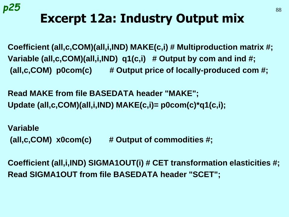
Coefficient (all,c,COM)(all,i,IND) MAKE(c,i) # Multiproduction matrix #;
Variable (all,c,COM)(all,i,IND) q1(c,i) # Output by com and ind #;
(all,c,COM) p0com(c) # Output price of locally-produced com #;
Read MAKE from file BASEDATA header "MAKE";
Update (all,c,COM)(all,i,IND) MAKE(c,i)= p0com(c)*q1(c,i);
Variable
(all,c,COM) x0com(c) # Output of commodities #;
Coefficient (all,i,IND) SIGMA1OUT(i) # CET transformation elasticities #;
Read SIGMA1OUT from file BASEDATA header "SCET";
Excerpt 12a: Industry Output mixp25
89
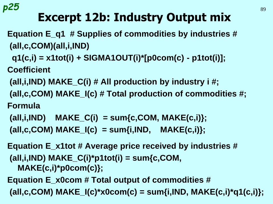
Equation E_q1 # Supplies of commodities by industries #
(all,c,COM)(all,i,IND)
q1(c,i) = x1tot(i) + SIGMA1OUT(i)*[p0com(c) - p1tot(i)];
Coefficient
(all,i,IND) MAKE_C(i) # All production by industry i #;
(all,c,COM) MAKE_I(c) # Total production of commodities #;
Formula
(all,i,IND) MAKE_C(i) = sum{c,COM, MAKE(c,i)};
(all,c,COM) MAKE_I(c) = sum{i,IND, MAKE(c,i)};
Equation E_x1tot # Average price received by industries #
(all,i,IND) MAKE_C(i)*p1tot(i) = sum{c,COM,
MAKE(c,i)*p0com(c)};
Equation E_x0com # Total output of commodities #
(all,c,COM) MAKE_I(c)*x0com(c) = sum{i,IND, MAKE(c,i)*q1(c,i)};
Excerpt 12b: Industry Output mixp25
90
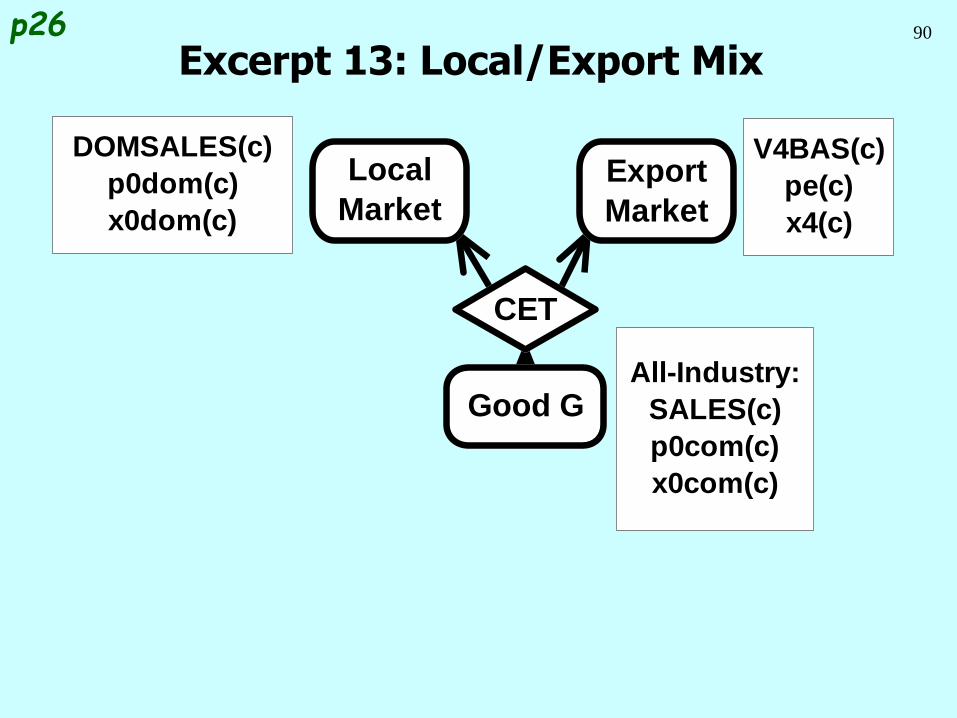
Excerpt 13: Local/Export Mixp26
Good G
CET
Local
Market
Export
Market
DOMSALES(c)
p0dom(c)
x0dom(c)
All-Industry:
SALES(c)
p0com(c)
x0com(c)
V4BAS(c)
pe(c)
x4(c)
91
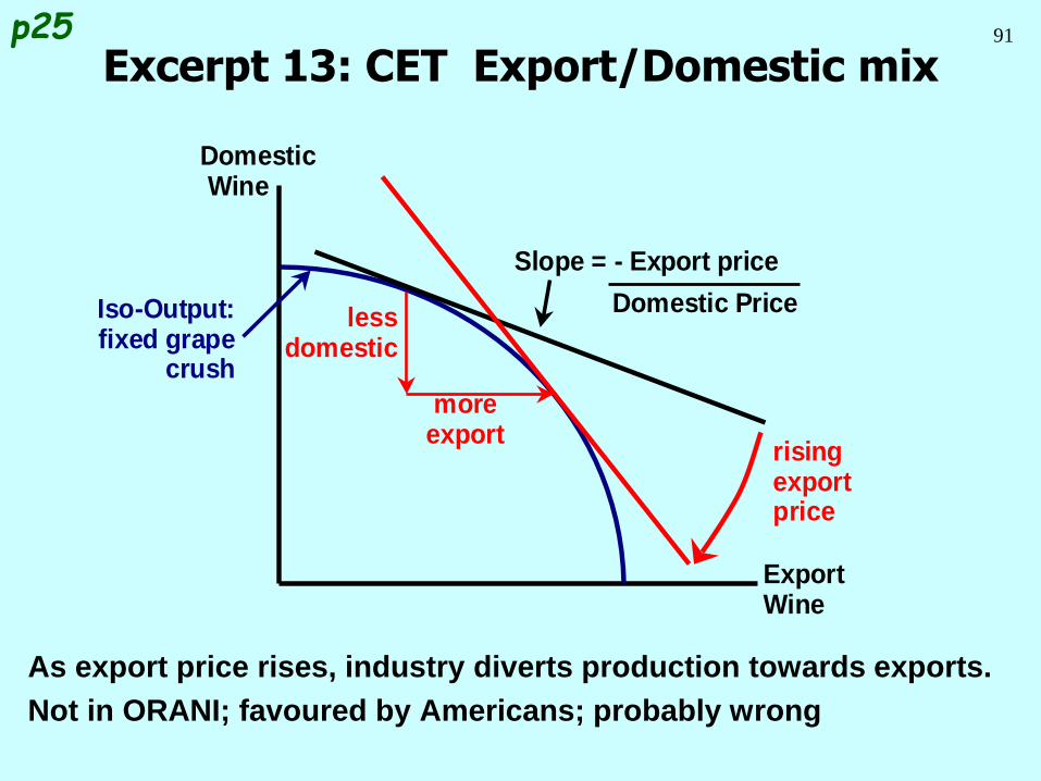
As export price rises, industry diverts production towards exports.
Not in ORANI; favoured by Americans; probably wrong
Excerpt 13: CET Export/Domestic mixp25
Domestic Wine
ExportWine
Slope = - Export price
rising export price
Iso-Output: fixed grape
crush more
export
less domestic
Domestic Price
92
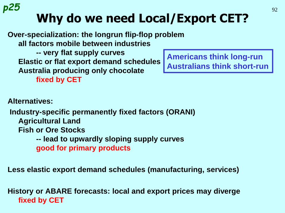
Over-specialization: the longrun flip-flop problem
all factors mobile between industries
-- very flat supply curves
Elastic or flat export demand schedules
Australia producing only chocolate
fixed by CET
Alternatives:
Industry-specific permanently fixed factors (ORANI)
Agricultural Land
Fish or Ore Stocks
-- lead to upwardly sloping supply curves
good for primary products
Less elastic export demand schedules (manufacturing, services)
History or ABARE forecasts: local and export prices may diverge
fixed by CET
Why do we need Local/Export CET?p25
Americans think long-run
Australians think short-run
93
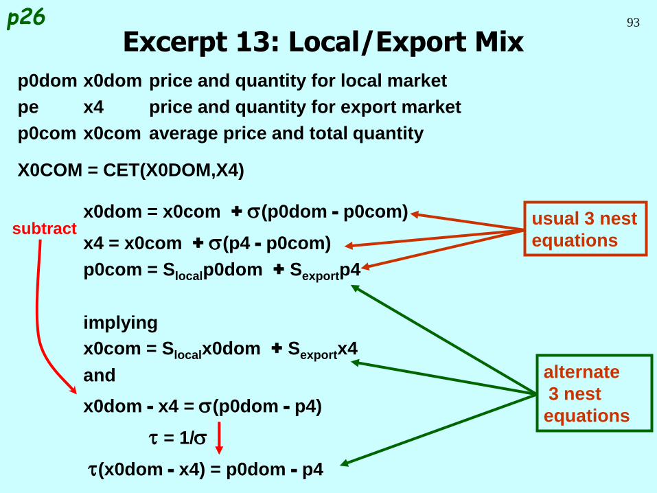
p0dom x0dom price and quantity for local market
pe x4 price and quantity for export market
p0com x0com average price and total quantity
X0COM = CET(X0DOM,X4)
x0dom = x0com + s(p0dom - p0com)
x4 = x0com + s(p4 - p0com)
p0com = Slocalp0dom + Sexportp4
implying
x0com = Slocalx0dom + Sexportx4
and
x0dom - x4 = s(p0dom - p4)
t = 1/s
t(x0dom - x4) = p0dom - p4
Excerpt 13: Local/Export Mixp26
usual 3 nest
equationssubtract
alternate
3 nest
equations
94
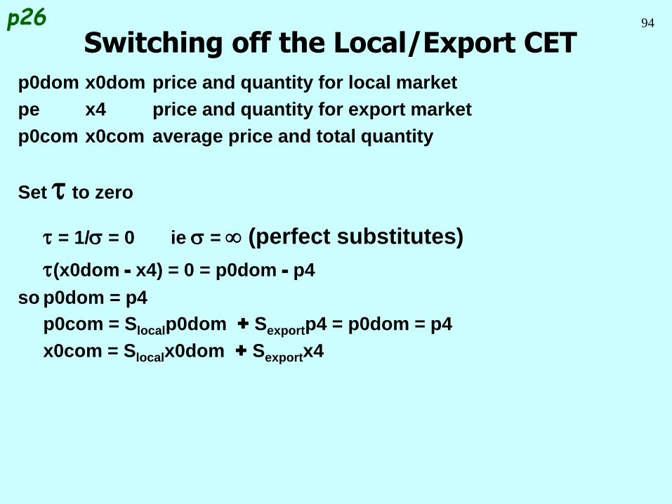
p0dom x0dom price and quantity for local market
pe x4 price and quantity for export market
p0com x0com average price and total quantity
Set t to zero
t = 1/s = 0 ie s = (perfect substitutes)
t(x0dom - x4) = 0 = p0dom - p4
so p0dom = p4
p0com = Slocalp0dom + Sexportp4 = p0dom = p4
x0com = Slocalx0dom + Sexportx4
Switching off the Local/Export CETp26
95
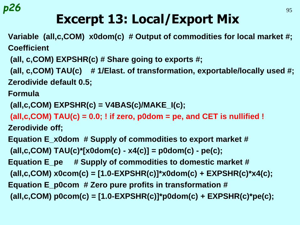
Variable (all,c,COM) x0dom(c) # Output of commodities for local market #;
Coefficient
(all, c,COM) EXPSHR(c) # Share going to exports #;
(all, c,COM) TAU(c) # 1/Elast. of transformation, exportable/locally used #;
Zerodivide default 0.5;
Formula
(all,c,COM) EXPSHR(c) = V4BAS(c)/MAKE_I(c);
(all,c,COM) TAU(c) = 0.0; ! if zero, p0dom = pe, and CET is nullified !
Zerodivide off;
Equation E_x0dom # Supply of commodities to export market #
(all,c,COM) TAU(c)*[x0dom(c) - x4(c)] = p0dom(c) - pe(c);
Equation E_pe # Supply of commodities to domestic market #
(all,c,COM) x0com(c) = [1.0-EXPSHR(c)]*x0dom(c) + EXPSHR(c)*x4(c);
Equation E_p0com # Zero pure profits in transformation #
(all,c,COM) p0com(c) = [1.0-EXPSHR(c)]*p0dom(c) + EXPSHR(c)*pe(c);
Excerpt 13: Local/Export Mixp26
96
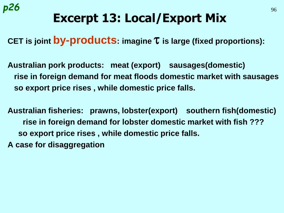
CET is joint by-products: imagine t is large (fixed proportions):
Australian pork products: meat (export) sausages(domestic)
rise in foreign demand for meat floods domestic market with sausages
so export price rises , while domestic price falls.
Australian fisheries: prawns, lobster(export) southern fish(domestic)
rise in foreign demand for lobster domestic market with fish ???
so export price rises , while domestic price falls.
A case for disaggregation
Excerpt 13: Local/Export Mixp26
97
Progress so far . . .
Introduction Inventory demands
Database structure Margin demands
Solution method Market clearing
TABLO language Price equations
Production: input decisions Aggregates and indices
Production: output decisions Investment allocation
Investment: input decisions Labour market
Household demands Decompositions
Export demands Closure
Government demands Regional extension
98
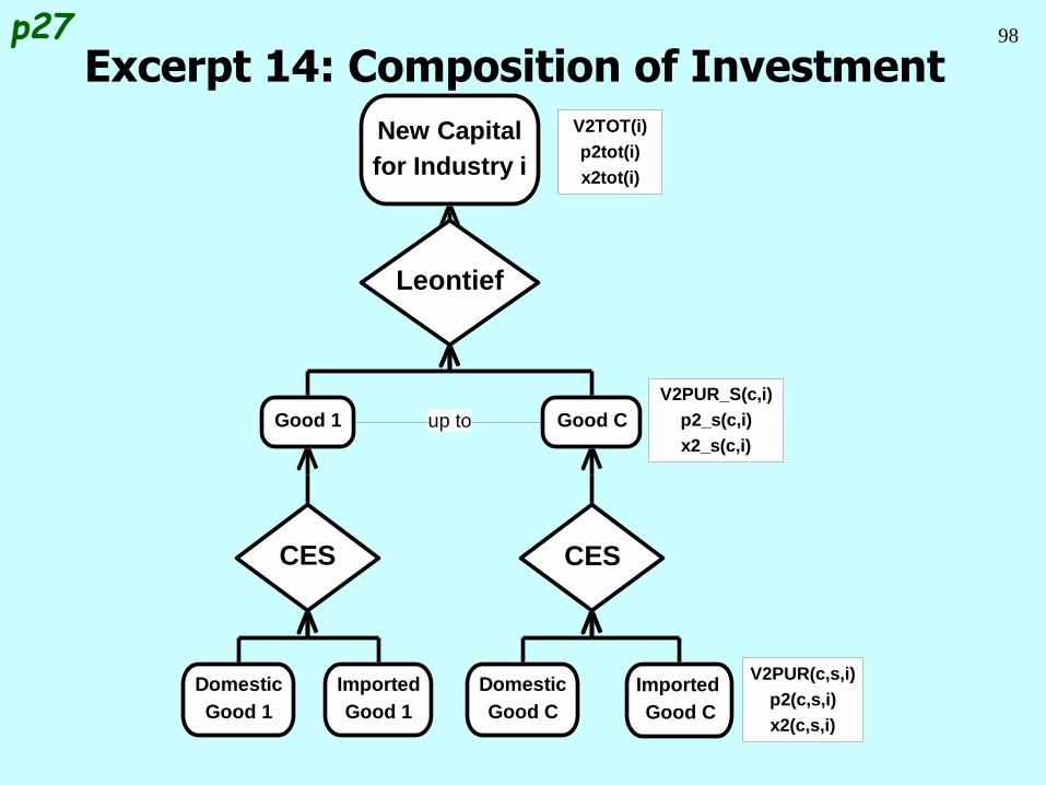
Excerpt 14: Composition of Investmentp27
Leontief
CESCES
up to
Imported
Good C
Domestic
Good C
Imported
Good 1
Domestic
Good 1
Good CGood 1
New Capital
for Industry i
V2TOT(i)
p2tot(i)
x2tot(i)
V2PUR_S(c,i)
p2_s(c,i)
x2_s(c,i)
V2PUR(c,s,i)
p2(c,s,i)
x2(c,s,i)
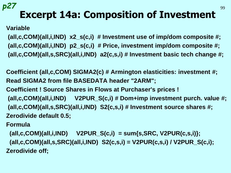
99
Variable
(all,c,COM)(all,i,IND) x2_s(c,i) # Investment use of imp/dom composite #;
(all,c,COM)(all,i,IND) p2_s(c,i) # Price, investment imp/dom composite #;
(all,c,COM)(all,s,SRC)(all,i,IND) a2(c,s,i) # Investment basic tech change #;
Coefficient (all,c,COM) SIGMA2(c) # Armington elasticities: investment #;
Read SIGMA2 from file BASEDATA header "2ARM";
Coefficient ! Source Shares in Flows at Purchaser's prices !
(all,c,COM)(all,i,IND) V2PUR_S(c,i) # Dom+imp investment purch. value #;
(all,c,COM)(all,s,SRC)(all,i,IND) S2(c,s,i) # Investment source shares #;
Zerodivide default 0.5;
Formula
(all,c,COM)(all,i,IND) V2PUR_S(c,i) = sum{s,SRC, V2PUR(c,s,i)};
(all,c,COM)(all,s,SRC)(all,i,IND) S2(c,s,i) = V2PUR(c,s,i) / V2PUR_S(c,i);
Zerodivide off;
Excerpt 14a: Composition of Investmentp27
100
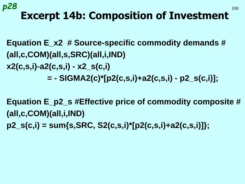
Equation E_x2 # Source-specific commodity demands #
(all,c,COM)(all,s,SRC)(all,i,IND)
x2(c,s,i)-a2(c,s,i) - x2_s(c,i)
= - SIGMA2(c)*[p2(c,s,i)+a2(c,s,i) - p2_s(c,i)];
Equation E_p2_s #Effective price of commodity composite #
(all,c,COM)(all,i,IND)
p2_s(c,i) = sum{s,SRC, S2(c,s,i)*[p2(c,s,i)+a2(c,s,i)]};
Excerpt 14b: Composition of Investmentp28
101
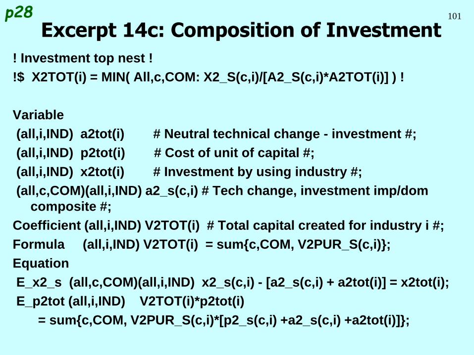
! Investment top nest !
!$ X2TOT(i) = MIN( All,c,COM: X2_S(c,i)/[A2_S(c,i)*A2TOT(i)] ) !
Variable
(all,i,IND) a2tot(i) # Neutral technical change - investment #;
(all,i,IND) p2tot(i) # Cost of unit of capital #;
(all,i,IND) x2tot(i) # Investment by using industry #;
(all,c,COM)(all,i,IND) a2_s(c,i) # Tech change, investment imp/dom
composite #;
Coefficient (all,i,IND) V2TOT(i) # Total capital created for industry i #;
Formula (all,i,IND) V2TOT(i) = sum{c,COM, V2PUR_S(c,i)};
Equation
E_x2_s (all,c,COM)(all,i,IND) x2_s(c,i) - [a2_s(c,i) + a2tot(i)] = x2tot(i);
E_p2tot (all,i,IND) V2TOT(i)*p2tot(i)
= sum{c,COM, V2PUR_S(c,i)*[p2_s(c,i) +a2_s(c,i) +a2tot(i)]};
Excerpt 14c: Composition of Investmentp28
102
Progress so far . . .
Introduction Inventory demands
Database structure Margin demands
Solution method Market clearing
TABLO language Price equations
Production: input decisions Aggregates and indices
Production: output decisions Investment allocation
Investment: input decisions Labour market
Household demands Decompositions
Export demands Closure
Government demands Regional extension
103
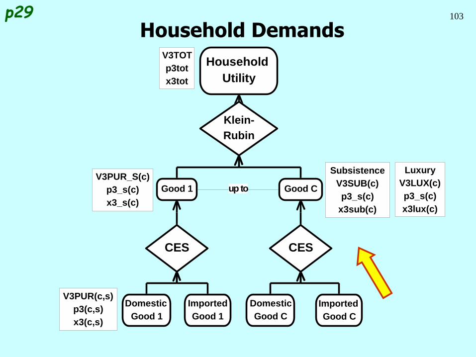
Klein-
Rubin
CESCES
up to
Imported
Good C
Domestic
Good C
Imported
Good 1
Domestic
Good 1
Good CGood 1
Household
Utility
V3TOT
p3tot
x3tot
V3PUR(c,s)
p3(c,s)
x3(c,s)
V3PUR_S(c)
p3_s(c)
x3_s(c)
Subsistence
V3SUB(c)
p3_s(c)
x3sub(c)
Luxury
V3LUX(c)
p3_s(c)
x3lux(c)
Household Demandsp29
104
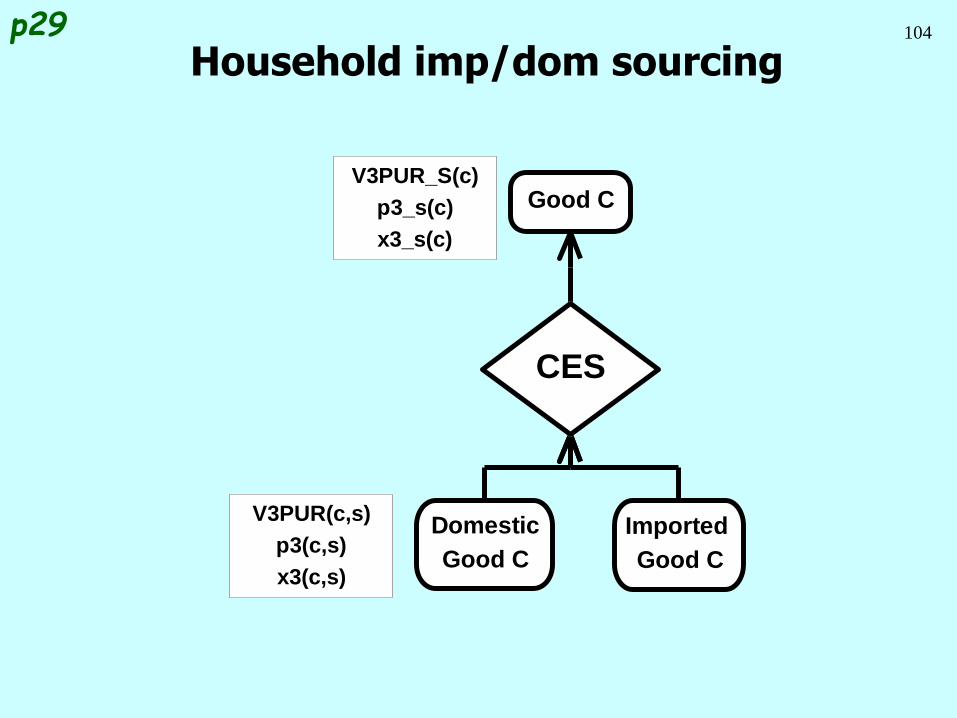
Household imp/dom sourcingp29
CES
Imported
Good C
Domestic
Good C
Good C
V3PUR(c,s)
p3(c,s)
x3(c,s)
V3PUR_S(c)
p3_s(c)
x3_s(c)
105
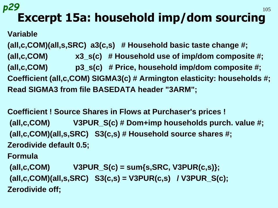
Variable
(all,c,COM)(all,s,SRC) a3(c,s) # Household basic taste change #;
(all,c,COM) x3_s(c) # Household use of imp/dom composite #;
(all,c,COM) p3_s(c) # Price, household imp/dom composite #;
Coefficient (all,c,COM) SIGMA3(c) # Armington elasticity: households #;
Read SIGMA3 from file BASEDATA header "3ARM";
Coefficient ! Source Shares in Flows at Purchaser's prices !
(all,c,COM) V3PUR_S(c) # Dom+imp households purch. value #;
(all,c,COM)(all,s,SRC) S3(c,s) # Household source shares #;
Zerodivide default 0.5;
Formula
(all,c,COM) V3PUR_S(c) = sum{s,SRC, V3PUR(c,s)};
(all,c,COM)(all,s,SRC) S3(c,s) = V3PUR(c,s) / V3PUR_S(c);
Zerodivide off;
Excerpt 15a: household imp/dom sourcingp29
106
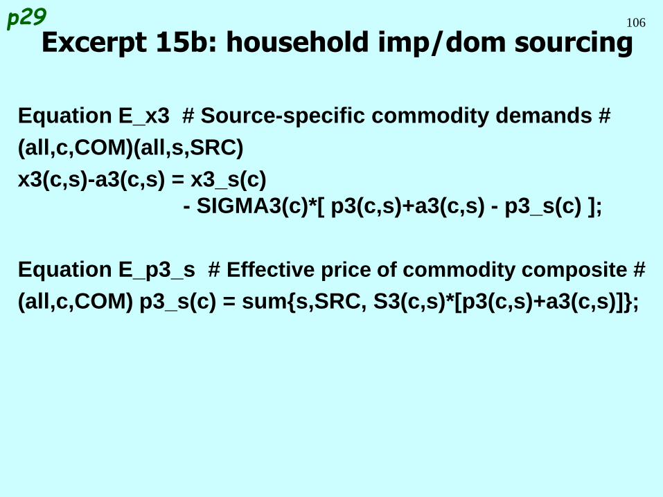
Equation E_x3 # Source-specific commodity demands #
(all,c,COM)(all,s,SRC)
x3(c,s)-a3(c,s) = x3_s(c)
- SIGMA3(c)*[ p3(c,s)+a3(c,s) - p3_s(c) ];
Equation E_p3_s # Effective price of commodity composite #
(all,c,COM) p3_s(c) = sum{s,SRC, S3(c,s)*[p3(c,s)+a3(c,s)]};
Excerpt 15b: household imp/dom sourcingp29
107Numerical Example of CES demands
•
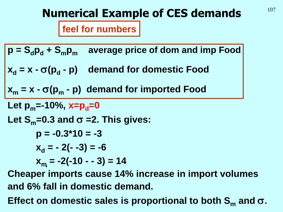
p = Sdpd + Smpm average price of dom and imp Food
xd = x - s(pd - p) demand for domestic Food
xm = x - s(pm - p) demand for imported Food
Let pm=-10%, x=pd=0
Let Sm=0.3 and s =2. This gives:
p = -0.3*10 = -3
xd = - 2(- -3) = -6
xm = -2(-10 - - 3) = 14
Cheaper imports cause 14% increase in import volumes
and 6% fall in domestic demand.
Effect on domestic sales is proportional to both Sm and s.
feel for numbers
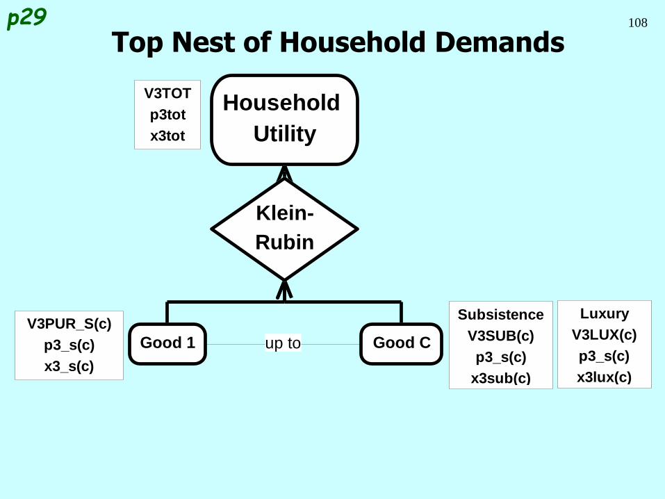
108
Top Nest of Household Demandsp29
Klein-
Rubin
up to Good CGood 1
Household
Utility
V3TOT
p3tot
x3tot
V3PUR_S(c)
p3_s(c)
x3_s(c)
Subsistence
V3SUB(c)
p3_s(c)
x3sub(c)
Luxury
V3LUX(c)
p3_s(c)
x3lux(c)
109Klein-Rubin:a non-homothetic utility function
p29
Homothetic means:
budget shares depend only on prices, not incomes
eg: CES, Cobb-Douglas
Non-homothetic means:
rising income causes budget shares to change
even with price ratios fixed.
Non-unitary expenditure elasticities:
1% rise in total expenditure might cause food expenditure
to rise by 1/2%; air travel expenditure to rise by 2%.
See Green Book for algebraic derivation (complex).
Explained here by a metaphor.
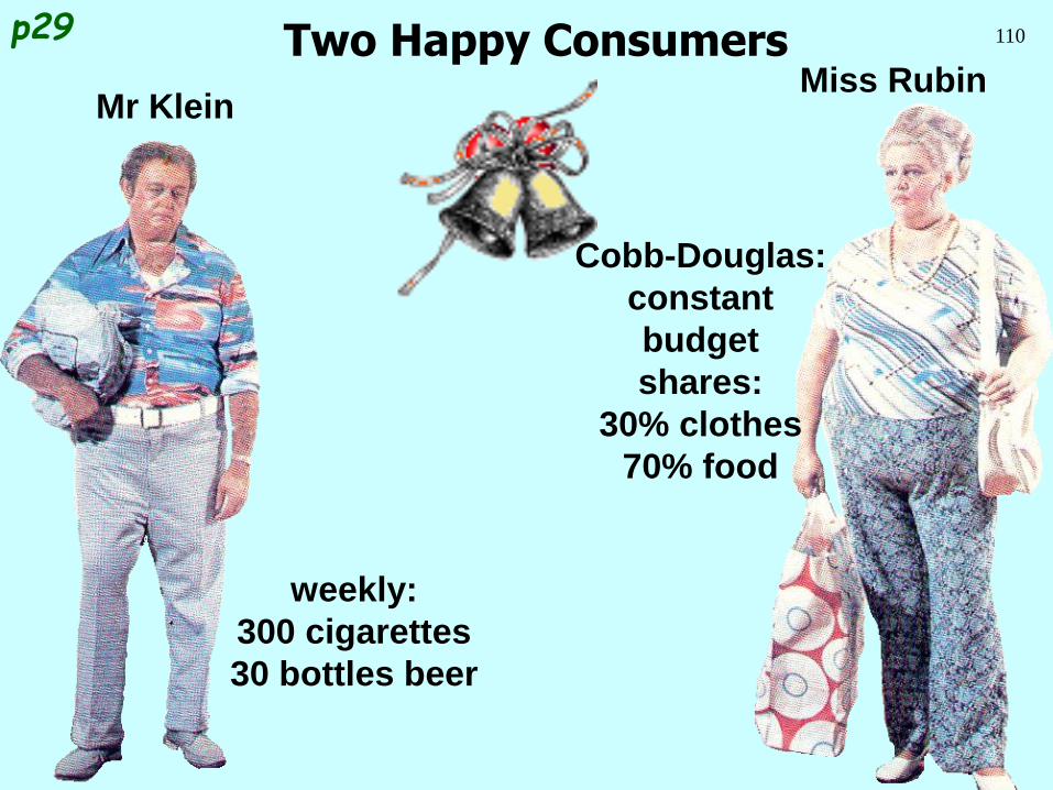
110Two Happy Consumersp29
weekly:
300 cigarettes
30 bottles beer
Mr Klein
Cobb-Douglas:
constant
budget
shares:
30% clothes
70% food
Miss Rubin
111
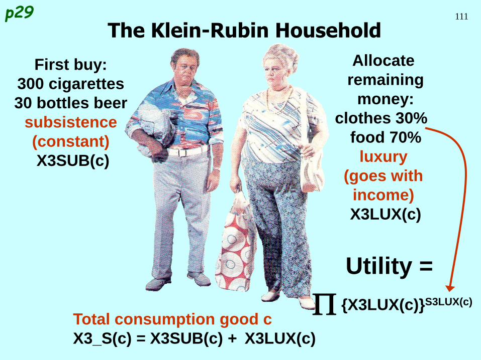
The Klein-Rubin Householdp29
Allocate
remaining
money:
clothes 30%
food 70%
luxury
(goes with
income)
X3LUX(c)
First buy:
300 cigarettes
30 bottles beer
subsistence
(constant)
X3SUB(c)
Utility =
P {X3LUX(c)}S3LUX(c)
Total consumption good c
X3_S(c) = X3SUB(c) + X3LUX(c)
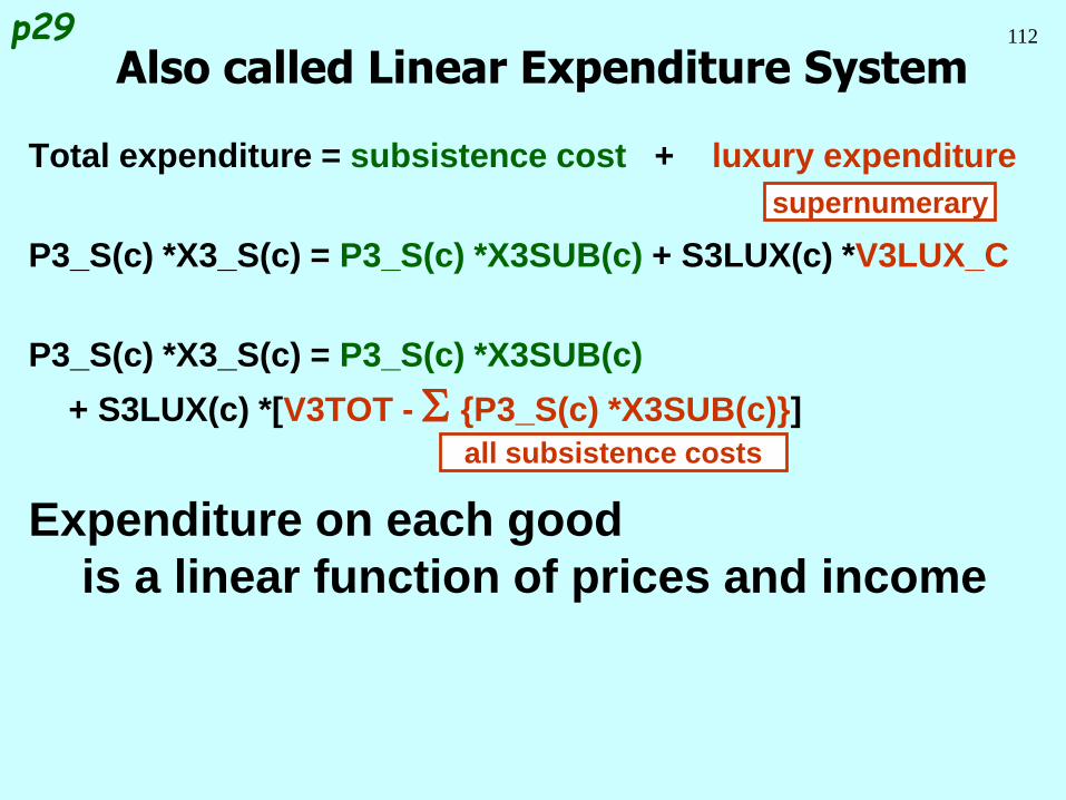
112
Total expenditure = subsistence cost + luxury expenditure
P3_S(c) *X3_S(c) = P3_S(c) *X3SUB(c) + S3LUX(c) *V3LUX_C
P3_S(c) *X3_S(c) = P3_S(c) *X3SUB(c)
+ S3LUX(c) *[V3TOT - S {P3_S(c) *X3SUB(c)}]
Expenditure on each good
is a linear function of prices and income
Also called Linear Expenditure Systemp29
supernumerary
all subsistence costs
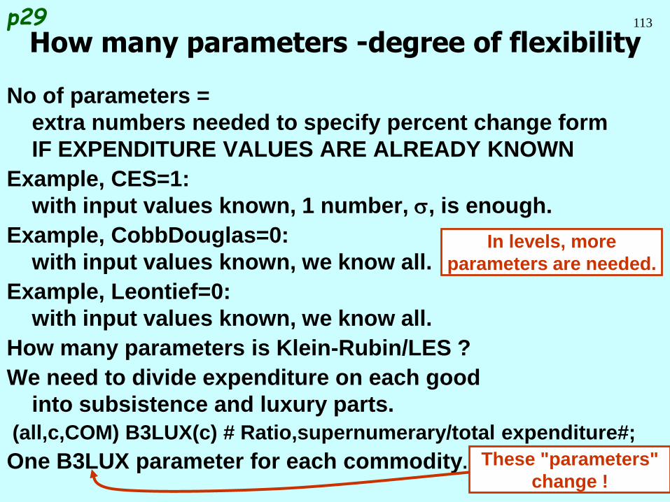
113
No of parameters =
extra numbers needed to specify percent change form
IF EXPENDITURE VALUES ARE ALREADY KNOWN
Example, CES=1:
with input values known, 1 number, s, is enough.
Example, CobbDouglas=0:
with input values known, we know all.
Example, Leontief=0:
with input values known, we know all.
How many parameters is Klein-Rubin/LES ?
We need to divide expenditure on each good
into subsistence and luxury parts.
(all,c,COM) B3LUX(c) # Ratio,supernumerary/total expenditure#;
One B3LUX parameter for each commodity.
How many parameters -degree of flexibilityp29
In levels, more
parameters are needed.
These "parameters"
change !
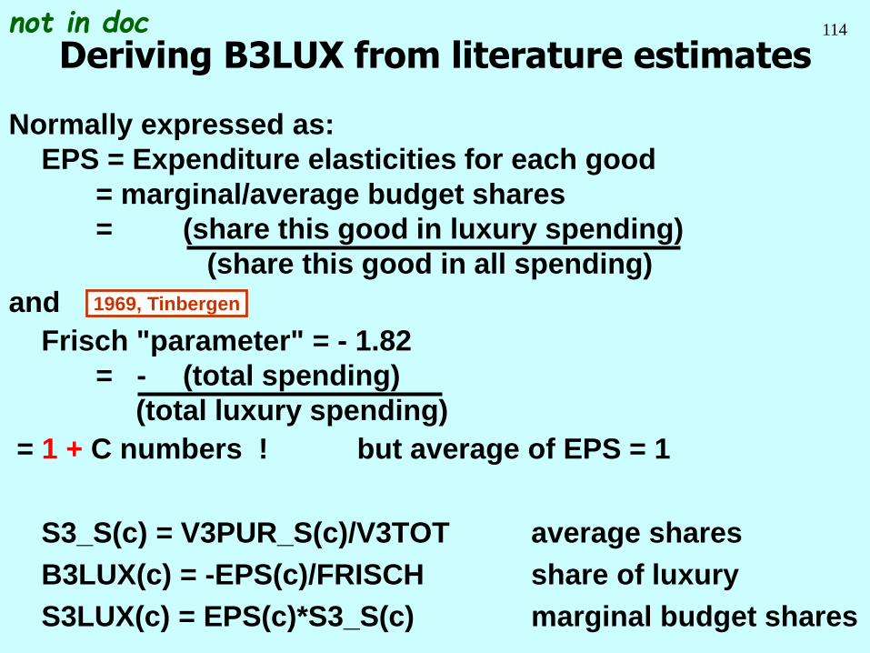
114
Normally expressed as:
EPS = Expenditure elasticities for each good
= marginal/average budget shares
= (share this good in luxury spending)
(share this good in all spending)
and
Frisch "parameter" = - 1.82
= - (total spending)
(total luxury spending)
= 1 + C numbers ! but average of EPS = 1
S3_S(c) = V3PUR_S(c)/V3TOT average shares
B3LUX(c) = -EPS(c)/FRISCH share of luxury
S3LUX(c) = EPS(c)*S3_S(c) marginal budget shares
Deriving B3LUX from literature estimatesnot in doc
1969, Tinbergen
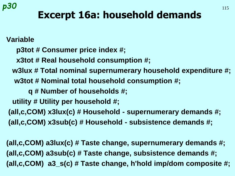
115
Variable
p3tot # Consumer price index #;
x3tot # Real household consumption #;
w3lux # Total nominal supernumerary household expenditure #;
w3tot # Nominal total household consumption #;
q # Number of households #;
utility # Utility per household #;
(all,c,COM) x3lux(c) # Household - supernumerary demands #;
(all,c,COM) x3sub(c) # Household - subsistence demands #;
(all,c,COM) a3lux(c) # Taste change, supernumerary demands #;
(all,c,COM) a3sub(c) # Taste change, subsistence demands #;
(all,c,COM) a3_s(c) # Taste change, h'hold imp/dom composite #;
Excerpt 16a: household demandsp30
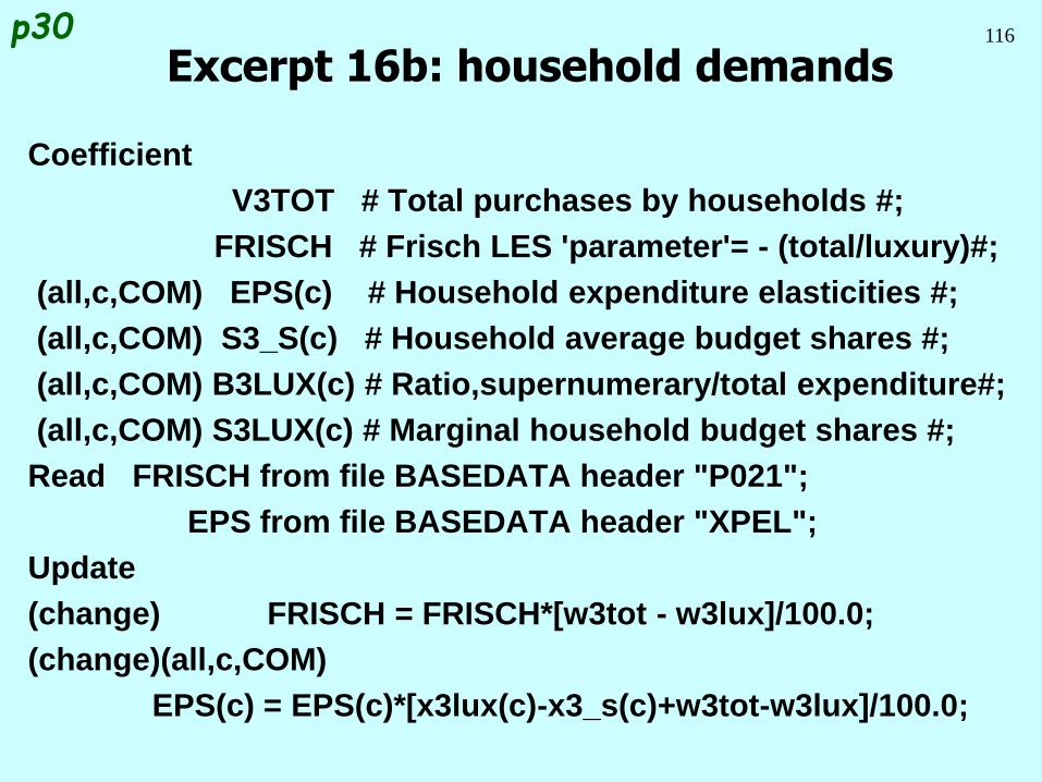
116
Coefficient
V3TOT # Total purchases by households #;
FRISCH # Frisch LES 'parameter'= - (total/luxury)#;
(all,c,COM) EPS(c) # Household expenditure elasticities #;
(all,c,COM) S3_S(c) # Household average budget shares #;
(all,c,COM) B3LUX(c) # Ratio,supernumerary/total expenditure#;
(all,c,COM) S3LUX(c) # Marginal household budget shares #;
Read FRISCH from file BASEDATA header "P021";
EPS from file BASEDATA header "XPEL";
Update
(change) FRISCH = FRISCH*[w3tot - w3lux]/100.0;
(change)(all,c,COM)
EPS(c) = EPS(c)*[x3lux(c)-x3_s(c)+w3tot-w3lux]/100.0;
Excerpt 16b: household demandsp30
117
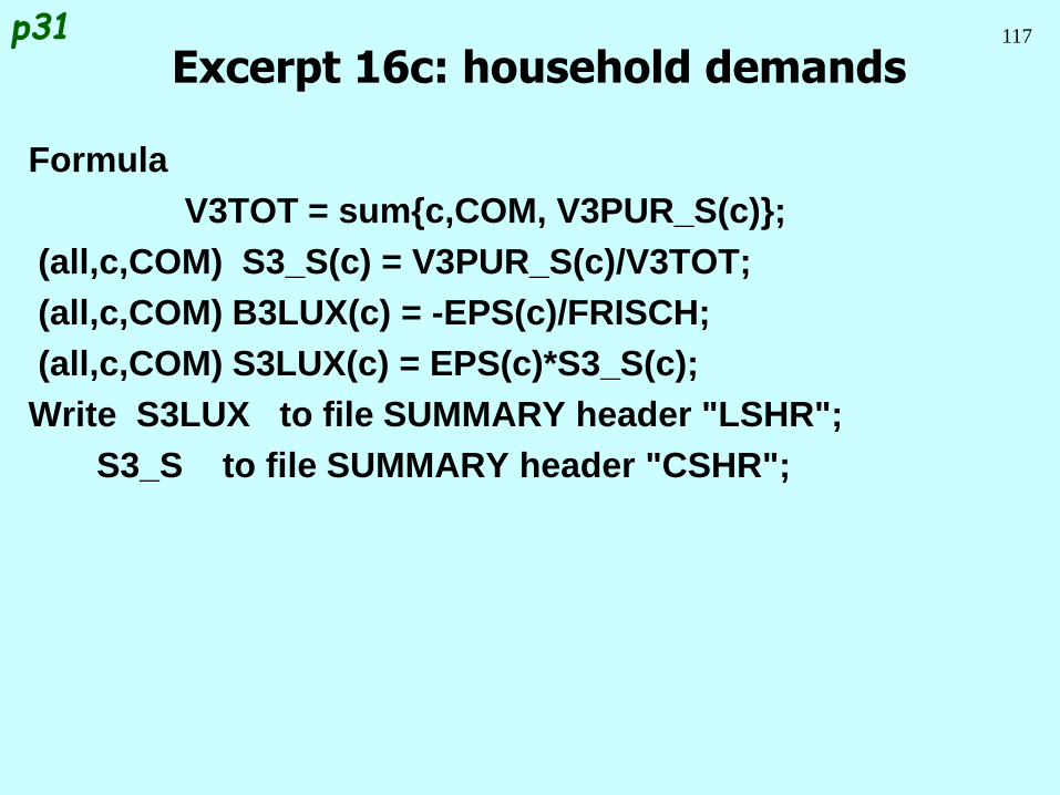
Formula
V3TOT = sum{c,COM, V3PUR_S(c)};
(all,c,COM) S3_S(c) = V3PUR_S(c)/V3TOT;
(all,c,COM) B3LUX(c) = -EPS(c)/FRISCH;
(all,c,COM) S3LUX(c) = EPS(c)*S3_S(c);
Write S3LUX to file SUMMARY header "LSHR";
S3_S to file SUMMARY header "CSHR";
Excerpt 16c: household demandsp31
118
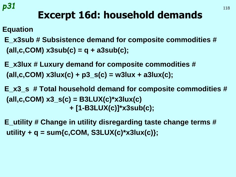
Equation
E_x3sub # Subsistence demand for composite commodities #
(all,c,COM) x3sub(c) = q + a3sub(c);
E_x3lux # Luxury demand for composite commodities #
(all,c,COM) x3lux(c) + p3_s(c) = w3lux + a3lux(c);
E_x3_s # Total household demand for composite commodities #
(all,c,COM) x3_s(c) = B3LUX(c)*x3lux(c)
+ [1-B3LUX(c)]*x3sub(c);
E_utility # Change in utility disregarding taste change terms #
utility + q = sum{c,COM, S3LUX(c)*x3lux(c)};
Excerpt 16d: household demandsp31
119
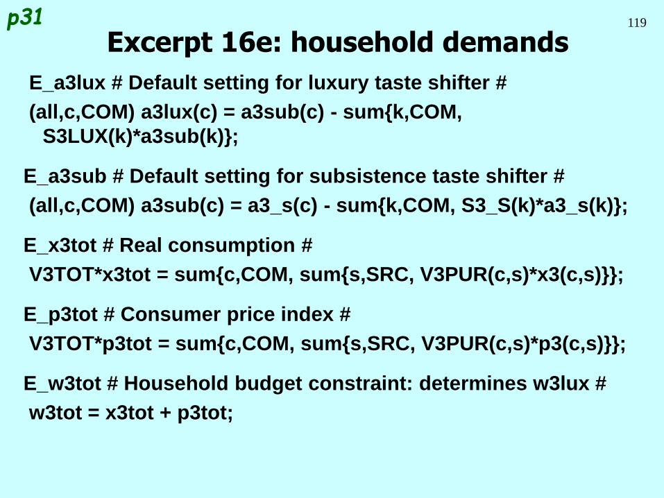
E_a3lux # Default setting for luxury taste shifter #
(all,c,COM) a3lux(c) = a3sub(c) - sum{k,COM,
S3LUX(k)*a3sub(k)};
E_a3sub # Default setting for subsistence taste shifter #
(all,c,COM) a3sub(c) = a3_s(c) - sum{k,COM, S3_S(k)*a3_s(k)};
E_x3tot # Real consumption #
V3TOT*x3tot = sum{c,COM, sum{s,SRC, V3PUR(c,s)*x3(c,s)}};
E_p3tot # Consumer price index #
V3TOT*p3tot = sum{c,COM, sum{s,SRC, V3PUR(c,s)*p3(c,s)}};
E_w3tot # Household budget constraint: determines w3lux #
w3tot = x3tot + p3tot;
Excerpt 16e: household demandsp31

120
Fact: with s = 1, CES is same as Cobb-Douglas.
Question: With all expenditure elasticities = 1,
is Klein-Rubin same as Cobb-Douglas ?
Quiz Questionp31
Answer: No. Would be Cobb-Douglas if Frisch
parameter = -1 [totally luxury]. Own-price
demand elasticity for Cobb-Douglas = -1;
average own-price demand elasticity for Klein-
Rubin is share of luxury in total spending
(maybe 0.5). Tendency towards inelastic
demand.
Stone-Geary = another name for Klein-Rubin
121
Progress so far . . .
Introduction Inventory demands
Database structure Margin demands
Solution method Market clearing
TABLO language Price equations
Production: input decisions Aggregates and indices
Production: output decisions Investment allocation
Investment: input decisions Labour market
Household demands Decompositions
Export demands Closure
Government demands Regional extension
122
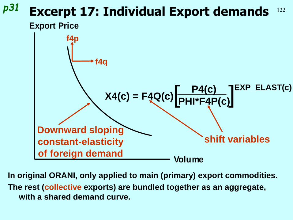
In original ORANI, only applied to main (primary) export commodities.
The rest (collective exports) are bundled together as an aggregate,
with a shared demand curve.
Excerpt 17: Individual Export demandsp31
Export Price
Volume
Downward sloping
constant-elasticity
of foreign demand
X4(c) = F4Q(c)[ P4(c)
PHI*F4P(c)]EXP_ELAST(c)
shift variables
f4q
f4p
123
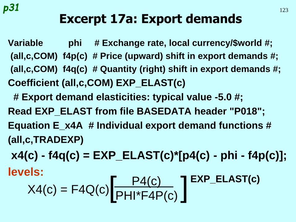
Variable phi # Exchange rate, local currency/$world #;
(all,c,COM) f4p(c) # Price (upward) shift in export demands #;
(all,c,COM) f4q(c) # Quantity (right) shift in export demands #;
Coefficient (all,c,COM) EXP_ELAST(c)
# Export demand elasticities: typical value -5.0 #;
Read EXP_ELAST from file BASEDATA header "P018";
Equation E_x4A # Individual export demand functions #
(all,c,TRADEXP)
x4(c) - f4q(c) = EXP_ELAST(c)*[p4(c) - phi - f4p(c)];
levels:
Excerpt 17a: Export demandsp31
X4(c) = F4Q(c)[ P4(c)
PHI*F4P(c) ]EXP_ELAST(c)
124
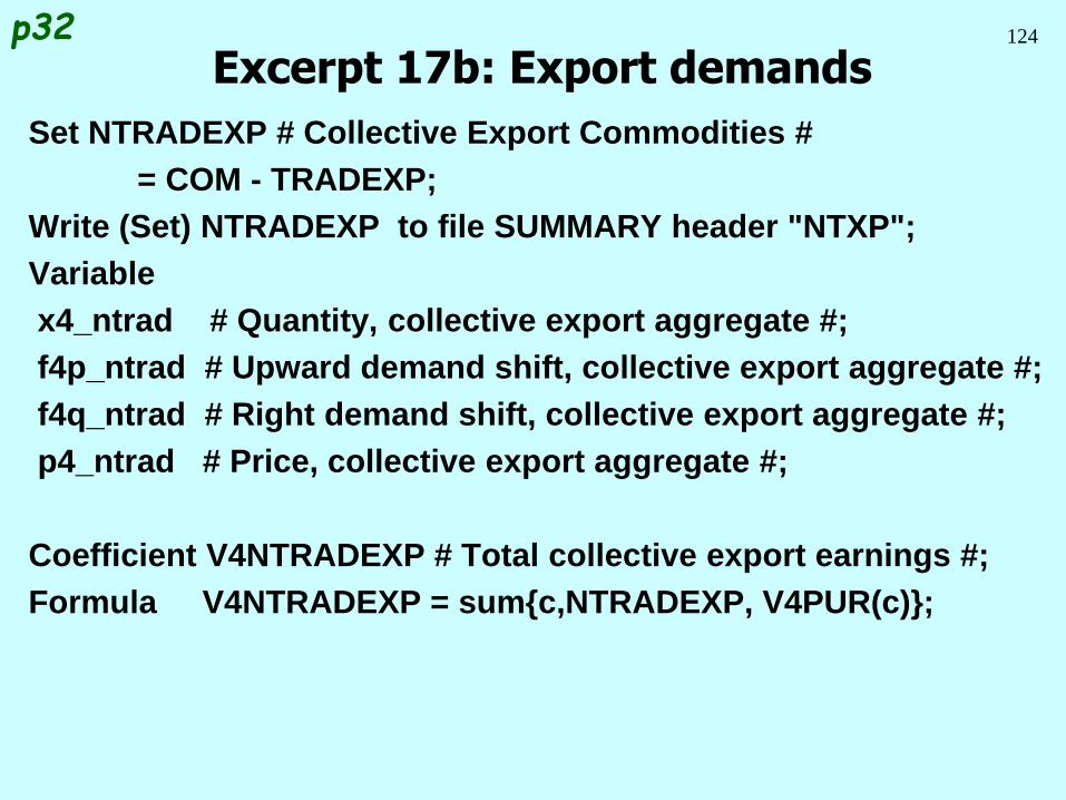
Set NTRADEXP # Collective Export Commodities #
= COM - TRADEXP;
Write (Set) NTRADEXP to file SUMMARY header "NTXP";
Variable
x4_ntrad # Quantity, collective export aggregate #;
f4p_ntrad # Upward demand shift, collective export aggregate #;
f4q_ntrad # Right demand shift, collective export aggregate #;
p4_ntrad # Price, collective export aggregate #;
Coefficient V4NTRADEXP # Total collective export earnings #;
Formula V4NTRADEXP = sum{c,NTRADEXP, V4PUR(c)};
Excerpt 17b: Export demandsp32
125
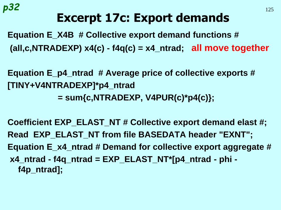
Equation E_X4B # Collective export demand functions #
(all,c,NTRADEXP) x4(c) - f4q(c) = x4_ntrad; all move together
Equation E_p4_ntrad # Average price of collective exports #
[TINY+V4NTRADEXP]*p4_ntrad
= sum{c,NTRADEXP, V4PUR(c)*p4(c)};
Coefficient EXP_ELAST_NT # Collective export demand elast #;
Read EXP_ELAST_NT from file BASEDATA header "EXNT";
Equation E_x4_ntrad # Demand for collective export aggregate #
x4_ntrad - f4q_ntrad = EXP_ELAST_NT*[p4_ntrad - phi -
f4p_ntrad];
Excerpt 17c: Export demandsp32
126
Progress so far . . .
Introduction Inventory demands
Database structure Margin demands
Solution method Market clearing
TABLO language Price equations
Production: input decisions Aggregates and indices
Production: output decisions Investment allocation
Investment: input decisions Labour market
Household demands Decompositions
Export demands Closure
Government demands Regional extension
127
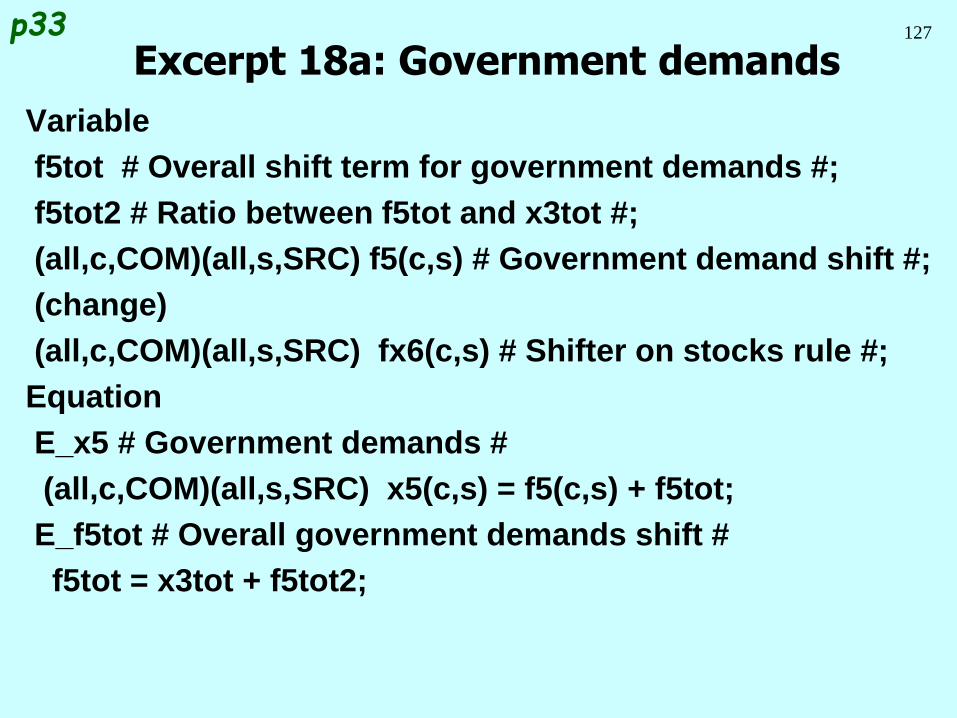
Variable
f5tot # Overall shift term for government demands #;
f5tot2 # Ratio between f5tot and x3tot #;
(all,c,COM)(all,s,SRC) f5(c,s) # Government demand shift #;
(change)
(all,c,COM)(all,s,SRC) fx6(c,s) # Shifter on stocks rule #;
Equation
E_x5 # Government demands #
(all,c,COM)(all,s,SRC) x5(c,s) = f5(c,s) + f5tot;
E_f5tot # Overall government demands shift #
f5tot = x3tot + f5tot2;
Excerpt 18a: Government demandsp33
128
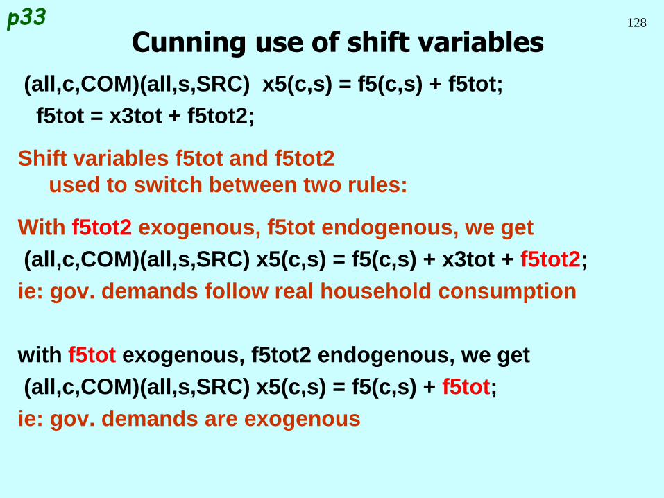
(all,c,COM)(all,s,SRC) x5(c,s) = f5(c,s) + f5tot;
f5tot = x3tot + f5tot2;
Shift variables f5tot and f5tot2
used to switch between two rules:
With f5tot2 exogenous, f5tot endogenous, we get
(all,c,COM)(all,s,SRC) x5(c,s) = f5(c,s) + x3tot + f5tot2;
ie: gov. demands follow real household consumption
with f5tot exogenous, f5tot2 endogenous, we get
(all,c,COM)(all,s,SRC) x5(c,s) = f5(c,s) + f5tot;
ie: gov. demands are exogenous
Cunning use of shift variablesp33
129
Progress so far . . .
Introduction Inventory demands
Database structure Margin demands
Solution method Market clearing
TABLO language Price equations
Production: input decisions Aggregates and indices
Production: output decisions Investment allocation
Investment: input decisions Labour market
Household demands Decompositions
Export demands Closure
Government demands Regional extension
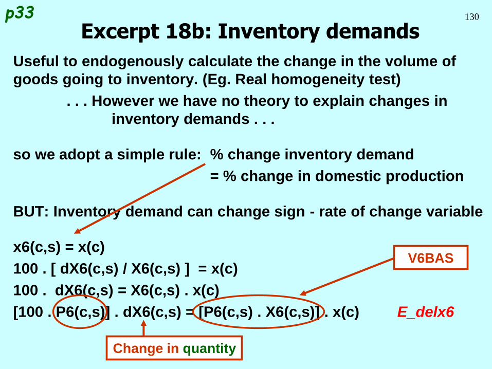
130
Useful to endogenously calculate the change in the volume of
goods going to inventory. (Eg. Real homogeneity test)
. . . However we have no theory to explain changes in
inventory demands . . .
so we adopt a simple rule: % change inventory demand
= % change in domestic production
BUT: Inventory demand can change sign - rate of change variable
x6(c,s) = x(c)
100 . [ dX6(c,s) / X6(c,s) ] = x(c)
100 . dX6(c,s) = X6(c,s) . x(c)
[100 . P6(c,s)] . dX6(c,s) = [P6(c,s) . X6(c,s)] . x(c) E_delx6
Excerpt 18b: Inventory demandsp33
V6BAS
Change in quantity
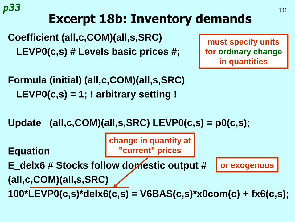
131
Coefficient (all,c,COM)(all,s,SRC)
LEVP0(c,s) # Levels basic prices #;
Formula (initial) (all,c,COM)(all,s,SRC)
LEVP0(c,s) = 1; ! arbitrary setting !
Update (all,c,COM)(all,s,SRC) LEVP0(c,s) = p0(c,s);
Equation
E_delx6 # Stocks follow domestic output #
(all,c,COM)(all,s,SRC)
100*LEVP0(c,s)*delx6(c,s) = V6BAS(c,s)*x0com(c) + fx6(c,s);
Excerpt 18b: Inventory demandsp33
must specify units
for ordinary change
in quantities
change in quantity at
"current" prices
or exogenous
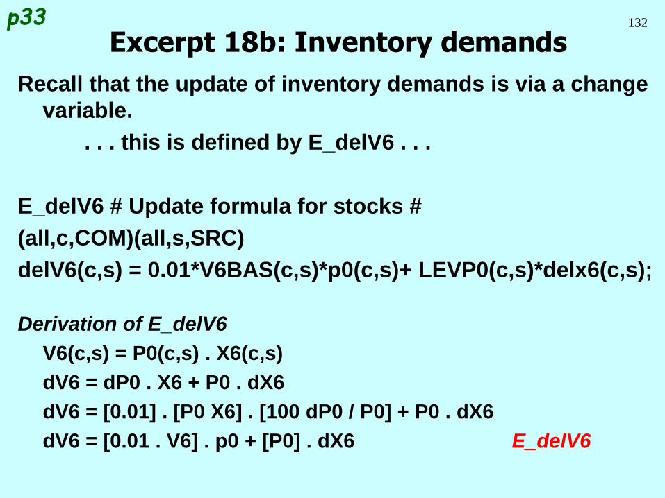
132
Recall that the update of inventory demands is via a change
variable.
. . . this is defined by E_delV6 . . .
E_delV6 # Update formula for stocks #
(all,c,COM)(all,s,SRC)
delV6(c,s) = 0.01*V6BAS(c,s)*p0(c,s)+ LEVP0(c,s)*delx6(c,s);
Derivation of E_delV6
V6(c,s) = P0(c,s) . X6(c,s)
dV6 = dP0 . X6 + P0 . dX6
dV6 = [0.01] . [P0 X6] . [100 dP0 / P0] + P0 . dX6
dV6 = [0.01 . V6] . p0 + [P0] . dX6 E_delV6
Excerpt 18b: Inventory demandsp33
133
Progress so far . . .
Introduction Inventory demands
Database structure Margin demands
Solution method Market clearing
TABLO language Price equations
Production: input decisions Aggregates and indices
Production: output decisions Investment allocation
Investment: input decisions Labour market
Household demands Decompositions
Export demands Closure
Government demands Regional extension
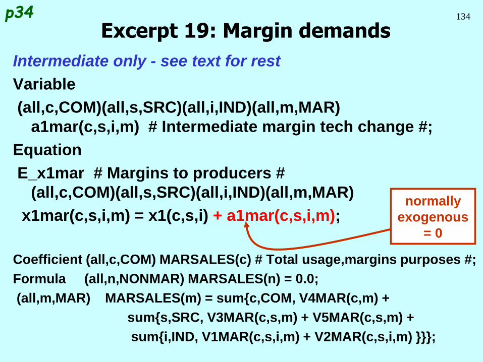
134
Intermediate only - see text for rest
Variable
(all,c,COM)(all,s,SRC)(all,i,IND)(all,m,MAR)
a1mar(c,s,i,m) # Intermediate margin tech change #;
Equation
E_x1mar # Margins to producers #
(all,c,COM)(all,s,SRC)(all,i,IND)(all,m,MAR)
x1mar(c,s,i,m) = x1(c,s,i) + a1mar(c,s,i,m);
Coefficient (all,c,COM) MARSALES(c) # Total usage,margins purposes #;
Formula (all,n,NONMAR) MARSALES(n) = 0.0;
(all,m,MAR) MARSALES(m) = sum{c,COM, V4MAR(c,m) +
sum{s,SRC, V3MAR(c,s,m) + V5MAR(c,s,m) +
sum{i,IND, V1MAR(c,s,i,m) + V2MAR(c,s,i,m) }}};
Excerpt 19: Margin demandsp34
normally
exogenous
= 0

135
Progress so far . . .
Introduction Inventory demands
Database structure Margin demands
Solution method Market clearing
TABLO language Price equations
Production: input decisions Aggregates and indices
Production: output decisions Investment allocation
Investment: input decisions Labour market
Household demands Decompositions
Export demands Closure
Government demands Regional extension
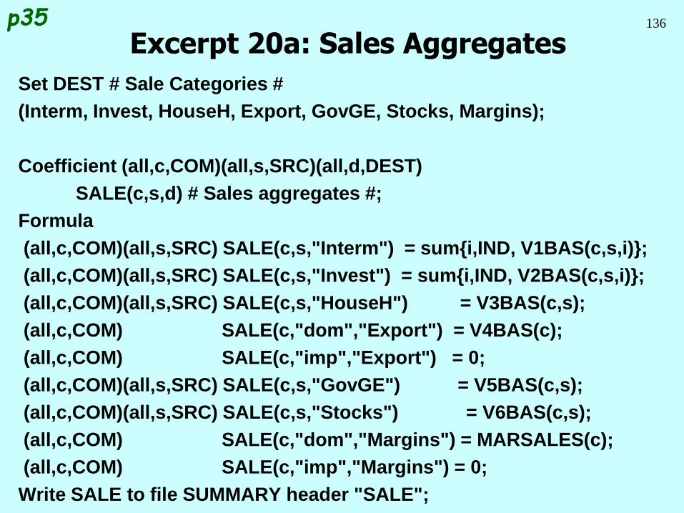
136
Set DEST # Sale Categories #
(Interm, Invest, HouseH, Export, GovGE, Stocks, Margins);
Coefficient (all,c,COM)(all,s,SRC)(all,d,DEST)
SALE(c,s,d) # Sales aggregates #;
Formula
(all,c,COM)(all,s,SRC) SALE(c,s,"Interm") = sum{i,IND, V1BAS(c,s,i)};
(all,c,COM)(all,s,SRC) SALE(c,s,"Invest") = sum{i,IND, V2BAS(c,s,i)};
(all,c,COM)(all,s,SRC) SALE(c,s,"HouseH") = V3BAS(c,s);
(all,c,COM) SALE(c,"dom","Export") = V4BAS(c);
(all,c,COM) SALE(c,"imp","Export") = 0;
(all,c,COM)(all,s,SRC) SALE(c,s,"GovGE") = V5BAS(c,s);
(all,c,COM)(all,s,SRC) SALE(c,s,"Stocks") = V6BAS(c,s);
(all,c,COM) SALE(c,"dom","Margins") = MARSALES(c);
(all,c,COM) SALE(c,"imp","Margins") = 0;
Write SALE to file SUMMARY header "SALE";
Excerpt 20a: Sales Aggregatesp35
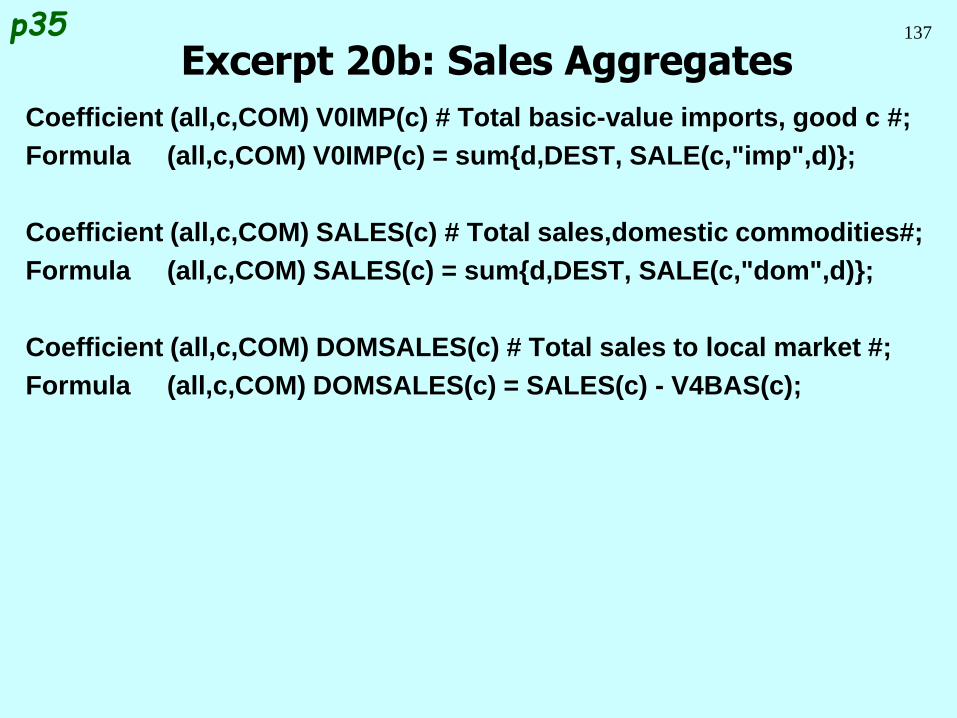
137
Coefficient (all,c,COM) V0IMP(c) # Total basic-value imports, good c #;
Formula (all,c,COM) V0IMP(c) = sum{d,DEST, SALE(c,"imp",d)};
Coefficient (all,c,COM) SALES(c) # Total sales,domestic commodities#;
Formula (all,c,COM) SALES(c) = sum{d,DEST, SALE(c,"dom",d)};
Coefficient (all,c,COM) DOMSALES(c) # Total sales to local market #;
Formula (all,c,COM) DOMSALES(c) = SALES(c) - V4BAS(c);
Excerpt 20b: Sales Aggregatesp35
138
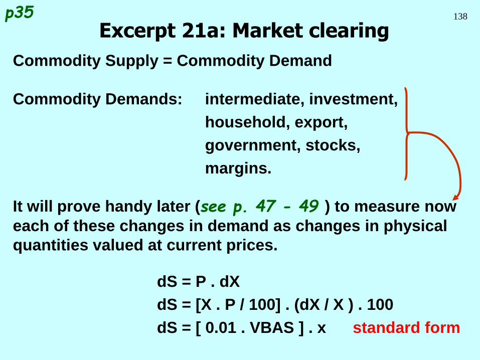
Commodity Supply = Commodity Demand
Commodity Demands: intermediate, investment,
household, export,
government, stocks,
margins.
It will prove handy later (see p. 47 - 49 ) to measure now
each of these changes in demand as changes in physical
quantities valued at current prices.
dS = P . dX
dS = [X . P / 100] . (dX / X ) . 100
dS = [ 0.01 . VBAS ] . x standard form
Excerpt 21a: Market clearingp35
139
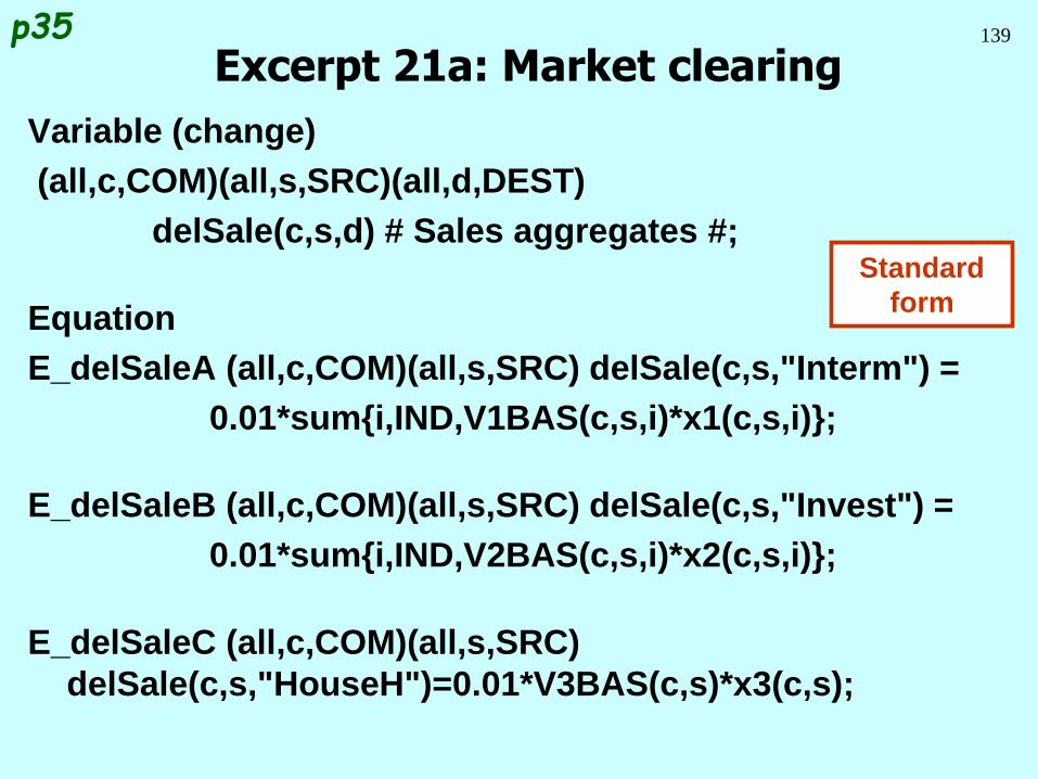
Variable (change)
(all,c,COM)(all,s,SRC)(all,d,DEST)
delSale(c,s,d) # Sales aggregates #;
Equation
E_delSaleA (all,c,COM)(all,s,SRC) delSale(c,s,"Interm") =
0.01*sum{i,IND,V1BAS(c,s,i)*x1(c,s,i)};
E_delSaleB (all,c,COM)(all,s,SRC) delSale(c,s,"Invest") =
0.01*sum{i,IND,V2BAS(c,s,i)*x2(c,s,i)};
E_delSaleC (all,c,COM)(all,s,SRC)
delSale(c,s,"HouseH")=0.01*V3BAS(c,s)*x3(c,s);
Excerpt 21a: Market clearingp35
Standard
form
140
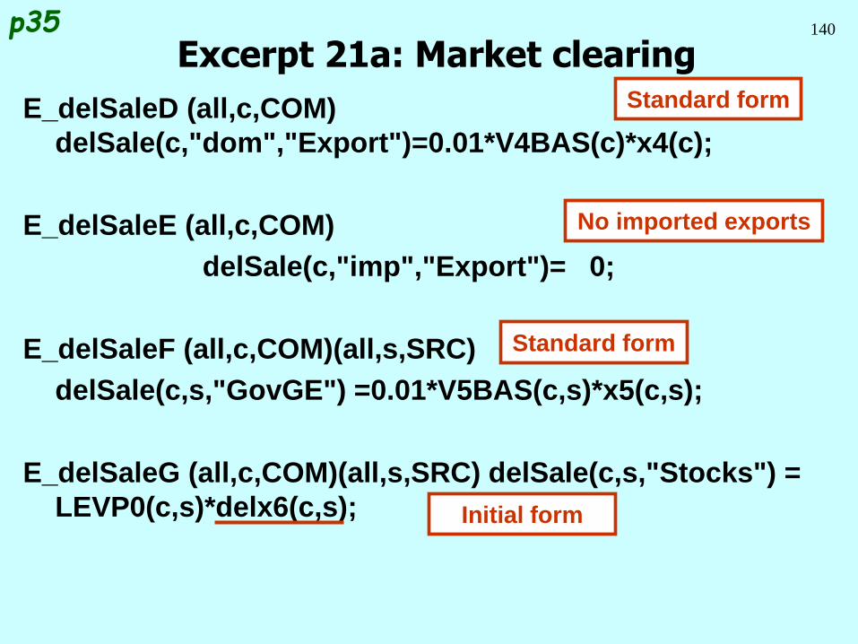
E_delSaleD (all,c,COM)
delSale(c,"dom","Export")=0.01*V4BAS(c)*x4(c);
E_delSaleE (all,c,COM)
delSale(c,"imp","Export")= 0;
E_delSaleF (all,c,COM)(all,s,SRC)
delSale(c,s,"GovGE") =0.01*V5BAS(c,s)*x5(c,s);
E_delSaleG (all,c,COM)(all,s,SRC) delSale(c,s,"Stocks") =
LEVP0(c,s)*delx6(c,s);
Excerpt 21a: Market clearingp35
Standard form
No imported exports
Standard form
Initial form
141
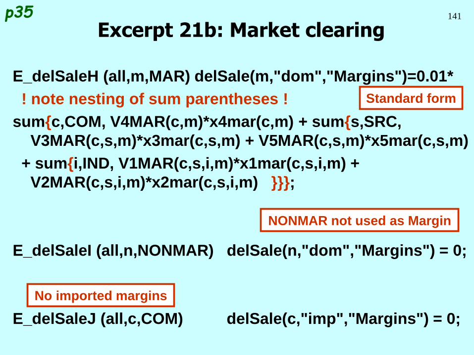
E_delSaleH (all,m,MAR) delSale(m,"dom","Margins")=0.01*
! note nesting of sum parentheses !
sum{c,COM, V4MAR(c,m)*x4mar(c,m) + sum{s,SRC,
V3MAR(c,s,m)*x3mar(c,s,m) + V5MAR(c,s,m)*x5mar(c,s,m)
+ sum{i,IND, V1MAR(c,s,i,m)*x1mar(c,s,i,m) +
V2MAR(c,s,i,m)*x2mar(c,s,i,m) }}};
E_delSaleI (all,n,NONMAR) delSale(n,"dom","Margins") = 0;
E_delSaleJ (all,c,COM) delSale(c,"imp","Margins") = 0;
Excerpt 21b: Market clearingp35
Standard form
NONMAR not used as Margin
No imported margins
142
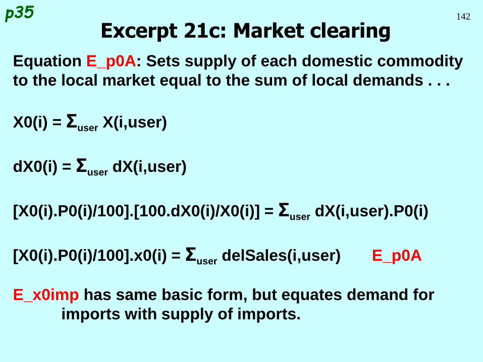
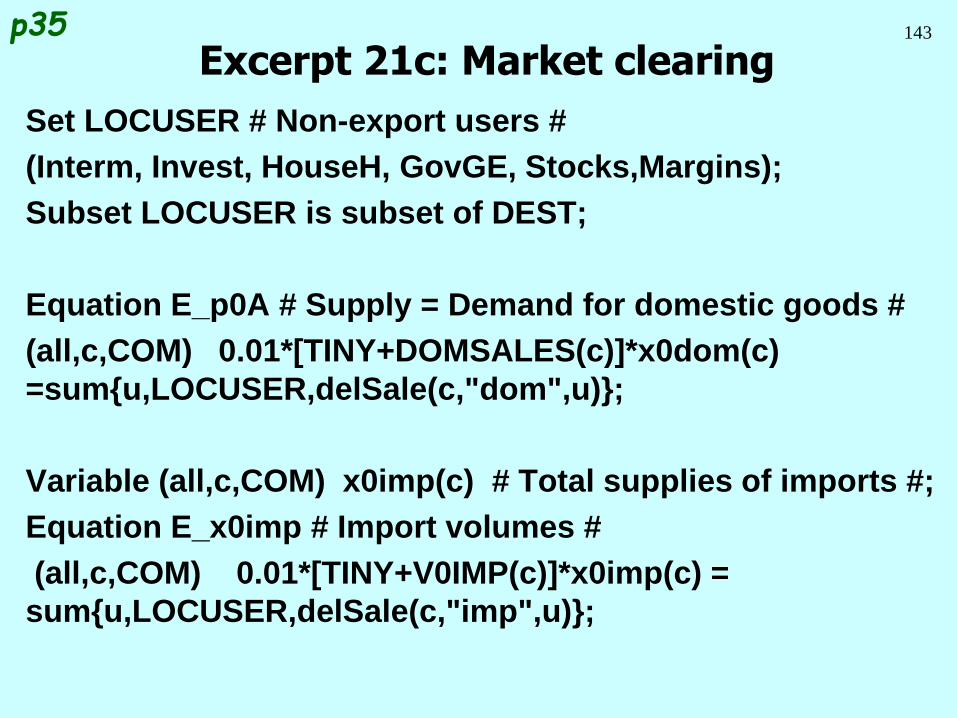
Equation E_p0A: Sets supply of each domestic commodity
to the local market equal to the sum of local demands . . .
X0(i) = Σuser X(i,user)
dX0(i) = Σuser dX(i,user)
[X0(i).P0(i)/100].[100.dX0(i)/X0(i)] = Σuser dX(i,user).P0(i)
[X0(i).P0(i)/100].x0(i) = Σuser delSales(i,user) E_p0A
E_x0imp has same basic form, but equates demand for
imports with supply of imports.
Excerpt 21c: Market clearingp35
143
Set LOCUSER # Non-export users #
(Interm, Invest, HouseH, GovGE, Stocks,Margins);
Subset LOCUSER is subset of DEST;
Equation E_p0A # Supply = Demand for domestic goods #
(all,c,COM) 0.01*[TINY+DOMSALES(c)]*x0dom(c)
=sum{u,LOCUSER,delSale(c,"dom",u)};
Variable (all,c,COM) x0imp(c) # Total supplies of imports #;
Equation E_x0imp # Import volumes #
(all,c,COM) 0.01*[TINY+V0IMP(c)]*x0imp(c) =
sum{u,LOCUSER,delSale(c,"imp",u)};
Excerpt 21c: Market clearingp35
144
Progress so far . . .
Introduction Inventory demands
Database structure Margin demands
Solution method Market clearing
TABLO language Price equations
Production: input decisions Aggregates and indices
Production: output decisions Investment allocation
Investment: input decisions Labour market
Household demands Decompositions
Export demands Closure
Government demands Regional extension
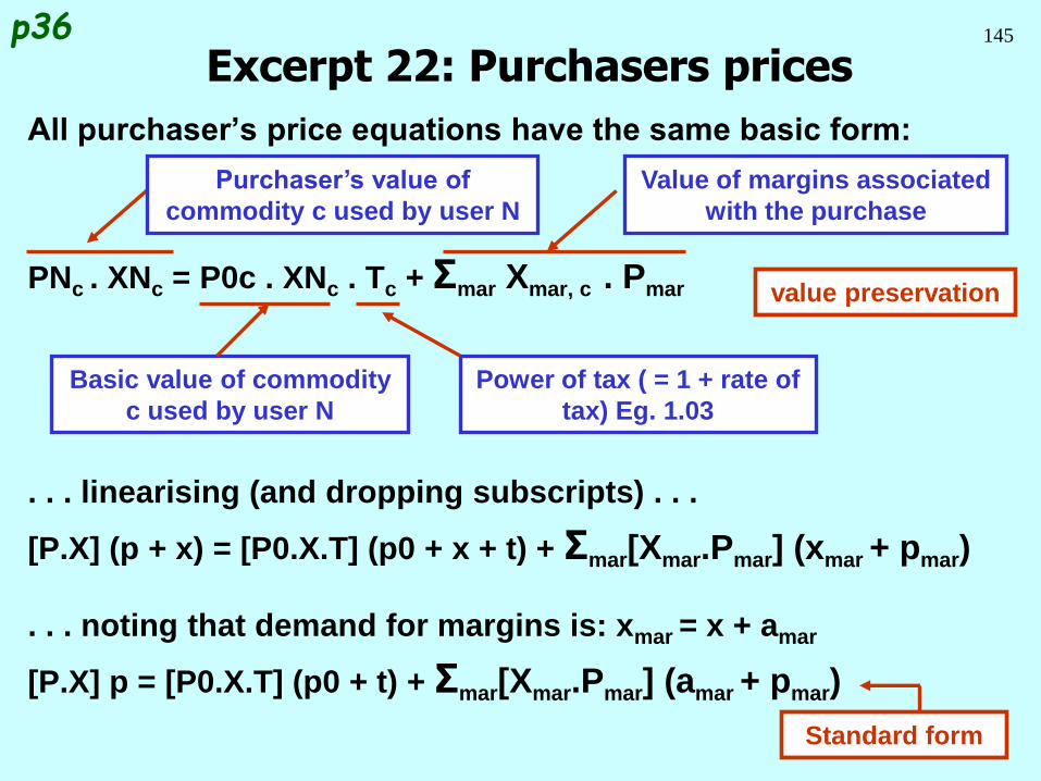
145
All purchaser’s price equations have the same basic form:
PNc . XNc = P0c . XNc . Tc + Σmar Xmar, c . Pmar
. . . linearising (and dropping subscripts) . . .
[P.X] (p + x) = [P0.X.T] (p0 + x + t) + Σmar[Xmar.Pmar] (xmar + pmar)
. . . noting that demand for margins is: xmar = x + amar
[P.X] p = [P0.X.T] (p0 + t) + Σmar[Xmar.Pmar] (amar + pmar)
Excerpt 22: Purchasers pricesp36
Purchaser’s value of
commodity c used by user N
Basic value of commodity
c used by user N
Power of tax ( = 1 + rate of
tax) Eg. 1.03
Value of margins associated
with the purchase
value preservation
Standard form
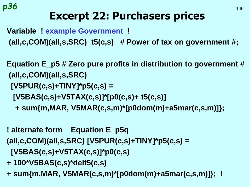
146
Variable ! example Government !
(all,c,COM)(all,s,SRC) t5(c,s) # Power of tax on government #;
Equation E_p5 # Zero pure profits in distribution to government #
(all,c,COM)(all,s,SRC)
[V5PUR(c,s)+TINY]*p5(c,s) =
[V5BAS(c,s)+V5TAX(c,s)]*[p0(c,s)+ t5(c,s)]
+ sum{m,MAR, V5MAR(c,s,m)*[p0dom(m)+a5mar(c,s,m)]};
! alternate form Equation E_p5q
(all,c,COM)(all,s,SRC) [V5PUR(c,s)+TINY]*p5(c,s) =
[V5BAS(c,s)+V5TAX(c,s)]*p0(c,s)
+ 100*V5BAS(c,s)*delt5(c,s)
+ sum{m,MAR, V5MAR(c,s,m)*[p0dom(m)+a5mar(c,s,m)]}; !
Excerpt 22: Purchasers pricesp36
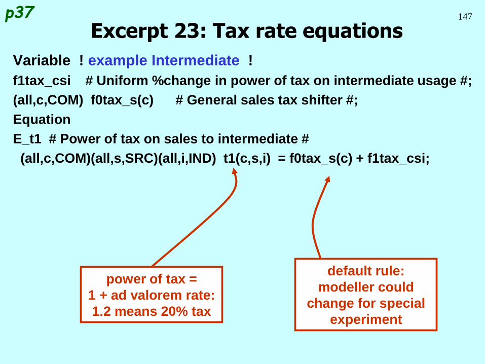
147
Variable ! example Intermediate !
f1tax_csi # Uniform %change in power of tax on intermediate usage #;
(all,c,COM) f0tax_s(c) # General sales tax shifter #;
Equation
E_t1 # Power of tax on sales to intermediate #
(all,c,COM)(all,s,SRC)(all,i,IND) t1(c,s,i) = f0tax_s(c) + f1tax_csi;
Excerpt 23: Tax rate equationsp37
default rule:
modeller could
change for special
experiment
power of tax =
1 + ad valorem rate:
1.2 means 20% tax
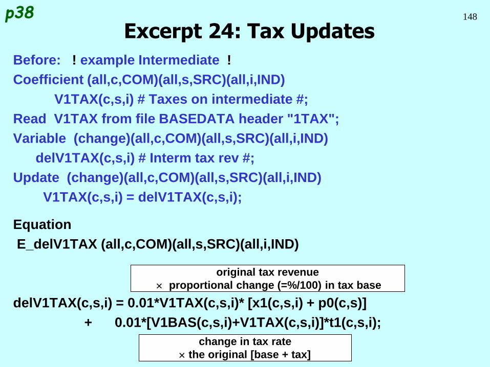
148
Before: ! example Intermediate !
Coefficient (all,c,COM)(all,s,SRC)(all,i,IND)
V1TAX(c,s,i) # Taxes on intermediate #;
Read V1TAX from file BASEDATA header "1TAX";
Variable (change)(all,c,COM)(all,s,SRC)(all,i,IND)
delV1TAX(c,s,i) # Interm tax rev #;
Update (change)(all,c,COM)(all,s,SRC)(all,i,IND)
V1TAX(c,s,i) = delV1TAX(c,s,i);
Equation
E_delV1TAX (all,c,COM)(all,s,SRC)(all,i,IND)
delV1TAX(c,s,i) = 0.01*V1TAX(c,s,i)* [x1(c,s,i) + p0(c,s)]
+ 0.01*[V1BAS(c,s,i)+V1TAX(c,s,i)]*t1(c,s,i);
Excerpt 24: Tax Updatesp38
change in tax rate
the original [base + tax]
original tax revenue
proportional change (=%/100) in tax base
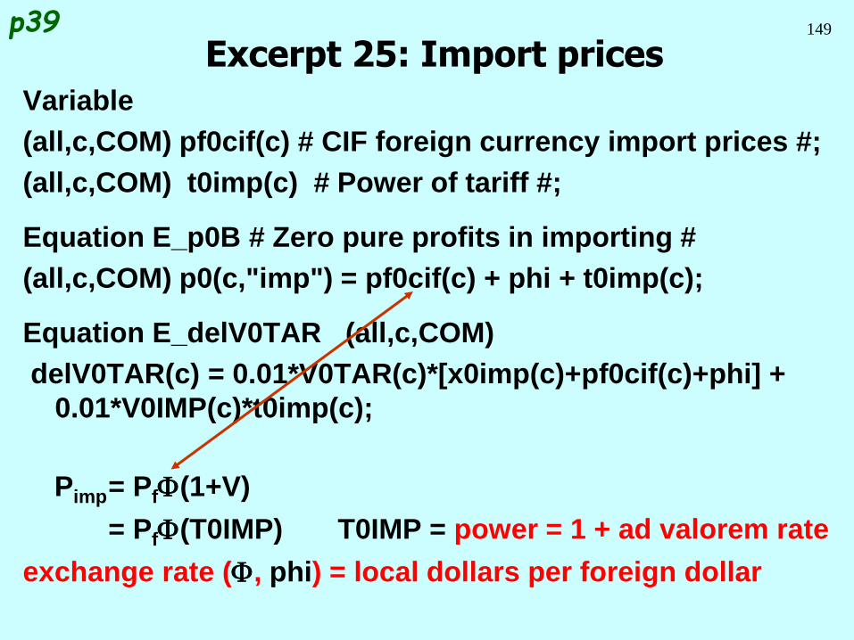
149
Variable
(all,c,COM) pf0cif(c) # CIF foreign currency import prices #;
(all,c,COM) t0imp(c) # Power of tariff #;
Equation E_p0B # Zero pure profits in importing #
(all,c,COM) p0(c,"imp") = pf0cif(c) + phi + t0imp(c);
Equation E_delV0TAR (all,c,COM)
delV0TAR(c) = 0.01*V0TAR(c)*[x0imp(c)+pf0cif(c)+phi] +
0.01*V0IMP(c)*t0imp(c);
Pimp= PfF(1+V)
= PfF(T0IMP) T0IMP = power = 1 + ad valorem rate
exchange rate (F, phi) = local dollars per foreign dollar
Excerpt 25: Import pricesp39
150
Progress so far . . .
Introduction Inventory demands
Database structure Margin demands
Solution method Market clearing
TABLO language Price equations
Production: input decisions Aggregates and indices
Production: output decisions Investment allocation
Investment: input decisions Labour market
Household demands Decompositions
Export demands Closure
Government demands Regional extension
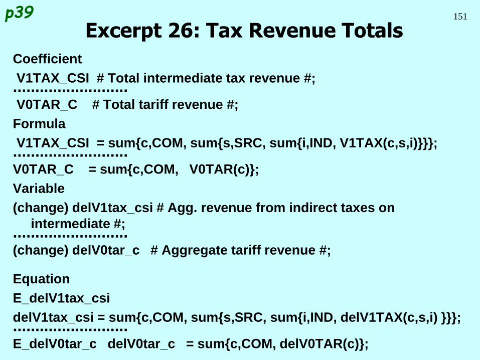
151
Coefficient
V1TAX_CSI # Total intermediate tax revenue #;..........................V0TAR_C # Total tariff revenue #;
Formula
V1TAX_CSI = sum{c,COM, sum{s,SRC, sum{i,IND, V1TAX(c,s,i)}}};..........................V0TAR_C = sum{c,COM, V0TAR(c)};
Variable
(change) delV1tax_csi # Agg. revenue from indirect taxes on
intermediate #;..........................(change) delV0tar_c # Aggregate tariff revenue #;
Equation
E_delV1tax_csi
delV1tax_csi = sum{c,COM, sum{s,SRC, sum{i,IND, delV1TAX(c,s,i) }}};..........................E_delV0tar_c delV0tar_c = sum{c,COM, delV0TAR(c)};
Excerpt 26: Tax Revenue Totalsp39
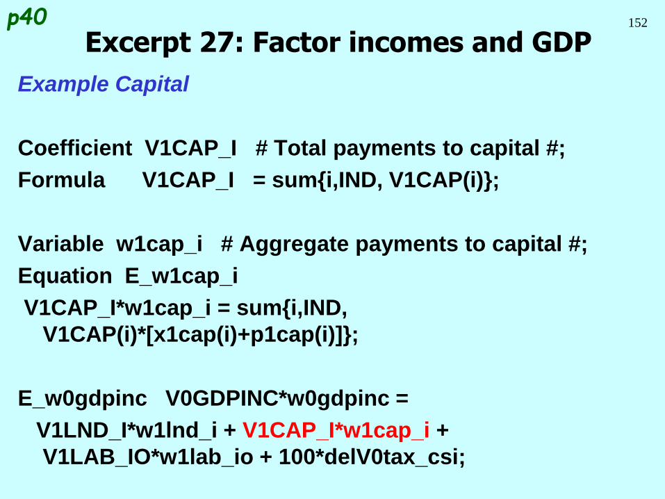
152
Example Capital
Coefficient V1CAP_I # Total payments to capital #;
Formula V1CAP_I = sum{i,IND, V1CAP(i)};
Variable w1cap_i # Aggregate payments to capital #;
Equation E_w1cap_i
V1CAP_I*w1cap_i = sum{i,IND,
V1CAP(i)*[x1cap(i)+p1cap(i)]};
E_w0gdpinc V0GDPINC*w0gdpinc =
V1LND_I*w1lnd_i + V1CAP_I*w1cap_i +
V1LAB_IO*w1lab_io + 100*delV0tax_csi;
Excerpt 27: Factor incomes and GDPp40
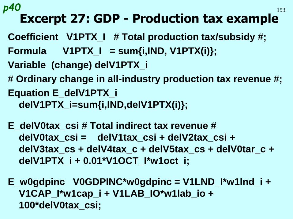
153
Coefficient V1PTX_I # Total production tax/subsidy #;
Formula V1PTX_I = sum{i,IND, V1PTX(i)};
Variable (change) delV1PTX_i
# Ordinary change in all-industry production tax revenue #;
Equation E_delV1PTX_i
delV1PTX_i=sum{i,IND,delV1PTX(i)};
E_delV0tax_csi # Total indirect tax revenue #
delV0tax_csi = delV1tax_csi + delV2tax_csi +
delV3tax_cs + delV4tax_c + delV5tax_cs + delV0tar_c +
delV1PTX_i + 0.01*V1OCT_I*w1oct_i;
E_w0gdpinc V0GDPINC*w0gdpinc = V1LND_I*w1lnd_i +
V1CAP_I*w1cap_i + V1LAB_IO*w1lab_io +
100*delV0tax_csi;
Excerpt 27: GDP - Production tax examplep40

154
Coefficient ! Expenditure Aggregates at Purchaser's Prices !
(all,c,COM) V0CIF(c) # Total ex-duty imports of good c #;
V0CIF_C # Total local currency import costs, excluding tariffs #;
V0IMP_C # Total basic-value imports (includes tariffs) #;
V2TOT_I # Total investment usage #;. . . . . . . . . . . . . . . .
V0GDPEXP # Nominal GDP from expenditure side #;
Formula
(all,c,COM) V0CIF(c) = V0IMP(c) - V0TAR(c);
V0CIF_C = sum{c,COM, V0CIF(c)};
V0IMP_C = sum{c,COM, V0IMP(c)};
V2TOT_I = sum{i,IND, V2TOT(i)};
V4TOT = sum{c,COM, V4PUR(c)};
V5TOT = sum{c,COM, sum{s,SRC, V5PUR(c,s)}};
V6TOT = sum{c,COM, sum{s,SRC, V6BAS(c,s)}};
V0GDPEXP = V3TOT + V2TOT_I + V5TOT + V6TOT + V4TOT - V0CIF_C;
Excerpt 28a: GDP expenditure aggregatesp41
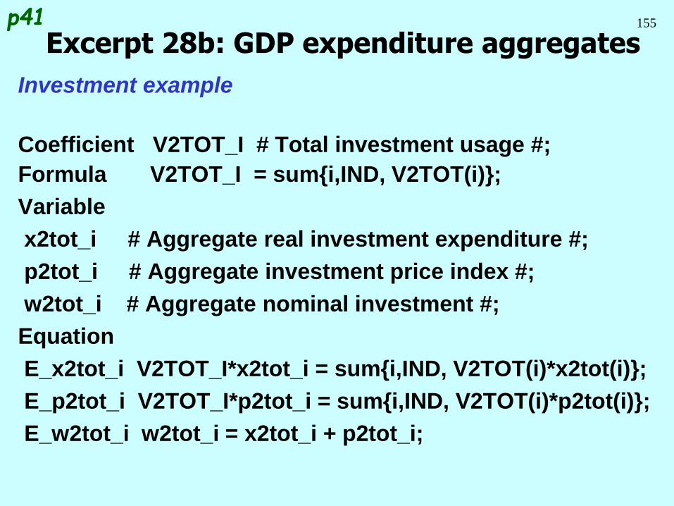
155
Investment example
Coefficient V2TOT_I # Total investment usage #;
Formula V2TOT_I = sum{i,IND, V2TOT(i)};
Variable
x2tot_i # Aggregate real investment expenditure #;
p2tot_i # Aggregate investment price index #;
w2tot_i # Aggregate nominal investment #;
Equation
E_x2tot_i V2TOT_I*x2tot_i = sum{i,IND, V2TOT(i)*x2tot(i)};
E_p2tot_i V2TOT_I*p2tot_i = sum{i,IND, V2TOT(i)*p2tot(i)};
E_w2tot_i w2tot_i = x2tot_i + p2tot_i;
Excerpt 28b: GDP expenditure aggregatesp41
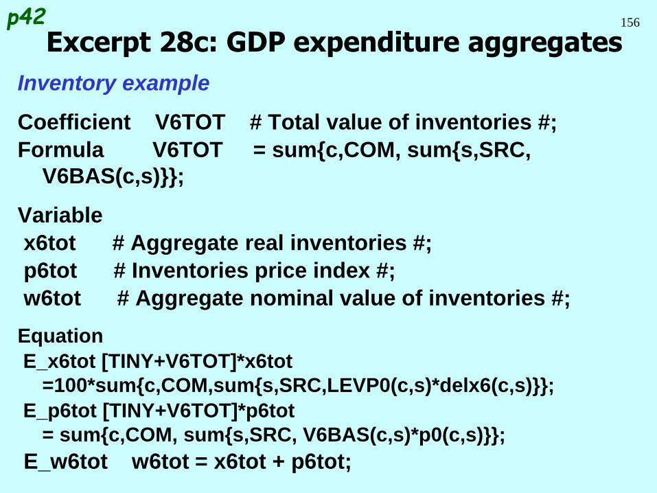
156
Inventory example
Coefficient V6TOT # Total value of inventories #;
Formula V6TOT = sum{c,COM, sum{s,SRC,
V6BAS(c,s)}};
Variable
x6tot # Aggregate real inventories #;
p6tot # Inventories price index #;
w6tot # Aggregate nominal value of inventories #;
Equation
E_x6tot [TINY+V6TOT]*x6tot
=100*sum{c,COM,sum{s,SRC,LEVP0(c,s)*delx6(c,s)}};
E_p6tot [TINY+V6TOT]*p6tot
= sum{c,COM, sum{s,SRC, V6BAS(c,s)*p0(c,s)}};
E_w6tot w6tot = x6tot + p6tot;
Excerpt 28c: GDP expenditure aggregatesp42
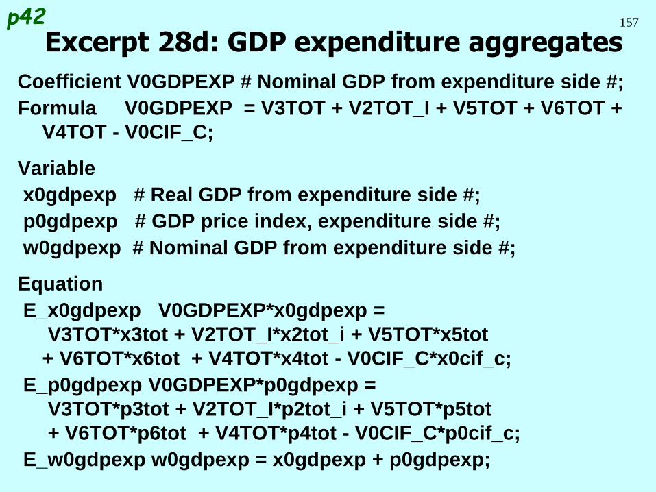
157
Coefficient V0GDPEXP # Nominal GDP from expenditure side #;
Formula V0GDPEXP = V3TOT + V2TOT_I + V5TOT + V6TOT +
V4TOT - V0CIF_C;
Variable
x0gdpexp # Real GDP from expenditure side #;
p0gdpexp # GDP price index, expenditure side #;
w0gdpexp # Nominal GDP from expenditure side #;
Equation
E_x0gdpexp V0GDPEXP*x0gdpexp =
V3TOT*x3tot + V2TOT_I*x2tot_i + V5TOT*x5tot
+ V6TOT*x6tot + V4TOT*x4tot - V0CIF_C*x0cif_c;
E_p0gdpexp V0GDPEXP*p0gdpexp =
V3TOT*p3tot + V2TOT_I*p2tot_i + V5TOT*p5tot
+ V6TOT*p6tot + V4TOT*p4tot - V0CIF_C*p0cif_c;
E_w0gdpexp w0gdpexp = x0gdpexp + p0gdpexp;
Excerpt 28d: GDP expenditure aggregatesp42
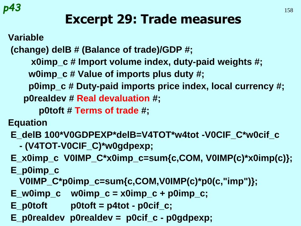
158
Variable
(change) delB # (Balance of trade)/GDP #;
x0imp_c # Import volume index, duty-paid weights #;
w0imp_c # Value of imports plus duty #;
p0imp_c # Duty-paid imports price index, local currency #;
p0realdev # Real devaluation #;
p0toft # Terms of trade #;
Equation
E_delB 100*V0GDPEXP*delB=V4TOT*w4tot -V0CIF_C*w0cif_c
- (V4TOT-V0CIF_C)*w0gdpexp;
E_x0imp_c V0IMP_C*x0imp_c=sum{c,COM, V0IMP(c)*x0imp(c)};
E_p0imp_c
V0IMP_C*p0imp_c=sum{c,COM,V0IMP(c)*p0(c,"imp")};
E_w0imp_c w0imp_c = x0imp_c + p0imp_c;
E_p0toft p0toft = p4tot - p0cif_c;
E_p0realdev p0realdev = p0cif_c - p0gdpexp;
Excerpt 29: Trade measuresp43
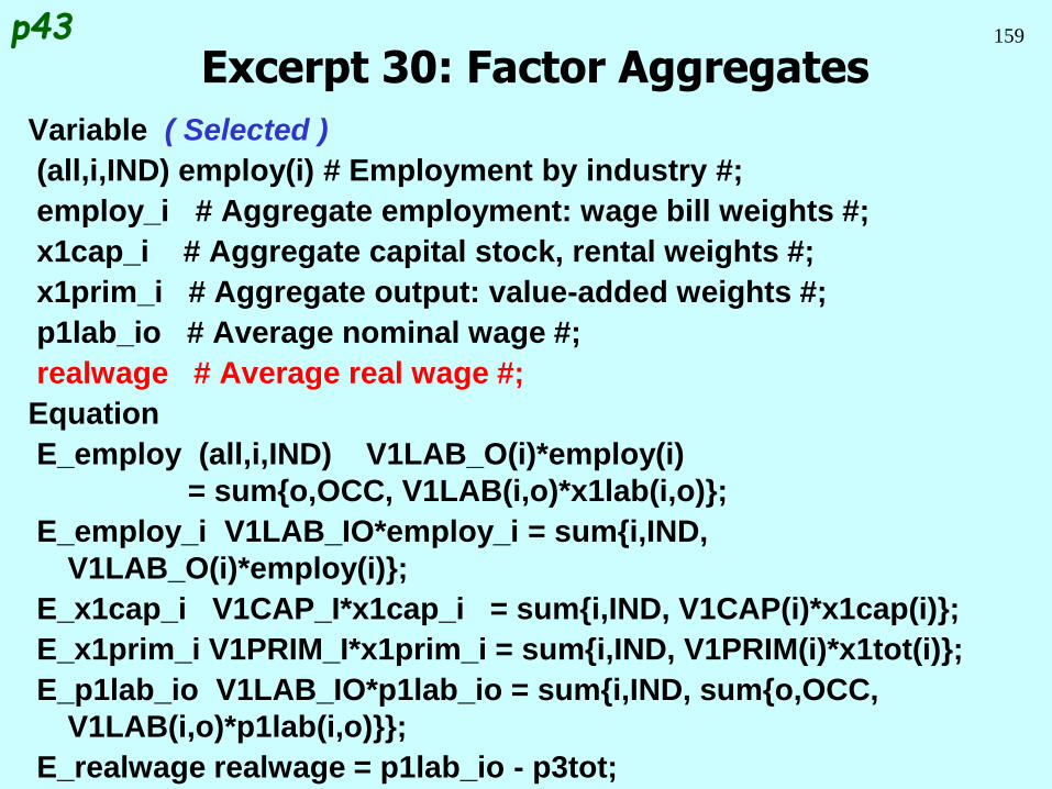
159
Variable ( Selected )
(all,i,IND) employ(i) # Employment by industry #;
employ_i # Aggregate employment: wage bill weights #;
x1cap_i # Aggregate capital stock, rental weights #;
x1prim_i # Aggregate output: value-added weights #;
p1lab_io # Average nominal wage #;
realwage # Average real wage #;
Equation
E_employ (all,i,IND) V1LAB_O(i)*employ(i)
= sum{o,OCC, V1LAB(i,o)*x1lab(i,o)};
E_employ_i V1LAB_IO*employ_i = sum{i,IND,
V1LAB_O(i)*employ(i)};
E_x1cap_i V1CAP_I*x1cap_i = sum{i,IND, V1CAP(i)*x1cap(i)};
E_x1prim_i V1PRIM_I*x1prim_i = sum{i,IND, V1PRIM(i)*x1tot(i)};
E_p1lab_io V1LAB_IO*p1lab_io = sum{i,IND, sum{o,OCC,
V1LAB(i,o)*p1lab(i,o)}};
E_realwage realwage = p1lab_io - p3tot;
Excerpt 30: Factor Aggregatesp43
160
Progress so far . . .
Introduction Inventory demands
Database structure Margin demands
Solution method Market clearing
TABLO language Price equations
Production: input decisions Aggregates and indices
Production: output decisions Investment allocation
Investment: input decisions Labour market
Household demands Decompositions
Export demands Closure
Government demands Regional extension
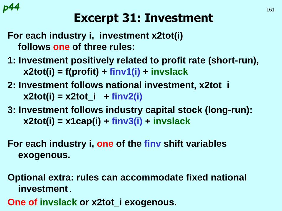
161
For each industry i, investment x2tot(i)
follows one of three rules:
1: Investment positively related to profit rate (short-run),
x2tot(i) = f(profit) + finv1(i) + invslack
2: Investment follows national investment, x2tot_i
x2tot(i) = x2tot_i + finv2(i)
3: Investment follows industry capital stock (long-run):
x2tot(i) = x1cap(i) + finv3(i) + invslack
For each industry i, one of the finv shift variables
exogenous.
Optional extra: rules can accommodate fixed national
investment .
One of invslack or x2tot_i exogenous.
Excerpt 31: Investmentp44
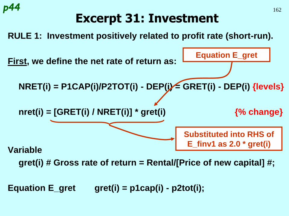
162
RULE 1: Investment positively related to profit rate (short-run).
First, we define the net rate of return as:
NRET(i) = P1CAP(i)/P2TOT(i) - DEP(i) = GRET(i) - DEP(i) {levels}
nret(i) = [GRET(i) / NRET(i)] * gret(i) {% change}
Variable
gret(i) # Gross rate of return = Rental/[Price of new capital] #;
Equation E_gret gret(i) = p1cap(i) - p2tot(i);
Excerpt 31: Investmentp44
Equation E_gret
Substituted into RHS of
E_finv1 as 2.0 * gret(i)
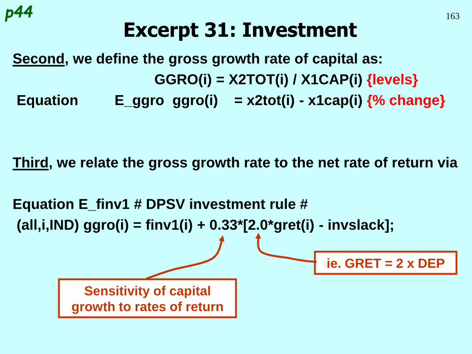
163
Second, we define the gross growth rate of capital as:
GGRO(i) = X2TOT(i) / X1CAP(i) {levels}
Equation E_ggro ggro(i) = x2tot(i) - x1cap(i) {% change}
Third, we relate the gross growth rate to the net rate of return via
Equation E_finv1 # DPSV investment rule #
(all,i,IND) ggro(i) = finv1(i) + 0.33*[2.0*gret(i) - invslack];
Excerpt 31: Investmentp44
Sensitivity of capital
growth to rates of return
ie. GRET = 2 x DEP
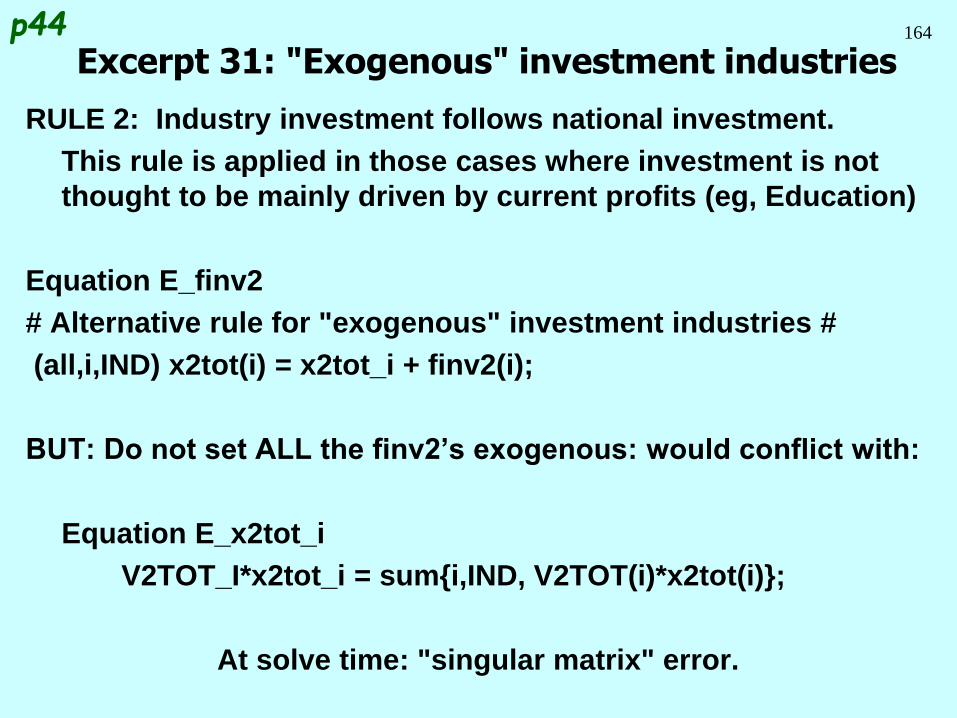
164
RULE 2: Industry investment follows national investment.
This rule is applied in those cases where investment is not
thought to be mainly driven by current profits (eg, Education)
Equation E_finv2
# Alternative rule for "exogenous" investment industries #
(all,i,IND) x2tot(i) = x2tot_i + finv2(i);
BUT: Do not set ALL the finv2’s exogenous: would conflict with:
Equation E_x2tot_i
V2TOT_I*x2tot_i = sum{i,IND, V2TOT(i)*x2tot(i)};
At solve time: "singular matrix" error.
Excerpt 31: "Exogenous" investment industriesp44
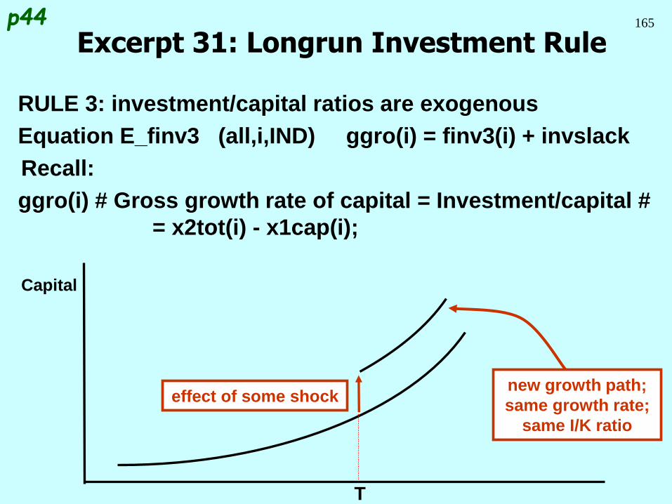
165
RULE 3: investment/capital ratios are exogenous
Equation E_finv3 (all,i,IND) ggro(i) = finv3(i) + invslack
Recall:
ggro(i) # Gross growth rate of capital = Investment/capital #
= x2tot(i) - x1cap(i);
Excerpt 31: Longrun Investment Rulep44
T
Capital
new growth path;
same growth rate;
same I/K ratio
effect of some shock
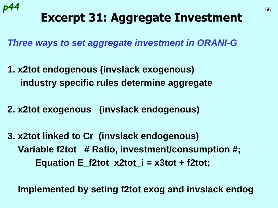
166
Three ways to set aggregate investment in ORANI-G
1. x2tot endogenous (invslack exogenous)
industry specific rules determine aggregate
2. x2tot exogenous (invslack endogenous)
3. x2tot linked to Cr (invslack endogenous)
Variable f2tot # Ratio, investment/consumption #;
Equation E_f2tot x2tot_i = x3tot + f2tot;
Implemented by seting f2tot exog and invslack endog
Excerpt 31: Aggregate Investmentp44
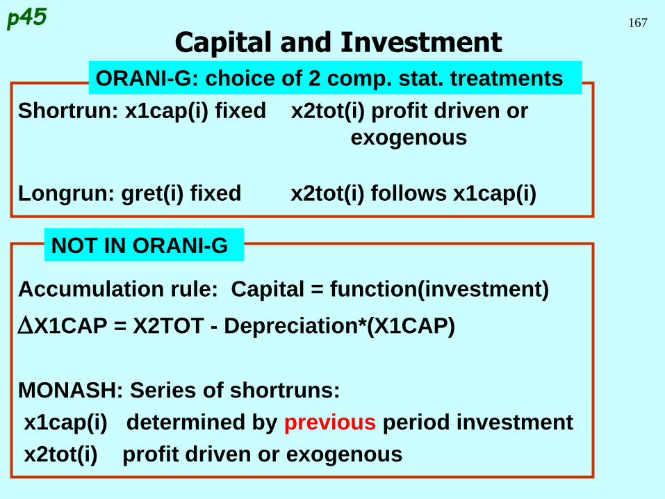
167
Shortrun: x1cap(i) fixed x2tot(i) profit driven or
exogenous
Longrun: gret(i) fixed x2tot(i) follows x1cap(i)
Accumulation rule: Capital = function(investment)
DX1CAP = X2TOT - Depreciation*(X1CAP)
MONASH: Series of shortruns:
x1cap(i) determined by previous period investment
x2tot(i) profit driven or exogenous
Capital and Investmentp45
NOT IN ORANI-G
ORANI-G: choice of 2 comp. stat. treatments
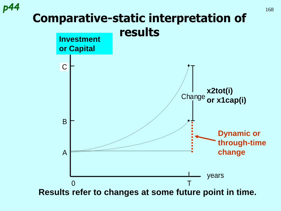
168
Comparative-static interpretation of results
Results refer to changes at some future point in time.
Employment
0 T
Change
A
years
B
C
p44
Investment
or Capital
x2tot(i)
or x1cap(i)
Dynamic or
through-time
change
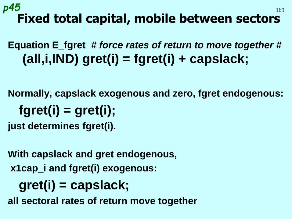
169
Equation E_fgret # force rates of return to move together #
(all,i,IND) gret(i) = fgret(i) + capslack;
Normally, capslack exogenous and zero, fgret endogenous:
fgret(i) = gret(i);just determines fgret(i).
With capslack and gret endogenous,
x1cap_i and fgret(i) exogenous:
gret(i) = capslack;all sectoral rates of return move together
Fixed total capital, mobile between sectorsp45
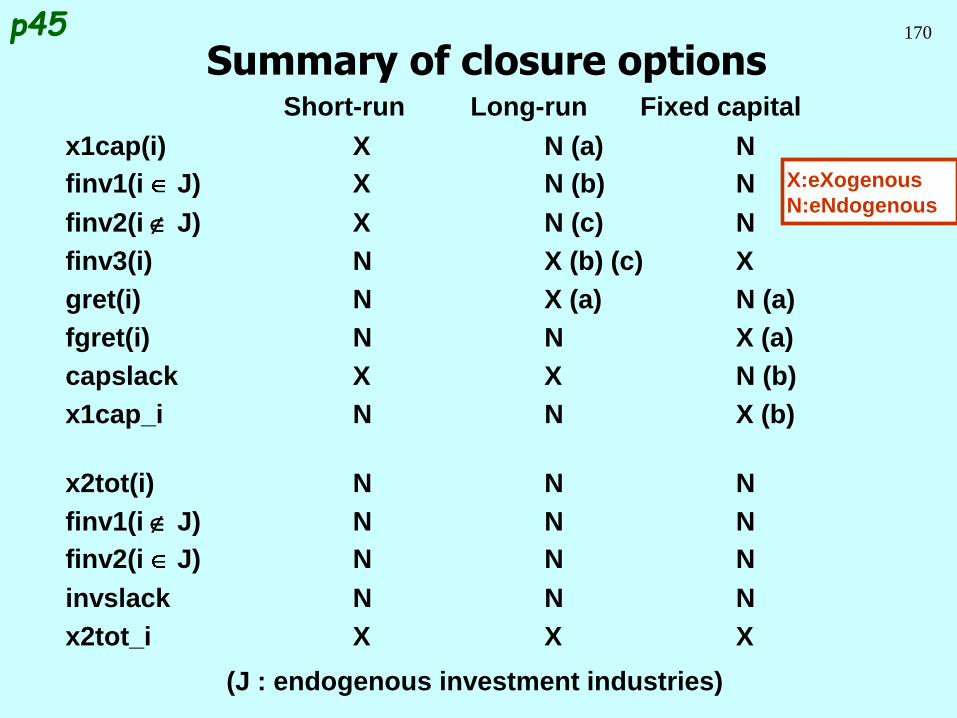
170
Short-run Long-run Fixed capital
x1cap(i) X N (a) N
finv1(i J) X N (b) N
finv2(i J) X N (c) N
finv3(i) N X (b) (c) X
gret(i) N X (a) N (a)
fgret(i) N N X (a)
capslack X X N (b)
x1cap_i N N X (b)
x2tot(i) N N N
finv1(i J) N N N
finv2(i J) N N N
invslack N N N
x2tot_i X X X
(J : endogenous investment industries)
Summary of closure optionsp45
X:eXogenous
N:eNdogenous
171
Progress so far . . .
Introduction Inventory demands
Database structure Margin demands
Solution method Market clearing
TABLO language Price equations
Production: input decisions Aggregates and indices
Production: output decisions Investment allocation
Investment: input decisions Labour market
Household demands Decompositions
Export demands Closure
Government demands Regional extension
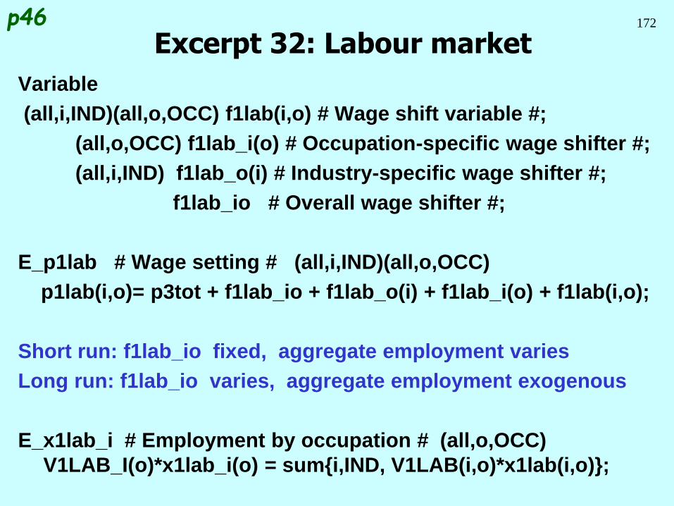
172
Variable
(all,i,IND)(all,o,OCC) f1lab(i,o) # Wage shift variable #;
(all,o,OCC) f1lab_i(o) # Occupation-specific wage shifter #;
(all,i,IND) f1lab_o(i) # Industry-specific wage shifter #;
f1lab_io # Overall wage shifter #;
E_p1lab # Wage setting # (all,i,IND)(all,o,OCC)
p1lab(i,o)= p3tot + f1lab_io + f1lab_o(i) + f1lab_i(o) + f1lab(i,o);
Short run: f1lab_io fixed, aggregate employment varies
Long run: f1lab_io varies, aggregate employment exogenous
E_x1lab_i # Employment by occupation # (all,o,OCC)
V1LAB_I(o)*x1lab_i(o) = sum{i,IND, V1LAB(i,o)*x1lab(i,o)};
Excerpt 32: Labour marketp46
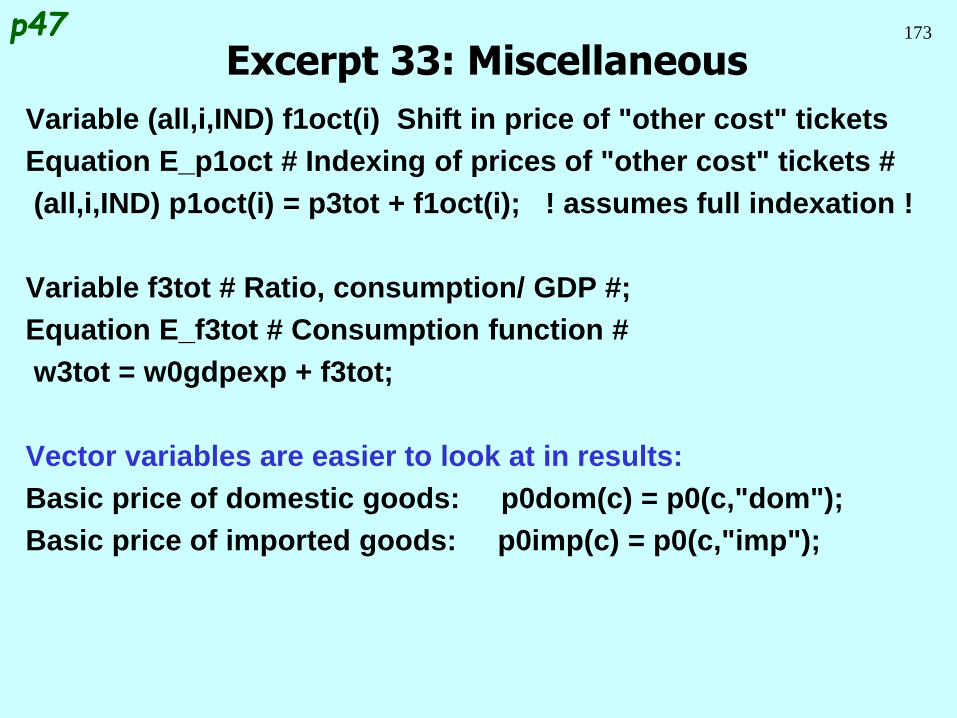
173
Variable (all,i,IND) f1oct(i) Shift in price of "other cost" tickets
Equation E_p1oct # Indexing of prices of "other cost" tickets #
(all,i,IND) p1oct(i) = p3tot + f1oct(i); ! assumes full indexation !
Variable f3tot # Ratio, consumption/ GDP #;
Equation E_f3tot # Consumption function #
w3tot = w0gdpexp + f3tot;
Vector variables are easier to look at in results:
Basic price of domestic goods: p0dom(c) = p0(c,"dom");
Basic price of imported goods: p0imp(c) = p0(c,"imp");
Excerpt 33: Miscellaneousp47
174
Progress so far . . .
Introduction Inventory demands
Database structure Margin demands
Solution method Market clearing
TABLO language Price equations
Production: input decisions Aggregates and indices
Production: output decisions Investment allocation
Investment: input decisions Labour market
Household demands Decompositions
Export demands Closure
Government demands Regional extension
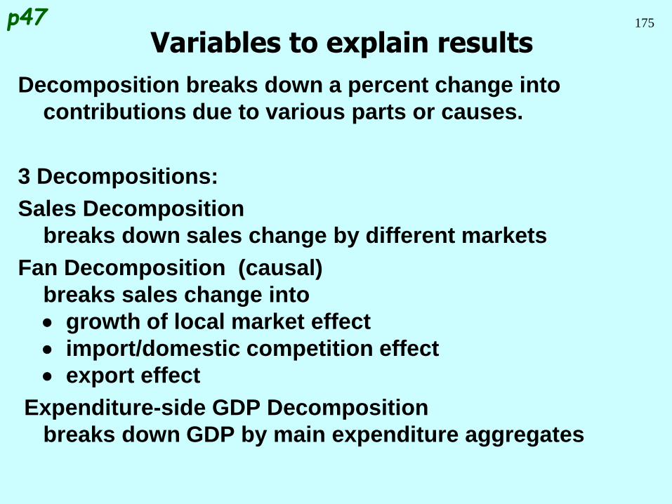
175
Decomposition breaks down a percent change into
contributions due to various parts or causes.
3 Decompositions:
Sales Decomposition
breaks down sales change by different markets
Fan Decomposition (causal)
breaks sales change into
growth of local market effect
import/domestic competition effect
export effect
Expenditure-side GDP Decomposition
breaks down GDP by main expenditure aggregates
Variables to explain resultsp47
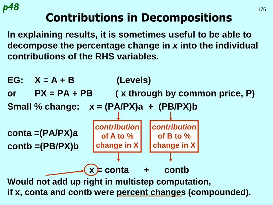
176
In explaining results, it is sometimes useful to be able to
decompose the percentage change in x into the individual
contributions of the RHS variables.
EG: X = A + B (Levels)
or PX = PA + PB ( x through by common price, P)
Small % change: x = (PA/PX)a + (PB/PX)b
conta =(PA/PX)a
contb =(PB/PX)b
x = conta + contb
Would not add up right in multistep computation,
if x, conta and contb were percent changes (compounded).
Contributions in Decompositionsp48
contribution
of A to %
change in X
contribution
of B to %
change in X
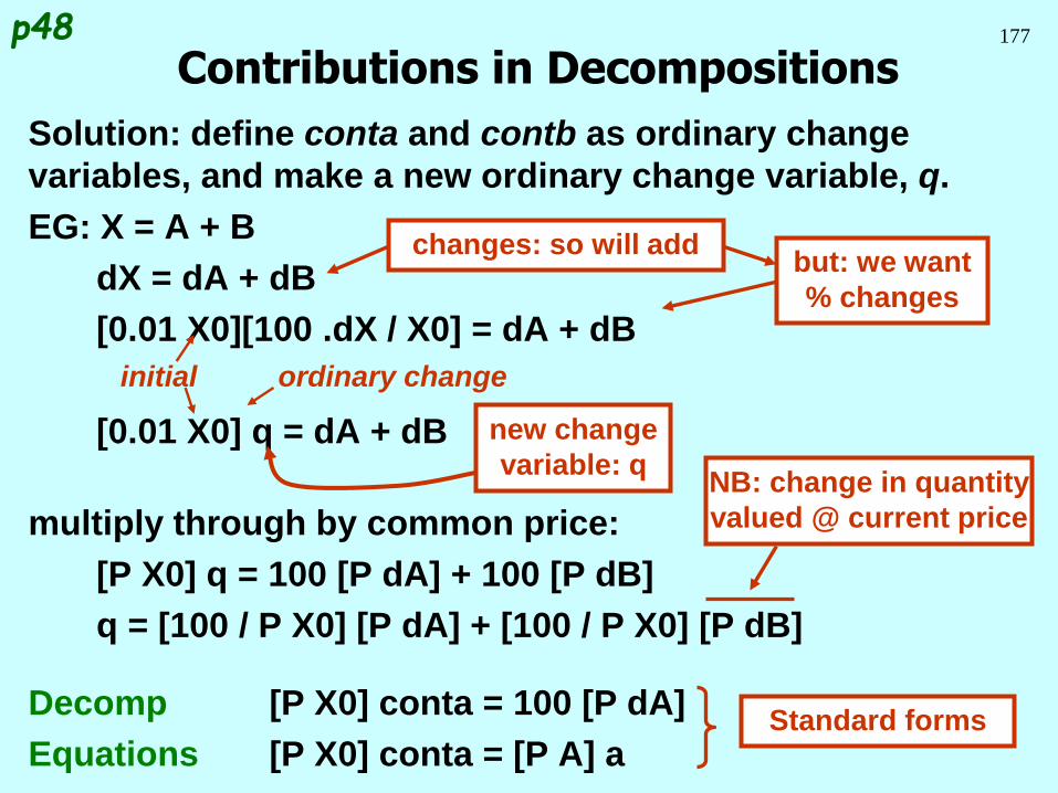
177
Solution: define conta and contb as ordinary change
variables, and make a new ordinary change variable, q.
EG: X = A + B
dX = dA + dB
[0.01 X0][100 .dX / X0] = dA + dB
[0.01 X0] q = dA + dB
multiply through by common price:
[P X0] q = 100 [P dA] + 100 [P dB]
q = [100 / P X0] [P dA] + [100 / P X0] [P dB]
Decomp [P X0] conta = 100 [P dA]
Equations [P X0] conta = [P A] a
Contributions in Decompositionsp48
initial ordinary change
changes: so will addbut: we want
% changes
new change
variable: qNB: change in quantity
valued @ current price
Standard forms
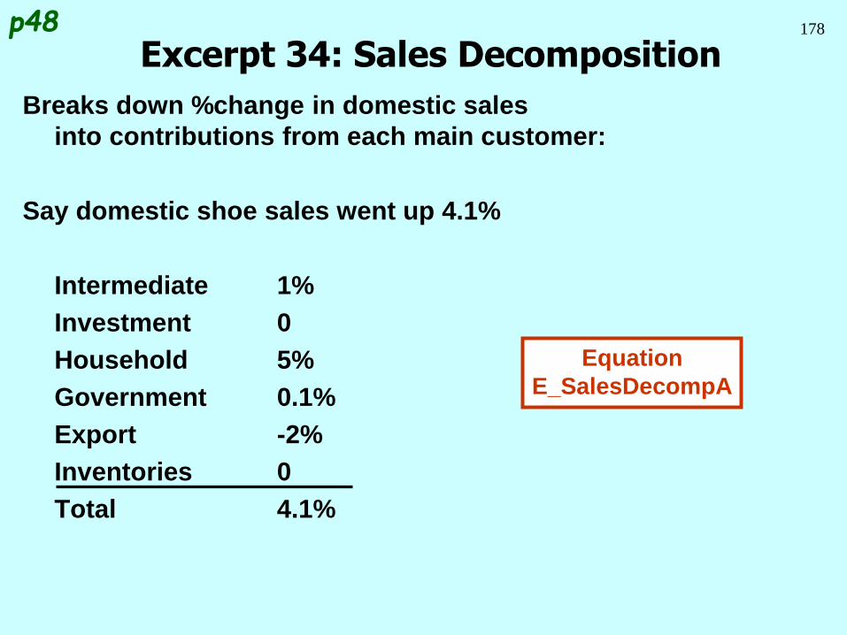
178
Breaks down %change in domestic sales
into contributions from each main customer:
Say domestic shoe sales went up 4.1%
Intermediate 1%
Investment 0
Household 5%
Government 0.1%
Export -2%
Inventories 0
Total 4.1%
Excerpt 34: Sales Decompositionp48
Equation
E_SalesDecompA
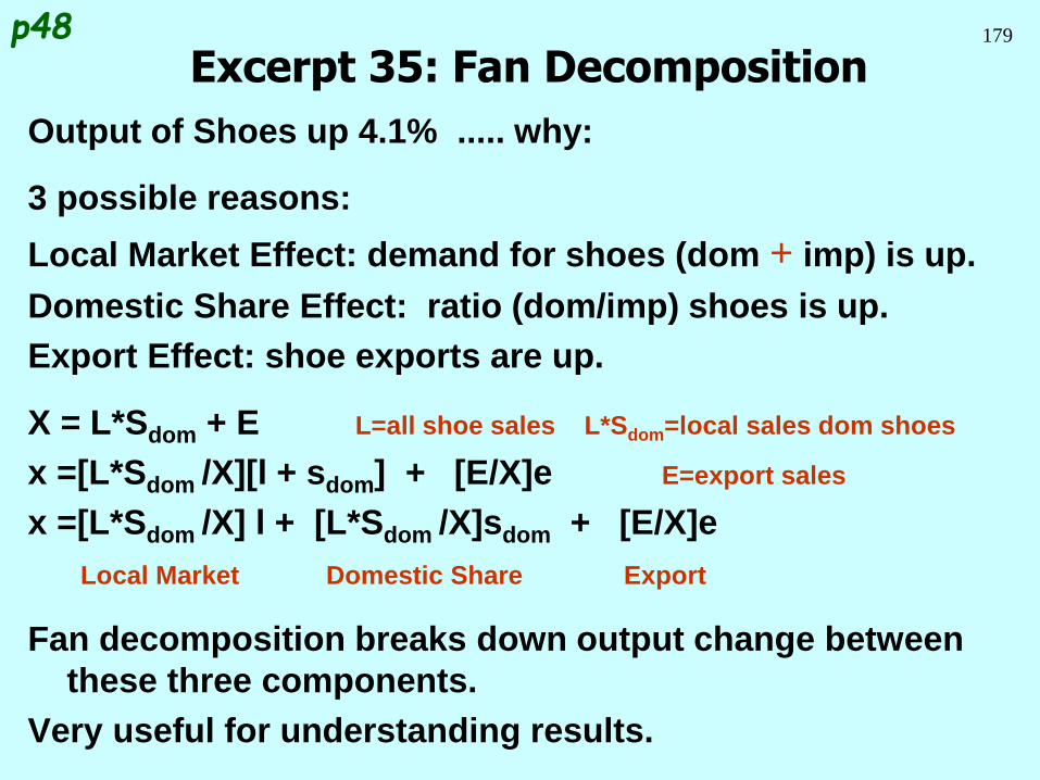
179
Output of Shoes up 4.1% ..... why:
3 possible reasons:
Local Market Effect: demand for shoes (dom + imp) is up.
Domestic Share Effect: ratio (dom/imp) shoes is up.
Export Effect: shoe exports are up.
X = L*Sdom + E L=all shoe sales L*Sdom=local sales dom shoes
x =[L*Sdom /X][l + sdom] + [E/X]e E=export sales
x =[L*Sdom /X] l + [L*Sdom /X]sdom + [E/X]e
Local Market Domestic Share Export
Fan decomposition breaks down output change between
these three components.
Very useful for understanding results.
Excerpt 35: Fan Decompositionp48
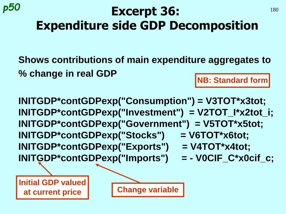
180
Shows contributions of main expenditure aggregates to
% change in real GDP
INITGDP*contGDPexp("Consumption") = V3TOT*x3tot;
INITGDP*contGDPexp("Investment") = V2TOT_I*x2tot_i;
INITGDP*contGDPexp("Government") = V5TOT*x5tot;
INITGDP*contGDPexp("Stocks") = V6TOT*x6tot;
INITGDP*contGDPexp("Exports") = V4TOT*x4tot;
INITGDP*contGDPexp("Imports") = - V0CIF_C*x0cif_c;
Excerpt 36:Expenditure side GDP Decomposition
p50
NB: Standard form
Change variableInitial GDP valued
at current price
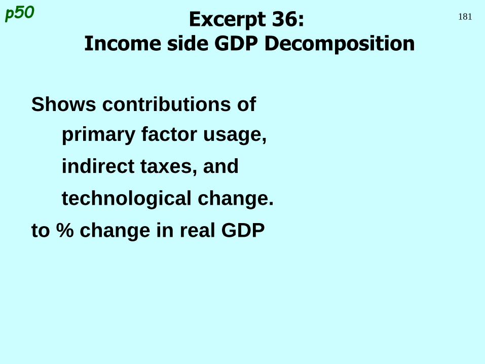
181
Shows contributions of
primary factor usage,
indirect taxes, and
technological change.
to % change in real GDP
Excerpt 36:Income side GDP Decomposition
p50
182
Many useful aggregates
Excerpt 37 -42: The Summary filep51-53

183
covered in a later lecture
Regional Extensionp55
184
Progress so far . . .
Introduction Inventory demands
Database structure Margin demands
Solution method Market clearing
TABLO language Price equations
Production: input decisions Aggregates and indices
Production: output decisions Investment allocation
Investment: input decisions Labour market
Household demands Decompositions
Export demands Closure
Government demands Regional extension
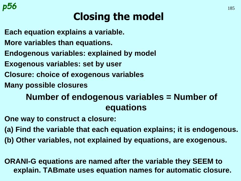
185
Closing the model
Each equation explains a variable.
More variables than equations.
Endogenous variables: explained by model
Exogenous variables: set by user
Closure: choice of exogenous variables
Many possible closures
Number of endogenous variables = Number of
equations
One way to construct a closure:
(a) Find the variable that each equation explains; it is endogenous.
(b) Other variables, not explained by equations, are exogenous.
ORANI-G equations are named after the variable they SEEM to
explain. TABmate uses equation names for automatic closure.
p56
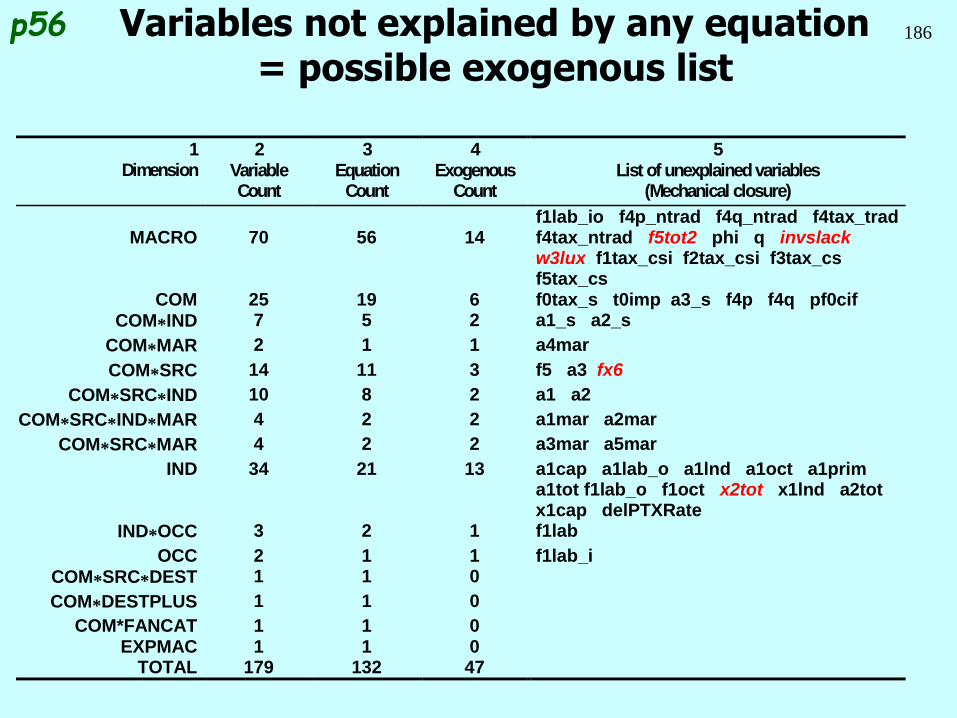
186Variables not explained by any equation= possible exogenous list
p56
1Dimension
2VariableCount
3Equation
Count
4Exogenous
Count
5List of unexplained variables
(Mechanical closure)
MACRO 70 56 14f1lab_io f4p_ntrad f4q_ntrad f4tax_tradf4tax_ntrad f5tot2 phi q invslack w3lux f1tax_csi f2tax_csi f3tax_csf5tax_cs
COM 25 19 6 f0tax_s t0imp a3_s f4p f4q pf0cifCOM*IND 7 5 2 a1_s a2_s
COM*MAR 2 1 1 a4mar
COM*SRC 14 11 3 f5 a3 fx6
COM*SRC*IND 10 8 2 a1 a2
COM*SRC*IND*MAR 4 2 2 a1mar a2mar
COM*SRC*MAR 4 2 2 a3mar a5mar
IND 34 21 13 a1cap a1lab_o a1lnd a1oct a1prima1tot f1lab_o f1oct x2tot x1lnd a2totx1cap delPTXRate
IND*OCC 3 2 1 f1lab
OCC 2 1 1 f1lab_iCOM*SRC*DEST 1 1 0
COM*DESTPLUS 1 1 0
COM*FANCAT 1 1 0EXPMAC 1 1 0
TOTAL 179 132 47
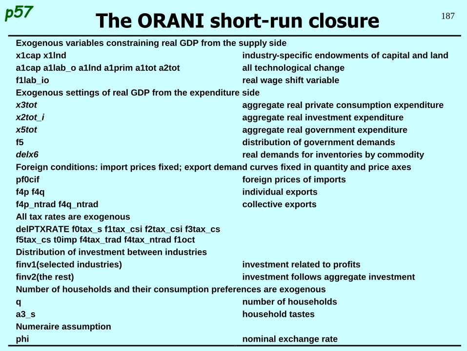
187The ORANI short-run closurep57
Exogenous variables constraining real GDP from the supply side
x1cap x1lnd industry-specific endowments of capital and land
a1cap a1lab_o a1lnd a1prim a1tot a2tot all technological change
f1lab_io real wage shift variable
Exogenous settings of real GDP from the expenditure side
x3tot aggregate real private consumption expenditure
x2tot_i aggregate real investment expenditure
x5tot aggregate real government expenditure
f5 distribution of government demands
delx6 real demands for inventories by commodity
Foreign conditions: import prices fixed; export demand curves fixed in quantity and price axes
pf0cif foreign prices of imports
f4p f4q individual exports
f4p_ntrad f4q_ntrad collective exports
All tax rates are exogenous
delPTXRATE f0tax_s f1tax_csi f2tax_csi f3tax_cs
f5tax_cs t0imp f4tax_trad f4tax_ntrad f1oct
Distribution of investment between industries
finv1(selected industries) investment related to profits
finv2(the rest) investment follows aggregate investment
Number of households and their consumption preferences are exogenous
q number of households
a3_s household tastes
Numeraire assumption
phi nominal exchange rate
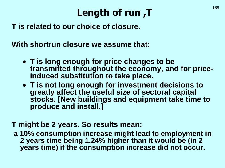
188
Length of run ,T
T is related to our choice of closure.
With shortrun closure we assume that:
T is long enough for price changes to be transmitted throughout the economy, and for price-induced substitution to take place.
T is not long enough for investment decisions to greatly affect the useful size of sectoral capital stocks. [New buildings and equipment take time to produce and install.]
T might be 2 years. So results mean:
a 10% consumption increase might lead to employment in 2 years time being 1.24% higher than it would be (in 2 years time) if the consumption increase did not occur.
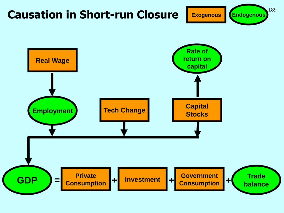
189
Causation in Short-run Closure
Private
ConsumptionInvestment
Government
Consumption
Real Wage
Capital
StocksTech Change
Rate of
return on
capital
Trade
balance
Employment
GDP = +++
EndogenousExogenous
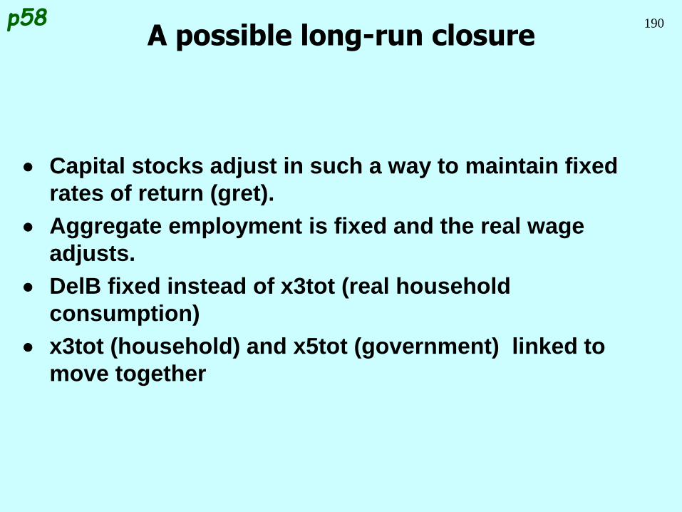
190
A possible long-run closure
Capital stocks adjust in such a way to maintain fixed
rates of return (gret).
Aggregate employment is fixed and the real wage
adjusts.
DelB fixed instead of x3tot (real household
consumption)
x3tot (household) and x5tot (government) linked to
move together
p58
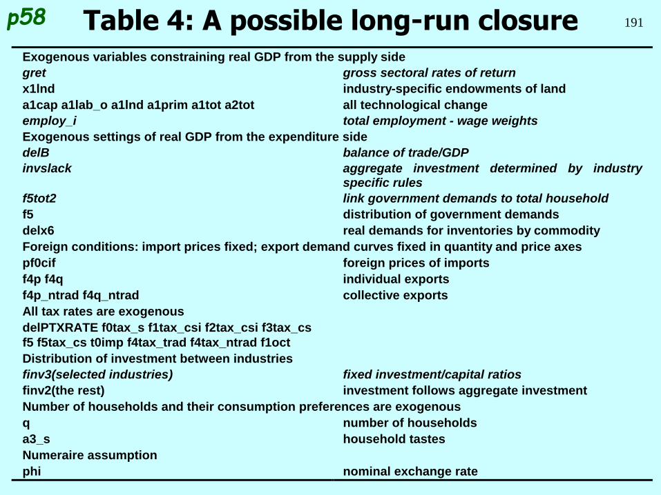
191Table 4: A possible long-run closurep58
Exogenous variables constraining real GDP from the supply side
gret gross sectoral rates of return
x1lnd industry-specific endowments of land
a1cap a1lab_o a1lnd a1prim a1tot a2tot all technological change
employ_i total employment - wage weights
Exogenous settings of real GDP from the expenditure side
delB balance of trade/GDP
invslack aggregate investment determined by industryspecific rules
f5tot2 link government demands to total household
f5 distribution of government demands
delx6 real demands for inventories by commodity
Foreign conditions: import prices fixed; export demand curves fixed in quantity and price axes
pf0cif foreign prices of imports
f4p f4q individual exports
f4p_ntrad f4q_ntrad collective exports
All tax rates are exogenous
delPTXRATE f0tax_s f1tax_csi f2tax_csi f3tax_cs
f5 f5tax_cs t0imp f4tax_trad f4tax_ntrad f1oct
Distribution of investment between industries
finv3(selected industries) fixed investment/capital ratios
finv2(the rest) investment follows aggregate investment
Number of households and their consumption preferences are exogenous
q number of households
a3_s household tastes
Numeraire assumption
phi nominal exchange rate
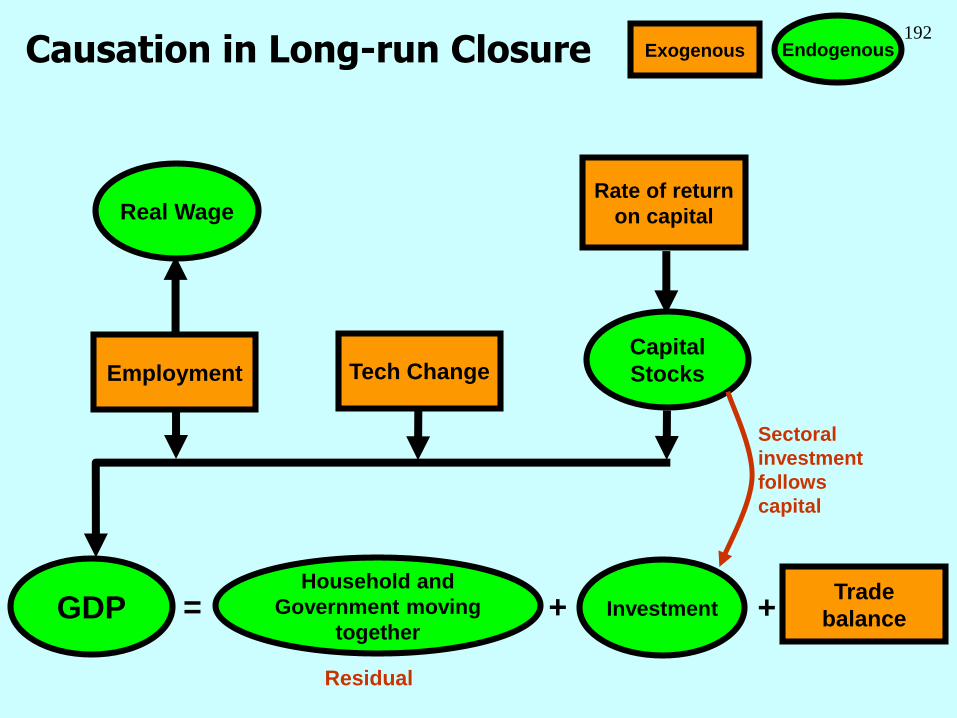
192
Causation in Long-run Closure
Trade
balance
Employment
Rate of return
on capital
Tech ChangeCapital
Stocks
Real Wage
GDP = ++
EndogenousExogenous
Investment
Household and
Government moving
together
Sectoral
investment
follows
capital
Residual
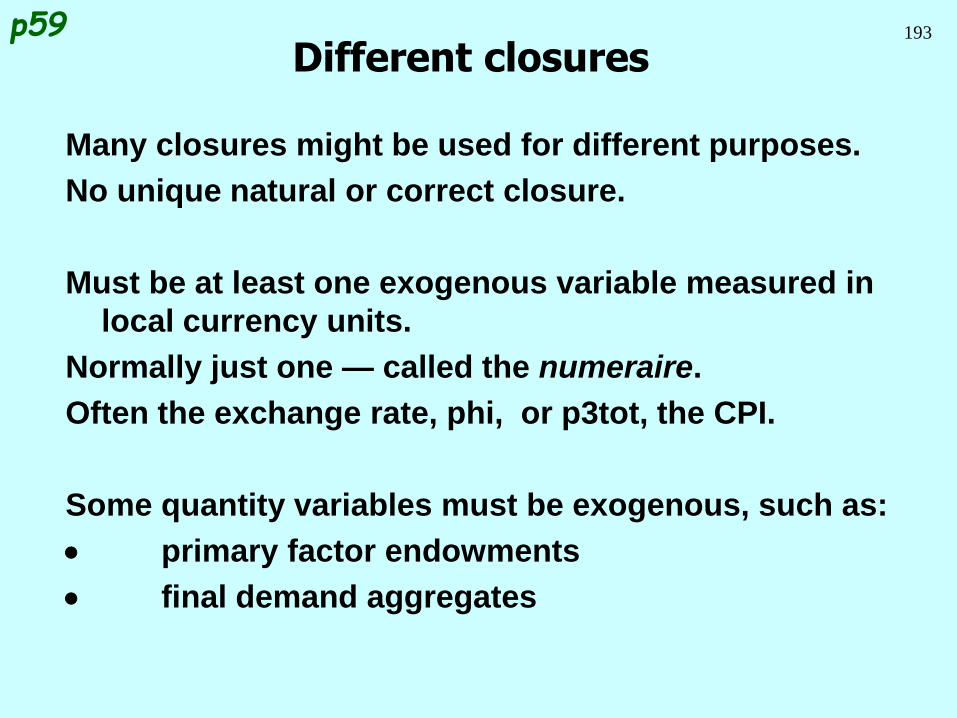
193
Different closures
Many closures might be used for different purposes.
No unique natural or correct closure.
Must be at least one exogenous variable measured in
local currency units.
Normally just one — called the numeraire.
Often the exchange rate, phi, or p3tot, the CPI.
Some quantity variables must be exogenous, such as:
primary factor endowments
final demand aggregates
p59

194
Three Macro Don't Knows
Absolute price level. Numeraire choice determines
whether changes in the real exchange rate appear
as changes in domestic prices or in changes in the
exchange rate. Real variables unaffected.
Labour supply. Closure determines whether labour
market changes appear as changes in either wage
or employment.
Size and composition of absorption. Either
exogenous or else adusting to accommodate fixed
trade balance. Closure determines how changes in
national income appear.
p59
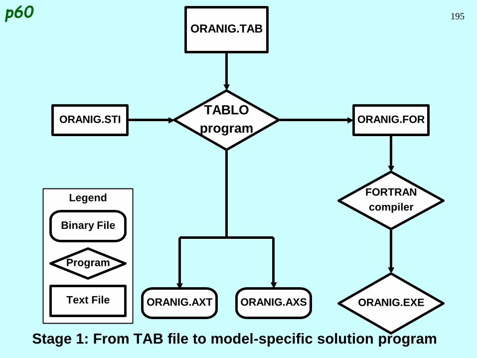
195
Stage 1: From TAB file to model-specific solution program
ORANIG.AXT ORANIG.AXS
ORANIG.FOR
ORANIG.TAB
ORANIG.EXE
Legend
Text File
Program
Binary File
FORTRAN
compiler
ORANIG.STITABLO
program
p60
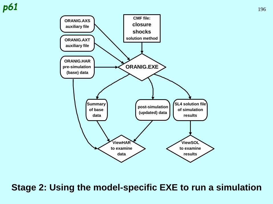
196
Stage 2: Using the model-specific EXE to run a simulation
ORANIG.AXT
auxiliary file
ORANIG.AXS
auxiliary file
ORANIG.EXE
CMF file:
closure
shocks
solution method
ORANIG.HAR
pre-simulation
(base) data
SL4 solution file
of simulation
results
Summary
of base
data
post-simulation
(updated) data
ViewHAR
to examine
data
ViewSOL
to examine
results
p61
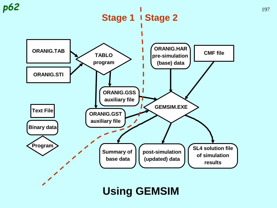
197
Using GEMSIM
ORANIG.GST
auxiliary file
ORANIG.GSS
auxiliary file
GEMSIM.EXE
CMF fileORANIG.HAR
pre-simulation
(base) data
SL4 solution file
of simulation
results
Summary of
base data
post-simulation
(updated) data
ORANIG.TAB
ORANIG.STI
TABLO
program
Binary data
Program
Text File
Stage 1 Stage 2p62

198
The End