Oracle® Strategic Network Optimization · document and if any concerns are already addressed. To...

Oracle® Strategic Network OptimizationImplementation GuideRelease 12.2Part No. E48785-01

September, 2013

Oracle Strategic Network Optimization Implementation Guide, Release 12.2

Part No. E48785-01

Copyright © 2013, Oracle and/or its affiliates. All rights reserved.

Primary Author: Kyle MacLean

Contributing Author: Alex Kim

Oracle and Java are registered trademarks of Oracle and/or its affiliates. Other names may be trademarks of their respective owners.

Intel and Intel Xeon are trademarks or registered trademarks of Intel Corporation. All SPARC trademarks are used under license and are trademarks or registered trademarks of SPARC International, Inc. AMD, Opteron, the AMD logo, and the AMD Opteron logo are trademarks or registered trademarks of Advanced Micro Devices. UNIX is a registered trademark of The Open Group.

This software and related documentation are provided under a license agreement containing restrictions on use and disclosure and are protected by intellectual property laws. Except as expressly permitted in your license agreement or allowed by law, you may not use, copy, reproduce, translate, broadcast, modify, license, transmit, distribute, exhibit, perform, publish, or display any part, in any form, or by any means. Reverse engineering, disassembly, or decompilation of this software, unless required by law for interoperability, is prohibited.

The information contained herein is subject to change without notice and is not warranted to be error-free. If you find any errors, please report them to us in writing.

If this is software or related documentation that is delivered to the U.S. Government or anyone licensing it on behalf of the U.S. Government, the following notice is applicable:

U.S. GOVERNMENT END USERS: Oracle programs, including any operating system, integrated software, any programs installed on the hardware, and/or documentation, delivered to U.S. Government end users are "commercial computer software" pursuant to the applicable Federal Acquisition Regulation and agency-specific supplemental regulations. As such, use, duplication, disclosure, modification, and adaptation of the programs, including any operating system, integrated software, any programs installed on the hardware, and/or documentation, shall be subject to license terms and license restrictions applicable to the programs. No other rights are granted to the U.S. Government.

This software or hardware is developed for general use in a variety of information management applications. It is not developed or intended for use in any inherently dangerous applications, including applications that may create a risk of personal injury. If you use this software or hardware in dangerous applications, then you shall be responsible to take all appropriate fail-safe, backup, redundancy, and other measures to ensure its safe use. Oracle Corporation and its affiliates disclaim any liability for any damages caused by use of this software or hardware in dangerous applications.

This software or hardware and documentation may provide access to or information on content, products, and services from third parties. Oracle Corporation and its affiliates are not responsible for and expressly disclaim all warranties of any kind with respect to third-party content, products, and services. Oracle Corporation and its affiliates will not be responsible for any loss, costs, or damages incurred due to your access to or use of third-party content, products, or services.

iii

Contents

Send Us Your Comments

Preface

1 Getting Started in Oracle Strategic Network OptimizationOracle Strategic Network Optimization Overview.................................................................. 1-1Oracle Strategic Network Optimization Business Processes................................................... 1-2Integration With Oracle Advanced Planning Suite..................................................................1-4Oracle Strategic Network Optimization Implementation....................................................... 1-4

2 Supply Chain Network Optimization OverviewIntroduction to Strategic Network Optimization..................................................................... 2-1Introduction to Models............................................................................................................. 2-2Optimal Model Solutions......................................................................................................... 2-4Solutions for Business Problems............................................................................................ 2-19

3 Building Supply Chain Network ModelsSupply Chain Network Models Overview............................................................................... 3-1Modeling Commodity Flows.................................................................................................... 3-6Time Periods............................................................................................................................ 3-11Organizing Models with Sets................................................................................................. 3-12Profit Models........................................................................................................................... 3-17Modeling Supply Chain Operations...................................................................................... 3-18Modeling Commodity Flows.................................................................................................. 3-22Commodity Groups................................................................................................................. 3-27Units of Measure..................................................................................................................... 3-31

iv

Creating, Renaming and Deleting Time Periods....................................................................3-37Period Group Levels and Period Groups................................................................................3-38Organizing Models Using Sets............................................................................................... 3-43Alerts........................................................................................................................................ 3-46

4 Working with ModelsModels Overview...................................................................................................................... 4-1Opening Models........................................................................................................................ 4-5The Model Workspace.............................................................................................................. 4-6Viewing Models in Flow View............................................................................................... 4-12Viewing Models in Map View................................................................................................4-20Saving Models......................................................................................................................... 4-30Selecting and Unselecting Nodes, Arcs and Commodities.................................................... 4-31Exporting Nodes and Arcs in .imp Format............................................................................. 4-36

5 Viewing and Entering Supply Chain DataSupply Chain Data Overview................................................................................................... 5-1Opening Data in Nodes and Arcs............................................................................................. 5-6Entering Supply Chain Data................................................................................................... 5-10Hiding and Showing Fields in Properties Windows............................................................. 5-12

6 Working with the Currency TableCurrency Table Overview......................................................................................................... 6-1Defining Currency Rates......................................................................................................... 6-10Defining Currency in Nodes and Arcs................................................................................... 6-14Exporting Currency Values Using Smarts.............................................................................. 6-15

7 Mitigating Risk in Supply Chain ModelsRisk Mitigation Overview........................................................................................................ 7-1The Risk Registry...................................................................................................................... 7-4Defining Risk in Batch Mode................................................................................................... 7-6Solving Models with Risk Adjusted Costs...............................................................................7-7

8 Scenarios, Events, and Key Performance IndicatorsScenarios and Events Overview................................................................................................ 8-1Working with Scenarios and Events......................................................................................... 8-4Key Performance Overview...................................................................................................... 8-7

v

9 Solving ModelsSolving Models Overview........................................................................................................ 9-1Solving Models........................................................................................................................9-12Viewing Solve Results............................................................................................................ 9-13Capital Asset Management Solves..........................................................................................9-15Working with Solves............................................................................................................... 9-17Infeasible Solves..................................................................................................................... 9-21Adjusting Solver Tuning Parameters..................................................................................... 9-24

10 Finding or Replacing DataFind and Replace Overview.................................................................................................... 10-1Performing a Find.................................................................................................................... 10-6Performing a Replace.............................................................................................................. 10-7

11 Reporting and Extracting DataReporting and Extracting Data Overview...............................................................................11-1Extracting Data Using Report Queries.................................................................................... 11-5Organizing Report Queries Using Groups........................................................................... 11-10Report Overrides................................................................................................................... 11-11Extracting Data Using Commands........................................................................................ 11-19Working with Publishing Profiles........................................................................................ 11-24

12 Using the Data EditorData Editor Overview.............................................................................................................. 12-1Configuring Data Editor Views.............................................................................................. 12-2Saving, Loading and Deleting Views in the Data Editor....................................................... 12-9Changing All Values in Rows, Columns or Views.............................................................. 12-10Exporting Data from the Data Editor.................................................................................... 12-11Performing Calculations on Data..........................................................................................12-12Highlighting Data................................................................................................................. 12-16Arithmetic Symbols and Functions...................................................................................... 12-20

13 Automating Processes Using Import and Batch CommandsUpdating Models by Importing Files..................................................................................... 13-1Importing Files...................................................................................................................... 13-12Automating Processes Using Batch Mode............................................................................ 13-13Running Batch Scripts or Batch Commands.........................................................................13-21

vi

14 Customizing Menus and HelpCreating Customized Menus.................................................................................................. 14-1

A Appendix ANode Reference......................................................................................................................... A-1

B Appendix BArc Fields and Symbolic Tags.................................................................................................. B-1

C Appendix CAttach Point Symbolic Tags..................................................................................................... C-1

D Appendix DFunctions and Expressions....................................................................................................... D-1

E Appendix EImport Command Reference.................................................................................................... E-1

F Appendix FBatch Command Reference....................................................................................................... F-1

G Appendix GEnvironment Variable Reference............................................................................................. G-1

H Appendix HPeriod Group Aggregation....................................................................................................... H-1

I Appendix IFields Updated by Unit of Measure Changes............................................................................ I-1

J Appendix JAlerts Reference......................................................................................................................... J-1

Index

vii

Send Us Your Comments

Oracle Strategic Network Optimization Implementation Guide, Release 12.2Part No. E48785-01

Oracle welcomes customers' comments and suggestions on the quality and usefulness of this document. Your feedback is important, and helps us to best meet your needs as a user of our products. For example:

• Are the implementation steps correct and complete? • Did you understand the context of the procedures? • Did you find any errors in the information? • Does the structure of the information help you with your tasks? • Do you need different information or graphics? If so, where, and in what format? • Are the examples correct? Do you need more examples?

If you find any errors or have any other suggestions for improvement, then please tell us your name, the name of the company who has licensed our products, the title and part number of the documentation andthe chapter, section, and page number (if available).

Note: Before sending us your comments, you might like to check that you have the latest version of the document and if any concerns are already addressed. To do this, access the new Oracle E-Business Suite Release Online Documentation CD available on My Oracle Support and www.oracle.com. It contains the most current Documentation Library plus all documents revised or released recently.

Send your comments to us using the electronic mail address: [email protected]

Please give your name, address, electronic mail address, and telephone number (optional).

If you need assistance with Oracle software, then please contact your support representative or Oracle Support Services.

If you require training or instruction in using Oracle software, then please contact your Oracle local officeand inquire about our Oracle University offerings. A list of Oracle offices is available on our Web site at www.oracle.com.

ix

Preface

Intended AudienceWelcome to Release 12.2 of the Oracle Strategic Network Optimization Implementation Guide.

See Related Information Sources on page x for more Oracle E-Business Suite product information.

Documentation AccessibilityFor information about Oracle's commitment to accessibility, visit the Oracle Accessibility Program website at http://www.oracle.com/pls/topic/lookup?ctx=acc&id=docacc.

Access to Oracle SupportOracle customers have access to electronic support through My Oracle Support. For information, visit http://www.oracle.com/pls/topic/lookup?ctx=acc&id=info or visit http://www.oracle.com/pls/topic/lookup?ctx=acc&id=trs if you are hearing impaired.

Structure1 Getting Started in Oracle Strategic Network Optimization2 Supply Chain Network Optimization Overview3 Building Supply Chain Network Models4 Working with Models5 Viewing and Entering Supply Chain Data6 Working with the Currency Table7 Mitigating Risk in Supply Chain Models8 Scenarios, Events, and Key Performance Indicators9 Solving Models10 Finding or Replacing Data

x

11 Reporting and Extracting Data12 Using the Data Editor13 Automating Processes Using Import and Batch Commands14 Customizing Menus and HelpA Appendix AB Appendix BC Appendix CD Appendix DE Appendix EF Appendix FG Appendix GH Appendix HI Appendix IJ Appendix J

Related Information Sources

Integration RepositoryThe Oracle Integration Repository is a compilation of information about the service endpoints exposed by the Oracle E-Business Suite of applications. It provides a complete catalog of Oracle E-Business Suite's business service interfaces. The tool lets users easily discover and deploy the appropriate business service interface for integration with any system, application, or business partner.

The Oracle Integration Repository is shipped as part of the E-Business Suite. As your instance is patched, the repository is automatically updated with content appropriate for the precise revisions of interfaces in your environment.

You can navigate to the Oracle Integration Repository through Oracle E-Business Suite Integrated SOA Gateway.

Do Not Use Database Tools to Modify Oracle E-Business Suite DataOracle STRONGLY RECOMMENDS that you never use SQL*Plus, Oracle Data Browser, database triggers, or any other tool to modify Oracle E-Business Suite data unless otherwise instructed.

Oracle provides powerful tools you can use to create, store, change, retrieve, and maintain information in an Oracle database. But if you use Oracle tools such as SQL*Plus to modify Oracle E-Business Suite data, you risk destroying the integrity of your data and you lose the ability to audit changes to your data.

Because Oracle E-Business Suite tables are interrelated, any change you make using an Oracle E-Business Suite form can update many tables at once. But when you modify Oracle E-Business Suite data using anything other than Oracle E-Business Suite, you may change a row in one table without making corresponding changes in related tables.If your tables get out of synchronization with each other, you risk retrieving erroneous

xi

information and you risk unpredictable results throughout Oracle E-Business Suite.

When you use Oracle E-Business Suite to modify your data, Oracle E-Business Suite automatically checks that your changes are valid. Oracle E-Business Suite also keeps track of who changes information. If you enter information into database tables using database tools, you may store invalid information. You also lose the ability to track whohas changed your information because SQL*Plus and other database tools do not keep arecord of changes.

Getting Started in Oracle Strategic Network Optimization 1-1

1Getting Started in Oracle Strategic Network

Optimization

This chapter covers the following topics:

• Oracle Strategic Network Optimization Overview

• Oracle Strategic Network Optimization Business Processes

• Integration With Oracle Advanced Planning Suite

• Oracle Strategic Network Optimization Implementation

Oracle Strategic Network Optimization OverviewOracle Strategic Network Optimization enables you to solve a wide range of manufacturing, distribution, and logistics problems. You can determine when and where to open or close facilities and production lines, and whether to manufacture internally or to outsource. You can develop and evaluate "what-if" scenarios, including assessments of your competition; and plan for changes in supply, demand, capacity, and new product introductions. You can optimize plans by performing a variety of detailed analyses, including expected profit, new markets, marketing promotions, materials and finished goods sourcing, and inventory builds.

Oracle Strategic Network Optimization, part of the Oracle Supply Chain product suite, enables you to model and optimize your supply chain network - from obtaining raw materials through delivering end products. With Strategic Network Optimization, you can:

• Determine which materials should be sourced from different suppliers

• Determine which products to make in which plants

• Optimize your manufacturing plans, including machine routings, the flow of materials, and use of critical resources

1-2 Oracle Strategic Network Optimization Implementation Guide

• Determine the optimal quantities of inventory to keep costs at a minimum while maximizing customer service levels

• Optimize your distribution plans, including plant locations, warehouses, and transportation alternatives

Oracle Strategic Network Optimization Business ProcessesThe following flow diagram illustrates the Strategic Network Optimization business processes:


Integration With Oracle Advanced Planning SuiteThrough the integration of Oracle Strategic Network Optimization with Oracle Advanced Planning Suite (APS), you can create high level supply chain plans that can be implemented using Oracle transaction systems. Using data from Oracle transaction systems and, if available, demand forecasts from Oracle Demand Planning, Oracle Strategic Network Optimization can create time-phased sourcing rules to provide to Advanced Supply Chain Planning (ASCP). In accordance with these sourcing rules, ASCP can create planned orders with a more granular horizon and detailed multi-level pegging of supply and demand.

You can also use Oracle Strategic Network Optimization for supply chain network simulations and capital asset management. Using data from Oracle transaction systems and forecasts from Oracle Demand Planning, you can balance the conflicting objectives and limitations of supply, production, and distribution in your supply chain to determine how to meet demand with the least cost or with the most profit. You can alsodetermine which facilities should be opened or closed, and in what order, throughout the horizon of a model.

For more information about integrating Oracle Strategic Network Optimization with Oracle applications, refer to the Integrating Strategic Network Optimization chapter in the Oracle Advanced Supply Chain Planning Implementation and User's Guide..

Oracle Strategic Network Optimization ImplementationThe Oracle Strategic Network Optimization implementation process can be divided intothe following steps:

Installing Oracle Strategic Network OptimizationThe following table outlines the process of installing Strategic Network Optimization:

Step Reference

Install Oracle Strategic Network Optimization Installation Guide

Starting Oracle Strategic Network OptimizationThe following table outlines the process of starting Strategic Network Optimization:


Step Reference

Start Install Oracle Strategic Network Starting Strategic Network Optimization

Building Supply Chain Network ModelsThe following table outlines the process of building supply chain models:

Step Reference

Model supply chain operations. Building Supply Chain Network Models, Modeling Supply Chain Operations.

Model commodity flows. Building Supply Chain Network Models, Modeling Commodity Flows.

Create time periods. Building Supply Chain Network Models, Creating, Renaming, and Deleting Time Periods.

Organize models using sets. Building Supply Chain Network Models, Organizing Models Using Sets.

Viewing and Entering Supply Chain DataThe following table outlines the process of viewing and entering supply chain data:

Step Reference

Open data in selected nodes and arcs. Viewing and Entering Supply Chain Data, Opening Data in Selected Nodes and Arcs.

Enter supply chain data. Viewing and Entering Supply Chain Data, Entering Supply Chain Data.

Perform a find on data. Finding and Extracting Supply Chain Data, Performing Finds on Data.


Step Reference

Replace data after performing a find. Viewing and Entering Supply Chain Data, Replacing Data in Selected or Found Nodes and Arcs.

Mitigating Risk in Supply Chain ModelsThe following table outlines the process of mitigating risk in supply chain models:

Step Reference

Define risks in the Risk Registry. Mitigating Risk in Supply Chain Models, Defining Risks in the Risk Registry.

Solve models with risk adjusted costs. Mitigating Risk in Supply Chain Models, Solving Models with Risk Adjusted.

Working with the Currency TableThe following table outlines the process of working with the Currency Table:

Step Reference

Define currency in the Currency Table. Working with the Currency Table, Defining Currency Rates.

Define currency in nodes and arcs. Working with the Currency Table, Defining Currency in Nodes and Arcs.

Extracting Supply Chain DataThe following table outlines the process of extracting supply chain data:

Step Reference

Extract data using report queries. Finding and Extracting Supply Chain Data, Extracting Data Using Report Queries.


Step Reference

Edit model data using the Data Editor. Using the Data Editor.

Extract data using commands. Finding and Extracting Supply Chain Data, Extracting Data Using Commands.

Export Strategic Network Optimization data to Supply Chain Business Modeler.

Finding and Extracting Supply Chain Data, Exporting Strategic Network Optimization Data to Supply Chain Businesses Modeler.

Solving ModelsThe following table outlines the steps in the process of solving models:

Step Reference

Solve a model. Solving Models, Model Solving.

View solve results. Solving Models, Viewing Solve Results.

Work with solves. Solving Models, Working with Solves.

Handle infeasible solves. Solving Models, Handling Infeasible Solves.

Performing Capital Asset ManagementThe following table outlines the steps in the process of performing Capital Asset Management:

Step Reference

Use the Capital Asset Management heuristic. Solutions for Business Problems , Capital Asset Management (CAM) Heuristic.

Perform a Capital Asset Management solve. Solving Models, Performing a CAM Solve.


Using the Scenario ManagerThe following table outlines the process of using the Scenario Manager:

Step Reference

Use the Scenario Manager to model "What-If" scenarios.

Modeling Scenarios in the Scenario Manager, An Overview of the Scenario Manager.

Create and run scenarios. Modeling Scenarios in the Scenario Manager, Creating a Scenario, Running Scenarios.

View Scenario Reports Modeling Scenarios in the Scenario Manager, Viewing Scenario Reports.

Supply Chain Network Optimization Overview 2-1

2Supply Chain Network Optimization

Overview


• Introduction to Strategic Network Optimization

• Introduction to Models

• Optimal Model Solutions

• Solutions for Business Problems

Introduction to Strategic Network OptimizationTo solve a business problem in Strategic Network Optimization, you use a model that represents your supply chain network through any planning horizon. In the model, youcan enter data that represents costs and constraints in your supply chain network.

After entering data in a supply chain network model, you can solve the model. When you solve a model, the Strategic Network Optimization solver balances the conflicting objectives and limitations of supply, production, and distribution in the model and determines how to meet demand with the least cost or with the most profit.

After solving a model, you can extract data, produce reports, and analyze the results. With the report writing and geographical mapping capabilities of Strategic Network Optimization, you can create customized reports and graphically represent your plans and the supply chain network.

You can model and solve your supply chain network using the graphical user interface in Strategic Network Optimization, or automate these processes using Import and Batchcommands.


Introduction to Models

NodesNodes represent points in your supply chain network that store, process, or demand resources or materials. For example, nodes can represent suppliers that provide raw materials, production lines that process materials, or distributors that require finished goods. There are many types of nodes in Strategic Network Optimization. Each node type includes different data fields, enabling you to model diverse operations in your supply chain.

For example, Storage node data fields represent commodity storage levels, costs, and constraints. Machine node data fields describe the amount of time available on the machine and the amount of time required for setup.

You can use nodes to:

• Model storage. For example, nodes can represent warehouses that supply materials or finished products.

• Model processing. For example, nodes can represent production lines that blend commodities, separate commodities, or package finished goods.

• Control commodity flows. Nodes can add time, cost, and other commodity flow constraints to a model.

• Organize models. For example, nodes can group related nodes in a model.

Nodes appear as rectangles on a model. Each rectangle contains a symbol and a name. The symbol represents the node type, and the name identifies the node.

CommoditiesCommodities represent materials and resources that are created or consumed in your supply chain network. Commodities can include raw materials, work in progress, finished products, or time. Typically, each model includes several commodities. For example, a model that represents a pancake production line could include the followingcommodities:

• Flour (raw material)

• Sugar (raw material)

• Flavoring (raw material)

• Pancake mix (work in progress)


• Packaged pancake mix (finished good)

• Time available on a blending or packaging machine

Commodities flow into and out of nodes through arcs and attach points. At each node something happens to the commodity, as specified by the kind of node and data in the node. To view the commodities in a model, you must open the Commodities window.

Three commodities exist in every Strategic Network Optimization model and cannot be edited or deleted: Promotions, Reserved Time, and Storage Level. Promotions are used with Promotion nodes. Reserved time is used with Batch, Machine, and MachineDelta nodes. Storage level is used with nodes that model storage. You must define any other commodities that are created or consumed in your supply chain model.

Arcs and Attach PointsArcs represent the flow of commodities between operations in a supply chain network. Each arc carries one commodity between nodes. Arc colors indicate the direction of the commodity flow: commodities flow from the dark end of arcs to the lighter end.

Arc fields enable you to represent the amount of commodity flowing between two operations or facilities, the possible reduction to the overall cost that results from a unit increase in the minimum or maximum flow, cost of moving the commodity between thenodes, and the minimum and maximum amounts of commodity that should flow through the arc.

Arcs connect to nodes at attach points. Attach points represent the points where commodities flow into or out of a supply chain operation. An attach point on the left side of a node indicates that a commodity is entering the operation. An attach point on the right side indicates that a commodity is exiting the node. Some nodes have more than one input or output attach point.

One commodity is specified for each attach point. An arc can join attach points on two nodes if the same commodity is specified for both attach points.

Time PeriodsTime periods define the planning horizon of your model. A model can have one or more time periods. Each time period can represent a different length of time. For example, one model can include both one-week and one-month periods.

Models have the same nodes, arcs, and structure in every time period. However, the data in nodes and arcs can change in each period to reflect changes in costs, constraints, and commodity flows. For example, an arc can carry 150 units of a commodity in one time period, 200 units of the commodity in another period, and 170 units in another.

Supply Chain DataNodes and arcs contain numerical data that represents capacities, costs, and constraints


in a supply chain network. For example, arcs include data that describes the amount of a commodity flowing through the arc and the minimum and maximum amounts of a commodity that can flow through the arc. A node or arc can have different data values in each time period.

You cannot see supply chain data in the main Strategic Network Optimization window.You must browse, query, or extract the numerical data to view it. The example below shows data for an Arc in a multi-period properties window:

Each node type includes different data that models costs and constraints for different operations. For example, a Storage node can model a warehouse or facility that stores a commodity and include data describing the amount of commodity stored at the facility.

You can view or change supply chain data in the properties window. You can change data in multiple nodes and arcs using change windows or you can import supply chain data in batch mode.

Optimal Model SolutionsAfter you use Strategic Network Optimization to create your supply chain network model, you can optimize the model. By optimizing your model, you can determine the following:

• The least expensive way to meet the demand in your supply chain network model

• The best way to meet customer demand in your supply chain network


• The optimal quantities of inventory to keep costs at a minimum while maximizing customer service levels

• The best procurement, manufacturing, and distribution plans for new product lines

• Where to locate plants, warehouses, and other critical resources

You can also use the Strategic Network Optimization solver to solve other business problems. For example, you can decide what facilities or other assets to open or close and when to do so. You can also determine the best way to meet demand in your supply chain network under various constraints, such as the following:

• Restricting supply to a single source

• Limiting the number of commodities that can flow through a particular facility

• Respecting batch sizes or minimum run lengths

• Limiting change in the amount of a supplied commodity

You can solve the model to determine least-cost method for meeting product demand inyour supply chain network based on the costs and constraints in the supply chain network data in your model.

The software balances the conflicting objectives and limitations of supply, production, and distribution. The Strategic Network Optimization solver uses advanced linear programming techniques to find the optimal solution with the lowest cost. To find the optimal solution for a model, the system converts the constraints, variables and costs from Min fields, Max fields, Cost fields, and Over Cost fields in a model into a linear programming matrix (.mps file), solves the matrix, and fills in values in all of the calculated fields in the nodes and arcs of the model.

The following example shows how linear programming can solve a business problem. After the case is solved graphically, a sample model is provided to show how the problem can be modeled and solved using the Strategic Network Optimization system. Models that represent real world business processes are more complex and have many more variables. However, using the conceptual approach shown in this example, the system can model and optimize the processes used in many industries.

Optimal Model Solution ExampleA company that makes championship trophies for youth athletic leagues is planning trophy production for two sports: football and soccer. Each football trophy has a wood base, an engraved plaque, and a large brass football on top. Each soccer trophy is the same, except that it has a brass football on top instead of a soccer ball. Each soccer trophy requires 2 board feet of wood for the base. Since the football is asymmetrical, each football trophy requires 4 board feet of wood. Each football trophy returns 12 USD profit, and each soccer trophy returns 9 USD profit.


The planner has checked the company's inventory and found the following materials in stock:

• 1000 brass footballs

• 1500 brass soccer balls

• 1750 plaques

• 4800 board feet of wood

What trophies should be produced from the available supplies to maximize total profit?The two values we need to find a solution for are:

x = the number of football trophies to produce

y = the number of soccer trophies to produce

The objective function is to maximize profit. Profit can be defined as:

Expressed in variable terms, this problem is 12x + 9y. The constraints in the problem areas follows:

• Only 1000 brass footballs are in stock, so no more than 1000 football trophies can be produced. In variable terms, x <= 1000 and x >= 0.

• Only 1500 brass soccer balls are in stock, so no more than 1500 soccer trophies can be produced. In variable terms, y <= 1500 and y >= 0.

• Only 1750 plaques are in stock, so the total number of trophies produced cannot be more than 1750. In variable terms, x + y <= 1750.

• Only 4800 board feet of wood is available, so the total number of trophies produced cannot consume more than 4800 board feet of wood. In variable terms, 4 x + 2 y <= 4800.

The linear program is as follows:

Maximize 12 x + 9 y

where 0 <= x <= 1000

0 <= y <= 1500

x + y <= 1750

4 x + 2 y <= 4800

The example is graphed below. The vertex (650, 1100) is the point that provides the best


solution, with a total profit of 17,700 USD. In other words, 650 football trophies and 1100 soccer trophies should be made to maximize profit, given the constraints of the available supplies.

The Basics of Linear ProgrammingWhen you model and solve the problem using linear programming in Strategic Network Optimization, you obtain the same solution as discussed above. The model that represents this problem includes only one time period. The six commodities in the model are:

• Brass soccer balls

• Brass footballs

• Plaques

• Wood

• Completed soccer trophies

• Completed football trophies

The basic structure of the model is to assemble the trophies. Every model requires


supply and demand, so those nodes need to be modeled as well. The supply nodes are modeled as follows:

The values in the Maximum field represent the total number of each commodity available and is the only field used. The supply nodes feed into two process nodes to represent the assembly process:

Note that the football trophies use 4 units of wood each, and the soccer trophies use only 2. Also note which commodities flow into the assembly process nodes. To complete the model, the demand nodes are created:


After entering all the data, you can run the solve. Completion of the solve is nearly instantaneous. The Summary report shows the Profit as 16,500 the same solution found in the graphical approach.


You can view the properties window for the Demand nodes (in the Satisfied field) to seethat 250 football trophies and 1500 soccer trophies should be made.


Linear Programming AlgorithmsThe system can use a number of different algorithms to solve the linear programming formulation of a model. The algorithm you select depends on many factors, such as the structure of the model, its constraints and variables, and its size. Determining which one is best for a particular model might require extensive testing, and should be done under the guidance of an expert.

Summary of Linear Programming Algorithms

The following table displays a summary of linear programming algorithms:

Algorithm Speed of First Time Solve

Speed of Second Solve

Interruption Infeasibility Information

Primal + +++ Basis stored for primal re-solve. Feasible solutionif in phase 2.

If the model is infeasible, a set of elements that cause the infeasibility is created.

Dual ++ +++ Basis stored for dual re-solve.

When the model is infeasible, the Dual solver reports that the problem is unbounded.


Algorithm Speed of First Time Solve

Speed of Second Solve

Interruption Infeasibility Information

Network basis then primal*

++ - Basis stored for use in primal simplex resolve. Feasible solutionif in phase 2.

The network extractor gives an error messagewith the constraint or variable that causes infeasibility. Use the constraint and variable finders to find the associated elements.

Network basis then dual*.

++ - Basis stored. Usedual simplex algorithm to re-solve with this basis

The network extractor gives an error messagewith the constraint or variable that causes infeasibility. Use the constraint and variable finders to find the associated elements.

Barrier +++ - No new basis stored.

If the model is infeasible, a set of elements that cause the infeasibility is created.

+++ = faster + = slower. * Network algorithms are not guaranteed to work with all models.

Primal Simplex Algorithm

The primal simplex algorithm optimizes the primal formulation of the linear programming by iteratively moving from a feasible basis to an improved feasible basis. The algorithm terminates when it is guaranteed that a better basis does not exist.

The primal simplex algorithm needs a primal feasible basis to begin. The process of finding the initial primal feasible basis is called phase 1 of the simplex method. The


primal simplex algorithm solves in two phases:

• Finds a primal feasible basis

• Keeps improving the primal feasible basis until the lowest cost primal feasible basis is found

Phase 1 introduces artificial slack variables to transform the original linear programming to related linear programming that automatically has a feasible basis. Thegoal is then to change the basis until these artificial slack variables have been removed from the basis.

The cost of a solution to the phase 1 problem is also called the infeasibility measure. When the infeasibility measure reaches 0, the solver has found a primal feasible basis without needing the artificial slack variables. On this basis, phase 2 begins when the basis for the original problem is improved.

The primal simplex algorithm has the following characteristics:

• Once phase 2 is entered, the solution is primal feasible. If the solve is cancelled in this phase, a feasible solution to the linear programming is stored in the model, although the solution is not optimal.

• If the optimal value of the phase 1 problem is greater than zero, linear programming is infeasible. If this is the case, the information from the phase 1 problem is used to create an Infeasible user set that contains the elements that together cause an infeasibility. This set can be analyzed with the set browser.

• The solve time can often be reduced by installing the basis from the most recent solve and optimizing from that basis. If the structure of a model and the data did not change significantly, the new basis will be very close to the optimal basis and the model can be solved again quickly.

• If the data changes significantly, you should discard the basis before re-solving.

Dual Simplex Algorithm

The dual simplex algorithm, like the primal simplex, improves the basis of a linear programming. However, it optimizes the dual formulation of the linear programming. Like the primal algorithm, it uses a two-phase approach:

• Finds a feasible basis to the dual problem

• Improves the basis until an optimal basis to the dual problem is found

The speed of solving a typical model with dual simplex usually is comparable to the speed of solving with primal simplex. Depending on the individual model, it can be marginally faster or slower than primal simplex.

The dual simplex algorithm has the following characteristics:


• The solution is not primal feasible until the end of the solve. If the solve is canceled, no solution is stored in the model.

• The algorithm installs the basis from the most recent solve and starts improving that basis. If the structure of a model and its data have not changed significantly, the new basis will be very close to the optimal basis and the model can be solved again quickly. Small changes to a model are likely to affect dual feasibility and the dual simplex algorithm, so it is probably has to do both phase 1 and phase 2. This situation often causes the model to solve again more slowly than with primal simplex. In this case, you should discard the basis.

• If the problem is primal infeasible, the dual problem is unbounded. No extra information available is about the infeasibilities.

Network Basis Then Primal Algorithm

The network basis then primal algorithm tries to extract a network structure from the linear programming. The network-simplex algorithms (network basis then primal and network basis then dual) are usually much faster than the pure simplex algorithms (primal and dual). After the extracted network problem has been solved, the basis that one gets from this problem is used as a starting point for the primal simplex algorithm.

The network extraction process is not guaranteed to work, even if the linear programming is feasible and has an optimal solution. If the linear programming is infeasible or unbounded, the extraction process fails and a solver error message indicates the constraint or variable where the problem was detected. You can use the Constraint Finder or the Variable Finder to locate the elements in the model that cause the solver to fail.

To open the Constraint Finder, select Find from the Edit menu and then select Constraint Finder.

To open the Variable Finder, select Find from the Edit menu and then select Variable Finder.

The network basis then primal algorithm has the following characteristics:

• Once phase 2 is entered the solution is primal feasible. If the solve is canceled in thisphase no feasible solution to the linear programming in the model exists, although it is not optimal.

• The network algorithm does not use a previous basis. Solving the model again takesas much time as the original solve

• Some information about infeasibility can be derived from the Solver System error messages

Network Basis Then Dual Algorithm

The Network Basis Then Dual algorithm uses the network structure of a linear programming, but instead of using primal objectives it uses dual objectives. The


Network Basis Then Dual algorithm has the following characteristics:

• The solution is not feasible until the end of the solve. If the solve is canceled, no solution is stored in the model.

• The network algorithm does not use a previous basis. Solving the model again takesas much time as the original solve.

• Some information about infeasibility can be derived from the solver error messages.

Barrier Algorithm

The barrier algorithm is an interior point, nonsimplex algorithm for solving linear programs. In most instances it is the fastest algorithm-possibly three times as fast as the network algorithms. It is more reliable than the network algorithms, which sometimes fail in the network extraction phase.

The barrier algorithm uses fewer, but longer and more complicated, iterations than the simplex and network algorithms. The algorithm starts out with an algebraic (Cholesky) decomposition of the constraint matrix and some time can pass before the first iteration is completed.

The barrier algorithm has the following characteristics:

• If the solve is canceled, no solution is stored in the model.

• Solving the model again takes as long as the original solve.

Expert users can configure barrier solver parameters such as:

• Barrier Iteration Limit - the number of iterations before the barrier solve stops.

• Barrier Thread Limit - the number of parallel processes that will be invoked by the solver.

Duality and the Linear Programming BasisThis section provides theory about linear programming to offer some insight into the workings of the linear programming solving algorithms. A linear programming problem involves maximizing or minimizing a linear objective function subject to a number of linear constraints.

For example:

• Cost objective: 3 x + 2 y

• Constraint C1: 2 x + 5 y = 10

• Constraint C2: x + 0.4 y = 2.3

• Constraint C3: x + 0.2 y = 1.6


• Variable bounds: x = 0, y = 0

The goal in this example is to find values for the decision variables x and y that have thelowest cost objective while satisfying the constraints C1, C2, and C3 as well as the variable bounds.

With only two variables, you can draw the region of x and y variables that satisfy the constraints:

This graphical approach does not work for larger problems, so the general notation of the linear programming is:

with:

Duality

Every linear programming has a related dual linear programming. The dual linear programming of the problem in the general linear programming notation is:


with:

One of the theorems from the field of linear programming states that if x is primal feasible (all the constraints from the primal linear programming are met) and y is dual feasible (all the constraints from the dual linear programming are met) then:

(The value of the objective function in any primal feasible solution is greater or equal to the value of the objective function in all dual feasible solutions.)

Theory shows that the optimal solution to the primal linear programming has the same objective function value as the optimal solution to the dual linear programming. By solving the dual formulation of a linear programming, you can also find an optimal solution to the primal linear programming.

The Linear Programming Basis

A linear programming problem consists of a set of decision variables, a linear objective (cost) function, and a set of linear constraints.

• Cost: 3 x + 2 y + 3 z

• Constraint: 2 x + y = 3

• Constraint: y + z = 2

• Bounds: x = 0, y = 0, z = 0

A simplex method introduces slack or surplus variables in order to generate equality constraints:

• Cost: 3 x + 2 y + 3 z

• Constraint: 2 x + y - s1 = 3

• Constraint: y + z - s2 = 2

• Bounds: x = 0, y = 0, z = 0, s1 = 0, s2 = 0

A mathematical theorem states that for linear programming with m constraints (not including constraints which bound the variables), one lowest cost solution exists that needs, at most, m variables to be unequal to one of their bounds.


The optimal result of the linear programming in this example is (x=0.5,y=2,z=0,s1=0,s2=0) with a cost of 5.5. A basis is a set of m variables that are allowed to be unequal to their bounds. In the solution to this problem the basis consists of the variables x and y.

A basis is called primal feasible if the constraints (including bounds) can be satisfied with the variables in the basis.

Simplex and Barrier SolvesThe importance of linear programming derives in part from its many applications and in part from the existence of good general purpose techniques for finding optimal solutions. These techniques take only linear programming in the standard form as input, and determine a solution without reference to any information concerning the origins or special structure of linear programming. They are fast and reliable over a substantial range of problem sizes and applications.

Two families of solution techniques are in wide use. Both visit a progressively improving series of trial solutions, until a solution is reached that satisfies the conditions for an optimum.

Simplex methods, introduced about 50 years ago, visit "basic" solutions computed by fixing enough of the variables at their bounds to reduce the constraints Ax=b to a squaresystem, which can be solved for unique values of the remaining variables. Basic solutions represent extreme boundary points of the feasible region defined by Ax=b,x>= 0, and the simplex method can be viewed as moving from one such point to another along the edges of the boundary.

Barrier or interior-point methods, by contrast, visit points within the interior of the feasible region. These methods derive from techniques for nonlinear programming that were developed and popularized in the 1960s, but their application to linear programming dates back only to 1984.

Interior point methods can take a long time to solve for at least two reasons. In general, these methods perform a number of iterations (small relative to simplex), but the work within each iteration is much more extensive than simplex. You have to determine if thenumber of iterations is "too large" or if the time spent in a single iteration is "too long."

The number of iterations is a function of the linear programming, which is based on the structure of the matrix that is passed to the solver. The solver takes the least amount of iterations possible to reach a solution. The time spent in a single iteration is more likely to depend on the structure of the constraints. The solver determines how long it will take, using the fastest proprietary techniques to reduce this time.

When the work within an iteration becomes less efficient, the bottleneck in the inner iteration is a matrix factorization step. If A is the constraint matrix then the efficiency of the matrix factorization is directly related to the density (number of nonzero elements in) ATA. A great deal of work has been done in speeding up the matrix factorizations (most people use some sort of preconditioned conjugate gradient to compute an incomplete Cholesky factorization).


Relative to the number of iterations, the solver has been optimized to improve the results with proprietary techniques.

The number of nonzeros can affect barrier solve performance. First, when you run the barrier method, the number of nonzeros in the Cholesky factorization of the system of equations that are solved during each barrier iteration are displayed. The more nonzeros, the longer each barrier iteration takes. So a nonzero count of several million nonzeros makes it unlikely that the barrier method will do well. Second, the sparsity structure of the constraint matrix multiplied by its transpose profoundly influences barrier performance. If this matrix has many nonzeros, the resulting Cholesky factorization is probably be dense, resulting in slower performance.

The data structure of linear programming does not disallow solving using the Barrier method like the Network method. Barrier is not dependent on data structure. Barrier does not have data dependencies like Network solves for such things as network extraction. If a model can be solved using a Simplex method, then it can be solved usingthe barrier method.

Solutions for Business ProblemsPure linear programming solutions are useful for finding the least cost or maximum revenue. However, if you want to achieve goals that do not fit with the least cost solution, you can apply heuristics that use the linear programming structure of the problem to find a feasible and near optimal solution.

Strategic Network Optimization can model many specific business problems that have nonlinear characteristics. Because they are nonlinear, these processes and constraints cannot be modeled as a linear program. The processes that must be addressed by separate heuristics are:

Process Node Type Description

Capital asset management (asset rationalization)

Block For modeling the opening or closing of facilities or other assets over a long-term horizon.

Single sourcing Block All the commodities must come from the same single source node.

Limiter Limiter Only a limited number of different commodities can flow through this node.


Process Node Type Description

Minimum run length Batch The flow through the node is either 0 or greater than the minimum run length.

Batch size Batch The flow through the node is a multiple of the batch size.

Load smoothing MachineDelta The change in a supplied commodity must be either 0 or greater than a threshold value.

Addressing these nonlinear processes takes more computational effort than processes that can be modeled with linear constraints. When you build a model, use these processes only when necessary.

Capital Asset ManagementStrategic Network Optimization enables you to perform facility analysis on your supplychain, which can have a profound effect in production planning, transportation costs, inventory costs, and product mix. To perform this strategic facility analysis, you can incorporate the Capital Asset Management (CAM) heuristic into your model. By using this heuristic, you can answer any of the following questions:

• How many facilities (such as plants or distribution centers) should I have?

• Where should these facilities be located?

• What impact will offshore operations have on my supply chain?

• Can the facilities be rationalized, but without compromising the ability to meet demand?

• How can supply chain risk be mitigated?

• When should facilities be opened or closed?

The CAM heuristic addresses these questions by simultaneously optimizing the fixed monthly operating cost of facilities and considering the variable cost of materials, manufacturing, transportation and storage in your supply chain.

When you solve a model using the CAM heuristic, the system can determine which facilities should open or close and in what time period. During a solve, a facility can open or close only once. For example, if a facility closes during a solve, it cannot reopen


later. Actions such as opening and closing assets or facilities are long-term decisions and should be based on long-term solve horizons. Although the CAM heuristic is flexible enough to accept a wide range of input, you should specify the longest possible time horizon to ensure meaningful results.

To perform a CAM analysis, you must:

• Enter information in data fields for block nodes in the analysis.

• Create CAM sets. There must be at least one CAM set available to perform a CAM analysis. You must create CAM sets for these analyses with the Set Tool. A CAM setis a structural set containing Block nodes. Unblocked block nodes that appear as structural sets are not considered as CAM sets.

• Assign Block nodes to structural sets to create CAM sets. Block nodes represent locations, such as plants and warehouses that can open or close in the analysis. A block node's CAM Set field displays the name of the CAM set to which the node belongs. You can assign each block node to only one structural set. If a block is assigned to more than one set, three dots appear in its CAM Set field. You must remove the block from all but one set.

• Configure solver options and solve the model. You can configure different solver options for each structural set in a CAM analysis and then solve the model. For eachset of facilities, you can specify the:

• Maximum number of facilities open at the end of the final period

• Maximum number of facility closures per period

• Maximum number of facility openings per period

Before solving a model, ensure that block nodes in the CAM sets:

• Are blocked. Unblocked blocks are not considered in a CAM analysis.

• Display Yes in the Rationalize field. Blocks with No in the Rationalize field are not eligible to be opened or closed in a CAM analysis. You can use this field to exclude Block nodes from CAM analyses. If Block nodes in a CAM set display No in the Rationalize field, this set will not appear in CAM solver options.

Viewing the Results of a CAM Solve

After a CAM solve, you can examine a model to determine what facilities opened or closed in the analysis and how these changes affected production and distribution requirements in each time period.

To view the results of a CAM solve, you can query nodes and arcs in the model. To determine whether facilities opened or closed in the analysis, query the block nodes andview their Open field. Similarly, you can define a report query to display this information in a report. This requires the use of report overrides.


Effect on Sets

In a CAM solve, if a node is in a closed Block and an Under violation occurs, the Under violation (which can occur with Storage and StorageDemand nodes, for example) is not recorded in the Under set. Under violations are only recorded for periods in which the Block is open.

Under, Over, and Backorder violations are recorded on a per period basis.

If a CAM solve closes a Block that contains Demand nodes with existing demand, the demand is assumed to be removed as well. If demand is sourced from a Block that is closed in the solve, the unmet demand is reported in an Under set.

Determining Results Using Report Overrides

You can use report overrides to extract CAM information from your model. Since Block nodes cannot be queried directly using report queries, you must query other nodes in the Block and use report overrides to obtain Block node information. For example, you can use the capmanstatus:n override to determine whether parent Blocks of a node are open or closed in each period.

The following report overrides can be used for extracting CAM information from your model:

Report Override Description

capmanstatus:n Extracts the status of the Block node in each period

camset:n Extracts the CAM set of which the Block node is a member.

incapmansolve:n Extracts whether or not the facility is part of the analysis.

openatstart:n Extracts the status (open or closed) of the facility at the start of the solve.

shutdownbenefit:n Extracts the one-time benefit of closing a facility.

startupcost:n Extracts the one-time cost of opening the facility.

fixedcost:n Extracts the fixed cost per period of operating the facility.

where n specifies the parent Block node n levels higher than the current node.


Tips for Performing CAM AnalysisThe following tips can help to ensure the most meaningful results from a CAM analysis

Facilities Can Change States Only Once

The CAM heuristic allows a facility to change states only once. For example, after an opened Block is closed, it cannot be reopened.

Flow and Facility Open Status

A facility's item flow is closely related to its open or close status. When a facility is closed in a period, there is typically no item flow. This includes under or over amounts going in or out of the nodes in the facility in a given period.

However, if the closed facility contains storage-type nodes, inventory activity can still occur in the closed period. This is because initial inject inventory and the storage level in earlier periods can carry over to later periods for consumption. Constraining the storage level to zero in an arbitrary period is thus infeasible.

A separate channel can be modeled to ship excessive inventory, either by another storage location or by having internal demand to take over the ownership of the items. This channel should be modeled outside the rationalized facility.

Create a Stable Period at the End of the Horizon

Consider including in your model a stable period when no facilities change states at the end of the horizon. This is useful for modeling the long-term effects of running the enterprise after all of the rationalization decisions have been made. To model this, set the maximum of openings and closings to 0 in the final months. Doing so creates a stable period at the end of the horizon.

When You Delete a Block Node, its Demand Nodes are also Removed

If a CAM solve closes a Block node that contains Demand nodes, the demand is removed as well. If demand exists that must remain in the model, it should be modeled outside of the Block nodes that are being rationalized. If demand is sourced from a Block that is closed in a solve, the unmet demand is reported in an Under set.

Performance Tuning Parameters

The following optional addroot tags can be used to fine tune CAM performance:

CPX_PARAM_EPGAP. This parameter sets a relative tolerance on the gap between the best integer object and the object of the remaining node. When the value below this value, the Mixed Integer Programming (MIP) optimization is stopped. The syntax is as follows:CPX_PARAM_EPGAP <mipTolerance>

where mipTolerance can be any value between 0 and 1. The default is 0.1

CPX_PARAM_VARSEL. This parameter sets the rule for selecting the branching variable at the node which has been selected for branching. The syntax is as follows:CPX_PARAM_VARSEL <mipVarselection>


where mipVarselection can be:

• -1 Minimum feasibility. This value can result in a quicker first integer feasible solution, but is often slower to reach an optimal integer solution.

• 0 The default value selected by the system.

• 1 Maximum infeasibility. This value forces larger changes earlier, which can result in a quicker overall time to reach the optimal integer solution.

• 2 Pseudo costs, based on pseudo shadow prices.

• 3 Strong branch. This value partially solves several subprograms to determine the best branch.

• 4 Pseudo reduced cost. This value is less intensive than pseudo cost.

CPX_PARAM_MIPEMPHASIS. When an optimal solution is not needed, tweaking the emphasis can help find more feasible solutions which might also speed up the solve time at the expense of proof of optimality. The syntax is as follows:CPX_PARAM_MIPEMPHASIS <mipEmphasis>

where mipEmphasis can be:

• 0 The default value. This value balances optimality and feasibility.

• 1 This value emphasizes feasibility over optimality.

• 2 This value emphasizes optimality over feasibility.

• 3 This value emphasizes moving the best bound.

• 4 This value emphasizes finding hidden feasible solutions.

CPX_PARAM_MEMORYEMPHASIS. The branch-and-bound algorithm can consume a large amount of memory, depending on the size of your model. This parameter can be used to conserve memory. The syntax is as follows:CPX_PARAM_MEMORYEMPHASIS <mipConserveMemory>

where mipConserveMemory can be:

• 0 The default value. This value turns off memory conservation.

• 1 This value turns on memory conservation whenever possible.

CPX_PARAM_NODEFILEIND. This parameter allows using node files on disk, even when memory conservation is off.CPX_PARAM_NODEFILEIND <mipNodeFileInd>

where mipNodeFileInd can be:


• 0 Node files are not used.

• 1 The default value. Node files are created in memory and compressed.

• 2 Node files are created on disk.

• 3 Node files are created on disk and compressed. When memory conservation is on,this is automatically chosen.

Single SourcingIf you use single sourcing, the whole product mix for a given demand point in a model is sourced from one node. Single sourcing is useful if you require a single contact point with a customer. Single sourcing often happens naturally, without selecting a single sourcing option, because of the cost structure of a model.

For example, suppose a distribution center in Minneapolis can be supplied by a plant/distribution center in either Sacramento or Baltimore. In the blocked nodes that represent each business location, single sourcing is selected by setting the Single Src field in the Block properties windows to Yes. This action means either Sacramento or Baltimore (not both) is the only source for the entire product mix entering Minneapolis.

The Single Src settings indicate which node sets require single sourcing. The Branch andBound algorithm can then select optimum sourcing from this information.

In most models, unconstrained linear programming solves tend to be 90 % single-sourced already, with only a small amount of multi-sourced flow. Destinations tend to be single-sourced from the source that "naturally" gives them the highest volume of product.

Example: Single Sourcing

The single sourcing algorithms ensure that the whole product mix entering a block node comes from one source node. In the following example, a distribution center in Minneapolis can be supplied by Sacramento or Baltimore:


You select single sourcing for this node by changing the Single Src fields in a block nodequery to Yes.

The Src Can Change field is used for multi-period sourcing. If the sourcing in a period has to be identical to the sourcing in the previous period, the Src Can Change field should be set to No. In this example, the sourcing in Week Four must be identical to the sourcing in Week Three.

The Last Source field indicates the name of the source node that was selected in the most recent solve with a single sourcing algorithm.

Single Sourcing Options

The first option is First Periods, in which you specify the number of periods for which single sourcing is done. In many situations, you do not need to make a detailed single sourcing decision for the last periods because the information for business processes in those periods is not present or is not very reliable.

Single Sourcing Algorithm: Round by Volume

Single sourcing algorithms ensure that the whole product mix entering a Block node comes from one source node. The Single Sourcing Algorithm: Round by Volume works as follows:

Step Actions

Starting Condition The algorithm uses the optimized linear program from the previous solve phase.

Step 1 Moving forward through periods for First Periods, determine whether any multisourced Block nodes that exist in any period need to change. If so, advance to step 2. If not, advance to step 5.


Step Actions

Step 2 Determine whether all Choices/Resolve changes have been made. If they have, advance to step 4. If they have not, advance to step 3.

Step 3 Find the source that supplies the largest total flow, add constraints that ensure that all commodities are sourced from that node, and then return to step 2.

Step 4 Solve the linear program and return to step 1.

Step 5 The Single Sourcing Algorithm: Round by Volume is complete and the solver advances to the next solve phase.

Single Sourcing Algorithm: Round by Cost

The Single Sourcing Algorithm: Round by Cost works as follows:

Step Actions


Step 1 Moving forward through periods for First Periods, determine whether any multisourced Block nodes that exist in any period need to change. If so, advance to step 2. If not, advance to step 3.

Step 2 Estimate the cost of sourcing using the reduced cost of the source arcs and the total flow of the commodities. Select the source node with the lowest cost estimate and add constraints that ensure that all the commodities are sourced from that node. Store this sourcing in best sourcing and returnto step 1.

Step 3 Solve the linear program and advance to step 4.


Step Actions

Step 4 Determine if the next part of the process has been repeated three times. If it has, advance tostep 9. If the process has not been repeated three times, advance to step 5.

Step 5 Determine if any more Block nodes need to be changed.

Step 6 Calculate a new estimate for the sourcing costsbased on the reduced costs of the source arcs and the total flow of the commodities. Select the source node with the lowest cost estimate and add constraints to ensure that all the commodities are sourced from that node. Return to step 5.


Step 8 Determine whether the cost has gone down, store the new sourcing as best sourcing, and return to step 4.

Step 9 Install the best sourcing, solve the linear program, and advance to step 10.

Step 10 The Single Sourcing Algorithm: Round by Cost is complete and the solver advances to the next solve phase.

Single Sourcing Algorithm: Branch and Bound

The Branch and Bound algorithm works according to the following recursive scheme:

Step Actions

Step 1 The algorithm solves the linear program, and advances to step 2.


Step Actions

Step 2 Determine if the cost from the last solve passes the cost criterion. (See the Cost Criterion topic that follows this table.) If it does, advance to step 3. If it does not, advanceto step 6.

Step 3 Moving forward through periods for First Periods, determine if any multisourced Block nodes in any period need to change. If so, advance to step 4. If not, advance to step 5.

Step 4 Select the multi-sourced Block node in a period with the largest total flow. Shut off 50%of the possible sources with the smallest flow, and recursively call Branch and Bound. Turn the 50% back on, and shut off the 50% with thelargest flow, and recursively call Branch and Bound. Remove all constraints on this Block node period, and advance to step 6. Note. Thisstep recursively calls Branch and Bound and can take a relatively long time to complete.

Step 5 A new best cost solution has been found. Storethe current sourcing as a new best cost sourcing. Store the cost as best cost, and advance to step 6.

Step 6 The Single Sourcing Algorithm: Branch and Bound is complete.

Cost Criterion

The best cost is initialized with the value in Upper Bound. The cost criterion depends onthe settings for the Branch and Bound algorithm on the Single Sourcing Options window. The following table describes the options:

Option Cost Criterion

Full solve cost < best cost

Skip branch if less than n percent improvement

cost < (100-n)% of best cost


Option Cost Criterion

Skip branch if less than n cost improvement cost < (best cost -n)

More About Branch and Bound

Branch and Bound is a recursive algorithm that finds the optimum (least cost) solution for a feasible problem, given enough time. It has a decision process for selecting which variables are involved in a node and which ones should be shut off.

For each decision node, the set of sources (for example, either Sacramento or Baltimore) for a destination (Minneapolis) that are currently not shut off are chosen and summed to the highest volume of flow. These results become the node's decision variables. The sources are then sorted in decreasing order of volume.

The solution is represented by a tree with two possible paths, which are represented by the branches extending from the decision node. Each level down the tree has twice as many possible solutions as the previous level.

The Branch and Bound algorithm travels down the tree until it finds the best solution by making sourcing decisions at each vertex. On the left branch, if shuts off the lowest volume sources. On the right branch, it shuts off the highest volume sources. It always takes the left branch first, and it follows a depth-first search. These are resource-driven selection rules. Experimentation shows that this technique works best for sourcing problems.

The net effect is that the Branch and Bound solver initially follows a path that assigns allof the destinations to their highest volume source (just like the Round by Volume heuristic). The advantage is that it helps the Branch and Bound solver get a feasible solution as quickly as possible. When Branch and Bound first starts, it assumes an infinite bound until it gets a feasible solution that satisfies all of the 0-1 constraints.

This volume-driven first solution is often very close to the optimum solution. The closerthe bound is to the optimum, the sooner the Branch and Bound algorithm can prune bad solutions in the tree, and the sooner it can return the answer.

Limiter AlgorithmsIf you select the Limiter option, the solver determines what commodities to use based on the values in the Max Outputs field of the Limiter nodes. A Limiter node limits the total number of commodities that can flow through it, thereby constraining the number of products that are produced in a time period. If you do not select the Limiter heuristics, the system ignores the constraints. In the Limiter Options window, the First Periods field shows the number of periods, starting at the first period, for which the Limiter constraints are enforced.

Limiter Algorithm: Round Down Move Backward

The Limiter Algorithm: Round Down Move Backward works as follows:


Step Actions


Step 1 Determine if the algorithm is finished going through periods in reverse order for First Periods. If it is not finished, advance to step 2. If it is finished, advance to step 5.

Step 2 Determine if any Limiter nodes remain to be processed in the period. If so, advance to step 3. If not, return to step 1.

Step 3 For the current period, find the Limiter node with the largest flow that violates its Limiter constraints. If only n commodities are allowedto flow through the node, then keep then commodities with the largest flows, and shut off all other commodities. Advance to step 4.

Step 4 Resolve the linear program one time every Choices/Resolve time. Return to step 2.

Step 5 Determine if a final linear programming solve is required. If so, solve and advance to step 6. If not required, advance to step 6 without solving.

Step 6 The Limiter Algorithm: Round Down Move Backward is complete and the solver advancesto the next solve phase.

Limiter Algorithm: Dual Descent

The Limiter Algorithm: Dual Descent works as follows:

Step Actions

Starting Condition Step 1 Step 2 Step 3 The algorithm uses the optimized linear program from the previous solve phase.

Step 1 Shut off all commodities for all Limiter nodes in all periods and advance to step 2.


Step Actions


Step 3 Moving forward through periods for First Periods, search for a commodity that can be added to a Limiter node in any period based on the reduced costs in the solution. If a commodity can be added, advance to step 4. Ifno commodity can be added, advance to step 5.

Step 4 Enable the flow of the commodity in the Limiter node for that period. Return to step 2.

Step 5 The Limiter Algorithm: Dual Descent is complete and the solver advances to the next solve phase.

Minimum Run LengthThe Minimum Run Length option directs the solver to respect the minimum run length (in amount of flow) when solving your model. You can specify the minimum run lengthconstraint in a batch node. The flow through the node must be zero or must be greater than or equal to the minimum run length.


The batch node can also model setup times at the start of a period. When a setup must be done, the batch node pulls time from the machine connected to the top attach point of the batch node. Time is just a commodity and has nothing to do with how the periodsare structured.

The use of setup times can be modeled in two ways:

• In every period where there is a run, create Setup demand on the top attach point ofthe batch node (Single Period Setups is Yes)

• Create Setup demand on the top attach point of the batch node (Single Period Setups is No) only in the first period of a range of runs

Minimum Run Length Options

The First Periods field in the Minimum Run Length Options dialog shows the number of periods for which the Minimum Run Length constraints are enforced. Two initial algorithms exist for Minimum Run Length: Round Down Move Backward and Dual Descent (normal and violations only).

Minimum Run Length Algorithm: Round Down Move Backward

The Minimum Run Length Algorithm: Round Down Move Backward works as follows:

Step Actions



Step Actions

Step 1 Determine if the algorithm is finished going through periods in reverse order for First Periods. If it is finished, advance to step 7. If it is not finished, advance to step 2.

Step 2 Determine if any Batch nodes violate their minimum run length. If so, advance to step 3. If not, advance to step 5.

Step 3 For the current period, find the Batch node with the largest violation of its minimum run length. Shut off the flow through this node, and handle the change in Setup where needed. Advance to step 4.

Step 4 Once every Choices/Resolve time, resolve the linear program. Return to step 2.

Step 5 Create constraints that ensure that the flow through the active Batch nodes in this period remains larger than their minimum run lengths. Advance to step 6.

Step 6 Resolve the linear program and return to step 1.

Step 7 If Tune is selected, enter Tune phase. If not, advance to step 8.

Step 8 The Minimum Run Length Algorithm: Round Down Move Backward is complete and the solver advances to the next solve phase.

Minimum Run Length Algorithm: Dual Descent (Normal)

The Minimum Run Length Algorithm: Dual Descent (Normal) works as follows:

Step Actions



Step Actions

Step 1 Shut off all the flows for all Batch nodes in all periods for First Periods, and advance to step 2.


Step 3 Search for a commodity that can be added to aBatch node in a period based on the reduced costs in the solution. If a commodity can be added, advance to step 4. If no commodity canbe added, advance to step 5.

Step 4 Enable the flow of the Batch node in the period. Ensure that the flow is greater than or equal to the minimum run length and handle the change in Setup if needed. Return to step 2.

Step 5 If Tune is selected, enter Tune phase. If not advance to step 6.

Step 6 The Minimum Run Length Algorithm: Dual Descent (Normal) is complete, and the solver advances to the next solve phase.

Minimum Run Length Algorithm: Dual Descent (Violations Only)

The Minimum Run Length Algorithm: Dual Descent (Violations Only) algorithm works as follows:

Step Actions


Step 1 Moving forward in time for First Periods, determine if all Batch nodes in all periods have been analyzed. If so, advance to step 3. Ifall Batch nodes in all periods have not been analyzed, advance to step 2.


Step Actions

Step 2 If the flow in the Batch node is set to its minimum run length, set its lower bound to that minimum run length. Otherwise, shut off the flow by setting the upper bound to zero. Handle the change in Setup where needed and advance to step 3.


Step 4 Search for a commodity that can be added to aBatch node in a period based on the reduced cost in the solution. If a commodity can be added, advance to step 5. If no commodity canbe added, advance to step 6.

Step 5 Enable the flow of the Batch node by setting the upper bound to infinity and the lower bound to the minimum run length. Handle thechange in Setup where needed, and return to step 3.

Step 6 If Tune is selected, enter Tune phase. If not, advance to step 7.

Step 7 The Minimum Run Length Algorithm: Dual Descent (Violations Only) is complete, and thesolver advances to the next solve phase.

Minimum Run Length Algorithm: Tune

The Minimum Run Length Algorithm: Tune algorithm works as follows:

Step Actions

Starting Condition The algorithm uses the Minimum Run Length feasible linear program from the previous Minimum Run Length algorithm.


Step Actions

Step 1 Determine if a run can be added to a Batch node in any period, based on the reduced cost in the solution. If a run can be added, advanceto step 2. If a run cannot be added, or if the reduced cost is less than the Stop Cost, or if the (number of) Tries has been exceeded, advance to step 6.

Step 2 Enable the run by setting the upper bound to infinity and the lower bound to the minimum run length. Handle the change in Setup where needed and advance to step 3.


Step 4 Determine whether the new cost is higher than the previous cost. If so, advance to step 5.If not, return to step 1.

Step 5 Undo the changes that were made in step 2, and return to step 1.

Step 6 Determine if a run can be removed from a Batch node in any period, based on the reduced cost in the solution. If a run can be removed, advance to step 7. If a run cannot be removed, or if the reduced cost is less than theStop Cost, or if the (number of) Tries has been exceeded, advance to step 11.

Step 7 Remove the run by changing the upper and lower bounds to zero, and handle the change in Setup where needed. Advance to step 8.


Step 9 Determine if the new cost is higher than the previous cost. If so, advance to step 10. If not, return to step 6.


Step Actions


Step 11 Determine if any run can be moved to a different period for a Batch node in any period, based on the reduced cost in the solution. If a run can be moved to a different period, advance to step 12. If a run cannot be moved to a different period, or if the reduced cost is less than the Stop Cost, or if the (number of) Tries has been exceeded, advance to step 16.

Step 12 Move the run by changing the upper and lower bounds of the flow in those periods, andhandle the change in Setup where needed. Advance to step 13.




Step 16 The Minimum Run Length Algorithm: Tune iscomplete and the solver advances to the next solve phase.

Note: Minimum Run Length Algorithm: Tune uses the following parameters as stopping criteria:

• Stop Cost. Consider making changes only if the reduced cost of adding, removing, or moving a run is greater than the Stop Cost value.

• Tries. Stop the Tune algorithm after trying for a certain number of times to improve the solution.


The Batch HeuristicThe Batch heuristic is used to ensure that batch size requirements are respected. The size of a batch, in amount of flow, is specified in the Batch nodes.

The First Periods field shows the number of periods for which the batch size constraintsare enforced. The Batch algorithm is very similar to the Round Down Move Backward algorithm for Minimum Run Length. You can select scripts to run after each batch sequence. Only Strategic Network Optimization Batch commands can be run.

Note: New objects added by a batch script are not considered when the model is solved.

To set this option:

1. Select Configure from the Solve menu.

2. Click the Options button in the Batch area.

3. In the Batch Options window, click the Advanced button.

4. In the Batch Scripts window, click the Add button and add scripts.

5. Click OK.

Batch Algorithm: Tune

The Batch Algorithm: Tune works as follows:

Step Actions

Starting Condition The algorithm uses the Batch feasible linear program from the previous Batch algorithm.

Step 1 Determine if a batch can be added to a Batch node in any period, based on the reduced cost in the solution. If a batch can be added, advance to step 2. If a batch cannot be added, or if the reduced cost is less than the Stop Cost, or if the (number of) Tries has been exceeded, advance to step 6.

Step 2 Fix the flow at the new level, and advance to step 3.


Step Actions


Step 4 Determine whether the new cost is higher than the previous cost. If so, advance to step 5.If not higher, return to step 1.


Step 6 Determine if a batch can be removed from a Batch node in any period, based on the reduced cost in the solution. If a batch can be removed, advance to step 7. If a batch cannot be removed, or if the reduced cost is less than the Stop Cost, or if the (number of) Tries has been exceeded, advance to step 11.

Step 7 Fix the flow at the new level and advance to step 8.




Step 11 Determine if a batch can be moved to a later period for a Batch node in any period, based on the reduced cost in the solution. If a batch can be moved to a later period, advance to step 12. If a batch cannot be moved to a later period, or if the reduced cost is less than the Stop Cost, or if the (number of) Tries has been exceeded, advance to step 16.

Step 12 Fix the flow in the two periods at the new level, and advance to step 13.


Step Actions


Step 14 Determine whether the new cost is higher than the previous cost. If not, return to step 11.If so, advance to step 15.


Step 16 The Batch Algorithm: Tune is complete and the solver advances to the next solve phase.

Note: Batch Algorithm: Tune uses the following parameters as stoppingcriteria:

• Stop Cost. Consider making changes only if the reduced cost of adding, removing, or moving a run is greater than the Stop Cost value.

• Tries. Stop the Tune algorithm after trying for a certain number of times to improve the solution.

Batch Algorithm: Round Down Move Backward

The Batch Algorithm with Round Down Move Backward works as follows:

Step Actions


Step 1 Determine if the algorithm is finished going through periods in reverse order for First Periods. If it is finished, advance to step 6. If it is not finished, advance to step 2.


Step Actions

Step 2 Collect batch information and order the nodes first according to Sequence and then by the highest Production Batch ratio. Production Batch ratio is calculated by flow divided by batch size. This number does not need to be aninteger. For example, if the flow is 100 and the batch is 30, the Production Batch ratio is 3.33333.

Determine if all Batch nodes have been fixed at a multiple of their batch size. If they have all been fixed, advance to step 5. If they have not all been fixed, advance to step 3.

Step 3 For the current period, find the Batch node with the largest batch violation. Fix the flow through this node at the nearest batch multiple under its current flow value. Advance to step 4.

Step 4 Resolve once every Choices/Resolve time or when the current Sequence number is different than the previous Sequence number. Return to step 2.


Step 6 If Tune is selected, enter Tune phase. If not advance to step 7.

Step 7 The Batch algorithm is complete and the solver advances to the next solve phase.

First Periods is set in the Batch Options window which can be accessed by selecting Solve, then Configure from the main menu, and then clicking the Options button for Batch. Sequence is set in node properties windows.

Load SmoothingIn some processes, keeping the production level identical to the level in the previous period is desirable, if the changes in the production level are relatively small. With LoadSmoothing, you can model this by setting a Change Threshold that ensures that the flow in two consecutive periods of a MachineDelta node is identical or is greater than the Change Threshold value.


If Load Smoothing is turned on, the system respects the Change Threshold. If Load Smoothing is turned off, this Change Threshold is ignored.

In addition, a Change Cost is charged if the flow amount changes from one period to the next. The Change Cost is charged even if the Load Smoothing algorithm is not selected for a solve. Similarly, the Max Up Change and Max Down Change fields of the MachineDelta node are considered, regardless of the Load Smoothing Algorithm.

The Load Smoothing algorithm works as follows:

Step Actions


Step 1 Moving forward through periods, determine if more MachineDelta nodes remain in any period to change. If so, advance to step 2. If not, advance to step 5.

Step 2 For a MachineDelta node in a period, determine if the flow in this period has changed less than the threshold. If it has changed less than the threshold, advance to step 3. If it has not, advance to step 4.

Step 3 Change the values of the Max Up Change and Max Down Change constraints to zero, remove the Change Cost for this node and period, and advance to step 4.


Step 5 The Load Smoothing algorithm is complete and the solver advances to the next solve phase.

To enable Load Smoothing:

1. From the Solve menu, select Configure.

2. In the Load Smoothing drop-down list, select On.

Note: The Load Smoothing heuristic only affects MachineDelta nodes that have production capacities limited by Change Thresholds.


The Effects of HeuristicsIf your model uses heuristics, you must use extra care when solving only part of it. If areas of a model close to the nodes that are used in the heuristic solve are fixed, an infeasible solve is likely.

Heuristic Restricted Solve Issues

CAM Because this heuristic is used for strategic business analysis and the algorithm makes decisions on the global configuration of the enterprise, restricted solves do not work with it.

Limiter If the Limiter node is part of the set to be re-solved, the flows it is limiting should also be part of the re-solve.

Load Smoothing Ensure that the area of the model surroundingthe Machine Delta node is part of the restricted solve.

Minimum Run Length and Batch If the Batch node is part of the model being re-solved, ensure that the flow to and from theBatch node has enough freedom to get a feasible Batch solve.

Single Sourcing Ensure that the single sourcing Block node is in the set of elements to be re-solved and that all the sources of the node are part of the re-solve.

Building Supply Chain Network Models 3-1

3Building Supply Chain Network Models


• Supply Chain Network Models Overview

• Modeling Commodity Flows

• Time Periods

• Organizing Models with Sets

• Profit Models

• Modeling Supply Chain Operations

• Modeling Commodity Flows

• Commodity Groups

• Units of Measure

• Creating, Renaming and Deleting Time Periods

• Period Group Levels and Period Groups

• Organizing Models Using Sets

• Alerts

Supply Chain Network Models Overview

ModelsStrategic Network Optimization enables you to build models that represent operations and commodity flows in your supply chain network. You can create new models or editexisting models. When building a model, you can create:

• Nodes. Represent points or operations in your supply chain network

• Commodities. Represent materials and resources in your supply chain network


• Attach points. Specify the commodities associated with each supply chain operation

• Arcs. Show the flow of commodities through your supply chain network

• Time periods. Specify your planning horizon

• Sets. Organize your model

You can create individual model components in the Strategic Network Optimization drawing space. You can also import data to create or modify many model components at the same time. In fact, most large models are built or modified using import files. Although you can build a small model in minutes, a large production model takes much longer and requires a good deal of planning and testing before it can be implemented.

Before building a model, you must consider the model's purpose and decide what processes, commodities, costs, and constraints must be included. Typically, only constrained processes are included in Strategic Network Optimization models.

NodesYou can model operations in your supply chain network using nodes. Nodes appear as rectangles in a model. On each node are the node name and a symbol representing the node type.

Strategic Network Optimization has many types of nodes. Each node type includes different data fields, enabling you to model diverse operations in your supply chain network. For example, Storage node data fields represent commodity storage levels, costs, and constraints, while Machine node data fields describe the amount of machine time available and required for setup.

You can use nodes to:

• Model storage

• Model processing

• Model demand

• Control commodity flows

• Organize models

Modeling Storage and SupplyYou can use nodes to model facilities that store or supply commodities. For example, nodes can represent warehouses that supply materials or finished products. You can use the following node types to model storage in a supply chain network:


• Storage nodes. Storage nodes store a commodity and model costs associated with storing the commodity. Storage nodes also model minimum, maximum, and safety storage levels, measured in units of the commodity

• StorageDemand nodes. Like Storage nodes, StorageDemand nodes store a commodity. StorageDemand nodes also model demand that must be met

• StorageCover nodes. Like StorageDemand nodes, StorageCover nodes model storage and demand. However, StorageCover nodes measure minimum, maximum,and safety inventory levels in periods of cover rather than in units of a commodity

• StorageCoverLocal nodes. Like StorageCover nodes, StorageCoverLocal nodes model storage and demand. However, StorageCoverLocal nodes calculate safety storage levels to cover only local demand for the commodity.

• Monitor nodes. Monitor nodes constrain the total storage costs across any combination of Storage, StorageDemand, StorageCover, and StorageCoverLocal nodes.

• Supply nodes. Supply nodes store and supply a commodity to a model. You can useSupply nodes to model minimum and maximum storage levels, but not safety storage levels

• Stock nodes. Like Supply nodes, Stock nodes supply a commodity to a model. Unlike Supply nodes, Stock nodes also demand the commodity in the same location. You can use Stock nodes to represent interplant transfers with no transportation costs or constraints.

Modeling ProcessingYou can use nodes to model facilities that process commodities. For example, nodes canrepresent production lines that blend commodities or package finished goods. You can use the following node types to model processing:

• Blender nodes. Blender nodes take any number of input commodities and blend them according to specified proportions.

• Separator nodes. Separator nodes take one incoming commodity and separate it into more than one commodity according to specified ratios.

• Machine nodes. Machine nodes account for machine or work center time used by processes in your model. No commodities enter a machine node and only one commodity exits a machine node: machine time.

• MachineDelta nodes. Like Machine nodes, MachineDelta nodes supply machine time to a model. They can also restrict the change in the amount of machine time used from period to period.


• Crew nodes. Crew nodes account for crew resource time used by processes in your model.

• Process nodes. Process nodes combine one or more commodities to produce one or more new commodities. For example, pancake mix and packages could enter a Process node, and packaged pancake mix could exit from the node.

• Batch nodes. Batch nodes specify batch sizes, restricting the commodity flow to increments of the batch size. You can also use Batch nodes to model setup time on a machine.

Modeling DemandYou can use nodes to model points in your supply chain network that require finished products. For example, nodes can represent distribution centers in your supply chain network. The following node types are useful for modeling demand:

• Demand nodes. Demand nodes represent the final destination of a commodity or finished product in a model. A commodity can enter a Demand node and be stored in it, but it cannot exit the node.

• Promotion nodes. Promotion nodes model changes in demand due to marketing promotions and enable you to optimize marketing spending. Promotion nodes use the reserved commodity Promotions.

• Stock nodes. Stock nodes represent demand and supply for a commodity in a model. You can use Stock nodes to represent inter-plant transfers with no transportation costs or constraints.

• StorageDemand nodes. StorageDemand nodes model demand that must be met and also model storage.

Controlling Commodity FlowsYou can use nodes to represent time, cost, and other constraints that restrict commodityflow. The following node types can be used to control commodity flows:

• Controller nodes. Controller nodes set constraints and costs across multi-commodity flows in a time period. For example, a Controller node can represent a factory's shipping contract that allows a maximum of 20,000 jars of cookies to be shipped in a month. You can also use Controller nodes to delay the distribution of commodities, so that a commodity waits for a specified number of periods before exiting the node.

• ControllerSingle nodes. ControllerSingle nodes set constraints and costs for the flowof a single commodity in a time period. After a commodity enters a ControllerSingle node, it waits for the specified number of periods before exiting


the node.

• Delay nodes. Delay nodes create time delays to model lead time or shipping time. After a commodity enters a Delay node, it waits for a specified number of periods before exiting the node.

• Limiter nodes. Limiter nodes set constraints and costs across a multi commodity flow, limiting the number of commodities that can be used in a time period. For example, if five commodities enter a Limiter node, you can specify that only three can flow out of the node in a single period.

• Block nodes. You can use block nodes to set single sourcing constraints for commodity flows. Single sourcing means that commodity demand is met by only one source.

Organizing Models Using NodesYou can organize models using the following node types:

• Block nodes. Block nodes visually group nodes and their connecting arcs in a model. Nodes in a block are usually related in some way. For example, you can group all of the nodes representing operations in a single location using a block node. You can also use block nodes when determining whether to open or close facilities using a Capital Asset Management analysis.

• Replicator nodes. You can use replicator nodes to represent secondary manufacturing and blending constraints in a blending network. Replicator nodes replicate the amount of inflow on every output arc.

• Working nodes. Working nodes direct arcs carrying the same commodity. Working nodes are primarily used for blocking nodes and aesthetic purposes.

User-Defined FieldsThere are four user-defined fields in Strategic Network Optimization:

• Field 1

• Field 2

• Field 3

• Field 4

You can use these fields for informational and reporting purposes. By default, user-defined fields are hidden from view when you construct a new model.

To show user-defined fields:


1. From the Query menu, select Show/Hide Fields.

2. Select the Nodes tab or the Arcs tab.

3. On the Nodes tab, select a node type from the Node Type drop-down list box.

Only the nodes that are used in the model appear in the Node Type drop-down list.

4. Select the user-defined fields that you want to show from the list of hidden fields, and click the —> button.

The fields move to the list of shown fields.

5. Click OK.

Modeling Commodity Flows

Creating CommoditiesTo represent the flow of materials in a supply chain network, you use commodities, attach points, and arcs in a model. Commodities represent raw materials, work in progress, finished products, and other resources in your supply chain network. Attach points specify the commodities associated with each operation and represent the points where commodities enter or exit from nodes. Arcs connect nodes and show the flow of commodities between operations.

To model the flow of materials in a supply chain network, you must first create commodities. Commodities represent resources, raw materials, work in progress, and finished products in your supply chain network.

You can assign a name, description, and family name to each commodity that you create. The name identifies the commodity, the description provides information about the commodity, and the family name indicates whether the commodity is associated with other commodities and identifies related commodities. Commodity descriptions and family names are optional. You can add or change commodity descriptions or family names at any time.

In addition to the commodities that you create, three commodities exist in all models and cannot be edited or deleted. These reserved commodities are:

• Promotions. The Promotions commodity is used with Promotion nodes to model the effects of marketing promotions on demand.

• Reserved Time. Time is used in Machine, MachineDelta, and Batch nodes to represent available machine time.

• Storage Level. Storage Level is used with storage-type nodes to model the amount of available storage.


Adding Attach PointsAfter creating commodities, you can add attach points to nodes. Attach points specify the commodities associated with supply chain operations and represent the points at which commodities enter or exit nodes.

Nodes can have:

• Input attach points. Commodities enter operations through input attach points on the left sides of nodes. Nodes that can have only one commodity, such as Storage nodes, can have only one input attach point. Some nodes, such as Process, Blender, Controller, and Limiter nodes, can have more than one input commodity, and they can also have more than one input attach point. Some nodes, such as Machine, MachineDelta, and Batch nodes, do not have input attach points because they do not have input commodities.

• Output attach points. Commodities exit operations through output attach points on the right side of nodes. Nodes that can have only one commodity, such as Storage nodes, can have only one output attach point. Nodes that can have more than one output commodity, such as Separator nodes, can have more than one output attach point. Some nodes, such as Demand nodes, do not have output attach points because they do not have output commodities.

• Special attach points. Some nodes have special attach points on the top or bottom ofthe nodes. For example, attach points on the bottom of Storage nodes connect to Monitor nodes to constrain total inventory across Storage nodes. As well, Promotion nodes have top attach points for the Promotion commodity to enter.

When you add an attach point to a node, another attach point or node sometimes appears automatically. When you add an attach point to a node that must have the same input and output commodities, the second attach point appears automatically. If you add attach points to a block node for a Reserved commodity, a Working node is also created.

If you want to remove an attach point, you can delete individual attach points, attach points for selected commodities from selected nodes, or attach points for all commodities from selected nodes. When you delete an attach point from a node, the attach point and commodity are removed from the node and any arc connected to the attach point is removed. If you delete one attach point from a node that must have the same input and output commodities, the second attach point is deleted automatically.

Connecting Nodes to ArcsTo show the flow of commodities from one operation to another, you can connect nodesto other nodes with arcs. You can draw a node from an input attach point on one node to an output attach point on another or vice versa. If you draw an arc to a node that does not have an attach point, an attach point appears automatically.


Some connections are not allowed. For example, you cannot connect a node to itself, and you cannot connect the output attach point of a node to the output attach point of another node. If a connection is not allowed, a message window appears, and the connection is not made.

You can connect individual nodes with arcs. When connecting nodes with an arc, if you drag the mouse pointer outside of the Strategic Network Optimization window, the window automatically scrolls as far as the edges of the workspace. You can connect multiple nodes with arcs simultaneously by marking nodes with output attach points and joining them to selected nodes. Arcs are created only between nodes that have existing output and input attach points for the same commodity.

After connecting marked and selected nodes, you can unmark the nodes or exchange marked and selected nodes. That is, you can select all marked nodes and mark all selected nodes. Exchanging marked and selected nodes might be useful if you want to connect another group of nodes. After connecting nodes with arcs, you can verify that all attach points and all nodes with or without attach points are connected to other nodes in a model.

Duplicating Parts of ModelsYou can duplicate parts of models. For example, you can duplicate any of the following:

• Nodes and arcs

• Nodes, arcs, and their paths

• Commodities

You can duplicate nodes and arcs-with or without their paths. If you duplicate nodes and arcs, their attach points, and any arcs connecting them are duplicated. However, the paths of arcs that connect them to the rest of the model are not duplicated. If the nodes are not connected to one another, only the nodes and their attach points are duplicated.

If you duplicate nodes, arcs, and paths, the nodes and their attach points are duplicated,as well as the paths of arcs that connect them to the rest of the model.

In this example, the Block nodes California Pack and Las Vegas DC are selected:


The result of duplicating these nodes and arcs is that the nodes and the arcs that connect the arcs are duplicated:


The result of duplicating these nodes, arcs, and paths is that the arcs that connect the nodes and the arcs connecting the nodes to the rest of the network are also duplicated:


Time Periods

Time Periods OverviewTime periods define the horizon of a model. You can have any number of time periods in a model, and each time period can represent any length of time. For example, time periods can represent weeks, months, or years.

When you open or create a model with more than one period, tabs showing the time periods appear at the bottom of the main system window. The structure of the model is the same in every time period, but data in the nodes and arcs varies from period to period. When you solve a model, all time periods are solved simultaneously.

To define the horizon of a model, you can create time periods. You can create periods ofdifferent time lengths to meet your requirements. For example, you can create a model with one-week periods followed by one-month periods.

You can rename existing time periods in a model. If you no longer need a time period, you can delete it. You can delete only one period from a model at a time.

Converting Period Names to Date FormatsTime period names are saved in string format in Strategic Network Optimization. If you


want period names to convert to date format and appear in date order when you view data in the Data Editor, you can name the periods using one of the following name formats:

Name Format Resulting Date Format in Data Editor

mm dd yyy Month, day, and year in integers

yyyy mm dd Month, day, and year in integers

month Month in characters, day=1, and current year

month dd yyyy Month in characters, day and year in integers

month yyyy Month in characters, and year in integers

dd month yyyy Day in integers, month in characters, and year in integers

Period name components can be separated by slash marks (/), dashes (-), colons (:), or spaces ( ).

Note: If you want periods to appear in the correct order in the Data Editor, all period names in the model must be in a supported date format as shown in the table found in Converting Period Names to Date Format in the Data Editor. If one or more periods do not use these supported date formats, the periods are sorted alphabetically instead ofby date.

Organizing Models with Sets

Sets OverviewSets are groups of nodes and arcs that are related to each other. Sets can be useful for organizing models. For example, a block set can include all nodes and arcs that represent storage facilities and production lines in a geographical area. You can also perform procedures on sets that affect all nodes or arcs in the set in the same way.

You can use five kinds of sets in Strategic Network Optimization models:

• User sets. Can include any combination of nodes and arcs. User sets can be created by the system or by users. After solving a model, the system creates User sets that contain nodes and arcs that violate constraints, make the solve infeasible, or have


been corrected by the system. Users can create User sets using the Set Tool.

• Visual sets. Contain nodes and arcs that appear the same way on screen. Two types of Visual sets exist: selected and marked. Selected sets contain all of the nodes and arcs that are selected on screen. Marked sets contain all of the nodes and arcs that are marked on screen. To create User sets, you can select or mark nodes on screen.

• Structural sets. Two types of Structural sets exist:

• Nodes and arcs from a block node that is currently unblocked. The name of a Structural set is the name of the block node.

• Nodes and arcs that you assign to a Structural set. Structural sets that you create can be used in Capital Asset Management (CAM) analyses. Unblocked block nodes cannot be used in CAM analyses. You can create a Structural set byunblocking a block node or using the Set Tool. To create a Structural node for use in a CAM analysis, you must use the Set Tool. You can rename or delete User or Structural sets in a model using the Set Tool. When you delete a set, the name of the set is removed, but the nodes and arcs that make up the set are not deleted.

• Block sets. Include nodes and arcs from block nodes that are currently blocked. The name of the block node is the name of the Block set.

• Class sets. Class sets exist in Strategic Network Optimization for all arcs, all nodes, and each type of node.

Viewing Set Names and Set ContentsYou can display the names of sets in a model using the Sets window and the names of all nodes and arcs in a set using the Set Browser. To view the names of sets in a model, you can use the Sets window. In the Sets window, a thick arrow points to one set type and set names of that type in the model appear in the Sets list. You can specify which types of sets appear in the Sets list.

The Sets window includes five menu options that initially specify the five types of sets that are available in Strategic Network Optimization. You can change the type of set specified by each menu button. Using Find patterns in the Filter fields, you can also specify that only sets with particular names appear in the Sets list.

Using these features, you can customize which set names appear in the Sets list when you select a Selection button. For example, you could specify that two menu buttons show Class sets. You could then specify a different filter pattern for each so that only Storage-type nodes appear when you click one Selection button and only Machine-type nodes appear when you click the other Selection button. You could then use the Set Browser to see the nodes in the sets.

From the Sets window, you can open the Set Browser. As shown in the following


example, the Set Browser lists information about the nodes and arcs in the set selected in the Sets window. If you select a different set in the Sets window, the Set Browser automatically updates with information about the new set. For nodes, information can include the node type, name, period, and commodity. For arcs, the Set Browser can list the arcs that it connects, the commodity, and the period. If you select a set that does not have nodes or arcs, the Elements field of the Set Browser displays Empty.

If you browse a set using the Set Browser, small arrows point to periods that contain elements in the browsed set. These indicators are especially useful when you browse a Backorder, Over, or Under set created after a solve. You can immediately see the periods in which the violations occurred.

To view set names and contents:

1. From the Tools menu, select Sets.

The Sets window displays the names of sets of the type indicated by a thick arrow beside a menu button. If no sets of the selected type exist, <Not Found> appears in the Sets list.

2. In the Sets window, do one or more of the following:

To Procedure

Display set names of a different set type Click the Selection button beside a different set type menu button.


To Procedure

Change the set type on a menu button Click the menu button, and then select a set type from the menu.

View only some sets of a particular set type Type a find pattern in the filter field to the right of the menu button and click the corresponding selection button.

The filter is case-sensitive. You can define a find pattern using wildcard characters.

The default pattern (*) lists all sets.

View the nodes and arcs in a set In the Sets list, double-click the set that you want to browse.

The Set Browser displays the nodes and arcs in the selected set.

Creating User or Structural SetsDifferent types of sets are created using different methods:

• Block sets. Include nodes and arcs from block nodes that are currently blocked. The name of the block node is the name of the block set.

• Class sets. In Strategic Network Optimization for all arcs, all nodes, and each type of node.

• User sets. You can create user sets with any combination of nodes and arcs. Strategic Network Optimization creates User sets that contain nodes and arcs that violate constraints in the model, make the solve infeasible, or have been corrected by the system.

• Structural sets. You can create a Structural set by unblocking a block node or using the Set Tool. To create a Structural node for use in a CAM analysis, you must use the Set Tool. You can rename or delete User or Structural sets in a model using the Set Tool. When you delete a set, the name of the set is removed, but the nodes and arcs that make up the set are not deleted.

• Visual sets. You can create Visual sets by marking or selecting nodes and arcs in a model.

• Class sets. A Class set exists for all arcs, all nodes, and for all nodes of each kind. Class sets appear automatically in a model.


Changing Set ContentsYou can replace the contents of a set with:

• Selected nodes and arcs

• Nodes and arcs in another set

• Nodes and arcs that are the result of a union, intersection, or difference operation between one or more sets

You can replace the nodes and arcs in a set with the results of the following operations:

• Union. Joining nodes and arcs from one or more sets into one set.

• Intersect. Assigning the common nodes and arcs in one or more sets to a set.

• Difference. Assigning nodes and arcs that are in one set only to a set.

Renaming or Deleting SetsTo rename or delete sets:


2. In the Sets window, select Edit, Set Tool.

3. Select a set name from the Sets area.

4. From the Edit menu, select Set Tool.

5. In the Set Tool window, do one of the following:

• To rename the set, enter a new name for the set in the Set Name field, and then click Rename.

• To delete the set, click the Delete button.

6. Click Apply.

Replacing Set Contents with the Results of an OperationReplacing set contents with the results of an operation can be done in two ways. You can perform operations on the nodes or arcs:

• In one set and selected nodes and arcs. If you perform an operation on one User, Visual, or Structural set and selected nodes and arcs in a model, you can assign the results to the set used in the operation.


• In one or more sets in a model. You can perform operations on one or more sets in amodel and assign the resulting nodes and arcs to any User, Visual, or Structural set in the model using the Set Calculator. The Set Calculator enables you to do a series of operations before assigning the result to a set. The result of each operation becomes the input to the next operation. When the operations that you specify produce the group of nodes and arcs that you want, you can assign the result to anyUser, Visual, or Structural set in the model. You can also perform more than one operation on more than one set before assigning the results to a set.

Note: In one or more sets in a model. You can perform operations on one or more sets in a model and assign the resulting nodes and arcs to any User, Visual, or Structural set in the model using the SetCalculator. The Set Calculator enables you to do a series of operations before assigning the result to a set. The result of each operation becomes the input to the next operation. When the operations that you specify produce the group of nodes and arcs that you want, you can assign the result to any User, Visual, or Structural set in the model. You can also perform more than one operation on more than one set before assigning the results to a set.

Profit Models

Profit-Based ModelsStrategic Network Optimization enables users to create profit-based models. The goal ofa profit-based model is to maximize profits, based on costs and revenue generated by meeting demand in the models.

In cost-based models, you enter negative values in Cost fields to simulate profit-based models. However, using negative numbers to represent profits is counter-intuitive, making solve results and reports difficult to understand and explain.

You can use Revenue fields in your profit-based models to represent profit using positive values. If you select them in the Show/Hide Fields window, Revenue fields can be displayed in arcs and in the following nodes:

• Supply

• Demand

• Machine

• MachineDelta

• Stock


• Controller

• ControllerSingle

• Monitor

Model Solve ResultsAfter solving profit models, profits appear as positive values in Summary reports while costs and losses appear as negative values. Cost-based models are the same as models from previous Strategic Network Optimization versions. Demand nodes include Cost fields. So that you can use models built with previous versions of Strategic Network Optimization, you can still enter negative cost values in Cost fields. After solving cost models, costs appear as positive values in Summary reports. After a model is solved, a Detailed Cost/Profit report is available; and Total Revenue, Total Cost, and Total Profit are displayed.

If Revenue or Revenue in Currency Fields are selected to show in a node or arc, those values are listed in the Profit section. If Cost or Cost in Currency fields are selected to show in a node or arc, those values are listed in the Cost section.

The Show/Hide Fields window, accessible from the Query menu or from properties windows, is used to determine whether Cost or Revenue is displayed in a node or arc.

Modeling Supply Chain Operations

Creating a ModelTo create a supply chain model, you can begin with a new, empty model. As you build and change a model, save it regularly to avoid losing data. A model is called Untitled.sym until you save it.

To create a new model, from the File menu, select New.

When you create a new model, the Edit and Query menu options are not available. These menu items become available after you create a node in your new model. In Strategic Network Optimization, menu options are model-sensitive. This means that menu options such as Edit, Query, Find, and Replace are dependant upon the types of nodes in the model.

Creating NodesYou can use any of the following methods to create nodes:

• Use the Nodes window

• Split existing nodes


• Splicing existing arcs

When you create nodes using the Nodes window, you must then add attach points to the nodes and connect them with arcs. When you split existing nodes or splice existing arcs, the system automatically adds attach points and arcs. You can also create block nodes by selecting and blocking nodes.

When you create a node, the system assigns a name to the node in the following form:

UnNamed_node_#

Where node corresponds to the kind of node that you create and # is a unique number. Ifyou create a node by splitting a node or splicing an arc, the name assigned to the new node is based on the node or arc that you split or splice.

Note: In a node name, you cannot use this combination of characters:|^

To create nodes:

1. In the drawing space, click where you want the node to be located.

A crosshair appears in that position.

2. From the main menu, select Tools, Nodes.

3. In the Nodes window, select the type of node that you want to create.

4. Click New Node.

You can group nodes associated with one facility, organization, or factory into blocks. Blocking nodes helps organize models and makes models easier to understand. You canalso use block nodes to set up sourcing information and for Capital Asset Management analyses.

To create Block nodes:

1. Select the nodes that you want to block. The selected nodes are blocked in a Block node.

2. From the Tools menu, select New Block.

The selected nodes are blocked in a Block node.

Splitting a NodeWhen you create a node by splitting a node, the new node is connected to the attach points of the original node, either on its left or its right. Arcs and attach points are added automatically to the new node.

To create nodes by splitting nodes:


1. Select the node or nodes that you want to split.

When you split a node, a new node is created that is connected to the attach points of the original node. Arcs and attach points are added automatically to the new node.


3. In the Nodes window, select the type of node that you want to create from the Nodes area.

4. From the Actions menu, select Split, and then select one of the following:

• On Right of Selected Nodes

• On Left of Selected Nodes

Splicing an ArcWhen you create a node by splicing an arc, the new node is connected to the attach points and arcs of the connected nodes. Because arcs and attach points are added automatically, this method of creating nodes is particularly useful when you want to modify a model. For example, in the model below, the four arcs connecting the Toronto and Detroit block nodes were spliced to simultaneously create four Toronto Controller nodes.

To create nodes by splicing arcs:

1. Select the arc or arcs that you want to splice.

When you splice an arc, a new node is created that is connected to the arc. Attach points are added automatically to the new node.


3. Select the type of node that you want to create from the Nodes area.

4. From the Actions menu, select Splice and then select one of the following:

• On <to> End of Selected Arcs

• On <from> End of Selected Arcs

Changing Node TypesYou can change a node from one type to another. If you change a node to a type that does not have all of the original node's data fields, information in the lost data fields is deleted. To ensure that you do not lose node information, you can copy a node before


changing its type.

In some cases, you must change a node's type twice to obtain the type that you want. For example, to transform a Machine node to a Supply node, you can first transform it to a Stock node.

You can change node types as shown in the following table:

From To

Batch Stock

Delay ControllerSingle, Stock, Working

Demand Stock, Promotion

Controller ControllerSingle, Limiter

ControllerSingle Controller, Delay

Limiter Controller

Machine MachineDelta, Stock

MachineDelta Machine, Stock

Promotion Demand

Stock Batch, Delay, Demand, Machine, MachineDelta, Storage, StorageCover, StorageCoverLocal, StorageDemand, Supply, Working

Storage Stock, StorageCover, StorageCoverLocal, StorageDemand

StorageDemand Stock, Storage, StorageCover, StorageCoverLocal

StorageCover Stock, Storage, StorageCoverLocal, StorageDemand

StorageCoverLocal Stock, Storage, StorageCover, StorageDemand

Supply Stock


From To

Working Delay, Stock

To change node types:

1. Select the node or nodes that you want to transform.

2. From the Edit menu, select Transform Nodes, select the type of nodes that you wantto change, and then select the node type that you want to change to.

Modeling Commodity Flows

Creating and Deleting CommoditiesAfter creating commodities, you must associate them with operations in your supply chain by adding attach points to nodes in your model.

To create a commodity:

1. From the Tools menu, select Commodities.

2. In the Commodities window, click the Add button.

You can also include an optional description in the Description field, and family name in the Family field.

To delete a commodity:


2. In the Commodities window, select a commodity from the Commodities list.

3. Click the Delete button.

Adding Attach Points on NodesTo add an attach point for all selected nodes:

1. From the Tools menu, select Node Attach Points.

2. Select the commodity or commodities that the nodes will use from the Commoditiesarea.

3. In the Nodes Attach Point window, select the Actions menu.


4. Select Add and then do one of the following:

• If the commodity is flowing into the node, select Input.

• If the commodity is flowing out of the node, select Output.

Deleting Attaching Points for All CommoditiesTo delete attach points for all commodities from selected nodes:

1. In the main user interface, select the nodes from which you want to delete attach points.

2. From the main menu, select Tools, Node Attach Points.

3. In the Node Attach Points window, select the Actions menu.

4. Select Delete and then do one of the following:

• To delete input attach points, select All Input.

• To delete output attach points, select All Output.

• To delete all attach points, select All Input and Output.

The attach points for all of the commodities and the arcs that are connected to the attachpoints are deleted from the selected nodes.

Deleting Attach Points for a Selected CommodityTo delete attach points for a selected commodity from selected nodes:

1. In the main user interface, select the nodes from which you want to delete attach points.

2. From the main menu, select Tools, Node Attach Points.

3. In the main user interface, select the commodity that you want to delete.

4. In the Node Attach Points window, select the commodity from the Commodities list.

5. From the Actions menu, select Delete, and then do one of the following:

• To delete input attach points, select Selected Input.

• To delete all output attach points, select Selected Output.


• To delete all attach points, select Selected Input and Output.

The attach points and arcs for the selected commodities are deleted from the selected nodes.

Selecting Unused CommoditiesTo select the unused commodities in a model:

1. From the main menu, select Tools, Node Attach Points

2. In the Node Attach Points window, select the Actions menu.

3. Select the Select Unused menu item.

Connecting Nodes with ArcsTo connect nodes with an arc:

1. Point to an attach point on one of the nodes.

If attach points do not appear in the model, access the View Options window by selecting View, Options from the main menu.

2. Click the Nodes tab. On the Nodes tab, ensure that Compressed Nodes is not selected. The pointer changes to a crosshair

3. Click the left mouse button and drag to the other node.

Connecting Marked and Selected Nodes

When you mark nodes with the intention of connecting them, mark the nodes from which the commodity will flow, not the nodes to which the commodity will flow. Otherwise, Strategic Network Optimization will not connect the nodes.

To connect marked and selected nodes:

• Select the nodes with output attach points from which the commodities will flow.

• From the Edit menu, select Mark, and then select Selected Nodes.

• Select the nodes with input attach points to which the commodities will flow.

• From the Edit menu, select Connect Marked to Selected.

Arcs appear that carry commodities from marked nodes that have output attach points to selected nodes that have input attach points for the same commodity.

Unmarking Nodes

To unmark nodes, do one of the following:


• From the Edit menu, select Mark, and then select Unmark Nodes.

• From the Edit menu, select Unselect, and then select Unselect & Unmark.

Exchanging Marked and Selected Nodes

To exchange marked and selected nodes:

1. From the Edit menu, select Mark

2. Select Exchange Marked and Selected Nodes

All marked nodes are selected, and all selected nodes are marked.

Verifying Node Connections

To verify node connections:

1. From the Tools menu, select Validate Node Connections.

2. Select one of the following:

• All Nodes

• Selected Nodes

A message window displays information about nodes that are not correctly connected, and might refer you to a set.

Moving Arcs from One Node to Another Instead of deleting arcs and drawing new ones, you can sometimes move arcs from one node to another. You can move all arcs connected to one attach point to the same type of attach point on another node, or you can move selected arcs connected to one attach point to the same type of attach point on another node.

To move an arc, the new node must have the same type of attach point as the old node. For example, if the attach point on the old node is an input attach point for a commodity, the new node attach point must be an input attach point for the same commodity.

To move all arcs from one attach point to another:

1. Position the pointer on the attach point from which you are moving the arc or arcs.

2. Click ALT and the left mouse button, and then drag the arc or arcs to the destination node or attach point.

To move selected arcs from one attach point to another:

1. Select the arcs that you want to reconnect.


2. Position the pointer on the attach point from which you are removing the selected arcs.

3. Click and hold the ALT + SHIFT and the left mouse button.

4. Drag the arcs to the destination node or attach point.

Duplicating Parts of ModelsTo duplicate selected nodes and arcs:

1. Select the nodes and arcs that you want to duplicate.

2. From the Edit menu, select Duplicate, and then select Selected Nodes and Arcs.

To duplicate selected nodes, arcs, and paths:

1. In the drawing space, select the nodes and arcs that you want to duplicate

2. From the Edit menu, select Duplicate, and then select Selected Nodes, Arcs and Paths.

You can duplicate a commodity in a model to create a similar commodity. When you duplicate a commodity, the nodes and arcs that use the commodity are also duplicated. The new nodes and arcs carry the new commodity. To differentiate the new nodes from the original nodes, the new node names end with the new commodity name.

To duplicate a commodity:

1. From the main menu, select Tools, Commodities.

To search for the commodity you want, enter a find pattern in the Name, Description, or Family filter fields and click the Filter button. You can define the pattern using wildcard characters.

2. In the Commodities window, select the commodity that you want to duplicate.

3. Click the Duplicate in Model button.

4. Edit the Name, Description, and Family fields.

To duplicate a commodity in a commodity group:

1. In the Commodity Groups area of the Model Workspace, right-click on the commodity that you want to filter on.

2. Select Duplicate from the shortcut menu.

3. Enter a name for the commodity.


Deleting Nodes and ArcsWhen deleting nodes and arcs, you can select any of the following options:

• Nodes. If you delete nodes, the selected nodes and all arcs connecting those nodes are deleted.

• Arcs. If you delete arcs, the selected arcs are deleted, but the nodes to which they are connected are not deleted.

• Nodes and arcs.

• Selected commodities and the nodes that use them.

To delete nodes or arcs:

1. Select the nodes or arcs you want to delete.

2. From the Edit menu, select Delete, and then select one of the following:

• Selected Nodes and Arcs

• Selected Nodes

• Selected Arcs

3. In the confirmation window, click OK.

To delete a commodity and its associated nodes:


2. In the Commodities window, select the commodity that you want to delete.


4. In the confirmation window, Click Yes.

Commodity Groups

Create a Commodity GroupCommodity groups allow the user to organize commodities and then filter by them in views. The user can create and define commodity groups and then add commodities to that commodity group. Commodity groups can also be accessed from the Commodities window or from the Commodity Groups area of the main workspace tree structure. From here, the user can filter on a commodity group and the main user interface


displays the nodes that contain that commodity.

To create a commodity group:


2. In the Commodities List area, select one or more commodities.

3. Click the Add to Group button. The Add Commodities to Group window appears.

4. In the tree structure area of the Add Commodities to Group window, click on Commodity Groups.

5. Click the New Group button.

You can also create a commodity group by right-clicking Commodity Groups in the main workspace and choosing New Commodity Group.

Commodity groups that contain other commodity groups are displayed in a tree structure, as seen in the example below:

To create a commodity group that belongs to another commodity group, you must first select the commodity group in which you want the new commodity group to be createdin. In the above example, to create a commodity group inside Eastern Suppliers, select Eastern Suppliers and then click the New Group button.


To create a commodity group that is on the same branch level in the tree structure as other commodity groups, select the commodity group one level above. In the above example, to create a commodity group that is on the same branch level as Central Suppliers and Eastern Suppliers, select Commodity Groups and then click the New Group button.

Deleting a Commodity Group To delete a commodity group:


2. In the Commodities List area, select a commodity.

3. Click the Add to Group button.

4. In the tree structure area of the Add Commodities to Group window, click on the commodity group that you want to delete.

5. Click the Delete Group button.

Only commodity groups, not commodities, can be deleted in the Add to Group window. You can also delete a commodity group by right-clicking the commodity group in the main workspace and selecting Delete Group.

Adding a Commodity to a Commodity GroupTo add a commodity to a commodity group:


2. In the Commodities List area, select a commodity that you want to add to a commodity group.

To select multiple commodities, press Ctrl or Shift, or by left-clicking and dragging the mouse pointer.

3. Click the Add to Group button.

4. In the tree structure area of the Add Commodities to Group window, select a commodity group.

5. Click the Add to Group button

Removing a Commodity from a Commodity GroupTo remove a commodity from a commodity group:


1. In the Commodity Groups area of the main workspace, right-click on the commodity you want to delete.

2. Select Delete from Group.

Filtering on a Commodity or Commodity GroupTo filter on a commodity or commodity group:

1. In the Commodity Groups area of the main workspace, right-click on the commodity or commodity group on which you want to filter.

2. Select Filter.

Duplicating a Commodity in a Commodity GroupTo duplicate a commodity in a commodity group:

1. In the Commodity Groups area of the main workspace, right-click on the commodity on which you want to filter.

2. Select Duplicate from the shortcut menu.

3. Enter a name for the commodity.

Viewing Commodity Group PropertiesTo view the properties for a commodity group, right-click on the commodity group in the main workspace and then select Properties.

Commodity Group Import CommandsYou can use import commands to create a commodity group, delete a commodity group, add a commodity to a commodity group, or remove a commodity from a commodity group. The following table displays import commands for commodity groups:

Import Command Functions Import Command

Create a commodity group. addcommoditygroup

Add a commodity to a commodity group. addcommoditytogroup

Delete a commodity group. deletecommoditygroup



Remove a commodity from a commodity group.

removecommodityfromgroup

Units of Measure

Units of Measure OverviewStrategic Network Optimization represents costs and constraints in a supply chain network as input, and produces supply plans with optimized costs or profits. Many of these constraints are expressed in terms of a unit of measure that differs from the standard, or planning unit of measure for a commodity. For example, a soft drink manufacturer could produce cases that contain 6, 12, or 24 cans, but an 8–ounce can is its planning unit of measure. The planning unit for a dish detergent manufacturer couldbe a case which contains ten boxes of detergent, but the warehouse capacity for all finished goods is measured in terms of pallets, which could be a more efficient way of measuring volume at this level.

With Strategic Network Optimization, you have the flexibility to display commodities in the unit of measure that is most relevant to you. You can assign different units of measure to different commodities and then to different nodes and arcs in a model. Unitsof measure and their conversion rates can be used for each item in a model. Each item can have an associated planning unit that represents how the item is packaged and sold at its most granular level.

Having a conversion factor for units of measure allows companies that produce, ship, and sell products in many different packages to compare commodity levels in a way that makes the most sense. Using units of measure can be very efficient because different areas of a company or organization track products differently. For example, a company's sales and marketing department might be interesting in viewing supply chain data at a more aggregate level than a production division. To compare data, one common unit of measure is required. Incorporating units of measure and conversion rates into your model is also an effective way to reduce the size and complexity of a model and increase its flexibility.

The Default Unit of Measure

Strategic Network Optimization assigns a default planning unit of measure to every commodity in a model. This default unit of measure is 'Default_UOM' and acts as a placeholder until a unit of measure is defined.

The Planning Unit of Measure

The planning unit of measure is simply the standard unit of measure for a commodity. For example, if a company usually measures one of its products by cases, then case


should be the planning unit of measure for this commodity. If warehouse capacity is measured in terms of pallets, you then set up a conversion factor for the pallet which expresses how many cases are in one pallet. When changing the planning unit of measure for a commodity from Default_UOM, any nodes or arcs associated with this commodity will display the planning unit of measure.

Adding a Unit of MeasureTo add a new unit of measure to the units of measure list:

1. From the Tools menu, select Units of Measure.

2. In the Units of Measure window, click the Add button.

A new unit of measure is added to the bottom of the list. When this new unit of measure is created, it is not assigned to any commodities and has no defined conversionfactor. You can add a unit of measure in batch mode by using the addUom command.

Renaming a Unit of MeasureTo rename a unit of measure:


2. In the Units of Measure window, double-click on the unit of measure in the list.

3. Rename the unit of measure.

4. Click off of the unit of measure.

Commodities, nodes and arcs that use this unit of measure are automatically updated with this name change. You can rename a unit of measure in batch mode by using the renameUom command.

Deleting a Unit of MeasureTo delete a unit of measure:


2. In the Units of Measure window, select a unit of measure.


4. In the confirmation window, click Yes.

When you delete a unit of measure, all commodities associated with that unit of measure revert to the respective planning unit of measure and data fields are automatically recalculated for nodes and arcs.


Note: You cannot delete a unit of measure if it is any commodity's planning unit of measure. If you want to delete a unit of measure, you must first make another unit of measure the planning unit of measure. You can then delete the original planning unit of measure.

You can delete a unit of measure in batch mode by using the deleteUom command.

View a Unit of Measure's Associated CommoditiesYou can view a list of all the commodities that are associated with a unit of measure by following these steps:



3. Click the Associations button.

The Commodities Associated to a Unit of Measure window appears.

If no units of measure have been assigned to any commodities, the fields in this windowappear blank.

The fields in the Commodities Associated to a Unit of Measure window are uneditable and you cannot associate a unit of measure to a commodity here. Units of measure are assigned to commodities in the Commodities window.

An example of the Commodities Associated to a Unit of Measure window can be seen here below:

The above example shows all of the commodities in a model that use Case as a unit of measure. Five commodities in this model use Case; 2008, 2009, 2007, 2010, and 2011. For commodities 2008 and 2009, Case is the planning unit of measure. Commodities 2007,


2010, and 2011 use Case as a unit of measure, but they have a different planning unit of measure. The Factor column displays the conversion factor for these commodities. For example, the commodity 2007 uses Case as a unit of measure, but Pallet as its planning unit of measure and in this instance, one pallet is equal to fifty cases of 2007. One box of 2010 is equal to one Case, and for 2011, one pallet is equal to ten cases.

Exporting a Unit of Measure's Associated CommoditiesTo export a unit of measure's associated commodities to a .csv file:



3. Click the Associations button.

4. In the Commodities Associated to a Unit of Measure window, click the Export As button.

5. In the File name field, enter a name for the file.

6. Click Save

Defining a Planning Unit of Measure for a CommodityBy default, each commodity has a unit of measure of Default_UOM. To assign a different unit of measure to a commodity, follow these steps:


2. In the Units of Measure window, select a commodity in the Commodities List.

3. In the Unit of Measure column, click the Edit button.

4. In the Unit of Measure for Commodity window, select a planning unit of measure from the Planning Unit of Measure drop-down list.

Only units of measure defined in the Units of Measure window appear in this list.

5. Click OK.

6. In the Commodities window, click close.

Changing the Planning Unit of Measure

You can change the planning unit of measure for a commodity by using the Planning Unit of Measure drop-down list in the Units of Measure for Commodity window. The new planning unit of measure has a default conversion factor of 1 to 1 with the old planning unit of measure.


Defining Alternate Units of Measure for a CommodityIf no planning unit of measure is assigned to the commodity, you must do so by following these steps:


2. In the Units of Measure window, select a commodity in the Commodities List.

3. In the Unit of Measure column, click the Edit button.

The Units of Measure for Commodity window is displayed.

4. Select a planning unit of measure from the Planning Unit of Measure drop-down list.

Only units of measure defined in the Units of Measure window appear in this list.

To define an alternate unit of measure for a commodity, follow these steps:

1. In the Units of Measure for Commodity window, click the Add button.

The Unit of Measure Conversion Factor window is displayed.

2. Select a unit of measure from the drop-down list.

3. Establish a numeric relationship between a selected unit of measure and the planning unit of measure by entering in a conversion factor in the appropriate fields.

To define another conversion factor, select a different unit of measure from the drop-down list.

4. Click OK.

You cannot edit the planning unit of measure field in this window. All conversion factors for alternate units of measure are in relation to the planning unit of measure.

Editing a Conversion Factor

To edit a conversion factor for an alternate unit of measure, follow these steps:

1. Select a conversion factor.

2. Click the Edit button.

3. Make changes to the conversion factor in the Unit of Measure Conversion Factor window.

4. Click OK.

Deleting a Conversion Factor


To delete a conversion factor, follow these steps:

1. Select a conversion factor.



Defining a Unit of Measure in a Node or ArcYou can define a unit of measure in nodes or arcs in a single-period or a multi-period properties window. Every node and arc has a field named Unit of Measure. This field has a drop-down list that displays the units of measure that are associated with the commodity. Units of measure are associated with commodities in the Units of Measure for Commodity window, which you can access from the Commodities window.

For multi-commodity nodes, all the commodities must have consistently defined units of measure in order to get the unit of measure displayed in the Unit of Measure drop-down list. This applies to the following multicommodity nodes:

• Blender

• Controller

• Separator

If even one of the commodities does not have a unit of measure defined, that unit of measure does not appear in the Unit of Measure drop-down list in the multi-commodity node. For example, suppose a Controller node has three associated commodities; all three of them have Box and Case defined as units of measure, but only two of them have Pallet defined as a unit of measure. Only Box and Case will appear in the Controller node's Unit of Measure drop-down list.

If there are no units of measure which are defined in all of the commodities, the drop-down list is populated with onlyDefault_UOM. For example, suppose there are three commodities associated with a multicommodity node; "Commodity A" has Box and Case defined as units of measure, "Commodity B" has Box and Pallet defined as units of measure, and "Commodity C" has Pallet and Case defined as units of measure. Since there are no units of measure which are defined in all three commodities, the drop-down list in the multi-commodity node is populated with only Default_UOM. However, if you open "Commodity B" and make Case a unit of measure, and then return to the multi-commodity node, the Unit of Measure field will then be populated with Case.

• If you change the unit of measure in a Blender node's properties window, the Out Flow and Commodity Flow fields are recalculated using the output commodity's unit of measure conversion factor.

• If you change the unit of measure in a Separator node's properties window, the In


Flow and Commodity Flow fields are recalculated using the input commodity's unitof measure conversion factor.

Storage Level Unit of Measure on Storage Type Nodes

Monitor nodes can model and constrain aggregate storage levels across any combination of the following nodes: Storage, StorageDemand, StorageCover, and StorageCoverLocal. A bottom attach point on these Storage type nodes models the Storage Level commodity. This reserved commodity takes the Storage field quantity for each Storage type node. By connecting all of the bottom attach points from Storage type nodes to a Monitor node, the aggregate storage level is modeled. Quite often, the aggregate storage constraint is specified in an alternate unit of measure.

For example, all the Storage type nodes might model the unit of measure 'Case' but a volume constraint such as 'Pallet' is required on the Monitor node. A Storage Level UOM field is present in all Storage type nodes. If you connect the Storage Level commodity from a Storage type node to a Monitor node, the arc connected to the Monitor node and the Monitor node respect the Storage Level UOM.

Monitor nodes show the intersection of the Storage Level UOM fields for the Storage type nodes that are connected to the Monitor node. You cannot specify the UOM field on the Monitor node when it carries a Storage Level commodity.

For example, suppose there are three StorageDemand nodes with their storage levels flowing into a Monitor node; StorageDemand A has Box and Case defined as units of measure, StorageDemand B has Box and Pallet defined as units of measure, and StorageDemand C has Pallet and Case defined as units of measure. There is no commonunit of measure which is defined in all three of the nodes, so it is not possible to set the Storage Level UOM field to the same unit of measure. Since the Monitor node's Unit of Measure field shows the intersection of the Storage Level UOM for the three nodes, the drop-down list in the Monitor node is populated with Default_UOM. However, if you define Case as a unit of measure for the StorageDemand B node and set the Storage Level UOM field to Case for all three StorageDemand nodes, and then return to the Monitor node, Unit of Measure field will then be populated with Case.

Creating, Renaming and Deleting Time Periods

Creating a Time PeriodTo create a new time period in a model that already has periods:

1. From the Tools menu, select Periods.

2. In the Periods window, click the Periods tab.

3. Select a period.

4. Click the Add button.


The new period that you create appears below this selected period and has the same data as the selected period.

To add a period to the end of the Periods list, click the Add button in the Periods tab after opening the Periods window. If you add a period to the end of the list, the new period data is the same as the data in the last period.

To create a new time period in model that has no periods, you can either rename the default period Period_1, or click the Add button.

Renaming a Time PeriodTo rename a time period:



3. Click on the period that you want to rename.

The period you select is highlighted.

4. Click the period a second time to make the field editable.

5. Rename the period and then deselect the period by clicking anywhere else in the listof periods.

Deleting a Time PeriodTo delete a time period:



3. Select the period that you want to delete.


Period Group Levels and Period Groups

Period Group Levels and Period Groups OverviewPeriod groups allow the user to graphically visualize and report data. The user can create, define, and save these period group levels and then view model data for these groups. A period group is made of periods, and when several period groups are joined, they are referred to as a period group level. The period group levels appear in the Model Workspace and in a drop-down list beside period tabs. Period groups and


period group levels can be displayed in both the map view and the flow view.

Note: Period groups within a period group level cannot contain the same period.

Period groups contain individual periods. The methods used to calculate aggregate datafor individual fields vary by node type. For certain fields, such as the Demand field in a StorageDemand node, the data is the sum of the individual periods in that period group. For other fields, such as the % Util. field in a Controller node, the data is calculated by taking the average of the individual periods. Fields such as Cost, Under Cost, and Over Cost display the quantity for the last period in the period group.

Creating a Period Group Level or Period GroupTo create a period group level with period groups:

1. From the main menu, select Tools, Periods.

2. In the Periods window, click the Period Groups tab.

3. Select a period group level from the drop-down list in the Step 1 area of the Periods window.

The default values for period group levels are weekly, monthly, quarterly, and annually.

4. To create a custom group level, access the Define Custom Levels window.

5. Click the Add button, enter a name for the period group level, then click the Close button.

6. In Step 2 area of the Period Groups tab, click the Add button to add new period groups to the period group level.

7. Enter a name for the period group.

8. In the Step 3 area of the Periods Groups tab, select a period group from the Period Group drop-down list.

The period groups you created in the previous step appear in this list.

9. To add a period to the selected period group, click on a period in the list on the left.

All periods that were previously defined in the Periods tab of the Period window appear in this list.

10. Click the > button to move the period to the list on the right. The period moves to the list on the right.


11. To add periods to another period group, select a different period group from the Period Group drop-down list.

12. Click the Close button when you are finished assigning periods to period groups.

Renaming a Period Group Level or Period GroupTo rename a period group level:



3. Click the Custom Group Level button.

4. In the Custom Group Level window, click on the period group level that you want to rename.

The period you select is highlighted.


6. Rename the period group level and click Close.

The default period group levels, weekly, monthly, quarterly, and annually cannot be renamed. You can also rename a period group level by right-clicking it in the main workspace and selecting Rename.

To rename a period group:



3. Select the period group level that contains the period group that you want to rename from the Period Group Level drop-down list.

4. Select the period group that you want to rename in the Period Groups area.


6. Rename the period group and then deselect the period group by clicking anywhere else in the list of periods groups.

Deleting a Period Group LevelTo delete a period group level:




3. Click the Custom Group Level button.

4. In the Define Custom Level window, select a period group level.

5. Click the Delete button and then click Close.

You can also delete a period group level by right-clicking it in the Model Workspace and selecting Delete Period Group. The default period group levels, weekly, monthly, quarterly, and annually cannot be deleted.

Deleting a Period Group from a Period Group LevelTo remove a period group from a period group level:



3. Select the period group level from the Period Group Level drop-down list.

4. In the Period Groups area, select the period group that you want to remove from the period group level.


Removing a Period From a Period GroupTo remove a period from a period group:



3. Select the period group level from the Period Group Level drop-down list.

4. In the Step 3 area of the Period Groups tab, select a period group.

5. Select a period from the list on the right and click the < button.

Viewing Data by Period GroupsAfter period groups have been created and assigned to a period group level, you can view model data by period groups. All period group levels that were previously defined in the Periods window appear in the Model Workspace tree and the Period Group Level drop-down list beside the period tabs. Only period group levels that contain at least one period group appear in the Model Workspace and the Period Group


Level drop-down list.

When a period group level is selected, the period groups within the selected period group level are displayed on the tabs at the bottom of the user interface as shown in the example below:

Period Group Levels and Period Groups Import CommandsYou can use import commands to create a period group level or a period group, delete aperiod group level or a period group, add a period to a period group or remove a period from a period group. The following table displays import commands for period group levels and period groups:


Period Group Levels Create a period group level. addperiodgrouplevel

Delete a period group level. deleteperiodgrouplevel

Period Groups Create a period group. addperiodgroup



Adds a period to a period group.

addperiodtogroup

Removes a period from a period group.

removeperiodfromgroup

Delete a period group. deleteperiodgroup

Organizing Models Using Sets

Viewing Set Names and ContentsTo view set names and contents:

1. From the Tools menu, select Sets. The Sets window displays the names of sets of thetype indicated by a thick arrow beside a menu button. If no sets of the selected type exist, <Not Found> appears in the Sets list.

2. In the Sets window, do one or more of the following:

To Procedure

Display set names of a different set type Click the Selection button beside a different set type menu button.

Change the set type on a menu button Click the menu button, and then select a set type from the menu.

View only some sets of a particular set type Type a find pattern in the filter field to the right of the menu button and click the corresponding selection button.

The filter is case-sensitive. You can define a find pattern using wildcard characters.

The default pattern (*) lists all sets.


View the nodes and arcs in a set In the Sets list, double-click the set that you want to browse.

The Set Browser displays the nodes and arcsin the selected set.

Creating a SetTo create a set:



3. In the Set Name field, enter a unique name for the set.

4. Click the set type that you want to create.

5. Do one of the following:

• To create an empty set, select Null Set.

• To create a set that is initialized with the contents of the Results field of the Set Calculator, select Accumulator.

6. Click New.

7. Click Apply.

Renaming or Deleting SetsTo rename or delete sets:



3. Select a set name from the Sets area.

4. From the Edit menu, select Set Tool.

5. In the Set Tool window, do one of the following

• To rename the set, enter a new name for the set in the Set Name field, and then Building Supply Chain Network Models 3-45 click Rename.


• To delete the set, click the Delete button.

6. Click Apply.

Changing Set ContentsTo change set contents using selected nodes and arcs:


2. From the Sets list, select the set with contents that you want to compare to nodes and arcs that you select.

3. Select the nodes and arcs that you want to compare to nodes and arcs in the selectedset.

4. In the Sets window, do one of the following:

• To add the selected nodes and arcs to the chosen set, select Union with Selected from the Actions menu.

• To assign nodes and arcs that are both selected and in the chosen set, select Intersect With Selected from the Actions menu.

5. To assign nodes and arcs that are in the set or selected (but not both) to the set, select Difference With Selected from the Actions menu.


To change set contents with other set contents:

1. From the Edit menu, select Calculator.

2. In the Set Calculator window, click Clear.

3. In the Sets window, select a set from the Sets list. The name of the set appears in the Result field of the Set Calculator.

4. In the Set Calculator window, do one of the following:

• Click Union.

• Click Intersect.

• Click Difference.

5. In the Sets window, select another set from the Sets list.


set ( operation ) other set appears in the Result field.

6. To perform another operation on the results, repeat steps 5 through 6.

7. Click Assign.

8. In the Sets window, in the Sets list, select the set that you want to replace with the new set.

Alerts

Alerts OverviewAlerts help you identify and manage exceptions when solving a model. Before solving amodel, you assign nodes or arcs an exception tolerance level that is either a specific value or a representative percentage. When the model is solved, Strategic Network Optimization alerts you about the exception and allows you to navigate directly to its location. Over and Under Sets and Reports can also be used to view, manage, and present information about exceptions. However, there are several benefits to using alerts, including the following:

• Alerts provide an immediate visual representation of exceptions, which may be faster than using sets to identify exception.

• You can drill-down to the exact location of the exception within a node or arc.

• Alert categorization is more specific than Over and Under User Sets categorization.

• Little set up is required to use alerts.

Since alerts are determined during a solve, results do not appear on the user interface until after the solve is performed on the model. Alerts can be seen in both map view and flow view. An example of alerts is shown here below:


The number and type of alerts is displayed in the Model Workspace area. In the Model Workspace tree, at the root level of Alerts, the number of alerts is displayed in brackets and the word Alerts is displayed in bold font. If no exceptions are found in the model, Alerts has no number in brackets next to it and the font is not bolded. In the example above, a total of (15) exceptions were found when the model was solved.

Within Alerts, there are six different alert categories. The number of exception found within each type of alert is displayed next to the alert category in the Model Workspace area. In the example above, (5) Demand alerts, ( 2) Inventory alerts, (5) Manufacturing alerts, and (3) Transportation alerts were found for a total of (15). Within each alert category, there are several specific type of exceptions. If an exception is found, a red exclamation mark is displayed next to the exception type and if no exceptions are found, a green checkmark is displayed next to the exception type, as seen in the example above.

An Alerts section can be displayed across the bottom of the main user interface, as seen in the example above. This Alerts section can be shown, expanded, or collapsed, using the up and down arrows at the top of the section. If you double-click an Alerts folder in the Model Workspace tree, the Alerts section at the bottom of the main user interface expands. Single-clicking on an item in the Alerts section of the Model Workspace tree displays the alert in the Alerts section at the bottom of the main user interface. The six tabs; Demand, Inventory, Manufacturing, Transportation, Supply, and Other reflect the alerts results and match the Alerts section in the Model Workspace tree.


Alert Categories and TypesThere are different alert categories which correspond to different business functions. The six alert categories used in Strategic Network Optimization are:

• Demand

• Inventory

• Manufacturing

• Transportation

• Supply

• Other

Within each alert category, there are different alert types. The following table shows thedifferent alert types within each alert category:

Alert Category Alert Type

Demand Short, Over, Back Order

Inventory Minimum, Maximum, Safety

Manufacturing Labour Minimum, Labour Maximum, Machine Minimum, Machine Maximum

Transportation Minimum, Maximum

Supply Minimum, Maximum

Other Minimum, Maximum. Over or Under with no category specified.

Each alert type has a corresponding alert trigger for the field it refers to. For example, inthe alert category Transportation, the alert type Minimum refers to the Transportation Min field in a node. Depending on the type of node in which the Transportation Min is located, different alert triggers are designed to identify a violation. These alert triggers are based on a condition. For example, the condition which identifies a violation in a Crew node is when:

+O —U <0

This means that if the overage minus the underage is greater than zero, an alert is


triggered.

To use alerts, each node or arc that you want to be alerted about must be assigned an alert category. To assign an alert category, use the drop-down list in the Category field for the node or arc, as seen here below:

If you perform a single or multi-period query for a node or arc and the Category field is not displayed, you must:

1. Select Show/Hide Fields from the Query menu of the main user interface.

2. Select the Nodes tab or the Arcs tab.

3. On the Nodes tab, select a node type from the Node Type drop-down list box. Only the nodes that are used in the model appear in the Node Type drop-down list.

4. Select the Category field and click the <- button.

The Category field move to the list of shown fields.

5. Click OK.

Right-Click OptionsThere are four right-click options in then Alerts section at the bottom of the main user interface:

• Drill Down

• Multi-Period

• Single-Period

• Bar Chart

If you select Drill Down, the corresponding node for the violation you right-clicked is displayed in the main user interface. This immediate drill-down capability allows you to quickly view the location of the violation and can save time in a large supply chain


model. To return to the previous view, double-click the node.

If you select Multi-Period, Single-Period, or Bar Chart, a properties window for the specified query type is displayed.

Setting Up AlertsIf you want to incorporate alerts into your model, you must use the Alert Properties windows to set up alerts up before solving the model.

To set up alerts:

1. Right-click Alerts in the Model Workspace area and select Properties.

2. In the Alert Properties window, click either the Demand, Inventory, Manufacturing,Transportation, Supply, or Other tab.

3. Enter the number of periods.

4. In the Tolerance area, select either By Value or By Percent and enter a value.

5. Click OK.

Tolerance By Value is a specific number. If the value of the given field goes beyond this tolerable number, a violation occurs. Tolerance By Percent is a percentage value representing tolerable values for a given field.

Working with Models 4-1

4Working with Models


• Models Overview

• Opening Models

• The Model Workspace

• Viewing Models in Flow View

• Viewing Models in Map View

• Saving Models

• Selecting and Unselecting Nodes, Arcs and Commodities

• Exporting Nodes and Arcs in .imp Format

Models Overview

Node Movement and AlignmentYou can move or align nodes in a model to see them more clearly. For example, you canmove nodes if they are too close together or overlap. You can move a node or nodes by dragging them across the screen. If you want to move a node or nodes to part of the model that is not currently on the screen, you can drag the node or nodes to the edge of the drawing space. The window automatically scrolls to display the next part of the model.

Nodes can be aligned in:

• Columns. If you align two nodes in a column, they appear in a vertical column halfway between the original horizontal positions of the two nodes. If you align several nodes in a column, the vertical position of the top and bottom nodes does not change and the nodes between them are spaced evenly.

• Rows. If you align nodes in a row, they appear in a horizontal line halfway between


the highest and lowest node.

• Sorted columns. Aligning nodes in a sorted column arranges nodes in alphabetical order in a vertical column.

• Sorted rows. Aligning nodes in a sorted row arranges nodes in alphabetical order ina horizontal row.

You can also align subordinate nodes in a block node so that they appear according to the commodity flow.

Node Display OptionsYou can change how nodes appear in models by:

• Compressing nodes or block nodes. Normally, a node increases in size as you add attach points to it. You can compress all nodes or only the block nodes in a model. Compressing block nodes allows you to see a complex model's structure and attach points without having block nodes take up too much space in the drawing area.

When nodes are compressed:

• All nodes are the same size

• Attach points do not appear

• Arcs connecting any two nodes are displayed as a single arc

• Hiding nodes. You can hide:

• Unused nodes. If you hide unused nodes, nodes that were not used in the most recent solve do not appear in your model.

• Lonely nodes. If you hide lonely nodes, nodes that are not visually connected toother nodes are hidden. A node is lonely if arc connections exist but are hidden.

Arc Display OptionsYou can change the appearance of arcs in a model by:

• Displaying fat arcs. If you click Fat Arcs, the width of an arc indicates the amount ofcommodity it carries. This option also applies when you display models on maps.

• Showing simple flow directions. If you select this option, arcs between compressed nodes appear in just one color. If you do not select this option, arcs between compressed nodes appear in two colors and indicate the direction of flow along the arc. Selecting this option can improve the drawing speed for some models.


• Displaying arc information in the status bar.

You can also hide arcs in a model. You can:

• Hide all arcs. If you hide all arcs, no arcs appear in the model.

• Hide unused arcs. If you hide unused arcs, arcs that are not used do not appear in the model. Unused arcs have a commodity flow of zero after the most recent solve.

• Hide unselected arcs. If you hide unselected arcs, arcs that are not currently selecteddo not appear in the model.

• Hide unselected commodities. If you hide unselected commodities, arcs only appear if they carry commodities selected in the Commodities window. Arcs carrying unselected commodities do not appear.

You can save arc appearance options in views.

Block OptionsWithin the Blocks tree in the Model Workspace, you can right-click a Block node and then select an option. The following table describes the options:

Option Description

Block This option reblocks a Block node that was unblocked. This option is inactive if the Block node is already blocked.

Unblock This option unblocks the selected Block node. It is inactive if the Block node is already unblocked.

Single-Period Properties When a Block node is blocked, this option performs a single-period query on the selectedBlock node.

Multi-Period Properties When a Block node is blocked, this option performs a multi-period query on the selected Block node

Bar Chart Properties When a Block node is blocked, this option performs a bar chart query on the selected Block node.


Option Description

Duplicate When a Block node is blocked, this option duplicates the selected Block node. You can either duplicate only the contents of the Block node, or the contents of the Block node, and its paths.

Add Selected to Block In flow view, this option adds selected objects to a Block node. It can be used only in flow view, and only when the Block node is unblocked.

Align Contents This option aligns the contents of a Block nodein vertical columns. It can be used only in flowview, and only when the Block node is unblocked.

Find This option searches the selected Block node for specified criteria.

Replace This option launches the Block Replace tool, which is used to change data in certain Block nodes by entering values or expressions.

Rename When a Block node is blocked, this option allows you to change the name of the Block node.

Delete When a Block node is blocked, this option deletes the Block node from the model.

Contents This option displays the node and arc contentsof the Block.

User-Defined ViewsAfter your model is displayed the way you want, you can create and save a new view. User-defined views can be easily accessed from the Model Workspace, and can be used to display model data in different ways, depending on different situations and what themodel is used for. Examples of options that you can use within user-defined views are as follows:

• Which view you are in (map or flow view


• Whether unused or lonely nodes are hidden or displayed

• Whether nodes are compressed

• Whether unused or unselected arcs are hidden or displayed

• Whether tall nodes and arc arrows are hidden or displayed (map view only)

• Which layout options have been applied (Multi Tier, Mixed, Force Directed, or Block All)

• Zoom level

You can save find queries, allowing complex searches to be retained. You no longer need to manually enter detailed search criteria every time you want to run commonly used find queries.

You can use expressions and wildcard characters to help you find data. In Windows, you can use only the * and ? characters; in UNIX, you can use the wildcard characters shown in the following table:

Wildcard Function

* Find any pattern.

\ The next character does not have a symbolic meaning. For example, \? means that the ? is part of the text and is not a wildcard character.

? Find any single character.

[ ] Find any character enclosed in the brackets.

- Find a range of characters separated by this character; works only within square brackets.

Opening Models

Opening Models OverviewWhen you view a model online, you can move, shrink, or enlarge the model in the Strategic Network Optimization drawing space. When you shrink a model, you can see more of the model on screen. When you enlarge a model, you can see the model in moredetail.


When you shrink or enlarge a model, Scale Diagram automatically appears. Scale Diagram shows the size and position of the drawing space relative to the model.

To view an entire model online, you can size the model to fit the drawing space. You can size a selected part of a model to fit the drawing space.

Strategic Network Optimization models are saved in symbolic format (.sym) or compressed gzip format (.gz).

You can open recently used models directly from the File menu. Strategic Network Optimization stores the names of the five most recently opened files in the linx.ini file inyour home directory and displays these file names in the File menu. Strategic Network Optimization also comes with sample models that you can open.

To open models:

1. From the File menu, select Open.

2. To locate a model, do one of the following:

• Click the Up One Level button and browse through other directories.

• Enter the location of a model in the Look in field.

• Enter a match pattern in the File name field or the Look in field and click Open.

3. Select a model and click Open.

By default, Strategic Network Optimization populates the Files of type field with *.sym. To open a gzip file, select *.sym.gz from the Files of type drop-down list. When a .sym.gz file is opened, it is automatically decompressed.

A progress bar depicts the length of time that remains before the model opens. When the model appears, the path and name of the model and the current time period appear in the title bar.

To open a sample model:

1. From the File menu, select Open.

2. Browse to the SNO sample_data directory.

3. Select a sample model and click Open.

The Model Workspace

The Model Workspace OverviewThe Model Workspace provides additional model structure. Many of the functions of the Model Workspace can also be accessed through the main Strategic Network


Optimization menu, but the Model Workspace includes all of these functions in one location, enabling you to better evaluate the overall structure of the model.

From the Model Workspace, you can:

• View the hierarchical structure of Block nodes

• View and create the hierarchical structure of commodity groups

• View period groups

• Find data in nodes

• Toggle among user-defined views

• Create new search queries

• Run scenarios

Model data displayed in the Model Workspace includes Block nodes, commodities, periods, and scenarios.

The following example shows the Model Workspace:

To open the Model Workspace click the Model Workspace button on the main Strategic Network Optimization tool bar.

To solve a model from the Model Workspace:


1. Right-click Model Data.

2. From the shortcut menu, select Solve.

To open reports from the Model Workspace:

1. Right-click Model Data.

2. From the shortcut menu, select Detailed Report or Summary Report.

BlocksAll Block nodes in a model are listed in a hierarchical structure in the Blocks section of the Model Workspace. When you click the name of a Block node in the Model Workspace, the system highlights the node in the main view. From the Blocks section ofthe Model Workspace, you can perform queries and duplicate, rename, and delete Block nodes.

Models can contain many Block nodes and nested groups of Block nodes. This level of complexity can affect the amount of time necessary to navigate through the model, especially if you are not familiar with the model. Instead of navigating through a modelby unblocking various layers of Block nodes in the main view, you can simply expand or collapse the Blocks list in the Model Workspace.

The hierarchical structure of the Block nodes in the Model Workspace not only simplifies navigation through the model, but it also enables the user to gain a better understanding of how the model is organized.

To create a new Block node from the Model Workspace:

1. Select the nodes that you want to block.

2. In the Model Workspace, right-click Blocks.

3. Select New Block from the shortcut menu.

To perform a Block node search from the Model Workspace:

1. Right-click Blocks.

2. Select Find from the shortcut menu.

3. In the Block Find window, enter the search criteria.

4. Select an option from the Actions menu.

To perform a Block node replace from the Model Workspace:

1. Right-click Blocks.


2. Select Replace from the shortcut menu.

3. In the Block Replace window, enter the replacement data.

4. Select an Option from the Actions menu.

Commodity GroupsCommodity groups allow the user to organize commodities and then filter by them in views. The user can create and define commodity groups and then add commodities to that commodity group. Commodity groups can be accessed from the Commodities window or from the Commodity Groups area of the Model Workspace tree structure.

To access the Commodities window from the Model Workspace, double-click Commodities Groups.

FavoritesThe Favorites section of the Model Workspace lists user-defined views and find queries in a model. You can create, save, rename, and delete user-defined views, and create andrun detailed find queries in the Favorites section.

To create a new user-defined view in the Model Workspace:

1. Right-click Favorites.

2. Select New User-Defined View.

3. Enter a name for the user-defined view.

To create a new find query:

1. Right-click Favorites and select New Find Query.

2. In the Select Find Query Type window, select an arc or a node type.

3. Click OK.

4. Enter the search criteria in the Find window and close the window.

5. Enter a name for the find query.

To run an existing find query from the Model Workspace:

1. Select a find query in Favorites.

2. Right-click the find query and select Run Find Query.

To edit a find query in the Model Workspace:



2. Right-click the find query and select Edit Find Query from the shortcut menu.

3. Modify the search criteria in the Find window and close the window.

To rename a find query in the Model Workspace:


2. Right-click the find query and select Rename from the shortcut menu.

3. Rename the find query.

To delete a find query in the Model Workspace:


2. Right-click the find query and select Delete from the shortcut menu.

The system prompts you to confirm the deletion.

3. Click OK.

To save a user-defined view:

1. Select a view in the Favorites list.

2. Right-click the view and select Save Current View from the shortcut menu. The system prompts you to confirm whether you want to replace the view.

3. Click Yes.

To switch to a user-defined a view from the Model Workspace, do one of the following actions:

• Double-click the view that you want to be restored.

• Right-click the view and select Restore View from the shortcut menu.

To rename a user-defined view in the Model Workspace:


2. Right-click the view and select Rename from the shortcut menu.

3. Rename the view.

To delete a user-defined view in the Model Workspace



2. Right-click the view and select Delete from the shortcut menu.

The system prompts you to confirm the deletion.

3. Click OK.

PeriodsYou can view period groups or access the Periods window from the Period Groups section of Model Workspace. In the Periods window, you can toggle between different periods in the model. You can also create, rename, and delete periods, by accessing the Periods window.

To access the Periods window from the Model Workspace, double-click Periods.

AlertsAlerts help you identify and manage exceptions after solving a model. Alerts are displayed in the Model Workspace. The results of alerts are shown in the Alerts area at the bottom of the main user interface. This Alerts area can be expanded or collapsed by using the small gray up and down arrows seen at the top of the example below:

Scenarios and EventsThe Scenarios and Events section of the Model Workspace provides a list of defined scenarios and events and displays events which have been associated with a scenario. These scenarios and events are used to create Key Performance Indicators which are displayed in the main user interface. Using the right-click options in this section, you can:

• Create unplanned or planned events and scenarios

• Add unplanned or planned events to scenarios

• Select Key Performance Indicators to be displayed in the main user interface

• Specify whether to include or exclude penalty costs from a scenario

• Set up scenarios

• Run scenarios


Key Performance IndicatorsAfter a scenario is run, Key Performance Indicators display performance metrics which are useful when you need to compare relative results. These Key Performance Indicators can be displayed in the main user interface in either Bar, Pie, or Polar chart format, as seen in the example below:

Viewing Models in Flow View

Flow, Map, and KPI ViewsBy default, Strategic Network Optimization displays models in Flow view. Models can also be displayed in Map view or KPI view. If you are in Map view or KPI view and you wish to return to Flow view, click the Flow View button, seen here below:

Moving, Shrinking, and Enlarging ModelsIn Flow view, you can move models and change the size of models on screen. When


viewing models, you can display the Scale Diagram window, which shows the size and position of the nodes and arcs on screen relative to the entire drawing space.

To move a model on screen, hold down CTRL and the left mouse button and then drag the model to a new position.

To shrink or enlarge a model, select Resize from the View menu, and then select an option.

To fit a model in the drawing space, do one of the following:

• From the View menu, select Scale, and then select To Fit.

• In the Model Workspace, right-click Blocks and select Scale to Fit.

To fit part of a model in the drawing space:

1. Select the nodes and arcs that you want to show in the drawing space.

2. From the View menu, select Scale, and then select one of the following:

• Selected Nodes


You can also use the Scale Selected Nodes button, seen here below:

When you click the Scale Selected Nodes button, the mouse pointer becomes a magnifying glass. Left-click and drag the magnifying glass around the nodes that you want to scale. When you let go, the selected nodes are scaled to fit into the main workspace.

To display the Scale Diagram window, from the View menu, select Scale, and then select Show Scaling.

Moving and Aligning NodesTo move a node:

1. Point to the node that you want to move and then click the left mouse button.

2. Drag and drop the node to a new location.

To move a group of nodes:

1. Select the nodes that you want to move.

2. Press the SHIFT key, point to one of the selected nodes, and click the left mouse button.


3. Drag and drop the nodes to a new location.

To align nodes:

1. Select the nodes that you want to align.

2. From the Tools menu, select Align, and then select one of the following:

• Nodes in Column

• Nodes in Row

• Nodes in Column (Sorted)

• Nodes in Row (Sorted)

To align nodes in a block node:

1. Select the block of nodes that you want to align.

2. From the Tools menu, select Align, and then select Contents of Block.

If the message Nodes too close together - not enough room appears, select Resize from the View menu, and then select Occupy Full Drawing Space. Then repeat steps 1 and 2 to align the nodes.

Model Layout OptionsThere are many challenges with modelling a complex supply chain network. For example, the structure of nodes, Block nodes, and arcs, the size of a model, and elaborate supply chain networks can affect a model's visual layout. Strategic Network Optimization contains several algorithms which can be used to logically lay out the nodes and arcs in a supply chain network. These layout algorithms produce three different layout options; Multi Tier, Mixed, and Force Directed.

After your model is displayed the way you want it, you can create and save a new view which will reflect the model layout options you have selected. This user-defined view can be easily accessed from the Model Workspace.

The Multi Tier Layout Option

The Multi Tier algorithm layout option lays nodes out in vertical tiers, then parallel rows. The Multi Tier option places nodes in a left to right pattern and attempts to minimize the number of arcs which cross each other, making your model easier to read and possibly more visually appealing. When you apply the Multi Tier layout option, it is applied to both the highest level of the model and to all subsequent levels beneath. Consider the following example of a supply chain network layout:


When the Multi Tier layout option is applied, it has the following result:

To select the Multi Tier layout option:

1. From the main menu, select View, Options.

2. In the View Options window, click the Display tab.

3. In the Network Layout Options area, select the Multi Tier option.

4. Click Apply or OK.


The Force Directed Layout Option

The Force Directed layout option lays nodes out in a radial pattern similar to the spokeson a wheel. Nodes are positioned to emphasize the central nodes with the greatest influence on the supply chain network. This type of layout also attempts to minimize the number of arcs which cross each other, making your model easier to read and possibly more visually appealing. The Force Directed layout option is particularly useful for models that contain many distribution centers and demand nodes. When you apply the this layout option, it is applied to both the highest level of the model and to all subsequent levels beneath.

The following is an example of the Force Directed layout option:

To select the Force Directed layout option:



3. In the Network Layout Options area, select the Force Directed option.


The Mixed Layout Option

The Mixed option is similar to the Force Directed layout option because it places nodes in a radial pattern, attempting to minimize the number of arcs which cross each other. However, unlike the Force Directed layout option, the Mixed layout option is only applied to the highest level in the model. In all lower levels, the Multi Tier layout optionis applied.


To select the Mixed layout option:



3. In the Network Layout Options area, select the Mixed option.


The Block All Option

The Block All option is used in conjunction with the Multi Tier, Mixed, or Force Directed layout options. If Block All is selected, all unblocked nodes are reblocked when the layout option is applied. If Block All is not selected, unblocked nodes are not reblocked when the layout option is applied.

To select or unselect the Block All option:



3. In the Network Layout Options area, select or unselect the Block All check box.


Batch Commands for Layout Options

You can also use the following batch commands to set layout options:

• addroot

• addview

• layout

Changing Node Display OptionsTo change the appearance of nodes:


2. In the View Options window, click the Nodes tab.

3. On the Nodes tab, click one or more of the following:

• Hide Unused

• Hide Lonely

• Compressed Nodes


• Compressed Block Nodes

• Show Associations

4. Click Apply.

To change the node name font size:

1. Click the Display tab.

2. On the Display tab, click the Font field and select the font that you want from the menu.

3. Click Apply.

Changing Arc Display OptionsTo change the appearance of arcs:

1. From the View menu, select Options.

2. In the View Options window, click the Arcs tab.

3. On the Arcs tab, click one or more of the following:

• Hide All

• Hide Unused

• Hide Unselected

• Hide Unselected Commodities

• Fat Arcs

• Simple Flow Directions

The Simple Flow Directions option only works if nodes in the model are compressed. To compress nodes, click the Nodes tab. On the Nodes tab, click Compressed Nodes.

• Display Arc in Status Bar

4. Click Apply.

Unblocking NodesYou can unblock a block node to view all of the nodes that it contains. When you


unblock a node, you can also scale its contents to fit the Strategic Network Optimizationdrawing space.

To unblock a node, do one of the following:

• Select the blocked node. From the View menu, select Unblock, and then Selected.

• Point to the blocked node and press U.

• From the Tools menu, select Sets. In the Sets window, select Block Sets.

To unblock a node and scale its contents to fit the drawing space, do one of the following:

• Select the blocked node. From the View menu, select Unblock, and then select Selected to Fit.

• Point to the blocked node and double-click.

Reblocking NodesYou can reblock one or all block nodes in a model. When you reblock a node, you can also scale the model to fit the window. An unblocked block node is also called a structural set.

To reblock a block node, do one of the following:

• Select a node that is part of the block. From the View menu, select Reblock, and then select Selected.

• Point to a node that is part of the block. Press B.

• From the Tools menu, select Sets. In the Sets window, select Structural Sets. In the Sets area, select the structural set that you want to block. Click Block.

To reblock all block nodes, do one of the following:

• From the View menu, select Reblock and then select All.

• In the Model Workspace, right-click Blocks and select Reblock All.

To reblock a block node and scale the model to fit the window, point to a node that is part of the block and then do one of the following:

• Press Shift +B

• Double-click


Displaying Images on Block NodesYou can display an image on a block node in addition to its name and node symbol to make the node easy to identify. An image appears on a block node only when the node is blocked.

You can display images in the following formats on block nodes: Windows bmp (not compressed), jpg (or jpeg), and xpm.

You must size the image appropriately before displaying it on a block node. You cannotchange the dimensions of an image after adding it to a block node. Images are not supplied with Strategic Network Optimization. You can add images to block nodes or remove existing images. The image field of a block node shows the directory and file name of an image displayed on it.

To add an image to a block node:

1. Right-click the block node, select Block Image from the shortcut menu, and then select New.

2. New Image, select the image and click OK.

To remove an image from a block node, right-click the block node, select Block Image from the shortcut menu, and then select Delete.

Viewing Models in Map View

Map View OverviewYou can load base maps in Strategic Network Optimization and display your models geographically. This method of displaying models is called map view. By displaying models on maps, you can better visualize, communicate, and support business decisions that are based on Strategic Network Optimization solves.

In map view, only block nodes are displayed, and you can only navigate down from one block to another block. If multiple arcs connect two block nodes in map view, they appear as a single arc. However, when you query an arc in map view, results appear forall of the arcs that are between those two blocks.

If you move your mouse pointer over an arc, a tooltip displays the amount of product flow leaving a location.

Toggling Between Flow and Map ViewStrategic Network Optimization displays models in flow view or map view. Flow view is the default view.

To toggle from flow view to map view, do one of the following on Strategic Network


Optimization Map Mode:

• Select Map View from the View menu.

• Click the Map View button on the tool bar.

To toggle from map view to flow view, do one of the following in Strategic Network Optimization Map Mode window:

• Select Flow View from the View menu.

• Click the Flow View button on the tool bar.

Loading MapsBy default, Strategic Network Optimization loads a world map that is displayed in map view. You can override this default map by loading other maps (.map or .shp files) fromthe \SNO\vers_x.x\data directory.

To load maps:

1. In the Strategic Network Optimization Map Mode window, select Options from the View menu.

2. In the View Options window, click the Map Options tab.

3. On the Map Options tab, click the Browse button.

4. In the Load Map window, select a map and click the Open button.

5. In the View Options window, click Apply.

Map View OptionsIn map view, you can show or hide node names, tall nodes, and arc arrows. There are other display options for nodes, such as fat nodes, and for arcs, such as displaying distances in miles or kilometers. You can load a map, change the zoom level, and definethe map legend. To access map view options, select Options from the View menu.

Show Node Names

Only Block nodes are displayed in map view, so the names of nodes other than block nodes are not shown. Node names can be turned on or off by selecting or unselecting the Show Node Names option. If Show Node Names is turned off, the node's name appears in a tooltip when you move the mouse pointer over the node.

To show or hide node names in map view:



2. In the View Options window, click the Map Options tab and do one of the following:

• To show node names, select the Show Node Names option.

• To hide node names, unselect the Show Node Names option.

3. Click Apply.

Show Tall Nodes

User-Defined Map ViewsThis option displays nodes so that their height is relative to the amount of commodity flowing out of them. If there is no commodity flowing from a node, its height is based on the amount of commodity flowing into the node. All tall nodes are rectangular in shape, regardless of the shape of their map symbol.

To show tall nodes in map view:



3. Select the Show Tall Nodes option.

4. Click Apply.

Show Arc Arrows

This option displays arrows on arcs that indicate the directional flow of commodity from one location to another. An arrowhead is shown at the mid-point of each color-shaded segment of the arc. The arrowhead is scaled to the same width as the arc.

If there are overlapping arcs with product flow moving in both directions, arrowheads pointing in both directions are displayed on the arc.

To show arc arrows in map view:



3. Select the Show Arc Arrows option.

4. Click Apply.

Show Legend

By default, the map legend is displayed in map view, but it can be hidden.

To show or hide the map legend:



2. In the View Options window, click the Map Options tab and do one of the following:

• To show the map legend, select the Show Legend option.

• To hide the map legend, unselect the Show Legend.

3. Click Apply.

Hiding Unused or Lonely Nodes

Unused nodes are nodes that were not used in a period during the most recent solve. Nodes are lonely if they are not visually connected to other nodes. For example, if you hide unselected arcs in a model, nodes that do not appear to be connected with arcs are considered lonely.

To hide unused or lonely nodes:



3. On the Nodes tab, click one or both of the following:

• Hide Unused

• Hide Lonely

4. Click Apply.

Hiding Unused Arcs

Unused arcs are arcs that have not been used or that have a commodity flow of zero in aperiod during the most recent solve.

To hide unused arcs:



3. On the Arcs tab, click Hide Unused.

4. Click Apply.

Displaying Block Nodes or Arcs Relative to the Commodity Flow

In map view, you can display Block nodes so that their size is relative to the amount of commodity flowing out of them. If no commodity is flowing from a Block node, its size is based on the amount of commodity flowing into the node.


Block nodes in map view are always compressed and attach points do not appear on thenodes. In map view, you can also display arcs so that their size is relative to the amount of commodity flowing through them. If multiple arcs connect two Block nodes in map view, they appear as a single arc.

To display Block nodes or relative to the commodity flow:



3. On the Nodes tab, click Fat Nodes.

4. Click the Map Options tab.

5. On the Map Options tab, click Show Tall Nodes.

6. Click Apply.

To display arcs relative to the commodity flow:



3. On the Arcs tab, click Fat Arcs.

4. Click Apply

User-Defined Map ViewsIn addition to the information that Strategic Network Optimization routinely saves, youcan customize map view options and save one or more views for future use. A map view is saved permanently when you save the model. Each view contains information routinely saved with a model, as well as the following information specified in the ViewOptions window, such as:

• Hidden and fat nodes or arcs

• Tall nodes

• Arc arrows

• Legend

• Background map

• Zoom levels

You can save map view options as a new map view or as a modified map view. If you


no longer need a map view, you can delete it. If you have changed the appearance of a model and decide you want to revert its appearance to the way it was, or change the display to a different view, you can restore a view.

To save a map view do one of the following:

1. In the View field, enter a name for the map view. From the Actions menu, select New.

2. In the Views area, select the map view that you want to replace. From the Actions menu, select Save Current As

To delete or restore a map view:

1. From the Views list, select the map view that you want to delete or restore.

To search for a map view, enter a match pattern in the Filter field and click Filter. You can define the match pattern by using wildcard characters.

2. From the Actions menu, select one of the following:

• Delete

• Restore

To rename a view:

1. From the Views list, select the map view with the name that you want to change.

To search for a map view, enter a match pattern in the Filter field and click Filter. You can define the match pattern using wildcard characters.

2. In the View field, enter the new name.

3. From the Actions menu, select Rename.

Zooming in or OutIn map view, you can:

• Zoom in on a model. When you zoom in on a model, the model doubles in size on screen. If the model becomes too large for the drawing space, some of the model might not appear on screen.

• Zoom in on a selected part of a model. When you zoom in on a selected part of a model, you select the part of the model that appears enlarged in the drawing space.

• Zoom out on a model. When you zoom out on a model, the model is reduced to halfits size and more of the model might appear in the drawing space


• Select a specific zoom level for a model to shrink or enlarge the model.

To zoom out on a model in map view, press Ctrl and click the right mouse button.

To zoom in on a model in map view, press Ctrl and click both mouse buttons simultaneously.

To zoom in on a selected part of a model in map view, press Ctrl, press and hold the leftmouse button, and drag a rectangle across the area that you want to enlarge.

To set a zoom level in map view:

1. In the main menu, select View, Options.


3. On the Map Options tab, do one of the following:

• To zoom in, enter a larger number in the Zoom field.

• To zoom out, enter a smaller number in the Zoom field.

Color OptionsIn map view, you can change the colors of specific arcs and Block nodes. Displaying arcs and Block nodes in different colors enables you to immediately identify nodes that are significant or similar in some way. The following color functions are available:

• GRAY()

• YELLOW()

• RED()

• BLUE()

• GREEN()

• BLACK()

• PINK()

• ORANGE()

• VIOLET()

• DEFAULT() (same as GRAY() )

• SELECT() (same as YELLOW() )


Nodes in map view are always compressed. When more than one arc connects two compressed nodes, the arcs appear as a single arc and the color specified for only one ofthe arcs appears. Oracle recommends specifying the same color for all arcs between twoBlock nodes.

To change arc and Block node colors:

1. Select the node with a color that you want to change.

2. From the Query menu, select Single-Period Properties, and then select one of the following:

• Block

• Arcs

3. In the properties window, enter a color function or expression in one of the following fields:

• Map Node Color

• Map Arc Color

You can specify arc and Block node colors using expressions. For example, to see all open facilities in green and all closed facilities in red, enter the following expression in the Map Node Color field of the block nodes:IF(Open,GREEN(),RED())

For another example, to see all arcs with fixed flows in black, and all arcs without fixed flows in the default color, enter the following expression in the Map Arc Color field of the arc:IF(Fix=1,BLACK(),DEFAULT())

For fields with either Yes or No, use either 1 or 0. In the example above, Fix =1 indicates Fix = Yes.

Map LegendYou can select whether or not you want to display a map legend. You can also define keys in the legend. For example, if your model uses squares for distribution centers, youcan create a key with a square and the description Distribution Center.

You can click the left mouse button and drag the legend anywhere on the map, and you can also select the background color for the legend.

To change the background color of the legend:


2. In the View Options window, select the Map Options tab.


3. Click Edit Legend.

4. In the Edit Legend Keys window, select Set Fill Color from the Actions menu. 2.

5. In the Select Color window, select the color that you want to use as a background for the legend box.

6. Click OK.

The text always displays in black, so if you select a dark background color, you might not be able to read the text of the legend.

To add a key to the map legend:




4. In the Edit Map Legend Keys, select New Key from the Actions menu.

5. Select an item from the Map Item drop-down menu.

6. Enter a name for the item in the Description field.

7. Click Apply.

To delete a key from the map legend:




4. In the Edit Map Legend Keys, select the key that you want to delete.

5. From the Actions menu, select Delete Key.

To move keys up or down:




4. In the Edit Map Legend Keys, select the key that you want to move.


5. From the Actions menu, do one of the following:

• Select Move Key Up to move the key up one position.

• Select Move Key Down to move the key down one position.

Moving Block NodesYou can move Block nodes in map view (only Block nodes are displayed in map view) so they appear in the correct geographic location of the facilities that they represent. You can move a Block node by either dragging it with your mouse, or by entering new longitude and latitude values. Longitude and latitude values represent the location of a node or facility on earth. A longitude value represents the node's east-west position.

Any Block node located west of the prime meridian has a negative longitude value. A latitude value represents the node's north-south position. Any Block node located southof the equator has a negative latitude value. Enter longitude and latitude values in decimal degrees, and not in degrees, minutes, and seconds.

To convert values from degrees, minutes, and seconds to decimal degrees, use the following formula:

where d equals the number of degrees, m equals the number of minutes, and s equals the number of seconds.

Longitude and latitude values appear in a Block node's Longitude and Latitude fields. When Block nodes appear in their correct locations on a geographic map, you can view the longitude and latitude of the nodes and the distances between the facilities that theyrepresent.

The distance between two Block nodes is displayed on the arcs connecting them. You can display distances in either miles or kilometers.

To move a Block node on a map by dragging, point to the node, click and hold the left mouse button, then drag and drop the node to a new position on the map. The system automatically updates the node Longitude and Latitude fields to reflect the new position.

To move a Block node on a map by entering new longitude or latitude values:

1. Select the node that you want to move.

2. From the Query menu, select Single-Period Properties, and then select Block.

3. In the Block Single-Period window, enter the decimal degrees in the Longitude or Latitude field.


Saving Models

Saving Models OverviewYou can save models with new names or in new directories or convert them to a new format. You can save a model with a new name or in a different directory to make backups, change the name of the model, or to make a copy of the model that you want to modify.

When you save a model, the system saves the following information:

• Nodes and arcs in the models and their data

• Nodes and arcs that are selected or marked

• Position of the nodes and arcs

• Sizing and scaling

• Position of the scroll bars

To save a model in symbolic format, from the File menu, select Save.

If you have not saved the model before, the system prompts you for a path and file name.

Your model is saved with its current file name and path.

To save a model under a new name or directory:

1. From the File menu, select Save As.

2. Enter a file path and file name and click Save.

You can also save a model in compressed gzip format to reduce disk space and potential network traffic during integration. When you save a file in compressed gzip format, it is given a .sym.gz file. The file is compressed when you save it, and is automatically decompressed when you open it.

To save a model in compressed gzip format:

1. From the File menu, select Save As.

2. Enter a file path and file name.

3. In the Save as type field, select *.sym.gz.

4. Click Save.

By default, models are saved as .sym files.


Selecting and Unselecting Nodes, Arcs and Commodities

Selecting and Unselecting Nodes, Arcs, and Commodities OverviewBefore performing some operations in Strategic Network Optimization, you must select nodes or arcs. For example, to move a group of nodes and arcs in a model, you must first select the nodes and arcs. Selected nodes and arcs change color. Unless otherwise specified, selecting a node or an arc applies to the node or arc in the current time period only.

When you start Strategic Network Optimization and open a model, the model appears in the main Strategic Network Optimization window, which includes the following components:

Component Purpose

Menu bar To perform tasks in Strategic Network Optimization, select items from the menu bar.

Tool bar By clicking tool bar buttons, you can perform some tasks more quickly than by choosing menu items. When you point to a button, a small label displays the button name.

Status bar When you point to a node, the status bar at the bottom of the main Strategic Network Optimization window displays the node type and name. When you point to an attach point, the status bar displays the attach point's node information, commodity, and commodity flowdirection.

Drawing space When you load a model, the model appears inthe drawing space.

Time period tabs To change the time period, click a period tab at the bottom of the window. You can also useCtrl + PgUp or Ctrl + PgDn on your keyboard to toggle between periods. A model has the same structure in every period but includes different data for each time period.

You can access some functions through shortcut menus instead of the menu bar. Shortcut menus are context sensitive- that is, menu items depend on which objects are selected in the model. For example, if no arcs are selected, arc query items in the


shortcut menu are disabled.

In addition to the main system window, you can have many property sheets and Data Editor windows open during a Strategic Network Optimization session. When several windows are open, locating the pointer or a specific window can often be difficult. Strategic Network Optimization enables you to locate the pointer or a specific window.

To delete commodities, add attach points to a node, or change the way that arcs appear, you sometimes need to select commodities. You can select commodities in the Commodities window or the Node Attach Points window. You can select more than one commodity by dragging the pointer across the commodity names or by selecting allcommodities in the same family. Selecting all commodities in the same family is particularly useful when the Hide Unselected Commodities option is selected in the View Options window because the model shows only a particular product family. You can sort commodities by name, description, or family by clicking a column heading.

Selecting NodesTo select individual nodes, click the node.

To select additional nodes, press Ctrl while clicking each node.

To select all of the nodes of a particular type, from the Edit menu, choose Select, select Nodes, and then select one of the following options:

• Nodes of a particular kind. For example, you can select all Machine nodes simultaneously.

• Multi-Sourced Blocks. This option selects all of the block nodes that are designed to be single-sourced but are not single-sourced in the current period.

• Unused. This option selects all of the unused nodes. Unused nodes are nodes that contribute nothing to the model. For example, an unused Machine node does not supply any time to processes. Nodes can become unused after a solve.

• Lonely. This option selects all of the nodes that are not connected to other nodes.

To select nodes that are directly connected to a selected node:

1. Select a node.

2. From the Edit menu, choose Select, select Adjacent, and then select one of the following:

• Used Nodes To. This option selects adjacent nodes that supply commodities to the selected node.

• Used Nodes From. This option selects adjacent nodes that receive commodities from the selected node.


• All Nodes To. This option selects all of the nodes that are directly connected by arcs to input attach points on the selected node. You can also click the Adjacent All Nodes To button in the main toolbar.

• All Nodes From. This option selects all of the nodes that are directly connected by arcs to output attach points on the selected nodes. You can also click the Adjacent All Nodes From button in the main toolbar.

To select nodes with specific capacities, from the Edit menu, choose Select, select Capacity, and then do one of the following:

• Select Nodes Over, and then select the kind of nodes that you want to use.

• Select Nodes At Capacity, and then select the kind of nodes that you want to use.

• Select Nodes Under Min or Safety, and then select the kind of nodes that you want to use.

To select all of the nodes in a set:

• From the Tools menu, select Sets.

• In the Sets window, click a set type and select a set type from the drop-down menu.

• In the Sets area, select the set name.

• Click Uncover.

Selecting ArcsTo select individual or multiple arcs, do one of the following:

• To select one arc, click the arc or drag the pointer across the arc.

• To select multiple arcs, press Ctrl while clicking the arcs or dragging the pointer across multiple arcs.

To select all of the arcs in a model:

1. From the Edit menu, choose Select

2. Select Arcs and then select All.

To select arcs between adjacent nodes:

1. Select two or more adjacent nodes in a model.

2. From the Edit menu, choose Select.


3. Select Arcs, and then select Between Adjacent Nodes.

To select unused arcs:


2. Select Arcs, and then select Unused.

To select all of the arcs at capacity:

1. From the Edit menu, choose Select

2. Select Capacity, and then select Arcs at Capacity.

To select nodes and arcs that are changed by the most recent solve or import:



• Changed By Last Solve

• Changed By Last Import

To select nodes and arcs that have changed from the baseline:


2. Select Changed From Baseline.

Selecting Multiple Nodes and ArcsTo select all of the nodes and arcs in a model, from the Edit menu, choose Select, and then select All.

To select nodes and arcs in part of a model, hold down the left mouse button, and draw a box around all the nodes and arcs that you want to select.

To select a path of connected nodes and arcs:

1. Select a node that you want at the start or end of a path of connected nodes and arcs.

2. From the Edit menu, choose Select, select Paths, and then select one of the following:

• Used Paths To

• Used Paths From

• All Paths To


• All Paths From

Selecting Nodes and Arcs in All Time PeriodsTo select nodes and arcs in all time periods:

1. Select the nodes and arcs in one time period.

2. From the Edit menu, choose Select, and then select Selected Nodes and Arcs in all Periods.

To select unused nodes and arcs in all time periods:


2. Select Capacity, and then select Unused Arcs/Nodes.

Unselecting Nodes and ArcsTo unselect all nodes and arcs, click anywhere on the background of the Strategic Network Optimization drawing space.

To unselect all nodes:

1. From the Edit menu, select Unselect.

2. Select Nodes, and then select All.

To unselect all arcs:


2. Select Nodes, and then select Arcs.

To unselect one type of node:


2. Select Nodes, and then select the node type that you want to unselect.

To unselect specific nodes:

1. From the Edit menu, select Mark, and then select Selected Nodes.

2. Select the nodes you want to unselect.

3. In the Edit menu, select Mark, and then select Exchange Marked and Selected Nodes.


Selecting, Unselecting, and Sorting CommoditiesTo select a commodity or commodities:


2. In the Commodities window, do one of the following:

• To select one commodity, click the commodity.

• To select more than one commodity, drag the pointer across the commodities orhold Ctrl and click the commodities.

To select all of the commodities in the same family:


2. In the Commodities window, select one commodity in the family.

3. From the Actions menu, choose Select All in Family.

Exporting Nodes and Arcs in .imp Format

Import (.imp) FormatYou can export nodes and arcs in import (.imp) format. The exported .imp file can then be imported into other models, essentially allowing you to copy and paste a section of a model. This functionality is only available in flow view and only if objects are selected. If you are in map view or if haven't selected any nodes or arc, the Import functionality appears grayed out. If you select a Block node, everything inside the Block node is included in the .imp file.

The .imp file contains only the objects that you have selected. If you select a node and an arc, but not the node attached to the other end of the arc, and then you try to bring that .imp file into another model, you will get an error.

To export selected nodes and arcs in import formula:

1. In flow view, select the nodes and arcs that you want to export.


• Right-click the objects and select Export.

• From the File menu, select Export.

3. In the Export window, use the Save in field to browse to a location and enter a


name in the File name field.

4. Click the Save button.

Viewing and Entering Supply Chain Data 5-1

5Viewing and Entering Supply Chain Data


• Supply Chain Data Overview

• Opening Data in Nodes and Arcs

• Entering Supply Chain Data

• Hiding and Showing Fields in Properties Windows

Supply Chain Data Overview

Supply Chain Data FieldsNodes and arcs contain data fields. Data fields provide information about your supply chain, such as:

• Production and consumption rates

• Inventory levels

• Inventory carrying costs

• Safety stock levels

• Transportation costs

• Product demand

The solver uses data in nodes and arcs to determine optimal model solutions.

Data fields can have different values in each period of a model. For example, the amount of product demand can be higher in one period than in another.

To view data in a supply chain model, you can query nodes and arcs. You can query nodes and arc data in a single period or in multiple periods simultaneously. You can


also display bar charts for node and arc data fields. When you perform a query on a node or arc, a properties window opens.

You can open up to 20 properties windows at a time. In properties windows, data field names followed by a colon indicate that the solver calculates the data field value. In properties windows, fields that are noneditable appear in gray shading. In single-periodand multi-period properties, an asterisk (*) appears in any data field with a value of infinity.

Single-Period Properties WindowSingle-period properties windows display data field values for selected nodes and arcs for one period at a time. When you open a single-period properties window, it displays data for the current time period in the model. You can view data for another period by:

• Selecting a period tab at the bottom of the properties window.

• Selecting a period from the Show period drop-down list box on the properties window.

• Selecting Current in the Show period drop-down list box and then selecting a period tab at the bottom of the main Strategic Network Optimization window.

Multi-Period Properties WindowMulti-period properties windows display data field values for selected nodes and arcs for multiple periods in one window. Unless you select specific periods, multi-period properties windows display data field values for all periods in a model. A multi-period properties window shows data values for each period in a separate column.

Multi-period properties windows for Process, Separator, and Blender nodes are different than other multiperiod properties windows, and show values for a single commodity for all time periods in the model. You can change the commodity in the properties window to view data for another commodity.

Bar Chart Properties WindowsBar chart properties windows display values for one data field for a selected node or arcfor all time periods in a model.

You can open bar chart properties windows for selected nodes and arcs. Bar chart properties windows display a bar chart for one data field in a node or arc at a time, as shown in the following example. To view data for a different field, you can change the data field in the bar chart properties window.


A blue line in a bar chart properties shows minimum, maximum, or safety values for the field. The color of each bar indicates whether the data value violates minimum, maximum, or safety values:

• Green: Within the minimum and maximum.

• Yellow: Under the minimum or safety.

• Red: Over the maximum.

Note: You cannot open bar chart properties for a Process node. If you try to open bar chart properties for a Process node, a single-period properties window appears.

Supply Chain Data EntryTo change data in individual nodes and arcs, you can enter numbers and expressions in properties windows. To change data in multiple nodes and arcs, you can enter numbersand expressions in Replace windows. You can also copy data from one period to another. To enter or change large amounts of data in a model, it might be easier to import the data.


Data Entry in Individual Nodes or ArcsTo change data in a node or arc, you can query the node or arc and enter numbers or expressions in the properties window. In single-period, multi-period, and bar chart properties windows, you can change data in fields that have a white background. Data in fields that have a gray background cannot be edited.

Data Entry in Multiple Nodes and ArcsYou can change the data for many nodes and arcs simultaneously using Replace windows. Replace windows contain all of the data fields you can edit for arcs or nodes. You can enter values, functions, expressions, and wildcard characters into a Replace window and apply the changes to all arcs, all nodes, or a specific kind of node. The system applies the changes to the fields where you entered data; values in other fields remain unchanged.

You can use the Name field to temporarily assign the same name to more than one node. However, because you cannot save a model if more than one node has the same name. You must assign different names or revert to previous node names before you finish working with the model.

Using Expressions to Enter DataBesides entering numbers in node and arc data fields and Replace windows, you can enter expressions. You can also use comparison symbols, such as =, <, >, AND, OR, and XOR.

In properties windows, you can start expressions with comparison symbols. The left-hand side is the implied field name.

When you enter an expression, Strategic Network Optimization immediately calculates,displays, and saves the result; it does not save the expression. Expressions can include any of the following components:

• Numbers.

You can enter any number in an expression. For example, you could enter 10*999 in a properties window data field or Replace window.

• Symbols.

You can use any of the following arithmetic symbols in expressions: + , - , * , / , () . You can use round brackets to specify the order of operations. For example, you could enter (7+3)*(6+4) in a properties window data field or Replace window.

• The variable x.

You can use x to represent a field's current value in an expression. For example, youcould enter x+10 in a data field to add 10 to the field's current value.


• Field names.

You can enter a field name in an expression. If the field name contains spaces, enclose the field name in double quotation marks. Some functions require a # beforethe field name.

For example, if the cost of moving one unit of a commodity one kilometer between two facilities is 0.20 USD (U.S. Dollars), you could enter Distance*0.2 in the Cost field of the arc between the nodes.

• Functions.

You can use functions in expressions. For example, you could enter IF(x>10000,x/10,x) in a properties window data field or Replace window.

Data Usage from a Different Time PeriodIn your expressions, you can specify the period that you want to use relative to the current period. For example, you might want to perform calculations on the data that is two periods ahead of the current period. The following table shows how to use relative periods:

Period Syntax Explanation

Current fieldname: The usual method; the expression works with the data in the current period.

Previous (relative) fieldname:-n The number of periods previous, relative to the current period. For example, Min:-3 means to use the valuefrom the Min field that is three periods before the current period.

Future (relative) fieldname:n The number of periods in the future, relative to the current period. For example, Min:3 means to use the value from the Min field that is three periods after the current period.



Specific (absolute) fieldname:#n The specific periods to use, regardless of the current period. For example, Min:#3 means to use the value from the Min field in the third period (the first period in your model is numbered 1).

You can also use comparison symbols, such as =, <, >, AND, OR, and XOR.

In match and properties windows, you can start an expression with a comparison symbol. The left side is the implied field name.

If an expression uses data from a period before the first period, it uses the data from the first period. If it specifies to use data from a period after the last period in the model, it uses the data in the last period.

You can also do range substitution in Find and Report patterns. The following example finds relative periods 4 and 5, periods 1 to 3, and relative periods 7 to 9:Period: 'Period:4,5,#1..3,7..9'

Opening Data in Nodes and Arcs

Opening Single-Period Properties WindowsTo open a single-period properties window:

1. From the Query menu, select Single-Period Properties.


• All

• Arcs

• Nodes

• A type of node

3. To view data for another period, select a period tab at the bottom of the properties window.

Note: Period tabs appear only for Process, Blender, and Separator


nodes that have attach points.

Opening Multi-Period Properties WindowsTo open a multi-period properties window:

1. From the Query menu, select Multi-Period Properties.


• All

• Arcs

• Nodes

• A type of node

If you queried a Process, Separator, or Blender node, you can view data for another commodity in the Multi-Period Properties window by clicking a commodity tab at the bottom of the window.

Opening Bar Chart Properties WindowsTo open a bar chart properties window:

1. From the Query menu, select Bar Chart Properties.


• All

• Arcs

• Nodes

• One type of node

To change the field displayed in the bar chart, click Display Field and select a field fromthe drop-down list box.

Closing All Properties WindowsTo close all properties windows, from the Query menu, select Close All Properties.


Querying Sets of Nodes and ArcsInstead of querying selected nodes and arcs, you can query sets of nodes and arcs. You can open singleperiod, multi-period, and multi-period bar chart queries for nodes, arcs, or all elements in a set. Querying sets can be useful for viewing Over, Under, Over or Under, Backorder, or Infeasible sets created during a solve.

To query sets of nodes and arcs:


2. In the Sets window, click a Set type and select a set type from the drop-down list box.

3. In the Sets area, select a set.

4. From the Query Set menu, select a single-period, multi-period, or multi-period bar chart query.

Changing Properties Windows OptionsIn properties windows, you can specify the number of decimal places shown for data, set distances to be displayed in miles or kilometers, and change commodity labels.

Changing the Number of Decimal Places

You can specify the number of decimal places shown for data in properties windows. The number of decimal places is called the display precision.

The display precision is saved routinely when you save a model. Changing the display precision does not change the actual data values saved in a model. The display precision can affect results when you match data. For example, if the display precision is 2, a Machine node Utilization field with a value of 133.333333 displays 133.33. If you try to match Machine nodes with a Utilization field value of 133.33, the Machine node inthis example is not matched because its actual value is 133.333333.

To change the number of decimal places:


2. In the View Options window, select the Display tab.

3. On the Display tab, enter the number of decimal points you want to view in the Display Precision field.

4. Click Apply.

Viewing Distances Between Nodes

Strategic Network Optimization automatically calculates distances between facilities


based on the Longitude and Latitude values of nodes. The system calculates direct distances between nodes and does not take into account actual travel routes between facilities.

The distance between nodes on a geographic map appears in the Distance field of the arc that connects two nodes. By default, the distance appears in kilometers in propertieswindows. You can also display arc distance in miles.

To view the distance between nodes:

• Select the arc connecting the nodes that you want to determine the distance between.

• Access the Single-Period Properties window.

• Click Arcs.

Displaying Arc Distances in Miles

To display arc distance in miles:



3. On the Arcs tab, select the Arc Distance in Miles option.

4. Click Apply.

Changing Commodity Labels

You can specify whether to display commodity names, descriptions, or families in Commodity fields in properties windows. Your commodity label choice is in effect only until you open another model. At that time, it resets to the default: Name only. When you save a model, the system does not save the option that you select, and the commodity label option is not part of views.

To change commodity labels:



3. On the Display tab, select the Commodities Display field.

4. Select an option from the drop-down list box.

5. Click Apply.

Browsing Node Data

To quickly view a node's data field values, you can browse the node. You cannot browse arc data.


To browse node data: point to the node for which you want to see data.

1. From the Query menu, select Node Browser.

2. In the main user interface, point to the node for which you want to see data.

The node data field names and values appear in the Node Browser.

Entering Supply Chain Data

Entering Data in a Node or ArcTo enter data in a node or arc:

1. In the drawing space, select the node or arc for which you want to enter data.

2. From the Query menu, select single period, multi period, or bar chart properties.

3. Enter the data field value that you want to change:

• If the field is a fix field, select Yes or No from the shortcut menu.

• If the field is a name or numeric field, enter a number or expression.

Replacing Data in Nodes and ArcsTo replace data in nodes and arcs:

1. From the Edit menu, select Replace.

2. In the Replace window, select a change option.

3. Select the numbers or expressions in the fields that you want to change.

4. In the Period(s) area, select either All or Current.

5. In the Replace in area, choose Selected Nodes.

6. Click Replace.

Changing Multiple Node NamesYou can change the names of multiple nodes in a model using the Substitute command in Replace windows. The Substitute command replaces a name or part of a name with new characters. For example, if node names begin with the letters ZZ, you can change them to start with the letters YY by typing the following command in the Name field of a Replace window:


s/ZZ/YY/

When you apply this change, the system finds all Machine nodes with the pattern ZZ and changes them to YY. If some node names end with the pattern _123, you could remove the _123 by typing the following command in the Name field of a Replace window:

s/_*//

The command finds all of the nodes with names containing an underscore followed by other characters, and replaces the underscore and the following characters with nothing. In effect, this action deletes the underscore and characters.

To replace multiple node names for selected nodes:


2. In the Replace window, select or find the nodes or arcs that you want to replace.


• To replace node names for one type of node, select Replace from the Edit menu,and then select the type of node.

• To replace node names for all node types, select Replace from the Edit menu, and then select Node (all types)

4. Enter the following command in the Name field:

s/pattern/new_pattern/

where

• pattern is the current name or part of the name. pattern can include wildcard characters.

• new_pattern is the new name or part of the name

5. In the Replace in area, select Selected Nodes.

6. Click the Replace button.

To replace multiple node names for all node types in the model:


2. In the Replace window, select Node (all Types).

3. Enter the following command in the Name field:

s/pattern/new_pattern/

where


• pattern is the current name or part of the name. pattern can include wildcard characters.

• new_pattern is the new name or part of the name.

4. In the Replace in area, select Model.


Copy Data From One Period to AnotherYou can copy data in selected nodes and arcs in one time period to the same nodes and arcs in another time period. When you copy data to nodes and arcs in a period, all existing data in the nodes and arcs is overwritten.

To copy data from one period to another:

1. Select the nodes and arcs with data that you want to copy.

2. From the Tools menu, select Periods window.

3. In the Periods window, click the Copy Selected Data button.

4. In the Copy Selected Data window, select the period with data that you want to copy in the From Period area.

5. In the To Period area, select the period or periods with data that you want to overwrite.

6. Click Copy.

Hiding and Showing Fields in Properties Windows

Properties Windows OverviewYou can use the Show/Hide Fields window to hide or show fields in properties windows for all node types, arcs, and periods. If you display all of the data fields when you query nodes and arcs, finding the information that you want can be difficult. By choosing which fields to display in properties windows, you can hide fields that you donot use in the model and display only the information that is relevant to the model.

After you specify which fields to hide, the properties windows that you open display only those fields that you want to view. Any properties windows that were open before you specify the fields to hide automatically update once you apply your changes.

The changes that you make in the Show/Hide Fields window also affect the Find and Replace templates. Fields that you hide using the Show/Hide Fields window are not


displayed in the Find and Replace templates. However, all fields remain displayed in report queries.

You can select which periods to display in multi-period properties and bar charts by using the Periods tab, and you can select to hide all but one period. Hiding periods has no impact on the model itself or in singleperiod properties.

Once you have defined the periods and fields that you want to display, you can save customized queries as views using the User Defined option under the View menu. When you save the model, the views that you have defined are saved as well. When you save a view showing selected fields, only these fields are displayed the next time that you open the model.

Hiding Fields in Node Properties WindowsYou can use the Show/Hide Fields window to hide fields that you do not use in the model.

To hide fields in node properties windows:

1. From the Query window, select Show/Hide Fields.

2. In the Show/Hide Fields window, select the Nodes tab.



4. In the list of shown fields, select the fields that you want to hide, and click the -> button.

5. Click OK.

6. To select multiple fields, press Ctrl or Shift while clicking fields.

Note: When using the Show/Hide Fields window, period dependent fields in Controller and ControllerSingle nodes are linked. For example,if you hide the Periods to Delay field in the Controller node, Periods to Delay are also hidden in the ControllerSingle node.

Showing Fields in Node Properties WindowsTo show fields that are currently hidden:


2. In the Show/Hide Fields window, select the Nodes tab.




4. In the list of shown fields, select the fields that you want to hide, and click the <- button.

5. Click OK.

You cannot display the Revenue and Cost fields in properties windows at the same time, although you can select to hide both of these fields at the same time. By default, the Revenue and Revenue in Currency fields appear in the list of hidden fields.

6. To show the Revenue and Revenue in Currency fields, select the Cost and Cost in Currency fields from the list of shown fields and click the -> button.

7. To select the Revenue and Revenue in Currency fields from the list of hidden fields, and then click the <- button.

8. Click OK.

Hiding Fields in Arc Properties WindowsTo hide fields in arc properties windows:


2. In the Show/Hide Fields window, select the Arcs tab.

3. On the Arcs tab, select the field or fields that you want to hide and click the -> button.

4. To select multiple fields, press Ctrl or Shift while clicking fields.

5. Click OK.

In arcs, you must display at least one of the following fields: Name, Commodity, From, To, Distance, Map Arc Color, Currency.

Showing Hidden Fields in Arc Properties WindowsTo show fields in the arc properties windows:


2. In the Show/Hide Fields window, select the Arcs tab.

3. On the Arcs tab, select the field or fields that you want to hide from the list of


shown fields, and click the <- button.

4. Click OK.

You cannot display the Revenue and Cost fields in properties windows at the same time, although you can select to hide both of these fields at the same time. By default, the Revenue and Revenue in Currency fields appear in the list of hidden fields.

5. To show the Revenue and Revenue in Currency fields, select the Cost and Cost in Currency fields and click the -> button.

6. To select the Revenue and Revenue in Currency fields and then click the <- button.

7. Click OK.

Hiding Periods in Multi-Period and Bar Chart Properties WindowsTo hide periods in multi-period properties windows:


2. In the Show/Hide Fields window, select the Periods tab.

3. On the Periods tab, select the periods that you want to hide and click the -> button.

4. To select multiple fields, press Ctrl or Shift while clicking periods.

5. Click OK.

You cannot hide all periods. At least one period must remain in the list of visible periods. The periods are hidden in the multi-period query and bar chart, but not in the model itself or in single-period queries.

Showing Periods in Properties WindowsTo show periods in properties windows:


2. In the Show/Hide Fields window, select the Periods tab.

3. On the Periods tab, select the period or periods that you want to show and click the <- button.

4. Click OK.

Working with the Currency Table 6-1

6Working with the Currency Table


• Currency Table Overview

• Defining Currency Rates

• Defining Currency in Nodes and Arcs

• Exporting Currency Values Using Smarts

Currency Table Overview

Specifying CurrenciesStrategic Network Optimization includes a currency table that enables you to specify different currencies and model currency fluctuations over time.

When optimizing costs and profits for global enterprises, fluctuations in currency rates must be taken into consideration. Even small changes in currency rates can significantlychange overall costs.

The Currency Table in Strategic Network Optimization enables you to easily consider these factors when making strategic decisions.

The Currency Table is seen here below:


The Base Currency is used throughout the model to represent costs.

The Currency Model CheckboxWhen changing data in a model, you can enter values in both the Cost (base currency) and the Cost in Currency (local currency) fields. If you change the data in one, the other automatically changes as well.

Strategic Network Optimization uses the Currency Model check box in the Currency Table to determine whether Cost or Cost in Currency values are recalculated. If Currency Model is selected, Cost in Currency values are assumed correct and Cost fields are recalculated. If the Currency Model check box is not selected, Cost fields are assumed correct and Cost in Currency fields are recalculated.

When changing data through import files, you can enter values in both the Cost field and the Cost in Currency fields. If your import file contains values for both of these fields, inconsistent data can exist in the model.

Strategic Network Optimization recalculates either the Cost fields or the Cost in Currency fields to ensure that consistent cost data exists, by following these rules:

• If the model was defined as a currency model by using the addroot <currencymodel> True command, Cost in Currency values are assumed correct and Cost fields are recalculated.

• If you do not want to consider currency in the model, use the addroot <currencymodel> False command. Cost fields are assumed correct and Cost in Currency fields are recalculated.

• If there are costs in base currency and costs in local currencies, you should use


separate import files and use the addroot command (set to either True or False) to define the model.

Example: The Currency Model Check Box

This example illustrates how a model is affected, based on whether or not the Currency Model check box is selected.

• Suppose that your Currency Table uses U.S. Dollars (USD) as the base currency, and 1 USD equals 2 Canadian Dollars.

• You use an import file to import data into a node that uses Canadian Dollars as the local currency.

• The import file contains a Cost value of 10 and a Cost in Currency value of 10.

The following table shows the results, based on whether or not the Currency Model check box is selected.

Currency Model Result

Selected The Cost in Currency field is considered correct, and the Cost field is changed to 5 USD.

Not selected The Cost field is considered correct and the Cost in Currency field is changed to 20 Canadian Dollars.

Currency in Nodes and ArcsWhen you query a node or arc, the Currency field specifies the currency that is used to calculate the Cost in Currency or the Profit in Currency values. The same currency is used for all periods in a given node or arc.

After you define the base currency in the Currency Table, new nodes or arcs that you create display the base currency. If you do not define any currencies, all of the costs in your model are represented in the same cost unit. If you do not use currencies in your model, the default currency code for every node and arc is Default.

You can display nodes and arcs in different currencies to reflect the local currency. For example, assume that you have plants in Canada, Germany, and the United States. By specifying a different currency for the nodes and arcs that apply to each country, you can view information about each location in Canadian dollars, German Deutsche Marks, and U.S. dollars, respectively.

The values in the Cost fields are always displayed in the base currency, and these values are passed to the solver.


The Cost in Currency and Revenue in Currency fields allow you to enter information in the currency that is used wherever the node is located. If you have a plant in Pittsburgh,Pennsylvania, and another in Birmingham, England, you can enter cost values for the Pittsburgh plant in U.S. dollars and for the Birmingham plant in British pounds. Strategic Network Optimization uses the rates that you have defined in the Currency Table to convert the Cost in Currency values to the base currency. The system displays the base currency values in the Cost field.

Values that you enter in the Cost in Currency field are expressed in the local currency that is defined for that node. For example, assume that your base currency is U.S. dollars and the rate for Canadian dollars is 1.5, relative to the base currency. If you entera value of 150 into the Cost in Currency field in a single- or multiperiod query for one ofyour Canadian plants with local currency in Canadian dollars, the system enters 150 in the Cost in Currency field, and 100 in the Cost field, which is the equivalent value in thebase currency, U.S. dollars.

If you enter a cost of 200 into the Cost field in a single-period or multiple-period query for one of your Canadian plants with local currency in Canadian dollars, the system displays 200 in the Cost field (which is the equivalent value in the base currency, U.S. dollars) and 300 in the Cost in Currency field.

The Under Cost, Over Cost, Opportunity, and Penalty fields display values in the base currency; however, the Currency Table does not affect these costs.

Assume that you made a mistake and the plant in the previous example is in London, England, not London, Ontario, Canada. In response to your error, you change the local currency defined for that node to U.K. pounds. In this case, the Cost in Currency value is still 150, but this means 150 pounds instead of 150 dollars. The Cost value changes according to the rate of U.K. pounds relative to the base currency of U.S. Dollars. If you change the value in the Currency field, the Cost values change but the value in the Cost in Currency field remains the same. If you change the value in the Cost in Currency field, the value in the Cost field changes as well.

Note: Changing the local currency that appears in a node has the same effect as entering new cost values. When you change the currency in a node, you effectively change the model data; subsequent solve results represent the changed costs.

• When you run a solve, the values that the system uses to solve your model are the values from the Cost field, which are in the base currency. If you do not specify local currencies for the nodes and arcs, all cost values appear in the base currency. All reports that are produced after the solve reflect costs and profits in the base currency only.

• When you change the base currency, the system reflects the change throughout the model, in all of the nodes and arcs. This action has the same effect as changing all ofyour cost values. Use care when you change the base currency.


• When you load a model or import a file that contains errors, and if you select the Currency Model check box, the system performs an integrity check that revises cost values based on the Cost in Currency values. If you do not select the Currency Model check box, the system uses imported cost values.

The Replace ToolYou can also enter and change currency cost values in nodes and arcs by using the Replace tool.

If you use the replace tool to enter cost information in nodes that are using different currencies, the values that are displayed depend on the currency that is defined for that node and whether you have selected the Currency Model check box in the Currency Table.

For example, in the Currency Table, suppose that you define your base currency as CDN. The rate for USD is 0.83452, and the rate for the Euro as 0.621289.

In this example, most nodes use CDN, but you have a Storage node with Currency defined as USD.


You use the Replace tool to assign a Cost in Currency of 100 and Cost 100.


If you use the Show/Hide Fields window to select the fields that you want to display in the nodes and arcs, the same fields are displayed in the Replace tool.

If you do not select the Currency Model check box, the values in the Cost field are considered correct. The values in the Cost become 100 and Cost in Currency fields are recalculated based on Cost, as illustrated in the following example:


Penalty CostsUnder, over, and safety costs are used to model penalty costs relative to other nodes. Todo this effectively, you must be able to compare penalty costs directly in different nodes. This comparison could be confusing if the penalty costs are represented in several different currencies in different nodes. To avoid this confusion, penalty costs arealways shown and entered in base currency, regardless of the local currency of that node.

Note: Penalty costs must always be greater than real costs because penalty costs are calculated by taking all costs and subtracting the real costs. If the penalty costs were less than the real costs, they would appear as a negative number in the Summary report. When using the solver, this circumstance would then be an incentive to violate Min and Max values, which would result in invalid solutions.

If you are modeling real costs and a penalty cost is increased to more than the cost and then a subsequent change in currency reduces your cost, the penalty cost is not subsequently reduced along with the cost.

Opportunity costs are displayed in the base currency.


Currency and Import FilesYou can use import files to update the Currency Table or to import currency values intonodes or arcs.

Import Files and Currency Rates

Import commands have been added to allow you to update the Currency Table from import files.

You can use the addcurrency import command to specify data for the currency table. The syntax is:addcurrency <currencyName> "Currency name" <currencyCode> Code <period> "period" <conversionRate> "rate"

For example: addcurrency <currencyName> Canadian Dollar <currencyCode> CDN <period> June 2001 <conversionRate> 1.56

This command adds Canadian Dollar to the Currency Table and sets the exchange rate, relative to the base currency, at 1.56. A new <baseCurrency> tag was also added to the addroot import command. This tag specifies the base currency code for the model. The syntax is: addroot <baseCurrency> code

Note: The currency should be defined in order to use this command. You can define the currency in the same import file if you have not already done so.

Import Files and Currency Values

You can use the import feature in Strategic Network Optimization to import currency values into the nodes and arcs. The syntax is: addnode <type> type <name> name <cost> cost <costincurrency> cost <currency> currency_code

Note: Do not import <costincurrency> and <cost> values in the same command. The conversions from Cost in Currency to Cost are done for you, based on the rates in the Currency Table.

For example: addnode <type> Machine <name> machine1 <cost> 10 <currency> CDN

If the Currency Model check box is not selected, this command sets the Cost value on the Machine node called machine1 to 10.00 and sets the local currency of the node to CDN. It then uses the rates in the Currency Table to calculate the value of the Cost in Currency field. You can disable the Currency Model feature by entering the following command in your import file:


addroot <currencymodel> False

If the Currency Model check box is selected, the Cost in Currency value does not changebecause the Cost in Currency value is calculated based on the Cost value, and this command does not change the Cost in Currency value.

You can enable the Currency Model feature by entering the following command in yourimport file: addroot <currencymodel> True

Note: The specified currency-in this case, CDN must already exist in the Currency Table.

For example:addnode <type> Machine <name> machine1 <costincurrency>10 <currency> CDN

This command sets the Cost in Currency value in the machine node called machine1 to 10.00 Canadian Dollars.

If the Currency Model button in the Currency Table is selected, this command sets the Cost in Currency field in the Machine node called machine1 to 10.00. It then uses the rates in the Currency Table to determine the Cost value.

If the Currency Model button in the Currency Table is not selected, the Cost in Currency value does not change because the Cost in Currency value is calculated based on the Cost value, and this command does not change the Cost value.

Defining Currency Rates

Currency Rates OverviewAfter you have defined your base currency, you can enter other currencies in the Currency Table, and then define their rates relative to the base currency for each period.If you should change the base currency, the system displays the new currency. For example, if the base currency is changed from U.S. dollars to Japanese yen, the value of the Japanese yen is displayed as 1 for every period, and all of the other currency rates change to reflect the new base currency.

If you select the Currency Model check box feature, the Cost fields in all nodes and arcs change accordingly.

Note: When you modify the base currency, the system reflects the change throughout the entire model, in all of the nodes and arcs. This action has the same effect as changing all of your cost values. Use care before you change the base currency.

If you change the base currency, the system automatically reflects the change in the


Summary report and the Detailed Report. No resolve is required.

Adding a CurrencyTo add a currency:

1. From the Tools menu, select Currency Table.

2. In the Currency Table window, select New Currency Code from the Actions menu.

3. In the new blank row, do the following:

• In the Currency Name column, enter the name of your currency.

• In the Code column, enter a code to represent your currency.

4. After entering rates for all periods, click Apply.

5. Repeat steps 2 through 4 for each of the currencies that you want to define.

Currency codes must be unique. You cannot define more than one currency with the same code.

Deleting a CurrencyTo delete a currency:


2. In the Currency Table window, click the currency row that you want to delete.

3. From the Actions menu, select Delete Currency Code.

4. Click Apply.

If the deleted currency is being used in any arcs or nodes, the currency in those arcs andnodes reverts back to the base currency.

You cannot delete the base currency.

If you change the rates between currencies, the values in the Cost and Cost in Currency fields in all nodes and arcs that are using that currency change to reflect the new rate. If the Currency Model check box is selected, the values in the cost in currency fields remain unchanged and the values in the Cost fields change. If the Currency Model check box is not selected, the values in the cost in currency fields remain change and thevalues in the Cost fields remain unchanged.


Changing a Currency RateTo change a currency rate:


2. In the Currency Table window, click the currency rate that you want to change.

3. Enter the new currency rate.

4. Click Apply.

Changing the Currency Display PrecisionTo change the number of decimal places displayed in the Currency Table:



3. Enter the number of decimal places in the Currency Precision field.

4. Click Apply.

Defining the Base CurrencyThe base currency can be defined in the Currency Table. There can be only one base currency. You can then enter other currencies in the table, and define their currency rates relative to the base currency for each period. This feature allows you to enter and display the costs in your model in local currencies that are based on fluctuating currency rates in effect for each period.

The solver uses the base currency to solve your model, and all of your reports are displayed in the base currency. Penalty costs and risk adjusted costs are also displayed in the base currency.

The Currency Table initially lists only one currency: Default Currency. The default currency rate is 1 in each period.

Note: The base currency rate must be 1 in each period.

To define a base currency:


2. In the Currency Table window, select the Actions menu.


3. Select New Currency Code.

4. In the Currency Name column, enter the base currency name, for example, U.S. Dollars.

5. In the Code column, enter a code to represent your base currency-for example, USD.

6. Click Apply.

7. In the Base Currency drop-down menu, select the base currency code-for example, USD.

Changing the Base CurrencyYou can use any of the defined currencies as your base currency. For example, you can set U.S. Dollars as your base currency, and define the rates for all other currencies in your model relative to the U.S. Dollar. If you decide to change the base currency to Canadian Dollars, the rates of the other currencies are updated so that they are based ontheir value relative to the Canadian Dollar.

The following example shows the Currency Table with the base currency set to Canadian Dollars (CDN):

Note: When you change the base currency, the system reflects the change throughout the entire model, in all of the nodes and arcs. This action has the same effect as changing all of your cost values. Keep this in mind before you change the base currency.

To change the base currency: 1. Select the new base currency from the Base Currency


menu. 2. Click Apply. The rate for the base currency in all periods becomes 1.00, and all other currency rates change relative to the new base currency. When you change the base currency, the change is automatically reflected in the Summary report and the Detailed Report. No resolve is required.


2. In the Currency Table window, select the new base currency from the Base Currency menu.

3. Click Apply.

The rate for the base currency in all periods becomes 1.00, and all other currency rates change relative to the new base currency. When you change the base currency, the change is automatically reflected in the Summary report and the Detailed Report. No resolve is required.

Defining Currency in Nodes and Arcs

Defining Currency in a Node or ArcTo define the currency in each node and arc:

1. Open a properties window for the node or arc.

2. In the Currency field, select a currency from the drop-down list.

Only currencies that have been previously defined in the Currency Table appear in this drop-down list. To add a new currency, select Go to Currency Table from the drop-down list. Cost in Currency is displayed in the currency specified in the node or arc.

Cost data is adjusted based on the Cost in Currency value and the exchange rate between the base and local currencies for this currency.

Defining Currency in Multiple Nodes and ArcsTo define the currency in multiple nodes and arcs:

1. Select the nodes and arcs to which you want to apply the same currency.

2. From the Edit menu, select Replace, Object, Node (all types).

3. In the Node Replace window, select a currency from the Currency field drop-down list.

Only currencies that have been previously defined in the Currency Table appear in this drop-down list. To add a new currency, select Go to Currency Table from the


drop-down list.

4. In the Period(s) area of the Replace window, select either All or Current.

5. In the Replace in area of the Replace window, select either Model or Selected Nodes.

6. Click Replace.

Applying Currency to All Nodes in a Block NodeTo apply currency to all nodes within a Block node:

1. Select the Block node.

2. From the Edit menu, select Replace, Object, Node (all types).

3. In the Node Replace window, select a currency from the Currency field drop-down list.

Only currencies that have been previously defined in the Currency Table appear in this drop-down list. To add a new currency, select Go to Currency Table from the drop-down list.

4. In the Period(s) area of the Node Replace window, select either All or Current.

5. In the Replace in area of the Node Replace window, select either Model or Selected Nodes.

6. Click Apply.

Exporting Currency Values Using Smarts

Exporting Currency DataYou can export cost values to the Data Editor in the base currency or in local currencies. You might want to see Data Editor views with local currencies so that you can create reports with multiple currencies. The local currency is shown in the Data Editor if you extract the currency field in the report query.

Note: When doing sums for nodes or arcs that use different currencies, you do not get a meaningful result.

To export data in local currencies:

1. Create a report query, adding query labels for the fields that you want to extract


from the model.

2. Add a label to the Currency field of the report query so that the Data Editor displays the code for the currency that is being used.

3. Apply the Smarts. The data, including the Currency field, is extracted.

To export data in base currency:

1. Create a report query, adding query labels for the fields that you want to extract from the model.

2. Add a label to the Currency field of the report query so that the Data Editor displays which currency is being used.

3. Apply the Smarts. The data, including the currency field, is extracted.

Note: Exporting the Currency field has no effect on calculations and is only used as a description in the Data Editor.

Mitigating Risk in Supply Chain Models 7-1

7Mitigating Risk in Supply Chain Models


• Risk Mitigation Overview

• The Risk Registry

• Defining Risk in Batch Mode

• Solving Models with Risk Adjusted Costs

Risk Mitigation Overview

Risk Adjusted CostsStrategic Network Optimization models represent real costs and constraints in supply chain networks. Linear programming uses these costs and constraints to produce a sourcing plan that minimizes cost. However, a user's primary concern might not alwaysbe the minimization of costs, and the sourcing plan can be different from their expected results.

For example, a solution based on real costs and constraints could indicate that it is cheaper to store products as finished goods rather than as work-in-progress; a more common business practice. It is often more costly to produce a product too early, so there is certain amount of risk involved in this solution.

Risk adjusted costs is a better method of representing risk in a model. A user can implement risk adjusted costs instead of manually inflating real costs in order to incorporate risk into a model. When a Strategic Network Optimization user artificially inflates real costs in a model, the real costs are no longer accurate. Instead of modifying the real costs, risk adjusted costs are calculated based on real costs, increasing the likelihood that model solutions will be based on correct business decisions.

When users create models, there might be instances where they want to note the relative risks of choosing one solution over another. In this case the modeler would want to introduce a strategy that would indicate the relative undesirability of that


model solution.

In optimization that is based on linear programming, all calculations are based solely oncosts and constraints. Risk adjusted costs provide users with a method of defining and applying risks to certain parts of a model. This risk adjustment appropriately increases costs in order to account for risk.

Advantages of Using Risk Adjusted CostsThere are several advantages of using risk adjusted costs in a supply chain model, including the following:

• Users can solve models with risk adjusted costs, or with the original real costs.

• Users can quickly view solve reports based on either real costs or risk adjusted costs.

• Risk adjusted costs is more accurate than manually inflating real costs.

• Penalty costs are often the largest decision-making factor when constraint violationsoccur. However, risk adjusted costs can be used to alter linear programming decisions in situations where cost constraints are not violated.

• Cost in Currency is based on real cost and is not affected by risk adjusted costs.

• Models made with previous versions of Strategic Network Optimization are not affected by risk adjusted cost if risks are not defined in a model.

Examples of Risk Adjusted CostsThere are many situations in which you should use risk adjusted to mitigate risk. Product quality, supplier reliability, and other sourcing concerns involve a certain amount of risk. Risk adjusted costs can accurately represent and mitigate these risks.

In the following scenarios, the mitigation of risk is an important factor in the decision making process. By sourcing material from a preferred, certified vendor or by producing a product as late as possible, the user reduces risk in their supply chain network.

Procurement

A raw material can be purchased from Vendor A and Vendor B. Raw material purchased from Vendor A costs more than Vendor B. However Vendor A is more reliable in terms of on-time delivery, customer service, and quality. Vendor A is a supplier whose processes are more mature than Vendor B's, and they have undergone extensive vendor certification. Vendor B is only the backup supplier in case Vendor A cannot meet all supply requirements.

Based upon the real costs in this model, the Strategic Network Optimization solution


will source from Vendor B before Vendor A in order to minimize cost. But there are good reasons for preferring to pay more for product quality and supplier reliability. To overcome this issue, customers have to add dummy costs or inflate costs to force the preferred decision.

Risk adjusted costs avoids having to artificially inflate real costs and produces the preferred decision.

Storage

Certain storage decisions should also be made based upon other factors than cost minimization. It might cost less to store finished product rather than store it as work-in-progress, but this increases risk. For example, treated metal products can be stored outside whereas untreated metal can only be stored inside where space is limited. With the effect of demand pull forward, Strategic Network Optimization might pull forward production of finished goods. Forecasts are never accurate, therefore, producing the wrong product too early leaves you with too much inventory of what you do not need and too little of what you do need.

Risk adjusted costs allow for creating inventory postponement strategies to reduce risk.

Outsourcing

Risk adjusted costs could be used to mitigate other risk. For example, Strategic NetworkOptimization could produce a solution which says that it is more cost effective to outsource manufacturing, but the implications of outsourcing can be risky. Risk adjusted cost can be used for weighting costs based upon the perceived risk.

Calculation of Risk Adjusted CostWhen a risk strategy is applied to a node or arc, risk adjusted cost is calculated using the following formula: Risk Adjusted Cost = (Risk Multiple * Cost) + Risk Addition

Risk Multiple and Risk Addition are variables defined by the user in the Risk Registry. Risk Multiple is a factor that is multiplied by cost to convert cost into the risk adjusted cost. The default is 1. Risk Addition is the amount that is added to cost when it is converted to risk adjusted cost.

The default risk strategy is called No Risk, and has a Risk Multiple of 1 and a Risk Addition of 0. This means a model made in a previous version of Strategic Network Optimization will not be affected if default risk remains set to No Risk. This is because: No Risk = (1 * Cost) + 0

therefore Risk Adjusted Cost = Cost

Values for Risk Multiple and Risk Addition must be greater than or equal to 0.


The Risk Registry

Risk Registry OverviewThe Risk Registry is a tool used to define risk strategies which are then associated with nodes and arcs and used to calculate risk adjusted costs in a model. The Risk Registry is also used to edit risks, delete risks, and to show the nodes and arcs that are associated with risks. In the following example, there are two user-defined risks, StorageRisk1 and StorageRisk2:

No Risk is the default risk, and its default Risk Multiple is 1 and its default Risk Addition is 0. The No Risk risk strategy cannot be edited and appears grayed out.

Although the Risk Registry is used to define and edit risks, risks are not associated with nodes or arcs using this tool. Risks are associated with nodes or arcs by using the Risk Strategy field in node or arc properties windows. Only risks which have been created and defined in the Risk Registry, or in batch mode using the addriskstrategy batch command appear in the Risk Strategy field drop-down list in node or arc properties windows.

Adding a RiskTo add a risk:


1. From the Tools menu, select Risk Registry.

2. In the Risk Registry, click the Add button.

3. In the Risk Strategy column, enter the name of the risk.

4. In the Description enter a description of the risk.

5. In the Risk Multiple, enter the factor by which cost is multiplied when it is converted to risk adjusted cost.

6. In the Risk Addition column, enter the amount that is added to cost when it is converted to risk adjusted cost.

7. Click OK.

Editing a RiskTo edit a risk:


2. In the Risk Registry, click in the row of the risk you want to edit.

3. Make changes to the risk.

4. Click OK.

The default risk strategy, No Risk, is non-editable and appears grayed out. All other user-defined risks can be edited.

Deleting a RiskTo delete a risk:


2. In the Risk Registry, click in the row of the risk you want to delete.

3. Click Delete.

Nodes or Arcs Associated with a RiskTo view nodes or arcs associated with a risk:

1. From the Tools menu, click the Risk Registry.

2. In the Risk Registry, click the Show associated nodes/arcs button.


3. In the Risk Name window, select a node or arc.

4. In the Properties drop-down list, select Single-Period, Multi-Period, or Bar Chart.

5. Click View.

Defining Risk in Batch Mode

Adding a Risk in Batch ModeRisks can be added and deleted in the Risk Registry, and can also be added and deleted in batch mode without launching the user interface. Import files can be used to add this data without launching the user interface.

In batch mode, the addriskstrategy command adds a risk type in the Risk Registry. This risk strategy appears in nodes and arcs that have a Cost field. The command syntax is:addriskstrategy <riskStrategyname>"riskStrategyName" <riskStrategyDescription>"riskStrategyDescription" <riskStrategyMultiple> 1 <riskStrategyAddition> 0

The default factor for riskStrategyMultiple is 1 and the default constant for riskStrategyAddition is 0.

For example: addriskstrategy <riskStrategyName> August_1 <riskStrategy Description> Tropical Storm <riskStrategyMultiple> 2 <riskStrategy Addition> 10

"No Risk" is the default risk strategy name, and cannot be deleted from the Risk Registry. The "No Risk" risk strategy name is automatically created when a model is loaded. Only risks which have been created and defined in batch mode or in the Risk Registry appear in the Risk Strategy field drop-down list in node or arc properties windows.

Deleting a Risk in Batch ModeThe deleteriskstrategy command deletes a risk strategy from the Risk Registry. The syntax is as follows: deleteriskstrategy "riskstrategyname"

For example:deleteriskstrategy "Tropical Storm"

When a risk is deleted in batch mode or in the Risk Registry, it does not appear in the Risk Strategy drop-down list in node or arc properties windows.


Solving Models with Risk Adjusted Costs

Associating a Risk to a Node or ArcAll nodes and arcs that have a Cost field also have Risk Strategy and Risk Adjusted Costs fields. These fields can be accessed from properties windows.

To access a Properties window:

1. Right-click on a node or arc.

2. Select Node Properties or Arc Properties.

3. Select Single-Period, Multi-Period, or Bar Chart.

In properties windows, all available risks appear in the Risk Strategy drop-down list. These risks were previously defined by the user in the Risk Registry. The Risk Registry can be accessed from properties windows so the user can add, delete or modify risks.

To associate a risk to a node or arc:

1. Select a risk from the Risk Strategy drop-down list

2. Click OK.

To associate a risk strategy to multiple nodes and arcs, you can use Find and Replace.

To open the Risk Registry from a properties window:

1. Select (Go to Risk Registry?) from the Risk Strategy.

2. Click OK.

When the Risk Registry is opened from a properties window, and a new risk is added, the new risk is automatically added to the Risk Strategy field in the properties window.

Performing a Solve Using Risk Adjusted CostWhen a model is solved with risk adjusted costs, these costs are considered by the solver. The values for original costs do not change and the existing cost structure remains the same. When a model that contains risks is solved without risk adjusted costs, the solver considers real costs instead.

To solve a model with or without risk adjusted costs:


2. In the Solve Configuration window, select or deselect the Solve with Risk Adjusted Cost check box.


By default, the Solve with Risk Adjusted Cost check box is selected. If you have not defined or selected any risks in the Risk Registry, the default risk named No Risk will be used and costs will not change; the costs and their corresponding risk adjusted costs are the same.

Risk Adjusted Costs and the Scenario ManagerThe Scenario Manager can be used to run a scenario that considers or does not consider risk adjusted costs. The Options tab in the Scenario Manager displays the same Solve with Risk Adjusted Cost check box as the Solve Configuration window. To solve a model with or without risk adjusted costs:

1. From the Tools menu, select Scenario Manager.

2. In the Scenario Manager, click the Options tab.

3. In the Options tab, select or Deselect the Solve with Risk Adjusted Cost check box.

y default, the Solve with Risk Adjusted Cost check box is selected. If you have not defined or selected any risks in the Risk Registry, the default risk named No Risk will be used and costs will not change; the costs and their corresponding risk adjusted costs are the same.

Even if the Solve with Risk Adjusted Cost check box is deselected, you can view solve reports that compare cost and risk adjusted costs.

Reports Based on Risk Adjusted CostsAfter a model is solved, detailed and summary solution reports are generated by the Strategic Network Optimization solver. These reports display information and statistics about the solve and can be based on cost, risk adjusted cost, or profit.

To view a report based on risk adjusted costs:

1. From the Solve menu select Report and then select Summary or Detail.

2. In the Report window, select the Risk Adjusted Cost button.

You can toggle between solution reports that are based on either cost, risk adjusted cost,or profit, by selecting different radio buttons, as seen here below. This is useful because it allows the user to look at results in terms of actual costs or inflated costs for mitigating risks.

Scenarios, Events, and Key Performance Indicators 8-1

8Scenarios, Events, and Key Performance

Indicators


• Scenarios and Events Overview

• Working with Scenarios and Events

• Key Performance Overview

Scenarios and Events Overview

ScenariosTo make effective strategic decisions, you must be able to model "what-if" scenarios in your supply chain network and examine alternative strategies to resolve supply chain problems. Strategic Network Optimization enables you to define and organize different scenarios and events, add events to scenarios, and compare the results of related solves with key performance indicators. For example, if you want to see the effects of increasesor decreases in demand or capacity, or different sourcing strategies, you can set up, run,and examine scenarios and events.


You can use scenarios and events in batch mode. All scenario and event functionality available in the user interface is also accessible in batch mode by using various scenario and event commands.

Playing and analyzing separate scenarios can be difficult for users to visualize because data is stored in several models or import files. Scenarios and events enable you to keeptrack of all model changes and results within a single model. You can define and save scenarios that can be used repeatedly in your model. For example, you can define a scenario to see the effect of a 10 percent increase in demand. You can create this scenario once and run it several times without having to manually specify the data changes each time that the scenario is played.

You can run any of the scenarios that have been defined. Once the scenario has run, the changes are applied to either the current model or the last saved model. This depends on whether or not you have checked the Run from Baseline checkbox in the Scenario window. The changes are applied using start scripts, and the specified find and replace criteria defined in the events. The import files are loaded, the view options are applied, associated find and replace commands are executed, and end scripts are applied.

Note: When you run a scenario from the baseline, changes made to the model since it was opened are discarded.

When a scenario runs, the following steps are taken:

1. Pre-scripts are applied to the scenario. If more than one pre-script exists, they are applied from the top down.

2. All planned events are applied.

• Find and Replace templates are applied.

• Import files are loaded. If more than one import file exists, they are loaded from


the top down.

3. The scenario is solved.

4. All unplanned events are applied.

• Find and Replace templates are applied.

• Import files are loaded. If more than one import file exists, they are loaded fromthe top down.

• Periods before the period in which the unplanned event occurs are fixed.

5. The scenario is solved.

6. Post-scripts are applied to the scenario. If more than one post-script exists, they are applied from the top down.

7. Reports are displayed.

8. Views are applied. The view is specified when you set up the scenario.

EventsEvents are individual occurrences which impact the supply chain. Events are created and then added to scenarios. They specify the find and replace functions which are performed within the model. Each scenario should have at least one event assigned to it. If you run a scenario with no events in it, the model baseline solves. Several events can be added to the same scenario.

There are two kinds of events:

• Unplanned

• Planned

Unplanned events are complete surprises; you have no warning that the event will occur and slack in the supply chain — usually in the form of inventory — is no longer available. A sudden change such as a missed supply can have an immediate impact on a company's operations. Unplanned events allows you to incorporate the concept of surprise into your model's solution. Examples of unplanned events which can massively interrupt supply chain operations include natural disasters such as hurricanes and floods.

Planned events are not surprises and there is at least some react time involved. With this advance warning, there is at least some time to make other supply arrangements and activate contingency plans. Examples of planned events include seasonal supply chain interruptions, anticipated shortages, and increases in demand caused by


promotions.

Working with Scenarios and Events

Creating an EventBefore creating any scenarios, you should first create and define events. After deciding if the event is planned or unplanned, follow these steps in the Scenarios and Events areaof the Model Workspace:

1. In Events, right-click Unplanned or Planned and choose New Event.

2. In the Event Definition tab, enter a Name and Description for the event.

3. In the Model Changes tab, click the Options button to add import files to the event.

4. In the Options window, click the Add button.

5. Browse to the .imp or .imp.gz file, and click the Open button.

6. In the Model Changes tab of the Event window, click the New button.

7. In the Select Object Type window select the node or arc type that you want to change and click OK.

8. In the Find and Replace window, specify the attributes that you want to find and replace and click OK.

By default, the Run from Baseline checkbox is checked and the .sym model file is reloaded from disk and the scenario is run. If Run from Baseline is not checked, changes are applied to the current model.

9. In the Event window, click OK.

Creating a ScenarioA scenario is a set of actions that are associated with a model. These actions can include any, but not necessarily all, of the following:

• Applying pre-scripts to a scenario

• Running events to find and replace data in nodes or arcs by an absolute or relative value

• Importing data using standard .imp or .imp.gz files

• Associating user-defined views with a scenario


• Applying post-scripts to a scenario

• Displaying scenario report data

To create a scenario, follow these steps in the Scenarios and Events area of the Model Workspace:

1. Right-click Scenarios and choose New Scenario.

2. In the Scenario tab, complete the Name and Description fields.

3. In the Series Selection area, specify the demand and safety stock series for the scenario.

For the demand series, you can select Baseline, Demand 1, or Demand 2. Baseline refers to the Min and Max fields in demand nodes. Demand 1 and Demand 2 refer to the Demand 1 and Demand 2 fields which contain demand values specified by the user.

For the safety stock series, you can select Baseline, Safety Stock 1, or Safety Stock 2. Baseline refers to the Safety fields in Storage, StorageCover and StorageCoverLocal nodes. Safety Stock 1 and Safety Stock 2 refer to the Safety Stock 1 and Safety Stock 2 fields which contain safety stock values specified by the user.

4. Uncheck or check the Run from Baseline checkbox.

5. Click the Options button to add pre-scripts or post-scripts.

6. In the Options window, click the Pre-Scripts tab or the Post-Scripts tab and click theAdd button.

7. In the Add Script File window , select the pre-script or post-script that you want to apply to the scenario and click the Open button.

You can add multiple pre-scripts and post-scripts to the same scenario. The system applies the scripts in the order in which you add them to the scenario. When the system plays a scenario, it applies the pre-scripts from the top down.

8. In the Add Script File window, click OK.

9. In the Events tab, click the Add button. You can also add events to a scenario using drag and drop in the Model Workspace.

10. In the Add Events To Scenario window, select an event.

11. Use the From and To drop-down lists to specify when the event occurs.

• The Find and Replace actions are only applied to this timeframe

• Each event you add can apply to only one timeframe


12. In the Reports tab, click the Add button.

13. In the Add Reports To Scenario window, select a report and click OK.

14. In the Views tab, select a view to display after the solve.

The system saves the scenario criteria.

Renaming, Duplicating, and Deleting Scenarios and EventsYou can use right-click options in the Model Workspace area to rename, duplicate and delete a scenario or an event.

To rename a scenario, right-click the scenario and choose Rename.

To duplicate a scenario, right-click the scenario and choose Duplicate. The duplicated scenario has all the same attributes and associations as the original. However, a duplicated scenario is not updated when changes are made to the original. In certain instances, duplicating a scenario and then making any necessary changes might be more efficient than going through the whole process of creating a new scenario.

To delete a scenario, right-click the event and choose Delete.

To rename an event, right-click the event and choose Rename.

To duplicate an event, right-click the event and choose Duplicate. The duplicated event has all the same attributes and associations as the original. However, a duplicated eventis not updated when changes are made to the original. In certain instances, duplicating an event and then making any necessary changes might be more efficient than going through the whole process of creating a new event.

To delete a scenario, right-click the scenario and choose Delete.

Editing Scenarios and EventsTo edit a scenario or an event, right-click the scenario or event and select Properties.

Removing Events from a ScenarioTo remove an event from a scenario, right-click the event and select Remove event fromscenario.

Running a ScenarioTo run a scenario, right-click the scenario and select Run.


Key Performance Overview

Types of Key Performance IndicatorsKey performance indicators facilitate detailed scenario comparisons and provide graphical representation of various metrics in a model. Key performance indicators can show you which scenario is most efficient at filling demand, minimizing inventory costs, or providing the highest percentage of machine utilization. Costs are categorized based on the types of costs in the nodes and arcs and are summed across the whole planning horizon, not by period. Key performance indicators are only visible in Key Performance Indicators view. To get to this view from either Flow view or Map view, click the Kpi View button, seen here below:

The main user interface switches from Flow view or Map view to Key Performance Indicators View, seen here below:


Types of Key Performance IndicatorsStrategic Network Optimization has nine different Key Performance Indicators. They are outlined in the table below:

Key Performance Indicator Description

Total Cost The sum of all costs in the model.

Transportation Cost The sum of all costs for any node or arc in the model where Category is set to Transportation.

Production Cost The sum of all costs for any node or arc in the model where Category is set to Manufacturing.

Supply Cost The sum of all costs for any node or arc in the model where Category is set to Supply.


Key Performance Indicator Description

Inventory Cost The sum of all costs for any node or arc in the model where Category is set to Inventory.

Other Cost The sum of all costs for any node or arc in the model where Category is null.

Labor Utilization % Labor utilization expressed as a percentage.

Machine Utilization % Machine utilization expressed as a percentage.

Demand Fill Rate % Demand Fill Rate expressed as a percentage.

View Options for Key Performance OverviewBy default, Key Performance Indicator data is displayed in bar chart format. However, the data can also be displayed in pie chart format or polar format by clicking the Pie or Polar tabs. A polar chart displays points in a graph based on data in the scenario. An example of a polar chart can be seen here below:


You can also change the color of the data displayed in the key performance indicators by clicking on the color square next to the scenario name, as seen here below:

Selecting Key Performance IndicatorsBy default, each scenario defined in the Model Workspace appears in the Key Performance Indicators view. You can choose which scenarios are displayed by right-clicking Scenarios in the Model Workspace and choosing KPI Selection. Use the KPI Selection Dialog to select or unselect the key performance indicators you want to show or not show, as seen here below:


Including or Excluding Penalty CostsYou can choose to include or exclude penalty costs in the key performance indicators. Penalty costs are greater than real costs and are calculated by taking all costs and subtracting the real costs. They include such costs as the penalty for going over maximum or under minimum and for stocking out. If you choose to exclude penalty costs, only real costs are shown in the key performance indicators. To include or exclude penalty costs in the key performance indicators, right-click Scenarios in the Model Workspace and choose Exclude Penalty Costs or Include Penalty Costs.

Solving Models 9-1

9Solving Models


• Solving Models Overview

• Solving Models

• Viewing Solve Results

• Capital Asset Management Solves

• Working with Solves

• Infeasible Solves

• Adjusting Solver Tuning Parameters

Solving Models Overview

Solve TimesDepending on the size, complexity, and constraints of the model, and the solver algorithm and heuristics that you select, a solve can take from a few seconds to several hours to complete.

For best results, solve a model incrementally as it is being built. This process helps find possible problem areas in the model and provides an indication of how long a solve takes when the model is complete.

Heuristic SolvesIf a solve uses heuristics, the Solving Model window shows the following:


Field Description

Iterations The total number of simplex and barrier iterations during this solve.

CPU Time The total CPU time spent during this solve.

Phase The name of the current heuristic.

Upper Bound The upper bound for the total cost in the current solver phase. This number is often the cost value of the best solution at this point.

Lower Bound The lower bound for the total cost in the current solver phase. This number is often the cost value of the best solution in the previous phase.

Graph A graphic representation of the lower and upper bound value over the last 60 seconds.

Cancel Solve / End Solve Phase button The text on the button changes to End Solve Phase when a solution that satisfies the constraints associated with the current heuristics phase has been found. Clicking the End Solve Phase button at this point installs the best solution for the current phase and then moves the solver on to the next heuristic phase.

Heuristic Resolve AlgorithmsThe Primal solve method can use a solution from a previous solve as a starting point. This procedure is useful for most heuristics because there are usually only small changes to the problem matrix between solves.

For some heuristics, however, the problem matrices differ so much for a new solve that starting from the previous solution is not faster than solving the model again with one of the faster linear programming solving algorithms (Network or Barrier).

For these situations, you can select the algorithm to use after the heuristic has been applied. Generally, if the solver makes few changes, choosing a Simplex solve is better. If many changes are made, applying a Network or Barrier solve might be beneficial. As with any use of heuristics, select these options with care and be sure you have expert advice.

Solving Models 9-3

Tips for Advanced Users

Some models might benefit from a different order of nonlinear algorithms. For example,if you would like to solve the limiter problem first and then use one of the single sourcing algorithms, nonlinear algorithms in a different order might be a good choice. This process can be done as follows:

• Solve with single sourcing off and limiter on.

• Solve again with single sourcing on and limiter set to Use Old.

After a heuristic solve phase has finished, the decisions are stored in the model. If you cancel a solve before some previous heuristic solve phases finish, those phases can be set in Use Old mode. As a result, you do not have to solve the phases again if you finish the solve at a later time.

On/Off/Use Old Solve OptionsIn the Solve Configuration window, you can select one of the following solve options:

Option What the System Does

On The nonlinear constraints for this process must be satisfied during the next solve. Uses the algorithms as configured in the options dialog for this node.

Off Does not call the algorithms associated with these nonlinear constraints.

Use Old Looks in the model for the decisions for the nonlinear constraints from a previous solve. If these decisions are still valid, installs these decisions in the linear programming formulation. If these decisions are not present or have become invalid, uses the algorithms tomake new decisions for these processes.

Solve ReportsThere are two types of solve reports: summary reports and detailed reports. They both display the results of a solve and statistics about the solve, but detailed reports display more information than summary reports. The reports are based on either cost, risk adjusted cost, or profit, depending on which button is selected in the report window.

Risk adjusted costs are calculated using real costs and allow the user to model the relative risks of choosing one solution over another.


The Summary Report window displays the following information for a report that is based on Cost or Risk Adjusted Cost:

Field Meaning

Total Total cost of the model. The total cost is the real cost plus the penalty cost. It is the objective value of the linear program that was solved. The amount by which the cost has changed since the last solve is shown in brackets.

Real Real cost is the total of the basic model costs, such as storage cost and machine cost. The amount the cost has changed since the last solve is shown in brackets.

Penalty Total penalty costs for the model, such as the penalty for going over maximum or under minimum and for stocking out. The amount that the penalty has changed since the last solve is shown in brackets.

Currency The currency used to calculate cost.

Solve Time Time in seconds to solve the model.

Solver Algorithm The linear programming algorithm used.

Variables Total number of variables in the model.

Constraints Total number of constraints.

NonZeroCoefs Number of nonzero coefficients in the solve matrix. This field contains one way of stating the size of the model.

Last Solved Date and time when the model was last solved.

The Summary Report window displays the following information for a report that is based on Profit:

Solving Models 9-5

Field Meaning

Total The total profit of the model. It is the sum of the real and penalty values.

The amount by which the profit has changed since the last solve is shown in brackets.

Real Real profit is the total of the basic model profits, where profit is the sum of revenues minus the sum of costs.

The amount the profit has changed since the last solve is shown in brackets.

Penalty For consistency with real profit, this is the total penalty cost expressed as a negative number.

Total penalty costs for the model include such costs as the penalty for going over maximum or under minimum and for stocking out.

The amount that the penalty has changed since the last solve is shown in brackets.

Currency The currency used to calculate profit.

Solve Time Time in seconds to solve the model.

Solver Algorithm The linear programming algorithm used.

Variables Total number of variables in the model.

Constraints Total number of constraints.

NonZeroCoefs Number of nonzero coefficients in the solve matrix. This field contains one way of stating the size of the model.

Last Solved Date and time when the model was last solved.

The Detailed Report window displays the following information for a report that is based on Cost or Risk Adjusted Cost:


Field Meaning

Object Type The node or arc in the model that generates the cost.

Total Cost Total cost of the model, the total of all costs in the Real Cost and Penalty cost columns.

Currency The currency used to calculate cost.

Real Cost Real costs are basic model costs, such as storage cost and machine cost.

Real % The real cost generated by this object, expressed as a percentage of the total amount of real costs.

Penalty Cost Penalty costs for the model, such as the penalty for going over maximum or under minimum and for stocking out.

Penalty % The penalty cost generated by this object, expressed as a percentage of the total amount of penalty costs.

The Detailed Report window displays the following information for a report that is based on Profit:

Field Meaning

Object Type The node or arc in the model that generates the revenue or cost.

Total Revenue The total revenue generated by all objects in the Revenue area of the report.

Total Cost The total cost generated by all objects in the Cost area of the report

Total Profit The total profit generated by the model, calculated by subtracting Total Cost from Total Revenue.

Solving Models 9-7

Field Meaning

Currency The currency used in the model.

Real Cost Real costs are basic model costs, such as storage cost and machine cost.

Real % The real cost generated by this object, expressed as a percentage of the total amount of real costs.

Penalty Cost Penalty costs for the model, such as the penalty for going over maximum or under minimum and for stocking out.

Penalty % The penalty cost generated by this object, expressed as a percentage of the total amount of penalty costs.

Monitoring a SolveWhile the system is solving a model, feedback on the solution process is displayed in the Solving Model window. This window shows the number of iterations done during the solve and the total time for the current solve.

Depending on the algorithms and heuristics used, the window provides feedback on certain objectives. This feedback is also displayed in a graph that shows the process during the last minute. This graph needs to rescale quite often because of the large range of the objective values.

You use the button at the bottom to cancel a solve or skip a heuristic. The text changes depending on the context. Skipping a heuristic is only possible once the system has found a feasible solution to constraints associated with the heuristic.

Simplex and Network Linear Programming SolvesThe simplex and network algorithms for solving linear programming problems are characterized by their two phases. In the first phase, an infeasibility measure has to be minimized.

In the second phase, the objective function represents the total cost of the current solution for the primal or network primal algorithms, or the dual objective function for the dual and network dual algorithms.


Barrier Linear Programming SolvesThe progress of the barrier solver can be followed by watching the primal and dual infeasibility gap decrease to zero, at which moment the crossover algorithm takes over to produce a basis. You can use the basis to solve models again quickly.

Barrier iterations take much longer than simplex or network iterations. The Solving Model window might not always appear correct because it can only be updated once every iteration.

Using Sets After a SolveYou can use sets after you solve a model to help find problems or violations in the model. You can display Backorder, Over, Under, and Infeasible sets immediately after asolve or view them any time after a solve. As well as displaying the names of sets in the Sets field of the Sets window, you can display a list of all the nodes and arcs in each set. You can view the list in the Set Browser window.

If you display the Set Browser and browse a User or Visual set, small arrows point to periods that contains elements in the browsed set. This visual help is useful when you browse a Backorder, Over, or Under set created after a solve; the indicators immediatelyshow you the periods in which the violations occurred.

When you are using the Set Calculator, the Set Browser enables you to view the contents of sets you create. The Set Browser displays the name of the set and what kind of set it is. In the Elements field, it displays the nodes and arcs in the set and additional information, depending on the kind of set that uniquely identifies each element: the kind of node, its name, the period, and the commodity that an arc carries.

The Set Browser displays the information for the set that is selected in the Sets field of the Sets window. If you select a different set in the Sets window, the Set Browser is automatically updated. If you select a set that does not have any nodes or arcs in it, Empty is displayed in the Elements field of the Set Browser.

Strategic Network Optimization creates User Sets that contain nodes and arcs that violate constraints, make the solve infeasible, or have been corrected by the system. User sets created after a solve include:

• Over or Under sets. Contain arcs and nodes that are over maximum or under minimum.

• Over sets. Contain arcs and nodes that are over maximum.

• Under sets. Contain arcs and nodes that are under minimum or safety.

• Infeasible sets. Contain arcs and nodes that make the solve infeasible.

• Corrected sets. Contain arcs and nodes whose values have been corrected by the system. This occurs primarily when you use the Import utility and ensures that Min

Solving Models 9-9

= Safety = Max. All nodes that have backordering after a solve are automatically collected into a Backorder set.

You can use these sets to help find problems or violations in the model after you solve amodel. You can display sets immediately after a solve or view them any time after a solve.

Unbounded ModelsIf you change costs in a model and the model subsequently becomes unbounded, you could receive the following message when solving:Solver system error message Problem unbounded with status

A possible solution to this problem is to check areas of the model where negative infinite costs exist. This is often in the costs associated with demand-based nodes. Strategic Network Optimization cannot solve this problem because there are many solutions. A part of the model has a negative cost on a flow with no maximum, indicating that the more you produce the greater your income. You should provide a maximum value.

You should also review the costs in the model to ensure they are logical. Determine whether a recent change in the model or new or imported data could have caused the problem.

Solver ParametersYou can configure the parameters that the solver uses. However, you should configure these parameters only if you are fully aware of the consequences of doing so. It is recommended that only expert Strategic Network Optimization users change these parameters. The following table describes the parameters that you can configure:


Parameter Description

Solution Time Limit Limits the time, in seconds that the system canuse to solve a model. Generally, the longer thesolve takes, the better the solution. Because the improvement might be minimal after a certain length of time, you can use this parameter to restrict how long the solve takes.The default value is 1 X 10e7575.

For example, you might want to limit the solution time when you run Branch and Bound solves. Branch and Bound usually achieves the best solution in less than 30 minutes but might spend hours proving the solution is optimal. If you set the Solution Time Limit to a smaller amount, you might be able to shorten the solve time without compromising the quality of the solution.

Iteration Limit Indicates the number of iterations that the solver makes before it stops. You might want to raise the limit if you receive a message that the iteration limit has been exceeded.

Refactorization Frequency Indicates the number of iterations between refactorizing. A small value increases the number of iterations, which increases the solve time. If you often receive numerical errors, you can decrease this value; if you seldom receive numerical errors, you can increase it.

Reduced Cost Tolerance Indicates that two costs that are different but close are treated as being equal. For example, if two costs differ only in the value of the sixthdecimal place, such as 1.496372 and 1.496374, the solver assumes that the two costs are equal

Upper Objective Limit The highest cost that the solver reaches before it stops. The default is 1 X 10e7575.

Lower Objective Limit The lowest cost that the solver reaches before it stops. The default is -1 X 10e7575.

Solving Models 9-11


Feasibility Tolerance Indicates the limit to which you can violate the constraints, yet still have the solver treat the constraints as being satisfied. Change this value only if your model has many badly scaled values.

Scale Algorithm Indicator Influences the scaling of the problem matrix. A value of 0 implements an equilibration scaling method.

A value of 1 invokes a more aggressive scalingmethod.

A value of -1 indicates that no scaling is done.

The default value is 0.

Simplex Display Level Determines the amount of information reported by the solver during a simplex solve. If this level is set to 0, iteration messages are written to the linx.log only when the optimal solution is reported.

If this level is set to 1, an iteration log messageis written after each refactorization to indicate the iteration count and scaled infeasibility or objective value.

If this level is set to 2, an iteration log messageis written after each refactorization to indicate the names of the variables, slacks, and artificials entering and leaving the basis.

The default level is 1.

Network Extraction Level Establishes the level of network extraction for network simplex optimizations.

If this level is set to 1, only the pure network isextracted.

If this level is set to 2 or 3, larger networks are extracted using reflection and general scaling.

The default level is 1.



Barrier Iteration Limit Sets the number of iterations before the barriersolve stops. You can set the value to 0 or higher. If the value is set to 0, no barrier iterations occur. Default values vary by platform.

Barrier Thread Limit Set to 1.

Currently, no reasons exist to change values for the following fields:

• Perturbation Constant

• Perturbation Indicator

• Singularity Limit

• Markowitz Pivot Tolerance

• Crash Algorithm Indicator

These values can be changed if numerical problems arise, but any changes require an advanced knowledge of linear programming.

Solving Models

Solving a ModelTo solve a model:


2. In the Solve Configuration window, select a solver algorithm from the drop-down menu in the General Solver Options area.

3. To solve the model using heuristics, select the heuristics to use from the Heuristic Specific Options area.

Solve Configuration displays the names of the nonlinear processes, an On/Off/UseOld option for each, an algorithm choice menu, and an Options button to configure the heuristic.

The system calls different algorithms for the different classes of nonlinear constraints in the order in which they are listed on Solve Configuration (Capital Asset Management first, Load Smoothing last). For example, the algorithms for

Solving Models 9-13

single-sourcing do not know what the results of the algorithms for batch will be. The order of the nonlinear constraint classes is fixed in the order that is most likely to return a less costly solution.

4. Click Solve.

If any report queries have been marked for AutoOpen, results for each report query appear after the solve.

Solving Parts of a ModelBesides solving a whole model, you can solve a selected part of a model. This process allows you to control where changes to the model are made. For example, suppose you have already solved a model and there is a change in demand. If it is too time consuming to solve the entire model again, you can select the nodes and arcs for just thelast stage of production and restrict the solve to that part of the model. This process ensures that the only changes in the model from the new solve are made in the last stage of production.

To solve a selected part of a model:

1. Select the nodes and arcs that can change.


• To solve for the selected nodes and arcs, select Solve from the Solve menu, and then select Selected Nodes and Arcs.

• To solve for the selected nodes and arcs in all time periods, select Solve from the Solve menu, select Selected Nodes and Arcs in All Periods, and then Apply.

Solving Parts of a Model Using SetsTo solve part of a model using sets:


2. In the Sets window, select the set that contains the nodes and arcs.

3. From the Solve menu, select Solve, and then select Set.

Viewing Solve Results

Solve Results OverviewAfter you solve a model, you can review the results of a solve by viewing solve reports


or by viewing sets. After you solve a model, you can view:

• A summary report of the solve.

• A detailed cost/profit report. The detailed cost/profit report shows the distribution of costs or profits by node type.

• A corrections report. When a model is solved, Strategic Network Optimization automatically checks for discrepancies, especially with imported data. Strategic Network Optimization makes corrections when necessary, and the corrections report describes these changes that were made to the model.

You can also query nodes and arcs directly from the Corrections Report window. The corrections report is not saved with a model; and the report clears if you solve the model again, load a new model, or exit from the system.

Viewing a Summary ReportTo view a Summary cost/profit report:

1. From the Solve menu, select Cost/Profit Report.

2. In the Cost/Profit Report window, select Summary.

Viewing a Detailed Cost/Profit ReportTo view a Detailed cost/profit report:

1. From the Solve menu, select Cost/Profit Report.

2. In the Cost/Profit Report window, select Detailed.

Viewing a Corrections ReportTo view a Corrections Report:

1. From the Solve menu, select Corrections Report.

If any corrections were made, the Corrections Report window appears. The windowidentifies the node or arc and the corrected field, including its original value (From) and the value to which it was changed (To).

2. If you want to query a node or arc from the corrections report, select any cell in the row containing the information that you want to query, and then click Query Node or Query Arc.

Solving Models 9-15

Capital Asset Management Solves

Selecting Block Nodes for a CAM Solve1. Select the Block nodes you want to include in the CAM analysis.

2. From the Query menu, select Multi-Period Properties, and then select Block.

3. Enter values in the Block node data fields as shown in the following table:

Field Description

CAM Set Shows whether or not a Block node belongs toa CAM set.

This field can either state that the Block node does not belong to any sets (Not in a Set), display the name of the CAM set to which it belongs or display three dots (?) which means that the Block node belongs to more than one CAM set.

This field is not editable directly in queries.

If the Block node belongs to more than one CAM set, the CAM analysis cannot be performed.

Rationalize Whether the facility is included in the analysisand is eligible to be opened or closed. Select Yes or No from the drop-down menu.

Open at Start Whether the facility is open at the start of the first time period. Select Yes or No from the drop-down menu.

Shutdown Benefit The one-time benefit of closing the facility.

Startup Cost The one-time cost of opening the facility.

Fixed Cost The fixed operating cost of the facility for the time period when the facility is open.


Field Description

Open: Whether the facility is open in the time period.Normally, this information is determined by the heuristic. To manually set this status, you must also set the Open Status Frozen field.

Open Status Frozen Determines whether the facility must remain open or closed for the time period.

Creating a CAM SetTo create a CAM set:


2. In the Sets window, from the Edit menu, select Set Tool.

3. In the Set Name field, enter a name for the set.

4. Click Structural.

5. Click New.

6. Click Apply and close the Set Tool window.

7. Select the Block nodes that you want to assign to the set.

8. In the Sets window, from the Sets list, select the newly created Structural Set to which you want to assign the Blocks.

9. From the Actions menu, select Assign Selected to Set.


CAM Solve OptionsTo configure CAM solve options and solve the model:


2. In the Solve Configuration window, select On from the Capital Asset Management On/Off/Use Old drop-down menu.

3. If you want to change the linear programming algorithm used for resolving in the

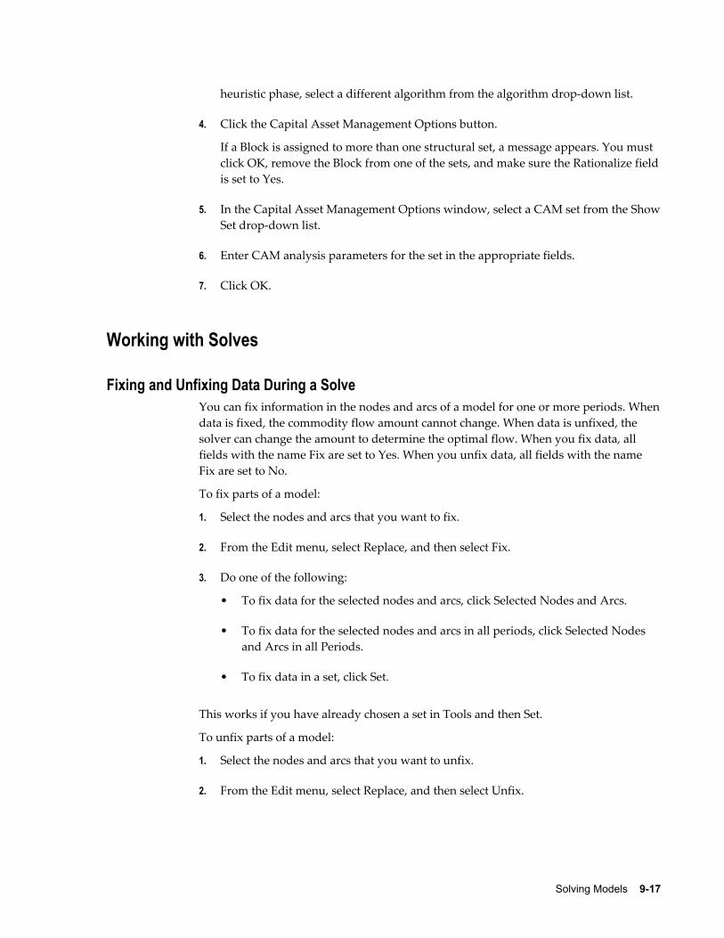
Solving Models 9-17

heuristic phase, select a different algorithm from the algorithm drop-down list.

4. Click the Capital Asset Management Options button.

If a Block is assigned to more than one structural set, a message appears. You must click OK, remove the Block from one of the sets, and make sure the Rationalize fieldis set to Yes.

5. In the Capital Asset Management Options window, select a CAM set from the ShowSet drop-down list.

6. Enter CAM analysis parameters for the set in the appropriate fields.

7. Click OK.

Working with Solves

Fixing and Unfixing Data During a SolveYou can fix information in the nodes and arcs of a model for one or more periods. Whendata is fixed, the commodity flow amount cannot change. When data is unfixed, the solver can change the amount to determine the optimal flow. When you fix data, all fields with the name Fix are set to Yes. When you unfix data, all fields with the name Fix are set to No.

To fix parts of a model:

1. Select the nodes and arcs that you want to fix.

2. From the Edit menu, select Replace, and then select Fix.


• To fix data for the selected nodes and arcs, click Selected Nodes and Arcs.

• To fix data for the selected nodes and arcs in all periods, click Selected Nodes and Arcs in all Periods.

• To fix data in a set, click Set.

This works if you have already chosen a set in Tools and then Set.

To unfix parts of a model:

1. Select the nodes and arcs that you want to unfix.

2. From the Edit menu, select Replace, and then select Unfix.



• To unfix data for all nodes and arcs select All Nodes and Arcs.

• To unfix data for the selected nodes and arcs, select Selected Nodes and Arcs.

• To unfix data for the selected nodes and arcs in all periods, select Selected Nodes and Arcs in all Periods.

• To unfix data in a set, select Set.

This works if you have already selected a set in Tools and then Sets.

Fixing or Unfixing Data in a Period

To fix or unfix data in a period:


2. In the Periods window, click the Fix/Unfix button.

3. In the Fix/Unfix Period window, from the Period field, select the periods that contain the data that you want to fix or unfix.


• To fix or unfix data for all nodes and arcs in the selected periods, click the All button in the Apply To area.

• To fix or unfix data for the selected nodes and arcs in the selected periods, click the Selected button in the Apply To area.

5. Click either the Fix button or the Unfix button.

Determining the Net Change from the Last SolveYou can set a solve baseline to compare the results of a solve with the results of subsequent solves. This process is useful for net-change reporting and "what-if" scenarios. Each node and arc has a Baseline field and Delta field.

Once set, the Baseline field holds the value of the Used, Storage, or Flow field (depending on the object type) and is not changed by subsequent solves. The Delta fieldshows the difference between the current value and the Baseline.

You can also create a net-change report, which allows you to make custom reports to compare different solves from the baseline in report queries. Report queries can also be made to compare the criteria that are interesting to you: manufacturing, storage, distribution, and so on. Percent differences and totals can be calculated in the report queries output if needed. This procedure works with the restricted solve because you can restore the baseline as your working solution at any time.

Solving Models 9-19

You can use the batch commands setbaseline and restorebaseline to set and restore the baseline.

To set the baseline, from the Solve menu, select Baseline, and then select Set. The current Used, Storage, or Flow field value is copied to the Baseline field.

To restore the baseline, from the Solve menu, select Baseline, and then select Restore. The Baseline field value is copied to the Used, Storage, or Flow field.

To create a net-change report:

1. From the Solve menu, select Baseline, and then select Set.

The current Used, Storage, or Flow field value is set as a baseline for your working solution.

2. Modify supply chain data and re-solve the model.

3. Create a report query with the following pattern for the Delta field: <>0

4. Apply the report query and view the report in the Data Editor.

Discarding the Basis Stored in the ModelCircumstances can arise in which you want to reset the basis that is stored in the model.The next solve is then a cold solve, which does not use the basis from a previous solve. This solve usually takes much longer to complete than a warm solve, which starts from an existing basis that is usually close to optimal.

Discarding the advance basis has no effect on network and barrier solves since these algorithms do not start from an existing basis. You can also reset the basis with the batch command discardbasis.

To discard the basis stored in the model:

1. From the Solve menu, select Discard Advance Basis.


Heuristic Results from Previous SolvesThe system can use the heuristics results from previous solves. The system extracts information from the current model, and if this information is still feasible for the heuristic constraints, it installs these results. If the stored information is not present or invalid for some nodes, the heuristics are run for those nodes.

To use heuristic results from a previous solve:


2. In the Solve Configuration window, select Use Old from the On/Off/Use Old


drop-down list.

Resetting Heuristic InformationYou can remove information from previous solutions from parts of a model. You can use this technique to run a local heuristics solve again if the heuristics initially failed to find a good solution in some parts of the model. This technique is also useful if some local changes probably do not affect other parts of the model. You can select to solve only parts of the model again.

To reset heuristic information:

1. Select the nodes to reset.

If you select a Block node, all of the nodes in the Block node are reset.

2. From the Edit menu, select Replace, then Reset.

3. In the Fix Status area, select Ignore, Unfix, or Fix.

4. Select the heuristics to reset in the Reset Solutions area.

5. In the Apply Periods area, select one of the following:

Option Description

Selected Objects Only resets the elements in the periods where they were selected. Selecting an element in multiple periods can be done by changing periods with the period tabs on the bottom of the main system window and holding the control key when clicking an object so that the element is added to the setof selected elements.

All Resets the selected nodes in all the periods of the model.

Range Resets selected nodes in all the periods in the specified range. No changes are made if the From period is later than the To period.

6. Click OK.

Solving Models 9-21

Determining Available System MemoryStrategic Network Optimization requires memory for a variety of functions. Memory is required for the executable; to store the model, for the solver, for buffers and pivots to solve, and to keep an extra copy resident in memory, depending on the solver algorithm.

The Barrier solve can take up to twice the amount of memory as the other solver algorithms and can be taxing on a system's memory. A useful rule of thumb is to provide five times the model size in memory (including swap space) for the model to solve. You can determine and display the total amount of memory on the system that is available to Strategic Network Optimization.

The two kinds of memory are:

• Physical: the actual hardware memory components on the system

• Swap space: the area of disk or memory reserved or configured for swapping out processes or portions of processes

If enough memory is not available, your operating system might need to be reconfigured, or more memory might have to be added to successfully run Strategic Network Optimization.

To determine available system memory for Strategic Network Optimization:

1. From the Start menu, select Programs, select Oracle Supply Chain Planning, select Strategic Network Optimization x.x.

2. At the prompt, enter:memtest

The command displays the amount in both megabytes and bytes.

Infeasible Solves

Troubleshooting Infeasible SolvesInfeasible solves can be caused by a variety of factors. If a model is infeasible, you can try the following techniques to solve the problem:

• Check for fixed values on arcs or nodes in the model. This problem is the leading cause of infeasibility.

• Check for infinite penalty costs on minimums, maximums, and safeties.

• Check for infinite backorder costs in StorageCover and StorageDemand nodes.


• Reduce the size of the model (by deleting periods or components) and solve the model again to find the infeasibility.

• Review the linx.log file in detail.

Accepting a Solution with Unscaled InfeasibilitiesBy default, the Strategic Network Optimization solver scales a problem before solving itin order to improve solve time performance. After the solver finds an optimal solution, it checks for any violations of optimality or feasibility in the original, unscaled problem. When a scaled problem is solved within the specified feasibility tolerance, but the corresponding unscaled solution contains one or more variables that violate the feasibility tolerance, a solve warning message appears.

This message indicates that an optimal solution has been found, but it contains unscaledinfeasibilities. This could be the result of a row that has cost coefficients with different magnitudes. The user can choose to accept or reject a solution that is optimal with unscaled infeasibilities. In batch mode, a solution that is optimal with unscaled infeasibilities is automatically accepted.

The problemstats Batch CommandStrategic Network Optimization accepts a solution with unscaled infeasibilities because it is likely the feasibility violation is relatively minor. It might be possible for the solver to find a better solution even though the model contains unscaled infeasibilities, or it might be necessary to revise some of the costs in the model. The problemstats batch command can be used to locate this information. The command syntax is as follows: problemstats

The following is an example of the data displayed after the problemstats batch command has been entered:Variables : 36480Linear constraints : 24840Nonzeros : 69036RHS nonzeros : 463RHS nonzeros : Min: 2 Max: 184Linear constraints nonzeros : Min: 1 Max: 100Objective nonzeros : 20161Objective nonzeros : Min: 0.0025 Max: 20000Variables : Min LB: 0 Max UB: 1950000

The Min and Max values are for right-hand side (RHS) nonzeros. Linear constraints andobjective nonzeros provide the range of these coefficients. For example, 2 and 184 are the are the smallest and largest coefficients of a sample problem. In most Strategic Network Optimization models, the objective nonzeros are the quantities which can be reviewed.

The objective function in a model has coefficients that represent real costs and penalty costs. Wide ranges between small real costs and large penalty costs often exist. If the

Solving Models 9-23

range between the Min and Max value exceeds 109, you might need to revise some of the model costs that produce these numbers. In the example above, the range of coefficients in the objective function is 20000/0.0025 = 8 x 106 which is within the recommended range.

Locating Elements that Cause InfeasibilityYou can select the Use IIS (irreducibly inconsistent set) Finder for Infeasible Set option in the Solve Configuration window.

If a Primal solve detects an infeasibility, a warning dialog is displayed and you can decide to create an Infeasible set. If this option has been selected, you can determine which algorithm is used to determine the Infeasible set.

If the option is not selected, you use the algorithm originally used by Strategic Network Optimization to determine infeasibilities.

This algorithm looks for the constraints in the problem that could not be satisfied with the Primal solver method. If the Use IIS Finder for Infeasible Set option is selected, the IIS finder is used. This algorithm detects an inconsistent set of elements that can be made feasible by making a change to one of the elements in the set, and isolates the cause of the infeasibility. This algorithm generally takes more time than the original infeasibility finding algorithm.

The finder takes the linear program and corresponding basis as input, and produces an irreducibly inconsistent set of constraints (IIS). An IIS is a set of constraints and column bounds that is infeasible, but becomes feasible if any one member of the set (any constraint or variable) is dropped. Once an IIS is produced, it can be inspected to determine the cause of the infeasibilities.

By reducing the problem to a smaller subset of constraints and bounds, pinpointing problems is typically much easier. An infeasible problem can contain many independent IISs. The finder finds only one. After correcting the infeasibility caused by a single IIS, a problem can remain infeasible, so it might be necessary to run the finder more than once.

You can find the elements that created certain variables and constraints, which is useful for debugging certain solver error messages that can be displayed by a network primal solve.

If an infeasibility is detected during a preprocessing phase, a solve message displays theconstraint or variable that caused the infeasibility. You can then detect where in your model the infeasibility occurs.

To locate elements that cause infeasibility during a preprocessing phase:


• To display the Constraint Finder, select Find from the Edit menu, and then select Constraint.


• To display the Variable Finder, select Find from the Edit menu, and then select Variable.

2. In the Finder window, enter the element number in the Find element field and click Find.

For example, if the error message displays an inequality for constraint 4 (c4), enter 4.

The information, such as node, arc, period, or commodity, appears in the other field in the window. You can use this information to locate the element that is causing the problem.

To find nodes and arcs that caused violations or an infeasible solve:

1. Solve the model. An information window appears if any solve warnings exist.

2. If an information window appears, click OK.

The Sets and Set Browser windows display sets of nodes and arcs that caused the solve warnings.

or


2. In the Sets window, display User Sets.

3. In the Sets area, select the Infeasible set, or the Over, Under, or Over or Under set inwhich the violations occur.


• To select nodes and arcs that belong to the set in the model, click Uncover.

• To view nodes and arcs that belong to the set, select Browser from the Edit menu.

• To display data for the selected Set, select a query from the Query Set menu.

Adjusting Solver Tuning Parameters

Types of Solver Tuning ParametersStrategic Network Optimization uses linear programming to solve supply chain models. There are different types of linear programs that are used to solve models, suchas Network Primal, Barrier, Dual, Network Primal, and Network Dual. While these linear programs all produce the same solution, they use different speeds and factors to perform calculations Depending on the size, complexity, and constraints of the model,

Solving Models 9-25

and the solver algorithm and the heuristics you select, one linear program could be more optimal than another.

For example, certain models converge more quickly using Network Dual rather than Barrier. If solve time is critical, you should experiment with different linear programs tosee which one produces the fastest solve. However, if time is not critical, you could baseyour choice of linear programs on a different set of criteria.

Strategic Network Optimization has a default set of solver parameter values such as Markowitz Pivot Tolerance and Scale Algorithm Indicator. It is also useful to adjust solver parameters in order to determine if a different set of solver parameter values reduces solve time or increases the stability of the solve.

The solutionquality Batch CommandThe solutionquality command displays data about the maximum reduced-cost infeasibility and the maximum bound infeasibility. The command syntax is as follows: solutionquality

The following is an example of the data displayed after the problemstats batch command has been entered: Max unscaled (scaled) bound infeas.= 0(0)Max unscaled (scaled) reducedcost infeas.= 3.08553e-12(3.08553e-12)Max unscaled (scaled) primal residual (|Ax-b|)= 4.70834e-12(3.63798e-12)Max unscaled (scaled) dual residual (|c-B'Pi|)= 2.91038e-11(2.55983e-09)Max unscaled (scaled) X value = 55288.3(55288.3)Max unscaled (scaled) slack value = 55288.3(55288.3)Max unscaled (scaled) value in dual solution (pi)= 450000(2.62419e+08)Max unscaled (scaled) reduced-cost = 483965(483965) Kappa = 6.4972e+07

The solutionquality command can identify inconsistent behavior that contributes to the improper model conditioning such as:

• Inconsistent results with different parameter settings.

• Modifications to a linear programming problem which caused inconsistent results that affect the solution, such as adding a constraint that the current solution does not violate.

• Inconsistent results with a relatively small change in data.

The solutionquality batch command allows the user to search for linear programming problems. It displays the magnitude of residuals associated with the solution such as the accuracy with which the solution satisfies constraints and bounds and the condition number of the optimal basis; kappa.

Kappa, the basis condition number, measures the sensitivity of the model data. It is equivalent to the number of places in the precision that can be ignored. The kappa valueprovides the condition number of the optimal basis. Most computers have a precision of1e-16and the error for the solution value is approximately equal to:

[(computer precision)* kappa].


The kappa value can be significant in determining the extent of damage caused by a round-off error. For example, if kappa = 1.3672e11, there are 5 accurate places left (for example, e-16* e11= e-5). Round-off errors of 1e-5can multiply the right side of the matrix or objective coefficients. Therefore, even small problems can magnify the round-off error.

If kappa is relatively low (e.g. =1e8), you can be confident about the solution. If kappa ishigh, or if reducing the tolerance does not help, then you should consider revising the model because the current model might not be able to produce a reliable result.

Turning Scaling OffIf unscaled infeasibilities occur in the primal problem, it is recommended that you turn scaling off and solve the problem using the Dual Simplex method with the previous basis solution.

To turn scaling off:


2. In the Solve Configuration window, click the Advanced button.

3. In the Solver Parameters window, change the Scale Algorithm Indicator parameter from 0 to – 1.

Optimality and Feasibility ToleranceAdjusting the optimality or the feasibility tolerance can produce a better solution. Although increasing these tolerances could produce a better solution, lowering these tolerances could produce unwanted side effects such as instability.

The maximum reduced cost infeasibility identifies a value for the optimality tolerance that causes the solver to perform additional iterations. If a solve terminates with an optimal or infeasible solution, and the maximum reduced-cost infeasibility is only slightly smaller in absolute value than the optimality tolerance, solving the problem with a smaller optimality tolerance could result in an improvement in the objective function.

To change the optimality tolerance:



3. In the Solver Parameters window, enter a value between 1e-9 and 1e-1 (=0.1) in the Reduced Cost Tolerance field.

The default is 1e-6.

The maximum bound infeasibility identifies the largest bound violation. This

Solving Models 9-27

information could help determine the cause of infeasibility in a linear programming problem. If the largest bound violation exceeds the feasibility tolerance of the problem by only a small amount, you might get a feasible solution to the problem by increasing the feasibility tolerance.

To change the feasibility tolerance



3. In the Solver Parameters window, enter a value between 1e-9 and and 0.1 in the Feasibility Tolerance field.

The default is 1e-6.

The Scale Algorithm IndicatorThe Scale Algorithm Indicator is a solver parameter that can improve model conditioning. Setting the scaling parameter helps if you have a combination of large andsmall coefficients in the constraint matrix. The Markowitz Pivot Tolerance instructs the solver to use a less tolerant pivoting scheme during the basis factorization. These parameters can reduce the round-off error on numerical problems that are not well constructed.

To set the level of scaling to aggressive:



3. In the Solver Parameters window, enter 1 in the Scale Algorithm Indicator field.

Problems in which even minor changes in data result in major changes in solutions could improve with different scaling settings. Scaling attempts to fix linear programming problems by multiplying rows or columns by constants without changing the original logic of the problem. If your linear programming problem cannot remain feasible during a solve, you should try a different scaling setting.

Available settings for the Scale Algorithm Indicator are:

Value Meaning

–1 No scaling.

0 Equilibration scaling. This is the default.


Value Meaning

1 Aggressive scaling.

Increasing the Markowitz ToleranceThe Markowitz tolerance controls the kinds of pivots permitted. Increasing the Markowitz tolerance can also provide a more optimal solution to complex linear programming.

To increase the Markowitz feasibility tolerance:



3. In the Solver Parameters window, enter the maximum value, 0.999 in the Markowitz Pivot Tolerance field.

If the Markowitz tolerance level is set near its maximum value of 0.99999, iterations could be slower, but they are more stable.

Avoiding Bounds Larger than 1e9

If you avoid variable bounds larger than 1e9, a more optimal solution could be reached. Large bounds can cause large round-off errors, and finite bounds should always be as small as possible without compromising the meaning of the associated variable and constraints. Large upper bounds could also result in excessive memory use and cause difficulties during pre-solve. For very large bounds, consider using infinity; Max = *.

Linx.log File SettingsThe first phase of a solve, pre-processing, simplifies the problem using the pre-solver and aggregator. In the second phase, the solver searches for a feasible solution. In the final phase, the solver searches for the optimal, feasible solution and writes solver log messages to the linx.log file. By default, the linx.log file is located in either the \bin directory or in the directory specified by the LINXLOGDIR environment variable. The amount of detail written to the linx.log from the solver can be specified using the Simplex Display Level parameter.

Available settings for the Simplex Display Level parameter are:

Solving Models 9-29

Value Meaning

0 No iteration messages until solution.

1 Iteration info after each refactoring (default).

2 Iteration info for each iteration.

The linx.log file contains solver iterations that include the current iteration number and either the current scaled infeasibility during the second phase or the objective function value during the final phase. Once the optimal solution has been found, the objective function value and solution time are displayed. The information in the linx.log file is useful for monitoring the rate of solver progress.

If a problem repeatedly becomes infeasible in the final phase of a solve, it could be caused by numerical difficulties. Slow progress during the second phase is often causedby similar numerical difficulties that are less obvious because feasibility is not determined as in the final phase. In both cases, increasing the Markowitz Pivot Tolerance to 0.99999 could help.

The Feasibility Tolerance specifies the degree to which a problem's basic variables couldviolate their bounds. Feasibility influences the selection of an optimal basis and can be set to a higher value when a problem is having difficulty maintaining feasibility during the final phase . If you find reports of infeasibility during optimization in the linx.log file, a small increase in the feasibility tolerance could improve performance. You could also decrease the tolerance level if there is any doubt that a solution is optimal. If the feasibility tolerance is set too low, the solver could mistakenly conclude that a problem is infeasible.

Finding or Replacing Data 10-1

10Finding or Replacing Data


• Find and Replace Overview

• Performing a Find

• Performing a Replace

Find and Replace OverviewIf you want to determine which nodes or arcs in a model have certain characteristics and data values, you can perform a find on the nodes and arcs that meet specific criteria. Nodes that are found can also be selected. The system can highlight selected nodes to enable you to see which nodes or arcs have the specified characteristics. For example, you can perform a find on all machine nodes with 100 percent utilization and these nodes can then be selected.

You set up searches by using combinations of numeric or character values, expressions, and wildcard characters. When the system completes a search, it displays a message that indicates the number of results found. A User set that is named -Found is also created. You can locate nodes or arcs in an entire model. You can select nodes or arcs in a model and determine which of the selected nodes or arcs have particular characteristics. You can select nodes or arcs in one time period of a model and determine which of the selected nodes or arcs meet specified criteria in all time periods of the model. You can also restrict a search to nodes or arcs in a set.

Your ability to find numeric values correctly is partly determined by the number of decimal places displayed in properties windows. For example, if the Display Precision is set to zero, you do not see decimal points in the Properties window; the system truncates the values. With Display Precision equal to zero, a Storage value of 1300.7 appears as 1300 in the Properties window. However, if you set up a search and indicate that Storage equals 1300, the system does not select the node.

You can also use comparison symbols, such as =, <, >, AND, OR, and XOR. In addition, in Find windows, you can begin an expression with a comparison symbol. The


left-hand side is the implied field name.

Examples

Assume that you have spherical tanks modeled as Storage nodes and you want to find the nodes in which the value in the maximum volume field is greater than or equal to your 10-m radius tanks. To find the nodes, you would enter the following expression in the Max field of a Storage Find window:x>=4/3*PI()*POWER(10,3)

This formula finds a Storage node only when the value in the Max field is greater than or equal to the calculated value of the following equation: UNRECOGNIZED STYLE ->class=CBLinkScreen>[INT: 483331]

In the next example, assume that you want to find demand data points that are outside of the average demand values. You could use the following expression in the Demand field of a StorageDemand Find window: x <= AVEPERIODS(#Demand)*.8 OR x >= AVEPERIODS(#Demand)*1.2

This expression finds results only when the value in the Demand field is 20 percent above or 20 percent below the average value for demand across all periods.

Exporting Results from a FindYou can also find nodes and arcs in a model that have certain qualities and export the data to a file. For example, you can find all Machine nodes with a utilization of 100 percent and then export their names to a file.

When a find is completed, a message window displays the total number of nodes and arcs found, and they are then selected. The system also creates a User set named -Found. The data is exported to the file specified in the File name field.

The Export tab in the Find and Export window allows you to specify which fields are exported, as shown here below:

You can find and export all nodes or arcs in a model, selected nodes or arcs, or nodes or arcs in a set.

Find and Replace Pattern OverridesYou can use overrides in any unused field of the Find and Replace window. The syntax is as follows:

override=expression

The possible values for override are:

• commoditydescription

• commodityfamily


• location

• blockname:n

where n is the block level.

The expression can be any regular find expression, and can include wildcard characters.

Example: Using Find Pattern Overrides

The following table displays examples for using find pattern overrides:

Override Finds

commodityfamily=Fam1|Fam2|Fam3 Arcs that carry a commodity with the family name Fam1, Fam2, or Fam3

location=Factory 1 Nodes of a certain kind in the block Factory 1

commoditydescription=*Export* Arcs that carry a commodity with a description that contains the word Export

blockname:1=Group 2 Nodes of a certain kind with an immediate parent block has the name Group 2

Expressions and FunctionsYou can use expressions and functions in Find windows to locate data. An expression can be made up of the following components:

Component Example Explanation

Number 400 Any number.

Variable x Represents the field name. Optional in Find windows and report queries.


Component Example Explanation

Field name Demand The field name is the name of a field in a Find, Replace, or Report Properties window. If the field name contains spaces, enclose it in double quotation marks.

Some functions require a # before the field name.

Symbol + - * / () Addition, subtraction, multiplication, division; use round brackets to specify order of operations.

Function ABS(Demand) The functions you can use are largely the same as those available in the Data Editor.

You can use the comparison symbols in the following table.exp1and exp2 represent expressions.

Expression Meaning

exp1 = exp2 Returns true if the expressions are equal. Otherwise, returns false.

exp1 != exp2

exp1 <>

Returns true if the expressions are not equal. Otherwise, returns false

exp1 < exp2 Returns true if exp1 is less than exp2. Otherwise, returns false.

exp1 > exp2 Returns true if exp1 is greater than exp 2. Otherwise, returns false.

exp1 <= exp2 Returns true if exp1 is less than or equal to exp2. Otherwise, returns false.

exp1 <= exp2 Returns true if exp1 is greater than or equal to exp 2. Otherwise, returns false.


Expression Meaning

exp1 AND exp2 Returns true if both expressions are non-zero or true. Otherwise, returns false.

exp1 OR exp2 Returns true if one or both expressions are non-zero or true. Otherwise, returns false.

exp1 XOR exp2 Returns true if exactly one expression is non-zero or true. Otherwise, returns false.

You can start an expression with a comparison symbol. The left side is the implied field name.

The following general syntax rules must be followed in all functions and expressions:

• Every function must be followed by a left and right parenthesis. For some functions the parentheses remain empty-for example, TRUE() and PI(). For other functions, the parentheses must contain arguments-for example, SUM(Prd1,Prd2).

• Variables in functions are indicated by x, y, or some other variable name. In place ofthe variable name, you can enter:

• A number

• A field name, if the field contains a number

• A function or expression that results in a number

• Variable lists in functions are indicated by a,b…. In place of this, you can enter:

• A list of numbers

• A field name, if the field contains numbers

• A list of names of fields that contain numbers

• A list of functions or expressions that result in numbers

• You can use multiple functions and nested functions in an expression.

• Do not mismatch data types. For example, a string function can use only string values, and a date function cannot use integers. Whether you use logical statements,numeric calculations, or date arithmetic, use only one data type in an expression.

The following are examples of valid expressions:


Demand*100IF(x>10000,x/10,x)COS(Value)

Performing a Find

Performing a Find on Selected Nodes or ArcsYou can perform a find on all nodes and arcs in a model or on selected nodes or arcs in a model. The find can be performed on the current period or on all the periods in the model.

To perform a find:


• Select the nodes and arcs on which you want to perform the find. From the Editmenu, select Find, then Nodes or Arcs.

• Right-click a node or arc and select Find. The Find and Replace window appears.

2. In the Scope area, for Period(s) select either All or Current. For Search, choose Selected.

3. Enter the expressions or data that you want to find in the appropriate fields.

4. Optionally, you can click the Add To Favorites button to save the find criteria as a favorite in the Model Workspace.

5. Click the Find button.

The Results tab lists the found nodes or arcs.

To perform a find on all nodes or arcs in a model:

1. From the Edit menu, select Find, then Nodes or Arcs.

2. In the Scope area of the Find and Replace window, for Period(s) select either All or Current.

3. For Search, choose Model.

4. In the Find In drop-down list, select Arc to perform the find on all arcs in the model. Select Node (all types) to perform the find on all nodes in the model.

5. Enter the expression or data that you want to find in the appropriate fields.

6. Optionally, you can click the Add To Favorites button to save the find criteria as a


favorite in the Model Workspace

7. Click the Find button.

The Results tab lists the found nodes or arcs.

Find ResultsWhen a Find is performed, the Results tab is automatically displayed in the Find and Replace window. The Results tab displays a list of all found nodes or arcs

To launch properties windows from the Results tab:

1. Select a node or arc from the list.


3. Click the View button.

Click the Show button to unblock and display all found nodes or arcs in the model workspace.

Performing a Replace

Replace ResultsAfter a find is performed, you can perform a replace in the found nodes or arcs. The scope of the replace is the same as the scope of the find. For example, if the find was performed on only the current period but for the entire model, the replace is only performed on the current period but for the entire model.

To perform a find and replace for selected nodes and arcs:

1. From the Edit menu, select Find, then Nodes or Arcs.

2. In the Find and Replace window, click the Replace tab.

3. In the appropriate fields, enter the expressions or data that you want to replace.


When a replace is performed, the Replace Results window appears. In the Replace Results window, the From column displays data before the replace, and the To column displays the data after the replace. You can launch properties windows and undo a replace in the Replace Results window.

To launch properties windows from the Replace Results window:

1. Select a node or arc from the list.



3. Click the View button.

To undo the changes made in a replace, click the Undo All button.

To export the results of a find:

1. In the Export tab of the Find and Replace window, select the fields to export.

2. Click the Export button.

3. In the Export As window, specify a name and location for the export file and click the Save button.

Reporting and Extracting Data 11-1

11Reporting and Extracting Data


• Reporting and Extracting Data Overview

• Extracting Data Using Report Queries

• Organizing Report Queries Using Groups

• Report Overrides

• Extracting Data Using Commands

• Working with Publishing Profiles

Reporting and Extracting Data Overview

Reports and Report QueriesReport queries are patterns of nodes and arcs used for extracting data from a model. This extracted data can be viewed in the Data Editor, used to create reports or edit data, and exported to other systems. To build a report, you:

1. Decide what information you want to extract from the model.

2. Determine where the data resides (which type of nodes and in which arcs).

3. Make a report query which will extract this information.

Report queries look like small models. However, the nodes and arcs in a report query do not represent model data. They represent nodes and arcs in a model from which youwant to extract data. Before building the report query, you must first decide what information you want to extract from the model. You then determine which nodes and arcs contain this information.

Your report query must include nodes and arcs of the type that you want to extract datafrom. For example, if you conclude that the information you want to extract resides in


arcs which flow from Storage nodes into Demand nodes, your report query must contain one Storage node, with an arc attached to it, flowing into one Demand node. Next, you create and set up a report query which will extract the information.

To make a report query, you:

• Create nodes, arcs, and commodities that represent the nodes, arcs, and commodities in the model from which you want to extract data.

• Create queries which specify the information you want to extract and the layout of the extracted information.

To create the report query in the Report area of the main user interface, you create and connect nodes and arcs using the same techniques you use to build models. Next, you create report queries which specify the information that you want to extract from the model.

For example, you could request the storage and demand amounts from StorageDemandnodes in your model. After opening or building a report query, you extract the data by running the report.

When you run a report, Strategic Network Optimization:

• Finds nodes and arcs in the model that match the report query pattern

• Extracts data specified in the report query from nodes and arcs that match the report query patterns

• Saves the data to the .smart file

• Launches the report in the Data Editor window

An Example of Building a ReportWhen building a report query, you need to know what you want to show in your report. In this example, suppose you want to produce a report which displays the flow of all the coffee brands from all of the distribution centers to all of the customers. You could get this information by going into the model and manually performing individualarc queries. However, you would have to do many individual arc queries in each period. This could be very time consuming, not visually appealing, and prone to humanerror, especially in large models.


Now that you have decided what information you want to see in your report, you need to figure out where that information is located in your model. You determine that the information you want to extract resides in arcs which flow from StorageDemand nodes into Demand nodes. Next, you construct a report query which will extract data from all the arcs that flow from StorageDemand nodes into Demand Nodes.

• In the Model Workspace area, click Reports and then select New Report. A blank Reports workspace is displayed in the main user interface. To return to your model,click Model Data in the Model Workspace area.

• In the Reports area of the main user interface, create a StorageDemand node with an arc connecting it to a Demand node, and a commodity carried in the arc. You canname the nodes, arc, and commodity anything you want. If you provide a label, the information is included in the report. In the example below, you can see the DC1–Mellow StorageDemand node, with an arc connecting it to the Vancouver Demand node. This is what a report query looks like.

• Strategic Network Optimization will to go into the model and find all the instances of this combination of nodes and arcs. But first, you need to use report queries to define the data fields that you want to extract from the model and place include in your report.

In this example, the following report queries are defined:


• The data in the above example is well defined, in that the source (DC), commodity (Commodity), the amount of flow (Flow), and the period (Month) are all identified with a meaningful label. This is the data that is displayed in the report.

• Although a Period field appears in each properties window, you only need to define it once.

• The label DC=location is a report query override. This populates the DC column in the report with all the values in the location field.

When you run this report, the Data Editor appears, as seen here below:


Strategic Network Optimization extracts the requested information and puts it in a tableformat in the Data Editor. From here, you can save or export this report. When using the Data Editor, you can copy and paste data from one cell to another. You can copy from and paste to multiple cells by using Shift + arrow keys or Shift + left-click at the end of a range of cells. You can use Ctrl C , Ctrl V, or select copy and paste from right-click menus.

Extracting Data Using Report Queries

Opening Report QueriesWhen working with report queries in the Reports main user interface, a blank workspace is displayed and you can't see your model. To return to your model, click Model Data in the Model Workspace area.

To select a report query in the Model Workspace area, left-click on it once. If you double-click on the name, the report query runs and the Data Editor launches, displaying the report.

To open a report query, in the Reports area of the Model Workspace:

1. Right-click on Reports and select Add Report.

2. In the Open window, browse to the directory where the report query resides. All report queries have .smt extensions.


3. Select a report query and click Open.

Running Report QueriesTo run a report query, in the Reports area of the Model Workspace, double-click the report query. The Data Editor launches and displays the report which contains data extracted from the report query. You can also:

1. Right-click on a report query.

2. Select Open and then select On Model.

To run report queries for a selected part of a model:

1. Select the part of a model that you want to query.

2. In the Reports area of the Model Workspace, right-click on a report query.

3. Select Open and then select Selected Nodes and Arcs.

To run report queries for a set:

1. Select a set from the Sets area of the model.

2. In the Reports area of the Model Workspace, right-click on a report query.

3. Select Open and then select Sets.

When you open reports from the Reports level of the Model Workspace by right-clicking on Reports, selecting Open, and then one of Open options, the action applies to all report queries listed in the Reports area. For example, if you right-click on Reports, select Open, and then select Selected Nodes and Arcs, every report query in the list will be run for selected nodes and arcs.

Marking and Unmarking for AutoOpenReport Queries can be marked or unmarked for AutoOpen. By default, when you open a report query or build a new one, it is marked for AutoOpen. All report queries which are marked for AutoOpen can be run at once from the Reports level above them. When a report query is marked for AutoOpen, a blue checkmark appears next to it as seen here below. The first and third report queries are marked for AutoOpen and the second and fourth are not.


To mark a report query for AutoOpen:

1. Right-Click the report query.

2. Select Mark for AutoOpen.

To unmark a report query for AutoOpen:

1. Right-Click the report query.

2. Select Unmark for AutoOpen

To mark all report queries for AutoOpen:

1. Right-click on Reports.

2. Select Mark All for AutoOpen.

To unmark all report queries for AutoOpen:


2. Select Unmark All for AutoOpen.

To run all report queries which have been marked for AutoOpen:


2. Select Open Marked and then select one of the following:

• On Model


• Sets Building Report Queries

Building Report QueriesTo build a report query, in the Reports area of the Model Workspace:

1. Right-click Reports.


2. Select New Report.

3. In the Reports workspace, create nodes, arcs, and commodities that represent the nodes, arcs, and commodities in the model from which you want to extract data.

4. In the Reports area of the Model Workspace, right-click the report query and select Save.

Note: When you save a report query, it is saved as a separate file with a.smt extension. If you rename this report query in the user interface, it renames the actual file. However, deleting the file in the user interface does not actually delete a file.

To set up a report query:

1. In a report query, right-click a node or arc from which you want to extract data.

2. Select Node Properties or Arc Properties.

3. In the Report Properties window, enter a heading for each field from which you want to extract data in the Label column.

Data is extracted only from fields that have a heading in the Label column. Extracted data appears in the Data Editor under the headings that you enter.

You can also enter report overrides in the Label column. Report overrides enable you to extract information about items that you cannot find directly in a report query. For example, you can use report overrides to find the total amount of commodities flowing into or out of a node.

4. If you want to extract data only from nodes or arcs that meet certain criteria, enter search expressions in the Pattern column.

You can use any search expression that you can use for Find functions.

5. Click OK.

Deleting a Report QueryTo delete a report query, in the Reports area of the Model Workspace:

1. Right-click a report query.

2. Select Delete.

The system prompts you to confirm whether you want to remove the selected report query.

3. Click OK.


The report query is removed from the Reports area of the Model Workspace. However, it is not actually deleted from the folder where it resides, and you can reload it to your model at any time.

Exporting Report Query ResultsYou can export the results of a report query to either a XML file or a comma-separated variable file (CSV). These formats are useful for importing the data into Windows applications, particularly for database tables and reporting purposes.

To export report query results:

1. Right-click the report query that you want to export.

2. Select Export.

3. In the File name field in the Export As window, enter a name for the file.

4. In the Save as type drop-down list, select either XML or CSV.

5. Click Save.

The report is saved with the model.

Specifying the Default Location of Report QueriesYou can change the default location where new reports are saved.

To specify the location:


2. In the View Options window, click the Report tab.

3. Click the Browse button.

4. In the Browse for Folder window, specify the default directory.

If you move the location of a report query and the system can't find it, a red X is put through it's name in the Reports area of the Model Workspace. To fix this:


2. In the View Options window, click the Report tab.

3. Click the Repair invalid reports button.


Organizing Report Queries Using Groups

Creating a Report Query GroupTypically, you create more than one report query for a model. To organize your report queries, you can create a list of them in the Model Workspace. This list is called a report query group. You can open a report query group and immediately have access to all related report queries. You can run all the report queries in the group at once, or only certain report queries within a group.

The name of each report query in a group is listed beneath the name of the group. You can easily switch from one report query in the group to another by left-clicking once thename of the report query once. If you double-click on the report query, it runs and the Data Editor launches.

When you save a model, report query groups are saved with the file. Unlike individual report queries, they are not saved as separate files.

To create a new report query group, in the Model Workspace:


2. Select New Group.

3. Enter a name for the report query group.

4. Save the model by selecting File, then Save.

Working With Report Query GroupsTo add a report query to a report query group:

1. Right-click on a report query group and select Add Report.

2. In the Open window, browse to the directory where the report query resides.

All report queries have .smt extensions.

3. Select a report query and click Open.

To remove a report query from a report query group:

1. Right-click a report query in the report query group.

2. Select Delete.

The system prompts you to confirm whether you want to remove the selected report query.


3. Click OK.

The report query is removed from the report query group but it is not deleted from your system.

To run all report queries in a report query group:

1. Right-click on the report query group.

2. Select Open and then select one of the following:

• On Model


• Sets

To run all report queries in a report query group which have been marked for AutoOpen:

1. Right-click on the report query group.

2. Select Open Marked and then select one of the following:

• On Model


• Sets

To create a report query in a report query group:


2. Select New Report.

3. Build the report query.

Report Overrides

Using Report Overrides to Extract DataIn report queries, some of the information must be extracted using report overrides. Report overrides enable you to extract data that you cannot query directly, such as block node or commodity flow information. They allow you to specify the data and data fields that you want to extract from the report query. Report overrides can be used to extract data from or about:


• Block Nodes

• Blender Nodes

• Capital Asset Management

• Commodities and Commodity Flow

• Separator Nodes

• User-Defined Fields

Report overrides are case-independent. You can use a mixture of uppercase and lowercase letters in the overrides to make them more readable. For example, the following are all valid overrides: LocationX, outFlow, and quantityTo.

Report overrides can be entered in the Label column in a Report Properties window. The syntax is:

label=override

where:

• label is any text that uniquely identifies the data

• override is any report override

If rows with data field names in the Tag column are full, in a blank row at the bottom ofthe Report Properties window, enter a report override in the Tag column. The syntax for a report override in the Tag column of a blank row is:ov(override)

where override is any report override. In the same row, enter a label for the data in the Label column.

Report Overrides ExampleThe following example demonstrates how to do use report overrides to extract sourcinginformation from your model. Suppose you have three plants (P1, P2, and P3) represented by three block nodes, and three distribution centers (DC1, DC2, and DC3) represented by three block nodes.

All three plants ship to all three distribution centers, and you want to find the followinginformation:

Parent Block Levels in Report OverridesIn some report overrides, you must specify the level of the parent block in which you are interested in. For example, specifying the override Name=blockname:2 extracts the name of the block two levels higher than the current node. If no such block exists, the


name of the highest block is used.

Nested blocks are numbered from the innermost to the outermost level. For example, in the diagram below, each rectangle represents a block. Individual plants and distributioncenters are level 1 blocks, plants and distribution centers are level 2 blocks, and facilitiesin South is a level 3 block. To determine the longitude of the facilities in South block, you could run a report query for a node in the Plant A block, and enter longitude:3 in the Label field.

For example, consider the following Properties window. The Tag ov (blockname:1) is specified in one of the blank rows. When the report query is applied, the resulting Data Editor shows both the name of the node (with the label NAME) and the block node to which the node belongs (with the label BLOCK).

Node Report OverridesThe following table describes report overrides:


type Returns the kind of the node. This override can be particularly useful if you use it with theIgnoreNodeType option to match on any kind of node.

x Returns or imports the x position of a node

y Returns or imports the y position of a node.

element:n Returns the nth element of the corresponding field, where n is a positive integer.


Block Node Report OverridesThe following table displays Block node report overrides:


location Returns the name of the highest block to which a node belongs.

locationfrom This override is applied to an arc and returns the name of the highest block node from which a commodity flows.

locationto This override is applied to an arc and returns the name of the highest block node into whicha commodity flows.

blockname:n Returns the name of the parent block n levels higher than the current node, where n is a positive integer.

locationx Returns or imports the x position of the highest block a node is in.

locationy Returns or imports the y position of the highest block a node is in.

longitude:n Returns the longitude of the parent block n levels higher than the current node.

latitude:n Returns the latitude of the parent block n levels higher than the current node.

mapsymbol:n Returns the symbol representing the parent block n levels higher than the current node.

Blender Node Report OverridesThe following table describes report overrides for Blender nodes:



minPartsTo Returns the minimum parts from a Blender node.

maxPartsTo Returns the maximum parts from a Blender node.

actualPartsTo Returns the actual parts from a Blender node.

violationTo Returns the parts violation from a Blender node.

underCostTo Returns the value of the underCost field in an arc that carries a commodity to a Blender node.

overCostTo Returns the value of the overCost field in an arc that carries a commodity to a Blender node.

actualFlowTo Returns the value of the actualFlow field in anarc that carries a commodity to a Blender node.

Commodity and Commodity Flow Report OverridesThe following table describes the report overrides for commodity and commodity flow:


commoditydescription For a node, this override returns the commodity description of the first attach pointon the node. For an arc, this override returns the commodity description on the arc.

commodityfamily This override returns the family field.



inflow This override returns the sum of the flow of allarcs for a commodity flow coming into a node.

The ReservedTime commodity is not includedin report = inflow override calculations. For example, this commodity is carried on the arc that leads from a Machine node to a Monitor node.

inflowto For an arc, this override returns the total flow entering the same attach point into which the arc enters.

This override is particularly useful if several arcs enter a Controller node and you want to know the total inflow of a particular commodity so that you can make a distribution-percentage sourcing matrix.

outflow This override returns the sum of the flow of allthe arcs for a commodity flow that is exiting a node.

The StorageLevel commodity is not included in report = outflow override calculations. For example, this commodity is carried on the arc that leads from a StorageDemand node to a Monitor node.

outflowfrom For an arc, this override returns the total flow leaving the same attach point from which the arc leaves.

This override is particularly useful if several arcs leave a Controller node and you want to know the total outflow of a particular commodity so that you can make a distribution-percentage sourcing matrix.

quantityfrom For an arc, this override returns the output rate from a Process node from which a commodity flows.

quantityto For an arc, this override returns the input rate from the Process node into which a commodity flows.


Separator Node Report OverridesThe following table describes report overrides for Separator nodes:

Report Override

minPartsFrom Returns the minimum parts from a Separator node.

maxPartsFrom Returns the maximum parts from a Separator node.

actualPartsFrom Returns the actual parts from a Separator node.

violationFrom Returns the parts violation from a Separator node.

actualFlowFrom Returns the value of the actualFlow field in anarc that carries a commodity out of a Separator node.

User-Defined Fields Report OverridesThe following table describes report overrides for user-defined fields:


category:n Returns the value of the Category field in a Block node.

field1:n Returns the value of Field 1 in a Block node n levels higher.





Report PatternsYou can use Pattern fields in Report Properties windows for data filtering. The following table shows examples of report patterns:

Report Overrides Matches

commodityfamily=Fam1|Fam2|Fam3 Arcs that carry a commodity with the family name Fam1, Fam2, or Fam3

location=Factory 1 Nodes of a certain kind in the block

Factory 1 location=Toronto|Chicago Returns results where the highest level Block node name is Toronto or Chicago.

commoditydescription=*Export* Arcs that carry a commodity with a description that contains the word Export

blockname:1Group 2 Nodes of a certain kind with an immediate parent block has the name Group 2

Report Queries in Specific Time PeriodsYou can query data in a specific time period by following a special syntax in the Pattern column for the Period field to specify the number of the time period, where the first time period is number.

Example: Report Queries for Specific Time Periods

To extract the first three periods, you can use either of the following methods:'Period:#1'|'Period:#2'|'Period:#3'

'Period:#1,#2,#3'

This example matches the third period to the end of the horizon:'Period:#3..*'

This example matches periods 1, 5, and 8, and relative period 3:'Period:#1,3,#5,#8'

This example matches periods 1 to 3:'Period:#1..3'

This example matches relative periods 4 and 5, absolute periods 1 to 3, and relative periods 7 to 9:'Period:4,5,#1..3,7..9'


Extracting Data Using Commands

The lxextr CommandYou can extract data from models by using report queries, but you can also use commands, such as lxextr. Extracted data is stored in an ASCII file which you can send the file to other systems for integration or reporting purposes. The lxextr command is not a batch command; it is a separate executable. You can run the lxextr command from a command line or from within a script.

When you run the lxextr command, it searches each line of a symbolic model file. The fields for lines that meet your criteria are displayed online or written to a file. Using the lxextr command is an alternative to using report queries, however, the lxextr command is less powerful than report queries. While it allows you to extract information from individual nodes and arcs, it does not enable you to examine and compare data relationships between model components.

To extract data, use the following command:lxextr -table"prefix"-matchtag="value"...-printtag ...-separatorcharacter<inputfile>outputfile

Enter the command on one line. It is shown on several lines here for clarity.

When you import a file in Oracle Strategic Network Optimization, the import file must begin with the word $begintable and end with the word $endtable. When you use the -table parameter with the lxextr command, these words are added automatically to the import file that you create.

The following table describes the parameters:


-match Defines the matching criteria. It specifies conditions that must be met for a particular line of data to be matched. Data is selected for extraction only where the specified tag has thespecified value. You can specify any number of tag=valuepairs. You must include the quotation marks around the value. The tag to use for command names is command.



-print Specifies the data fields that are extracted and printed (to the monitor or to a file). If your model has multiple periods, you should include the period tag. This parameter also supports tag-less references. If the command is tagless, @1 refers to the first value after the -print command.

The following import commands support tag-less references; addtoview, blockset, addnodetoset, addcommoditygroup, addcommoditytogroup, addperiodgroup, addperiodtogroup, addperiodgrouplevel, and usermessage.

-separator Specifies the character that separates fields in the output file. The default separator is a space. If you want to use a tab, enter the word tab for the character.

inputfile Symbolic file from which you are extracting data.

outputfile Specifies where you want the results to be sent: to the screen or to a file. If you want the results to print to a file, specify the name of the file. If you want the results to be displayedon the screen, do not specify a file.

Matching with Wildcard CharactersYou can use wildcard characters to match patterns with the -match parameter of the lxextr command. Wildcard characters for the -match parameter are the same as other wildcard characters, except for the characters listed in the following table:

Character Meaning

. Matches any single character

* Matches all characters


Character Meaning

^ The beginning of a word

$ The ending of a word

The following examples show how you can specify match patterns for the -match parameter. The examples use the following nodes:

• AppleDemand

• AppleDemand.2

• BlueberryDemand

• PlainDemand

• WholeWheatDemand

To match on any name that contains the capital letter P, enter the following command: lxextr -match name=P -print name

This command matches on PlainDemand.

To match on any name that begins with the letter a and ends with the letter d, enter the following command: lxextr -match name=^a.*d$ -print

This command matches on AppleDemand.

To match on any name that has the letter p as the second character, enter the following: name lxextr -match name=^.p -print name

This command matches on AppleDemand and AppleDemand.2.

To match on any name that starts with the letter B or P and ends with Demand, enter the following command: lxextr -match name=^[BP].*Demand$ -print name

This command matches on BlueberryDemand and PlainDemand.

To match on any name that starts with a letter from B to W and ends with Demand, enter the following: lxextr -match name=^[B-W].*Demand$ -print name

This command matches on BlueberryDemand and WholeWheat Demand.

To match on any name that begins with AppleDemand followed by the characters .2, enter the following: lxextr -match name=^AppleDemand\.2$ -print name


This command matches on AppleDemand.2.

Example: Extracting Data Using the lxextr Command

The following examples show how you can use the lxextr command. In this example, in a file called Pancakes.sym, you want to find the lines in which the symbolic tag <type>isset to Demand, and you want the values for the <name>, <min>, and <max> tags to be printed to a file called Pancakes.out. Use the following command:lxextr -table "Symbolic tag=Demand"-match type=Demand -print name min max <Pancakes.sym> Pancakes.out

The resulting file Pancakes.out contains the following lines: AppleDemand 130 130 PlainDemand 125 125 BlueberryDemand 125 125 WholeWheatDemand 125 125

Now you want to search the Pancakes.sym file and match the arcs that leave the nodes with a name beginning with Pack and enter the nodes whose name ends with Demand. You want to print the values for the <from>, <to>, and <flow> data fields to the Pancakes.out file and separate the values with tabs. You could use the following command:lxextr -table "Pack to Demand"-match from=Pack.*to=.*Demand -print from to flow -separator tab <Pancakes.sym>Pancakes.out

The resulting Pancakes.out file contains the following lines:PackApple AppleDemand 130 PackPlain PlainDemand125 PackBlueberry BlueberryDemand 125 PackWholeWheatWholeWheatDemand 125

Now you want to search the Pancakes.sym file and match on all lines that have the import command addcommodity. You want the values in the <name> field to be printed to the Pancakes.out file. This procedure creates a list of all the commodities in the model. Use the following command:lxextr -match command=addcommodity -printname <Pancakes.sym> Pancakes.out

The resulting Pancakes.out file contains the following data:"Apple""Apple Pancakes""PackagingTime""Blueberry""BlueberryPancakes""Plain""PlainPancakes""WholeWheat""WholeWheatPancakes"

The following example demonstrates tag-less -print references:lxextr -match command=usermessage -print@1 <Pancakes.sym> Pancakes.out

The resulting Pancakes.out file contains the model description for Pancakes.sym.


The lxsmartstrip CommandYou can use the lxsmartstrip command to extract data from a .smart file and convert it into a data file that can be used in a database or spreadsheet. The command removes the system-specific information from the .smart file but preserves the raw data.

The syntax is:lxsmartstrip <smartfile>strippedfile-quote-separatorcharacter

The smart file is a .smart file created by applying report queries to a model. The stripped file is the output file containing data but no system-specific information. Optionally, specify -quote if you want the output data to be enclosed in quotation marks. Optionally, specify a delimiter character with the -separator parameter. The character can be tab or semicolon.

Creating an Import File Using lxextrTo create an import file using the lxextr command, run the following command from a batch script:lxextr -table "prefix"-match tag= "value"...-print "tag" ...-separatorcharacter<inputfile>outputfile

Enclose the prefix in quotation marks. The prefix is the import prefix, which consists of the import file command and the data. When you import a file in Oracle Strategic Network Optimization, the import file must begin with the word $begintable and end with the word $endtable. When you use the -table parameter with the lxextr command, these words are added automatically to the import file that you create.

Example: Creating an Import File Using the lxextr CommandFor example, if you want to match all Supply nodes in file.sym and print the values of the <name> and <min> fields to the file file.imp, you can use the following command: lxextr -table "addnode type Supply"-match type= "Supply" -print name min-separator tab <file.sym> file.imp

This resulting file.imp file contains the following lines:$begintable 'addnode type Supply' <name> <min>"supplynode1" 0.0"supplynode2" 50.0...$endtable


Working with Publishing Profiles

Creating a Publishing ProfileIn Oracle Strategic Network Optimization, you can create user-defined menu options that run scripts which publish different sets of data and plans. You can also create and run publishing profiles that allow you to publish optimized plans. Publish actions contained in a publishing profile can be used to commit a plan during any session.

Existing report queries and script files are used as input, and the output from the publish action is data that is written to a file. Profiles determine which data to publish and allow you to initiate an integration process with an external system. You can refine your publishing preferences by editing an existing profile, or by creating a new profile for a specific business need.

Note: The publish process is not intended to generate reports.

To create a publishing profile:

1. From the File menu, select Publish, then click New.

2. Complete the following fields in the New Profile window:

Field Description

Profile name Specify a unique name for the publishing profile.

Description Optionally, specify a description for the publishing profile.

Format Select the format that will be used for publishing the data. There are three different formats: .xml, .csv, and .smart.

Output file Specify the directory in which to save the published data. You can explicitly specify the location of the directory or click Browse to browse for a directory.

3. Optionally, specify a script that will be initiated after the data is published. You can explicitly specify the location of the script or click Browse to browse for a script.

The following table lists the Batch Mode commands that can be used in a script file.


Command Description

#comment Comment line.

!command Runs the specified shell command. For example, on UNIX, ! ls displays a directory listing.

4. Select the Data Selection Tab.

5. In the Report field, specify the name of the report which will be used to publish the profile.

You can explicitly specify the location of the report or click Browse to browse for a report.

6. Click OK.

Publishing DataTo publish data using a profile:

1. From the File menu, select Publish.

2. In the Publish window, select a profile in the Profiles list.

3. Click Publish.

Editing a Publishing ProfileTo edit a publishing profile:


2. In the Publish window, edit the fields in the General and Data Selection tabs as applicable.

3. Click OK.

Deleting a Publishing ProfileTo delete a publishing profile:



2. In the Publish window, select a profile in the Profiles list.

3. Click Delete.

4. Click Yes to confirm that you want to delete the profile.

Using the Data Editor 12-1

12Using the Data Editor


• Data Editor Overview

• Configuring Data Editor Views

• Saving, Loading and Deleting Views in the Data Editor

• Changing All Values in Rows, Columns or Views

• Exporting Data from the Data Editor

• Performing Calculations on Data

• Highlighting Data

• Arithmetic Symbols and Functions

Data Editor Overview

Viewing and Exporting DataThe Data Editor displays data extracted from models by report queries and is useful for reporting Strategic Network Optimization information. As shown in the example below, the data appears in a spreadsheet format. You can view, edit, and customize the display of the data. The headings in the Data Editor are obtained from Label entries in the Report Properties windows. An example of the Data Editor can be seen here below:


The TMPDIR Environment VariableWhen you apply a report query, the system creates a temporary file that links Strategic Network Optimization and the Data Editor that contains the smart information. This temporary file is not linx.smart, and is only created when the Data Editor is launched. The default location for this temporary file is as follows:

• on UNIX: /var/tmp

• on Windows: C:\

You can change the location of this temporary file by setting the TMPDIR environment variable. The TMPDIR environment variable can also be added to a batch script.

Note: The system automatically deletes the file after the Data Editor opens.

Configuring Data Editor Views

Configuring the Data Editor LayoutTo open the Configure Layout window, from the Configure menu, select Layout.


By configuring views, you can change the appearance of the Data Editor in several waysto display your data in the most meaningful way. After you change the Data Editor's appearance, you can save your changes as a view.

To reorder columns in the Data Editor, in the Reordering columns area of the ConfigureLayout window, drag and drop the column buttons into the desired order. The columnsin the main Data Editor window are reordered.

To spread a column horizontally in the Data Editor, drag a column button from the Reordering columns area, and drop it into the Spreading data horizontally area.

The column that was previously in the left side of the Data Editor is spread horizontallyacross the Data Editor.

The DC column, which consists of the Cleveland, Denver, and Minneapolis distribution centers, is spread horizontally across the Data Editor in each period.

To reorder data horizontally in the Data Editor, in the Spreading data horizontally area of the Configure Layout window, drag and drop the buttons into the desired order. Thedata in the main Data Editor window is reordered.

To make a column out of horizontal data in the Data Editor:

1. Drag a column button from the Spreading data horizontally area, and drop it into the Reordering columns area.

2. The column that was previously spread across the Data Editor horizontally is now acolumn.


Displaying Data Using TabsYou can use tabs to display data in the Data Editor, where each tab shows information that shares a particular characteristic or field value. You can then toggle through the tabs, which are displayed along the bottom of the Data Editor as shown in the followingexample:

Instead of scrolling through many of the values of a field to display the data that you want, you can click the tab and instantly display the data.

You can specify the data that appears on each tab. For example, you could specify that each tab shows data for a different time period, product, or location. You can even specify more than one characteristic for each data tab. For example, you could specify that each tab shows data for one type of facility for a single time period.

To specify the data that appears on each tab, you must drag and drop a field name into the Creating tabs area of the Configure Layout windows.

To display data in the Data Editor using tabs, drag buttons from the Reordering columns area or the Spreading data horizontally and drop them into the Creating tabs area of the Configure Layout window.

The data in the main Data Editor window is reconfigured with tabs which are displayedalong the bottom of the Data Editor.

Data Classifications and TypesTo remove tabs from the Data Editor. drag the button out from the Creating tabs area of


the Configure Layout window, and drop it into either the Reordering columns area or the Spreading data horizontally area.

The tabs along the bottom of the Data Editor are removed and the data which was organized in the tabs is either returned to columns or it is spread across the Data Editor horizontally, depending on your actions in the Configure Layout window.

To set data classifications and types:

1. Select one of the following data classifications:

• Key. The field is part of the primary key. You cannot edit the data in a key field.

• DataReadOnly. You can view data in this field, but you cannot edit it.

• DataReadWrite. You can view and edit data in this field. Edited data does not update the model.

2. Select one of the following data types:

• String. The field contains a string of text.

• Number. The field contains numbers.

• Yesno. The field contains either yes or no.

• Date. The field contains a date.

Hiding or Displaying Column HeadingsTo hide a column heading in the Data Editor:

1. In the Data Editor, right-click the column heading.

2. Select Hide.

To display a hidden column heading in the Data Editor:

1. In the Data Editor, right-click the column heading.

2. Show.

Hiding or Displaying Data FieldsTo hide a data field:

1. From the Configure menu, select Layout.

2. Select Display from the Configure menu in the Data Editor.


3. In the Configure Data window, select a data field in the Data Fields list.

The field name is no longer highlighted in this list and no longer appears in the Show (Ordered) list.

4. Click OK.

To display a hidden data field:




The field name reappears in the Show (Ordered) list.

4. Click OK.

Changing the Order of FieldsTo change the order of fields:




The field name is no longer highlighted in the list and no longer appears in the Show (Ordered) list.

4. In the Show (Ordered) list, select the name of the data field that you want to appear below the data field that you are moving.

5. In the Data Fields list, select the data field that you unselected in step 3.

The field appears in the Show (Ordered) list above the data field that you selected in step 4. If, in step 4, you select the field at the top of the Show (Ordered) list, the field that you select in the Data Fields list appears at the top of the Show (Ordered) list.

6. Click OK.

Showing Complete Field HeadingsEach field in the Data Editor has a complete heading that consists of all the row labels. You can specify whether you want to display the complete heading for each field or to display the heading only when it changes.


To show complete headings for each field:



3. In the Configure Data window, select Show Duplicate Labels.

To show complete headings only once, select Show Duplicate Labels.

Displaying TitlesYou can display two titles in views: system titles and user titles. System titles contain the names of each field in a view. The user creates user titles. To display the system title:1. From the Configure menu, select Display. 2. In the Configure Data window, click Show System Title. 1. From the Configure menu, select Display. 2. In the Configure Data window, enter your title in the User Title field.



3. In the Configure Data window, click Show System Title.

To create a user title:



3. In the Configure Data window, enter your title in the User Title field.

Changing the Date Format in the Data EditorYou can change the date format in the Data Editor. The table below lists available date formats. You can combine the formats in any order and include characters such as dashes, spaces, or slashes for clarity. Null dates are displayed as blanks.

Date Format Meaning

%d Day as a number-for example, 19

%b Month as a three-letter abbreviation-for example, Nov


Date Format Meaning

%m Month as a number-for example, 11 for November

%y Year as a two-number abbreviation-for example, 05

%B Month by its full name, for example-November

%D Entire date in the mm/dd/yy format-for example, 11/19/05

%Y Year in full-for example, 2005

%d-%b-%y 19-Nov-05 (default date format)

%Y-&m-%d 2005-11-19

%B%d, %Y November 19, 2005

To change the date format:



3. In the Configure Data window, enter the date format in the Date Display Format field.

Be sure to enter the date formats correctly. If the Data Editor does not understand the format that you enter, it displays the current date.

Specifying the Number of Decimal PlacesTo specify the number of decimal places:



3. In the Configure Data window, enter the number of decimal places you want to view in the Precision field.

The default is 2.


Specifying the Period Durations Reference FileYou can specify the name of the file used for the predefined Depletion function. To specify the name of this file:



3. In the Configure Data window, enter the file name in the Period Durations File field.

Saving, Loading and Deleting Views in the Data EditorAfter you change the appearance of the Data Editor, you can save the layout or view, and use the same view later with the same report or with different reports. If you add, delete, or rename the labels in a report query, the view is no longer valid. When you save a view, you save information about:

• How the data appears, including row and column layout, precision, and any changes that you make to the appearance of the Data Editor.

• Printing specifications

• Expressions for calculating data, including highlighting

You can also delete views when they are no longer needed.

To save a view:

1. From the File menu in the Data Editor, select Save View or Save View As

2. In the Save window, do one of the following:

• Click the Only Show Views That Apply option.

• From the Files field, select the view that you want to see.

3. In the Selection field, enter the file name.

4. Click OK.

To load a view:

1. From the File menu in the Data Editor, select Open View.

2. In the Open window, do one of the following:


• Click the Only Show Views That Apply option.


3. In the Selection field, enter the file name.

4. Click OK.

To delete a view:

1. From the File menu in the Data Editor, select Delete.

2. In the Delete window, do one of the following:


The file name appears in the Selection field.

• In the Selection field, enter the view file name.

3. Click OK.

4. In the confirmation window, click OK to delete the selected view name.

Changing All Values in Rows, Columns or ViewsYou can change all of the values in a specific row or column or throughout the entire Data Editor. For example, if you want to look at the effects of increased demand on your inventory levels, you can uniformly increase the demand. You then can apply an expression to recalculate the inventory required to meet the increased demand.

To change all of the values in a rows, columns, or views:

1. Ensure that the data you want to change is classified as dataReadWrite.

2. From the Configure menu in the Data Editor, select Fields.

3. In the Configure Fields window, select a cell in the row or column with data that you want to change.

4. From the Edit menu, select Fill Cells.

In the Fill Cells window, the row and column numbers of the cell you selected in appear in the Row and Column fields. If you did not select a specific cell in, the default row and column number is 1.

5. In the Value to Fill Cells field, enter the value that you want in the selected row or column. 4.


6. Click one of the following options:

• Row. Applies the change to every cell in the indicated row. You can edit this number.

• Column. Applies the changes to every cell in the indicated column. You can edit this number. This option is available only when your Data Editor displays one data value. For example, if your Data Editor displays only the global demand data, you can use this option. However, if it displays both global demand and safety stock, you cannot use this option.

• Entire Table. Applies the change to every cell in the Data Editor. This option is available only when your Data Editor displays one data value. For example, if your Data Editor displays only the global demand data, you can use this option.However, if it displays both global demand and safety stock, you cannot use this option.

7. Click OK.

Exporting Data from the Data EditorYou can export data from the Data Editor to a file. The file can be in basic text format, Lotus import format (each data element in quotation marks), or comma-separated variable-length format (comma-separated data), XML, or HTML.

CSV FormatA comma-separated variable-length text file is the most useful format for importing the data into Windows applications, which use this text-based representation for database tables.

The first row of the exported file has the field names. The rows that follow contain the data. Every data element is enclosed by double quotation marks, and fields are separated by commas. Internally, each row terminates with a Windows linefeed character. The following example is of an exported comma-separated variable-length text file:Location Name,Storage Level,Safety Level Toronto,34.4,25 Chicago,25.5,20 Boston,30,20

XML FormatData can be exported from the Data Editor in XML format, which can be particularly useful when integrating with other applications.


Exporting Data to FilesTo export data to files:

1. In the Save in: field, browse to the location where you want to export the data.

2. In the File name: field, enter the file name.

3. In the Save as type: drop-down list, select one of the following:

• XML

• HTML

• CSV

4. Click Save.

Performing Calculations on Data

Performing Calculations with BreaksA break is a new row that is automatically added to your view. You can leave this row blank or automatically calculate one of the following values:

• Sum

• Minimum

• Maximum

• Average

All configured break information appears in blue.

To perform calculations with breaks:

1. From the Configure menu in the Data Editor, select Breaks.

2. In the Configure Breaks window, select the field for which you want to perform the calculation.

3. Enter the name for the break in the Name field.

4. Click the Break Frequency button and select the break frequency from the menu.

For example, select Every Change to create a break every time that the plant changes.


5. Click the First Break field and select the position for the first break.

6. To create a visual break following your calculation, click the Put Blank After Break option.

7. In the At Break, compute: area, select any calculations that you want to perform for fields that are listed. You have the following options:

• Nothing. Nothing is calculated. Useful when you want to display a blank row.

• Sum. Adds the values of this data field.

• Minimum. Displays the field's minimum value.

• Maximum. Displays the field's maximum value.

• Average. Calculates the average of the displayed values.

• First. Displays the first value displayed after the most recent break.

• Last. Displays the last value displayed before the most recent break.

• Nothing. Nothing is calculated. Useful when you want to display a blank row.

8. Click OK.

To hide a break:

1. In the Configure Breaks window, select Actions.

2. Select Suspend All Breaks.

To show a break

1. In the Configure Breaks window, select Actions.

2. Select Activate All Breaks.

Creating a Field and ExpressionTo create a field and expression:

1. From the Configure menu in the Data Editor, select the expression that you want to edit.

If the Expression list is empty, select New from the Actions menu. A field called _undefined_ appears in the Field Name and Formula lists.

2. In the Expressions window, select Edit from the Actions menu.


3. In the Expression Editor window, enter the name of the data field you want to create in the Field Name field.

4. In the Formula field, enter the expression that you want to use.

To display functions, you can drag and drop using the left mouse button, select List Functions from the Configure menu.

5. In the Inverse Formula field, enter an inverse formula, if necessary.

6. Click OK.

Editing and Deleting ExpressionsTo edit an expression:

1. From the Configure menu in the Data Editor, select Expressions.

2. In the Configure Expressions window, do one of the following:

• Select the expression that you want to edit and select Edit from the Actions menu.

• Double-click the expression that you want to edit.

3. In the Expression Editor window, make the changes that you want in the Field Name, Formula, or Inverse Formula fields.

4. Click OK.

To delete an expression:

1. From the Configure menu in the Data Editor, select Expressions.

2. In the Expression List window, select the expression that you want to delete.

3. From the Actions menu, select Delete.

Recalculating ExpressionsTo recalculate all formulas except inverse formulas:

1. From the Edit menu in the Data Editor, select Recalculate.

2. Select All Formulas.

To recalculate only inverse formulas:



2. Select All Inverse Formulas.

Use this option only with inverse formulas that assign a value to another field.

Inverse FormulasInverse formulas are used to assign a value to another field and automatically update the data in another field. Inverse formulas use the Assign function to assign a value to a field. For example, suppose you have a field called BlueInfo.

The data in this field is the maximum value of the fields BlueInv and BlueSafety. This information is specified in the Formula field of the Expression Editor as follows:Field Name: BlueInfo Formula:MAX(BlueInv, BlueSafety)

You can also use an inverse formula to assign the value from the Forecast field multiplied by two to the field named BlueDemand. Following is the inverse formula you enter in the Expression Editor for the field BlueInfo:Assign(#BlueDemand,Forecast*2)

Notice that the expressions in the Formula and Inverse Formula fields do not seem to berelated to each other. When you use the Inverse Formula to assign a value to a field, the formula does not have to correspond with the Formula field. To update values in an assigned field, you must select the menu option. These inverse formulas are not updated automatically.

Updating Values in an Assigned FieldTo update values in an assigned field:


2. Select Inverse Formulas.

Updating Data in Another Field AutomaticallyAn inverse formula automatically updates the values in fields that are based on data in another location, such as another field or an expression. If you create a field that is based on the data from another location and change the value of the field, the inverse formula automatically updates the values in the other location to correspond with the initial change.

For example, suppose you create a field called RedPercent. This field displays the percentage of the maximum of the product Red that was produced. In the Formula fieldof the Expression Editor, you enter: Field Name: RedPercent Formula:PERCENT(Used,Max)

Suppose the Used field displays a value of 70 and the Max field displays a value of 140. In this case, the RedPercent field displays a value of 50 percent. If you want the


percentage to be 80 percent instead of 50 percent, you need to use an inverse formula to change the values in the Used and Max fields. The inverse formula that you enter is: Assign(#Used,RedPercent*Max/100)

This expression tells the Data Editor to multiply the values in the RedPercent field and the Max field, divide this number by 100, and assign it to the Used field.

If this expression is entered in the Inverse Formula field for the RedPercent field, and you change the value in that field to 80 percent, the Used field is updated automatically to a value of 112, which is 80 percent of the Max field value of 140.

To load expressions from different views:

1. From the File menu i n the Data Editor, select Import Expression.

2. To see a list of views that apply only to the currently displayed Data Editor, select Only Show Views That Apply.

By default, only those views with whose expressions that are applicable to the current data are available.



• In the Selection field, enter the file name.

4. Click OK.

The view is loaded from the file specified in the Selection field, and expressions are copied into the current view.

Highlighting DataYou might want the Data Editor to display different colors for any value that violates a boundary that is important to you. For example, to display a field's value in red each time that it goes over 25 and in black if it is less than or equal to 25, you enter: IF(Maximum>25,RED(),BLACK())

You can also embed highlighting expressions within each other, just as you can with regular expressions. For example, to use red highlighting if the maximum value is greater than 25 or when the minimum value is less than 10 and to use blue highlighting if the minimum value is greater than 10, you enter: IF(Maximum>25,RED() , IF(Minimum<10,RED(),BLUE()))

This table shows the results, which depend on the values in the minimum and maximum fields:


Max Min Highlighting Meaning

30 10 Red The maximum is greater than 25. This result matches the condition of the IF statement, so the highlighting is red. The minimum is not considered because the first condition of the IF statement was met.

9 5 Red The maximum is less than 25. This result does not match the first condition of the IF statement, so the second condition is considered. The second condition is matched, so the highlighting is red.

12 14 Blue Neither the first nor the second conditionsis met, so the third condition is considered. It states that when the minimum is not less than 10, blue highlighting is used.

You can highlight the results of calculations or to specific fields. The following colors can be used for highlighting:

• Black

• Blue

• Green

• Orange

• Pink


• Red

• Violet

• Yellow

Highlighting the Results of CalculationsTo highlight the results of calculations:

1. From the Configure menu, select Expressions.

2. From the Configure menu, select Highlighting.

3. In the Highlighting list, select the expression that you want to highlight.

4. From the Actions menu, select Edit.

5. Double-click the expression that you want to edit.

6. In the Highlight Editor, do one of the following in the Highlight Formula field:

7. Enter the color expression for the circumstances under which you want the field to be highlighted.

8. From the Configure menu, select List Functions. From the Functions window, drag and drop the expression that states the circumstances under which you want the field to be highlighted.

9. In the Highlight Editor, click OK.

10. In the Highlight Expression List window, click OK.

Editing or Deleting Highlighting ExpressionsYou might need to edit or delete a highlighting expression. Although no delete functionexists, you can remove the highlighting information for an expression by deleting it.

To edit or delete highlighting expressions:


2. In the Highlighting list window, select the expression that you want to edit.

3. In the HighlightExpression List window, select Edit from the Actions menu.

4. Double-click the field that you want to color.


5. In the Highlight Editor, do one of the following in the Highlight Formula field:

6. Enter the expression that states the circumstances under which you want the field to be highlighted.

7. From the Configure menu, select List Functions.

8. From the List Functions window, copy the expression that states the circumstances under which you want the field to be highlighted.

9. To delete the highlighting and return the field to black, replace the expression with the default BLACK().

10. Click OK.

11. In the HighlightExpression List window, click OK.

Highlighting Individual FieldsYou can use the Expression Editor to highlight your regular data, even if it is not part ofan expression or the result of a calculation. For example, you could display all of the data in violet.

To highlight individual fields:


The Highlighting list displays your fields and expressions. The Formula field displays the color for each field. The default color is BLACK().

2. Select a row from the Actions menu and select Edit.

3. In the Highlight Editor window, enter the color name in the Highlight Formula field.

4. Click OK.

5. In the Highlighting list, click OK.

Highlighting from Other ViewsJust as you can use expressions from another view, you can use the highlighting that you defined in another view.

To use highlighting from other views:


2. In the Configure Highlighting window, select Only Show Views That Apply.


A list of views that apply to the currently displayed Data Editor appears. By default, only those views that are applicable to the current data are available.


• From the Files field, select the view that you want to use.

• In the Selection field, enter the view file name.

4. Click OK.

Arithmetic Symbols and Functions

Expressions and Functions SyntaxEach function has its own syntax, but the following general rules apply to all functions and expressions:

• When you enter a data field name in an expression, the value from that field is used.

• Use single quotation marks around data field names that contain spaces. For example, enter: 'Storage Min'

• Each function must be followed by a left and right parenthesis. For some functions, the parenthesis remain empty. For example: RED()

• For other functions, the parenthesis must contain arguments. For example: SUM( a , b , c )

• You can use multiple functions and nested functions in an expression.

• Variables in functions are indicated by x, y, or some other variable name. In place ofthe variable name, you can enter:

• A number

• A field name if the field contains a number

• An expression that results in a number

• Variable lists in functions are indicated by a,b.... In place of this expression, you can enter:


• A list of numbers

• A list of fields that contain numbers

• A list of expressions that result in a number

For example, you could enter the Sum function, which calculates the sum of its arguments in three different ways:SUM(3,5,7)

orSUM(Min,Safety,Max)

orSUM(PRODUCT(Amount,Cost),Storage)

Viewing Available FunctionsYou can use many different functions in the Data Editor to create a variety of different expressions. Each function has its own components that need to be written in a specific order.

To view available functions, in the Data Editor, select List Functions from the Configuremenu.

Copying ExpressionsYou can copy portions of text from one location and place them in another location.

To copy and paste an expression:

1. In a cell, highlight the expression that you want to copy.

2. Move the pointer to the selected expression and do one of the following:

• Right-click and select Copy.

• Press and hold the Ctrl key, and then click the C key.

3. Move the pointer to the cell where you want to paste the text and do one of the following:

• Right-click and select Paste.

• Press and hold the Ctrl key, and then click the V key.

Automating Processes Using Import and Batch Commands 13-1

13Automating Processes Using Import and

Batch Commands


• Updating Models by Importing Files

• Importing Files

• Automating Processes Using Batch Mode

• Running Batch Scripts or Batch Commands

Updating Models by Importing FilesInstead of performing tasks using the Strategic Network Optimization graphical user interface, you can automate processes using import and batch commands. Using importcommands, you can build and change supply chain models and data without using the graphical user interface. Using batch commands, you can automate processes such as solving models and producing reports.

Import File FormatYou can quickly build or change a model by importing an import file, which is a text fileof import commands. You can use import files to:

• Add arcs, attach points, commodities, nodes, periods, and views to models

• Change the data in existing arcs, attach points, commodities, nodes, periods, and views

An import file consists of a series of import commands in a text file. The text file can have any name. For consistency, Oracle recommends saving import files with the .imp file extension.

You can also import gzip files. These files have a .imp.gz extension and are automatically decompressed when they are imported.


You can create import files using a text editor or word processing package that saves documents in text format.

To make an import file easier to troubleshoot, group similar commands together. For example, group all commands that add nodes to a model in the import file. Ensure that commands for creating model components appear before commands that refer to the model components. For example:

• Commands that create periods must appear in the file before commands that enter data for a specific period.

• Commands that create commodities and nodes must appear in the file before commands that add related attach points.

• Commands that create attach points must appear in the file before commands that connect the attach points with arcs.

• Commands that create nodes and add the nodes to sets must appear in the file before commands that block the nodes.

Blank lines can appear anywhere in an import file.

Standard Import Command SyntaxYou can include import commands in import files in two formats: standard import command syntax and tabular import command syntax. Standard import command syntax is useful if you need to import many different types of data or if you only need to update a few data fields. Tabular import command syntax is useful if you are updating a large amount of data.

You can include both standard import command and tabular formats in the same import file.

You can use the same import commands to add or change model components. For example, you can use the addnode command to add a node or to change data in an existing node. The standard import command syntax is:

import_command <symbolic_tag1> data1 <symbolic_tagx> datax

where:

• import_command is an import command such as addnode or addattach. Import commands are not case-sensitive.

• The symbolic tags are enclosed in angled brackets (< >). You can only enter symbolic tags that apply to the model component that you are creating.

For example, an import command for creating or changing a Storage node can include different symbolic tags than an import command for a Process node.

• data1 and datax are the values assigned to the data fields that are specified by the


preceding symbolic_tag.

Together, a symbolic tag and its data value are called a symbolic tag data pair. If you donot specify a symbolic tag pair for a new model component, the default data field value is used. Symbolic tag data pairs can appear in any order. For example, the following two commands are equal:addnode <name> Mynode <type> Storageaddnode <type> Storage <name> Mynode

Use quotation marks to group together data that contains spaces, tabs, or commas. This rule applies to both arithmetic and text expressions. For example, the data Apple Storage requires quotation marks because of the space between the two words, but the data AppleStorage does not require quotation marks because it contains no spaces.

Each standard import command appears on one continuous line. A hard line break must appear after each standard import command, but it cannot appear within a command. Long commands can wrap around a page one or more times. Spaces can appear anywhere in a line, even before a command.

Tabular Import Command SyntaxThe tabular import command syntax is:$begintable <import_commandshared_data> <symbolic_tag1> <symbolic_tagx> data1...datax data1...datax $endtable

where:

• $begintable starts the command table.

• import_command is an import command, such as addnode or addcommodity. Import commands are not case-sensitive.

• shared_data is any data that is common to the model components that you are creating or updating. The shared_data is optional.

• Together, the import command and optional shared data are called the prefix. If you enter shared data in the prefix, enclose the prefix in single quotation marks (').

• <symbolic_tag1>...<symbolic_tagx> are the names of data fields for the model components that you are creating or updating. The symbolic tags are enclosed in angled brackets (<>). You can assign one value to each data field that is specified.

• data1...datax are the values assigned to the data fields that are specified by the corresponding symbolic_tag.

• $endtable ends the command table.

• Each command line in an import file must appear in a continuous line. That is, a


hard line break can appear only at the end of a$begintable<symbolic tag> line, data1...datax line, or $endtableline.

• Each line can wrap around a page one or more times, but a hard line break must appear at the end of each command line.

• Spaces can appear anywhere in a tabular import command line.

Import CommandsUsing Import commands, you can add, change, or delete components of models. You can also change the view of a model and add messages.

You can use the same import commands to add or change model components. For example, you can use the addnode command to add a node or change data in an existing node.

The following table lists model components, import command functions, and the import commands:

Model Component Import Command Functions Import Commands

Node Add or change a node. addnode

Add or change a node with associations.

addnodewithassoc

Delete a node. deletenode

Delete a node with associations.

deletenodewithassoc

Add a node to a structural set. addnodetoset

Add a node to a user set. addnodetouserset

Connect nodes with an arc. connectnodes

Create an arc to connect associated nodes with common attach points.

connectnodeswithassoc

Rename a node. renamenode



Add or change a node with associations to a structural set.

addnodetosetwithassoc

Add or change a node with associations to a user set.

addnodetousersetwithassoc

Attach Point Add or change an attach point.

addattach

Add or change an attach pointto a node that is associated.

addattachwithassoc

Arc Add or change an arc. addarc

Delete an arc. deletearc

Delete an arc that connects two nodes that are associated with each other.

deletearcwithassoc

Add an arc to a structural set. addarctoset

Add an arc to a user set. addarctouserset

Connect nodes with an arc. connectnodes

Create an arc to connect associated nodes with common attach points.

connectnodeswithassoc

Add or change an arc with associations.

addarcwithassoc

Add an arc with associations to a structural set.

addarctosetwithassoc

Add an arc with associations to a user set.

addarctousersetwithassoc

Commodity Add or change a commodity. addcommodity



Rename a commodity. renamecommodity

Duplicate a commodity. addcommodity

Define a planning unit of measure for a commodity.

Use the <planningUom> tag with the addcommodity command.

Commodity Groups Create a commodity group. addcommoditygroup

Add a commodity to a commodity group.

addcommoditytogroup

Delete a commodity group. deletecommoditygroup

Remove a commodity from a commodity group.

removecommodityfromgroup

Period Groups Create a period group. addperiodgroup

Add a period to a period group.

addperiodtogroup

Removes a period from a period group.

removeperiodfromgroup

Delete a period group. deleteperiodgroup

Period Group Levels Create a period group level. addperiodgrouplevel

Delete a period group level. deleteperiodgrouplevel

Time Period Add or change a time period. addperiod

Delete a time period. deleteperiod

Sets Add an arc to a structural set. addarctoset

Add an arc to a user set. addarctouserset

Add a node to a structural set. addnodetoset



Add a node to a user set. addnodetouserset

Block a structural set. blockset

Unblock a set. unblockset

Display customized help for aset.

setinfotext

Display a title for a set. setinfotitle

Add a node with associations to a structural set.

addnodetosetwithassoc

Add an arc with associations to a structural set.

addarctosetwithassoc

Add a node with associations to a user set.

addnodetousersetwithassoc

Add an arc with associations to a user set.

addarctousersetwithassoc

Unit of Measure Add a unit of measure to the global list of units of measure

addUom

Add an alternative unit of measure to a commodity

addUomToCommodity

Delete a unit of measure from the global list of units of measure.

deleteUom

Delete an alternative unit of measure from a commodity.

deleteUomFromCommodity

Rename a unit of measure in the global list.

renameUom

View or Appearance Set the appearance of the graphical display.

addroot



Create or change a user-defined view in a symbolic file.

addview

Align nodes in a block. formatgraph

Messages Display a message during the import.

echo

Display customized help for aset.

setinfotext

Display a title for a set. setinfotitle

Add a message for a model. usrmessage

Reports Create a new report group in the Model Workspace tree structure.

addreportgroup

Adds a group to an existing report group.

addreporttogroup

Changing Model Components Using Import CommandsYou can use the same import commands to add or change model components. For example, you can use the addnode command to add a node or to change data in an existing node.

To update existing data, enter only the symbolic tag data pairs for the data that you want to update. Data in these symbolic tag data pairs is then updated. Data to which the import file does not refer is not changed.

The data in an import command can include arithmetic expressions that change current data values. For example, the expression <min>x*20, in which x is the existing value, means that the updated minimum value is twenty times the existing value.

The following examples show standard import commands and their equivalent tabular import commands.

Adding Commodities

Suppose that you want to add three commodities named Marshmallow, Gingerbread, and Shortbread to your store's stock. These commodities are usually shipped in cases,


so the planning unit of measure is a case.

Standard import:addcommodity <name> "Marshmallow" <planningUom> "case"addcommodity <name> "Gingerbread" <planningUom> "case"addcommodity <name> "Shortbread" <planningUom> "case"

Tabular import:$begintable addcommodity <name> <planningUom>"Marshmallow" "case""Gingerbread" "case""Shortbread" "case"$endtable

Adding Nodes

You want to add three nodes of different types and set their x and y coordinates.

Standard import:addnode <name> "Blueberry" <type> Working <x> 696 <y> 84addnode <name> "PackApple" <type> Process <x> 1433 <y> 90addnode <name> "Package" <type> Supply <x> 367 <y> 271

Tabular import:$begintable addnode <name> <type> <x> <y>Blueberry Working 696 84PackApple Process 1433 90Package Supply 367 271$endtable

Updating Values

You want to update the Maximum value for several arcs. The arcs all use the commodity Strawberry and flow into the Strawberry Fudge Process node.

Standard import:addarc <commodity> Strawberry <from> StrawberryMachine1<to> StrawberryProcess <max> 120addarc <commodity> Strawberry <from> StrawberryMachine2 <to>StrawberryProcess <max> 150addarc <commodity> Strawberry <from> StrawberryMachine3 <to>StrawberryProcess <max> 140

Tabular import:$begintable 'addarc <commodity> Strawberry <to>StrawberryProcess' <from><max> StrawberryMachine1 120StrawberryMachine2 150StrawberryMachine3 140$endtable

You could also use the following tabular format: $begintable addarc <from> <to> <commodity> <max> StrawberryMachine1 StrawberryProcess Strawberry 120 StrawberryMachine2 StrawberryProcess Strawberry 150 StrawberryMachine3 StrawberryProcess Strawberry 140 $endtable


Creating and Changing a Model Using Tabular ImportIn this example, a pancake plant packages two types of pancakes: Apple and Plain. Packages are supplied to the supply chain network, the two types of pancakes are packaged, and the packaged pancake mix is shipped to the demand source. One case of Apple pancakes uses 5 packages and takes 2 hours to package. One case of Plain pancakes uses 10 packages and takes 1 hour to package. The process has 50 hours available each month. Each month has a limit of 250 Packages that are available. Demand for Apple and Plain is as follows:

January February

Apple 10 25

Plain 5 15

To model this supply chain network, you must create the following model components:

• One Supply node called Package Supply that has a maximum stock of 250 of the commodity called Package Supply

• Two Process nodes called Process Apple and Process Plain

• One Machine node called Pack Machine that has a maximum of 50 hours of commodity called Time

• Two Demand nodes called Apple Demand and Plain Demand that have varying demand quantities for the commodities Apple and Plain

• Two arcs to carry the commodity Packages from the Package Supply to Process Apple and Process Plain nodes

• Arcs to carry the commodities Packaged Apple and Packaged Plain from their respective process to their respective Demand nodes

Creating a Model Using Tabular Import

You can use the following import file to create the model:


# This is the import file for pancake.imp

$begintable addperiod <name>JanuaryFebruary$endtable

$begintable addcommodity <name> <planningUom>"Package" "pallet""Time" "hours""Apple" "crate""Plain" "pallet"$endtable

$begintable 'addnode <type> Supply' <name> <max> <x> <y>"Package Supply" 250 1000 2000$endtable

$begintable addattach <node> <commodity> <in>"Package Supply" Package False$endtable

$begintable 'addnode <type> Process' <name> <x> <y>"Process Apple" 2000 1000"Process Plain" 2000 2000$endtable

$begintable addattach <node> <commodity> <in> <quantity>"Process Apple" Package True -5"Process Apple" Time True -2"Process Apple" Apple False 1"Process Plain" Package True -10"Process Plain" Time True -1"Process Plain" Plain False 1$endtable

$begintable 'addnode <type> Machine' <name> <max> <x> <y>"Pack Machine" 50 1000 1000$endtable

$begintable addattach <node> <commodity> <in>"Pack Machine" Time False $endtable

$begintable 'addnode <type> Demand' <name> <period> <min> <max> <x> <y>"Apple Demand" January 10 10 3000 1000"Apple Demand" February 25 25 3000 1000"Plain Demand" January 5 5 3000 2000"Plain Demand" February 15 15 3000 2000$endtable

$begintable addattach <node> <commodity> <in>"Apple Demand" Apple True"Plain Demand" Plain True$endtable

$begintable addarc <from> <to> <commodity>"Package Supply" "Process Apple" Package"Package Supply" "Process Plain" Package"Pack Machine" "Process Apple" Time"Pack Machine" "Process Plain" Time"Process Apple" "Apple Demand" Apple


"Process Plain" "Plain Demand" Plain$endtable

addnodetoset DEMAND "Apple Demand"addnodetoset DEMAND "Plain Demand"blockset DEMAND

Changing a Model Using Tabular Import

If a model changes, you can update it using tabular import. For example, in this supply chain network, the demand has changed:

Data January February

Apple 25 10

Plain 10 10

To update the model, you can create and import the following file:$begintable 'addnode <type> Demand' <name> <period> <min> <max> <x> <y>"Apple Demand" January 25 25 3000 1000"Apple Demand" February 10 10 3000 1000"Plain Demand" January 10 10 3000 2000"Plain Demand" February 10 10 3000 2000$endtable

Importing FilesTo import a file:


• If you are creating a new file, select New from the File menu in the Strategic Network Optimization window.

• If you are updating a model, select Open from the File menu in the Strategic Network Optimization window. In the Open window, select a model file and then click Open.

2. From the File menu, select Import.

3. In the Import window, select an import file and click Open.

If the model name does not appear in the Files area, click directories in the Directories list until you locate the directory in which the file is saved.

4. When the import is complete, save the model.

By default, Strategic Network Optimization populates the Files of type field with *.imp.


To import a gzip file, select *.imp.gz from the Files of type drop-down list. When a .imp.gz file is imported, it is automatically decompressed.

Automating Processes Using Batch ModeYou can automate many Strategic Network Optimization processes using batch mode. Batch mode enables you to perform tasks such as solving models and producing reportsby using a batch script or at a command line prompt instead of the graphical user interface. Users usually run batch commands from batch scripts rather than typing them on a command line.

You can use batch mode to take advantage of overnight operations. For example, you could run a script at 6:00 PM each day to load a model, import data, solve the model, and generate reports overnight.

Typically, users build the structure of a Strategic Network Optimization model using the graphical user interface, batch mode to update data in the model, and use the graphical user interface to view results.

Batch Script FormatA batch script is a text file that contains a series of batch commands. The text file can have any name. You can create batch scripts using a text editor or word processing package that saves files in text format. Each batch command should appear on a separate line in a batch script.

Example

The following batch script contains commands to load a model, import data, run a solve, apply a report query and export the data to Excel:symloadfile /user/.../filename.symimport /user/.../...solveapplysmartgraphexport to excel

Note: Commands require absolute paths.

For brief descriptions of commands, use the help batch mode command.

File CommandsThe following table describes file commands:


Command Description

importfilename.imp or .imp.gz Imports a file. The default format is .imp. To import a compressed gzip file, use the .imp.gz extension.

symloadfilefilename .sym or .sym.gz Loads a file. The default file format is .sym. Toload a compressed gzip file, use the .sym.gx extension.

symdsavefilename .sym or symsave —gzip.sym.gz

Saves a file.

Model CommandsThe following table describes model commands:

Command Description

addcurrency Uses import files to update the Currency Table.

addriskstrategy Adds a risk type in the Risk Registry.

addroot Sets the appearance of the graphical display and is an alternative to using the View menu.

addUom Adds a unit of measure to the Units of Measure list.

addUomToCommodity Adds an alternative unit of measure to a commodity.

deletecurrency Uses import files to delete a currency from theCurrency Table.

deleteriskstrategy Deletes a risk type from the Risk Registry.

deleteUom Deletes a unit of measure from the Units of Measure list.


Command Description

deleteUomFromCommodity Deletes an alternative unit of measure from a commodity. fix Sets Fix fields to Yes for nodes and arc within a set.

fix Sets Fix fields to Yes for nodes and arc within a set.

formatgraph filename Does a Format Contents of Block on the block name. If you do not specify a block name, it formats the top-level view.

modelprofile Prints the model name, the model size, the number of arcs, nodes, commodities and periods, solver details and an estimated number of variables and constraints by node type and arc.

renameUom Renames a unit of measure in the Units of Measure list.

setstringlength Specifies the maximum number of characters that can be used in a node name.

showlonelynodes Prints the names and node types of all lonely nodes in the model.

unfix Sets Fix fields to No for nodes and arcs in one set or in an entire model.

Publish CommandsThe following table describes publish commands:

Command Description

addprofile Creates a profile that can be published.

changeprofile Modifies a profile's information.

deleteprofile Deletes a profile.


Command Description

publishprofile Publishes a profile to a .csv, .xml, or .smart file.

Solver CommandsThe following table describes solver commands:

Command Description

cplexdump Creates either an MPS file, which provides theobjective functions and constraints in a column format, or an LP, which provides the objective function and constraints in algebraic form.

cvreport Reports on the results of the solve.

detailedreport Used after a model is solved to view a detailedcost, profit, or risk adjusted cost report that shows the distribution of costs or profits by node type.

discardbasis Discards the solver basis.

generate Creates the cplex.lp file for a model.

memtest Displays the total amount of memory on the system that is available to Strategic Network Optimization. The command takes a while to run as it scrolls the amount, displayed in both bytes and Megabytes.

problemstats Displays information about unscaled infeasibilities in model data.

restorebaseline Restores the baseline.

setbaseline Sets the baseline.


Command Description

setsolveralgorithm Specifies the type of linear program used in a solve.

solutionquality Displays information about the maximum reduced-cost infeasibility, the maximum bound infeasibility, and the sensitivity of the model data.

solve Solves models or parts of models.

solvereport Used after solving a model to view a summary cost, profit, or risk adjusted cost report of the solve.

solverlog Directs Strategic Network Optimization to write the number of solver iterations in each stage of a solve to the lxsolve.log file, which is stored in the current working directory.

Report Query CommandsThe following table describes report query commands:

Command Description

applysmartgraphs filename.smart Applies the active report queries and stores the results in filename.smart. If you do not specify an output file, the results are stored in the file $HOME/linx.smart.

exportsmartgraph filename.smt filename.csv Exports data extracted from a model by the report query file (filename.smt) to a comma separated value file. Report queries must be applied before they are exported (report queries are applied by using the applysmartgraphs command).

inactivateallsmartgraphs Deactivates all report queries.

loadsmartgraph filename.smt Loads a report query.


Command Description

unloadsmartgraph filename.smt Unloads a report query.

unloadsmartgraphs Unloads all report queries.

Scenarios and Events CommandsThe following table describes Scenarios and Events commands:

Command Description

addscenario Creates a scenario.

addeventchange Adds replace criteria to a scenario.

addscenarioendscript Adds an end script file to a scenario.

addeventimport Adds an import file to a scenario.

addeventmatch Adds find criteria to a scenario.

addscenariosmart Associates a report with a scenario.

addscenariosolveres Stores solve results with a model after a scenario runs, if the model is saved.

addscenariostartscript Adds a start script file to a scenario.

addscenarioview Adds an existing view to a scenario.

deletescenario Deletes a scenario.

duplicatescenario Duplicates a scenario. The duplicated scenariohas all the same attributes and associations as the original. However, a duplicated scenario isnot updated when changes are made to the original.

runscenario Runs a scenario.


Command Description

selectscenario Saves the scenario file.

User Interface CommandsThe following table describes user interface commands:

Command Description

addmenubutton Adds customized menus for running batch scripts to the Strategic Network Optimization interface by using the linx.startup file.

copyright Hides the splashscreen that appears when Strategic Network Optimization starts.

removemenubutton Deletes a menu option.

returnfromui Returns the user to batch mode from interface mode.

ui Starts the user interface.

General CommandsThe following table describes general commands:

Command Description

! Runs the specified shell command. For example, on UNIX, ! ls displays a directory listing. This command is useful for running scripts.

? Displays information about a command that you specify. If no command is specified, the system displays information about all batch commands.


Command Description

< Reads commands from the specified file and returns to the command line when finished. Can be nested.

> Prints output to the specified file. > stderr displays output on the screen.

>> Appends output to the specified file.

coredump <y/n> In UNIX, if coredump is on, a core file is created when the application terminates unexpectedly.

echo Displays a message in a window when a file isimported.

exit Stops execution of scripts, regardless of how many scripts are running.

help Displays brief help on the specified command.If you do not specify a command, it displays help on all of the batch commands.

panicsave <y/n> If panicsave is on, a backup of the model called linxsave.sym is performed when a controlled termination of the application occurs.

quit Quits the current script.

record Records each noncomment batch command that Strategic Network Optimization runs.

timestamp Displays the total number of seconds that have elapsed since January 1, 1970.

verbose y Prints each command before it is run.

verbose n Turns off verbose mode.


Running Batch Scripts or Batch CommandsStrategic Network Optimization batch scripts or batch commands can be run in Windows or UNIX.

To run a batch script or batch commands in Windows:


• From the Start menu, select Programs, Oracle Supply Chain Planning, Strategic Network Optimization x.x, Strategic Network Optimization Console.

• From a DOS prompt, run the sno.bat file from the SNO\vers_x.x\bin directory.

2. At the command prompt, do one of the following:

To run a Procedure

Batch script Enter the following:

<batchscript

where batchscript is the name of a batch name. For example, to run a batch file named SNObatch.file, enter:

<SNObatch.file

Batch command Enter a batch command.

To run a batch script or batch commands in UNIX:

1. Create an environment variable as follows: export variable =/install_path/SNO/vers_x.x/bin/LXx.x

where variable is a variable name, install_path is the directory for the application, and x.x is the Strategic Network Optimization version that you want to run. You can save this line in your profile so that the variable is set up every time that you log in.



To run a Procedure

Batch script At a command prompt, enter:

$variable<batchscript

where:

$variable is the variable that you created in step 1, and batchscript is the name of a batch script.

For example, if you create the variable SNOBATCH in step 1 and a batch file named SNObatch.file, you would enter:

$SNOBATCH < SNObatch.file

Batch commands At a command prompt, enter:

$variable commands

where: $variable is the variable you created in step 1, and commands are batch commands. Separate commands with spaces and enclose commands in quotation marks if they contain spaces.

For example, if you create the variable SNOBATCH in step 1, you can enter:

$SNOBATCH symloadfile coffee.symsolve symsave coffee.sym exit

This command loads the coffee.sym model, solves it, saves it, and then exits from batch mode.

Running Batch Commands at StartupYou can set up a file called linx.startup in your home directory that automatically runs batch commands when you start Strategic Network Optimization. The linx.startup file can specify files to load or other actions to perform whenever you start Strategic Network Optimization. The location of linx.startup must be present in the path specified in the HOME environment variable.

For example, if you save the following linx.startup file in your home directory, the system loads and solves the cookies.sym model every time that you start Strategic Network Optimization: symloadfile /sno/models/cookies.sym solve


You can use almost all batch commands in a linx.startup file except for the following:

• ui

• verbose

• formatgraph

• help

• >

• >>

• quit

• exit

User-Defined Menu ScriptsA startup script must be run before the Strategic Network Optimization is launched. The startup script can contain environment variables that can be used in user-defined menus. For example, you can specify paths in linx.startup. The location of linx.startup must be present in the path specified in the HOME environment variable. For example, the following command in linx.startup:addmenubutton Oracle_Menu|Analysis /Oracle/Supply_Chain_Planning/sno_weekly/Supply_Chain_Analysis/Run_Analysis.script

could be shortened to:addmenubutton Oracle_Menu|Analysis $SNO/Run_Analysis.script

if $SNO in the startup script points to /Oracle/Supply_Chain_Planning/sno_weekly/Supply_Chain_Analysis. Similarly, a user-defined menu script can use the environment variables specified in a startup script. For example, you could use the following command:import $SNO_RISK_PROCUREMENT/risk_procure_1.imp

if $SNO_RISK_PROCUREMENT,in the startup script points to /Oracle/Supply_Chain_Planning/Risk_Strategies.

Customizing Menus and Help 14-1

14Customizing Menus and Help


• Creating Customized Menus

Creating Customized MenusYou can add customized menus for running batch scripts to the Strategic Network Optimization interface by using the linx.startup file. You can specify a customized menu with menu options, or you can specify a menu name only. If you specify only a menu name, it appears as an option instead of a menu heading. In the linx.startup file, enter the following line:addmenubutton "menu|item|subitem" path/file

where:

• menu is the menu heading displayed on the menu bar to the right of the ReportWriter menu.

• item is a menu choice under the menu.

• subitem is a menu choice under the item.

• path/file is the path and name of the batch script that contains the batch commands to run when you select the customized menu item.

Notes

• Quotation marks are required around menu|item|subitem only if a parameter contains a space.

• Avoid using existing menu labels for your customized menus and menu items.

• If you want to select an item from a customized menu using the keyboard, place an & character in front of a letter.


• Do not specify a character in this way if an existing menu also uses that character.

• You cannot add menu items to existing menus.

If you add many menus or if you use long menu labels, they might not be visible or might make the Help menu inaccessible.

• No warning messages or confirmation messages are displayed when you run batch commands from a menu.

The following batch commands cannot be run from a customized menu:

• ui

• verbose

• formatgraph

• help

• >

• >>

• quit

• exit

Appendix A A-1

AAppendix A

Node ReferenceNodes and arcs in Strategic Network Optimization contain data fields. Data fields display information about your supply chain operations that the system uses to solve models.

You can view data field values by querying nodes and arcs. You can also enter data intodata fields in properties windows. Alternatively, you can import data into Strategic Network Optimization. To import data, you must know symbolic tags for the nodes, arcs, and attach points.

Nodes represent points of your operation that you want to model. Nodes store, supply, demand, or process a commodity. Some nodes only have commodities enter them (input), and some nodes only have commodities exit them (output). Others have both input and output.

If a colon follows a node field name, the solver calculates the field value.

Some nodes have inject fields. Inject fields can be positive or negative. A negative value can represent, for example, inventory adjustments or unmodeled consumption.

Fields Common to All NodesThe following fields are common to all nodes:

Field Symbolic Tag Meaning

Name <name> Name of the node.

Period <period> Time period to which the dataapplies.

A-2 Oracle Strategic Network Optimization Implementation Guide


Baseline <baseline> The value of the Used, Storage, or Flow field (depending on the object type) and is not changed by subsequent solves.

Delta <delta> The difference between the current value and the Baseline.

Type* <type> Type of node (for example, batch, controller, or machine).

Advance Basis* <stat> A value created from the basisof the last solve. If you discard the advance basis, these values are removed from the model. Advance basis is used with primal and dual linear programming.

Coordinates* <x> <y> Coordinates that state the location where the node is drawn within the graphical display. An x indicates the horizontal position and a y indicates the vertical position.

Category <category> This drop-down lists displays alert types; Demand, Inventory, Manufacturing, Transportation, Supply, and Other.

Currency <currency> The local currency that is used in the node. The currency must already be defined in the Currency Table.

Fields marked by an asterisk are not visible in the Strategic Network Optimization user interface. They do not appear with the other fields when you perform a Node Query. These fields pertain to the addnode command, which is used to add a node or update information in a node.

Appendix A A-3

Batch NodesA Batch node specifies a batch size, which restricts the commodity flow to increments ofthe batch size. A Batch node also specifies minimum run length. Setup constraints allowyou to use a Batch node to model the setup time on a Machine or MachineDelta node.

Setup constraints consist of a commodity called Reserved Time, which allows you to track the amount of time required for setting up a machine before use. For example, tracking the amount of time required to clean a machine before use is Reserved Time.

For example, suppose it takes four hours to set up a machine to produce an item. If the item is produced, the setup constraints reserve the required four hours on the machine in addition to the production time. If you want to use setup constraints, you need to enter the setup value in the Setup field of the Batch node.


Commodity <commodity> Name of the element flowing through the node.

Flow <flow> The amount of the commodity that is flowing through the node.

Fix <fixed> Commodity flow fix field. Valid values are:

• Yes. Fixes the commodityflow amount.

• No. Allows the solver to determine the optimal flow.

Minimum Run Length <minrunlength> Minimum run length. The flow through the node must be either zero or greater than or equal to the value that you specified as the minimum runlength.

Batch Size <batchsize> Batch size amount.



Setup <setup> The amount of time that you want to reserve on a Machine or MachineDelta node on which the commodity requiring reserve time is produced. You enter the amount of setup time (the commodity Reserve time) thatyou need.

Sequence <sequence> The solve sequence when solving with the Batch heuristic.

Single Period Setups <singlePeriodSetups> Indicates whether Setup time is required on a machine in every period or only when themachine is used after a periodof non-use. Valid values are:

• Yes. Indicates that Setup time is reserved in every period.

• No. Indicates that Setup time is required only when use begins.

Last Run <lastRun> Indicates if a run was in the period. The solver calculates Last Run values. Valid values are:

• 0. Indicates that no runs were in the period.

• 1. Indicates that at least one run was in the period.

• -1. Indicates that the solver has not applied a value to the field.

Appendix A A-5


Last Batches <lastBatches> Indicates the number of batches that run in the period.The solver calculates values. A value of -1 indicates that the solver has not applied a value to the field.

Unit of Measure <uom> The unit of measure that is used in the node. The unit of measure must already be defined in the Units of Measure List.

Blender NodesA Blender node can have any number of input commodities that can be blended together in parts. A Blender node takes in any number of input commodities and enforces the specified proportions of each commodity, thereby blending component ingredients.

The Blender node works like a Process node but with the following differences:

• A Blender node can have any number of input commodities, but a maximum of oneoutput commodity. •

• The inputs to a Blender node have a Min and Max parts attribute. You use these values to specify the minimum and maximum parts of a particular ingredient that isused in the total output.

A Blender node requires an output for it to enforce the proportions of the input commodities. You can therefore create blending networks that model the total composition of a product as well as arbitrary relationships between subgroups of component ingredients.


Output Commodity <outputcommodity> Name of element that is leaving the node.



Make Up Slack <makeUpSlack> Indicates whether unmodeledmaterial can be added. Valid values are:

• Yes. Unmodeled slack material is added to meetthe blending requirements.

• No. Unmodeled slack is not added to meet the blending requirements.

Period <period> Time period to which this data applies.

Out Flow: <flow> Total flow through the node.

Total Parts <totalParts> Total parts comprised of <minParts> and <maxParts>.


The following additional tags are used with Blender node attach points:


Commodity Flow <actualFlow> Total inflow for this commodity

Commodity Max Parts <maxParts> Percentage outflow of maximum parts of the commodity

Commodity Min Parts <minParts> Penalty cost for violating minimum parts

Appendix A A-7


Under Cost <undercost> Penalty cost for violating minimum parts

Commodity Parts <actualParts> Total parts of this commodity in outflow

+O -U <overunder> Violation of minimum or maximum parts

Over Cost <overcost> Penalty cost for violating maximum parts

Unit of Measure <uom> The unit of measure that is used in the node. The unit of measure must already be defined in the Units of Measure List

Block NodesA block node is a collection of nodes and their connecting arcs that are grouped into onenode. Block nodes are used to visually group parts of a model and to set single sourcingconstraints for commodity flows.

You use block nodes to group together parts of a model so that you can visualize the processes in different ways. You can also block a group of block nodes.

To single source your commodity flow means having demand that is met by only one source. For example, if you have a large customer who wants to be served from only one plant, that customer would be single sourced.

You can block nodes to view them at varying levels of detail. For example, if you have aproduction plant that consists of 100 nodes, you can block the nodes and view the plant as one node.





Map Node Color <mapnodecolor> This field determines the color of a node in Map Mode. You can also specify the color of a node using an expression.

For example, to display all nodes with open facilities in green and all nodes with closed facilities in red, you use the following expression:

IF (Open,GREEN( ) ,RED ( ) )

Image <image> Path and name of image file (bmp, jpg, or xpm) that is to be displayed when node is blocked.

CAM set <SSCAMset. Displays the name of the CAM set to which the node belongs.

Rationalize <capMan> Indicates whether the block is eligible to be opened or closedin a CAM solve. Valid values are:

Yes

The Block is included in a CAM analysis and eligible to be opened or closed.

Open at Start <openAtStart> Indicates whether the facility is open in the first time periodof a CAM solve. Select Yes or No from the drop-down menu.

Shutdown Benefit <shutdownBenefit> The one-time benefit of closing the facility. For CAM solves.

Shutdown Benefit in Currency

<shutdownBenefitcurrency> The one-time benefit of closing the facility, displayed in the local currency.

Appendix A A-9


Startup Cost <startupCost> The one-time cost of opening the facility. For CAM solves.

Startup Cost in Currency <startupCostincurrency> The one-time cost of opening the facility, displayed in the local currency.

Fixed Cost <fixedCost> The fixed operating cost of thefacility for the time period. For CAM solves.

Fixed Cost in Currency <fixedCostincurrency> The fixed operating cost of thefacility for the time period, displayed in the local currency.

Open <operational> The status of the facility as determined by the CAM heuristic. Valid values are:

• Yes. The facility is open during the given period.

• No. The facility is closed in the given period.

• Blank. Its value has yet tobe determined by the solver.

To manually set this status, you must also set the Open Status Frozen field.

Open Status Frozen <capManFixed> Indicates whether the Open status can change in the time period. If Yes, the setting of the Open field is fixed for the time period. You cannot fix the status as undetermined (blank). For CAM solves.



Single Src <singlesource> Indicates whether commodities entering the block come from one source. Valid values are:

• Yes. The commodities entering the block come from one source.

• No. These commodities come from more than onesource.

Src Can Change <sourcingChange> Indicates whether the commodity source must be the same as in the previous period. If False, source must be identical to the previous period.

Last Source <node> Name of the last single sourcing solve solution.

Controller NodesA Controller node can have multiple input commodities. Any commodity that enters the node must also exit from it. Controller nodes have the ability to represent Periods toDelay, which can simplify the modeling of complex distribution problems. For example,rather than model individual Delay nodes by commodities that have the same shipping lead time, one Controller node can be used for all commodities that have Periods to Delay set to the shipping lead time.

Controller nodes can model violations to Min and Max levels, and cost (such as handling costs inbound to a distribution center). Additionally, they have Periods to Delay capability, which can simplify the modeling of distribution problems.

Appendix A A-11



Agg. Flow <flow> Sum of the commodities that are flowing through the node as determined by the solver.

% Util <percentageutilization> Amount used divided by the maximum amount and multiplied by 100.

Avail. <available> Maximum amount minus the used amount. This value is never a negative number.



• No. Unfixes the amount and allows the solver to alter the flow if necessary.

+O -U <overunder> The amount of commodity supplied that is more than themaximum available supply orless than the minimum available supply.

A positive number represents the amount of the supplied commodity that exceeds the maximum available supply.

A negative number representsthe amount of commodity minus the minimum supply capacity.



Oppor. <opportunity> The possible reduction to the overall cost that results from aunit increase in the maximumavailable machine capacity or a unit decrease in the minimum available machine capacity.

Min <min> Minimum amount of the total commodity flow that should flow through the node.

Max <max> Maximum amount of the totalcommodity flow that can flowthrough the node.

Cost <cost> Cost of the commodity, per unit, flowing through the node.

Cost in Currency <costincurrency> Cost of the commodity, per unit, flowing through the node, displayed in the local currency.

Revenue* Revenue, per unit, of the commodity flowing through the node.

Revenue in Currency* Revenue, per unit, of the commodity flowing through the node, displayed in local currency.

Risk Adjusted Cost <riskCost> Calculated based on real costsand represents the relative risks of choosing one solution over another.

Risk Strategy <riskStrategy> The risk strategy, as defined in the Risk Registry.

Appendix A A-13


Under Cost <undercost> Cost, per unit, of satisfying less than the minimum. This value is separate from the regular cost in the Cost field and must be greater than the Cost (or Cost in Currency values).

Over Cost <overcost> Cost, per unit, of satisfying more than the maximum. Thisvalue is separate from the regular cost in the Cost field and must be greater than the Cost (or Cost in Currency values).

Periods to Delay <periodstodelay> Number of time periods that the commodity is delayed.


* No symbolic tag. Values are not stored in .sym or .imp files.

The values are not stored because revenue is calculated using the Cost field (revenue = -cost).

ControllerSingle NodesThe ControllerSingle node works like a Controller node but it can have only one commodity entering and leaving it.

Depending on the model, using ControllerSingle nodes can make a model easier to maintain and simplify reporting. For example, if you add a commodity similar to another commodity, ControllerSingle nodes are copied instead of having additional attach points added to them.




Agg. Flow <flow> Sum of the commodities that are flowing through the node as determined by the solver.









Appendix A A-15















Periods to Delay <periodstodelay> Number of time periods that the commodity is delayed.




Crew NodesA Crew node supplies time, which accounts for the labor that is required by a process inyour model. The commodity (time) exits a Crew node. Only one commodity can be in each Crew node.

Appendix A A-17



Used <amount> The amount of the commodity that is consumed by the node.



Setup <setup> The amount of reserved time used for setup constraints. This value is calculated by thesystem.




Appendix A A-19










Delay NodesA Delay node creates time delays to model lead time or shipping time. After a commodity has entered a Delay node, it waits for the specified delay before exiting the


node. Only one commodity can be in a Delay node.



Commodity <commodity> Name of the element that flows through the node.

Periods to Delay <periodstodely> Number of time periods that the commodity is delayed.

Amount <amount> Total amount of commodity that enters the delay at the beginning of the period as determined by the solver.





Inject <inject> Represents a deposit of commodity from an earlier period no longer in the model, such as work in process or work in transit.

Appendix A A-21






Quantity in Delay <delayQuantity> The quantity that remains in the Delay node.

Quantity in Delay

The Quantity in Delay field is a read-only visual representation of the quantity that remains in the node. The Quantity in Delay field is calculated using the following formula:

Quantity in Delay = Quantity from Previous Period + Inject + Inflow - Outflow

where Inflow is the sum of the flow in the arcs entering the Delay node and Outflow is the sum of the flow in the arcs leaving the Delay node. Consider a Delay node which has three periods, P1, P2, and P3. This Delay node has two arcs flowing into it; Inflow_A and Inflow_B.

Inflow_A P1 P2 P3

Flow 10 30 20


Infow_B P1 P2 P3

Flow 15 50 40

There are two arcs flowing out of the Delay node; Outflow_A and Outflow_B.

Outflow_A P1 P2 P3

Flow 5 15 10

Outflow_B P1 P2 P3

Flow 3 12 9

The Quantity in Delay field is calculated as seen here below:

Delay Node P1 P2 P3

Inject 10 20 30

Quantity in Delay 27 100 171

Quantity in Delay for P1 is calculated as follows:

Quantity from Previous Period + Inject P1 + (Inflow_A P1 + Inflow_B P1) - (Outflow_A P1 + Ouflow_B P1)

= 0 + 10 + (10+15) - (5+3) = 27


Quantity in Delay P1 + Inject P2 + (Inflow_A P2 + Inflow_B P2) -(Outflow_A P2 + Ouflow_B P2)

= 27 + 20 + (30+50) - (15+12) = 100


Quantity in Delay P2 + Inject P3 + (Inflow_A P3 + Inflow_B P3) -(Outflow_A P3 + Ouflow_B P3)

= 100 + 30 + (20+40) - (10+9) = 171

Appendix A A-23

Note: When you load a .sym file, the Quantity in Delay field is recalculated using the formula, regardless of the values in the .sym file.

Demand NodesA Demand node represents the final destination of a commodity. It sets the constraints and costs for meeting demand. A commodity can enter a Demand node and be stored init, but the commodity does not exit the node. When demand has been met, the commodity leaves the model. Only one commodity can be in a Demand node.



Commodity <commodity> Name of the element that is flowing into the node.

Demand 1 <demand1> A user-defined demand value.

Demand 2 <demand2> A user-defined demand value.

Satisfied <amount> The amount of demand that issatisfied as determined by thesolver.




Appendix A A-25







Storage: <storage> The amount of commodity that is stored at the end of a period for use at the beginning of the next period.

Storage Cost <storagecost> Cost, per unit, of storing a commodity.

Storage Cost in Currency <storagecostincurrency> Cost, per unit, of storing a commodity, displayed in localcurrency.

Storage Min <storagemin> Minimum amount of the commodity that must be stored.



Storage Max <storagemax> Maximum amount of the commodity that can be stored.




Limiter NodesA Limiter node sets constraints and costs across a multi-commodity flow, limiting the number of commodities that can be used in a time period. A Limiter node is similar to a Controller node. Multiple commodities can enter it, and they all must exit from it. For example, if five commodities enter a Limiter node, you can specify that only three are used in each period.


Max Outputs <maxoutputs> Maximum number of commodities that can flow through this node.

Used Outputs <usedoutputs> Actual number of commodities that flow out of the node at one time.


Machine NodesA Machine node supplies time, which accounts for the machine time used by a process in your model. The commodity (time) exits a Machine node. Only one commodity can

Appendix A A-27

be in each Machine node.










Appendix A A-29










MachineDelta NodesA MachineDelta node, like a Machine node, supplies time. It also can restrict the changein the amount of time used between periods. The commodity (time) exits a


MachineDelta node. Only one commodity can be in each MachineDelta node.










Appendix A A-31


















Max Up Change <maxupchange> Maximum possible increase in the amount of commodity used between the current period and the previous period.

This field does not change if asolve is canceled, infeasible, or unbound.

Appendix A A-33


Max Down Change <maxdownchange> Maximum possible decrease in the amount of commodity used between the current period and the previous period.

This field does not change if asolve is canceled, infeasible, or unbound.

Change Thresh. <changethresh> The amount of change that must have occurred in the Used field in order for the machine to be readjusted by the Load Smoothing algorithm.

Change Cost <lastThresh> Cost of adjusting the machine from period to period.

Last Thresh <uom> Result of last load smoothing solve.




Monitor NodesA Monitor node accounts for and constrains the total storage of multiple commodities across any combination of Storage, StorageCover, and StorageDemand nodes. You can also model storage costs common to multiple commodities with a Monitor node. For example, if you have a storage maximum of 100 units and you have five Storage nodes, you can use a Monitor node to set the total storage constraint for all five Storage nodes.




Commodity <commodity> Name of the element that is entering the node.

Amount <amount> The amount of commodity entering the node.







Appendix A A-35


















Process NodesA Process node combines one or more commodities to produce one or more new commodities and sets the rates of input and output. For example, pancake mix and packages could enter a Process node, and packaged mix could exit from it. The following tags are specific to the Process node attach points:

Appendix A A-37


Commodity <commodity> the Process node, represented in the properties window by the name followed by .In the properties window (for example, Flour.In).

Also the name of the new commodity that is exiting the Process node, represented in the properties window by the name followed by .Out (for example, Baked.Out).

Quantity Rate <quantity> The amount of a commodity that is consumed by the process to create a new commodity. This number must be negative.

Also used for the amount of the commodity exiting the node. This number must be positive. Quantities are expressed as relative ratios.

For example, 1 unit of input and 10 units of output equal 10 units of input and 100 unitsof output. The same commodity can enter and exit the node.


Promotion NodesThis node can be used to model the effect of marketing promotions on demand and maximum revenue generation. It is used in modeling situations in which you want to optimize marketing spending in coordination with the production and distribution resources that are available. The Promotion node uses the reserved commodity Promotions, which enters the node through the attach point on its top.





Sales Planned <amount> The resulting sales that are planned in units. The amount of commodity entering the node.

Fix <fixed> Sales Planned fix field. Valid values are:

• Yes. The amount in the Sales Planned field cannot change.


Price <price> The income per unit sold.

Price in Currency <priceincurrency> The income per unit sold, displayed in local currency.



Max Demand <max> A hard upper bound on Sales Planned. Base Demand

Appendix A A-39


Base Demand <forecast> The demand that is forecast without any promotions.

Min Sales <min> Minimum sales level that must be satisfied even if expenses exceed revenue on the individual sales (or for which you could have profited more by having produced and sold a different product).

Sales/Promotion <promoEffect> The extra sales per unit of promotion (sometimes called the lift).

Promotion Spending <promoAmount> The promotional spending that is used to increase demand. Inject fields, found in Storage nodes, can be used to represent the total funds available for promotion spending. The solver determines the best way to divide this total amount of promotion spending per period and populates the Promotion Spending field for each period.

Promotion Spending in Currency

<promoAmountincurrency> The promotional spending that is used to increase demand, displayed in local currency.





Promotion Node Example

Consider the following simplified model:

The Supply node named Commodity_Supplier feeds some commodity to the Promotion_Supplier node, which also acts as a Demand node. The three nodes that are attached to the top of the Promotion_Supplier node model the promotional spending.

• The Storage node named Funds_Available provides the commodity funds, which represents the amount of promotional spending available. In this model, the available funds is $500.00, entered in the Inject field.

• The Process_Convert node converts the funds commodity into the Promotion commodity.

• The Controller_Cost node attaches a cost of $1.00 to represent the spending of each promotional dollar.

The Promotion node is set up as shown in the following illustration:

Appendix A A-41

• The Base Demand shows 200 in the first period and 100 in the second period. The maximum demand in either period is 1500.

• In the first period, the Sales/Promotion field indicates that for each promotional dollar spent, two sales result. In the second period, three sales result from each dollar spent.

• The Price of each unit sold, regardless of the period, is $100.

When the model is solved, the amounts in the Promotion node are as shown below:


The solver determined that the bulk of the promotional dollars available should be spent in the second period (the Promotion Spending field is $466.67). In fact, it would have spent all $500 in the second period but was limited by the maximum demand, so the rest was spent in the first period.

The Sales Planned field shows the number of units that should be sold in each period. The Revenue field shows the maximum revenue possible, given the restrictions in the model.

Replicator NodesA Replicator node replicates the amount of inflow on every output arc. It is similar to a Working node. For example, you can use a Replicator node instead of using control commodities to represent secondary manufacturing and blending constraints in a blending network.

No more than 16 arcs should be connected to the output attach point of a single Replicator node. If more than that number of arcs are connected, a warning shows up inthe solver's correction report. If you need to replicate a flow more than 16 times, use

Appendix A A-43

multiple Replicator nodes.




Flow <flow> The amount of commodity that is used in the node. The unit of measure must already be defined in the Units of Measure List.


The Separator node works similar to a Blender node, but in reverse. It separates one incoming commodity into a number of commodities, according to a set of ratio constraints.

Separator Nodes


Input Commodity <inputcommodity> Name of the element that is entering the node.



Allow Waste <allowWaste> Indicates whether all incoming commodity must beconverted to outgoing commodities. Valid values are:

• Yes. Not all of the inflow needs to be converted to outflow.

• No. All inflow must be converted to outflow.

In Flow <flow> Flow entering the node. The solver calculates this value.

Total Parts <totalParts> Total parts that are flowing into the node.


The following additional tags are used with Separator node attach points:


Commodity Flow <actualFlow> Total outflow for the commodity.

Commodity Max Parts <maxParts> Maximum parts of the commodity inflow.

Under Cost <undercost> Penalty cost for violating minimum parts.

Commodity Parts <actualParts> Total parts of the commodity in inflow.

Appendix A A-45


Commodity Min Parts <minParts> Minimum parts of the commodity in inflow.

+O -U <overunder> Violation of minimum or maximum parts.

Over Cost <overcost> Penalty for violating maximum parts.

Stock NodesA Stock node represents both supply and demand. You use a Stock node when your supply and demand are in the same location. For example, a Stock node can represent inter-plant transfers with no transportation costs or constraints.

A Stock node has similar fields to a Supply node and a Demand node, but only one set of storage fields represents the total storage for the node. Stock nodes can be used for distribution centers that have minimum storage and modeling requirements. You can use them to model minimum and maximum amounts, but you cannot model safety stock or backorders, nor can you model storage over the maximum.





Stor. Cost <storagecost> Cost, per unit, of storing a commodity.



Stor. Cost in Currency <storagecostincurrency> Cost, per unit, of storing a commodity, displayed in localcurrency.

Stor. Min <storagemin> Minimum amount of the commodity that must be stored.

Stor. Max <storagemax> Maximum amount of the commodity that can be stored.

Dem. Satisfied <demandamount> The amount of demand that issatisfied.

Dem. Fix <fixed> Demand fix field. Valid values are:

• Yes. Fixes the demand satisfied.


Dem. +O -U <demandoverunder> The amount of commodity received that is greater than the maximum demand or less than the minimum demand. A positive number indicates that the amount of commodity received that exceeds the maximum demand. A negative number indicates that the amount of commodity has not satisfied the minimum demand.

Dem. Oppor. <demand opportunity> Opportunity cost. The possible reduction to overall cost resulting from a unit increase in maximum demandor a unit decrease in minimum demand.

Appendix A A-47


Dem. Min <demandmin> Minimum amount of demandthat should be met.

Dem. Max <demandmax> Maximum amount of demandthat can be met.

Dem. Cost <demandcost> Per unit cost of satisfied demand.

Dem. Cost in Currency <demcostincurrency> Per unit cost of satisfied demand, in local currency.

Dem. Under Cost <demandundercost> Per unit cost of not meeting the minimum demand. This value is separate from the regular cost in the Dem. Cost field and must be greater thanthe Cost (or Cost in Currency values).

Dem. Over Cost <demandovercost> Per unit cost of exceeding the maximum demand. This value is separate from the regular cost in the Dem. Cost field and must be greater thanthe Cost (or Cost in Currency values).

Dem. Risk Adjusted Cost <riskCost> Calculated based on real costsand represents the relative risks of choosing one solution over another.

Sup. Risk Adjusted Cost <riskCost> Calculated based on real costsand represents the relative risks of choosing one solution over another.




Sup. Used <supplyamount> The amount of the commodity that is supplied by the node.

Sup. Fix <supplyfixed> Supply fix field. Valid values are:

• Yes. Fixes the commodityflow amount (the SupUsed field)

• No. Allows the solver to determine the optimal flow

Sup. +O -U <supplyoverunder> The amount of the commodity received that is greater than the maximum level of supply or less than the minimum supply level. A positive number indicates that the amount of received commodity exceeds the maximum supply level. A negative number indicates that the amount of received commodity is less than the maximum supply level.

Sup. Oppor. <opportunity> Opportunity Cost. The possible reduction to overall cost resulting from a unit increase in maximum supply or a unit decrease in minimum supply.

Sup. Min <supplymin> Minimum amount of the commodity supply.

Sup. Max <supplymax> Maximum amount of the commodity supply.

Sup. Cost <supplycost> Per unit cost of supply used

Appendix A A-49


Sup. Cost in Currency <supplycostincurrency> Per unit cost of supply used, in local currency.

Sup. Under Cost <supplyundercost> Per unit cost of supply that is under supply minimum. This value is separate from the regular cost in the Sup. Cost field and must be greater thanthe Cost (or Cost in Currency values).

Sup. Over Cost <supplyovercost> Per unit cost of supply that is over supply maximum. This value is separate from the regular cost in the Sup. Cost field and must be greater thanthe Cost (or Cost in Currency values).


Storage NodesA Storage node stores a commodity. Only one commodity can be stored in a Storage node. Inventory levels are expressed in units (quantity).



Commodity <commodity> Name of the element that is stored in the node.



Storage <storage> The amount of commodity that is stored at the end of the current time period for use in the following period.

Safety Stock 1 <safetystock1> A user-defined safety stock value.

Safety Stock 2 <safetystock2> A user-defined safety stock value.





Min <storagemin> Minimum amount of the commodity that can be stored.

Max <storagemax> Maximum amount of the commodity that can be stored.

Safety <safety> The amount of the commodity that can be stored at all times.

Appendix A A-51


Cost <storagecost> Per unit cost of storing the commodity.

Cost in Currency <storagecostincurrency> Per unit cost of storing the commodity, in local currency.

RiskAdjusted Cost <riskCost> Calculated based on real costsand represents the relative risks of choosing one solution over another.




Safety Cost <safetycost> Per unit cost of not meeting the safety storage requirements.


Inject <inject> Represents the starting inventory.


StorageCover NodesA StorageCover node works like a StorageDemand node except that minimum, safety, and maximum inventory levels are expressed in periods of cover rather than in units. You can use a StorageCover node in situations such as:

• Modeling an inventory policy that requires stock levels based on periods of time

• Preventing buildup of inventory (particularly important with perishables)

• Assisting in computing stock levels when you have demand spikes




Cover <cover> Number of periods covered.


Safety Cover 1 <safetycover1> A user-defined safety cover value.


Appendix A A-53


+O -U <overunder> Indicates the amount of stored commodity that is greater than the maximum storage level or less than the minimum storage level.

A positive number indicates that the amount of commodity stored exceeds themaximum storage level.

A negative number indicates that the minimum storage or safety stock requirement has not been met.

Oppor. <opportunity> The overall cost reduction resulting from a unit increase in maximum demand or a unit decrease in minimum demand.

Min Cover <mincover> Minimum number of periods to be covered.

Max Cover <maxcover> Maximum number of periods that can be covered.

Safety Cover <safetycover> Number of periods that should be covered at all times.


Cost in Currency <storagecostincurrency> Per unit cost of storing the commodity, in local currency.





Under Cost <undercost> Per unit cost of not meeting the minimum coverage requirement or the demand. This value is separate from the regular cost in the Cost field and must be greater thanthe Cost (or Cost in Currency values).

Over Cost <overcost> Per unit cost of exceeding the maximum coverage levels. This value is separate from the regular cost in the Cost field and must be greater thanthe Cost (or Cost in Currency values).

Safety Cost <safetycost> Per unit cost of not meeting the safety coverage requirements.

Backorder <backorder> The amount of commodity that could not be met in the current and previous period's demand and will be satisfied in later periods.

StorageDemand nodes and StorageCover nodes can backorder for local demand requirements only. They cannot backorder for commodities shipped out of them.

Demand <demandamount> The amount of demand that must be met.


Appendix A A-55



StorageCover Node Calculations

The StorageCover node calculates the number of periods that an inventory should last by looking at the absolute stock level and examining demand over the next periods. It works like a Storage node except that the minimum, safety, and maximum inventory levels are expressed in periods of demand coverage rather than units.

A StorageCover node can be used when you want to model an inventory policy that requires stock levels based on time. A StorageCover node covers both the demand and the flow leaving the node to other sites over future periods. It respects the Min Cover, Safety Cover, and Max Cover constraints while simultaneously computing the optimumsourcing to those sites (dynamic sourcing). If you are modeling distribution for multiplelocations with spoilage, you should use a StorageCover node.

The following chart is an example of how the Cover field is calculated. Consider the following demand pattern, with a starting inventory of 10 in P0.

Period P1 P2 P3 P4 P5 P6 P7 P8 P9

Demand

4 units 4 units 2 units 0 units 0 units 0 units 0 units 0 units 0 units

The 10 units of inventory should last for at least three periods, but it could last as long as nine periods (or possibly forever) because no demand exists after period 3. Strategic Network Optimization reports that it has three periods of cover because it can cover these periods. If it reported more, an overstock violation might be flagged if the Maximum Periods Cover was set to 3 as well. Cover is reported in the fewest periods possible.

If the Min Cover value in a StorageCover node extends beyond the last period in the model, the system assumes that demand in future periods is equal to demand in the lastperiod. For example, consider a model where the Min Cover is 5 periods and demand ina StorageCover node is as follows:

Period P1 P2 P3 P4

Demand 10 units 20 units 30 units 40 units 50 units

In this model, the demand required to cover the amount required for Period 5 equals


the total demand in Periods 2, 3, 4, 5, and a future period 6. Because no demand is specified in the model for a Period 6, the system assumes that demand in future periodsis the same as in Period 5: 50 units.

StorageCover nodes use more solve time than Storage nodes because they must cover more flow to other sites with dynamic sourcing. If no distribution component to your model exists, then StorageCover nodes are relatively cheap to use.

Backorders

Strategic Network Optimization backorders in StorageCover nodes when the cost of violating SafetyStock is greater than the UnderCost. The StorageCover node behaves like a StorageDemand node except that the minimum, safety, and maximum inventory levels are expressed in periods of cover rather than units. This general rule is within the system for backordering in all demand node types: StorageCover, Demand, and StorageDemand.

The basic rule is that Strategic Network Optimization is cost-centered. If the cost of violating Safety stock is greater than the cost of backordering, the system backorders to meet Safety stock.

The backorder cost is the same as the Under Cost in the StorageCover node. Setting the Under Cost in this node to * prevents backordering and violations of the Minimum Cover level.

Opportunity Costs

system shows that the Opportunity=-5,000. Should it be -10,000? The system is correct. Opportunity cost relates to the incremental loss or gain in total minimum cost if a constraint is relaxed. It has nothing to do with variables like the inventory level.

In this case, a constraint is being violated: the Max level. If the Max level constraint is relaxed (that is, increased), then the expected cost changes by -5000/unit because one less unit of inventory is counted as Over, and one more unit of inventory is counted as Regular. Since the difference between the Cost and Overcost is 5,000-10,000=-5,000, the Opportunity cost is correctly determined as -5,000. That is, the incremental change in cost is -5,000 for every unit the Max level was increased. Constraints that are not at a bound have Opportunity=0 cost.

This situation has nothing to do with decreasing the level of inventory being stored. Of course, if the inventory level could be dropped by one unit, the savings would be 10,000, not the opportunity cost. However, since the system has already computed the provable optimum value for the inventory, the inventory could not be lower because the system made it as low as possible already. Strategic Network Optimization does notconsider this to be an opportunity, if it was, it would have done it already.

In more complex cases, the Storage node is connected to other nodes downstream and upstream. The Opportunity cost is the incremental change of the total minimum cost taking all the upstream and downstream costs and constraints into account. This means that the Opportunity cost is a true indication of value of a constraint and can be much different from the OverCost and Undercost from a global perspective.

Appendix A A-57

This situation can be used to evaluate planning decisions. For example, suppose you have some inventory available at $4,000 per unit. Should you use it? The scientific way to find out is to find a Storage node that exceeds Max and has an Opportunity cost of -4,000 or less. This node would be a candidate for using the newly available storage because you can get the storage for less than the constraint is worth to us. The extra Storage might not have any effect at some locations for some products.

However, you might only be able to use a maximum amount of the new storage before you no longer need it. The amount of this can be difficult to determine exactly because the solver might decide to change the solution to use the new storage more than the old (the topic of sensitivity analysis goes beyond the scope of this manual).

Another example is using the Opportunity cost of supply. If a Supply node is at Max and has an Opportunity cost of -1,000, then you should consider any extra supply available if it costs less than 1,000. This calculation is independent of the fair market costof the supply.

StorageCoverLocal NodesThis storage-type node calculates the safety storage levels based on cover of local demand only. This node is for modeling safety storage for local demand at a productionfacility. The StorageCover node calculates safety cover policies that are based on both the local demand and the flow leaving the StorageCover node, which is not always desired.

For example, if you use a StorageCover node at a plant, it covers local demand and demand from the distribution centers. At every distribution center, you have another StorageCover node, so the demand at the distribution center is covered twice.

In the StorageCoverLocal node, the demand values are hard and the storage cover level can be directly calculated from the following periods.




Storage <storage> The actual storage level in units of Commodity. The solver calculates this field.





Local Cover <localCover> The number of periods of local demand that are coveredby the storage level. The solver calculates this field.

Total Cover <cover> The number of periods of local and downstream demand that are covered by the storage level. The solver calculates this field.

Min Cover <mincover> The minimum storage in daysof cover for local demand.

Max expressed as Cover <maxcover> Specifies whether the Max level for storage represents a number of units of maximum storage or a maximum total local cover for the storage.

Max <max> The maximum storage level.

Safety Cover <safetycover> The safety storage in days of cover for local demand.

Cost <storagecost> Cost per unit of storage.

Cost in Currency <storagecostincurrency> Cost per unit of storage, in local currency.



Appendix A A-59


Under Cost <undercost> Cost of going under the minimum and cost per unit ofbackorder. This value must begreater than the Cost (or Cost in Currency values).

Over Cost <overcost> Cost of going over the maximum storage level. This value must be greater than the Cost (or Cost in Currency values).

Safety Cost <safetycost> Cost of going under the safetystorage level.

Backorder <backorder> The amount of local demand that is on backorder.

Demand <demandamount> The amount of local demand that must be met.


Inject <inject> Injected inventory.

StorageDemand NodesA StorageDemand node stores a commodity like a Storage node and also models demand that must be met.






Storage <storage> The amount of the commodity stored at the end of the current time period for use in the following period.

+O-U <overunder> Indicates the amount of stored commodity that is greater than the maximum storage level or less than the minimum storage level. A positive number indicates that the amount of stored commodity that exceeds the maximum storage level. A negative number indicates theamount of commodity by which the minimum storage or safety stock requirement has not been met.

Oppor. <opportunity> Overall cost reduction. Results from a unit increase inmaximum demand or a unit decrease in minimum demand.



Safety <safety> The amount of the commodity that should be stored at all times.

Cost <storagecost> Cost per unit of storage.

Cost in Currency <storagecostincurrency> Cost per unit of storage, in local currency.

Appendix A A-61


Under Cost <undercost> Per unit cost of not meeting the minimum storage requirement or the demand. This value is separate from the regular cost in the Cost field and must be greater thanthe Cost (or Cost in Currency values).

Over Cost <overcost> Per unit cost of exceeding the maximum storage levels. Thisvalue is separate from the regular cost in the Cost field and must be greater than the Cost (or Cost in Currency values).


Backorder <backorder> The amount of commodity that could not be met in the current and previous period's demand, and will be satisfied in later periods. StorageDemand nodes and StorageCover nodes can backorder for local demand requirements only. They cannot backorder for commodities shipped out of them.






Supply NodesA Supply node supplies a single commodity to a model. It can be used to model minimum and maximum storage levels.



Commodity <commodity> Name of the element that is flowing from the node.

Used <amount> The amount of the commodity that is flowing from the node.


• Yes. The commodity flowis fixed.

• No. The solver can determine the optimal flow.

Appendix A A-63


+O -U <overunder> Indicates the amount of supplied commodity that is greater than the maximum available supply or less than the minimum supply.

A positive number indicates that the amount of supplied commodity exceeds the maximum available supply.

A negative number indicates that the amount of used commodity is less than the minimum supply capacity.

Oppor. <opportunity> The overall cost reduction resulting from a unit increase in maximum demand or a unit decrease in minimum demand.

Min <min> Minimum amount of the commodity that can flow out of the node.

Max <max> Maximum amount of the commodity that can flow out of the node.

Cost <cost> Per unit cost of the commodity supplied.

Cost in Currency <costincurrency> Per unit cost of the commodity supplied, in local currency.

Revenue* Revenue, per unit, of the commodity supplied.

Revenue in Currency* Revenue, per unit, of the commodity supplied, in local currency.





Under Cost <undercost> Cost, per unit, of not meeting the minimum supply requirement. This value is separate from the regular costin the Cost field and must be greater than the Cost (or Cost in Currency values).

Over Cost <overcost> Cost, per unit, of exceeding the maximum supply levels. This value is separate from the regular cost in the Cost field and must be greater thanthe Cost (or Cost in Currency values).

Storage <storage> The amount of the commodity stored at the end of the current time period for use in the next period.

Storage Cost <storagecost> Cost, per unit, of carrying the commodity to the next time period.

Storage Cost in Currency <storagecostincurrency> Cost, per unit, of carrying the commodity to the next time period, displayed in local currency.

Storage Min <storagemin> Minimum amount of commodity that must be used.

Storage Max <storagemax> Maximum amount of commodity that can be stored.

Appendix A A-65





Tool NodesA Tool node supplies time, which accounts for time used by a tool in a process in your model. The commodity (time) exits a Tool node. Only one commodity can be in each Tool node.












+O -U <overunder> The amount of the commodity provided that is more than the maximum available tool commodity or less than the minimum required tool commodity.

A positive number represents the amount of provided commodity that exceeds the maximum available tool commodity (time).

A negative number representsthe amount of commodity minus the minimum required tool commodity.

Oppor. <opportunity> Opportunity cost. The possible reduction to the overall cost that results from aunit increase in the maximumavailable tool capacity or a unit decrease in the minimumavailable tool capacity.

Min <min> Minimum amount of the tool commodity that should be used.

Max <max> Maximum amount of the tool commodity that should be used.

Appendix A A-67


Cost <cost> Cost, per unit, of the commodity used by or exitingthe node.

Cost in Currency <costincurrency> Cost, per unit, of the commodity used by or exitingthe node, displayed in local currency.

Revenue* Revenue, per unit, of the commodity used by or exitingthe node.

Revenue in Currency* Revenue, per unit, of the commodity used by or exitingthe node, displayed in local currency.



Under Cost <undercost> Cost, per unit, of not meeting the minimum amount of tool commodity. This value is separate from the regular costin the Cost field and must be greater than the Cost (or Cost in Currency values).

Over Cost <overcost> Cost, per unit, of exceeding the maximum supply levels. This value is separate from the regular cost in the Cost field and must be greater thanthe Cost (or Cost in Currency values).






Working NodesA Working node directs arcs carrying the same commodity, and is primarily used for blocking nodes and aesthetic purposes. A commodity cannot be stored in a Working node. Each Working node has only one commodity-the commodity that enters it is the same commodity that exits.



Commodity <commodity> Name of the element that is flowing through the node.

Flow <flow> The amount of commodity that is flowing through the node.


Appendix B B-1

BAppendix B

Arc Fields and Symbolic TagsArcs carry commodities between nodes.

• Each arc connects two attach points that represent the same commodity on two different nodes.

• An arc carries one commodity.

The following table lists the arc fields and symbolic tags in Strategic Network Optimization:


Name <name> The name of the arc.

Currency <currency> The local currency used in thearc. The currency must already be defined in the Currency Table.

Commodity <commodity> Commodity flowing through the arc.

From <from> Node from which the commodity flows.

To <to> Node into which the commodity flows.

B-2 Oracle Strategic Network Optimization Implementation Guide


Distance <distance> Geographic distance between the nodes an arc connects. Calculated based on the Long and Lat values of the nodes. Displayed in kilometers by default but can be displayed in miles.

Map Arc Color <maparcolor> Determines the color of arc in Map Mode. You can specify a color or an expression.

Flow <flow> The amount of commodity flowing through the arc.




Oppor. <opportunity> Opportunity cost. The possible reduction to the overall cost that results from aunit increase in the minimum or maximum flow.

Cost <cost> Cost, per unit, of commodity flowing through the arc.

Cost in Currency <costincurrency> Cost, per unit, of commodity flowing through the arc, displayed in local currency.

Revenue* Revenue, per unit, of commodity flowing through the arc.

Appendix B B-3


Revenue in Currency* Revenue, per unit, of commodity flowing through the arc, displayed in local currency.

Category <category> This drop-down lists displays alert types; Demand, Inventory, Manufacturing, Transportation, Supply, and Other.

Min <min> Minimum amount of commodity that should flow through the arc.

Max <max> Maximum amount of commodity that can flow through the arc.

Baseline <baseline> The value of the Flow field and is not changed by subsequent solves.

Advance Basis* <stat> The value calculated from the basis of the last solve. If you discard the advance basis, these values are removed from the model.

Delta <delta> The difference between the current solve and the baseline.



Appendix C C-1

CAppendix C

Attach Point Symbolic Tags

OverviewAttach points do not have data fields or properties windows. However, they do have symbolic tags to use with commands such as addattach. Common tags are as follows:

Symbolic Tag Meaning

<node> The name of the node to which the attach point belongs.

<commodity> The commodity that passes through the attachpoint into or out of the node.

<in> Valid values are:

• True. This indicates an input attach point.

• False. This indicates an output attach point.

Some nodes also have bottom or top attach points.

Machine Node Attach Points for Modeling Setup TimeInstead of showing commodity flow, the attach point on the right side of a Machine or MachineDelta node lets machine time flow out as Reserved Time so that it can be consumed as setup in a Batch node. The attach point on the right side of a Machine or

C-2 Oracle Strategic Network Optimization Implementation Guide

MachineDelta node connects to the attach point on the left side of a Batch node. When there is flow through the Batch node in a time period, demand for Reserved Time is created for the exact amount of Setup time specified in the Batch node; the amount of setup time is not scaled to the amount of flow. If the minimum run length of productionis running in a time period, the Batch node should consume as much or more Machine time than the minimum run length.

You can also cost setup time by putting a cost on the arc connecting the Machine node to the Batch node. The cost on the arc is in addition to the cost of using the machine time. If you need setup constraints, enter the setup value in the Setup field of the Batch node. When you attach a commodity to a Batch node, a new attach point appears on topof the Batch node. You can draw an arc that joins the top of the Batch node to the setup attach point on the Machine or MachineDelta node. If you want to set a cost for using the setup constraint, enter the cost on the arc that joins the attach point at the top of the Batch node to the Machine or MachineDelta node attach point.

Storage-type and Monitor Node Attach PointsStorage-type nodes include Storage, StorageCover, StorageCoverLocal, and StorageDemand nodes. An attach point on the bottom of these nodes is an access point for the amount of inventory currently contained in the node. You can connect the bottom attach point to a Monitor node to set Maximum and Minimum levels for the total inventory contained in all Storage nodes.

Promotions Attach PointThe Promotions commodity enters a Promotion node through the attach point on top ofthe Promotion node.

Appendix D D-1

DAppendix D

Functions and Expressions

Summary of Functions

Arithmetic FunctionsThe following tables lists the arithmetic functions and indicates whether you can use them in properties window fields (QW), in the Data Editor (DE), or in both:

Function Description QW DE

ABS(x) Returns the absolute value of an expression.

Y Y

AVEPERIODS(# field) Returns the average (over all periods) of a numeric field.

Y

AVG(a,b,...) Returns the average of a list of values.

Y Y

DegToRad (x) Converts degrees to radians.

Y Y

EXP(x) Returns e to the power of x.

Y Y

D-2 Oracle Strategic Network Optimization Implementation Guide


INT(x) Returns the integer value of a value; truncates decimal point values.

Y Y

LN(x) Returns the natural logarithm (basee) of value x.

Y ?

LOG(x) Returns the common logarithm (base 10) ofvalue x.

Y Y

MAX(a,b,...) Returns the maximum value in a list.

Y Y

MIN(a,b,...) Returns the minimumvalue in a list.

Y Y

PERCENT(x,y) Removed text - Art Y Y

PI() Returns the value 3.1415926.

Y Y

POWER(x,y) Returns x to the power of y.

Y Y

PRODUCT(a,b,...) Multiplies the list of numbers in parentheses.

Y Y

RadToDeg(x) Converts radians to degrees.

Y Y

RAND(x,y) Returns a random number between x and y.

Y Y

ROUND(x,number) Rounds the expression x to the indicated number of decimal places.

Y Y

Appendix D D-3


SQRT(x) Returns the positive square root of x.

Y Y

SUM(a,b,..) Returns the sum of a list of values or expressions.

Y Y

SUMPERIODS(# field) Returns the sum (over all periods) of a numeric field.

Y

Boolean or Conditional FunctionsThe following tables lists the Boolean or conditional functions and indicates whether you can use them in properties window fields (QW), in the Data Editor (DE), or in both:


BETWEEN(lb,y,ub) Returns 1 if y is equal to or greater than the lower boundary (lb) and y is equal to or less than the upper boundary (ub); otherwise returns 0.

Y Y

EQTOL(x,y,tol) Returns 1 if the difference between x and y is equal to the tolerance value (tol).

Y Y

FALSE() Returns 0. This function does not takean argument.

Y Y

GETOL(x,y,tol) Returns 1 if the difference between x and y is greater than or equal to the tolerance (tol).

Y Y



GTTOL(x,y,tol) Returns 1 if the difference between x and y is greater than the tolerance (tol).

Y Y

IF(cond,x,y) Returns x if the condition is true, y if the condition is false.

Y Y

ISMULTIPLE(x,y) Returns 1 if x=ny, where n is an integer, otherwise, it returns 0.

Y Y

LETOL(x,y,tol) Returns 1 if the difference between x and y is less than or equal to the tolerance (tol).

Y Y

LTTOL(x,y,tol) Returns TRUE() if the difference between x and y is <= tolerance (tol).

Y Y

NEG(x) Returns 1 (true) if x is negative.

Y Y

NETOL(x,y,tol) Returns TRUE() if the difference between x and y is <> tolerance (tol). Data Editor only.

Y Y

NOT(x) Returns 1 (true) if x is 0.

Y Y

OVERUNDER(lb,x,ub)

Returns 0 if x is between the lower boundary (lb) and theupper boundary (ub);otherwise returns 1.

Y Y

Appendix D D-5


POS(x) Returns 1 if x is greater than 0.

Y Y

SEQUENCE(a,b,...) Ensures that the values or expressions are performed in order and returns TRUE().

Y Y

SIGN(x) Returns -1 if x is less than 0; returns 0 if x equals 0; returns 1 if xis greater than 0.

Y Y

TRUE() Returns 1. This function does not takean argument.

Y Y

ZERO(x) Returns 1 if x equals 0.

Y Y

Color FunctionsThe following tables lists available color functions that are used only in the Data Editor:

Function Description

BACKGROUND() Changes the background and foreground to the same color.

BLACK() Changes color to black.

BLUE() Changes color to blue

GREEN() Changes color to green.

ORANGE() Changes color to orange.

PINK() Changes color to pink.



RED() Changes color to red.

VIOLET() Changes color to violet.

YELLOW() Changes color to yellow.

Trigonometric FunctionsThe following tables lists the trigonometric functions and indicates whether you can usethem in properties window fields (QW), in the Data Editor (DE), or in both:


ATAN2(x,y) Returns the arc tangent of x y.

Y Y

COS(x) Returns the cosine of x.

Y Y

SIN(x) Returns the sine of x. Y Y

TAN(x) Returns the tangent of x.

Y Y

Other FunctionsThe following tables lists other functions available in Strategic Network Optimization. These functions are only used in the Data Editor:


Assign(#tofield,expr) Assigns the result of the expression to a specific field.

Cover(#timeUnit,#demand,#cover, [#last/avg]) Returns the amount of time that your inventory lasts.

Appendix D D-7


Depletion(#depletor,depletorOffset, #depletee,#timeUnit,#f/b,#last/avg)

Determines the ability to meet future demand based on inventory levels.

ERROR(#errorMessage) Displays an error message.

InvCover(#timeUnit,#demand,#cover, [#last/avg])

Returns the amount of inventory required to meet demand in a certain time period.

InverseDepletion(#depletor,depletorOffset, #depletee,#timeUnit,#f/b,#last/avg)

Edits the value calculated by the depletion function and recalculates.

Next(#field,outOfRangeValue) Returns the value of the next field or the out OfRangeValue.

Prev(#field,outOfRangeValue) Returns the value of the previous field or the outOfRangeValue.

RelOffset(#field,offset,outOfRangeValue) Returns the value from a relative position or the outOfRangeValue.

Using Values from Relative PeriodsThe Next, Previous, and RelOffset functions give you values from relative periods for every column in the Data Editor. However, you might need to use the value from a single relative period and you do not need all of the information that the Next, Previous, and RelOffset functions give you.

In this case, you can use the relative period parameters. Relative period parameters locate one period and use its value in your expression. For example, you might want to use the value in the Min field that is two periods ahead of the current period.

If you specify a period that is after the last period, the data in the last period is repeated.If you specify a period that is before the first period, the data in the first period is repeated.

The following tables describes how to use relative periods:



Current fieldname This is the usual method; this expression works with the data in the current period.

Previous fieldname:-n The number of periods previous, relative to the current period.

For example, Min:-3 means to use the value from the Min field that is three periods before the current period.

Future fieldname:n The number of periods in the future, relative to the current period.

For example, Min:3 means to use the value from the Min field that is three periods afterthe current period.

Specific fieldname:#n The specific periods to use, regardless of the current period.

For example, Min:#3 means touse the value from the Min field in the third period (the first period in your model is numbered 1).

ABSThe ABS function returns the absolute (non-negative) value of an expression. You can use this function if you want to calculate the difference between a forecast value and an actual value, but do not want the calculation to result in a negative number.

The function syntax is: ABS(x)

For example, if you want to ensure that the result of the sum of the two field hours available and hours used is a positive number, enter: ABS(SUM('hours available','hours used'))

Appendix D D-9

AssignThe Assign function, available only in the Data Editor, takes the result of the expression (expr) and places it in the specific field (#tofield). This function is used only with inverseformulas.

The function syntax is: Assign(#tofield,expr)

Enter the number sign (#) before the name of the field to which you are assigning the data. For example, if you want to calculate the sum of the fields YellowBig and RedBig and apply it to the field BigTotal, enter: Assign(#BigTotal,SUM(YellowBig,RedBig))

If you want to change the value of several fields when you edit a single expression, you multiply several assign statements in the inverse formula. To perform three Assign functions when you edit the field called InputField, enter: Assign(#FieldA,InputField/1000) * Assign(#FieldB,InputField*2) * Assign(#FieldC,InputField)

ATAN2The ATAN2 function returns tan-1(x/y), the arc tangent of x divided by y, where x and y are measured in radians.

The function syntax is:ATAN2(x,y)

AVEPERIODSThe AVEPERIODS function is available in Strategic Network Optimization but not the Data Editor. The function finds the average (over all of the periods) of a numeric field. You must precede the field name with a # character.

The function syntax is: AVEPERIODS(#field)

For example, suppose you want to find demand data points that lie well outside the average demand values. You could use the following expression in the Demand field of a StorageDemand Match window: x <= AVEPERIODS(#Demand)*.8 OR x >= AVEPERIODS(#Demand)*1.2

The expression matches only when the value in the Demand field is 20 percent above or20 percent below the average value for demand across all periods.

AVGThe AVG function finds the average of the listed values.


The function syntax is: AVG(a,b,...)

For example, if you want to find the average of the PctUsed field for BigRed, BigBlue, and BigYellow, you could enter: AVG('PctUsed_BigRed','PctUsed_BigBlue','PctUsed_BigYellow')

BACKGROUNDThe BACKGROUND function is available in the Data Editor only. This function changes the background and foreground to the same color so you cannot see your data. Use this function if you want to hide certain values. For example, you might want to look at a Data Editor view that displays only the values that violate your model's constraints.

The function syntax is: Background()

For example, suppose you want to display only the values in the PctUsed field that are between 1 and 9. To do this, you can use the IF, BETWEEN, and BACKGROUND functions. You could enter the following expression in the HighlightExpression Editor: IF(BETWEEN(1,PctUsed,9),BLACK(),BACKGROUND())

BETWEENThe BETWEEN function returns TRUE() if the value of the number is equal to or greaterthan the lower boundary (lb) and equal to or less than the upper boundary (ub). If the number is not between the upper and lower boundary, the result is FALSE().

The function syntax is: BETWEEN(lb,y,ub)

For example, if you want to ensure that your value for a field called Production is between your minimum of 10 and maximum of 25, you could enter:BETWEEN(10,Production,25)

BLACKThe function syntax is: BLACK()

Color functions are part of the highlighting option. When you use them, you must enteryour expression in the Highlight Expression Editor.

BLUEThe BLUE function is available in the Data Editor only. This function changes the color of a value to blue.

Appendix D D-11

The function syntax is: BLUE()

For example, if you want the value of a field to be displayed in blue if the inventory level goes below the safety level, enter: IF('Inventory Level'<'Safety Level',BLUE(),BLACK())


COSThe COS function returns the cosine of x.

The function syntax is: COS(x)

CoverThe Cover function is available in the Data Editor only. The Cover function determines the amount of time in which your inventory is depleted by using:

• The amount of time, in days, in each period

• Demand data

• Inventory data

• Whether the coverage should look forward or backward

The function syntax is: Cover(#timeUnit ,#demand ,#storage ,[#last/avg])

Parameter Meaning

#timeUnit Enter the time unit. The default is days.

#demand Enter the name of the field that contains the demand information.

#storage Enter the name of the field that contains the storage information.


Parameter Meaning

#last/avg Determines how the Data Editor handles the last period. Forward coverage depends on knowing future demand, but in the last period, no demand for subsequent periods exists.

The #last option tells the Data Editor to assume that the demand in the periods after the last period is identical to the demand in the last period.

The #avg option tells the Data Editor to assume that the demand for periods after the last period is an average of all period demand.This parameter is optional.

The default is #last.

For example, if you want to calculate the number of days in which your inventory will be depleted, and you want to display the result in a new Data Editor field called CoverData, you would enter the following in the Formula field of the Expression Editorfor the CoverData field: Cover(#days,#Demand,#Storage,#last)

The parameters of this example have the following meaning:

• #days is the number of days in each period.

• #Demand is the field that contains the demand data.

• #Storage is the field that contains the inventory data.

• #last indicates that the demand after the last period is identical to the demand in thelast period.

The Cover function is available in the Data Editor only.

The #timeUnit Parameter

The #timeUnit parameter has different meanings in different situations. The way that the Data Editor interprets the #timeUnit value depends on the situation. The three possible options are described below.

Option 1

Use this option if you do not need a period durations file because your period boundaries are calendar dates, such as February 1, 2005. This option subtracts the date of the previous period from the date of the current period to determine the length of the

Appendix D D-13

period.

For example, if the current period is February 1, 2005, and the previous period is January 1, 2005, 31 days are in the period. The result of this calculation is dependent on the time unit that you specify in the #timeUnit parameter.

Time Unit Meaning Result in This Example

Days Number of days between the two dates.

31 days

Weeks umber of weeks between the two dates. The number of weeks is calculated by dividing the number of days by 7.

4.4 weeks

Months Number of months between the dates; this is the exact number of months if the periods begin on the same day of the month. If the periods do not begin on the same day of the month, the Data Editor assumes that there are 30 days in a month.

1

Option 2

Use this option if you need to have a period durations file because your periods are named by strings, not by real calendar dates, such as Period Two instead of February 1, 2005.

This option looks at the period durations file for your definition of the string that makesup the period name. For example, if the period is called Period Two, the Data Editor looks for your definition of Period Two in the period durations file. If the string is not defined in the period durations file, the Data Editor uses the following defaults:

Time Unit Meaning

days 20

weeks 4

month 1


Option 3

Use this option if you need to have a period durations file because your period boundaries are real calendar dates, such as February 1, 2005, but you do not want to usethem. Instead, you want to define your own time unit. The time unit defined in the period durations file is used instead of the realtime unit.

This option is useful when you want to define the number of workdays in a month instead of the number of days. For example, January 2005 has 31 days but there are 21 workdays. If you want the Data Editor to use the number of workdays instead of the number of days (as in Option 1), you need to use the period durations file. In this file, you define the number of days in January 2005 as 21. If the Data Editor cannot find the period durations file, it uses the calculation defined in Option 2.

Creating a Period Durations File

If you want to use a period durations file, you first need to create it. To create a period durations file:

1. From the Configure menu, select Fields.

2. Change the period field type to string.

3. Using a text editor, create and save the period durations file.

4. Enter the period information for the next few years or decades so that you do not need to update the file each time when the period changes.

5. From the Configure menu, select Display.

6. In the Period Durations File field, enter the name of the period durations file that you created in step 3.

Format

The format of the period durations file is a three-column table. The first column contains the name of the period, the second column contains the name of the time unit, and the third contains the number of units in the period.

For example, if you have five periods, your file could look like this: January days 31 February days 28 March days 31 April weeks 4 May weeks 4

DepletionThe Depletion function is available in the Data Editor only. This function plans coverage, which compares inventory levels to projected demand and determines your ability to meet future demand based on the inventory levels. The function determines

Appendix D D-15

your coverage requirements using the demand that you have in each period, and also determines how long the inventory will meet the demand. The function uses the following information:

• Current and projected inventory levels

• Projected demand

• The unit of time in which the coverage is reported

• Whether the coverage should look forward or backward

The function syntax is: Depletion(#depletor,depletorOffset,#depletee,#timeUnit,#[f/b],#[last/avg])

The parameters have the following meanings:

Parameter Meaning

#depletor Contains the product demand on which the coverage is based.

depletorOffset The starting period offset that determines the period, relative to the current period, from which the demand should be calculated. This value must be an integer.

For example, if you enter 0, the calculation begins in the current period. If you enter 1 the calculation begins in the next period; whether it begins one period forward or backward depends on the #f/b value.

#depletee Contains the amount of planned inventory or safety stock. Data Editor considers this field when calculating the amount of available inventory that can cover the demand.

If you want the Data Editor to consider how your safety stock value covers demand, you must enter the safety stock field name as the depletee. If you want the Data Editor to consider how your inventory levels compare to your demand, you must enter the storage field name as the depletee.


Parameter Meaning

#timeUnit Specifies the time units in which the result of the calculation is measured. You can use days,weeks, or months.

#f/b This specifies whether the calculation should run forward in time (f) or backward in time (b). This parameter is optional; the default is #f.

#last/avg Determines how the Data Editor handles the last period. Forward coverage depends on knowing future demand, but in the last period, no demand exists for subsequent periods.

The last option tells the Data Editor to assume that the demand in the periods after the last period is identical to the demand in the last period. The avg option tells the Data Editor to assume that the demand for periods after the last period is an average of all period demand.This parameter is optional. The default is #last.

For example, if you want to calculate the weeks of supply that are available to meet your demand and display the result in a new Data Editor field called WeeksofSupply, enter the following in the Formula field of the Expression Editor for the WeeksofSupplyfield:Depletion(#Demand,1,#EndingInv,#week,#f,#last)

The parameters in this example have the following meanings:

Parameter Meaning

#Demand Cover is based on the demand in this field.

1 The calculation begins in the next time period.

#EndingInv Compared to the #Demand field to determine the amount of inventory available to cover demand.

Appendix D D-17

Parameter Meaning

#f The depletorOffset begins calculations to project demand forward.

#last The demand after the last period is identical tothe demand in the last period.

DegToRadThe DegToRad function converts degrees to radians.

The function syntax is: DegToRad(x)

For example, DegToRad(180) returns the value3.14

EQTOLThe EQTOL function returns TRUE() if the magnitude of the difference between x and yis less than or equal to the tolerance value (tol). The tolerance level is an arbitrary value that you determine based on your operations. If a value is null, the function returns null.

The function syntax is:EQTOL(x,y,tol)

The EQTOL function returns true if (x-y)=tol).

ERRORThe ERROR function is available in the Data Editor only. This function displays the message that you specify.

The function syntax is: ERROR(#errorMessage)

For example, if you want to display 'Exceeds boundaries' if the result of the sum of the two fields hours available and hours used is not between the minimum and maximum, you can enter: IF(OVERUNDER(minimum,SUM('hours available','hours used'),maximum),ERROR ('#Exceeds boundaries'),TRUE ())

EXPThe EXP function returns e to the power of x.


The function syntax is: EXP(x)

FALSEThe FALSE function returns the value 0.

The function syntax is: FALSE()

GETOLThe GETOL function (within tolerance x is greater than or equal to y) returns TRUE() if the difference between x and y is equal to or greater than the negative of the tolerance value (tol). The tolerance level is an arbitrary value that you determine, based on your operations. In IDF, if a value is null, the function returns null.

The function syntax is: GETOL(x,y,tol)

The GETOL function returns true if: x=(y-tol).

GREENThe GREEN function is available in the Data Editor only. This function changes the color of a value to green. Color functions are part of the highlighting option. To use them, enter your expression in the Highlight Expression Editor.

The function syntax is:GREEN()

For example, if you want the value of a field to display in green if the inventory level goes below the safety level, enter: IF('Inventory Level'<'Safety Level',GREEN(),BLACK())

GTTOLThe GTTOL function (within tolerance x is greater than y) returns TRUE() if the difference between x and y is greater than the negative of the tolerance value (tol). The tolerance level is an arbitrary value that you determine, based on your operations. In IDF, if a value is null, the function returns null.

The syntax is:GTTOL(x,y,tol)

The GTTOL returns TRUE if: x>(y-tol).

Appendix D D-19

IFThe IF function takes one action when a condition is true and takes another action whenthe condition is false. If cond is true, do x ; otherwise, do y. You will probably use the IFfunction with several other expressions.

The function syntax is: IF(cond,x,y)

For example, if you want to display a value in green if the difference between the planned and actual values is equal to the tolerance level of 5, or else in red, you could enter:IF(EQTOL(Planned,Actual,5),GREEN(),RED())

AND, OR and XOR ComparisonsYou use these comparisons in IF functions as you would other comparisons, such as =, <=, and >=. In Boolean comparisons, true is equivalent to 1, and false is equivalent to 0. The following tables show the results when you compare two expressions:

AND

Expression 1 Expression 2 Result

0 0 0

0 1 0

1 0 0

1 1 1

If both expressions are true, the result is true.

OR


0 0 0

0 1 1



1 0 1

1 1 1

If either expression is true or if both expressions are true, the result is true.

XOR


0 0 0

0 1 1

1 0 1

1 1 0

If only one expression is true, the result is true.

INTThe INT function returns the integer value of x only; it does not return any decimal point values. Use this function if you are not concerned with the decimal point values ofa number.

The function syntax is: INT(x)

For example, the expression INT(9.999) returns the integer 9.

InvCoverThe InvCover function is available in the Data Editor only. It calculates the amount of inventory that you need to meet your demand over a certain length of time. This function helps you to calculate your safety stock levels.

The syntax of the InvCover function is similar to the syntax for the Cover function, and

Appendix D D-21

each of the parameters has the same meaning as the Cover function parameters.

The function syntax is: InvCover(#timeUnit,#demand,#cover,[#last/avg])


Parameter Meaning

#timeUnit In this parameter, enter the time unit.

#demand In this parameter, the syntax of the InvCover function is similar to the syntax for the Cover function, and each of the parameters has the same meaning as the Cover function parameters. Enter the name of the field that contains the demand information.

#over In this parameter, enter the name of the field that contains the data for the time when the inventory will be depleted.

#last/avg Determines how the Data Editor handles the last period. Forward coverage depends on knowing future demand, but in the last period, demand for subsequent periods does not exist.




For example, suppose you want to calculate the safety stock for the inventory Red, and you want to display the result in a new Data Editor field called RedSafety. You would enter the following formula in the Formula field of the Expression Editor for the RedSafety field: InvCover(#days,#RedDemand,#RedCover,#last)

The parameters of this example have the following meaning:


Parameter Meaning

#days The number of days in each period.

#RedDemand Contains the demand data.

#RedCover Contains the information about how many days it will take to deplete the inventory.

#last The demand after the last period is identical tothe demand in the last period.

InverseDepletionThe InverseDepletion function is only available in the Data Editor. This function allows you to edit the value calculated by the depletion function, and then recalculate the safety stock or storage that you must have on hand to meet your demand.

When you use the inverse depletion function, you must assign the result of the calculation to a specific field. The inverse depletion function is useful if you want to conduct "what-if" scenarios. The syntax of this function is similar to the depletion function, and each of the parameters has the same meaning as the depletion function parameters. The function syntax is: InverseDepletion(#depletor, depletorOffset,#unitofCover, #timeUnit,[#f/b],[#last/avg])


Parameter Meaning

#depletor Contains the product demand on which the coverage is based.

depletorOffset The starting period offset that determines the period, relative to the current period, from which the demand should be calculated. This value must be an integer.

For example, if you enter 0, the calculation begins in the current period. If you enter 1 the calculation begins in the next period; whether it begins one period forward or backward depends on the #f/b value.

Appendix D D-23

Parameter Meaning

#unitofCover Specifies the depletion field name.

#timeUnit Specifies the time units in which the result of the calculation is measured.

#f/b Specifies whether the calculation should run forwards in time (f) or backwards in time (b). This parameter is optional. The default is f .

#last/avg Determines how the Data Editor handles the last period. Forward coverage depends on youknowing future demand, but in the last period, no demand for subsequent periods exists.




For example, if you have four weeks of inventory, and you want to determine how much safety stock that you need if you change to two weeks of supply, you would enterthe following depletion and inverse depletion function expressions in the Expression Editor:

Field Name Weeks of Supply

Formula Depletion(#Demand,1,Safety,#days,#f, #last

Inverse Formula Assign(#Safety,InverseDepletion (#Demand,1,#'Weeks of Supply',#weeks,#f, #last)

ISMULTIPLEThe ISMULTIPLE function returns 1 if x=ny, where n is an integer. Otherwise, it returns


0.

The function syntax is: ISMULTIPLE(x,y)

LETOLThe LETOL (within tolerance x is less than or equal toy) function returns TRUE() if the difference between x and y is less than or equal to the tolerance value (tol). The tolerance level is an arbitrary value that you determine based on your operations. In IDF, if a value is null, the function returns null.

The function syntax is: LETOL(x,y,tol)

The LETOL returns TRUE if: x=(y +tol).

LNThe LN function returns the natural logarithm (base) of an expression (x). Use this function if you want to perform a statistical analysis that requires logarithmic functions.

The function syntax is: LN(x)

LOGThe LOG function returns the common logarithm (base 10) of an expression (x). Use thisfunction if you want to perform a statistical analysis that requires logarithmic functions.

The function syntax is: LOG(x)

LTTOLThe LTTOL function (within tolerance x is less than y) returns TRUE() if the difference between x and y is less than the tolerance value (tol). The tolerance level is an arbitrary value that you determine based on your operations. In IDF, if a value is null, the function returns null.

The function syntax is: LTTOL(x,y,tol)

The LTTOL function returns TRUE if: x <(y +tol).

MAXThe MAX function returns the maximum value in a list of values. This function is usefulif you have a series of calculations and want to know which expression returns the

Appendix D D-25

highest number. If a value is null, it is ignored.

The function syntax is: MAX(a,b,...)

For example: MAX(1,2,3,4,5) The result of this expression is 5, the maximum number.

MINThe MIN function returns the minimum value in a list of values. This function is useful if you have a series of calculations and want to know which expression returns the lowest number. If a value is null, it is ignored.

The function syntax is: MIN(a,b,...)

For example: MIN(1,2,3,4,5) The result of this expression is 1, the minimum number.

NEGThe NEG function returns 1 (true) if x is negative. Otherwise, it returns 0 (false).

The function syntax is: NEG(x)

NETOLThe NETOL is the reverse of the EQTOL function and is only available in the Data Editor. The tolerance level is the value that you determine, based on your business needs.

The function syntax is: NETOL(x,y,tol)

The function returns TRUE if: (x-y)>tol.

NETOL(11,10,2) is FALSE because the difference between 11 and 10 is less than or equalto the tolerance value of 2.

NETOL(12,10,1) is TRUE because the difference between 12 and 10 is greater than the tolerance value of

NextThe Next function is available in the Data Editor only. It returns the value of the field after the selected field. If no value is in this field, it returns the outOfRangeValue value.

The function syntax is: Next(#field,outOfRangeValue)

The #field is the name of the field to which you want to apply the expression.


The outOfRangeValue is the number that is used if no number is in the next field. This number is optional. The default is 0. This function affects every column in the Data Editor for the specified field. If you want to use the value from only one of these fields, use the relative period function.

For example, suppose you have a Data Editor view with three columns: January, February, and March. The values for each column in the Blue row are:

January February March

Blue 3 2 4

If you create a field called NextColor that displays the results of the Next function for Blue and has an outOfRangeValueof 6, the expression for NextColor is: Next(#Blue,6)

The Data Editor looks to the next column and returns its value. No columns are after March, so the Data Editor returns theoutOfRangeValue of 6.


Blue 3 2 4

NextColor 2 4 6

NOTThe NOT function returns FALSE() if x is not 0.

The function syntax is: NOT(x)

ORANGEThe ORANGE function is available in the Data Editor only. It changes the color of a value to orange. Color functions are part of the highlighting option. When you use them, you must enter your expression in the Highlight Expression Editor.

The function syntax is: ORANGE()

For example, if you want the value of a field to be displayed in orange if the inventory level goes below the safety level, enter: IF('Inventory Level'<'Safety Level',ORANGE(),BLACK())

Appendix D D-27

OVERUNDERThe OVERUNDER function returns FALSE() if x is between the lower boundary (lb) and the upper boundary (ub). If x is less than the lower boundary, the Data Editor calculates lb-x; if x is greater than the upper boundary, the Data Editor calculates ub-x.

This function is like the reverse of the BETWEEN function. You can use it to ensure that a value is not between two values that you specify.

The function syntax is: OVERUNDER(lb,x,ub)

PERCENTThe PERCENT function returns the value of x divided by y and multiplied by 100. Ifx=0 ory=0, the function returns 0. The function syntax is:PERCENT(x,y)

For example, if the value of Orders_filled is 10 and the value of Number_orders is 50, the following expression returns 20, indicating that 20 percent of the orders have been filled: PERCENT(Orders_filled,Number_orders)

PIThe PI function returns the value 3.141592. Use this function if you are performing a calculation that requires p.

The function syntax is: PI()

PINKThe PINK function is available in the Data Editor only. It changes the color of a value to pink. Color functions are part of the highlighting option. When you use them, you mustenter your expression in the Highlight Expression Editor.

The function syntax is: PINK()

For example, if you want the value of a field to be displayed in pink if the inventory level goes below the safety level, enter: IF('Inventory Level'<'Safety Level',PINK(),BLACK())

POSThe POS function returns TRUE() if x is greater than 0.


The function syntax is: POS(x)

POWERThe POWER function returns x to the power of y. This function is similar to the EXP(x) function, but it allows you to select the base and the exponent.

The function syntax is: POWER(x,y)

For example, to find the volume of a cube, you must multiply the length by the width by the height. If the length, width, and height are 5, you could calculate the volume by entering:POWER(5,3)

This result is 125.

PrevThe Prev function is available in the Data Editor only. It returns the value of the previous field, the one before the selected field.

The function syntax is: Prev(#field,outOfRangeValue)

If no value in this field, it returns the value that you specify in the outOfRangeValue. The #field is the name of the field to which you want to apply the expression.

The outOfRangeValue is a number that is used if no number is in the previous field. This number is optional. The default is 0.

This function affects every column in the Data Editor for the specified field. If you want to use the value from only one of these fields, use the relative period function. For example, suppose you have a Data Editor view with three columns: January, February, and March. You have values for each column in the Blue row:


Blue 3 2 4

If you create a new field called PrevColor that displays the results of the Previous function for Blue and has an outOfRangeValue of 5, the expression for PrevColor is: Previous(#Blue, 5)

The Data Editor looks to the previous column and returns its value. No columns are before January, so the Data Editor returns the outofRangeValue of 5.

Appendix D D-29


Blue 3 2 4

PrevColor 5 3 2

PRODUCTThe PRODUCT function multiplies the list of numbers in parentheses.

The function syntax is: PRODUCT(a,b,...)

For example:PRODUCT(1,2,3,4,5)

This expression results in 120.

For another example, suppose you have the production cost per unit of Yellow listed in the Yellow Cost field, and you have the number of units of Yellow that you produced listed in the Yellow Produced field. You can multiply the values of the two fields to arrive at the cost of producing Yellow with the following expression: PRODUCT('Yellow Cost','Yellow Produced')

RadToRegThe RadToDeg function converts radians to degrees. The function syntax is: RadToDeg(x)

For example, RadToDeg(PI()) returns the value 180.

RANDThe RAND function returns a random number between x and y. You could use this function if you want to model your capacity based on your demand, but you do not know what your demand is. The random numbers could be used to project demand.

The function syntax is: RAND(x,y)

REDThe RED function is available in the Data Editor only. It changes the color of a value to red. Color functions are part of the highlighting option. When you use them, you must enter your expression in the Highlight Expression Editor.


The function syntax is: RED()

For example, if you want the value of a field to be displayed in red if the inventory levelgoes below the safety level, enter: IF('Inventory Level'<'Safety Level',RED(),BLACK())

RelOffsetThe RelOffset function is available in the Data Editor only. It returns a value from a relative position. The function syntax is:RelOffset(#field,offset,outOfRangeValue)

The #field is the field name of the field that you select.

The offset is the number of fields relative to the field that you specify in #field. A positive number looks forward from this field. A negative number looks backward fromthis field.

The outOfRangeValue is the number that is used if no number is in the period found by the offsetvalue. This number is optional. The default is 0.

This function affects every column in the Data Editor for the specified field. If you want to use the value from only one of these fields, use the relative period function. For example, suppose you have a Data Editor view with three columns: January, February, and March, with these values for the Blue row:


Blue 3 2 4

Create a field called ColorOffset that displays the results of the RelOffset function for Blue that is offset by 2 and has an outofRangeValueof 0. The expression for ColorOffset is: RelOffset(#Blue,2,0)

In the Blue row, the Data Editor looks two columns beyond January and finds the value of 4 in March so it returns the value of 4. It looks two columns ahead of February and March and finds that no available values are found because these columns do not exist. Therefore, it uses the outofRangeValueof 0. The Data Editor now looks like this:


Blue 3 2 4

Appendix D D-31


ColorOffset 4 0 0

ROUNDThe ROUND function rounds a number to the specified number of decimal places. The default is 0.

The function syntax is: ROUND(x,num)

For example: ROUND(123.7684,3)

This expression results in 123.768.5 If you want to round the value of your total Cost field to two decimal places, enter: ROUND(Total_Cost,2)

SEQUENCEThe SEQUENCE function ensures that the values or expressions are performed in the order in which they appear and returns TRUE(). This function is useful if you have multiple entries of the Assign function in an inverse expression.

The function syntax is: SEQUENCE(a,b,...)

SIGNThe SIGN function returns -1 if x is less than 0, returns 0 if x is equal to 0, or returns 1 if x is greater than 0.

The function syntax is: SIGN(x)

SINThe SIN function returns the sine of x, where x is measured in radians.

The function syntax is: SIN(x)


SQRTThe SQRT function returns the positive square root of a number.

The function syntax is: SQRT(x)

For example, the expression SQRT(15) results in 3.87.

SUMThe SUM function returns the sum of a list of values or expressions.

The function syntax is: SUM(a,b,...)

For example, SUM(1,2,3,4,5) returns 15.

SUMPERIODSThe SUMPERIODS function, available in Strategic Network Optimization but not the Data Editor, finds the sum (over all periods) of a numeric field. You must precede the field name with a # character.

The function syntax is: SUMPERIODS(#field)

For example, suppose you want to quickly calculate the total demand for all periods in a model in a particular StorageDemand node. In any field other than the Demand field of the StorageDemand properties window, you can enter the following: SUMPERIODS(#Demand)

TANThe TAN function returns the tangent of x, where x is measured in radians.

The function syntax is: TAN(x)

TRUEThe TRUE function returns the value 1.

The function syntax is:TRUE()

Appendix D D-33

VIOLETThe VIOLET function is available in the Data Editor only. It changes the color of a valueto violet.

The function syntax is: VIOLET()


For example, if you want the value of a field to be displayed in violet if the inventory level goes below the safety level, enter: IF('Inventory Level'<'Safety Level',VIOLET(),BLACK())

YELLOWThe YELLOW function is available in the Data Editor only. It changes the color of a value to yellow. The function syntax is:YELLOW()


For example, if you want the value of a field to be displayed in yellow if the inventory level goes below the safety level, enter: IF('Inventory Level'<'Safety Level',YELLOW(),BLACK())

ZEROThe ZERO function returns 1 if x is equal to 0. Otherwise, it returns 0.

The function syntax is: ZERO(x)

Appendix E E-1

EAppendix E

This appendix covers the following topics:

• Import Command Reference

Import Command Reference

#To include a comment in an import file, type # at the start of the line. For example: # This is a comment in an import file.

addarc To add an arc or update an existing arc in a model, you can use the addarc command.

The syntax is:addarc <from>"nodename" <fromId>"fromid" <to>"nodename" <toId> "toid" <commodity>"commodityname" <commodityId>"commodityid" <riskStrategy>"riskstrategyname" <period>period <cost>cost <riskCost>riskcost

where riskstrategyname is the name of the risk strategy associated with the arc and riskcost is calculated using the following formula:

riskCost = cost * riskStrategyMultiple + riskStrategyAddition

For example, to add an arc that carries the commodity Apple at a cost of 1.5 units per pack and joins the nodes Pack Apple and Apple Demand and has a risk strategy namedAugust Shortage, enter the following: addarc <from> "Pack Apple" <fromId> "Pack Apple Id" <to> "Apple Demand" <toId> "Apple Demand Id" <commodity> "Apple" <commodityId> "Apple Id" <riskStrategy> "August Shortage" <period> "August" <cost> 1.5 <riskCost>2

If you want to apply the data in all time periods, do not include the period tag.

If you want to update a specific period, use the period tag.

E-2 Oracle Strategic Network Optimization Implementation Guide

If you are not using the Connector, <fromId>, <toId>, and <commodityId> are not required.

addarctoset To add an arc to a structural set, you can use the addarctoset command. The addarctoset command requires the name of the set and the nodes that the arc connects as well as the commodity name.

The syntax is: addarctosetset from_node_name to_node_name commodity from_node_id to_node_id commodityid

For example, if you have a set called Blueberry and you want to add the arc that carries BlueberryMix and connects the nodes Pack Blueberry to Store Blueberry, enter the following: addarctoset Blueberry "Pack Blueberry" "Store Blueberry" "BlueberryMix" "Pack Blueberry Id" Store Blueberry Id" "BlueberryMix Id"

You must unblock a set in the import file before you can add a node or an arc to it.

If you are not using the Connector, from_node_id,to_node_id, and commodityid are notrequired.

addarctosetwithassocThe addarctosetwithassoc command adds an arc with associations to a structural set, where the arc connects nodes that are associated. It is similar to the addarctoset command. For example: addarctosetwithassoc StrucSet <fromField.Name> Packer <fromField.Amount>15 <fromField.ShipDate> 980702 <toField.Name> Loader <toField.Amount> 10<toField.ShipDate> 980928 Apple_Pancake_Mix Apple_Pancake_Mix_Id

If you are not using the Connector, <commodityId> is not required.

addarctousersetTo add arcs to user sets, you can use the addarctouserset command.

The syntax is: addarctousersetset period from_node_name to_node_name commodity from_node_id to_node_id commodityid

For example, to add to the user set Set2 an arc that represents the flow of commodity Packages in the period November from the node named Packager1 to Pack Strawberry, enter the following: addarctouserset Set2 November Packager1 "Pack Strawberry" Packages " Packager1 Id" "Pack Strawberry Id" "Packages Id"


Appendix E E-3

addarctousersetwithassocThe addarctousersetwithassoc command adds an arc with associations to a user set. It issimilar to the addarctouserset command. For example: addarctouserset Set2 "November 2005" <fromField.Name> "Packer" <fromField.Amount> "15" <fromField.ShipDate> "980702" <toField.Name> "Loader" <toField.Amount> "10" <toField.ShipDate> "980928" Apple_Pancake_Mix Apple_Pancake_Mix_Id


addarcwithassocThe addarcwithassoc command adds an arc or updates an existing arc using associations. It is similar to the addarc command. For example, the following command adds an arc: addarcwithassoc <commodity> "BigJ" <commodityId> "BigJ Id" <fromField.Name> "Packer" <fromField.Amount> "15" <fromField.ShipDate> "980702" <toField.Name> Loader <toField.Amount> 10 <toField.ShipDate> "980928" <period> "April 2005" <stat> "1" <flow> "16" <fixed> False <opportunity> "0" <cost> "0" <min> "0" <max> +infinity <baseline> "0" <delta> "16"


addattach The addattach command adds an attach point to a node and defines process rates. For example, to add an attach point that brings Blueberry to a node named BlueberryMix, enter the following: addattach <node> "BlueberryMix" <integrationId> "BlueberryMix Id" <commodity> "Blueberry" <commodityId> "Blueberry Id"

If you want to add an attach point that brings 35 units of the commodity Apple into a Process node named Pack Apple, you could enter the following:addattach <node> "Pack Apple" <integrationId> "Pack Apple Id" <commodity> "Apple" <commodityId> "Apple Id" <in> True <quantity> -35

Only Process nodes use the quantity tag. A negative quantity value represents input, or commodity that is used by the process. A positive number represents output.

If you are not using the Connector, <integrationId>, and <commodityId> are not required.

addattachwithassocThe addattachwithassoc command adds an attach point to a node that it is associated with. It is similar to the addattach command. For example:


addattach <field.Name> "Apple16" <field.Location> "Boston" <field.Role> "Storage" <commodity> "Apple_Pancake_Mix" <commodityId> "Apple_Pancake_Mix Id"


addCAMdataThe addCAMdata command adds Capital Asset Management data to a model.

The syntax is: addCAMdataset target period open close

where set is the name of the CAM set, target is the maximum number of locations that should be open in the final period, open is the maximum number of locations you can open in the period, and close is the maximum number of locations you can close in the period. For example: addCAMdata Proposed_DC 12 September_2005 1 2

addcommodity The addcommodity command adds a commodity to a model. For example, to add the commodity named Packages, enter the following: addcommodity <name> "CardboardPackages" <commodityId> "CardboardPackagesId" <description> "Cardboard packages for packed mix" <family> "Packages" <planningUom> "Each" If you want to duplicate the commodity MyPackages using the commodity Packages, you would enter the following: addcommodity <name> "MyPackages" <similarto> "Packages"


addcommoditygroupThe addcommoditygroup command creates a new commodity group.

The syntax is: addcommoditygroup "commoditygroupname" "commoditygroupdescription" "commoditygroupparent"

For example, to create a commodity group named EasternSuppliers which belongs to the parent commodity group Preferred, enter the following: addcommoditygroup "EasternSuppliers" "Eastern Steel Suppliers" "Preferred"

The commoditygroupparent parameter is not mandatory. If it is not used, the default parent is the root "Commodity Groups".

addcommoditytogroupThe addcommoditytogroup command adds a commodity to a commodity group.

The syntax is:

Appendix E E-5

addcommoditytogroup "commodity" "commoditygroupname" "commodityid"

For example, to add a commodity named Steel to the commodity group EasternSuppliers, enter the following: addcommoditytogroup "Steel" "EasternSuppliers" "Steel ID"

A commodity group must exist before a commodity can be added to it.

If you are not using the Connector, commodityid is not required.

addcurrency The addcurrency command uses import files to update the Currency Table.

The syntax is: addcurrency <currencyName>"Currency name" <currencyCode>"Code" <period>"period" <conversionRate>"rate"

For example, to add Canadian Dollar to the Currency Table and set the exchange rate, relative to the base currency at 1.56, enter the following: addcurrency <currencyName> "Canadian Dollar" <currencyCode> "CDN" <period> "June 2001" <conversionRate> 1.56

addeventchangeThe addeventchange command performs a replace on a scenario.

The syntax is: addeventchange <matchChangeName>"matchchangename" <scenarioName>"scenarioname" <type>"node or arc type" <changeField>"change criteria"

where matchchangename is the name of the find and replace to perform, scenarioname is the name of the scenario, "node or arc type" is the type of node or arc, <changeField> is the field to change, and "change criteria" is the criteria for the change.

For example: addeventchange <matchChangeName> "Demand Nodes +5%" <scenarioName> "Demand +5%" <type> "Demand" <min> "x*1.05" <max> "x*1.05"

addeventimportThe addeventimport command adds an import file to a scenario.

The syntax is: addeventimport "scenarioname" "importfilename"

For example: addeventimport "New Production Line" "C:\import_line.bat"


addeventmatchThe addeventmatch command performs a find for a specified scenario.

The syntax is: addeventmatch <matchChangeName>"matchchangename" <scenarioName>"scenarioname" <type>"node or arc type" <matchField>"match criteria"

where matchchangename is the name of the find and replace to perform, scenarioname is the name of the scenario, "node or arc type" is the type of node or arc, <matchField> isthe field to match, and "match criteria" is the criteria for the match.

For example: addeventmatch <matchChangeName> "Demand Nodes +5%" <scenarioName> "Demand +5%" <type> "Demand" <name> "*"

addfindquery The addfindquery command adds a find query to the model workspace.

The syntax is:addfindquery <findQueryName>"findQueryName" <type>"queryType" <name>"name" <field.name>"findCriteria"

For example: addfindquery <findQueryName> "Arc Flow" 0 <type> "Arc "<name> "UnNamed_Arc_0" <flow> ">0"

addhideshowarctoviewThe addhideshowarctoview command allows you to specify the fields that you want to view in specific arcs.

The syntax is:addhideshowarctoview <viewName>"name" <name> False <commodity> False <from> False <to> False <distance> False

The <viewName> parameter is required, and you need to enter one of the following parameters: <name>, <commodity>, <from>, <to>, <distance>, or <period>. You can specify any of the fields that are selectable in the Show/Hide Fields window. For example: addhideshowarctoview <viewName> "Newview" <name> False <commodity. False<from> False <to> False <distance> False <maparccolor> False <currency> False <period> False <flow> False <fixed> False <opportunity> False <cost> False <costincurrency> False <min> False <max> False <baseline> False <delta> False

This command adds a view called Newview and sets all fields to visible.

Appendix E E-7

addhideshownodetoview The addhideshownodetoview command allows you to specify the fields that you want to view in specific nodes.

The syntax is:addhideshownodetoview <viewName>"name" <type>"type" <name> False

The <viewName>, <type>, and <name> parameters are required, but you can also specify any of the fields that are selectable in the Show/Hide Fields window. For example: addhideshownodetoview <viewName> "MyView" <type> "Supply" <name> False <symbol> True <currency> False <commodity> True

This command creates a view called MyView, in which name and currency fields are visible and symbol and commodity fields are hidden for all Supply nodes.

If you use this command by itself, it affects the current view. If you want to specify fields to display in a node in a new view, enter the addview command first.

addhideshowperiodtoviewThe addhideshowperiodtoview command allows you to specify the periods that you want to display or hide.

The syntax is:addhideshowperiodtoview <viewName>"name" <period>"period" <ignore> False

For example: addhideshowperiodtoview <viewName> "Newview" <period> "September 2005" <ignore> False

This command adds a view called Newview and makes the period called September 2000 visible.

Enter a separate command for each period that you want to hide.

addmaplegendkeyThe addmaplegendkey command adds a map legend key.

The syntax is: addmaplegendkey <symbol>symbolNumber <mapnodecolor>"colorName" <description>"description"

where symbolNumber can be 0 (square), 1 (circle), 2 (triangle), 3 (star), or 4 (parallelogram).

For example: addmaplegendkey <symbol> 2 <mapnodecolor> "DEFAULT()" <description> "Plant"


addmaplegendkey <symbol> 0 <mapnodecolor> "DEFAULT()" <description> "DC"

addmaplegendkey <symbol> 4 <mapnodecolor> "GREEN()" <description> "Open"

addmaplegendkey <symbol> 4 <mapnodecolor> "RED()" <description. "Closed"

You can only specify either a symbol or a map node color. If both are specified, the symbol appears in the legend.

addnodeYou use the addnode command to add a node or update information in a node in a model. You must specify the node type you want to create or update. Each node type has different data fields; therefore, the symbolic tags in each command are different.

The syntax is:addnode <type> "nodetype" <name> "nodename" <commodity> "commodityname" <commodityId> "commodityid" <riskStrategy> "riskstrategyname" <period> period <cost> "cost" <riskCost> "riskcost"

where riskstrategy name is the name of the risk strategy associated with the node and riskcost is calculated using the following formula:

riskCost = cost * riskStrategyMultiple + riskStrategyAddition

For example, to add a Storage node named Package Storage that has a minimum of 35 units, injects 1 unit, and has a risk strategy named August Shortage, enter the following:addnode <name> "Package Storage" <integrationId> "Package Storage Id" <type> "Storage" <storagemin> 35 <inject> 1 <period> "August" <riskStrategy> "August Shortage" <riskCost> 2

To add a Machine node named StrawberryMachine that has a Minimum of 25 units anda Maximum of 100 units, enter the following: addnode <name> StrawberryMachine <integrationId> "StrawberryMachine Id" <type> Machine <min> 25 <max> 100

To add an image to a block node, use the tag <image. followed by the file name and its full path in quotation marks. For example: addnode <type> "Block" <name> "US" <image. "/images/USA.jpg" <capMan> False <openAtStart> True <shutdownBenefit> 0

If you are not using the Connector, (integrationId) is not required and is never required for Block nodes.

addnodefielddefThe addnodefielddef command creates a row in the Node Association Table. For example, the following command adds a row with the field name Name of type String: addnodefielddef <defname>"Name" <deftype>"String"

addnodetoset To add a node to a structural set, you use the addnodetoset command.

Appendix E E-9

The syntax is: addnodetosetset node_name integrationid

For example, if you have a set named PancakeDemand that represents all the demand nodes in a model and you want to add the node named Apple Demand to that set, enterthe following: addnodetoset PancakeDemand "Apple Demand" "AppleDemand Id"

You must unblock a set in the import file before you add a node or an arc to it. Note. If you are not using the Connector, <integrationid> is not required.

addnodetosetwithassoc The addnodetosetwithassoc command adds a node with associations to a structural set. It is similar to the addnodetoset command. For example, the following command adds anode to the set with the name StrucSet: addnodetosetwithassoc StrucSet <field.Name> "Apple16" <field.Location> "Boston" <field.Role> "Storage"

addnodetousersetTo add a node to a user set, you use the addnodetouserset command.

The syntax is: addnodetousersetset node_name period integrationid

For example, to add the node Plain Demand in only the period November to the User set named Set1, enter the following: addnodetouserset Set1 "Plain Demand" November "Plain Demand Id"

If you are not using the Connector, <integrationid> is not required.

addnodetousersetwithassocThe addnodetousersetwithassoc command adds a node with associations to a user set. It is similar to the addnodetouserset command. For example: addnodetosetwithassoc StrucSet <field.Name> "Apple16" <field.Location> "Boston" <field.Role> "Storage"

addnodewithassoc The addnodewithassoc command adds a node or updates the information in a node using associations. It is similar to the addnode command. For example, the following command adds a Storage node using associated fields: addnodewithassoc <field.Name> Apple16 <field.Location> Boston <field.Role> Storage <type> Storage <storagemin> 35 <inject> 1


addperiodThe addperiod command adds time periods to a models. For example, to add a time period named October, enter the following: addperiod <name> October

For example, to add a time period named November before the time period named December, enter the following: addperiod <name> November <before> December

addperiodgroup The addperiodgroup command creates a new period group.

The syntax is: addperiodgroup "periodgroup" "periodgrouplevel"

For example, to create a period group named Q1 2005, which belongs to the period group level Quarterly enter the following: addperiodgroup "Q1 2005" "Quarterly"

addperiodgrouplevel The addperiodgrouplevel command creates a new period group level. The syntax is as follows: addperiodgrouplevel "periodgrouplevel"

For example, if you want to create a period group level named 2006, enter the following: addperiodgrouplevel "2006"

addperiodtogroup The addperiodtogroup command adds a period to an existing period group.

The syntax is as follows: addperiodtogroup "period" "periodgroup"

For example, to add a period named January 2005 to a period group named Q1 2005, enter the following: addperiodtogroup "January 2005" "Q1 2005"

addreportgroup The addreportgroup command creates a new report group in the Model Workspace treestructure.

The syntax is:

Appendix E E-11

addreportgroup <group>"groupname" <groupdesc>"groupdescription"

For example, to create a report group named 2007, enter the following: addreportgroup <group> "2007" <groupdesc> "Reports for Fiscal Year 2007"

addreporttogroup The addreporttogroup command adds a group to an existing report group.

The syntax is: addreporttogroup <reportname>"reportname" <group>"groupname" <active> activeflag

where activeflag can be either True or False. If set to True, the report will automatically open after a solve. For example, to add a report called Q3 to a report group named 2007,and have the report automatically open after a solve, enter the following: addreporttogroup <reportname> "Q3.smt" <group> "2007" <active> True

addriskstrategy The addriskstrategy command adds a risk type in the Risk Registry. This risk strategy appears in nodes and arcs that have a Cost field.

The syntax is as follows: addriskstrategy <riskStrategyName> "riskstrategyname" <riskStrategyDescription> "riskstrategydescription" <riskStrategyMultiple> 1 <riskStrategyAddition> 0

For example: addriskstrategy <riskStrategyName> "August_1" <riskStrategy Description>"Tropical Storm" <riskStrategyMultiple> 2 <riskStrategy Addition> 10

"No Risk" is the default risk strategy name, and cannot be deleted from the Risk Registry. The "No Risk" risk strategy name is automatically created when a model is loaded. The default factor for riskStrategyMultiple is 1 and the default constant for riskStrategyAddition is 0.

addroot The addroot command sets the appearance of the graphical display and is an alternativeto using the View menu. For example, to display a view that has compressed nodes, fat arcs, and hidden unused arcs, enter the following: addroot <CompressNodes> True <HideUnusedArcs> True <FatArcs> True

For each of the following optional tags, specify True or False:

• <HideUnusedNodes>

• <HideLonelyNodes>


• <CompressNodes>

• <CompressBlockNodes>

• <HideAllArcs>

• <HideUnusedArcs>

• <HideUnselectedArcs>

• <HideUnselectedCommodities>

• <FatArcs>

• <ArcInStatusBar>

• <DrawMap>

• <SimpleFlowDirections>

• <ShowAssociations>

• <SolveWithRiskCost>

The optional tag <reportBy> can also be added, where reporttype can be:

• cost

• profit

• riskadjustedcst

The optional tags <demandPlanName> and <supplyPlanName> can also be added. For example: <supplyPlanName> "Short Model Description"

addscenario The addscenario command creates a scenario.

The syntax is: addscenario <scenarioName> "scenarioname"

To add a description of the scenario, add the optional tag: <description>"description"

To show the scenario in Kpi view, add the optional tag: <showInKpiView> showinkpi

To specify a color, add the optional tag:

Appendix E E-13

<color>RGB in hex

For example: addscenario <name> "Scenario_A" <description. "Demand increase of 5%" <showInKpiView> showinkpi

addscenarioendscript The addscenarioendscript command adds an end script file to a scenario.

The syntax is: addscenarioendscript "scenarioname" "endscriptfilename"

For example:addscenarioendscript "Demand +5%" "C:\convert_smart.bat"

addscenariosmart The addscenariosmart command associates a report with a scenario. The command syntax is: addscenariosmart "scenarioname" "smartname"

For example: addscenariosmart "Demand +5%" "C:\demandfill.smt"

addscenariosolveres The addscenariosolveres command stores the results of a solve when a scenario runs in batch mode. If the model is saved, then this information is retained with the model. Do not specify this command as it returned by the solver.

The syntax is: addscenariosolveres "scenarioname" TotalCost TransportationCost ProductionCost SupplyCost InventoryCost OtherCost LaborUtilization MachineUtilization DemandFillRate SolutionTime TimeLastSolved

addscenariostartscript The addscenariostartscript command adds a start script file to a scenario.

The syntax is: addscenariostartscript "scenarioname" "startscriptfilename"

For example: addscenariostartscript "New Production Line" "C:\generate_import.bat"

addscenarioviewThe addscenarioview command adds an existing view to a scenario.


The syntax is: addscenarioview "scenarioname" "viewname"

For example: addscenarioview "New Production Line" "Line Level"

addtoview To specify that a blockable Structural set is blocked in a user-defined view, you can use the addtoview command.

The syntax is: addtoview viewset

For example, if you have a User-defined View named MyPancakeView and you want toblock the structural set named Set1, enter the following: addtoview MyPancakeView Set1

addUom To add a unit of measure to the Units of Measure list, you use the addUom command.

The syntax is: addUom "UnitOfMeasure"

For example, to add a unit of measure named Pallet, enter the following: addUom "Pallet"

addUomToCommodity The addUomToCommodity command adds an alternative unit of measure to a commodity. Any unit of measure you add to a commodity must already exist in the Units of Measure list.

The syntax is: addUomToCommodity <commodityName>"CommodityName" <commodityId>"commodityid" <uom>"UnitOfMeasure" <uomFactor> factor <planningFactor> factor

For example, to add a unit of measure named Pallet to a commodity named Apple_Pancake_Mix that has a planning unit of measure of Kg, and there are 60 kg per pallet, enter the following: addUom <commodityName> "Apple_Pancake_Mix" <commodityId> "Apple_Pancake_Mix Id" <uom> "Pallet" <uomFactor> 1 <planningFactor> 60


Appendix E E-15

addviewThe addview command allows you to add a view to your model.

The syntax is: addview <name> "name" <scale> 1

The <name> and <scale> parameters are required, but you can also specify any of the parameters that are available in the View Options window. For example: addview <name> "Newview" <CAMtarget> 0 <x> 0 <y> 0 <scale> 1 <HideUnusedNodes> False <HideLonelyNodes> False <FatNodes> False <CompressNodes> False <CompressBlockNodes> False <HideAllArcs> False <HideUnusedArcs> False <ArcDistanceInMiles> False <ShowNodeNames> False <UpdateAfterSolve> False <SimpleFlowDirections> False <ShowAssociations>False <ShowMapLegend> False

blockset To block a blockable Structural set, you can use the blockset command. The syntax formula is: blockset set

For example, to block the set named Pancake Demand, enter the following: blockset "Pancake Demand"

Not all sets can be blocked.

connectnodes The connectnodes command connects nodes with arcs. The nodes must have common attach points. The connectnodes command is an alternative to using the addarc command. Unlike the addarc command, the connectnodes command does not require you to enter data field names.

The syntax is: connectnodes "from_node_name" "to_node_name" "fromid" "toid"

For example, to connect the nodes Pack Apple and Apple Demand, enter the following: connectnodes "Pack Apple" "Pack Apple Id" "Apple Demand" "Pack Apple Id"

f you are not using the Connector, fromid and toid are not required.

connectnodeswithassoc The connectnodeswithassoc command creates arcs to connect specified nodes with common attach points that are associated. It is similar to the connectnodes command. For example: connectnodeswithassoc <fromField.Name> "Packer" <fromField.Amount> "15" <fromField.ShipDate> "980702" <toField.Name> "Loader" <toField.Amount> "10" <toField.ShipDate> "980928"


createnodeassociation The createnodeassociation command associates a row in the Node Association Query with a node. For example, the following command associates the node UnNamed_Working_0 with the data Packer, 15, 980702: createnodeassociation <field.Name> "Packer" <field.Amount> "15" <field.ShipDate> "980702" <name> "UnNamed_Working_0" <integrationId> "UnNamed_Working_0 Id"

If you are not using the Connector, <integrationId> is not required.

deletearc To delete arcs in a model, you use the deletearc command. You need to include the names of the nodes that the arc connects and the commodity name.

The syntax is: deletearc from_node_name to_node_name commodity from_node_id to_node_id commodityid

For example, to delete the arc that carries the commodity PancakeMix between the nodes Package Supply and Apple Process, enter the following: deletearc "Package Supply" "Apple Process" "PancakeMix" "Package Supply Id" "Apple Process Id" "PancakeMix Id"


deletearcwithassoc The deletearcwithassoc command deletes an arc that connects two nodes that are associated with each other. For example: Note. If you are not using the Connector, (commodityId) is not required.deletearcwithassoc <fromField.Name> "Packer" <fromField.Amount> "15" <fromField.ShipDate> "980702" <toField.Name> "Loader" <toField.Amount> "10" <toField.ShipDate> "980928" <commodity> "Case" <commodityId> "Case Id"

deleteattach The deleteattach command deletes an attach point from a node. For example, to delete an attach point that brings Blueberry to a node named BlueberryMix, enter the following: deleteattach <node> "BlueberryMix" <integrationId> "BlueberryMix Id" <commodity> "Blueberry" <commodityId> "Blueberry Id" <in> True

If you are not using the Connector, <integrationId> and <commodityId> are not required.

Appendix E E-17

deletecommodity The deletecommodity command deletes a commodity.

The syntax is: deletecommodity "commodity" "commodityid"

For example: deletecommodity "OrangeJuice_16oz" "OrangeJuice_16oz Id"


deletecommoditygroup The deletecommoditygroup command deletes a commodity group.

The syntax is: deletecommoditygroup "commoditygroupname"

For example, to delete a commodity group named EasternSuppliers, enter the following: deletecommoditygroup "EasternSuppliers"

deletecurrency The deletecurrency command uses import files to delete a currency from the Currency Table.

The syntax is as: deletecurrency <currencyCode> "code"

For example: deletecurrency "USD"

deletenode To delete a node from a model, you can use the deletenode command.

The syntax is: deletenodenode "integrationid"

For example, to delete the node Strawberry Storage, enter the following: deletenode "Strawberry Storage" "Strawberry Storage Id"

If you are not using the Connector, integrationid is not required.

deletenodewithassoc The deletenodewithassoc command deletes a node from a structural set with which it is


associated.

For example:deletenodewithassoc <field.Name> "Apple16" <field.Location> "Boston" <field.Role> "Storage"

deleteperiod The deleteperiod command deletes time periods in a model.

The syntax is: deleteperiod period

For example, to delete the period named December, enter the following: deleteperiod December

deleteperiodgroup The deleteperiodgroup command deletes a period group.

The syntax is: deleteperiodgroup "periodgroup"

For example, to delete a period group named Q1 2005 enter the following: deleteperiodgroup "Q1 2005"

deleteperiodgrouplevel The deleteperiodgrouplevel command deletes a period group level.

The syntax is: deleteperiodgrouplevel "periodgrouplevel"

For example, to delete a period group level named Fiscal Months enter the following: deleteperiodgrouplevel "Fiscal Months"

deleteriskstrategy The deleteriskstrategy command deletes a risk strategy from the Risk Registry. The syntax is: deleteriskstrategy "riskstrategyname"

For example: deleteriskstrategy "Tropical Storm"

deletescenario The deletescenario command deletes a scenario.

Appendix E E-19

The syntax is: deletescenario "scenarioName"

For example: deletescenario "Demand +5%"

deleteUom To delete a unit of measure from the Units of Measure list, you use the deleteUom command. The syntax is: deleteUom "UnitOfMeasure"

For example, to delete a unit of measure named Pallet, enter the following: deleteUom "Pallet"

deleteUomFromCommodityTo delete an alternative unit of measure from a commodity, you use the deleteUomFromCommodity command. The syntax is: deleteUomFromCommodity <commodityName>"CommodityName" <commodityId>"commodityid" <uom>"UnitOfMeasure"

For example, to delete a unit of measure named Pallet from a commodity named Cardboard Packages, enter the following: deleteUomFromCommodity <commodityName> "Cardboard Packages" <commodityId> "Cardboard Packages Id" <uom> "Pallet"

It is not possible to delete the planning unit of measure from a commodity using this command. If you are not using the Connector, <commodityId> is not required.

echo If you want a message to appear while you are importing a file, you can use the echo command. The echo command displays text in a window. It is useful if you have a largeimport file and want to monitor the file as it is being imported. For example, to indicate the point that is about half way through the import file, you enter the following: echo "This is the half way point."

formatblock The formatblock command aligns the nodes in a block node. This command is similar tochoosing Align from the Tools menu, and then choosing Contents of Block.

The syntax is: formatblock "blockname"


removecommodityfromgroup The removecommodityfromgroup command removes a commodity from a commodity group. The syntax is: removecommodityfromgroup "commodity" "commoditygroupname" "commodityid"

To remove the commodity Steel from the commodity group EasternSuppliers enter the following: removecommodityfromgroup "Steel" "EasternSuppliers" "Steel Id"


removeperiodfromgroup The removeperiodfromgroup command removes a period from a period group.

The syntax is: removeperiodfromgroup "period" "periodgroup"

To remove the period April from the period group Q1 enter the following: removeperiodfromgroup "April" "Q1"

renamecommodityTo rename a commodity in a model, you use the renamecommodity command.

The syntax is: renamecommodity "oldname" "newname" "commodityid"

For example, to rename the commodity Apple to AppleRaisin, enter the following: renamecommodity "Apple" "AppleRaisin" "Apple Id"


renamenode To rename nodes in a model, you use the renamenode command.

The syntax is: renamenode "oldname" "newname" "integrationId"

For example, to rename the node App to Apple, enter the following: renamenode "App" "Apple" "AppleId"

If you are not using the Connector, integrationid is not required.

renameperiod To rename a period in a model, you can use the renameperiod command.

Appendix E E-21

The syntax is: renameperiod "oldname" "newname"

For example, to rename the period September to April, enter the following: renameperiod "September" "April"

renameUom To rename a unit of measure in the Units of Measure list, you can use the renameUom command.

The syntax is: renameUom "oldname" "newname"

For example, to rename the unit of measure from Kilogram to Kg, enter the following: renameUom "Kilogram" "Kg"

setinfotext To display customized help for a set, you can use the setinfotext command.

The syntax is: setinfotext set text

For example, to make the text 'This is my Blueberry Pancake set.' appear in the Help window for the set named Blueberry, enter the following: setinfotext Blueberry "This is my Blueberry Pancake set."

setinfotitle To display titles for sets, you use the setinfotitle command.

The syntax is: setinfotitle set title

For example, to create the title Plain for the set called Peanuts, enter the following: setinfotitle Peanuts Plain

You can have only one title associated with each set.

unblockset The unblockset command unblocks any set except for Structural sets. You must unblocka set in the import file before you can add a node or an arc to it. The syntax formula is: unblocksetset For example, if you want to unblock the set called Peanuts, you enter the following: unblockset Peanuts


usrmessageThe usrmessage command adds a description to a model. Each line of the description must begin with the usrmessage command. For example: usrmessage "The units for the finished goods in this model are in thousands of cases."

To display the description, select Properties from the File menu in Oracle Strategic Network Optimization.

Appendix F F-1

FAppendix F

Batch Command Reference

!This batch command runs a specified script. The syntax is: !command

?The ? command displays information about a command that you specify.

The syntax is: ?command

If you do not specify a command in the command variable, the system displays information about all batch commands.

<This batch command reads commands from the specified file and returns to the command line when finished. The syntax is: <scriptname

This command can be nested.

>This batch command prints output to a specified file or to the screen. To print output to a file, the syntax is:>output_file

To print output to the screen, the command syntax is:

F-2 Oracle Strategic Network Optimization Implementation Guide

> stderr

>>This batch command appends output to a specified file.

The syntax is: >>output_file

addalertconfigurationThe addalertconfiguration allows you to configure alerts in batch mode.

The syntax is: addalertconfiguration <alertcategoryname>"alertCategory" <toleranceabsolute> toleranceAbsolute <tolerancepercent> tolerancePercent <numberofperiods> numberofperiods <useabsolute> activeflag

where:

• alertCategory can be Demand, Inventory, Manufacturing, Transportation, Supply, or Other.

• toleranceAbsolute can be any positive integer and represents a specify threshold of violation tolerance.

• tolerancePercent can be any number between 1 and 100 and represents a percentagethreshold of violation tolerance.

• activeflag can be True or False.

For example: addalertconfiguration (alertcategoryname) "Demand" (toleranceabsolute) 20 (tolerancepercent) 40 (useabsolute) True

addcommodityThe addcommodity command adds a commodity to a model. You can also assign a planning unit of measure to the commodity. If you assign a planning unit of measure, it must be defined in the Units of Measure list. For example, to add the commodity namedApple_Pancake_Mix and describe the commodity as the packages for packing, with a planning unit of measure of cases, enter the following: addcommodity <name> "Apple_Pancake_Mix" <description> "Apple pancake forpacked mix" <family> "Pancake_Mix" <planningUom> "Case"

addcurrencyThe addcurrency command uses import files to update the Currency Table. You can use

Appendix F F-3

the addcurrency import command to specify data for the currency table. The syntax is:addcurrency <currencyName>"Currency name" <currencyCode>"Code" <period>"period" <conversionRate>"rate"

For example, to add Canadian Dollar to the Currency Table and set the exchange rate, relative to the base currency at 1.56, enter the following: addcurrency <currencyName> "Canadian Dollar" <currencyCode> "CDN" <period> "June 2001" <conversionRate> 1.56

addeventThe addevent command creates a new event. The syntax is: addevent <eventName>"eventName" <eventType>"type"

where "type" can be "Planned" or "Unplanned". To add a description of the event, add the optional tag: <description> "description"

For example: addevent <eventName> "Event 1" <eventType> "Planned" <description> "First of 5"

addeventchangeThe addeventchange command performs a change on an event. The syntax is: addeventchange <eventName>"scenarioName" <tags>

where (tags) represents the tags used to specify the change criteria. These tags are dependant upon the node type and the type of query you want to perform. For example: addeventchange <eventName> "Event 1" <type> "Demand" <min> "x*1.05" <max> "x*1.05"

addeventimportThe addeventimport command adds an import file to a scenario.

The syntax is: addeventimport "scenarioName" "importfilename"

For example: addeventimport "New Production Line" "C:\import_line.bat"

addeventmatchThe addeventmatch command performs a match for a specified event.

The syntax is: addeventmatch <eventName>"eventName" <tags>

where (tags) represents the tags used to specify the match criteria. These tags are


dependant upon the node type and the type of query you want to perform.

For example: addeventmatch <eventName> "Event 1" <type> "Demand" <name> *

addeventperiodrangetoscenarioThe addeventperiodrangetoscenario command adds a period range to a scenario for an existing event.

The syntax is: addeventperiodrangetoscenario <eventName> "eventName" <scenarioName> "scenarioName" <startPeriod> "period1" <endPeriod> "period2"

The <endPeriod> tag is optional. If you do not specify an end period, the last period in the model is the default end period. Periods must be in the same format as periods in the model.

For example: addeventperiodrangetoscenario <eventName> "Event 1" <scenarioName> "Demand + 5%" <startPeriod> "June 07" <endPeriod> "October 07"

addeventtoscenarioThe addeventtoscenario command adds an existing event to a scenario.

The syntax is: addeventtoscenario <eventName>"eventName" <scenarioName>"scenarioName"

For example: addevent <eventName> "Event 1" <scenarioName> "Demand + 5%"

addkpicfgThe addkpicfg command allows you to specify which type of chart to display in the Scenario Manager and whether or not to include penalty costs.

The syntax is: addkpicfg <chartType> chartType <includePenalty> activeflag

where chartType can be bar, pie, or polar and activeflag can be True or False.

For example: addkpicfg <chartType> pie <includePenalty> False

addmenubuttonThe addmenubutton command adds customized menus for running batch scripts to the Oracle Strategic Network Optimization interface by using the linx.startup file. In the linx.startup file, enter the following line:

Appendix F F-5

addmenubutton "menu|item|subitem" path/file

where:

• menu is the menu heading that appears on the menu bar



• path/fileis the path and name of the batch script that contains the batch commands to run when you select the customized menu item.

Quotation marks are required around menu|item|subitem only if a parameter contains a space. For example, to create the menu choice Reports>Utilization>Crew, which, whenchosen, runs the crew_util.bat batch script, enter the following:addmenubutton "Re&ports|Utilization|Crew" "d:\program files\sno\ startup\crew_util.bat"

The ampersand (&) denotes that the p in Reports is a keyboard shortcut, and is underlined.

addprofileThe addprofile command creates a profile that can be published to a .csv., .xml, or .smart file.

The syntax is: addprofile <profileName>"ProfileName" <profileDescription>"ProfileDescription" <outputFile>"OutputFilename" <scriptFile>"ScriptFilename" <smartGraph>"SmartGraphFilename"

For example: addprofile <profileName> "SnoSourcingRecommendation" <profileDescription> "This profile publishes sourcing recommendations for SNO" <scriptFile> "Script_A.bat" <outputFile> "2005.xml" <smartGraph> "SNO_Smart2.smt"

The tags <profileDescription> and <scriptFile> are optional.

addriskstrategyThe addriskstrategy command adds a risk type in the Risk Registry. This risk strategy appears in nodes and arcs that have a Cost field.

The syntax is: addriskstrategy <riskStrategyName>"riskstrategyname" <riskStrategyDescription>"riskstrategydescription" <riskStrategyMultiple> 1 <riskStrategyAddition> 0

For example:


addriskstrategy <riskStrategyName> "August_1" <riskStrategy Description>"Tropical Storm" ,riskStrategyMultiple> 2 <riskStrategy Addition> 10

"No Risk" is the default risk strategy name, and cannot be deleted from the Risk Registry. The "No Risk" risk strategy name is automatically created when a model is loaded. The default factor for riskStrategyMultiple is 1 and the default constant for riskStrategyAddition is 0.

addrootThe addroot command sets the appearance of the graphical display and is an alternativeto using the View menu. It affects the display only and does not change the data in the model in any way.

For example, to display a view that has compressed nodes, fat arcs, and hidden unused arcs, enter the following: addroot <CompressNodes> True <HideUnusedArcs> True <FatArcs> True

For each of the following optional tags, you must specify True or False:

• <HideUnusedNodes>

• <HideLonelyNodes>

• <CompressNodes>

• <CompressBlockNodes>

• <HideAllArcs>

• <HideUnusedArcs>

• <HideUnselectedArcs>

• <HideUnselectedCommodities>

• <FatArcs>

• <ArcInStatusBar>

• <DrawMap>

• <SimpleFlowDirections>

• <ShowAssociations>

• <SolveWithRiskCost>

The optional tag <reportBy> reportBy can also be added, where reportBy can be cost, profit, or riskadjustedcost. The optional tags <chartType> chartType and

Appendix F F-7

<includePenalty> activeflag can also be added, where chartType can be bar, pie, or polarand activeflag can be True or False.

The optional tag <mipInHeur> invokes Mixed Integer Programming in the CAM heuristic. The default value is 0. To turn on Mixed Integer Programming, import a file with the following line:addroot <mipInHeur> 1

addscenarioThe addscenario command creates a scenario.

The syntax is: addscenario <scenarioName>"scenarioname"

To add a description of the scenario, add the optional tag: <description> "description"

To show the scenario in Kpi view, add the optional tag:<showInKpiView> showinkpi

To specify a color, add the optional tag: <color>RGB in hex

For example: addscenario <name> "Scenario_A" <description> "Demand increase of 5%" <showInKpiView> showinkpi

addscenarioendscriptThe addscenarioendscript command adds an end script file to a scenario.

The syntax is: addscenarioendscript "scenarioname" "endscriptfilename"

For example: addscenarioendscript "Demand +5%" "C:\convert_smart.bat"

addscenariosmartThe addscenariosmart command associates a report with a scenario.

The syntax is: addscenariosmart "scenarioname" "smartname"

For example: addscenariosmart "Demand +5%" "C:\demandfill.smt"


addscenariosolveresThe addscenariosolveres command stores the results of a solve when a scenario runs in batch mode. If the model is saved, this information is retained with the model. Do not specify this command as it returned by the solver.

The syntax is: addscenariosolveres "scenarioname" TotalCost TransportationCost ProductionCost SupplyCost InventoryCost OtherCost LaborUtilization MachineUtilization DemandFillRate SolutionTime TimeLastSolved

addscenariostartscriptThe addscenariostartscript command adds a start script file to a scenario.

The command syntax is: addscenariostartscript "scenarioname" "startscriptfilename"

For example: addscenariostartscript "New Production Line" "C:\generate_import.bat"

addscenarioviewThe addscenarioview command adds an existing view to a scenario.

The syntax is: addscenarioview "scenarioname" " viewname"

For example: addscenarioview "New Production Line" "Line Level"

addUomTo add a unit of measure to the Units of Measure list, you use the addUom command.

The syntax is: addUom "UnitOfMeasure"

For example, to add a unit of measure named Pallet, enter the following: addUom "Pallet"

addUomToCommodityTo add an alternative unit of measure to a commodity, you use the addUomToCommodity command. Any unit of measure you add to a commodity must already exist in the Units of Measure list.

The syntax is:

Appendix F F-9

addUomToCommodity <commodityName> "CommodityName" <uom> "UnitOfMeasure" <uomFactor> factor <planningFactor> factor

For example, to add a unit of measure named Pallet to a commodity named Apple_Pancake_Mix that has a planning unit of measure of Kg, and there are 60 Kg per pallet, enter the following: addUom <commodityName. "Apple_Pancake_Mix" <uom> "Pallet" <uomFactor> 1 <planningFactor> 60

applysmartgraphsThe applysmartgraphs command applies active reports in batch mode and stores the results in a .smart file.

The command syntax is: applysmartgraphsfilename.smart

If you do not specify an output file, the results are stored in the file $HOME/linx.smart.

changeprofileThe changeprofile command modifies the information in a profile. The syntax is: changeprofile <oldProfileName> "OldProfileName" <newProfileName> "NewProfileName" <newProfileDescription> "NewProfileDescription" <newSmartGraphToPublish> "NewSmartGraphToPublish" <newProfileScript> "NewProfileScript" <newProfileOutputFile> "NewProfileOutputFile"

For example: changeprofile <oldProfileName> "SnoSourcingRecommendation" <newProfileName> "Q2 SnoSourcingRecommendation" <newProfileDescription> "This profile publishes sourcing recommendations for SNO for Q2,2006" <newSmartGraphToPublish> "Sample.smt" <newProfileScript> "Script A" <newProfileOutputFile> "Q2_2006.xml"

copyrightThe copyright command hides the splashscreen that appears when Oracle Strategic Network Optimization starts. The syntax is: copyright n

coredumpIn UNIX, if coredump is on, a core file is created when the application terminates unexpectedly.

The syntax is: coredump <y/n>

where <y/n> specifies whether coredump is on or off. By default, coredump is on.


cplexdumpThe cplexdump command creates either an MPS file, which provides the objective functions and constraints in a column format, or an LP, which provides the objective function and constraints in algebraic form.

The syntax is: cplexdumpfilename <lp/mps>

where <lp/mps> specifies whether the file format is LP or MPS. For example: cplexdump model.lp lp

You must first use the generate command before using the cplexdump command.

cvreportThe cvreport command creates a report on the results of a solve in batch mode.

The syntax is: cvreport filename -varInfo variables... -consInfo constraints...

The filename is the file where the report is saved. Tabs always separate the output. The variables...are one or more of the following:

Value Meaning

x Value of variable

cost Cost of variable

redcost Reduced cost of variable

lb Lower bound

ub Upper bound

lowersa Lower cost sensitivity bound

uppersa Upper cost sensitivity bound

basis Basis code

If you do not want to report on any variables, omit the -varInfo parameter. The constraints are one or more of the following:

Appendix F F-11

Value Meaning

slack The amount of slack from the right hand side

dual Dual cost

rhs Value of the right hand side

rhssalower Lower rhs sensitivity bound

rhssaupper Upper rhs sensitivity bound

basis Basis code

If you do not want to report on any constraints, omit the -consInfo parameter. For example, the following command creates a report in the file var.rpt for all variables for the reduced cost and the lower and upper cost sensitivity ranges: cvreportvar.rpt -varInfo redcost lowersa uppersa

deletecurrencyThe deletecurrency command uses import files to delete a currency from the Currency Table.

The syntax is: deletecurrency <currencyCode> "code"

For example: deletecurrency "USD"

deleteeventThe deleteevent command series deletes an event.

The syntax is: deleteevent <eventName> "eventName"

For example: deleteevent "Event 1"

deleteprofileThe deleteprofile command deletes a publish profile.

The syntax is:


deleteprofile "ProfileName"

For example: deleteprofile "SNO Profile Q2"

deleteriskstrategyThe deleteriskstrategy command deletes a risk strategy from the Risk Registry.

The syntax is: deleteriskstrategy "riskstrategyname"

For example: deleteriskstrategy "Tropical Storm"

deletescenarioThe deletescenario command deletes a scenario.

The syntax is: deletescenario "scenarioName"

For example: deletescenario "Demand +5%"

deleteUomTo delete a unit of measure from the Units of Measure list, you use the deleteUom command.

The syntax is: deleteUom "UnitOfMeasure"

For example:deleteUom "Pallet"

deleteUomFromCommodityTo delete an alternative unit of measure from a commodity, use the deleteUomFromCommodity command.

The syntax is: deleteUomFromCommodity <commodityName> "CommodityName" <uom>"UnitOfMeasure"

For example, to delete a unit of measure named Pallet from a commodity named Cardboard Packages, enter the following: deleteUomFromCommodity <commodityName> "Cardboard Packages" <uom> "Pallet"

Appendix F F-13

It is not possible to delete the planning unit of measure from a commodity using this command.

detailedreportAfter you solve a model, you can use the detailedreport command to view a detailed cost, profit, or risk adjusted cost report that shows the distribution of costs or profits by node type.

The syntax is: detailedreport

discardbasisThe discardbasis command discards the solver basis in batch mode. The syntax is: discardbasis

duplicatescenarioThe duplicatescenario command duplicates a scenario in batch mode. The duplicated scenario has all the same attributes and associations as the original. However, a duplicated scenario is not updated when changes are made to the original. The syntax is: duplicatescenario "scenarioName"

For example: duplicatescenario "Scenario_A"

exitThe exit command in batch mode stops the execution of all scripts, regardless of how many scripts are running. The syntax is: exit

exportsmartgraphThe exportsmartgraph command exports data extracted from a model by the report file (filename.smt) to a comma separated value file.

The syntax is: exportsmartgraph filename.smt filename.csv

If there are spaces in the names of the files, quotation marks are required.

exportsmartgraphxmlThe exportsmartgraphxml command exports data extracted from a model by the report


file (filename.smt) to a XML file.

The syntax is: exportsmartgraph xmlfilename.smt filename.xml

If there are spaces in the names of the files, quotation marks are required.

fixThe fix command sets Fix fields to Yes for nodes and arc within a set.

The syntax is: fixset

formatgraphThe formatgraph command in batch mode formats the contents of a block.

The syntax is: formatgraph blockname

If you do not specify a block name, the command formats the top-level view.

generateThe generate command creates the cplex.lp file for the model that you have loaded. Thiscommand must be used before the cplexdump command is used.

The syntax is: generate

helpThe help command, in batch mode, displays information about a command that you specify.

The syntax is: helpcommand

If you do not specify a command in the command variable, the system displays information about all batch commands.

importThe import command imports a file in batch mode.

The syntax is: import filename.imp

Appendix F F-15

inactivateallsmartgraphsThe inactivateallsmartgraphs command deactivates all reports in batch mode.

The syntax is:inactivateallsmartgraphs

loadsmartgraphThe loadsmartgraph command loads a report in batch mode. Reports have the .smt extension. The command syntax is: loadsmartgraph filename.smt

memtestThe memtest command displays the total amount of memory on the system that is available to Oracle Strategic Network Optimization in batch mode. The command syntax is: memtest

The command takes a while to run as it scrolls the amount, which is displayed in both bytes and megabytes.

modelprofileThe modelprofile command prints the model name, the model size, the number of arcs, nodes, commodities and periods, solver details and an estimated number of variables and constraints by node type and arc. The actual number of variables and constraints is provided by solver details for models that have been solved. It can also provide information about Block nodes in the model.

The syntax is: modelprofile <y/n>filename

where <y/n> specifies whether to generate Block node information that includes the Block node name and the node types and arcs that are contained in the Block node. If you do not specify a filename, this information is printed in the console. The following command prints model information including Block node details to a file named modelprofile.txt: modelprofiley c:\modelprofile.txt

panicsaveIf panicsave is on, a backup of the model called LinxSave.sym is performed when a controlled termination of the application occurs.

The syntax is:


panicsave <y/n>

where <y/n> specifies whether panicsave is on or off. By default, panicsave is on.

printscenariosThe printscenarios command lists the events in a scenario.

The syntax is: printscenarios

problemstatsOracle Strategic Network Optimization accepts a solution with unscaled infeasibilities because it is likely the feasibility violation is relatively minor. It might be possible for the solver to find a better solution even though the model contains unscaled infeasibilities, or it might be necessary to revise some of the costs in the model. The problemstats batch command can be used to locate this information.

The syntax is as follows: problemstats

publishprofileThe publishprofile command is used to publish a profile to a .csv, .xml, or .smart file.

The syntax is as follows: publishprofile "ProfileName"

quitThe quit command stops the current script in batch mode.

The syntax is: quit

recordThe record command records each noncomment batch command that Oracle Strategic Network Optimization runs. When used with parameters, the record command specifies the filename to which the system saves information. When used without parameters, the record command closes the file that is currently open.

The syntax is: record filename

Appendix F F-17

removemenubuttonThe removemenubutton command deletes a menu option. In the linx.startup file, enter the following line: removemenubutton "menu|item|subitem"

where:

• menu is the menu heading displayed on the menu bar.



Quotation marks are required around menu|item|subitem only if a parameter contains a space.

For example: removemenubutton Solve|Configure

removes the Configure option from the Solve menu.

renameUomTo rename a unit of measure in the Units of Measure list, you can use the renameUom command.

The syntax is: renameUom "oldname" "newname"

For example, if you want to rename the unit of measure from Kilogram to Kg, enter the following: renameUom "Kilogram" "Kg"

restorebaselineThe restorebaseline command restores the baseline in a model in batch mode.

The syntax is: restorebaseline

returnfromuiThe returnfromui command returns the user to batch mode from interface mode. This command must be used before using the ui command. The syntax is:returnfromui y


runsenarioThe runscenario command runs a scenario in batch mode.

The command syntax is as follows: runscenario "/treeposition"

where "/treeposition" is the location in the scenario tree.

For Example: runscenario "/Scenario_A/Scenario_2"

selectscenarioThe selectscenario command selects a scenario.

The syntax is: selectscenario "/treeposition"

where "/treeposition" is the location in the scenario tree.

setbaselineThe setbaseline command sets the baseline of a model in batch mode.

The syntax is: setbaseline

setscenariodemandseriesThe setscenariodemandseries command specifies the demand series to be used in a scenario.

The command syntax is: setscenariodemandseries <scenarioName>"scenarioName" <demandseries>"demand"

For example:setscenariodemandseries <scenarioName> "Demand + 5%" <demandseries> "Demand Series #3"

setscenariosafetystockseriesThe setscenariosafetystockseries command specifies the safety stock series to be used in a scenario.

The syntax is: setscenariosafetystockseries <scenarioName>"scenarioName" <safetystockseries>"safety"

Appendix F F-19

For example:setscenariosafetystockseries <scenarioName> "Demand + 5%" <safetystockseries> "Safety Stock Series 2b"

setsolveralgorithmThe setsolveralgorithm command specifies the type of linear program used in a solve.

The syntax is: setsolveralgorithm linearprogramtype

where linearprogramtype is one of the following:

• primalSolve

• dualSolve

• networkPrimalSolve

• networkDualSolve

• barrierSolve

setstringlengthThe setstringlength command specifies the maximum number of characters that can be used in a node name.

The command syntax is: setstringlength x

where x is the maximum number of characters that can be used. This number cannot exceed 255.

showlonelynodesThe showlonelynodes command prints the names and node types of all lonely nodes in the model. A node is lonely if arc connections exist but are hidden.

The syntax is: showlonelynodes

solutionqualityThe solutionquality command displays data about the maximum reduced-cost infeasibility, the maximum bound infeasibility, and the sensitivity of the model data. The syntax is: solutionquality


solveThe solve command solves models or parts of models in batch mode with the current options.

The syntax is: solve

To solve part of a model, you can restrict the solve to a particular set using the following command: solvesetname

where setname is the name of the set to which the solve is restricted.

solvereportAfter you solve a model, you can use the solvereport command to view a summary cost, profit, or risk adjusted cost report of the solve. The syntax is: solvereport

solverlogThe solverlog command directs Oracle Strategic Network Optimization to write the number of solver iterations in each stage of a solve to the lxsolve.log file, which is storedin the current working directory.

The syntax is: solverlog y

symloadfileThe symloadfile command loads a symbolic file in batch mode. Symbolic-format files are saved with the .sym extension. The syntax is: symloadfile filename.sym

symsaveThe symsave command saves a file in symbolic format in batch mode. Symbolic-format files are saved with the .sym extension. The syntax is: symsave filename.sym

timestampThe timestamp command displays the total number of seconds that have elapsed since January 1, 1970.

The syntax is:

Appendix F F-21

timestamp

uiThe ui command in batch mode starts the user interface. The syntax is: ui

unfixThe unfix command sets Fix fields to No for nodes and arcs in one set or in an entire model. The command syntax to unfix the Fix fields for nodes and arcs in one set is: unfix set

The command syntax to unfix the Fix fields for nodes and arcs in the entire model set is:unfix all

unloadsmartgraphThe unloadsmartgraph command unloads a report in batch mode. A report has the .smtextension.

The syntax is: unloadsmartgraph filename.smt

unloadsmartgraphsThe unloadsmartgraphs command unloads all reports in batch mode. Reports have .smtextensions.

The syntax is: unloadsmartgraphs

verboseThe verbose command specifies whether to print each command before running it in batch mode. To print commands before running them, enter: verbose y

To stop printing commands before running them, enter: verbose n

Appendix G G-1

GAppendix G


• Environment Variable Reference

Environment Variable Reference

HOMEThis environment variable sets the location of the linx.startup files, linx.ini, and sno.profiles.

The syntax in UNIX is as follows: export HOME=pathname

The syntax in Windows is as follows: set HOME=pathname

LINXLOGDIRThis environment variable changes the location of the linx.log file.

The syntax in UNIX is as follows: export LINXLOGDIR=pathname

The syntax in Windows is as follows:set LINXLOGDIR=pathname

SNO_DISABLE_SCENARIO_PROMPTSThis environment variable disables from the Scenario Manager prompts such as "Do you want to save changes to the scenario file prior to playing the scenario (s)?".

The syntax in UNIX is as follows:

G-2 Oracle Strategic Network Optimization Implementation Guide

export SNO_DISABLE_SCENARIO_PROMPTS=y

The syntax in Windows is as follows: set SNO_DISABLE_SCENARIO_PROMPTS=y

SNO_ENABLE_CPLEX1054This environment variable can enhance the performance of certain models.

The syntax in Windows and UNIX is as follows: SNO_ENABLE_CPLEX1054=1

By default, this environment variable is not enabled.

TMPDIRThis environment variable specifies the location of a temporary file that the system creates when the Data Editor is launched. The temporary file links Strategic Network Optimization and the Data Editor.

The syntax in UNIX is as follows: export TMPDIR= pathname

The syntax in Windows is as follows: set TMPDIR= pathname

LINX_MACRO_HOMEThis environment variable specifies the path of the SNO startup file linx.startup. This starup file can contain scripts and the addmenubutton command to add customized menubar buttons to the Strategic Network Optimization user interface. If LINX_MACRO_HOME is not defined as an environment variable, HOME is used instead.

The syntax in UNIX is as follows: export LINX_MACRO_HOME=pathname

The syntax in Windows is as follows: set LINX_MACRO_HOME=pathname

Appendix H H-1

HAppendix H


• Period Group Aggregation

Period Group AggregationPeriod groups contain shortcuts to individual periods and period groups. Therefore, period groups contain some aggregate period data. The methods used to calculate aggregate data for individual fields varies by node type. Aggregate period data is calculated by the following three methods:

• Sum: The data is the sum of the individual periods in that period group.

• Average: The data is calculated by taking the average of the individual periods.

• Last: The data displays the quantity for the last period in the period group.

The following tables display information about the calculation of period group aggregation in nodes and arcs:

Arcs

Field Symbolic Tag Description Period Group Aggregation

Flow <flow> The amount of commodity flowing through the arc.

Sum

Fix <fixed> Commodity flow fix field.

Last

H-2 Oracle Strategic Network Optimization Implementation Guide


Oppor. <opportunity> Opportunity cost. Thepossible reduction to the overall cost that results from a unit increase in the minimum or maximum flow.

Last

Cost <cost> Cost, per unit, of commodity flowing through the arc.

Last

Cost in Currency <costincurrency> Cost, per unit, of commodity flowing through the arc, displayed in local currency.

Last

Revenue Revenue, per unit, of commodity flowing through the arc.

Last

Revenue in Currency Revenue, per unit, of commodity flowing through the arc, displayed in local currency.

Last

Min <min> Minimum amount of commodity that should flow through the arc.

Last

Max <max> Maximum amount of commodity that can flow through the arc.

Last

Baseline <baseline> The value of the Flowfield and is not changed by subsequent solves.

Sum

Appendix H H-3



Sum

Batch



Sum


Last

Min Run Length <minrunlength> Minimum run length.The flow through the node must be either zero or greater than or equal to the value that you specified as the minimum run length.

Last

Batch Size <batchsize> Batch size amount. Last



Setup <setup> The amount of time that you want to reserve on a Machine or MachineDelta node on which the commodity requiring reserve time is produced.

Enter the amount of setup time (the Reserve time commodity) that you need.

Last

Single Period Setups <singlePeriodSetups> Indicates whether Setup time is requiredon a machine in everyperiod or only when the machine is used after a period of nonuse.

Last

Last Run <lastRun> Indicates if a run was in the period. The solver calculates Last Run values.

Last

Last Batches <lastBatches> Indicates the number of batches that run in the period. The solvercalculates values. A value of -1 indicates that the solver has notapplied a value to the field.

Last


Sum

Appendix H H-5



Sum

Blender Nodes


Out Flow: <flow> Total flow through the node.

Sum

Total Parts <totalParts> Total parts comprisedby >minParts> and <maxParts>.

Last


Sum


Sum

Commodity Flow <actualFlow> Total inflow for this commodity.

Sum

Commodity Max Parts

<maxParts> Maximum parts of the commodity in outflow.

Last

Commodity Min Parts

<minParts> Minimum parts of thecommodity in outflow.

Last




Last

Commodity Parts <actualParts> Total parts of this commodity in outflow.

Last

+O-U <overunder> Violation of minimum or maximum parts.

Last

Over Cost <overcost> Penalty cost for violating maximum parts.

Last

Block NodesFor all fields in Block nodes, the Period Group Aggregation is Last.

Controller and ControllerSingle Nodes


Agg. Flow <flow> The sum of the commodities that flow through the node, determined by the solver.

Sum

% Util. <percentageutilization>

The amount used divided by the maximum amount and multiplied by 100.

Average = (Agg.Flow / Max)*100

Average

Appendix H H-7


Avail. <available> The maximum amount minus the used amount. This value is never a negative number.

Sum


Last

+O -U <overunder> The amount of commodity supplied that is more than the maximum available supply or less than the minimum available supply.


A negative number represents the amount of commodity minus theminimum supply capacity.

Last

Oppor. <opportunity> Opportunity cost. Thepossible reduction to the overall cost that results from a unit increase in the maximum available machine capacity or aunit decrease in the minimum available machine capacity.

Last



Min <min> The minimum amount of the total commodity flow that should flow through the node.

Last

Max <max> The maximum amount of the total commodity flow that can flow through the node.

Last


Last


Last

Revenue Revenue, per unit, of the commodity flowing through the node.

Last

Revenue in Currency Revenue, per unit, of the commodity flowing through the node, displayed in local currency.

Last

Under Cost <undercost> Cost, per unit, of satisfying less than the minimum. This value is separate fromthe regular cost in theCost field and must be greater than the Cost (or Cost in Currency values).

Last

Appendix H H-9


Over Cost <overcost> Cost, per unit, of satisfying more than the maximum. This value is separate fromthe regular cost in theCost field and must be greater than the Cost (or Cost in Currency values).

Last

Periods to Delay <periodstodelay> The number of time periods that the commodity is delayed.

Last

Baseline <baseline> The value of the Agg. Flow field and is not changed by subsequent solves.

Sum


Sum

Delay Nodes


Periods To Delay <periodstodelay>. The number of time periods that the commodity is delayed

Last

Amount <amount> Total amount of commodity that enters the delay at thebeginning of the period as determined by the solver

Sum



Min <min> The minimum amount of commodity that must enter the delay at the beginning of the period

Last

Eject <max> Represents a deposit of commodity from an earlier period no longer in the model, such as work in process or work in transit.

Sum

Demand Nodes


Satisfied <amount> The amount of demand that is satisfied as determined by the solver.

Sum


Last

Appendix H H-11


+O -U <overunder> The amount of commodity received that is more than the maximum demand orless than the minimum demand. Apositive number represents the amount of received commodity that exceeds the maximum demand. Anegative number represents the amount of received commodity that is less than the minimum demand.

Last

Oppor. <opportunity> Opportunity cost. Thepossible reduction to the overall cost that results from a unit increase in maximum demand or a unit decrease in minimumdemand.

Last

Min <min> Minimum amount of the commodity that should enter this node.

Last

Max <max> Maximum amount of the commodity that can enter this node.

Last

Cost <cost> Cost, per unit, of demand satisfied.

Last

Cost in Currency <costincurrency> Cost, per unit, of demand satisfied, displayed in local currency.

Last



Revenue Revenue, per unit, of demand satisfied.

Last

Revenue in Currency Revenue, per unit, of demand satisfied, displayed in local currency.

Last

Under Cost <undercost> Cost, per unit, of satisfying less than the minimum. This value is separate fromthe regular cost in theCost field and must be greater than the Cost or Cost in Currency values.

Last

Over Cost <overcost> Cost, per unit, of satisfying more than the maximum. This value is separate fromthe regular cost in theCost field and must be greater than the Cost or Cost in Currency values.

Last


Last

Storage Cost <storagecost> Cost, per unit, of storing a commodity.

Last

Storage Cost in Currency

<storagecostincurrency>

Cost, per unit, of storing a commodity, displayed in local currency.

Last

Appendix H H-13


Storage Min <storagemin> Minimum amount of the commodity that must be stored.

Last

Storage Max <storagemax> Maximum amount of the commodity that can be stored.

Last


Sum


Sum

Limiter NodesFor all fields in Limiter nodes, the Period Group Aggregation is Last.

Machine Nodes



Sum



Average = (Used / Max)*1 00

Average




Sum

Setup <setup> The amount of reserved time used for setup constraints. This value is calculated by the system.

Sum


Last

+O -U <overunder> The amount of the commodity provided that is more than the maximum available machine commodity or less than the minimum required machine commodity.

A positive number represents the amount of provided commodity that exceeds the maximum available machine commodity (time).

A negative number represents the amount of commodity minus theminimum required machine commodity.

Last

Appendix H H-15



Last

Min <min> Minimum amount of the machine commodity that should be used.

Last

Max <max> Maximum amount of the machine commodity that can be used.

Last

Cost <cost> Cost, per unit, of the commodity used by or exiting the node.

Last

Cost in Currency <costincurrency> Cost, per unit, of the commodity used by or exiting the node, displayed in local currency.

Last

Revenue Revenue, per unit, of the commodity used by or exiting the node.

Last

Revenue in Currency Revenue, per unit, of the commodity used by or exiting the node, displayed in local currency.

Last



Under Cost <undercost> Cost, per unit, of not meeting the minimum amount of machine commodity.

This value is separate from the regular cost in the Cost field and must be greater than the Cost (or Cost in Currency values).

Last

Over Cost <overcost> Cost, per unit, of exceeding the maximum amount of machine commodity.


Last


Last


Last

Machine Delta Nodes

Appendix H H-17



Sum



Average = (Used / Max)*1 00

Average


Sum

Setup <setup> The amount of reserved time used for setup constraints. This value is calculated by the system.

Sum


Last



+O -U <overunder> The amount of the commodity provided that is more than the maximum available machine commodity or less than the minimum required machine commodity.

A positive number represents the amount of provided commodity that exceeds the maximum available machine commodity (time).

A negative number represents the amount of commodity minus theminimum required machine commodity.

Last


Last

Min <min> Minimum amount of the machine commodity that should be used.

Last

Max <max> Maximum amount of the machine commodity that can be used.

Last

Appendix H H-19


Cost <cost> Cost, per unit, of the commodity used by or exiting the node.

Last

Cost in Currency <costincurrency> Cost, per unit, of the commodity used by or exiting the node, displayed in local currency.

Last

Revenue Revenue, per unit, of the commodity used by or exiting the node.

Last

Revenue in Currency Revenue, per unit, of the commodity used by or exiting the node, displayed in local currency.

Last

Under Cost <undercost> Cost, per unit, of not meeting the minimum amount of machine commodity.


Last

Over Cost <overcost> Cost, per unit, of exceeding the maximum amount of machine commodity.


Last



Max Up Change <maxupchange> Maximum possible increase in the amount of commodity used between the current period and the previous period.

Last

Max Down Change <maxdownchange> Maximum possible decrease in the amount of commodity used between the current period and the previous period.

Last

Change Thresh. <changethresh> The amount of change that must have occurred in the Used field in order for the machine to be readjusted by the Load Smoothing algorithm.

Last

Change Cost <changecost> Cost of adjusting the machine from period to period.

Last

Last Thresh <lastThresh> Result of last load smoothing solve.

Last


Last


Last

Appendix H H-21

Monitor Nodes


Amount <amount> The amount of commodity entering the node.

Sum


Last

Oppor. <opportunity> Opportunity cost. Thepossible reduction to the overall cost that results from a unit increase in the maximum capacity ora unit decrease in the minimum capacity.

Last

+O -U <overunder> The amount of received commodity that is greater than the maximum or less than the minimum.

A positive number is the amount of the commodity received that exceeds the maximum.

A negative number is the amount of commodity by which the minimum has not been satisfied.

Last

Min <min> Minimum amount of the commodity that can be used.

Last

Max <max> Maximum amount of the commodity that can be used.

Last



Cost <cost> Cost, per unit, of the commodity flowing through the node.

Last

Cost in Currency <costincurrency> Cost, per unit, of the commodity flowing through the node, displayed in local currency.

Last

Revenue Revenue, per unit, of the commodity flowing through the node.

Last


Last

Under Cost <undercost> Cost, per unit, of satisfying less than the minimum. This value is separate fromthe regular cost in theCost field and must be greater than the Cost (or Cost in Currency values).

Last

Over Cost <overcost> Cost, per unit, of satisfying more than the maximum. This value is separate fromthe regular cost in theCost field and must be greater than the Cost (or Cost in Currency values).

Last

Appendix H H-23



Sum


Sum

Process NodesFor all fields in Process nodes, the Period Group Aggregation is Last.

Promotion Nodes


Sales Planned <amount> The resulting sales that are planned in units. The solver calculates this value.

Sum

Fix <fixed> Sales Planned fix field.

Last

Price <price> The income per unit sold.

Last

Price in Currency <priceincurrency> The income per unit sold, displayed in local currency.

Last

Revenue Price multiplied by Sales Planned. The solver calculates this field.

Sum




Sum

Max Demand <max> A hard upper bound on Sales Planned.

Last

Base Demand <forecast> The demand that is forecast without any promotions.

Last

Min Sales <min> Minimum sales level that must be satisfied even if expenses exceed revenue on the individual sales (or for which you could have profited more by having produced and sold a different product).

Last

Sales/Promotion <promoEffect> The extra sales per unit of promotion (sometimes called the lift).

Last

Promotion Spending <promoAmount> The promotional spending that is used to increase demand.

Sum

Promotion Spending in Currency

<promoAmountincurrency>

The promotional spending that is used to increase demand, displayed in local currency.

Sum


Sum

Appendix H H-25



Sum

Replicator Nodes



Sum

Separator Nodes


In Flow <flow> Flow entering the node. The solver calculates this value.

Sum

Total Parts <totalParts> Total parts that are flowing into the node.

Last


Last


Last



Commodity Flow <actualFlow> Total outflow for the commodity.

Sum

Commodity Max Parts

<maxParts> Maximum parts of the commodity inflow.

Last


Last

Commodity Parts <actualParts> Total parts of the commodity in inflow.

Last

Commodity Min Parts

<minParts> Minimum parts of thecommodity in inflow.

Last

+O -U <overunder> Violation of minimum or maximum parts.

Last

Over Cost <overcost> Penalty for violating maximum parts.

Last

Stock Nodes


Storage <storage> The amount of commodity that is stored at the end of the current time period.

Last

Stor. Cost <storagecost> Per unit cost of storage.

Last

Appendix H H-27


Stor. Cost in Currency <storagecostincurrency>

Per unit cost of storage, displayed in local currency.

Last

Stor. Min <storagemin> Minimum amount of the commodity that must be carried to thenext time period.

Last

Stor. Max <storagemax> Maximum amount of the commodity that can be carried to the next time period.

Last

Dem. Satisfied <demandamount> The amount of demand that is satisfied.

Sum

Dem. Fix <demandfixed> Allows the solver to determine the optimal flow.

Last

Dem. +O -U <demandoverunder> The amount of commodity received that is greater than the maximum demand or less than the minimum demand.

A positive number indicates that the amount of commodity received that exceeds the maximum demand.

A negative number indicates that the amount of commodity has not satisfied the minimum demand.

Last



Dem. Oppor. <demandopportunity>

Opportunity cost. Thepossible reduction to overall cost resulting from a unit increase in maximum demandor a unit decrease in minimum demand.

Last

Dem. Min <demandmin> Minimum amount of demand that should be met.

Last

Dem. Max <demandmax> Maximum amount of demand that can be met.

Last

Dem. Cost <demandcost> Per unit cost of satisfied demand.

Last

Dem. Cost in Currency

<demcostincurrency> Per unit cost of satisfied demand, displayed in local currency.

Last

Dem. Under Cost <demandundercost> Per unit cost of not meeting the minimum demand. This value is separate from the regular cost in the Dem. Cost fieldand must be greater than the Cost (or Costin Currency values).

Last

Dem. Over Cost <demandovercost> Per unit cost of exceeding the maximum demand. This value is separate from the regular cost in the Dem. Cost fieldand must be greater than the Cost (or Costin Currency values).

Last

Appendix H H-29


Sup. Used <supplyamount> The amount of the commodity that is supplied by the node.

Sum

Sup. Fix <supplyfixed> Supply fix field. Last

Sup. +O -U <supplyoverunder> The amount of the commodity received that is greater than the maximum level ofsupply or less than the minimum supply level.

A positive number indicates that the amount of received commodity exceeds the maximum supply level.

A negative number indicates that the amount of received commodity is less than the maximum supply level.

Last

Sup. Oppor. <opportunity> Opportunity Cost. The possible reduction to overall cost resulting from a unit increase in maximum supply or aunit decrease in minimum supply.

Last

Sup. Min <supplymin> Minimum amount of the commodity supply.

Last

Sup. Max <supplymax> Maximum amount of the commodity supply.

Last



Sup. Cost <supplycost> Per unit cost of supply used.

Last

Sup. Cost in Currency <supplycostincurrency>

Per unit cost of supply used, displayed in local currency.

Last

Sup. Under Cost <supplyundercost> Per unit cost of supply that is under supply minimum. This value is separate from the regular cost in the Sup. Cost field and must be greater than the Cost (or Costin Currency values).

Last

Sup. Over Cost <supplyovercost> Per unit cost of supply that is over supply maximum. This value is separate from the regular cost in the Sup. Cost field and must be greater than the Cost (or Costin Currency values).

Last

Storage Nodes



Last

Appendix H H-31


+O -U <overunder> The amount of the commodity that is stored that is greater than the maximum storage level or less than the minimum storage level.

A positive number indicates that the amount of the commodity stored exceeds the maximum storage level.

A negative number indicates that the amount of the commodity is less than the minimum storage or safety stockrequirement.

Last

Oppor. <opportunity> Opportunity cost. Thepossible reduction to the overall cost that results from a unit increase in maximum storage or a unit decrease in minimumstorage.

Last


Last


Last


Last




Last

Cost in Currency <storagecostincurrency.

Per unit cost of storing the commodity, displayed in local currency.

Last

Under Cost <undercost> Per unit cost of not meeting the minimum storage requirement. This value is separate fromthe regular cost in theCost field and must be greater than the Cost (or Cost in Currency values).

Last


Last

Over Cost <overcost> Per unit cost of exceeding the maximum storage levels. This value is separate from the regular cost in the Cost field and must be greater than the Cost (or Cost in Currency values).

Last


Last

Baseline <baseline> The value of the Storage field and is not changed by subsequent solves.

Last

Appendix H H-33



Last

Storage Cover Nodes


Cover <cover> Number of periods covered.

Last

Storage <storage> The amount of the commodity that is stored at the end of the current time period for use in the following period.

Last



+O -U <overunder> The amount of the commodity that is stored that is greater than the maximum storage level or less than the minimum storage level.

A positive number indicates that the amount of the commodity stored exceeds the maximum storage level.

A negative number indicates that the amount of the commodity is less than the minimum storage or safety stockrequirement.

Last

Oppor. <opportunity> Opportunity Cost. The overall cost reduction resulting from a unit increase in maximum demandor a unit decrease in minimum demand.

Last

Min Cover <mincover> Minimum number of periods covered.

Last

Safety Cover <safetycover> Number of periods that should be covered at all times.

Last

Max Cover <maxcover> Maximum number of periods that can be covered.

Last

Appendix H H-35



Last



Last

Under Cost <undercost> Per unit cost of not meeting the minimum coverage requirement or the demand. This value isseparate from the regular cost in the Cost field and must be greater than the Cost (or Cost in Currency values).

Last

Safety Cost <safetycost> Per unit cost of not meeting the safety coverage requirements.

Last

Over Cost <overcost> Per unit cost of exceeding the maximum coverage levels. This value is separate from the regular cost in the Cost field and must be greater than the Cost (or Cost in Currency values).

Last


Last




Last


Last

Backorder <backorder> The amount of commodity that couldnot be met in the current and previous period's demand and will be satisfied in later periods. StorageDemand nodes and StorageCover nodes can backorder for local demand requirements only. They cannot backorder for commodities shipped out of them.

Sum

Demand <demandamount> The amount of local demand.

Sum

Storage Cover Local Nodes

Appendix H H-37


Local Cover <localCover> The number of periods of local demand that are covered by the storage level. The solver calculates this field.

Last

Storage <storage> The actual storage level in units of Commodity. The solver calculates this field.

Last

Min Cover <mincover> The minimum storagein days of cover for local demand.

Last

Safety Cover <safetycover> The safety storage in days of cover for localdemand.

Last

Max expressed as Cover

<maxInCover> Specifies whether the Max level for storage represents a number of units of maximum storage or a maximum total local cover for the storage.

Last

Max <max> The maximum storage value.

Last


Last



Last



Under Cost <undercost> Cost of going under the minimum and cost per unit of backorder. This value must be greater than the Cost (or Cost in Currency values).

Last

Safety Cost <safetycost> Cost of going under the safety storage level.

Last

Over Cost <overcost> Cost of going over themaximum storage level. This value mustbe greater than the Cost (or Cost in Currency values).

Last


Last


Last


Last

Backorder <backorder> The amount of local demand that is on backorder.

Sum

Demand <demandamount> The amount of local demand.

Sum

Storage Demand

Appendix H H-39



Last

+O -U <overunder> Indicates the amount of stored commodity that is greater than the maximum storagelevel or less than the minimum storage level.

A positive number indicates that the amount of stored commodity that exceeds the maximum storage level.

A negative number indicates the amount of commodity by which the minimum storage or safety stockrequirement has not been met.

Last

Oppor. <opportunity> Overall cost reduction. Results from a unit increase in maximum demandor a unit decrease in minimum demand.

Last


Last


Last




Last


Last



Last

Under Cost <undercost> Per unit cost of not meeting the minimum storage requirement. This value is separate fromthe regular cost in theCost field and must be greater than the Cost (or Cost in Currency values).

Last


Last

Over Cost <overcost> Per unit cost of exceeding the maximum storage levels. This value is separate from the regular cost in the Cost field and must be greater than the Cost (or Cost in Currency values).

Last


Last

Appendix H H-41



Last


Last

Backorder <backorder> The amount of commodity that couldnot be met in the current and previous period's demand, andwill be satisfied in later periods. StorageDemand nodes and StorageCover nodes can backorder for local demand requirements only. They cannot backorder for commodities shipped out of them.

Sum


Sum

Supply Nodes


Used <amount> The amount of the commodity that is flowing from the node.

Sum




Last

+O -U <overunder> Indicates the amount of supplied commodity that is greater than the maximum available supply or less than the minimum supply.

A positive number indicates that the amount of supplied commodity exceeds the maximum available supply.

A negative number indicates that the amount of used commodity is less than the minimum supply capacity.

Last

Oppor. <opportunity> Opportunity cost. Thepossible reduction to the overall cost that results from a unit increase in maximum supply or a unit decrease in minimumsupply.

Last

Min <min> Minimum amount of the commodity that can flow out of the node.

Max <max> Maximum amount of the commodity that can flow out of the node.

Last

Appendix H H-43


Cost <cost> Cost, per unit, of the commodity supplied.

Last

Cost in Currency <costincurrency> Cost, per unit, of the commodity supplied, displayed in local currency.

Last

Revenue Revenue, per unit, of the commodity supplied.

Last

Revenue in Currency Revenue, per unit, of the commodity supplied, displayed in local currency.

Last

Under Cost <undercost> Cost, per unit, of not meeting the minimum supply requirement. This value is separate fromthe regular cost in theCost field and must be greater than the Cost (or Cost in Currency values).

Last

Over Cost <overcost> Cost, per unit, of exceeding the maximum supply levels. This value is separate from the regular cost in the Cost field and must be greater than the Cost (or Cost in Currency values).

Last



Storage <storage> The amount of the commodity stored at the end of the current time period for use in the next period.

Last

Storage Cost <storagecost> Cost, per unit, of carrying the commodity to the next time period.

Last


<storagecostincurrency>

Cost, per unit, of carrying the commodity to the next time period, displayed in local currency.

Last

Storage Min <storagemin> Minimum amount of commodity that must be stored.

Last

Storage Max <storagemax> Maximum amount of commodity that can be stored.

Last

Baseline <baseline> The value of the Usedfield and is not changed by subsequent solves.

Sum


Sum

Working Nodes

Appendix H H-45



Sum

Appendix I I-1

IAppendix I


• Fields Updated by Unit of Measure Changes

Fields Updated by Unit of Measure ChangesWhen you make changes to the unit of measure in your model, certain fields in nodes and arcs are updated while others are not. The following table lists the fields in nodes and arcs which are updated when you make changes to the unit of measure in a model:

Node or Arc Field

Arc Baseline

Cost

Cost in Currency

Delta

Flow

Min

Max

Revenue

Revenue in Currency

Risk Adjusted Cost

I-2 Oracle Strategic Network Optimization Implementation Guide

Node or Arc Field

Batch Baseline

Batch Size

Delta

Flow

Minimum Run Length

Blender Baseline

Commodity

Flow

Delta

Out Flow

Over Cost

Under Cost

Controller Avail

+O -U

Aggr. Flow

Baseline

Cost

Cost in Currency

Delta

Min

Max

Risk Adjusted Cost

Revenue

Revenue in Currency

Under Cost

Over Cost

Appendix I I-3

Node or Arc Field

ControllerSingle +O -U

Aggr. Flow

Baseline

Cost

Cost in Currency

Delta

Min

Max

Risk Adjusted Cost

Revenue

Revenue in Currency

Under Cost

Over Cost

Delay Amount

Inject

Min


Node or Arc Field

Demand +O -U

Baseline

Cost

Cost in Currency

Delta

Min

Max

Over Cost

Revenue

Revenue in Currency

Risk Adjusted Cost

Satisfied Storage

Storage Cost


Storage Min

Storage Max

Under Cost

Appendix I I-5

Node or Arc Field

Machine +O -U

Baseline

Cost

Cost in Currency

Delta

Min

Max

Over Cost

Revenue

Revenue in Currency

Risk Adjusted

Cost Under

Cost Used


Node or Arc Field

MachineDelta +O-U

Avail

Baseline

Change Thresh.

Cost

Cost in Currency

Delta

Max Up Change

Max Down Change

Min

Max

Over Cost

Revenue

Revenue in Currency

Risk Adjusted Cost

Under Cost

Used

Appendix I I-7

Node or Arc Field

Monitor +O -U

Baseline

Amount

Cost

Cost in Currency

Delta

Min

Max

Over Cost

Revenue

Revenue in Currency

Risk Adjusted Cost

Under Cost

Process Quantity Rate

Promotion Baseline

Base Demand

Delta

Min Sales

Max Demand

Price

Price in Currency

Sales Planned

Replicator Flow


Node or Arc Field

Separator Baseline

Commodity Flow

Delta

In Flow

Over Cost

Under Cost

Appendix I I-9

Node or Arc Field

Stock Demand +O -U

Demand Revenue

Demand Revenue in Currency

Demand Under Cost

Demand Over Cost

Demand Cost

Demand Cost in Currency

Demand Min

Demand Max

Demand Satisfied

Storage

Storage Cost


Storage Min

Storage Max

Sup +O -U

Sup Revenue

Sup Revenue in Currency

Sup Under Cost

Sup Used

Sup Over Cost

Supply Cost

Supply Cost in Currency

Supply Min

Supply Max


Node or Arc Field

Storage +O -U

Baseline

Cost

Cost in Currency

Delta

Inject

Min

Max

Over Cost

Risk Adjusted Cost

Safety

Safety Cost

Storage

Storage Level UOM

Under Cost

Appendix I I-11

Node or Arc Field

StorageCover +O -U

Backorder

Baseline

Cost

Cost in Currency

Delta

Demand

Inject

Min

Max

Over Cost

Risk Adjusted Cost

Safety Cost

Storage

Storage Level UOM

Under Cost


Node or Arc Field

StorageCoverLocal +O -U

Backorder

Baseline

Cost

Cost in Currency

Delta

Demand

Inject

Max

Over Cost

Risk Adjusted Cost

Safety Cost

Storage

Storage Level UOM

Under Cost

Appendix I I-13

Node or Arc Field

StorageDemand +O -U

Backorder

Baseline

Cost

Cost in Currency

Delta

Demand

Inject

Min

Max

Over Cost

Risk Adjusted Cost

Safety

Safety Cost

Storage

Storage Level UOM

Under Cost


Node or Arc Field

Supply +O -U

Baseline

Cost

Cost in Currency

Delta

Min

Max

Over Cost

Revenue

Revenue in Currency

Risk Adjusted Cost

Storage

Storage Cost


Storage Min

Storage Max

Under Cost

Used

Working Flow

Appendix J J-1

JAppendix J


• Alerts Reference

Alerts Reference

Demand Alerts

Alert Violation Node Type Affected Condition

Short Demand +O-U <0

Stock Dem +O-U <0

Blender +O-U <0

Controller +O-U <0

ControllerSingle +O-U <0

Crew +O-U <0

Machine +O-U <0

MachineDelta +O-U <0

Monitor +O-U <0

J-2 Oracle Strategic Network Optimization Implementation Guide


Separator +O-U <0

Storage +O-U <0

Supply +O-U <0

Tool +O-U <0

Over Demand +O-U <0

Stock Dem +O-U <0

Blender +O-U <0

Controller +O-U <0


Crew +O-U <0

Machine +O-U <0


Monitor +O-U <0

Separator +O-U <0

Storage +O-U <0

Supply +O-U <0

Tool +O-U <0

BackOrder StorageCover BackOrder >0

StorageCoverLocal BackOrder >0

StorageDemand BackOrder >0

Appendix J J-3

Inventory Alerts


Min Storage Storage < Min

StorageCover Cover < Min Cover

StorageCoverLocal Local Cover < Min Cover

StorageDemand Storage < Min

Arc Storage < Storage Min

Blender Min

Controller +O-U <0


Crew +O-U <0

Demand +O-U <0

Machine +O-U <0


Monitor +O-U <0

Separator +O-U <0

Supply +O-U <0

Tool +O-U <0

Max Storage Storage > Max

StorageCover Cover > Max Cover

StorageCoverLocal Local Cover > Max Cover



StorageDemand Storage > Max

Stock Storage > Storage Max

Blender +O-U <0

Controller +O-U <0


Crew +O-U <0

Demand +O-U <0

Machine +O-U <0


Monitor +O-U <0

Separator +O-U <0

Supply +O-U <0

Tool +O-U <0

Safety Storage Storage < Safety or Storage >=Min

StorageCover Cover < Safety Cover or Cover > + Min Cover

StorageCoverLocal Local Cover < Safety Cover or Local Cover >= Min Cover

StorageDemand Storage < Safety or Storage >= Min

Appendix J J-5

Manufacturing


Labour Min Crew +O-U <0

Labour Max Crew +O-U <0

Machine Max Machine +O-U <0


Tool +O-U <0

Controller +O-U <0


Demand +O-U <0

Monitor +O-U <0

Stock +O-U <0

Storage +O-U <0

StorageCover +O-U <0

StorageCoverLocal +O-U <0

StorageDemand +O-U <0

Supply +O-U <0

Blender +O-U <0

Separator +O-U <0

MachineMax Machine +O-U <0




Tool +O-U <0

Controller +O-U <0


Demand +O-U <0

Monitor +O-U <0

Stock +O-U <0

Storage +O-U <0



Supply +O-U <0

Blender +O-U <0

Separator +O-U <0

Transportation


Transportation Min Controller +O-U <0


Crew +O-U <0

Demand +O-U <0

Machine +O-U <0

Appendix J J-7



Monitor +O-U <0

Stock Sup Used < Sup Min

Storage +O-U <0




Supply +O-U <0

Tool +O-U <0

Blender +O-U >0

Separator +O-U >0

Transportation Max Controller +O-U >0

ControllerSingle +O-U >0

Crew +O-U >0

Demand +O-U >0

Machine +O-U >0

MachineDelta +O-U >0

Monitor +O-U >0

Stock Sup Used >Sup Min

Storage +O-U >0



StorageCover +O-U >0

StorageCoverLocal +O-U >0

StorageDemand +O-U >0

Supply +O-U >0

Tool +O-U >0

Blender +O-U >0

Separator +O-U >0

Supply


Supply Min Supply +O-U <0


Blender +O-U <0

Controller +O-U <0


Crew +O-U <0

Machine +O-U <0


Monitor +O-U <0

Separator +O-U <0

Appendix J J-9


Storage +O-U <0




Tool +O-U <0

Supply Max Supply +O-U >0

Stock Sup Used > Sup Min

Blender +O-U >0

Controller +O-U >0


Crew +O-U >0

Machine +O-U >0


Monitor +O-U >0

Separator +O-U >0

Storage +O-U >0




Tool +O-U >0


Other


Under Blender +O-U <0

Controller +O-U <0


Crew +O-U <0

Demand +O-U <0

Machine +O-U <0


Monitor +O-U <0

Separator +O-U <0


Storage +O-U <0




Supply +O-U <0

Tool +O-U <0

Over Blender +O-U >0

Controller +O-U >0

Appendix J J-11



Crew +O-U >0

Demand +O-U >0

Machine +O-U >0


Monitor +O-U <0

Separator +O-U <0

Stock Sup Used > Sup Min

Storage +O-U >0




Supply +O-U >0

Tool +O-U >0

Index-1

Index

AABS, D-8alerts

categories, 3-48overview, 3-46right-click options, 3-49setting up, 3-50types, 3-48

arcsdeleting, 3-27display options, 4-18import format, 4-36overview, 2-3selecting, 4-33splicing, 3-20switching nodes, 3-25unselecting, 4-35

Assign, D-9ATAN2, D-9attach points

adding, 3-22deleting for all commodities, 3-23deleting from a commodity, 3-23

AVEPERIODS, D-9AVG, D-9

BBACKGROUND, D-10barrier algorithm, 2-15barrier linear programming solves, 9-7Batch heuristic, 2-39

BETWEEN, D-10business processes, 1-2business solutions, 2-19

CCAM, 2-20CAM solves, 9-15Capital Asset Management , 2-20Capital Asset Management solves, 9-15commodities

creating, 3-22deleting, 3-22overview, 2-2selecting and unselecting, 4-36selecting unused, 3-24sorting, 4-36

commodity flows, 3-4modeling, 3-22

commodity groups, 3-27adding a commodity, 3-29creating, 3-27deleting, 3-29filtering on a commodity, 3-30import commands, 3-30properties, 3-30removing, 3-29

corrections reports, 9-14Cover, D-11currency

base, 6-12currency model checkbox, 6-2defining, 6-14

Index-2

display precision, 6-12exporting using smarts, 6-15import files, 6-9in nodes and arcs, 6-3rates, 6-10replace tool, 6-5table, 6-1

DDegToRad, D-17Depletion, D-14dual simplex algorithm, 2-13

EEQTOL, D-17events, 8-3

creating, 8-4duplicating, 8-6removing from a scenario, 8-6

EXP, D-17

Fflow view, 4-12functions

ABS, D-8Assign, D-9ATAN2, D-9AVEPERIODS, D-9AVG, D-9BACKGROUND, D-10BETWEEN, D-10BLACK, D-10BLUE, D-10COS, D-11Cover, D-11DegToRad, D-17Depletion, D-14EQTOL, D-17ERROR, D-17EXP, D-17FALSE, D-18GETOL, D-18GREEN, D-18GTTOL, D-18INT, D-20

InvCover, D-20InverseDepletion, D-22ISMULTIPLE, D-23LETOL, D-24LN, D-24LOG, D-24LTTOL, D-24MAX, D-24MIN, D-25NEG, D-25NOT, D-26ORANGE, D-26OVERUNDER, D-27PERCENT, D-27PI, D-27PINK, D-27POS, D-27POWER, D-28Prev, D-28PRODUCT, D-29RadToReg, D-29RAND, D-29RED, D-29RelOffset, D-30ROUND, D-31SEQUENCE, D-31SIGN, D-31SIN, D-31SQRT, D-31SUM, D-32SUMPERIODS, D-32TAN, D-32TRUE, D-32VIOLET, D-32YELLOW, D-33ZERO, D-33

GGETOL, D-18GTTOL, D-18

Hheuristics

Batch, 2-39CAM, 2-20effects, 2-44

Index-3

Iimplementation, 1-4infeasible solves, 9-21integration

Advanced Planning Suite, 1-4

Kkey performance indicators

selecting, 8-10types, 8-7view options, 8-9

LLimiter algorithms, 2-30linx.log, 9-28load smoothing, 2-42

Mmap view, 4-21

color options, 4-26legend, 4-27options, 4-21zooming, 4-25

Markowitz tolerance, 9-28Minimum Run Length, 2-32models

arc display options, 4-2block options, 4-3creating, 3-18duplicating parts of, 3-26node display options, 4-2node movement and alignment, 4-1opening, 4-5optimal solutions, 2-4overview, 2-2user-defined views, 4-4

Nnetwork basis then dual algorithm, 2-14network basis then primal algorithm, 2-14nodes

changing types, 3-20connecting with arcs, 3-24creating, 3-18

deleting, 3-27display options, 4-2images, 4-19import format, 4-36moving and aligning, 4-13organizing models, 3-5overview, 2-2reblocking, 4-19selecting, 4-32splitting, 3-19unblocking, 4-18unselecting, 4-35

Oorganizing models using sets, 3-43

Ppenalty costs, 6-8primal simplex algorithm, 2-12problemstats, 9-22

Rreplace tool, 6-5risk adjusted cost, 7-1

advantages, 7-2calculation, 7-3examples, 7-2reports, 7-8scenario manager, 7-8

risk adjusted costsbatch mode, 7-6

risk registry, 7-4

Sscale algorithm indicator, 9-27scenarios, 8-1

creating, 8-4duplicating, 8-6running, 8-6

setsdeleting, 3-16renaming, 3-16

simplex solves, 9-7single sourcing, 2-25solutionwuality, 9-25

Index-4

solver parameters, 9-9solves

AM, 9-15barrier linear programming, 9-7infeasibility, 9-21monitoring, 9-7reports, 9-3simplex, 9-7solver parameters, 9-9tuning parameters, 9-24unbounded models, 9-9using sets, 9-8viewing results, 9-13

summary reports, 9-14supply chain data, 2-3system memory, 9-20

Ttime periods

creating, 3-37deleting, 3-38overview, 2-3renaming, 3-38

Uunbounded models, 9-9units of measure

adding, 3-32associated commodities, 3-33defining, 3-36deleting, 3-32renaming, 3-32

Oracle® Strategic Network Optimization · document and if any concerns are already addressed. To...

Documents

Transcript of Oracle® Strategic Network Optimization · document and if any concerns are already addressed. To...