University of Arkansas, FayettevilleScholarWorks@UARK

Theses and Dissertations

8-2018

Opto-Thermal Characterization of Plasmon andCoupled Lattice Resonances in 2-D MetamaterialArraysVinith BejugamUniversity of Arkansas, Fayetteville

Follow this and additional works at: https://scholarworks.uark.edu/etd

Part of the Electromagnetics and Photonics Commons, Nanoscience and NanotechnologyCommons, Sustainability Commons, and the Thermodynamics Commons

This Dissertation is brought to you for free and open access by ScholarWorks@UARK. It has been accepted for inclusion in Theses and Dissertations byan authorized administrator of ScholarWorks@UARK. For more information, please contact scholar@uark.edu, ccmiddle@uark.edu.

Recommended CitationBejugam, Vinith, "Opto-Thermal Characterization of Plasmon and Coupled Lattice Resonances in 2-D Metamaterial Arrays" (2018).Theses and Dissertations. 2868.https://scholarworks.uark.edu/etd/2868

Opto-Thermal Characterization of Plasmon and Coupled Lattice Resonances in 2-D Metamaterial Arrays

A dissertation submitted in partial fulfillment of the requirements for the degree of Doctor of Philosophy in Engineering

by

Vinith Bejugam Jawaharlal Nehru Technological University

Bachelor of Technology in Chemical Engineering, 2012

August 2018 University of Arkansas

This dissertation is approved for recommendation to the Graduate Council. ____________________________________ D. Keith Roper, Ph.D. Dissertation Director ____________________________________ ____________________________________ Jerry A. Havens, Ph.D. Robert R. Beitle, Ph.D. Committee Member Committee Member ____________________________________ ____________________________________ Charles L. Wilkins, Ph.D. Rick L. Wise, Ph.D. Committee Member Committee Member

ProQuest Number:

All rights reserved

INFORMATION TO ALL USERSThe quality of this reproduction is dependent upon the quality of the copy submitted.

In the unlikely event that the author did not send a complete manuscriptand there are missing pages, these will be noted. Also, if material had to be removed,

a note will indicate the deletion.

ProQuest

Published by ProQuest LLC ( ). Copyright of the Dissertation is held by the Author.

All rights reserved.This work is protected against unauthorized copying under Title 17, United States Code

Microform Edition © ProQuest LLC.

ProQuest LLC.789 East Eisenhower Parkway

P.O. Box 1346Ann Arbor, MI 48106 - 1346

10841542

10841542

2018

ABSTRACT

Growing population and climate change inevitably requires longstanding dependency on

sustainable sources of energy that are conducive to ecological balance, economies of scale and

reduction of waste heat. Plasmonic-photonic systems are at the forefront of offering a promising

path towards efficient light harvesting for enhanced optoelectronics, sensing, and chemical

separations. Two-dimensional (2-D) metamaterial arrays of plasmonic nanoparticles arranged in

polymer lattices developed herein support thermoplasmonic heating at off-resonances (near-

infrared, NIR) in addition to regular plasmonic resonances (visible), which extends their

applicability compared to random dispersions. Especially, thermal responses of 2-D arrays at

coupled lattice resonance (CLR) wavelengths were comparable in magnitudes to their counterparts

at plasmon wavelengths. Opto-thermal characterization of 2-D arrays was conducted with a white

light irradiation in the current work. Finite element analysis involving a three-dimensional (3-D)

COMSOL model mimicked the heat transfer and average temperature increases in these systems

at plasmon resonances with a ≤ 0.5 % discrepancy at the absorbed, extinguished power of the

radiation. All-optical, mesoscopic characterization of 2-D arrays involving trichromatic particle

analysis allowed detailed investigation of effects of particle populations and ordering on the optical

signals of plasmon and CLR in addition to indicating a critical point of emergence for CLR.

Overall, engineering these thermoplasmonic metamaterials for enhanced optothermal dissipation

at visible to near-IR radiation supports their rapid implementation into emerging sustainable

energy and healthcare systems.

ACKNOWLEDGEMENTS

Foremost, I extend my sincere gratitude to Dr. D. Keith Roper for being an unwavering pillar of

support and inspiration throughout my graduate career. His experience and in-depth knowledge in

chemical engineering and nanotechnology has benefitted my work greatly. His coaching is the best

I have ever had. I also thank Drs. Havens, Beitle, Wilkins, and Wise for supporting my research

and agreeing to be a part of my committee.

It was an absolute pleasure and a great learning experience working with current and former

members of Nanobiophotonics group. Some honorable mentions are: Keith Berry Jr., Roy French

III, Jeremy Dunklin, Gregory Forcherio, Tyler Howard, Xingfei Wei, and Ricardo Romo. I have

also immensely enjoyed my interactions with Phillip Blake, Drew DeJarnette, Ken Vickers, Milana

Lisunova, Garrett Beaver, and Aida Sheibani. I have had the opportunity to mentor and work

alongside former and current undergraduate students: Ty Austin, Megan Lanier, Alexander

O’Brien, Manoj Seeram, and David Jacobson.

I acknowledge financial support from National Science Foundation, Department of Chemical

Engineering, and the Walton Family Charitable Foundation.

I thank all faculty members, technical and administrative staff, and fellow graduate students in the

Department of Chemical Engineering and the Institute for Nanoscience and Engineering at the

University of Arkansas.

Last, but not the least, I thank my both parents Rajeshwer Rao and Vimala Kumari, my brother,

Ravi Teja, and numerous other family members and friends for their unconditional love and

support. In addition to immediate and remote causes, i.e., people who supported me in my progress,

I acknowledge the divine cause for making serendipitous discoveries possible in my research

career, and teaching me the value of life.

DEDICATION

I dedicate this dissertation to my incredible Bejugam family. No matter what happens, they will

be with me through thick and thin.

TABLE OF CONTENTS

1. INTRODUCTION .................................................................................................................. 1

1.1 Motivation .............................................................................................................................. 1

1.1.1. Sustainable energy.............................................................................................................. 1

1.1.2. Healthcare........................................................................................................................... 2

1.2. Background ........................................................................................................................... 2

1.2.1. Plasmon resonance ............................................................................................................. 2

1.2.2. Fano resonance (coupled lattice resonance) ....................................................................... 4

1.3. Key advances of the present work....................................................................................... 11

1.4. Summary ............................................................................................................................. 11

2. FABRICATION OF 2-D ARRAYS .................................................................................... 13

2.1. Fabrication methods ............................................................................................................ 13

2.2. Template-assisted self-assembly ......................................................................................... 14

2.2.1. Enhancement of PDMS surface energy using PDMS-b-PEO copolymer........................ 17

2.2.2. Soft Lithography for creating nanoimprinted polymer templates .................................... 17

2.2.3. Particle deposition via evaporative convection ................................................................ 20

3. ALL-OPTICAL CHARACTERIZATION OF 2-D ARRAYS......................................... 24

3.1. Episcopic and diascopic illumination .................................................................................. 24

3.2. Mesoscopic analysis of optically active nodes in PDMS-PEO lattices .............................. 25

3.2.1. Trichromatic color model ................................................................................................. 26

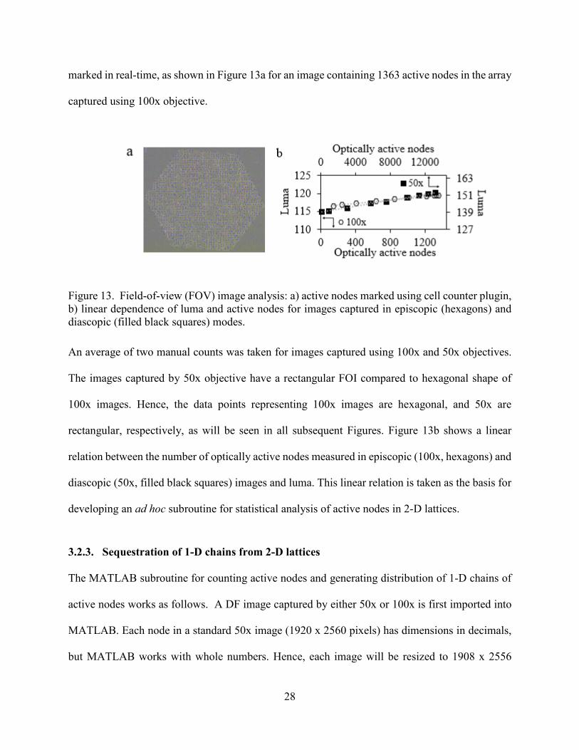
3.2.2. Manual tracking of optically active nodes ....................................................................... 27

3.2.3. Sequestration of 1-D chains from 2-D lattices ................................................................. 28

3.3. Detection of LPR and CLR resonances at differential fields-of-illumination (FOIs) ......... 30

3.3.1. Short-range illumination .................................................................................................. 30

3.3.1.1. Episcopic illumination: 60 μm FOI ............................................................................... 30

3.3.1.2. Diascopic illumination: 200 μm FOI ............................................................................ 33

3.3.2. Long-range illumination: ca.2000 μm FOI ...................................................................... 35

3.4. Comparisons of optical behavior of 2-D arrays characterized empirically, with theoretical

simulations .................................................................................................................................... 36

3.4.1. Single AuNP (Mie theory) versus AuNP array (present work) ....................................... 37

3.4.2. CDA versus experimental results ..................................................................................... 39

3.5. Summary ............................................................................................................................. 43

4. OPTO-THERMAL CHARACTERIZATION OF 2-D ARRAYS ................................... 44

4.1. Experimental measurements of optothermal responses of 2-D arrays at λLPR, λvalley, and

λCLR 45

4.2. Finite element modeling (COMSOL) ................................................................................. 71

4.3 Summary ................................................................................................................................. 79

5. SPECIAL PROPERTIES OF 2-D ARRAYS AND THEIR APPLICATIONS .............. 81

5.1. Complex systems, emergence, and critical point of emergence ......................................... 81

5.2. Applications of 2-D arrays .................................................................................................. 84

5.2.1. Plasmonic pervaporation for biofuel recovery ................................................................. 84

5.2.2. Ordered 2-D AuNP arrays and transition metal dichalcogenide (TMD) heterostructures85

5.2.3. Nanopore fabrication via dielectric breakdown for biosensing ....................................... 88

5.3. Summary ............................................................................................................................. 88

6. CONCLUSIONS AND FUTURE DIRECTIONS ........................................................................................... 90

6.1 Summary ............................................................................................................................................................................. 90

6.2 Future Directions .............................................................................................................................................................. 91

REFERENCES................................................................................................................................................................ ....... 92

LIST OF FIGURES Figure 1. Electron cloud oscillations in plasmonic NPs induced by light with wave vector k and

electric field E. ........................................................................................................................ 3

Figure 2. a) 20x dark field (DF) microscope image (scale bar: 50 μm) of the sample with its

corresponding LSPR response in the inset, and b) shows an SEM image of random AuNPs

of sizes 20-50 nm (scale bar: 2 μm). ....................................................................................... 4

Figure 3. 2-D array (100 μm x74 μm) with 13223 filled AuNP sites and 700 nm lattice spacing;

inset shows the extinction spectrum of the array with CLR and LPR peaks at ca.725 and

ca.560, respectively. ................................................................................................................ 5

Figure 4. Constructive and destructive interference in a square lattice with periodic, center-to-

center spacing ‘d’ between nodes (NP sites) under normal incidence of light that is x-

polarized. The diffractive modes in axial (green), diagonal (red) and OAD (violet) in the

upper right quadrant are illustrated with respect to a black node as a reference point. Nodes

separated by ‘2d’ are lighter in color. ..................................................................................... 6

Figure 5. Two-coupled harmonic oscillator system. ....................................................................... 7

Figure 6. An incident photon, |i⟩, can either excite a discrete resonance (|d⟩) with a coupling

factor w, or a continuum resonance (|c⟩) with a coupling factor g. A coupling strength v

forms between the discrete and continuum states. ................................................................ 10

Figure 7. PDMS-PEO stamps: a) PDMS-PEO glob (grey) dropped on pre-treated Si stamp

(black) placed on glass (blue), b) PDMS-PEO glob dropped on glass, c) Si stamp with

PDMS-PEO glob face-down d) PDMS-PEO sandwiched between Si stamp and glass, and e)

top view of the construct. ...................................................................................................... 18

Figure 8. Citrate- (left) and PVP-stabilized (right) AuNPs. ........................................................ 20

Figure 9. Evaporation-induced convection, and receding of contact line in a drop of water

(AuNPs) on PDMS-PEO and cover slip (dashed) with corresponding contact angles of 47°

and 61°, respectively. ............................................................................................................ 21

Figure 10. Template-assisted self-assembly: Case (a) t1 s shows the addition of 40 μL PVP-

stabilized AuNP solution onto PDMS-PEO with excess walls; t2 s shows wavefront

transport due to evaporation driven convection; t3 s shows liquid bridge breakup into into

satellite drops. Case (b) t1 s shows addition of 1-2 μL citrate-stabilized AuNPs on PDMS-

PEO; t2 s shows shrinkage of the drop due to evaporation; t3 s shows liquid bridge breakup

upon prolonged evaporation. ................................................................................................ 21

Figure 11. Mechanism of episcopic (left) and diascopic (right) modes of an optical microscope.

............................................................................................................................................... 25

Figure 12. Illustration of Young-Helmholtz theory, and the trichromacy principle of human

vision (LMS cones). .............................................................................................................. 26

Figure 13. Field-of-view (FOV) image analysis: a) active nodes marked using cell counter

plugin, b) linear dependence of luma and active nodes for images captured in episcopic

(hexagons) and diascopic (filled black squares) modes. ....................................................... 28

Figure 14. Working mechanism of the MATLAB subroutine: a) resized episcopic (100x) image,

b) extraction of R’G’B’ values for all pixels, c) luma pixel matrix generation, d) luma nodal

matrix generation, e) binary matrix generation, summation of total active nodes, and

sequestration of 1-D chains of varying sizes, and f) output containing distribution of 1-D

chain sizes of continuous active nodes. ................................................................................ 29

Figure 15. a) LPR (maxima at 540-560 nm) and CLR (maxima at 720-740 nm) magnitudes

increased with increasing number of active nodes in the FOI (148 to 1363). Spectra

(counts) were obtained at 100x magnification in episcopic illumination; b) Series of

corresponding DF images (a to j) of the lattice. .................................................................... 31

Figure 16. Distribution of chain sizes for sample areas captured with 100x containing active

nodes in the range 148-1363. ................................................................................................ 32

Figure 17. a) CLR and b) LPR features are plotted with the median chain size for each image

captured in episcopic mode, 100x (hexagons). Increasing particle median chain size gave

rise to higher intensities for both LPR and CLR features. .................................................... 33

Figure 18. a) LPR (maxima at 540-560 nm) and CLR (maxima at 720-740 nm) magnitudes

increased with increasing number of active nodes in the FOI (148 to 1363). Spectra (AU)

were obtained at 50x magnification in episcopic illumination; b) Series of corresponding DF

Images (a) to (g) of the lattice. .............................................................................................. 34

Figure 19. Long-range illumination: a) Samples a-e with ca.2 x 2 mm to ca.3 x 3 mm areas of

ordering, b) iridescence observed commonly on samples, and c) glimpse of 20x FOIs as

observed through the eyepiece. ............................................................................................. 35

Figure 20. SEM images of AuNPs transferred to glass: a) 2 μm, b) 1 μm. .................................. 36

Figure 21. Comparison of extinction in absorbance units of a 2-D array (13223 active nodes)

with Mie theory result for a single NP in extinction cross section (cm2). ............................ 38

Figure 22. CDA simulation of arrays with increasing sizes (5x5 to 30x30)................................. 40

Figure 23. Experimental versus simulations: a) rsa-CDA for AuNP arrays (present work, filled

black triangles), b) CDA and T-matrix for AgNP 1-D chains simulated by Zou et al.87

(hollow circles). The inset shows a power-law dependence between active nodes and CLR

magnitudes from episcopic (100x, hexagons) and diascopic (50x, filled squares) images. . 41

Figure 24. LPR increased linearly with increase in optically active nodes for a) episcopic (100x,

hexagons), and b) diascopic images (50x, filled black squares). .......................................... 42

Figure 25. White light source set-up comprising of a white light source, lens, removable power

trap, polarizer, neutral density filter, tunable filter, sample held by a 3-axis positioner and IR

camera for irradiating 2-D arrays at λLPR, λvalley and λCLR. ................................................... 44

Figure 26. Extinction spectra (AU) of Samples a-to-e captured using white-light source

illumination set-up. ............................................................................................................... 48

Figure 27. Extinction/NP for 2-D arrays (100 nm- filled green circles at λLPR and filled grey

triangles at λCLR) compared with random dispersions of AuNPs (16 nm-filled violet

diamonds, 76 nm-open violet diamonds, and 100 nm-filled yellow diamonds) in relation to

a) number of NPs per unit area (cm2), and b) number of NPs per unit deposition area (cm2).

............................................................................................................................................... 49

Figure 28. Mie theory plots of absorption, scattering and extinction cross sections for 16 nm, 76

nm, and 100 nm AuNPs. ....................................................................................................... 51

Figure 29. Extinction/NP for 2-D arrays (100 nm- filled green circles at λLPR and filled grey

triangles at λCLR) compared to random dispersions of AuNPs (16 nm-filled violet diamonds,

76 nm-open violet diamonds, and 100 nm-filled yellow diamonds) in relation to number of

NPs. ....................................................................................................................................... 52

Figure 30. Decrease of incident power (mW) with increase in wavelength. ................................ 54

Figure 31. Comparison of thermal responses from different systems in terms of a) ΔT / incident

intensity, and b) ΔT / (incident intensity * % Au). Films irradiated with white light were 2-

D arrays (filled green circles; 0.014 % to 0.096 %), and random dispersions containing NPs

such as 16 nm (filled violet diamonds; 0.001 % to 0.015 %), 76 nm (filled violet

diamond;0.005 %), and 100 nm (filled yellow diamond; 0.0066 %). Films irradiated with

laser are represented by red cross (Tagliabue et al.), blue asterisks (Li et al.), and black

crosses (Vanherck et al.). ...................................................................................................... 56

Figure 32.a) Experimental surface temperature plots (160 s heating) of Samples a-to-e at λLPR

where particle zones and ΔT calculation zones are enclosed with dashed and solid shapes

respectively, b) Thermal responses of 2-D arrays across λLPR (filled green circles), λvalley

(filled red squares), and λCLR (filled grey triangles; open grey triangles with Ge filter) in

comparison with random dispersions of 16 nm (filled violet diamonds), 76 nm (open violet

diamond, Ge filter), and 100 nm (filled yellow diamond, Ge filter) NPs. ............................ 58

Figure 33. Optics related to incident power, which is the sum of reflection, transmission, and

attenuation. Attenuation is further equal to the sum of scattering, diffraction, and absorption.

............................................................................................................................................... 61

Figure 34. a) Thermal responses in terms of extinguished intensity vs wavelength at λLPR, and b)

thermal responses in terms of absorbed, extinguished intensity vs wavelength at λLPR. 2-D

arrays are represented by filled green circles, whereas filled violet diamonds correspond to

16 nm dispersions, open violet diamond corresponds to 76 nm dispersions, and filled yellow

diamond corresponds to 100 nm dispersions. ....................................................................... 62

Figure 35. a) Thermal responses in terms of absorbed, extinguished intensity vs NPs per unit area

(cm2) at λLPR, and b) thermal responses in terms of absorbed, extinguished intensity vs NPs

per unit deposition area (cm2) at λLPR. 2-D arrays are represented by filled green circles,

whereas filled violet diamonds correspond to 16 nm dispersions, open violet diamond

corresponds to 76 nm dispersions, and filled yellow diamond corresponds to 100 nm

dispersions............................................................................................................................. 64

Figure 36. Experimental thermal profiles of Sample a (700 nm spacing, Type 2, Table 3) and its

respective control: a) heating-cooling curve of sample, b) equilibrium (160 s heating)

topographical temperature map of sample relative to this length and width (illuminated at

center-left), c) heating-cooling curve of control, and d) topographical temperature map of

control relative to this length and width (illuminated at center-left). ................................... 66

Figure 37. Experimental thermal profiles of Sample b (700 nm spacing, Type 2, Table 3) and its

respective control: a) heating-cooling curve of sample, b) equilibrium (160 s heating)

topographical temperature map of sample relative to this length and width (illuminated near

upper-left), c) heating-cooling curve of control, and d) topographical temperature map of

control relative to this length and width (illuminated near upper-left). ................................ 67

Figure 38. Experimental thermal profiles of Sample c (700 nm spacing, Type 2, Table 3) and its

respective control: a) heating-cooling curve of sample, b) equilibrium (160 s heating)

topographical temperature map of sample relative to this length and width (illuminated at

bottom-center), c) heating-cooling curve of control, and d) topographical temperature map

of control relative to this length and width (illuminated at bottom-center). ......................... 68

Figure 39. Experimental thermal profiles of Sample d (600 nm spacing, Type 1, Table 3) and its

respective control: a) heating-cooling curve of sample, b) equilibrium (160 s heating)

topographical temperature map of sample relative to this length and width (illuminated at

lower-left), c) heating-cooling curve of control, and d) topographical temperature map of

control relative to this length and width (illuminated at lower-left). .................................... 69

Figure 40. Experimental thermal profiles of Sample d (600 nm spacing, Type 1, Table 3) and its

respective control: a) heating-cooling curve of sample, b) equilibrium (160 s heating)

topographical temperature map of sample relative to this length and width (illuminated at

bottom left), c) heating-cooling curve of control, and d) topographical temperature map of

control relative to this length and width (illuminated at lower-left). .................................... 70

Figure 41. Thermal profiles obtained with Ge filter in light path: a) and b) show the heating-

cooling curves of 76 nm dispersion (0.005 %) and the corresponding control, respectively.

Similarly, c) and d) show the heating-cooling curves of 100 nm dispersion (0.0066 %) and

the corresponding control, respectively. ............................................................................... 71

Figure 42. Temperature profile in a finite slab. The Legend shows dimensionless times. ........... 75

Figure 43. Surface temperature maps of Samples a-to-e generated using absorbed, extinguished

powers at λLPR. The COMSOL results are compared with experimental profiles at 160 s.

Dashed lines enclose particle areas. ...................................................................................... 76

Figure 44. Surface temperature maps of Samples a-to-e generated using fitted powers at λLPR.

The COMSOL results are compared with experimental profiles at 160 s. Dashed lines

enclose particle areas. Dotted lines enclose irradiation zones. ............................................. 77

Figure 45. Fitted vs actual absorbed, extinguished powers for Samples a-to-e in relation to a) T,

number of NPs, and sample area, and b) ΔT, number of NPs, and sample area .................. 78

Figure 46. Initial occurrence of LPR followed by evolution (dark blue arrow) of CLR (red

dashed box), and involution (light blue arrow) of CLR (ca. 775 nm) and LPR peaks. ........ 84

LIST OF TABLES Table 1. Template-assisted self-assembly methods involving capillary and/or convective forces.

15

Table 2. Figure of merits for template-assisted methods listed in Table 1. 16

Table 3. Lattice configurations. 19

Table 4. Commonly occurring spatial conformations of NP ensembles inside a cavity. 19

Table 5. Experimental conditions and outcomes for five samples produced using Case b. 23

Table 6. Sample dimensions. 52

Table 7. Lattice configurations of Samples a-to-e. 52

Table 8. Au mass concentrations in 2-D arrays (Samples a-to-e) and random dispersions 53

NOMENCLATURE

Chemical Symbols, Acronyms, and Abbreviations Ag Silver Au Gold AU Absorbance Units AuNP Gold Nanoparticle BF Bright Field CDA Coupled Dipole Approximation CLR Coupled Lattice Resonance CVD Chemical Vapor Deposition DDA Discrete Dipole Approximation DF Dark Field DI Deionized Water DNA Deoxyribonucleic Acid EBL Electron Beam Lithography EELS Electron Energy Loss Spectroscopy EL Electroless plating EUV-IL Extreme Ultraviolet Interference Lithography FIB Focused Ion Beam FGMS Fixed Glass and Mobile Substrate FOI Field-of-Illumination

FOV Field-of-view Ge Germanium HCI Hot Carrier Injection HER Hydrogen Evolution Reaction IR Infrared ITU International Telecommunion Union LMS Long, Medium, and Short Wavelengths of Light LPR Lattice Plasmon Resonance LSPR Localized Surface Plasmon Resonance MoS2 Molybdenum Disulfide MoSe2 Molybdenum Diselenide NIL Nanoimprint Lithography NIR Near-Infrared NP Nanoparticle NSL Nanosphere Lithography 1-D One-Dimensional PDMS Polydimethylsiloxane PDMS-b-PEO Poly(dimethylsiloxane-b-ethyleneoxide) PDMS-PEO Poly(dimethyloxane-ethyleneoxide) PH Peak Height

Pt Platinum RGB Red, Green, and Blue (Linear Form) R’G’B’ Red, Green, and Blue (Non-Linear Form) ROI Region of Interest rsa-CDA Rapid Semi-Analytical Solution, Coupled Dipole Approximation SEM Scanning Electron Microscopy SHG Second Harmonic Generation SiO2 Silicon Dioxide SPR Surface Plasmon Resonance TMD Transition Metal Dichalcogenide 2-D Two-Dimensional WS2 Tungsten Disulfide Symbols and Popular Units Interparticle Distance [nm] Eigenmode Frequency or Natural Frequency of the Oscillator [rad s-1] Linear Damping Coefficient [dimensionless] Amplitude of the External Force [units vary] or Radius of the Sphere [nm]

Steady-State Amplitude of the Oscillator [units vary] Coupling Factor [dimensionless] or Kinematic Viscosity of the fluid [m2 s-1] Phase Shift [rad] Incident Photon [dimensionless] Continuum State [dimensionless] Discrete State [dimensionless] Excitation Probability Ratio[dimensionless] or Heat Flux [W m-2] Coupling Factor Corresponding to Discrete State [dimensionless] Coupling Factor Corresponding to Continuum State [dimensionless] or Acceleration Due to Gravity [m s-2] Reduced Energy [eV], Electric Permittivity [F m-1], or Emissivity of the material [dimensionless] Energy of Incident Photon [eV] or Incident Field [V m-1] Line width [nm] Luma or Photometric Brightness [dimensionless] Cross Section [m2] or Stefan-Boltzman Constant [~5.67e-8 W m-2 K-4] Polarizability [C m2 V-1] or Thermal Diffusivity of the

Fluid [m2 s-1] Efficiency [dimensionless] Polarization [C m-2] Retarded Dipole Sum [dimensionless] Wavevector [rad per unit distance] or Thermal Conductivity [W m-1 K-1] Density of the Material [Kg m3] Specific Heat Capacity of the Material [KJ K-1] Temperature [K] n Normal vector to the film surface [dimensionless] Del Operator [dimensionless] t Time [s] Total Heat Sources or Sinks [W m-2] Heat Transfer Coefficient [W m2 K-1] Plate Height [m] Rayleigh Number [dimensionless] Prandtl Number [dimensionless] Coefficient of Thermal Expansion [K-1] Dimensionless Temperature η Dimensionless Distance Length of the Slab [m]

Subscripts

Initial Condition

Plasmon (Continuum Resonance) or

Specific Heat Capacity

Discrete Resonance

Modified Line Width of Discrete Resonance

Absorption, Scattering, or Extinction

Specific Temperature Value

Ambient temperature of the Fluid

Incident Field Superscript(s)

’ Non-Linear Representation of Luma

1

1. INTRODUCTION

This chapter primarily focuses on the motivation for the present work, and introduction of plasmon

and Fano dual-resonances. Models pertaining to classical and quantum physics will be introduced

that describe these dual-resonances in metamaterial arrays. This chapter finally ends by

enumerating key advances of the present work, and an overall summary.

1.1 Motivation

1.1.1. Sustainable energy

Population explosion in the last 60 years led to an increased demand of global energy.1,2 According

to a recent estimate, power consumption in 2050 would be around 30 TW compared to 17 TW

today which would correspond to a 1.7-fold increase.3 Primary sources of energy, i.e., fossil fuels

have already been on the verge of decline. Conversely, coal reserves will remain intact for a long

time;4 nevertheless, both fossil fuels and coal contributed largely to greenhouse effect (carbon

dioxide emissions) resulting in global warming.5 In 2015-16, world economies agreed upon two

important sets of goals for future considering the current environmental conundrums: Sustainable

Development Goals and the Paris Agreement on Climate Change action for phasing out fossil fuels

by 2100.6 Sustainable energy for: supporting escalating demands of growing population,

complementing ecological balance, and reducing waste heat is imperative in the current global

scenario.

Sustainable energy sources such as wind,7 geothermal,8 solar,9 fuel cells10 and biofuels11 have

already been on the rise for the past 50 years.12 A crossover between plasmonics and photonics in

recent decades paved the path for utilization of plasmonic nanomaterials for progressive

advancement of some of these systems at the lab scale. Specific examples include augmentation

2

of electron-hole pairs, i.e., excitons (and photocurrent) in solar photovoltaics,13 and efficient

catalytic activity in fuel cells.14 However, challenges pertaining to ohmic losses limit the

performance of these plasmonic systems.15,16 This work focuses on thermalization aspects of

plasmonic nanomaterials arranged into two-dimensional (2-D) arrays in polymer media, and

implementation of such systems for applications requiring enriched energy dissipation.

1.1.2. Healthcare

Viable interactions of biological substances such as peptides, deoxyribonucleic acid (DNA),

antigens, and oligonucleotides with functionalized nanomaterials via ligand transfer, covalent

bonding or passive adsorption has resulted in unique applications of plasmonic nanomaterials in

therapeutics, point-of-care diagnostics, anti-bacterial activity, ablation of cancer cells, and drug

delivery.17–23 For example, energy exchange between conductive nanoparticles (NPs) and redox

proteins (e.g. cytochrome) supports development of amperometric biosensors wherein redox

enzymes act as sensing entities, and NP arrays function as the conductive matrix onto which the

enzyme molecules adhere.17 The changes in surrounding dielectric due to external

biomolecules/biological specimens affect the overall system-sensitivity in tandem with opto-

thermal responses of such arrays.17,20 Understanding the dynamic energy exchange pathways in

these systems vis-à-vis plasmonic dissipation and thermal changes due to ‘diffractive coupling’ in

NP arrays is imperative for further advancement of these nano-bio-photonic systems.

1.2. Background

1.2.1. Plasmon resonance

Surface plasmon resonance (SPR) is a surface phenomenon where conduction electrons in noble

metals such as gold (Au), silver (Ag), and platinum (Pt) collectively oscillate at a resonant

3

frequency of the incident light. Unlike metallic surfaces, NPs owing to a large-surface area-to-

volume ratio (ca.107:1 ratio for a 10 nm NP compared to a regular cricket ball) have an exceptional

tendency to scatter and absorb light. Geometric confinement of plasmons at the metal-dielectric

interface of a NP leads to a localized surface plasmon resonance (LSPR), which is dependent on

particle shape, size, and the surrounding dielectric environment.24–29 Figure 1 schematically shows

formation of dipoles in NPs due to a light wave with wavevector 𝑘𝑘 propagating from left to right

with an orthogonal electric field (y-polarization).

Figure 1. Electron cloud oscillations in plasmonic NPs induced by light with wave vector k and electric field E.

As the LSPR decays, excited electron cloud couples with phonons, or crystal lattice vibrations,

resulting in an increase in thermal energy. This thermal energy is eventually dissipated to the

surrounding environment via phonon-phonon interactions.30–32 Thermoplasmonic heating in NPs

induced by electromagnetic radiation has been used for applications pertaining to solar

photovoltaics and healthcare, as outlined in the preceding sections, and advancements in

microelectronics for over 50 years which led to the progressive increase in computing power at

decreased relative costs (Moore’s law).33 Figure 2a (inset), for example, shows the extinction

response in absorbance units (AU) of a random ensemble of AuNPs on soda lime glass (Figures

4

2a and 2b) deposited via tin pre-sensitization on glass and electroless (EL) plating of AuNPs.34

The maxima of the LSPR occurred at ca. 560 nm.

Figure 2. a) 20x dark field (DF) microscope image (scale bar: 50 μm) of the sample with its corresponding LSPR response in the inset, and b) shows an SEM image of random AuNPs of sizes 20-50 nm (scale bar: 2 μm).

1.2.2. Fano resonance (coupled lattice resonance)

Italian-American physicist Ugo Fano was the pioneer in exploring asymmetric peaks arising from

coupling between a discrete resonance and a broadband resonance. 35 Fano resonances can be

observed in many areas of physics and engineering. The focus of this work is to describe the Fano

resonance occurring in 2-D arrays. AuNPs ordered into 2-D arrays support coupling of a plasmon-

enriched local electromagnetic field to diffracted light, resulting in a coupled lattice resonance

(CLR)/Fano resonance. For example, Figure 3 shows a 2-D array (100 μm x74 μm) of 13223 sites

filled with AuNPs, and 700 nm lattice spacing (grating constant). The inset shows the extinction

peak of the array, where CLR feature appears at ca.725 nm due to periodic arrangement in addition

to a lattice plasmon resonance (LPR) feature that appears at ca. 560 nm. Note that the CLR feature

was absent in the inset of Figure 1a for random ensembles.

5

Figure 3. 2-D array (100 μm x74 μm) with 13223 filled AuNP sites and 700 nm lattice spacing; inset shows the extinction spectrum of the array with CLR and LPR peaks at ca.725 and ca.560, respectively.

The LPR and CLR features can be generally tuned in relation to the polarization of the incident

electromagnetic field,36 grating constant,37 NP geometry28,29, and refractive index of the medium.38

This work particularly shows important effects of particle density on the intensity of LPR and

CLR features.

Figure 4 schematically illustrates a square lattice of NP sites (nodes) subjected to orthogonal

incidence (into the plane) of light with x-polarization. The periodic, center-to-center spacing

between the nodes is d. The diffractive modes in the upper right-hand quadrant are shown vis-à-

vis a reference black node at the center. Nodal elements in axial (y-axis), and diagonal (y=x) are

green and red, respectively. Remaining nodes in off-axial and off-diagonal (OAD) directions are

violet. Nodes separated by 2d are lighter in color than their counterparts at a spacing ‘d’ within a

6

chain of each diffractive mode. Constructive and destructive interferences are illustrated with

respect to the direction of wave propagation.

Figure 4. Constructive and destructive interference in a square lattice with periodic, center-to-center spacing ‘d’ between nodes (NP sites) under normal incidence of light that is x-polarized. The diffractive modes in axial (green), diagonal (red) and OAD (violet) in the upper right quadrant are illustrated with respect to a black node as a reference point. Nodes separated by ‘2d’ are lighter in color.

Nodes present along the direction of polarizability (x-axis) are not conducive to far-field

diffraction coupling, as dipoles do not radiate along their dipole moment.39,40 Square lattices (𝑑𝑑𝑥𝑥 =

𝑑𝑑𝑦𝑦) represent a special case of rectilinear lattices and exhibit 𝜋𝜋/2 rotational symmetry for an

isotropic response to x- and y-polarization. The present work primarily considered far-field

diffractive coupling effects from square lattices. Far-field effects are predominant, with a

dependence of d-1, when the interparticle distance (d) is greater than the size of the NP, and near

or above LSPR wavelength (λLSPR) of the NP. Near-field interactions dominate and show a d-3

dependence as the interparticle distance decreases to dimensions comparable to NP size. 41,42

7

Two models pertaining to classical and quantum-mechanical theories of dual-resonant systems

were reported in literature, which have an important relevance to the present work. The following

discussion will focus on the illustration of these models.

Systems exhibiting dual-resonances has been famously expounded by the classical model of

harmonic oscillators.43 Consider two oscillators coupled by a weak spring, as shown in Figure 5,

where and external force is driving oscillator 𝜔𝜔1.

Figure 5. Two-coupled harmonic oscillator system.

The equations of motion for these oscillators may be written as:

��𝑥1 + 𝛾𝛾1��𝑥1 + 𝜔𝜔12𝑥𝑥1 + 𝑣𝑣12𝑥𝑥2 = 𝑎𝑎1𝑒𝑒𝑖𝑖𝑖𝑖𝑖𝑖 (1.1)

��𝑥2 + 𝛾𝛾2��𝑥2 + 𝜔𝜔22𝑥𝑥2 + 𝑣𝑣12𝑥𝑥1 = 0 (1.2)

where 𝜔𝜔1 and 𝜔𝜔2 are the natural frequencies/eigenmodes of oscillators, 𝛾𝛾1 and 𝛾𝛾2 are linear

damping coefficients, 𝑣𝑣12 corresponds to the coupling of oscillators, ω is the external driving

frequency, and 𝑎𝑎1 is the amplitude of the external driving force.

8

The coupling term is zero in the event of no external force acting on the system, i.e., oscillators

swing independently according to their natural frequencies. But coupled oscillators have two

normal modes (eigenmodes): a) oscillators swing to and fro together, and b) oscillators swing in

opposite directions. The coupled eigenmodes in this system are expressed as follows:

where ω�1 and ω�2 are the displaced eigenmodes due to the coupling between oscillators. The

amplitudes for these oscillators from the steady-state harmonic solutions of Equations 1.1 and

1.2 are:

𝑐𝑐1 =𝜔𝜔22 − 𝜔𝜔2 + 𝑖𝑖𝛾𝛾2𝜔𝜔

(𝜔𝜔12 − 𝜔𝜔2 + 𝑖𝑖𝛾𝛾1𝜔𝜔)(𝜔𝜔22 − 𝜔𝜔2 + 𝑖𝑖𝛾𝛾2𝜔𝜔) − 𝑣𝑣122𝑎𝑎1 (1.5)

𝑐𝑐2 =𝑣𝑣12

(𝜔𝜔12 − 𝜔𝜔2 + 𝑖𝑖𝛾𝛾1𝜔𝜔)(𝜔𝜔22 − 𝜔𝜔2 + 𝑖𝑖𝛾𝛾2𝜔𝜔) − 𝑣𝑣122𝑎𝑎1 (1.6)

where c1, and c2 are the steady-state amplitudes for these oscillators. The phases of the two

oscillators are defined by:

𝑐𝑐1(𝜔𝜔) = |𝑐𝑐1(𝜔𝜔)|𝑒𝑒−𝑖𝑖𝜑𝜑1(𝑖𝑖)

𝑐𝑐2(𝜔𝜔) = |𝑐𝑐2(𝜔𝜔)|𝑒𝑒−𝑖𝑖𝜑𝜑2(𝑖𝑖)

(1.7)

(1.8)

where the phase difference and phase shift (𝜃𝜃) are given as:

𝜑𝜑2 − 𝜑𝜑1 = 𝜋𝜋 − 𝜃𝜃 (1.9)

𝜃𝜃 = 𝑡𝑡𝑎𝑎𝑡𝑡−1 �𝛾𝛾2𝜔𝜔

𝜔𝜔22 − 𝜔𝜔2� (1.10)

𝜔𝜔�12 ≈ 𝜔𝜔12 −

𝑣𝑣122

𝜔𝜔22 − 𝜔𝜔12 (1.3)

𝜔𝜔�22 ≈ 𝜔𝜔22 +

𝑣𝑣122

𝜔𝜔22 − 𝜔𝜔12 (1.4)

9

Increasing the coupling factor, 𝑣𝑣12, diminishes the coupled eigenmode frequency of oscillator 1,

𝜔𝜔�12 (Equation 1.3), and causes a red-shift in wavelength (due to a reciprocal relation between

frequency and wavelength). But eigenmode frequency of oscillator 2, 𝜔𝜔�22 (Equation 1.4), would

increase showing a concomitant blue-shift in wavelength. Imagine a simplest case when the

frictional parameter (damping coefficient), 𝛾𝛾1, is zero from Equation 1.5. When an external force

drives the frequency of the first oscillator close to that of the second oscillator, 𝑐𝑐1 becomes zero.

This frequency is referred to as zero-frequency, which induces an asymmetric profile that is

commonly associated with a small dip. 43 This model could be primarily used to understand the

energy shifts associated with coupling between continuum (plasmon) and discrete (lattice

diffraction) states of square lattices.

A quantum mechanical equivalent of classical model was reported recently that delves deeper into

the nature of continuum and discrete resonances in terms of three coupling factors.44,45 Imagine a

system where an incident photon, |𝑖𝑖⟩, excites either a continuum state (|𝑐𝑐⟩) with coupling factor 𝑔𝑔,

or a discrete state (|𝑑𝑑⟩) with coupling factor 𝑤𝑤. Also, continuum and discrete states interact with a

certain coupling strength 𝑣𝑣. Equation 1.11 represents the Fano profile of this system where 𝜀𝜀 is

the reduced energy, and 𝑞𝑞 is the excitation probability ratio (asymmetry parameter):

𝐹𝐹(𝜀𝜀) = (ℰ+𝑞𝑞)2

ℰ2+1 (1.11)

Equation 1.12 represents 𝑞𝑞 in terms of 𝑣𝑣, 𝑤𝑤, and 𝑔𝑔, energy of the incident photon (𝐸𝐸), plasmon

energy (𝐸𝐸𝑝𝑝), plasmon linewidth (Г𝑝𝑝), and modified linewidth of the discrete resonance, Г𝑚𝑚(𝐸𝐸),

with an energy of (𝐸𝐸𝑑𝑑):

q= 𝑣𝑣𝑣𝑣/𝑔𝑔Г𝑚𝑚(𝐸𝐸)/2

+ 𝐸𝐸−𝐸𝐸𝑝𝑝Г𝑝𝑝/2

(1.12)

The reduced energy (𝜀𝜀) may be written as:

10

ε= 𝐸𝐸Г𝑚𝑚(𝐸𝐸)/2

+ 𝐸𝐸−𝐸𝐸𝑝𝑝Г𝑝𝑝/2

(1.13)

Equations 1.14 shows the relation between the modified linewidth of discrete state and

Lorentzian profile of plasmon resonance (Equation 1.15):

Г𝑚𝑚(𝐸𝐸) = 2𝜋𝜋𝑣𝑣2L (𝐸𝐸) (1.14)

L (𝐸𝐸) = 1

1+(𝐸𝐸−𝐸𝐸𝑝𝑝Г𝑝𝑝/2 )2

(1.15)

The important insight that can be gained from this analytical model is that there is a probability to

excite either a discrete state (𝑤𝑤) or a continuum state (𝑔𝑔) first by an incident photon, and these

resonances interact via a coupling strength (𝑣𝑣).44,45 Figure 6 illustrates the essence of this model,

where the putative discrete resonance is shown by a sharp profile (𝒒𝒒𝟐𝟐−𝟏𝟏𝓔𝓔𝟐𝟐+𝟏𝟏

), and continuum resonance

follows a flat profile (1). The mixing condition is represented by 𝒒𝒒𝟐𝟐−𝟏𝟏𝓔𝓔𝟐𝟐+𝟏𝟏

. The resultant Fano profile

is generally represented as shown in Equation 1.11. 35,46

Figure 6. An incident photon, |i⟩, can either excite a discrete resonance (|d⟩) with a coupling factor w, or a continuum resonance (|c⟩) with a coupling factor g. A coupling strength v forms between the discrete and continuum states.

11

1.3. Key advances of the present work

The significant advances made in this study are:

1. Creation of 2-D metamaterial arrays using template-assisted self-assembly via

modification of polydimethylsiloxane (PDMS) with poly (dimethylsiloxane-b-ethylene

oxide) (PDMS-b-PEO).

2. Opto-thermal characterization of 2-D metamaterial arrays in visible as well as near-

infrared (NIR) wavelengths.

3. Energy dissipation from 2-D arrays at CLR resonances (NIR) in addition to plasmon

reosnances (visible).

4. Extension of three-dimensional (3-D) slab model (COMSOL) for embedded NPs into a

dual-slab model (2-D lattices on a film)

5. Implementation of an all-optical approach that includes image analysis and statistical

analysis for characterizing metamaterial arrays.

1.4. Summary

Integration of plasmonics with photonics paved the path for key research opportunities for

advancement of sustainable energy and healthcare systems. Enhanced energy generation due to

plasmon-photon interactions could result in economies of scale in the long-run concerning

production of biofuels, or order-of-magnitude increases in electron-hole pair generation and

photocurrent in solar photovoltaics. Plasmonic/photonic metamaterials with augmented opto-

thermal responses and energy dissipation pathways could be used for diagnosing biological

molecules, direct thermal ablation of cancer cells, drug delivery, etc. Particularly, 2-D

metamaterial arrays which exhibit diffractive coupling as a result of interaction of lattice

diffraction with plasmons can be used to provide alternate energy dissipation pathways. The

12

concept of plasmon and Fano coupled lattice resonances (CLR) in 2-D arrays has been delineated

in detail by considering deep-rooted models of Physics: classical analogy of harmonic oscillators

and quantum-mechanical analytical model. Key advances in the present work have been

enumerated, which will be discussed in detail in ensuing chapters.

13

2. FABRICATION OF 2-D ARRAYS

This chapter deals with traditional methods for fabrication of 2-D arrays, template-assisted self-

assembly methods discussed in literature thus far, soft lithography for creating nanoimprinted

PDMS-PEO square lattices, and variations of template-assisted self-assembly for depositing

AuNPs in the cavities of PDMS-PEO lattices used in the present work.

2.1. Fabrication methods

Some of the traditional methods for creating 2-D arrays are listed as follows:

a) Electron beam lithography (EBL) allows intricate, user-defined patterning through

lithography of a polymeric resist by an electron beam.47,48

b) Focused ion beam (FIB) entails milling of substrates using gallium (Ga) ion beams and

offers high precision.49,50

c) Nanosphere lithography (NSL) involves masking of a substrate during metallization using

colloidal spheres, where sphere dimensions govern the lattice spacing.51,52

d) Nanoimprint lithography (NIL) exploits a master image pre-lithographed using

electron/ion beam or interference to mold template patterns onto substrates using resists.53–

55

e) Soft lithography uses a pre-lithographic master stamp created by one of these top-down

approaches to pattern a PDMS polymer. The negative geometry of the master is transferred

to the polymer. Soft lithography is commonly used for applications involving

microfluidics.56,57

14

2.2. Template-assisted self-assembly

2-D arrays of NPs could be produced inexpensively using bottom-up methods compared to top-

down methods using self-assembly techniques such as colloidal/nanosphere lithography,51,52,58 and

template-assisted self-assembly.59–64 Template-assisted self-assembly, in particular, has recently

gained interest, owing to its economic viability and efficacy over other self-assembly techniques

that depend on interfacial and inter-particle forces. Additionally, customized templates allow

leverage over dense packing of NPs.60 Chemical functionalization and topographical patterning of

substrates is commonly employed for homogeneous distribution of forces that guide the particles

to periodic cavities with special geometrical shapes. Packing density of cavities and overall lattice

spacing could be tunable for multivalent applications. Commonly exploited forces/processes in

template-assisted self-assembly are electrostatic, magnetic, convection, capillary, sedimentation,

host-guest interactions, etc.

Table 1 summarizes template-assisted self-assembly techniques which were based primarily on

capillary and convective forces. These techniques can be further grouped into two types: a) solvent

enclosed between a fixed glass and mobile substrate (FGMS), and b) dip coating, where a template

is immersed in a NP suspension.

15

Table 1. Template-assisted self-assembly methods involving capillary and/or convective forces.

Substrate Templating method

Treatment NP (size, nm)

NPs/mL Cavity (holes) (nm)

Parameters Self-assembly Vs d

(μm/s)

Ts e (˚C)

PDMS bilayer59

Soft-lithography

O2 plasma (substrate)

Au (88) 3e+10 Da=580 Hb=140

Pc=1300-1400

0.6 21 FGMSf

PDMS60

Soft-lithography

O2 plasma (substrate)

Au (100) 5.6e+9 (Au) D=120 H=80

0.2 28 FGMS

Mylar films61

Photo-lithography

none PS beads (700-4300)

NA g D=2000-6000

H=2000-5500

0.3 NA FGMS

PMMA on Cr/SiO2-Si62

EUV-IL none Au (15-50); Si (45-50)

4.5e+10 -1.7e+14

(Au); 4.3e+11-

4.3e+14 (Si)

P=70-115

0.5 NA

Dip coating

SiOx layer on top of

Si63

EBL none Au (50) 4.5e+10 D=50- 110

H=ca.60

0 60 Dip coating

PDMS64

Soft-lithography

Triton X-45 and dodecyl

sulphonate (surfactant for

colloidal suspension)

Au (60-100) 2e+11 H=40-45 Pf=280-

1000

0.3 27 FGMS

Present work Soft-lithography

PEO (substrate)

Au (80-100) 1e+8-1e+9 D=195-260

H=150-350

P=600-700

0 25 FGMS

a diameter; b height; c pitch; d substrate/dip velocity; e substrate temperature; f solvent trapped between a fixed glass and movable substrate; g not available

Especially, the FGMS technique entails moving a substrate on motorized platforms at low

velocities. Evaporation-induced convective transport of solvent in conjunction with capillary

forces support NP depositions into cavities near the receding contact line of solvent. Substrate

velocity in μm/s, and substrate temperature can be controlled relative to NP volume to obtain

ordered NP deposition. Dip coating, on the other hand, involves substrate immersion in a NP

suspension. The dip velocity, NP concentration and solvent temperature can be tuned to monitor

the deposition process. Templates of diverse materials such as mylar films, PDMS, and SiOx have

16

been used in these techniques. In particular, PDMS has been widely used owing to its extensive

applications in microfluidics.

The present work led to the design and fabrication of 2-D arrays based on FGMS technique. In

contrast to intricate methods such as extreme ultraviolet interference lithography (EUV-IL), EBL

and FIB, soft-lithography was used to create templates comprised of PDMS and PEO for the self-

assembly process.

Table 2 shows the figures of merit of template-assisted methods listed in Table 1. Varying the

concentration of NP solvent, and lattice configuration permitted formation of NP ensembles with

varying spatial conformations (monomers to heptamers) in FGMS systems. Ensemble types

ranging from monomers to dodecamers were reported with assorted lattice geometries in dip

coating. Cluster yields varied from 32% (PDMS) to 90% (mylar).

Table 2. Figure of merits for template-assisted methods listed in Table 1.

Ensemble Conformations Yield (%)

Characterization Method

Optical Resonances

Heptamers59

32 (PDMS) SEM Plasmon and

Fano Monomers60 NA SEM NA

Monomer, dimers, trimers, tetramers, pentamers61

ca.90 (mylar) SEM NA

Monomers at interstitial sites62

NA SEM NA

Monomers63 NA SEM NA Monomers64 NA SEM NA

Characterization methods mostly involved analyzing ensembles with SEM. The proposed work

includes alternate characterization methods such as diascopic and episcopic microscopy and image

analysis. Charging effects on an insulating surface such as PDMS due to electron imaging

techniques at high vacuum conditions may deteriorate the quality of images. Ultra-thin conductive

coating on PDMS for SEM was further avoided, as it may cause the opto-thermal responses of

samples to alter.

17

2.2.1. Enhancement of PDMS surface energy using PDMS-b-PEO copolymer

PDMS is fundamentally hydrophobic owing to a low surface free energy compared to water

(PDMS: 20 mN/m; water: 72 mN/m).65,66 Numerous techniques to increase the surface energy of

PDMS have been attempted previously such as sol-gel coatings, oxygen plasma, UV/ozone, layer-

by-layer deposition, chemical vapor deposition (CVD), etc.59,60,67,68 However, PDMS is resilient

to these treatments and recovers its hydrophobic nature eventually due to low glass transition

temperature (-120 ˚C).

PDMS-b-PEO diblock copolymer was used in the present work to rapidly increase the surface

energy of PDMS after mixing and curing steps with PDMS. Yao et al. 69 noted that the water

contact angles decreased from 100˚ to 20˚ (5-fold) upon increasing the concentration of PDMS-

PEO from 0% to 1.9%. Modulating the cross-linking density would allow further manipulation of

the wetting property of PDMS.70

2.2.2. Soft Lithography for creating nanoimprinted polymer templates

PDMS base with curing agent (Sylgard 184 silicone elastomer kit; #240 401 9862) was purchased

from Dow Corning Corporation (Midland, MI, U.S.A). A di-block copolymer of PDMS-b-PEO

(75:25), methyl terminated (#09780-100), from Polyscience Inc. (Warrington, PA, USA) was used

to make PDMS hydrophilic. The speed mixer (#DAC 150SP/601 0064) and its plastic containers

were purchased from FlackTek Inc. (Landrum, SC, USA).

The polymer mixture was prepared by mixing x mg PDMS-b-PEO, y mg of PDMS monomer and

y/10 mg of curing agent such that (x/y) * 100=2.07 % PDMS-b-PEO relative to PDMS monomer.

The contents of the container were mixed for 6 minutes at 3000 rpm. Then, a 20-60 mg glob of

PDMS-PEO (grey) was dropped on an iridescent Si master (black) and also on a 2.5 x 1 inch’s

rectangular glass slide (light blue) that had two 1 x 1 inch’s square glass mounts on its sides, as

18

schematically depicted in Figures 7a and 7b, respectively. The Si master was pre-rinsed with

acetone and deionized (DI) water, and dried with air. The Si master with the glob was then inverted

(Figure 7c) and placed on top of square mounts at a 45-degree angle (Figures 7d and 7e). The

construct was then degassed in a vacuum chamber at 25-30 mm Hg and placed on a hot plate at

45°-150° C. Cured PDMS-PEO templates were stored in polystyrene plastic boxes. Typical

thickness of PDMS-PEO stamps produced by this method are ca.300 μm.

Figure 7. PDMS-PEO stamps: a) PDMS-PEO glob (grey) dropped on pre-treated Si stamp (black) placed on glass (blue), b) PDMS-PEO glob dropped on glass, c) Si stamp with PDMS-PEO glob face-down d) PDMS-PEO sandwiched between Si stamp and glass, and e) top view of the construct.

19

Table 3 enumerates the geometric configuration of PDMS-PEO templates negatively imprinted

from Si master with posts.

Table 3. Lattice configurations.

Dimensions [nm] Type 1 Type 2 Type 3 Lattice pitch 600 700 700 Cavity depth 150 150 350 Cavity diameter 195 260 260

Table 4 shows monolayer spatial confirmations of spherical NPs that can fit inside a PDMS-PEO

cylindrical cavity (top view) based on the ratio of diameter of the cavity to diameter of the

particle.61

Table 4. Commonly occurring spatial conformations of NP ensembles inside a cavity.

Two types of AuNPs were used in the current work: a) AuNPs with polyvinlypyrrolidone (PVP)

shell that are stable due to steric stabilization in solutions, and b) citrate-stabilized AuNPs which

20

are stable due to electrostatic repulsions resulting from negatively charged citrate ions.71 The

citrate and PVP capping agents around NP surfaces are shown in Figure 8 schematically.

Figure 8. Citrate- (left) and PVP-stabilized (right) AuNPs.

2.2.3. Particle deposition via evaporative convection

Figure 9 schematically shows NPs (yellow) in a water drop on PDMS-PEO (grey), where the

estimated contact angle was 47°. Additionally, the contact angle estimated for a water drop

(dashed) on borosilicate cover slip (blue) was 61°. Due to evaporation (red arrows) of solvent at

the interface, capillary forces drive particles at the center to the interface (indicated by green

arrows). The contact line at the interface recedes continuously, thereby pinning the particles onto

the substrate. Figure 9 represents a coffee-ring effect scenario. The NP assembly process is

governed by surface energy of PDMS-PEO and cover slip, evaporation rate, AuNP concentration,

volume of the drop/solution added, and pretreatment methods. Two approaches of template-

assisted self-assembly were used in the present work. Both PDMS-PEO stamp and the glass/cover

slip were immobile in these methods. Initial approach involved PDMS-PEO stamp with excess

walls and a glass slab with 1/8th inch drilled hole. As shown in Case a (Figure 10), a 40 μL PVP-

21

AuNP (76 nm; 1.9e+9 NPs mg/mL) solution (pink) was pipetted through the glass (blue) hole into

the PDMS-PEO receptacle (grey, Type 3 lattice, Table 3) with excess walls at the edges (t1 = 0 s).

Figure 9. Evaporation-induced convection, and receding of contact line in a drop of water (AuNPs) on PDMS-PEO and cover slip (dashed) with corresponding contact angles of 47° and 61°, respectively.

Figure 10. Template-assisted self-assembly: Case (a) t1 s shows the addition of 40 μL PVP-stabilized AuNP solution onto PDMS-PEO with excess walls; t2 s shows wavefront transport due to evaporation driven convection; t3 s shows liquid bridge breakup into into satellite drops. Case (b) t1 s shows addition of 1-2 μL citrate-stabilized AuNPs on PDMS-PEO; t2 s shows shrinkage of the drop due to evaporation; t3 s shows liquid bridge breakup upon prolonged evaporation.

22

Evaporation of solvent causes wavefront transport and supports contact line pinning of NPs in the

cavities of PDMS-PEO template. Time, t2 s, shows residual liquid with contact line receding, and

solvent adherence to the PDMS-PEO edge on left. The liquid bridge breakup leads to formation

of two satellite drops at t3 s. Typical evaporation time in this process was 1.5-2 hr at 25°C and 18-

22 % relative humidity. Due to conformal contact of glass with PDMS-PEO walls, solvent

preferentially evaporated through the drilled hole in glass. The glass was washed with DI water,

whereas PDMS-PEO (cured at 150°C) was soaked in DI water for 120 s and dried prior to self-

assembly.

The second approach (Case b, Figure 10) involved a cage composed of cover slips (blue) with a

wall height of 700 μm, and unsoaked PDMS-PEO (2 %) cured at 45 °C. At t1 s, a 1-2 μL citrate-

stabilized AuNP (100 nm) drop (6.86e+7 to 1.372e+8 NPs, orange, Nanopartz, CO, USA) was

pipetted onto the unsoaked PDMS-PEO (grey), and in <30s, an untreated cover slip (150 μm) with

vacuum grease (light grey) on edges for tight seal was placed over the walls of the cage to slow

evaporation rate. Evaporation through the empty spaces between the cover slip and walls causes

the surface area of the drop to shrink, as shown at t2 s, and prolonged evaporation results in liquid

bridge breakup into two satellite drops (t3 s). Separation distances of 50-350 μm and evaporation

times of 1-6 hr were obtained in this method based on stamp thicknesses of 300-500 μm, drop sizes

of 1-2 microliter, pressed or un-pressed conditions of the cover slip, pre-treatment conditions of Si

master (acetone + water rinse) and PDMS-PEO stamp (soaked versus unsoaked), concentration of

PDMS-b-PEO (2%), lattice spacing (Type 1 or 2, Table 3), etc. These conditions for five samples

labeled a-to-e are shown in Table 5. Untreated cover slips promoted AuNP deposition on PDMS-

PEO compared to pre-treated cover slips in 23 % nitric acid. While a concentration of 6.86e+8

23

NPs in 1 μL resulted in excess aggregation over ordered areas, a concentration of 1.372+8 NPs in

2 μL drop resulted in dense ordering and relatively low aggregation.

Table 5. Experimental conditions and outcomes for five samples produced using Case b.

Sample a b c d e Separation distance (μm) 50-250 200-350 200-350 200-350 200-350 PEO (%) 2 2 2 2 2 Concentration in each iteration (NPs)

6.86E+08 6.86E+07 1.372E+08 1.372E+08 1.372E+08

Drop volume (μL) 1 1 2 2 2 Number of iterations 1 2 1 1 1 Water pre-treatment none none none none none Si pre-treatment acetone +

water rinse acetone +

water rinse (3x)

acetone + water rinse

(3x)

acetone + water rinse

(3x)

acetone + water rinse

(3x) Lattice spacing (nm) 700 700 700 600 600 Cover slip pressed pressed unpressed unpressed unpressed Evaporation time (min) 200 360 120 180 180

2.3. Summary

Traditional top-down methods for producing 2-D arrays were summarized. Bottom-up method

known as template-assisted self-assembly has been used in this work to produce 2-D arrays, as it

is an economically viable option. Enhancement of PDMS surface energy using a PDMS-b-PEO

block copolymer has been described in tandem with soft-lithography for fabrication of iridescent

PDMS-PEO templates. Finally, evaporation-driven convective self-assembly of particles in the

nanoimprinted cavities of PDMS-PEO at various conditions was demonstrated. Costs associated

with PDMS monomer base, curing agent, block copolymer for modification of PDMS surface

energy, pre-lithographed Si masters for nanoimprinting PDMS-PEO stamp, and gold nanoparticle

suspension accrued to be <$750 in the present work. Chapter 3 will discuss about characterization

of optical resonances from metamaterial arrays using an empirical, mesoscopic approach and in

silico methods.

24

3. ALL-OPTICAL CHARACTERIZATION OF 2-D ARRAYS

This chapter discusses all-optical, mesoscopic characterization of AuNP population in PDMS-

PEO lattices at differential fields-of-illumination (FOIs), correlation of optical properties of

lattices with population of AuNPs, and comparison of empirically measured results with

simulations based on Mie theory and coupled dipole models. A 2-D plasmonic lattice could be

imagined as a network of NP sites that can receive and transmit optical signals similar to ‘coupled

dynamic nodes’ in ‘synchronization networks’, where coherent features emerge based on coherent

interactions between nodes.72 Therefore, nanoimprinted cavities populated with AuNP(s)

described herein are referred to as “optically active nodes” recognizing their contributions to the

overall emergence of coherent diffractive coupling (CLR) in addition to lattice plasmon features

(LPR). A ‘chain’ in the present work is referred to as a one-dimensional (1-D) chain of a certain

number of continuous active nodes. Chains of differing sizes may be present based on how sparse

the particles were distributed in the lattice.

3.1. Episcopic and diascopic illumination

Episcopic (reflection) and diascopic (transmission) illumination modes of a light microscope

(Eclipse LV100 D-U, Nikon Instruments, Melville, NY, USA) connected to a spectrometer

(Shamrock 303, Andor Technology, Belfast, UK) were used in the present work. Particularly, the

following objectives of the microscope were used: 20x, 50x, and 100x. Lowest aperture size was

200 μm in diascopic mode and 60 μm in episcopic mode.

Figure 11 illustrates the mechanism of episcopic (left) and diascopic (right) modes. In episcopic

illumination, light rays coming from a halogen lamp above (orange), hit the sample and reflect

back (yellow) into a beam splitter via the objective. Beam splitter splits 50 % of the light to

lumenera camera and the rest to a spectrum analyzer. In diascopic mode, light rays coming from a

25

halogen lamp from beneath (orange) are focused onto the sample via condenser lens. Beam splitter

then collects the transmitted light via the objective and sends half of it to the camera and the other

half to the spectrum analyzer. Dark field (DF) microscopy was used predominantly to capture

images for high contrast, while bright field (BF) microscopy was used to capture spectral

extinctions (AU). Spectra were captured by illuminating the FOI with linearly polarized light in x-

direction.

Figure 11. Mechanism of episcopic (left) and diascopic (right) modes of an optical microscope.

3.2. Mesoscopic analysis of optically active nodes in PDMS-PEO lattices

This work primarily focused on mesoscopic analysis since PDMS-PEO is an insulator and not

conducive to imaging using scanning electron microscopy (SEM) at high vacuum, owing to

26

charging effects. Attempts of coating a conductive layer on PDMS-PEO surface were not tried to

preclude any consequences pertaining to unforeseen changes in optical and thermal behavior.

However, SEM characterization of AuNPs transferred to a glass surface from PDMS-PEO lattice

will be discussed in a later section.

3.2.1. Trichromatic color model

As explained by Young-Helmholtz theory, a human eye contains three kinds of cone cells. These

cone cells absorb long (L, 564-580 nm), medium (M, 535-545 nm) and short (S, 420- 440 nm)

wavelengths of light. A coherent interaction between these signals reaching the brain through the

optic nerve is interpreted as color in humans.73 Figure 12 shows the schematic of a human eye with

constituent elements, and LMS cone cells.

Figure 12. Illustration of Young-Helmholtz theory, and the trichromacy principle of human vision (LMS cones).

A color space model known as red, green and blue (RGB) was developed based on the trichromacy

principle of human vision (LMS space). The RGB model is additive in nature, e.g., red, blue and

green colors can be added in assorted proportions to reproduce a broad array of colors.74 Electronic

27

devices generally save images in the form of non-linear RGB values, for optimization of memory

bits, which are calculated by multiplying a non-linear transfer function to linear RGB values

captured from an object. The non-linear color space is usually denoted by R’G’B’. Each pixel of

an image is composed of a R’G’B’ triplet. The values of the triplet combine in varying proportions

to produce various colors. These R’G’B’ values are correlated using the following Equation:

𝑌𝑌′ = 0.299𝑅𝑅′ + 0.587 𝐺𝐺′ + 0.114𝐵𝐵′ (3.1)

where Y’ is called as luma or photometric luminance of an image. It could have integer values

between 0 and 255. Equation 3.1 was recommended by International Telecommunication Union

(ITU) in 1982 for encoding analog signals in digital form.75

Trichromatic models are of growing interest for chemical sensing and differentiation of chemical

samples with small spectral variations.76,77 A recent work utilized trichromatic color space for SPR

sensing in Fano resonant aluminium clusters.78 The present work exploited photometric properties

of AuNPs in microscope images for counting number of optically active nodes.

3.2.2. Manual tracking of optically active nodes

Image analysis packages available in MATLAB or ImageJ provide built-in plugins for particle

counting by isolating particles with respect to the background via thresholding, converting the

image to grayscale/binary form, changing brightness, deconvolution, filtering, etc. Dark field (DF)

images captured in the current work contain NP sites ranging from 143 (100x objective) to 13223

(50x objective) active nodes that would render conventional automated particle counting difficult

to implement due to problems associated with image contrast and isolating active nodes from

inactive nodes. Therefore, initial approach for counting particles was based on a manual counting

procedure using ‘cell counter’ plugin of ImageJ.79 The plugin tracks the number of nodes that are

28

marked in real-time, as shown in Figure 13a for an image containing 1363 active nodes in the array

captured using 100x objective.

Figure 13. Field-of-view (FOV) image analysis: a) active nodes marked using cell counter plugin, b) linear dependence of luma and active nodes for images captured in episcopic (hexagons) and diascopic (filled black squares) modes.

An average of two manual counts was taken for images captured using 100x and 50x objectives.

The images captured by 50x objective have a rectangular FOI compared to hexagonal shape of

100x images. Hence, the data points representing 100x images are hexagonal, and 50x are

rectangular, respectively, as will be seen in all subsequent Figures. Figure 13b shows a linear

relation between the number of optically active nodes measured in episcopic (100x, hexagons) and

diascopic (50x, filled black squares) images and luma. This linear relation is taken as the basis for

developing an ad hoc subroutine for statistical analysis of active nodes in 2-D lattices.

3.2.3. Sequestration of 1-D chains from 2-D lattices

The MATLAB subroutine for counting active nodes and generating distribution of 1-D chains of

active nodes works as follows. A DF image captured by either 50x or 100x is first imported into

MATLAB. Each node in a standard 50x image (1920 x 2560 pixels) has dimensions in decimals,

but MATLAB works with whole numbers. Hence, each image will be resized to 1908 x 2556

29

pixels resulting in a unit node size of 18 x 18 pixels. Similarly, a 100x DF image (Figure 14a) will

be resized to 1904 x 2516 pixels resulting in a unit node of 34 x 34 pixels. After resizing, luma for

each pixel will be calculated using Equation 3.1, based on R’G’B’ triplets at each pixel, as

illustrated in Figures 14b and 14c.

Figure 14. Working mechanism of the MATLAB subroutine: a) resized episcopic (100x) image, b) extraction of R’G’B’ values for all pixels, c) luma pixel matrix generation, d) luma nodal matrix generation, e) binary matrix generation, summation of total active nodes, and sequestration of 1-D chains of varying sizes, and f) output containing distribution of 1-D chain sizes of continuous active nodes.

The luma values of a group of pixels corresponding to a unit node will be further averaged to

produce a luma matrix corresponding to the nodal array (56 x 74 nodes), where demarcation of

each node occurs, Figure 14 d. This luma matrix is transformed into a binary matrix of zeros and

ones based a threshold value inserted as input to the subroutine (Figure 14e). Zero denotes an

empty node and one denotes an active node. The subroutine sums all ones to give the count of

active nodes in tandem with the distribution of varying 1-D chain sizes of continuous active nodes.

For example, chain sizes with two active nodes was attributed a frequency of ca.50, i.e. there are

30

50 1-D chains with two active nodes in a sample containing 1363 total active nodes. This way,

2-D arrays were sequestered into 1-D chains for statistical analysis, especially in episcopic mode

for detecting the minimum requirement of lattice ordering for producing a coupled resonance.

3.3. Detection of LPR and CLR resonances at differential fields-of-illumination (FOIs)

Three FOIs (60 μm, 200 μm, and ca.2000 μm) or aperture sizes were used in the present work for

analyzing the spectra (images) from PDMS-PEO lattices whose nanoimprinted cavities were

populated with AuNPs, as outlined in Chapter 2, utilizing evaporation-induced convective

assembly (2.2.3 Particle deposition via evaporative convection). Sparse PDMS-PEO lattices (Type

3, Table 3) produced using the method delineated in Case a were analyzed using 60 μm and 200

μm apertures (short-range).80 A ca.2000 μm aperture (long-range) was used for analyzing densely

ordered lattices (Types 1 and 2, Table 3) spanning an area up to ca.3 x 3 mm of ordering, produced

using the methods outlined in Case b.

3.3.1. Short-range illumination

3.3.1.1. Episcopic illumination: 60 μm FOI

Figure 15a shows that the intensity (counts) of LPR at 540-560 nm increased in magnitude and

blue-shifted, while CLR at 720-740 nm increased in magnitude and red-shifted as the number of

optically active nodes in the hexagonal FOI increased. 80

31

Figure 15. a) LPR (maxima at 540-560 nm) and CLR (maxima at 720-740 nm) magnitudes increased with increasing number of active nodes in the FOI (148 to 1363). Spectra (counts) were obtained at 100x magnification in episcopic illumination; b) Series of corresponding DF images (a to j) of the lattice.

The corresponding episcopic images captured using 100x objective are shown in Figure 15b where

Image (a) has the highest number of active nodes (1363), and Image (j) has the least count (148).

The successive series of images were captured horizontally by linear translation of the microscope

stage, where six columns of nodes separated each image. Negative counts of LPR signal was

obtained due to light being absorbed or scattered in-plane and not reflected back compared to a

32

bare PDMS-PEO reference. As CLR signal was an artifact of diffractive coupling, it showed

positive counts.

Furthermore, statistical image analysis was conducted by considering 100x images to detect the

least number of chain sizes, which contribute to the emergence of a CLR feature. Figure 16 shows

the increase in chain sizes as the total population of active nodes in the image increased, i.e.,

homogeneity increased, or sparsity decreased

Figure 16. Distribution of chain sizes for sample areas captured with 100x containing active nodes in the range 148-1363.

Histograms generated for showing the frequency distribution of chain sizes in an array (Figure

14f) were combined and plotted in the box-and-whisker plot of Figure 16. Interesting trends that

can be observed are, increase of homogeneity is accompanied by increase in maximum chain size

(top whisker, blue text), increase in range (maximum chain size-minimum chain size), and increase

in median chain size (red font). Figures 17a and 17b show that chain sizes containing as few as

33

five active nodes on average led to the emergence of a CLR peak (enclosed in solid rectangular

box) even prior the emergence of LPR peak (dashed box).

Figure 17. a) CLR and b) LPR features are plotted with the median chain size for each image captured in episcopic mode, 100x (hexagons). Increasing particle median chain size gave rise to higher intensities for both LPR and CLR features.

3.3.1.2. Diascopic illumination: 200 μm FOI

Figure 18a shows that the extinction magnitude (AU) of LPR at 540-560 nm increased and blue-

shifted, while that of CLR at 720-740 nm increased and red-shifted, as the number of optically

active nodes in the hexagonal FOI increased.80,81

34

Figure 18. a) LPR (maxima at 540-560 nm) and CLR (maxima at 720-740 nm) magnitudes increased with increasing number of active nodes in the FOI (148 to 1363). Spectra (AU) were obtained at 50x magnification in episcopic illumination; b) Series of corresponding DF Images (a) to (g) of the lattice.

The corresponding diascopic images captured using 50x objective are shown in Figure 18b, where

Image (a) has the highest number of active nodes (13223), and Image (g) has the least count (148).

35

The successive series of images were captured horizontally by linear translation of the microscope

stage, where 20-40 columns of nodes separated each image.

It is important to note that a 50x image accounted for only 18% of the number of total nodes present

in the spectral FOI in diascopic mode, yet similar increases and energy shifts in LPR and CLR

signals persisted as seen in episcopic mode.

3.3.2. Long-range illumination: ca.2000 μm FOI

Samples numbered a-to-e, produced using the method outlined in Case b are shown in Figure 19a.

The conditions of self-assembly for each sample were listed in Table 5.

Figure 19. Long-range illumination: a) Samples a-e with ca.2 x 2 mm to ca.3 x 3 mm areas of ordering, b) iridescence observed commonly on samples, and c) glimpse of 20x FOIs as observed through the eyepiece.

The brownish hue on samples corresponds to the areas of ordering (ca.2 x 2 mm to ca.3 x 3 mm).

Figure 19b shows iridescent behavior of lattices under illumination by light. Figure 19c shows a

glimpse of 20x FOVs of the samples as observed through the eyepiece of the optical microscope

(DF). Optically active nodes could exhibit different colors based on the number of AuNPs present

inside each cavity (Table 4). The optical responses of these arrays (captured using a white light

36

source illumination set-up) will be discussed in tandem with thermal responses in the subsequent

chapter.

3.4. Comparisons of optical behavior of 2-D arrays characterized empirically, with

theoretical simulations

This section mainly emphasizes the role of population of active nodes on the strength of LPR and

CLR signals. For the sake of simplicity, each active node in simulations is considered to contain

one AuNP. However, more than one AuNP was deposited in the cavities of nanoimprinted PDMS-

PEO cavities. Figures 20a and 20b with 2 μm and 1μm scale bars as insets, respectively, show

SEM images of AuNPs from PDMS-PEO cavities (Type 3 lattice, Table 3) transferred to a

positively charged glass.80

Figure 20. SEM images of AuNPs transferred to glass: a) 2 μm, b) 1 μm.

37

3.4.1. Single AuNP (Mie theory) versus AuNP array (present work)

Gustov Mie in 1908 published results concerning the interaction of light with sub-wavelength

particles, and particles that had dimensions equal to wavelength of light.82 He solved the solution

to Maxwell’s equations for the scattering of light from spherical particles. This path-breaking

paper also augmented our understanding on polarization effects, and color of gold colloids. Mie

theory defines the absorption, scattering and extinction cross sections (𝜎𝜎𝑥𝑥) for a sphere as

follows:83

𝜎𝜎𝑥𝑥 = 𝜋𝜋𝑎𝑎2𝑄𝑄𝑥𝑥 (3.2)

where a is the radius of the sphere, Q is the efficiency, and the subscript x represents absorption,

scattering or extinction. Scattering efficiency is written as:

𝑄𝑄𝑠𝑠𝑠𝑠𝑠𝑠𝑖𝑖 =2𝑞𝑞2�(2𝛼𝛼 + 1)[|𝑎𝑎𝛼𝛼|2 + |𝑏𝑏𝛼𝛼|2]∞

𝛼𝛼=1

(3.3)

where 𝛼𝛼 denotes the frequency-dependent proportionality constant known as polarizability, and

aα , and bα denote the electric and magnetic amplitudes respectively. These amplitudes are a

function of dielectric permittivity ε, magnetic permeability µ, and a shape parameter which is

shown in Equation 3.4:

𝑞𝑞 =𝜔𝜔𝑎𝑎𝑐𝑐

(3.4)

Here, ω is the frequency of incident light while c is the speed of light in vacuum. The scattering

amplitudes are given as:

𝑎𝑎𝛼𝛼 =ℜ𝛼𝛼

(𝑠𝑠)

ℜ𝛼𝛼(𝑠𝑠) + 𝑖𝑖𝑖𝑖𝛼𝛼

(𝑠𝑠) , 𝑏𝑏𝛼𝛼 =ℜ𝛼𝛼

(𝑏𝑏)

ℜ𝛼𝛼(𝑏𝑏) + 𝑖𝑖𝑖𝑖𝛼𝛼

(𝑏𝑏) (3.5)

where ℜ and 𝑖𝑖 are spherical Bessel and Neumann Functions, respectively. Particularly, in random

NP systems, the net exchange of signals between the particles or coupling is zero where Mie theory

38

provides excellent agreement with empirical data. The plasmon feature tends to blue-shift when

particles are ordered into an array compared to a single particle as shown in Figure 21. Extinction

cross section (cm2) calculated using Mie theory for a single NP is compared to the extinction

spectrum corresponding to a 50x image containing 13223 active nodes. The parameters used were

particle size = 76 nm, medium refractive index = ca.1.45, PVP shell size = ca.10 nm, and PVP

refractive index = ca.1.52).84

Figure 21. Comparison of extinction in absorbance units of a 2-D array (13223 active nodes) with Mie theory result for a single NP in extinction cross section (cm2).

Coupled dipole approximation (CDA) to Maxwell’s equations where electromagnetic field is

considered as a collection of dipoles, on the other hand, could predict the behavior of resonances

in 2-D arrays more accurately, which involves the interactions between particles.

39

3.4.2. CDA versus experimental results

In a CDA model, a square array of polarizable objects is considered to have smaller dimensions

compared to incident wavelength of light where induced electromagnetic field can be

approximated as dipolar. Each NP is considered as a point dipole with positive charge positioned

at the origin and the negative charge oscillating around the axis of polarization. Electromagnetic

fields surrounding each NP are then a combination of incident field and the scattered field from

adjacent NPs. The overall polarization (P) as a function of local electromagnetic field is then

expressed as:85

P =αEinc

1-αS (3.6)

where Einc represents the incident field, and S denotes the retarded dipole sum that considers far-

and near-field dipole interactions from neighboring particles. For example, at lattice spacing close

to the wavelength of light, far-field lattice diffraction is predominant in S. The optical extinction

of the lattice excited by an orthogonally incident light of wavevector, k, is expressed as:

σext = 4πk ℑ�1

1 α⁄ -S� (3.7)

Recent work by DeJarnette et al. led to a rapid, semi-analytical solution (rsa) for CDA. The rsa-

CDA model decreases the computational expense for 2-D arrays of spherical NPs, as it allows a

double summation to calculate effects of off-diagonal and off-axial elements in the array. This

decreases the number of function calls needed to calculate the retarded dipole sum while

maintaining accuracy. 28,39,86

Figure 22 shows a CDA simulation (ordinate is in extinction efficiency which is the ratio of

extinction cross section and geometric cross section or area of the particle) for arrays of increasing

sizes (5x5 to 30x30).80 Note that the LPR blue-shifts; increases in magnitude, and CLR red-shifts;

40

increases in magnitude as the number of AuNPs increase. This is consistent with the trends

observed in experiments. The results from Mie theory and CDA overall agree with experimental

behavior of LPR and CLR features. These trends could be related back to the classical analogy

theory discussed in Chapter 1 (Section 1.2.2).

Figure 22. CDA simulation of arrays with increasing sizes (5x5 to 30x30).

Foremost, the presence of grating induces coupling between broadband LPR and narrowband

diffractive modes, which blue-shifts the LPR feature, as evident in Figure 21, relative to a single

NP. Now, as the array size increases, the coupling parameter increases causing further shifts in the

coupled eigenmodes of LPR and CLR features (see Equations 1.3 to 1.6). In this case, CLR red-

shifts and LPR blue-shifts as the coupling parameter increases by populating the array with more

number of optically active nodes.

41

Classical analogy43 also explains the concept of zero-frequency associated with the formation of

an asymmetric lineshape where oscillator ω1 will be driven out of phase with particle ω2. In the

present work, the same phenomenon tends to occur due to destructive interfere (180˚ phase change)

of plasmons with in-plane diffracted light, owing to the grating. Consequently, a dip in the spectra

can be noticed. This dip would ideally occur at the lattice spacing or grating constant. But in the

presence of damping mechanisms, this dip would shift in wavelength (see Equation 1.6).

Finally, the results of rsa-CDA for arrays extending up to 301 x 301 matrix with ca.100000 active

nodes (1 AuNP per node), and simulations of 1-D chains of silver (Ag) NPs evaluated using T-

matrix and CDA by Zou et al.87 (hollow circles) are compared to empirical CLR trends (filled

black triangles, Figure 23) of 2-D arrays measured episcopically (hexagons) and diascopically

(filled black squares).

Figure 23. Experimental versus simulations: a) rsa-CDA for AuNP arrays (present work, filled black triangles), b) CDA and T-matrix for AgNP 1-D chains simulated by Zou et al.87 (hollow circles). The inset shows a power-law dependence between active nodes and CLR magnitudes from episcopic (100x, hexagons) and diascopic (50x, filled squares) images.

42

While a logarithmic increase in the magnitude of extinction efficiencies with increase in population

of active nodes was observed in simulations, a power-law increase of CLR magnitudes in AU with

increase in active nodes was observed for 2-D arrays (inset, Figure 23). This trend persisted in

both episcopic and diascopic modes. The dichotomy between experimental and theoretical trends

may be caused due to the assumption of one NP per node in simulations.

The corresponding LPR peaks of 2-D arrays measured episcopically (100x, hexagons, counts) and

diascopically (50x, filled black squares, AU) showed linear increases in magnitudes with increase

in the population of active nodes, as shown in Figures 24a and 24b. The non-linear increase of

CLR peaks with increase in nodal population is an interesting topic to consider for future research.

Figure 24. LPR increased linearly with increase in optically active nodes for a) episcopic (100x, hexagons), and b) diascopic images (50x, filled black squares).

43

3.5. Summary

Episcopic and diasopic illumination modes of an optical microscope (FOI: 60 μm; 200 μm) were

used in the present work for capturing images/spectra at differential apertures or FOIs. Correlation

of LPR and CLR resonances with optically active nodes in microscope images (FOI: 60 μm; 200

μm) was achieved via manual tracking of active nodes using ImageJ, and then isolation of 1-D

linear chains into 2-D arrays in MATLAB using a subroutine based on the linear dependence of

luma (array brightness) with the number of active nodes. The LPR blue-shifted and increased in

magnitude while the CLR red-shifted and increased in magnitude with an increase in number of

active nodes in the FOI. These energy shifts and increase in magnitudes conform to the blueprints

of the classical analogy of Fano resonance. Statistical analysis revealed that a chain size of five on

average led to the emergence of a CLR peak under 60 μm aperture in episcopic mode even prior

to an LPR feature. Each active node represents a cavity with ≥1 AuNP (as suggested by SEM

images of AuNPs transferred to glass). Empirical peak magnitudes at LPR and CLR maximas were

cf. results of a single AuNP in Mie theory, and coupled dipole models for 2-D arrays (one NP per

node). The energy shifts in LPR and CLR resonances in relation to increase in active nodes was

corroborated by Mie theory and coupled dipole models. Overall, the CLR peak magnitude

followed a power-law relation (in contrast to a logarithmic increase predicted by CDA), whereas

the LPR magnitude increased linearly with increase in number of active nodes. The succeeding

chapter deals with the optothermal characterization of arrays and comparison of empirical

measurements with COMSOL results.

44

4. OPTO-THERMAL CHARACTERIZATION OF 2-D ARRAYS

This chapter will discuss the results of experimentally measured thermal responses from 2-D arrays

at LPR, CLR and valley (dip) monochromatic wavelengths (λLPR; λCLR; λvalley) obtained using a

white-light source illumination set-up (Figure 25). These results will be correlated with the

strength of LPR and CLR optical signals. The second part of this chapter will focus on finite

element analysis (COMSOL) developed for simulating transient heat transfer in the system. Well-

established models to date such as transient conduction in a finite slab (2-D), and convection from

a vertical plate suspended in fluid (2-D) were first mimicked in COMSOL followed by their

consortium into 3-D model in tandem with the addition of a radiation component. Finally,

experimental thermal responses will be compared to COMSOL simulations.

Figure 25. White light source set-up comprising of a white light source, lens, removable power trap, polarizer, neutral density filter, tunable filter, sample held by a 3-axis positioner and IR camera for irradiating 2-D arrays at λLPR, λvalley and λCLR.

45

4.1. Experimental measurements of optothermal responses of 2-D arrays at λLPR, λvalley, and

λCLR

Prior to thermal measurements, spectra of samples a-to-e fabricated using the self-assembly

method delineated in Case b (Figure 10) were measured using a spectrometer (Avantes) annexed

to the white-light source (HPLS-30-04, Thor Labs, USA) that has a visible light (400-750 nm)

output of 10.2 W. The beam size was ~2.17 mm (ca. 2000 FOI). Only samples which showed

distinguishable LPR and CLR peaks at these apertures were used for the thermal trials. Although

samples produced by the method outlined in Case a also showed optical signatures, LPR and CLR

features slightly overlapped which was not conducive for knowing their respective pristine thermal

contributions. Also, deposition areas that were at least 2 mm x 2 mm gave rise to an optical

response, on average, containing both LPR and CLR features.

The working mechanism of the white light source illumination set-up is illustrated as follows. The

power source (far right in Figure 25) was initially warmed for 20 minutes, and then a turn knob

was rotated to reach the lowest intensity. A 545 nm λLPR at this intensity gave an incident power

of 5-7 mW. A USB thermal IR camera (far left, Schematic 12) purchased from Infrared Cameras

Inc. (ICI-7320, P-series, TX, USA) plugged to a computer was placed in the path of the light

source. The IR camera has a FOV of 36˚ and a focal plane array (microbolometer detector) that

can sense long-range IR radiation (7000-14000 nm) from samples between -20˚C to 50˚C with an

accuracy of ±1˚C. The camera lens was sputtered with germanium to block light in the UV-visible

to near-IR range. The software associated with IR camera that is installed in the computer allows

taking the zero-point focal reference for camera when the camera cap covers the lens of the camera.

Then, a feature known as image touchup can be used to filter out the noise and focus the camera

on the sample suspended from a metal rod (with two glass slides) held by a 3-axis positioner. A

46

region of interest (box) was then selected on the sample using the zone-selection option of the IR

software to keep a record of temperature changes in real-time. A removable power trap (dark grey)

was initially kept in the path of the light source for containing the heat coming from the source. A

neutral density filter (Thor Labs, USA, spectral sensitivity: 200-1200 nm) was used to reduce the

intensity of the light when power trap was removed. But in the current work, neutral density filter

was removed when thermal responses were recorded in order to use the entire incident power to

irradiate the sample. Polarization of light was an option by adjusting the polarizer angles. For the

current work, polarized light was used. Three tunable bandpass filters (Semrock, VersaChrome

EdgeTM, TBP01-617, 697, and 796) were used to tune wavelengths between 500-800 nm. The

angle of the filter can be adjusted to set the wavelength of light (±5 nm). At each angle, a narrow

band of 15 nm light can be used with the maxima representing the desired wavelength. The

annexed (removable) spectral collimator between the IR camera and the sample can be used to

display the spectra on a computer screen via the Avasoft spectral suite software. Figure 25, for

example, shows how the light changes its color to green at a λLPR of 545 nm. A movable 0.5-inch

germanium (Ge) broadband precision window (WG90530-G, Thor Labs, USA) with a

transparency in 7000 nm to 12700 nm regime further allowed reduction of the intensity of light in

few experiments. The Ge filter was placed 14 cm away from the camera lens in these experiments

such that it covered the sample, i.e., focal plane of sample was surrounded by the focal plane of

the filter. After the desired wavelength was selected, a rectangular cardboard box was placed over

the sample to preclude deleterious effects of convection air currents and other external

disturbances.

An option of series image capture was selected in the IR suite to record five thermal images per

second. Prior to the experiment, the sample’s position was adjusted in such a way that the particle

47

area can be illuminated by the white light. Corresponding controls were illuminated at similar

locations as their respective samples. After the cardboard box was placed over the sample while

the power trap was placed in the light path, and neutral density filter was removed out of the light

path, ambient temperature data form the region of interest (ROI) was recorded for 10 s. Then, the

power trap was removed from the light path for direct illumination of the sample, and 2 min 50 s

heating data was recorded. Then the power trap was moved back into the light path and a 3 min

cooling data was recorded. Image files were saved in TIFF format for obtaining high quality

temperature maps.

Each image corresponded to 320 x 240 pixels. These images were then imported into MATLAB

and an average temperature of each image was calculated from the a) area containing optical active

nodes that was illuminated by a light spot and b) an immediate region circumscribing it.88,89 The

average temperature increases at the last instant of heating was then calculated in MATLAB.

Along with each sample trial, a control trial was conducted where the control was illuminated at

the wavelength that was used for the sample. The controls had similar thicknesses and PDMS-

PEO composition, except for AuNPs. Average temperature increases in controls due to white light

were then subtracted from average temperature increases of their matching samples to account for

the local temperature changes due to dissipation of plasmon resonances from optically active nodes

(cavities filled with AuNPs). Initial thermal experimentation dealt with Samples a-and-b (Figure

19), which were suspended using another PDMS film (fused to the samples) in the path of the light

source. But for ease of handling, larger sample sizes (c-e) were considered later.

Figure 26 shows the spectra of the samples. The peak heights (PHs) were measured at λLPR and

λCLR using absolute baseline as the basis, i.e., extinction of all trials (triplicate measurements)

across 450-500 nm for each sample were averaged and plotted. A tangent line to this average

48

extinction curve at the ascending tail of plasmon peak was then considered as the absolute baseline.

The distance between the absolute baseline and the maxima of the peak was then considered as the

PH. For example, Figure 26 shows a black dashed line that is representative of an absolute baseline.

Figure 26. Extinction spectra (AU) of Samples a-to-e captured using white-light source illumination set-up.

Figure 27a shows the values of extinction/NP relative to NPs per unit area (cm2) for 2-D arrays

(0.014 % to 0.096 %, 100 nm NPs; filled green circles at λLPR; filled grey triangles at λCLR), and

random dispersions of AuNP-PDMS previously produced by our group (Dunklin et al.90–92) that

contain 16 nm (0.001 % to 0.015 %; filled violet diamonds) and 76 nm (0.005 % to 0.015 %; open

violet diamonds) AuNPs. Additionally, random dispersion with 100 nm (0.0066 %; filled yellow

diamond) AuNPs was produced in this work as a control. Pre-formed NPs were embedded in these

dispersions.

49

Figure 27. Extinction/NP for 2-D arrays (100 nm- filled green circles at λLPR and filled grey triangles at λCLR) compared with random dispersions of AuNPs (16 nm-filled violet diamonds, 76 nm-open violet diamonds, and 100 nm-filled yellow diamonds) in relation to a) number of NPs per unit area (cm2), and b) number of NPs per unit deposition area (cm2).

The extinction/NP for 2-D arrays was calculated by multiplying the measured PH of extinction

(AU) at λLPR or λCLR by stamp area (cm2), and dividing this product by the product of refractive

index of the medium (1.45) and number of NPs. For random dispersions, extinction/NP was

50

calculated by dividing the measured PH of extinction (AU) at λLPR or λCLR by the product of

refractive index of the medium (1.45), NPs/cm3, and thickness (cm) of the films, respectively. The

stamp area was replaced with deposition area in the calculations pertaining to Figure 27b.

Overall, the extinction/NP for 76 nm and 100 nm dispersions was up to ~6-fold higher compared

to 100 nm, 2-D arrays at plasmon wavelengths (LPR for 2-D arrays and LSPR for random

dispersions). It was assumed in the current work that all NPs were self-assembled on the stamp.

Any minor losses of NPs to overhead cover slip surface during self-assembly may actually reduce

the number of NPs on the stamp and concomitantly increase the value of extinction/NP for 2-D

arrays (100 nm). Extinction/NP for 2-D arrays at λCLR was up to 2-fold higher compared to those

at λLPR except for Sample a. Samples d-and-e which have a lattice spacing of 100 nm less compared

to Samples a-and-c exhibited greater extinction/NP at λCLR. It may be speculated that the number

of optically active nodes per unit area in samples d-and-e may be higher due to lower grating

constant which may be causing higher extinction/NP. Data corresponding to 2-D arrays shifted

right in Figure 27b when deposition area was considered in the abscissa. Extinction/NP of 2-D

arrays (100 nm), and 76 nm and 100 nm random dispersions were up to 50-fold higher than 16 nm

dispersions. Note that Figure 28 shows the Mie theory plots for extinction (solid line), absorption

(dashed line) and scattering (dotted line) of 16 nm, 76 nm, and 100 nm NPs. The extinction cross

section is the sum of scattering cross section and absorption cross section. For 100 nm NPs,

scattering cross section is 75 % of its extinction cross section, whereas scattering cross section is

~50 % of extinction cross section for 76 nm NPs. For 16 nm NPs, it is close to zero. Also,

extinction/NP for 100 nm dispersion is higher than 76 nm dispersion based on Mie theory plot.

However, this is contradicted by Figures 27a and 27b, as NP losses to overhead coverslip occurred

51

during self-assembly. Additional data points corresponding to 100 nm dispersions at various Au

concentrations may provide more insight for reaching any concrete conclusions.

Figure 28. Mie theory plots of absorption, scattering and extinction cross sections for 16 nm, 76 nm, and 100 nm AuNPs.

Figure 29 shows similar trends where the abscissa was in terms of the number of NPs. The

corresponding sizes of samples, lattice configurations, and Au mass concentrations are enlisted in

Tables 6, 7, and 8 respectively.

52

Figure 29. Extinction/NP for 2-D arrays (100 nm- filled green circles at λLPR and filled grey triangles at λCLR) compared to random dispersions of AuNPs (16 nm-filled violet diamonds, 76 nm-open violet diamonds, and 100 nm-filled yellow diamonds) in relation to number of NPs.

Table 6. Sample dimensions.

Sample Length [cm] Width [cm] Thickness [cm] a 0.3 0.3 0.085 b 0.3 0.26 0.032 c 0.45 0.4 0.032 d 0.5 0.5 0.032 e 0.5 0.45 0.032

Table 7. Lattice configurations of Samples a-to-e.

Sample Lattice spacing [nm]

Cavity depth [nm]

Cavity diameter [nm]

a, b, c 700 150 260 d, e 600 150 260

53

Table 8. Au mass concentrations in 2-D arrays (Samples a-to-e) and random dispersions

Sample Mass, mg Mass % a 0.006 0.095879846 b 0.0012 0.049714622 c 0.0012 0.021818182 d 0.0012 0.013953488 e 0.0012 0.014634146

100 nm: 0.000477675 0.0066 76 nm:

0.000947209 0.005 0.00341382 0.0075

0.002287117 0.01 0.006187938 0.015

16 nm: 0.000298514 0.001 0.000757252 0.002 0.001677512 0.005 0.003696747 0.0075 0.003311903 0.01 0.004318935 0.015

After measuring the optical responses of Samples a-to-e with white light source illumination set-

up, their thermal responses were measured at similar aperture size or FOI (2.17 mm). Optical

responses at λLPR (545-570 nm) and λCLR (747-780 nm) suggested that samples may exhibit

temperature increases at these maximas. Hence, thermal characterization was conducted at these

wavelengths. Additionally, wavelengths corresponding to valleys (dips) which appeared between

LPR and CLR features in the 650-700 nm regime were also considered. Initial step of thermal

characterization involved measurement of incident powers (using a power meter, PM 100D, Thor

Labs, USA) in mW at the lowest intensity of white light source across λLPR (green), λvalley (red),

and λCLR (grey). Note that the color of light at λLPR, λvalley, and λCLR are green, red, and colorless,

respectively. Figure 30 indicated that incident power decreased from ~6 mW at λLPR to ~2 mW at

λCLR.

54

Figure 30. Decrease of incident power (mW) with increase in wavelength.

This suggested that temperature increases in controls due to white light irradiation need to be

subtracted from temperature increases in samples with NPs at varying wavelengths, and powers

for a common basis of comparison. The dimensions of controls used were similar to samples.

In order to compare the thermal responses of 2-D arrays in the current work with AuNP-polymer

systems characterized to date, two bases of comparisons were considered. Variables such as ΔT

(temperature increase in sample calculated based on the difference between ambient temperature

and equilibrium heating temperature – similar temperature increase in control), incident intensity,

which is the ratio of incident power in milliwatts (mW) divided by the area of the beam spot in

cm2 (spot size in the current work: 2.17 mm), and % Au concentration were considered based on

the availability of data from literature. The first basis of comparison was ΔT / incident intensity.

Availability of Au % further led to the use of a second basis of comparison, i.e., ΔT / (incident

intensity * % Au). Figures 31a and 31b compare the current work with previous work based on

these two bases of comparison at plasmon resonances. Each data point corresponding to 2-D

arrays, and 76 nm and 100 nm dispersions represents an average of three trials. Each data point for

16 nm dispersion represents an average of two trials. The error bars were calculated using error

propagation, where the error in temperature increases (ΔT = temperature of sample – temperature

55

of control) from three trials was considered as the basis. Thermal responses correspond to 2 min,

50 s of heating period when the samples and controls were irradiated with white light at the lowest

intensity, and different monochromatic wavelengths. Figure 31a compares the responses from a)

2-D arrays (filled green circles; 0.014 % to 0.096 %), b) 16 nm (filled violet diamonds; 0.001 %

to 0.015 %), c) 76 nm (filled violet diamond; 0.005 %), and d) 100 nm (filled yellow diamond;

0.0066 %) random dispersions of AuNP-PDMS (with pre-formed NPs),90,92 e) a broadband

multilayer plasmonic absorber consisting of a continuous Au back reflector (100 nm), a continuous

silicon dioxide dielectric layer (60 nm), and a patterned Au front layer (100 nm) (red cross,

Tagliabu et al.),93 f) PDMS dispersions with reduced gold nanoparticles (via silicon hydroxide

groups; blue asterisks, Li et al.),94 and g) cellulose acetate dispersions where AuNPs using sodium

borohydride (black cross, Vanherck et al.).95 Note that while a laser with λLSPR of 514 nm (argon-

ion) was used by Li et al. and Vanherck et al., a laser at 532 nm was used by Tagliabue et al. In

contrast to a monochromatic, coherent source of irradiation (laser), 16 nm, 76 nm, and 100 nm

dispersions, and 2-D arrays were irradiated with an incoherent, white light source and still showed

a thermal response. Especially, 76 nm and 100 nm dispersions were irradiated with white light

when Ge filter was moved into the path for reducing the intensity of light further. However, Ge

filter caused the focus of the sample to deteriorate which eventually gave rise to high error bars.

Overall, 16 nm dispersions showed up to 6-fold higher responses compared to 2-D arrays. The 100

nm and 76 nm dispersions had responses within the higher and lower bounds of responses of 2-D

arrays (considering all arrays). Data corresponding to Li et al. ranged between 0.004-0.01 K-cm-

2 mW-1. Delta T corresponding to this data was calculated with respect to an ambient temperature

baseline because temperature increase in control (PDMS without NPs) was unavailable. Samples

56

prepared by Vanherck et al. had the highest thermal responses (0.1-0.2 K-cm-2 mW-1). However,

these trends slightly changed after accounting Au % in the calculations, as shown in Figure 31b.

Figure 31. Comparison of thermal responses from different systems in terms of a) ΔT / incident intensity, and b) ΔT / (incident intensity * % Au). Films irradiated with white light were 2-D arrays (filled green circles; 0.014 % to 0.096 %), and random dispersions containing NPs such as 16 nm (filled violet diamonds; 0.001 % to 0.015 %), 76 nm (filled violet diamond;0.005 %), and 100 nm

57

(filled yellow diamond; 0.0066 %). Films irradiated with laser are represented by red cross (Tagliabue et al.), blue asterisks (Li et al.), and black crosses (Vanherck et al.).

While the trends corresponding to random dispersions and 2-D arrays remained similar at higher

values of ordinate axis (up to 2 K-cm-2 mW-1), data corresponding to the work of Vanherck et al.

fell close to 0.1 K-cm-2 mW-1. Works to date considered AuNP-PDMS dispersions and focused on

laser irradiation of single/multivalent particle systems at plasmon wavelengths.90,92–96 This work

attempted to fill the knowledge gap associated with thermal behavior of 2-D arrays at different

wavelengths (visible to NIR).

Figure 32a shows the experimental surface temperature profiles at equilibrium (160 s heating

period) of Samples a-to-e at λLPR where the scale bars represent the temperatures which went up

to ~302 K. The dashed regions overlaid on the plots represent the areas where particles self-

assembled. Solid circles enclose the zones (10 pixels in diameter) considered by MATLAB

subroutine to calculate the temperature increases in samples and their respective controls for

estimating ΔT. Note that the size of the circle was always maintained at 10 pixels (diameter) when

the thermal analysis was conducted.

Figure 32b shows various thermal responses of 2-D arrays in tandem with random dispersions at

LSPR maximas (λ545-570 nm, 16 nm NPs, filled violet diamonds, 0.001 % to 0.015 %; λ570 nm, 76 nm

dispersions, open violet diamond, 0.005 %; λ560 nm, 100 nm dispersions, filled yellow diamond,

0.0066 %), LPR maximas (λ545-565 nm, 2-D arrays-filled green circles), CLR maximas (λ760-780 nm,

2-D arrays-filled grey triangles, and open grey triangles associated with Ge filter; λ770 nm, 76 nm

dispersions, open violet diamond, Ge filter; λ770 nm, 100 nm dispersions, filled yellow diamond, Ge

filter), and valley minimas (λ647-670 nm, 2-D arrays-filled red squares; λ660 nm, 76 nm dispersions,

open violet diamond, Ge filter; λ660 nm, 100 nm dispersions, filled yellow diamond, Ge filter).

58

Figure 32.a) Experimental surface temperature plots (160 s heating) of Samples a-to-e at λLPR where particle zones and ΔT calculation zones are enclosed with dashed and solid shapes respectively, b) Thermal responses of 2-D arrays across λLPR (filled green circles), λvalley (filled red squares), and λCLR (filled grey triangles; open grey triangles with Ge filter) in comparison with random dispersions of 16 nm (filled violet diamonds), 76 nm (open violet diamond, Ge filter), and 100 nm (filled yellow diamond, Ge filter) NPs.

The ordinate axis is shown in terms of ΔT during 2 min, 50 s heating, incident intensity, and Au

mass calculated by multiplying the mass of a single NP with the number of NPs. The thermal

responses of 2-D arrays were positive at λLPR and λValleys, while they seemed to be negative for

Samples a-to-c at λCLR. The temperature increases of samples relative to control were positive at

λCLR for Samples d-and-e which had a grating constant of 600 nm (Type 1, Table 3) and greater

extinction/NP on average compared to other samples (Type 2, Table 3). Also, Samples d-and-e

59

showed enhanced responses at λLPR and λValleys . The 16 nm random dispersions (0.001 % to 0.015

% Au) showed comparable responses at λLPR as 2-D arrays. Although it was speculated that 2-D

arrays may exhibit a thermal response at λValleys owing to broadband nature of plasmon resonance

for 100 nm NPs (Mie plot, Figure 28), positive responses for Samples d-and-e were not expected

at λCLR. Negative responses for Samples a-to-c at λCLR contradicted these results. Hence, Ge filter

was incorporated into the system to reduce the intensity of white light and corresponding

temperature spikes at first instances of heating and cooling, and prevent any deleterious effects of

scattering that may have affected the thermal responses captured by the IR camera. The inset of

Figure 32b shows pictures of Sample d taped to a PDMS film and suspended in air vertically, with

and without Ge filter in the light path. Note that the focus of the sample with Ge filter is low which

led to high error bars in the thermal responses estimated. The average thermal responses of 2-D

arrays increased for all samples (except d) and were positive at λCLR after Ge filter was used, which

are shown by grey triangles. However, high error bars suggested more control experiments were

needed. The 76 nm and 100 nm dispersions; furthermore, were considered as negative controls

that were irradiated when Ge filter was in the light path. They were irradiated at λ660 nm and λ770 nm

in addition to λLSPR. The wavelengths, 660 nm and 700 nm, represent the average of all

wavelengths corresponding to 2-D arrays at their corresponding valley and CLR resonances,

respectively. Interestingly, the average thermal responses of random dispersions with particles of

comparable sizes as in 2-D arrays decreased to almost zero going from λLPR to λCLR. This suggested

that 2-D arrays may be prone to thermoplasmonic heating even at λCLR or NIR region compared

with random dispersions. The occurrence of temperature increases at λvalley and λCLR is an

interesting outcome of these results. The absorption cross section of plasmonic NPs extends up to

~660 nm (Figure 28), which suggests that there may be slight excitation of AuNPs and occurrence

60

of plasmon resonance at λvalley that could lead to probable temperature increases. However,

ostensible temperature increases at λCLR was an interesting new finding. The mechanism that

causes a temperature increase at λCLR is unknown, but ideas related to its occurrence can be

interesting to consider. From the viewpoint of quantum-mechanical, analytical approach of dual

resonances discussed in Chapter 1 (Section 1.2.2), it is possible that a narrow band resonance can

excite a broadband plasmon resonance provided that these resonances are coupled. It may be

possible that CLR is exciting the LPR and causing a temperature increase, but there is no solid

evidence to corroborate this idea. Results herein suggest that NIR energy might excite LPR and

elicit a temperature increase in samples containing 2-D NP lattices.

Figure 32b does not account for fraction of the power that is actually absorbed by the samples

which resulted in thermoplasmonic heating. Only incident intensity in terms of incident power was

considered. These results can also be plotted in terms of “extinguished intensity” and “absorbed,

extinguished intensity”. Consider Figure 33 which schematically depicts important optical

relations that help to understand these terms. First, incident power is a summation of reflected

(Figure 33a), transmitted (Figure 33b), and attenuated powers. Attenuated power can be further

written in terms of scattering (Figure 33 c), diffraction because two NPs (Figure 33d), and

absorption (Figure 33e) by NPs. Measured transmitted power was subtracted from the measured

incident power at λLPR (Figure 32b) to calculate the extinguished power and the corresponding

extinguished intensity.

61

Figure 33. Optics related to incident power, which is the sum of reflection, transmission, and attenuation. Attenuation is further equal to the sum of scattering, diffraction, and absorption.

Figure 34a shows the thermal responses in terms of ΔT divided by the product of “extinguished

power” and Au mass vs the wavelength (λLPR). Random dispersions with 16 nm NPs showed

higher thermal responses compared to 2-D arrays on the basis of extinguished power. Results

pertaining to 76 nm and 100 nm dispersions were inconclusive due to high error bars. The thermal

responses shot up by ~2-fold for 2-D arrays while 3- to 8-fold for 16 nm dispersions compared to

results shown in Figure 32b. Still, the extinguished power does not account for the absorption of

samples (and particles). Therefore, the extinguished power was multiplied by the absorption

fraction (absorption/extinction) at the corresponding λLPR of the sample (Mie plot, Figure 28, 100

nm NP) to give the absorbed, extinguished power.97 This power was used as the basis for

calculating absorbed, extinguished intensity (Figure 34b). The thermal responses (ordinate) shot

up 5- to 6-fold for 2-D arrays (compared to Figure 32 b) and remained the same for 16 nm

dispersions (see Figure 32b). This is because % scattering is close to zero at λLPR, and almost all

absorption accounts for extinction for 16 nm dispersions (see Figure 28, Mie plot). As can be

62

observed in Figure 34b, the average thermal response for Samples d-and-e (Type 1, Table 3)

touched ~31 K cm2 mW-1 mg-1 and ~25 K cm2 mW-1 mg-1, respectively.

Figure 34. a) Thermal responses in terms of extinguished intensity vs wavelength at λLPR, and b) thermal responses in terms of absorbed, extinguished intensity vs wavelength at λLPR. 2-D arrays are represented by filled green circles, whereas filled violet diamonds correspond to 16 nm dispersions, open violet diamond corresponds to 76 nm dispersions, and filled yellow diamond corresponds to 100 nm dispersions.

63

Figures 34a and 34b represent both optical (Mie theory) and thermal (local temperature increases

due to thermoplasmonic heating) responses of arrays and dispersions. This is one of the unique

opto-thermal characterization methods used in the current work. In order to understand opto-

thermal effects (solely in terms of absorbed, extinguished intensity) in 2-D arrays and random

dispersions in relation to nanoparticle density, the abscissas in Figures 34a and 34b were replaced

with NPs per unit area (cm2) and NPs per unit deposition area (cm2), respectively, to give Figures

35a and 35b. Samples d-and-e exhibited enhanced thermal behavior at a low NPs/cm2 compared

to other samples which had a 700 nm grating constant. It is speculated that higher number of active

nodes per unit area in 600 nm grating may have contributed to this result.

The data corresponding to 2-D arrays shifted right (up to ~2-fold) when deposition area was

considered in the abscissa. Overall, 2-D arrays, and 76 nm and 100 nm dispersions exhibited

enhanced responses at two orders-of-magnitude lower nanoparticle density compared to 16 nm

dispersions.

64

Figure 35. a) Thermal responses in terms of absorbed, extinguished intensity vs NPs per unit area (cm2) at λLPR, and b) thermal responses in terms of absorbed, extinguished intensity vs NPs per unit deposition area (cm2) at λLPR. 2-D arrays are represented by filled green circles, whereas filled violet diamonds correspond to 16 nm dispersions, open violet diamond corresponds to 76 nm dispersions, and filled yellow diamond corresponds to 100 nm dispersions.

Figures 36 shows the experimental heating-cooling curves, and topographical 3-D equilibrium

(160 s heating) temperature profiles of Sample a (and control), which is representative of 700 nm

lattice spacing (Type 2, Table 3) at λLPR. Figures 36a and 36b show the heating-cooling curve (0-

65

6 min) of sample and temperature map of sample relative to its length and width, respectively.

Figures 36c and 36d show the heating-cooling curve (0-6 min) of control and temperature map of

control relative to its dimensions, respectively. This particular sample was illuminated on center-

left. Figures 37-40 represent similar profiles pertaining to Samples b-to-e, respectively. Note that

Sample b (control) was illuminated near upper-left, Sample c (control) was illuminated at bottom-

center, and Samples (and corresponding controls) d-and-e were illuminated at lower-left.

Irradiation zone matches exactly with the zones particles assembled in Samples c-to-e. Samples a-

and-b had particle coverage over a vast area, but they were irradiated only partially. Note that Sub-

Figures a and c of Figures 36-40 correspond to heating-cooling curves of samples and their

corresponding controls. In each case, temperature increase in sample was higher compared to

control. However, temperature spikes at first instances of heating (post-10 s ambient) and cooling

(post 2 min 50 s of heating) are caused due to white light which prevented from knowing the exact

points in the temperature profiles which are appropriate for calculating heating and cooling time

constants. Previous work within the group showed that these time constants are generally linear at

the first instant of heating and cooling.88 Using a combination of Ge and neutral density filters

may: a) help reduce the excess intensity of white light, b) give zero temperature spikes in controls,

and c) identify temperature increases solely due to thermoplasmonic heating in samples without

the need for additional analysis in estimating ΔT.

66

Figure 36. Experimental thermal profiles of Sample a (700 nm spacing, Type 2, Table 3) and its respective control: a) heating-cooling curve of sample, b) equilibrium (160 s heating) topographical temperature map of sample relative to this length and width (illuminated at center-left), c) heating-cooling curve of control, and d) topographical temperature map of control relative to this length and width (illuminated at center-left).

67

Figure 37. Experimental thermal profiles of Sample b (700 nm spacing, Type 2, Table 3) and its respective control: a) heating-cooling curve of sample, b) equilibrium (160 s heating) topographical temperature map of sample relative to this length and width (illuminated near upper-left), c) heating-cooling curve of control, and d) topographical temperature map of control relative to this length and width (illuminated near upper-left).

68

Figure 38. Experimental thermal profiles of Sample c (700 nm spacing, Type 2, Table 3) and its respective control: a) heating-cooling curve of sample, b) equilibrium (160 s heating) topographical temperature map of sample relative to this length and width (illuminated at bottom-center), c) heating-cooling curve of control, and d) topographical temperature map of control relative to this length and width (illuminated at bottom-center).

69

Figure 39. Experimental thermal profiles of Sample d (600 nm spacing, Type 1, Table 3) and its respective control: a) heating-cooling curve of sample, b) equilibrium (160 s heating) topographical temperature map of sample relative to this length and width (illuminated at lower-left), c) heating-cooling curve of control, and d) topographical temperature map of control relative to this length and width (illuminated at lower-left).

70

Figure 40. Experimental thermal profiles of Sample d (600 nm spacing, Type 1, Table 3) and its respective control: a) heating-cooling curve of sample, b) equilibrium (160 s heating) topographical temperature map of sample relative to this length and width (illuminated at bottom left), c) heating-cooling curve of control, and d) topographical temperature map of control relative to this length and width (illuminated at lower-left).

Figures 41a and 41b show the heating-cooling curves of 76 nm dispersion (0.005 %) and the

corresponding control, respectively. Similarly, Figures 41c and 41d show the heating-cooling

curves of 100 nm dispersion (0.0066 %) and the corresponding control, respectively. Note that the

presence of Ge filter in the light path decreased temperature spikes; however, it resulted in more

uncertainty in calculating time constants, and ΔT.

71

Figure 41. Thermal profiles obtained with Ge filter in light path: a) and b) show the heating-cooling curves of 76 nm dispersion (0.005 %) and the corresponding control, respectively. Similarly, c) and d) show the heating-cooling curves of 100 nm dispersion (0.0066 %) and the corresponding control, respectively.

4.2. Finite element modeling (COMSOL)

This work used The Heat Transfer in Solids module of COMSOL Multiphysics (COMSOL 5.3a,

Stockholm, Sweden) for simulating the thermal profiles of 2-D arrays. The model used cross-

platform finite element analysis to mimic transient heat transfer in the system assuming heat flux

through Rayleigh convection, Fourier heat conduction and Stefan-Boltzmann radiation. When the

heat source (laser) was applied, convective and radiative cooling boundary conditions determined

the heat transfer rate into the surrounding environment (air). Temperature-dependent specific heat

capacity, density, and thermal conductivity of bulk PDMS governed the temperature profiles

72

within the arrays. Previous work suggested that microscopic thermal transport in nanocomposites

agree with bulk polymer when conductive inclusions or NPs are at relatively low concentrations.98

Additionally, the PDMS-b-PEO copolymer concentration was 2 % in the membranes wherein

major constituent of the copolymer was PDMS (75 % based on vendor specifications).

Following are the equations which represent the heat transfer mechanisms in the model. The Heat

Transfer interface in COMSOL uses an elliptic partial differential equation for the Temperature,

𝑇𝑇, in the presence of zero velocity of fluid surrounding the material, as shown in Equation 4.1a,

i.e., the equation governing energy conservation at steady-state:99,100

ρCp∂T∂t

+ ∇∙(q) = Q (4.1a)

where 𝜌𝜌 is the density of the material, 𝐶𝐶p is specific heat capacity of the material, 𝑇𝑇 is temperature,

𝑡𝑡 is time, ∇ is the Del operator, q is the heat flux vector which is a function of the temperature

gradient (∇T) and thermal conductivity of the material (𝑘𝑘), as shown in Equation 4.1b (Fourier’s

law), and 𝑄𝑄 is the sum of total external heat sources (or sinks). Here, q is given by:

q=-k∇T (4.1b)

The Dirichlet and Neumann boundary conditions at some boundaries (for Equation 4.1a) are given

by:

𝑇𝑇 = 𝑇𝑇0 (4.1c)

-n ∙(q) = 𝑞𝑞0 (4.1.d)

where 𝑡𝑡 is the normal vector to the film surface, 𝑇𝑇0 represents constraint temperatures, and 𝑞𝑞0

represents constraint heat fluxes. Non-linearity can crop up occasionally in these equations, owing

to one or more of the following reasons: temperature-dependency of material properties, heat

sources being non-linear in temperature, and non-linear Neumann boundary conditions in terms of

73

temperature. But a convective cooling condition, as shown in Equation 4.2 keeps the linearity of

the problem at a constant heat transfer coefficient, ℎ:

-n ∙(q) = ℎ(𝑇𝑇𝑖𝑖𝑖𝑖𝑖𝑖 − 𝑇𝑇) (4.2)

where 𝑇𝑇𝑖𝑖𝑖𝑖𝑖𝑖 represents the ambient temperature of the fluid away from the wall. In the current

model, empirically-derived heat transfer coefficients associated with external natural convection

from a vertical plate was used. The relation is given by Equation 4.3a:

h =

k'L

(0.68 + 0.67RaL

1/4

(1 +( 0.492Pr )

9/16)4/9

) , RaL ≤ 109 (4.3a)

where 𝐿𝐿 is the plate height, and 𝑃𝑃𝑃𝑃 is the Prandtl number, i.e. 𝑃𝑃𝑃𝑃 = 𝑣𝑣α

, here 𝑣𝑣 is kinematic

viscosity of the fluid and α is the thermal diffusivity of the fluid, and 𝑘𝑘′ is thermal conductivity of

the fluid ( 𝑇𝑇 > 𝑇𝑇inf ). The Rayleigh number, 𝑅𝑅𝑎𝑎𝐿𝐿 , is a dimensionless ratio associated with

buoyancy-driven flow, or free convection, and is expressed as:

RaL=gβ(T - Tinf)L3

𝑣𝑣α

(4.3b)

where 𝑔𝑔 is the acceleration due to gravity and β is the coefficient of thermal expansion of fluid.

Similarly, Surface-to-ambient radiation feature in COMSOL was utilized as one of the boundary

conditions. This condition may be written as:

-n ∙(q) = εσ(Tinf 4 - T4) (4.4)

where 𝜀𝜀 is the material emissivity (0.85 for bulk PDMS), and 𝜎𝜎 is the Stefan-Boltzmann constant.

Note that this radiative condition is strongly non-linear.

Preliminary simulations of transient heat transfer in this work considered a 2-D finite slab where

conduction was the primary heat transfer mechanism which changes the temperature over time.

The domain of the slab was defined between 𝑥𝑥 =–𝑏𝑏 and 𝑥𝑥 = +𝑏𝑏, where 𝑏𝑏 = 0.5 mm. Initial

74

temperature was 𝑇𝑇0 over the entire domain. At 𝑡𝑡 = 0, the temperature at boundaries was increased

to 𝑇𝑇1 (350 𝐾𝐾). In order to compare this model with established models in literature, the following

dimensionless variables were introduced:

Θ = 𝑇𝑇1−𝑇𝑇 𝑇𝑇1−𝑇𝑇0

(4.5a)

η=𝑥𝑥/𝑏𝑏 (4.5b)

τ= 𝛼𝛼′𝑡𝑡/𝑏𝑏2 (4.5c)

where Θ is the dimensionless temperature, η is the dimensionless distance, τ is the dimensionless

time (Fourier number), 𝛼𝛼′ is the thermal diffusivity of the slab and 𝑡𝑡 is the time. The model

equation is:

∂Θ∂τ

= ∂2Θ∂η2

(4.6)

where initial boundary conditions are η= ±1 and Θ = 0. Temperature as a function of position was

evaluated at dimensionless times, viz.: 0.01, 0.04, 0.1, 0.2, 0.4, and 0.6. The resulting trends

matched the profiles calculated for finite slab using the analytical solution to this problem. Figure

42 shows these results.101

A 2-D COMSOL model freely available on web simulated the temperature profile of a vertical

plate suspended in air. This model calculates the velocity and temperature fields due to natural

convection from the vertical plate. Surface temperatures increased from 10˚C to 100˚C when the

ambient temperature was 20 ˚C. This vertical plate model, combined with finite slab model, and

previous model developed within the group were used as the basis for the three-dimensinonal (3-

D) dual-slab model in this work.91,102,103

75

Figure 42. Temperature profile in a finite slab. The Legend shows dimensionless times.

In the current work, the 3-D model is composed of a thick film (0.32 mm for Samples b-to-e and

0.85 mm for Sample e) and a thin film of 150 nm that was overlaid on top of thick film. Here, the

thin film represents the periodic lattice comprised of AuNPs. The volumetric Gaussian heat source

(W m-3) was provided to the thin film domain. The location of illumination and width of the

Gaussian profile were designed based on experimental IR images of samples. The samples were

illuminated in areas where particles were present. Controls were illuminated in matching areas as

their respective samples for consistency. An equilibrium time of 160 s during heating was

76

considered when the temperatures in the system usually reached steady-state. The volumetric

power (heat source) given in the COMSOL model represents the absorbed, extinguished power of

the samples/controls. Figure 43 shows the surface temperature maps of each sample (one trial)

where COMSOL profiles are compared with corresponding experimental maps at 160 s (λLPR).

Figure 43. Surface temperature maps of Samples a-to-e generated using absorbed, extinguished powers at λLPR. The COMSOL results are compared with experimental profiles at 160 s. Dashed lines enclose particle areas.

The dashed lines overlaid on top of experimental maps represent the areas where particles self-

assembled. Samples a-and-b are composed of particles in almost >70 % stamp area, whereas

Samples c-e have particles at bottom-center, lower-left, and lower-left, respectively. A common

color bar representing temperature scale was considered for the experimental and COMSOL

77

results for each sample. Average temperature increases at 160 s simulated in COMSOL for samples

was on an average within 0.5 % (error percent) of experimental values at absorbed, extinguished

powers. Figure 44 represents similar surface temperatures maps of COMSOL vs experiment at 160

s for each sample generated after using fitted absorbed, extinguished powers in mW as the

Figure 44. Surface temperature maps of Samples a-to-e generated using fitted powers at λLPR. The COMSOL results are compared with experimental profiles at 160 s. Dashed lines enclose particle areas. Dotted lines enclose irradiation zones.

input heat source (λLPR). The average temperatures (T) at 160 s were matched with experimental

data by trial-and-error, and the corresponding fitted powers were noted. The dotted lines enclose

the zones of radiation.

Figure 45a compares fitted powers with actual powers for sample data sets considered in Figures

43 and 44 in relation to T (average volumetric temperature at 160 s), sample area (cm2) and number

78

Figure 45. Fitted vs actual absorbed, extinguished powers for Samples a-to-e in relation to a) T, number of NPs, and sample area, and b) ΔT, number of NPs, and sample area

of NPs. The error % in power between fitted and actual data varied from 19 % (Sample d) to 73 %

(Sample a). Figure 45b compares the fitted and actual powers based on experimental ΔT (sample

temperature increase-control temperature increase) in abscissa. The error bars in abscissa were

calculated using error propagation based on initial error bars in ΔT. Overall, COMSOL predicts

79

that lower powers (fitted) are needed to produce experimentally observed equilibrium heating

temperatures (160 s). Note that accounting for reflection, diffraction, and scattering would further

reduce the power actually absorbed by NPs that may give more accurate temperatures by the

model. Also, the MATLAB subroutine that estimates volumetric temperature average (160 s) from

experimental IR images could map temperatures in x- and y-directions. The code; however,

assumes that the temperature in z-direction is constant. This may be another source of discrepancy

in experimental versus COMSOL results at 160 s (0.5 % error).

4.3 Summary The white light illumination set-up for opto-thermal measurements was illustrated. Heating and

cooling over a period of 6 min were carried for each sample (and control) in triplicate at different

wavelengths (λLPR; λCLR; λvalley). The data corresponding to 2-D arrays with 100 nm NPs were

compared with previous work involving 16 nm and 76 nm random dispersions. The extinction/NP

for 2-D arrays, and 76 nm and 100 nm dispersions was up to 50-fold higher compared to 16 nm

dispersions. The extinction/NP for 2-D arrays was slightly lower (2- to 6-fold) than 76 nm

dispersions may be due to loss of particles to the overhead coverslip during self-assembly.

Literature to date focused on AuNP-PDMS dispersions irradiated at plasmon wavelengths with

laser. But opto-thermal characterization was conducted for 2-D arrays with white light as

irradiation source in the current work. The temperature increase in samples relative to controls

occurred at all tested wavelengths for 2-D arrays. Samples with 600 nm grating constant showed

enhanced responses at λLPR, λvalley, and λCLR (with and without Ge filter) relative to other samples,

while all samples showed positive average thermal responses at λCLR (with Ge filter in light path).

The average thermal responses for 76 nm and 100 nm random dispersions (negative controls), on

the other hand, decreased from λLSPR to λCLR and touched almost zero at λCLR. Thermal responses

80

showed 3- to 5-fold increase at plasmon resonances with absorbed, extinguished powers relative

to incident powers. Results herein suggest that 2-D arrays may be excited over a broad range of

wavelengths (visible to NIR) with regular light. Experimentally measured average temperature

profiles at 160 s (equilibrium) were compared to the results of 3-D COMSOL model. These

temperatures were within 0.5 % at the actual absorbed, extinguished powers. Fitted powers were

within 19 % (Sample d) to 73 % (Sample a) compared to actual powers at matched average

temperatures (equilibrium). Overall, COMSOL mimicked experimentally measured temperature

increases closely (0.5 % error).

81

5. SPECIAL PROPERTIES OF 2-D ARRAYS AND THEIR APPLICATIONS

This chapter will discuss about concepts such as emergence and critical point of emergence which

are properties of complex systems. These properties are speculated to have relevance to CLR

features of 2-D metamaterial arrays, as noted in this work. The ensuing sections of this chapter

will discuss various possible sustainable energy and biosensing applications of 2-D metamaterial

arrays.

5.1. Complex systems, emergence, and critical point of emergence

Complex systems are composed of simple interacting components, which result in overall complex

behavior of the system. Network theory commonly elucidates such systems as a network of nodes

where the nodes denote the components and links between the nodes signify their interactions.72

Common examples include organisms, climate, human brain, cities, universe, etc. Complex

systems give rise to emergence and other distinct properties such as spontaneous order, feedback

loops, adaptation, and nonlinearity, arising from relationships or interactions between their

individual components and/or the environment.104

Complex systems are generally dissipative in nature, i.e. they tend to operate far from

thermodynamic equilibrium in an environment with which interaction by exchanging matter and

energy occurs. Nobel laureate Ilya Prigogine first coined the word ‘disspative structures’. Often,

dissipative systems are characterized by a dynamic regime in a certain reproducible steady state.105

They differ significantly from systems close to equilibrium, which are governed by linear

differential equations of entropy, i.e., entropy for an isolated adiabatic system (closed from

environment) would be maximized as the system dissipates all its free energy according to the

second law of classical thermodynamics. In dissipative systems, the total entropy is the summation

of internal entropy and entropy exchanged with the environment and the laws of linear entropy are

82

violated. For example, imagine a box with molecules separated by a partition. One side has more

number of molecules than the other by means of a pressure gradient from the environment; hence,

the system is in a quasi-stable state far from equilibrium. Closing this system and removing the

pressure gradient will allow the system to eventually reach equilibrium, thus resulting in a closed

system.105

Emergence is a ubiquitous concept in science, arts, philosophy and systems theory, and one of the

salient properties of dissipative, complex systems. Global patterns/entities for a complex system

could emerge through the interactions among local entities such that a local entity alone cannot

form a global pattern when it is isolated. For example, emergence of mind and its evolution is a

special branch of study known as ‘noogenesis’ where the understanding of distinct properties of

intellectual systems such as information logistics, intellectual energy, information speed, and

intellectual potential via recapitulation theory is under pursuit by linking the development of

human civilization to the evolution of human brain.106,107

Emergent phenomena can be found in both living (swarming, spontaneous order and self-

organization in socio-economic systems, etc), and non-living systems (Bernard cells, tornadoes,

weather, etc). Emergence has increasing relevance to novel technological advancements such as

stigmergy-based spacecrafts,108 multibot systems,109 arrays or two-dimensional (2D) superlattices

of NPs, etc.110–112

Particularly interesting property of emergent systems is the resilience to single-point failure, and

prevalence of global patterns despite the failure of one or more individual entities as long as the

system is above the ‘critical point’.111 Critical point may be the minimum number of individual

entities necessary to interact and result in emergence of a global pattern/entity. Self-organized

criticality (SOC) is an attribute of dynamical systems that have a critical point as an attractor.113

83

As Schrodinger hypothesized, order can arise from disorder in dissipative systems,114 and this

could be markedly observed in magnetically frustrated ZnCr2O4 where emergence of atypical

composite spin degrees of freedom occur at a ‘critical’ low-temperature spin correlation

length.115,116 Reversible changes in optical properties of 2D super lattices of Ag and AuNPs by

pressure-induced decreases in inter-particle spacing below the critical separation distance was

recently reported.110–112 Also, in silico simulations using string theory recently showed that

increasing the fermion density above a quantum critical point would lead to the emergence of

unusual Fermi liquid features.117

The results presented herein include the observation of emergence of CLR feature in 2-D arrays

of optically active nodes. As indicated in Figure 17, a minimum number of optically active nodes

concatenated in a chain may be needed for giving observable CLR features.

Also, a posteriori spectroscopic observation during real-time self-assembly in a ca. 200 x 200

microns’ area of Type 2 lattice over a 3 h period of AuNP solvent evaporation suggested initial

presence of LPR (550-560 nm) feature at 4 min of elapsed time post-sandwiching the AuNP drop

between the stamp and the cover slip (Case b), the evolution of CLR peak (ca. 775 nm) within 15

min, stable increase and plateauing of CLR peak magnitude, and involution of CLR and LPR

peaks. The time of involution was directly proportional to the rate of evaporation or receding of

contact line. Spectral data was captured at six minute intervals from the same initial area of focus.

At close to 136 min elapsed time, contact line completely receded past the area of focus. Figure

46 shows a glimpse of three spectra and evolution (dark blue arrow) and involution (light blue

arrow) of CLR peaks. The CLR peak is enclosed inside a dashed red box. Note that similar trends

were observed in supplementary trials. The 20x microscope objective in diascopic mode was

focused on a plane at/near the focal plane corresponding to the stamp when the spectra were

84

captured. Still, the liquid layer on the stamp with particles was visible as its focal plane seemed to

have overlapped with the plane of the stamp. During involution of resonances, particles present at

the center of the area moved away to the contact lines, thereby causing a concentration gradient,

as illustrated in Figure 9. This eventually resulted in depletion of particle concentration at the

center of the FOI. It is speculated that a critical point within the 15 min elapsed time period might

be associated with an interesting order in the stochastic movement of particles for a CLR peak to

emerge, followed by its involution after the critical point of ordering was lost when the contact

line receded.

Figure 46. Initial occurrence of LPR followed by evolution (dark blue arrow) of CLR (red dashed box), and involution (light blue arrow) of CLR (ca. 775 nm) and LPR peaks.

5.2. Applications of 2-D arrays

5.2.1. Plasmonic pervaporation for biofuel recovery

Pervaporation allows chemical separations based on the partial pressure differences of components

between the feed and permeate sides. Individual components diffuse into the membrane, and are

obtained on the permeate side which is generally exposed to vacuum. High operating costs

85

associated with pervaporation result from heating the feed side continuously for providing a

thermal gradient for separation. Unusual thermal properties of 2-D arrays observed at λCLR could

offer alternate energy dissipation mechanisms in membranes compared to random dispersions for

sustainable and scalable, plasmon-mediated pervaporation of butanol.102,118 Enhanced plasmonic

conversion to heat is desirably one of the salient objectives envisioned for these non-porous

membranes. Increasing the membrane temperature is anticipated to increase the driving force. In

lieu of uniform AuNP dispersion in the membrane with manifold AuNP layers, a singular lattice

as discussed in this work could offer a tantamount plasmonic energy dissipation over an excitation

bandwidth spanning visible to NIR regions. Also, a thin layer of AuNPs should result in enhanced

mass transport across the membrane compared to a densely packed membrane. Another advantage

of having a singular lattice is, concentration limits and NP aggregation associated with random

dispersions can be prevented. Also, random dispersions have a high resistance to convective heat

transfer with increase in characteristic length according the Biot number relation. Overall,

incorporation of 2-D metamaterial arrays in membranes for pervaporation is speculated to increase

the flux when irradiated over a broad range, i.e., visible to NIR, with regular white light instead of

a laser. This could significantly decrease the operating costs and energy requirements of plasmonic

pervaporation.

5.2.2. Ordered 2-D AuNP arrays and transition metal dichalcogenide (TMD)

heterostructures

Monolayer (6.5 Å thick) TMDs with hexagonal structures are atomically thin, direct bandgap

semiconductors of the kind 𝑀𝑀𝑋𝑋2 where 𝑀𝑀 (molybdenum, tungsten, etc.) is a transition metal and

𝑋𝑋 is a chalcogen atom (sulphur, selenium, or tellurium). These monolayers can be fabricated by

exfoliation, chemical vapor deposition, and molecular beam epitaxy. TMD monolayers generally

86

have a direct bandgap, i.e., the lowest energy state in the conduction band and the highest energy

state in the valence band have similar crystal momentum (k-vector) in the Brillouin zone (primitive

cell in a reciprocal lattice similar to a Wigner-Seitz cell in the real Bravais lattice). This feature

enables monolayer TMDs to have applications in optics as emitters and detectors, and electronics

as field-effect transistors. 119,120

Also, strong spin-orbital coupling, i.e., formation of a strong energy splitting between spin up and

down states, or absence of degeneracy, occurs in the valence and conduction bands. Monolayer

TMDs can absorb photons with energy ≥ its bandgap and are typically efficient emitters, too.

Direct emission occurs in the form of three transitions called 𝐴𝐴, 𝐵𝐵, and 𝐶𝐶. Here, 𝐴𝐴 and 𝐵𝐵 have

similar 𝐾𝐾 but distinct spin-orbital coupling energy. 120

Other interesting properties of monolayer or odd number layers of TMDs include absence of

inversion center (non-centrosymmetric nature) which gives rise to important consequences. The

first consequence is the formation of new degrees of freedom charge carriers that paved the path

for a new field referred to as valleytronics whose name was derived from a blooming field of

physics called spintronics.121 The former involves utilizing the wave multiple extrema

(maxima/minima) of the band structure for storing quantum information as discrete values of the

crystal momentum. The latter involves spin states serving as the degrees of freedom for storing

quantum data. The second consequence of non-centrosymmetry in TMDs involves the occurrence

of non-linear optical phenomena known as second harmonic generation (SHG), which is a

frequency doubling mechanism when the crystal is excited by a laser.120 In addition to these

properties, TMDs are susceptible to hot carrier injection (HCI) or hot electron transfer when they

are in the presence of a metal. HCI is characterized by the movement of an electron or a “hole”

(note that electron-hole pairs are quasi-particles generally referred to as excitons), owing to an

87

increase in kinetic energy, across a potential barrier (Schottky barrier) necessary to break an

interface state. Here, “hot” refers to the effective temperature associated with the modeling of

carrier density, but not the temperature of the system. 119,120

Recent work within the group specifically focused on studying the SHG and HCI properties

associated with TMDs in the presence of noble metal nanoantenna. The excitation and damping

pathways of LSPR in heterostructures of Au nanoantenna and molybdenum- or tungsten-disulfide

(MoS2; WS2) monolayers were investigated utilizing discrete dipole approximations (DDA) to

Maxwell’s equations, near-field electron energy loss (EELS), and far-field optical transmission

UV-visible spectroscopy. For a Au (20 nm)-WS2 heterostructure, conversion of resonant

irradiation to injection of plasmonic hot electrons into the TMD was associated with a 11±5%

quantum efficiency. Quantum efficiency represents damping of LSPR in the form of hot electron

transfer relative to all other damping mechanisms. Also, second-order nonlinear frequency

conversion process was reported for MoS2 and WS2, respectively, as measured by Hyper Rayleigh

Scattering.102,122–124

Emergent far-field diffractive coupling (CLR) due to NP lattices could further enable order-of-

magnitude enhancements of SHG in TMD monolayers, as reported recently in literature, where

irradiation at the λCLR of a Au dimer lattice enriched the SHG signal by 30x.125 Another report

demonstrated 25x enrichment of photoluminescence from monolayer molybdenum diselenide

(MoSe2) by the CLR of a Au nanorod lattice.126 Inking 2-D metamaterial arrays of AuNPs onto

TMD monolayers for increasing SHG and hot electron transfer, for example, may offer enhanced

energy dissipation pathways at λCLR and λLPR for next generation optoelectronics.

Furthermore, both chemically exfoliated metallic MoS2 sheets and metal NP-decorated MoS2

could effectively promote the efficiency of hydrogen evolution reaction (HER), as reported

88

recently. The photocatalytic activity of MoS2 in the hydrogen evolution reaction was enhanced

with plasmonic hot electron injection from Ag-Au nanorattles to MoS2, thereby causing 2H-to-1T

MoS2 phase transition. Enhanced conductivity and reduced potential energy was overall

demonstrated for this plasmon-enriched MoS2 HER photocatalysis.127

5.2.3. Nanopore fabrication via dielectric breakdown for biosensing

Solid-state and biological nanopores for label-free single molecule detection,128 DNA

sequencing,129 and protein-receptor binding130 are of growing interest, owing to their robustness,

versatility, portability and low capital costs. Attempts for in situ nanopore fabrication have been

tried based on the effect of dielectric breakdown, where a transmembrane voltage induces an

electric field that causes local failure in the dielectric membrane. The nanopore size can be

modulated via short voltage pulses.131,132 Plasmonic solid-state nanopores, in particular, present

novel opportunities for cost-effective and high throughput promotion of dielectric breakdown. For

example, Au bowtie nanoantennas gave rise to enhanced local electromagnetic fields at the

nanoscale volume (hotspot) of a nanopore through which biomolecules can transmigrate when a

direct current electric field was applied across a thin membrane under simultaneous optical

illumination of the nanoantenna.133 Integration of 2-D arrays of NPs with membranes could offer

enhanced fields using infrared light at λCLR for dielectric breakdown at economical prices.

5.3. Summary

Concepts such as emergence and critical point of emergence in complex systems were discussed.

The emergence of CLR feature even prior to LPR feature from a FOI containing a chain size of 5

active nodes suggested a plausible critical point of emergence for CLR feature in 2-D arrays

(current work). This idea was further bolstered by spectroscopic observation of evolution and

89

involution of CLR and LPR features during the self-assembly process. Applications of 2-D arrays

pertaining to plasmonic pervaporation for cost-effective biofuel recovery, optoelectronics and

photocatalysis, and plasmon-induced dielectric breakdown were discussed.

90

6. CONCLUSIONS AND FUTURE DIRECTIONS

6.1 Summary

This work examined opto-thermal effects at plasmon and off-resonances in PDMS-PEO lattices of

nanoimprinted cavities populated with AuNPs. Distinguishable temperature contributions at

wavelengths corresponding to LPR (545-570 nm), valleys (650-670), and CLR (745-780 nm) were

reported for the first time. Facile, bottom-up, and economical approach of template-assisted self-

assembly delineated in Chapter 2 guided the deposition of particles into the cavities of PDMS-

PEO. All-optical, mesoscopic characterization using episcopic and diascopic microscopy, and

trichromatic particle analysis based on photometric properties of optically active nodes (luma) in

Chapter 4 allowed extensive characterization of 2-D arrays at differential apertures, and correlation

of optical signals with population of active nodes (AuNP-filled cavities). This technique further

allowed characterization of 2-D arrays at the smallest aperture in episcopic mode that led to the

speculation that a critical point of emergence for CLR peak may exist based on a minimum number

of active nodes present in the lattice. Chapter 5 discussed about the results pertaining to

temperature increases in these arrays at different wavelengths. Previously measured thermal

responses corresponding to random particle dispersions were compared with the performance of

2-D arrays. In addition to showing thermal signatures at plasmon wavelengths, thermal signatures

were obtained for 2-D arrays when illuminated with NIR light. A 3-D COMSOL model was

developed that was tuned to successfully mimic the performances of these systems. The

fabrication, characterization, and modeling of 2-D arrays developed herein supports design of

resonant thermoplasmonic systems that have applications pertaining to sustainable energy and

healthcare (Chapter 5).

91

6.2 Future Directions

Interesting thermal properties of 2-D metamaterials arrays observed at plasmon and off-resonances

could assist in design of specialized membranes for plasmonic pervaporation that may allow

alternate energy dissipation pathways and increased separation performance.102,118

Transfer of ordered arrays from PDMS-PEO lattice to a substrate coated with monolayer TMD

could provide order-of-magnitude improvements in hot-electron transfer, photoluminescence, and

SHG for applications concerning optoelectronics. 102,122–126 Preliminary results in the group related

to transfer of AuNPs from PDMS-PEO to a charged glass proved to be successful (Section 3.4,

Chapter 3).

Furthermore, CDA can be used to extract the absorption fractions of 2-D arrays at CLR and valley

wavelengths to calculate absorbed, extinguished powers. This may allow detailed examination of

thermal responses at off-resonances. A thermal model pertaining to heating in 2-D arrays that takes

into account external and internal dissipation rates and allows to calculate heating and cooling time

constants could be developed. Incorporating a combination of neutral density filter (200-1200 nm)

and Ge filter into the current white light illumination set-up may prevent abnormal temperature

spikes and any deleterious scattering effects. Opto-thermal results pertaining to irradiation of 2-D

arrays with laser will be interesting to compare with the results obtained in the current work with

white light source. Studies on characteristic length of 2-D arrays may be useful in considerations

of future heat transfer models.

Finally, DDA coupled with rsa-CDA can be further used to study the optical responses of arrays

based on different spatial conformations inside the cavities. Field enhancements of NP arrays on

TMD monolayers could also be additionally explored using these computational tools.

92

REFERENCES

1. Chen, J., Shi, H., Sivakumar, B. & Peart, M. R. Population, water, food, energy and dams. Renew. Sustain. Energy Rev. 56, 18–28 (2016).

2. Wagner, L., Ross, I., Foster, J. & Hankamer, B. Trading off global fuel supply, CO2 emissions and sustainable development. PLoS One 11, e0149406 (2016).

3. Narbel, P. A. & Hansen, J. P. Estimating the cost of future global energy supply. Renew. Sustain. Energy Rev. 34, 91–97 (2014).

4. Shafiee, S. & Topal, E. When will fossil fuel reserves be diminished? Energy Policy 37, 181–189 (2009).

5. van Vuuren, D. P. et al. Energy, land-use and greenhouse gas emissions trajectories under a green growth paradigm. Glob. Environ. Chang. 42, 237–250 (2017).

6. Newman, P. Decoupling economic growth from fossil fuels. Mod. Econ. 8, 791–805 (2017).

7. Tummala, A., Velamati, R. K., Sinha, D. K., Indraja, V. & Krishna, V. H. A review on small scale wind turbines. Renew. Sustain. Energy Rev. 56, 1351–1371 (2016).

8. Lund, J. W. & Boyd, T. L. Direct utilization of geothermal energy 2015 worldwide review. Geothermics 60, 66–93 (2016).

9. Jang, Y. H. et al. Plasmonic solar cells: From rational design to mechanism overview. Chem. Rev. 116, 14982–15034 (2016).

10. Watanabe, M. & Tryk, D. A. in Electrochemical science for a sustainable society 51–94 (Springer International Publishing, 2017). doi:10.1007/978-3-319-57310-6_3

11. Hajjari, M., Tabatabaei, M., Aghbashlo, M. & Ghanavati, H. A review on the prospects of sustainable biodiesel production: A global scenario with an emphasis on waste-oil biodiesel utilization. Renew. Sustain. Energy Rev. 72, 445–464 (2017).

12. Chu, S. & Majumdar, A. Opportunities and challenges for a sustainable energy future. Nature 488, 294–303 (2012).

13. Reineck, P., Brick, D., Mulvaney, P. & Bach, U. Plasmonic hot electron solar cells: The effect of nanoparticle size on quantum efficiency. J. Phys. Chem. Lett. 7, 4137–4141 (2016).

14. Wang, X. et al. Simple fabrication of pineapple root-like palladium-gold catalysts as the high-efficiency cathode in direct peroxide-peroxide fuel cells. J. Colloid Interface Sci. 498, 239–247 (2017).

93

15. Boltasseva, A. & Atwater, H. A. Low-loss plasmonic metamaterials. Science. 331, 290–291 (2011).

16. Ozbay, E. Plasmonics: Merging photonics and electronics at nanoscale dimensions. Science. 311, 189–193 (2006).

17. Andrew N. Shipway Eugenii Katz, I. W. Nanoparticle arrays on surfaces for electronic, optical, and sensor applications. ChemPhysChem 1, 18–52 (2000).

18. Zhao, W., Brook, M. A. & Li, Y. Design of gold nanoparticle-based colorimetric biosensing assays. ChemBioChem 9, 2363–2371 (2008).

19. Tiwari, P. M., Vig, K., Dennis, V. a. & Singh, S. R. Functionalized gold nanoparticles and their biomedical applications. Nanomaterials 1, 31–63 (2011).

20. Zhu, Y., Ramasamy, M. & Yi, D. K. Antibacterial activity of ordered gold nanorod arrays. ACS Appl. Mater. Interfaces 6, 15078–15085 (2014).

21. Saha, K., Agasti, S. S., Kim, C., Li, X. & Rotello, V. M. Gold nanoparticles in chemical and biological sensing. Chem. Rev. 112, 2739–2779 (2012).

22. Hu, M. et al. Gold nanostructures: engineering their plasmonic properties for biomedical applications. Chem. Soc. Rev. 35, 1084 (2006).

23. Ghosh, P., Han, G., De, M., Kim, C. K. & Rotello, V. M. Gold nanoparticles in delivery applications. Adv. Drug Deliv. Rev. 60, 1307–1315 (2008).

24. Willets, K. a & Duyne, R. P. Van. Localized surface plasmon resonance spectroscopy and sensing. Annu. Rev. Phys. Chem. 58, 267–297 (2007).

25. Barnes, W. L., Dereux, a. & Ebbesen, T. W. Surface plasmon subwavelength optics. Nature 424, 824–30 (2003).

26. Theivasanthi, T. & Alagar, M. Anti-bacterial studies of silver nanoparticles. arXiv 1101, 5 (2011).

27. Lisunova, M. et al. Modulation of plasmonic Fano resonance by the shape of the nanoparticles in ordered arrays. J. Phys. D. Appl. Phys. 46, 485103 (2013).

28. DeJarnette, D., Norman, J. & Roper, D. K. Attribution of Fano resonant features to plasmonic particle size, lattice constant, and dielectric wavenumber in square nanoparticle lattices. Photonics Res. 2, 15–23 (2014).

29. Forcherio, G. T., Blake, P., DeJarnette, D. & Roper, D. K. Nanoring structure, spacing, and local dielectric sensitivity for plasmonic resonances in Fano resonant square lattices. Opt. Express 22, 17791–17804 (2014).

94

30. Cortie, M. B., Xu, X., Chowdhury, H., Zareie, H. & Smith, G. Plasmonic heating of gold nanoparticles and its exploitation. in (ed. Al-Sarawi, S. F.) 565 (2005). doi:10.1117/12.582207

31. Voisin, C., Del Fatti, N., Christofilos, D. & Vallée, F. Ultrafast electron dynamics and optical nonlinearities in Metal nanoparticles. J. Phys. Chem. B 105, 2264–2280 (2001).

32. Grua, P., Morreeuw, J. P., Bercegol, H., Jonusauskas, G. & Vallée, F. Electron kinetics and emission for metal nanoparticles exposed to intense laser pulses. Phys. Rev. B 68, 35424 (2003).

33. Theis, T. N. & Wong, H.-S. P. The end of Moore’s law: A new beginning for information technology. Comput. Sci. Eng. 19, 41–50 (2017).

34. Bejugam, V., Wei, X. & Roper, D. K. Reductive spectrophotometry of divalent tin sensitization on soda lime glass. Applied Surface Science 376, 43–51 (2016).

35. Fano, U. Effects of configuration interaction on intensities and phase shifts. Phys. Rev. 124, 1866–1878 (1961).

36. DeJarnette, D., Jang, G. G., Blake, P. & Roper, D. K. Polarization angle affects energy of plasmonic features in Fano resonant regular lattices. J. Opt. 16, 105006 (2014).

37. Flidj, N. et al. Grating-induced plasmon mode in gold nanoparticle arrays. J. Chem. Phys. 123, 221103 (2005).

38. Auguié, B., Bendaña, X. M., Barnes, W. L. & García De Abajo, F. J. Diffractive arrays of gold nanoparticles near an interface: Critical role of the substrate. Phys. Rev. B - Condens. Matter Mater. Phys. 82, 155447 (2010).

39. DeJarnette, D., Roper, D. K. & Harbin, B. Geometric effects on far-field coupling between multipoles of nanoparticles in square arrays. J. Opt. Soc. Am. B 29, 88–100 (2012).

40. Dejarnette, D., Norman, J. & Roper, D. K. Spectral patterns underlying polarization-enhanced diffractive interference are distinguishable by complex trigonometry. Appl. Phys. Lett. 101, 183104 (2012).

41. Wang, X., Gogol, P., Cambril, E. & Palpant, B. Near- and far-field Effects on the plasmon coupling in gold nanoparticle arrays. J. Phys. Chem. C 116, 24741–24747 (2012).

42. Halas, N. J., Lal, S., Chang, W.-S., Link, S. & Nordlander, P. Plasmons in strongly coupled metallic nanostructures. Chem. Rev. 111, 3913–61 (2011).

43. Joe, Y. S., Satanin, A. M. & Kim, C. S. Classical analogy of Fano resonances. Phys. Scr. 74, 259–266 (2006).

95

44. Francescato, Y., Giannini, V. & Maier, S. A. Plasmonic systems unveiled by fano resonances. ACS Nano 6, 1830–1838 (2012).

45. Giannini, V., Francescato, Y., Amrania, H. & Phillips, C. Fano resonances in nanoscale plasmonic systems a parameter-free modeling approach. Nano 11, 2835–2840 (2011).

46. Miroshnichenko, A. E., Flach, S. & Kivshar, Y. S. Fano resonances in nanoscale structures. Rev. Mod. Phys. 82, 2257–2298 (2010).

47. Blake, P., Ahn, W. & Roper, D. K. Enhanced uniformity in arrays of electroless plated spherical gold nanoparticles using tin presensitization. Langmuir 26, 1533–8 (2010).

48. Altissimo, M. E-beam lithography for micro-/nanofabrication. Biomicrofluidics 4, 26503 (2010).

49. Langford, R. M. Focused ion beam nanofabrication: A comparison with conventional processing techniques. J. Nanosci. Nanotechnol. 6, 661–668 (2006).

50. Nagpal, P., Lindquist, N. C., Oh, S.-H. & Norris, D. J. Ultrasmooth patterned metals for plasmonics and metamaterials. Science 325, 594–7 (2009).

51. Colson, P., Henrist, C. & Cloots, R. Nanosphere lithography: A powerful method for the controlled manufacturing of nanomaterials. J. Nanomater. 2013, 1–19 (2013).

52. Ahn, W. & Roper, D. K. Periodic nanotemplating by selective deposition of electroless gold island films on particle-lithographed dimethyldichlorosilane layers. ACS Nano 4, 4181–9 (2010).

53. Viheriala, J., Niemi, T., Kontio, J. & Pessa, M. in Recent Optical and Photonic Technologies 275–298 (2010). doi:10.5772/6917

54. McAlpine, M. C., Friedman, R. S. & Lieber, C. M. Nanoimprint lithography for hybrid plastic electronics. Nano Lett. 3, 443–445 (2003).

55. Schift, H. Nanoimprint lithography: An old story in modern times? A review. J. Vac. Sci. Technol. B Microelectron. Nanom. Struct. 26, 458 (2008).

56. Xia, Y. & Whitesides, G. M. Soft lithography. Annual Review of Materials Science 28, 153–184 (1998).

57. Mcphillips, J. et al. Plasmonic sensing using nanodome arrays fabricated by soft nanoimprint lithography. 15234–15239 (2011).

58. Chen, K., Duy Dao, T. & Nagao, T. Tunable nanoantennas for surface enhanced infrared absorption spectroscopy by colloidal lithography and post-fabrication etching. Sci. Rep. 7, 44069 (2017).

96

59. Fan, J. a. et al. Plasmonic mode engineering with templated self-assembled nanoclusters. Nano Lett. 12, 5318–5324 (2012).

60. Malaquin, L., Kraus, T., Schmid, H., Delamarche, E. & Wolf, H. Controlled particle placement through convective and capillary assembly. Langmuir 23, 11513–11521 (2007).

61. Yin, Y., Gates, B. & Xia, Y. Template assisted assembly: A practical route to complex aggregates of monodispersed colloids with well-defined sizes, spheres and structures. J. Am. Chem. Soc. 123, 8718–8729 (2001).

62. Juillerat, F., Solak, H. H., Bowen, P. & Hofmann, H. Fabrication of large-area ordered arrays of nanoparticles on patterned substrates. Nanotechnology 16, 1311–1316 (2005).

63. Cui, Y. et al. Integration of colloidal nanocrystals into lithographically patterned devices. Nano Lett. 4, 1093–1098 (2004).

64. Kraus, T. et al. Nanoparticle printing with single-particle resolution. Nat. Nanotechnol. 2, 570–6 (2007).

65. Hillborg, H. & Gedde, U. Hydrophobicity changes in silicone rubbers. IEEE Trans. Dielectr. 6, 703–717 (1999).

66. Vargaftik, N. B., Volkov, B. N. & Voljak, L. D. International tables of the surface tension of water. J. Phys. Chem. Ref. Data 12, 817–820 (1983).

67. Zhou, J., Ellis, A. V. & Voelcker, N. H. Recent developments in PDMS surface modification for microfluidic devices. Electrophoresis 31, 2–16 (2010).

68. Wong, I. & Ho, C. M. Surface molecular property modifications for poly (dimethylsiloxane)(PDMS) based microfluidic devices. Microfluid. Nanofluidics 7, 291–306 (2009).

69. Yao, M. & Fang, J. Hydrophilic PEO-PDMS for microfluidic applications. J. Micromechanics Microengineering 22, 25012 (2012).

70. Yu, K. & Han, Y. A stable PEO-tethered PDMS surface having controllable wetting property by a swelling-deswelling process. Soft Matter 2, 705 (2006).

71. Sperling, R. A. & Parak, W. J. Surface modification, functionalization and bioconjugation of colloidal inorganic nanoparticles. Philos. Trans. R. Soc. London A Math. Phys. Eng. Sci. 368, (2010).

72. Arenas, A., Díaz-Guilera, A., Kurths, J., Moreno, Y. & Zhou, C. Synchronization in complex networks. Phys. Rep. 469, 93–153 (2008).

73. Young, T. On the theory of light and colours. Phil. Trans. R. Soc. Lond. 92, 12–48 (1802).

74. Poynton, C. A. Digital Video and HDTV : Algorithms and Interfaces. (Elsevier, 2012).

97

75. ITU-R. BT.601: Studio encoding parameters of digital television for standard 4:3 and wide screen 16:9 aspect ratios. (2013). Available at: http://www.itu.int/rec/R-REC-BT.601/. (Accessed: 1st August 2016)

76. Chen, G. H. et al. Detection of mercury(II) ions using colorimetric gold nanoparticles on paper-based analytical devices. Anal. Chem. 86, 6843–6849 (2014).

77. Cheng, X. et al. Color difference amplification between gold nanoparticles in colorimetric analysis with actively controlled multiband illumination. Anal. Chem. 86, 7584–7592 (2014).

78. King, N. S. et al. Fano resonant aluminum nanoclusters for plasmonic colorimetric sensing. ACS Nano 9, 10628–10636 (2015).

79. ImageJ. US National Institutes of Health, Bethesda, MD.

80. Bejugam, V., French III, R. T., Forcherio, G. T. & Roper, D. K. Optical characteristics of a lattice resonance supported by plasmonic nanoparticles deposited sparsely in a nanoimprinted polymer. In Progress.

81. French III, R. T. Characterization of coupled gold nanoparticles in a sparsely populated square lattice. (University of Arkansas, 2017).

82. Mie, G. Pioneering mathematical description of scattering by spheres [J]. Ann. Phys. (N. Y). 25, 337 (1908).

83. Wriedt, T. in Springer Series in Optical Sciences 169, 53–71 (Springer, Berlin, Heidelberg, 2012).

84. nanoComposix · Plasmonics. Available at: http://nanocomposix.com/pages/plasmonics#plasmonic-nanoparticles. (Accessed: 12th April 2017)

85. Blake, P., Obermann, J., Harbin, B. & Roper, D. K. Enhanced nanoparticle response from coupled dipole excitation for plasmon sensors. IEEE Sens. J. 11, 3332–3340 (2011).

86. Dejarnette, D. An extension to particle polarizability to predict coupling behavior in periodic nanoplasmonic arrays. (University of Arkansas, 2012).

87. Zou, S., Janel, N. & Schatz, G. C. Silver nanoparticle array structures that produce remarkably narrow plasmon lineshapes. J. Chem. Phys. 120, 10871–10875 (2004).

88. Berry, K. R., Dunklin, J. R., Blake, P. A. & Roper, D. K. Thermal dynamics of plasmonic nanoparticle composites. J. Phys. Chem. C 119, 10550–10557 (2015).

89. Roper, D. K. et al. Effects of geometry and composition of soft polymer films embedded with nanoparticles on rates for optothermal heat dissipation. Nanoscale 10, 11531–11543 (2018).

98

90. Dunklin, J. R. & Roper, D. K. Heat dissipation of resonant absorption in metal nanoparticle-polymer films described at particle separation near resonant wavelength. J. Nanomater. 2017, 1–9 (2017).

91. Dunklin, J. R., Forcherio, G. T., Berry, K. R. & Roper, D. K. Gold nanoparticle-polydimethylsiloxane thin films enhance thermoplasmonic dissipation by internal reflection. J. Phys. Chem. C 118, 7523–7531 (2014).

92. Dunklin, J. R., Bodinger, C., Forcherio, G. T. & Roper, D. K. Plasmonic extinction in gold nanoparticle-polymer films as film thickness and nanoparticle separation decrease below resonant wavelength. J. Nanophotonics 11, 16002 (2017).

93. Tagliabue, G., Eghlidi, H. & Poulikakos, D. Rapid-response low infrared emission broadband ultrathin plasmonic light absorber. Sci. Rep. 4, 7181 (2014).

94. Li, Y., Verbiest, T. & Vankelecom, I. Improving the flux of PDMS membranes via localized heating through incorporation of gold nanoparticles. J. Memb. Sci. 428, 63–69 (2013).

95. Vanherck, K., Hermans, S., Verbiest, T. & Vankelecom, I. Using the photothermal effect to improve membrane separations via localized heating. J. Mater. Chem. 21, 6079 (2011).

96. Chen, Z. et al. Imaging local heating and thermal diffusion of nanomaterials with plasmonic thermal microscopy. ACS Nano 9, 11574–11581 (2015).

97. Roper, D. K., Ahn, W. & Hoepfner, M. Microscale heat transfer transduced by surface plasmon resonant gold nanoparticles. J. Phys. Chem. C 111, 3636–3641 (2007).

98. Ebadi-Dehaghani, H. & Nazempour, M. in Smart Nanoparticles Technology (InTech, 2012). doi:10.5772/33842

99. Wilkes, J. O. Introduction to COMSOL Multiphysics ( Formerly , FEMLAB ). (2009). Available at: https://cdn.comsol.com/documentation/5.3.0.316/IntroductionToCOMSOLMultiphysics.pdf. (Accessed: 25th September 2017)

100. Kothadran. Fundamentals of Heat and Mass Transfer. (John Wiley & Sons, 2011).

101. H. S. Carslaw, J. C. J. Conduction of Heat in Solids, , Oxford. (Clarendon Press, 1959).

102. Dunklin Jeremy. Plasmon-mediated energy conversion in metal nanoparticle-doped hybrid nanomaterials. (University of Arkansas, 2017).

103. Building and solving a non-isothermal laminar flow model. (2008).

104. Spurrett, D. Complexity and post-modernism: Understanding complex systems. South African J. Philos. 18, 258–274 (1999).

99

105. Schneider, E. D. & Kay, J. J. in Reflections on the Future of Biology (eds. Murphy, M. & O’Neill, L.) 8, 161–172 (Cambridge University Press, 1995).

106. Todd, P. B. Teilhard and other modern thinkers on evolution, mind, and matter. Teilhard Studies 66, 1–18 (2013).

107. Chardin, P. T. De. Pierre Teilhard de Chardin Phenomenon of Man , 1959. (1959).

108. Tripp, H. & Palmer, P. Stigmergy based behavioural coordination for satellite clusters. Acta Astronaut. 66, 1052–1071 (2010).

109. Gerkey, B. P. & Matarić, M. J. Sold!: Auction methods for multirobot coordination. IEEE Trans. Robot. Autom. 18, 758–768 (2002).

110. Markovich, G. et al. Architectonic quantum dot solids. Acc. Chem. Res. 32, 415–423 (1999).

111. Ayyub, P. Aligned nanorod arrays: Additive and emergent properties. J. Clust. Sci. 20, 429–451 (2009).

112. Brust, M. Nanoparticle ensembles: Nanocrystals come to order. Nat. Mater. 4, 364–365 (2005).

113. Bak, P., Tang, C. & Wiesenfeld, K. Self-organized criticality. Phys. Rev. A 38, 364–374 (1988).

114. Schrödinger, E. What is Life? The Pysical Aspect of the Living Cell. (Cambridge University Press, 1944).

115. Lee, S. H. et al. Emergent excitations in a geometrically frustrated magnet. Nature 418, 856–858 (2002).

116. Balents, L. Spin liquids in frustrated magnets. Nature 464, 199–208 (2010).

117. Cubrovic, M., Zaanen, J. & Schalm, K. String theory, quantum phase transitions, and the emergent Fermi liquid. Science. 325, 439–444 (2009).

118. Russell, A. Plasmonic pervaporation via gold nanoparticle- functionalized nanocomposite membranes. (University of Arkansas, 2012).

119. Wang, Q. H., Kalantar-Zadeh, K., Kis, A., Coleman, J. N. & Strano, M. S. Electronics and optoelectronics of two-dimensional transition metal dichalcogenides. Nat. Nanotechnol. 7, 699–712 (2012).

120. Mak, K. F. & Shan, J. Photonics and optoelectronics of 2D semiconductor transition metal dichalcogenides. Nat. Photonics 10, 216–226 (2016).

121. Xu, X., Yao, W., Xiao, D. & Heinz, T. F. Spin and pseudospins in layered transition metal dichalcogenides. Nat. Phys. 10, 343–350 (2014).

100

122. Forcherio, G. T. Infrared energy conversion in plasmonic fields at two dimensional semiconductors. (2017).

123. Forcherio, G. T., Benamara, M. & Roper, D. K. Electron energy loss spectroscopy of hot electron transport between gold nanoantennas and molybdenum disulfide by plasmon excitation. Adv. Opt. Mater. 5, 1600572 (2017).

124. Forcherio, G. T. & Roper, D. K. Spectral characteristics of noble metal nanoparticle-molybdenum disulfide heterostructures. Adv. Opt. Mater. 4, 1288–1294 (2016).

125. Walsh, G. F. & Dal Negro, L. Enhanced second harmonic generation by photonic-plasmonic fano-type coupling in nanoplasmonic arrays. Nano Lett. 13, 3111–3117 (2013).

126. Taghinejad, H. et al. Lattice plasmon induced large enhancement of excitonic emission in monolayer metal dichalcogenides. Plasmonics 1–7 (2016). doi:10.1007/s11468-016-0470-4

127. Kang, Y. et al. Plasmonic hot electron enhanced MoS 2 photocatalysis in hydrogen evolution. Nanoscale 7, 4482–4488 (2015).

128. Bonome, E. L. et al. Multistep current signal in protein translocation through graphene nanopores. J. Phys. Chem. B 119, 5815–5823 (2015).

129. Ando, G., Hyun, C., Li, J. & Mitsui, T. Directly observing the motion of DNA molecules near solid-state nanopores. ACS Nano 6, 10090–10097 (2012).

130. Wei, R., Gatterdam, V., Wieneke, R., Tampé, R. & Rant, U. Stochastic sensing of proteins with receptor-modified solid-state nanopores. Nat. Nanotechnol. 7, 257–263 (2012).

131. Sze, S. M. Current transport and maximum dielectric strength of silicon nitride films. J. Appl. Phys. 38, 2951–2956 (1967).

132. Kwok, H., Briggs, K. & Tabard-Cossa, V. Nanopore fabrication by controlled dielectric breakdown. PLoS One 9, e92880 (2014).

133. Pud, S. et al. Self-aligned plasmonic Nanopores by optically controlled dielectric breakdown. Nano Lett. 15, 7112–7117 (2015).