Option Pricing using Machine Learning techniquessaketh/research/DeodaDDP.pdf · Option Pricing...

Option Pricing using Machine Learning techniques

Dual Degree Dissertation

Submitted in partial fulfillment of the requirements

for the degree of

Bachelor of Technology

and

Master of Technology

by

Amit Deoda

Roll No: 06D005006

under the guidance of

Prof. Saketha Nath Jagarlapudi

Department of Computer Science and Engineering

Indian Institute of Technology, Bombay

June 2011

i

Dissertation Approval Certificate

Department of Computer Science and Engineering

Indian Institute of Technology, Bombay

The dissertation entitled “Option Pricing using Machine Learning Techniques”,

submitted by Amit Deoda (Roll No: 06D05006) is approved for the award of Dual

Degree (BTech + MTech) in Computer Science and Engineering from Indian

Institute of Technology, Bombay.

Prof. Saketha Nath Jagarlapudi

CSE, IIT Bombay

Supervisor

Prof. Bernard Menezes

CSE, IIT Bombay

Internal Examiner

Prof. Ganesh Ramakrishnan

CSE, IIT Bombay

External Examiner

Prof. A. Subramanyam

Dept. of Mathematics, IIT Bombay

Chairperson

Place: IIT Bombay, Mumbai

Date: 24th June, 2011

ii

Declaration

I declare that this written submission represents my ideas in my own words and where

other’s ideas or words have been included, I have adequately cited and referenced the orig-

inal sources. I also declare that I have adhered to all principles of academic honesty and

integrity and have not misrepresented or fabricated or falsified any idea/data/fact/source

in my submission. I understand that any violation of the above will be cause for disci-

plinary action by the Institute and can also evoke penal action from the sources which

have thus not been properly cited or from whom proper permission has not been taken

when needed.

Signature

Name

Roll No

:

:

:

Amit Deoda

06D05006

Date :

Abstract

Financial markets offer high amount of incentive for correctly forecasting different asset

classes. Using the forecasted values, one can price the value of assets and strategic deci-

sions can be made to make short-term or long-term capital gains. Due to the inherently

noisy and non-linear nature of market indices, drawing a forecast of the markets’ behaviour

becomes a challenging task. Various statistical predictors have been proposed and used

with varying results. This study adapts non-parametric machine learning techniques like

Support Vector Regression, Hierarchical Kernel Learning and Multi-Task Learning to Op-

tion Pricing scenario and compares its pricing performance over parametric Black-Scholes

model for S&P CNX Nifty index call options. The empirical analysis has shown promising

results for different machine learning approaches.

Acknowledgements

I would like to thank my guide Prof. Saketha Nath Jagarlapudi for his constant guidance

and support. His knowledge and eye for detail have helped me to learn and produce more

in the given time duration. I would also like to thank Pratik Jawanpuria for the many

interesting and inspiring discussions that we have had, and for sharing his experience with

different machine learning methods. I would also like to thank Lokesh Rajwani, to help

me code the multi-task learning method.

i

Contents

Acknowledgements i

1 Introduction 1

2 Literature Review 3

2.1 Parametric model approach . . . . . . . . . . . . . . . . . . . . . . . . . . 3

2.1.1 Black Scholes Model . . . . . . . . . . . . . . . . . . . . . . . . . . 3

2.2 Non-parametric model approach . . . . . . . . . . . . . . . . . . . . . . . . 4

2.2.1 Support Vector Regression (SVR) . . . . . . . . . . . . . . . . . . . 5

2.2.2 Hierarchial Kernel Learning (HKL) . . . . . . . . . . . . . . . . . . 6

2.2.3 Multi-Task Learninhg (MTL) . . . . . . . . . . . . . . . . . . . . . 7

2.3 Derivatives . . . . . . . . . . . . . . . . . . . . . . . . . . . . . . . . . . . . 8

3 Methodology 11

3.1 Methods . . . . . . . . . . . . . . . . . . . . . . . . . . . . . . . . . . . . . 11

3.1.1 SV regression: Radial Basis function (RBF) kernel . . . . . . . . . 11

3.1.2 HKL: Polynomial Kernel . . . . . . . . . . . . . . . . . . . . . . . . 12

3.1.3 HKL: ANOVA Kernel . . . . . . . . . . . . . . . . . . . . . . . . . 12

3.1.4 ARIMA . . . . . . . . . . . . . . . . . . . . . . . . . . . . . . . . . 12

3.1.5 Clustering . . . . . . . . . . . . . . . . . . . . . . . . . . . . . . . . 13

3.2 Models . . . . . . . . . . . . . . . . . . . . . . . . . . . . . . . . . . . . . . 14

3.3 Cross-Validation . . . . . . . . . . . . . . . . . . . . . . . . . . . . . . . . . 15

3.4 Data Filtering . . . . . . . . . . . . . . . . . . . . . . . . . . . . . . . . . . 16

4 Data and Results 18

4.1 Data . . . . . . . . . . . . . . . . . . . . . . . . . . . . . . . . . . . . . . . 18

4.2 Performance measurement . . . . . . . . . . . . . . . . . . . . . . . . . . . 19

4.2.1 Mean Squared Error (MSE) . . . . . . . . . . . . . . . . . . . . . . 19

4.2.2 Explained Variance . . . . . . . . . . . . . . . . . . . . . . . . . . . 19

4.3 Results . . . . . . . . . . . . . . . . . . . . . . . . . . . . . . . . . . . . . . 19

4.3.1 Feature selection & Improvements . . . . . . . . . . . . . . . . . . . 19

4.3.2 Clustering & Improvements . . . . . . . . . . . . . . . . . . . . . . 20

ii

CONTENTS iii

4.3.3 Forecast input parameters & Improvements . . . . . . . . . . . . . 21

4.4 Comparision of different approaches . . . . . . . . . . . . . . . . . . . . . . 21

4.5 Comparision: 1-week predictive power of models . . . . . . . . . . . . . . . 22

4.6 Computation Time . . . . . . . . . . . . . . . . . . . . . . . . . . . . . . . 22

5 Conclusion & Future Work 24

5.1 Conclusion . . . . . . . . . . . . . . . . . . . . . . . . . . . . . . . . . . . . 24

5.2 Future Work . . . . . . . . . . . . . . . . . . . . . . . . . . . . . . . . . . . 24

A Performance Measurement 26

A.1 Mean Square Error (MSE) . . . . . . . . . . . . . . . . . . . . . . . . . . . 26

A.2 Percentage improvements over Black-Scholes model . . . . . . . . . . . . . 26

A.3 Model Comparision . . . . . . . . . . . . . . . . . . . . . . . . . . . . . . . 26

A.4 Explained Variance . . . . . . . . . . . . . . . . . . . . . . . . . . . . . . . 26

Bibliography 29

List of Tables

3.1 Model description table . . . . . . . . . . . . . . . . . . . . . . . . . . . 17

4.1 Model Comparision: 1-day MSE Feature & Improvements . . . . . 20

4.2 Model Comparision: HKL Vs SVM . . . . . . . . . . . . . . . . . . . 20

4.3 Model Comparision: 1-day MSE Feature & Improvements . . . . . 20

4.4 Model Comparision: 1-day MSE Clustering & Improvements . . . 21

4.5 Model Comparision: 1-day MSE forecasted Inputs & Improvements 21

4.6 Comparision: Predictive power of models . . . . . . . . . . . . . . . 22

A.1 1-day Mean Square Error(MSE) . . . . . . . . . . . . . . . . . . . . . 26

A.2 Model Comparision: 1-day MSE . . . . . . . . . . . . . . . . . . . . . 27

A.3 Explained Variance: 1-day forecast models . . . . . . . . . . . . . . 28

iv

List of Figures

2.1 One-dimensional linear regression with epsilon intensive band . . 5

2.2 Call option pay-off diagram . . . . . . . . . . . . . . . . . . . . . . . . 9

4.1 1-day MSE comparision between differnt approaches . . . . . . . . 22

4.2 Comparision: Predictive power of models . . . . . . . . . . . . . . . 23

A.1 Feature selection & Improvement: 1-day MSE . . . . . . . . . . . . 27

A.2 Clustering & Improvements: 1-day MSE . . . . . . . . . . . . . . . . 27

A.3 Forecast input parameters & Improvements: 1-day MSE . . . . . . 28

A.4 Behavior of different series . . . . . . . . . . . . . . . . . . . . . . . . . 28

v

Chapter 1

Introduction

Parallel with the increasing importance of derivatives in the world of financial markets,

many pricing techniques have been developed in order to meet the need of estimation

of true value. Futures and Options are widely used by investors and traders to leverage

their investments to gain multi-fold returns and/or manage their risk exposure. In Indian

financial markets National Stock exchange (NSE) and Bombay Stock exchanges (BSE)

are the two major exchanges. The average monthly turnover of futures and options on

NSE is about Rs. 7.5 trillion. Hence pricing derivative products correctly becomes very

important due to the huge number of transactions and the amount of money involved in it.

The seminal work in the field of option pricing is done by Black and Scholes with their

formula for option pricing or more famously known as the Black-Scholes equation for

Option Pricing. The ability of the Black-Scholes (BS) model and its variants to produce

reasonably fair values for options has proven itself for the more than thirty five years of

its existence. Since the formula was developed, researchers have tried to improve it by

attacking the assumptions of the model. Over time the formula has been modified and

many variations are proposed yet none of the variant models are able to mock the behav-

ior of the actual option prices. The Black-Scholes (BS) model and its variants postulate

that option price is a function of five variables: value of the underlying asset(S), standard

deviation of its expected returns(σ), exercise price of the option(K), time until the ma-

turity of the option(T), and interest rate on the default-free bond(r). The relationship

between option price and these five variables is a complex nonlinear one.

Empirical research has shown that the formula suffers from systematic biases known

as the volatility smile/smirk anomaly, due to the underlying assumptions which accounts

for its pricing dynamics. Variations of Option Pricing Models (OPMs) that allow for

stochastic volatility and jumps have been tested in an attempt to eliminate some of the

BS biases [4]. Although these models seem to produce more accurate pricing results com-

pared to the BS model, significant discrepancies remain between the real market prices

1

CHAPTER 1. INTRODUCTION 2

of options and their theoretical fair values arrived at by using them. Due to the above

weaknesses of BS type models, attempts have been made to work out better alternative

techniques for option valuation.

Financial markets follow a complex pattern and characterized by a stochastic (time

interchanging) behavior resulting to multivariate and highly nonlinear option pricing func-

tions. Parametric models describe a stationary nonlinear relationship between a theoret-

ical option price and various variables. There is also evidence indicating that market

participants change their option pricing attitudes from time to time [14]. Parametric

Option Pricing Models (OPMs) may fail to adjust to such rapidly changing market be-

havior. Efforts are being made to develop nonparametric techniques that can overcome

the limitations of parametric OPMs. In addition to this, market participants always have

a need for more accurate OPMs that can be utilized in real-world applications.

Given such cases, machine learning techniques such as Support Vector Regression

(SVR), Artificial Neural Networks (ANNs), Hierarchial Kernel Learning (HKL) and Multi-

Task Learning (MTL) are powerful nonparametric data driven approaches to be applied

in the empirical options pricing research. SV Regression is a powerful methodology for

approximating complex function because the model complexity does not need to be de-

termined a-priori as in case of other nonparametric regression techniques. HKL method

is extremely useful for non-linear variable selection. MTL is kind of inductive transfer

which is very useful for learning similar task using shared representation. In MTL the

principle goal is to improve generalization performance using domain specific information

contained in training sets of related task.

The report is orgasnized as follows. Chapter 2, briefs the theory and background nec-

essary for this study i.e. basics of options, exsisting work and literature review on options

pricing. Chapter 3, describes approach to the problem and the adopted methodology.

Chapter 4, presents the data used for analysis and results obtained after applying the

models. Chapter 5, describes the extensions to the model and the future work.

Chapter 2

Literature Review

2.1 Parametric model approach

Conventional option-pricing modeling is founded on the seminal work of Black & Scholes

[1973]. It was a first option pricing model with all measurable parameters. The model

and its variants however, suffer from systematic bias reported by many researchers. For

example, [14] has shown that Implied Volatility derived via BS as a function of the mon-

eyness ratio (S/X) and time to expiration (T) often exhibits a U-shape, the well known

volatility smile. [3] reports that implicit stock returns distributions are negatively skewed

with more excess kurtosis than allowable in the Black Scholes lognormal distribution. In

addition, Black-Sholes model assumes continuous diffusion of the underlying, normal dis-

tribution of returns, constant standard deviation/volatility, and no effect on option prices

from supply/demand. These assumptions are put to test in the real world scenario on a

daily basis. Since then, many attempts have been made to overcome the shortcomings of

the Black-Scholes model.

2.1.1 Black Scholes Model

The Black-Sholes formula presented the first pioneering tool for rational valuation of op-

tions. It was a first option pricing model with all measurable parameters. Black Scholes

model is a mathematical description of financial markets and derivatives investment in-

strument (i.e.options). As per the model assumption that the underlying asset follows a

geometric Brownian motion.

dS = µdt+ σSdW (2.1)

where W is Brownian, dW is the uncertainity in the price of stock.

3

CHAPTER 2. LITERATURE REVIEW 4

Using Ito’s Lemma and no arbitrage condition we get the second order Black-Scholes

partial differntial equation (PDE).

∂V

∂t+

1

2σ2S2∂

2V

∂S2+ rS

∂V

∂S− rV = 0 (2.2)

The Black-Scholes formula is obtained by solving this PDE.

The value of a call option for a non-dividend paying underlying stock in terms of the

Black-Scholes parameters is:

C(S, t) = SN(d1)−Xe−r(T−t)N(d2) (2.3)

d1 =ln( S

K) + (r + σ2

2)(T − t)

σ√T − t

(2.4)

d2 = d1 − σ√T − t (2.5)

where C(S,t): is premium paid for the European call option

S: is the spot price of the underlying asset

X: is the exercise price of the call option

r: is the continuously compounded risk free interest rate

T-t: is the time left until the option expiration date

σ2: is the yearly variance rate of return for the underlying asset and

N(.): stands for the standard normal cumulative distribution.

The model was built on assumptions some of which are not necessarily observed in

real world. Several of these assumptions of the original model have been removed in

subsequent extensions of the model. For example constant interest rates and no dividends

by underlying asset these constraints were relaxed by Merton [1973]. Continuous market

operations and continuous share price these criteria were relaxed by Merton, Cox and Ross

[1976]. Underlying asset follows a log-normal distribution this assumption was relaxed by

Jarrow, Rudd [1982].

2.2 Non-parametric model approach

Non-parametric computational methods of option pricing have recently attracted atten-

tion of researchers. These typically include highly data intensive, model-free approach

that complements traditional parametric methods. One characteristic of such methods

is their independence of the assumptions of continuous-time finance theory. Prompted

by shortcomings of modern parametric option-pricing, new class of methods were devel-

oped that do not rely on pre-assumed models but instead try to unleash the model, or


a process of computing prices, from huge amount of historic data. Many of them utilize

learning methods of Artificial Intelligence. Non-parametric approaches are particularly

useful when parametric solution either – lead to bias, or are too complex to use. These

methods involve no finance theory but estimates option prices inductively using historical

or implied variables and transaction data. Although some form of parametric formula usu-

ally is involved, at least indirectly, it is not the starting point but a result of an inductive

process.

2.2.1 Support Vector Regression (SVR)

The basic idea behind Support Vector Regression is suppose we are are given a training

data (x1, y1), ..., (xl, yl) ⊂ X×R, where X denotes the space of the input patterns. For

instance option prices for index call options measured at subsequent days together with

corresponding econometric indicators. We can ignore the errors as long as they are less

than ε but will not accept any deviation larger than this. Such situations are important

since we don’t want to lose more than ε money (i.e. defines risk appetite) when trading

with options. This can be posed as an optimization problem where the trade-off is be-

tween the flatness of the approximating function and the amount up to which deviations

larger than ε are tolerated. This is the case with ε-intensive loss function

The best part of SV regression is that capacity of the system is not dependent on

the dimensionality of the feature space rather it is controlled by parameters that do not

depend on the dimensionality of feature space. There is always an effort to seek and

optimize the generalization bounds given for regression. Loss function that ignores errors,

which are situated within the certain distance of the true value are used for the purpose of

regression [15]. This type of function is often called ε-intensive loss function. The figure

2.1 below shows an example of one-dimensional linear regression function with ε-intensive

band. The variables measure the cost of the errors on the training points. These are zero

for all points that are inside the band.

Figure 2.1: One-dimensional linear regression with epsilon intensive band


Support Vector Regression (SVR) is a powerful non-parametric data driven approach

to be applied in the empirical options pricing research. Until recently SVR models did

not gain any significance in econometrics. SVR has evolved in the framework of statistical

learning theory and can be utilized for problems involving linear or nonlinear regression.

SVR has an advantage over other nonparametric techniques, that it encompasses statisti-

cal properties that enable the resulting models to generalize satisfactorily well to unseen

data. Another advantage of SVR is its methodology for handling function estimation

problem because the model complexity does not need to be determined a-priori as in

other nonparametric regression techniques. [4] reported the option pricing performance

of ε-insensitive Support Vector Regression and Least Squares support Vector Regression

for call options of the S&P 500 index and found that Least Squares SVR performed better

than ε-intensive techniques for out-of-sample pricing performance.

Support vector machines (SVMs) are a set of related supervised learning methods that

deliver state-of-the-art performance in real-world applications such as text categorization,

hand-written character recognition, image classification, biosequences analysis, etc., and

are now established as one of the standard tools for machine learning and data mining. A

version of SVM for regression was proposed in 1996 by Vladimir Vapnik, Harris Drucker,

Chris Burges, Linda Kaufman and Alex Smola. This method is called support vector

regression (SVR). The model produced by support vector regression depends only on a

subset of the training data, because the cost function for building the model does not

care about training points that lie beyond the specified margin. The model produced by

SVR depends only on a subset of the training data, because the cost function for build-

ing the model ignores any training data close to the model prediction, within a threshold ε.

Support Vector Machines are very specific class of algorithms, characterized by usage

of kernels, absence of local minima, sparseness of the solution and capacity control ob-

tained by acting on the margin, or on number of support vectors, etc. They are useful for

obtaining good generalization using limited number of learning patterns and structural

risk minimization principle. Structural risk minimization (SRM) involves simultaneous

attempt to minimize the empirical risk and the VC (Vapnik-Chervonenkis) dimension [?].

Due to dynamic nature of the financial markets, SVR is powerful tool to get a better

generalization for the underlying process of option pricing.

2.2.2 Hierarchial Kernel Learning (HKL)

In many empirical analysis studies it has been found that a single function has been in-

sufficient to explain the pricing behavior of option. In Hierarchial Kernel Learning (HKL)

our aim is to find a function which suitably approximates the process underlying the


option pricing scenario. The essence of the approach is that instead of approximating

the required function by a single function we choose a set of kernels and their convex

combination which serve as the approximating function for the underlying process. HKL

provides a structured sparse modification to Multiple Kernel Learning (MKL).

MKL is a convex combination of the basis kernels, which can be thought of as a sin-

gle kernel. Using a single optimization function we can then find all parameters. More

precisely, a positive definite kernel is expressed as a large sum of positive definite basis

or local kernels. However, the number of these smaller kernels is usually exponential in

the dimension of the input space and applying multiple kernel learning directly in this

decomposition would be intractable. HKL assumes that kernel decomposes into a large

sum of individual basis kernels which can be embedded in a directed acyclic graph (DAG)

and performs kernel selection through a hierarchical multiple kernel learning framework,

in polynomial time in the number of selected kernels. This framework is mostly applied

to non linear variable selection [6].

Many kernels can be decomposed as a sum of many small kernels indexed by certain

set V: k(x, x′) =∑kvεV

. The kernel search algorithm restricts the set of active kernels by

assuming one separate predictor wv for each kernel kv. One of the properties is select a

kernel only after all of its ancestors have been selected. Select a subset only after all its

subsets have been selected. Based on these two rules the HKL method is able to compute

the subset of kernels in polynomial time.

In the last two decades, kernel methods and their variations have established as fruitful

theoretical and algorithmic machine learning framework. By using appropriate regular-

ization by Hilbertian norms, representer theorems enable to consider large and potentially

infinite-dimensional feature spaces while working within an implicit feature space no larger

than the number of observations. This has led to prolific kernel design and generic kernel

based algorithms for many learning tasks. For supervised and unsupervised learning, pos-

itive definite kernels allow to use large and potentially infinite dimensional feature spaces

with a computational cost that only depends on the number of observations.

2.2.3 Multi-Task Learninhg (MTL)

Past studies on financial time series have shown they are highly correlated and information

contained in such correlated series can be used to build models with better generaliza-

tion(e.g. Nifty Spot series, Future Nifty series & Option series). This approach uses the

information contained in different set of similar task(series) to improve the generalization.

Simply put it sneaks in the information contained in a set of similar tasks and uses that


as well as its own set of previous data points to generalize.

Multi-task learning is a learning paradigm which seeks to improve the generalization

performance of a learning task with the help of some other related tasks. This learning

paradigm has been inspired by human learning activities in that people often apply the

knowledge gained from previous learning tasks to help learn a new task. In MTL the

principle goal is to improve generalization performance using domain specific information

contained in training sets of related task.

Multi-task learning can be formulated under two different settings: symmetric and

asymmetric. While symmetric multi-task learning seeks to improve the performance of

all tasks simultaneously, the objective of asymmetric multi-task learning is to improve the

performance of some target task using information from the source tasks, typically after

the source tasks have been learned using some symmetric multi-task learning method.

Multi-task feature learning method learns the covariance structure on the model pa-

rameters and the parameters of different tasks are independent given the covariance struc-

ture [16]. However, although this method provides a powerful way to model task rela-

tionships, learning of the task covariance matrix gives rise to a non-convex optimization

problem which is sensitive to parameter initialization.

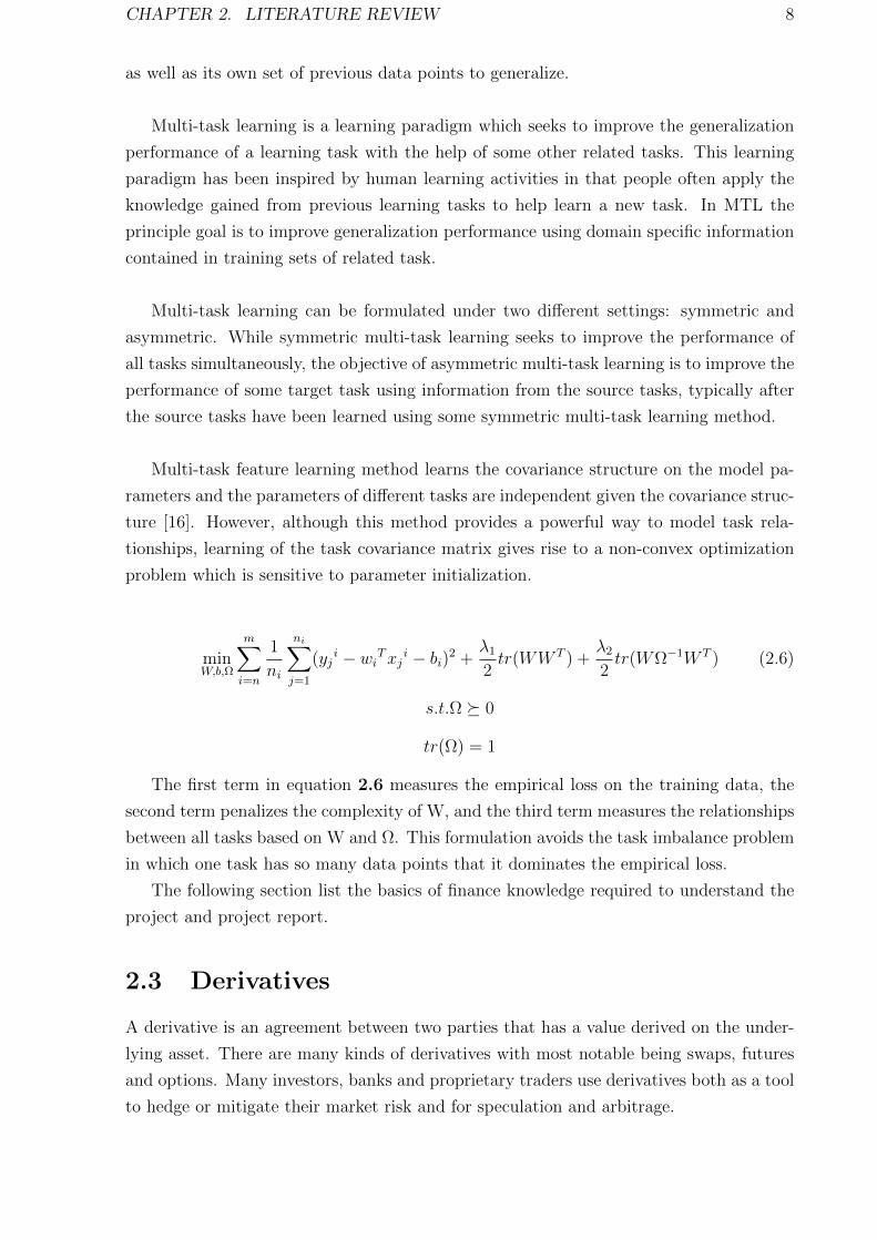
minW,b,Ω

m∑i=n

1

ni

ni∑j=1

(yji − wiTxj i − bi)2 +

λ1

2tr(WW T ) +

λ2

2tr(WΩ−1W T ) (2.6)

s.t.Ω 0

tr(Ω) = 1

The first term in equation 2.6 measures the empirical loss on the training data, the

second term penalizes the complexity of W, and the third term measures the relationships

between all tasks based on W and Ω. This formulation avoids the task imbalance problem

in which one task has so many data points that it dominates the empirical loss.

The following section list the basics of finance knowledge required to understand the

project and project report.

2.3 Derivatives

A derivative is an agreement between two parties that has a value derived on the under-

lying asset. There are many kinds of derivatives with most notable being swaps, futures

and options. Many investors, banks and proprietary traders use derivatives both as a tool

to hedge or mitigate their market risk and for speculation and arbitrage.


Common Types of derivative contracts

Futures: A financial contract obligating the buyer to purchase an asset (or the

seller to sell an asset), such as a physical commodity or a financial instrument, at a

predetermined future date and price. The futures markets are characterized by the

ability to use very high leverage relative to stock markets[10]

Options: A financial derivative that represents contract sold by one party (option

writer) to another party (option holder). The contract offers the buyer the right,

but not the obligation, to buy (call) or sell (put) a security or other financial asset

at an agreed-upon price (the strike price) during a certain period of time or on a

specific date (exercise date)[10]

The pay-off for a European call option is given by:

Ct = max(0,St −K) (2.7)

where,

Ct: option price at time t

St: stock price at time t

K: strike price.

Figure 2.2: Call option pay-off diagram

The option price can be broken down into two components:

a. Intrinsic Value

b. Time Value

Option Value = Intrinsic Value + Time Value

Intrinsic Value is fairly straight forward to calculate. However, to model the Time Value

of the option is the main challenge.


Futures and Options are widely used by investors and traders to leverage their

investments to gain multiple returns and/or manage their risk exposure. In Indian

markets National Stock exchange (NSE) and Bombay Stock exchanges (BSE) are the

two major exchanges. The graph below shows the contribution of futures and options in

derivative trading on NSE. With increasing popularity of Options over the years in

financial markets, pricing it correctly becomes important.

Chapter 3

Methodology

3.1 Methods

Despite SVR and HKL being powerful non-parametric data driven approach for option

pricing, very few have actually used these methods for financial econometric applications.

The parametric models are highly suited for developed and highly liquid market but not

in general for emerging markets like India. Model capacity for SVR & HKL models is

part of the optimization problem but cross-validation is needed to properly select the

model parameters, to fine tune them and adapt them to the sample data for ensuring

high out-of-sample accuracy.

SV regression, HKL and MTL have already been described in brief in chapter 2. In this

chapter we look at different kernels used for these methods. This section also provides

a description of Auto-Regressive Integrated Moving Average (ARIMA) and clustering

methods. Various hybrid models have been built using the above mentioned methods and

their performances are tabulated in the chapter 4

3.1.1 SV regression: Radial Basis function (RBF) kernel

RBF kernel non-linearly maps samples into a higher dimensional space unlike linear ker-

nels. Linear kernel is a special case of RBF (Keerti and Lin, 2003), since the linear kernel

with a penalty parameter C has the same performance as the RBF kernel with some pa-

rameter (C, γ). The libsvm library reported in [8] is used for the purpose of experiments.

RBFkernel : K(xi,xj) = exp(−γ||xi − xj||2), γ > 0 (3.1)

11

CHAPTER 3. METHODOLOGY 12

3.1.2 HKL: Polynomial Kernel

Consider Xi = R, kij(xi, xi′) =

(qj

)(xixi

′)j; the full kernel is then equal to k(x, x′) =∏i=1

p(1 + xixi′)q. This is a polynomial kernel which considers polynomial of maximal

degree q.

3.1.3 HKL: ANOVA Kernel

The HKL method selects relevant subsets from the power set (i.e. the set of subsets)

for the Gaussian kernels. The decomposition of ANOVA kernel is exponential but the

methods provided in [6] limits the number of active kernels and selects the relevant subset

in polynomial time.

3.1.4 ARIMA

Due to infrequent trading of the constituent stocks the index exhibit positive autocor-

relation. We can cross-check this using the Durbin-Watson method to test for serial

correlation. Following a model of infrequent trading, the European options on index are

modeled as ARIMA process.

ARIMA stands for Auto-Regressive Integrated Moving Average. Lags of the differenced

series appearing in the forecasting equation are called “auto-regressive” terms, lags of the

forecast errors are called “moving average” terms, and a time series which needs to be

differenced to be made stationary is said to be an “integrated” version of a stationary

series. Random-walk and random-trend models, autoregressive models, and exponential

smoothing models (i.e., exponential weighted moving averages) are all special cases of

ARIMA models [2].

A non-seasonal ARIMA model is classified as an ”ARIMA (p, d, q)” model, where:

p is the number of autoregressive terms,

d d is the number of non-seasonal differences, and

q is the number of lagged forecast errors in the prediction equation

Following the model of infrequent trading the underlying index dynamics are modeled

as an ARIMA process, for pricing European options on index. The input parameters

Nifty series (S), Futures series (F) and implied Volatility series (σimplied) are forecasted

using ARIMA model and then they are fed as in input to the SVR model. For forecasting

the input series is decomposed into trend, seasonality and irregularity. Each of these


decomposed series is forecasted separately, using different experts and then combined

using dynamic topK median methods, wherein the median of the top K best forecasted

series are chosen. We used 86 experts for trend, 33 experts for seasonality and 33 experts

for irregularity [9].

3.1.5 Clustering

Expectation Maximization (EM)

In statistics, an expectation-maximization (EM) algorithm is an efficient iterative proce-

dure to compute the Maximum Likelihood (ML) estimates in the presence of missing or

hidden data. In ML estimation, aim is to estimate the model parameters for which the

observed data are the most likely.

Each iteration of the EM algorithm consists of two processes: The E-step, and the

M-step. In the expectation, or E-step, the missing data are estimated given the observed

data and current estimate of the model parameters. This is achieved using the conditional

expectation, explaining the choice of terminology. In the M-step, the likelihood function

is maximized under the assumption that the missing data are known. The estimate of

the missing data from the E-step is used in lieu of the actual missing data. Convergence

is assured since the algorithm is guaranteed to increase the likelihood at each iteration

K-Means

K-means method will produce exactly k different clusters of greatest possible distinction.

We start with k random clusters, and then move objects between those clusters with the

goal to:

a. minimize variability within clusters and

b. maximize variability between clusters

In both, k-means & EM methods the number of clusters in data are not known proiri,

and in fact no definite answer can be given what value k should take. This has to be

determined by cross-validation.

MyAlgo

Due to parameter instability the exact relationship between the input data and output

(option price) can’t be estimated properly. The clustering technique described here is not

computationally demanding and is based on conjunction of two fairly simple and straight

forward criteria: moneyness ratio (S/K) and time to maturity (T).


a. DITM

Cluster-1 if (S/K < 0.85 & T < 7)

Cluster-2 if ((S/K < 0.85 & T > 7)

b. ITM

Cluster-1 if (0.85 ≤ S/K < 0.95 & T < 7)

Cluster-2 if (0.85 ≤ S/K < 0.95 & T > 7)

c. ATM

Cluster-1 if (0.95 ≤ S/K < 1.05 & T <7)

Cluster-2 if (0.95 ≤ S/K < 1.05 & T > 7)

d. OTM

Cluster-1 if (1.05 ≤ S/K < 1.15 & T>7)

Cluster-2 if (1.05 ≤ S/K <1.05 & T < 7)

e. DOTM

Cluster-1 if (1.15 ≤ S/K & T < 7)

Cluster-2 if (1.15 ≤ S/K & T > 7)

3.2 Models

In this study, the main focus is on exploring non-parametric models as a pricing tool for

European options in context with Indian markets and to compare them with parametric

OPMs. The main aim is application of machine learning techniques to Option Pricing

scenario. Different hybrid models are built using these methods.

The models can be broadly classified into:

a. Black-Scholes model (parametric)

b. SVM model

c. HKL models with polynomial & ANOVA kernels

d. MTL model

e. Hybrid model (Clustering & SVM) and

f. Hybrid model (forecasted inputs & SVM)

Table 3.1 lists the different models and their brief description.


The SV regression is performed using RBF kernel described in section 3.1.1. SVR

model estimates option price for different input parameters. The model approximates the

unknown empirical options pricing function explicitly by modeling the market prices of

the call options. The combination of model parameters for which the mean-squared error

for 4-fold cross validation came out to be minimum, was chosen. The inputs are scaled in

range from [0, 1] for the purpose of support vector regression.

The Black-Scholes model described in section 2.1.1 uses Spot Nifty price (S), Strike

price (K), Volatility (σ), Time to maturity (T) and Risk-free rate (r) as inputs. In ad-

dition to the standard Black-Scholes parameters more input parameters are added to

the model based on squared correlation coefficient R2. The new parameters include im-

plied volatility (σimplied), Futures series (F), number of contracts (η), Gold price (G) and

Crude oil price (Coil). σimplied is calculated using Black-Scholes equation. Commodities

such as Gold and Crude Oil fall in different asset class providing diversification benifits

to an investor compared to Equities. They have significant correlation with the market

indices.The futures series and implied volitility have greater contribution to explain the

behavior of the option series. The number of contarcts traded represents the liquidity of

an option.

MTL method described in section 2.2.3 is used for exploring relation between related

tasks (S, F, σimplied & option price). A hybrid model is built using MTL method which

is used to model the input parameters and then the predicted values are fed to the SV

Regression model.

To the knowledge none of the studies used such a broad set of input parameters for the

option pricing. The results have shown, including these set of parameters improves the

pricing performance of the model. Option pricing in context of Indian markets has not

been explored yet. One can’t predict accurately the market sentiment and investor be-

havior but using these additional set of input parameters aid in modeling the information

contained in their current market prices.

3.3 Cross-Validation

Each of the model is cross-validated for selecting best model parameters. SVM, HKL and

MTL are all adapted to output the best possible combination of model parameter for the

training data. Using these parameters the model is built which is then used to forecast

out-of-sample data. In each of these methods parameters are estimated using a grid-search

method. For each parameter setting cross-validation (CV) accuracy is measured in terms

of mean square error (MSE).


3.4 Data Filtering

Based on empirical data it is reasonable to assume that in a given month Nifty index

movement is not more than 5% on either side. For the purpose of this study the options

data is classified into five series: deep in-the-money (DITM), in-the-money (ITM), at-

the-money (ATM), out-of-money (OTM) and deep out-of-money (DOTM), depending on

the difference between the index price(S) and strike price(K). Few of the parameters are

processed and not used in their available form (e.g. Moneyness ratio & intrinsic value)

were used instead of Strike Price (K).


ModelName

Methods Description

Parametricmodel

BSBlack-Scholesequation

This is the benchmark Black-Scholes model. Perfor-mance of other models is compared against this para-metric option pricing model. Inputs to this model is Spotprice of Nifty(S), annualized historical volatility(σ), Timeto maturity(T) and Strike price(K).

SupportVectorMachine(SVM)

SVM-BS

RBF ker-nel

A similar model was developed by [4], The model uses thestandard BS parameters as input. The kernel functionused is RBF. Model parameters were selected after cross-validation using grid search approach

SVM-new

RBF ker-nel

In addition to the BS parameters, new parameters areadded which served as an input to the model. The pa-rameters were selected by considering the squared corre-lation coefficient R2

HierarchicalKernelLearning(HKL)

HKL-poly

Polynomialkernel

This method uses polynomial kernel described in section3.1.2 as a kernel for HKL method. The number of activekernel is determined by the algorithm described in [6]

HKL-ANOVA

ANOVAkernel

This method uses ANOVA kernel described in section3.1.3 as a kernel for HKL method. The number of activekernel is determined by the algo described in section [6]

ClusteringHybridmodel

EMEM algo& SVR

This is a hybrid model uses EM algorithm described insection 3.1.5 to cluster the series into two cluster basedon moneyness ratio(S/K) & time to maturity(T). SV re-gression is then applied to each of these clusters sepa-rately to determine best model parameters.

KMK-meansalgo &SVR

This is a hybrid model uses K-means algorithm describedin section 3.1.5 to cluster the series into two cluster basedon moneyness ratio(S/K) & time to maturity(T). SV re-gression is then applied to each of these clusters sepa-rately to determine best model parameters.

MyAlgo S/K & TIn this method the clustering is done on the basis of sim-ple logical conditions based on moneyness ratio & timeto maturity

ForecastinputparametersHybridmodel

MTL-SVM

MTL& RBFkernel

This model uses MTL method described in [16]. Theinput parameters(S, F, implied volatility) are forecastedsimultaneously and then fed to the SV regression modelto get the best model parameters

ARIMA-SVM

ARIMA& RBFkernel

The model first decomposes the series(S, F & σimplied)into trend, seonality & irregularity component and arethen forecasted independently. Each of these is then com-bined using dynamic topK median values. The output ofthese series is then fed to SV regression model to get thebest model parameters.

Multi-TaskLearning

MTL MTLIn this method a set of similar task(S, F, σimplied & C) isfed to the MTL model. The MTL method learns simul-teneously all the task and is used for prediction

Table 3.1: Model description table

Chapter 4

Data and Results

4.1 Data

The analysis used data on S&P CNX Nifty index call options traded on National Stock Ex-

change (NSE) over the period from January 2008 to July 2010 with 21372 data points.

The options with 1-month to expiry are considered for the purpose of this study. Most

of the option pricing studies have been done on the US market data. Emerging market

inherently beahve differntly compared to the developed markets like the US. India being

one of the most popular emerging markets, the S&P Nifty Index call options are consid-

ered for the purpose of this study. Out of the entire index options traded on (NSE) Nifty

index option accounts for 99.95% of the total traded volume with an average monthly

turnover of over Rs. 6.7 trillion. The daily closing values of the Nifty index call options

were taken from NSE’s archive section [1]. The 3-month MIBOR (Mumbai interbank offer

rate) rates are used instead of the standard risk-free government bond rates, to account

for the real risk-free market rates.

Based on empirical data it is reasonable to assume that in a given month Nifty index

moment is not more than 5% on either side. For the purpose of this study the options

data is classified into five series depending on the difference between the index price and

strike price. The dataset was then scaled in between [0, 1]. The data points with 0 days

to maturity were removed from the sample data.

i. deep in-the-money (DITM)

ii. in-the-money (ITM)

iii. at-the-money (ATM)

iv. out-of-money (OTM)

v. deep out-of-money (DOTM)

18

CHAPTER 4. DATA AND RESULTS 19

4.2 Performance measurement

The pricing performance of different models are quantified based on some error measure-

ment parameters. In most of the studies mean squared error is used as a performance

measurement criteria and is more intutive.

4.2.1 Mean Squared Error (MSE)

The mean squared error of an estimator is one of the ways to quantify the difference

between an estimator and the true value of the quantity being estimated.

MSE =1

N

N∑j=0

(observationj − predictionj)2 (4.1)

4.2.2 Explained Variance

In statistics explained variance measures the proportion to which a mathematical model

accounts for variation i.e. apparent randomness of a given data set.

Explained V ariance = 1−σ2predicted values

σ2true values

(4.2)

4.3 Results

In most of the option pricing literature Black-Scholes model is used as the benchmark

model. The results obtained by the different models are compared with the standard

Black-Scholes model. Higher the explained variance value better is the model. Tables

4.1, 4.4 & 4.5 lists 1-day forecast performance of different approaches described in sec-

tion 3.2 compared to the benchmark Black-Scholes model.

For more details refer to the table in Appendix A.1 which lists the Mean Square Error

(MSE) values of the different models for 1-day price forecast of options. Black-Scholes

model prices those options more accurately for which the volatility of the option series is

less. Its evident from the results that proposed models improved performance of pricing

ITM options compared to Black-Scholes. Table A.3 reports the explained variance of dif-

ferent models. High values of explained variance implies the model under consideration

performs well for the problem under consideration.

4.3.1 Feature selection & Improvements

A set of new features were added in addition to the standard Black-Scholes parameters.

The table 4.1 shows the performance of SVM-BS model Vs SVM model. Addition


of new set of features improved the pricing performance of the model drastically across

all the series. Each of the new input parameters helped in modeling the information

contained in market for pricing the options more correctly.

DITM ITM ATM OTM DOTM

SVM-BS 24.6% 8.6% 25.5% 3% 6.4%SVM-new 43.1% 21.1% 51.9% 27.2% 35%

Table 4.1: Model Comparision: 1-day MSE Feature & Improvements

Tables 4.2 and 4.3 lists the performance for HKL & MTL methods compared to the

SVM model built using the additional set of features. The figues for MTL model perfor-

mance suggests that MTL method is able to capture the relationship between different

series quite effectively.


SVM-new 43.1% 21.1% 51.9% 27.2% 35%HKL-poly 41% 22.3% 34.7% 28% 26.1%

HKL-ANOVA 47.2% 38.5% 41.8% 34% 40%

Table 4.2: Model Comparision: HKL Vs SVM


SVM-new 43.1% 21.1% 51.9% 27.2% 35%MTL 39.1% 20.2% 59.7% 41% 58%

Table 4.3: Model Comparision: 1-day MSE Feature & Improvements

4.3.2 Clustering & Improvements

Financial time series often suffer from parameter insatbility i.e. the relation between the

parameters may not be valid when we move from one time hirizon to other. Hybrid models

built using clustering methods and SVM method improved the Option Pricing accuracy.

All the three clustering methods showed improvement in forecast accuracy. The table

4.4 shows relative performance of the clustering methods compared to our benchmark

Black-Scholes model. If we compare the three hybrid models built using clutering tech-

nique and the pure SVM model, all the tree methods give sizeable improvement. The EM

algorithm performs best across different series. For pricing At-the-money options, which

have high trading volume (i.e. greater liquidity), k-means algorithm for clustering is more

suited. Its evident from the graph that new suggested algoritm for clustering the series

shows comparable performance to k-means algorithm.



SVM-new 43.1% 21.1% 51.9% 27.2% 35%EM 58.4% 49.6% 63.5% 51% 58.8%KM 56.9% 46.4% 73.4% 47.8% 53.5%

MyAlgo 56.7% 43.2% 72.2% 49.6% 58%

Table 4.4: Model Comparision: 1-day MSE Clustering & Improvements

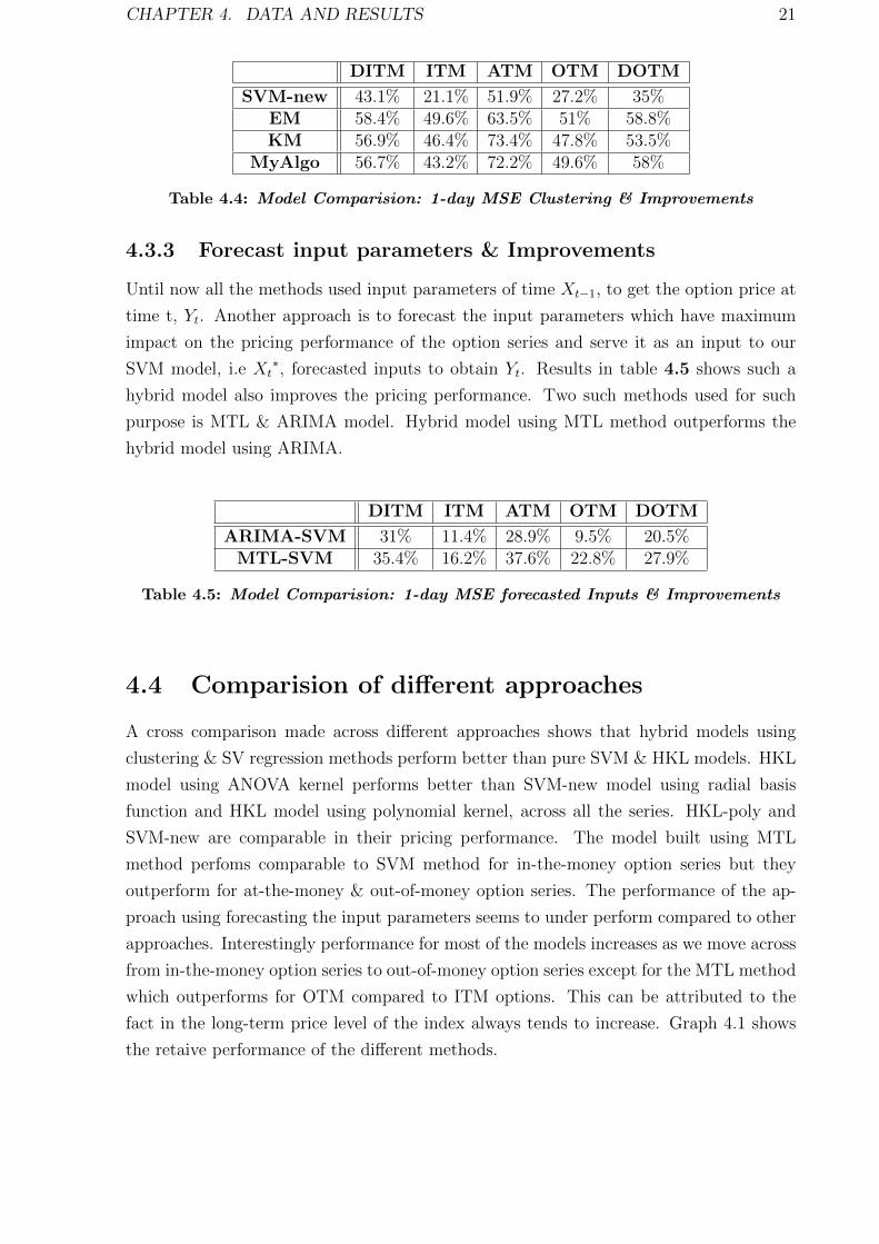
4.3.3 Forecast input parameters & Improvements

Until now all the methods used input parameters of time Xt−1, to get the option price at

time t, Yt. Another approach is to forecast the input parameters which have maximum

impact on the pricing performance of the option series and serve it as an input to our

SVM model, i.e Xt∗, forecasted inputs to obtain Yt. Results in table 4.5 shows such a

hybrid model also improves the pricing performance. Two such methods used for such

purpose is MTL & ARIMA model. Hybrid model using MTL method outperforms the

hybrid model using ARIMA.


ARIMA-SVM 31% 11.4% 28.9% 9.5% 20.5%MTL-SVM 35.4% 16.2% 37.6% 22.8% 27.9%

Table 4.5: Model Comparision: 1-day MSE forecasted Inputs & Improvements

4.4 Comparision of different approaches

A cross comparison made across different approaches shows that hybrid models using

clustering & SV regression methods perform better than pure SVM & HKL models. HKL

model using ANOVA kernel performs better than SVM-new model using radial basis

function and HKL model using polynomial kernel, across all the series. HKL-poly and

SVM-new are comparable in their pricing performance. The model built using MTL

method perfoms comparable to SVM method for in-the-money option series but they

outperform for at-the-money & out-of-money option series. The performance of the ap-

proach using forecasting the input parameters seems to under perform compared to other

approaches. Interestingly performance for most of the models increases as we move across

from in-the-money option series to out-of-money option series except for the MTL method

which outperforms for OTM compared to ITM options. This can be attributed to the

fact in the long-term price level of the index always tends to increase. Graph 4.1 shows

the retaive performance of the different methods.


Figure 4.1: 1-day MSE comparision between differnt approaches

4.5 Comparision: 1-week predictive power of models

Until now we have seen comparision of performance of various model for 1-day price

forecast. In this section we cross-compare between the forecasting power of SVM-new &

MTL model. Table 4.6 reports the values for 1-week price forecast of these models. From

the results its evident that MTL model outperforms SVM in longterm forecasting power.


SVM-longterm 3,824.91 4,865.07 3,223.89 3,003.67 3,710.18SVM-1day 2,786.44 3,084.71 2,548.95 2,579.20 2,406.09

MTL-longterm 3,550.68 4,486.50 2,627.39 2,354.32 2,100.91MTL-1day 2,982.37 3,121.44 2,139.12 2,087.59 1,552.46

Table 4.6: Comparision: Predictive power of models

4.6 Computation Time

In the previous section we described the pricing performance of different model. In this

section we describe the relative computation time requirement of the different methods.

The parametric Black-Scholes method has a closed form solution and is computationally

less demanding compared to other methods. MTL & ARIMA methods with decomposition

require huge amout of time for computation. HKL methods using both polynomial kernel

and ANOVA kernel takes more time to compute than SVM using radial basis function.

Thus in a real-life situation one has to always trade-off between the pricing accuracy and

computation time requirements.


Figure 4.2: Comparision: Predictive power of models

Chapter 5

Conclusion & Future Work

5.1 Conclusion

We investigated the pricing performance of non-parametric machine learning techniques

such as SV Regression (SVR), HKL and MTL methods for Nifty index call options and

compared it with parametric Black-Scholes model for 1-day & 1-week price forecast. Non-

parametric machine learning techniques adjust more rapidly to changing market behavior

and are able to capture the pattern more effectively compared to parametric models. Fi-

nancial data often shows parameter instability and clustering techniques help greatly in

overcoming this pitfall. Multi-Task Learning mmodel & hybrid models built using cluster-

ing techniques improved pricing accuracy over 50% compared to the Black-Scholes model.

The results suggest non-parametric machine learning techniques outperform parametric

Black-Scholes model and are promising enough for problem under consideration. Using

much sophisticated techniques for calibrating the models and filtering the data, pricing

performance can further be improved.

5.2 Future Work

Pricing options is a challenging problem because financial time series are greatly influ-

enced by international, economical and political events.. Current work uses SVR and

Black Scholes model for pricing European call options. These methods can be extended

further to price European Put options. Also, these models are flexible enough to incor-

porate pricing of American Call and Put options.

Derivatives are very useful in trading and hedging in financial markets. Market partici-

pants use options to manage their risk exposure to different asset classes i.e. commodities,

real estates, swaps, mortgages etc. Various complex trading strategies are built using fu-

tures and options for profit maximization. Complex portfolios are built and traded in

24

CHAPTER 5. CONCLUSION & FUTURE WORK 25

the markets, using synthetic and highly sophisticated derivative products. Portfolio op-

timization and trading is an extension to the option pricing problem, wherein given a set

of market information and risk preference of an investor, we need to price the portfolio to

maximize returns.

Appendix A

Performance Measurement

A.1 Mean Square Error (MSE)


BS 4,900.53 3,909.32 5,304.43 3,540.57 3,700.21SVM-BS 3,693.43 3,573.20 3,953.12 3,433.39 3,462.06SVM-new 2,786.44 3,084.71 2,548.95 2,579.20 2,406.09HKL-poly 2,889.08 3,035.67 3,462.01 2,550.69 2,734.99

HKL-ANOVA 2,589.82 2,404.71 3,087.83 2,335.09 2,221.25MTL 2,982.37 3,121.44 2,139.12 2,087.59 1,552.46EM 2,037.11 1,970.19 1,938.67 1,734.54 1,525.65KM 2,112.32 2,094.17 1,412.06 1,849.16 1,719.94

MyAlgo 2,119.89 2,221.25 1,476.94 1,783.12 1,555.08ARIMA-SVM 3,383.06 3,462.16 3,769.87 3,204.23 2,940.37

MTL-SVM 3,165.62 3,277.84 3,307.72 2,734.99 2,669.23

Table A.1: 1-day Mean Square Error(MSE)

A.2 Percentage improvements over Black-Scholes model

A.3 Model Comparision

Graph A.4 shows the behavior of different option series ITM, ATM & OTM compared

to index Nifty series. The variation in the pattern of the series is due to two factors the

Intrinsic Value & the Time Value of the optins.

A.4 Explained Variance

26

APPENDIX A. PERFORMANCE MEASUREMENT 27


SVM-BS 24.6% 8.6% 25.5% 3% 6.4%SVM-new 43.1% 21.1% 51.9% 27.2% 35%HKL-poly 41% 22.3% 34.7% 28% 26.1%

HKL-ANOVA 47.2% 38.5% 41.8% 34% 40%MTL 39.1% 20.2% 59.7% 41% 58%EM 58.4% 49.6% 63.5% 51% 58.8%KM 56.9% 46.4% 73.4% 47.8% 53.5%

MyAlgo 56.7% 43.2% 72.2% 49.6% 58%ARIMA-SVM 31% 11.4% 28.9% 9.5% 20.5%

MTL-SVM 35.4% 16.2% 37.6% 22.8% 27.9%

Table A.2: Model Comparision: 1-day MSE

Figure A.1: Feature selection & Improvement: 1-day MSE

Figure A.2: Clustering & Improvements: 1-day MSE

APPENDIX A. PERFORMANCE MEASUREMENT 28

Figure A.3: Forecast input parameters & Improvements: 1-day MSE

Figure A.4: Behavior of different series


BS 71.1% 75.2% 46.8% 53.7% 16.3%SVM-BS 78.2% 77.3% 60.3% 55.1% 21.7%SVM-new 83.6% 80.4% 74.4% 66.3% 45.6%HKL-poly 83% 80.7% 65.2% 66.7% 38.2%

HKL-ANOVA 84.7% 84.7% 69% 69.5% 49.8%MTL 82.4% 80.2% 78.5% 72.7% 64.9%EM 88% 87.5% 80.5% 77.3% 65.5%KM 87.5% 86.7% 85.8% 75.8% 61.1%

MyAlgo 87.5% 85.9% 85.2% 76.7% 64.8%ARIMA-SVM 80% 78% 62.2% 58.1% 33.5%

MTL-SVM 81.3% 79.2% 66.8% 64.3% 39.6%

Table A.3: Explained Variance: 1-day forecast models

Bibliography

[1] National stock exchange of india ltd. http://www.nseindia.com/. Accessed: July

2010.

[2] Statistical analysis software, data mining, predictive analysis, credit scoring. http:

//www.statsoft.com/textbook/time-series-analysis/. Accessed: August 2010.

[3] Panayiotis C. Andreou, Chris Charalambous, and Spiros H. Martzoukos. Pricing

and trading european options by combining artificial neural networks and parametric

models with implied parameters. European Journal of Operational Research, 2008.

[4] Panayiotis C. Andreou, Chris Charalambous, and Spiros H. Martzoukos. European

option pricing by using the support vector regression approach. C. Alippi et al.

(Eds.): ICANN, 2009.

[5] Panayiotis Ch. Andreou, Chris Charalambous, and Spiros H. Martzoukos. Critical

assessment of option pricing methods using artificial neural networks. Springer-Verlag

Berlin Heidelberg, 2002.

[6] F. Bach. Exploring large feature spaces with hierarchical multiple kernel learning.

In Advances in Neural Information Processing Systems (NIPS), 2008.

[7] A. CARELLI, S. SILANI, and F. STELLA. Profiling neural networks for option

pricing. International Journal of Theoretical and Applied Finance, 2000.

[8] Chih-Chung Chang and Chih-Jen Lin. LIBSVM: A library for support vector ma-

chines. ACM Transactions on Intelligent Systems and Technology, 2:27:1–27:27, 2011.

[9] Amit Gupta and Prof. Bernard Menezes. Clustering and forecasting of time series

using global properties. Master’s thesis, Indian Institue of Technology, Bombay, 2010.

[10] John C. Hull. Introduction To Futures And Options Markets. Phi Learning Pvt Ltd,

2009.

[11] PAUL R. LAJBCYGIER and JEROME T. CONNOR. Improved option pricing using

artificial neural networks and bootstrap methods. International Journal of Neural

Systems, 8(4), 1997.

29

http://www.nseindia.com/

http://www.statsoft.com/textbook/time-series-analysis/

http://www.statsoft.com/textbook/time-series-analysis/

BIBLIOGRAPHY 30

[12] Zeynep ltuzer Samur and Gul Tekin Temur. The use of artificial neural network

in option pricing: The case of s&p 100 index options. World Academy of Science,

Engineering and Technology, 2009.

[13] Pawel Radzikowski. Non-parametric methods of option pricing. INFORMS & KO-

RMS, 2000.

[14] M Rubinstein. Implied binomial trees. The Journal of Finance, 49, 1994.

[15] A. J. Smola and B. Scholkopf. A tutorial on support vector regression. Statistics and

Computing, 2003. in press.

[16] Yu Zhang and Dit-Yan Yeung. A convex formulation for learning task relationships in

multi-task learning. Proceedings of the 26th Conference on Uncertainty in Artificial

Intelligence (UAI), pages 733–742, 2010.

Option Pricing using Machine Learning techniquessaketh/research/DeodaDDP.pdf · Option Pricing...

Documents

Transcript of Option Pricing using Machine Learning techniquessaketh/research/DeodaDDP.pdf · Option Pricing...