CEFIN – Centro Studi di Banca e Finanza Dipartimento di Economia Aziendale – Università di Modena e Reggio Emilia

Viale Jacopo Berengario 51, 41100 MODENA (Italy) tel. 39-059.2056711 (Centralino) fax 059 205 6927

CEFIN Working Papers No 11

Option based forecasts of volatility: An empirical study in the DAX index options market

by Silvia Muzzioli

May 2008

1

Option based forecasts of volatility:

An empirical study in the DAX index options market

S. Muzzioli1*

Abstract

Option based volatility forecasts can be divided into “model dependent” forecast, such as

implied volatility, that is obtained by inverting the Black and Scholes formula, and “model free”

forecasts, such as model free volatility, proposed by Britten-Jones and Neuberger (2000), that do

not rely on a particular option pricing model.

The aim of this paper is to investigate the unbiasedness and efficiency in predicting future

realized volatility of the two option based volatility forecasts: implied volatility and model free

volatility. The comparison is pursued by using intradaily data on the Dax-index options market. Our

results suggest that Black-Scholes volatility subsumes all the information contained in historical

volatility and is a better predictor than model free volatility.

Keywords: Implied Volatility, Model free volatility, Volatility Forecasting.

JEL classification: G13, G14.

1 Department of Economics and CEFIN, University of Modena and Reggio Emilia, Viale Berengario 51, 41100

Modena (I), Tel. +390592056771 Fax +390592056947, e-mail: silvia.muzzioli@unimore.it

* The author wishes to thank Giuseppe Marotta for helpful comments and suggestions The author gratefully acknowledges financial support from MIUR. Usual disclaimer applies.

2

1. Introduction

Volatility estimation and forecasting are essential both for the pricing and the risk

management of derivative securities. There have been various contributions aimed at assessing the

best way in order to forecast volatility. Among the various models proposed in the literature we

distinguish between option based volatility forecasts that use prices of traded options in order to

unlock volatility expectations and time series volatility models that use historical information in

order to predict future volatility.

Following Poon and Granger (2003), among time series volatility models, we have

predictions based on past standard deviation, ARCH conditional volatility models and stochastic

volatility models. Among prediction based on past standard deviation we have the simple random

walk hypothesis in which the best estimate of future realised volatility is today volatility, methods

based on averages, such as historical averages, moving averages and exponential smoothing moving

averages, that try to solve the trade off between having as much observations as possible and

sampling close to the present time and simple regression models that regress volatility on its past

values. ARCH family conditional volatility models (see Bollerslev, Chou and Kroner (1992) for a

survey) formulate conditional variance as a function of past squared returns via maximum

likelihood. ARCH models have the advantage that the next step forecast is available by their very

same construction. In Stochastic volatility models (see Ghysels, Harvey and Renault (1996) for a

survey) volatility is driven by a different source of uncertainty from the one of the underlying asset

price. Stochastic volatility models are very flexible, but difficult to implement, since they usually

have no closed form solution.

Among option based volatility forecasts we have implied volatility, that is a “model

dependent” forecast since it relies on the Black and Scholes model, and the so called “model free”

volatility, proposed by Britten-Jones and Neuberger (2000), that does not rely on a particular option

pricing model.

Implied volatility is usually extracted from a single option, by inverting the Black and

Scholes formula, by means of a numerical method such as the bisection method.

Model free Implied Volatility, proposed by Britten-Jones and Neuberger (2000), is based on

the observation that the expected sum of squared returns between two dates is completely specified

by two sets of options expiring on the two dates. Model free implied volatility is derived by using a

cross section of option prices differing in time to maturity, strike prices and option type. Therefore

it should be more informative than implied volatility backed out from a single option. Moreover,

while the examination of the forecasting power of the Black and Scholes implied volatility is a joint

3

test of model specification and market efficiency, model free implied volatility, being independent

from a particular option pricing model, provides a direct test of market efficiency.

The CBOE VIX volatility index is an example of a switch from a Black and Scholes implied

volatility to a model free one (for more details see Carr and Wu (2006)). The CBOE volatility index

expresses a one-month implied volatility and is deemed as a benchmark for stock market volatility

and market fear. Prior to September 2003 it was computed (since then it has been renamed VXO)

by using Black and Scholes implied volatility backed out from eight near to the money options (4

calls and 4 puts) written on the S&P100 at the two nearest maturities. From 22 September 2003, the

CBOE changed the definition and computation rules of the VIX index. The underlying is now the

S&P500 and the computation is based on the model free implied volatility backed out from a cross

section of at and out of the money call and put options for the two nearest maturities.

A drawback of using Black and Scholes implied volatility is clearly its dependence on the

strike price of the option (the so-called smile effect), time to maturity of the option (term structure

of volatility) and option type (call versus put). Many papers have investigated the information

content of implied volatility backed out from different option classes. Christensen and Prabhala

(1998) examine the relation between implied and realized volatility on S&P100 options, on the time

period 1983-1995. They found that at the money calls are good predictors of future realized

volatility. Fleming (1998) investigates the implied-realised volatility relation in the S&P100 options

market and finds that at the money call implied volatility has slightly more predictive power than

put implied volatility. Ederington and Guan (2005) examine how the information in implied

volatility differs by strike price for options on S&P500 futures. They point out that implied

volatilities calculated from moderately high strike options (moderately out of the money calls and in

the money puts) are efficient predictors of future volatility and fully embed all the available

information, while implied volatilities calculated from low strikes (out of the money puts and in the

money calls) and at the money strikes are biased and less efficient predictors of future volatility.

They conclude that the information content in implied volatilities varies roughly in a mirror image

of the implied volatility smile.

Nonetheless, at the money Black and Scholes volatility is usually considered as the market’s

expectation of future realised volatility between now and the expiration date of the option. Even if

from a theoretical point of view there is no clear reason for that, since the Black and Scholes model

postulates a constant volatility, from an empirical point of view, various papers have demonstrated

the soundness of such a choice. In fact, numerous papers have analysed the empirical performance

of at the money Black Scholes implied volatility in various option markets, ranging from indexes,

futures or individual stocks and find that implied volatility is an unbiased and\or efficient forecast

4

of future realised volatility (see e.g. Christensen and Prabhala (1998) for options on indexes,

Ederington and Guan (2002) for options on Futures, Szakmary et al. (2003) and Godbey and Mahar

(2005) for options on individual stocks and Blair, Poon and Taylor (2001b) and Bandi and Perron

(2006) for the VIX volatility index).

Up to now, very few papers have dealt with the forecasting power of model free implied

volatility. From a theoretical point of view, Carr and Wu (2006) highlight that model free volatility

should be superior to Black Scholes volatility. In fact, they showed that at the money Black Scholes

implied volatility can be considered as a proxy of a volatility swap rate, while model free volatility

is a proxy for a variance swap rate. While the payoff on a volatility swap is difficult to replicate, the

payoff of a variance swap rate is easily replicable by using a static position in a continuum of

European options and a dynamic position in futures. From an empirical point of view, the evidence

in favour of the superiority of model free volatility against Black Scholes volatility is mixed. Lynch

and Panigirtzoglou (2003) analyse the predictive power of model free implied volatility on four

different markets: S&P500, FTSE100, Eurodollar and sterling futures and find model free implied

volatility is a biased though efficient estimate of future volatility. Jiang and Tian (2005) investigate

the predictive power of the model free volatility in the S&P500 options. They find that model free

implied volatility is an efficient forecast of future realised volatility and an unbiased forecast after a

constant adjustment and subsumes all the information contained in the Black and Scholes implied

volatility. On the other hand, Andersen and Bondarenko (2007) found opposite results. They

investigate the forecasting performance of model free implied volatility in the S&P 500 futures

market and find that it does not perform better than the simple Black and Scholes volatility.

The aim of this paper is to investigate the unbiasedness and efficiency in predicting future

realized volatility of the two option based volatility forecasts: implied volatility and model free

volatility. In order to pursue a fair comparison with model free implied volatility, that is derived

based on a cross section of option prices, for implied volatility we use a weighted average of

implied volatilities backed out from different option classes. The comparison is performed by using

intradaily data on the Dax-index options market. The market is chosen for two main reasons. First,

the options are European, therefore the estimation of the early exercise premium is not needed and

can not influence the results. Second, the Dax index is a capital weighted performance index

composed of 30 major German stocks and is adjusted for dividends, stocks splits and changes in

capital. Since dividends are assumed to be reinvested into the shares, they do not affect the index

value.

The plan of the paper is the following. In section 2 we illustrate the theoretical concept of

model free implied volatility and we show the practical problems arising in the implementation. In

5

section 3 we present the data set used, the sampling procedure and the variables definitions. In

section 4 we describe the methodology used in order to address the unbiasedness and efficiency of

the different volatility forecasts. In section 5 we report the results of the univariate and

encompassing regressions and we test for robustness our methodology in order to see if some errors

in variables problem may have affected our results. In order to analyze the dependence of model

free volatility on the range of strike price used, in section 6 we present an alternative

implementation of model free volatility. The last section concludes. In Appendix 1 we discuss

some implementation issues for model free volatility.

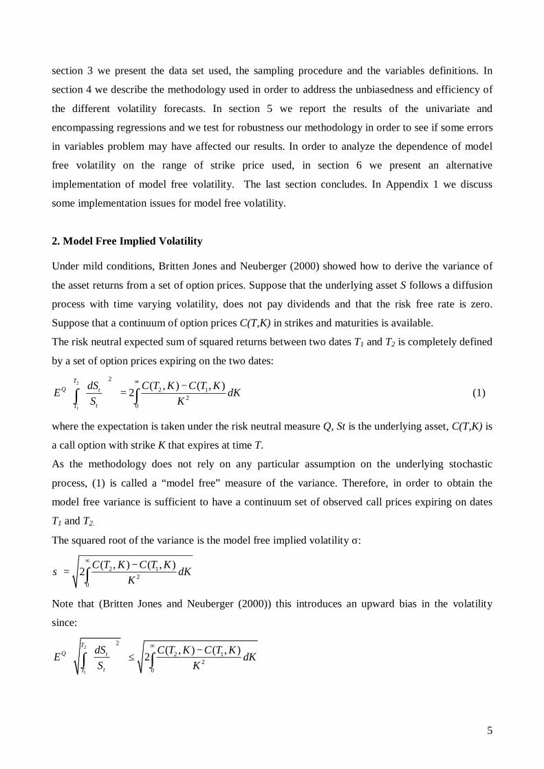
2. Model Free Implied Volatility Under mild conditions, Britten Jones and Neuberger (2000) showed how to derive the variance of

the asset returns from a set of option prices. Suppose that the underlying asset S follows a diffusion

process with time varying volatility, does not pay dividends and that the risk free rate is zero.

Suppose that a continuum of option prices C(T,K) in strikes and maturities is available.

The risk neutral expected sum of squared returns between two dates T1 and T2 is completely defined

by a set of option prices expiring on the two dates:

2

1

2

2 12

0

( , ) ( , )2T

Q t

tT

dS C T K C T KE dKS K

∞ − = ∫ ∫ (1)

where the expectation is taken under the risk neutral measure Q, St is the underlying asset, C(T,K) is

a call option with strike K that expires at time T.

As the methodology does not rely on any particular assumption on the underlying stochastic

process, (1) is called a “model free” measure of the variance. Therefore, in order to obtain the

model free variance is sufficient to have a continuum set of observed call prices expiring on dates

T1 and T2.

The squared root of the variance is the model free implied volatility σ:

2 12

0

( , ) ( , )2 C T K C T K dKK

σ∞ −

= ∫

Note that (Britten Jones and Neuberger (2000)) this introduces an upward bias in the volatility

since:

2

1

2

2 12

0

( , ) ( , )2T

Q t

tT

dS C T K C T KE dKS K

∞ − ≤ ∫ ∫

6

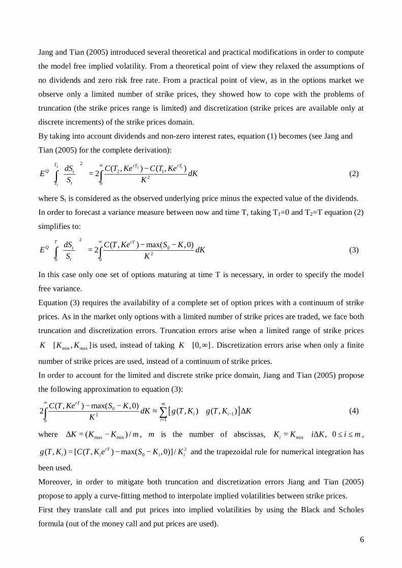
Jang and Tian (2005) introduced several theoretical and practical modifications in order to compute

the model free implied volatility. From a theoretical point of view they relaxed the assumptions of

no dividends and zero risk free rate. From a practical point of view, as in the options market we

observe only a limited number of strike prices, they showed how to cope with the problems of

truncation (the strike prices range is limited) and discretization (strike prices are available only at

discrete increments) of the strike prices domain.

By taking into account dividends and non-zero interest rates, equation (1) becomes (see Jang and

Tian (2005) for the complete derivation):

2 2 1

1

2

2 12

0

( , ) ( , )2T rT rT

Q t

tT

dS C T Ke C T KeE dKS K

∞ − = ∫ ∫ (2)

where St is considered as the observed underlying price minus the expected value of the dividends.

In order to forecast a variance measure between now and time T, taking T1=0 and T2=T equation (2)

simplifies to: 2

02

0 0

( , ) max( ,0)2T rT

Q t

t

dS C T Ke S KE dKS K

∞ − − = ∫ ∫ (3)

In this case only one set of options maturing at time T is necessary, in order to specify the model

free variance.

Equation (3) requires the availability of a complete set of option prices with a continuum of strike

prices. As in the market only options with a limited number of strike prices are traded, we face both

truncation and discretization errors. Truncation errors arise when a limited range of strike prices

min max[ , ]K K K∈ is used, instead of taking [0, ]K ∈ ∞ . Discretization errors arise when only a finite

number of strike prices are used, instead of a continuum of strike prices.

In order to account for the limited and discrete strike price domain, Jiang and Tian (2005) propose

the following approximation to equation (3):

[ ]012

10

( , ) max( ,0)2 ( , ) ( , )rT m

i ii

C T Ke S K dK g T K g T K KK

∞

−=

− −≈ + ∆∑∫ (4)

where max min( ) /K K K m∆ = − , m is the number of abscissas, min ,iK K i K= + ∆ 0 i m≤ ≤ ,

20( , ) [ ( , ) max( ,0)] /rT

i i i ig T K C T K e S K K= − − and the trapezoidal rule for numerical integration has

been used.

Moreover, in order to mitigate both truncation and discretization errors Jiang and Tian (2005)

propose to apply a curve-fitting method to interpolate implied volatilities between strike prices.

First they translate call and put prices into implied volatilities by using the Black and Scholes

formula (out of the money call and put prices are used).

7

Second, they use a curve fitting method (cubic splines), in order to interpolate implied volatilities.

Third, in order to extend the domain of strike prices they suppose that for strikes below the

minimum value the implied volatility is constant and equal to the volatility of Kmin, for strikes

above the maximum value the implied volatility is constant and equal to the volatility of Kmax, i.e

they suppose constant volatility outside the available range of strike prices. It is important to notice

that in this way they are introducing a third source of approximation error that is different from both

truncation and discretization.

Last, they use the Black and Scholes formula in order to convert implied volatilities into call prices,

obtained at the desired strike price frequency.

It is important to remark that the use of the Black and Scholes formula does not affect the model

free attribute of volatility, since it is merely used in order to translate options prices into implied

volatilities.

3. The Data set, the sampling procedure and the variables definitions.

The data set2 consists of intradaily data on DAX-index options, recorded from 1 January

2001 to 31 December 2006. Each record reports the strike price, expiration month, transaction price,

contract size, hour, minute second and centisecond. As for the underlying asset we use intradaily

prices of the DAX-index recorded in the same time period. As a proxy for the risk-free rate we use

the one month Euribor rate.

DAX-options started trading on the German Options and Futures Exchange (EUREX) in

August 1991. They are European options on the DAX-index, which is a capital weighted

performance index composed of 30 major German stocks and is adjusted for dividends, stocks splits

and changes in capital. Since dividends are assumed to be reinvested into the shares, they do not

affect the index value, therefore we do not have to estimate the dividend payments. Moreover the

fact that the options are European avoids the estimation of the early exercise premium. This latter

feature is very important since our data set is by construction less prone to estimation errors if

compared to the majority of previous studies that use American style options. DAX-index options

are quoted in index points, carried out one decimal place. The contract value is EUR 5 per DAX

index point. The tick size is 0.1 of a point representing a value of EUR 0.50. They are cash settled,

payable on the first exchange trading day immediately following the last trading day. The last

trading day is the third Friday of the expiration month, if that is an exchange day, otherwise the

2 The data source for Dax-index options and Dax index is the Institute of Finance, Banking, and Insurance of the University of Karlsruhe (TH), the risk-free rate is available in Data-Stream.

8

exchange trading day immediately prior to that Friday. The final settlement price is the value of the

DAX determined on the basis of the collective prices of the shares contained on the DAX index as

reflected in the intra-day trading auction on the electronic system of the Frankfurt Stock Exchange.

Expiration months are the three near calendar months within the cycle March, June, September and

December as well as the two following months of the cycle June and December.

Several filters are applied to the option data set. First, we eliminate option prices that are

smaller than 1 Euro, since the closeness to the tick size may have affected the true option value.

Second, in order not to use stale quotes, we eliminate options with trading volume less than one

contract. Third, following Jiang and Tian (2005) in order to use only at the money and out of the

money options, we eliminate in the money options (call options with moneyness (X/S) < 0,97 and

put options with moneyness (X/S) > 1,03). Fourth, we eliminate option prices violating the standard

no arbitrage bounds3. Finally, in order to reduce computational burden, we only retain options that

are traded between 2.00 and 3.00 p.m.

As for the sampling procedure, in order to avoid the telescoping problem described in

Christensen, Hansen and Prabhala (2001), we use monthly non-overlapping samples. In particular,

we collect the prices recorded on the Wednesday that immediately follows the expiry of the option

(third Saturday of the expiry month) since the week immediately following the expiration date is

one of the most active. These options have a fixed maturity of almost one month (from 17 to 22

days to expiration). If the Wednesday is not a trading day we move to the trading day immediately

following.

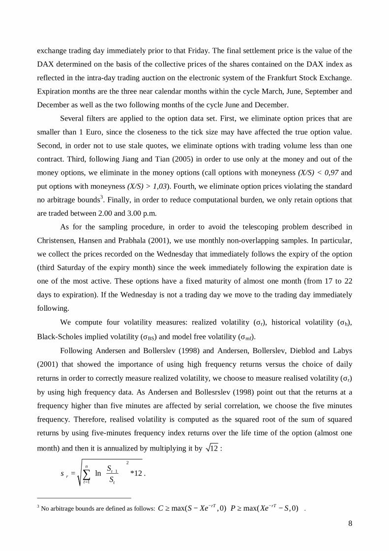
We compute four volatility measures: realized volatility (σr), historical volatility (σh),

Black-Scholes implied volatility (σBS) and model free volatility (σmf).

Following Andersen and Bollerslev (1998) and Andersen, Bollerslev, Dieblod and Labys

(2001) that showed the importance of using high frequency returns versus the choice of daily

returns in order to correctly measure realized volatility, we choose to measure realised volatility (σr)

by using high frequency data. As Andersen and Bollesrslev (1998) point out that the returns at a

frequency higher than five minutes are affected by serial correlation, we choose the five minutes

frequency. Therefore, realised volatility is computed as the squared root of the sum of squared

returns by using five-minutes frequency index returns over the life time of the option (almost one

month) and then it is annualized by multiplying it by 12 :

2

1

1

ln *12n

tr

t t

SS

σ +

=

=

∑ .

3 No arbitrage bounds are defined as follows: max( ,0) max( ,0)rT rTC S Xe P Xe S− −≥ − ≥ − .

9

where n is the number of index prices spaced by five minutes in the one month period.

Historical volatility (σh) is taken as the lagged (one month before) realised volatility.

As for the Model free implied volatility (σmf), the following procedure, based on Jang and

Tian (2005) has been used in order to compute the right hand side of equation (4). We start from the

cleaned data set of option prices that is made of at the money and out of the money call and put

prices recorded from 3.00 to 4.00 p.m. We need a set of option prices with strike prices K ranging

from Kmin to Kmax. As only a limited number of strike prices is available, we need to interpolate

option prices in order to generate the missing prices. Due to the non linear relation between option

prices and strike prices, we follow Shimko (1993) and Ait-Sahalia and Lo (1998) and we perform a

curve-fitting method to interpolate implied volatilities between strike prices, rather than option

prices.

We compute call and put implied volatilities by using synchronous prices, matched in a one minute

interval, by inverting the Black and Scholes formula. As we are using option prices that are traded

in one hour interval, we obtain different implied volatilities for the same strike price, depending on

the time of the trade. Therefore, in order to have a one to one mapping between strikes and implied

volatilities, we group implied volatilities that correspond to the same strike price by computing the

average. In order to have a smooth function, following Bates (1991) and Campa, Chang and Reider

(1998) we use cubic splines to interpolate implied volatilities.

In order to extend the domain of strike prices, following Jiang and Tian (2005) we suppose constant

volatility outside the available range of strikes: for strikes below the minimum value the implied

volatility is equal to the volatility of Kmin, for strikes above the maximum value the implied

volatility is equal to the volatility of Kmax. The domain of strike prices is extended by using a factor

u such that: /(1 ) (1 )S u K S u+ ≤ ≤ + , for the current implementation u has been chosen to be equal

to 0,5. In order to have a sufficient discretization of the integration domain, we compute strikes

spaced by an interval 10K∆ = . In Appendix 1 we discuss some implementation issues on the

truncation (choice of u) and discretization (choice of ∆K) errors of model free volatility, while in

Appendix 2 we analyse the extrapolation errors given by the artificial extension of the strike price

domain outside the existing range by deriving a model free volatility by using only traded option

prices and performing a comparison with the model free volatility obtained following the Jiang ang

Tian extrapolation methodology.

Finally, we use the Black and Scholes formula in order to convert implied volatilities into call

prices. As we need a single value for the underlying asset, we take the average value of the

underlying in the hour of trades.

10

In order to compute the Black and Scholes implied volatility (σBS) we use the following

procedure. First we compute call and put implied volatilities, with the Black and Scholes formula,

for the options closest to being at the money i.e. with strikes one below and one above the

underlying price, by using synchronous prices, matched in a one minute interval. As we are using

option prices that are traded in one hour interval, we compute the average implied volatility for the

two close to the money strike prices. Black and Scholes implied volatility is defined as the weighted

average of the two implied volatilities, with weights inversely proportional to the distance to the

moneyness (for example if the DAX-index is 5355 and the closest strikes are 5400 and 5350 the

implied volatility of the 5400 strike will be weighted 5/50 against the implied volatility 5350 strike

which is weighted 45/50). As we need a single value for the underlying asset, we take the average

value of the underlying in the hour of trades.

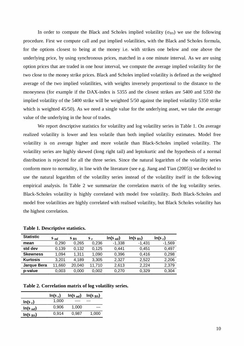
We report descriptive statistics for volatility and log volatility series in Table 1. On average

realized volatility is lower and less volatile than both implied volatility estimates. Model free

volatility is on average higher and more volatile than Black-Scholes implied volatility. The

volatility series are highly skewed (long right tail) and leptokurtic and the hypothesis of a normal

distribution is rejected for all the three series. Since the natural logarithm of the volatility series

conform more to normality, in line with the literature (see e.g. Jiang and Tian (2005)) we decided to

use the natural logarithm of the volatility series instead of the volatility itself in the following

empirical analysis. In Table 2 we summarize the correlation matrix of the log volatility series.

Black-Scholes volatility is highly correlated with model free volatility. Both Black-Scholes and

model free volatilities are highly correlated with realised volatility, but Black Scholes volatility has

the highest correlation.

Table 1. Descriptive statistics.

Statistic σmf σBS σr ln(σmf) ln(σBS) ln(σr) mean 0,290 0,265 0,236 -1,338 -1,431 -1,569 std dev 0,139 0,132 0,125 0,441 0,451 0,497 Skewness 1,094 1,311 1,090 0,396 0,416 0,298 Kurtosis 3,201 4,189 3,305 2,327 2,522 2,206 Jarque Bera 11,660 20,040 11,710 2,613 2,224 2,379 p-value 0,003 0,000 0,002 0,270 0,329 0,304

Table 2. Correlation matrix of log volatility series.

ln(σr) ln(σmf) ln(σBS) ln(σr) 1,000 ---- ---

ln(σmf) 0,906 1,000 ---

ln(σBS) 0,914 0,987 1,000

11

4. The methodology.

The information content of implied volatility is examined both in univariate and in

encompassing regressions. Even if, from a theoretical point of view, it is good practice to start from

the general encompassing regression and analyse in turn the nested regressions, in order to keep the

outline of the analysis consistent with the related literature, we examine first the univariate

regressions and second the more general encompassing regressions.

In univariate regressions, realized volatility is regressed against one of the three volatility

forecasts: Black-Scholes implied volatility (σBS), model free volatility (σmf), or historical volatility

(σh), in order to examine the forecasting ability of each volatility estimator. The univariate

regressions are the following:

ln( ) ln( )r iσ α β σ ε= + + (5)

where σr = realized volatility and σi= volatility forecast, i=h,BS, mf.

In encompassing regressions, realized volatility is regressed against two or more volatility

forecasts in order to distinguish which one has the highest explanatory power and to address

whether a single volatility forecast subsumes all the information contained in the others. Therefore

we first compare pairwise one option based forecast (Black-Scholes implied volatility, model free

volatility) with historical volatility in order to see if one of the option based forecast subsumes all

the information contained in historical volatility. Second we compare the two option based forecast:

Black-Scholes implied volatility and model free volatility, in order to distinguish which one carries

most information on future realised volatility. Third we regress realised volatility on the three

volatility forecasts in order to see the relative importance of each forecast.

The encompassing regressions used are the following:

ln( ) ln( ) ln( )r i hσ α β σ γ σ ε= + + + (6)

where σr = realized volatility, σi= implied volatility, i = BS, mf and σh = historical volatility.

ln( ) ln( ) ln( )r BS mfσ α β σ γ σ ε= + + + (7)

where σr = realized volatility, σBS= Black-Scholes implied volatility and σmf = model free volatility.

ln( ) ln( ) ln( ) ln( )r BS mf hσ α β σ γ σ δ σ ε= + + + + (8)

where σr = realized volatility, σBS= Black-Scholes implied volatility and σmf = model free volatility

and σh = historical volatility.

In univariate regressions (5), we test three hypotheses, following Christensen and Prabhala

(1998). The first hypothesis is H0: 0β = : if the volatility forecast contains some information about

future realised volatility, then the slope coefficient should be different from zero. Therefore we test

if 0β = and we see whether it can be rejected. The second hypothesis is H0: 0=α and 1=β and

12

assesses the unbiasedness of the volatility forecast. If the volatility forecast is an unbiased estimator

of future realised volatility, then the intercept should be zero and the slope coefficient should be

one. In case this latter hypothesis is rejected, we see if at least the slope coefficient is equal to one

(H0: 1=β ) and, if confirmed, we interpret the volatility forecast as unbiased after a constant

adjustment. Finally if implied volatility is efficient then the error term should be white noise and

uncorrelated with the information set.

In encompassing regressions (6) we test two hypotheses. First we test H0: 0=γ i.e. whether

one of the two option based forecasts (Black-Scholes implied, model free volatility) subsumes all

the information contained in historical volatility. Moreover, as a joint test of information content

and efficiency we test in equations (6) if the slope coefficients of historical volatility and one of the

option based forecasts (Black-Scholes implied, model free volatility) are equal to zero and one

respectively (H0: 0=γ and 1=β ). Following Jiang and Tian (2005), we ignore the intercept in the

latter null hypothesis, and if our null hypothesis is verified, we interpret the volatility forecast as

unbiased after a constant adjustment.

In encompassing regressions (7) we investigate the different information content of the two

option based forecasts (Black-Scholes implied, model free volatility). To this end we test, in

regression (7), if 0=γ and 1=β , in order to see if Black-Scholes implied volatility subsumes all

the information contained in model free volatility.

Finally in encompassing regression (8) we investigate the different information content of

the three forecasts (Black-Scholes implied, model free volatility, historical volatility). In order to

assess if the slope coefficient of the Black-Scholes implied volatility subsume all the information

contained in both model free volatility and historical volatility, i.e. the joint hypothesis H0:

0δ = , 0=γ and 1=β .

Christensen and Prabhala (1998) compared the information content of Black and Scholes

implied volatility with historical volatility in the S&P100 index options market. They run both OLS

regressions and EIV regressions in order to correct for potential errors in variables due to the early

exercise feature of the options and the dividend yield estimation and found different results. As our

dataset consists of prices of options on the DAX index that are European style and are written on a

non-dividend paying index, we avoid measurement errors that may arise in the estimation of the

dividend yield and the early exercise premium. Moreover we carefully cleaned the dataset by

applying rigorous filtering constraints detailed in Section 2 and we use synchronous prices for the

index and the option that are matched in a one minute window. Therefore we expect our data to be

less prone to measurement errors than the ones of Christensen and Prabhala (1998). Nonetheless, as

the computation of the Black and Scholes and the model free volatility has involved some

13

methodological choices deeply described in Section 2, we pursue an EIV procedure in order to see

if there is any error in variables in the Black and Scholes or in the model free volatility. The

instruments used for Black and Scholes implied volatility (model free volatility) are both historical

volatility and past Black and Scholes implied volatility (model free volatility) as they are possibly

correlated to the true Black and Scholes implied volatility (model free volatility), but unrelated to

the measurement error associated with Black and Scholes implied volatility (model free volatility)

one month later. As an indicator of the presence of errors in variables we use the Hausman (1978)

specification test statistic4.

5. The results.

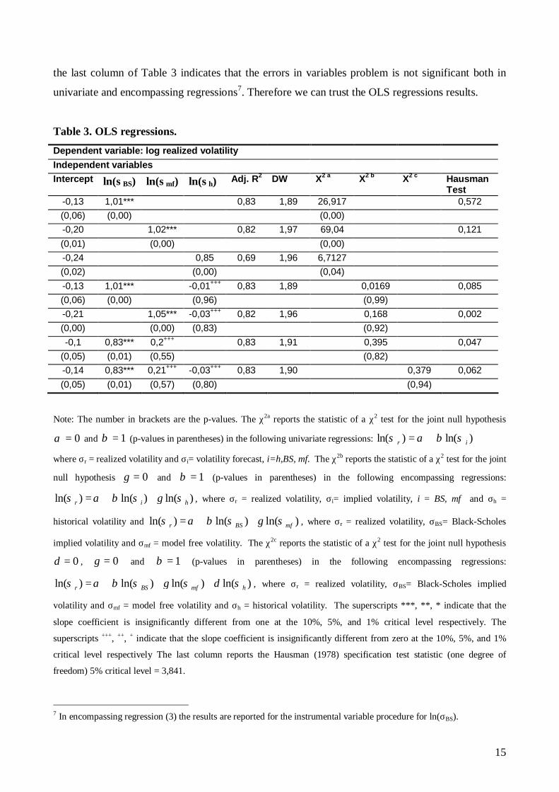
The results of the OLS univariate and encompassing regressions are reported in Table 3 (p-

values in parentheses). In all the regressions the residuals are homoscedastic and not autocorrelated

(the Durbin Watson statistic is not significantly different from two and the Breusch-Godfrey LM

test confirms non autocorrelation up to lag 125), although they are not normal6. Some comments are

in order. First of all, in all the three univariate regressions the beta coefficients are significantly

different from zero: this means that all the three volatility forecasts (Black-Scholes, model free and

historical) contain some information about future realised volatility. However, the null hypothesis

that any of the three volatility forecasts is an unbiased estimate of future realized volatility is

strongly rejected in all cases. In particular, in our sample, realized volatility is on average lower

than the two option based volatility forecasts, suggesting that option based forecasts overpredict

realised volatility. This is in line with the results found in Jiang and Tian (2005) and Lynch and

Panigirtzoglou (2003), that document a positive risk premium for stochastic volatility. As neither

one of the forecasts is unbiased we test if at least β is insignificantly different from one. The

hypothesis can not be rejected at the 10% critical level for the two option based estimates, while it

is strongly rejected for historical volatility. We can therefore consider both option based estimates

4 The Hausman specification test is defined as: ( )2ˆ ˆ

ˆ ˆ( ) ( )IV OLS

IV OLS

mVar Var

β β

β β

−=

− where: ˆ

IVβ is the beta obtained through

the Two Stage Least Squares procedure, ˆOLSβ is the beta obtained through the OLS procedure and Var(x) is the

variance of the coefficient x. The Hausman specification test is distributed as a χ2(1). 5 In the regressions that include as explanatory variable the lagged realised volatility, the Durbin’s alternative has been computed and it has confirmed the non autocorrelation of the residuals. The results of the Durbin’s alternative and of the Breusch-Godfrey LM test are available upon request.

6 The departure from normality of the residuals is not a result of ARCH effects: in all the regressions a test for ARCH effects on the residuals has been conducted that confirms the absence of autocorrelation in the squared residuals up to lag 12. Rather, it is caused by one outlier that corresponds to the September 2001 crash. In order to eliminate the effect of the outlier, regressions (5), (6), (7), (8) have been re-estimated on the sample period 26 September 2001- 31 December 2005 and the results, that are available upon request, are consistent with the ones reported for the entire sample period.

14

as unbiased after a constant adjustment given by the intercept of the regression. As for the adjusted

R2, among the two option-based volatility forecasts, the Black-Scholes volatility is ranked first in

explaining future realized volatility, strictly followed by the model free volatility, while historical

volatility has the lowest forecasting power.

Let us turn to the analysis of the encompassing regressions, in which we compare pairwise

two different volatility forecasts in order to understand if one of them subsumes all the information

contained in the other. First of all, we can observe that both option based volatility forecasts

subsume all the information contained in historical volatility. This is evident by comparing the

adjusted R2 of univariate and encompassing regressions and by looking at the coefficient of

historical volatility in the encompassing regressions. In fact, the inclusion of historical volatility

does not improve the goodness of fit according to the adjusted R2 and the coefficient of historical

volatility is not significantly different from zero in both regressions. Moreover, both option based

volatility forecasts are efficient and unbiased after a constant adjustment given by the intercept of

the regression. In fact the slope coefficients of both option based volatility forecasts are not

significantly different from one at the 10% level and the joint test of information content and

efficiency 0=γ and 1=β does not reject the null hypothesis for both option based volatility

forecasts.

In order to see if Black Scholes implied volatility subsumes all the information contained in

model free volatility, we test in encompassing regression (7) if 0=γ and 1=β . First of all, we

observe that only the slope coefficient of Black-Scholes implied volatility is significantly different

from zero, while the slope coefficient of model free volatility is not. Moreover, the joint test

0=γ and 1=β does not reject the null hypothesis, providing evidence for the superiority of Black-

Scholes implied volatility with respect to model free implied volatility.

For completeness, let us analyze the results of encompassing regression (8) in which we

compare all the three volatility forecasts. First of all, the inclusion of both model free volatility and

historical volatility doe not improve the goodness of fit given by the adjusted R2. In fact both the

coefficients of historical volatility and model free volatility are not statistically different from zero.

Moreover, also in this case Black-Scholes volatility is both efficient and unbiased after a

constant adjustment, as it is evident by looking at the χ2c column that jointly tests if 0δ = ,

0=γ and 1=β and does not reject the null hypothesis, providing evidence for the superiority of

Black-Scholes implied volatility with respect to both historical and model free volatility.

Finally, in order to test for robustness our results, and see if Black-Scholes implied volatility

or model free volatility have been measured with errors, we adopt an instrumental variable

procedure (IV) and run a two stage least squares. The Hausman (1978) specification test reported in

15

the last column of Table 3 indicates that the errors in variables problem is not significant both in

univariate and encompassing regressions7. Therefore we can trust the OLS regressions results.

Table 3. OLS regressions. Dependent variable: log realized volatility Independent variables Intercept ln(σBS) ln(σmf) ln(σh) Adj. R2 DW X2 a X2 b X2 c Hausman

Test -0,13 1,01*** 0,83 1,89 26,917 0,572 (0,06) (0,00) (0,00) -0,20 1,02*** 0,82 1,97 69,04 0,121 (0,01) (0,00) (0,00) -0,24 0,85 0,69 1,96 6,7127 (0,02) (0,00) (0,04) -0,13 1,01*** -0,01+++ 0,83 1,89 0,0169 0,085 (0,06) (0,00) (0,96) (0,99) -0,21 1,05*** -0,03+++ 0,82 1,96 0,168 0,002 (0,00) (0,00) (0,83) (0,92) -0,1 0,83*** 0,2+++ 0,83 1,91 0,395 0,047

(0,05) (0,01) (0,55) (0,82) -0,14 0,83*** 0,21+++ -0,03+++ 0,83 1,90 0,379 0,062 (0,05) (0,01) (0,57) (0,80) (0,94)

Note: The number in brackets are the p-values. The χ2a reports the statistic of a χ2 test for the joint null hypothesis

0=α and 1=β (p-values in parentheses) in the following univariate regressions: )ln()ln( ir σβασ +=

where σr = realized volatility and σi= volatility forecast, i=h,BS, mf. The χ2b reports the statistic of a χ2 test for the joint

null hypothesis 0=γ and 1=β (p-values in parentheses) in the following encompassing regressions:

ln( ) ln( ) ln( )r i hσ α β σ γ σ= + + , where σr = realized volatility, σi= implied volatility, i = BS, mf and σh =

historical volatility and ln( ) ln( ) ln( )r BS mfσ α β σ γ σ= + + , where σr = realized volatility, σBS= Black-Scholes

implied volatility and σmf = model free volatility. The χ2c reports the statistic of a χ2 test for the joint null hypothesis

0δ = , 0=γ and 1=β (p-values in parentheses) in the following encompassing regressions:

ln( ) ln( ) ln( ) ln( )r BS mf hσ α β σ γ σ δ σ= + + + , where σr = realized volatility, σBS= Black-Scholes implied

volatility and σmf = model free volatility and σh = historical volatility. The superscripts ***, **, * indicate that the

slope coefficient is insignificantly different from one at the 10%, 5%, and 1% critical level respectively. The

superscripts +++, ++, + indicate that the slope coefficient is insignificantly different from zero at the 10%, 5%, and 1%

critical level respectively The last column reports the Hausman (1978) specification test statistic (one degree of

freedom) 5% critical level = 3,841.

7 In encompassing regression (3) the results are reported for the instrumental variable procedure for ln(σBS).

16

Overall, these results point to a better performance of Black-Scholes implied volatility

versus model free volatility. These results are in line with Andersen and Bondarenko (2007). The

better performance of the Black Scholes volatility can be attributed to the fact that it has been

computed by using synchronous prices, from a vast set of options in a one hour window and it has

been computed as a weighted average of the two volatilities that correspond to the two strikes, one

above and one below the underlying asset with weights inversely proportional to the distance of the

strike price to the at the money strike. This better computational methodology has probably led the

Black-Scholes volatility to an improved forecasting performance with respect to previous papers

(see e.g. Christensen and Prabhala (1998)) in which non-syncronous prices were used and Black-

Scholes volatility were backed out from a single option. On the other hand, model free volatility

that has been computed by using all the cross section of option prices, obtains a good performance

that, however, is slightly worse than the simple Black-Scholes volatility. This is probably due to

some noise added by the hypotheses on the extrapolation of a continuum range of strike prices that

were necessary in order to compute the model free volatility. In particular, the lack of liquid options

in the tails of the strike price domain, and the assumption of a constant volatility equal to the one of

the nearest option strike may induce errors in the computation of the model free volatility. A

possible solution to this problem is investigated in the following section.

6. An alternative implementation of model free volatility.

The extrapolation method of Jiang and Tian (2005) is based on the extension of the domain of

strike prices by supposing that for strikes below the minimum value the implied volatility is

constant and equal to the volatility of Kmin, for strikes above the maximum value the implied

volatility is constant and equal to the volatility of Kmax. This assumption may introduce some bias in

the model free volatility estimation. Therefore in this section we compute model free volatility

without extending the domain of strike prices: we indicate this new estimate with model free

volatility 2 (σmf2). This is also in line with the computation methodology of the VIX volatility index

that uses only existing call and put options.

Descriptive statistics are reported in Table 4. We can see that on average σmf2 is greater than σBS

and lower than σmf, therefore it contains a lower volatility risk premium than σmf. Given that the

natural logarithm of the series conforms more to normality, we use the latter in the regressions.

We run both univariate regression (5) and encompassing regressions (6), (7) and (8) in order to

investigate the performance of this different model free volatility estimate, in predicting future

realized volatility. The results are reported in Table 5.

17

Table 4. Descriptive statistics for σmf2.

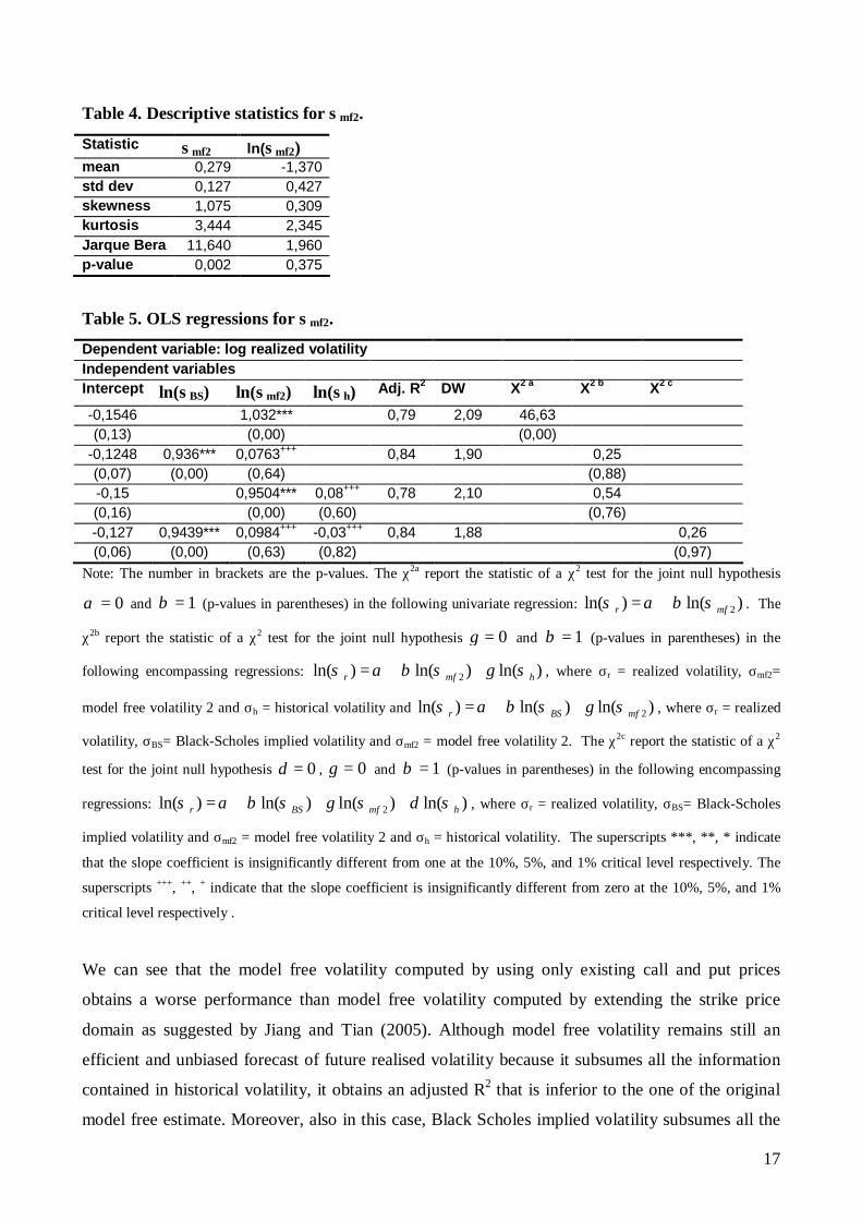
Statistic σmf2 ln(σmf2) mean 0,279 -1,370 std dev 0,127 0,427 skewness 1,075 0,309 kurtosis 3,444 2,345 Jarque Bera 11,640 1,960 p-value 0,002 0,375

Table 5. OLS regressions for σmf2.

Dependent variable: log realized volatility Independent variables Intercept ln(σBS) ln(σmf2) ln(σh) Adj. R2 DW X2 a X2 b X2 c

-0,1546 1,032*** 0,79 2,09 46,63 (0,13) (0,00) (0,00)

-0,1248 0,936*** 0,0763+++ 0,84 1,90 0,25 (0,07) (0,00) (0,64) (0,88) -0,15 0,9504*** 0,08+++ 0,78 2,10 0,54 (0,16) (0,00) (0,60) (0,76) -0,127 0,9439*** 0,0984+++ -0,03+++ 0,84 1,88 0,26 (0,06) (0,00) (0,63) (0,82) (0,97)

Note: The number in brackets are the p-values. The χ2a report the statistic of a χ2 test for the joint null hypothesis

0=α and 1=β (p-values in parentheses) in the following univariate regression: 2ln( ) ln( )r mfσ α β σ= + . The

χ2b report the statistic of a χ2 test for the joint null hypothesis 0=γ and 1=β (p-values in parentheses) in the

following encompassing regressions: 2ln( ) ln( ) ln( )r mf hσ α β σ γ σ= + + , where σr = realized volatility, σmf2=

model free volatility 2 and σh = historical volatility and 2ln( ) ln( ) ln( )r BS mfσ α β σ γ σ= + + , where σr = realized

volatility, σBS= Black-Scholes implied volatility and σmf2 = model free volatility 2. The χ2c report the statistic of a χ2

test for the joint null hypothesis 0δ = , 0=γ and 1=β (p-values in parentheses) in the following encompassing

regressions: 2ln( ) ln( ) ln( ) ln( )r BS mf hσ α β σ γ σ δ σ= + + + , where σr = realized volatility, σBS= Black-Scholes

implied volatility and σmf2 = model free volatility 2 and σh = historical volatility. The superscripts ***, **, * indicate

that the slope coefficient is insignificantly different from one at the 10%, 5%, and 1% critical level respectively. The

superscripts +++, ++, + indicate that the slope coefficient is insignificantly different from zero at the 10%, 5%, and 1%

critical level respectively .

We can see that the model free volatility computed by using only existing call and put prices

obtains a worse performance than model free volatility computed by extending the strike price

domain as suggested by Jiang and Tian (2005). Although model free volatility remains still an

efficient and unbiased forecast of future realised volatility because it subsumes all the information

contained in historical volatility, it obtains an adjusted R2 that is inferior to the one of the original

model free estimate. Moreover, also in this case, Black Scholes implied volatility subsumes all the

18

information contained in this latter model free estimate. Therefore we can conclude that even if the

Jiang and Tian (2005) extrapolation method is based on particular assumptions on the smile shape

outside the existing strike price interval, it is superior to a methodology that uses only the existing

strike price domain.

7. Conclusions.

The forecasting performance of Black Scholes implied volatility versus a time series volatility

forecast has been extensively analysed in various papers. In most cases Black Scholes implied

volatility is extracted from at the money options. Only a few papers have addressed the issue of

investigating the forecasting performance of a different option based volatility forecast: model free

implied volatility. Model free implied volatility is completely specified by a continuum set of

option prices expiring on date T. As it is derived by using a cross section of option prices differing

in strike prices and option type, it should be, theoretically, more informative than implied volatility

backed out from a single option. However, due to numerous practical limitations (limited number of

strike prices, that are available only at fixed increments), the evidence about the superiority of

model free implied volatility versus Black-Scholes implied volatility is mixed (see e.g. Jiang and

Tian (2005), Andersen and Bondarenko (2007)).

In this paper we have investigated the forecasting power of the two option based volatility

forecasts: Black-Scholes implied volatility and model free volatility. As Black and Scholes implied

volatility differs depending on strike price of the option (the so-called smile effect) and, due to

measurement errors, option type (call versus put), which option class yields implied volatilities that

are most representative of the markets’ volatility expectations is still an open debate. In order to

pursue a fair comparison with model free implied volatility, that is derived based on a cross section

of option prices, for implied volatility we have used a weighted average of implied volatilities

backed out from different option classes.

Two hypotheses have been tested: unbiasedness and efficiency of the different volatility

forecasts. Our results suggest that both option based volatility forecasts contain more information

about future realised volatility than historical volatility. They are not unbiased, since they contain a

substantial risk premium, but they can be considered unbiased after a constant adjustment given by

the intercept of the regression. Moreover they are both efficient forecasts of realised volatility in

that they subsume all the information contained in historical volatility.

The comparison between the two option based volatility forecasts has highlighted a slightly

better performance of Black-Scholes implied volatility versus model free volatility. These results

are in line with the finding of Andersen and Bondarenko (2007) that found that Black and Scholes

19

implied volatility obtains a better forecasting performance than model free volatility, being less

sensitive to the time variation in the volatility risk premium.

The better performance of the Black Scholes volatility can be attributed to the fact that it has

been computed by using synchronous prices, from a vast set of options in a one hour window and it

has been computed as a weighted average of the two volatilities that correspond to the two strikes,

one above and one below the underlying asset, with weights inversely proportional to the distance

of the strike price to the at the money strike. This better computational methodology has probably

led the Black-Scholes volatility to an improved forecasting performance with respect to previous

papers (see e.g. Christensen and Prabhala (1998)) in which non-syncronous prices were used and

Black-Scholes volatility were backed out from a single option. On the other hand, model free

volatility, that has been computed by using all the cross section of option prices, obtains a good

performance that, however, is slightly worse than the simple Black-Scholes volatility. This is

probably due to some noise added by the hypotheses on the extrapolation of a continuum range of

strike prices that were necessary in order to compute the model free volatility. In particular, the lack

of liquid options in the tails of the strike price domain, and the assumption of a constant volatility

equal to the one of the nearest option strike may have induced errors in the computation of the

model free volatility. One possible solution to reduce the impact of this latter assumption would be

to use only the existing strike price domain, as it is done for the computation of the VIX index.

However, this tactic has proved to be inferior, in the present dataset, to the extrapolation

methodology proposed by Jiang and Tian (2005). The study of other possible remedies in order to

improve the model free volatility performance is left for future research.

20

Appendix 1.

In order to examine the performance of model free implied volatility when we vary the parameters u

and ∆K, we show some simulations based on the Heston’s (1993) stochastic volatility model.

In the Heston model the underlying asset follows the stochastic process:

1/ 2tt t

t

dS dt V dWS

µ= +

The variance of the underlying asset follows the mean reverting process: 1/ 2( )t

vt v v t v tdV k V dt V dWθ σ= − +

with: v

t tdW dW dtρ=

Vt is the variance of the returns of the underlying asset, Wt and vtW are the standard Wiener

processes for the underlying and the variance with correlation ρ , θ is the long run average of

variance, k is the mean reversion rate, vσ is the volatility of variance.

For the present implementation we use the same parameters as in Heston (1993), namely: spot price

S=100, risk free rate r=0, time to maturity τ=0,5, current variance v=0,01, correlation ρ =-0,5,

mean reversion rate k=2, long run average of variance θ =0,01, volatility of variance vσ =0,225,

price of volatility risk λ=0. The volatility of the stock returns over the life time of the option is

0,071. For the current implementation we generate call and put option prices, by using the Heston

model for a range of strike prices K=[80,120] equally spaced by ∆K=0,5. For this interval of

strikes, we analyse both the truncation and the discretization errors by computing the model free

volatility by using different values of u and ∆K and deriving the percentage error (PE) in predicting

the true volatility of 0,071, as: 0,071

0,071mfPE

σ−= . Recall that the parameter u determines the range

of strike prices used, while ∆K sets the spacing between strike prices.

In order to examine the truncation error we compute the model free volatility by using different

levels of u and a fixed ∆K=0,5. The results are reported in Table A1.1: u determines the strike

price range used [Kmin, Kmax], σmf is the model free volatility and PE is the percentage error in

predicting the true volatility of 0,071, that is computed as: 0,071

0,071mfPE

σ−= . We can see that the

truncation error is substantially high only if we use a very narrow interval of strikes: increasing the

21

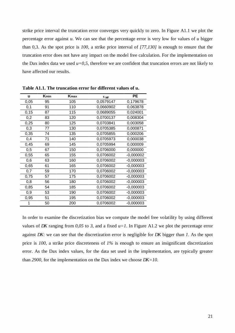
strike price interval the truncation error converges very quickly to zero. In Figure A1.1 we plot the

percentage error against u. We can see that the percentage error is very low for values of u bigger

than 0,3. As the spot price is 100, a strike price interval of [77,130] is enough to ensure that the

truncation error does not have any impact on the model free calculation. For the implementation on

the Dax index data we used u=0,5, therefore we are confident that truncation errors are not likely to

have affected our results.

Table A1.1. The truncation error for different values of u. u Kmin Kmax σMF PE

0,05 95 105 0,0579147 0,179678 0,1 91 110 0,0660902 0,063878

0,15 87 115 0,0689055 0,024001 0,2 83 120 0,0700137 0,008304

0,25 80 125 0,0703841 0,003058 0,3 77 130 0,0705385 0,000871

0,35 74 135 0,0705855 0,000206 0,4 71 140 0,0705973 0,000038

0,45 69 145 0,0705994 0,000009 0,5 67 150 0,0706000 0,000000

0,55 65 155 0,0706002 -0,000002 0,6 63 160 0,0706002 -0,000003

0,65 61 165 0,0706002 -0,000003 0,7 59 170 0,0706002 -0,000003

0,75 57 175 0,0706002 -0,000003 0,8 56 180 0,0706002 -0,000003

0,85 54 185 0,0706002 -0,000003 0,9 53 190 0,0706002 -0,000003

0,95 51 195 0,0706002 -0,000003 1 50 200 0,0706002 -0,000003

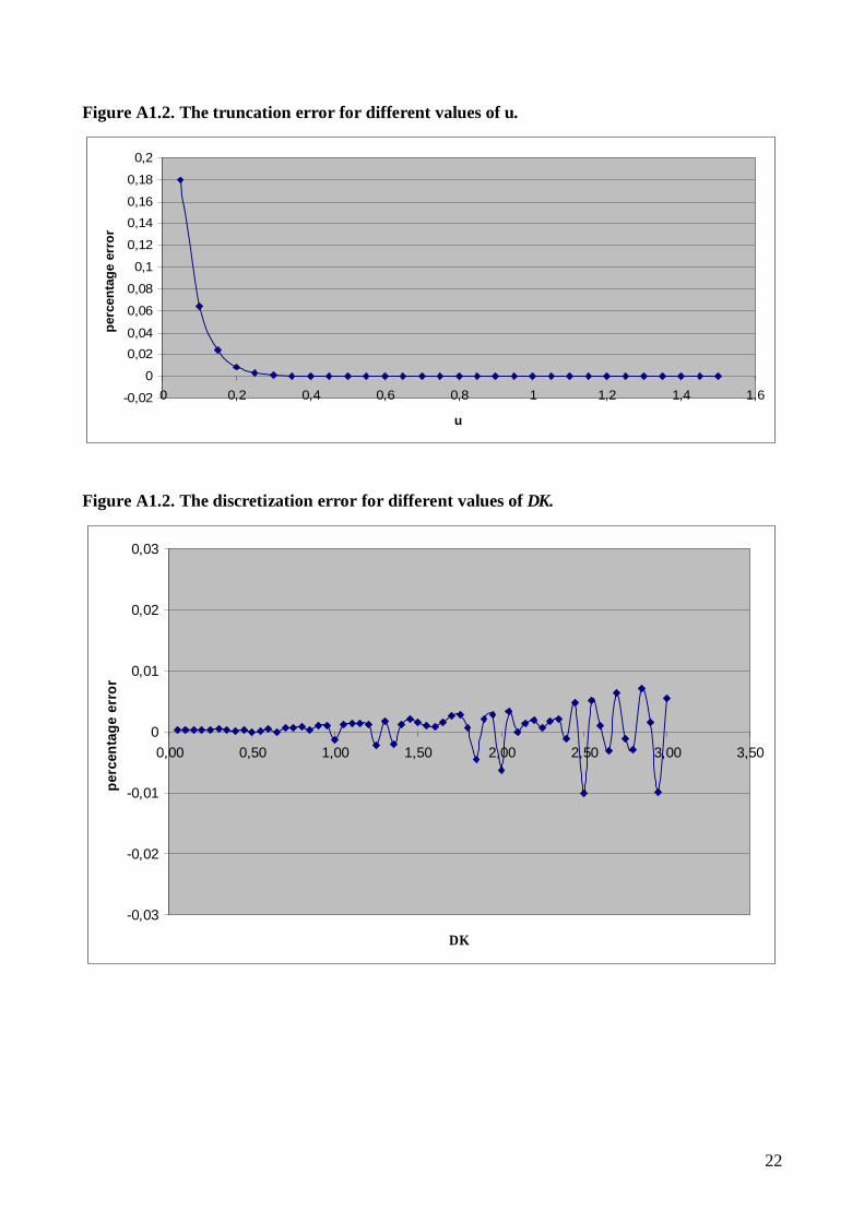
In order to examine the discretization bias we compute the model free volatility by using different

values of ∆K ranging from 0,05 to 3, and a fixed u=1. In Figure A1.2 we plot the percentage error

against ∆K: we can see that the discretization error is negligible for ∆K bigger than 1. As the spot

price is 100, a strike price discreteness of 1% is enough to ensure an insignificant discretization

error. As the Dax index values, for the data set used in the implementation, are typically greater

than 2900, for the implementation on the Dax index we choose ∆K=10.

22

Figure A1.2. The truncation error for different values of u.

-0,02

0

0,020,04

0,06

0,08

0,1

0,12

0,140,16

0,18

0,2

0 0,2 0,4 0,6 0,8 1 1,2 1,4 1,6

u

perc

enta

ge e

rror

Figure A1.2. The discretization error for different values of ∆K.

-0,03

-0,02

-0,01

0

0,01

0,02

0,03

0,00 0,50 1,00 1,50 2,00 2,50 3,00 3,50

∆ Κ

perc

enta

ge e

rror

23

References.

1. Ait-Sahalia, Y., A.W. Lo, 1998. Non parametric estimation of state-pric densities implicit in

financial asset prices. Journal of Finance 53, 499-547.

2. Andersen T.G., T. Bollerslev, 1998. Answering the skeptics: Yes, standard volatility models

do provide accurate forecasts. International Economic Review, 39, 885-905

3. Andersen T.G., T. Bollerslev, F.X. Dieblod, P. Labys, 2001. the distribution of realised

exchange rate volatility. Journal of the American Statistical Association, 96, 42-55.

4. Andersen T.G., O. Bondarenko, 2007. Construction and interpretation of model free implied

volatility. NBER Working Paper Series, working paper n. 13449.

5. Bandi F.M., B. Perron, 2006. Long Memory and the Relation Between Implied and Realized

Volatility. Journal of Financial Econometrics 4, 636-670.

6. Bates, D., 1991. The crash of ’87: was it expected? The evidence from options markets.

Journal of Finance, 46, 1009-1044.

7. Black F., M. Scholes, 1973. The pricing of options and corporate liabilities. Journal of

Political Economy 81, 637-654.

8. Blair B.J., Poon S., Taylor S.J., 2001. Modelling S&P100 volatility: the information content

of stock returns. Journal of Banking and Finance 25, 1665-1679.

9. Bollerslev T., Ray Y. Chou, Kenneth P. Kroner, 1992. ARCh modelling in finance: A

review of the theory and empirical evidence. Journal of Econometrics 52, 5-59.

10. Britten-Jones, M., A. Neuberger, 2000. Option prices, implied price processes and stochastic

volatility. Journal of Finance, 55, 839-866.

11. Campa, J.M., K.P. Chang, R.L. Reider, 1998. Implied exchange rate distributions: evidence

from OTC option markets. Journal of International Money and Finance, 17, 117-160.

12. Canina, L., Figlewski S., 1993. The informational content of implied volatility. Review of

Financial studies 6 (3) 659-681.

13. Carr P., L. Wu, 2006. A tale of two indices. The Journal of Derivatives, Spring.

14. Christensen B.J., C.S. Hansen 2002. New evidence on the implied-realized volatility

relation. The European Journal of Finance, 8, 187-205.

15. Christensen B.J., C. S. Hansen, N.R. Prabhala. 2001. The telescoping overlap problem in

options data. Working paper, University of Aarhus and University of Maryland.

16. Christensen B.J., N.R. Prabhala. 1998. The relation between implied and realized volatility.

Journal of Financial Economics, 50, 125-150.

24

17. Day T.E., Lewis C.M., 1992. Stock market volatility and the informational content of stock

index options. Journal of Econometrics, 52, 267-287.

18. Ederington L. H., W. Guan. 2002. Is implied volatility an informationally efficient and

effective predictor of future volatility? Journal of Risk 4 (3), 29-46.

19. Ederington L., W. Guan. 2005. The information frown in option prices. Journal of Banking

and Finance, 29, 1429-1457.

20. Fleming, J. 1998. The quality of market volatility forecasts implied by S&P100 index option

prices. Journal of Empirical Finance, 5 (4), 317-345.

21. Ghysels, E., A. Harvey, E. Renault, 1996. Stochastic volatility. In Handbook of Statistics:

Statistical Methods in Finance, 14, Maddala and C. R. Rao eds. Amsterdam, Elsevier

Science, 119-191.

22. Godbey J.M., J.W. Mahar. 2007. Forecasting power of implied volatility: evidence from

individual equities. B>Quest, University of West Georgia.

23. Heston S.L., 1993. A closed form solution for options with stochastic volatility with

application to bond and currency options. The Review of Financial Studies, 6 (2) 327-343.

24. Jang G. J., Y. S. Tian, 2005. Model free implied volatility and its information content. The

Review of Financial Studies, 18 ( 4) 1305-1342.

25. Jorion, P., 1995. Predicting volatility in the foreign exchange market. Journal of Finance 50

(2) 507-528.

26. Lamourex C.G., W.D. Lastrapes, 1993. Forecasting stock-return variance: toward an

understanding of stochastic implied volatilities. Review of Financial Studies 6 (2) 293, 326.

27. Lynch D., N. Panigirtzoglou. 2003. Options implied and realised measures of variance.

Working paper Monetary Instruments and Markets Division, Bank of England.

28. Moriggia V., S. Muzzioli, C. Torricelli, 2007. Call and put implied volatilities and the

derivation of option implied trees. Frontiers in Finance and Economics 4 (1) 35-64.

29. Poon S., C.W. Granger. 2003. Forecasting volatility in financial markets: a review. Journal

of Economic Literature, 41, 478-539.

30. Shimko, D., 1993. Bounds of probability. Risk, 6, 33-37.

31. Szakmary A, Evren Ors, Jin Kyoung Kim, Wallace N Davidson. 2003. The predictive power

of implied volatility: evidence from 35 futures markets. Journal of Banking and Finance 27,

2151-2175.