Option-Based Credit Spreads - Booth School of...

Option-Based Credit Spreads

On-Line Technical Appendix

Christopher L. Culp

Johns Hopkins Institute for Applied Economics

and Swiss Finance Institute

Yoshio Nozawa

Federal Reserve Board

Pietro Veronesi

University of Chicago, NBER, and CEPR

This Technical Appendix contains additional material that did not find space in the maintext. The Appendix is divided in five sections:

A. Data description and filters

B. Default frequencies from Moody’s data

C. Methodology

D. Extensions and Robustness

E. Tables and figures

Appendix A. Data Description and Filters.

Equity Prices and Accounting Variables. We obtain stock prices and accounting in-

formation from the Center for Research in Security Prices (CRSP). We use returns in the

postwar period (1946 - 2013) to compute asset returns and ex ante default probabilities for

our pseudo firms, as explained in the text.

Risk-Free Securities. We construct the risk-free zero-coupon bonds from 1-, 3-, and 6-

month T-bill rates and 1-, 2-, and 3-year constant maturity Treasury yields obtained from

the Federal Reserve Economic Data (FRED) database. We convert constant maturity yields

into zero-coupon yields and linearly interpolate to match option maturities. We also obtain

1

commercial paper rates from FRED, which we use to compute credit spreads for short-term

debt.

Corporate Bonds. We construct the panel data of corporate bond prices from the Lehman

Brothers Fixed Income Database, TRACE, the Mergent FISD/NAIC Database, and DataS-

tream, prioritized in this order when there are overlaps among the four databases. Detailed

descriptions of these databases and the effects of prioritization are discussed in Nozawa

(2016). In addition, we remove bonds with floating coupon rates and/or embedded option

features other than callable bonds.

As call options embedded in corporate bonds bias credit spreads on these bonds up, we

adjust the call premium based on regressions. Specifically, we follow Gilchrist and Zakrajsek

(2012) (GZ) to estimate the value of embedded call options using both callable and non-

callable bonds. We run a panel regression,

log si,t = b0Callablei + b1CallableiXi,t + b2Zi,t + εi,t,

where si,t is credit spread, Callablei is a dummy variable for a callable bond, Xi,t is a vector of

bond characteristics that affect call premiums, and Zi,t is a measure of default risk, motivated

by the Merton model.

Following the spirit of GZ, we include seven credit rating dummies (Aaa, Aa, A, Baa, Ba,

B, Caa-), log duration, log par amount outstanding, log coupon rate, log age, the first three

principal components of Treasury yield curves, and 1-year rolling volatility of daily changes

in 10-year Treasury yield in the characteristic vector Xi,t. For the default risk measure Zi,t,

we include Merton’s Distance to Default (DD), log duration, log par amount outstanding,

log coupon rate, log age, three industry dummies based on FISD industry classification

(financial, utility, industrials), and seven credit rating dummies.

There are two major differences between our specification and GZ’s. First, we use all

bonds with maturities from 1 month to 2.5 years, including the ones issued by private firms,

for which information about balance sheet and stock prices is not available. We use bonds

issued by private firms to maximize the number of observations, as we look at finely classified

data based on credit ratings and maturity instead of aggregate data. Because we do not

have DD measures for such bonds, we populate the missing data by the average DD for a

month for each rating.

Second, we truncate credit spreads at the 1st and 99th percentiles of the distribution, as

compared to GZ’s truncation at 0.05% and 35%. The truncation at the 1st percentile rather

than 0.05% is necessary for us to estimate Aaa/Aa-rated spreads precisely, as some of these

2

bonds, especially ones with very short maturity, have spreads below 0.05% including some

negative values. Thus, we transform the credit spreads by

s = s − min(s) + 0.01,

and take logarithm of transformed spreads to run the regression.

The first two columns of Table A1 show the estimated slope coefficients of the regression.

As expected, bonds with high default risk (DD), longer duration, greater size, larger coupon

rate, and long age have higher credit spreads. The call premium is greater for bonds with

longer duration, larger coupon rate, when the level of risk-free rates are low (low PC1), or

when volatility is high. In addition, call premiums (as a fraction of credit spreads) are larger

for IG bonds than HY bonds.

Based on these estimates, we adjust corporate credit spreads on callable bonds in our

sample. Specifically, we use adjusted spreads for callable bonds, calculated as follows:

sadji,t = exp (log si,t − b0 − b1Xi,t) + min (s) − 0.01.

The resulting adjustments for credit spreads are non-trivial, as the 10th, 50th and 90th

percentile differences of, si,t − sadji,t , are 0%, 0.41% and 1.38%, respectively. These estimates

for call premiums are large because we estimate the regression only using short-term bonds.

As reported in the third and fourth columns of Table A1, when we include bonds with

all maturities, the median call premium falls to 0.10%, which is close to the value Huang

and Huang (2012) use to adjust for call premiums. Our regression specification leads to

conservative estimates for call premiums. When we estimate the regression following GZ

(truncating at 0.05% and 35%, use public firms only, use all maturities above one year), the

median call premiums rise to 0.22%.

Credit Default Swaps. We obtained five-year CDX indices for the investment-grade

CDX.IG and high yield CDX.HY from JP Morgan and single-name CDS spreads from

Markit. The samples start in November 2001 and April 2003 for CDX.HY and CDX.IG,

respectively, and end in August 2014.

Stock Options. We use the OptionMetrics Ivy DB database for daily prices on SPX index

options and options on individual stocks from January 4, 1996, through August 31, 2014. In

addition, we use SPX options from the MDR data of Market Data Express to cover the 1990

to 1995 sample. To minimize the effects of quotation errors in SPX options, we generally

follow Constantinides, Jackwerth, and Savov (2013) (CJS) to filter the data. As in CJS, we

apply the filters only to the prices to buy – not to the prices to sell – so that our portfolio

3

formation strategy is feasible for real-time investors. As in CJS, we apply the following

specific filters:

1. Level 1 Filters: We remove all but one of any duplicate observations. If there are

quotes with identical contract terms but different prices, we pick the quote with the

implied volatility (IV) closest to that of the moneyness of its neighbors and remove the

others. We also remove the quotes with bids of zero.

2. Level 2 and Level 3 Filters: Because we need quotes for long-term, deep out-of-the-

money puts and deep in-the-money calls, we do not apply filters based on moneyness

or maturity, but we remove all options with zero open interest. Following CJS, we also

remove options with less than seven days to maturity. We also apply “implied interest

rate < 0,” “unable to compute IV,” “IV,” and “put-call parity” filters.1

For individual equity options that are typically American style, put-call parity only holds

as an inequality and we thus apply a different set of filters. We follow Frazzini and Pedersen

(2012) to detect likely data errors and drop all observations for which the ask price is lower

than the bid price and the bid price is equal to zero. In addition, we require options to

have positive open interest, and non-missing delta, IV, and spot price. We also drop options

violating the put-call parity bounds for American options, and basic arbitrage bounds of a

non-negative “time value” P-V where V is the option “intrinsic value’ equal to max(K−S, 0)

for puts and P is the option’s price. We then drop equity options with a time value (P−V )/P

(in percentage of option value) below 5%, as the low time value tends to lead to early exercise.

Furthermore, to mitigate the effect of the outliers, we drop options with embedded leverage,∂P∂S

SP, in the top or bottom 1% of the distribution. Finally, we drop the options on the firms

whose µt,τ and σt,τ are in the top or bottom 5% of the distribution.

Commodity Futures and Options. We obtain monthly settlement prices for commodity

futures option for light, sweet crude oil, natural gas (Henry Hub), gold, corn, and soybeans

from CME Group. The sample periods vary depending on the underlying commodity futures

contracts, and are shown in Table A2. We also obtain the underlying futures settlement

prices from CME, and spot prices from Global Financial Data. The expiry date for futures

is close to that of options (typically they are apart less than a month), and we assume for

1The “implied interest rate <0” filter removes options with negative interest rates implied by put-callparity. The “unable to compute IV” filter removes options that imply negative time value. The “IV” filterremoves options for which implied volatility is one standard deviation away from the average among thepeers. In this case, the peer group is defined by the bins of moneyness with a width of 0.05. The “put-callparity” filter removes options for which the put-call parity implied interest rate is more than one standarddeviation away from the average among the peers.

4

our analysis that they expire at the same time. We use the convenience yield backed out

from spot and futures prices as a predictor to compute the ex ante probabilities of default.

CME commodity futures options are American options, but we treat them as European

in computing pseudo bond prices because they are so deep out-of-the-money that the early

exercise premium is likely negligible. We remove the observations if i) the price does not

satisfy the put-call parity bound, ii) open interest is zero, or iii) the number of days to

maturity is less than or equal to seven days. In computing the put-call parity bound, we

use LIBOR and swap rates obtained from FRED and Barclays, while the pseudo bond prices

are computed based on Treasury yields. (We use swap rates to compute the put-call parity

bound, since CJS show that the risk-free rate that investors use to evaluate options is higher

than T-bill rate.)

Currency Futures and Options. We use two different datasets.

1. We obtain prices for currency futures options for GBP, EUR, JPY, CHF, AUD and

CAD from CME, and the corresponding spot exchange rates from Global Financial

Data. We apply the same cleaning procedure as we do for the other commodity

futures options, as described above.

2. We also use the monthly physical currency option data from JP Morgan for 9 currencies

(CAD, EUR, NOK, GBP, SEK, CHF, AUD, JPY and NZD) from 1999 to 2014. The

exchange rates are relative to US dollar. The quoted implied volatility for 1-, 3-, 6-, 12-

and 24-month options are used to compute currency option prices. The strike prices

for currency options are expressed in terms of deltas, and we use at-the-money (50-

delta) options, 10-delta calls and puts, and 25-delta calls and puts. When converting

implied volatilities into prices, we follow Jurek (2014) and use LIBOR and swap rates

for each currency. The pricing of pseudo bonds are computed based on US Treasury

yields (FRED). To estimate the ex ante and ex post probabilities of default, we also

use spot exchange rates obtained from JP Morgan.

Swaptions. We use monthly swaption price data obtained from ICAP from July 2002

through December 2014. The data provides the premium for the right to enter an in-

terest rate swap contract (in USD) in which investors pay or receive a fixed rate in ex-

change for 3-month LIBOR. We use the option expiries of 3, 6, 12 and 24 months on

swaps with 5-, 10- and 20-year tenors. The available strike prices are at-the-money and

±300,±200,±150,±100,±75,±50,±25,±12.5 basis points from the at-the-money swap rate.

The option premiums in the data are end-of-the-day aggregate quotes in the interdealer bro-

5

ker market in which ICAP is a major participant. To compute the underlying forward swap

rate, we use the swap rate from JP Morgan.

Appendix B. Default Frequencies for Real Corporate Bonds.

As explained in the text, our goal is to construct pseudo bonds that match the realized

default frequencies of the actual corporate bonds used as our main empirical benchmark.

To that end, we employ a large dataset of corporate defaults spanning the 44-year period

from 1970 to 2013 obtained from Moody’s Default and Recovery Database. For each credit

rating assigned by Moody’s to our universe of firms, we estimate ex post default frequencies

at various horizons from 30 days up to two years. We use our own estimates rather than the

original Moody’s default frequencies for three main reasons. First, we are interested in the

variation of default frequencies over the business cycle, whereas Moody’s historical default

frequencies are only available as unconditional averages. Second, we are interested in the

default frequencies at horizons of below one year, and default frequencies are not provided

by Moody’s for such short time horizons. And third, we need default frequencies for coarser

categories (such as Aaa/Aa, A/Baa) as options’ strike prices often lack sufficient granularity

to differentiate across such credit ratings.

Table A3 reports historical default rates from 1970 through 2013 from our sample of firms

across credit rating categories and time horizons. We compute historical default frequencies

separately for international and U.S. firms. Our results are directly comparable to Moody’s

historical default rates (reported in Moody’s (2014)) for one- and two-year horizons. As

Table A3 shows, our estimated default rates closely match the Moody’s global default rates

for those horizons.

The last two columns of Table A3 report default rates for U.S. firms in NBER-dated

booms and recessions. Predictably, we find that default frequencies are higher in recessions

than in booms across all credit ratings. At the 1-year horizon, for instance, A-rated bonds

have a default frequency of only 0.02% in booms but 0.13% in recessions (as compared to

an unconditional U.S. average of 0.04%). Default frequencies for speculative-grade bonds

also show large variations over the business cycle. For example, a B-rated bond has a 3.57%

default rate at the 1-year horizon during booms but more than twice that in recessions (as

compared to an unconditional average of 4.01%).

Table A3 also shows default frequencies at short horizons of 30, 91, and 183 days. At the

30-day horizon, all IG bonds have essentially zero historical default frequencies (although,

6

in recessions, the historical default rate ticks up 0.01% for bonds rated A- and Baa). Some

more action for these bonds is observable at the 91- and 183-day horizons, especially during

recessions. For example, Baa-rated bonds have defaulted with 0.04% and 0.12% frequencies

at the 91- and 183-day horizons (respectively) during recessions, which are much higher than

the corresponding unconditional default frequencies of 0.02% and 0.05%. HY bonds, by

contrast, exhibit relatively substantial historical default activity even at short horizons. For

instance, B-rated bonds have 0.22%, 0.75%, and 1.69% unconditional default frequencies over

30, 91, and 183 days, respectively, which increase to 0.43%, 1.48%, and 3.33%, respectively,

during recessions.

Appendix C. Methodology.

C.1. Ex Ante Default Probabilities

In this section we describe in detail the methodology to compute ex ante default proba-

bilities for pseudo bonds, that we summarize in Section 2.2. of the text.

At every time t and for each bond with maturity τ and face value Ki,t, we want to

compute

pt(τ ) = Pr [Ai,t+τ < Ki,t |Ft ] (9)

where Ft denotes the information available at time t.

To avoid making explicit distributional assumptions about asset returns and to keep

our approach as model-free as possible, we use the empirical distribution of underlying asset

values to compute pt(τ ). Nevertheless, we need to take into account any time-varying market

conditions, which could have a substantial impact on default probabilities for a given current

market leverage ratio Li,t = Ki,t/At.

When pseudo firm i’s assets consist solely of the SPX, the market value of the firm’s

assets at time t is Ai,t = SPX. Dropping the subscript i for notational simplicity, let log

asset growth for this firm be given by:

ln(

At+τ

At

)= µt,τ + σt,τεt+τ (10)

where εt+τ are standardized unexpected asset returns. Because we do not impose any distri-

butional assumption on εt+τ , this is just a statement that log asset growth ln (At+τ/At) has

an expected component and a volatility scaling parameter σt,τ .

7

A structural assumption is required to estimate µt,τ and σt,τ . Accordingly, we estimate

µt,τ by running return forecasting regressions (excluding dividends) using the dividend-price

ratio for τ horizons, and σt,τ by fitting a GARCH(1,1) process based on monthly asset

returns.2 Given estimates of µt,τ and σt,τ , we collect the (overlapping) history of shocks

εt+τ =ln (At+τ/At) − µt,τ

σt,τ

and use the empirical distributions of these shocks to compute empirical default probabilities

for each leverage ratio Li,t at any given time t.

In particular, we rewrite the probability pt(τ ) in (9) as follows:

pt(τ ) = Pr [εt+τ < Xi,t| Ft] where Xi,t =ln (Li,t) − µt,τ

σt,τ(11)

Thus, we can estimate such probabilities simply as:

pt(τ ) =n(εs+τ < Xi,t)

n(εs+τ )for all s + τ < t. (12)

where n(x) counts the number of events x. We perform these computations on expanding

windows, so that at any time t we only use information available at time t to predict the

default probability of a pseudo bond with maturity t+τ . The empirical distribution of shocks

εt+τ thus determines these default probabilities. Panel A of Figure A1 presents the histogram

of shocks {εt+τ} for maturity τ = 2. The Kolmogorov-Smirnov test rejects normality at 1%

confidence level.

To illustrate, Panel D of Figure 1 in the paper plots the default probabilities of the two

SPX pseudo bonds in Panel A. The high-leverage pseudo firm has higher default probability

than the low-leverage pseudo firm, which is not surprising because both pseudo firms have

the same underlying assets, the SPX. (As we shall see, when firms differ from the type of

underlying assets, firms with the same leverage may have different default probabilities due

to different underlying assets’ characteristics). Both default probabilities increased during

the financial crisis, with the high-leverage pseudo bond jumping to almost 100% and hovering

around that value up to maturity. The default probability of the low-leverage bond returned

to zero by maturity, as it became clear that no default would occur.

We extend the above procedure to the case of single-stock pseudo bonds. When pseudo

firm i’s assets Ai,t consist of shares of an individual stock included in the SPX, we must take

into account survivorship bias – i.e., if at time t a given stock is part of the SPX, it must have

2Specifically, we use monthly returns to estimate σ2t,1 and compute σ2

t,τ for τ > 1 from the properties ofthe fitted GARCH(1,1) model.

8

done well in the past and thus its shocks are biased upwards. To avoid survivorship bias,

for every t we consider the full cross-section of all firms underlying the SPX index before t

(including those that dropped out of the index). For each firm i and s < t, we use its previous-

year return volatility and unconditional average return (before s) to compute its normalized

return shock. We then use the full empirical distribution of all these normalized shocks across

firms i for all s < t to obtain the default probabilities for each bond issued by each pseudo

firm j as of time t. As before, for each firm j we scale the shocks by their unconditional means

and previous-year volatilities. Panel B of Figure A1 shows the histogram of the resulting

normalized shocks. These shocks display fat tails, and the Kolmogorov-Smirnov test rejects

normality at the 1% confidence level.

C.2. Pseudo Ratings of Pseudo Bonds

In this section we describe the results of the pseudo rating assignment for two-year pseudo

bonds introduced in Section 2.2. of the text.

Panel A of Table A4 presents the default frequencies, both average and over the business

cycle, estimated from Moody’s dataset on corporate defaults for the credit ratings reported

in the first column. The last two columns report break points in booms and recessions,

computed as the middle points of the corresponding default probabilities in columns three

and four.3 So, for every month t, we compare the probability of each bond i, pi,t(τ ), to the

corresponding thresholds in the last two columns, depending on whether month t is a boom

or recession, and obtain a classification into a pseudo rating category.

Panels B and C report the results of our pseudo rating classification methodology for

pseudo bonds based on single stocks and the SPX, respectively. In both panels, for each

rating in the first column, the second and the third columns show the weighted average

ex ante default probabilities for pseudo bonds in each rating category. According to the

procedure, these probabilities should be close to the historical default frequencies reported

in columns three and four of Panel A, and indeed they are. Columns four to six of Panels B

and C of Table A4 test whether ex post default frequencies are close to the ex ante default

probabilities. We cannot reject that ex ante and ex post default probabilities are equivalent.

The second-to-last column in Panels B and C reports the average moneyness of the

options (K/A). The options used for highly rated pseudo bonds are deeply out-of-the-money

to be consistent with low default probabilities. As noted, we sometimes lack sufficient data to

compute any default rate for the Aaa/Aa category because options that far out-of-the-money

3To keep the default probability of the Caa- category close to the target from Moody’s data, we exoge-nously set the upper limit equal to 1.5 times Moody’s default probabilities in columns three and four.

9

are excluded by our minimum liquidity filters (see Appendix A).

The last column of Panels B and C report the average maturities τ of the options used

by pseudo rating category. Across the two panels, these averages are between 620 and 674

days (i.e., 1.69 and 1.85 years). Times to maturity thus are a bit smaller than the two-year

(730-day) target mainly due to lack of data in the early part of the historical sample. Even

so, the lower average maturity biases the empirical results against us, given that shorter

maturities imply lower probabilities for the put options to end up in-the-money at maturity.

We continue to refer to these pseudo bonds as two-year bonds for expositional simplicity.

C.3. Default Probabilities for Other Asset Classes

The general methodology to compute default probabilities for SPX and single-stock

pseudo bonds explained in Section C.1 is applied for other asset classes, with some minor

modifications, as explained next.

Futures options. The price of pseudo bonds based on futures options is computed in the

same way as SPX and single-stock pseudo bonds:

Bt (t + τ, Ki,t) = Ki,tZt (t + τ )− POptiont (t + τ, Ki,t) ,

as are the yields. To compute the probability of default, we assume that the dynamics of

the spot price of the underlying asset follows

log St+1 − log St = µt + σtεt+1.

The parameters µt and σt are estimated using the available history of log spot prices up to

time t. Specifically, µt is the cumulative average log price change, and σt is estimated using

GARCH(1,1) except for natural gas. For natural gas, the available spot price starts only

about a year before the beginning of the options data, and thus there is not enough spot price

data available to estimate the out-of-sample forecast for the volatility at the beginning of

the options data. Thus, we simply use the monthly volatility estimated from daily changes

in log spot prices. The methodologies are summarized in Table A2.

The ex ante probability of default is computed by

pt (Li,t) = Pr [εt+τ < Xi,t] where Xi,t =lnLi,t − (µt,τ − rt,τ + qt,τ)

σt,τ

where qt,τ is a convenience yield minus physical storage costs. We adjust the leverage by

rt,τ − qt,τ because the leverage for options on futures is defined using a futures price rather

than a spot price.

10

For currency futures options, we compute the pseudo bond price and probability of default

in the same way as other commodity options, except that we estimate the conditional mean

log spot rate changes by regressing the changes onto the difference in 3-month T-bill rates

between USD and the other currency.

JP Morgan FX options. The FX options from JP Morgan are for spot currency ex-

changes. Thus, we apply the same procedure to these FX options as we do for stock options.

In estimating the conditional mean log price change parameter, we forecast the changes in ex-

change rates using the difference in three-month interbank rates between the two currencies.

We estimate the conditional volatility using GARCH(1,1).

Swaptions. As discussed in Section 5.1. of the text, the price of the swaption-based pseudo

bond is

Bt (t + τ, 1) = Zt (t + τ ) − P swapt (t + τ, c, M) ,

and the probability of default is given by

Pr (Bt+τ (c, M) < 1|Ft) .

In order to estimate the probability of default, we estimate the parameters using the following

presumptive dynamics for pseudo firm assets:

logBt+τ (c, M) − logBt (c, M) = µt + σtεt+τ . (13)

From the term structure of swap rates, we compute the historical price of pseudo firm’s

assets, Bt (c, M) . Then we forecast its change over the period up to the option expiry using

the following forecasting regression:

logBt+τ (c, M) − logBt (c, M) = a + b · (Swap (t, M) − LIBORt) + εt+τ ,

where Swap (t, M) is the swap rate at time t for maturity M − t, and LIBORt is 3-month

LIBOR.Then the estimated mean parameter is given by

µt = a + b · (Swap (t, M) − LIBORt) .

We use the 60-month rolling volatility of logBt+τ (c, M) − logBt (c, M) to account for time-

varying volatility.

C.4. Matching LGDs between Corporate and Pseudo Bonds

From Section 5.2., the expected payoff from bonds scaled by a face value conditional of

default is given by

E [Bond Payoff at t + τ |At+τ < Ki,t ] /Ki,t = 1 − (1 − κi)κPuti − κi,

11

where κi is the bankruptcy cost of pseudo-firm i, and κPuti ≡ E [1 − At+τ/Ki,t |At+τ < Ki,t ] .

We compute the ex ante values for E [1 − At+τ/Ki,t |At+τ < Ki,t ] for each option in our

sample using the historical data of underlying assets and the parameter values of their

dynamics based on the information up to time t. Specifically, based on the histogram of

εt+τ and parameters µt,τ and σt,τ , we construct the histogram of At+τ . We then take the

average of 1 − At+τ/Ki,t if At+τ < Ki,t.

Our goal is to find the value of κi which equates the ex ante LGD of pseudo bonds to the

corporate LGD in the data, κCorpi . Thus, we impose

E [Bond Payoff at t + τ |At+τ < Ki,t ] /Ki,t = 1 − κCorpi ,

which yields

κi = 1 − 1 − κCorpi

1 − κPuti

.

We use Moody’s data, shown in Table A5, to find κCorpi .

As Chen (2010) documents, corporate LGDs vary over business cycle. Using the Moody’s

data at the aggregate level, we find that the recovery rate from senior unsecured debt is 5%

higher during booms compared with the overall average, whereas it is 27% lower during

recessions. Thus, we multiply the recovery rate for each rating by 1.05 and 0.73 depending

on business conditions to obtain time-varying recovery rate, 1 − κCorpi , for each rating and

each month.

Appendix D. Extensions and Robustness

D.1. Equity as Assets of Pseudo Firms

In this section we show that the impact of the inherently leveraged nature of most firms’

equity values on the size of the credit spreads is likely small, both theoretically and empiri-

cally.

First, theoretically, consider the following experiment: Start with a “Merton firm” with

log-normally distributed assets financed by zero-coupon debt, with face value K and maturity

T , and equity, which can be viewed as a call option on the assets of the firm. As in the

paper, we then create a pseudo firm using the equity of the “Merton firm” as assets of the

pseudo firm. The maturity of the debt of the pseudo firm, τ is lower than the one of the

Merton firm T in order to mimic our empirical analysis that employs options with at most

12

two years to maturity. We consider three values for the debt maturity T of Merton firm (2.5,

5, and 10 years) and two values of its asset volatility (σV = 10% and σV = 20%).

For each combination of these parameters (T and σV ), we consider several debt levels K

of the Merton firm, and for each debt level, we compute its risk-neutral default probability

N(−d2) where d2 = (log(K/S) + (r − 1/2σ2V )T )/(σV

√T ). To compare the credit spreads of

this Merton firm with its associated pseudo firm, whose debt has maturity τ , we compute

a target default probability at τ as EDF (τ ) = 1 − (1 − N(−d2))τ/T . Given the simulated

value of equity at τ , Eτ = Call(Sτ , K, T, r, σV ), where Sτ is simulated under the risk-neutral

probabilities, we can find the pseudo firm’s debt level Kpseudo to yield the pseudo firm’s

default probability equal to EDF (τ ), that is, such that Pr(Kpseudo − Eτ > 0) = EDF (τ ).

We then compare the credit spreads of this pseudo firm to the one of the original Merton

firm to quantify the bias from using the equity of the Merton firm in lieu of its asset values.

Because some term structure effect may be at play (because debt maturity T of Merton firm

is larger than debt maturity τ of pseudo firm) we also consider another Merton firm with

maturity τ constructed exactly like the pseudo firm, except that we use the value of assets Vτ

instead of the equity value Eτ in its construction. The credit spread of this short-maturity

Merton firm controls for the maturity difference.

Tables A6 and A7 show the simulation results for the default probabilities used through-

out the paper, except that for this exercise we use risk-neutral probabilities instead of true

probabilities to be conservative, as risk-neutral probabilities are higher than true probabili-

ties and yield higher credit spreads under Merton’s model. In each Table and in each panel,

we report the corporate quantities from the data – if available – the empirical quantities

for pseudo firms, and finally the theoretical implications from the experiment. For these,

we report the simulation results for the underlying Merton firm whose debt has T years to

maturity, the short-term Merton firm whose debt has only two years to maturity, and the

pseudo firm.

Panel A shows that across all of our scenarios, the increase in credit spreads due to the

use of leveraged equity is small, especially for highly rated firms. To take an example, for a

Aaa/Aa firm, the biggest increase in pseudo spreads due to leveraged equity is for a Merton

firm with T = 2.5 and σV = .2 (right-most columns in Table A7). In this case, the Merton

firm’s credit spread is only 0.11 basis points, while the leveraged pseudo firm with τ = 2 has

a credit spread of 0.57 basis points. Percentage-wise, the increase in credit spreads due to

the use of leveraged equity is very large. But there is still a gulf between the credit spread of

the pseudo firm defined on leveraged equity and the data, which recall from Table 1 shows

a spread of 71 bps for corporate bond spreads, 98 bps for single-stock pseudo bonds, and 51

13

bps for SPX pseudo bonds. Similar findings can be observed across other high credit ratings.

The only case in which we find that leverage increases spreads substantially is for Merton

firms with very low credit ratings and low debt maturities, in which case the bias generates

a credit spread that is closer to the data. But the puzzling high credit spreads are for high

credit ratings, and not low credit rating firms.

Second, empirically the mechanism underlying the increase in spreads resulting from

leveraged equity does not hold in the data. The increase in spreads due to leveraged equity is

due to an increase in the negative skewness and kurtosis of log equity returns, as documented

in Panels B and C of Tables A6 and A7. For instance, in the previous example (T = 2.5 and

σV = 20%) the equity of a leveraged firm has skewness of -0.38 for Aaa/Aa and -2.88 for

Caa-. For these two cases, excess kurtosis of leveraged equity is 4.22 and 17.54, respectively.

While the skewness of SPX monthly log returns is indeed -0.31, the average skewness of single

stocks is only -.11, much smaller (in absolute value) than that implied by the leveraged equity

in Merton’s model.

More importantly, the tails of leveraged equity in the data are far thinner than those

implied by leveraged equity, with excess kurtosis of only -.34 for SPX log returns and -

.19 (average) for single stock log returns, against the range between 4.22 and 17.54 in the

Merton model. Panel D finally shows that the LGD implied by using levered equity in

Merton’s model is too small for highly rated firms although it may become quite large for

low-rated firms in some cases. Indeed, in the case (T = 2.5 and σV = 0.2) LGDs range

between 35.22% for Aaa/Aa to 69.93% for Caa- . These LGDs are too small for highly rated

firms compared to the data, in which LGDs are around 61%, with a minimum of 56% for

intermediate ratings. Single-stock pseudo firms in the data have LGDs that range between

49% for highly rated pseudo firms and 25% for low-rated pseudo firms. As discussed in the

text, these LGDs of pseudo firms are smaller than corporate LGDs, but they are higher than

Merton’s implied LGDs for highly rated pseudo bonds. Overall, this experiment does not

lend much support to the possibility that the use of levered equity as assets of pseudo firms

is the main source of the high credit spreads.

Third, we can check in the data the size of a potential upward bias due to the use of

levered equity for pseudo-firm assets. Although our goal in the paper is not to match pseudo

bonds made from individual firms’ equity options with the bonds issued by the same firms

(e.g. Apple bonds with Apple-based pseudo bonds), we can still check the difference in

credit spreads between corporate bonds of individual firms and pseudo spreads obtained

from options on the same firms’ equities. In addition, because we also compare Markit’s

CDX.IG and CDX.HY indices with our CNV indices, it is informative to exploit the CDS

14

spreads of firms in the CDX indices to make a full three-way comparison between pseudo

spreads, corporate spreads, and CDS spreads of the same issuer.4 One difficulty with this

exercise, however, is that we must match the credit ratings of the issuing firm with pseudo

ratings. This matching is not straightforward, as most of the firms in the SPX index have

high credit ratings. Therefore, to match their credit ratings when we build pseudo bonds

we need options that are deeply out-of-the-money. This hurdle severely limits the number

of firms in the sample for this comparison.

Nonetheless, we proceed as follows: for each month t, we consider every firm i that both

has put options that are sufficiently out-of-the-money so that its pseudo rating matches the

firm’s actual credit rating, and it also belongs to the CDX.IG or CDX.HY indices. For that

month and firm, we obtain the triplet of pseudo credit spread, corporate bond spread, and

CDS spread. For each credit rating bucket (Aaa/Aa, A/Baa etc) we then take their time

average as in earlier tables.

Table A8 shows the results. First, there are no valid data for the highest rating Aaa/Aa

or the lowest rating Caa- due to an essentially empty intersection for the data requirement.5

The intermediate rating categories are well-populated, especially the A/Baa. In this case,

we find that average pseudo spreads (146 bps, 317 bps, and 514 bps for A/Baa, Ba, and

B, respectively ) are very close to average corporate bond spreads (136 bps, 349 bps, and

414 bps, respectively). These credit spreads are though higher than the corresponding CDS

spreads (59 bps, 283 bps, and 372 bps, respectively). That is, there is a CDS - pseudo-bond

basis of the same magnitude as the very well documented CDS - bond basis (see e.g. the

review by Culp, Van der Merwe, and Starkle (2016)). This result is unsurprising because

from Table 1, pseudo bonds do match actual bond spreads. The empirically documented

CDS - bond basis suggests that we should find a similar spread between pseudo bond and

CDS spreads, and we do.

In sum, starting from the Merton model, it does not seem that our procedure of using

equity as underlying asset induces a bias in credit spreads that would come anywhere close

to explaining the large credit spreads observed in the data, especially for highly rated firms.

D.2. Robustness and Additional Results

This section reports several robustness tables and additional results:

4We thank an anonymous referee for suggesting this exercise with individual CDS.5This is not too surprising, as for the Aaa/Aa bin we need deep OTM options from such highly rated

firms which instead mostly do not in fact have options with such OTM strike prices. On the other hand,there are few SPX firms that are junk with Caa- credit rating.

15

• Tables A9, A10 and A11 show the full table with the predictive regressions of future

economic growth from the CNV spreads, in the full sample and in two subsamples.

• Tables A12 and A13 shows the decomposition of the predictive regression of future

economic growth from expected losses and risk premium in two subsamples.

• Table A14 shows the decomposition of the predictive regression of future economic

growth from SPX pseudo spread and the spread difference between single-stock spreads

and SPX spreads in two subsamples.

• Table A15 shows the ex ante and ex post default frequencies of pseudo bonds and

corporate bonds for maturities of T =30 days, 91 days, 183 days, and 365 days.

• Table A16 indicates the results about credit spreads and excess returns of single-stock

pseudo bonds when we use equivalent European options as opposed to the American

traded options.

• Table A17 shows the average credit spreads and LGDs for 1-year pseudo bonds whose

assets are the SPX, single stocks, commodities, foreign currencies, fixed income secu-

rities, and single stocks with negligible leverage.

• Table A18 reports the results of a factor analysis of credit spreads of pseudo bonds of

pseudo firms whose assets are the SPX, single stocks, commodities, foreign currencies,

and fixed income securities.

REFERENCES

Broadie M., M. Chernov, and M. Johannes, 2009, “Understanding Index Option Returns,”

Review of Financial Studies, 22, (11), 4493–4529.

Duffee, G.R. 1998, “The Relation Between Treasury Yields and Corporate Bond Yield

Spreads,” Journal of Finance, 53, 6, 2225 – 2241.

Fama, E.F. and K. R. French, 1993, “Common Risk Factors in the Returns on Stocks and

Bonds,” Journal of Financial Economics, 33, 3 – 56.

Moody’s, 2014, Moody’s Corporate Defaults and Recovery Rates, 1920 – 2013.

Nozawa, Yoshio, 2016, “What Drives the Cross-Section of Credit Spreads?: A Variance

Decomposition Approach.” Journal of Finance (forthcoming).

16

Pastor, L. and R. Stambagh, 2003, “Liquidity Risk and Expected Stock Returns,” Journal

of Political Economy, 111, 642 – 685.

17

Appendix E. Additional Figures and Tables.

Figure A1: Normalized Monthly Shocks to Two-Year Pseudo Bonds

Panel A: S&P500 Index as Assets

−5 0 50

0.1

0.2

0.3

0.4

0.5

0.6

0.7

Standard Deviation

Freq

uenc

y

K−S Test for Normality p−value = 0.0056

Panel B: Individual Firms as Assets

−5 0 50

0.1

0.2

0.3

0.4

0.5

0.6

0.7

Standard Deviation

Freq

uenc

y

K−S Test for Normality p−value = 0.0000

Notes: Histograms of residuals computed as

εit,t+τ =

log(Ai

t+τ/Ait

)−

(µi,t,τ − 1

2σ2

i,t,τ

)

σi,t,τ

In Panel A, Ait is the SPX index, µi,t,τ is computed from a predictive regression of future

two-year returns using the dividend yield as predictors, and σi,t,τ is obtained from fitting aGARCH(1,1) model to monthly stock returns. All computations are made on an expandingwindow.

In Panel B, Ait are the individual stocks in the SPX index, where µi,t,τ is the average two-year

stock return until t, and σi,t,τ is the realized volatility the previous year. For every t, all the

stocks in the SPX index are used to compute shocks before t to avoid survivorship bias.

18

Table A1: Panel Regression of Log Credit Spreads On Bond CharacteristicsWe use all bonds with maturity between 1 month to 2.5 years to run a pooled OLS regression of log creditspreads, log si,t = b0Callablei + b1CallableiXi,t + b2Zi,t + εi,t. PC1 − PC3 are the first three principalcomponents of Treasury yield curve, σ(yield) is the rolling one-year volatility of daily changes in 10-yearTreasury yield and DR is a dummy variable for credit rating R. Standard errors are clustered by monthand adjusted for 12 month serial correlation. The data is from 1973-2015 and the number of observationsis 296,592.

Main Results All Maturity GZ Specificationb s.e. b s.e. b s.e.

−DD 0.008 (0.004) 0.021 (0.007) 0.074 (0.013)log duration 0.064 (0.019) 0.059 (0.013) 0.203 (0.040)logparamt 0.032 (0.008) 0.061 (0.019) 0.193 (0.032)log coupon 0.065 (0.017) 0.155 (0.050) 0.027 (0.126)

log age 0.012 (0.005) 0.005 (0.013) 0.055 (0.015)

Callable 1 0.489 (0.177) 0.114 (0.216) 0.745 (0.569)log duration 0.028 (0.013) -0.030 (0.013) -0.187 (0.048)logparamt -0.051 (0.010) -0.055 (0.019) -0.204 (0.035)log coupon 0.165 (0.025) 0.416 (0.067) 1.043 (0.179)

log age -0.019 (0.008) 0.026 (0.013) -0.023 (0.019)PC1 -0.017 (0.002) -0.023 (0.003) -0.040 (0.005)PC2 0.005 (0.002) -0.001 (0.006) -0.008 (0.010)PC3 -0.017 (0.008) -0.002 (0.018) 0.023 (0.039)

σ(yield) 0.016 (0.005) 0.028 (0.006) 0.071 (0.010)DAaa 0.031 (0.079) 0.059 (0.091)DAa 0.080 (0.073) 0.034 (0.098)DA 0.076 (0.073) 0.047 (0.086)

DBaa 0.032 (0.063) -0.028 (0.075)DBa 0.008 (0.059) -0.086 (0.069)DB -0.095 (0.057) -0.229 (0.072)

DCaa− -0.152 (0.055) -0.373 (0.095)−DD -0.048 (0.011)

Industry dummies Yes Yes YesRating dummies Yes Yes Yes

R2 0.33 0.47 0.54

Implied Call Premium Adjustment, s − sadj , percentage points10% 0 0 050% 0.41 0.10 0.2290% 1.38 1.05 1.57

19

Table A2: Options Data

Spot Price Option Data Conditional ConditionalStarts Starts Ends Mean Model Vol Model

SPX 194601 199601 201408 Dividend yields GARCH(1,1)Individual 194601 199601 201408 Cumulative average Monthly vol

Commodities:Crude oil 197702 198611 201502 Cumulative average GARCH(1,1)

Natural gas 199004 199210 201502 Cumulative average Monthly volGold 197402 198601 201502 Cumulative average GARCH(1,1)Corn 190002 198502 201502 Cumulative average GARCH(1,1)

Soybeans 191312 198410 201502 Cumulative average GARCH(1,1)FX (CME):

GBP 197201 198801 201502 Yield difference GARCH(1,1)EUR 197201 199901 201502 Yield difference GARCH(1,1)JPY 197201 198603 201502 Yield difference GARCH(1,1)CHF 197201 198502 201502 Yield difference GARCH(1,1)AUD 197201 198801 201502 Yield difference GARCH(1,1)CAD 197201 198606 201502 Yield difference GARCH(1,1)

FX (JPM):9 Currencies (*1) 199001 199901 201412 Yield difference GARCH(1,1)

Swaptions:5-, 10-, 20-yr tenor 199105 200207 201412 Forward swap rate Monthly vol

*1 CAD, EUR, NOK, GBP, SEK, CHF, AUD, JPY, NZD

20

Table A3: Corporate Bond Historical Default Rates: 1970 — 2013

This table reports the historical cumulative default rates (in percent) of corporate bonds in our

sample of firms from 1970 - 2013 and compares them with Moody’s default frequencies, when

available. The “Global” sample is an international sample of firms. The “US” sample only

focuses on US firms. Booms and recessions are determined by NBER business cycle dates, and

default rates are computed using US firms.

Moody’s Our SampleRating Global Global US Boom Recession

Horizon: 30 daysAaa/Aa - 0.00 0.00 0.00 0.00

A - 0.00 0.00 0.00 0.01Baa - 0.00 0.00 0.00 0.01Ba - 0.04 0.05 0.04 0.11B - 0.19 0.22 0.19 0.43

Caa- - 1.91 1.89 1.61 3.47

Horizon: 91 daysAaa/Aa - 0.00 0.00 0.00 0.01

A - 0.01 0.01 0.00 0.03Baa - 0.02 0.02 0.01 0.04Ba - 0.17 0.19 0.16 0.38B - 0.67 0.75 0.65 1.48

Caa- - 4.99 4.90 4.07 9.51

Horizon: 183 daysAaa-Aa - 0.00 0.00 0.00 0.03

A - 0.02 0.01 0.01 0.05Baa - 0.05 0.05 0.04 0.12Ba - 0.42 0.47 0.40 0.91B - 1.55 1.69 1.47 3.33

Caa-C - 9.04 8.88 7.25 17.73

Horizon: 365 daysAaa-Aa 0.01 0.01 0.01 0.00 0.05

A 0.06 0.06 0.04 0.02 0.13Baa 0.17 0.16 0.16 0.13 0.34Ba 1.11 1.08 1.19 1.08 1.91B 3.90 3.78 4.01 3.57 7.31

Caa-C 15.89 15.46 15.37 12.63 29.49

Horizon: 730 daysAaa-Aa 0.04 0.04 0.03 0.02 0.05

A 0.20 0.19 0.16 0.14 0.25Baa 0.50 0.47 0.47 0.43 0.66Ba 3.07 2.94 3.23 3.15 3.76B 9.27 8.72 9.16 8.67 12.81

Caa-C 27.00 25.13 25.18 21.93 41.37

21

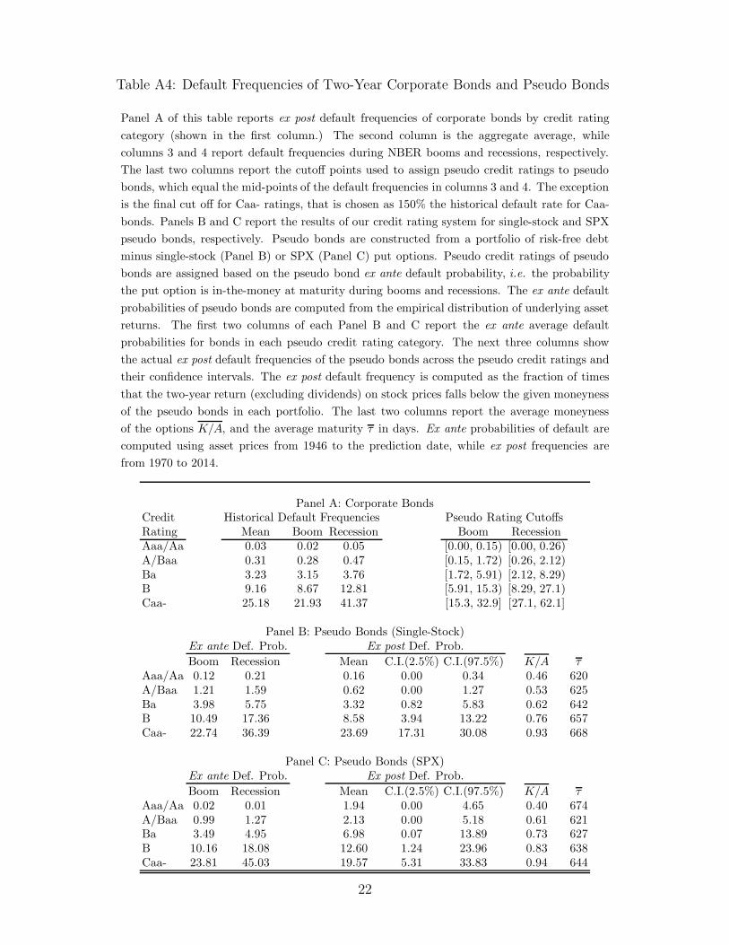
Table A4: Default Frequencies of Two-Year Corporate Bonds and Pseudo Bonds

Panel A of this table reports ex post default frequencies of corporate bonds by credit rating

category (shown in the first column.) The second column is the aggregate average, while

columns 3 and 4 report default frequencies during NBER booms and recessions, respectively.

The last two columns report the cutoff points used to assign pseudo credit ratings to pseudo

bonds, which equal the mid-points of the default frequencies in columns 3 and 4. The exception

is the final cut off for Caa- ratings, that is chosen as 150% the historical default rate for Caa-

bonds. Panels B and C report the results of our credit rating system for single-stock and SPX

pseudo bonds, respectively. Pseudo bonds are constructed from a portfolio of risk-free debt

minus single-stock (Panel B) or SPX (Panel C) put options. Pseudo credit ratings of pseudo

bonds are assigned based on the pseudo bond ex ante default probability, i.e. the probability

the put option is in-the-money at maturity during booms and recessions. The ex ante default

probabilities of pseudo bonds are computed from the empirical distribution of underlying asset

returns. The first two columns of each Panel B and C report the ex ante average default

probabilities for bonds in each pseudo credit rating category. The next three columns show

the actual ex post default frequencies of the pseudo bonds across the pseudo credit ratings and

their confidence intervals. The ex post default frequency is computed as the fraction of times

that the two-year return (excluding dividends) on stock prices falls below the given moneyness

of the pseudo bonds in each portfolio. The last two columns report the average moneyness

of the options K/A, and the average maturity τ in days. Ex ante probabilities of default are

computed using asset prices from 1946 to the prediction date, while ex post frequencies are

from 1970 to 2014.

Panel A: Corporate BondsCredit Historical Default Frequencies Pseudo Rating CutoffsRating Mean Boom Recession Boom RecessionAaa/Aa 0.03 0.02 0.05 [0.00, 0.15) [0.00, 0.26)A/Baa 0.31 0.28 0.47 [0.15, 1.72) [0.26, 2.12)Ba 3.23 3.15 3.76 [1.72, 5.91) [2.12, 8.29)B 9.16 8.67 12.81 [5.91, 15.3) [8.29, 27.1)Caa- 25.18 21.93 41.37 [15.3, 32.9] [27.1, 62.1]

Panel B: Pseudo Bonds (Single-Stock)Ex ante Def. Prob. Ex post Def. Prob.

Boom Recession Mean C.I.(2.5%) C.I.(97.5%) K/A τAaa/Aa 0.12 0.21 0.16 0.00 0.34 0.46 620A/Baa 1.21 1.59 0.62 0.00 1.27 0.53 625Ba 3.98 5.75 3.32 0.82 5.83 0.62 642B 10.49 17.36 8.58 3.94 13.22 0.76 657Caa- 22.74 36.39 23.69 17.31 30.08 0.93 668

Panel C: Pseudo Bonds (SPX)Ex ante Def. Prob. Ex post Def. Prob.

Boom Recession Mean C.I.(2.5%) C.I.(97.5%) K/A τAaa/Aa 0.02 0.01 1.94 0.00 4.65 0.40 674A/Baa 0.99 1.27 2.13 0.00 5.18 0.61 621Ba 3.49 4.95 6.98 0.07 13.89 0.73 627B 10.16 18.08 12.60 1.24 23.96 0.83 638Caa- 23.81 45.03 19.57 5.31 33.83 0.94 644

22

Table A5: Corporate LGDs: 1982 - 2013The average corporate recovery rate for senior unsecured bonds, based on rating2 years before the default. As Aaa-rated bonds have a few defaults, the recoveryrate for Aaa/Aa is based on Aa bonds. The recovery rate of A/Baa is theaverage between A and Baa. The recovery rate in booms is 1.05 multipliedby the average, while the recovery rate in recessions is 0.73 multiplied by theaverage.

Recovery rates for Corporate Bonds LGDs for Corporate BondsAverage Boom Recession Average Boom Recession

Aaa/Aa 0.39 0.41 0.28 0.61 0.59 0.72A/Baa 0.42 0.44 0.31 0.58 0.56 0.69

Ba 0.44 0.46 0.32 0.56 0.54 0.68B 0.37 0.39 0.27 0.63 0.61 0.73

Caa- 0.37 0.39 0.27 0.63 0.61 0.73

23

Table A6: The Impact of Levered Equity on Pseudo Firm Credit Spreads in Merton Model: Low Asset Volatility

This table reports the results of the following experiment. Start with a “Merton firm” with log-normally distributed assets financed by zero-coupon debt,

with face value K and maturity T , and equity. Equity is a call option on the firm. We create a pseudo firm from the equity of the “Merton firm” as its

assets whose pseudo debt has mauturity τ = 2 < T , as is in our data. We consider three values of maturity of Merton firm maturity T (10, 5, and 2.5)

and two values of asset volatility (σV = 10% and σV = 20%). In each panel, we report the corporate quantities from the data – if available – the empirical

quantities for pseudo firms in the data, and finally the theoretical implications from the experiment. For these, we report the simulation results for the

underlying Merton firm with debt maturity T , another equivalent Merton firm with debt maturity τ = two-years with otherwise the same fundamentals

except that its leverage is adjusted to match the two-year default probability in the first column, and finally the “theoretical” two-year pseudo firm built

on the theoretical T -year Merton firm’s equity. To be conservative and avoid adding more parameters, we match Merton firms’ risk-neutral probabilities

to the true default frequencies in the first column. Panel A reports credit spreads, Panel B and C the skewness and excess kurtosis of leveraged equity,

and Panel D the loss-given-default (LGDs).Panel A: Credit Spreads (bps)

Data T = 10, σV = .1 T = 5, σV = .1 T = 2.5, σV = .1Credit Def. Corporate Pseudo Pseudo Merton Merton Pseudo Merton Merton Pseudo Merton Merton Pseudo

Ratings Prob. Single-Stock SPX (T) (2) (T) (2) (T) (2)

Aaa/Aa 0.03 71.00 68.00 42.00 0.13 0.06 0.14 0.09 0.05 0.17 0.06 0.06 0.43Baa/A 0.31 121.00 171.00 119.00 1.58 0.64 1.87 1.07 0.60 3.15 0.74 0.64 6.83

Ba 3.23 293.00 308.00 209.00 22.01 8.46 33.14 14.69 8.31 47.07 9.90 8.65 88.18B 9.16 512.00 514.00 325.00 73.82 28.38 129.28 49.72 28.36 174.03 33.09 29.03 286.65

Caa+ 25.18 956.00 862.00 496.00 242.23 100.14 555.36 171.12 99.45 671.17 115.94 101.31 975.71

Panel B: Skewness of Equity ReturnsCredit Def. Corporate Pseudo Pseudo Merton Merton Pseudo Merton Merton Pseudo Merton Merton Pseudo


Aaa/Aa 0.03 -0.11 -0.31 0.00 0.00 -0.06 0.00 0.01 -0.11 0.00 -0.01 -0.59Baa/A 0.31 -0.11 -0.31 0.00 0.00 -0.10 0.00 0.01 -0.19 0.00 -0.01 -1.86

Ba 3.23 -0.11 -0.31 0.00 0.00 -0.16 0.00 0.01 -0.34 0.00 -0.01 -3.77B 9.16 -0.11 -0.31 0.00 0.00 -0.17 0.00 0.01 -0.39 0.00 -0.01 -3.71

Caa+ 25.18 -0.11 -0.31 0.00 0.00 -0.16 0.00 0.01 -0.39 0.00 -0.01 -3.01

Panel C: Kurtosis of Equity ReturnsCredit Def. Corporate Pseudo Pseudo Merton Merton Pseudo Merton Merton Pseudo Merton Merton Pseudo


Aaa/Aa 0.03 -0.19 -0.34 -0.01 -0.01 0.12 0.00 -0.01 0.39 0.01 0.02 6.73Baa/A 0.31 -0.19 -0.34 -0.01 -0.01 0.27 0.00 -0.01 0.97 0.01 0.02 29.92

Ba 3.23 -0.19 -0.34 -0.01 -0.01 0.56 0.00 -0.01 1.96 0.01 0.02 48.43B 9.16 -0.19 -0.34 -0.01 -0.01 0.59 0.00 -0.01 2.05 0.01 0.02 35.20

Caa+ 25.18 -0.19 -0.34 -0.01 -0.01 0.44 0.00 -0.01 1.60 0.01 0.02 18.93

Panel D: Loss-Given-Default (LGD)Credit Def. Corporate Pseudo Pseudo Merton Merton Pseudo Merton Merton Pseudo Merton Merton Pseudo


Aaa/Aa 0.03 61.00 49.60 10.20 8.15 2.45 9.71 5.35 1.87 11.34 3.29 1.75 28.38Baa/A 0.31 57.00 44.70 10.20 10.07 2.75 11.80 7.12 2.86 20.07 4.61 2.74 42.39

Ba 3.23 59.00 32.10 14.90 14.36 4.10 20.35 9.33 4.07 28.90 6.05 4.09 53.03B 9.16 56.00 27.30 15.10 18.68 5.19 27.84 11.48 5.23 37.14 7.18 5.22 60.06

Caa+ 25.18 63.00 25.00 18.00 28.15 7.25 41.71 15.95 7.23 49.67 9.28 7.25 69.69

24

Table A7: The Impact of Levered Equity on Pseudo Firm Credit Spreads in Merton Model: High Asset VolatilityThis table reports the results of the following experiment. Start with a “Merton firm” with log-normally distributed assets financed by zero-coupon debt,with face value K and maturity T , and equity. Equity is a call option on the firm. We create a pseudo firm from the equity of the “Merton firm” as itsassets whose pseudo debt has mauturity τ = 2 < T , as is in our data. We consider three values of maturity of Merton firm maturity T (10, 5, and 2.5)and two values of asset volatility (σV = 10% and σV = 20%). In each panel, we report the corporate quantities from the data – if available – the empiricalquantities for pseudo firms in the data, and finally the theoretical implications from the experiment. For these, we report the simulation results for theunderlying Merton firm with debt maturity T , another equivalent Merton firm with debt maturity τ = two-years with otherwise the same fundamentalsexcept that its leverage is adjusted to match the two-year default probability in the first column, and finally the “theoretical” two-year pseudo firm builton the theoretical T -year Merton firm’s equity. To be conservative and avoid adding more parameters, we match Merton firms’ risk-neutral probabilitiesto the true default frequencies in the first column. Panel A reports credit spreads, Panel B and C the skewness and excess kurtosis of leveraged equity,and Panel D the loss-given-default (LGDs).

Panel A: Credit SpreadsData T = 10, σV = .2 T = 5, σV = .2 T = 2.5, σV = .2

Credit Def. Corporate Pseudo Pseudo Merton Merton Pseudo Merton Merton Pseudo Merton Merton PseudoRatings Prob. Single-Stock SPX (T) (2) (T) (2) (T) (2)

Aaa/Aa 0.03 71.00 68.00 42.00 0.24 0.09 0.17 0.17 0.09 0.25 0.12 0.11 0.57Baa/A 0.31 121.00 171.00 119.00 2.90 1.21 2.17 2.03 1.29 3.30 1.41 1.25 6.67

Ba 3.23 293.00 308.00 209.00 39.35 16.46 35.47 27.20 16.55 48.10 18.57 16.10 88.21B 9.16 512.00 514.00 325.00 130.79 54.40 133.81 91.20 54.60 174.74 62.02 54.51 286.40

Caa+ 25.18 956.00 862.00 496.00 432.36 190.23 559.47 312.81 188.93 673.63 216.15 190.30 972.78

Panel B: Skewness of Equity ReturnsCredit Def. Corporate Pseudo Pseudo Merton Merton Pseudo Merton Merton Pseudo Merton Merton Pseudo


Aaa/Aa 0.03 -0.11 -0.31 0.00 0.01 -0.02 0.01 0.00 -0.07 -0.02 -0.01 -0.38Baa/A 0.31 -0.11 -0.31 0.00 0.01 -0.05 0.01 0.00 -0.13 -0.02 -0.01 -1.34

Ba 3.23 -0.11 -0.31 0.00 0.01 -0.11 0.01 0.00 -0.28 -0.02 -0.01 -3.25B 9.16 -0.11 -0.31 0.00 0.01 -0.13 0.01 0.00 -0.35 -0.02 -0.01 -3.40

Caa+ 25.18 -0.11 -0.31 0.00 0.01 -0.14 0.01 0.00 -0.37 -0.02 -0.01 -2.88

Panel C: Kurtosis of Equity ReturnsCredit Def. Corporate Pseudo Pseudo Merton Merton Pseudo Merton Merton Pseudo Merton Merton Pseudo


Aaa/Aa 0.03 -0.19 -0.34 0.01 0.00 0.03 -0.01 0.02 0.18 -0.01 -0.01 4.22Baa/A 0.31 -0.19 -0.34 0.01 0.00 0.10 -0.01 0.02 0.50 -0.01 -0.01 20.46

Ba 3.23 -0.19 -0.34 0.01 0.00 0.33 -0.01 0.02 1.35 -0.01 -0.01 40.15B 9.16 -0.19 -0.34 0.01 0.00 0.43 -0.01 0.02 1.64 -0.01 -0.01 31.20

Caa+ 25.18 -0.19 -0.34 0.01 0.00 0.38 -0.01 0.02 1.46 -0.01 -0.01 17.54

Panel D: Loss-Given-Default (LGD)Credit Def. Corporate Pseudo Pseudo Merton Merton Pseudo Merton Merton Pseudo Merton Merton Pseudo


Aaa/Aa 0.03 61 49.6 10.2 15.86 2.84 11.72 11.98 2.53 15.97 7.55 2.55 35.22Baa/A 0.31 57 44.7 10.2 18.74 3.67 13.68 13.20 3.72 20.78 8.56 3.42 41.83

Ba 3.23 59 32.1 14.9 25.38 5.95 21.79 17.01 5.81 29.53 11.47 5.83 53.71B 9.16 56 27.3 15.1 32.15 7.94 28.82 20.72 7.88 37.35 13.62 7.96 60.41

Caa+ 25.18 63 25 18 45.84 12.03 42.03 28.03 11.90 49.99 17.27 12.02 69.93

25

Table A8: Firm-by-Firm Matched Comparison of Pseudo Spreads, Corporate Bond Spreads,and CDS Spreads.This table contains the firm-by-firm comparison of pseudo bonds, corporate bonds, and credit default swaps.We consider firms in the S&P500 – to ensure highly liquid underlying options – and in the CDX index –to ensure high liquid underlying corporate bonds. For each firm in the intersection of these portfolios, weconstruct a pseudo firm from its equity so as to match its credit rating. We report the average pseudospreads, corporate bond spreads, and CDS spreads for this (small) set of firms. We are not able to fill datafor Aaa/Aa, because it requires extreme OTM options that are not available for this set of firm highly ratedfirms.

Pseudo Credit Spreads Corporate Bonds Credit Default SwapsAvgSp Boom Recess AvgSp Boom Recess AvgSp Boom Recess

Aaa/Aa - - - - - - - - -A/Baa 146 139 201 136 114 295 59 54 101

Ba 317 311 404 349 340 455 283 273 411B 514 493 717 414 394 594 372 359 501

Caa- - - - - - - - - -

Table A9: Pseudo Spreads and Future Economic Growth

This table reports the results of the following predictive regression:

∆hYt+h = α +

p∑

i=1

βi∆Yt−i + γ1 Pseudo Spreadt + γ2 GZ Spreadt + Controlst + εt+h

where ∆h is the “h-period” lag operator, Pseudo Spreadt is the option-based pseudo spread

index, GZ Spreadt is Gilchrist Zakrajsek (2012) spread, or its orthogonal component to the

Pseudo Spreadt when the latter is in the same regression, and “Controls” include the term

spread, the real Federal Funds rate, and the option-implied “fear gauge” VIX. The number

of lags p is determined by the Akaike Information Criterion. The pseudo spread is computed

separately for SPX pseudo bonds and single-stock pseudo bonds, and for each case reflects the

equally weighted average of HY and IG spreads with 6-months, 1-year, and 2-year maturities

(6 series). The prediction horizon is either h = 3 months or h = 12 months. The predicted

economic variables are in the title of each panel. Frequency is monthly except for Panel D, where

it is quarterly. All regression coefficients are multiplied by 100. Hodrick-adjusted t-statistics

are in parenthesis.

26

Panel A: Single Stocks Pseudo Spreads (January 1996 to June 2015)

A1: Payroll Growthh = 3 months h= 12 months

Pseudo Spread -0.18 -0.22 -0.19 -0.28 -0.78 -0.91 -1.11 -1.51t-stat -3.05 -2.91 -3.13 -3.47 -4.32 -4.87 -4.32 -5.28GZ Spread -0.28 -0.19 -0.33 -0.24 -1.11 -0.57 -1.66 -1.05t-stat -2.79 -1.71 -3.33 -2.26 -5.06 -3.20 -5.80 -5.27Term Spread 0.05 -0.02 -0.01 0.13 -0.11 -0.11t-stat 0.86 -0.37 -0.25 1.01 -0.83 -0.84Real FFR 0.01 -0.03 -0.02 -0.09 -0.26 -0.25t-stat 0.46 -1.06 -0.92 -1.17 -3.13 -2.98VIX 0.00 0.01 0.01 0.08 0.08 0.11t-stat 0.54 1.17 1.52 3.41 4.47 4.47R2 0.80 0.82 0.83 0.81 0.83 0.84 0.64 0.63 0.66 0.71 0.70 0.77

A2: Unemployment Rate ChangePseudo Spread 13.26 15.36 14.41 21.29 51.38 52.94 75.48 97.03t-stat 2.70 2.73 2.74 3.45 3.97 3.95 3.97 4.58GZ Spread 17.81 11.58 24.78 20.11 51.14 8.85 98.06 61.30t-stat 2.64 1.66 3.62 2.81 3.62 0.60 4.85 3.62Term Spread -5.29 -0.53 -0.52 -11.89 -0.77 1.45t-stat -1.01 -0.11 -0.10 -0.74 -0.05 0.09Real FFR -0.40 4.10 3.80 11.07 25.34 23.86t-stat -0.14 1.48 1.38 1.26 2.58 2.44VIX -0.23 -0.52 -0.82 -4.79 -4.23 -6.73t-stat -0.35 -1.00 -1.33 -2.54 -2.75 -3.31R2 0.50 0.51 0.53 0.51 0.57 0.58 0.46 0.37 0.46 0.60 0.59 0.67

A3: Industrial Production GrowthPseudo Spread -0.76 -0.89 -0.99 -1.37 -2.59 -2.61 -4.40 -5.48t-stat -3.62 -3.68 -3.70 -4.53 -3.78 -3.95 -3.98 -4.55GZ Spread -0.97 -0.52 -1.29 -0.85 -2.10 -0.10 -4.25 -2.34t-stat -3.44 -1.72 -4.49 -3.03 -3.58 -0.15 -4.65 -3.11Term Spread 0.39 0.35 0.31 1.20 1.26 0.93t-stat 1.94 1.80 1.58 1.91 1.97 1.46Real FFR 0.19 0.09 0.09 0.32 -0.06 -0.05t-stat 1.76 0.88 0.88 0.92 -0.16 -0.15VIX 0.04 0.04 0.07 0.34 0.27 0.46t-stat 1.16 1.47 2.28 3.31 3.49 4.06R2 0.55 0.54 0.58 0.59 0.57 0.64 0.30 0.19 0.29 0.45 0.30 0.49

A4: GDP GrowthPseudo Spread -0.21 -0.22 -0.44 -0.54 -0.52 -0.48 -1.38 -1.63t-stat -1.86 -2.08 -2.13 -2.62 -2.07 -2.01 -3.26 -3.45GZ Spread -0.16 -0.02 -0.39 -0.20 -0.28 0.17 -1.14 -0.54t-stat -1.89 -0.12 -2.68 -1.31 -1.19 0.46 -2.88 -1.39Term Spread 0.14 0.12 0.11 0.68 0.63 0.61t-stat 1.24 1.12 1.06 1.98 1.73 1.68Real FFR 0.08 0.03 0.04 0.30 0.15 0.20t-stat 1.28 0.44 0.80 1.84 0.79 1.13VIX 0.04 0.03 0.05 0.14 0.12 0.17t-stat 1.75 2.23 2.34 2.75 2.46 2.93R2 0.20 0.16 0.18 0.29 0.22 0.31 0.14 0.10 0.13 0.35 0.24 0.36

27

Table A9: (cntd.) Pseudo Spreads and Future Economic Growth

Panel B: SPX Pseudo Spreads (January 1990 to June 2015)

B1: Payroll Growthh = 3 months h= 12 months

Pseudo Spread -0.12 -0.14 -0.16 -0.25 -0.56 -0.67 -0.99 -1.48t-stat -2.82 -2.66 -2.49 -3.11 -3.94 -4.13 -3.11 -3.73GZ Spread -0.16 -0.11 -0.17 -0.16 -0.77 -0.54 -1.02 -0.91t-stat -2.24 -1.49 -2.18 -1.96 -4.10 -3.09 -4.10 -3.96Term Spread 0.05 0.00 -0.01 0.29 0.08 -0.05t-stat 1.40 0.10 -0.14 2.64 0.66 -0.40Real FFR 0.00 -0.03 -0.04 -0.06 -0.22 -0.29t-stat 0.09 -1.27 -1.85 -0.90 -2.85 -3.62VIX 0.01 0.00 0.02 0.08 0.03 0.13t-stat 0.65 -0.12 1.57 2.33 2.02 3.11R2 0.74 0.75 0.76 0.75 0.76 0.78 0.54 0.56 0.57 0.61 0.63 0.68

B2: Unemployment Rate ChangePseudo Spread 9.71 10.59 12.97 21.10 34.32 36.32 72.65 106.34t-stat 2.51 2.48 2.26 2.96 3.14 3.11 3.06 3.67GZ Spread 11.24 7.36 16.00 14.79 34.58 17.44 68.97 61.77t-stat 2.18 1.45 2.71 2.54 2.67 1.36 3.77 3.58Term Spread -3.39 0.67 2.55 -13.51 0.25 10.91t-stat -0.83 0.16 0.59 -0.96 0.02 0.72Real FFR 0.91 4.35 5.50 11.82 24.83 31.33t-stat 0.39 1.73 2.12 1.50 2.62 3.22VIX -0.54 -0.17 -1.40 -6.10 -2.50 -9.74t-stat -0.65 -0.36 -1.67 -2.18 -1.71 -2.99R2 0.42 0.42 0.44 0.44 0.47 0.50 0.33 0.32 0.34 0.48 0.51 0.59

B3: Industrial Production GrowthPseudo Spread -0.52 -0.62 -0.84 -1.37 -1.62 -1.84 -4.33 -6.23t-stat -3.28 -3.43 -2.62 -3.55 -3.09 -3.33 -3.00 -3.49GZ Spread -0.70 -0.51 -0.82 -0.79 -2.00 -1.34 -3.14 -2.97t-stat -3.23 -2.25 -3.27 -3.20 -3.53 -2.41 -3.70 -3.63Term Spread 0.32 0.22 0.11 1.36 1.07 0.48t-stat 2.00 1.44 0.67 2.51 1.87 0.82Real FFR 0.12 0.00 -0.07 0.32 -0.09 -0.46t-stat 1.27 0.01 -0.79 1.03 -0.25 -1.22VIX 0.05 0.01 0.11 0.43 0.15 0.64t-stat 1.12 0.54 2.24 2.59 2.21 3.20R2 0.39 0.42 0.43 0.42 0.43 0.48 0.18 0.19 0.21 0.31 0.27 0.41

B4: GDP GrowthPseudo Spread -0.10 -0.12 -0.39 -0.52 -0.38 -0.41 -1.66 -2.11t-stat -1.23 -1.44 -1.20 -1.48 -1.60 -1.84 -2.41 -2.75GZ Spread -0.13 -0.10 -0.23 -0.21 -0.44 -0.30 -0.79 -0.69t-stat -1.93 -1.01 -1.94 -1.87 -2.32 -1.09 -2.26 -2.03Term Spread 0.11 0.10 0.04 0.68 0.71 0.47t-stat 1.11 1.22 0.43 2.15 2.01 1.38Real FFR 0.04 0.02 -0.02 0.26 0.22 0.07t-stat 0.64 0.35 -0.28 1.60 1.18 0.34VIX 0.05 0.02 0.06 0.21 0.07 0.26t-stat 1.10 1.33 1.38 2.34 1.53 2.65R2 0.13 0.13 0.13 0.17 0.14 0.19 0.09 0.10 0.09 0.29 0.19 0.3228

Table A10: Pseudo Spread and Future Economic Growth: Subsample ending on 6/2005

See description of Table A9 for details.

Panel A: Single Stocks Pseudo Spreads (January 1996 to June 2005)


Pseudo Spread -0.17 -0.19 -0.19 -0.23 -0.74 -0.94 -0.80 -1.19t-stat -3.29 -3.61 -2.92 -3.52 -5.56 -5.76 -5.52 -5.89GZ Spread -0.20 -0.10 -0.22 -0.12 -1.18 -0.96 -1.43 -1.20t-stat -3.14 -1.00 -2.78 -1.12 -5.26 -3.62 -5.28 -4.13Term Spread 0.08 -0.01 0.02 0.55 -0.52 -0.36t-stat 0.82 -0.08 0.24 1.32 -1.38 -0.96Real FFR 0.02 -0.02 -0.01 0.12 -0.47 -0.37t-stat 0.31 -0.44 -0.14 0.60 -2.24 -1.82VIX 0.01 0.00 0.01 0.04 0.05 0.06t-stat 0.97 0.71 1.42 2.08 2.18 2.78R2 0.81 0.79 0.82 0.82 0.79 0.84 0.72 0.82 0.83 0.76 0.88 0.90

A2: Unemployment Rate ChangePseudo Spread 13.73 14.11 13.76 14.98 43.48 45.49 51.66 61.81t-stat 2.72 2.75 2.26 2.42 3.82 3.79 3.46 3.47GZ Spread 12.03 4.30 12.19 5.71 47.10 32.42 72.85 61.55t-stat 2.20 0.62 2.05 0.83 2.93 1.71 3.23 2.76Term Spread -7.30 -4.35 -5.26 -35.23 16.27 8.55t-stat -0.71 -0.43 -0.52 -1.03 0.53 0.28Real FFR -2.71 -0.10 -1.08 -10.66 28.01 22.48t-stat -0.50 -0.02 -0.20 -0.57 1.54 1.31VIX -0.10 0.10 -0.29 -2.60 -2.61 -3.49t-stat -0.14 0.16 -0.41 -1.50 -1.43 -1.80R2 0.34 0.26 0.35 0.34 0.28 0.35 0.40 0.46 0.50 0.48 0.73 0.75

A3: Industrial Production GrowthPseudo Spread -0.57 -0.67 -0.65 -0.89 -1.89 -2.41 -2.07 -3.23t-stat -3.01 -3.29 -2.77 -3.47 -4.32 -4.67 -3.91 -4.27GZ Spread -0.77 -0.61 -0.99 -0.84 -3.26 -3.12 -4.56 -4.53t-stat -2.94 -1.90 -3.26 -2.40 -4.33 -3.45 -4.32 -4.14Term Spread 0.59 0.48 0.49 3.33 1.14 1.16t-stat 1.52 1.25 1.28 2.05 0.70 0.74Real FFR 0.27 0.10 0.12 1.53 -0.29 -0.28t-stat 1.31 0.47 0.57 1.75 -0.31 -0.32VIX 0.02 0.03 0.05 0.08 0.18 0.18t-stat 0.61 1.36 1.71 1.03 2.02 2.04R2 0.43 0.50 0.52 0.45 0.56 0.58 0.31 0.56 0.55 0.35 0.75 0.75

A4: GDP GrowthPseudo Spread -0.19 -0.21 -0.31 -0.39 -0.77 -0.84 -1.34 -1.60t-stat -1.30 -1.38 -1.58 -1.83 -2.33 -2.43 -2.84 -2.93GZ Spread -0.20 -0.16 -0.39 -0.34 -0.80 -0.64 -1.65 -1.44t-stat -1.43 -0.96 -1.83 -1.36 -2.43 -1.73 -2.90 -2.52Term Spread -0.10 -0.17 -0.16 0.85 -0.67 -0.39t-stat -0.42 -0.77 -0.71 0.65 -0.49 -0.29Real FFR -0.07 -0.17 -0.15 0.35 -0.74 -0.55t-stat -0.68 -1.59 -1.43 0.55 -1.03 -0.81VIX 0.03 0.04 0.04 0.14 0.15 0.16t-stat 1.68 2.16 2.21 2.60 2.55 2.71R2 0.15 0.18 0.16 0.13 0.23 0.22 0.19 0.25 0.24 0.30 0.56 0.56

29

Table A10: (cntd.) Pseudo Spread and Future Economic Growth: Subsample ending on6/2005

Panel B: SPX Pseudo Spreads (January 1990 to June 2005)


Pseudo Spread -0.08 -0.09 -0.09 -0.14 -0.41 -0.46 -0.22 -0.63t-stat -2.38 -2.53 -1.23 -1.89 -3.82 -4.14 -1.18 -3.18GZ Spread -0.10 -0.06 -0.09 -0.10 -0.67 -0.55 -0.74 -0.76t-stat -1.87 -1.03 -1.34 -1.46 -3.61 -2.61 -2.92 -3.03Term Spread 0.05 0.03 0.00 0.46 -0.02 -0.12t-stat 0.74 0.43 0.06 1.66 -0.08 -0.41Real FFR 0.00 -0.02 -0.04 0.05 -0.29 -0.34t-stat -0.05 -0.47 -0.81 0.30 -1.46 -1.79VIX 0.00 0.00 0.01 0.00 0.02 0.05t-stat 0.46 0.04 1.21 -0.17 0.80 1.88R2 0.68 0.67 0.69 0.69 0.69 0.71 0.52 0.56 0.58 0.57 0.65 0.66

B2: Unemployment Rate ChangePseudo Spread 6.34 6.46 3.36 6.15 21.70 22.34 5.04 24.86t-stat 2.12 2.13 0.64 1.01 2.05 2.08 0.28 1.21GZ Spread 6.04 3.54 4.82 5.10 26.92 20.06 35.27 35.95t-stat 1.47 0.80 0.93 0.97 1.78 1.24 1.77 1.79Term Spread -6.39 -5.08 -3.80 -41.68 -16.09 -12.68t-stat -0.86 -0.66 -0.49 -1.53 -0.58 -0.47Real FFR -1.75 -0.42 0.30 -8.18 10.76 12.66t-stat -0.43 -0.09 0.07 -0.52 0.62 0.75VIX 0.25 0.27 -0.20 0.78 -1.11 -2.22t-stat 0.32 0.50 -0.23 0.30 -0.59 -0.77R2 0.22 0.20 0.22 0.23 0.24 0.24 0.22 0.23 0.25 0.37 0.46 0.46

B3: Industrial Production GrowthPseudo Spread -0.36 -0.38 -0.36 -0.74 -1.14 -1.25 -0.46 -2.13t-stat -2.68 -2.88 -1.34 -2.70 -2.54 -2.74 -0.59 -2.46GZ Spread -0.53 -0.43 -0.59 -0.63 -2.16 -1.96 -2.78 -2.86t-stat -3.00 -1.98 -2.30 -2.52 -3.46 -2.80 -3.16 -3.26Term Spread 0.20 0.05 -0.07 0.59 -1.00 -1.19t-stat 0.63 0.16 -0.22 0.55 -0.88 -1.08Real FFR 0.08 -0.07 -0.14 0.06 -1.20 -1.32t-stat 0.46 -0.40 -0.78 0.10 -1.62 -1.83VIX 0.00 0.01 0.06 -0.09 0.06 0.17t-stat 0.12 0.22 1.69 -0.77 0.66 1.33R2 0.20 0.24 0.26 0.19 0.25 0.28 0.15 0.30 0.31 0.17 0.39 0.40

B4: GDP GrowthPseudo Spread -0.04 -0.04 -0.11 -0.24 -0.24 -0.25 -0.80 -1.44t-stat -0.44 -0.46 -0.53 -1.13 -0.78 -0.80 -1.34 -2.20GZ Spread -0.07 -0.07 -0.19 -0.20 -0.39 -0.35 -0.88 -0.98t-stat -0.70 -0.55 -1.31 -1.43 -1.34 -1.03 -1.96 -2.17Term Spread -0.19 -0.24 -0.28 -0.40 -0.85 -1.16t-stat -1.04 -1.41 -1.52 -0.59 -1.06 -1.55Real FFR -0.13 -0.19 -0.21 -0.32 -0.70 -0.89t-stat -1.42 -2.01 -2.03 -0.90 -1.50 -2.02VIX 0.01 0.01 0.03 0.09 0.06 0.19t-stat 0.44 1.07 1.20 1.19 1.26 2.20R2 0.08 0.09 0.07 0.06 0.09 0.08 0.03 0.06 0.05 0.03 0.11 0.19

30

Table A11: Pseudo Spread and Future Economic Growth: Subsample 7/2005 - 6/2015

See description of Table A9 for details.

Panel A: Single Stocks Pseudo Spreads (July 2005 to June 2015)


Pseudo Spread -0.17 -0.25 -0.15 -0.33 -0.80 -0.78 -1.18 -1.65t-stat -2.31 -2.14 -1.69 -2.26 -3.49 -3.49 -2.94 -3.38GZ Spread -0.32 -0.30 -0.44 -0.47 -1.04 0.05 -1.97 -1.15t-stat -2.16 -1.47 -2.26 -1.94 -3.49 0.20 -3.51 -3.93Term Spread 0.03 -0.11 -0.11 -0.29 -0.73 -0.61t-stat 0.34 -1.32 -1.36 -1.27 -2.62 -2.50Real FFR -0.02 -0.11 -0.12 -0.45 -0.83 -0.68t-stat -0.50 -2.20 -2.10 -2.83 -3.83 -3.99VIX -0.01 0.01 0.01 0.07 0.07 0.11t-stat -0.38 0.79 0.54 1.81 2.28 2.38R2 0.79 0.83 0.83 0.80 0.87 0.87 0.60 0.53 0.60 0.72 0.70 0.76

A2: Unemployment Rate ChangePseudo Spread 13.49 18.47 14.57 33.06 54.72 50.98 86.74 125.83t-stat 2.07 2.17 1.86 2.86 3.22 3.02 2.83 3.36GZ Spread 24.17 23.51 44.05 45.51 55.17 -18.18 137.44 89.09t-stat 2.16 1.64 2.96 2.65 2.79 -0.75 3.61 3.68Term Spread -3.77 8.23 8.42 16.50 42.91 39.35t-stat -0.47 0.97 1.00 0.58 1.45 1.36Real FFR 1.63 11.49 11.84 37.46 67.70 57.05t-stat 0.34 2.00 2.03 1.88 3.02 2.80VIX -0.06 -1.77 -1.67 -4.98 -5.12 -8.80t-stat -0.05 -1.81 -1.40 -1.46 -1.93 -2.22R2 0.55 0.62 0.61 0.56 0.73 0.73 0.46 0.36 0.46 0.66 0.66 0.72

A3: Industrial Production GrowthPseudo Spread -0.87 -0.94 -1.23 -1.85 -3.01 -2.41 -6.21 -7.54t-stat -3.01 -2.68 -2.57 -3.01 -3.09 -2.74 -3.26 -3.12GZ Spread -1.12 -0.33 -1.82 -1.18 -2.41 2.72 -6.37 -2.51t-stat -2.46 -0.54 -2.81 -1.90 -2.45 2.30 -2.89 -1.87Term Spread 0.22 0.08 0.08 -1.04 -1.35 -1.35t-stat 0.77 0.26 0.28 -0.97 -1.17 -1.17Real FFR 0.09 -0.07 0.00 -1.18 -1.82 -1.41t-stat 0.58 -0.40 0.00 -1.42 -1.86 -1.58VIX 0.06 0.07 0.13 0.55 0.36 0.69t-stat 0.92 1.40 1.84 3.05 2.69 3.06R2 0.58 0.54 0.58 0.60 0.57 0.64 0.35 0.18 0.38 0.57 0.31 0.58

A4: GDP GrowthPseudo Spread -0.34 -0.32 -0.51 -0.69 -0.92 -0.69 -1.29 -1.21t-stat -2.23 -2.47 -1.67 -1.97 -2.79 -2.37 -2.57 -2.15GZ Spread -0.23 0.10 -0.49 -0.28 -0.21 0.96 -0.46 0.13t-stat -1.84 0.37 -1.84 -1.18 -0.70 1.65 -0.97 0.28Term Spread -0.01 -0.06 -0.08 -0.43 -0.34 -0.40t-stat -0.04 -0.30 -0.36 -0.78 -0.63 -0.73Real FFR -0.04 -0.12 -0.08 -0.73 -0.81 -0.71t-stat -0.31 -0.83 -0.66 -1.31 -1.42 -1.30VIX 0.03 0.03 0.06 0.05 -0.04 0.04t-stat 0.88 0.97 1.34 0.81 -0.77 0.57R2 0.23 0.08 0.22 0.26 0.09 0.26 0.19 -0.02 0.26 0.45 0.23 0.44

31

Table A11: (cntd.) Pseudo Spread and Future Economic Growth: Subsample 7/2005 -6/2015

Panel B: SPX Pseudo Spreads (July 2005 to June 2015)


Pseudo Spread -0.19 -0.27 -0.24 -0.38 -0.79 -0.88 -1.99 -2.34t-stat -2.56 -2.19 -2.23 -2.70 -3.61 -3.53 -3.26 -3.42GZ Spread -0.32 -0.33 -0.44 -0.42 -1.04 -0.38 -1.97 -1.02t-stat -2.16 -1.38 -2.26 -1.58 -3.49 -1.21 -3.51 -2.90Term Spread 0.03 -0.11 -0.10 -0.22 -0.73 -0.53t-stat 0.40 -1.32 -1.16 -0.98 -2.62 -2.26Real FFR -0.03 -0.11 -0.11 -0.52 -0.83 -0.71t-stat -0.79 -2.20 -1.97 -3.06 -3.83 -3.84VIX 0.00 0.01 0.01 0.17 0.07 0.19t-stat 0.25 0.79 0.67 2.64 2.28 2.78R2 0.78 0.83 0.83 0.80 0.87 0.87 0.55 0.53 0.55 0.77 0.70 0.80

B2: Unemployment Rate ChangePseudo Spread 14.00 19.33 26.29 39.60 47.90 49.79 152.01 179.55t-stat 2.09 2.17 2.35 3.12 2.91 2.89 3.16 3.41GZ Spread 24.17 29.95 44.05 40.52 55.17 11.41 137.44 77.17t-stat 2.16 1.73 2.96 2.17 2.79 0.42 3.61 2.86Term Spread -4.32 8.23 7.56 10.65 42.91 32.77t-stat -0.55 0.97 0.88 0.38 1.45 1.14Real FFR 3.18 11.49 11.04 44.62 67.70 59.91t-stat 0.64 2.00 1.89 2.17 3.02 2.84VIX -1.48 -1.77 -2.31 -12.97 -5.12 -15.02t-stat -0.84 -1.81 -1.43 -2.45 -1.93 -2.68R2 0.53 0.62 0.62 0.59 0.73 0.73 0.38 0.36 0.38 0.73 0.66 0.78

B3: Industrial Production GrowthPseudo Spread -0.71 -0.92 -1.46 -2.14 -2.38 -2.01 -9.89 -11.02t-stat -2.74 -2.48 -2.27 -2.97 -2.72 -2.46 -3.15 -3.13GZ Spread -1.12 -0.96 -1.82 -1.38 -2.41 1.60 -6.37 -2.29t-stat -2.46 -1.33 -2.81 -2.00 -2.45 1.31 -2.89 -1.76Term Spread 0.36 0.08 0.16 -0.19 -1.35 -0.55t-stat 1.29 0.26 0.54 -0.20 -1.17 -0.55Real FFR 0.07 -0.07 -0.04 -1.21 -1.82 -1.41t-stat 0.42 -0.40 -0.21 -1.45 -1.86 -1.60VIX 0.10 0.07 0.16 1.05 0.36 1.15t-stat 1.03 1.40 1.70 3.09 2.69 3.11R2 0.51 0.54 0.54 0.55 0.57 0.60 0.25 0.18 0.25 0.65 0.31 0.66

B4: GDP GrowthPseudo Spread -0.24 -0.23 -0.84 -0.92 -0.67 -0.42 -2.74 -2.37t-stat -1.86 -2.08 -1.33 -1.55 -2.11 -1.50 -2.46 -2.38GZ Spread -0.23 0.05 -0.49 -0.18 -0.21 1.61 -0.46 0.83t-stat -1.84 0.13 -1.84 -0.67 -0.70 1.82 -0.97 1.36Term Spread 0.03 -0.06 -0.02 -0.36 -0.34 -0.15t-stat 0.12 -0.30 -0.11 -0.66 -0.63 -0.29Real FFR -0.07 -0.12 -0.09 -0.80 -0.81 -0.67t-stat -0.47 -0.83 -0.75 -1.38 -1.42 -1.27VIX 0.09 0.03 0.09 0.26 -0.04 0.22t-stat 1.03 0.97 1.21 2.14 -0.77 2.01R2 0.12 0.08 0.10 0.27 0.09 0.26 0.09 -0.02 0.21 0.64 0.23 0.67

32

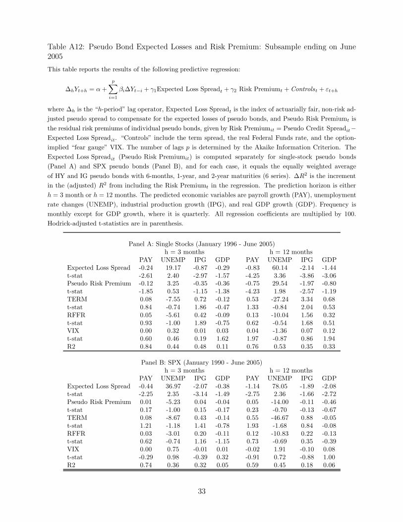
Table A12: Pseudo Bond Expected Losses and Risk Premium: Subsample ending on June2005


∆hYt+h = α +

p∑

i=1

βi∆Yt−i + γ1Expected Loss Spreadt + γ2 Risk Premiumt + Controlst + εt+h

where ∆h is the “h-period” lag operator, Expected Loss Spreadt is the index of actuarially fair, non-risk ad-

justed pseudo spread to compensate for the expected losses of pseudo bonds, and Pseudo Risk Premiumt is

the residual risk premiums of individual pseudo bonds, given by Risk Premiumit = Pseudo Credit Spreadit−Expected Loss Spreadit. “Controls” include the term spread, the real Federal Funds rate, and the option-

implied “fear gauge” VIX. The number of lags p is determined by the Akaike Information Criterion. The

Expected Loss Spreadit (Pseudo Risk Premiumit) is computed separately for single-stock pseudo bonds

(Panel A) and SPX pseudo bonds (Panel B), and for each case, it equals the equally weighted average

of HY and IG pseudo bonds with 6-months, 1-year, and 2-year maturities (6 series). ∆R2 is the increment

in the (adjusted) R2 from including the Risk Premiumt in the regression. The prediction horizon is either

h = 3 month or h = 12 months. The predicted economic variables are payroll growth (PAY), unemployment

rate changes (UNEMP), industrial production growth (IPG), and real GDP growth (GDP). Frequency is

monthly except for GDP growth, where it is quarterly. All regression coefficients are multiplied by 100.

Hodrick-adjusted t-statistics are in parenthesis.

Panel A: Single Stocks (January 1996 - June 2005)h = 3 months h = 12 months

PAY UNEMP IPG GDP PAY UNEMP IPG GDPExpected Loss Spread -0.24 19.17 -0.87 -0.29 -0.83 60.14 -2.14 -1.44t-stat -2.61 2.40 -2.97 -1.57 -4.25 3.36 -3.86 -3.06Pseudo Risk Premium -0.12 3.25 -0.35 -0.36 -0.75 29.54 -1.97 -0.80t-stat -1.85 0.53 -1.15 -1.38 -4.23 1.98 -2.57 -1.19TERM 0.08 -7.55 0.72 -0.12 0.53 -27.24 3.34 0.68t-stat 0.84 -0.74 1.86 -0.47 1.33 -0.84 2.04 0.53RFFR 0.05 -5.61 0.42 -0.09 0.13 -10.04 1.56 0.32t-stat 0.93 -1.00 1.89 -0.75 0.62 -0.54 1.68 0.51VIX 0.00 0.32 0.01 0.03 0.04 -1.36 0.07 0.12t-stat 0.60 0.46 0.19 1.62 1.97 -0.87 0.86 1.94R2 0.84 0.44 0.48 0.11 0.76 0.53 0.35 0.33

Panel B: SPX (January 1990 - June 2005)h = 3 months h = 12 months

PAY UNEMP IPG GDP PAY UNEMP IPG GDPExpected Loss Spread -0.44 36.97 -2.07 -0.38 -1.14 78.05 -1.89 -2.08t-stat -2.25 2.35 -3.14 -1.49 -2.75 2.36 -1.66 -2.72Pseudo Risk Premium 0.01 -5.23 0.04 -0.04 0.05 -14.00 -0.11 -0.46t-stat 0.17 -1.00 0.15 -0.17 0.23 -0.70 -0.13 -0.67TERM 0.08 -8.67 0.43 -0.14 0.55 -46.67 0.88 -0.05t-stat 1.21 -1.18 1.41 -0.78 1.93 -1.68 0.84 -0.08RFFR 0.03 -3.01 0.20 -0.11 0.12 -10.83 0.22 -0.13t-stat 0.62 -0.74 1.16 -1.15 0.73 -0.69 0.35 -0.39VIX 0.00 0.75 -0.01 0.01 -0.02 1.91 -0.10 0.08t-stat -0.29 0.98 -0.39 0.32 -0.91 0.72 -0.88 1.00R2 0.74 0.36 0.32 0.05 0.59 0.45 0.18 0.06

33

Table A13: Pseudo Bond Expected Losses and Risk Premium: Subsample July 2005 – June2015


∆hYt+h = α +

p∑

i=1

βi∆Yt−i + γ1Expected Loss Spreadt + γ2 Risk Premiumt + Controlst + εt+h

where ∆h is the “h-period” lag operator, Expected Loss Spreadt is the index of actuarially fair, non-risk ad-

justed pseudo spread to compensate for the expected losses of pseudo bonds, and Pseudo Risk Premiumt is

the residual risk premiums of individual pseudo bonds, given by Risk Premiumit = Pseudo Credit Spreadit−Expected Loss Spreadit. “Controls” include the term spread, the real Federal Funds rate, and the option-

implied “fear gauge” VIX. The number of lags p is determined by the Akaike Information Criterion. The

Expected Loss Spreadit (Pseudo Risk Premiumit) is computed separately for single-stock pseudo bonds

(Panel A) and SPX pseudo bonds (Panel B), and for each case, it equals the equally weighted average

of HY and IG pseudo bonds with 6-months, 1-year, and 2-year maturities (6 series). ∆R2 is the increment

in the (adjusted) R2 from including the Risk Premiumt in the regression. The prediction horizon is either

h = 3 month or h = 12 months. The predicted economic variables are payroll growth (PAY), unemployment

rate changes (UNEMP), industrial production growth (IPG), and real GDP growth (GDP). Frequency is

monthly except for GDP growth, where it is quarterly. All regression coefficients are multiplied by 100.

Hodrick-adjusted t-statistics are in parenthesis.

Panel A: Single Stocks (July 2005 - June 2015)h = 3 months h = 12 months

PAY UNEMP IPG GDP PAY UNEMP IPG GDPExpected Loss Spread -0.33 27.81 -1.15 -0.70 -1.82 141.73 -7.44 -1.49t-stat -2.45 2.55 -1.45 -1.68 -3.72 3.69 -2.88 -2.63Pseudo Risk Premium -0.07 9.12 -1.27 -0.50 -0.96 69.58 -5.72 -1.28t-stat -0.77 1.18 -3.04 -1.66 -2.53 2.36 -3.36 -2.54TERM 0.02 -4.54 0.20 -0.01 -0.27 12.63 -0.75 -0.43t-stat 0.30 -0.57 0.78 -0.02 -1.16 0.44 -0.77 -0.78RFFR -0.05 3.93 0.09 -0.05 -0.53 46.26 -1.13 -0.75t-stat -0.99 0.79 0.56 -0.37 -3.17 2.27 -1.40 -1.33VIX -0.01 0.36 0.06 0.05 0.06 -4.19 0.55 0.06t-stat -0.92 0.29 0.91 1.06 1.54 -1.24 3.05 1.07R2 0.83 0.59 0.60 0.27 0.76 0.71 0.58 0.44

Panel B: SPX (July 2005 - June 2015)h = 3 months h = 12 months

PAY UNEMP IPG GDP PAY UNEMP IPG GDPExpected Loss Spread -0.56 58.82 -1.22 -0.78 -2.24 196.07 -8.46 -1.18t-stat -2.56 2.74 -0.90 -1.23 -3.72 3.70 -2.56 -1.49Pseudo Risk Premium -0.07 10.18 -1.55 -0.87 -1.86 131.34 -10.46 -3.59t-stat -0.55 0.68 -2.34 -1.28 -2.81 2.52 -3.18 -2.46TERM 0.03 -4.80 0.33 0.02 -0.22 9.74 -0.35 -0.43t-stat 0.35 -0.60 1.24 0.10 -0.97 0.34 -0.37 -0.77RFFR -0.04 4.09 0.05 -0.07 -0.53 45.87 -1.29 -0.82t-stat -0.92 0.83 0.30 -0.47 -3.09 2.25 -1.55 -1.41VIX -0.01 -0.04 0.11 0.09 0.16 -11.24 1.09 0.31t-stat -0.54 -0.02 1.19 1.02 2.26 -1.99 3.09 2.19R2 0.82 0.62 0.55 0.25 0.77 0.74 0.65 0.72

34

Table A14: Pseudo Spreads and Future Economic Growth


∆hYt+h = α +

p∑

i=1

βi∆Yt−i + γ1 SPX Spreadt + γ2 Pseudo Spread Differencet + Controlst + εt+h

where ∆h is the “h-period” lag operator, the “Pseudo Spread Difference” is the difference in pseudo spreads

between single-stock and SPX indices. “Controls” include the term spread, the real Federal Funds rate,

and the option-implied “fear gauge” VIX. The number of lags p is determined by the Akaike Information

Criterion. The pseudo spread is computed separately for SPX pseudo bonds and single-stock pseudo bonds,

and for each case reflects the equally weighted average of HY and IG spreads with 6-months, 1-year, and

2-year maturities (6 series). The risk premium component of a pseudo spread is the difference between the

pseudo spread and spread as compensation of expected losses, the latter computed as default probability

times the loss-given default. The risk premium index is then computed as the equally weighted average

of HY and IG risk premia with 6-months, 1-year, and 2-year maturities (6 series). The prediction horizon

is either h = 3 months or h = 12 months. The predicted economic variables are payroll growth (PAY),

unemployment rate changes (UNEMP), industrial production growth (IPG), and real GDP growth (GDP).

Frequency is monthly except for Panel D, where it is quarterly. All regression coefficients are multiplied by

100. Hodrick-adjusted t-statistics are in parenthesis.

Panel A: Subsample January 1996 – June 2005h = 3 months h= 12 months

PAY UNEMP IPG GDP PAY UNEMP IPG GDPSPX Spread -0.20 14.34 -0.48 -0.30 -0.72 41.69 -1.31 -1.78t-stat -2.08 1.69 -1.48 -1.39 -3.34 1.98 -1.55 -2.52Single-Stock - SPX Spread -0.19 13.67 -0.67 -0.31 -0.82 53.26 -2.15 -1.23t-stat -2.93 2.29 -2.76 -1.43 -5.39 3.45 -3.86 -2.49TERM 0.08 -7.07 0.65 -0.10 0.59 -40.19 3.58 0.52t-stat 0.79 -0.69 1.62 -0.35 1.50 -1.25 2.33 0.44RFFR 0.01 -2.58 0.31 -0.07 0.15 -13.33 1.66 0.16t-stat 0.24 -0.48 1.43 -0.53 0.78 -0.75 2.01 0.28VIX 0.01 -0.17 0.00 0.03 0.03 -1.38 -0.02 0.20t-stat 0.72 -0.17 -0.09 0.96 1.12 -0.52 -0.14 2.39R2 0.82 0.33 0.45 0.10 0.76 0.48 0.36 0.32

Panel B: Subsample July 2005 – June 2015PAY UNEMP IPG GDP PAY UNEMP IPG GDP

SPX Spread -0.23 25.84 -1.45 -0.78 -1.92 147.97 -9.85 -2.76t-stat -2.23 2.35 -2.26 -1.23 -3.33 3.23 -3.14 -2.39Single-Stock - SPX Spread -0.06 2.98 -1.04 -0.26 -0.40 23.35 -2.88 0.08t-stat -0.49 0.28 -2.02 -1.34 -1.49 1.03 -2.68 0.15TERM 0.03 -4.05 0.25 0.00 -0.26 13.31 -0.55 -0.36t-stat 0.35 -0.51 0.90 0.01 -1.16 0.47 -0.57 -0.67RFFR -0.03 2.97 0.09 -0.06 -0.51 43.33 -1.19 -0.80t-stat -0.67 0.59 0.55 -0.39 -3.01 2.12 -1.43 -1.37VIX 0.00 -1.44 0.09 0.07 0.17 -12.58 1.02 0.27t-stat 0.22 -0.81 0.95 0.87 2.65 -2.47 3.06 2.07R2 0.80 0.59 0.60 0.28 0.78 0.74 0.69 0.63

35

Table A15: Default Frequencies of Short-Term Corporate Bonds and Pseudo Bonds

The left-hand-side of this table reports ex post default frequencies of corporate bonds with Moody’s credit ratings reported in the first

column across maturities. The mean is the aggregate average and columns 3 and 4 report default frequencies during NBER booms and

recessions, respectively. The two panels on the right-hand-side report the results of our credit rating methodology for SPX and single-stock

pseudo bonds. Pseudo bonds are constructed from a portfolio of risk-free debt minus put options on the SPX index or individual stocks.

Pseudo credit ratings of pseudo bonds are assigned based on the pseudo bonds ex ante default probabilities (i.e. the probabilities that the

put options are in the money at maturity) during booms and recession. In each subpanel, the first two columns report the ex ante average

default probabilities for pseudo bonds in booms and recessions, respectively, for each pseudo credit rating. The next three columns show

the actual ex post default frequencies of the pseudo bonds across the pseudo credit ratings, and their confidence intervals. The ex post

default frequency is computed as the fraction of times the stock return (excluding dividends) drops below the portfolio moneyness in the

sample. The last two columns collect the average leverage K/A of pseudo bonds, and their average time to maturity (days). The sample of

underlying asset price for ex post default frequency is 1970 to 2013.Corporate Bonds Pseudo Bonds (Single-Stock) Pseudo Bonds (SPX)

Ex ante Ex post Ex ante Ex post

Def. Prob. Default Frequency Def. Prob. Default Frequency

Mean Boom Bust Boom Bust Mean C.I. C.I. K/A τ Boom Bust Mean C.I. C.I. K/A τ(2.5%) (97.5%) (2.5%) (97.5%)

Target Maturity: 30 daysIG 0.00 0.00 0.01 0.00 0.00 0.37 0.00 0.90 0.77 33Ba 0.05 0.04 0.11 0.07 0.19 0.10 0.03 0.17 0.70 50 0.18 0.37 0.00 0.90 0.8 33B 0.22 0.19 0.43 0.58 1.23 0.34 0.16 0.52 0.78 50 0.32 0.82 0.56 0.00 1.20 0.86 31Caa- 1.89 1.61 3.47 1.65 3.64 1.96 1.48 2.44 0.83 50 1.55 3.52 2.41 1.09 3.73 0.91 33

Target Maturity: 91 daysIG 0.01 0.01 0.03 0.05 0.14 0.02 0.01 0.04 0.54 147 0.00 0.01 0.56 0.00 1.20 0.67 119Ba 0.19 0.16 0.38 0.27 0.63 0.29 0.10 0.48 0.61 139 0.23 0.68 0.56 0.00 1.20 0.74 108B 0.75 0.65 1.48 1.43 3.23 0.94 0.42 1.47 0.70 128 1.24 2.87 1.68 0.00 3.43 0.82 90Caa- 4.90 4.07 9.51 4.16 9.66 4.39 2.98 5.79 0.78 119 4.27 9.86 7.26 3.52 11.01 0.88 85

Target Maturity: 183 daysAaa/Aa 0.00 0.00 0.03 0.01 0.04 0.01 0.00 0.02 0.32 280 0.00 0.00 0.75 0.00 1.91 0.59 197A/Baa 0.03 0.02 0.09 0.14 0.35 0.08 0.02 0.13 0.50 233 0.15 0.25 0.94 0.00 2.46 0.68 192Ba 0.47 0.40 0.91 0.60 1.45 0.65 0.18 1.12 0.57 215 0.48 1.16 2.06 0.00 4.72 0.73 193B 1.69 1.47 3.33 2.69 6.51 1.79 0.75 2.82 0.68 195 2.35 5.83 2.25 0.00 5.13 0.80 189Caa- 8.88 7.25 17.73 7.59 18.25 7.32 4.87 9.76 0.79 182 7.63 18.34 8.24 2.56 13.92 0.87 183

Target Maturity: 365 daysAaa/Aa 0.01 0.00 0.05 0.03 0.12 0.03 0.00 0.07 0.33 372 0.00 0.05 1.14 0.00 3.01 0.47 355A/Baa 0.10 0.08 0.24 0.38 0.76 0.21 0.00 0.41 0.46 372 0.31 0.70 2.08 0.00 4.91 0.61 348Ba 1.19 1.08 1.91 1.50 3.16 1.30 0.24 2.37 0.55 361 1.37 2.37 3.22 0.00 7.45 0.71 352B 4.01 3.57 7.31 5.16 11.84 3.61 1.43 5.80 0.69 348 4.62 10.48 6.82 0.40 13.24 0.80 353Caa- 15.37 12.63 29.49 13.29 29.78 13.04 8.73 17.36 0.84 329 13.02 33.33 13.45 3.25 23.64 0.87 348

36

Table A16: Assets as Shares of Individual Firms: Equivalent European OptionsThis table contains the pseudo spreads constructed from individual stocks as presented in the paper, except

that pseudo bonds are computed from European-equivalent put options. European-equivalent put options

are obtained from volatilities reported from OptionsMetrics. Columns 2 to 4 report the Gaussian-kernel

weighted average credit spread of pseudo bonds, on average, and across booms and recessions.

Average Boom RecessionAaa/Aa 97 97 103A/Baa 214 213 224Ba 341 332 399B 559 530 764Caa- 899 840 1311

37

Table A17: Extensions: Types of Assets and Bankruptcy Costs. 1-year Pseudo Bonds.

Credit spreads and LGDs are shown for corporate bonds and for pseudo bonds with one year to

maturity. Pseudo bonds are constructed from a portfolio of risk-free debt minus put options on

the SPX index (column “SPX”), on individual stocks (column “Single Stocks”), on commodity

futures (column “Commodities”), on foreign currency (column “Currencies”), swaptions (col-

umn “Fixed Income”), or single stocks for underlying firms with negligible leverage (column

“Low Leverage”). Pseudo credit ratings of pseudo bonds are assigned based on the pseudo bond

ex ante default probability, i.e. the probability the put option is in the money at maturity.

In Panel B the LGDs are computed from the empirical distributions of asset returns. Panel

C and D report credit spreads and ex post LGDs for pseudo bonds that contain bankruptcy

costs calibrated to match corporate LGDs. In this case, pseudo bonds are constructed from a

portfolio of risk-free debt, put options and digital put options, the latter approximated from

traded put options. Corporate bonds are non-callable, level-coupon corporate bonds with times

to maturity between 0.5 and 1.5 years. LGDs for corporate bonds are from Moody’s. Sample

periods vary: SPX and single stocks – 1/1996 to 8/2014; commodities – mid 1980s to 2/2015;

foreign currencies – 1/1999 to 12/2014; swaptions – 7/2002 to 12/2014.

Credit Corporate SPX Single Commodities Currencies Currencies Fixed Un-leveredRating Stocks CME JPM Income Equity

Panel A: Credit Spreads across Types of Assets (bps)

Aaa/Aa 55 39 71 22 21 - 30 94A/Baa 114 83 112 39 53 - 68 169Ba 310 166 193 68 69 83 97 319B 597 270 424 174 119 75 138 658Caa- 1196 424 867 341 196 152 261 1194

Panel B: Ex-Post Loss-Given-Default (%)

Aaa/Aa 63.0 6.3 32.6 9.6 4.3 - 4.1 26.1A/Baa 68.0 7.2 32.8 9.6 4.2 0.1 4.1 22.5Ba 60.0 16.0 26.0 12.7 5.4 5.6 3.8 24.3B 54.0 11.7 21.0 12.0 4.8 4.6 2.2 20.9Caa- 62.0 12.5 17.6 14.0 6.1 5.1 3.5 18.3

Panel C: Credit Spreads with Bankruptcy Costs (bps)

Aaa/Aa 55 138 124 124 206 - 318 -A/Baa 114 295 244 190 675 - 665 713Ba 310 484 488 325 688 1086 762 985B 597 936 1237 859 1391 1213 1239 1990Caa- 1196 1491 2651 1733 2272 1350 2505 3506

Panel D: Ex-Post Loss-Given-Default with Bankruptcy Costs (%)

Aaa/Aa 63.0 - 50.9 - - - - 41.6A/Baa 68.0 70.0 67.1 70.9 69.3 67.0 69.3 60.3Ba 60.0 62.9 60.4 61.4 60.7 60.2 61.1 58.2B 54.0 55.4 52.8 53.0 54.3 53.9 54.3 51.4Caa- 62.0 63.6 59.8 61.8 62.5 61.7 62.1 59.1

38

Table A18: Common Factors in Pseudo Bonds of Pseudo Firms with Heterogeneous Assets

Regression result of credit spreads of pseudo bonds issued by pseudo firms with assets defined

in the first row on a pseudo credit spread factor. The credit spread factor is equal to the average

of standardized credit spreads across the asset classes in the first column. Panel A reports the

results for IG pseudo bonds, and Panel B reports results for HY pseudo bonds. The left panels

use 1-year pseudo bonds while right-hand panels use 2-year pseudo bonds. The sample periods

is from January 1996 to August 2014, except for foreign currencies (start January 1999) and

fixed income (start July 2002).

Panel A. IG Pseudo Bonds1-year 2-year

b t(b) R2 b t(b) R2

SPX 1.07 8.36 0.62 1.02 7.36 0.66single-stock 1.12 5.25 0.53 0.98 12.01 0.65commodity 1.03 6.90 0.71 0.94 3.9 0.55cme fx 0.51 2.47 0.12jpm fxfixed income 1.01 5.70 0.41 1.29 6.45 0.52

Panel B. HY Pseudo Bonds1-year 2-year

b t(b) R2 b t(b) R2

SPX 1.09 17.29 0.80 1.09 11.97 0.83single-stock 1.06 13.24 0.76 1.01 12.13 0.71commodity 0.99 14.86 0.67 0.97 13.36 0.65cme fx 0.98 10.45 0.71jpm fx 1.07 11.46 0.87 1.05 13.8 0.79fixed income 0.80 5.49 0.57 0.89 5.99 0.65

39

Option-Based Credit Spreads - Booth School of...

Documents

Transcript of Option-Based Credit Spreads - Booth School of...