Optimum Simple Step-stress Plans for Accelerated Life Testing

IEEE TRANSACTIONS ON RELIABILITY, VOL. R-32, NO. 1, APRIL 1983 59

Optimum Simple Step-Stress Plans forAccelerated Life Testing

Robert Miller, Member ASQC section 2. The test data are used to estimate the parametersGeneral Electric Co., Schenectady of the relationship. The relationship is then extrapolated to

Wayne Nelson, Senior Member IEEE & ASQC estimate life at a constant low design stress. Estimation isGeneral Electric Co., Schenectady usually done by maximum likelihood (ML) rather than

least squares since the assumed life distribution is often nots-normal but exponential or Weibull.

Key Words-Accelerated test, Step-stress, Constant-stress test, Ex-ponential life distribution, Maximum likelihood estimation. Step Stress

Reader Aids- In a time-step-stress accelerated life test, stress on eachPurpose: Widen state of the art unit is not constant but is increased by planned steps atSpecial math needed for explanations: Statistics, Maximum likelihood planned times. A test unit starts at a specified low stress. If

theory the unit does not fail in a specified time, stress on it isSpecial math needed to use results: None theuni d es f a specified time , stress isResults useful to: Engineers and accelerated test planners raised and held a specified time. Specimen stress is

repeatedly increased and held, until the specimen fails. TheAbstract-This paper presents optimum plans for simple (two step-stress pattern is chosen to assure failures quickly.

stresses) step-stress tests where all units are run to failure. Such plans As with the constant-stress test, one estimates theminimize the asymptotic variance of the maximum likelihood estimator(MLE) of the mean life at a design stress. The life-test model consists of: parameters of a model for life under step stressing. The1) an exponential life distribution with 2) a mean that is a log-linear func- parameter estimates are used to estimate life at a constanttion of stress, and 3) a cumulative exposure model for the effect of chang- design stress. However, one now needs a model that relatesing stress. Two types of simple step-stress tests are considered: 1) a time- the life distribution under step stressing to that understep test and 2) a failure-step test. A time-step test runs a specified time at constant stress. Cumulative exposure models for life underthe first stress, whereas, a failure-step test runs until a specified propor- step-stressing have been presented by [1, 8, 10, 17].tion of units fail at the first stress. New results include: 1) the optimumtime at the first stress for time-step test and 2) the optimum proportionfailing at the low stress for a failure-step test, and 3) the asymptotic Overviewvariance of these optimum tests. Both the optimum time-step and failure-step tests have the same asymptotic variance as the corresponding op- This paper considers step-stress tests using only twotimum constant-stress test. Thus step-stress tests yield the same amount of stresses. In a time-step test, units are initially placed on testinformation as constant-stress tests. at stress x, and run until time T,, when the stress is changed

to x2; and the test is continued until all units run to failure.In a failure-step test, stress is changed to x2 when a fraction

1. ACCELERATED LIFE TESTING P1 of the units fail at stress x, and the remaining fractionare run to failure. Such tests are called simple step-stress

Accelerated life testing quickly yields information on tests since they use only two stresses.product life. Test units are run at high stress and fail This paper presents optimum simple step-stress testssooner than at design stress. The short lives are then ex- employing an exponential life distribution at constanttrapolated to estimate life at design conditions. Such stress and the cumulative exposure model of [8, 10]. Whileoverstress testing reduces time and cost. Overstress in- simple, these results provide much needed insight into thevolves high temperature, voltage, pressure, vibration, design of step-stress tests. Further work is needed to extendcycling rate, load, etc., or some combination of them. results to other distributions and censored tests.Engineering experience usually suggests such accelerating Section 2 describes the accelerated test and cumulativevariables for a specific product or material. exposure models. Section 3 presents the optimum simple

time-step test. The optimum simple failure-step test isConstant Stress presented in section 4. Section 5 discusses the optimum

constant-stress test. Section 6 compares the properties ofIn a constant-stress accelerated test, units are each run the optimum test plans.

at a (possibly different) constant high stress. Life at adesign stress is estimated by regression methods as follows. NotationA relationship between life and constant stress is

assumed. For example, for voltage stress, the inverse n total sample sizepower law is often used; it is a linear relationship between XD, XH, XL, X1, X2 transformed stresses (Design, High,log mean life and log voltage. It is discussed in [6] and in Low, 1-st, 2-nd)

0018-9529/83/0400-0059$01 .00©)1983 IEEE

60 IEEE TRANSACTIONS ON RELIABILITY, VOL. R-32, NO. 1, APRIL 1983

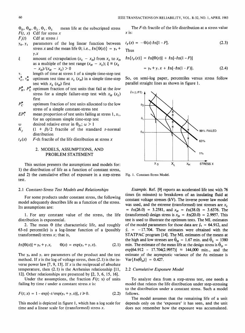
0D9 OH9'L9 01 C02 mean life at the subscripted stress The F-th fractile of the life distribution at a stress valueF(t, x) Cdf for stress x x is:Fi(t) Cdf at stress iyo, y, parameters of the log linear function between tF(X) = - e(x) ln[I -1]. (2.3)

stress x and the mean life e; i.e., In{e(x)} = Yo + Thusy'X

4 amount of extrapolation (XL - XD) from XL to XD In{tF(x)} = In[O(x)] + In[-In(l - F)]as a multiple of the test range (XH - XL); 4 (XL- XD)/(XH - XL) > 0 = yO + y, x + In[-In(I -F)]. (2.4)

T, length of time at stress 1 of a simple time-step testTL, H optimum test time atXL (xH) in a simple time-step So, on semi-log paper, percentiles versus stress follow

test with XL (XH) first parallel straight lines as shown in figure 1.PH, PL optimum fraction of test units that fail at the low

stress for a simple failure-step test with XH (XL) if (LIFE)first

Pc optimum fraction of test units allocated to the lowstress of a simple constant-stress test

EP* mean proportion of test units failing at stress 1, x',for an optimum simple time-step test L

co desired relative error in 0D; co > 1Kp (1 + f)/2 fractile of the standard s-normal \99%FAILED

distribution H

tF(X) F-th fractile of the life distribution at stress x 630

2. MODELS, ASSUMPTIONS, ANDPROBLEM STATEMENT 1/

This section presents the assumptions and models for: X D XL XH STRESS X1) the distribution of life as a function of constant stress,and 2) the cumulative effect of exposure in a step-stress Fig. 1. Constant-Stress Model.test.

2.1 Constant-Stress Test Models and Relationships Example. Ref. [9] reports an accelerated life test with 76times (in minutes) to breakdown of an insulating fluid atFor omeprouct undr cnstnt tres, te flloing constant voltage stresses (kV). The inverse power law model

model adequately describes life as a function of the stress. was used, and the extreme (transformed) test stresses are XLIts assumptions are: = In(26.0) = 3.2581, and XH = In(38.0) = 3.6376. The

1. For any constant value of the stress, the life (transformed) design stress is XD = In(20.0) = 2.9957. Thisdistribution is exponential. test is used to illustrate the optimum tests. The ML estimates

2. The mean G (the characteristic life, and roughly of the model parameters for those data are y0 = 64.912, and63-rd percentile) is a log-linear function of a (possibly Yi = - 17.704. These estimates were obtained with thetransformed) stress x; that is, STATPAC program [14]. The ML estimates of the means at

the high and low stresses are EH = 1.67 min. and 0L = 1380ln[e(x)] = yo + yix,x (x) = exp(yo + y x). (2.1) min. The estimate of the mean life at the design stress is OD =

exp[64.912 - 17.704(2.9957)] ' 144,000 min., and theThe yo and yl are parameters of the product and the test estimate of the asymptotic variance of the In estimate ismethod. If x is the log of voltage stress, then (2.1) is the in- Var{In(6D)} = 0.427.verse power law [7, 9, 13]. If x is the reciprocal of absolutetemperature, then (2.1) is the Arrhenius relationship [11, 2.2 Cumulative Exposure Model12]. Other relationships are presented by [2, 3, 6, 15, 16].

Under the assumptions, the fraction F(t; x) of units To analyze data from a step-stress test, one needs afailing by time t under a constant stress x is: model that relates the life distribution under step-stressing

to the distribution under a constant stress. Such a modelF(t; x) = 1 - exp[-t/exp(yO + y,x)], t > 0. (2.2) follows.

The model assumes that the remaining life of a unitThis model is depicted in figure 1, which has a log scale for depends only on the 'exposure' it has seen, and the unittime and a linear scale for (transformed) stress x. does not remember how the exposure was accumulated.

MILLER/NELSON: OPTIMUM SIMPLE STEP-STRESS PLANS FOR ACCELERATED LIFE TESTING 61

More precisely, if different 'large' groups of units each When step 2 starts, units have equivalent age T' whichhave a different exposure history but the same fraction would have produced the same fraction failed seen at thefailed, then survivors of all such groups have the same re- end of step 1; that is,maining life distribution. Moreover, if then held at a con- F2(T') = FI(T,) (2.6)stant stress, the survivors will continue failing according tothe life distribution for that stress but starting at the age T' = F2 [Fl (T1)]; (2.7)corresponding to the previous fraction failed.

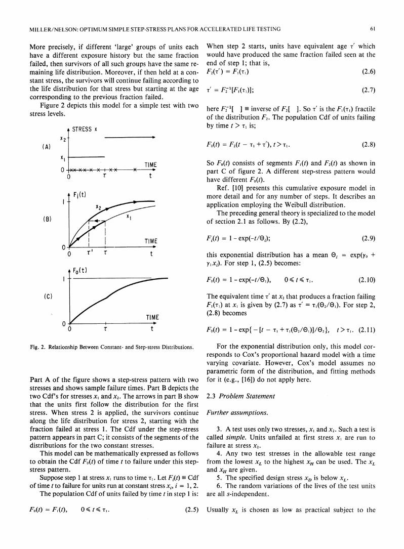
Figure 2 depicts this model for a simple test with two here FT'[ ] inverse of F2[ ]. SO T' is the Fi(T1) fractilestress levels. of the distribution F2. The population Cdf of units failing

STRESS x by time t> Ti is;X2 '

(A) F0(t) = F2(t - T1 + T'), t > Tr. (2.8)xl

TIME So Fo(t) consists of segments FI(t) and F2(t) as shown ino *(*x x x x x t part C of figure 2. A different step-stress pattern would

0 thave different Fo(t).

Ref. [10] presents this cumulative exposure model inFItj(t) more detail and for any number of steps. It describes an

application employing the Weibull distribution.X2 /The preceding general theory is specialized to the model

( B) i /<fit of section 2.1 as follows. By (2.2),

O i | |TIME Fi(t) = 1 - exp(-t/0j); (2.9)0

O T T t this exponential distribution has a mean Oi = exp(y0 +y xI). For step 1, (2.5) becomes:

i,Fo(t)Fo(t) = I - exp(-t/01), 0 ( t ( T. (2.10)

(C) The equivalent time T' at x2 that produces a fraction failingFi(T1) at xi is given by (2.7) as T- = T-(02/01). For step 2,

z i TIME (2.8) becomes

00 T t FF(t) = 1 - exp{ - [t - Ti + Ti (02/0)1/021,} t>T,. (2.11)

Fig. 2. Relationship Between Constant- and Step-stress Distributions. For the exponential distribution only, this model cor-responds to Cox's proportional hazard model with a timevarying covariate. However, Cox's model assumes noparametric form of the distribution, and fitting methods

Part A of the figure shows a step-stress pattern with two for it (e.g., [16]) do not apply here.stresses and shows sample failure times. Part B depicts thetwo Cdf's for stresses xl and x2. The arrows in part B show 2.3 Problem Statementthat the units first follow the distribution for the firststress. When stress 2 is applied, the survivors continue Further assumptions.along the life distribution for stress 2, starting with thefraction failed at stress 1. The Cdf under the step-stress 3. A test uses only two stresses, xi and x2. Such a test ispattern appears in part C; it consists of the segments of the called simple. Units unfailed at first stress xl are run todistributions for the two constant stresses. failure at stress x2.

This model can be mathematically expressed as follows 4. Any two test stresses in the allowable test rangeto obtain the Cdf Fo(t) of time t to failure under this step- from the lowest XL to the highest XH can be used. The XLstress pattern. and XH are given.

Suppose step 1 at stress x, runs to time T,. Let Fi(t) -Cdf 5. The specified design stress XD is below XL.Of time t to failure for units run at constant stress xi, i = 1, 2. 6. The random variations of the lives of the test units

The population Cdf of units failed by time tin step 1 is: are all s-independent.

Fo(t) = F1(t), 04 tS T,. (2.5) Usually XL is chosen as low as practical subject to the


constraint that the test end by a desired time. Usually XH is and the cumulative exposure model above, the optimumchosen as high as possible subject to the relationship (2.1) variance is the same whether high or low stress is first. Forholding over the range XH to XD. a Weibull life distribution, which stress is better first un-

Estimates. Several estimation methods are reviewed doubtedly depends on whether the Weibull shapeand compared in [4]. ML estimation is used here rather parameter is greater or less than 1. Proofs of the followingthan least squares, linear estimation, or the other analytic results appear in [8].methods, because

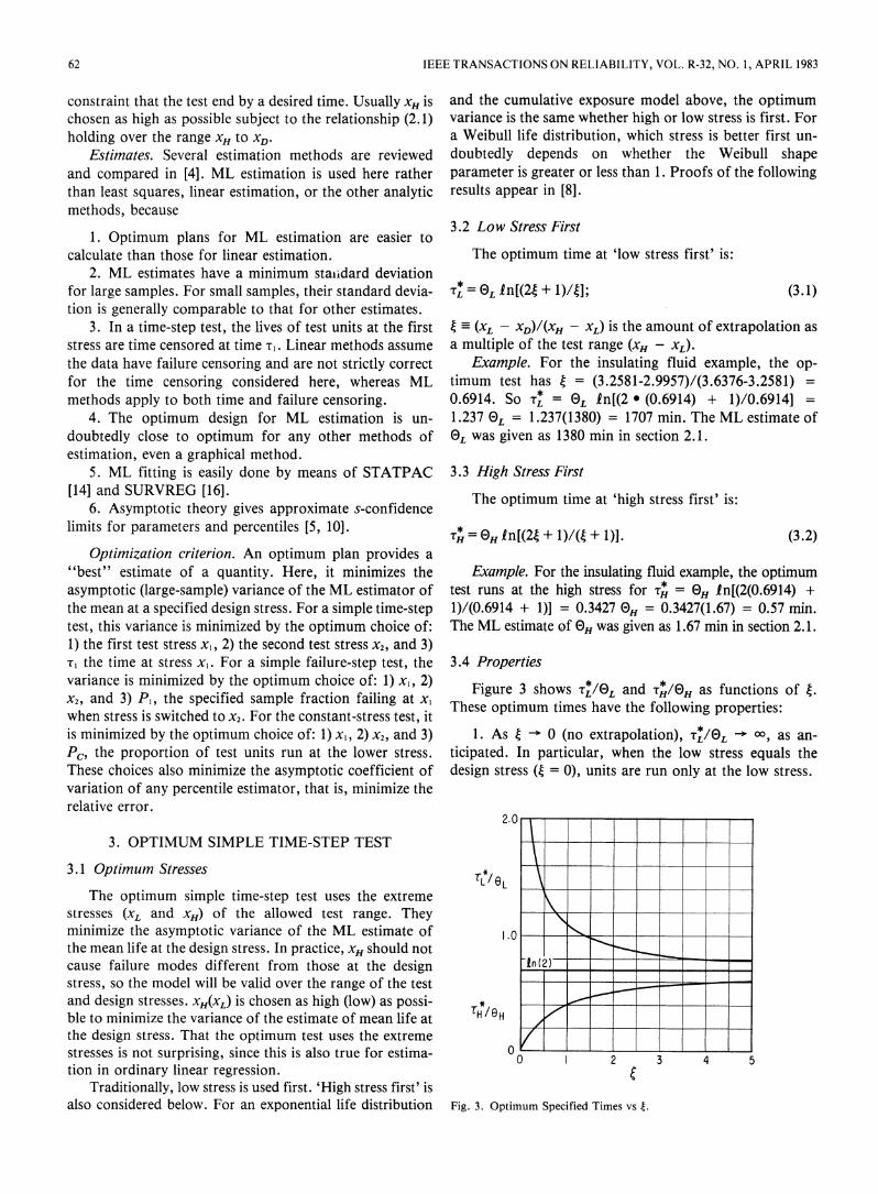
3.2 Low Stress First1. Optimum plans for ML estimation are easier to

calculate than those for linear estimation. The optimum time at 'low stress first' is:2. ML estimates have a minimum statidard deviation

for large samples. For small samples, their standard devia- TL = 0L 2n[(24 + 1)/4]; (3.1)tion is generally comparable to that for other estimates.

3. In a time-step test, the lives of test units at the first 4 - (XL - XD)/(XH - XL) is the amount of extrapolation asstress are time censored at time T1. Linear methods assume a multiple of the test range (XH - XL).the data have failure censoring and are not strictly correct Example. For the insulating fluid example, the op-for the time censoring considered here, whereas ML timum test has 4 = (3.2581-2.9957)/(3.6376-3.2581) =methods apply to both time and failure censoring. 0.6914. So TL = OL In[(2 * (0.6914) + 1)/0.6914] =

4. The optimum design for ML estimation is un- 1.237 eL = 1.237(1380) = 1707 min. The ML estimate ofdoubtedly close to optimum for any other methods of )L was given as 1380 min in section 2.1.estimation, even a graphical method.

5. ML fitting is easily done by means of STATPAC 3.3 High Stress First[14] and SURVREG [16].. . .,.[14] andSURVREG [16]. ~~~~The optimum time at 'high stress first' iS:6. Asymptotic theory gives approximate s-confidencelimits for parameters and percentiles [5, 10]. TH= 0H ln[(24+ 1)/( + 1)]. (3.2)

Optimization criterion. An optimum plan provides a"best" estimate of a quantity. Here, it minimizes the Example. For the insulating fluid example, the optimumasymptotic (large-sample) variance of the ML estimator of test runs at the high stress for *r = eH In[(2(0.6914) +the mean at a specified design stress. For a simple time-step 1)/(0.6914 + 1)] = 0.3427 OH = 0.3427(1.67) = 0.57 min.test, this variance is minimized by the optimum choice of: The ML estimate of 0H was given as 1.67 min in section 2.1.1) the first test stress x, 2) the second test stress x2, and 3)T1 the time at stress x,. For a simple failure-step test, the 3.4 Propertiesvariance is minimized by the optimum choice of: 1) xl, 2) Figure 3 shows .r*/eL and */G as functions of4x2, and 3) Pi, the specified sample fraction failing at x Twhen stress is switched to x2. For the constant-stress test, itis minimized by the optimum choice of: 1) x,, 2) x2, and 3) 1. As 4 0 (no extrapolation), T-r/eL --> o, as an-Pc' the proportion of test units run at the lower stress. ticipated. In particular, when the low stress equals theThese choices also minimize the asymptotic coefficient of design stress (4 = 0), units are run only at the low stress.variation of any percentile estimator, that is, minimize therelative error.

3. OPTIMUM SIMPLE TIME-STEP TEST

3.1 Optimum Stresses TL*/L |

The optimum simple time-step test uses the extremestresses (XL and XH) of the allowed test range. They A -minimize the asymptotic variance of the ML estimate of .0the mean life at the design stress. In practice, XH should notcause failure modes different from those at the design In(2)stress, so the model will be valid over the range of the test| | lland design stresses. XH(XL) iS chosen as high (low) as pOSSi- - __ _ble to minimize the variance of the estimate ofmean life at TH /@Hthe design stress. That the optimum test uses the extreme Vlllllllll

tion in ordinary linear regression.Traditionally, low stress is used first. 'High stress first' is

also considered below. For an exponential life distribution Fig. 3. Optimum Specified Times vs 4.


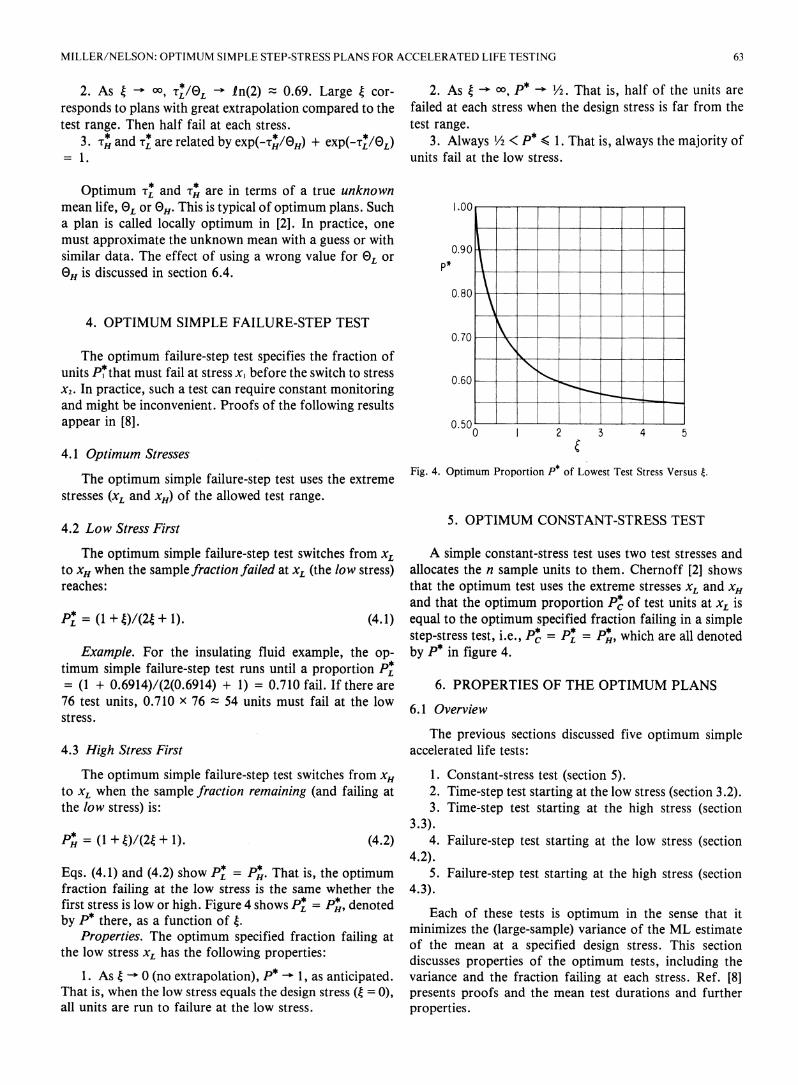
2. As 4 -- 0, T -* In(2) - 0.69. Large 4 cor- 2. As 4 oo, P* l/2. That is, half of the units areresponds to plans with great extrapolation compared to the failed at each stress when the design stress is far from thetest range. Then half fail at each stress. test range.

3. TH and TL are related by exp(- */e)H) + exp(--r//eL) 3. Always 1/2< P* < 1. That is, always the majority of= 1. units fail at the low stress.

Optimum TL and TH are in terms of a true unknownmean life, EL or 0H. This is typical of optimum plans. Such l .00C.a plan is called locally optimum in [2]. In practice, onemust approximate the unknown mean with a guess or with

0

similar data. The effect of using a wrong value for 0L or °l0H is discussed in section 6.4.

0.80 ---

4. OPTIMUM SIMPLE FAILURE-STEP TEST0.70 -_ __

The optimum failure-step test specifies the fraction of _ _units P* that must fail at stress x1 before the switch to stress 060x2. In practice, such a test can require constant monitoring 0.60and might be inconvenient. Proofs of the following resultsappear in [8]. 0.500 2 3

4.1 Optimum Stresses

The optimum simple failure-step test uses the extreme Fig. 4. Optimum Proportion P* of Lowest Test Stress Versus 4.stresses (XL and xH) of the allowed test range.

4.2 Low Stress First 5. OPTIMUM CONSTANT-STRESS TEST

The optimum simple failure-step test switches from XL A simple constant-stress test uses two test stresses andto XH when the sample fraction failed at XL (the low stress) allocates the n sample units to them. Chernoff [2] showsreaches: that the optimum test uses the extreme stresses XL and XH

and that the optimum proportion PC of test units at XL isPL = (1 + 4)/(24 + 1). (4.1) equal to the optimum specified fraction failing in a simple

step-stress test, i.e., PC = PL = P*, which are all denotedExample. For the insulating fluid example, the op- by P* in figure 4.

timum simple failure-step test runs until a proportion PL= (1 + 0.6914)/(2(0.6914) + 1) = 0.710 fail. If there are 6. PROPERTIES OF THE OPTIMUM PLANS76 test units, 0.710 x 76 - 54 units must fail at the low

stress. ~~~~~~~~~~~6.1 Overviewstress.The previous sections discussed five optimum simple

4.3 High Stress First accelerated life tests:

The optimum simple failure-step test switches from XH 1. Constant-stress test (section 5).to XL when the sample fraction remaining (and failing at 2. Time-step test starting at the low stress (section 3.2).the low stress) is: 3. Time-step test starting at the high stress (section

3.3).PH = (1 + 4)/(24 + 1). (4.2) 4. Failure-step test starting at the low stress (section

4.2).Eqs. (4.1) and (4.2) show PL = PH. That is, the optimum 5. Failure-step test starting at the high stress (sectionfraction failing at the low stress is the same whether the 4.3).first stress is low or high. Figure 4 shows PL = PH, denoted Eahotestssispimmntesnetatt

by~P. there, aafucino4. minimizes the (large-sample) variance of the ML estimateProertes.Theoptmumspcifed racionfaiingatof the mean at a specified design stress. This section

the lw stessL hasthe olloing poperies:discusses properties of the optimum tests, including the1. As 4 - 0 (no extrapolation), P* -~1, as anticipated. variance and the fraction failing at each stress. Ref. [8]

That is, when the low stress equals the design stress (4 = 0), presents proofs and the mean test durations and furtherall units are run to failure at the low stress. properties.


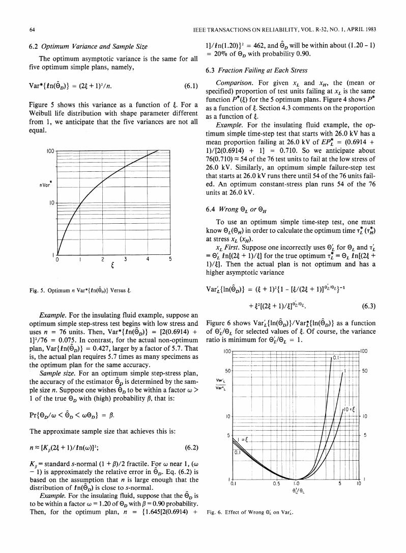
6.2 Optimum Variance and Sample Size 11/in(1.20)}2 = 462, and OD will be within about (1.20 - 1)= 20%of eD with probability 0.90.

The optimum asymptotic variance is the same for allfive optimum simple plans, namely,. .fiv optimum simple plans, namely, 6.3 Fraction Failing at Each Stress

Var*{in(AD)} = (24 + 1)2/n (6.1) Comparison. For given xL and XH, the (mean orspecified) proportion of test units failing at XL 1S the samefunction P*(4) for the 5 optimum plans. Figure 4 shows P*

Figure 5 shows this variance as a function of 4. For a as a function of 4 Section 4.3 comments on the proportionWeibull life distribution with shape parameter different as a function of .from 1, we anticipate that the five variances are not all Example. For the insulating fluid example, the op-equal. timum simple time-step test that starts with 26.0 kV has a

mean proportion failing at 26.0 kV of EPL = (0.6914 +l00 - _ 1)/[2(0.6914) + 1] - 0.710. So we anticipate about

76(0.710) = 54 of the 76 test units to fail at the low stress oft____ 7f___ 26.0 kV. Similarly, an optimum simple failure-step test

____ ___ __I_l that starts at 26.0 kV runs there until 54 of the 76 units fail-n Var Z/ ed. An optimum constant-stress plan runs 54 of the 76

units at 26.0 kV.10-

6.4 Wrong eLoreH

To use an optimum simple time-step test, one mustknow Oe(GH) in order to calculate the optimum time Tr (Tr)at stress XL (XH).

_____|___d_ I__________ xLFirst. Suppose one incorrectly uses Oj for Oe and -r0 ( 2 35 4 ' i = 0L In[(24 + 1)/1] for the true optimum TL = 0L In[(24 +

l)/4]. Then the actual plan is not optimum and has ahigher asymptotic variance

Fig. 5. Optimum n Var*{in(e6D)} Versus 4. Var[{ln(kD)} = (4 + 1)1{1 - [4/(24 + 1)]IL/eL}-1

+ 42[(24 + I)/4]EL/eL. (6.3)Example. For the insulating fluid example, suppose an

optimum simple step-stress test begins with low stress and Figure 6 shows Var'{ln(eD)}/Var{ln(OD)} as a functionuses n = 76 units. Then, Var*{in(0D)} = [2(0.6914) + of OJGL for selected values of 4. Of course, the variance112/76 = 0.075. In contrast, for the actual non-optimum ratio is minimum for 3L/'L = 1.plan, Var{in(OD)} = 0.427, larger by a factor of 5.7. That 100is, the actual plan requires 5.7 times as many specimens as -- othe optimum plan for the same accuracy. - -

Sample size. For an optimum simple step-stress plan, 50 - 50the accuracy of the estimator G, is determined by the sam- Van. I_iple size n. Suppose one wishes OD to be within a factor )>Var>L1 of the trueeD with (high) probability ,that is:

t0Pr{OD/cJ) < OD < (AJOD} = lo f 10

The approximate sample size that achieves this is: 5 I 5

n WoMKg3(2S, + W)/lN(0)]2; (6.2) X _ /

K,, =standard s-normal (1 + I/2fractile. For co near 1, (co C I Iv- 1) is approximately the relative error in G3D. Eq. (6.2) isI X |ll|based on the assumption that n is large enough that the .distribution of in(GD) is close to s-normal. 01 5 0 0

Example. For the insulating fluid, suppose that the 0D iSeLLto be within a factor co = 1.20 of GD with 0=0.90 probability.Then, for the optimum plan, n = { 1.645(2(0.6914) + Fig. 6. Effect of Wrong OL on VarL.


Figure 6 shows that underestimating E)L by some factor [8] R. Miller, W.B. Nelson, "Optimum simple step-stress tests for ac-increases Var2 less than does overestimating E)L by the celerated life testing," General Electric Research & DevelopmentL

TIS Report 79CRD262, 1979.*saefactor. So it iS safer to underestimate eL. TI eot7CD6,17.samefcor o i . , L [91 W.B. Nelson, "Statistical methods for accelerated life testXH First. Suppose one incorrectly uses O' for O. TheH H data-The inverse power law model," General Electric Research &

asymptotic variance is: Development TIS Report 71-C-011, 1970.* Graphical methodspublished in IEEE Trans. Reliability, vol R-21, 1972 Feb, pp 2-11;

Var'{ln(QD)} = 42{1 [( + 1)/(24 + 1)] OH/OH} -1 correction, p 195.* Least squares methods published in IEEE Trans.Reliability, vol R-24, Jun 1975, pp 103-106.

)2[(24+ ixiO'..8/O@, [10] W.B. Nelson, "Faster accelerated life testing by step-stress-models+ (1+ 4)[24 1)14+)](64) and data analyses," General Electric Research & Development TIS

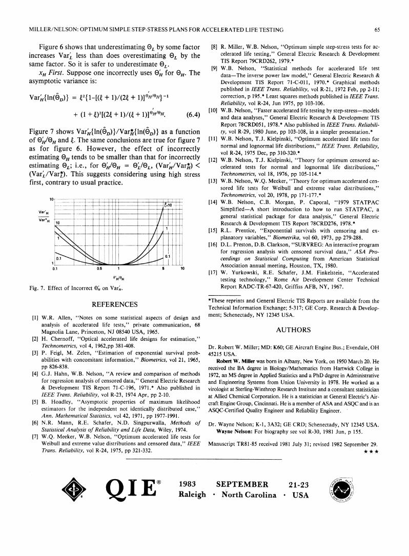
Report 78CRD051, 1978.* Also published in IEEE Trans. Reliabili-Figure 7 shows Var'{ln(eD)}/VarH{ln(0D)} as a function ty, vol R-29, 1980 June, pp 103-108, in a simpler presentation.*of 3/(0H and 4. The same conclusions are true for figure 7 [11] W.B. Nelson, T.J. Kielpinski, "Optimum accelerated life tests for

for figure 6. However, the effect of incorrectly normal and lognormal life distributions," IEEE Trans. Reliability,as for figure 6. However, the effect of Incorrectly vol R-24, 1975 Dec, pp 310-320.*estimating E0H tends to be smaller than that for incorrectly [12] W.B. Nelson, T.J. Kielpinski, "Theory for optimum censored ac-estimating 0L; i.e., for E3/E)H = O'L/OL, (Var'/VarH) < celerated tests for normal and lognormal life distributions,"(Var2/Var*). This suggests considering using high stress Technometrics, vol 18, 1976, pp 105-114.*first, contrary to usual practice. [13] W.B. Nelson, W.Q. Meeker, "Theory for optimum accelerated cen-

sored life tests for Weibull and extreme value distributions,"Technometrics, vol 20, 1978, pp 171-177.*

10 Tici- ---=--F =---t_ X- -_Z ~ -7 [14] W.B. Nelson, C.B. Morgan, P. Caporal, "1979 STATPAC

L--'____ ___ _ _ + __ ! j }i HISimplified-A short introduction to how to run STATPAC, aVar H -_ ls

Va* __ ____ __ general statistical package for data analysis," General Electricr H 10 __ __ _ __ -4 _ Research & Development TIS Report 78CRD276, 1978.*I_ _ _ 4 1L)1_ [15] R.L. Prentice, "Exponential survivals with censoring and ex-

1\\ / / planatory variables," Biometrika, vol 60, 1973, pp 279-288.- 2- L ___ __ - 9 _[16] D.L. Preston, D.B. Clarkson, "SURVREG: An interactive program

for regression analysis with censored survival data," ASA Pro-0.1 1 z G D0.1 ceedings on Statistical Computing from American Statistical0__1 0 5

- Association annual meeting, Houston, TX, 1980.[17] W. Yurkowski, R.E. Schafer, J.M. Finkelstein, "Accelerated

OH/0H testing technology," Rome Air Development Center TechnicalFig. 7. Effect of Incorrect EH on VarA. Report RADC-TR-67-420, Griffiss AFB, NY, 1967.

REFERENCES *These reprints and General Electric TIS Reports are available from theTechnical Information Exchange; 5-317; GE Corp. Research & Develop-ment; SchncayNY135UA[1] W.R. Allen, "Notes oIn some statistical aspects of design and henectady, NY 12345 USA.

analysis of accelerated life tests," private communication, 68Magnolia Lane, Princeton, NJ 08540 USA, 1965. AUTHORS

[2] H. Chernoff, "Optical accelerated life designs for estimation,"Technometrics, vol 4, 1962,pp 381-408. Dr. Robert W. Miller; MD: K60; GE Aircraft Engine Bus.; Evendale, OH

[3] P. Feigl, M. Zelen, "Estimation of exponential survival prob- 45215 USA.abilities with concomitant information," Biometrics, vol 21, 1965, Robert W. Miller was born in Albany, New York, on 1950 March 20. Hepp 826-838. received the BA degree in Biology/Mathematics from Hartwick College in

[4] G.J. Hahn, W.B. Nelson, "A review and comparison of methods 1972, an MS degree in Applied Statistics and a PhD degree in Administrativefor regression analysis of censored data," General Electric Research and Engineering Systems from Union University in 1978. He worked as a& Development TIS Report 71-C-196, 1971.* Also published in virologist at Sterling-Winthrop Research Institute and a consultant statisticianIEEE Trans. Reliability, vol R-23, 1974 Apr, pp 2-10. at Allied Chemical Corporation. He is a statistician at General Electric's Air-

[5] B. Hoadley, "Asymptotic properties of maximum likelihood craft Engine Group, Cincinnati. He is a member ofASA and ASQC and is anestimators for the independent not identically distributed case," ASQC-Certified Quality Engineer and Reliability Engineer.Ann. Mathematical Statistics, vol 42, 1971, pp 1977-1991.

[61 N.R. Mann, R.E. Schafer, N.D. Singpurwalla, Methods of Dr. Wayne Nelson; K-1, 3A32; GE CRD; Schenectady, NY 12345 USA.Statistical Analysis of Reliability and Life Data, Wiley, 1974. Wayne Nelson: For biography see vol R-30, 1981 Jun, p 155.

[7] W.Q. Meeker, W.B. Nelson, "Optimum accelerated life tests forWeibull and extreme value distributions and censored data," IEEE Manuscript TR81-85 received 1981 July 31; revised 1982 September 29.Trans. Reliability, vol R-24, 1975, pp 321-332.

sTII1 1983 SEPTEMBER 21-23 *j6

* st Raleigh *North Carolina *USA g

Optimum Simple Step-stress Plans for Accelerated Life Testing

Documents

Transcript of Optimum Simple Step-stress Plans for Accelerated Life Testing