Optimum Parameters for Optimum Parameters for CrostonCroston

Intermittent Demand MethodsIntermittent Demand Methods

The 32The 32ndnd Annual International Symposium on ForecastingAnnual International Symposium on Forecasting

www.lancs.ac.uk

NikolaosNikolaos KourentzesKourentzesLancaster University Management School

The 32The 32ndnd Annual International Symposium on ForecastingAnnual International Symposium on Forecasting

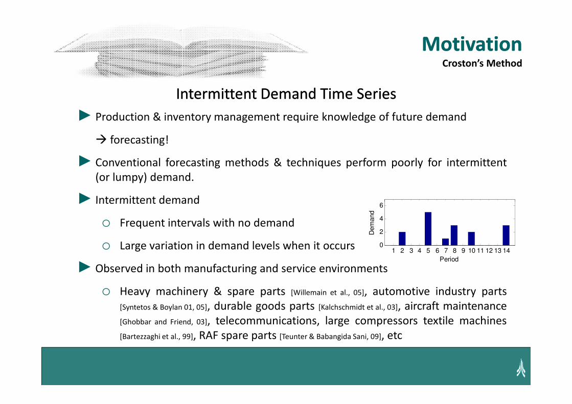
► Production & inventory management require knowledge of future demand

� forecasting!

► Conventional forecasting methods & techniques perform poorly for intermittent

(or lumpy) demand.

► Intermittent demand

Intermittent Demand Time SeriesIntermittent Demand Time Series

6

MotivationMotivationCroston’s Method

► Intermittent demand

o Frequent intervals with no demand

o Large variation in demand levels when it occurs

► Observed in both manufacturing and service environments

o Heavy machinery & spare parts [Willemain et al., 05], automotive industry parts

[Syntetos & Boylan 01, 05], durable goods parts [Kalchschmidt et al., 03], aircraft maintenance

[Ghobbar and Friend, 03], telecommunications, large compressors textile machines

[Bartezzaghi et al., 99], RAF spare parts [Teunter & Babangida Sani, 09], etc

1 2 3 4 5 6 7 8 9 10 11 12 13 140

2

4

6

Period

Dem

and

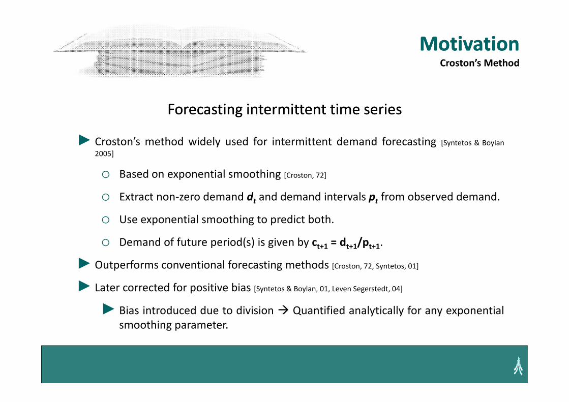
► Croston’s method widely used for intermittent demand forecasting [Syntetos & Boylan

2005]

o Based on exponential smoothing [Croston, 72]

o Extract non-zero demand dt and demand intervals pt from observed demand.

Forecasting intermittent time seriesForecasting intermittent time series

MotivationMotivationCroston’s Method

o Extract non-zero demand dt and demand intervals pt from observed demand.

o Use exponential smoothing to predict both.

o Demand of future period(s) is given by ct+1 = dt+1/pt+1.

► Outperforms conventional forecasting methods [Croston, 72, Syntetos, 01]

► Later corrected for positive bias [Syntetos & Boylan, 01, Leven Segerstedt, 04]

► Bias introduced due to division � Quantified analytically for any exponential

smoothing parameter.

MotivationMotivationCroston’s Method

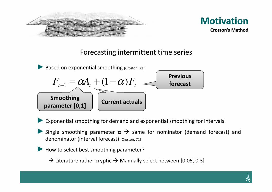
► Based on exponential smoothing [Croston, 72]

Forecasting intermittent time seriesForecasting intermittent time series

tttFAF )1(

1αα −+=

+

Previous

forecast

Smoothing

► Exponential smoothing for demand and exponential smoothing for intervals

► Single smoothing parameter α � same for nominator (demand forecast) and

denominator (interval forecast) [Croston, 72]

► How to select best smoothing parameter?

� Literature rather cryptic � Manually select between [0.05, 0.3]

Current actualsSmoothing

parameter [0,1]

Intermittent DemandIntermittent DemandCroston’s Method

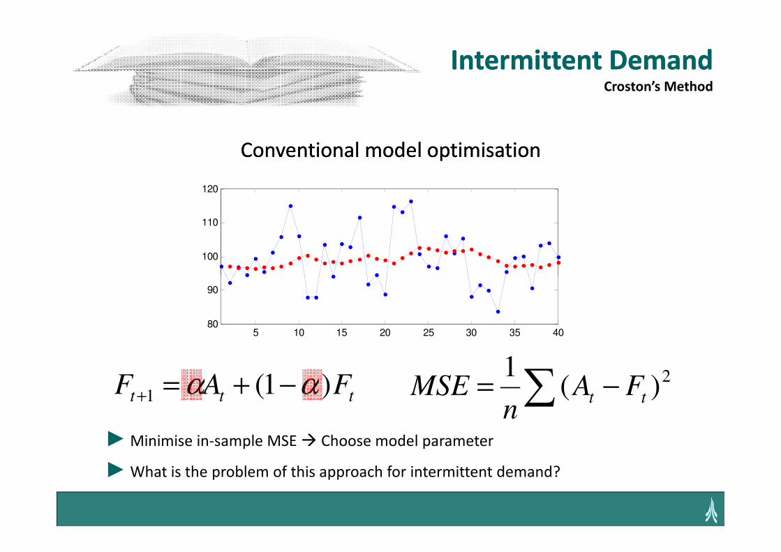
Conventional model optimisationConventional model optimisation

100

110

120

►Minimise in-sample MSE � Choose model parameter

►What is the problem of this approach for intermittent demand?

tttFAF )1(

1αα −+=

+ ∑ −=2

)(1

ttFA

nMSE

5 10 15 20 25 30 35 4080

90

Measuring PerformanceMeasuring Performance

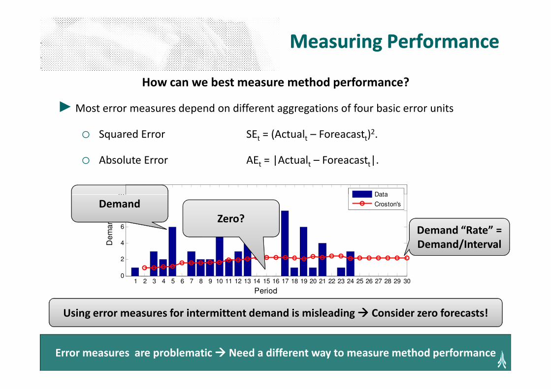
How can we best measure method performance?

►Most error measures depend on different aggregations of four basic error units

o Squared Error SEt = (Actualt – Foreacastt)2.

o Absolute Error AEt = |Actualt – Foreacastt|.

10

Data

1 2 3 4 5 6 7 8 9 10 11 12 13 14 15 16 17 18 19 20 21 22 23 24 25 26 27 28 29 300

2

4

6

8

10

Period

De

ma

nd

Data

Croston's

Error measures are problematic ���� Need a different way to measure method performance

Demand “Rate” =

Demand/Interval

Demand

Zero?

Using error measures for intermittent demand is misleading ���� Consider zero forecasts!

Optimising Optimising Croston’sCroston’s

A novel optimization method on inventory metrics

► Simulate inventory

o Track total stock

o Track total backlog

oo Track realised service levels

► Consider lead times, inventory policy and target service levels

► For each item (time series) run a simulation based on the in-sample data

Optimising Optimising Croston’sCroston’s

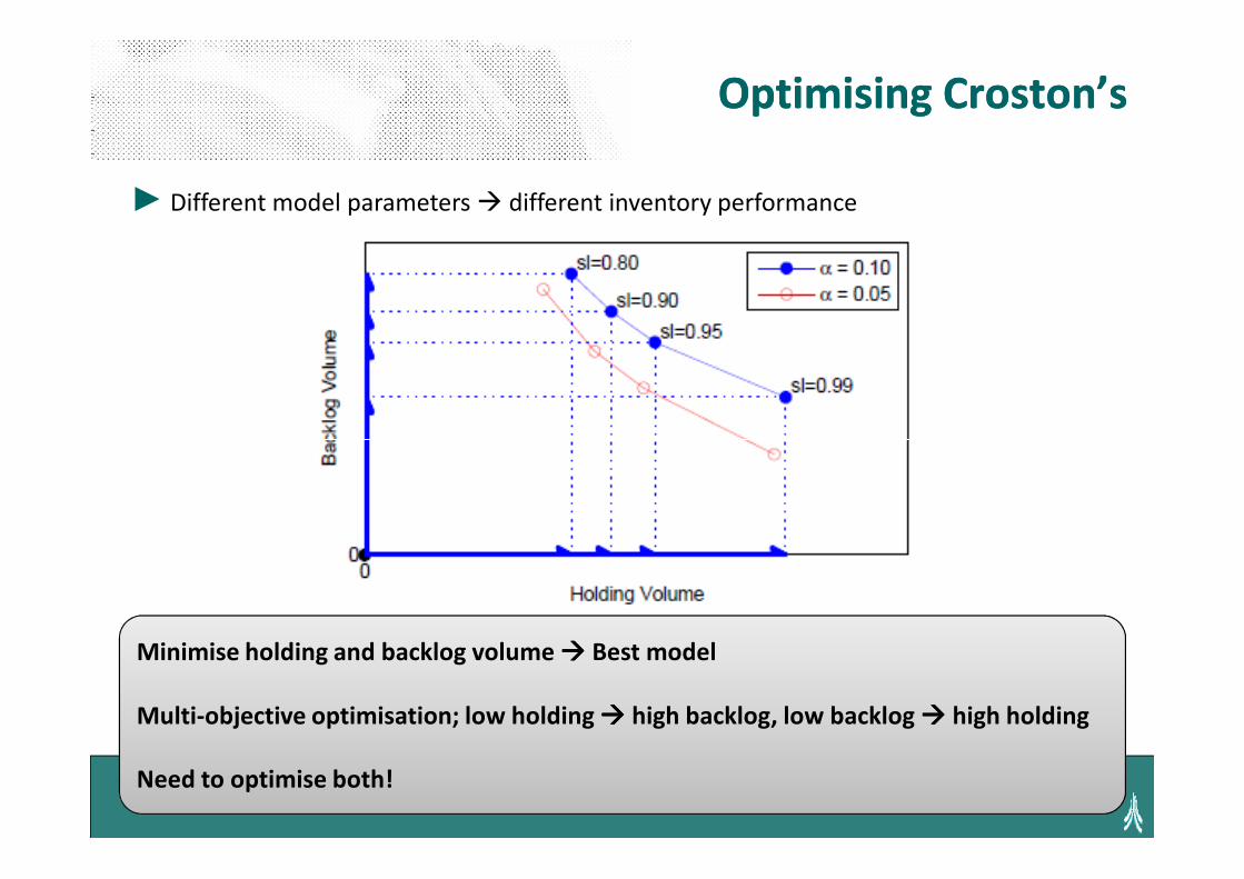
► Different model parameters � different inventory performance

Minimise holding and backlog volume ���� Best model

Multi-objective optimisation; low holding ���� high backlog, low backlog ���� high holding

Need to optimise both!

Optimising Optimising Croston’sCroston’s

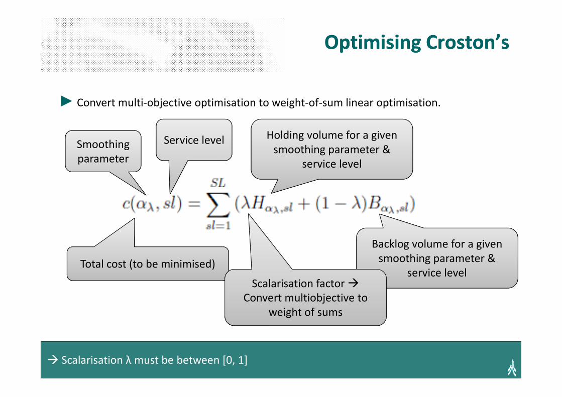
► Convert multi-objective optimisation to weight-of-sum linear optimisation.

Holding volume for a given

smoothing parameter &

service level

Smoothing

parameter

Service level

Total cost (to be minimised)

Backlog volume for a given

smoothing parameter &

service levelScalarisation factor �

Convert multiobjective to

weight of sums

� Scalarisation λ must be between [0, 1]

Optimising Optimising Croston’sCroston’s

Identification of λ and α parameters

► For each λ find optimum smoothing parameter α.

► Find combination of λ and α that gives minimum total cost.

► Select that α as the result of the optimisation

► λ is not related to underage or overage cost � That is the service level!

► Several combinations of λ & α may have same cost � Indifferent � Paretto optimal

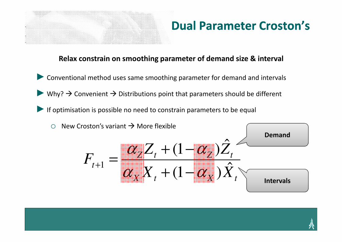
Dual Parameter Dual Parameter Croston’sCroston’s

Relax constrain on smoothing parameter of demand size & interval

► Conventional method uses same smoothing parameter for demand and intervals

►Why? � Convenient � Distributions point that parameters should be different

► If optimisation is possible no need to constrain parameters to be equal

oo New Croston’s variant � More flexible

tXtX

tZtZ

t

XX

ZZF

ˆ)1(

ˆ)1(1

αα

αα

−+

−+=

+

Demand

Intervals

Empirical EvaluationEmpirical Evaluation

Experimental Setup

► Simulate inventory for lead times L = 1, 3, 6

► Simulate service levels 80%, 90%, 95%, 99%

► Data: Empirical distributions from Syntetos and Boylan (2005) � Automotive spare

parts.

► To test data conditions multiply empirical distributions by 1, 3, 5 � More

intermittency

► Each of 9 simulations (3 lead times X 3 multipliers) has 1000 time series

► Each time series: 36 observations in-sample

100 observations burn-in and 100 observations out-of-sample

► Track service levels, holding volume and backlog volume

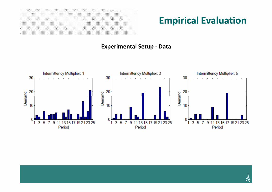
Empirical EvaluationEmpirical Evaluation

Experimental Setup - Data

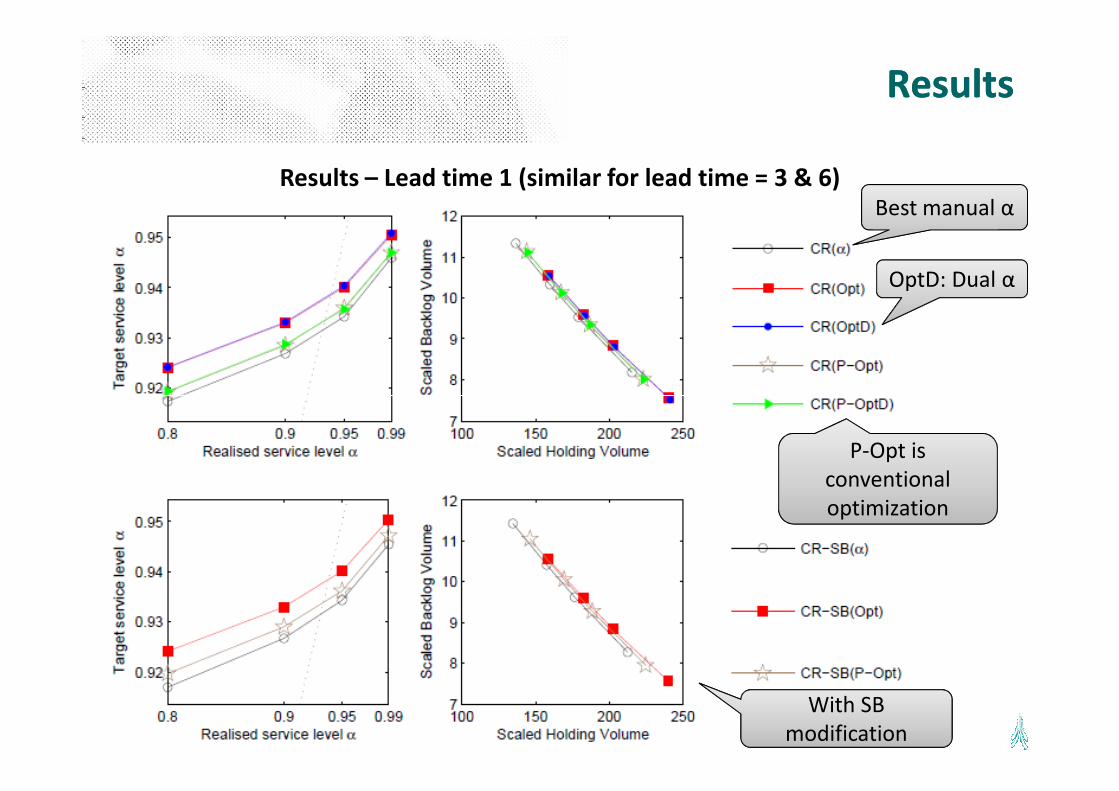
ResultsResults

Results – Lead time 1 (similar for lead time = 3 & 6)Best manual α

OptD: Dual α

P-Opt is

conventional

optimization

With SB With SB

modification

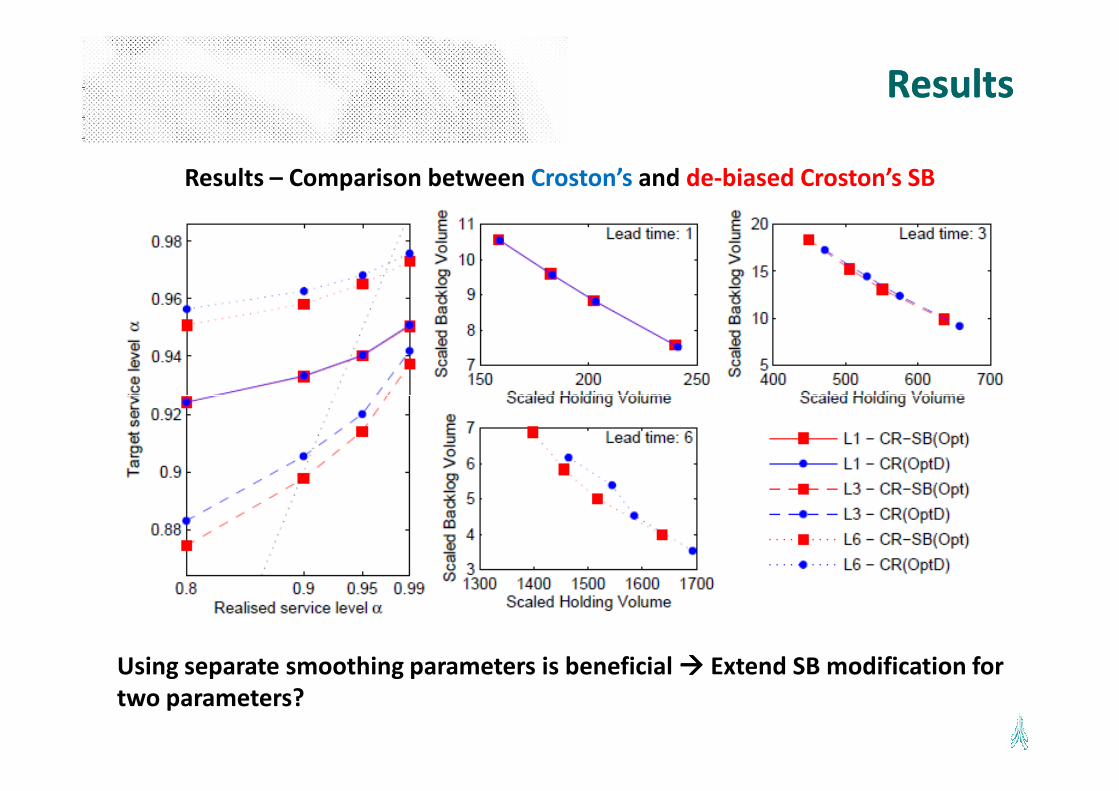
ResultsResults

Results – Comparison between Croston’s and de-biased Croston’s SB

Using separate smoothing parameters is beneficial ���� Extend SB modification for

two parameters?

ConclusionsConclusions

►Optimisation on inventory metrics performs well � Bootstrapping in-sample

provided no gains

►Better than manually presetting parameters or conventional optimisation on

accuracy metrics

►►Results hold for different lead times and different intermittency levels

►Using different smoothing parameter for the non-zero demand and the inter-

demand intervals better than standard approach in the literature (using

single parameter for both)

Nikolaos KourentzesLancaster University Management School

Centre for Forecasting

Lancaster, LA1 4YX, UK

Tel. +44 (0) 7960271368

email n.kourentzes@lancaster.ac.uk

Optimising Optimising Croston’sCroston’s

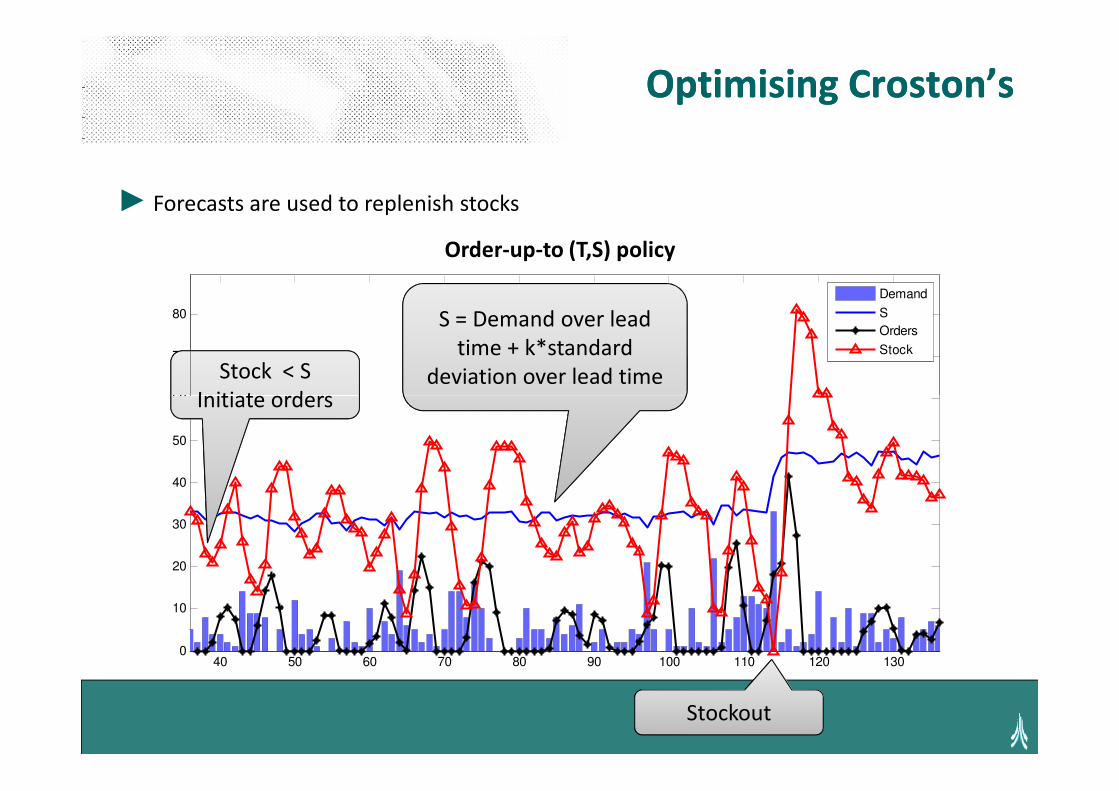
► Forecasts are used to replenish stocks

Order-up-to (T,S) policy

60

70

80

Demand

S

Orders

Stock

Stock < S

Initiate orders

S = Demand over lead

time + k*standard

deviation over lead time

40 50 60 70 80 90 100 110 120 1300

10

20

30

40

50

60

Stockout

Initiate orders