OPTIMUM EXPERIMENTAL DESIGN BY SHAPE OPTIMIZATION … · Shape Optimization of Specimens in Linear...

OPTIMUM EXPERIMENTAL DESIGN BYSHAPE OPTIMIZATION OF SPECIMENS IN

LINEAR ELASTICITY

Tommy Etling* Roland Herzog†

February 10, 2018

The identification of Lamé parameters in linear elasticity is considered.An optimum experimental design problem is formulated, which aims atminimizing the size of an associated confidence ellipsoid by optimizing theshape of the specimen. Representations of the Eulerian shape derivativeand the shape gradient are derived by means of shape calculus and adjointtechniques. Numerical experiments are conducted, yielding specimens ofimproved shape.

KEYWORDS: optimum experimental design; shape optimization; Eulerian derivative;shape gradient; linear elasticity; Lamé parameters; confidence ellipsoid

1 INTRODUCTION

Optimum experimental design (OED) is a well established technique which aims atimproving experimental setups in order to increase the precision of parameter estima-tion in the face of measurement errors. To date, OED is still mostly used for modelswhich are described by ordinary differential equations or differential-algebraic equa-tions, e.g., in chemical engineering and biology; see for instance Skanda, Lebiedz, 2010;Bock, Körkel, Schlöder, 2013, Fedorov, Leonov, 2014, Chapter 7 for recent contributions.

*Technische Universität Chemnitz, Faculty of Mathematics, Professorship Numerical Mathematics (Par-tial Differential Equations), D–09107 Chemnitz, Germany, [email protected],https://www.tu-chemnitz.de/∼ett

†Technische Universität Chemnitz, Faculty of Mathematics, Professorship Numerical Mathematics (Par-tial Differential Equations), D–09107 Chemnitz, Germany, [email protected],https://www.tu-chemnitz.de/herzog

mailto:[email protected]

https://www.tu-chemnitz.de/~ett

mailto:[email protected]

https://www.tu-chemnitz.de/herzog

Shape Optimization of Specimens in Linear Elasticity Etling, Herzog

In this context, typical experimental conditions, which serve as optimization variables,include initial conditions, right hand side sources, and observation times. Extensions ofOED to models involving partial differential equations were considered, for instance,in Ito, Kunisch, 1995; Ucinski, 2005; Carraro, 2005; Lahmer, Kaltenbacher, Schulz, 2008;Haber, Horesh, Tenorio, 2008; Bambach, Heinkenschloss, Herty, 2013; Herzog, Riedel,2015; Herzog, Ospald, 2017.

In this paper, we consider an OED problem in linear elasticity, where the model is de-scribed by an elliptic partial differential equation. In a typical experimental setup thetwo Lamé parameters, which determine the constitutive behavior of the material in theisotropic case, are to be identified from the response of a specimen subjected to tensilestress. Our objective is to increase the precision in the estimation of these parameters,expressed here in terms of the A-criterion applied to the Fisher information matrix.

The main novelty of our approach is that we treat the shape of the specimen as an exper-imental condition. Following the Lagrangian strategy for shape optimization problemsof Céa, 1986; Delfour, Zolésio, 1988, recently revisited by Sturm, 2015; Laurain, Sturm,2016, we derive a volume representation of the Eulerian shape derivative of the OEDobjective. Similar to other classical approaches as in Sokołowski, Zolésio, 1992, theLagrangian approach leads to an adjoint-based representation of the shape derivative,but it avoids material or local shape derivatives of the state. As in Schulz, Siebenborn,Welker, 2016, we then employ the volume representation of the shape derivative toobtain a shape gradient w.r.t. an H1-based inner product, which drives a gradient de-scent algorithm. Numerical experiments demonstrate the viability of our approach andreveal new and interesting specimen shapes for tensile experiments.

We are aware of only one publication where geometry was used as an experimentalcondition. In Logashenko et al., 2001, the boundary of a measurement device was dis-cretized by a small number of shape parameters and optimized using a derivative-freeoptimization approach to improve the estimation precision of two unknown parame-ters in a Bingham flow model.

The material is organized as follows. In Section 2, we describe the parameter estimationproblem under consideration for a given shape of the specimen. We also quantify theestimation accuracy in terms of the A-criterion applied to the Fisher information ma-trix, which subsequently serves as our optimality criterion. Section 3 is devoted to theshape optimization problem and it contains as our main result the volume representa-tion of the Eulerian shape derivative as well as the H1-based shape gradient. Numericalexperiments in two space dimensions are presented in Section 4. We conclude with anoutlook in Section 5.

2 PARAMETER ESTIMATION IN LINEAR ELASTICITY

In this section we briefly review parameter estimation problems in linear elasticity withinfinitesimal strains. We refer to Bonnet, Constantinescu, 2005 for an overview from the

2


mathematical point of view and to Davis, 2004 from the engineering perspective. Wefocus on the deformation of an elastic specimen by the application of certain boundarystresses or boundary displacements. We measure the mean values of the displacementfield in a number of predefined observation areas distributed across the specimen’ssurface. In practice, this is achieved by optical measurement techniques such as videoextensometers. The constitutive parameters are subsequently identified from the mea-sured material response by way of a least-squares approach.

In this paper we concentrate on prismatic specimens with two-dimensional displace-ment fields, but extensions to fully three-dimensional bodies are clearly possible. Othertypes of measurements such as strain gauges are possible as well but they will not bediscussed here. In the interest of clarity of the presentation, we focus primarily on asingle stress-driven experiment with given boundary traction.

2.1 FORWARD PROBLEM

Let us denote by Ω ⊂ R2 the lateral cross section of the elastic specimen; see Figure 2.1.The state variable of the problem is the displacement field u : Ω → R2. We denote byDu the Jacobian of u and by

ε(u) =12(

Du + (Du)>)= sym(Du)

the (linearized) strain tensor. Here and throughout the rest of the paper, ’sym’ denotesthe symmetric part of a matrix.

The forward problem of linear elasticity is described by the equilibrium of forces (grav-ity is neglected),

− div σ = 0 in Ω, (2.1)

together with mixed boundary conditions

σn = g on ΓN , (2.2a)σn = 0 on Γfree, (2.2b)

u = 0 on ΓD. (2.2c)

Herein, σ : Ω→ R2×2sym denotes the stress field with values in the symmetric matrices of

dimension 2× 2. The differential operator div denotes the (row-wise) divergence.

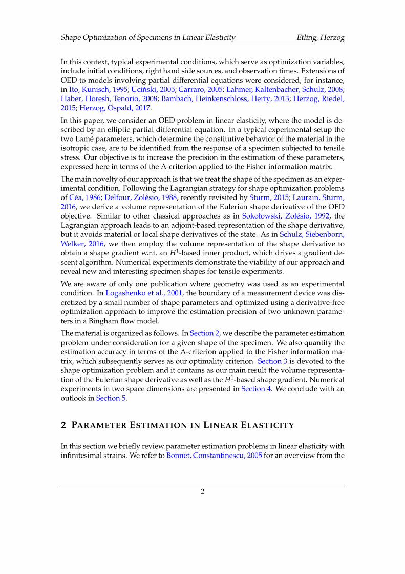
The boundary Γ is divided into three disjoint parts, the traction boundary ΓN , the force-free boundary Γfree, and the clamping boundary ΓD. Moreover, n is the outer unit nor-mal along the boundary Γ. The data g accounts for the applied tensile stress during theexperiment; see again Figure 2.1.

In linear elasticity the relation between stresses σ and strains ε(u) is described by alinear mapping from R2×2

sym into itself. The latter is represented by the fourth-order elas-ticity tensor C, i.e.,

σ = C ε(u) (2.3)

3


gΓD ΓN

Γfree

Γfree

Ω

Figure 2.1: Typical configuration of a specimen in a tensile experiment.

holds pointwise in Ω. The specific form of C in the isotropic case is addressed in Sec-tion 2.2.

We will work with the well-known weak formulation of the state equation (2.1)–(2.3),

Find u ∈ V such that∫

Ωε(v) : C ε(u)dx =

∫ΓN

g · v ds for all v ∈ V . (2.4)

In (2.4), the standard inner product (associated with the Frobenius norm | · |F) betweenmatrices of equal size is defined by A : B := trace(A>B). The state and test space in(2.4) is given by

V := H1D(Ω)2 := u ∈ H1(Ω)2 : u = 0 on ΓD.

Provided that C is coercive, i.e.,

ε : C ε ≥ c |ε|2F for all ε ∈ R2×2sym

with some constant c > 0, it follows from the Lax-Milgram theorem and Korn’s in-equality that (2.4) is uniquely solvable and that the solution depends continuously onthe data g, for instance w.r.t. the topologies of L2(ΓN)

2 and H1(Ω)2.

2.2 IDENTIFICATION PROBLEM

We will be concerned with the case of homogeneous, isotropic elasticity, when C isdescribed by only two parameters. One common parametrization uses the Lamé coef-ficients (λ, µ) with µ > 0 and λ + µ > 0:

C ε = 2 µ ε + λ trace(ε) id2×2 . (2.5)

The second parameter µ is also known as the shear modulus. We mention that we con-sider the so-called plane-stress situation, i.e., the specimen can move freely in thicknessdirection. This will play a role later on.

Clearly, it is impossible to measure the entire displacement state. In practical experi-ments, one encounters for instance measurements of the displacement of selected points

4


of the specimen, as well as measurements of certain strain components. We concentratehere on measurements of the average displacement vector over a number of small ob-servation regions distributed across the specimen’s lateral surface. Since we consider a2D situation, this amounts to interior measurements of the form

Mk u =1|Rk|

∫Rk

u · ek dx, k = 1, . . . , nmeas. (2.6)

Each measurement k belongs to a measurement region Rk ⊂ Ω and a measurementdirection ek, usually ek = (1, 0)> or ek = (0, 1)>. The number of these measurements isdenoted by nmeas. It is not necessary that the measurement regions be disjoint, althoughthis will be the case in our numerical experiments; see Figure 3.1.

The most common approach for the estimation of the elastic parameters (λ, µ) is basedon a least-squares formulation. We assume that each measurement (2.6) is subject toa normally distributed measurement error with zero mean and variance σ2

k . We alsoassume that the measurement errors are independent, i.e., the joint measurement co-variance matrix

Σ = diag(σ2k ), k = 1, . . . , nmeas

is diagonal.

Let us denote by ηk the individual measurements, k = 1, . . . , nmeas. Then the maxi-mum likelihood estimator for the elastic parameters is equivalent to the solution of thefollowing weighted least-squares problem,

Minimize f (p, u) =12

nmeas

∑k=1

σ−2k (Mk u− ηk)

2, (p, u) ∈ P× V

subject to u solving the forward problem (2.4).

(2.7)

Herein, p corresponds to the pair (λ, µ). Moreover, P denotes the open subset of ad-missible parameters, i.e.,

P = (λ, µ) ∈ R2 : µ > 0, λ + µ > 0.

In place of the constrained problem (2.7) it will be convenient to consider the reducedproblem, which depends only on p. To this end we introduce the parameter-to-statemap

R2 ⊃ P 3 p 7→ (p) = u ∈ V , (2.8)

where u solves (2.4). Since S is well defined, the reduced problem becomes

Minimize F (p) := f (p, (p)) =12

nmeas

∑k=1

σ−2k (Mk (p)− ηk)

2, p ∈ P. (2.9)

We emphasize that (2.9) is a nonlinear least-squares problem despite the linear measure-ments and the linearity of the state equation since the unknown parameter vector penters (2.4) through the coefficients and thus S is nonlinear.

5


2.3 SENSITIVITY EQUATION

Let us denote byrk := Mk (p)− ηk, k = 1, . . . , nmeas (2.10)

the (unweighted) residuals of (2.9). For the efficient solution of (2.9), but also for thesubsequent assessment of the accuracy of the estimation we consider the Jacobian J ofthe residual vector w.r.t. p = (p1, p2). Since the measurement operators Mk are linear,we get

Jk,`(p) := Mk∂

∂p`(p), k = 1, . . . , nmeas, ` = 1, 2. (2.11)

By the implicit function theorem and (2.4), we obtain that the sensitivity of the displace-ment field w.r.t. to either of the two parameters, δu` := ∂

∂p`(p), is defined by the unique

solution of the following linearized problem,

Find δu` ∈ V such that∫

Ωε(v) : C ε(δu`)dx = −

∫Ω

ε(v) : C` ε(u)dx for all v ∈ V ,

(2.12)where u = (p). Here we used the abbreviation C` := ∂

∂p`C, and according to (2.5) we

have

Cλ ε :=∂

∂λC ε ≡ trace(ε) id2×2, (2.13a)

Cµ ε :=∂

∂µCµ ≡ 2 ε. (2.13b)

By plugging in the specific form of the measurement operator (2.6), we infer that theentries in the Jacobian (2.11) become

Jk,`(p) =1|Rk|

∫Rk

δu` · ek dx, k = 1, . . . , nmeas, ` = 1, 2. (2.14)

Assumption 2.1. We assume throughout that the Jacobian has rank two, i.e., that bothparameters are, in principle, identifiable from the measurements available.

This assumption does not impose severe restrictions on the measurement setup.

2.4 ACCURACY OF ESTIMATION

Intuitively, parameters in a model can be well identified if their change leads to a sig-nificant model response, or more precisely, a significant response in the observed partof the model. This information is encoded in the Jacobian J (2.11) of the residuals. Wefollow here a classical approach and assess the accuracy of the estimation based on theFisher information matrix (also known as precision matrix)

F(p) = J(p)>Σ−1 J(p) ∈ R2×2. (2.15)

6


We refer the reader to Ucinski, 2005; Pukelsheim, 2006; Pronzato, Pázman, 2013; Fe-dorov, Leonov, 2014 for in-depth material on this topic. Notice that the Fisher infor-mation matrix at p coincides with the inverse of the covariance of the least-squaresestimator when the residuals are linearized about p; see for instance Fedorov, Leonov,2014, Chapter 1.4.2. We therefore denote this covariance matrix by

C(p) = F(p)−1 ∈ R2×2. (2.16)

Notice that the inverse exists due to Assumption 2.1.

Common criteria assessing the precision of the estimation, based on the eigenvaluesλ` of the respective 2× 2 covariance matrix C, are

A-criterion ψA(C) =12

2

∑`=1

λ` =12

trace C, (2.17a)

D-criterion ψD(C) =( 2

∏`=1

λ`

)1/2=(det C

)1/2, (2.17b)

E-criterion ψE(C) = max`=1,2λ`. (2.17c)

These criteria can be related to various geometric quantities associated with approxi-mate confidence ellipsoids in the parameter plane; see for instance Fedorov, Leonov,2014, Section 2.2. While the eigenvectors of C represent the orientation of the semi-axesof the ellipsoid, the square root of the eigenvalues λ`, multiplied with

[Φ−1

χ22(α)]1/2 yield

the length of the corresponding semi-axis. Here α ∈ (0, 1) is a given confidence leveland Φχ2

2denotes the cumulative distribution function (CDF) of the χ2 distribution with

two degrees of freedom. We are going to use, exemplarily, the A-criterion as our op-timization criterion in the sequel, which is proportional to the sum of the eigenvaluesand thus to the average squared length of the semi-axes.

We will also be interested in the precision of the estimation of only one of the two param-eters and we distinguish two cases:

1. When we need to estimate only the `-th parameter, while the other one is given,we replace the full Jacobian J by its `-th column. Consequently, the covariancematrix becomes scalar, the confidence ellipsoid reduces to an interval, and allcriteria in (2.17) become equivalent. They can be best expressed in terms of thediagonal entry F`,` of the full Fisher information matrix (2.15).

2. When both parameters are unknown and need to be estimated from the availablemeasurements, but we are only interested in the precision of the `-th parame-ter, then the quantity of interest becomes C`,`, i.e., the diagonal entry of the fullcovariance matrix (2.16).

In either case, the precision of the estimation of the single relevant parameter can beexpressed in terms of its (marginal) confidence interval. The radius of this interval for

7


the `-th parameter is given by

CI` =[Φ−1

χ21(α)]1/2 [F`,`

]−1/2 in case 1, (2.18a)

CI` =[Φ−1

χ21(α)]1/2 [C`,`

]1/2 in case 2, (2.18b)

where Φχ21

denotes the CDF of the χ2 distribution with one degree of freedom.

3 OPTIMUM EXPERIMENTAL DESIGN BY SHAPE

OPTIMIZATION

In this section we come to the main contributions of this paper. The main and novelidea is to use the geometry of the specimen as an experimental design variable in orderto increase the accuracy in the estimation of the elastic parameters. In other words, onetries to maximize the gain of information obtained through an experiment, measuredin terms of one of the criteria (2.17); we focus here on the A-criterion. This leads to anovel type of an optimum experimental design (OED) problem, which is addressed byshape optimization techniques.

In a typical setup one employs the parameter identification process and the design ofthe subsequent experiment in an alternating fashion known as sequential design; see, forinstance Körkel, Bauer, et al., 1999. During an OED phase, the current parameter set pis either considered fixed at its last known value, or one deems it uncertain and usesa robust optimization framework as for instance in Körkel, Kostina, et al., 2004. Sinceour concern here is to use the shape of the specimen as a novel type of experimentalcondition, we concentrate on the design problem only and consider the value of theelastic parameters p fixed.

Our notation concerning the shape optimization mainly follows Sokołowski, Zolésio,1992. Perturbations Ωt of an initial shape Ω ⊂ R2 will be expressed in terms of asufficiently smooth vector field V : R2 → R2. We use the perturbation of identityapproach, which maps the points x0 ∈ Ω onto Ωt = Tt(Ω) according to

x(t) := Tt(x0) := x0 + t V(x0) (3.1)

for t ≥ 0. Note that T0 = id (the identity) and Ω0 = Ω hold.

The outline of our proposed approach is as follows. First we set up the shape opti-mization problem whose objective expresses the desire to increase the accuracy of theestimation of the elastic parameters. We use the A-criterion (2.17a) based on the covari-ance matrix C from (2.16) for this purpose, but other criteria can be used as well. Sincethe covariance matrix depends on the Jacobian of the residuals, which involves the so-lution of the sensitivity equation, a classical approach based on the chain rule suggeststhat we have to find the (material) derivative of the solution of the sensitivity equation(2.12) w.r.t. the perturbation vector field V . This is however, quite involved due to the

8


state u appearing in the right hand side of (2.12), and not covered by standard shape dif-ferentiation results in elasticity; see Sokołowski, Zolésio, 1992, Chapter 3.5 and Eppler,2010. Therefore, and also in the interest of reduced regularity requirements we resort tothe material derivative-free approach developed by Sturm, 2015; Laurain, Sturm, 2016,which leads directly to an adjoint-based representation of the Eulerian derivative of ourobjective (3.2).

gR1 R2 R3ΓD ΓN

Γfree

Γfree

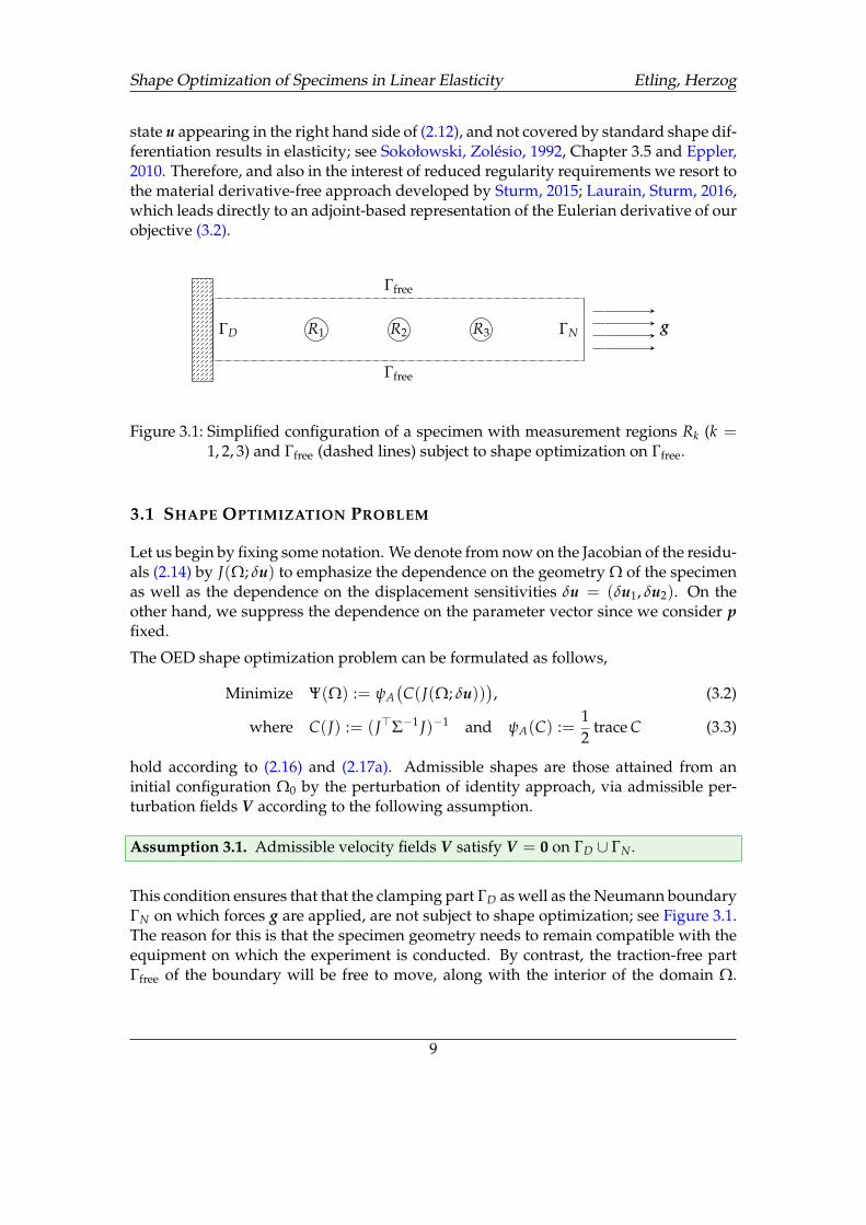
Figure 3.1: Simplified configuration of a specimen with measurement regions Rk (k =1, 2, 3) and Γfree (dashed lines) subject to shape optimization on Γfree.

3.1 SHAPE OPTIMIZATION PROBLEM

Let us begin by fixing some notation. We denote from now on the Jacobian of the residu-als (2.14) by J(Ω; δu) to emphasize the dependence on the geometry Ω of the specimenas well as the dependence on the displacement sensitivities δu = (δu1, δu2). On theother hand, we suppress the dependence on the parameter vector since we consider pfixed.

The OED shape optimization problem can be formulated as follows,

Minimize Ψ(Ω) := ψA(C(J(Ω; δu))

), (3.2)

where C(J) := (J>Σ−1 J)−1 and ψA(C) :=12

trace C (3.3)

hold according to (2.16) and (2.17a). Admissible shapes are those attained from aninitial configuration Ω0 by the perturbation of identity approach, via admissible per-turbation fields V according to the following assumption.

Assumption 3.1. Admissible velocity fields V satisfy V = 0 on ΓD ∪ ΓN .

This condition ensures that that the clamping part ΓD as well as the Neumann boundaryΓN on which forces g are applied, are not subject to shape optimization; see Figure 3.1.The reason for this is that the specimen geometry needs to remain compatible with theequipment on which the experiment is conducted. By contrast, the traction-free partΓfree of the boundary will be free to move, along with the interior of the domain Ω.

9


The situation concerning the measurement regions Rk deserves particular mention. Bydesign, they are going to remain fixed relative to the clamping and forcing boundariesΓD ∪ ΓN . However the material points in the domain Ω ‘underneath’ these regions arefree to move.

In order to characterize the Eulerian derivative dΨ(Ω)[V ] in the direction of a givenperturbation field V we introduce the Lagrangian associated with (3.2) on the perturbeddomain Ωt = Tt(Ω), see (3.1), as follows:

Lt(t, ut, δu1,t, δu2,t, zt, w1,t, w2,t)

=12

trace(

J(Ωt; δut)> Σ−1 J(Ωt; δut)

)−1+∫

Ωt

ε(zt) : C ε(ut)dx

−∫

ΓN,t

g · zt ds +2

∑`=1

∫Ωt

ε(w`,t) : C ε(δu`,t)dx +2

∑`=1

∫Ωt

ε(w`,t) : C` ε(ut)dx. (3.4)

The Jacobian on the perturbed domain is defined as[J(Ωt; δut)

]k,` =

1|Rk|

∫Rk

δu`,t · ek dx, k = 1, . . . , nmeas, ` = 1, 2, (3.5)

compare (2.14). It expresses the fact that the measurement regions will remain indepen-dent of the perturbation field.

The second and third lines in (3.4) denote the weak formulations of the elasticity andsensitivity equations (2.4) and (2.12) on the perturbed domain Ωt, respectively. The ad-joint equations governing the adjoint states zt and w`,t, ` = 1, 2, can be derived, as usual,by differentiating (3.4) w.r.t. the forward and sensitivity state variables ut and δu`,t, re-spectively. As seen below, the adjoint states will only be needed in the unperturbeddomain (t = 0) and therefore will be stated later.

The next step is to pull the Lagrangian back to the unperturbed domain via the sub-stitution rule for integrals. The pulled-back states and adjoint states are defined asut := ut Tt etc. Using the abbreviations

γt = det(DTt), ωt = det(DTt) ‖(DTt)−> n‖,

we obtain the family of pulled-back Lagrangians

Lt(t, ut, δut1, δut

2, zt, wt1, wt

2) =12

trace(

Jt(Ω; δut)> Σ−1 Jt(Ω; δut))−1

+∫

Ωεt(zt) : C εt(ut) γt dx−

∫ΓN

gt · zt ωt ds

+2

∑`=1

∫Ω

εt(wt`) : C εt(δut

`) γt dx +2

∑`=1

∫Ω

εt(wt`) : C` εt(ut) γt dx. (3.6)

The transformed differential operator

εt(ut)(x) =12[(Dut)(x)(DTt)

−1(x) + (DTt)−>(x) (Dut)(x)>

](3.7)

10


is obtained using the chain rule; see Sokołowski, Zolésio, 1992, eq. (3.139). The bound-ary traction on ΓN is simply defined by gt(x) = g(Tt(x)) = g(x) where the last equalityis due to Assumption 3.1. Finally, the transformed Jacobian Jt(Ω; δut) of the residualsobtained from (3.5) has entries of the form

[Jt(Ω; δut)]k,` =1|Rk|

∫T−1

t (Rk)δut

` · ek γt dx, (3.8)

where, as before, k = 1, . . . , nmeas denotes the measurement index and ` = 1, 2 selectsthe parameter.

Following Sturm, 2015; Laurain, Sturm, 2016, we obtain the Eulerian derivative dΨ(Ω)[V ]as the partial derivative of Lt, evaluated at t = 0. In other words,

dΨ(Ω)[V ] =∂

∂tLt(0, u, δu1, δu2, z, w1, w2) (3.9)

holds, where u, δu1 and δu2 are the solutions of the forward and sensitivity problems(2.4) and (2.12), respectively. The computation of material derivatives of the state vari-ables is thus avoided.

The adjoint states z, w1 and w2 are the solutions to suitably defined adjoint equations.For their definition we introduce the following abbreviations. The nmeas × 2-matrix Gis defined as

G := −Σ−1 J(Ω; δu)C(J(Ω; δu))2 (3.10)

and g1, g2 are its columns. Moreover, we denote by j1(Ω; δu1) and j2(Ω; δu2) thecolumns of the Jacobian J(Ω; δu) where δu = (δu1, δu2). Notice that j1 depends only onδu1 and j2 depends only on δu2; see (3.5). Differentiating (3.6) at t = 0 w.r.t. u and δu`

(` = 1, 2), respectively, we obtain the following equations for the adjoint states.

Proposition 3.2. The adjoint states z and w` (` = 1, 2) are defined as the unique solu-tions in V of∫

Ωε(z) : C ε(v)dx +

2

∑`=1

∫Ω

ε(w`) : C`ε(v)dx = 0 for all v ∈ V (3.11)

and ∫Ω

ε(w`) : C ε(v)dx + g` · j`(Ω; v) = 0 for all v ∈ V , (3.12)

respectively.

Proof: Equation (3.11) for the adjoint state z is obtained in a straightforward way, bydifferentiation of the pulled-back Lagrangian (3.6) at t = 0 w.r.t. u, and then setting thedirectional derivative in the direction of an arbitrary element v ∈ V equal to zero. Thepair of adjoint equations (3.12) is obtained similarly, but by differentiation w.r.t. δu`.Only the first term in (3.6) at t = 0,

12

trace(

J(Ω; δu)> Σ−1 J(Ω; δu))−1

=12

trace C(

J(Ω; δu)), (3.13)

11


deserves a closer look. Recall that C(·) was defined in (3.3). Elementary calculationsshow that C is Fréchet differentiable, provided that J has full column rank, and that itsdirectional derivatives are given by

ddJ

C(J) δJ = −C(J)[

J>Σ−1δJ + δJ>Σ−1 J]C(J). (3.14)

The chain rule, together with trace(A) = trace(A>) and the symmetry of Σ and C(J)as well as trace(A B C) = trace(C A B) for matrices of suitable size, yield the followingexpression for the directional derivative of (3.13) w.r.t. δu` in the direction of v:

∂

∂ δu`

[12

trace C(

J(Ω; δu))]

v

= − trace(

C(J(Ω; δu)) J(Ω; δu)>Σ−1[ ∂

∂ δu`J(Ω; δu) v

]C(J(Ω; δu))

)= − trace

(C(J(Ω; δu))2 J(Ω; δu)>Σ−1

[ ∂


])= G :

[ ∂


], (3.15)

where G was defined in (3.10). Using the specific form of the Jacobian, see (2.14) or (3.8)with t = 0, we infer that

∂

∂ δu`

[J(Ω; δu) v

]k,m =

∂

∂ δu`

[ 1|Rk|

∫Rk

δum · ek dx]

v =δ`,m

|Rk|

∫Rk

v · ek dx

holds, where δ`,m is the Kronecker symbol. Consequently, (3.15) becomes

∂

∂ δu`

[12

trace C(

J(Ω; δu))]

v = G :[ ∂


]= g` · j`(Ω; v).

This concludes the proof of (3.12).

We are now in the position to formulate our main theorem, which provides a formulafor efficient evaluations of the Eulerian derivative of the OED objective Ψ.

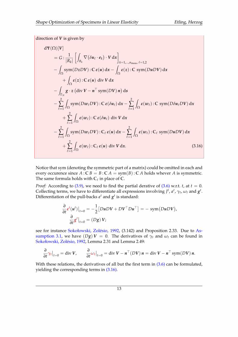
Theorem 3.3. Suppose that u, δu1 and δu2 are the solutions of the forward and sensi-tivity problems (2.4) and (2.12) on the domain Ω. Moreover, let z, w1 and w2 denotethe solutions to the adjoint equations (3.11) and (3.12), respectively. Let V denote aperturbation field satisfying Assumption 3.1. Then the Eulerian derivative of Ψ in the

12


direction of V is given by

dΨ(Ω)[V ]

= G :1|Rk|

[∫Rk

∇(δu` · ek

)· V dx

]k=1,...,nmeas, `=1,2

−∫

Ωsym(DzDV) : C ε(u)dx−

∫Ω

ε(z) : C sym(DuDV)dx

+∫

Ωε(z) : C ε(u) div V dx

−∫

ΓN

g · z(div V − n> sym(DV) n

)ds

−2

∑`=1

∫Ω

sym(Dw`DV) : C ε(δu`)dx−2

∑`=1

∫Ω

ε(w`) : C sym(Dδu`DV)dx

+2

∑`=1

∫Ω

ε(w`) : C ε(δu`) div V dx

−2

∑`=1

∫Ω

sym(Dw`DV) : C` ε(u)dx−2

∑`=1

∫Ω

ε(w`) : C` sym(DuDV)dx

+2

∑`=1

∫Ω

ε(w`) : C` ε(u) div V dx. (3.16)

Notice that sym (denoting the symmetric part of a matrix) could be omitted in each andevery occurence since A : C B = B : C A = sym(B) : C A holds whever A is symmetric.The same formula holds with C` in place of C.

Proof: According to (3.9), we need to find the partial derative of (3.6) w.r.t. t, at t = 0.Collecting terms, we have to differentiate all expressions involving Jt, εt, γt, ωt and gt.Differentiation of the pull-backs εt and gt is standard:

∂

∂tεt(ut)

∣∣t=0 = −1

2[DuDV + DV>Du>

]= − sym

(DuDV

),

∂

∂tgt∣∣

t=0 = (Dg)V ;

see for instance Sokołowski, Zolésio, 1992, (3.142) and Proposition 2.33. Due to As-sumption 3.1, we have (Dg)V = 0. The derivatives of γt and ωt can be found inSokołowski, Zolésio, 1992, Lemma 2.31 and Lemma 2.49:

∂

∂tγt∣∣t=0 = div V ,

∂

∂tωt∣∣t=0 = div V − n>(DV) n = div V − n> sym(DV) n.

With these relations, the derivatives of all but the first term in (3.6) can be formulated,yielding the corresponding terms in (3.16).

13


It remains to differentiate the pulled-back objective 12 trace C(Jt(Ω; δut)), where C(·)

was defined in (3.3). Proceeding as in the proof of Proposition 3.2, we can find

∂

∂t12

trace C(

Jt(Ω; δut))∣∣

t=0 = G :∂

∂t

[Jt(Ω; δut)

]t=0

(3.17)

with G from (3.10). It remains to evaluate the derivative of Jt. We address a singlecomponent of this expression; see (3.8):[ ∂

∂tJtk,`(Ω; δut)

]t=0

=∂

∂t

[1|Rk|

∫T−1

t (Rk)δut

` · ek γt dx]

t=0

=1|Rk|

[∫Rk

δu` · ek div V dx−∫

∂Rk

δu` · ek(V · n

)ds]

=1|Rk|

[∫Rk

∇(δu` · ek

)· V dx

].

The second equality above follows from ∂∂t γt

∣∣t=0 = div V and Sokołowski, Zolésio,

1992, Proposition 2.46. Notice that we are using the inverse transformation T−1t here,

and therefore the sign of V changes compared to Sokołowski, Zolésio, 1992, (2.114). Thethird equality is a consequence of the divergence theorem. Plugging this derivative into(3.17) concludes the proof.

For convenience Table 3.1 summarizes all quantities required for the evaluation of theEulerian derivative (3.16) of the OED objective. An evaluation of the Jacobian, asneeded for efficient least-squares estimation procedures on a given domain Ω as wellas for the evaluation of the OED objective, requires three elasticity solves. Three moreelasticity solves for the adjoint states are needed to evaluate the Eulerian derivative inarbitrary directions V .

evaluation of the Jacobian J (2.14) evaluation of dΨ(Ω)[V ] (3.16) in thein the parameter identification problem optimum experimental design problem

quantity defined by depends on quantity defined by depends on

u (2.4) — w` (3.12) u, δu (via G)δu` (2.12) u z (3.11) w`

Table 3.1: Quantities required to evaluate the Jacobian (left) of the residuals in the pa-rameter identification problem, and the Eulerian derivatives (right) of the ob-jective in the optimum experimental design shape optimization problem. Theindex ` = 1, 2 refers to the parameters to be identified.

We remark that the linear elasticity model does not distinguish between tensile andcompression experiments. When g is replaced by −g in (2.2a), the solutions u and δu`

change in sign due to the linearity of the forward and sensitivity problems (2.4) and(2.12). Consequently the Jacobian (2.14) changes sign but the covariance matrix C(p) in(2.16) remains the same.

14


3.2 SHAPE GRADIENT REPRESENTATIONS

The Eulerian derivative (3.16) constitutes a linear functional on the space of admissiblevelocity fields V . By the Hadamard structure theorem the Eulerian derivative can like-wise be represented by a distribution concentrated on the boundary Γ of the domainΩ, which is applied to the normal vector field (V · n)|Γ restricted to the boundary; seeSokołowski, Zolésio, 1992, Theorem 2.27. Indeed, by tedious calculations involving thedivergence theorem, one can obtain the representation

dΨ(Ω)[V ] =∫

Γfree

h (V · n)ds,

where the so-called Hadamard shape gradient h is given by

h =∫

Γfree

[−(Dσ)[n] n− divΓ σ

· z− σΓ : (Dz)

](V · n)ds

+2

∑`=1

∫Γfree

[−(Dτ`)[n] n− divΓ τ`

· δu` − (τ`)Γ : (Dδu`)

](V · n)ds

+2

∑`=1

∫Γfree

ε(w`) : C` ε(u) (V · n)ds. (3.18)

Here σ = C ε(u) and τ` := C ε(w`) are the stress fields for the forward and adjointproblems, ` = 1, 2. Moreover, (Dσ)[n] denotes the directional derivative of σ in thedirection of the outer unit normal vector n on Γ. Furthermore,

σΓ := σ − (σ n) n> = σ (id−n n>) (3.19)

is the (row-wise) tangential component of σ on Γ, and divΓ σ is the (row-wise) tangen-tial divergence of a matrix field σ restricted to the boundary, i.e.,

divΓ σ := div σ − (Dσ)[n] n; (3.20)

see for instance Sokołowski, Zolésio, 1992, Definition 2.52 or Sonntag, Schmidt, Gauger,2016, eq. (8).

Formula (3.18) is presented here for comparison only, and we will continue to workwith (3.16). Notice that (3.18) requires boundary traces of first- and second-order deriva-tives of the forward and adjoint displacements, while the volume representation (3.16)requires only first-order derivatives in the domain. Hence the argument of Hiptmair,Paganini, Sargheini, 2015 applies also here, showing that the volume representation ofthe Eulerian derivative offers better accuracy in finite element computations.

Following Schulz, Siebenborn, Welker, 2016, we proceed by calculating the Riesz rep-resenter of the linear functional (3.16) with respect to an auxiliary linear elasticity innerproduct. That is, we obtain a displacement field U ∈ W := U ∈ H1(Ω; R2) : U =0 on ΓD ∪ ΓN by solving the linear problem∫

Ω

[2 µ0 ε(U) + λ0 trace(ε(U))

]: ε(V)dx = dΨ(Ω)[V ] for all V ∈ W . (3.21)

15


The displacement field U then serves as the deformation field in the domain transfor-mation Tt(x) := x + t U(x) for all x ∈ Ω, and t will be determined by a line searchprocedure. The Lamé parameters (λ0, µ0) and further details will be specified in Sec-tion 4.

3.3 SINGLE PARAMETER IDENTIFICATION

We return to the discussion at the end of Section 2 about the restriction to only oneparameter. We distinguish two cases:

1. When we estimate only the `-th parameter and the other one is known, we replacethe Jacobian by its `-th column, denoted by j`(Ω; δu`). The optimum experimentaldesign problem (3.2) then reduces to

Minimize Ψ(1)` (Ω) :=

(j`(Ω; δu`)

> Σ−1 j`(Ω; δu`))−1

. (3.22)

Equivalently, we might maximize the `-th diagonal entry in the Fisher informa-tion matrix (2.15). The Eulerian derivative pertaining to (3.22) can be expressedsimilarly as in (3.16), with changes in the first term, the adjoints w` and z, and thesums over `. The first term in (3.16) changes to

g(1)` ·1|Rk|

[∫Rk

∇(δu` · ek

)· V dx

]k=1,...,nmeas

with the vector g(1)` defined by

g(1)` := −2 Σ−1 j`(Ω; δu`)C(j`(Ω; δu`))2.

Notice that g(1)` is not identical to the `-th column of G; compare (3.10). The adjointstates w` and z are obtained as the unique solutions in V of∫

Ωε(z) : C ε(v)dx +

∫Ω

ε(w`) : C`ε(v)dx = 0 for all v ∈ V ,∫Ω

ε(w`) : C ε(v)dx + g(1)` · j`(Ω; v) = 0 for all v ∈ V ,

compare (3.11) and (3.12). Notice that only one adjoint state of type w` is required.

Finally, the summation over ` = 1, 2 in (3.16) is omitted.

2. When both parameters are unknown and need to be estimated but we are onlyinterested in the precision of the `-th parameter, the experimental design problem(3.2) reduces to

Minimize Ψ(2)` (Ω) := C(J(Ω; δu))`,` = e>` C(J(Ω; δu)) e`, (3.23)

16


where e` ∈ R2 is the `-th unit vector. Straightforward calculations show that thematrix G involved in the first term of (3.16) has to be replaced by

G(2)` := −2 Σ−1 J(Ω; δu)C(J(Ω; δu)) e` e>` C(J(Ω; δu)).

Its columns g(2)` appear also in the adjoint equations, which now read

∫Ω

ε(z) : C ε(v)dx +2

∑`=1

∫Ω

ε(w`) : C`ε(v)dx = 0 for all v ∈ V ,∫Ω

ε(w`) : C ε(v)dx + g(2)` · j`(Ω; v) = 0 for all v ∈ V .

In this case the summation over ` = 1, 2 in (3.16) remains.

3.4 STRESS AND PERIMETER PENALTY TERMS

The OED shape optimization problem (3.2) discussed so far suffers from one apparentflaw. Roughly speaking, for any prescribed value of the boundary stress σn = g on ΓN ,a thinning of the specimen will lead to an increase in displacement values u, and thusto a better informed experiment since the sensitivity values δu` will increase as well;see (2.12). One possible remedy would be to assume that the measurements’ standarddeviations σk scale with the measurements and thus with the displacement u. Thisamounts to a constant relative measurement accuracy and it would lead to an additionaldependency of Σ and thus of the estimator covariance matrix C = (J>Σ−1 J)−1 and theobjective (3.2) on the domain Ω. Since constant absolute variance optical measurementsare not unrealistic for our setting, we do not pursue this further. By contrast, we willprevent excessive specimen thinning by adding the stress penalty term

Pσ(Ω; u) :=∫

Ωmax0, |σD

ps|F − σmax2 dx (3.24)

to the objective (3.2). This penalty term becomes active whenever the von Mises stress|σD

ps|F exceeds the allowable stress σmax. A proper definition of the von Mises stressrequires that we consider the 3D analog σps of the planar stress tensor σ. To define it,we require the 3D analog of the Lamé coefficients λ and µ in (2.5), which are given by

λ3D = λ +λ2

2µ− λand µ3D = µ, (3.25)

Note that the second Lamé coefficient (shear modulus) µ remains the same. Assumingthe plane-stress situation (where the specimen can move freely in thickness direction),the corresponding 3D strain and stress tensors are given as follows,

εps(u) :=

ε(u)00

0 0 ε33(u)

and σps := C3D εps =

∗ ∗ 0∗ ∗ 00 0 0

,

17


where ε33(u) := −λ3D trace(ε(u))2µ+λ3D . Equivalently to (2.5), we have

σps = C3Dεps = 2 µ εps + λ3D trace(εps) id3×3, (3.26)

and the positivity requirement λ + µ > 0 translates into 3 λ3D + 2 µ > 0. Notice thatthe above formula for ε33 is easily obtained by the plane-stress assumption (σps)33 = 0.Finally σD

ps := σps − 13 trace(σps) id3×3 is the deviatoric component of the 3D plane-

stress state and |σDps|F is its Frobenius norm.

This explains the composition of the stress penalty (3.24). In our experiments, we alsoadded a standard perimeter penalty

PΓ(Ω) :=∫

Γfree

ds, (3.27)

which helps smooth the boundary and is beneficial with a view towards producibilityof the specimen.

In place of (3.2) we consider from now on the more general problem

Minimize Ψ(Ω) := ψA(C(J(Ω; δu))

)+ ασPσ(Ω; u) + αΓPΓ(Ω), (3.28)

where ασ ≥ 0 and αΓ ≥ 0 are the penalty parameters. Let us briefly discuss the im-plications of the two additional terms. On the perturbed domain Ωt the stress penaltyreads

Pσ,t(Ωt; ut) :=∫

Ωt

max0, |σDps,t|F − σmax2 dx.

Its pull-back to Ω is

P tσ(Ω; u) =

∫Ω

max0, |σD,tps |F − σmax2 γt dx, (3.29)

where

σtps = C3Dεt

ps(ut) = C3D

εt(ut)00

0 0 −λ3D trace(εt(ut))2µ+λ3D

and σD,tps = [σt

ps]D

holds with εt(ut) from (3.7). The term (3.29) is added to the Lagrangian (3.6). Its differ-entiation at t = 0 w.r.t. u in the direction of v gives us an additional term which appearsin the “right hand side” of the adjoint equation (3.11) for z. The latter is thus replacedby

∫Ω

ε(z) : C ε(v)dx +2

∑`=1

∫Ω

ε(w`) : C`ε(v)dx

+ 2 ασ

∫Ω

max0, |σDps|F − σmax

σDps

|σDps|F

: σDps(ε(v)

)dx = 0 for all v ∈ V . (3.30)

18


The adjoints w` (` = 1, 2) remain unchanged; see (3.12).

We proceed similarly for the perimeter penalty (3.27), whose pull-back is given by

P tΓ(Ω) :=

∫Γfree

ωt ds. (3.31)

Since it does not depend on state variables, no further changes to the adjoint equationsare necessary. By adding the partial derivatives of (3.29) and (3.31) w.r.t. t at t = 0 to(3.16) we obtain the Eulerian shape derivative for the penalized problem (3.28) as statedin the following theorem. The details are left to the reader.

Theorem 3.4. Suppose that u, δu1 and δu2 are the solutions of the forward and sensi-tivity problems (2.4) and (2.12) on the domain Ω. Moreover, let z, w1 and w2 denotethe solutions to the adjoint equations (3.30) and (3.12), respectively. Let V denote aperturbation field satisfying Assumption 3.1. Then the Eulerian derivative of Ψ in thedirection of V is given by

dΨ(Ω)[V ] = formula (3.16)

− 2 ασ

∫Ω

max0, |σDps|F − σmax

σDps

|σDps|F

: σDps(sym(DuDV)

)dx

+ ασ

∫Ω

max0, |σDps|F − σmax2 div V dx

+ αΓ

∫Γfree

(div V − n> sym(DV) n

)ds. (3.32)

4 NUMERICAL EXPERIMENTS

In this section we describe a number of numerical experiments based on the setup de-scribed in Figure 2.1 and Figure 3.1. As mentioned earlier, the elasticity parameters willbe considered fixed since we are mainly interested in solving the OED problem.

We choose nominal parameters

λ = 943 N/mm2, µ = 803 N/mm2, (4.1)

which corresponds to a certain polycarbonate with elasticity modulus and Poisson ratioE3D = 2200 N/mm2 and ν3D = 0.37 or equivalently, Lamé parameters

λ3D =E3D ν3D

(1 + ν3D)(1− 2 ν3D)= 2285 N/mm2, µ3D =

E3D

2 (1 + ν3D)= 803 N/mm2.

(4.2)The relationship between the 2D and 3D Lamé parameters was described in the trans-formation formula (3.25). To obtain a consistent set of dimensions, all lengths will be

19


measured in mm. All measurements are assumed to have identical standard deviationσk ≡ σ = 0.1 mm.

All elasticity problems (see Table 3.1) were discretized using P2 (piecewise quadratic,continuous) finite elements on triangular meshes in 2D. Consequently, the stresses suchas σ = C ε(u) are piecewise linear functions.

In all of our case studies, we consider a symmetric situation with a horizontal symmetryaxis Γsymmetry, and only the upper half of the domain is involved in the calculations andwill be displayed. The boundary conditions along the symmetry axis are e>1 σ n = 0and e>2 u = 0, and likewise for the sensitivity and adjoint equations.

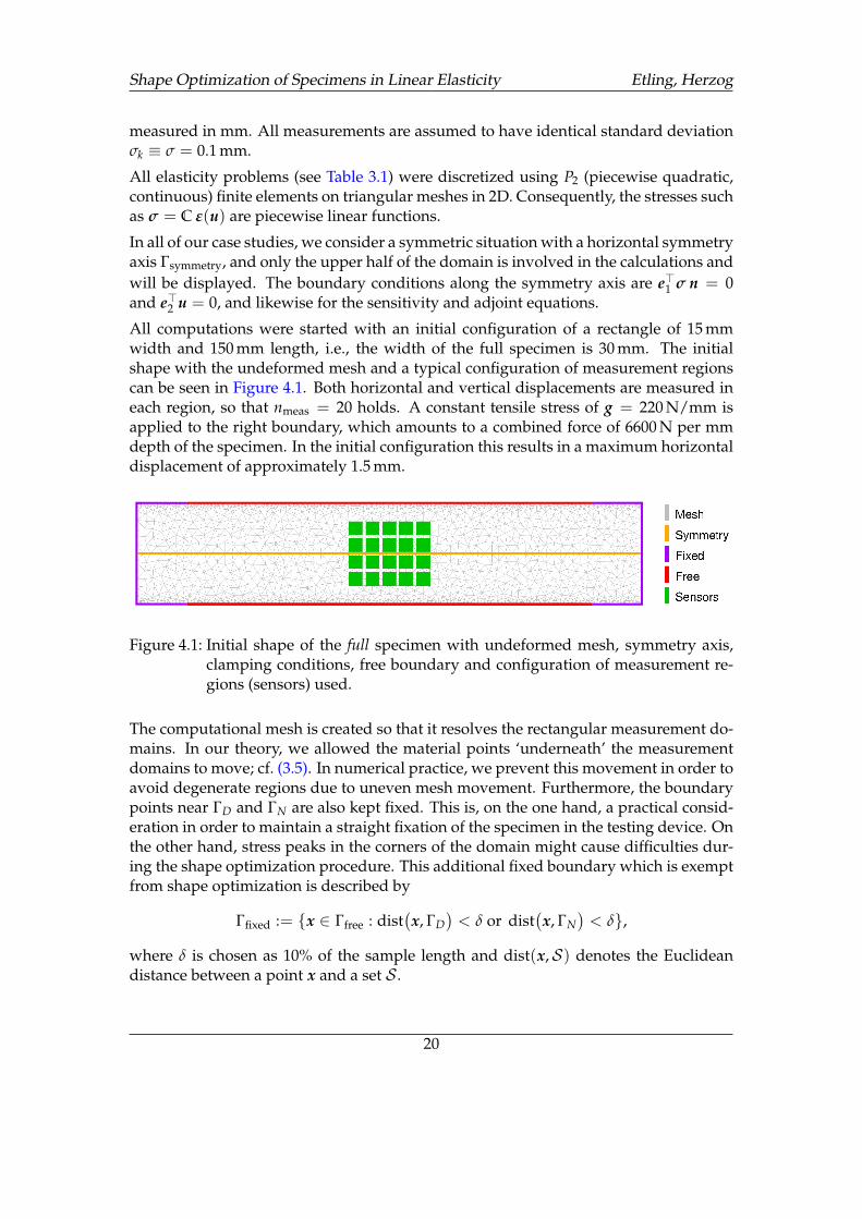
All computations were started with an initial configuration of a rectangle of 15 mmwidth and 150 mm length, i.e., the width of the full specimen is 30 mm. The initialshape with the undeformed mesh and a typical configuration of measurement regionscan be seen in Figure 4.1. Both horizontal and vertical displacements are measured ineach region, so that nmeas = 20 holds. A constant tensile stress of g = 220 N/mm isapplied to the right boundary, which amounts to a combined force of 6600 N per mmdepth of the specimen. In the initial configuration this results in a maximum horizontaldisplacement of approximately 1.5 mm.

Figure 4.1: Initial shape of the full specimen with undeformed mesh, symmetry axis,clamping conditions, free boundary and configuration of measurement re-gions (sensors) used.

The computational mesh is created so that it resolves the rectangular measurement do-mains. In our theory, we allowed the material points ‘underneath’ the measurementdomains to move; cf. (3.5). In numerical practice, we prevent this movement in order toavoid degenerate regions due to uneven mesh movement. Furthermore, the boundarypoints near ΓD and ΓN are also kept fixed. This is, on the one hand, a practical consid-eration in order to maintain a straight fixation of the specimen in the testing device. Onthe other hand, stress peaks in the corners of the domain might cause difficulties dur-ing the shape optimization procedure. This additional fixed boundary which is exemptfrom shape optimization is described by

Γfixed := x ∈ Γfree : dist(x, ΓD

)< δ or dist

(x, ΓN

)< δ,

where δ is chosen as 10% of the sample length and dist(x,S) denotes the Euclideandistance between a point x and a set S .

20


Fixing the measurement regions as well as the holding fixture are easily achieved byrestricting the deformation spaceW for the auxiliary elasticity problem (3.21) to

W := U ∈ H1(Ω; R2) : U = 0 on ΓD ∪ ΓN ∪ Γfixed ∪ Γsymmetry

and on cl Rk for k = 1, . . . , nmeas.

Here cl Rk denotes the closure of Rk. The measurement subdomains as well as the inertboundary ΓD ∪ ΓN ∪ Γfixed ∪ Γsymmetry are denoted by Sensors (green) and Fixed (violet) inFigure 4.1. Taking into account the addition of the two penalty terms of the objective asdiscussed in Section 3.4, the auxiliary elasticity problem to obtain the Riesz representerof the Eulerian shape derivative amounts to finding the displacement field U ∈ W suchthat ∫

Ω

[2 µ0 ε(U) + λ0 trace(ε(U))

]: ε(V)dx = dΨ(Ω)[V ] for all V ∈ W . (4.3)

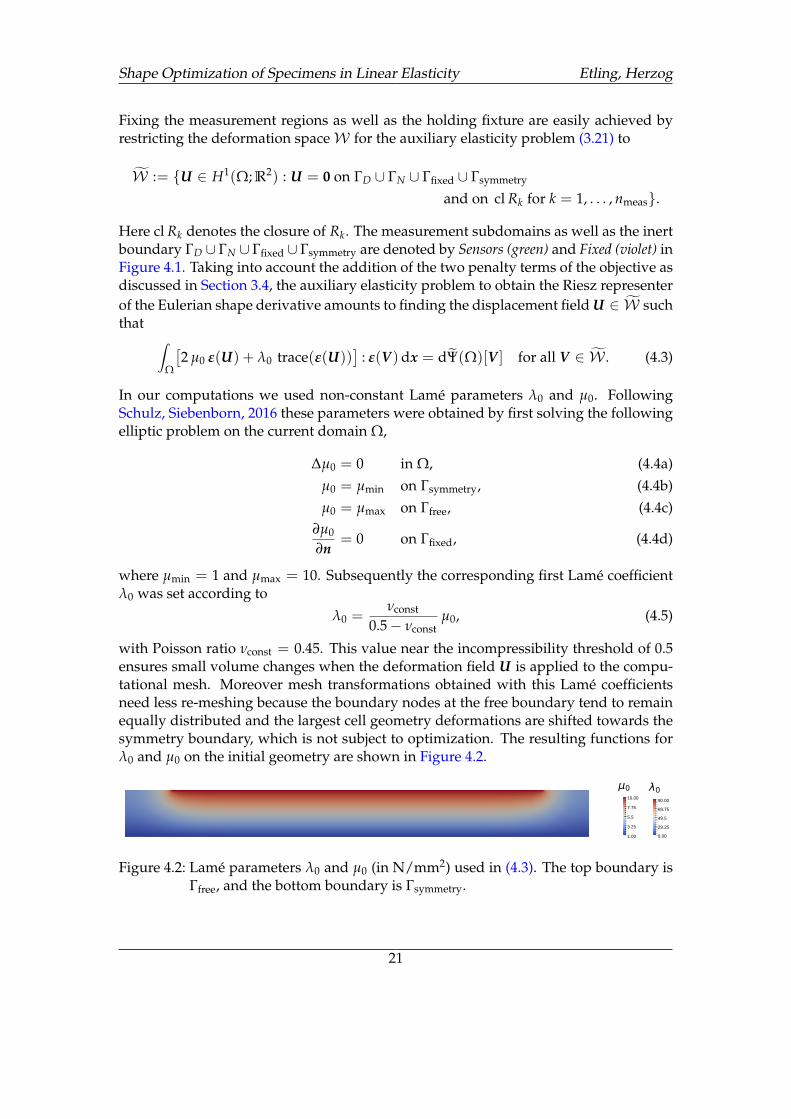
In our computations we used non-constant Lamé parameters λ0 and µ0. FollowingSchulz, Siebenborn, 2016 these parameters were obtained by first solving the followingelliptic problem on the current domain Ω,

∆µ0 = 0 in Ω, (4.4a)µ0 = µmin on Γsymmetry, (4.4b)µ0 = µmax on Γfree, (4.4c)

∂µ0

∂n= 0 on Γfixed, (4.4d)

where µmin = 1 and µmax = 10. Subsequently the corresponding first Lamé coefficientλ0 was set according to

λ0 =νconst

0.5− νconstµ0, (4.5)

with Poisson ratio νconst = 0.45. This value near the incompressibility threshold of 0.5ensures small volume changes when the deformation field U is applied to the compu-tational mesh. Moreover mesh transformations obtained with this Lamé coefficientsneed less re-meshing because the boundary nodes at the free boundary tend to remainequally distributed and the largest cell geometry deformations are shifted towards thesymmetry boundary, which is not subject to optimization. The resulting functions forλ0 and µ0 on the initial geometry are shown in Figure 4.2.

29.25

49.5

69.75

9.00

90.00

3.25

5.5

7.75

1.00

10.00

Figure 4.2: Lamé parameters λ0 and µ0 (in N/mm2) used in (4.3). The top boundary isΓfree, and the bottom boundary is Γsymmetry.

21


We followed an optimize–then discretize approach and implemented a gradient de-scent method to optimize the specimen shape according to the shape optimizationproblem (3.2). The deformation field U from (4.3) serves as the descent direction and itgenerates the transformation Tt = id+t U which is applied to the computational meshrepresenting the current domain Ω. The parameter t > 0 is obtained via an Armijobacktracking line search; see for instance Nocedal, Wright, 2006, Algorithm 3.1. Thetrial step size t is accepted if

Ψ(Tt(Ω)) ≤ Ψ(Ω) + t σ dΨ(Ω)[U],

holds with σ = 0.01. When a step is rejected the step size t is reduced to β t with β = 0.5.The gradient descent method was stopped as soon as the relative stopping criterion

Ψ(Tt(Ω))− Ψ(Ω)

Ψ(Ω)≤ ε (4.6)

was satisfied.Our algorithm observes the mesh quality in terms of the aspect ratio (the ratio of thediameters of inscribed and circumscribed circles, times the cell dimension) of everycell. Re-meshing is triggered as soon as an element has an aspect ratio lower than 0.1at the end of a gradient descent step. During re-meshing the measurement domainsare preserved but additional boundary nodes may be added between existing ones incase boundary nodes become unevenly spaced. Additional boundary nodes are placedbased on linear interpolation. The occurence of re-meshing will be indicated in thenumerical results.Finally our method monitors the three contributions to the objective (3.28) individually.In case the combined penalty terms increase significantly from one iteration to the next,the accepted Armijo step size is reduced as a precaution to avoid irregularities in thefree boundary part of the mesh. This typically occurs only in the initial iterations andcan be seen at the beginning of the step size plot in Figure 4.4.All computations were implemented in the finite element toolbox FENICS (version2017.1); see Logg, Mardal, Wells, 2012 . In the remainder of this section we describenumerical experiments and results for three different settings. In the first setting (Sec-tion 4.1) we consider the case where both Lamé coefficients (λ, µ) are to be identified.In Section 4.2 we focus on the two single-parameter cases of type 1 as described Sec-tion 3.3, i.e., only one of the Lamé parameters needs to be estimated. Table 4.1 showsthe values of the penalty parameters (ασ , αΓ) as well as the tolerance ε in the stoppingcriterion (4.6) which are in effect in each case. The maximal allowable stress was set toσmax = 52 N/mm2 in each case. For comparison, the yield stress of polycarbonate isdescribed in the literature to lie between 55 N/mm2 and 75 N/mm2.

4.1 EXPERIMENT 1: JOINT PARAMETER IDENTIFICATION

In this first experiment we consider the OED shape optimization problem for the casewhen both Lamé parameters (λ, µ) in (2.5) are to be identified from a single experiment.

22


section parameters ασ αΓ ε

Section 4.1 (λ, µ) 5e1 2e4 1e−5Section 4.2 λ 1e2 5e2 1e−5Section 4.2 µ 5e−2 1e1 1e−5

Table 4.1: Penalty parameters (ασ , αΓ) and the stopping tolerance ε used for the casestudies in this section.

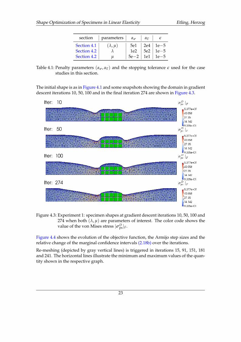
The initial shape is as in Figure 4.1 and some snapshots showing the domain in gradientdescent iterations 10, 50, 100 and in the final iteration 274 are shown in Figure 4.3.

Figure 4.3: Experiment 1: specimen shapes at gradient descent iterations 10, 50, 100 and274 when both (λ, µ) are parameters of interest. The color code shows thevalue of the von Mises stress |σD

ps|F.

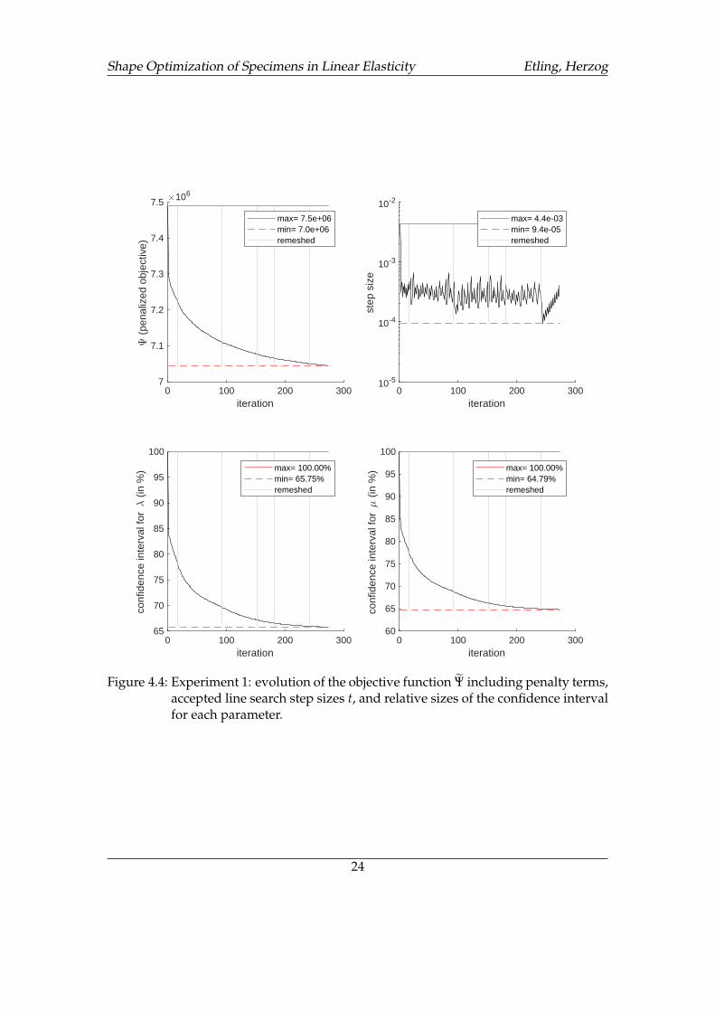
Figure 4.4 shows the evolution of the objective function, the Armijo step sizes and therelative change of the marginal confidence intervals (2.18b) over the iterations.

Re-meshing (depicted by gray vertical lines) is triggered in iterations 15, 91, 151, 181and 241. The horizontal lines illustrate the minimum and maximum values of the quan-tity shown in the respective graph.

23


0 100 200 300iteration

7

7.1

7.2

7.3

7.4

7.5

(pe

naliz

ed o

bjec

tive)

106

max= 7.5e+06min= 7.0e+06remeshed


10-5

10-4

10-3

10-2

step

siz

e

max= 4.4e-03min= 9.4e-05remeshed


65

70

75

80

85

90

95

100

conf

iden

ce in

terv

al fo

r (

in %

) max= 100.00%min= 65.75%remeshed


60

65

70

75

80

85

90

95

100

conf

iden

ce in

terv

al fo

r (

in %

) max= 100.00%min= 64.79%remeshed

Figure 4.4: Experiment 1: evolution of the objective function Ψ including penalty terms,accepted line search step sizes t, and relative sizes of the confidence intervalfor each parameter.

24


4.2 EXPERIMENT 2: SINGLE PARAMETER IDENTIFICATION

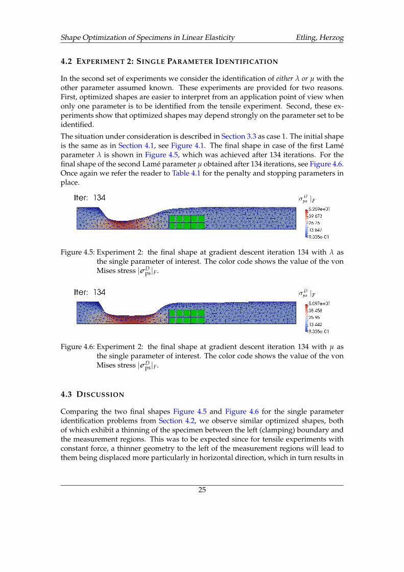
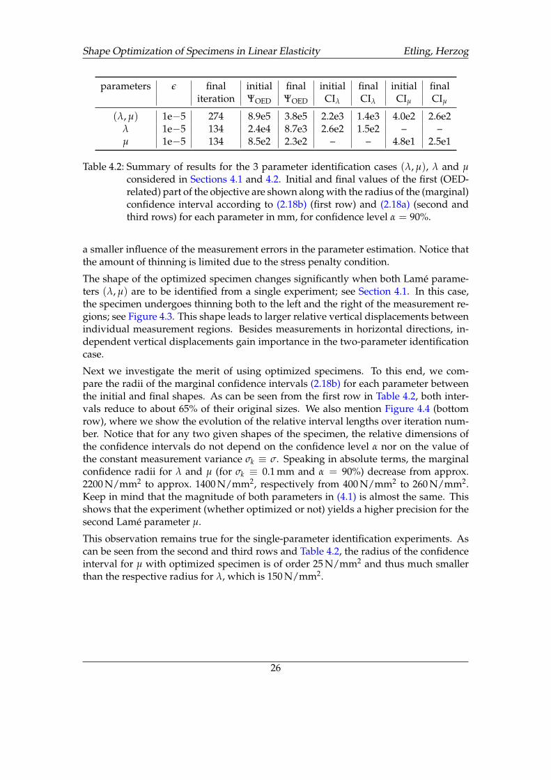
In the second set of experiments we consider the identification of either λ or µ with theother parameter assumed known. These experiments are provided for two reasons.First, optimized shapes are easier to interpret from an application point of view whenonly one parameter is to be identified from the tensile experiment. Second, these ex-periments show that optimized shapes may depend strongly on the parameter set to beidentified.

The situation under consideration is described in Section 3.3 as case 1. The initial shapeis the same as in Section 4.1, see Figure 4.1. The final shape in case of the first Laméparameter λ is shown in Figure 4.5, which was achieved after 134 iterations. For thefinal shape of the second Lamé parameter µ obtained after 134 iterations, see Figure 4.6.Once again we refer the reader to Table 4.1 for the penalty and stopping parameters inplace.

Figure 4.5: Experiment 2: the final shape at gradient descent iteration 134 with λ asthe single parameter of interest. The color code shows the value of the vonMises stress |σD

ps|F.

Figure 4.6: Experiment 2: the final shape at gradient descent iteration 134 with µ asthe single parameter of interest. The color code shows the value of the vonMises stress |σD

ps|F.

4.3 DISCUSSION

Comparing the two final shapes Figure 4.5 and Figure 4.6 for the single parameteridentification problems from Section 4.2, we observe similar optimized shapes, bothof which exhibit a thinning of the specimen between the left (clamping) boundary andthe measurement regions. This was to be expected since for tensile experiments withconstant force, a thinner geometry to the left of the measurement regions will lead tothem being displaced more particularly in horizontal direction, which in turn results in

25


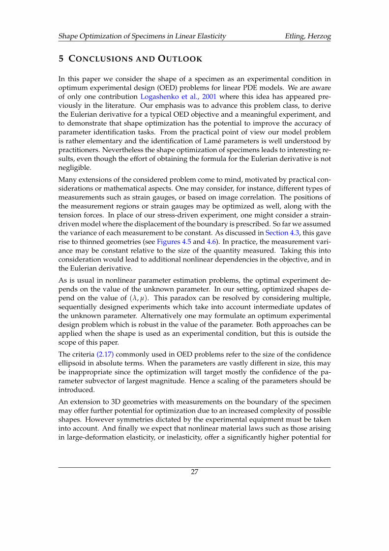
parameters ε final initial final initial final initial finaliteration ΨOED ΨOED CIλ CIλ CIµ CIµ

(λ, µ) 1e−5 274 8.9e5 3.8e5 2.2e3 1.4e3 4.0e2 2.6e2λ 1e−5 134 2.4e4 8.7e3 2.6e2 1.5e2 – –µ 1e−5 134 8.5e2 2.3e2 – – 4.8e1 2.5e1

Table 4.2: Summary of results for the 3 parameter identification cases (λ, µ), λ and µconsidered in Sections 4.1 and 4.2. Initial and final values of the first (OED-related) part of the objective are shown along with the radius of the (marginal)confidence interval according to (2.18b) (first row) and (2.18a) (second andthird rows) for each parameter in mm, for confidence level α = 90%.

a smaller influence of the measurement errors in the parameter estimation. Notice thatthe amount of thinning is limited due to the stress penalty condition.

The shape of the optimized specimen changes significantly when both Lamé parame-ters (λ, µ) are to be identified from a single experiment; see Section 4.1. In this case,the specimen undergoes thinning both to the left and the right of the measurement re-gions; see Figure 4.3. This shape leads to larger relative vertical displacements betweenindividual measurement regions. Besides measurements in horizontal directions, in-dependent vertical displacements gain importance in the two-parameter identificationcase.

Next we investigate the merit of using optimized specimens. To this end, we com-pare the radii of the marginal confidence intervals (2.18b) for each parameter betweenthe initial and final shapes. As can be seen from the first row in Table 4.2, both inter-vals reduce to about 65% of their original sizes. We also mention Figure 4.4 (bottomrow), where we show the evolution of the relative interval lengths over iteration num-ber. Notice that for any two given shapes of the specimen, the relative dimensions ofthe confidence intervals do not depend on the confidence level α nor on the value ofthe constant measurement variance σk ≡ σ. Speaking in absolute terms, the marginalconfidence radii for λ and µ (for σk ≡ 0.1 mm and α = 90%) decrease from approx.2200 N/mm2 to approx. 1400 N/mm2, respectively from 400 N/mm2 to 260 N/mm2.Keep in mind that the magnitude of both parameters in (4.1) is almost the same. Thisshows that the experiment (whether optimized or not) yields a higher precision for thesecond Lamé parameter µ.

This observation remains true for the single-parameter identification experiments. Ascan be seen from the second and third rows and Table 4.2, the radius of the confidenceinterval for µ with optimized specimen is of order 25 N/mm2 and thus much smallerthan the respective radius for λ, which is 150 N/mm2.

26


5 CONCLUSIONS AND OUTLOOK

In this paper we consider the shape of a specimen as an experimental condition inoptimum experimental design (OED) problems for linear PDE models. We are awareof only one contribution Logashenko et al., 2001 where this idea has appeared pre-viously in the literature. Our emphasis was to advance this problem class, to derivethe Eulerian derivative for a typical OED objective and a meaningful experiment, andto demonstrate that shape optimization has the potential to improve the accuracy ofparameter identification tasks. From the practical point of view our model problemis rather elementary and the identification of Lamé parameters is well understood bypractitioners. Nevertheless the shape optimization of specimens leads to interesting re-sults, even though the effort of obtaining the formula for the Eulerian derivative is notnegligible.

Many extensions of the considered problem come to mind, motivated by practical con-siderations or mathematical aspects. One may consider, for instance, different types ofmeasurements such as strain gauges, or based on image correlation. The positions ofthe measurement regions or strain gauges may be optimized as well, along with thetension forces. In place of our stress-driven experiment, one might consider a strain-driven model where the displacement of the boundary is prescribed. So far we assumedthe variance of each measurement to be constant. As discussed in Section 4.3, this gaverise to thinned geometries (see Figures 4.5 and 4.6). In practice, the measurement vari-ance may be constant relative to the size of the quantity measured. Taking this intoconsideration would lead to additional nonlinear dependencies in the objective, and inthe Eulerian derivative.

As is usual in nonlinear parameter estimation problems, the optimal experiment de-pends on the value of the unknown parameter. In our setting, optimized shapes de-pend on the value of (λ, µ). This paradox can be resolved by considering multiple,sequentially designed experiments which take into account intermediate updates ofthe unknown parameter. Alternatively one may formulate an optimum experimentaldesign problem which is robust in the value of the parameter. Both approaches can beapplied when the shape is used as an experimental condition, but this is outside thescope of this paper.

The criteria (2.17) commonly used in OED problems refer to the size of the confidenceellipsoid in absolute terms. When the parameters are vastly different in size, this maybe inappropriate since the optimization will target mostly the confidence of the pa-rameter subvector of largest magnitude. Hence a scaling of the parameters should beintroduced.

An extension to 3D geometries with measurements on the boundary of the specimenmay offer further potential for optimization due to an increased complexity of possibleshapes. However symmetries dictated by the experimental equipment must be takeninto account. And finally we expect that nonlinear material laws such as those arisingin large-deformation elasticity, or inelasticity, offer a significantly higher potential for

27


OED techniques since in this realm meaningful experiments can be intricate and lessobvious to practitioners. The techniques developed in this paper can be extended tosuch nonlinear PDEs models. This will incur, besides analytical challenges, furtherdependencies in the forward, sensitivity and adjoint equations. The details are left forfuture research.

ACKNOWLEDGMENTS

The authors would like to thank Gerd Wachsmuth for fruitful discussions and FelixOspald for help with the FENICS implementation.

REFERENCES

Bambach, M.; Heinkenschloss, M.; Herty, M. (2013). “A method for model identificationand parameter estimation”. Inverse Problems 29.2, pp. 025009, 19. ISSN: 0266-5611. DOI:10.1088/0266-5611/29/2/025009.

Bock, Hans Georg; Körkel, Stefan; Schlöder, Johannes P. (2013). “Parameter estimationand optimum experimental design for differential equation models”. Model based pa-rameter estimation. Vol. 4. Contributions in Mathematical and Computational Sciences.Heidelberg: Springer, pp. 1–30. DOI: 10.1007/978-3-642-30367-8 1.

Bonnet, Marc; Constantinescu, Andrei (2005). “Inverse problems in elasticity”. InverseProblems 21.2, R1–R50. ISSN: 0266-5611. DOI: 10.1088/0266-5611/21/2/R01.

Carraro, Thomas (2005). “Parameter estimation and optimal experimental design inflow reactors”. http://nbn-resolving.de/urn/resolver.pl?urn=urn:nbn:de:bsz:16-opus-61141. PhD thesis. University of Heidelberg.

Céa, Jean (1986). “Conception optimale ou identification de formes: calcul rapide de ladérivée directionnelle de la fonction coût”. RAIRO Modélisation Mathématique et Anal-yse Numérique 20.3, pp. 371–402. ISSN: 0764-583X. DOI: 10.1051/m2an/1986200303711.

Davis, J.R. (2004). Tensile Testing. 2nd ed. ASM International.Delfour, M. C.; Zolésio, J.-P. (1988). “Shape sensitivity analysis via min max differentia-

bility”. SIAM Journal on Control and Optimization 26.4, pp. 834–862. ISSN: 0363-0129.DOI: 10.1137/0326048.

Eppler, K. (2010). On Hadamard Shape Gradient Representations in Linear Elasticity. Tech.rep. SPP1253-104. Priority Program 1253, German Research Foundation.

Fedorov, Valerii V.; Leonov, Sergei L. (2014). Optimal design for nonlinear response models.Chapman & Hall/CRC Biostatistics Series. Boca Raton, FL: CRC Press, pp. xxviii+373.ISBN: 978-1-4398-2151-0.

Haber, E.; Horesh, L.; Tenorio, L. (2008). “Numerical methods for experimental designof large-scale linear ill-posed inverse problems”. Inverse Problems 24.5, pp. 055012, 17.ISSN: 0266-5611. DOI: 10.1088/0266-5611/24/5/055012.

Herzog, R.; Riedel, I. (2015). “Sequentially Optimal Sensor Placement in ThermoelasticModels for Real Time Applications”. Optimization and Engineering 16.4, pp. 737–766.DOI: 10.1007/s11081-015-9275-0.

28

http://dx.doi.org/10.1088/0266-5611/29/2/025009

http://dx.doi.org/10.1007/978-3-642-30367-8_1

http://dx.doi.org/10.1088/0266-5611/21/2/R01

http://nbn-resolving.de/urn/resolver.pl?urn=urn:nbn:de:bsz:16-opus-61141

http://nbn-resolving.de/urn/resolver.pl?urn=urn:nbn:de:bsz:16-opus-61141

http://dx.doi.org/10.1051/m2an/1986200303711

http://dx.doi.org/10.1137/0326048

http://dx.doi.org/10.1088/0266-5611/24/5/055012

http://dx.doi.org/10.1007/s11081-015-9275-0


Herzog, Roland; Ospald, Felix (2017). “Parameter Identification for Short Fiber-ReinforcedPlastics using Optimal Experimental Design”. International Journal for Numerical Meth-ods in Engineering 110.8, pp. 703–725. ISSN: 1097-0207. DOI: 10.1002/nme.5371.

Hiptmair, R.; Paganini, A.; Sargheini, S. (2015). “Comparison of approximate shape gra-dients”. BIT. Numerical Mathematics 55.2, pp. 459–485. ISSN: 0006-3835. DOI: 10.1007/s10543-014-0515-z.

Ito, Kazufumi; Kunisch, Karl (1995). “Maximizing robustness in nonlinear ill-posed in-verse problems”. SIAM Journal on Control and Optimization 33.2, pp. 643–666. ISSN:0363-0129. DOI: 10.1137/S0363012992230982.

Körkel, S; Bauer, Irene; Bock, Hans Georg; Schlöder, JP (1999). “A sequential approachfor nonlinear optimum experimental design in DAE systems”. Scientific Computing inChemical Engineering II. Vol. 2. Springer-Verlag, pp. 338–345.

Körkel, Stefan; Kostina, Ekaterina; Bock, Hans Georg; Schlöder, Johannes P. (2004).“Numerical methods for optimal control problems in design of robust optimal ex-periments for nonlinear dynamic processes”. Optimization Methods & Software 19.3-4.The First International Conference on Optimization Methods and Software. Part II,pp. 327–338. ISSN: 1055-6788. DOI: 10.1080/10556780410001683078.

Lahmer, T.; Kaltenbacher, B.; Schulz, V. (2008). “Optimal measurement selection forpiezoelectric material tensor identification”. Inverse Problems in Science and Engineer-ing 16.3, pp. 369–387. ISSN: 1741-5977. DOI: 10.1080/17415970701743368.

Laurain, A.; Sturm, K. (2016). “Distributed shape derivative via averaged adjoint methodand applications”. ESAIM. Mathematical Modelling and Numerical Analysis 50.4, pp. 1241–1267. DOI: 10.1051/m2an/2015075.

Logashenko, Dmitriy; Maar, Bernd; Schulz, Volker; Wittum, Gabriel (2001). “Optimalgeometrical design of Bingham parameter measurement devices”. Fast solution of dis-cretized optimization problems (Berlin, 2000). Vol. 138. International Series of NumericalMathematics. Basel: Birkhäuser, pp. 167–183.

Logg, Anders; Mardal, Kent-Andre; Wells, Garth N., et al. (2012). Automated Solution ofDifferential Equations by the Finite Element Method. Springer. ISBN: 978-3-642-23098-1.DOI: 10.1007/978-3-642-23099-8.

Nocedal, J.; Wright, S. (2006). Numerical Optimization. Second. New York: Springer. DOI:10.1007/978-0-387-40065-5.

Pronzato, Luc; Pázman, Andrej (2013). Design of experiments in nonlinear models. Vol. 212.Lecture Notes in Statistics. Asymptotic normality, optimality criteria and small-sampleproperties. Springer, New York, pp. xvi+399. ISBN: 978-1-4614-6362-7. DOI: 10.1007/978-1-4614-6363-4.

Pukelsheim, F. (2006). Optimal design of experiments. Vol. 50. Classics in Applied Math-ematics. Reprint of the 1993 original. Philadelphia, PA: Society for Industrial andApplied Mathematics (SIAM), pp. xxxii+454. ISBN: 0-89871-604-7.

Schulz, Volker H.; Siebenborn, Martin; Welker, Kathrin (2016). “Efficient PDE constrainedshape optimization based on Steklov-Poincaré type metrics”. SIAM Journal on Opti-mization 26.4, pp. 2800–2819.

29

http://dx.doi.org/10.1002/nme.5371

http://dx.doi.org/10.1007/s10543-014-0515-z

http://dx.doi.org/10.1007/s10543-014-0515-z

http://dx.doi.org/10.1137/S0363012992230982

http://dx.doi.org/10.1080/10556780410001683078

http://dx.doi.org/10.1080/17415970701743368

http://dx.doi.org/10.1051/m2an/2015075

http://dx.doi.org/10.1007/978-3-642-23099-8

http://dx.doi.org/10.1007/978-0-387-40065-5

http://dx.doi.org/10.1007/978-1-4614-6363-4

http://dx.doi.org/10.1007/978-1-4614-6363-4


Schulz, Volker; Siebenborn, Martin (2016). “Computational comparison of surface met-rics for PDE constrained shape optimization”. Computational Methods in Applied Math-ematics 16.3, pp. 485–496. ISSN: 1609-4840. DOI: 10.1515/cmam-2016-0009.

Skanda, D.; Lebiedz, D. (2010). “An optimal experimental design approach to modeldiscrimination in dynamic biochemical systems”. Bioinformatics 26.7, pp. 939–945.DOI: 10.1093/bioinformatics/btq074.

Sokołowski, J.; Zolésio, J.-P. (1992). Introduction to Shape Optimization. New York: Springer.Sonntag, Matthias; Schmidt, Stephan; Gauger, Nicolas R. (2016). “Shape derivatives

for the compressible Navier-Stokes equations in variational form”. Journal of Com-putational and Applied Mathematics 296, pp. 334–351. ISSN: 0377-0427. DOI: 10.1016/j.cam.2015.09.010.

Sturm, K. (2015). “Minimax Lagrangian Approach to the Differentiability of NonlinearPDE Constrained Shape Functions without Saddle Point Assumptions”. SIAM Jour-nal on Control and Optimization 53.4, pp. 2017–2039. DOI: 10.1137/130930807.

Ucinski, Dariusz (2005). Optimal measurement methods for distributed parameter systemidentification. Systems and Control Series. Boca Raton, FL: CRC Press, pp. xviii+371.ISBN: 0-8493-2313-4.

30

http://dx.doi.org/10.1515/cmam-2016-0009

http://dx.doi.org/10.1093/bioinformatics/btq074

http://dx.doi.org/10.1016/j.cam.2015.09.010

http://dx.doi.org/10.1016/j.cam.2015.09.010

http://dx.doi.org/10.1137/130930807

OPTIMUM EXPERIMENTAL DESIGN BY SHAPE OPTIMIZATION … · Shape Optimization of Specimens in Linear...

Documents

Transcript of OPTIMUM EXPERIMENTAL DESIGN BY SHAPE OPTIMIZATION … · Shape Optimization of Specimens in Linear...