Optimizing Product Line Designs: Efficient Methods and ...

Optimizing Product Line Designs: Efficient Methods and Comparisons

February 2005

Alexandre Belloni [email protected]

Robert Freund

[email protected]

Matthew Selove [email protected]

Duncan Simester [email protected]

MIT Sloan School of Management Cambridge MA 02142

We thank Karen Freeman for research assistance on this project and Ely Dahan, John Hauser, and Olivier Toubia for the data used in the study.

Optimizing Product Line Designs: Efficient Methods and Comparisons

We compare a broad range of optimal product line design methods. The comparisons take advantage of recent advances that make it possible to identify the optimal solution to problems that are too large for complete enumeration. Several of the methods perform surprisingly well, including Simulated Annealing, Product-Swapping and Genetic Algorithms. The Product-Swapping heuristic is remarkable for its simplicity. The performance of this heuristic suggests that the optimal product line design problem may be far easier to solve in practice than indicated by complexity theory.

1. Introduction There is an extensive literature investigating how firms can use conjoint measures of

customer preferences to optimize the design of their product lines. The origins of this

literature coincide with the first articles proposing the use of conjoint analysis. In

contrast to conjoint analysis, where there is a growing literature documenting its

measurement value, there is relatively little evidence validating the effectiveness of

product line optimization methods on realistic problems. Previous validations have

focused on small problems for which it is possible to identify the optimal design through

complete enumeration. For larger problems, optimal solutions have been unobtainable,

making it impossible to evaluate whether the methods yield solutions that are close to

optimal. This limitation is important as the methods are designed for these larger

problems in which complete enumeration is not possible. As a result, it has not been

possible to evaluate the methods on the problems for which they were designed.

In this paper we compare the performance of a broad range of optimization methods on a

more realistic product line design problem. The comparisons use conjoint data collected

from real customers describing their preferences for computer laptop bags. We compare

the quality of the solutions, together with the complexity of the methods and the cost of

computation. The comparison is made possible by recent advances in optimization

methods and computer hardware. Using a combination of sophisticated fine-tuned

discrete optimization methods (Lagrangian relaxation with branch and bound), we can

now guarantee optimality in realistic product line design problems that are too large for

complete enumeration.

Several of the methods we test consistently reach optimal solutions, although none of the

methods guarantee the global optimality of their solutions. Even when measurement

errors are introduced, the most successful methods still generate solutions within 3% of

the optimum. These findings indicate that realistic product line design problems are

easier to solve than previously thought. Surprisingly, relatively simple methods are

capable of computing near-optimal solutions with little computational burden.

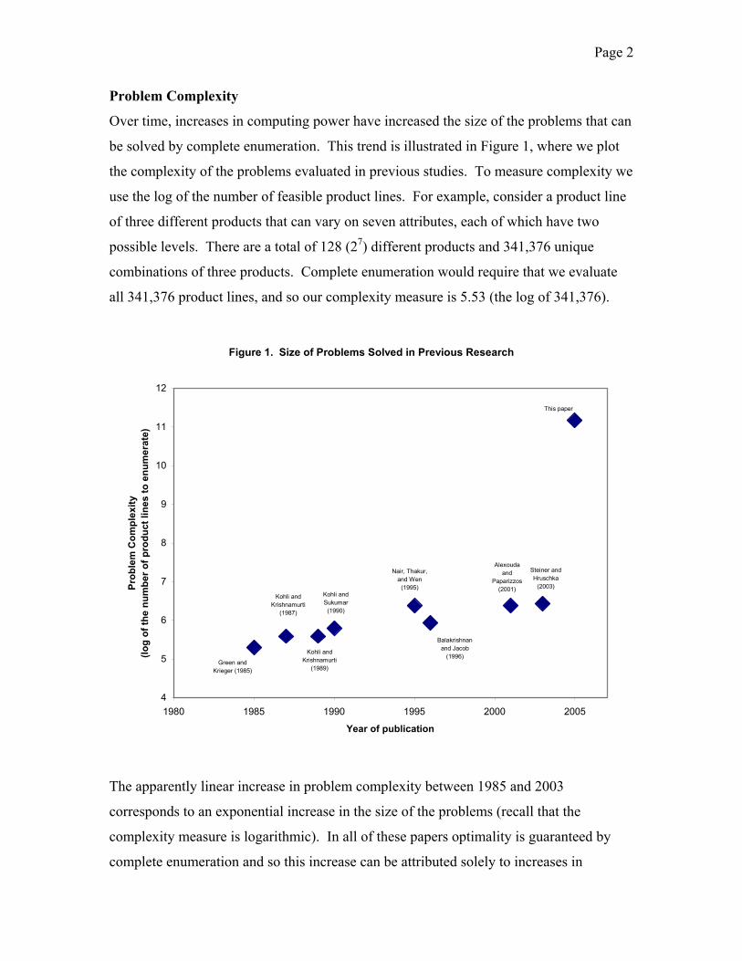
Problem Complexity

Over time, increases in computing power have increased the size of the problems that can

be solved by complete enumeration. This trend is illustrated in Figure 1, where we plot

the complexity of the problems evaluated in previous studies. To measure complexity we

use the log of the number of feasible product lines. For example, consider a product line

of three different products that can vary on seven attributes, each of which have two

possible levels. There are a total of 128 (27) different products and 341,376 unique

combinations of three products. Complete enumeration would require that we evaluate

all 341,376 product lines, and so our complexity measure is 5.53 (the log of 341,376).

Figure 1. Size of Problems Solved in Previous Research

4

5

6

7

8

9

10

11

12

1980 1985 1990 1995 2000 2005

Year of publication

Prob

lem

Com

plex

ity(lo

g of

the

num

ber o

f pro

duct

line

s to

enu

mer

ate)

Green and Krieger (1985)

Kohli and Krishnamurti

(1987)

Kohli and Krishnamurti

(1989)

Kohli and Sukumar

(1990)

Nair, Thakur, and Wen

(1995)

Balakrishnan and Jacob

(1996)

Alexouda and

Paparizzos (2001)

Steiner and Hruschka

(2003)

This paper

The apparently linear increase in problem complexity between 1985 and 2003

corresponds to an exponential increase in the size of the problems (recall that the

complexity measure is logarithmic). In all of these papers optimality is guaranteed by

complete enumeration and so this increase can be attributed solely to increases in

computing power. By using recently developed methods that can more efficiently

guarantee optimality, we can solve much larger problems. In particular, we focus on a

problem that has over 147 billion feasible combinations.

Although the problem that we study in this paper is a dramatic step up in size from

problems that have previously been solved, it is still on the lower bound of the types of

product line design problems that firms would like to solve in practice. For example, the

data that we use in this study was collected for a previously published study (Toubia,

Simester, Hauser and Dahan 2003). The data was designed to help solve an actual

product line design problem faced by a real firm that is too large for even the

sophisticated algorithms that we use in this paper. Instead we solve a reduced form of the

problem.

The method that we use to guarantee optimality also identifies an optimal solution.

Readers may wonder why we only use this method to provide an optimization

benchmark, rather than interpreting it as a practical solution for solving product line

design problems. Unfortunately the method is extremely complex and involves

considerable computational effort. At this stage few firms would find the method

practical to implement.

Although almost all of the previous evaluations of product line design methods test

problems that are small enough for complete enumeration, there are exceptions. For

example, Nair, Thakur, and Wen (1995) evaluate a problem that is too large for complete

enumeration. However, without knowing the global optimum, they cannot evaluate how

close the methods get to this optimum. In practice, without knowing whether the

methods produce results that are close to optimal, managers will find it difficult to

evaluate whether it is worthwhile continuing to search for more profitable designs.

2. Product Line Design Methods

Product line design methods vary on a broad range of dimensions. In this section we

review these dimensions and characterize the methods that we evaluate in this study. The

section is organized into several topics, beginning with a review of the distinction

between multidimensional scaling and conjoint analysis. This is followed by a

comparison of the consumer choice rules and objective functions used in previous

studies.

Multidimensional Scaling (MDS) versus Conjoint Analysis

MDS-based optimization methods assume that each consumer has an ideal point in

attribute space and that the utility derived from a given product depends on its distance

from that ideal point. These methods allow each customer to place different importance

weights on each attribute. In contrast, conjoint-based methods assume that each

consumer has a part-worth for each potential value of each product attribute, and that the

utility derived from a product is the sum of the part-worths associated with the product’s

attribute levels.

In principle, both MDS and conjoint analysis could be applied to products with attributes

that are either continuous or discrete and either horizontally differentiated (for which

each individual has an ideal-point) or vertically differentiated (more is always better).

However, in practice, optimization methods designed for use with MDS almost all

assume that attributes are continuous and horizontally differentiated. The methods would

need to be adapted to work with vertically differentiated products, because there is no

upper limit on attribute values or any cost associated with higher attribute values. For

example, Hauser and Simmie (1981) and Hauser (1988) work with attributes that are

vertically differentiated and develop a perceptual map in which attribute levels are scaled

by dividing by price.

According to Huber and Fiedler (1996), MDS is typically used for “image products such

as cigarettes and bourbon,” while conjoint analysis is more often used for “functional

products such as computers or forklift trucks.” They point out that the choice models

underlying these methodologies are quite similar. The main conceptual difference is that

MDS assumes utilities are symmetric about an ideal point, while conjoint analysis does

not impose any functional form on utilities. Huber and Fiedler (1996) suggest applying

MDS to products that have continuous attributes that are highly correlated with one

another, so that factor analysis can be used to reduce attributes to a small number of

dimensions. They recommend using conjoint analysis for problems in which flexibility

of the part-worth function is likely to be important. This is especially true for attributes

such as brand name or style type, for which there is no clear way to assign the numerical

values necessary for an MDS approach.

Although both approaches have their advantages, because they rely on different data

sources, MDS-based methods cannot easily be compared with conjoint-based methods.

For this reason, we restrict attention to optimization methods designed for use with

conjoint analysis.

Consumer Choice Rules

The most common choice rule used in the product line optimization literature is first

choice, which assumes that customers purchase the products that provide the most utility.

Another common choice rule is the logit model, which assumes that products that provide

a higher level of utility have a higher chance of being purchased, but that all available

products have some positive probability of being chosen by each consumer. Sawtooth

(2003) argues that both approaches have drawbacks. First choice tends to exaggerate the

market share of popular products, while underestimating the share of unpopular products.

Logit corrects for this problem, but exaggerates the market share of similar products. For

example, if there are two products on the market that are exactly the same, the logit

model would assign each of them the same probability of being purchased, so that their

combined probability of purchase is nearly twice what it would be if there were only one

product of the given type on the market.

Sawtooth (2003) suggests a third method know as randomized first choice, which

estimates market shares by running multiple iterations that add a random error term to

each part-worth and a random error term to each overall product utility for each

individual, and assuming that each consumer purchases the product that generates the

highest utility after these random perturbations. This method avoids the drawbacks of

both the first choice and logit models, but at the cost of significantly increased

computation time.

In this paper we use the more common first choice rule, but the methods we test could be

modified to use a logit rule or randomized first choice rule.

Objective Function

Zufryden (1977) first formulated the conjoint-based optimization problem to maximize

market share. Green and Krieger (1985) introduced two other objective functions, known

as the “buyer’s welfare problem,” which seeks to maximize the utility of consumers, and

the “seller’s welfare problem,” which seeks to maximize profits for the firm. Kohli and

Sukumar (1990) provide mathematical formulations of all three problems and show that

the buyer’s and seller’s welfare problems are both NP hard. Kohli and Krishnamurti

(1989) had previously shown that the share-of-choices problem is NP hard.

It is generally recognized that the seller’s welfare (profit maximization) problem is, in

some respects, the most difficult of the three to solve. The share-of-choices problem is

equivalent to a simplified version of the seller’s welfare problem in which all possible

product types are equally profitable. McBride and Zufryden (1988) claim that the

buyer’s welfare problem is also equivalent to a simplified form of the seller’s welfare

problem. They find that integer programming can be used to solve the buyer’s problem

(but not the seller’s problem). Intuitively, the difficulty of solving the seller’s problem

arises from the fundamentally opposite objectives of customers and the firm, since

customers want products with more features and lower prices, while firms prefer to sell

products with fewer features and higher prices.1

In addition to being the most general and difficult to solve, the seller’s welfare problem is

seemingly also the most relevant of the three criteria. The optimization methods that we

1 This intuition can be translated into an interesting mathematical condition. The share-of-choices problem and the buyer’s welfare problem can be cast as a maximization of a submodular function while the seller’s welfare cannot. We refer to Nemhauser et al (1978) for properties of submodular functions.

compare were all designed to address the profit maximization problem for a firm

developing a product line. For this reason, we adopt this criterion in our comparisons.

3. Description of the Methods We compare seven optimization methods, which can be grouped into three broad

categories. This section provides a brief description of each of these methods. At the end

of this section we also briefly describe other methods and explain why it was not

appropriate to include them in this comparison.

3.1. Methods That Operate In Attribute Space

Methods in this category begin by choosing a random solution (or set of solutions) and

measuring the earnings level associated with this initial solution. The methods seek to

improve the current solution by changing one or more product attributes, and then testing

the impact that this change has on earnings. The following methods are included in this

category.

Coordinate Ascent

This is our name for the method described in Green, Krieger, and Zelnio (1989). The

coordinate ascent method begins by choosing a random product line and evaluating the

profitability of this solution. It then randomly selects one feature of one of the products

in the current solution and changes that feature to a new randomly chosen value. If this

change results in an improvement in earnings, it is accepted and the current solution is

updated to reflect this change. If the feature change does not improve earnings, it is

rejected. Another random feature change is then tested, and this process continues until it

is no longer possible to increase earnings by changing any single feature.

The coordinate ascent method is guaranteed to find a local optimal solution, where the

“neighborhood” of locality is defined to include all solutions that differ from the current

solution by a single feature change in a single product. However, the method is not

guaranteed to find a global optimal solution. In particular, there is no guarantee that

other solutions, which differ by more than a single feature on a single bag, cannot

improve on the current solution.

Genetic Algorithm

The biological process of natural selection provided the original inspiration for genetic

algorithms. Genetic algorithms are well known in the operations research literature and

were first applied to the optimal product design problem by Balakrishnan and Jacob

(1996). Alexouda and Paparizzos (2001) and Steiner and Hruschka (2003) also

investigate their application to this problem. Instead of beginning with a single random

solution, genetic algorithms start with a population of random solutions. The “fittest”

members of this initial population survive and move on to produce the next generation of

solutions. New solutions enter the population through a process of reproduction (in

which product lines “mate” to produce offspring) and mutation (in which product lines

undergo random changes to individual product features). This process continues until a

given stopping condition is reached, which in our implementation occurs when the entire

population is homogenous (all product lines in the population are the same). Additional

implementation details are provided in the Appendix.

Genetic algorithms are not guaranteed to find the global optimum solution. They are also

not guaranteed to find a local optimum, but it is highly likely that they will, since the

mutation process will usually identify any potential local improvements. Balakrishnan

and Jacob (1996) suggest that genetic algorithms might be expected to perform well

because they search for solutions from a number of different points in the solution space,

increasing the odds of finding good solutions.

Simulated Annealing

Simulated annealing is a popular “algorithm of last resort” for difficult discrete

optimization problems. The name of the method is derived from the physical process of

annealing, in which a liquid is slowly cooled in a heat bath in order to form a solid in a

low-energy state. A detailed introduction to simulated annealing can be found in Aarts,

Korst, and van Laarhoven (1997). As far as we know, simulated annealing has not

previously been applied to the optimal product line design problem.

Simulated annealing is similar to coordinate ascent in that it starts with a randomly

chosen solution and proceeds to test random feature changes to the current solution. The

difference is that the simulated annealing algorithm sometimes accepts feature changes

that reduce earnings. The probability of accepting such a negative change depends on the

magnitude of the drop in earnings and also decreases over time as the algorithm

progresses through a pre-set “cooling schedule.” See the Appendix for additional

implementation details.

Like coordinate ascent, simulated annealing guarantees a local optimum but not the

global optimum. Because simulated annealing sometimes accepts feature changes that

reduce earnings, it has the ability to escape from a locally optimal solution in the hope of

finding a better solution. For this reason, the method might be expected to outperform

coordinate ascent.

3.2. Methods That Operate In Product Space

Methods in this category differ from those in the previous category in one important

respect: instead of searching for an optimal solution by changing product attributes, these

methods work by changing entire products. In order for these methods to work, it must

be feasible to enumerate across the range of possible products, which represents the

number of possible combinations of attributes in a single product. For this reason, these

methods are only practical when the number of different possible products is not

unreasonably large. The following methods are included in this category.

Greedy Heuristic

This method was first applied to the optimal product line design problem by Green and

Krieger (1985), and has also been used (with some modifications) by Dobson and Kalish

(1993) and Steiner and Hruschka (2003). The greedy heuristic begins by creating a

product line that includes only one product, selected as the single product that maximizes

earnings. It then proceeds to add one product at a time to the product line, always

choosing the product that maximizes earnings given the set of products that have already

been selected. The method stops when the desired number of products has been reached.

This method is not guaranteed to find a local optimum, since, for example, the first

product added to the product line might not be locally optimal given the set of products

that are subsequently added.

Product-Swapping Heuristic

This is our name for a method that is similar to what Green and Krieger (1985) call the

“interchange heuristic.” The product-swapping heuristic begins by choosing a random

product line and evaluating the earnings level produced by this solution. It then tests

each candidate product that is not part of the current solution to see if there is a product in

the current solution whose replacement by the candidate product will increase earnings.

If such a swap does improve earnings, then the candidate product is added, and the

current product is removed from the current solution. The choice of which product to

remove is made to achieve the maximum possible increase in earnings. This process

continues until it is impossible to improve earnings by swapping in any single product.

Green and Krieger (1985) suggest implementing the interchange heuristic by beginning

with the solution from the greedy heuristic. However, we have found that beginning with

a random solution works just as well, and has the advantage of making it possible to find

multiple local optima by starting with different solutions.

The product-swapping heuristic is guaranteed to find a local optimal solution, with the

local neighborhood defined to include all solutions that differ from the current solution

by a single product. This is a broader definition of the local neighborhood than in

coordinate ascent, giving the product-swapping heuristic the ability to continue finding

better solutions after reaching a point that would be considered a local optimum by the

coordinate ascent algorithm. For this reason, the product-swapping heuristic might be

expected to outperform coordinate ascent. Nevertheless, like coordinate ascent, the

method is not guaranteed to find the global optimum.

3.3 Methods That Evaluate Partially-Formed Products

Whereas methods in the first two categories evaluate products, methods in this third

category initially consider only a subset of product features, evaluating “partially-

formed” products in order to eliminate certain combinations of features from

consideration. These methods are designed specifically for problems in which the

number of possible product types is so large that their enumeration is computationally

prohibitive. For problems of this scale, it is not practical to implement methods that

operate in product space. Moreover, although methods that operate in attribute space

could be implemented, their computational cost becomes significantly larger.

We include these methods only for completeness. In our comparison it is possible to

enumerate the possible product types, so the problem setting does not favor these

methods. Focusing on more difficult problems would prevent us from evaluating several

of the other methods.

Dynamic Programming Heuristic

Kohli and Krishnamurti (1987) developed a dynamic programming heuristic to solve the

optimal product design problem for a single product, which was subsequently extended to

handle multiple products by Kohli and Sukumar (1990). This dynamic programming

heuristic works by building the product line one attribute at a time. For example,

consider a problem in which the first product attribute has seven possible levels, and the

second attribute has two possible levels. The first stage of the heuristic evaluates each of

the seven possible levels of the first attribute in terms of their impact both on consumer

utilities and on marginal product profitability. The second stage would consider all

fourteen possible combinations of attributes one and two. In order to prevent the number

of attribute combinations from becoming too large, the heuristic occasionally eliminates

certain combinations from consideration, maintaining those combinations that appear

most likely to produce a profitable product line. This process continues until the final

attribute is reached and the number of attribute combinations that remains equals the

number of desired products in the product line. For implementation details, see Kohli

and Sukumar (1990).

This heuristic is not guaranteed to reach a local optimal solution. Note also that the

outcome of this algorithm will depend on the order in which the attributes are added to

the product line. As suggested by Kohli and Sukumar (1990), we implement the heuristic

for a number of different random attribute orderings. Each “iteration” of the DP heuristic

is actually the maximum of ten iterations with random attribute orderings.

Beam Search Heuristic

Beam search methods were originally developed for Artificial Intelligence search

problems in speech and image recognition. Nair, Thakur, and Wen (1995) were the first

to apply these methods to the optimal product line design problem. The beam search

heuristic is similar to the dynamic programming heuristic (described above) in that it

evaluates various attribute combinations, retaining only those that seem likely to produce

a profitable product line. There are several major differences between beam search and

the dynamic programming heuristic. First, instead of proceeding one attribute at a time,

beam search works by simultaneously combining different sets of attributes. For

example, in the first stage of the heuristic, it might combine attribute one with attribute

two, attribute three with attribute four, and so on. Second, instead of simultaneously

creating an entire product line, beam search adds only one product to the product line at a

time, in a manner similar to the greedy heuristic. Third, beam search designs multiple

distinct product lines and chooses the best alternative, while the dynamic programming

heuristic designs only a single product line. Fourth, the authors of the two techniques

propose different criteria for deciding which attribute combinations to eliminate at each

stage. However, we have found that the beam search is more accurate when using the

dynamic programming criterion proposed by Kohli and Sukumar (1990) (which we

implement for both methods.)

Like the dynamic programming heuristic, the beam search heuristic is not guaranteed to

identify a locally optimal solution, and the outcome of beam search also depends on the

system of pairing different attribute combinations at each stage. Nair, Thakur, and Wen

(1995) find that a “best-worst” pairing method works slightly better than random

pairings, but for the problem we test it is not clear how to define the “best” attribute

combination, given that one of the combinations includes a price attribute. As with the

dynamic programming heuristic, we implement the beam search using different random

orderings of attributes. Each iteration involves a single run, from which we retain the

best of fourteen product lines.

3.4 Guaranteed Optimality Benchmark

All methods discussed so far are heuristic methods that have been designed with the aim

of generating good, perhaps locally optimal or even globally optimal, solutions without

an excessive amount of computation. However, despite their design intentions, none of

the methods are guaranteed to compute the global optimal solution. In fact, some of the

methods may find the global optimal solution but not recognize that it is optimal.

Unfortunately, to prove that a given solution is optimal for the product line design

problem is hard (the problem is “NP-hard” in the language of theoretical computer

science, Kohli and Sukumar 1990). Moreover, the problem is not just hard in theory, it is

also very hard in practice, as suggested by the numerical results of McBride and

Zufryden (1988).

Until recently the only method available to guarantee optimality was complete

enumeration. However, we are now able to compute the global optimal solution to large

product line design problems using Lagrangian relaxation combined with a “branch and

bound” method. We refer the curious reader to Bonnans et al. (2003) for Lagrangian

relaxation and Martin (1999) for branch and bound. Our implementation, though

technically successfully, typically takes over 24 hours to solve the problem to guaranteed

optimality. While useful as a method to benchmark the performance of other solution

methods, the complexity of the method and computational burden make it unlikely that

this approach would be practical for most firms to implement.

Our method is a two-step procedure that combines Lagrangian Relaxation and branch and

bound. The first step consists of an application of a Lagrangian relaxation variant called

relax-and-cut as in Lucena (1992). To efficiently deal with the huge cardinality of the

constraints induced by the consumers’ preferences, we dualize only a dynamic subset of

the constraints at each outer iteration instead of dualizing all of the consumer preference

constraints at once. This subset of constraints is enlarged or reduced heuristically in order

to keep its size small enough to manage, but large enough to enforce the constraint

inequalities that are likely to be active at an optimal solution.

The second step is a branch and bound procedure. At any point in this procedure we have

current upper and lower bounds on the value of the optimal solution. We then branch the

problem into two sub-problems where we fix one of the binary variables to be 1 in one

sub-problem and 0 in the other. We next obtain bounds for the sub-problems. We keep

branching until the upper bound becomes less than or equal to the lower bound (and we

then cut this branch), or there is no further variable that is non-integer. The success of

any branch and bound scheme relies on the quality of the bounds and on how fast such

bounds are achieved. Due to the particular structure of the problem, the Lagrangian

relaxation scheme is used to define the sub-problems on each node of the branch and

bound tree. Also, the so-called root node is constructed based on the best solution found

by the first step. For details of the implementation, we refer to Belloni (2004). Typically,

the first step generates bounds within 3-5% of optimality in less than 30 minutes of

computation; the second step computes and proves the optimality of the solution using

approximately 24 additional hours of computational time.

3.5 Other Methods

Our review of the literature identified several additional methods for solving product line

design problems. As we will discuss below, it was either not appropriate or not possible

to include these additional methods in our comparison.

Dobson and Kalish (1988) develop a heuristic to design a near-optimal product line

assuming that prices are continuous. Although the assumption of continuous pricing

makes the problem more realistic, it also makes computation time for finding solutions

much longer. To simplify computation Dobson and Kalish propose a two-stage

optimization process, in which products designs are chosen first and optimal prices are

then set.

McBride and Zufryden (1988) develop a linear programming method for finding a global

optimal solution to the product line design problem, but they find that their method is

computationally prohibitive for the types of problems that we investigate.

Green and Krieger (1993) suggest applying a “divide and conquer” heuristic to the

optimal product line design problem. This method works by dividing the product line

into two groups of attributes and completely enumerating all possible combinations for

one group while holding the other group fixed, alternating the group for which feature

values are enumerated, until no further improvement is possible. For the problems we

test, enumerating all possible values for one half of the attributes would require over five

million evaluations. It would, however, be possible to implement the divide and conquer

heuristic more quickly by breaking the product line into more than two groups. This is

somewhat similar to the product-swapping heuristic.

4. Design of Experiment The problem that we use to compare the different methods was an actual product line

design problem faced by Timbuk2 (www.timbuk2.com), an innovative manufacturer of

messenger bags and other lifestyle items. Timbuk2 wanted to introduce a new laptop

computer bag. Although its products had traditionally been distributed through its own

website, where customers could customize the design of their bags, the company planned

to offer this new product for sale through traditional retailers.

As part of its product development efforts, Timbuk2 worked with a research team at MIT

to develop a conjoint study to evaluate customer preferences for different features of a

laptop computer bag. The conjoint study focused on price and nine other product

features. Each feature (including price) had two levels. The subjects were first-year

MBA students at the MIT Sloan School of Management. An email invitation to 360

students yielded a total of 324 complete responses, with each subject providing 16 paired-

comparison responses. Additional details are reported in Toubia, Simester, Hauser and

Dahan (2003).

The MIT research team used the conjoint study to validate an adaptive method of

designing conjoint questions. In the study customers were randomly assigned to one of

four groups, in which the design of the conjoint questions varied. In this study we pooled

the raw data across the four groups and compared the optimization methods using data

for 324 respondents. For each respondent we estimated individual partworths for each

product feature using OLS. Because these design and estimation decisions are the same

for each of the optimization methods, the results of our analyses should not be sensitive

to these decisions.

We assume that Timbuk2 wants to design a product line with five products. For the price

feature, we consider 7 different price levels ($70, $75, $80, $85, $90, $95, $100).

Because the conjoint data only consider two price levels ($70 and $100) we interpolate to

derive partworths for the intermediate levels. The combination of nine features plus price

yields a total of 3,584 unique bags. There are almost five thousand trillion different five-

bag product lines that can be chosen from this set of 3,584 bags. Even using the

sophisticated algorithms that we adopt in this paper, it is not currently possible to

guarantee optimality on a problem of this size. Instead we solve a reduced form of the

problem by limiting attention to six of the nine product features (the six features were

chosen randomly). The combination of six two-level product features and a seven-level

price feature yields a total of 448 unique bags (26 × 7). A total of 147,055,790,784

different product lines containing five different products can be selected from these 448

different bags.

Timbuk2 provided estimates of the cost of each feature. To make the problem more

realistic we also included a selection of three competing bags. These competing bags

were arbitrarily designed to include: a “fully loaded” bag with all six features priced at

$100, a bag with three of the features priced at $85, and a stripped down bag with no

special features priced at $70. We conservatively assumed that if the competing bags

offered the same utility as one of the five bags in the Timbuk2 product line then the

customer would purchase the competing bag. Notice that this assumption, together with

the other elements of the experimental design, is common to all of the product line design

methods that we evaluate. We also assumed that the competitor could not respond to

Timbuk2’s product line design. We discuss this last issue further in our review of the

limitations and opportunities for future research.

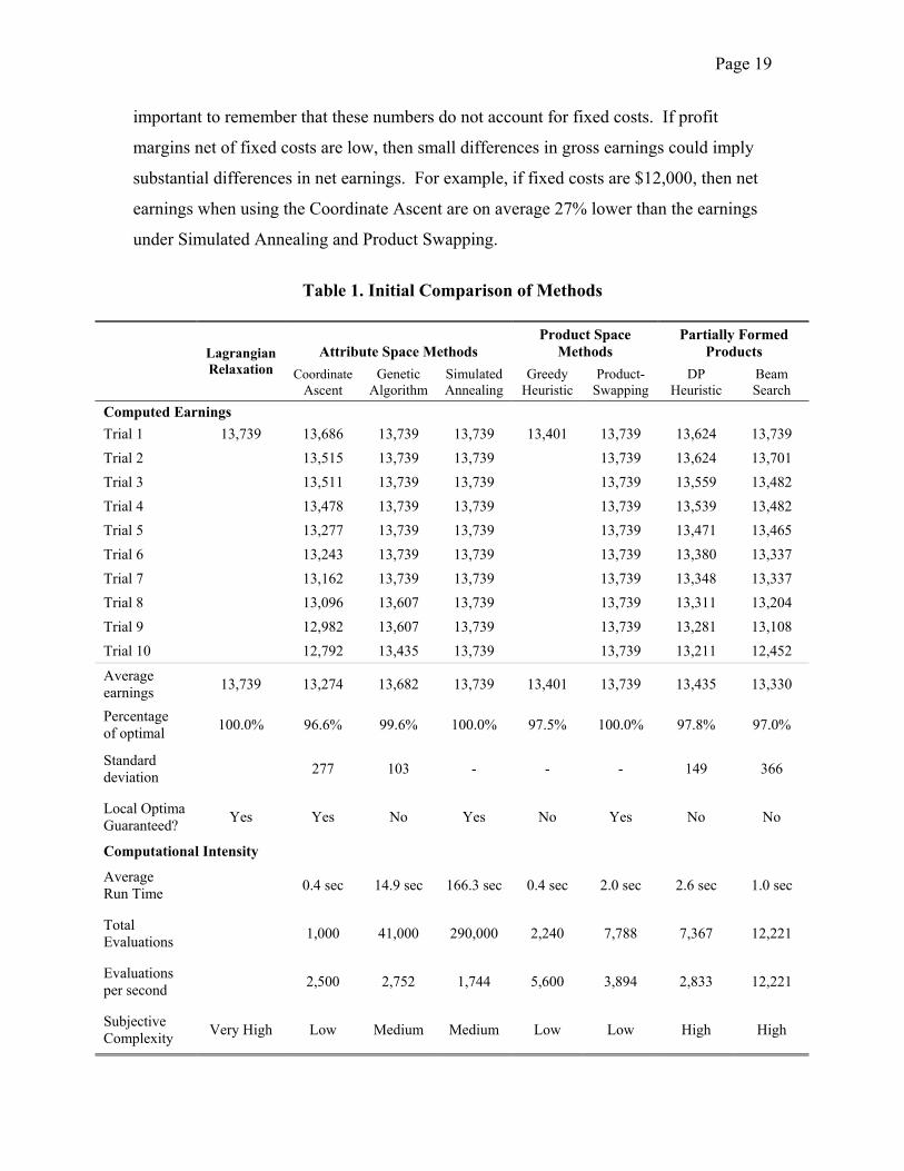
5. Tournament Results Table 1 presents results for ten trials of each optimization method, using the original set

of consumer part-worth data. In this initial analysis we assume that the part-worths are

measured without error and so interpret them as the “true” part-worths. We later

investigate what happens when we add errors to these part-worths. For each method, the

table reports measures describing the accuracy, computational intensity and the

complexity of the different methods.

Accuracy is measured by the earnings under each of the ten trials (presented in

descending order), together with the sample averages and standard deviations (where

appropriate) for each method. We also report whether each method guarantees that the

solution from each trial is locally optimal. In interpreting this guarantee, it is important

to recall that the definition of local optimum varies across the methods. For methods that

operate in attribute space, the “neighborhood” of locality is defined to include all

solutions that differ from the current solution by a single feature change in a single

product. In contrast, for methods that operate in product space, the local neighborhood is

defined to include all solutions that differ from the current solution by a single product,

which is a more rigorous standard of local optimality.

Computational intensity is measured by both the running time for one trial and the

number of product lines evaluated in each trial. Running time was measured using an

IBM Thinkpad laptop with a 1.7-GHz Pentium processor and 512 MB of RAM.

The complexity of the methods is difficult to objectively measure. We report our

subjective assessment of relative complexity. In general, the methods we label as having

a “medium” or “high” level of sophistication require some problem-specific fine-tuning

of parameter values, while those we label as “low” sophistication do not.

Accuracy

There are several findings of interest. First, the earnings level of $13,739 calculated

using Lagrangian relaxation is the global optimum earnings of the problem. This solution

turns out to be unique (there is only one combination of bags that will yield this solution).

Amongst the more practical methods, Simulated Annealing and Product Swapping

perform best, reaching the optimal solution in all ten trials. The Genetic Algorithm also

performed very well, finding the optimal solution in seven of the ten trials.

The Greedy Heuristic is the only method (other than Lagrangean Relaxation) for which

performance does not vary across the trials. Recall that this method begins by finding the

single most profitable product. Conditional on this choice, it then finds the next most

profitable product, and so on. Because each of these sub-tasks has a unique solution and

does not vary due to any stochastic element, the outcome of repeated trials also does not

vary. This unique outcome was $13,401, which was just $338 (2.5%) less than the

optimal outcome.

Recall that neither Beam Search nor the DP Heuristic are well-suited to the problem that

we are studying. Both methods were designed for problems in which it is not possible to

enumerate the combination of possible products. In this setting enumeration is possible:

the nine product features and price yield just 448 different combinations of bags.

Nonetheless, both of the methods performed well, generally reaching a solution that was

within 2-3% of the optimal design. The Beam Search did find the optimal solution in one

of the ten trials, but exhibited fairly high variance, with one trial yielding an outcome that

was almost $1,300 (9.4%) less than the optimal outcome.

Coordinate Ascent had the lowest average earnings and did not find the optimal outcome

in any of the ten trials. The average earnings for this method were just over 3% less than

the optimal solution. While the differences in average earnings might appear small, it is

important to remember that these numbers do not account for fixed costs. If profit

margins net of fixed costs are low, then small differences in gross earnings could imply

substantial differences in net earnings. For example, if fixed costs are $12,000, then net

earnings when using the Coordinate Ascent are on average 27% lower than the earnings

under Simulated Annealing and Product Swapping.

Table 1. Initial Comparison of Methods

Attribute Space Methods Product Space

Methods Partially Formed

Products Lagrangian Relaxation Coordinate

Ascent Genetic

Algorithm Simulated Annealing

Greedy Heuristic

Product-Swapping

DP Heuristic

Beam Search

Computed Earnings Trial 1 13,739 13,686 13,739 13,739 13,401 13,739 13,624 13,739 Trial 2 13,515 13,739 13,739 13,739 13,624 13,701 Trial 3 13,511 13,739 13,739 13,739 13,559 13,482 Trial 4 13,478 13,739 13,739 13,739 13,539 13,482 Trial 5 13,277 13,739 13,739 13,739 13,471 13,465 Trial 6 13,243 13,739 13,739 13,739 13,380 13,337 Trial 7 13,162 13,739 13,739 13,739 13,348 13,337 Trial 8 13,096 13,607 13,739 13,739 13,311 13,204 Trial 9 12,982 13,607 13,739 13,739 13,281 13,108 Trial 10 12,792 13,435 13,739 13,739 13,211 12,452

Average earnings 13,739 13,274 13,682 13,739 13,401 13,739 13,435 13,330

Percentage of optimal 100.0% 96.6% 99.6% 100.0% 97.5% 100.0% 97.8% 97.0%

Standard deviation 277 103 - - - 149 366

Local Optima Guaranteed? Yes Yes No Yes No Yes No No

Computational Intensity

Average Run Time 0.4 sec 14.9 sec 166.3 sec 0.4 sec 2.0 sec 2.6 sec 1.0 sec

Total Evaluations 1,000 41,000 290,000 2,240 7,788 7,367 12,221

Evaluations per second 2,500 2,752 1,744 5,600 3,894 2,833 12,221

Subjective Complexity Very High Low Medium Medium Low Low High High

There have been previous comparisons of selected pairs of these methods. Reassuringly,

the findings reported in Table 1 are consistent with these comparisons. For example,

Balakrishnan and Jacob (1996) present results comparing Genetic Algorithms and the DP

Heuristic. Their findings also favor the Genetic Algorithm. Similarly, Alexouda and

Paparizzos (2001) find that Genetic Algorithms outperform Beam Search, while Steiner

and Hruschka (2003) present evidence that Genetic Algorithms outperform the Greedy

Heuristic.

To help evaluate these findings, we also investigated two random strategies for choosing

bags. In the first random strategy we randomly chose five bags from the set of 448

possible bags. The average earnings level reached in one hundred random solutions was

only $8,071 (58.7% of the optimum). In the second random strategy we first chose three

bags to undercut the competitors and then randomly selected the other two bags. To

undercut the competitors we either matched the features and undercut the price, or

matched the price and added an additional feature. One hundred repetitions of this

strategy yielded average earnings of $9,458 (68.8% of the optimum).

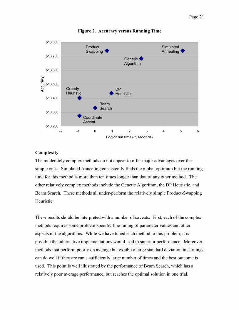
Computational Intensity

There is wide variation in the computational intensiveness of the methods, with running

times ranging from 0.4 seconds for the DP Heuristic to almost 3 minutes for Simulated

Annealing. In general, the more computationally intensive a method is, the better it

performs. We summarize this relationship in Figure 2, where we present a scatter plot of

the average accuracy (earnings) and the average running time. The outlier to this trend is

Product Swapping, which quickly achieves the maximum possible earnings using a

relatively small number of evaluations. In general, the methods that operate in product

space tend to outperform other methods with similar running times. The Product-

Swapping Heuristic outperforms Beam Search and the DP Heuristic, while the Greedy

Heuristic outperforms Coordinate Ascent.

Figure 2. Accuracy versus Running Time

$13,200

$13,300

$13,400

$13,500

$13,600

$13,700

$13,800

-2 -1 0 1 2 3 4 5 6

Log of run time (in seconds)

Acc

urac

ySimulated Annealing

Genetic Algorithm

Product Swapping

DP Heuristic

Beam Search

Coordinate Ascent

Greedy Heuristic

Complexity

The moderately complex methods do not appear to offer major advantages over the

simple ones. Simulated Annealing consistently finds the global optimum but the running

time for this method is more than ten times longer than that of any other method. The

other relatively complex methods include the Genetic Algorithm, the DP Heuristic, and

Beam Search. These methods all under-perform the relatively simple Product-Swapping

Heuristic.

These results should be interpreted with a number of caveats. First, each of the complex

methods requires some problem-specific fine-tuning of parameter values and other

aspects of the algorithms. While we have tuned each method to this problem, it is

possible that alternative implementations would lead to superior performance. Moreover,

methods that perform poorly on average but exhibit a large standard deviation in earnings

can do well if they are run a sufficiently large number of times and the best outcome is

used. This point is well illustrated by the performance of Beam Search, which has a

relatively poor average performance, but reaches the optimal solution in one trial.

Robustness Testing

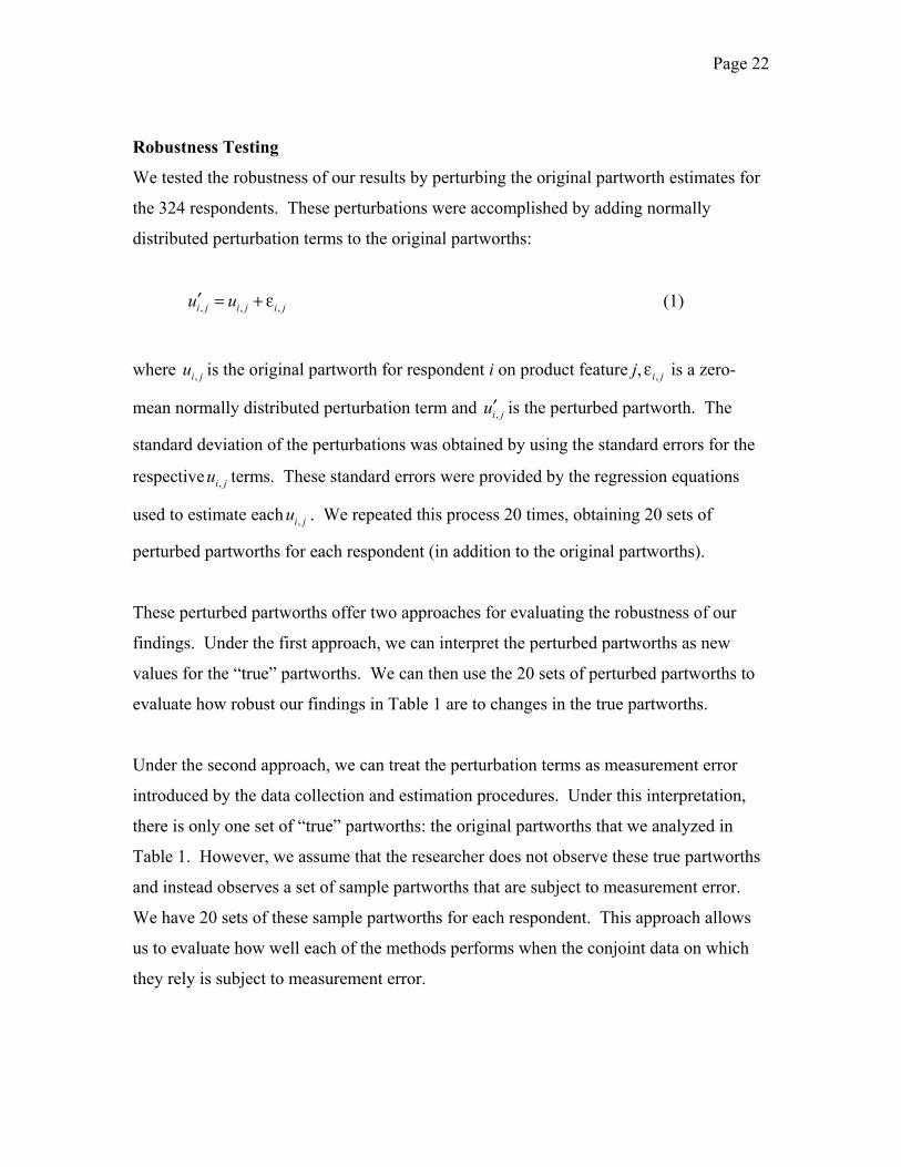
We tested the robustness of our results by perturbing the original partworth estimates for

the 324 respondents. These perturbations were accomplished by adding normally

distributed perturbation terms to the original partworths:

, ,i j i j i ju u′ = + ε , (1)

where u is the original partworth for respondent i on product feature j,ε is a zero-

mean normally distributed perturbation term and is the perturbed partworth. The

standard deviation of the perturbations was obtained by using the standard errors for the

respective terms. These standard errors were provided by the regression equations

used to estimate eachu . We repeated this process 20 times, obtaining 20 sets of

perturbed partworths for each respondent (in addition to the original partworths).

,i j ,i j

,i ju′

,i ju

,i j

These perturbed partworths offer two approaches for evaluating the robustness of our

findings. Under the first approach, we can interpret the perturbed partworths as new

values for the “true” partworths. We can then use the 20 sets of perturbed partworths to

evaluate how robust our findings in Table 1 are to changes in the true partworths.

Under the second approach, we can treat the perturbation terms as measurement error

introduced by the data collection and estimation procedures. Under this interpretation,

there is only one set of “true” partworths: the original partworths that we analyzed in

Table 1. However, we assume that the researcher does not observe these true partworths

and instead observes a set of sample partworths that are subject to measurement error.

We have 20 sets of these sample partworths for each respondent. This approach allows

us to evaluate how well each of the methods performs when the conjoint data on which

they rely is subject to measurement error.

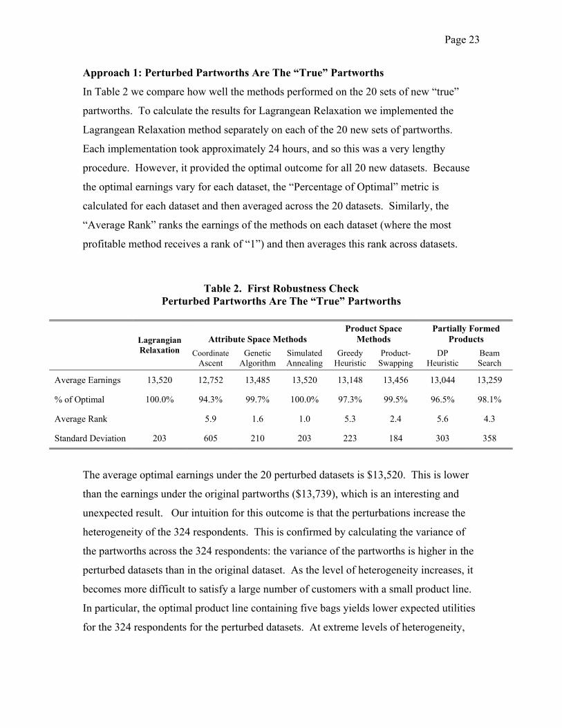
Approach 1: Perturbed Partworths Are The “True” Partworths

In Table 2 we compare how well the methods performed on the 20 sets of new “true”

partworths. To calculate the results for Lagrangean Relaxation we implemented the

Lagrangean Relaxation method separately on each of the 20 new sets of partworths.

Each implementation took approximately 24 hours, and so this was a very lengthy

procedure. However, it provided the optimal outcome for all 20 new datasets. Because

the optimal earnings vary for each dataset, the “Percentage of Optimal” metric is

calculated for each dataset and then averaged across the 20 datasets. Similarly, the

“Average Rank” ranks the earnings of the methods on each dataset (where the most

profitable method receives a rank of “1”) and then averages this rank across datasets.

Table 2. First Robustness Check Perturbed Partworths Are The “True” Partworths




Ascent Genetic


Greedy Heuristic

Product-Swapping

DP Heuristic

Beam Search

Average Earnings 13,520 12,752 13,485 13,520 13,148 13,456 13,044 13,259

% of Optimal 100.0% 94.3% 99.7% 100.0% 97.3% 99.5% 96.5% 98.1%

Average Rank 5.9 1.6 1.0 5.3 2.4 5.6 4.3

Standard Deviation 203 605 210 203 223 184 303 358

The average optimal earnings under the 20 perturbed datasets is $13,520. This is lower

than the earnings under the original partworths ($13,739), which is an interesting and

unexpected result. Our intuition for this outcome is that the perturbations increase the

heterogeneity of the 324 respondents. This is confirmed by calculating the variance of

the partworths across the 324 respondents: the variance of the partworths is higher in the

perturbed datasets than in the original dataset. As the level of heterogeneity increases, it

becomes more difficult to satisfy a large number of customers with a small product line.

In particular, the optimal product line containing five bags yields lower expected utilities

for the 324 respondents for the perturbed datasets. At extreme levels of heterogeneity,

each respondent would prefer a unique bag. At the other extreme, if all customers were

homogeneous, then they would all prefer the same bag.

Reassuringly, the other findings in Table 2 confirm the robustness of our earlier findings.

The methods that performed well on the original dataset (Table 1) also perform well on

the perturbed datasets. Simulated Annealing, Product Swapping and the Genetic

Algorithm have average earnings within 1% of the optimum, while the Greedy Heuristic,

Coordinate Ascent, the DP Heuristic, and Beam Search do less well.

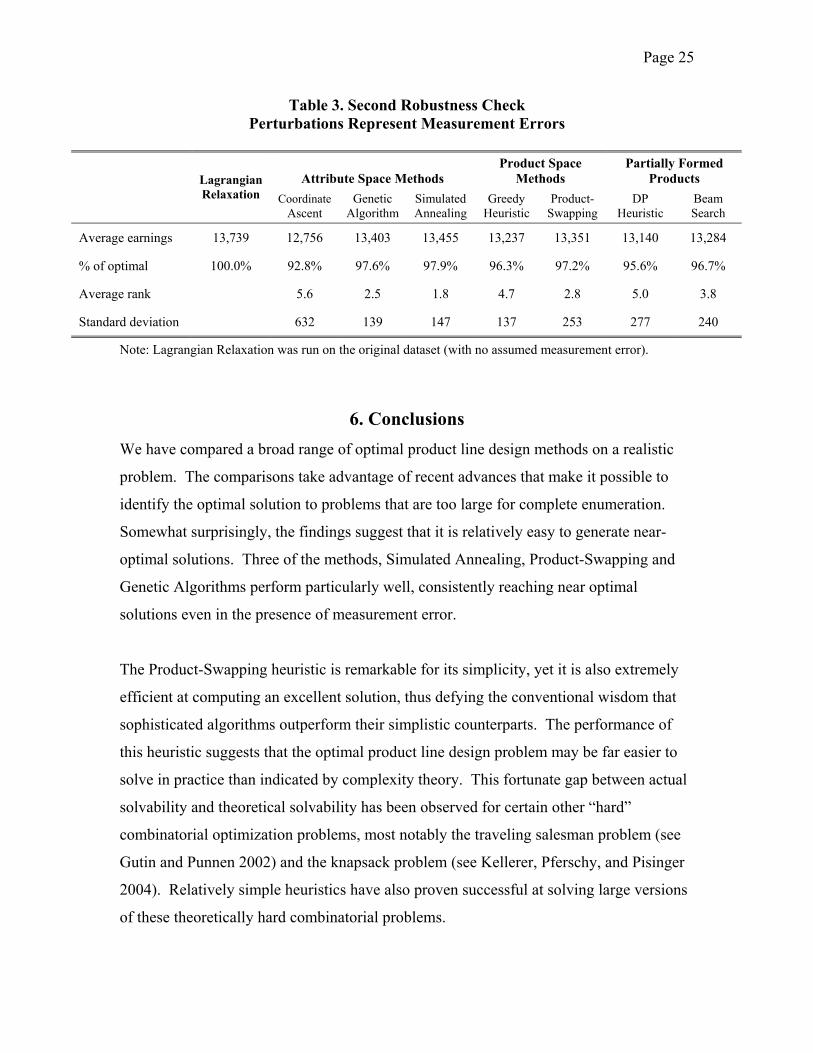
Approach 2: Perturbations Represent Measurement Error

In this second approach, we assume that the original data are consumers’ true partworths,

and that the 20 perturbed datasets represent measured partworths with measurement error

equal to the perturbations. The optimization methods are applied to the perturbed

datasets, and so they optimize over data containing measurement error. The “optimal”

product lines computed using the perturbed data are then evaluated on the original data

containing the “True” partworths. In this manner, we can compare the sensitivity of the

methods to measurement error.

Our findings are reported in Table 3. The “Average Earnings” and “Average Rank” are

calculated in a similar manner as in Table 2. However, in this case the earnings and rank

are evaluated using the original (unperturbed) data.

Once again, the methods that performed well on the original dataset (Table 1) also

perform well in this robustness check. Simulated Annealing, Product-Swapping and the

genetic Algorithm have average earnings within 3% of the true optimum. Most methods

now perform 2% to 4% worse than they do when we assume the dataset is 100%

accurate, reflecting the loss of information due to measurement error. Because

measurement errors affect most of the methods to a similar extent, there is little change in

the relative performance of the methods. Across the seven methods, the correlation

coefficient in the Average Earnings between Tables 2 and 3 is 0.97.

Table 3. Second Robustness Check Perturbations Represent Measurement Errors




Ascent Genetic


Greedy Heuristic

Product-Swapping

DP Heuristic

Beam Search

Average earnings 13,739 12,756 13,403 13,455 13,237 13,351 13,140 13,284

% of optimal 100.0% 92.8% 97.6% 97.9% 96.3% 97.2% 95.6% 96.7%

Average rank 5.6 2.5 1.8 4.7 2.8 5.0 3.8

Standard deviation 632 139 147 137 253 277 240

Note: Lagrangian Relaxation was run on the original dataset (with no assumed measurement error).

6. Conclusions We have compared a broad range of optimal product line design methods on a realistic

problem. The comparisons take advantage of recent advances that make it possible to

identify the optimal solution to problems that are too large for complete enumeration.

Somewhat surprisingly, the findings suggest that it is relatively easy to generate near-

optimal solutions. Three of the methods, Simulated Annealing, Product-Swapping and

Genetic Algorithms perform particularly well, consistently reaching near optimal

solutions even in the presence of measurement error.

The Product-Swapping heuristic is remarkable for its simplicity, yet it is also extremely

efficient at computing an excellent solution, thus defying the conventional wisdom that

sophisticated algorithms outperform their simplistic counterparts. The performance of

this heuristic suggests that the optimal product line design problem may be far easier to

solve in practice than indicated by complexity theory. This fortunate gap between actual

solvability and theoretical solvability has been observed for certain other “hard”

combinatorial optimization problems, most notably the traveling salesman problem (see

Gutin and Punnen 2002) and the knapsack problem (see Kellerer, Pferschy, and Pisinger

2004). Relatively simple heuristics have also proven successful at solving large versions

of these theoretically hard combinatorial problems.

We caution that the findings are subject to several potential limitations. The first

limitation is that our measure of accuracy presumes that the partworths accurately

describe actual customer behavior. Although we were able to demonstrate that the results

are robust to moderately large unbiased errors in the partworth estimates, they may not

survive systematic biases in these estimates. Of course this limitation relates not just to

optimization, but to conjoint analysis itself. If conjoint analysis provides inaccurate

predictions of market share, then little information is learned from the analysis. If these

biases can be predicted, it may be possible to develop a model that does describe actual

behavior. For example, Kivetz, Netzer, and Srinivasan (2003) find that modifying

conjoint analysis to incorporate a compromise effect significantly improves choice

predictions. Further research would then be required to investigate how such

modifications to the objective function affect the relative performance of the different

optimization methods.

A related issue is whether cost predictions are accurate enough to make optimal product

line design meaningful. Srinivasan, Lovejoy, and Beach (1997) find that for some

product types a simple linear cost model leaves much of the variance in product cost

unexplained. Again, if it were possible to develop a more realistic model of product cost,

the optimization methods could be modified to use the improved predictions. However,

it is not clear how well the optimization methods would perform on the modified

problem.

A third concern is that none of the optimization methodologies consider the competitive

response to new product introductions. The optimal solutions all predict large market

shares for the focal firm, which could reasonably be expected to provoke an aggressive

competitive reaction. Dobson and Kalish (1988) develop an optimization methodology

that accounts for price response by competitors, but at the cost of significantly increased

computation times. Developing an optimization methodology that adequately accounts

for competitive reaction and is tractable for large-scale design problems remains an

important challenge for future research.

Finally, while we have been able to evaluate a product line design problem that is

dramatically larger than those previously studied, the problem is still at the lower bound

of problems that firms would like to solve in practice. In time, as both the algorithms and

computational power improve, we anticipate that the frontier of problems that can be

evaluated will continue to extend.

References

Aarts, E., J. Korst, and P. van Laarhoven. “Simulated Annealing.” in Local Search in Combinatorial Optimization, E. Aarts and J.K. Lenstra (Eds.), John Wiley & Sons, Chichester, UK, 1997, 91-120.

Alexouda, G. and K. Paparrizos, “A Genetic Algorithm Approach To The Product Line Design Problem Using The Seller's Return Criterion: An Extensive Comparative Computational Study,” Euro. J. Oper. Res., 134, 1 (2001), 165-178.

Balakrishnan, P. V. and V. S. Jacob, “Genetic Algorithms For Product Design,” Management Sci., 42, 8 (1996), 1105-1117.

Belloni, Alexandre, N., “Lagrangian Relaxation for Computing Optimal Product Line Designs,” in preparation, MIT, Cambridge MA.

Bonnans, J. F., Gilbert, J. Ch., Lemaréchal, C., and Sagastizábal, C., Numerical Optimization: Theoretical and Practical Aspects, Universitext, Springer-Verlag, Berlin, 2003, xiv+423.

Dobson, G. and S. Kalish, “Positioning and Pricing A Product Line,” Marketing Sci., 7, 2 (1988), 107-125.

Dobson, G. and S. Kalish, “Heuristics For Pricing And Positioning A Product Line Using Conjoint And Cost Data,” Management Sci., 39, 2 (1993), 160-175.

Green, P. E. and A. M. Krieger, “Models And Heuristics For Product Line Selection,” Marketing Sci., 4, 1 (1985), 1-19

Green, P. E. and A. M. Krieger, “Conjoint Analysis With Product-Positioning Applications,” in Handbooks in OR & MS, Vol 5, J. Eliashberg and G. L. Lilien (Eds.), Elsevier Science B.V., City, state, 1993, 467-515.

Green, P. E., A. M. Krieger, and R. N. Zelnio, “A Componential Segmentation Model With Optimal Design Features,” Decision Sciences, 20, 2 (1989), 221-238.

Gutin G. and Punnen, A., The Traveling Salesman Problem and its Variation, Kluwer Academic Publishes, 2002.

Hauser, J. R., “Competitive Price and Positioning Strategies,” Marketing Sci., 7, 1 (1988), 76-91.

Hauser, J. R. and P. Simmie, “Profit Maximizing Perceptual Positions: An Integrated Theory for the Selection of Product Features and Price,” Management Sci., 27, 1 (1981), 33-56.

Huber, J. and J. A. Fiedler, “Comparing Perceptual Mapping and Conjoint Analysis: The Political Landscape,” 1996 Sawtooth Software Conference Proceedings.

Lucena, A., “Steiner Problem In Graphs: Lagrangean Relaxation And Cutting-Planes,” COAL Bulletin, 21:2-8, 1992.

Kellerer, H., Pferschy, U., and Pisinger, D., Knapsack Problems, Springer, 2004.

Kivetz, R., O. Netzer, and V. Srinivasan, “Alternative Models for Capturing the Compromise Effect,” J. Marketing Res., 41, 3 (2004), 237-257.

Kohli, R. and R. Krishnamurti, “A Heuristic Approach To Product Design,” Management Sci., 33, 12 (1987), 1523-1533.

Kohli, R. and R. Krishnamurti, “Optimal Product Design Using Conjoint Analysis: Computational Complexity And Algorithms,” Euro. J. Oper. Res., 40 (1989), 186-195.

Kohli, R. and R. Sukumar, “Heuristics For Product-Line Design Using Conjoint Analysis,” Management Sci., 36, 12 (1990), 1464-1478.

Martin, R. K., Large Scale Linear and Integer Optimization: A Unified Approach, Kluwer Academic Publishers, Dordrecht, The Netherlands, 1999.

McBride, R. D. and F. S. Zufryden, “An Integer Programming Approach to the Optimal Product Line Selection Problem,” Marketing Sci., 7, 2 (1988), 126-140.

Nair, S. K., L. S. Thakur, and K. Wen, “Near Optimal Solutions For Product Line Design And Selection: Beam Search Heuristics,” Management Sci., 41, 5 (1995), 767-785.

Nemhauser, G. L., Wolsey, L. A., and Fisher, M. L.,“An Analysis of Approximations for Maximizing Submodular Set Functions – I,” Mathematical Programming, 14:265-294, 1978.

Sawtooth Software, “Advanced Simulation Module (ASM) for Product Optimization,” Sawtooth Software Technical Paper Series, 2003.

Srinivasan, V., W. Lovejoy, and D. Beach, “Integrated Product Design for Marketability and Manufacturing,” J. Marketing Res., 34, 1 (1997), 154-163.

Steiner, W. and H. Hruschka, “Genetic Algorithms For Product Design: How Well Do They Really Work?” International Journal of Market Research, 45, 2 (2003), 229-240.

Toubia, O., D. I. Simester, J. R. Hauser, and E. Dahan, “Fast Polyhedral Adaptive Conjoint Estimation,” Marketing Sci., 22, 3 (2003), 273-303.

Zufryden, F., “A Conjoint Measurement-Based Approach for Optimal New Product Design and Market Segmentation,” in Analytical Approaches to Product and Marketing Planning, A. D. Shocker (ed.), Marketing Science Institute, Cambridge, MA, 1979.

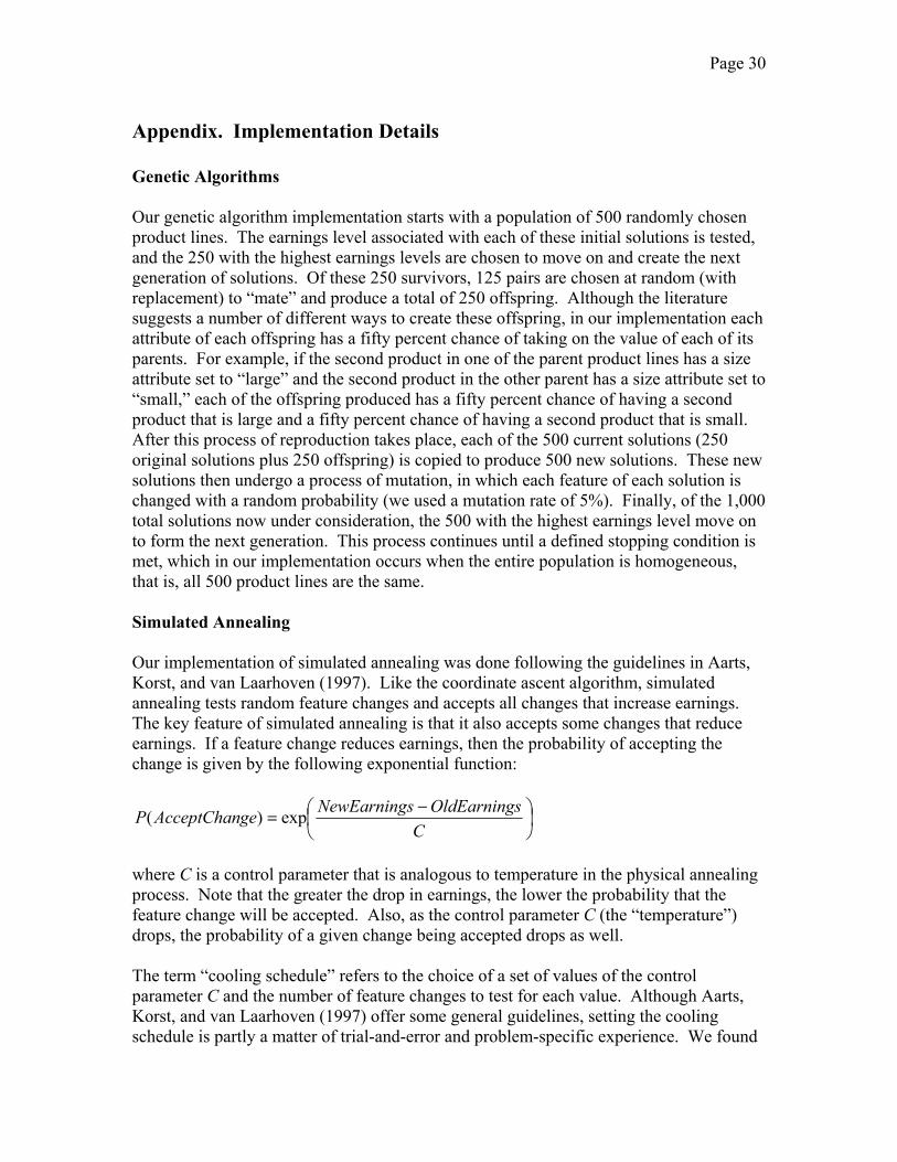
Appendix. Implementation Details Genetic Algorithms Our genetic algorithm implementation starts with a population of 500 randomly chosen product lines. The earnings level associated with each of these initial solutions is tested, and the 250 with the highest earnings levels are chosen to move on and create the next generation of solutions. Of these 250 survivors, 125 pairs are chosen at random (with replacement) to “mate” and produce a total of 250 offspring. Although the literature suggests a number of different ways to create these offspring, in our implementation each attribute of each offspring has a fifty percent chance of taking on the value of each of its parents. For example, if the second product in one of the parent product lines has a size attribute set to “large” and the second product in the other parent has a size attribute set to “small,” each of the offspring produced has a fifty percent chance of having a second product that is large and a fifty percent chance of having a second product that is small. After this process of reproduction takes place, each of the 500 current solutions (250 original solutions plus 250 offspring) is copied to produce 500 new solutions. These new solutions then undergo a process of mutation, in which each feature of each solution is changed with a random probability (we used a mutation rate of 5%). Finally, of the 1,000 total solutions now under consideration, the 500 with the highest earnings level move on to form the next generation. This process continues until a defined stopping condition is met, which in our implementation occurs when the entire population is homogeneous, that is, all 500 product lines are the same. Simulated Annealing Our implementation of simulated annealing was done following the guidelines in Aarts, Korst, and van Laarhoven (1997). Like the coordinate ascent algorithm, simulated annealing tests random feature changes and accepts all changes that increase earnings. The key feature of simulated annealing is that it also accepts some changes that reduce earnings. If a feature change reduces earnings, then the probability of accepting the change is given by the following exponential function:

−=

CsOldEarningsNewEarninggeAcceptChanP exp)(

where C is a control parameter that is analogous to temperature in the physical annealing process. Note that the greater the drop in earnings, the lower the probability that the feature change will be accepted. Also, as the control parameter C (the “temperature”) drops, the probability of a given change being accepted drops as well. The term “cooling schedule” refers to the choice of a set of values of the control parameter C and the number of feature changes to test for each value. Although Aarts, Korst, and van Laarhoven (1997) offer some general guidelines, setting the cooling schedule is partly a matter of trial-and-error and problem-specific experience. We found

that it was best to start with a value large enough that almost all feature changes are accepted, calculate each subsequent value by multiplying the current value by 0.8, and end with a value small enough that very few negative changes are accepted. We divided the problem into 29 time stages, and tested 10,000 feature changes in each stage, yielding a total of 290,000 tested feature changes. The control parameter was set at each stage according to the following schedule: 1443, 1154, 923, 739, 591, 473, 378, 303, 242, 194, 155, 124, 99, 79, 63, 51, 41, 32, 26, 21, 17, 13, 11, 9, 7, 5, 4, 3, 0.1.

Optimizing Product Line Designs: Efficient Methods and ...

Documents

Transcript of Optimizing Product Line Designs: Efficient Methods and ...