Optimizing Katsevich Image Reconstruction Algorithm on Multicore

Processors

Eric Fontaine GeorgiaTech

Hsien-Hsin Lee GeorgiaTech

2

Outline

• Image Reconstruction Overview• Katsevich Algorithm• Prior Work and Our Optimizations:

– PI-Interval Method– Cone-Beam Cover Method

• Our Work:– Symmetry Method

• Results• Conclusion

3

Image Reconstruction Overview

• Is it possible to reconstruct the 3-D volume of an object from projections?– Early 20th century: Radon Transform and Fourier Slice Theorem

• Common methods– MRI

• Noninvasive magnetic field applied.• Main function FFT.

– Positron Emission Tomography• Patient injected with radioactive matter.• When decay, release radiation which is detected by sensors.

– Computed Tomography• Use x-ray projections of object.• Use filtered back-projection to obtain original volume.

• Contain fine-grained and coarse-grained data parallelism.

4

Fourier Slice Theorem

• Fourier Transform of 1-D Projection of 2-D Image = Slice of 2-D Fourier Transform of Image

• Formula can be rearranged as filtered backprojection.

5

Filtered-Backprojection

• After projections filtered, then backprojected.– Less computationally expensive than filtering after backprojection.

• Require 180 degrees of projection data.• Can be extended to fan-beams instead of parallel-beams.

Projection Backprojection

6

3-D Volume?

• Previous methods for 2-D slices.• Can repeat for multiple slices to get 3-D volume.• Two common 3-D back-projection algorithms.

– FDK (1985)• Approximation, fast reconstruction.• Use projections taken on a circular path surrounding the

object.• More accurate on the plane containing the circle.• Can be generalized for helical scanning paths.

– Katsevich (2003)• Theoretically exact, but also more compute-intensive.• Use projections taken on a helical path surrounding the object.• Can reconstruct long objects, unlike the original FDK.• Fast scanning.

7

Katsevich Image Reconstruction

• Reconstruct density of 3-D cylindrical volume.– Analyze many 2-D cone-beam

projections taken along helical scanning path.

• First exact helical cone beam image reconstruction algorithm.

• Filtered-backprojection form.– More computationally

expensive than other non-exact algorithms such as FDK.

– Also requires differentiation and remapping of projections to and from filtering coordinates.

8

Katsevich Step 1: Differentiation

• Take difference between neighboring texels.• Take difference between neighboring projections.

Projection k

Projection k+1

Differentiated Projection k

9

Katsevich Step 2: Filtering

• Remap projection to filtering coordinates.• Perform horizontal convolution along kappa lines.• Remap back to projection coordinates.

10

Katsevich Step 3: Backprojection

• Backprojection

ProjectionBackprojection

X-ray projection source

Volume of Interest

Projection

• Projection is formed by line integral of density along path of ray from x-ray source to detector.

• Backprojection is the reverse – smear projection data from detector onto image voxel.

• Use linear interpolation of 4 neighboring texels when looking up backprojection value.

11

PI-Interval Method

• PI-Interval formed by line intersecting:– A point inside helix and two points on the helix

voxelPI-Interval

Helical Scanning Path

12

PI-Interval Method

• PI-Interval contains all data necessary for exact reconstruction.

• Iterate over all projections in PI-Interval containing each voxel.– Calculate voxel’s backprojected coordinate.– Get projection’s value at backprojected

coordinate using linear interpolation and weight appropriately.

– Accumulate contribution from each projection.– Use special weighting for beggining and end of

interval.

13

PI-Interval Method

Voxel Reconstruction Done!

14

PI-Interval Method

• Parallelization Strategy:

Proj 1

Proj2

Proj 3

Proj K

Diff Remap Convolve Remap

Diff Remap Convolve Remap Slice Z Max

Slice 1

• Assign projections to different threads.• Perform differentiation of each projection.• Remap projection to filtering coordinates.• Perform convolution along kappa lines.• Remap back to projection coordinates.• Barrier, then assign different image slices to different threads.• Each thread performs backprojection of its assigned slice.• Continue until all slices are done.

15

PI-Interval Method Basic Optimizations• Majority of time spent calculating PI-intervals and

backprojection.– PI-intervals are constant for a particular helix.

• Precompute one slice of PI-intervals.• PI-intervals for different horizontal slices can be determined by

rotation.• Easy ~25% speedup

• Next focused on backprojection inner loop.– Removed trival lookup tables.

• ~10% speedup.– Used sin, cos lookup tables.

• ~15% speedup.– Moved if statements for smoothing the ends of the PI-interval

outside loop.• Duplicated inner loop code.• ~10% speedup.

– Removed if statements for bounds testing the backprojected coordinates.

• Needed to add extra row and column slack to projection data.• ~3% speedup.

16

Cone-beam Cover Method• Formed by intersection of cone beam and volume.• Contain necessary data for reconstruction.

X-ray projection source

17

Cone-beam Cover Method• Access projection and image memory linearly.

– Rotate projection 90 degrees.• Accumulate partial image reconstruction.• Iterate from bottom to top of projection.• Bring in two columns of projection data.

18

Cone-beam Cover Method

• Parallelization Strategy:

Proj 1

Proj2

Proj 3

Proj K

Diff Remap Convolve Remap

Diff Remap Convolve Remap

Shared

Image

Memory

• Assign projections to different threads.• Perform differentiation of each projection.• Remap projection to filtering coordinates.• Perform convolution along kappa lines.• Remap back to projection coordinates.• Each thread performs backprojection of its assigned projection to shared image memory.

• Continue until all projections are done.

19

SIMD Optimizations

• Use SIMD for backprojection.– Backproject 4 consecutive z voxels at a time.– Requires data shuffling.– Not all memory access are aligned.– Treat top and bottom of cone beam cover

specially.

• Use SIMD for differentiation and remapping steps.– Act on 4 consecutive texels at a time

20

Symmetry Method

• Exploit backprojection redundancy among every π/2 source projection– due to π/2 symmetry of sin, cos.

•Reduce backprojection calculations by ~4x for

each turn of helix

21

Symmetry Method

• Unpacked Image Data • Packed Image Data

Z Offset 0Z Offset 1

• All the colored voxels have identical backprojection coordinates

• Pack them so they occupy adjacent memory locations

• Voxels with same relative “z offset” grouped together

22

Symmetry Method

• Easily SIMDified.– No need for projection or image data shuffling.– All 128-bit memory access are aligned.– Need projection packing step (outside of main

loop).– Need image unpacking step (outside of main

loop).– Inner loop primarily consists of SIMD memory

accesses.• Coordinate and interpolation calculations outside of

inner loop.

23

Results

• System:– Two Intel 2.33 Ghz Quad Core Clovertown

processors.– 4 GB Ram.– Windows Vista.

• Programming:– C ported from open source Matlab implementation.– OpenMP.– Intel Performance Primitives.– Intrinsic Assembly.

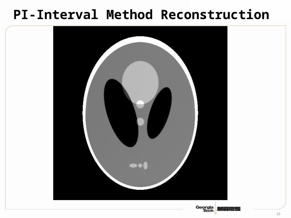
• Input: 2-D Projections of Shepp-Logan Phantom.– 4 helical turns plus 1 overscan turn.

• Output: 3-D density.

24

Original Shepp-Logan Phantom

25

PI-Interval Method Reconstruction

26

PI-Interval Method Error

27

Cone-beam Cover Method Reconstruction

28

Cone-beam Cover Method Error

29

Symmetry Method Reconstruction

30

Symmetry Method Error

31

Reconstruction Time

1283 image from 640 128x32 projections 2563 image from 1280 256x64 projections

5123 image from 2560 512x128 projections 10243 image from 5120 512x128 projections

32

Comparison to U Iowa

1283 image from 640 128x32 projections 2563 image from 1280 256x64 projections

• ~ 73x speedup for Symmetry Method over U Iowa for 256^3 running on same system for 1 thread.

• Note: U Iowa implementation uses MPI.– Focused primarily on parallel speedup.

0

10

20

3040

50

60

70

1 2 3 4 5 6 7 8

Number of Threads

Exe

c T

ime

(Sec

)

U Iowa PI-interval method

Cone beam cover Symmetry

0

200

400

600

800

1000

1 2 3 4 5 6 7 8

Number of Threads

U Iowa PI-interval method

Cone beam cover Symmetry

33

Reconstruction Time Breakdown

Step Init-base Pi-

Method

Opt-1T Opt-2T Opt-4T Opt-8T

Derivative 20.6 3.8

25.0 (3.0x)

18.9 (4.0x)

18.8 (4.0x)

Forward remap

4.2 2.1

Convolve 18.9 19.5

Backward remap

31.8 2.5

SIMD Pack 0 12.5

Backproject

23722.2 (1.0x)

2083.9 (11.4x)

1062.0 (22.3x)

728.8 (32.5x)

623.5 (38.0x)

Total 23798.1 (1.0x)

2126.7 (11.2x)

1087.3 (21.9x)

748.2 (31.8x)

642.3 (37.1x)

Time in seconds (speedup) for 10243 image.

34

Scalability of Symmetry Method

35

Conclusion

• Majority of time spent in backprojection.• 37.1x speedup.

– Comparing final Symmetry Method running on eight threads to the baseline π-Interval Method running on a single thread for 1024 image reconstruction.

• Symmetry Method has poor multi-thread speedup because it is memory bound.

• Front-side bus bandwidth becomes saturated and limits scalability.

36

Questions?

37

Bus Utilization

0

10

20

30

40

50

60

70

80

90

100

1 2 3 4 5 6 7 8

Number of Threads

Bu

s U

tiliz

ati

on

% f

rom

Da

ta

(# bus cycles data ready line high / number bus cycles) average for inner loop

1024^3 reconstruction for 60 seconds after 60 seconds warmup

38

Difference between PI-Method & Cone-Beam

39

Difference between PI-Method & Symmetry

40

Difference between Cone-Beam & Symmetry

41

Symmetry Method: Projection Packing

•Interleave columns of projections•Linear access to projection memory.