Optimizing Grouped Aggregation inGeo-Distributed Streaming Analytics

Benjamin HeintzUniversity of Minnesota

Minneapolis, MNheintz@cs.umn.edu

Abhishek ChandraUniversity of Minnesota

Minneapolis, MNchandra@cs.umn.edu

Ramesh K. SitaramanUMass, Amherst & Akamai

Tech. Amherst, MAramesh@cs.umass.edu

ABSTRACTLarge quantities of data are generated continuously overtime and from disparate sources such as users, devices, andsensors located around the globe. This results in the needfor efficient geo-distributed streaming analytics to extracttimely information. A typical analytics service in these set-tings uses a simple hub-and-spoke model, comprising a sin-gle central data warehouse and multiple edges connectedby a wide-area network (WAN). A key decision for a geo-distributed streaming service is how much of the computa-tion should be performed at the edge versus the center. Inthis paper, we examine this question in the context of win-dowed grouped aggregation, an important and widely usedprimitive in streaming queries. Our work is focused on de-signing aggregation algorithms to optimize two key metricsof any geo-distributed streaming analytics service: WANtraffic and staleness (the delay in getting the result). To-wards this end, we present a family of optimal offline al-gorithms that jointly minimize both staleness and traffic.Using this as a foundation, we develop practical online ag-gregation algorithms based on the observation that groupedaggregation can be modeled as a caching problem wherethe cache size varies over time. This key insight allows usto exploit well known caching techniques in our design ofonline aggregation algorithms. We demonstrate the prac-ticality of these algorithms through an implementation inApache Storm, deployed on the PlanetLab testbed. The re-sults of our experiments, driven by workloads derived fromanonymized traces of a popular web analytics service offeredby a large commercial CDN, show that our online aggrega-tion algorithms perform close to the optimal algorithms fora variety of system configurations, stream arrival rates, andquery types.

Categories and Subject DescriptorsC.2.4 [Distributed Systems]: Distributed Applications

Permission to make digital or hard copies of all or part of this work for personal orclassroom use is granted without fee provided that copies are not made or distributedfor profit or commercial advantage and that copies bear this notice and the full cita-tion on the first page. Copyrights for components of this work owned by others thanACM must be honored. Abstracting with credit is permitted. To copy otherwise, or re-publish, to post on servers or to redistribute to lists, requires prior specific permissionand/or a fee. Request permissions from permissions@acm.org.HPDC’15, June 15–20, 2015, Portland, Oregon, USA.Copyright c© 2015 ACM 978-1-4503-3550-8/15/06 . . . $15.00.http://dx.doi.org/10.1145/2749246.2749276.

KeywordsGeo-distributed systems, stream processing, aggregation, Storm

1. INTRODUCTIONData analytics is undergoing a revolution: both the vol-

ume and velocity of analytics data are increasing at a rapidrate. Across a large number of application domains thatinclude web analytics, social analytics, scientific computing,and energy analytics, large quantities of data are generatedcontinuously over time in the form of posts, tweets, logs, sen-sor readings, etc. A modern analytics service must providereal-time analysis of these data streams to extract meaning-ful and timely information for the user. As a result, there hasbeen a growing interest in streaming analytics with recentdevelopment of several distributed analytics platforms [2, 8,28].

In many streaming analytics domains, data is often de-rived from disparate sources that include users, devices, andsensors located around the globe. As a result, the dis-tributed infrastructure of a typical analytics service (e.g.,Google Analytics, Akamai Media Analytics, etc.) has a hub-and-spoke model (see Figure 1). The data sources generateand send a stream of data to “edge” servers near them. Theedge servers are geographically distributed and process theincoming data and send it to a central location that canprocess the data further, store the summaries, and presentthose summaries in visual form to the user of the analyticsservice. While the central location that acts as a hub is of-ten located in a well-provisioned data center, the resourcesare typically limited at the edge locations. In particular, theavailable WAN bandwidth between the edge and the centermight be limited.

A traditional approach to analytics processing is the cen-tralized model where no processing is performed at the edgesand all the data is sent to a dedicated centralized location.However, such an approach is often inadequate or subopti-mal, since it can strain the scarce WAN bandwidth availablebetween the edge and the center, cause longer delays due tothe high volumes of unaggregated data to be sent over thenetwork, and does not make use of the available computeand storage resources at the edge. An alternative is a decen-tralized approach [23] that utilizes the edge for much of theprocessing in order to minimize the amount of WAN traf-fic. In this paper, we argue that analytics processing mustutilize both edge and central resources in a carefully coordi-nated manner in order to achieve the stringent requirementsof an analytics service in terms of both network traffic anduser-perceived delay.

Wide-Area Network

Edge Server

Central Data Warehouse

Edge Server

Edge Server

Figure 1: The distributed model for a typical ana-lytics service comprises a single center and multipleedges, connected by a wide-area network.

An important primitive in any analytics system is groupedaggregation. Grouped aggregation is used to combine andsummarize large quantities of data from one or more datastreams. As a result, it is provided as a key operator in mostdata analytics frameworks, such as the Reduce operation inMapReduce, or GroupBy in SQL and LINQ. A commonvariant of the primitive in stream computing is windowedgrouped aggregation where data produced within finite speci-fied time windows must be summarized. Windowed groupedaggregation is one of the most frequently used primitivesin an analytics service and underlies queries that aggregatea metric of interest over a time window. For instance, aweb analytics user may wish to compute the total visits tohis/her web site broken down by country and aggregatedon an hourly basis to gauge the current content popularity.Similarly, a network operator may want to compute the av-erage load in different parts of the network every 5 minutesto identify hotspots. In these cases, the user would define astanding windowed grouped aggregation query that gener-ates results periodically for each time window (every hour,5 minutes, etc.).

Our work is focused on designing algorithms for perform-ing windowed grouped aggregation in order to optimize thetwo key metrics of any geo-distributed streaming analyticsservice: WAN traffic and staleness (the delay in getting theresult for a time window). A service provider typically paysfor the WAN bandwidth used by its deployed servers [3,13]. In fact, bandwidth cost incurred due to WAN traffic isa significant component of the operating expense (OPEX)of the service provider infrastructure, the other key compo-nents being colocation and power costs. Therefore reducingWAN traffic represents an important cost-saving opportu-nity. In addition, reducing staleness is critical in order todeliver timely results to applications and is often a part ofthe SLA for analytics services. While much of the existingwork on decentralized analytics [23, 25] has focused primar-ily on optimizing a single metric (e.g., network traffic), itis important to examine both traffic and staleness togetherto achieve both cost savings as well as higher informationquality.

The key decision that our algorithms make is how muchof the data aggregation should be performed at the edge ver-sus the center. To understand the challenge, consider twoalternate approaches to grouped aggregation: pure stream-ing, where all data is immediately sent from the edge tothe center without any edge processing; and pure batching,where all data during a time window is aggregated at the

edge, with only the aggregated results being sent to the cen-ter at the end of the window. Pure batching results in agreater level of edge aggregation, resulting in a reduction inthe edge-to-center WAN traffic compared to pure streaming.However, the edge must wait longer to collect more data foraggregation, risking the possibility of the aggregates reach-ing the center late, resulting in greater staleness. We haveshown [15] that the decision about how much aggregation tobe performed at the edge cannot be made statically; rather itdepends on several factors such as the query type, networkconstraints, data arrival rates, etc. Further, these factorsvary significantly over time (see Figure 2(b)), requiring thedesign of algorithms that can adapt to changing factors in adynamic fashion.

Research Contributions• To our knowledge, we provide the first algorithms andanalysis for optimizing grouped aggregation, a key primitive,in a wide-area streaming analytics service. In particular,we show that simpler approaches such as pure streaming orbatching do not jointly optimize traffic and staleness, andare hence suboptimal.• We present a family of optimal offline algorithms thatjointly minimize both staleness and traffic. Using this asa foundation, we develop practical online aggregation algo-rithms that emulate the offline optimal algorithms.• We observe that grouped aggregation can be modeled asa caching problem where the cache size varies over time.This key insight allows us to exploit well known cachingalgorithms in our design of online aggregation algorithms.•We demonstrate the practicality of these algorithms throughan implementation in Apache Storm [2], deployed on thePlanetLab [1] testbed. Our experiments are driven by work-loads derived from traces of a popular web analytics serviceoffered by Akamai [19], a large content delivery network.The results of our experiments show that our online aggre-gation algorithms simultaneously achieve traffic within 2.0%of optimal while reducing staleness by 65% relative to batch-ing. We also show that our algorithms are robust to a varietyof system configurations (number of edges), stream arrivalrates, and query types.

2. PROBLEM FORMULATION

System Model.We consider the typical hub-and-spoke architecture of an

analytics system with a center and multiple edges (see Fig-ure 1). Data streams are first sent from each source to aproximal edge. The edges collect and (potentially, partially)aggregate the data. The aggregated data can then be sentfrom the edges to the center where more aggregation couldhappen. The final aggregated results are available at thecenter. Users of the analytics service query the center to vi-sualize the data. To perform grouped aggregation, each edgeruns a local aggregation algorithm: it acts independently todecide when and how much to aggregate the incoming data.

Data Streams and Grouped Aggregation.A data stream comprises records of the form (k, v) where

k is the key and v is the value of the record. Data recordsof a stream arrive at the edge over time. Each key k canbe multi-dimensional, with each dimension corresponding to

a data attribute. A group is a set of records that have thesame key.

Windowed grouped aggregation over a time window [t, t+W ), where W is the user-specified window size, is defined asfollows from an input/output perspective. The input is theset of data records that arrive within the time window. Theoutput is determined by first placing the data records intogroups where each group is a set of records with the samekey. For each group {(k, vi)}, 1 ≤ i ≤ n, that correspondto the n records in the time window that have key k, anaggregate value v = v1⊕ v2 · · ·⊕ vn is computed, where ⊕ isany associative binary operator1. Examples of aggregates in-clude sums, histograms, and approximate data types such asBloom filters. Customarily, the timeline is subdivided intonon-overlapping intervals of size W and windowed group ag-gregation is computed on each such window2. Note that theaggregate record is typically of the same size as an incomingdata record. Thus, grouped aggregation results in a reduc-tion in the amount of data.

To compute windowed grouped aggregation, we consideraggregation at the edge as well as the center. The datarecords that arrive at the edge can be partially aggregatedlocally at the edge, so that the edge can maintain a set ofpartial aggregates, one for each distinct key k. The edge maytransmit, or flush these aggregates to the center; we refer tothese flushed records as updates. The center can furtherapply the aggregation operator ⊕ on incoming updates asneeded in order to generate the final aggregate result. Weassume that the computational overhead of the aggregationoperator ⊕ is a small constant compared to the networkoverhead of transmitting an update.

Optimization Metrics.Our goal is to simultaneously minimize two metrics: stal-

eness, a key measure of information quality; and networktraffic, a key measure of cost. Staleness is defined as thesmallest time s such that the results of grouped aggrega-tion for time window [t, t+W ) are available at the center attime t + W + s. In our model, staleness is simply the timeelapsed from when the time window completes to when thelast update for that time window reaches the center and isincluded in the final aggregate. Roughly, staleness is the de-lay measured from when all the data has arrived to when ananalytics user views the results of her grouped aggregationquery. The network traffic is measured by the number ofupdates sent over the network from the edge to the center.

Algorithms for Grouped Aggregation.An aggregation algorithm runs on the edge and takes as

input the sequence of arrivals for data records in a giventime window [t, t + W ). The algorithm produces as outputa sequence of updates that are sent to the center. For eachdistinct key k with nk arrivals in the time window, supposethat the ith data record (k, vi,k) arrives at time ai,k, wheret ≤ ai,k < t+W and 1 ≤ i ≤ nk. For each key k, the outputof the aggregation algorithm is a sequence of mk updateswhere the ith update (k, vi,k) departs for the center at time

1More formally, any binary operator that forms a semigroupcan be used.2Such non-overlapping time windows are often called tum-bling windows in analytics terminology.

di,k, 1 ≤ i ≤ mk. The updates must have the followingproperties:• Each update for each key k aggregates all values for thatkey in the current time window that have not been previ-ously aggregated.• Each key k that has nk > 0 arrivals must have mk > 0updates such that dmk,k ≥ ank,k. That is, each key withan arrival must have at least one update and the last up-date must depart after the final arrival so that all the valuesreceived for the key have been aggregated.

The goal of the aggregation algorithm is to minimize traf-fic which is simply the total number of updates, i.e.,

∑kmk.

The other simultaneous goal is to minimize staleness whichis the time for the final update to reach the center, i.e., theupdate with the largest value for dmk,k, to reach the center3.

3. DATASET AND WORKLOADTo derive a realistic workload for evaluating our aggrega-

tion algorithms, we have used anonymized workload tracesobtained from a real-life analytics service4 offered by Akamaiwhich operates a large content delivery network. The down-load analytics service is used by content providers to trackimportant metrics about who is downloading their content,from where is it being downloaded, what was the perfor-mance experienced by the users, how many downloads com-pleted, etc. The data source is a software called downloadmanager that is installed on mobile devices, laptops, anddesktops of millions of users around the world. The down-load manager is used to download software updates, securitypatches, music, games, and other content. The downloadmanagers installed on users’ devices around the world sendinformation about the downloads to the widely-deployededge servers using “beacons”5. Each download results inone or more beacons being sent to an edge server containinginformation pertaining to that download. The beacons con-tain anonymized information about the time the downloadwas initiated, url, content size, number of bytes downloaded,user’s ip, user’s network, user’s geography, server’s networkand server’s geography. Throughout this paper, we use theanonymized beacon logs from Akamai’s download analyticsservice for the month of December, 2010. Note that we nor-malize derived values from the data set such as data sizes,traffic sizes, and time durations, for confidentiality reasons.

Throughout our evaluation, we compute grouped aggre-gation for three commonly-used queries in the download an-alytics service. Queries that are issued in the download an-alytics service that use the grouped aggregation primitivecan be roughly classified according to query size that is de-fined to be the number of distinct keys that are possible forthat query. We choose three representative queries for dif-ferent size categories (see Table 1). The small query groupsby two dimensions with the key consisting of the tuple ofcontent provider id and the user’s last mile bandwidth clas-sified into four buckets. The medium query groups by threedimensions with the key consisting of the triple of the con-tent provider id, user’s last mile bandwidth, and the user’s

3We implicitly assume a FIFO ordering of data records overthe network, as is typically the case with protocols like TCP.4http://www.akamai.com/dl/feature_sheets/Akamai_Download_Analytics.pdf5A beacon is simply an http GET issued by the downloadmanager for a small GIF containing the reported values inits url query string.

Table 1: Queries used throughout the paper.Name Key Value (aggregate type) Description Query SizeSmall (cpid, bw) bytes downloaded (integer sum) Total bytes downloaded by content

provider by last-mile bandwidth.O(102) keys

Medium (cpid, bw, country_code) bytes downloaded (first 5 mo-ments)

Mean and standard deviation of to-tal bytes per download by contentprovider by bandwidth by country.

O(104) keys

Large (cpid, bw, url) client ip (HyperLogLog) Approximate number of uniqueclients by content provider by bwby url.

O(106) keys

100 101 102 103 104 105 106

Key Frequency

0.10.20.30.40.50.60.70.80.91.0

CD

F

largemediumsmall

(a) CDF of the frequency per key at a single edgefor the three queries.

0 1 2 3 4 5Time (day)

0.0

0.2

0.4

0.6

0.8

1.0

1.2

Nor

mal

ized

Uni

que

Key

s/h

r large medium small

(b) The unique key arrival rate for three differ-ent queries in a real-world web analytics service,normalized to the maximum rate for the largequery.

Figure 2: Akamai Web download service data set characteristics.

country code. The large query groups by a different setof three dimensions with the key consisting of the triple ofthe content provider id, the user’s country code, and the urlaccessed. Note that the last dimension—url—can take onhundreds of thousands of distinct values, resulting in a verylarge query size.

The total arrival rate of data records across all keys forall three queries is the same, since each arriving beacon con-tributes a data record for each query. However, the threequeries have a different distribution of those arrivals acrossthe possible keys as shown in Figure 2(a). Recall that thelarge query has a large number of possible keys. About 56%of the keys for the large query arrived only once in the tracewhereas the same percentage of keys for the medium andsmall query is 29% and 15% respectively. The median ar-rival rate per key was four (resp., nine) times larger for themedium (resp., small) query in comparison with the largequery. Figure 2(b) shows the number of unique keys arriv-ing per hour at an edge server for the three queries. Thefigure shows the hourly and daily variations and also thevariation across the three queries.

4. MINIMIZING WAN TRAFFIC AND STAL-ENESS

We now explore how to simultaneously minimize both traf-fic and staleness. We show that if the entire sequence ofupdates is known beforehand, then it is indeed possible tosimultaneously achieve the optimal value for both traffic andstaleness. While this offline solution is not implementable,it serves as a baseline to which any online algorithm canbe compared. Further, it characterizes the optimal solutionthat helps us evolve the more sophisticated online algorithmsthat we present in Section 5. Due to space constraints, we

omit the proofs of lemmas and theorems here; more detailscan be found in our technical report [14].

Lemma 1 (Traffic optimality). In each time win-dow, an algorithm is traffic-optimal iff it flushes exactly oneupdate to the center for each distinct key that arrived in thewindow.

Intuitively, this lemma states that multiple records foreach key within a window can be aggregated and sent as asingle update to minimize traffic. Note that a pure batchingalgorithm satisfies the above lemma, and hence is traffic-optimal, but may not be staleness-optimal.

We now present optimal offline algorithms that minimizeboth traffic and staleness, provided the entire sequence of keyupdates is known to our aggregation algorithm beforehand.

Theorem 2 (Eager Optimal Algorithm). There ex-ists an optimal offline algorithm that schedules its flusheseagerly; i.e., it flushes exactly one update for each distinctkey immediately after the last arrival for that key within thetime window.

Intuitively, this algorithm is traffic-optimal since it sendsonly one update per key, and is also staleness-optimal since itsends each update without any additional delay. We call theoptimal offline algorithm described above the eager optimalalgorithm due to the fact that it eagerly flushes updates foreach distinct key immediately after the final arrival to thatkey. This eager algorithm is just one possible algorithm toachieve both minimum traffic and staleness. It might wellbe possible to delay flushes for some groups and still achieveoptimal traffic and staleness. An extreme version of such ascheduler is the lazy optimal algorithm that flushes updatesat the last possible time that would still provide the optimalvalue of staleness and is described below.

1) Let keys ki, 1 ≤ i ≤ n have their last arrival at timesli, 1 ≤ i ≤ n respectively. Order the n keys that requireflushing in the given window in the increasing order of theirlast update, i.e., the keys are ordered such that l1 ≤ l2 ≤· · · ln.

2) Compute the minimum possible staleness S using theeager optimal algorithm.

3) As the base case, schedule the flush for the last key knat time tn = S−δn, where δn is the time required to transmitthe update for kn. That is, the last update is scheduled suchthat it arrives at the center with staleness exactly equal toS.

4) Now, iteratively schedule ki, assuming all keys kj , j > ihave already been scheduled. The update for ki is scheduledat time ti+1 − δi, where δi is the time required to transmitthe update for ki. That is, the update for ki is scheduledsuch that update for ki+1 is flushed immediately after theupdate of ki completes.

Theorem 3 (Lazy Optimal Algorithm). The lazy al-gorithm above is both traffic- and staleness-optimal.

Further, consider a family of offline algorithms A, wherean algorithm A ∈ A schedules its update for key ki at timeti such that ei ≤ ti ≤ li, where ei and li are the updatetimes for key ki in the eager and lazy schedules respectively.The following clearly holds.

Theorem 4 (Family of Offline Optimal Algorithms).Any algorithm A ∈ A is both traffic- and staleness-optimal.

5. PRACTICAL ONLINE ALGORITHMSIn this section, we explore practical online algorithms for

grouped aggregation, that strive to minimize both trafficand staleness. To ease the design of such online algorithms,we first frame the edge aggregation problem as an equivalentcaching problem. This formulation enables us to use insightsgained from the optimal offline algorithms as well as theenormous prior work on cache replacement policies [21].

Concretely, we frame the grouped aggregation problem asa caching problem by treating the set of aggregates {(ki, vi)}maintained at the edge as a cache. A novel aspect of ourformulation is that the number of items in this cache changesdynamically, decreasing when an aggregate is flushed, andincreasing upon arrival of a key that is not yet in the cache.Concretely, the cache works as follows:• Cache insertion occurs upon the arrival of a record (k, v).If an aggregate with key k and value ve exists in the cache(a “cache hit”), the cached value for key k is updated asv⊕ve where ⊕ is the binary aggregation operator defined inSection 2. If no aggregate exists with key k (a “cache miss”),(k, v) is added to the cache.• Cache eviction occurs as the result of a decrease in thecache size. When an aggregate is evicted, it is flushed down-stream and cleared from the cache.

Given the above definition of cache mechanics, we canexpress any grouped aggregation algorithm as an equiva-lent caching algorithm where the key updates flushed bythe aggregation algorithm correspond to key evictions of thecaching algorithm. More formally:

Theorem 5. An aggregation algorithm A corresponds toa caching algorithm C such that:

1. At any time step, C maintains a cache size that equalsthe number of pending aggregates (those not sent to thecenter yet) for A, and

2. if A flushes an update for a key in a time step, C evictsthe same key from its cache in that time step.

Thus, any aggregation algorithm can be viewed as a cachingalgorithm with two policies: one for cache sizing and theother for cache replacement. In practice, we can define anonline caching algorithm by defining online cache size andcache eviction policies. While the cache size policy deter-mines when to send out updates, the cache eviction policyidentifies which updates to send out at these times. Here wedevelop policies by attempting to emulate the behavior ofthe offline optimal algorithms using online information. Weexplore such online algorithms and the resulting tradeoffs inthe rest of this section.

To evaluate the relative merits of these algorithms, weimplement a simple simulator in Python. Our simulatormodels each algorithm as a function that maps from arrivalsequences to update sequences. Traffic is simply the lengthof the update sequence, while staleness is evaluated by mod-eling the network as single-server queueing system with de-terministic service times, and arrival times determined bythe update sequence. Note that we have deliberately em-ployed a simplified simulation, as the focus here is not onunderstanding performance in absolute terms, but rather tocompare the tradeoffs between different algorithms. We usethese insights to develop practical algorithms that we imple-ment in Apache Storm and deploy on PlanetLab (Section 6).Also note that throughout this section, we present results forthe large query due to space constraints, but similar trendsalso apply to the small and medium queries.

5.1 Emulating the Eager Optimal Algorithm

5.1.1 Cache SizeTo emulate the cache size corresponding to that for an ea-

ger offline optimal algorithm, we observe that, at any giventime instant, an aggregate for key ki is cached only if: in thewindow, (i) there has already been an arrival for ki, and (ii)another arrival for ki is yet to occur. We attempt to com-pute the number of such keys using two broad approaches:analytical and empirical.

In our analytical approach, the eager optimal cache sizeat a time instant can be estimated by computing the ex-pected number of keys at that instant for which the aboveconditions hold. To compute this value, we model the arrivalprocess of records for each key ki as a Poisson process withmean arrival rate λi. Then the probability pi(t) that thekey ki should be cached at a time instant t within a window

[T, T +W ) is given by pi (t) = 1− tWλi −(1− t

)Wλi , where

t = (t− T )/W .6

We consider two different models to estimate the arrivalprocesses for different keys. The first model is a Uniformanalytical model, which assumes that key popularities areuniformly distributed, and each key has the same mean ar-rival rate λ. Then, if the total number of keys arriving dur-ing the window is k, the expected number of cached keys at

time t is simply k ·(

1− tWλ −(1− t

)Wλ)

.

6Note that Wλi > 0 since we are considering only keys withmore than 0 arrivals, and that t < 1 since T ≤ t < T +W .

0.0 0.5 1.0 1.5 2.0 2.5 3.0Time (number of windows)

0.0

0.2

0.4

0.6

0.8

1.0

1.2N

orm

aliz

edC

ache

Size

Opt.Unif.

Nonunif.Eager Emp.

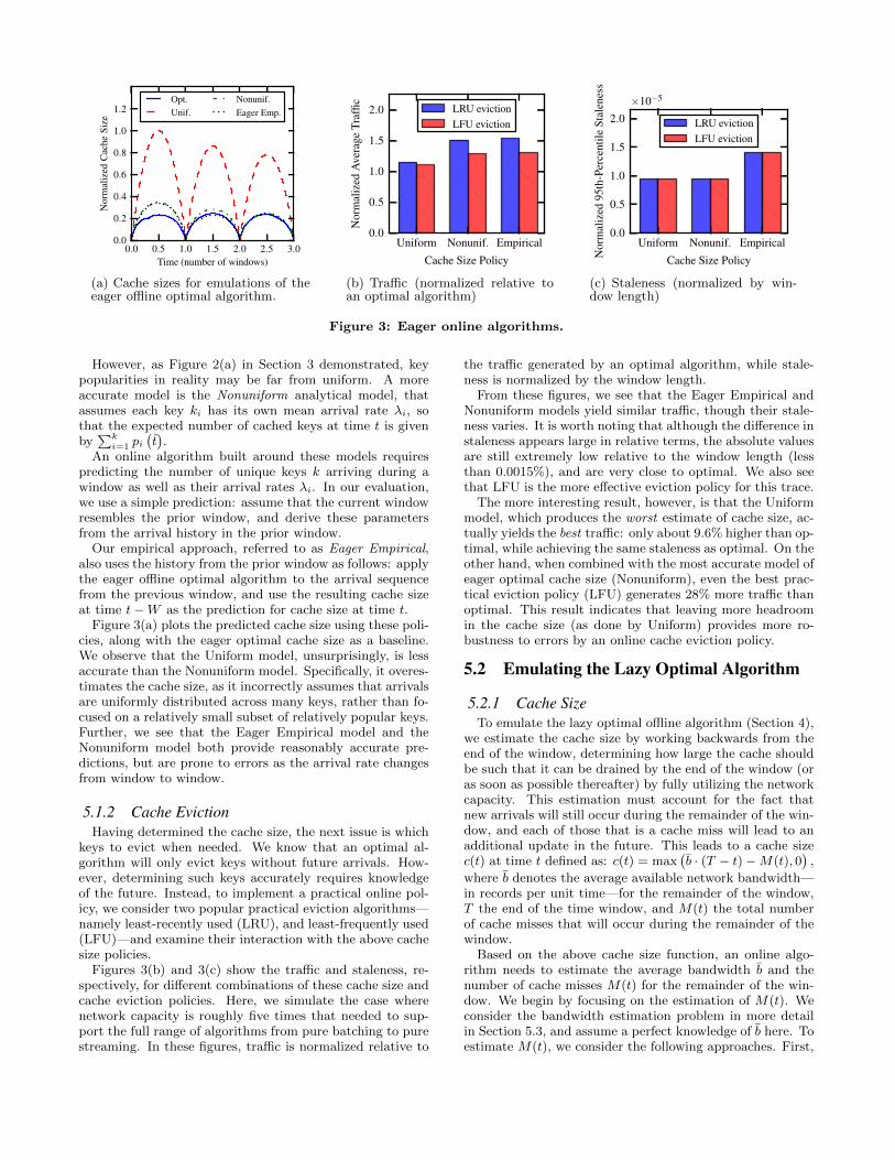
(a) Cache sizes for emulations of theeager offline optimal algorithm.

Uniform Nonunif. Empirical

Cache Size Policy

0.0

0.5

1.0

1.5

2.0

Nor

mal

ized

Ave

rage

Traf

fic LRU evictionLFU eviction

(b) Traffic (normalized relative toan optimal algorithm)

Uniform Nonunif. Empirical

Cache Size Policy

0.0

0.5

1.0

1.5

2.0

Nor

mal

ized

95th

-Per

cent

ileSt

alen

ess

×10−5

LRU evictionLFU eviction

(c) Staleness (normalized by win-dow length)

Figure 3: Eager online algorithms.

However, as Figure 2(a) in Section 3 demonstrated, keypopularities in reality may be far from uniform. A moreaccurate model is the Nonuniform analytical model, thatassumes each key ki has its own mean arrival rate λi, sothat the expected number of cached keys at time t is givenby∑ki=1 pi

(t).

An online algorithm built around these models requirespredicting the number of unique keys k arriving during awindow as well as their arrival rates λi. In our evaluation,we use a simple prediction: assume that the current windowresembles the prior window, and derive these parametersfrom the arrival history in the prior window.

Our empirical approach, referred to as Eager Empirical,also uses the history from the prior window as follows: applythe eager offline optimal algorithm to the arrival sequencefrom the previous window, and use the resulting cache sizeat time t−W as the prediction for cache size at time t.

Figure 3(a) plots the predicted cache size using these poli-cies, along with the eager optimal cache size as a baseline.We observe that the Uniform model, unsurprisingly, is lessaccurate than the Nonuniform model. Specifically, it overes-timates the cache size, as it incorrectly assumes that arrivalsare uniformly distributed across many keys, rather than fo-cused on a relatively small subset of relatively popular keys.Further, we see that the Eager Empirical model and theNonuniform model both provide reasonably accurate pre-dictions, but are prone to errors as the arrival rate changesfrom window to window.

5.1.2 Cache EvictionHaving determined the cache size, the next issue is which

keys to evict when needed. We know that an optimal al-gorithm will only evict keys without future arrivals. How-ever, determining such keys accurately requires knowledgeof the future. Instead, to implement a practical online pol-icy, we consider two popular practical eviction algorithms—namely least-recently used (LRU), and least-frequently used(LFU)—and examine their interaction with the above cachesize policies.

Figures 3(b) and 3(c) show the traffic and staleness, re-spectively, for different combinations of these cache size andcache eviction policies. Here, we simulate the case wherenetwork capacity is roughly five times that needed to sup-port the full range of algorithms from pure batching to purestreaming. In these figures, traffic is normalized relative to

the traffic generated by an optimal algorithm, while stale-ness is normalized by the window length.

From these figures, we see that the Eager Empirical andNonuniform models yield similar traffic, though their stale-ness varies. It is worth noting that although the difference instaleness appears large in relative terms, the absolute valuesare still extremely low relative to the window length (lessthan 0.0015%), and are very close to optimal. We also seethat LFU is the more effective eviction policy for this trace.

The more interesting result, however, is that the Uniformmodel, which produces the worst estimate of cache size, ac-tually yields the best traffic: only about 9.6% higher than op-timal, while achieving the same staleness as optimal. On theother hand, when combined with the most accurate model ofeager optimal cache size (Nonuniform), even the best prac-tical eviction policy (LFU) generates 28% more traffic thanoptimal. This result indicates that leaving more headroomin the cache size (as done by Uniform) provides more ro-bustness to errors by an online cache eviction policy.

5.2 Emulating the Lazy Optimal Algorithm

5.2.1 Cache SizeTo emulate the lazy optimal offline algorithm (Section 4),

we estimate the cache size by working backwards from theend of the window, determining how large the cache shouldbe such that it can be drained by the end of the window (oras soon as possible thereafter) by fully utilizing the networkcapacity. This estimation must account for the fact thatnew arrivals will still occur during the remainder of the win-dow, and each of those that is a cache miss will lead to anadditional update in the future. This leads to a cache sizec(t) at time t defined as: c(t) = max

(b · (T − t)−M(t), 0

),

where b denotes the average available network bandwidth—in records per unit time—for the remainder of the window,T the end of the time window, and M(t) the total numberof cache misses that will occur during the remainder of thewindow.

Based on the above cache size function, an online algo-rithm needs to estimate the average bandwidth b and thenumber of cache misses M(t) for the remainder of the win-dow. We begin by focusing on the estimation of M(t). Weconsider the bandwidth estimation problem in more detailin Section 5.3, and assume a perfect knowledge of b here. Toestimate M(t), we consider the following approaches. First,

0.0 0.5 1.0 1.5 2.0 2.5 3.0Time (number of windows)

0.0

0.2

0.4

0.6

0.8

1.0

1.2N

orm

aliz

edC

ache

Size

OptimalPessim.

OptimisticLazy Emp.

(a) Cache sizes for emulations of thelazy offline optimal algorithm.

PessimisticOptimistic Empirical

Cache Size Policy

0.0

0.2

0.4

0.6

0.8

1.0

1.2

1.4

Nor

mal

ized

Ave

rage

Traf

fic LRU evictionLFU eviction

(b) Traffic (normalized relative toan optimal algorithm)

Pessimistic Optimistic Empirical

Cache Size Policy

0

1

2

3

4

5

6

Nor

mal

ized

95th

-Per

cent

ileSt

alen

ess

×10−3

LRU evictionLFU eviction

(c) Staleness (normalized by win-dow length)

Figure 4: Lazy online algorithms.

we can use a Pessimistic policy, where we assume that allremaining arrivals in the window will be cache misses. Con-

cretely, we estimate M(t) =∫ Tta(τ) dτ where a(t) is the

arrival rate at time t. In practice, this requires the predic-tion of the future arrival rate a(t). In our evaluation, wesimply assume that the future arrival rate is equal to theaverage arrival rate so far in the window.

Another alternative is to use an Optimistic policy, whichassumes that the current cache miss rate will continue forthe remainder of the window. In other words, M(t) =∫ Ttm(τ)a(τ) dτ where m(t) is the miss rate at time t. In our

evaluation, we predict the arrival rate in the same manneras for the Pessimistic policy, and we use an exponentiallyweighted moving average for computing the recent cachemiss rate.

A third approach is the Lazy Empirical policy, which isanalogous to the Eager Empirical approach. It estimates thecache size by emulating the lazy offline optimal algorithm onthe arrivals for the prior window.

Figure 4(a) shows the cache size produced by each of thesepolicies. We see that both the Lazy Empirical and Opti-mistic models closely capture the behavior of the optimalalgorithm in dynamically decreasing the cache size near theend of the window.7 The Pessimistic algorithm, by assum-ing that all future arrivals will be cache misses, decays thecache size more rapidly than the other algorithms.

5.2.2 Cache EvictionWe explore the same eviction algorithms here, namely

LRU and LFU, as we did in Section 5.1.Figures 4(b) and 4(c) show the traffic and staleness, re-

spectively, generated by different combinations of these cachesize and cache eviction policies. We see that LFU againslightly outperforms LRU. More importantly, we see that,regardless of which cache size policy we use, these lazy ap-proaches outperform the best online eager algorithm in termsof traffic. Even the worst lazy online algorithm producestraffic less than 4% above optimal.

The results for staleness, however, show a significant dif-ference between the different policies. We see that by as-suming that all future arrivals will be cache misses, the Pes-simistic policy achieves enough tolerance in the cache size es-

7Note that we are primarily concerned with cache size whileit is decreasing near the end of the window.

0.0% 20.0% 40.0% 60.0% 80.0% 100.0%Network Capacity Overprediction

0.00

0.02

0.04

0.06

0.08

0.10

Nor

mal

ized

95th

-Per

cent

ileSt

alen

ess

LazyHyb. (0.75)Hyb. (0.50)Hyb. (0.25)Eager

Figure 5: Sensitivity of the hybrid algorithms witha range of α values to overpredicting the availablenetwork capacity. Staleness is normalized by win-dow length.

timation, avoiding overloading the network towards the endof the window, and leading to low staleness (below 6× 10−5

for both eviction policies).Based on the results so far, we see that accurately model-

ing the optimal cache size does not yield the best results inpractice. Instead, our algorithms should be lazy, deferringupdates until later in the window, and in choosing how longto defer, they should be pessimistic in their assumptionsabout future arrivals.

5.3 The Hybrid AlgorithmIn the discussion of the lazy online algorithm above, we

assumed perfect knowledge of the future network bandwidthb. In practice, however, if the actual network capacity turnsout to be lower than the predicted value, then too much traf-fic may back up close to the end of the window, potentiallyresulting in high staleness.

Figure 5 shows how staleness increases as the result ofoverpredicting network capacity. Note that the predictedcapacity remains constant, while we vary the actual networkcapacity. The top-most curve corresponds to a lazy onlinealgorithm (Pessimistic + LFU) which is susceptible to veryhigh staleness if it overpredicts network capacity (up to 9.9%of the window length for 100% overprediction).

To avoid this problem, recall Theorem 4, where we ob-served that the eager and lazy optimal algorithms are merelytwo extremes in a family of optimal algorithms. Further, ourresults from Sections 5.1 and 5.2 showed that it is useful to

Eager Hyb. (0.25) Hyb. (0.5) Hyb. (0.75) Lazy

Cache Size Policy

0.0

0.2

0.4

0.6

0.8

1.0

1.2

1.4

Nor

mal

ized

Ave

rage

Traf

fic

Figure 6: Average traffic for hybrid algorithms withseveral values of the laziness parameter α. Traffic isnormalized relative to an optimal algorithm.

add headroom to the accurate cache size estimates: towardsa larger (resp., smaller) cache size in case of the eager (resp.,lazy) algorithm. These insights indicate that a more effec-tive cache size estimate should lie somewhere between theestimates for the eager and lazy algorithms. Hence, we pro-pose a Hybrid algorithm that computes cache size as a lin-ear combination of eager and lazy cache sizes. Concretely,a Hybrid algorithm with a laziness parameter α—denotedby Hybrid(α)—estimates the cache size c(t) at time t as:c(t) = α · cl(t) + (1 − α) · ce(t), where cl(t) and ce(t) arethe lazy and eager cache size estimates, respectively. In ourevaluation, we use the Nonuniform model for the eager andthe Optimistic model for the lazy cache size estimation re-spectively, as these most accurately capture the cache sizesof their respective optimal baselines.

Observing Figure 5 again, we see that as we decrease thelaziness parameter (α) below about 0.5, and use a more ea-ger approach, the risk of bandwidth misprediction is largelymitigated, and the staleness even under significant band-width overprediction remains small.

Note that since predicted network capacity is constant inthis figure, traffic is fixed for each algorithm irrespective ofthe bandwidth prediction error. Figure 6 shows that as weuse a more eager hybrid algorithm, traffic increases. Thisillustrates a tradeoff between traffic and staleness in terms ofachieving robustness to network bandwidth overprediction.A reasonable compromise seems to be a low α value, say0.25. Using this algorithm, traffic is less than 6.0% aboveoptimal, and even when network capacity is overpredicted by100%, staleness remains below 0.19% of the window length.

Overall, we find that a purely eager online algorithm issusceptible to errors by practical eviction policies, while apurely lazy online algorithm is susceptible to errors in band-width prediction. A hybrid algorithm that combines thesetwo approaches provides a good compromise by being morerobust to errors in both arrival process and bandwidth esti-mation.

6. IMPLEMENTATIONWe demonstrate the practicality of our algorithms and ul-

timately their performance by implementing them in ApacheStorm [2]. Our prototype uses a distinct Storm cluster ateach edge, as well as at the center, in order to distribute thework of aggregation. We choose this multi-cluster approachrather than attempting to deploy a single geo-distributedStorm cluster for two main reasons. First, a single global

Storm cluster would require a custom task scheduler in orderto control task placement. Second, and much more critically,Storm was designed and has been optimized for high perfor-mance within a single datacenter; it would not be reasonableto expect it to perform well in a geo-distributed setting char-acterized by high latency and high degrees of compute andbandwidth heterogeneity.

Figure 7 shows the overall architecture, including the edgeand center Storm topologies. We briefly discuss each com-ponent in the order of data flow from edge to center.

Center

SocketReceiver Reorderer StatsCollectorEdgeSummerEdgeSummerEdgeSummerAggregator

Edge

Replayer Reorderer

Logs

EdgeSummerEdgeSummerEdgeSummerAggregator

SocketSender

Figure 7: Aggregation is distributed over ApacheStorm clusters at each edge as well as at the center.

6.1 EdgeData enters our prototype through the Replayer spout.

One instance of this spout runs within each edge, and itis responsible for replaying timestamped logs from a file,reproducing the original pattern of interarrival times. Inorder to allow us to explore different stream arrival rates, theReplayer takes a speedupFactor parameter, which dictateshow much to speed up or slow down the log replay.

Each line of the logs is parsed using a query-specific pars-ing function, which produces a triple of (timestamp, key,

value). We leverage Twitter’s Algebird8 library to general-ize over a broad class of aggregations, so the only restrictionon value types is that they must have an Algebird Semigroup

instance. This is already satisfied for many practical aggre-gations (e.g., integer sum, unique count via HyperLogLog,etc.), and implementing a custom Semigroup is straightfor-ward. The Replayer emits these records downstream, andalso periodically emits punctuation messages. Carrying onlya timestmap, these punctuation messages simply denote thatno messages with earlier timestamps will be sent in the fu-ture. The frequency of these punctuations is user-specified,though it is required that one be sent to mark the end ofeach time window.

The next step in the dataflow is the Aggregator bolt, forwhich one or more tasks run at each cluster. Each task isresponsible for aggregating a hash-partitioned subset of thekey space, and applying a cache size and eviction policy todetermine when to transfer partial aggregates to the center.Each task maintains an in-memory key-value map, and usesthe Algebird library to aggregate values for a given key. Wegeneralize over a broad range of eviction policies by orderingkeys using a priority queue with an efficient changePriorityimplementation, and consulting this priority queue to deter-mine the next victim key when it becomes necessary. Bydefining priority as a function of key, value, existing priority

8https://github.com/twitter/algebird

(if any) and the time that the key was last updated in themap, we can capture a broad range of algorithms includingLRU and LFU.

The Aggregator also maintains a cache size function, whichmaps from time within the window to a cache size. Thisfunction can be changed at runtime in order to support im-plementing arbitrary dynamic sizing policies. Specifically, aconcrete Aggregator instance can install callback functionsto be invoked upon the arrival of records or punctuations.This mechanism can be used, for example, to update thecache size function based on arrival rate and miss rate asin our Lazy Pessimistic algorithm, or to record the arrivalhistory for one window and use this history to compute thesize function for the next window, as in the Eager Empiricalalgorithm. For our experiments, we use this mechanism toimplement a cache size policy that learns the eager optimaleviction schedule after processing the log trace once.

The Aggregator tasks send their output to a single in-stance of the Reorderer bolt. This bolt is responsible fordelaying records as needed in order to maintain punctua-tion semantics. Data then flows into the SocketSender bolt,which connects to the central cluster at startup, and has theresponsibility of serializing and transmitting partial aggre-gates downstream to the center using TCP sockets. ThisSocketSender also maintains an estimate of network band-width to the center, and periodically emits these estimatesupstream to Aggregator instances for use in defining theircache size functions. Our bandwidth estimation is basedon simple measurements of the rate at which messages canbe sent over the network. For a more reliable prediction,we could employ lower-level techniques [7], or even externalmonitoring services [26].

6.2 CenterAt the center, data follows largely the reverse order. First,

the SocketReceiver spout is responsible for deserializingpartial aggregates and punctuations and emitting them down-stream into a Reorderer, where the streams from multipleedges are synchronized. From there, records flow into thecentral Aggregator, each task of which is responsible for per-forming the final aggregation over a hash-partitioned subsetof the key space. Upon completing aggregation for a win-dow, these central Aggregator tasks emit summary metricsincluding traffic and staleness, and these metrics are sum-marized by the final StatsCollector bolt.

Note that our prototype achieves at-most-once deliverysemantics. Storm’s acking mechanisms can be used to im-plement at-least-once semantics, and exactly-once seman-tics can be achieved by employing additional checks to filterduplicate updates, though we have not implemented thesemeasures.

7. EXPERIMENTAL EVALUATIONTo evaluate the performance of our algorithms in a real

geo-distributed setting, we deploy our Apache Storm archi-tecture on the PlanetLab testbed. Our PlanetLab deploy-ment uses a total of eleven nodes (64 total cores) spanningseven sites. Central aggregation is performed using a Stormcluster at a single node at princeton.edu9. Edge locations

9We originally employed multiple nodes at the center, butwere forced to confine our central aggregation to a singlenode due to PlanetLab’s restrictive limitations on daily net-

include csuohio.edu, uwaterloo.ca, yale.edu, washing-

ton.edu, ucla.edu, and wisc.edu. Bandwidth from edgeto center varies from as low as 4.5Mbps (csuohio.edu) to ashigh as 150Mbps (yale.edu), based on iperf. To simulatestreaming data, each edge replays a geographic partition ofthe CDN log data described in Section 3. To explore theperformance of our algorithms under a range of workloads,we use the three diverse queries described in Table 1, andwe replay the logs at both low and high (8x faster than low)rates. Note that for confidentiality purposes, we do not dis-close the actual replay rates, and we present staleness andtraffic results normalized relative to the window length andoptimal traffic, respectively.

7.1 Aggregation using a Single EdgeAlthough our work is motivated by the general case of

multiple edges, our algorithms were developed based on anin-depth study of the interaction between a single edge andcenter. We therefore begin by studying the real-world per-formance of our hybrid algorithm when applied at a singleedge. Following the rationale from Section 5.3, we choose alaziness parameter of α = 0.25 for this initial experiment,though we will study the tradeoffs of different parametervalues shortly.

Compared to the extremes of pure batching and purestreaming, as well as an optimal algorithm based on a pri-ori knowledge of the data stream, our algorithm performsquite well. Figures 8(a) and 8(b) show that our hybrid al-gorithm very effectively exploits the opportunity to reducebandwidth relative to streaming, yielding traffic less than2% higher than the optimal algorithm. At the same time,our hybrid algorithm is able to reduce staleness by 65% rel-ative to a pure batching algorithm.

7.2 Scaling to Multiple EdgesIn order to understand how well our algorithm scales be-

yond a single edge, we partition the log data over threegeo-distributed edges. We replay the logs at both low andhigh rates, and for each of the large, medium, and small

queries10. As Figures 9(a) and 9(b) demonstrate, our hy-brid algorithm performs well throughout. It is worth notingthat the edges apply their cache size and cache eviction poli-cies based purely on local information, without knowledge ofthe decisions made by the other edges, except indirectly viathe effect that those decisions have on the available networkbandwidth to the center.

Performance is generally more favorable for our algorithmfor the large and medium queries than for the small query.The reason is that, for these larger queries, while edge aggre-gation reduces communication volume, there is still a greatdeal of data to transfer from the edges to the center. Stal-eness is quite sensitive to precisely when these partial ag-gregates are transferred, and our algorithms work well inscheduling this communication. For the small query, on theother hand, edge aggregation is extremely effective in re-ducing data volumes, so much so that there is little risk indelaying communication until the end of the window. Forqueries that aggregate extremely well, batching is a promis-

work bandwidth usage that was quickly exhausted by thecommunication between Storm workers.

10We do not present the results for large-high because theamount of traffic generated in these experiments could notbe sustained within the PlanetLab bandwidth limits.

Batching Hybrid(0.25) Streaming Optimal

Algorithm

0.0

0.5

1.0

1.5

2.0

2.5

3.0

3.5

4.0

Nor

mal

ized

Mea

nTr

affic

(a) Mean traffic (normalized relative to an opti-mal algorithm).

Batching Hybrid(0.25) Streaming Optimal

Algorithm

0.00

0.05

0.10

0.15

0.20

Nor

mal

ized

Med

ian

Stal

enes

s

(b) Median staleness (normalized by windowlength).

Figure 8: Performance for batching, streaming, optimal, and our hybrid algorithm for the large query witha low stream arrival rate using a one-edge Apache Storm deployment on PlanetLab.

Lg/Low Md/Low Md/High Sm/Low Sm/High

Query/Arrival Rate

0

1

2

3

4

5

Nor

mal

ized

Mea

nTr

affic

BatchingHybrid(0.25)StreamingOptimal

(a) Mean traffic (normalized relative to an op-timal algorithm). Normalized traffic values forstreaming are truncated, as they range as high as164.

Lg/Low Md/Low Md/High Sm/Low Sm/High

Query/Arrival Rate

0.000.010.020.030.040.050.060.070.08

Nor

mal

ized

Med

ian

Stal

enes

s BatchingHybrid(0.25)StreamingOptimal

(b) Median staleness (normalized by windowlength).

Figure 9: Performance for batching, streaming, optimal, and our hybrid algorithm for a range of queries andstream arrival rates using a three-edge Apache Storm deployment on PlanetLab.

ing algorithm, and we do not necessarily outperform batch-ing. The advantage of our algorithm over batching is there-fore its broader applicability: the Hybrid algorithm performsroughly as well as batching for small queries, and signifi-cantly outperforms it for large queries.

We continue by further partitioning the log data across atotal of six geo-distributed edges. Given the higher aggre-gate compute and network capacity of this deployment, wefocus on the large query at both low and high arrival rates.From Figure 10(a), we can again observe that our hybrid al-gorithm yields near-optimal traffic. We can also observe animportant effect of stream arrival rate: all else equal, a highstream arrival rate lends itself to more thorough aggregationat the edge. This is evident in the higher normalized trafficfor streaming with the high arrival rate than with the lowarrival rate.

In terms of staleness, Figure 10(b) shows that our algo-rithm performs well for the high arrival rate, where the net-work capacity is more highly constrained, and staleness istherefore more sensitive to the particular scheduling algo-rithm. At the low arrival rate, we see that our hybrid al-gorithm performs slightly worse than batching, though inabsolute terms this difference is quite small. Our hybrid al-gorithm generates higher staleness than streaming, but doesso at a much lower traffic cost. Just as with the three-edgecase, we again see that, where a large opportunity exists, ouralgorithm exploits it, and where an extreme algorithm such

as batching already suffices, our algorithm remains compet-itive.

7.3 Effect of Laziness ParameterIn Section 5.3, we observed that a purely eager algorithm

is vulnerable to mispredicting which keys will receive furtherarrivals, while a purely lazy algorithm is vulnerable to over-predicting network bandwidth. This motivated our hybridalgorithm, which uses a linear combination of eager and lazycache size functions. We explore the real-world tradeoffs ofusing a more or less lazy algorithm by running experimentswith the large query at a low replay rate over three edgeswith laziness parameter α ranging from 0 through 1.0 bysteps of 0.25. As expected based on our simulation results,Figure 11(a) shows that α has little effect on traffic whenit exceeds about 0.25. Somewhere below this value, the im-perfections of practical cache eviction algorithms (LRU inour implementation) begin to manifest. More specifically,at α = 0, the hybrid algorithm reduces to a purely eageralgorithm, which makes eviction decisions well ahead of theend of the window, and often chooses the wrong victim.By introducing even a small amount of laziness, say withα = 0.25, this effect is largely mitigated.

Figure 11(b) shows the opposite side of this tradeoff: alazier algorithm runs a higher risk of deferring communica-tion too long, in turn leading to higher staleness. Based onstaleness alone, a more eager algorithm is better. Based onthe shape of these trends, we have chosen to use α = 0.25

Lg/Low Lg/High

Query/Arrival Rate

0

1

2

3

4

5

Nor

mal

ized

Mea

nTr

affic

BatchingHybrid(0.25)StreamingOptimal

(a) Mean traffic (normalized relative to an opti-mal algorithm).

Lg/Low Lg/High

Query/Arrival Rate

0.00

0.05

0.10

0.15

0.20

Nor

mal

ized

Med

ian

Stal

enes

s BatchingHybrid(0.25)StreamingOptimal

(b) Median staleness (normalized by windowlength).

Figure 10: Performance for batching, streaming, optimal, and our hybrid algorithm for the large query withlow and high stream arrival rates using a six-edge Apache Storm deployment on PlanetLab.

throughout our experiments, but this may not be the opti-mal value. Further study would be necessary to determinean optimal value of α, and this optimal choice may in factdepend on the relative importance of minimizing stalenessversus minimizing traffic.

8. RELATED WORKAggregation: Aggregation is a key operator in analytics,and grouped aggregation is supported by many data-parallelprogramming models [8, 12, 27]. Larson et al. [17] explorethe benefits of performing partial aggregation prior to a joinoperation, much as we do prior to network transmission.While they also recognize similarities to caching, they con-sider only a fixed-size cache, whereas our approach uses adynamically varying cache size. In sensor networks, aggre-gation is often performed over a hierarchical topology toimprove energy efficiency and network longevity [18, 24],whereas we focus on cost (traffic) and information quality(staleness). Amur et al. [6] study grouped aggregation, fo-cusing on the design and implementation of efficient datastructures for batch and streaming computation. They dis-cuss tradeoffs between eager and lazy aggregation, but donot consider the effect on staleness, a key performance met-ric in our work.Streaming systems: Numerous streaming systems [5, 9,22, 28] have been proposed in recent years. These systemsprovide many useful ideas for new analytics systems to buildupon, but they do not fully explore the challenges that we’vedescribed here, in particular how to achieve high qualityresults (low staleness) at low cost (low traffic).Wide-area computing: Wide-area computing has receivedincreased research attention in recent years, due in part tothe widening gap between data processing and communica-tion costs. Much of this attention has been paid to batchcomputing [25]. Relatively little work on streaming compu-tation has focused on wide-area deployments, or associatedquestions such as where to place computation. Pietzuch etal. [20] optimize operator placement in geo-distributed set-tings to balance between system-level bandwidth usage andlatency. Hwang et al. [16] rely on replication across the widearea in order to achieve fault tolerance and reduce stragglereffects. JetStream [23] considers wide-area streaming com-putation, but unlike our work, assumes that it is alwaysbetter to push more computation to the edge.

Optimization tradeoffs: LazyBase [10] provides a mech-anism to trade off increased staleness for faster query re-sponse in the case of ad-hoc queries. BlinkDB [4] and Jet-Stream [23] provide mechanisms to trade off accuracy withresponse time and bandwidth utilization, respectively. Ourfocus is on jointly optimizing both network traffic and stale-ness. Das et al. [11] have studied the impact of batch inter-vals on latency and throughput. While their work focuses onsetting batching intervals, we study scheduling at the muchfiner granularity of individual aggregates.

9. CONCLUSIONIn this paper, we focused on optimizing the important

primitive of windowed grouped aggregation in a wide-areastreaming analytics setting on two key metrics: WAN traf-fic and staleness. We presented a family of optimal offlinealgorithms that jointly minimize both staleness and traffic.Using this as a foundation, we developed practical online ag-gregation algorithms based on the observation that groupedaggregation can be modeled as a caching problem where thecache size varies over time. We explored a range of onlinealgorithms ranging from eager to lazy in terms of how soonthey send out updates. We found that a hybrid online algo-rithm works best in practice, as it is robust to a wide rangeof network constraints and estimation errors. We demon-strated the practicality of our algorithms through an im-plementation in Apache Storm, deployed on the PlanetLabtestbed. The results of our experiments, driven by workloadsderived from anonymized traces of Akamai’s web analyticsservice, showed that our online aggregation algorithms per-form close to the optimal algorithms for a variety of systemconfigurations, stream arrival rates, and query types.

10. ACKNOWLEDGMENTSThe authors would like to acknowledge NSF Grant CNS-

1413998, and an IBM Faculty Award, which supported thisresearch.

11. REFERENCES[1] PlanetLab. http://planet-lab.org/, 2015.

[2] Storm, distributed and fault-tolerant realtimecomputation. http://storm.apache.org/, 2015.

[3] M. Adler, R. K. Sitaraman, and H. Venkataramani.Algorithms for optimizing the bandwidth cost of

0 0.25 0.5 0.75 1

α

0.0

0.5

1.0

1.5N

orm

aliz

edM

ean

Traf

fic

(a) Mean traffic (normalized relative to an opti-mal algorithm).

0 0.25 0.5 0.75 1

α

0.000

0.005

0.010

0.015

0.020

0.025

Nor

mal

ized

Med

ian

Stal

enes

s

(b) Median staleness (normalized by windowlength).

Figure 11: Effect of laziness parameter α using a three-edge Apache Storm deployment on PlanetLab withquery large.

content delivery. Computer Networks,55(18):4007–4020, Dec. 2011.

[4] S. Agarwal et al. BlinkDB: queries with boundederrors and bounded response times on very large data.In Proc. of EuroSys, pages 29–42, 2013.

[5] T. Akidau et al. MillWheel: Fault-tolerant streamprocessing at internet scale. Proc. of VLDB Endow.,6(11):1033–1044, Aug. 2013.

[6] H. Amur et al. Memory-efficient groupby-aggregateusing compressed buffer trees. In Proc. of SoCC, 2013.

[7] J. Bolliger and T. Gross. Bandwidth monitoring fornetwork-aware applications. In Proc. of HPDC, pages241–251, 2001.

[8] O. Boykin, S. Ritchie, I. O’Connel, and J. Lin.Summingbird: A framework for integrating batch andonline mapreduce computations. In Proc. of VLDB,volume 7, pages 1441–1451, 2014.

[9] S. Chandrasekaran et al. TelegraphCQ: Continuousdataflow processing for an uncertain world. In CIDR,2003.

[10] J. Cipar, G. Ganger, K. Keeton, C. B. Morrey, III,C. A. Soules, and A. Veitch. LazyBase: tradingfreshness for performance in a scalable database. InProc. of EuroSys, pages 169–182, 2012.

[11] T. Das, Y. Zhong, I. Stoica, and S. Shenker. Adaptivestream processing using dynamic batch sizing. InProc. of SoCC, pages 16:1–16:13, 2014.

[12] J. Gray et al. Data cube: A relational aggregationoperator generalizing group-by, cross-tab, andsub-totals. Data Min. Knowl. Discov., 1(1):29–53,Jan. 1997.

[13] A. Greenberg, J. Hamilton, D. A. Maltz, and P. Patel.The cost of a cloud: Research problems in data centernetworks. SIGCOMM Comput. Commun. Rev.,39(1):68–73, Dec. 2008.

[14] B. Heintz, A. Chandra, and R. K. Sitaraman.Optimizing grouped aggregation in geo-distributedstreaming analytics. Technical Report TR 15-001,Department of Computer Science, University ofMinnesota, 2015.

[15] B. Heintz, A. Chandra, and R. K. Sitaraman. Towardsoptimizing wide-area streaming analytics. In Proc. ofthe 2nd IEEE Workshop on Cloud Analytics, 2015.

[16] J.-H. Hwang, U. Cetintemel, and S. Zdonik. Fast andhighly-available stream processing over wide areanetworks. In Proc. of ICDE, pages 804–813, 2008.

[17] P.-A. Larson. Data reduction by partialpreaggregation. In Proc. of ICDE, pages 706–715,2002.

[18] S. Madden, M. J. Franklin, J. M. Hellerstein, andW. Hong. TAG: A Tiny AGgregation service forad-hoc sensor networks. In Proc. of OSDI, 2002.

[19] E. Nygren, R. K. Sitaraman, and J. Sun. The akamainetwork: a platform for high-performance internetapplications. SIGOPS Oper. Syst. Rev., 44(3):2–19,Aug. 2010.

[20] P. Pietzuch et al. Network-aware operator placementfor stream-processing systems. In Proc. of ICDE, 2006.

[21] S. Podlipnig and L. Boszormenyi. A survey of webcache replacement strategies. ACM Comput. Surv.,35(4):374–398, Dec. 2003.

[22] Z. Qian et al. TimeStream: reliable streamcomputation in the cloud. In Proc. of EuroSys, pages1–14, 2013.

[23] A. Rabkin, M. Arye, S. Sen, V. S. Pai, and M. J.Freedman. Aggregation and degradation in JetStream:Streaming analytics in the wide area. In Proc. ofNSDI, pages 275–288, 2014.

[24] R. Rajagopalan and P. Varshney. Data-aggregationtechniques in sensor networks: A survey. IEEECommunications Surveys Tutorials, 8(4):48–63, 2006.

[25] A. Vulimiri, C. Curino, B. Godfrey, K. Karanasos, andG. Varghese. WANalytics: Analytics for ageo-distributed data-intensive world. CIDR 2015,January 2015.

[26] R. Wolski, N. T. Spring, and J. Hayes. The networkweather service: a distributed resource performanceforecasting service for metacomputing. Future Gener.Comput. Syst., 15(5-6):757–768, Oct. 1999.

[27] Y. Yu, P. K. Gunda, and M. Isard. Distributedaggregation for data-parallel computing: interfacesand implementations. In Proc. of SOSP, pages247–260, 2009.

[28] M. Zaharia, T. Das, H. Li, T. Hunter, S. Shenker, andI. Stoica. Discretized streams: Fault-tolerantstreaming computation at scale. In Proc. of SOSP,pages 423–438, 2013.