Optimizing Cost and Performance for Content MultihomingHongqiang Harry Liu� Ye Wang� Yang Richard Yang�× Hao Wang† Chen Tian�

�Yale University †Google ×SplendorStream{hongqiang.liu, ye.wang, yang.r.yang, tian.chen}@yale.edu wanghao@google.com

ABSTRACTMany large content publishers use multiple content distribution net-works to deliver their content, and many commercial systems havebecome available to help a broader set of content publishers to ben-efit from using multiple distribution networks, which we refer toas content multihoming. In this paper, we conduct the first sys-tematic study on optimizing content multihoming, by introducingnovel algorithms to optimize both performance and cost for contentmultihoming. In particular, we design a novel, efficient algorithmto compute assignments of content objects to content distributionnetworks for content publishers, considering both cost and perfor-mance. We also design a novel, lightweight client adaptation algo-rithm executing at individual content viewers to achieve scalable,fine-grained, fast online adaptation to optimize the quality of expe-rience (QoE) for individual viewers. We prove the optimality of ouroptimization algorithms and conduct systematic, extensive evalua-tions, using real charging data, content viewer demands, and per-formance data, to demonstrate the effectiveness of our algorithms.We show that our content multihoming algorithms reduce publish-ing cost by up to 40%. Our client algorithm executing in browsersreduces viewer QoE degradation by 51%.

Categories and Subject Descriptors: C.2.3 [Computer Commu-nication Networks]: Network Operations.

Keywords: Content Delivery, Multiple CDNs, Optimization.

1. INTRODUCTIONMany content publishers on the Internet use multiple content dis-

tribution networks (CDNs) to distribute and cache their digital con-tent. We refer to content publishing using multiple content distri-bution networks as content multihoming. In our recent survey, wefound that all major content publishers such as Netflix, Hulu, Mi-crosoft, Apple, Facebook, and MSNBC use content multihoming.

Content publishers adopt content multihoming to aggregate thediversity of individual CDN providers on features, performance andcommitment [7]. For example, one CDN may provide good cov-erage for locations 1 and 2, whereas another CDN provides goodcoverage for locations 2 and 3. To deliver content to viewers fromall three locations, a content publisher may need to use both CDNs.

Given the wide usage and potential benefits of content multi-homing, many commercial systems supporting content multihom-ing have recently been deployed (e.g., [9, 11, 16, 17, 21, 27]), sothat more content publishers can benefit from content multihoming.However, these commercial products either use ad hoc approachesor do not provide details on their designs. No previous studies onhow to effectively utilize content multihoming are known.

In this paper, we attempt to provide a framework and a set ofnovel algorithms to optimize the benefits of content multihoming.

Permission to make digital or hard copies of all or part of this work forpersonal or classroom use is granted without fee provided that copies arenot made or distributed for profit or commercial advantage and that copiesbear this notice and the full citation on the first page. To copy otherwise, torepublish, to post on servers or to redistribute to lists, requires prior specificpermission and/or a fee.SIGCOMM’12, August 13–17, 2012, Helsinki, Finland.Copyright 2012 ACM 978-1-4503-1419-0/12/08 ...$15.00.

We ask a simple question: Given that content multihoming allows acontent object to be delivered from multiple CDNs, which CDN(s)should a content publisher use to deliver each object to each con-tent viewer requesting this object, so that the publisher optimizesits benefits from content multihoming? This question is the keyto efficiently utilizing content multihoming, since its solutions canbe implemented directly with the flexible request routing mecha-nisms (e.g., DNS CNAME, HTTP Redirect from servers, and clientscripts in end hosts) in modern content delivery infrastructures.

An answer to this simple question, however, is not immediatelyobvious. Consider the current common approach of choosing, foreach content viewer, the best performing CDN among all candidateCDNs. This approach, despite its simplicity, has multiple issues.First, although the chosen CDN may provide the highest level ofperformance, for example, satisfying that 99% viewers do not seequality of experience (QoE) degradation, the cost of the chosenCDN can be much higher than another CDN with a slightly lower,but still high enough level of 95%. Second, there are often multi-ple CDNs with comparable and sufficient levels of performance ata given region, e.g., in US. One common approach to break ties insuch cases is to pick the CDN with the lowest cost. However, thecosts of CDNs, in particular, pay-as-you-go CDNs such as Ama-zon CloudFront, are volume based and non-linear. The cost of oneobject assignment depends on the other assignments. Third, thereare locations where even the best performing CDN falls short. Forexample, a content publisher may have a QoE target of 95%, butthe best performing CDN at some location achieves only 90%.

In this paper, we answer the preceding question by designingtwo algorithms: (1) an efficient optimization algorithm executingat content publisher to compute content distribution guidance, and(2) a simple algorithm executing at individual content viewers tofollow the guidance with local adaptation. Either algorithm can bedeployed alone, but together they benefit the most.

Specifically, the publisher optimization algorithm, named CMO,computes CDN assignments considering many real factors: non-linear, multi-region CDN traffic charging, per-request charging, con-tent licensing restrictions, CDN feature availability, and CDN per-formance variations. The CMO algorithm is novel and highly ef-ficient. For example, when considering traffic cost only, the com-plexity of CMO is polynomial and independent of the number ofcontent objects, whereas the complexity of simple enumeration isexponential in the number of content objects.

The local viewer algorithm provides a capability for a contentviewer to make efficient usage of multiple servers from multipleCDNs, with a preference ordering on the usage of CDN edge serversprovided by the content publisher. Inspired by TCP AIMD andusing a simple prioritized assignment mechanism, the algorithmadapts the usage of multiple CDNs, achieving a performance levelthat no single CDN/server can achieve alone.

We implement both of the algorithms and conduct systematic,extensive evaluations using real charging data, content viewer de-mands, and CDN performance to demonstrate the effectiveness ofour algorithms. We show that our content multihoming algorithmsreduce publishing cost by up to 40%. Our implementation of theclient algorithm running in Adobe Flash enabled browsers reducesviewer QoE degradation by 51%.

371

2. RELATED WORKThe importance of content multihoming has led to substantial

industrial related work. We divide the industrial efforts into threecategories [7]. The first category is software systems which wename CDN switchers (e.g., [1, 21]) and integrators (e.g., [19, 27].For example, the One Pica Image CDN extension [21] of the Ma-gento Commerce platform provides an API to support the inte-gration with multiple CDNs, including Amazon S3, Coral CDN,Mosso/Rackspace Cloud Files, and any CDN server or service thatsupports FTP, FTPS, or SFTP. Their objective, however, is not onthe algorithms to effectively use multiple CDNs, but rather on us-ability issues such as seamless switching from one CDN providerto another. Commercial systems such as [19, 27] provide CDN ser-vices based on aggregation of multiple CDNs. They can benefitfrom using our algorithms.

Going beyond the CDN switchers and integrators is a categoryof systems named CDN Load balancers. There are many CDNload balancers commercially available, including Cotendo CDNbalancer, LimeLight traffic load balancer, Level 3 intelligent trafficmanagement, and Dyn CDN manager. Some of these systems of-fer quite flexible rules to split CDN traffic among multiple CDNs.For example, Cotendo CDN balancer supports rules with weightedallocation, geographic location, geographic distance, time of day,and any combination. In particular, the weighted allocation ruleallows a publisher to specify: x percent to CDN one, y percent toCDN two, and so on. A key missing component of these existingsystems, however, is the key algorithms to compute the allocation(e.g., the percentages). Hence, the output of our optimizer can beused to configure these systems.

There are also client based CDN load balancers. One interest-ing example is Conviva [9], whose video player plug-in performscontinuous video quality monitoring, and could perform automaticCDN and/or source server switching during video playback. Theexact details of their algorithm, however, are unknown.

A third category of related industrial efforts is CDN intercon-nect. In [20], a CDN interconnect (CDNi) architecture has beenproposed so that a content publisher contracts with a few upstreamCDNs, who may delegate some requests to downstream CDNs. Thedelegation relationship can be recursive to form a directional dele-gation graph, and all of the involved CDNs are said to form a CDNfederation [5]. Our algorithms can be extended to the CDNi settingby considering a set of connected CDNs as a single logical CDN.

So far content multihoming has not been a focus of academicresearch. A related recent academic work is a measurement studyof Netflix [2]. The paper shows that similar to many content pub-lishers, Netflix uses content multihoming. The paper conducts ameasurement study and shows that there are indeed potential per-formance benefits of using content multihoming.

There has been some recent studies on intra-CDN optimizationswhich can be used in conjunction with content multihoming. Theauthors of [3, 22, 23, 24] study how CDNs can utilize informationon load of edge servers, network conditions, and locations/bandwidthof clients to improve CDN request routing. Our work complementsthese studies by optimizing the assignment of contents into CDNs.

We refer to our system as content multihoming to draw an anal-ogy with traditional Internet multihoming (e.g., [13]). However,content multihoming is quite different from traditional ISP multi-homing. For example, while ISPs typically have a uniform pricebased on traffic, CDNs charge customers by regions.

3. BACKGROUND AND NOTATIONSWe start by introducing the background and notations. Table 1

provides a reference for the major notations used in this paper.There are three key types of entities being managed in content

multihoming: (1) content objects; (2) viewers of contents; (3) dis-tribution networks that cache contents from origin networks to servecontent viewers.Content object: A content publisher can have a large number ofcontent objects such as videos and images. Let N denote the totalnumber of content objects. An object has many properties. In thecontext of content distribution, the performance requirement, thesize, and the popularity of an object are its key properties [4]. Letsi be the size of object i. We introduce object popularity when wenext introduce content viewers.

N Number of content objects.K Number of CDNs.A Set of fine-grained location areas.si Size of object i.nai Number of requests for object i from area a.ia Location object: object i requested from location area a.αrk Set of location areas served by charging region r of CDN k.trk Charging volume of CDN k at its charging region r.Crk() Charging function of CDN k for its charging region r.Fk Set of location objects that CDN k can serve.

pai,kCDN k’s performance for object i at location area a:fraction of times CDN k can deliver ia with sufficient QoE.

xai,k CDN guidance: fraction of nai requests directed to CDN k.ψk CDN assignment: set of location objects assigned to CDN k.

Table 1: Summary of key notations.

Content viewer (client): There can be a large number of contentviewers requesting content objects. These content viewers can bedistributed across multiple geographical areas. The specific geo-graphical areas depend on the particular requirements of a contentpublisher. For generality and conceptual clarity, let A be the set ofall geographical areas, say all cities or countries. Note that in thischallenging general case the size of A can be large, on the order ofthousands. Let a ∈ A denote a location area.

The popularity of an object among content viewers is locationdependent [12]. Let nai denote the number of times that object iwillbe requested, during a time interval (say a month), from contentviewers located at location area a.

We also use nai to encode licensing restrictions that a contentpublisher often needs to enforce in practice. Specifically, if contentviewers from a location area a should not receive a content objecti, nai should be 0.

Content distribution network (CDN): A key reason of contentmultihoming is to aggregate the capability-geography expertise ofdifferent CDNs, as different CDNs can have quite different perfor-mance and cost characteristics, at different geographic regions. Onthe other hand, as we will see, such differences are a major sourceof intrinsic complexity when optimizing content multihoming. Inthis paper, we assume that the set of CDNs is given. Let K be thenumber of CDNs, and we use k and j to index individual CDNs.

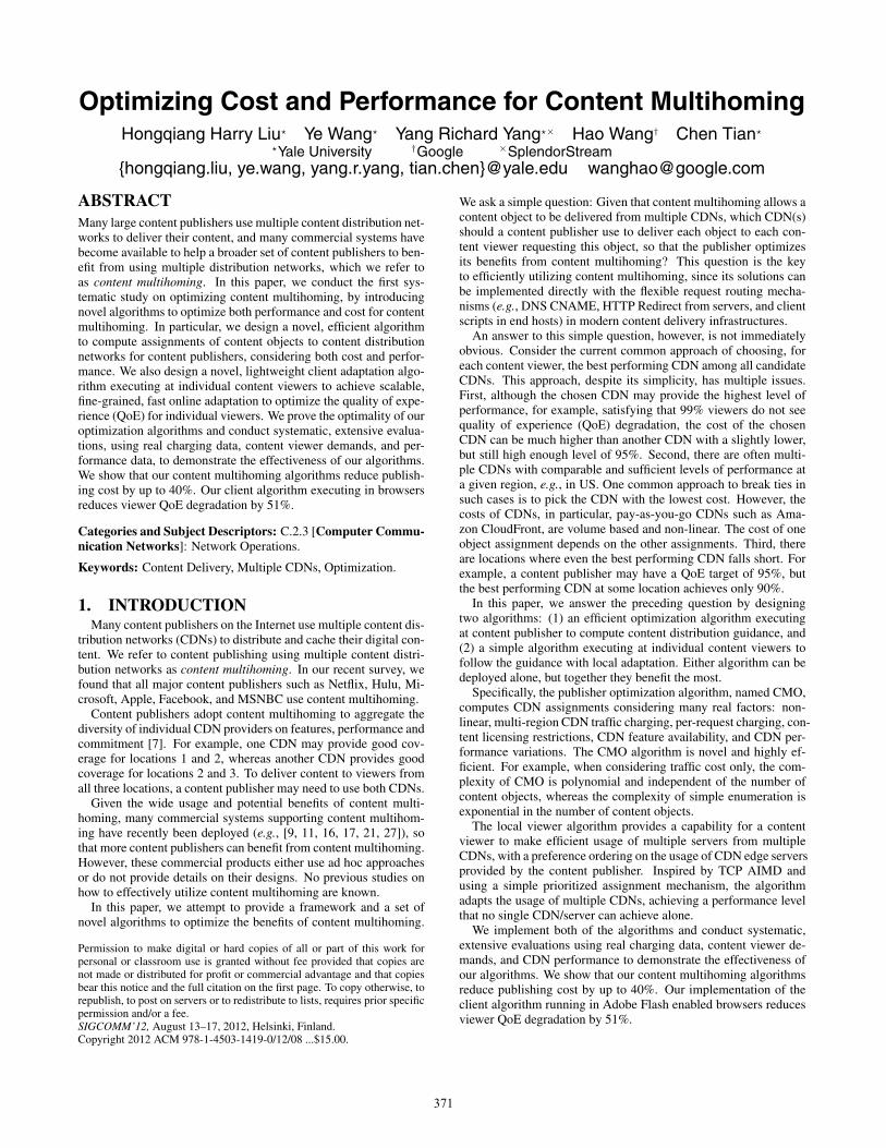
First consider performance. Figure 1 shows the edge server foot-prints of three real CDNs: Amazon CloudFront, MaxCDN and Chi-naCache. When a content viewer from a location area a requests acontent object through CDN k, a well designed CDN will choosean edge server (or several servers) that is close to a to serve therequest, since a short latency from edge servers to end users is typ-ically needed to achieve good content delivery performance [15].Comparing the geographical footprints of the three CDNs shownin Figure 1, one can anticipate that CloudFront and MaxCDN aremore likely to provide better performance in US and Europe, whileChinaCache may perform well in China. None of the three coversregions such as Russia and Africa.

To quantify the performance, we conduct performance measure-ments using 600 PlanetLab nodes at different locations to requestcontent objects from three CDNs (CloudFront, MaxCDN, and Liq-uid Web). Since performance metrics are dependent on the content

372

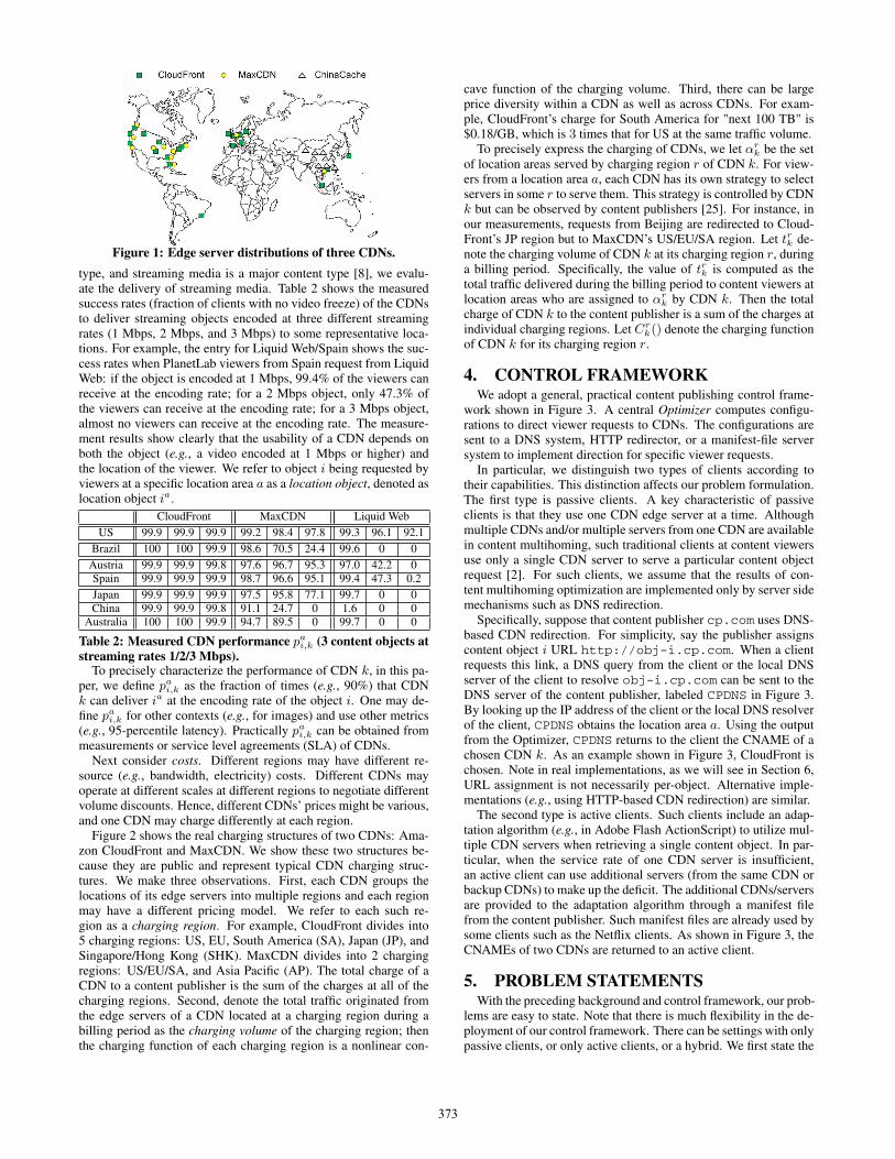
Figure 1: Edge server distributions of three CDNs.

type, and streaming media is a major content type [8], we evalu-ate the delivery of streaming media. Table 2 shows the measuredsuccess rates (fraction of clients with no video freeze) of the CDNsto deliver streaming objects encoded at three different streamingrates (1 Mbps, 2 Mbps, and 3 Mbps) to some representative loca-tions. For example, the entry for Liquid Web/Spain shows the suc-cess rates when PlanetLab viewers from Spain request from LiquidWeb: if the object is encoded at 1 Mbps, 99.4% of the viewers canreceive at the encoding rate; for a 2 Mbps object, only 47.3% ofthe viewers can receive at the encoding rate; for a 3 Mbps object,almost no viewers can receive at the encoding rate. The measure-ment results show clearly that the usability of a CDN depends onboth the object (e.g., a video encoded at 1 Mbps or higher) andthe location of the viewer. We refer to object i being requested byviewers at a specific location area a as a location object, denoted aslocation object ia.

CloudFront MaxCDN Liquid WebUS 99.9 99.9 99.9 99.2 98.4 97.8 99.3 96.1 92.1

Brazil 100 100 99.9 98.6 70.5 24.4 99.6 0 0Austria 99.9 99.9 99.8 97.6 96.7 95.3 97.0 42.2 0Spain 99.9 99.9 99.9 98.7 96.6 95.1 99.4 47.3 0.2Japan 99.9 99.9 99.9 97.5 95.8 77.1 99.7 0 0China 99.9 99.9 99.8 91.1 24.7 0 1.6 0 0

Australia 100 100 99.9 94.7 89.5 0 99.7 0 0

Table 2: Measured CDN performance pai,k (3 content objects atstreaming rates 1/2/3 Mbps).

To precisely characterize the performance of CDN k, in this pa-per, we define pai,k as the fraction of times (e.g., 90%) that CDNk can deliver ia at the encoding rate of the object i. One may de-fine pai,k for other contexts (e.g., for images) and use other metrics(e.g., 95-percentile latency). Practically pai,k can be obtained frommeasurements or service level agreements (SLA) of CDNs.

Next consider costs. Different regions may have different re-source (e.g., bandwidth, electricity) costs. Different CDNs mayoperate at different scales at different regions to negotiate differentvolume discounts. Hence, different CDNs’ prices might be various,and one CDN may charge differently at each region.

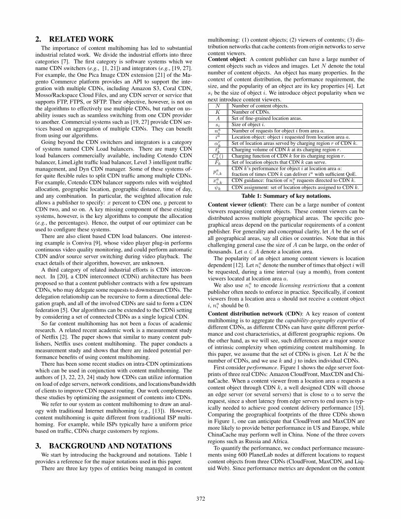
Figure 2 shows the real charging structures of two CDNs: Ama-zon CloudFront and MaxCDN. We show these two structures be-cause they are public and represent typical CDN charging struc-tures. We make three observations. First, each CDN groups thelocations of its edge servers into multiple regions and each regionmay have a different pricing model. We refer to each such re-gion as a charging region. For example, CloudFront divides into5 charging regions: US, EU, South America (SA), Japan (JP), andSingapore/Hong Kong (SHK). MaxCDN divides into 2 chargingregions: US/EU/SA, and Asia Pacific (AP). The total charge of aCDN to a content publisher is the sum of the charges at all of thecharging regions. Second, denote the total traffic originated fromthe edge servers of a CDN located at a charging region during abilling period as the charging volume of the charging region; thenthe charging function of each charging region is a nonlinear con-

cave function of the charging volume. Third, there can be largeprice diversity within a CDN as well as across CDNs. For exam-ple, CloudFront’s charge for South America for "next 100 TB" is$0.18/GB, which is 3 times that for US at the same traffic volume.

To precisely express the charging of CDNs, we let αrk be the setof location areas served by charging region r of CDN k. For view-ers from a location area a, each CDN has its own strategy to selectservers in some r to serve them. This strategy is controlled by CDNk but can be observed by content publishers [25]. For instance, inour measurements, requests from Beijing are redirected to Cloud-Front’s JP region but to MaxCDN’s US/EU/SA region. Let trk de-note the charging volume of CDN k at its charging region r, duringa billing period. Specifically, the value of trk is computed as thetotal traffic delivered during the billing period to content viewers atlocation areas who are assigned to αrk by CDN k. Then the totalcharge of CDN k to the content publisher is a sum of the charges atindividual charging regions. Let Crk() denote the charging functionof CDN k for its charging region r.

4. CONTROL FRAMEWORKWe adopt a general, practical content publishing control frame-

work shown in Figure 3. A central Optimizer computes configu-rations to direct viewer requests to CDNs. The configurations aresent to a DNS system, HTTP redirector, or a manifest-file serversystem to implement direction for specific viewer requests.

In particular, we distinguish two types of clients according totheir capabilities. This distinction affects our problem formulation.The first type is passive clients. A key characteristic of passiveclients is that they use one CDN edge server at a time. Althoughmultiple CDNs and/or multiple servers from one CDN are availablein content multihoming, such traditional clients at content viewersuse only a single CDN server to serve a particular content objectrequest [2]. For such clients, we assume that the results of con-tent multihoming optimization are implemented only by server sidemechanisms such as DNS redirection.

Specifically, suppose that content publisher cp.com uses DNS-based CDN redirection. For simplicity, say the publisher assignscontent object i URL http://obj-i.cp.com. When a clientrequests this link, a DNS query from the client or the local DNSserver of the client to resolve obj-i.cp.com can be sent to theDNS server of the content publisher, labeled CPDNS in Figure 3.By looking up the IP address of the client or the local DNS resolverof the client, CPDNS obtains the location area a. Using the outputfrom the Optimizer, CPDNS returns to the client the CNAME of achosen CDN k. As an example shown in Figure 3, CloudFront ischosen. Note in real implementations, as we will see in Section 6,URL assignment is not necessarily per-object. Alternative imple-mentations (e.g., using HTTP-based CDN redirection) are similar.

The second type is active clients. Such clients include an adap-tation algorithm (e.g., in Adobe Flash ActionScript) to utilize mul-tiple CDN servers when retrieving a single content object. In par-ticular, when the service rate of one CDN server is insufficient,an active client can use additional servers (from the same CDN orbackup CDNs) to make up the deficit. The additional CDNs/serversare provided to the adaptation algorithm through a manifest filefrom the content publisher. Such manifest files are already used bysome clients such as the Netflix clients. As shown in Figure 3, theCNAMEs of two CDNs are returned to an active client.

5. PROBLEM STATEMENTSWith the preceding background and control framework, our prob-

lems are easy to state. Note that there is much flexibility in the de-ployment of our control framework. There can be settings with onlypassive clients, or only active clients, or a hybrid. We first state the

373

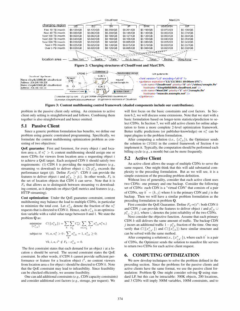
Figure 2: Charging structures of CloudFront and MaxCDN.

Figure 3: Content multihoming control framework (shaded components include our contributions).

problem in the passive client only setting. An extension to activeclient only setting is straightforward and follows. Combining themtogether is also straightforward and hence omitted.

5.1 Passive ClientSince a generic problem formulation has benefits, we define our

problem using generic constrained programming. Specifically, weformulate the content multihoming optimization problem as con-sisting of two objectives:

QoE guarantee: First and foremost, for every object i and loca-tion area a, if nai > 0, content multihoming should assign one ormore CDNs for viewers from location area a requesting object ito achieve a QoE target. Each assigned CDN k should satisfy tworequirements: (1) CDN k is providing the required features (e.g.,streaming vs download) to deliver object i; (2) pai,k exceeds theperformance target (p̄). Define Fk={ia: CDN k can provide thefeatures to deliver object i and pai,k ≥ p̄.}. In other words, Fk isthe set of location objects that CDN k can serve. Note that it isFk that allows us to distinguish between streaming vs download-ing content, as it depends on object QoE metrics and features (e.g.,HTTP-streaming).

Cost optimization: Under the QoE guarantee constraint, contentmultihoming may balance the load to multiple CDNs, in particularto minimize the total cost. Let xai,k denote the fraction of the nairequests that is directed to CDN k. Hence, each xai,k is an optimiza-tion variable with a valid value range between 0 and 1. We state theproblem Q as:

minimize{xa

i,k}

C({xai,k}) =∑

k

∑

αrk

Crk(∑

a∈αrk

∑

i

xai,knai si)

subject to ∀i, a, nai > 0 :∑

k

xai,k = 1, xai,k ≥ 0;

∀k, i, a, ia /∈ Fk : xai,k = 0.

The first constraint states that each demand for an object i at a lo-cation a should be served. The second constraint states the QoEconstraint. In other words, if CDN k cannot provide sufficient per-formance or feature for a location object ia, no content viewersfrom location area a for object i should be directed to CDN k. Notethat the QoE constraint may lead to infeasibility. Since feasibilitycan be checked efficiently, we assume feasibility.

One can add additional constraints (e.g., CDN capacity constraints)and consider additional cost factors (e.g., storage, per request). We

will first focus on the basic constraints and cost factors. In Sec-tion 6.2, we will discuss some extensions. Note that we start with abasic formulation based on longer-term statistics/prediction to se-lect CDNs. In Section 7, we will add active clients for online adap-tation to form a more complete 2-level optimization framework.Better traffic predictions (or publisher-knowledge) on nai can beinput plugins to the problem formulation.

After computing a solution (i.e., {xai,k}), the Optimizer sendsthe solution to CPDNS in the control framework of Section 4 toimplement it. Typically, the computation should be performed eachbilling cycle (e.g., a month) but can be more frequently.

5.2 Active ClientAn active client allows the usage of multiple CDNs to serve the

same request. One might think that this will add substantial com-plexity to the preceding formulation. But as we will see, it is asimple extension of the preceding problem definition.

Without loss of generality, consider that each active client usestwo CDNs: one primary and one backup. Consider the followingset of CDNs: each CDN is a "virtual CDN" that consists of a pairof CDNs, say k

′= (k, j) where k is the primary CDN and j is the

backup. Then we will have a similar problem formulation as thepreceding formulation in problem Q.

First consider the QoE Guarantee. Define Fk′={ia: both CDN kand CDN j can provide the features to deliver object i and pai,k ∪pai,j ≥ p̄.}, where ∪ denotes the joint reliability of the two CDNs.

Next consider the objective function. Assume that each primaryCDN k still delivers the same amount of traffic. The backup CDNj incurs an additional traffic 1− pai,k fraction of the time. One mayverify that C({xa

i,k′ }) and C({xai,k}) have similar structure and

can be solved with the same method.After computing a solution(i.e., {xa

i,k′ }), where each k

′is a pair

of CDNs, the Optimizer sends the solution to manifest file serversto return two CDNs for each active client request.

6. COMPUTING OPTIMIZATIONWe now develop techniques to solve the problem defined in the

preceding section. Since the problems for the passive clients andactive clients have the same format, we use the passive client for-mulation: Problem Q. One might consider solving Q using stan-dard LP, but this can be intractable: 500K objects, 200 locations,and 3 CDNs will imply 300M variables, 100M constraints, and to

374

minimize a concave function. No generic solver we know can han-dle this case, so we develop our specific algorithm.

Our strategy is to first transform the problem to a combinato-rial assignment problem in Section 6.1. Then, in Section 6.2 wedevelop a novel, efficient algorithm that computes an optimal as-signment without enumerating all of the exponentially many possi-bilities. We discuss extensions in Section 6.3.

6.1 Location Object AssignmentAt a first glance of the problem Q, one might think about us-

ing convex programming (e.g., [6]) to solve the problem. Unfortu-nately, the objective function C({xai,k}), which we target to min-imize, is a concave function. Hence, traditional, efficient convexprogramming does not apply.

On the other hand, the concavity of the objective does lead toone observation: there is a minimizer of problem Q such that eachlocation object is put into only one CDN. Precisely, we have:

LEMMA 1. There exists a minimizer of C({xai,k}) for problemQ, in which for each location object ia, there exists a CDN k∗ suchthat ia ∈ Fk∗ , and xai,k∗ = 1.

Consider one such solution, and let ψ denote the assignment (ormapping), according to the solution, from each location object ia

to its assigned single CDN k: ψ(ia) = k. Let ψk denote the set oflocation objects that are assigned to CDN k. If ∀k, ∀ia ∈ ψk wehave ia ∈ Fk, we call ψ a feasible assignment.

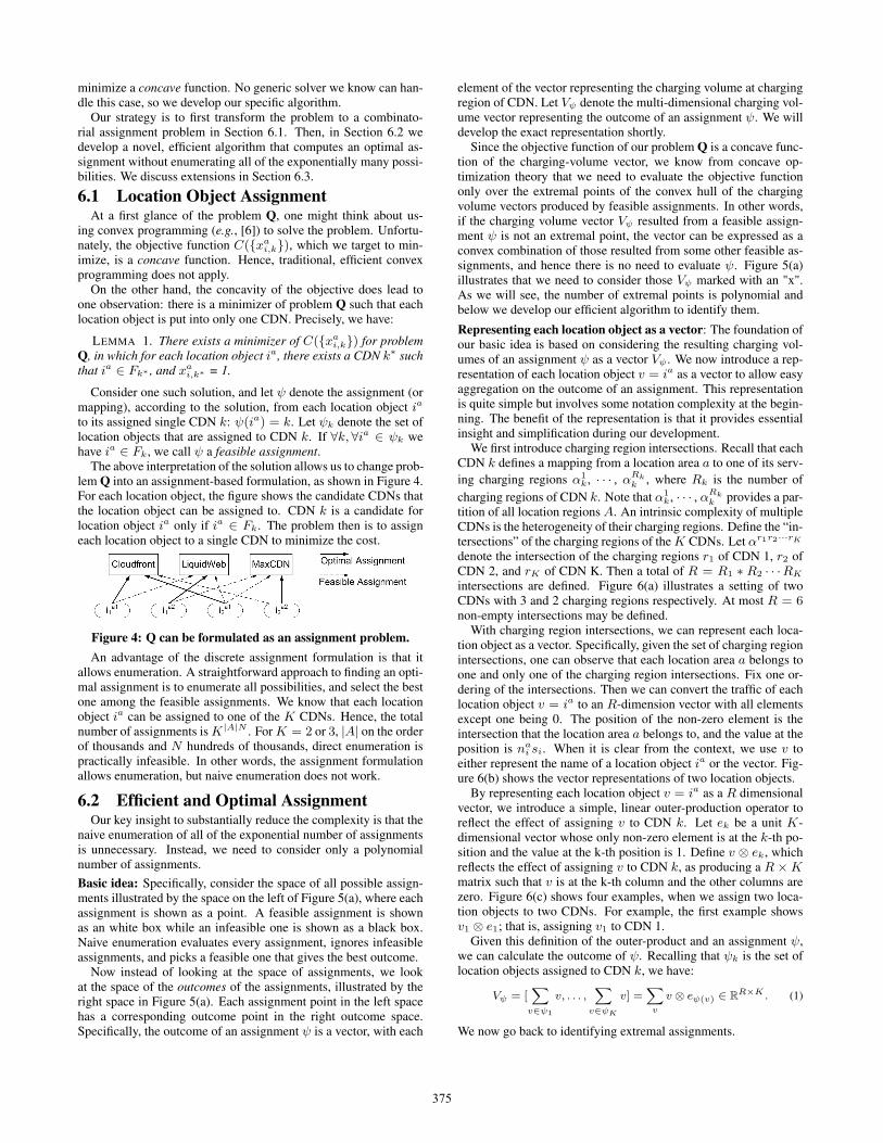
The above interpretation of the solution allows us to change prob-lem Q into an assignment-based formulation, as shown in Figure 4.For each location object, the figure shows the candidate CDNs thatthe location object can be assigned to. CDN k is a candidate forlocation object ia only if ia ∈ Fk. The problem then is to assigneach location object to a single CDN to minimize the cost.

Figure 4: Q can be formulated as an assignment problem.

An advantage of the discrete assignment formulation is that itallows enumeration. A straightforward approach to finding an opti-mal assignment is to enumerate all possibilities, and select the bestone among the feasible assignments. We know that each locationobject ia can be assigned to one of the K CDNs. Hence, the totalnumber of assignments isK|A|N . ForK = 2 or 3, |A| on the orderof thousands and N hundreds of thousands, direct enumeration ispractically infeasible. In other words, the assignment formulationallows enumeration, but naive enumeration does not work.

6.2 Efficient and Optimal AssignmentOur key insight to substantially reduce the complexity is that the

naive enumeration of all of the exponential number of assignmentsis unnecessary. Instead, we need to consider only a polynomialnumber of assignments.

Basic idea: Specifically, consider the space of all possible assign-ments illustrated by the space on the left of Figure 5(a), where eachassignment is shown as a point. A feasible assignment is shownas an white box while an infeasible one is shown as a black box.Naive enumeration evaluates every assignment, ignores infeasibleassignments, and picks a feasible one that gives the best outcome.

Now instead of looking at the space of assignments, we lookat the space of the outcomes of the assignments, illustrated by theright space in Figure 5(a). Each assignment point in the left spacehas a corresponding outcome point in the right outcome space.Specifically, the outcome of an assignment ψ is a vector, with each

element of the vector representing the charging volume at chargingregion of CDN. Let Vψ denote the multi-dimensional charging vol-ume vector representing the outcome of an assignment ψ. We willdevelop the exact representation shortly.

Since the objective function of our problem Q is a concave func-tion of the charging-volume vector, we know from concave op-timization theory that we need to evaluate the objective functiononly over the extremal points of the convex hull of the chargingvolume vectors produced by feasible assignments. In other words,if the charging volume vector Vψ resulted from a feasible assign-ment ψ is not an extremal point, the vector can be expressed as aconvex combination of those resulted from some other feasible as-signments, and hence there is no need to evaluate ψ. Figure 5(a)illustrates that we need to consider those Vψ marked with an "x".As we will see, the number of extremal points is polynomial andbelow we develop our efficient algorithm to identify them.

Representing each location object as a vector: The foundation ofour basic idea is based on considering the resulting charging vol-umes of an assignment ψ as a vector Vψ . We now introduce a rep-resentation of each location object v = ia as a vector to allow easyaggregation on the outcome of an assignment. This representationis quite simple but involves some notation complexity at the begin-ning. The benefit of the representation is that it provides essentialinsight and simplification during our development.

We first introduce charging region intersections. Recall that eachCDN k defines a mapping from a location area a to one of its serv-ing charging regions α1

k, · · · , αRkk , where Rk is the number of

charging regions of CDN k. Note that α1k, · · · , αRk

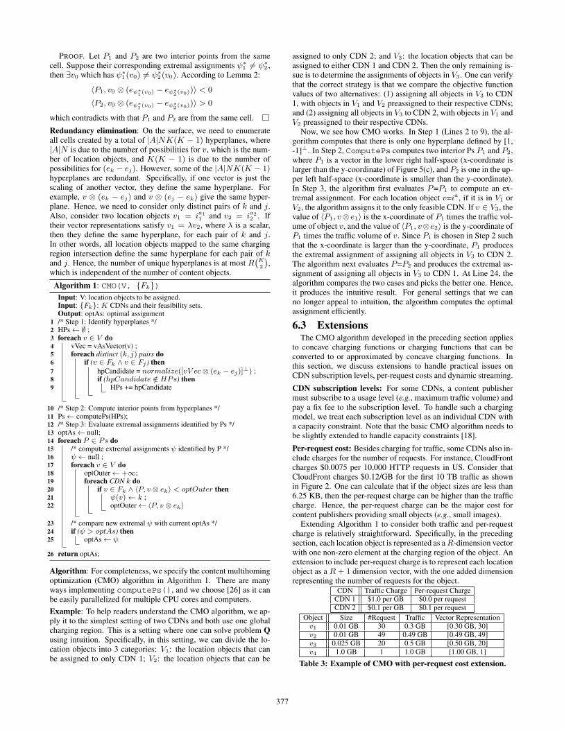
k provides a par-tition of all location regions A. An intrinsic complexity of multipleCDNs is the heterogeneity of their charging regions. Define the “in-tersections” of the charging regions of theK CDNs. Let αr1r2···rKdenote the intersection of the charging regions r1 of CDN 1, r2 ofCDN 2, and rK of CDN K. Then a total of R = R1 ∗ R2 · · ·RKintersections are defined. Figure 6(a) illustrates a setting of twoCDNs with 3 and 2 charging regions respectively. At most R = 6non-empty intersections may be defined.

With charging region intersections, we can represent each loca-tion object as a vector. Specifically, given the set of charging regionintersections, one can observe that each location area a belongs toone and only one of the charging region intersections. Fix one or-dering of the intersections. Then we can convert the traffic of eachlocation object v = ia to an R-dimension vector with all elementsexcept one being 0. The position of the non-zero element is theintersection that the location area a belongs to, and the value at theposition is nai si. When it is clear from the context, we use v toeither represent the name of a location object ia or the vector. Fig-ure 6(b) shows the vector representations of two location objects.

By representing each location object v = ia as a R dimensionalvector, we introduce a simple, linear outer-production operator toreflect the effect of assigning v to CDN k. Let ek be a unit K-dimensional vector whose only non-zero element is at the k-th po-sition and the value at the k-th position is 1. Define v ⊗ ek, whichreflects the effect of assigning v to CDN k, as producing a R ×Kmatrix such that v is at the k-th column and the other columns arezero. Figure 6(c) shows four examples, when we assign two loca-tion objects to two CDNs. For example, the first example showsv1 ⊗ e1; that is, assigning v1 to CDN 1.

Given this definition of the outer-product and an assignment ψ,we can calculate the outcome of ψ. Recalling that ψk is the set oflocation objects assigned to CDN k, we have:

Vψ = [∑

v∈ψ1

v, . . . ,∑

v∈ψK

v] =∑

v

v ⊗ eψ(v) ∈ RR×K . (1)

We now go back to identifying extremal assignments.

375

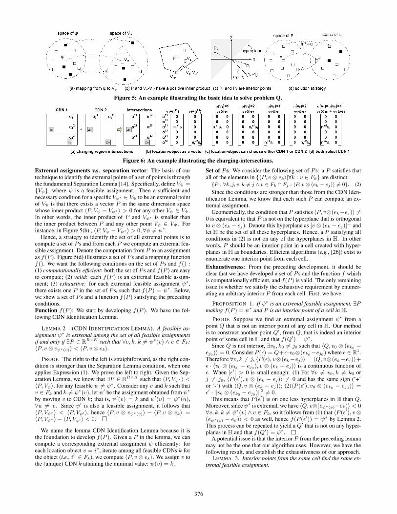
Figure 5: An example illustrating the basic idea to solve problem Q.

Figure 6: An example illustrating the charging-intersections.

Extremal assignments v.s. separation vector: The basis of ourtechnique to identify the extremal points of a set of points is throughthe fundamental Separation Lemma [14]. Specifically, define VΨ ={Vψ}, where ψ is a feasible assignment. Then a sufficient andnecessary condition for a specific Vψ∗ ∈ VΨ to be an extremal pointof VΨ is that there exists a vector P in the same dimension spacewhose inner product 〈P, Vψ − Vψ∗〉 > 0 for any other Vψ ∈ VΨ.In other words, the inner product of P and Vψ∗ is smaller thanthe inner product between P and any other point Vψ ∈ VΨ. Forinstance, in Figure 5(b) , 〈P, Vψ − Vψ∗〉 > 0, ∀ψ = ψ∗.

Hence, a strategy to identify the set of all extremal points is tocompute a set of P s and from each P we compute an extremal fea-sible assignment. Denote the computation from P to an assignmentas f(P ). Figure 5(d) illustrates a set of P s and a mapping functionf(). We want the following conditions on the set of P s and f() :(1) computationally efficient: both the set of P s and f(P ) are easyto compute; (2) valid: each f(P ) is an extremal feasible assign-ment; (3) exhaustive: for each extremal feasible assignment ψ∗,there exists one P in the set of P s, such that f(P ) = ψ∗. Below,we show a set of P s and a function f(P ) satisfying the precedingconditions.Function f(P ): We start by developing f(P ). We have the fol-lowing CDN Identification Lemma.

LEMMA 2 (CDN IDENTIFICATION LEMMA). A feasible as-signment ψ∗ is extremal among the set of all feasible assignmentsif and only if ∃P ∈ R

R×K such that ∀v, k, k = ψ∗(v) ∧ v ∈ Fk:〈P, v ⊗ eψ∗(v)〉 < 〈P, v ⊗ ek〉.

PROOF. The right to the left is straightforward, as the right con-dition is stronger than the Separation Lemma condition, when oneapplies Expression (1). We prove the left to right. Given the Sep-aration Lemma, we know that ∃P ∈ R

R×K such that 〈P, Vψ∗〉 <〈P, Vψ〉, for any feasible ψ = ψ∗. Consider any v and k such thatv ∈ Fk and k = ψ∗(v), let ψ′ be the assignment obtained from ψ∗

by moving v to CDN k; that is, ψ′(v) = k and ψ′(u) = ψ∗(u),∀u = v. Since ψ′ is also a feasible assignment, it follows that〈P, Vψ∗〉 < 〈P, Vψ′〉, hence 〈P, v ⊗ eψ∗(v)〉 − 〈P, v ⊗ ek〉 =〈P, Vψ∗〉 − 〈P, Vψ′〉 < 0.

We name the lemma CDN Identification Lemma because it isthe foundation to develop f(P ). Given a P in the lemma, we cancompute a corresponding extremal assignment ψ efficiently: foreach location object v = ia, iterate among all feasible CDNs k forthe object (i.e., ia ∈ Fk), we compute 〈P, v ⊗ ek〉. We assign v tothe (unique) CDN k attaining the minimal value: ψ(v) = k.

Set of P s: We consider the following set of P s: a P satisfies thatall of the elements in {〈P, v ⊗ ek〉|∀k : v ∈ Fk} are distinct:{P : ∀k, j, v, k �= j ∧ v ∈ Fk ∩ Fj : 〈P, v ⊗ (ek − ej)〉 �= 0}. (2)

Since the conditions are stronger than those from the CDN Iden-tification Lemma, we know that each such P can compute an ex-tremal assignment.

Geometrically, the condition that P satisfies 〈P, v⊗(ek−ej)〉 =0 is equivalent to that P is not on the hyperplane that is orthogonalto v ⊗ (ek − ej). Denote this hyperplane as [v ⊗ (ek − ej)]

⊥ andlet H be the set of all these hyperplanes. Hence, a P satisfying allconditions in (2) is not on any of the hyperplanes in H. In otherwords, P should be an interior point in a cell created with hyper-planes in H as boundaries. Efficient algorithms (e.g., [26]) exist toenumerate one interior point from each cell.

Exhaustiveness: From the preceding development, it should beclear that we have developed a set of P s and the function f whichis computationally efficient, and f(P ) is valid. The only remainingissue is whether we satisfy the exhaustive requirement by enumer-ating an arbitrary interior P from each cell. First, we have

PROPOSITION 1. If ψ∗ is an extremal feasible assignment, ∃Pmaking f(P ) = ψ∗ and P is an interior point of a cell in H.

PROOF. Suppose we find an extremal assignment ψ∗ from apoint Q that is not an interior point of any cell in H. Our methodis to construct another point Q′, from Q, that is indeed an interiorpoint of some cell in H and that f(Q′) = ψ∗.

Since Q is not interior, ∃v0, k0 = j0 such that 〈Q, v0 ⊗ (ek0 −ej0)〉 = 0. Consider P (ε) = Q+ε·v0⊗(ek0−ej0) where ε ∈ R

1.Therefore ∀v, k = j, 〈P (ε), v⊗(ek−ej)〉 = 〈Q, v⊗(ek−ej)〉+ε · 〈v0 ⊗ (ek0 − ej0), v ⊗ (ek − ej)〉 is a continuous function ofε. When |ε′| > 0 is small enough: (1) For ∀v = v0, k = k0 orj = j0, 〈P (ε′), v ⊗ (ek − ej)〉 = 0 and has the same sign (’+’or ’-’) with 〈Q, v ⊗ (ek − ej)〉; (2)〈P (ε′), v0 ⊗ (ek0 − ej0)〉 =ε′ · ‖v0 ⊗ (ek0 − ej0)‖2 = 0.

This means that P (ε′) is on one less hyperplanes in H than Q.Moreover, sinceψ∗ is extremal, we have 〈Q, v⊗(eψ∗(v)−ek)〉 < 0∀v, k, k = ψ∗(v)∧ v ∈ Fk, so it follows from (1) that 〈P (ε′), v⊗(eψ∗(v) − ek)〉 < 0 as well, hence f(P (ε′)) = ψ∗ by Lemma 2.This process can be repeated to yield a Q′ that is not on any hyper-planes in H and that f(Q′) = ψ∗.

A potential issue is that the interior P from the preceding lemmamay not be the one that our algorithm uses. However, we have thefollowing result, and establish the exhaustiveness of our approach.

LEMMA 3. Interior points from the same cell find the same ex-tremal feasible assignment.

376

PROOF. Let P1 and P2 are two interior points from the samecell. Suppose their corresponding extremal assignments ψ∗

1 = ψ∗2 ,

then ∃v0 which has ψ∗1(v0) = ψ∗

2(v0). According to Lemma 2:

〈P1, v0 ⊗ (eψ∗1 (v0) − eψ∗

2 (v0))〉 < 0

〈P2, v0 ⊗ (eψ∗1 (v0) − eψ∗

2 (v0))〉 > 0

which contradicts with that P1 and P2 are from the same cell.

Redundancy elimination: On the surface, we need to enumerateall cells created by a total of |A|NK(K − 1) hyperplanes, where|A|N is due to the number of possibilities for v, which is the num-ber of location objects, and K(K − 1) is due to the number ofpossibilities for (ek − ej). However, some of the |A|NK(K − 1)hyperplanes are redundant. Specifically, if one vector is just thescaling of another vector, they define the same hyperplane. Forexample, v ⊗ (ek − ej) and v ⊗ (ej − ek) give the same hyper-plane. Hence, we need to consider only distinct pairs of k and j.Also, consider two location objects v1 = ia11 and v2 = ia22 . Iftheir vector representations satisfy v1 = λv2, where λ is a scalar,then they define the same hyperplane, for each pair of k and j.In other words, all location objects mapped to the same chargingregion intersection define the same hyperplane for each pair of kand j. Hence, the number of unique hyperplanes is at most R

(K2

),

which is independent of the number of content objects.

Algorithm 1: CMO(V, {Fk})Input: V: location objects to be assigned.Input: {Fk}: K CDNs and their feasibility sets.Output: optAs: optimal assignment/* Step 1: Identify hyperplanes */1HPs← ∅ ;2foreach v ∈ V do3

vVec = vAsVector(v) ;4foreach distinct (k, j) pairs do5

if (v ∈ Fk ∧ v ∈ Fj ) then6hpCandidate = normalize([vV ec⊗ (ek − ej)]⊥) ;7if (hpCandidate /∈ HPs) then8

HPs += hpCandidate9

/* Step 2: Compute interior points from hyperplanes */10Ps← computePs(HPs);11/* Step 3: Evaluate extremal assignments identified by Ps */12optAs← null;13foreach P ∈ Ps do14

/* compute extremal assignments ψ identified by P */15ψ← null ;16foreach v ∈ V do17

optOuter← +∞;18foreach CDN k do19

if v ∈ Fk ∧ 〈P, v ⊗ ek〉 < optOuter then20ψ(v)← k ;21optOuter← 〈P, v ⊗ ek〉22

/* compare new extremal ψ with current optAs */23if (ψ > optAs) then24

optAs← ψ25

return optAs;26

Algorithm: For completeness, we specify the content multihomingoptimization (CMO) algorithm in Algorithm 1. There are manyways implementing computePs(), and we choose [26] as it canbe easily parallelized for multiple CPU cores and computers.

Example: To help readers understand the CMO algorithm, we ap-ply it to the simplest setting of two CDNs and both use one globalcharging region. This is a setting where one can solve problem Qusing intuition. Specifically, in this setting, we can divide the lo-cation objects into 3 categories: V1: the location objects that canbe assigned to only CDN 1; V2: the location objects that can be

assigned to only CDN 2; and V3: the location objects that can beassigned to either CDN 1 and CDN 2. Then the only remaining is-sue is to determine the assignments of objects in V3. One can verifythat the correct strategy is that we compare the objective functionvalues of two alternatives: (1) assigning all objects in V3 to CDN1, with objects in V1 and V2 preassigned to their respective CDNs;and (2) assigning all objects in V3 to CDN 2, with objects in V1 andV2 preassigned to their respective CDNs.

Now, we see how CMO works. In Step 1 (Lines 2 to 9), the al-gorithm computes that there is only one hyperplane defined by [1,-1]⊥. In Step 2, ComputePs computes two interior Ps P1 and P2,where P1 is a vector in the lower right half-space (x-coordinate islarger than the y-coordinate) of Figure 5(c), and P2 is one in the up-per left half-space (x-coordinate is smaller than the y-coordinate).In Step 3, the algorithm first evaluates P=P1 to compute an ex-tremal assignment. For each location object v=ia, if it is in V1 orV2, the algorithm assigns it to the only feasible CDN. If v ∈ V3, thevalue of 〈P1, v⊗ e1〉 is the x-coordinate of P1 times the traffic vol-ume of object v, and the value of 〈P1, v⊗e2〉 is the y-coordinate ofP1 times the traffic volume of v. Since P1 is chosen in Step 2 suchthat the x-coordinate is larger than the y-coordinate, P1 producesthe extremal assignment of assigning all objects in V3 to CDN 2.The algorithm next evaluates P=P2 and produces the extremal as-signment of assigning all objects in V3 to CDN 1. At Line 24, thealgorithm compares the two cases and picks the better one. Hence,it produces the intuitive result. For general settings that we canno longer appeal to intuition, the algorithm computes the optimalassignment efficiently.

6.3 ExtensionsThe CMO algorithm developed in the preceding section applies

to concave charging functions or charging functions that can beconverted to or approximated by concave charging functions. Inthis section, we discuss extensions to handle practical issues onCDN subscription levels, per-request costs and dynamic streaming.

CDN subscription levels: For some CDNs, a content publishermust subscribe to a usage level (e.g., maximum traffic volume) andpay a fix fee to the subscription level. To handle such a chargingmodel, we treat each subscription level as an individual CDN witha capacity constraint. Note that the basic CMO algorithm needs tobe slightly extended to handle capacity constraints [18].

Per-request cost: Besides charging for traffic, some CDNs also in-clude charges for the number of requests. For instance, CloudFrontcharges $0.0075 per 10,000 HTTP requests in US. Consider thatCloudFront charges $0.12/GB for the first 10 TB traffic as shownin Figure 2. One can calculate that if the object sizes are less than6.25 KB, then the per-request charge can be higher than the trafficcharge. Hence, the per-request charge can be the major cost forcontent publishers providing small objects (e.g., small images).

Extending Algorithm 1 to consider both traffic and per-requestcharge is relatively straightforward. Specifically, in the precedingsection, each location object is represented as aR-dimension vectorwith one non-zero element at the charging region of the object. Anextension to include per-request charge is to represent each locationobject as a R+ 1 dimension vector, with the one added dimensionrepresenting the number of requests for the object.

CDN Traffic Charge Per-request ChargeCDN 1 $1.0 per GB $0.0 per requestCDN 2 $0.1 per GB $0.1 per request

Object Size #Request Traffic Vector Representationv1 0.01 GB 30 0.3 GB [0.30 GB, 30]v2 0.01 GB 49 0.49 GB [0.49 GB, 49]v3 0.025 GB 20 0.5 GB [0.50 GB, 20]v4 1.0 GB 1 1.0 GB [1.00 GB, 1]

Table 3: Example of CMO with per-request cost extension.

377

We demonstrate the extension using an example setting (Table 3):4 objects, 2 CDNs with one charging region (i.e., R = 1):

• First the 4 objects are represented as 4 2D vectors (see Table 3).

• Lines 3 to 9 construct four corresponding hyperplanes: h1 = [0.3,-0.3,30,-30]⊥, h2 = [0.49,-0.49,49,-49]⊥, h3 = [0.5,-0.5,20,-20]⊥, h4 =[1,-1,1,-1]⊥. After normalization and de-duplication (Lines 7, 8),only three are left: [1,-1,100,-100]⊥, [1,-1,40,-40]⊥, [1,-1,1,-1]⊥;i.e., first two are redundant and only 1 is needed.

• Line 11 finds 6 interior points: P1 = [1,0,1,0], P2 = [-1,0,-1,0], P3

= [70,0,-1,0], P4 = [-70,0,1,0] , P5 = [20,0,-1,0], P6 = [-20,0,1,0].

• Lines 14 to 22 find 6 extremal object assignments (ψ :={CDN1objects}{CDN2 objects}): ψ1 = {}{v1, v2, v3, v4}, ψ2 = {v1, v2, v3,v4}{}, ψ3 = {v1, v2} {v3, v4}, ψ4 = {v3, v4} {v1, v2}, ψ5 = {v1, v2,v3} {v4}, ψ6 = {v4} {v1, v2, v3}.

• Lines 23 to 25 enumerate the costs of the 6 extremal object as-signments, and identify optimal assignment ψ5. As a compari-son, simple enumerations need to consider 16 assignment possi-bilities (4 objects each with 2 possible assignments).

Multiple streaming rates: A content publisher can encode thesame video object at multiple rates, and a client can switch amongthe encoding rates dynamically online. To extend CMO for this set-ting, one can consider each video at each encoding rate as an inde-pendent object and then derive the number of requests to each suchobject. Specifically, suppose a total of nai requests for video i fromlocation area a when there is no multi-rate. Consider two encodingrates, say 1x and 2x. Then according to client access bandwidthdistribution at location area a and the publisher dynamic streamingalgorithm, one can derive nai1 and nai2 for the two encoding ratesfrom nai [18].

7. ACTIVE CLIENTSAn active client is provided with a list of CDNs to use when

requesting a single content object. The list may come from theresult of our optimization algorithm in the preceding section or an-other source of guidance. Even though our optimization algorithmconsiders performance constraints, the filtering is based on long-term statistics. Hence, the objective of the active client is to adaptto specific real-time CDN performance dynamics, in particular, toimprove QoE during CDN server failures.

7.1 Adaptation Problem StatementAn active client receives guidance in the format of a list of CDNs

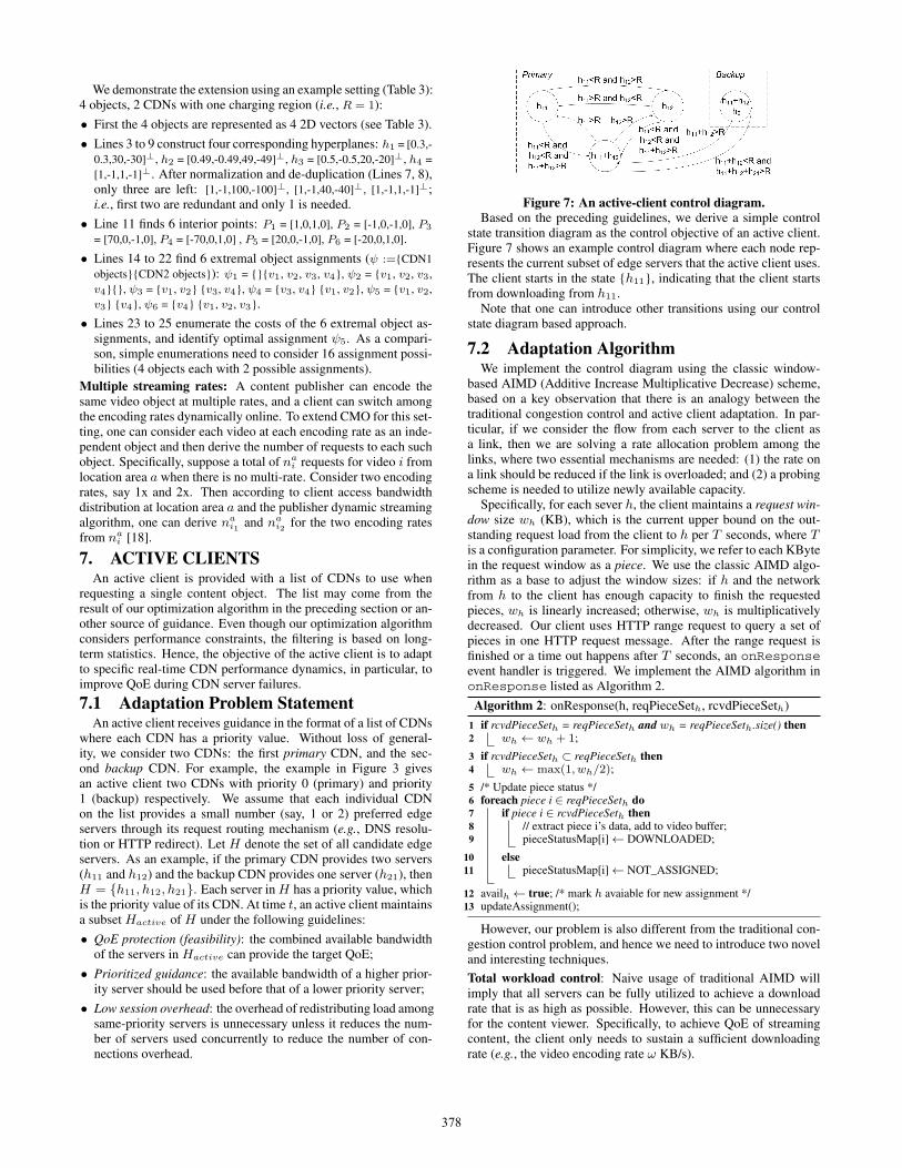
where each CDN has a priority value. Without loss of general-ity, we consider two CDNs: the first primary CDN, and the sec-ond backup CDN. For example, the example in Figure 3 givesan active client two CDNs with priority 0 (primary) and priority1 (backup) respectively. We assume that each individual CDNon the list provides a small number (say, 1 or 2) preferred edgeservers through its request routing mechanism (e.g., DNS resolu-tion or HTTP redirect). Let H denote the set of all candidate edgeservers. As an example, if the primary CDN provides two servers(h11 and h12) and the backup CDN provides one server (h21), thenH = {h11, h12, h21}. Each server inH has a priority value, whichis the priority value of its CDN. At time t, an active client maintainsa subset Hactive of H under the following guidelines:

• QoE protection (feasibility): the combined available bandwidthof the servers in Hactive can provide the target QoE;

• Prioritized guidance: the available bandwidth of a higher prior-ity server should be used before that of a lower priority server;

• Low session overhead: the overhead of redistributing load amongsame-priority servers is unnecessary unless it reduces the num-ber of servers used concurrently to reduce the number of con-nections overhead.

Figure 7: An active-client control diagram.Based on the preceding guidelines, we derive a simple control

state transition diagram as the control objective of an active client.Figure 7 shows an example control diagram where each node rep-resents the current subset of edge servers that the active client uses.The client starts in the state {h11}, indicating that the client startsfrom downloading from h11.

Note that one can introduce other transitions using our controlstate diagram based approach.

7.2 Adaptation AlgorithmWe implement the control diagram using the classic window-

based AIMD (Additive Increase Multiplicative Decrease) scheme,based on a key observation that there is an analogy between thetraditional congestion control and active client adaptation. In par-ticular, if we consider the flow from each server to the client asa link, then we are solving a rate allocation problem among thelinks, where two essential mechanisms are needed: (1) the rate ona link should be reduced if the link is overloaded; and (2) a probingscheme is needed to utilize newly available capacity.

Specifically, for each sever h, the client maintains a request win-dow size wh (KB), which is the current upper bound on the out-standing request load from the client to h per T seconds, where Tis a configuration parameter. For simplicity, we refer to each KBytein the request window as a piece. We use the classic AIMD algo-rithm as a base to adjust the window sizes: if h and the networkfrom h to the client has enough capacity to finish the requestedpieces, wh is linearly increased; otherwise, wh is multiplicativelydecreased. Our client uses HTTP range request to query a set ofpieces in one HTTP request message. After the range request isfinished or a time out happens after T seconds, an onResponseevent handler is triggered. We implement the AIMD algorithm inonResponse listed as Algorithm 2.

Algorithm 2: onResponse(h, reqPieceSeth, rcvdPieceSeth)

if rcvdPieceSeth = reqPieceSeth and wh = reqPieceSeth.size() then1wh ← wh + 1;2

if rcvdPieceSeth ⊂ reqPieceSeth then3wh ← max(1, wh/2);4

/* Update piece status */5foreach piece i ∈ reqPieceSeth do6

if piece i ∈ rcvdPieceSeth then7// extract piece i’s data, add to video buffer;8pieceStatusMap[i]← DOWNLOADED;9

else10pieceStatusMap[i]← NOT_ASSIGNED;11

availh← true; /* mark h avaiable for new assignment */12updateAssignment();13

However, our problem is also different from the traditional con-gestion control problem, and hence we need to introduce two noveland interesting techniques.

Total workload control: Naive usage of traditional AIMD willimply that all servers can be fully utilized to achieve a downloadrate that is as high as possible. However, this can be unnecessaryfor the content viewer. Specifically, to achieve QoE of streamingcontent, the client only needs to sustain a sufficient downloadingrate (e.g., the video encoding rate ω KB/s).

378

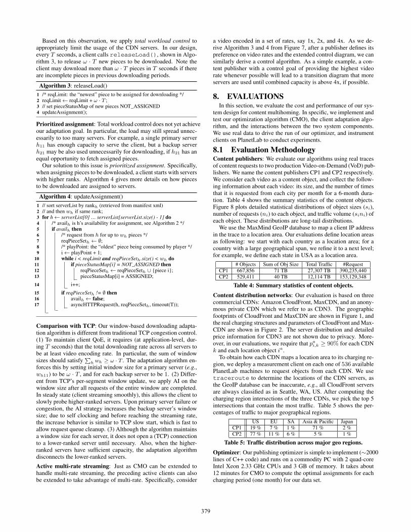
Based on this observation, we apply total workload control toappropriately limit the usage of the CDN servers. In our design,every T seconds, a client calls releaseLoad(), shown in Algo-rithm 3, to release ω · T new pieces to be downloaded. Note theclient may download more than ω · T pieces in T seconds if thereare incomplete pieces in previous downloading periods.

Algorithm 3: releaseLoad()

/* reqLimit: the “newest” piece to be assigned for downloading */1reqLimit← reqLimit + ω · T ;2// set pieceStatusMap of new pieces NOT_ASSIGNED3updateAssignment();4

Prioritized assignment: Total workload control does not yet achieveour adaptation goal. In particular, the load may still spread unnec-essarily to too many servers. For example, a single primary serverh11 has enough capacity to serve the client, but a backup serverh21 may be also used unnecessarily for downloading, if h21 has anequal opportunity to fetch assigned pieces.

Our solution to this issue is prioritized assignment. Specifically,when assigning pieces to be downloaded, a client starts with serverswith higher ranks. Algorithm 4 gives more details on how piecesto be downloaded are assigned to servers.

Algorithm 4: updateAssignment()

// sort serverList by rankh (retrieved from manifest xml)1// and then wh if same rank;2for h← serverList[0] ... serverList[serverList.size() - 1] do3

/* availh is h’s availability for assignment, see Algorithm 2 */4if availh then5

/* request from h for up to wh pieces */6reqPieceSeth← ∅;7/* playPoint: the “oldest” piece being consumed by player */8i← playPoint + 1;9while i < reqLimit and reqPieceSeth.size() < wh do10

if pieceStatusMap[i] = NOT_ASSIGNED then11reqPieceSeth← reqPieceSeth ∪ {piece i};12pieceStatusMap[i] = ASSIGNED;13

i++;14

if reqPieceSeth != ∅ then15availh← false;16asyncHTTPRequest(h, reqPieceSeth, timeout(T));17

Comparison with TCP: Our window-based downloading adapta-tion algorithm is different from traditional TCP congestion control.(1) To maintain client QoE, it requires (at application-level, dur-ing T seconds) that the total downloading rate across all servers tobe at least video encoding rate. In particular, the sum of windowsizes should satisfy

∑h wh ≥ ω · T . The adaptation algorithm en-

forces this by setting initial window size for a primary server (e.g.,wh11) to be ω · T , and for each backup server to be 1. (2) Differ-ent from TCP’s per-segment window update, we apply AI on thewindow size after all requests of the entire window are completed.In steady state (client streaming smoothly), this allows the client toslowly probe higher-ranked servers. Upon primary server failure orcongestion, the AI strategy increases the backup server’s windowsize; due to self clocking and before reaching the streaming rate,the increase behavior is similar to TCP slow start, which is fast toallow request queue cleanup. (3) Although the algorithm maintainsa window size for each server, it does not open a (TCP) connectionto a lower-ranked server until necessary. Also, when the higher-ranked servers have sufficient capacity, the adaptation algorithmdisconnects the lower-ranked servers.

Active multi-rate streaming: Just as CMO can be extended tohandle multi-rate streaming, the preceding active clients can alsobe extended to take advantage of multi-rate. Specifically, consider

a video encoded in a set of rates, say 1x, 2x, and 4x. As we de-rive Algorithm 3 and 4 from Figure 7, after a publisher defines itspreference on video rates and the extended control diagram, we cansimilarly derive a control algorithm. As a simple example, a con-tent publisher with a control goal of providing the highest videorate whenever possible will lead to a transition diagram that moreservers are used until combined capacity is above 4x, if possible.

8. EVALUATIONSIn this section, we evaluate the cost and performance of our sys-

tem design for content multihoming. In specific, we implement andtest our optimization algorithm (CMO), the client adaptation algo-rithm, and the interactions between the two system components.We use real data to drive the run of our optimizer, and instrumentclients on PlanetLab to conduct experiments.

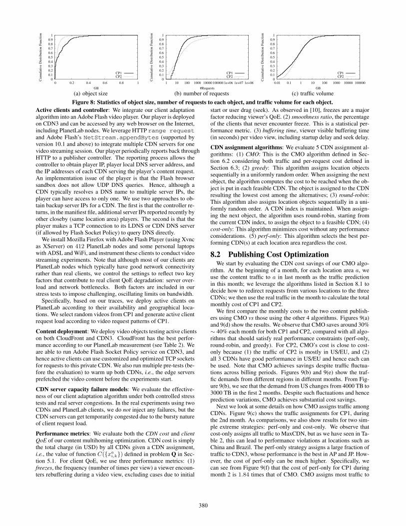
8.1 Evaluation MethodologyContent publishers: We evaluate our algorithms using real tracesof content requests to two production Video-on-Demand (VoD) pub-lishers. We name the content publishers CP1 and CP2 respectively.We consider each video as a content object, and collect the follow-ing information about each video: its size, and the number of timesthat it is requested from each city per month for a 6-month dura-tion. Table 4 shows the summary statistics of the content objects.Figure 8 plots detailed statistical distributions of object sizes (si),number of requests (ni) to each object, and traffic volume (sini) ofeach object. These distributions are long-tail distributions.

We use the MaxMind GeoIP database to map a client IP addressin the trace to a location area. Our evaluations define location areasas following: we start with each country as a location area; for acountry with a large geographical span, we refine it to a next level;for example, we define each state in USA as a location area.

# Objects Sum of Obj Size Total Traffic #RequestCP1 667,856 71 TB 27,307 TB 390,235,440CP2 529,411 40 TB 12,114 TB 153,129,348

Table 4: Summary statistics of content objects.

Content distribution networks: Our evaluation is based on threecommercial CDNs: Amazon CloudFront, MaxCDN, and an anony-mous private CDN which we refer to as CDN3. The geographicfootprints of CloudFront and MaxCDN are shown in Figure 1, andthe real charging structures and parameters of CloudFront and Max-CDN are shown in Figure 2. The server distribution and detailedprice information for CDN3 are not shown due to privacy. More-over, in our evaluations, we require that pai,k ≥ 90% for each CDNk and each location object ia.

To obtain how each CDN maps a location area to its charging re-gion, we deploy a measurement client on each one of 536 availablePlanetLab machines to request objects from each CDN. We usetraceroute to determine the locations of the CDN servers, asthe GeoIP database can be inaccurate, e.g., all CloudFront serversare always classified as in Seattle, WA, US. After computing thecharging region intersections of the three CDNs, we pick the top 5intersections that contain the most traffic. Table 5 shows the per-centages of traffic to major geographical regions.

US EU SA Asia & Pacific JapanCP1 19 % 7 % 1 % 71 % 2 %CP2 77 % 11 % 6 % 5 % 1 %

Table 5: Traffic distribution across major geo regions.

Optimizer: Our publishing optimizer is simple to implement (∼2000lines of C++ code) and runs on a commodity PC with 2 quad-coreIntel Xeon 2.33 GHz CPUs and 3 GB of memory. It takes about12 minutes for CMO to compute the optimal assignments for eachcharging period (one month) for our data set.

379

0 0.1 0.2 0.3 0.4 0.5 0.6 0.7 0.8 0.9

1

0 0.2 0.4 0.6 0.8 1

Cum

ulat

ive

Dis

trib

utio

n Fu

nctio

n

GB

CP1CP2

(a) object size

0 0.1 0.2 0.3 0.4 0.5 0.6 0.7 0.8 0.9

1

1 10 100 1000 10000 100000 1e+06 1e+07 1e+08

Cum

ulat

ive

Dis

trib

utio

n Fu

nctio

n

#Requests

CP1CP2

(b) number of requests

0 0.1 0.2 0.3 0.4 0.5 0.6 0.7 0.8 0.9

1

0.01 0.1 1 10 100 1000 10000 100000

Cum

ulat

ive

Dis

trib

utio

n Fu

nctio

n

GB

CP1CP2

(c) traffic volume

Figure 8: Statistics of object size, number of requests to each object, and traffic volume for each object.Active clients and controller: We integrate our client adaptationalgorithm into an Adobe Flash video player. Our player is deployedon CDN3 and can be accessed by any web browser on the Internet,including PlanetLab nodes. We leverage HTTP range requestand Adobe Flash’s NetStream.appendBytes (supported byversion 10.1 and above) to integrate multiple CDN servers for onevideo streaming session. Our player periodically reports back throughHTTP to a publisher controller. The reporting process allows thecontroller to obtain player IP, player local DNS server address, andthe IP addresses of each CDN serving the player’s content request.An implementation issue of the player is that the Flash browsersandbox does not allow UDP DNS queries. Hence, although aCDN typically resolves a DNS name to multiple server IPs, theplayer can have access to only one. We use two approaches to ob-tain backup server IPs for a CDN. The first is that the controller re-turns, in the manifiest file, additional server IPs reported recently byother closeby (same location area) players. The second is that theplayer makes a TCP connection to its LDNS or CDN DNS server(if allowed by Flash Socket Policy) to query DNS directly.

We install Mozilla Firefox with Adobe Flash Player (using Xvncas XServer) on 412 PlanetLab nodes and some personal laptopswith ADSL and WiFi, and instrument these clients to conduct videostreaming experiments. Note that although most of our clients arePlanetLab nodes which typically have good network connectivityrather than real clients, we control the settings to reflect two keyfactors that contribute to real client QoE degradation: server over-load and network bottlenecks. Both factors are included in ourstress tests to impose challenging, oscillating limits on bandwidth.

Specifically, based on our traces, we deploy active clients onPlanetLab according to their availability and geographical loca-tions. We select random videos from CP1 and generate active clientrequest load according to video request patterns of CP1.

Content deployment: We deploy video objects testing active clientson both CloudFront and CDN3. CloudFront has the best perfor-mance according to our PlanetLab measurement (see Table 2). Weare able to run Adobe Flash Socket Policy service on CDN3, andhence active clients can use customized and optimized TCP socketsfor requests to this private CDN. We also run multiple pre-tests (be-fore the evaluation) to warm up both CDNs, i.e., the edge serversprefetched the video content before the experiments start.

CDN server capacity failure models: We evaluate the effective-ness of our client adaptation algorithm under both controlled stresstests and real server congestions. In the real experiments using twoCDNs and PlanetLab clients, we do not inject any failures, but theCDN servers can get temporarily congested due to the bursty natureof client request load.

Performance metrics: We evaluate both the CDN cost and clientQoE of our content multihoming optimization. CDN cost is simplythe total charge (in USD) by all CDNs given a CDN assignment,i.e., the value of function C({xai,k}) defined in problem Q in Sec-tion 5.1. For client QoE, we use three performance metrics: (1)freezes, the frequency (number of times per view) a viewer encoun-ters rebuffering during a video view, excluding cases due to initial

start or user drag (seek). As observed in [10], freezes are a majorfactor reducing viewer’s QoE. (2) smoothness ratio, the percentageof the clients that never encounter freeze. This is a statistical per-formance metric. (3) buffering time, viewer visible buffering time(in seconds) per video view, including startup delay and seek delay.

CDN assignment algorithms: We evaluate 5 CDN assignment al-gorithms: (1) CMO: This is the CMO algorithm defined in Sec-tion 6.2 considering both traffic and per-request cost defined inSection 6.3; (2) greedy: This algorithm assigns location objectssequentially in a uniformly random order. When assigning the nextobject, the algorithm computes the cost to be reached when the ob-ject is put in each feasible CDN. The object is assigned to the CDNresulting the lowest cost among the alternatives; (3) round-robin:This algorithm also assigns location objects sequentially in a uni-formly random order. A CDN index is maintained. When assign-ing the next object, the algorithm uses round-robin, starting fromthe current CDN index, to assign the object to a feasible CDN; (4)cost-only: This algorithm minimizes cost without any performanceconsiderations. (5) perf-only: This algorithm selects the best per-forming CDN(s) at each location area regardless the cost.

8.2 Publishing Cost OptimizationWe start by evaluating the CDN cost savings of our CMO algo-

rithm. At the beginning of a month, for each location area a, weuse the content traffic to a in last month as the traffic predictionin this month; we leverage the algorithms listed in Section 8.1 todecide how to redirect requests from various locations to the threeCDNs; we then use the real traffic in the month to calculate the totalmonthly cost of CP1 and CP2.

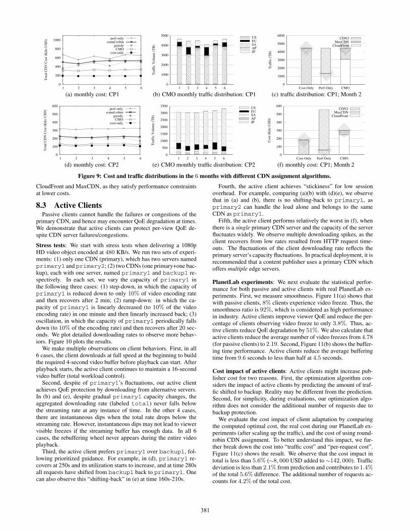
We first compare the monthly costs to the two content publish-ers using CMO vs those using the other 4 algorithms. Figures 9(a)and 9(d) show the results. We observe that CMO saves around 30%∼ 40% each month for both CP1 and CP2, compared with all algo-rithms that should satisfy real performance constraints (perf-only,round-robin, and greedy). For CP2, CMO’s cost is close to cost-only because (1) the traffic of CP2 is mostly in US/EU, and (2)all 3 CDNs have good performance in US/EU and hence each canbe used. Note that CMO achieves savings despite traffic fluctua-tions across billing periods. Figures 9(b) and 9(e) show the traf-fic demands from different regions in different months. From Fig-ure 9(b), we see that the demand from US changes from 4000 TB to3000 TB in the first 2 months. Despite such fluctuations and henceprediction variations, CMO achieves substantial cost savings.

Next we look at some details on how CMO assigns traffic amongCDNs. Figure 9(c) shows the traffic assignments for CP1, duringthe 2nd month. As comparisons, we also show results for two sim-ple extreme strategies: perf-only and cost-only. We observe thatcost-only assigns all traffic to MaxCDN, but as we have seen in Ta-ble 2, this can lead to performance violations at locations such asChina and Brazil. The perf-only strategy assigns a large fraction oftraffic to CDN3, whose performance is the best in AP and JP. How-ever, the cost of perf-only can be much higher. Specifically, wecan see from Figure 9(f) that the cost of perf-only for CP1 duringmonth 2 is 1.84 times that of CMO. CMO assigns most traffic to

380

0

200

400

600

800

1000

1 2 3 4 5 6

Tot

al C

DN

Cos

t (K

ilo U

SD) perf-only

round robingreedyCMO

cost-only

(a) monthly cost: CP1

0

1000

2000

3000

4000

5000

1 2 3 4 5 6

Tra

ffic

Vol

ume

(TB

)

USEUSAAPJP

(b) CMO monthly traffic distribution: CP1

0

1000

2000

3000

4000

5000

6000

Cost-Only Perf-Only CMO

Tra

ffic

(T

B)

CDN3MaxCDN

CloudFront

(c) traffic distribution: CP1; Month 2

0

100

200

300

400

500

600

1 2 3 4 5 6

Tot

al C

DN

Cos

t (K

ilo U

SD) perf-only

round robingreedyCMO

cost-only

(d) monthly cost: CP2

0

500

1000

1500

2000

2500

3000

3500

1 2 3 4 5 6

Tra

ffic

Vol

ume

(TB

)

USEUSAAPJP

(e) CMO monthly traffic distribution: CP2

0

100

200

300

400

500

600

Cost-Only Perf-Only CMO

Cos

t (K

ilo U

SD)

CDN3MaxCDN

CloudFront

(f) monthly cost: CP1; Month 2

Figure 9: Cost and traffic distributions in the 6 months with different CDN assignment algorithms.

CloudFront and MaxCDN, as they satisfy performance constraintsat lower costs.

8.3 Active ClientsPassive clients cannot handle the failures or congestions of the

primary CDN, and hence may encounter QoE degradation at times.We demonstrate that active clients can protect per-view QoE de-spite CDN server failures/congestions.

Stress tests: We start with stress tests when delivering a 1080pHD video object encoded at 480 KB/s. We run two sets of experi-ments: (1) only one CDN (primary), which has two servers namedprimary1 and primary2; (2) two CDNs (one primary+one bac-kup), each with one server, named primary1 and backup1 re-spectively. In each set, we vary the capacity of primary1 inthe following three cases: (1) step-down, in which the capacity ofprimary1 is reduced down to only 10% of video encoding rateand then recovers after 2 min; (2) ramp-down: in which the ca-pacity of primary1 is linearly decreased (to 10% of the videoencoding rate) in one minute and then linearly increased back; (3)oscillation, in which the capacity of primary1 periodically fallsdown (to 10% of the encoding rate) and then recovers after 20 sec-onds. We plot detailed downloading rates to observe more behav-iors. Figure 10 plots the results.

We make multiple observations on client behaviors. First, in all6 cases, the client downloads at full speed at the beginning to buildthe required 4-second video buffer before playback can start. Afterplayback starts, the active client continues to maintain a 16-secondvideo buffer (total workload control).

Second, despite of primary1’s fluctuations, our active clientachieves QoE protection by downloading from alternative servers.In (b) and (e), despite gradual primary1 capacity changes, theaggregated downloading rate (labeled total) never falls belowthe streaming rate at any instance of time. In the other 4 cases,there are instantaneous dips when the total rate drops below thestreaming rate. However, instantaneous dips may not lead to viewervisible freezes if the streaming buffer has enough data. In all 6cases, the rebuffering wheel never appears during the entire videoplayback.

Third, the active client prefers primary1 over backup1, fol-lowing prioritized guidance. For example, in (d), primary1 re-covers at 250s and its utilization starts to increase, and at time 280sall requests have shifted from backup1 back to primary1. Onecan also observe this “shifting-back” in (e) at time 160s-210s.

Fourth, the active client achieves “stickiness” for low sessionoverhead. For example, comparing (a)(b) with (d)(e), we observethat in (a) and (b), there is no shifting-back to primary1, asprimary2 can handle the load alone and belongs to the sameCDN as primary1.

Fifth, the active client performs relatively the worst in (f), whenthere is a single primary CDN server and the capacity of the serverfluctuates widely. We observe multiple downloading spikes, as theclient recovers from low rates resulted from HTTP request time-outs. The fluctuations of the client downloading rate reflects theprimary server’s capacity fluctuations. In practical deployment, it isrecommended that a content publisher uses a primary CDN whichoffers multiple edge servers.

PlanetLab experiments: We next evaluate the statistical perfor-mance for both passive and active clients with real PlanetLab ex-periments. First, we measure smoothness. Figure 11(a) shows thatwith passive clients, 8% clients experience video freeze. Thus, thesmoothness ratio is 92%, which is considered as high performancein industry. Active clients improve viewer QoE and reduce the per-centage of clients observing video freeze to only 3.8%. Thus, ac-tive clients reduce QoE degradation by 51%. We also calculate thatactive clients reduce the average number of video freezes from 4.78(for passive clients) to 2.19. Second, Figure 11(b) shows the buffer-ing time performance. Active clients reduce the average bufferingtime from 9.6 seconds to less than half at 4.5 seconds.

Cost impact of active clients: Active clients might increase pub-lisher cost for two reasons. First, the optimization algorithm con-siders the impact of active clients by predicting the amount of traf-fic shifted to backup. Reality may be different from the prediction.Second, for simplicity, during evaluations, our optimization algo-rithm does not consider the additional number of requests due tobackup protection.

We evaluate the cost impact of client adaptation by comparingthe computed optimal cost, the real cost during our PlanetLab ex-periments (after scaling up the traffic), and the cost of using round-robin CDN assignment. To better understand this impact, we fur-ther break down the cost into “traffic cost” and “per-request cost”.Figure 11(c) shows the result. We observe that the cost impact intotal is less than 5.6% (∼8, 000 USD added to ∼142, 000). Trafficdeviation is less than 2.1% from prediction and contributes to 1.4%of the total 5.6% difference. The additional number of requests ac-counts for 4.2% of the total cost.

381

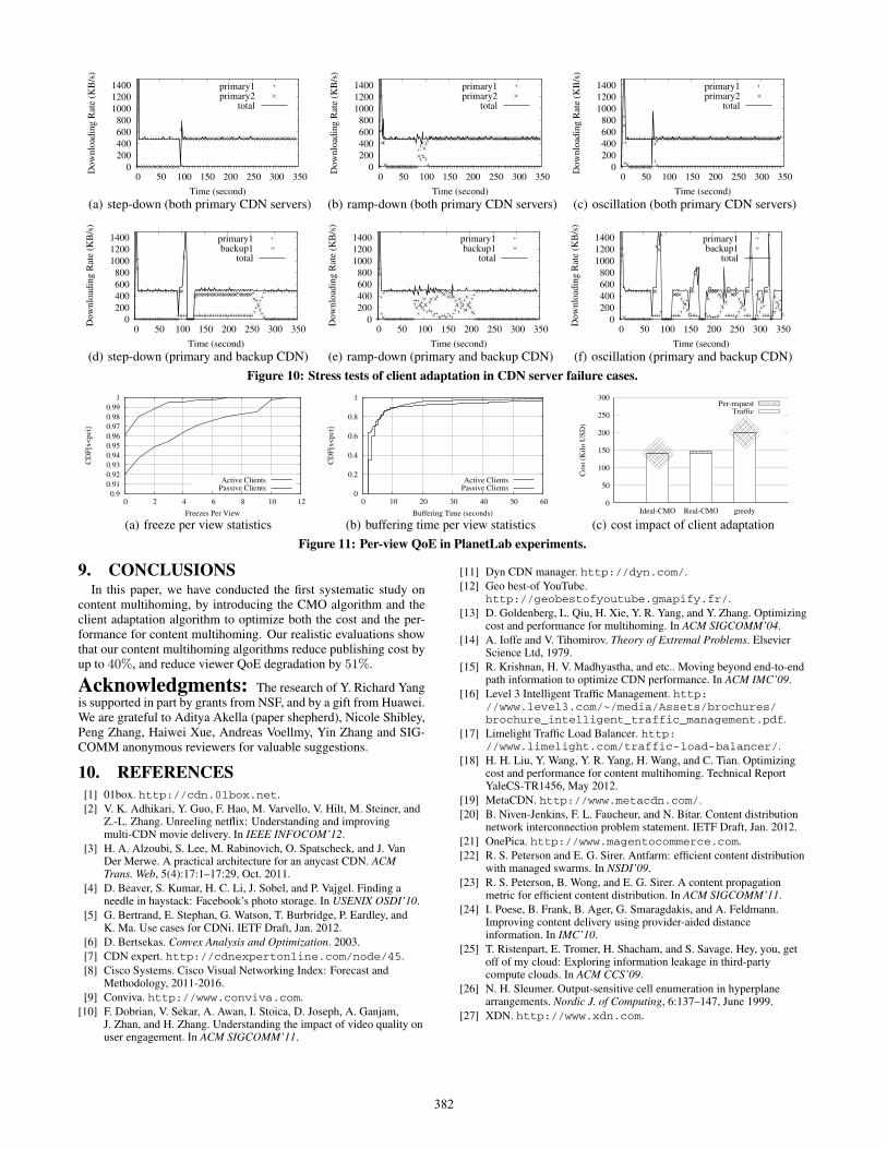
0 200 400 600 800

1000 1200 1400

0 50 100 150 200 250 300 350

Dow

nloa

ding

Rat

e (K

B/s

)

Time (second)

primary1primary2

total

(a) step-down (both primary CDN servers)

0 200 400 600 800

1000 1200 1400

0 50 100 150 200 250 300 350

Dow

nloa

ding

Rat

e (K

B/s

)

Time (second)

primary1primary2

total

(b) ramp-down (both primary CDN servers)

0 200 400 600 800

1000 1200 1400

0 50 100 150 200 250 300 350

Dow

nloa

ding

Rat

e (K

B/s

)

Time (second)

primary1primary2

total

(c) oscillation (both primary CDN servers)

0 200 400 600 800

1000 1200 1400

0 50 100 150 200 250 300 350

Dow

nloa

ding

Rat

e (K

B/s

)

Time (second)

primary1backup1

total

(d) step-down (primary and backup CDN)

0 200 400 600 800

1000 1200 1400

0 50 100 150 200 250 300 350D

ownl

oadi

ng R

ate

(KB

/s)

Time (second)

primary1backup1

total

(e) ramp-down (primary and backup CDN)

0 200 400 600 800

1000 1200 1400

0 50 100 150 200 250 300 350

Dow

nloa

ding

Rat

e (K

B/s

)

Time (second)

primary1backup1

total

(f) oscillation (primary and backup CDN)

Figure 10: Stress tests of client adaptation in CDN server failure cases.

0.9 0.91 0.92 0.93 0.94 0.95 0.96 0.97 0.98 0.99

1

0 2 4 6 8 10 12

CD

F[x<

pct]

Freezes Per View

Active ClientsPassive Clients

(a) freeze per view statistics

0

0.2

0.4

0.6

0.8

1

0 10 20 30 40 50 60

CD

F[x<

pct]

Buffering Time (seconds)

Active ClientsPassive Clients

(b) buffering time per view statistics

0

50

100

150

200

250

300

Ideal-CMO Real-CMO greedy

Cos

t (K

ilo U

SD)

Per-requestTraffic

(c) cost impact of client adaptation

Figure 11: Per-view QoE in PlanetLab experiments.

9. CONCLUSIONSIn this paper, we have conducted the first systematic study on

content multihoming, by introducing the CMO algorithm and theclient adaptation algorithm to optimize both the cost and the per-formance for content multihoming. Our realistic evaluations showthat our content multihoming algorithms reduce publishing cost byup to 40%, and reduce viewer QoE degradation by 51%.

Acknowledgments: The research of Y. Richard Yangis supported in part by grants from NSF, and by a gift from Huawei.We are grateful to Aditya Akella (paper shepherd), Nicole Shibley,Peng Zhang, Haiwei Xue, Andreas Voellmy, Yin Zhang and SIG-COMM anonymous reviewers for valuable suggestions.

10. REFERENCES[1] 01box. http://cdn.01box.net.[2] V. K. Adhikari, Y. Guo, F. Hao, M. Varvello, V. Hilt, M. Steiner, and

Z.-L. Zhang. Unreeling netflix: Understanding and improvingmulti-CDN movie delivery. In IEEE INFOCOM’12.

[3] H. A. Alzoubi, S. Lee, M. Rabinovich, O. Spatscheck, and J. VanDer Merwe. A practical architecture for an anycast CDN. ACMTrans. Web, 5(4):17:1–17:29, Oct. 2011.

[4] D. Beaver, S. Kumar, H. C. Li, J. Sobel, and P. Vajgel. Finding aneedle in haystack: Facebook’s photo storage. In USENIX OSDI’10.

[5] G. Bertrand, E. Stephan, G. Watson, T. Burbridge, P. Eardley, andK. Ma. Use cases for CDNi. IETF Draft, Jan. 2012.

[6] D. Bertsekas. Convex Analysis and Optimization. 2003.[7] CDN expert. http://cdnexpertonline.com/node/45.[8] Cisco Systems. Cisco Visual Networking Index: Forecast and

Methodology, 2011-2016.[9] Conviva. http://www.conviva.com.

[10] F. Dobrian, V. Sekar, A. Awan, I. Stoica, D. Joseph, A. Ganjam,J. Zhan, and H. Zhang. Understanding the impact of video quality onuser engagement. In ACM SIGCOMM’11.

[11] Dyn CDN manager. http://dyn.com/.[12] Geo best-of YouTube.

http://geobestofyoutube.gmapify.fr/.[13] D. Goldenberg, L. Qiu, H. Xie, Y. R. Yang, and Y. Zhang. Optimizing

cost and performance for multihoming. In ACM SIGCOMM’04.[14] A. Ioffe and V. Tihomirov. Theory of Extremal Problems. Elsevier

Science Ltd, 1979.[15] R. Krishnan, H. V. Madhyastha, and etc.. Moving beyond end-to-end

path information to optimize CDN performance. In ACM IMC’09.[16] Level 3 Intelligent Traffic Management. http:

//www.level3.com/~/media/Assets/brochures/brochure_intelligent_traffic_management.pdf.

[17] Limelight Traffic Load Balancer. http://www.limelight.com/traffic-load-balancer/.

[18] H. H. Liu, Y. Wang, Y. R. Yang, H. Wang, and C. Tian. Optimizingcost and performance for content multihoming. Technical ReportYaleCS-TR1456, May 2012.

[19] MetaCDN. http://www.metacdn.com/.[20] B. Niven-Jenkins, F. L. Faucheur, and N. Bitar. Content distribution

network interconnection problem statement. IETF Draft, Jan. 2012.[21] OnePica. http://www.magentocommerce.com.[22] R. S. Peterson and E. G. Sirer. Antfarm: efficient content distribution

with managed swarms. In NSDI’09.[23] R. S. Peterson, B. Wong, and E. G. Sirer. A content propagation

metric for efficient content distribution. In ACM SIGCOMM’11.[24] I. Poese, B. Frank, B. Ager, G. Smaragdakis, and A. Feldmann.

Improving content delivery using provider-aided distanceinformation. In IMC’10.

[25] T. Ristenpart, E. Tromer, H. Shacham, and S. Savage. Hey, you, getoff of my cloud: Exploring information leakage in third-partycompute clouds. In ACM CCS’09.

[26] N. H. Sleumer. Output-sensitive cell enumeration in hyperplanearrangements. Nordic J. of Computing, 6:137–147, June 1999.

[27] XDN. http://www.xdn.com.

382