Optimizing Bank Overdraft Fees with Big Data

Xiao Liu, Alan L. Montgomery, Kannan Srinivasan

Working Paper

June 2016

Xiao Liu (xliu@stern.nyu.edu) is an Assistant Professor of Marketing at the Stern School of Business at New York University, Alan L. Montgomery (alanmontgomery@cmu.edu) is an Associate Professor of Marketing at the Tepper School of Business at Carnegie Mellon University, and Kannan Srinivasan (kannans@cmu.edu) is the H.J. Heinz II Professor of Management, Marketing and Information Systems at the Tepper School of Business at Carnegie Mellon University. Xiao Liu acknowledges support from the Dipankar and Sharmila Chakravarti Fellowship. We thank the financial services firm that provided the data. Any opinions, findings, conclusions and recommendations expressed in this paper are those of the author(s) and not of our sponsors.

Copyright © 2016 by Xiao Liu, Alan L. Montgomery and Kannan Srinivasan. All rights reserved

Optimizing Bank Overdraft Fees with Big Data

Abstract

In 2012, consumers paid $32 billion in overdraft fees, representing the single largest source of revenue for

banks from demand deposit accounts during this period. Owing to consumer attrition caused by overdraft

fees and potential government regulations to reform these fees, financial institutions have become motivated

to investigate their overdraft fee structures. Banks need to balance the revenue generated from overdraft fees

with consumer dissatisfaction and potential churn caused by these fees. However, no empirical research has

been conducted to explain consumer responses to overdraft fees or to evaluate alternative pricing and

product strategies associated with these fees. In this research, we propose a dynamic structural model with

consumer monitoring costs and dissatisfaction associated with overdraft fees. We find that consumers heavily

discount the future and potentially overdraw because of impulsive spending. However, we also find that high

monitoring costs hinder consumers’ effort to track their balance accurately; consequently, consumers may

overdraw because of rational inattention. We apply the model to an enterprise-level dataset of more than

500,000 accounts with a history of 450 days, providing a total of 200 million transactions. This large dataset is

necessary because of the infrequent nature of overdrafts; however, it also engenders computational challenges,

which we address by using parallel computing techniques. Our policy simulations show that alternative

pricing strategies may increase bank revenue and improve consumer welfare.

Keywords: Banking, Overdraft Fees, Dynamic Programming, Big Data.

- 1 -

1 Introduction

An overdraft occurs when a consumer spends or withdraws an amount of funds from his or her

checking account that exceeds the account’s available funds. US banks allow consumers to overdraw their

account (subject to some restrictions at the bank’s discretion) but charge an overdraft fee. Overdraft fees

have been a major source of bank revenue since the early 1980s1, when banks started to offer free checking

accounts to attract consumers. According to Moebs Services, the total amount of overdraft fees in the US

reached $32 billion in 2012. This is equivalent to an average of $178 for each checking account annually2.

According to the Center for Responsible Lending, US households spent more on overdraft fees than on fresh

vegetables, postage or books in 20103.

Overdraft fees have provoked a storm of consumer outrage and can induce many consumers who

experience these fees to close their account4. The US government has taken actions to regulate overdraft fees

through the Consumer Financial Protection Agency5, and it may take more drastic steps in the future6. From

the banks’ perspective, consumer defaults on overdrafted accounts can result in billions in charge offs.

Therefore, there are pressures throughout the industry for banks to reexamine their overdraft fee practices.

From a strategic perspective, banks need to be able to find alternative sources of revenue to be able to

profitably provide basic financial services such as checking accounts instead of being highly reliant on

unpopular overdraft fees.

A potential solution for both consumers and banks is to leverage financial transaction data to manage

overdrafting and offer new services using these financial transaction data. Financial institutions store massive

1 Topper, S. The History and Evolution of the Free Checking Account. [Web log comment]. Retrieved from http://freecheckinginformation.com/financial-writers/the-history-and-evolution-of-the-free-checking-account/ 2 According to Evans, Litan, and Schmalensee (2011), there are 180 million checking accounts in the US. 3 Burns, R. (2010). Managing Credit: 3 Ways Overdraft Fees Will Still Haunt You. Retrieved from http://www.blackenterprise.com/money/managing-credit-3-ways-overdraft-fees-will-still-haunt-you/ 4 Examples can be found at http://consumersunion.org/2013/06/rep-carolyn-maloney-pursues-consumer-protections-on-overdraft-fees/ and http://america.aljazeera.com/watch/shows/real-money-with-alivelshi/Real-Money-Blog/2014/1/21/overdraft-fee-abuse.html. 5 Consumers and Congress Tackle Big Bank Fees. Retrieved from http://banking-law.lawyers.com/consumer-banking/consumers-and-congress-tackle-big-bank-fees.html 6 Consumer Financial Protection Bureau. (2013). CFPB Study of Overdraft Programs. Retrieved from http://files.consumerfinance.gov/f/201306_cfpb_whitepaper_overdraft-practices.pdf

- 2 -

amounts of information about consumers, commonly referred to as Big Data, as a byproduct of their

transactions. In this research, we show how this information can be harnessed with structural economic

theories to predict consumers’ overdrafting behavior. The large-scale of our financial transaction panel data

allows us to detect rare events of overdrafts, identify rich consumer heterogeneity and minimize sampling bias

to avoid potential financial losses. Consequently, we propose personalized strategies that can increase both

consumer welfare and bank revenue. Our goal is to show that the knowledge about consumers contained

within their financial transaction data can form the basis for improving customer welfare and increasing

profitability for the bank by tapping into this underutilized resource for marketing purposes.

In this paper, we have two substantive goals. First, we wish to show how financial institutions can

leverage the rich data on consumer spending and balance checking to understand the decision process

underlying consumers’ overdrafting behavior. We address the following research questions: Why do

consumers overdraw? How do consumers react to overdraft fees? Second, we investigate alternative pricing

strategies that optimize overdraft fees. Specifically, we tackle the following questions: Is the current overdraft

fee structure optimal? How will bank revenue and consumer welfare change under alternative pricing

strategies?

In answering these questions, we make two key methodological contributions. First, we construct a

dynamic structural model that incorporates inattention and dissatisfaction into the life-time consumption

model. Structural models have the merit of producing policy-invariant parameters that allow us to conduct

counterfactual analyses. However, the inherent computational burden prevents them from being widely

adopted by the industry. This leads to our second key contribution, whereby we show how to estimate a

structural model applied to Big Data with the help of parallel computing techniques. Our proposed algorithm

takes advantage of state-of-the-art parallel computing techniques and estimation methods to lessen the

computational burden and reduce the curse of dimensionality to the point where near-real-time results are

possible. We estimate our dynamic structural model using anonymized data from a large US bank. The data

include over 500,000 accounts with a history of up to 450 days, amounting to 200 million relevant

observations. This enterprise-level dataset is much larger than those reported in other research studies.

- 3 -

Substantively, we find that some consumers are inattentive in monitoring their balance because of the

associated high monitoring costs. In contrast, attentive consumers primarily overdraw because they heavily

discount future utilities and are subject to impulsive spending. Consumers who are dissatisfied may then leave

their bank after being charged high overdraft fees. In our counterfactual analysis, we show that a percentage

fee or a quantity premium fee strategy can achieve higher bank revenue than the current flat per-transaction

fee strategy. Consumers also benefit from the lowered overdraft fees by improving their capabilities to

smooth out consumption over time and save monitoring costs.

The rest of the paper is organized as follows. In §2, we review related research. We report an

exploratory data analysis in §3 to motivate our model setup. §4 describes our structural model. Details about

the identification and estimation procedures are given in §5. §6 and §7 discuss our estimation results and

counterfactual analysis. §8 concludes with a discussion of our findings and the limitations of our research.

2 Literature Review

An economic approach to explaining overdrafting would assume that consumers are rational and

forward-looking with an objective to maximize their total discounted utility by making optimal choices

(Modigliani and Brumberg 1954, Hall 1978). Consistent with the rational argument for overdrafting is that

consumers heavily discount the future and are willing to pay future overdraft fees in to allow consumption

today. While we are sympathetic to full-information rational models of consumer behavior, we do not want

to overlook potential behavioral explanations of overdrafting behavior. Specifically, we consider two novel

arguments that offer behavioral explanations concerning overdrafting: inattention and dissatisfaction.

The inattention argument is present in a large body of literature in psychology and economics, which

has found that consumers pay limited attention to relevant information. In their review paper, DellaVigna

(2009) summarize findings indicating that consumers pay limited attention to 1) shipping costs, 2) tax (Chetty

et. al. 2009) and 3) rankings (Pope 2009). Gabaix and Laibson (2006) find that consumers do not pay enough

attention to add-on pricing, and Grubb (2014) shows that consumers are inattentive to their cell-phone

minute balances. Many papers in finance and accounting have documented that investors and financial

- 4 -

analysts are inattentive to various types of financial information (e.g., Hirshleifer and Teoh 2003, Peng and

Xiong 2006).

Stango and Zinman (2014) consider limited attention as an explanation of overdrafting. They define

inattention as incomplete consideration of account balances (realized balance and available balance net of

upcoming bills) that would inform choices. Although Stango and Zinman (2014) use a dataset similar to ours,

their aim is to show that reminding participants about overdraft fees can reduce the likelihood of overdrafts.

We adopt this definition of inattention, but we introduce inattention through a structural parameter, the

monitoring cost (Reis 2006), which represents the time and effort required for a consumer to know the exact

amount of money in his or her checking account.

A second behavioral argument related to overdrafting is that it may cause consumer dissatisfaction.

The implied interest rate for an overdraft originated by a small transaction amount implies usurious rates that

are much higher than the socially accepted interest rate (Matzler, Wurtele and Renzl 2006), leading to price

dissatisfaction. This is because under current banking practices, consumers pay flat per-transaction fees

regardless of the transaction amount. Overdrafting fees may cause consumer dissatisfaction, which is one of

the main causes of customer switching behavior (Keaveney 1995, Bolton 1998). We conjecture that

consumers are likely to close their account after they pay an overdraft fee and/or if the ratio of the overdraft

fee to the overdraft transaction amount is high. Before posing a formal economic model, we begin with the

data and an exploratory data analysis to validate whether there is evidence for high discounting, inattention

and dissatisfaction.

3 Data

We obtain anonymized data from a large US bank. Our data comprise bank transaction data for a

sample of more than 500,000 accounts7 with more than 200 million transactions over a fifteen-month period

(June 2012 to Aug 2013). These data are a by-product of consumers’ financial transactions. For each

7 For the sake of confidentiality, we cannot disclose the exact number, but it is a representative sample from the banks’ customers and is within the range of 500,000 to 1,000,000 accounts.

- 5 -

transaction, we know the account number, associated customer information, date, channel, amount, and type.

Table 1 provides a simulated example of the raw information for a consumer. In this example, the consumer

makes an ATM withdrawal and starts with a positive balance. On the next day, a check is paid by the bank

even though the consumer has insufficient funds, which triggers an overdraft and the corresponding fee. A

direct deposit from salary income is received, which brings the consumer’s balance to a positive amount.

Subsequently, the consumer does a balance check and makes a purchase at the supermarket on the next day.

The description in this example is given for illustrative purposes and is not provided in our dataset. Each

transaction is classified into one of five categories: bills, fees assessed by the bank, income (from deposits and

transfers), spending, and balance inquiries.

Date Description Channel Type +/- Amount Balance

11/14/12 ATM withdrawal ATM Spending - $80.00 $63.15

11/15/12 Check cashed for electric payment ACH Bill - $130.41 -$67.26

11/15/12 Overdraft item fee Fee - $31.00 -$98.26

11/16/12 Salary from direct deposit ACH Income + $287.42 $189.16

11/17/12 Check balance ATM Balance Inquiry o $189.16

11/17/12 Debit card purchase at supermarket Debit Spending - $97.84 $91.32

Table 1. Example of Simulated Transaction Data for an Individual.

The bank in the dataset provides a comprehensive set of services for consumers to avoid overdrafts,

such as automatic transfers, but despite these offerings, a significant number of consumers still overdraw.

(For a good review of general overdraft practices in the US, refer to Stango and Zinman (2014). Appendix

A1 tabulates the current fee settings of the top US banks.) If a consumer overdraws his or her account with

the standard overdraft service, then the bank might cover the transaction and charge a $318 Overdraft Fee

(OD) or decline the transaction and charge a $31 Non-Sufficient-Fund Fee (NSF). The bank can accept or

decline the transaction at its discretion. The OD/NSF is applied at a per-item level: if a consumer performs

several transactions when his or her account is already overdrawn, each transaction item will incur a fee of

$31. However, within a day, a maximum of four per-item fees can be charged. If the account remains

8 All dollar values in the paper have been rescaled by a number between .85 and 1.15 to help obfuscate the exact amounts and preserve the anonymity of the customers, but this factor does not change the substantive implications. Using our rescaled values the bank sets the first-time overdraft fee for each consumer at $22, and all subsequent overdraft fees are set at $31.

- 6 -

overdrawn for five or more consecutive calendar days, a Continuous Overdraft Fee of $6 is assessed up to a

maximum of $84. The bank also provides an Overdraft Protection Service where a checking account can be

linked to another checking account, a credit card or a line of credit. In this case, when the focal account is

overdrawn, funds can be transferred to cover the negative balance. The Overdraft Transfer Balance Fee is $9

for each transfer. In summary, the overdraft fee structure for the bank, as for most others, is quite

complicated. In our empirical analysis, we do not distinguish among different types of overdraft fees, and we

assume that consumers care only about the total amount of overdraft fees rather than the underlying pricing

structure.

The bank also provides balance checking services through its branches, automated teller machines

(ATMs), call centers and online/mobile banking service. Consumers can inquire about their available balances

and recent activities. There is also a notification service, so-called “alerts”, that notifies consumers via emails

or text messages when certain events take place, such as overdrafts, incidents of insufficient funds, transfers,

and deposits. Unfortunately, our dataset includes only balance checking data, not alert data. We discuss this

limitation in §8.

In 2009, the Federal Reserve Board made an amendment to Regulation E (subsequently recodified by

the Consumer Financial Protection Bureau (CFPB)), which requires account holders to provide affirmative

consent (opt-in) for overdraft coverage of ATM and nonrecurring point-of-sale (POS) debit card transactions

before banks can charge consumers for paying such transactions9. Regulation E was intended to protect

consumers from heavy overdraft fees. The change became effective for new accounts on July 1, 2010, and for

existing accounts on August 15, 2010. Our data contain both opt-in and opt-out accounts. However, we do

not know which accounts have opted-in unless we observe an ATM/POS-initiated overdraft incident. We

discuss this data limitation in §8.

9 Electronic Fund Transfer Act. Retrieved from http://www.federalreserve.gov/bankinforeg/caletters/Attachment_CA_13-17_Reg_E_Examination_Procedures.pdf

- 7 -

3.1 Descriptive Statistics

In our dataset, overdraft fees accounted for 47% of the revenue from deposit account service

charges and 9.8% of the operating revenue. In all, 15.8% of accounts had at least one overdraft incident. The

proportion of accounts with overdrafts is lower than the 27% (across all banks and credit unions) reported by

the CFPB in 201210. Table 2 shows that consumers who paid overdraft fees overdrew nearly 10 times and

paid $245 on average during the 15-month sample period. This is consistent with the finding from the CFPB

that the average overdraft- and NSF-related fees paid by all accounts with one or more overdraft transactions

in 2011 totaled $225 11 . There is significant heterogeneity in consumers’ overdraft frequency, and the

distribution of overdraft frequency is quite skewed. The median overdraft frequency is three, and more than

25% of consumers overdrew only once. In contrast, the top 0.15% of the heaviest overdrafters overdrew

more than 100 times. A similar skewed pattern is observed for the distribution of overdraft fees. While the

median overdraft fee is $77, the top 0.15% of heaviest overdrafters paid more than $2,730 in fees.

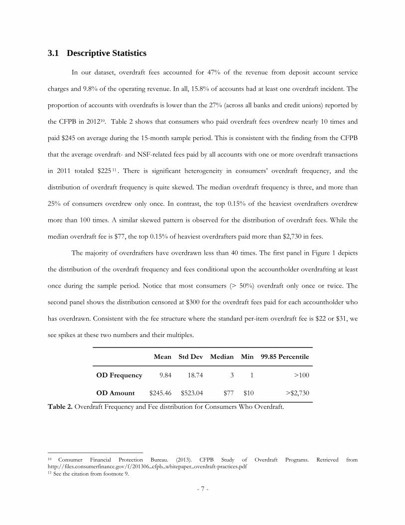
The majority of overdrafters have overdrawn less than 40 times. The first panel in Figure 1 depicts

the distribution of the overdraft frequency and fees conditional upon the accountholder overdrafting at least

once during the sample period. Notice that most consumers (> 50%) overdraft only once or twice. The

second panel shows the distribution censored at $300 for the overdraft fees paid for each accountholder who

has overdrawn. Consistent with the fee structure where the standard per-item overdraft fee is $22 or $31, we

see spikes at these two numbers and their multiples.

Mean Std Dev Median Min 99.85 Percentile

OD Frequency 9.84 18.74 3 1 >100

OD Amount $245.46 $523.04 $77 $10 >$2,730

Table 2. Overdraft Frequency and Fee distribution for Consumers Who Overdraft.

10 Consumer Financial Protection Bureau. (2013). CFPB Study of Overdraft Programs. Retrieved from http://files.consumerfinance.gov/f/201306_cfpb_whitepaper_overdraft-practices.pdf 11 See the citation from footnote 9.

- 8 -

Figure 1. Overdraft Frequency and Fee Distribution.

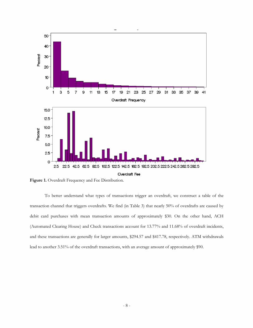
To better understand what types of transactions trigger an overdraft, we construct a table of the

transaction channel that triggers overdrafts. We find (in Table 3) that nearly 50% of overdrafts are caused by

debit card purchases with mean transaction amounts of approximately $30. On the other hand, ACH

(Automated Clearing House) and Check transactions account for 13.77% and 11.68% of overdraft incidents,

and these transactions are generally for larger amounts, $294.57 and $417.78, respectively. ATM withdrawals

lead to another 3.51% of the overdraft transactions, with an average amount of approximately $90.

- 9 -

Type Frequency Percentage Amount

Debit Card Purchase 946,049 48.65% $29.50

ACH Transaction 267,854 13.77% $294.57

Check 227,128 11.68% $417.78

ATM Withdrawal 68,328 3.51% $89.77

Table 3. Types of Transactions That Cause Overdraft

3.2 Exploratory Data Analysis

This section presents some patterns in the data that suggest the causes and effects of overdrafts. We

show that heavy discounting and inattention may drive consumers’ overdrafting behavior and that consumers

are dissatisfied because of overdraft fees. The model-free evidence also highlights the variation in the data

that will allow for the identification of the discount factor, monitoring cost and dissatisfaction sensitivity.

3.2.1 Heavy Discounting

First, we conjecture that a consumer may overdraw because of a much greater preference for current

consumption than future consumption, i.e., the consumer heavily discounts future consumption utility. At the

point of sale, such a consumer sharply discounts the future cost of the overdraft fee to satisfy his or her

immediate gratification 12 . In such a case, we should observe a steep downward sloping trend in the

consumer’s spending pattern within a pay period. That is, the consumer will increase spending right after he

or she receives a pay check and will then reduce spending over the course of the month. However, because of

his or her overspending at the beginning of the month, the consumer will run out of funds at the end of the

pay period and have to overdraw.

We test this hypothesis with the following model of spending for consumer at time :

∗

12 We also considered hyperbolic discounting with two discount factors, a short-term present bias parameter and a long-term discount factor. With more than three periods of data within a pay period, hyperbolic discount factors can be identified (Fang and Silverman 2009). However, our estimation results show that the present bias parameter is not significantly different from 1. Therefore, we keep only one discount factor in the current model. Estimation results with hyperbolic discount factors are available upon request.

- 10 -

where is the number of days after the consumer received income (salary), is

the individual fixed effect and is the time (day) fixed effect. To control for the effect that consumers

usually pay for their bills (utilities, phone bills, credit card bills, etc.) after receiving their paycheck, we exclude

checks and ACH transactions, which are the common choices for bill payments from daily spending and keep

only debit card purchases, ATM withdrawals and person-to-person transfers.

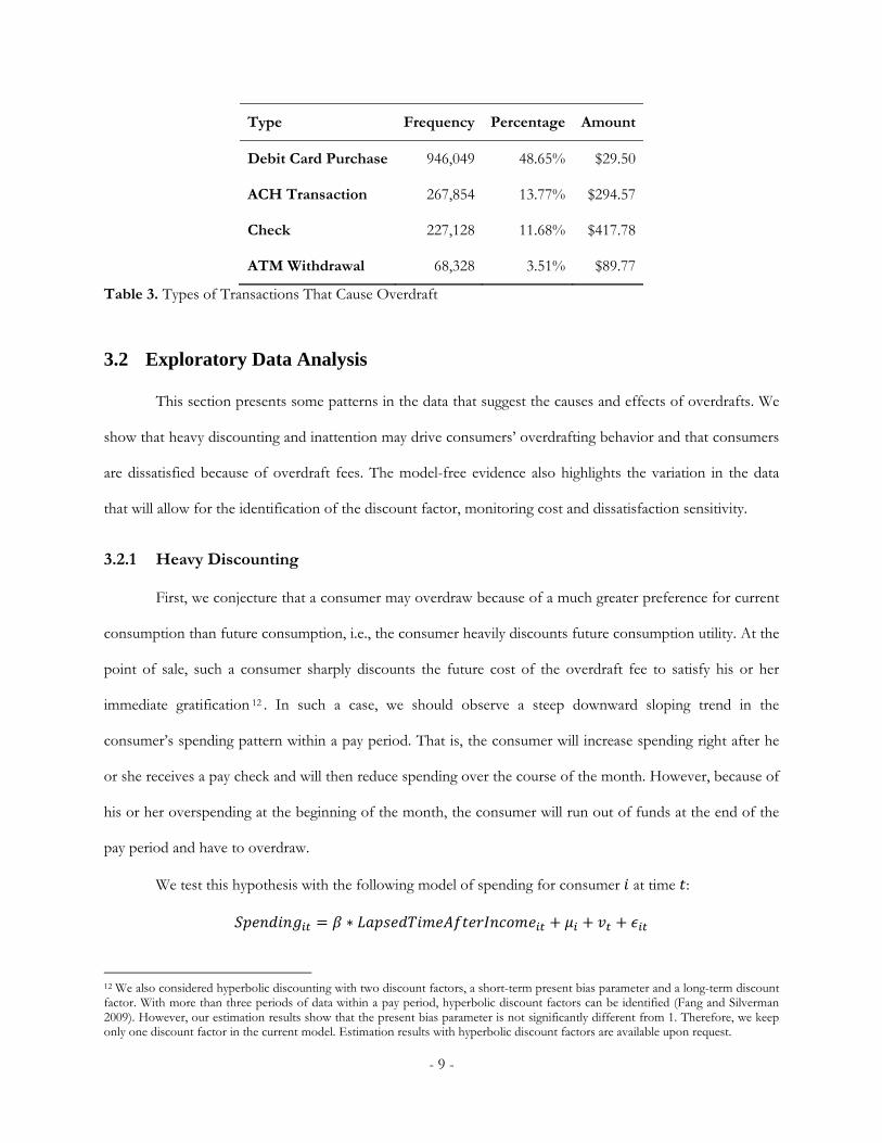
We run this OLS regression separately for heavy overdrafters (whose overdraft frequencies are in the

top 20 percentile of all overdrafters), light overdrafters (whose overdraft frequencies are not in the top 20

percentile) and non-overdrafters (who do not overdraw during the 15-month sample period)13. The results are

reported in columns (1), (2) and (3) of Table 4.

(1) (2) (3)

Heavy

OverdraftersLight

OverdraftersNon-

OverdraftersLapsed Time after Income ( ) -6.8374*** -0.07815 -0.02195 (0.06923) (0.06540) (0.02328)Fixed Effect Yes Yes YesNumber of Observations 17,810,276 53,845,039 242,598,851R2 0.207 0.275 0.280Note: *p<0.01;**p<0.001;***p<0.0001

Table 4. Spending Decreases with Time in a Pay Cycle

We find that the coefficient of is negative and significant for heavy

overdrafters but not light overdrafters or non-overdrafters. This suggests that heavy overdrafters have a steep

downward sloping spending pattern during a pay period, while light overdrafters or non-overdrafters have a

relatively stable spending stream. The heavy overdrafters are likely to overdraw because of their heavy

discounting of future consumption.

3.2.2 Inattention

Next, we consider why light overdrafters may overdraft due to inattention. The idea is that

consumers might not always monitor their account balance and may be uncertain about the exact balance

13 We separate the analyses for heavy/light/non-overdrafters because each segment shows distinct behavioral patterns. The segment is defined by the number of overdraft occurrences in the sample period. It is also interesting to investigate the demographic variables that characterize these three segments of consumers. The results are presented in Appendix A5.

- 11 -

amount. Sometimes, the perceived balance can be higher than the true balance, and this might cause an

overdraft. We first present a representative example of consumer inattention. The example is based on our

data, but to protect the privacy of the consumer and the merchants, the amounts have been changed.

However, the example remains representative of the underlying data.

Figure 2. Overdraft due to a Balance Perception Error

As shown in Figure 2, the consumer first received his or her bi-weekly salary on August 17th. After a

series of expenses, the consumer is left with $21.16 on August 20th. The consumer did not check his or her

balance but continued spending and overdrew the account for several small purchases, including a $25

restaurant bill, a $17.12 beauty purchase, a $6.31 game and a $4.95 coffee purchase. These four transactions

totaled only $53.38 but caused the consumer to pay four overdraft item fees for total fees of $124. We

speculate that this consumer was careless in monitoring his or her account and overestimated his or her

balance.

- 12 -

Beyond this example, we find more evidence of inattention in the data. To start off, Table 3 suggests

that debit card purchases cause the most overdraft incidences, perhaps because it is more difficult to check

balances when using a debit card than using an ATM or ACH.

Moreover, intuitively, as direct support of our hypothesis regarding inattention, the less frequently a

consumer checks his or her balance, the more overdraft fees the consumer will likely incur. To test this

hypothesis, we estimate the following specification:

where is the total overdraft payment and is the balance checking frequency for

consumer at time (month).

We estimate this model on light overdrafters (whose overdraft frequency is not in the top 20

percentile) and heavy overdrafters (whose overdraft frequency is in the top 20 percentile) separately and

report the result in columns (1) and (2) in Table 5.

(1) (2) (3)

Light

OverdraftersHeavy

Overdrafters All

OverdraftersBalance Checking Frequency ( , ) -0.5001*** -0.1389 -0.6823*** 0.0391 0.0894 0.0882 Overdraft Frequency ( , ) 16.0294*** 0.2819

∗ ( ) 0.278136*** 0.0607Number of Observations 1,794,835 593,676 2,388,511

0.1417 0.1563 0.6742 Note: Fixed effects at the individual and day level; robust standard errors clustered at the individual level. *p<0.01;**p<0.001;***p<0.0001

Table 5. Frequent Balance Checking Reduces Overdrafts for Light Overdrafters

The result suggests that a higher frequency of balance checking decreases the overdraft payment for

light overdrafters but not for heavy overdrafters. We further test this effect by including the overdraft

frequency ( ) and an interaction term for balance checking frequency and overdraft frequency

∗ in the equation below. The idea is that if the coefficient for this interaction term is

positive while the coefficient for balance checking frequency ( ) is negative, then it implies that a

- 13 -

high frequency of balance checking decreases overdraft fees only for consumers who overdraw infrequently,

not for those who overdraw frequently.

∗

The results in column (3) of Table 5 confirm our hypothesis14.

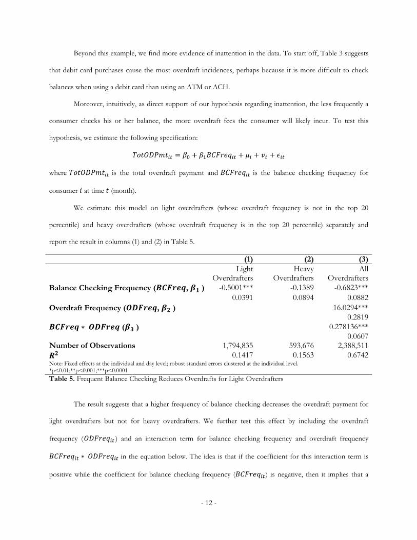
Interestingly, we find that consumers’ balance perception error accumulates over time in the sense

that the greater the time elapsed without checking their balance, the more likely they are to overdraw and

consequently pay higher amounts in overdraft fees. Figure 3 below exhibits the overdraft probability across

the number of days elapsed since the last time a consumer checked his or her balance for light overdrafters

(whose overdraft frequency is not in the top 20 percentile). As the figure shows, the overdraft probability

increases moderately with the number of days elapsed since the last balance check.

Figure 3. Overdraft Likelihood Increases with Time Elapsed Since the Last Balance Check

We confirm this relationship with the following two specifications. We assume that the overdraft

incidence (where 1 denotes overdraft and 0 denotes no overdraft) and

overdraft fee payment amount for consumer at time can be modeled as:

Φ

14 We also find that light overdrafters are more likely to check balances after overdraft fees are charged than heavy overdrafters. This also provides evidence for inattention. Furthermore, we find that light overdrafters fail to learn from past experiences. Specifically, we find a positive correlation between the time elapsed since overdraft and the time gap between two balance checking times. This suggests that immediately after overdrafting, consumers might start monitoring their checking accounts. As time goes by, however, they become inattentive again.

- 14 -

where Φ is the cumulative distribution function for a standard normal distribution. The term

denotes the number of days that consumer has not checked his or her

balance until time and is the beginning balance at time . We control for the beginning balance

because it may be negatively correlated with the days elapsed since last balance check because consumers tend

to check their balance when it is low, and a lower balance often leads to an overdraft. Table 6 reports the

estimation results, which support our hypothesis that the greater the time elapsed after a balance check, the

more likely the consumer is to overdraw and incur higher overdraft fees.

I (OD) ODFeeDays Since Last Balance Check ( ) 0.0415*** 0.0003*** (0.0027) (0.0001)Beginning Balance ( ) -0.7265*** -0.0439*** (0.0066) (0.0038)Individual Fixed Effect Yes YesTime Fixed Effect Yes YesNumber of Observations 53,845,039 53,845,039R2 0.5971 0.6448Note: The estimation sample includes only overdrafters. Marginal effects for the Probit model; Fixed effects at the individual and day level; robust standard errors clustered at the individual level.*p<0.01;**p<0.001;***p<0.0001.

Table 6. Reduced-Form Evidence of the Existence of Monitoring Costs

If balance checking can help prevent overdrafts, why do consumers not check their balance more

frequently and avoid overdraft fees? We argue that monitoring their account balance is costly in terms of time,

effort and mental resources, which reduces the number of balance checks. We expect that if there were a way

for consumers to save their time, effort or mental resources, then they would check their balance more

frequently. We find support for this expectation with consumers who use online banking. Specifically, for

consumer , we estimate the following specification:

where is the balance checking frequency, is online banking ownership (1

denotes that the consumer has online banking, while 0 denotes otherwise), is whether the

consumer belongs to the low-income group (1 denotes yes and 0 denotes no), and is age (in years).

Table 7 shows that after controlling for income and age, consumers with online banking accounts check their

- 15 -

balance more frequently than those without online banking accounts, which suggests that monitoring costs

exist and that consumers monitor their account more frequently when these costs are reduced.

Dependent variable Check Balance FrequencyOnline Banking ( ) 58.4245*** 0.5709Low Income ( ) 3.3812*** 0.4178Age ( ) 0.6474*** 0.0899Number of Observations 602,481R2 0.6448*p<0.01;**p<0.001;***p<0.0001.

Table 7. Reduced-Form Evidence of Existence of Monitoring Cost

3.2.3 Dissatisfaction

We find that overdrafts might cause consumers to close their account (Table 8). Among non-

overdrafters, 7.87% closed their account during the sample period. This ratio is much higher for overdrafters.

Specifically, 23.36% of heavy overdrafters (whose overdraft frequency is in the top 20 percentile) closed their

account, while 10.56% of light overdrafters (whose overdraft frequency is not in the top 20 percentile) closed

their account.

Total % ClosedHeavy Overdrafters 23.36%Light Overdrafters 10.56%Non-Overdrafters 7.87%

Table 8. Account Closure Frequency for Overdrafters vs Non-Overdrafters

From the description field associated with each account, we can distinguish the cause of account

closure: forced closure by the bank because the consumer is unable or unwilling to pay back the overdrawn

balance and fees (in which case the bank executes a charge-off) versus voluntary closure. Among heavy

overdrafters, 13.66% closed their account voluntarily, and the remaining 86.34% were forced by the bank to

close their account (Table 9). In contrast, 47.42% of the light overdrafters closed their account voluntarily.

We conjecture that the higher voluntary closures among light overdrafters may be due to customer

dissatisfaction with the bank, as the evidence below shows.

- 16 -

Overdraft Forced

ClosureOverdraft Voluntary

ClosureNo Overdraft

Voluntary ClosureHeavy Overdrafters 86.34% 13.66% -Light Overdrafters 52.58% 47.42% -Non-Overdrafters - - 100.00%

Table 9. Closure Reasons15

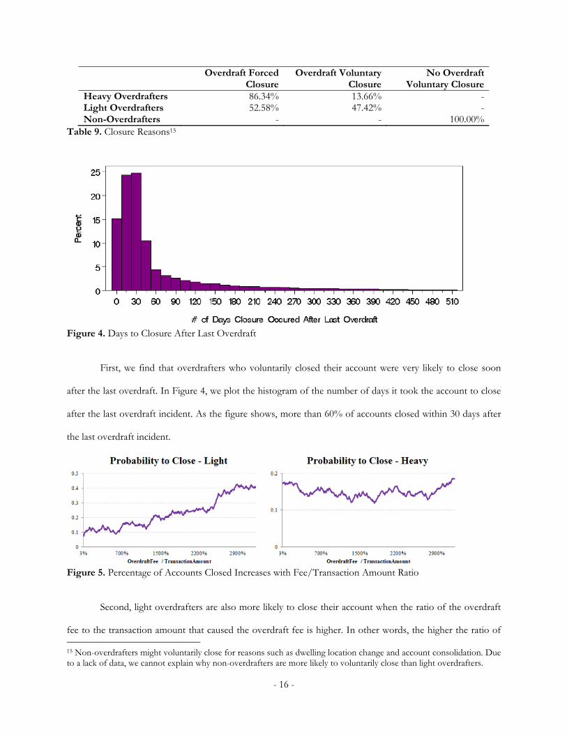
Figure 4. Days to Closure After Last Overdraft

First, we find that overdrafters who voluntarily closed their account were very likely to close soon

after the last overdraft. In Figure 4, we plot the histogram of the number of days it took the account to close

after the last overdraft incident. As the figure shows, more than 60% of accounts closed within 30 days after

the last overdraft incident.

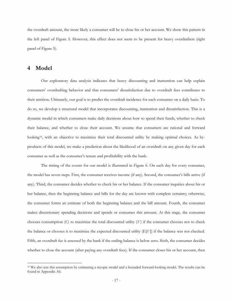
Figure 5. Percentage of Accounts Closed Increases with Fee/Transaction Amount Ratio

Second, light overdrafters are also more likely to close their account when the ratio of the overdraft

fee to the transaction amount that caused the overdraft fee is higher. In other words, the higher the ratio of 15 Non-overdrafters might voluntarily close for reasons such as dwelling location change and account consolidation. Due to a lack of data, we cannot explain why non-overdrafters are more likely to voluntarily close than light overdrafters.

- 17 -

the overdraft amount, the more likely a consumer will be to close his or her account. We show this pattern in

the left panel of Figure 5. However, this effect does not seem to be present for heavy overdrafters (right

panel of Figure 5).

4 Model

Our exploratory data analysis indicates that heavy discounting and inattention can help explain

consumers’ overdrafting behavior and that consumers’ dissatisfaction due to overdraft fees contributes to

their attrition. Ultimately, our goal is to predict the overdraft incidence for each consumer on a daily basis. To

do so, we develop a structural model that incorporates discounting, inattention and dissatisfaction. This is a

dynamic model in which consumers make daily decisions about how to spend their funds, whether to check

their balance, and whether to close their account. We assume that consumers are rational and forward

looking16, with an objective to maximize their total discounted utility by making optimal choices. As by-

products of this model, we make a prediction about the likelihood of an overdraft on any given day for each

consumer as well as the consumer’s tenure and profitability with the bank.

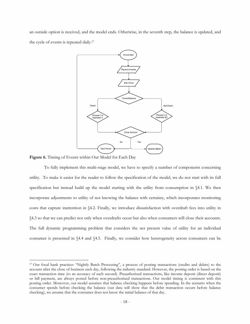
The timing of the events for our model is illustrated in Figure 6. On each day for every consumer,

the model has seven steps. First, the consumer receives income (if any). Second, the consumer’s bills arrive (if

any). Third, the consumer decides whether to check his or her balance. If the consumer inquiries about his or

her balance, then the beginning balance and bills for the day are known with complete certainty; otherwise,

the consumer forms an estimate of both the beginning balance and the bill amount. Fourth, the consumer

makes discretionary spending decisions and spends or consumes this amount. At this stage, the consumer

chooses consumption (C) to maximize the total discounted utility (V) if the consumer chooses not to check

the balance or chooses it to maximize the expected discounted utility (E[V]) if the balance was not checked.

Fifth, an overdraft fee is assessed by the bank if the ending balance is below zero. Sixth, the consumer decides

whether to close the account (after paying any overdraft fees). If the consumer closes his or her account, then

16 We also test this assumption by estimating a myopic model and a bounded forward-looking model. The results can be found in Appendix A6.

- 18 -

an outside option is received, and the model ends. Otherwise, in the seventh step, the balance is updated, and

the cycle of events is repeated daily.17

Figure 6. Timing of Events within Our Model for Each Day To fully implement this multi-stage model, we have to specify a number of components concerning

utility. To make it easier for the reader to follow the specification of the model, we do not start with its full

specification but instead build up the model starting with the utility from consumption in §4.1. We then

incorporate adjustments to utility of not knowing the balance with certainty, which incorporates monitoring

costs that capture inattention in §4.2. Finally, we introduce dissatisfaction with overdraft fees into utility in

§4.3 so that we can predict not only when overdrafts occur but also when consumers will close their accounts.

The full dynamic programming problem that considers the net present value of utility for an individual

consumer is presented in §4.4 and §4.5. Finally, we consider how heterogeneity across consumers can be

17 Our focal bank practices “Nightly Batch Processing”, a process of posting transactions (credits and debits) to the account after the close of business each day, following the industry standard. However, the posting order is based on the exact transaction time (to an accuracy of each second). Preauthorized transactions, like income deposit (direct deposit) or bill payment, are always posted before non-preauthorized transactions. Our model timing is consistent with this posting order. Moreover, our model assumes that balance checking happens before spending. In the scenario when the consumer spends before checking the balance (our data will show that the debit transaction occurs before balance checking), we assume that the consumer does not know the initial balance of that day.

- 19 -

specified in §4.6 to complete the full specification of the model. The estimation of the model is discussed in

the following section §5.

4.1 Consumption Model

At the core of our model is the need to predict consumers’ daily decisions about how much to

consume today versus in the future. Following the lifetime consumption literature (Modigliani and Brumberg

1954, Hall 1978), we assume that consumer ’s per-period consumption utility at time t is determined by a

constant relative risk averse (CRRA) utility function (Arrow 1963):

1(1)

where 18 is consumer ’s consumption at period and is the coefficient of relative risk aversion. We

choose the CRRA utility function because it has the merits of empirical support (Friend and Blume 1975),

analytical convenience (Merton 1992), and is commonly used in the economics literature. The coefficient of

relative risk aversion is always positive, and its inverse is the inter-temporal substitution elasticity between

consumption in any two adjacent periods. Higher values for imply greater utility from each marginal unit

of consumption and a lower willingness to substitute today’s consumption for future consumption.

Given that consumers might incur emergency expenses, e.g., medical bills, car repairs, or expensive

group dinners, we allow to vary each period according to a random shock term to capture these

unexpected needs for consumption. Large positive values of would result in increased marginal utilities of

consumption, representing days when urgent expenses are due. Specifically, we allow to follow a log-

normal distribution with a time-invariant location and a random shock . The shock follows a normal

distribution with mean zero and variance (Yao et. al. 2012).

exp 18 Consumption must be nonnegative. When applied to the data, there are days when consumers just receive income (e.g., deposit money) without any consumption (spending). In this case, we set 0 but update the budget equation with the “negative spending” discussed in §4.5.

- 20 -

~ 0,

The consumption plan captured by depends on the consumer’s budget constraint, which is a

function of the consumer’s current balance , income , and bills Ψ . Bills represent preauthorized

spending that relates to medium- or long-run consumption expenditures such as loan, rent or utility payments.

We model bills separately19 from consumption because preauthorized spending is difficult to change on a

daily basis after it is authorized, whereas consumption is more likely to be the result of consumers’ day-to-day

decisions. Consumers’ budget constraints are as follows:

∗ 0 (2)

The next day’s available balance is equal to the current balance minus current consumption and

overdraft fees (if the balance becomes negative, denoted as 0 ) plus the next day’s net

income after bills, given by the difference of . Note that because we model consumers’ spending

decisions at the daily level rather than the transaction level, we aggregate all overdraft fees paid and assume

that consumers know the per-item fee structure20 stated in §3 when deciding their daily consumption. That is,

is not the per-item overdraft fee ($31 for our focal bank) but the daily sum of all per-item overdraft fees.

Thus, can take values such as $62, $93, or $124.

Because our focus is overdrafting behavior, we make a number of assumptions to render our

problem tractable. First, consumption is not observed in our data; therefore, we make the assumption that

spending is equivalent to consumption in terms of generating utility. Hereafter, we use consumption and

spending interchangeably. Second, we abstract away from the complexity associated with our data and assume

that the consumer’s income and bills are exogenously determined. In our dataset, we are able to distinguish

bills from spending using their transaction channels, as illustrated in Table 1. For example, bills are associated

with checks, ACH and bill payments, while spending is associated with debit cards and cash withdrawals.

19 We discuss how we differentiate bills and consumption in the data in the last paragraph of section 4.1. 20 This assumption is realistic in our setting because we distinguish between inattentive and attentive consumers. The argument that a consumer might not be fully aware of the per-item fee is indirectly captured by the balance perception error (which we explain in the next subsection) in the sense that the uncertain overdraft fee is equivalent to the uncertain balance because both of these tighten the consumer’s budget constraint. As for attentive consumers who overdraw because of heavy discounting, such a consumer would be fully aware of the potential costs of overdrafting. Thus, in both cases, we argue that the assumption of a known total overdraft fee is reasonable.

- 21 -

Note that although credit card spending is discretionary, we treat it as a bill because it affects the checking

account balance only when the consumer pays the bill rather than when the consumer swipes the credit card

each time. Thus, credit card spending does not cause any immediate overdrafts, while debit card purchases

may. It is for this reason that we treat credit card and debit card spending differently. The main focus of our

paper is to examine overdrafts. Thus, the transactions are modeled according to the extent that they affect

overdrafts. Third, we assume that bills are not within consumers’ daily discretion but that spending (or, more

precisely, non-preauthorized spending) can be adjusted daily. In summary, we model consumers’

consumption decisions, where consumption is non-preauthorized spending21 from their checking accounts.

4.2 Inattention and Monitoring Costs

Our reduced-form evidence in Section 3.2.2 suggests that due to monitoring costs, consumers are

inattentive to their financial well-being. This is consistent with the theory of rational inattention (Sims 1998,

2003) that individuals have many things to think about and limited time, and they can devote only limited

intellectual resources to these tasks of data gathering and analysis. Because monitoring an account balance

takes time and effort, consumers may not check their balance frequently enough to avoid overdrafts. To

capture this effect, we assume that consumers are rational inattentive22 in the sense that they are aware of

their own inattention and may choose to be inattentive if monitoring costs are high (Grubb 2014). Specifically,

we model consumers’ balance-checking behavior as a binary choice: ∈ 1,0 , where 1 denotes the

decision to check the balance and 0 denotes the decision not to check.

The balance checking activity affects the consumer’s balance perception . On the one hand, if a

consumer checks his or her balance by incurring a monitoring cost (to be explained later), then the balance

will be known with certainty. On the other hand, if the consumer does not check the balance, he or she

will recall a perceived balance, which gives a noisy measure of true balance. That is,

21 Alternatively, we could describe this non-preauthorized spending as immediate or discretionary spending. We avoid the term discretionary spending to avoid confusion with the usual economic definition. Economists traditionally use the term discretionary as the amount of income left after spending on necessities such as food, clothing and housing, whereas in our problem, we are thinking about immediate spending that could have been delayed. 22 Consumers can also be naively inattentive, but we do not allow for this here. See the discussion in Grubb (2014).

- 22 -

1~ , 0

(4)

Following Mehta, Rajiv and Srinivasan (2003), we allow the perceived balance when the balance is not

checked to be a normally distributed random variable. The mean of is the sum of the true balance and

a perception error: . The first component of the perception error is a random draw from the

standard normal distribution23, and the second component is the standard deviation of the perception error,

. The variance of is , which measures the extent of uncertainty.

For notational convenience, we introduce a variable that measures the time (number of days) elapsed

since the consumer last checked the balance Γ . By definition, Γ 1 Γ 1 . That is, if a

consumer checks the balance ( 1), then the time lapsed since last balance check is 0, but if the

consumer does not check the balance ( 0), the time elapsed increases by one day. Based on the

evidence from our exploratory data analysis, we allow this extent of uncertainty to accumulate over time,

which implies that the longer a consumer goes without checking his or her balance, the more inaccurate the

perceived balance will be. We formulate this statement as

Γ (5)

where Γ denotes the time elapsed since the consumer last checked his or her balance and denotes the

sensitivity to the time elapsed since the last balance check, as shown in equation (5) above24.

Recall that a consumer incurs the monitoring cost to check the balance. The monitoring cost is an

opportunity cost, not an explicit cost charged by the bank. Formally, we calculate the consumption utility

based on this monitoring cost:

, , , (3)

23 The mean balance perception error ̅ cannot be separately identified from the variance parameters because the identification sources both come from consumers’ overdraft fee payments. Specifically, a high overdraft payment for a consumer can be explained by either a positive balance perception error or a large perception error variance caused by a large . Thus, we fix ̅ at zero, i.e., the perception error is assumed to be unbiased. 24 We considered other specifications for the relationship between the perception error variance and the time elapsed since the last balance check. The results remain qualitatively unchanged.

- 23 -

where is the consumer’s monitoring cost and is the idiosyncratic shock that affects his or her

monitoring cost. The shock can capture idiosyncratic events such as vacations, during which it is

difficult for consumers to monitor their balance, or it could capture increased awareness about consumers’

financial state from other events such as online bill payments, which automatically report their balance. The

equation implies that if a consumer checks his or her balance, then the utility decreases by a monetary

equivalence of | 1 | . We assume that are i.i.d. and follow a type I extreme value

distribution.

Consumers do not know the balance perception error ( and ), so they form an expected utility

based on their knowledge about the distribution of their perception error. The optimal spending will

maximize their expected utility, which is calculated by integrating over the balance perception error:

, , (6)

The expected utility is decreasing with the variance in the perception error (through ; see equation

4). This relationship arises because greater variance in the perception error decreases the accuracy of

consumers’ estimate of their true balance and thus increases the likelihood that they will mistakenly overdraw

their account, which lowers their utility. The derivation is shown in a Technical Report available from the

authors.

4.3 Dissatisfaction and Account Closing

The exploratory analysis in section 3.2.3 suggests that overdrafts trigger consumer dissatisfaction and

attrition. We model attrition as consumers choosing an outside option of closing their account and switching

to a competing bank or becoming unbanked25. Based on the data pattern in Figure 5, we make an assumption

25 We only consider voluntary closure, because forced closure is not a decision made by the consumer. We also do not model consumer defaults, for two reasons. First, in the data, we observe that some accounts are forced by the bank to close, but we are unsure whether these consumers defaulted or the bank felt it was too risky to keep these accounts open (The Federal Deposit Insurance Corporation urges banks to close accounts that are linked to “high-risk activities”. See https://oversight.house.gov/wp-content/uploads/2014/12/Staff-Report-FDIC-and-Operation-Choke-Point-12-8-2014.pdf for more details). Thus, we cannot explicitly model default. In the estimation, we do not exclude consumers whose accounts were closed by the bank. Rather, we use these consumers’ spending and balance checking activities but not their account closing activities to calculate the likelihoods. Second,

- 24 -

that consumers are sensitive to the ratio of the overdraft fee to the overdraft transaction amount, and we use

Ξ to denote this ratio as a state variable. We assume that a larger ratio indicates a higher likelihood that the

consumer will be dissatisfied, because the ratio is essentially the implicit price of overdrafts, and prior

research (Keaveney 1995, Bolton 1998) has documented that a high price may cause consumer dissatisfaction.

Forward-looking consumers anticipate the accumulation of dissatisfaction (as well as lost consumption utility

due to overdrafts) in the future and will become more likely to close their account. Furthermore, we assume

that consumers formulate their belief of the ratio for a future period based on the highest ratio they have

personally incurred26. That is, if we use Δ to denote the per-period ratio, then

Δ| |

and

Ξ |Ξ Ξ , Δ (7)

This assumption is made based on the findings from Tversky and Kahneman 1973, Nwokoye 1975, Monroe

1990, and Fiske and Taylor 1991 that extremely high prices are comparatively distinct, more salient and easier

to retrieve from memory, so that they are more likely to be used as anchors in memory-based tasks. This

assumption also reflects consumers’ learning behavior over time. Consider a consumer who experiences many

overdrafts; our model captures the idea that his or her dissatisfaction grows with each overdraft.

To introduce dissatisfaction from overdrafts into the model, we calculate the per-period utility:

Υ ∗ Δ ∗ 0

In the above equation, is defined as in equation (6), and Υ is the dissatisfaction sensitivity, i.e., the impact

of charging an overdraft fee on a consumer’s decision to close the account.

We assume that the decision to close the account is a terminal decision. Once a consumer chooses to

close his or her account, their value function (or total discounted utility function) equals an outside option

we believe that defaults will only cause an underestimate of the bank revenue in the counterfactuals. In other words, modeling defaults will not undermine our counterfactual results but strengthen them. Please see further discussions in section 7. 26 We also consider another model with dissatisfaction modeled as the sum of past ratios Δ

| |. However, both the log

marginal density and the hit rate of this model are worse than our proposed model.

- 25 -

with a mean value of , normalized to be the same across states for identification purposes.27 If the

consumer keeps the account open, continuation values from future per-period utility functions would

continue to be received. More specifically, let denote a consumer’s choice to close his or her account,

where 1 denotes the decision to close the account before the period starts and 0 denotes the

decision to keep the account open for this period. Then, the value function for the consumer becomes

| , 0, 1

where and are the idiosyncratic shocks that determine a consumer’s account-closing decision.

Sources of shocks may include events such as when the consumer moves out of town or when a competing

bank enters the market. We assume that these shocks follow a type I extreme value distribution.

4.4 State Variables

In this subsection, we formalize the statistical properties associated with the state variables so that we

can complete the specification by stating consumers’ expectations about their future state.

Income. Consumer accounts tend to have regular spikes in deposits that correspond with monthly,

weekly or biweekly periods. Specifically, we assume that the distribution for income is

∗

where is the stable periodic (monthly/weekly/biweekly) income, is the number of days left until the

next payday, and is the length of the pay cycle. The transition process of is deterministic

1 ∗ 1 , decreasing by one for each period ahead and returning to the full length

when one pay cycle ends.

Overdraft fee. The state variable is assumed to be i.i.d. over time28 and to follow a discrete

distribution with the support vector and probability vector , . The support vector contains multiples of

the per-item overdraft fee.

27 Please find a discussion of the normalization in Appendix A7. 28 The correlation between the overdraft fee and the overdraft amount is actually very small (0.02), so we assume that the overdraft fee is not an increasing function of the overdraft amount but i.i.d. over time.

- 26 -

Bills. Bills are assumed to be i.i.d. draws from a compound Poisson distribution with arrival rate

and with a jump size distribution : Ψ ~ , . This distribution can capture the pattern of bills

arriving randomly according to a Poisson process, and bill sizes are sums of fixed components (each separate

bill)29.

Dissatisfaction. The ratio of the overdraft fee to the overdraft transaction amount evolves by keeping

the maximum amount over time (see Equation (7)).

Open status. The account status is denoted by . If 1, then the account is open. If

0, then the account is closed. The transition of this state variable is deterministic:

| ,0, 01, 0 10, 1 1

Random errors. The shocks , and are all assumed to be i.i.d. over time.

In summary, the whole state space for consumers is

30, Ψ , , , , Γ , Ξ , OP , , , . In our dataset, we observe

, , , , , Γ , Ξ , OP , and our unobservable state variables are

, , , , . ∪ \ , . Notice here that consumers also have unobserved

states and due to inattention. If a consumer checks his or her balance, then the true balance ( )

and bill amount ( ) are known; otherwise, a perceived balance ( ) and expected bill (Ψ ) are known.

29 A compound Poisson distribution is the probability distribution of the sum of a number of independent identically distributed random variables, where the number of terms to be added is itself a Poisson-distributed variable. In our model, each independent bill, for example, a mortgage loan interest or credit card payment is a random variable. Because the total number of bills that arrive each day is Poisson-distributed, the sum of the bills becomes a compound Poisson distribution. We use G to characterize the discrete distribution of the size of each individual bill. G is an empirical distribution. Suppose in the entire sample, that one consumer has 3 utility bills with amounts $30, $50 and $80 as well as

one cellphone bill of the amount $30. Then G is x0.5 300.25 500.25 80

. The arrival rate parameter in the Poisson

distribution is estimated using the maximum likelihood method. We estimate both and from the data heterogeneously for each individual before estimating the structural model. They are used as inputs in the structural estimation. 30 The transition process for the perceived balance is jointly determined by equations (2) and (4).

- 27 -

4.5 The Dynamic Optimization Problem and Intertemporal Tradeoff

We can now state the complete optimization problem facing each consumer. Each consumer

chooses an infinite sequence of decision rules , , in order to maximize the expected total

discounted utility:

max, ,

, , , | , , ,

where , , , ∬

Υ ∗| |

∗

0 1 .

Let denote the value function:

max, ,

, , ,

, , , | , , ,

(4)

This infinite period dynamic optimization problem can be solved through the Bellman Equation (Bellman

1957):

max, ,

, , , | , , , (5)

In the infinite horizon dynamic programming problem, the policy function does not depend on time.

We can thus eliminate the time subscript. Consequently, we have the following choice-specific value

function31:

31 For the sake of simplicity, we have omitted the subscript .

- 28 -

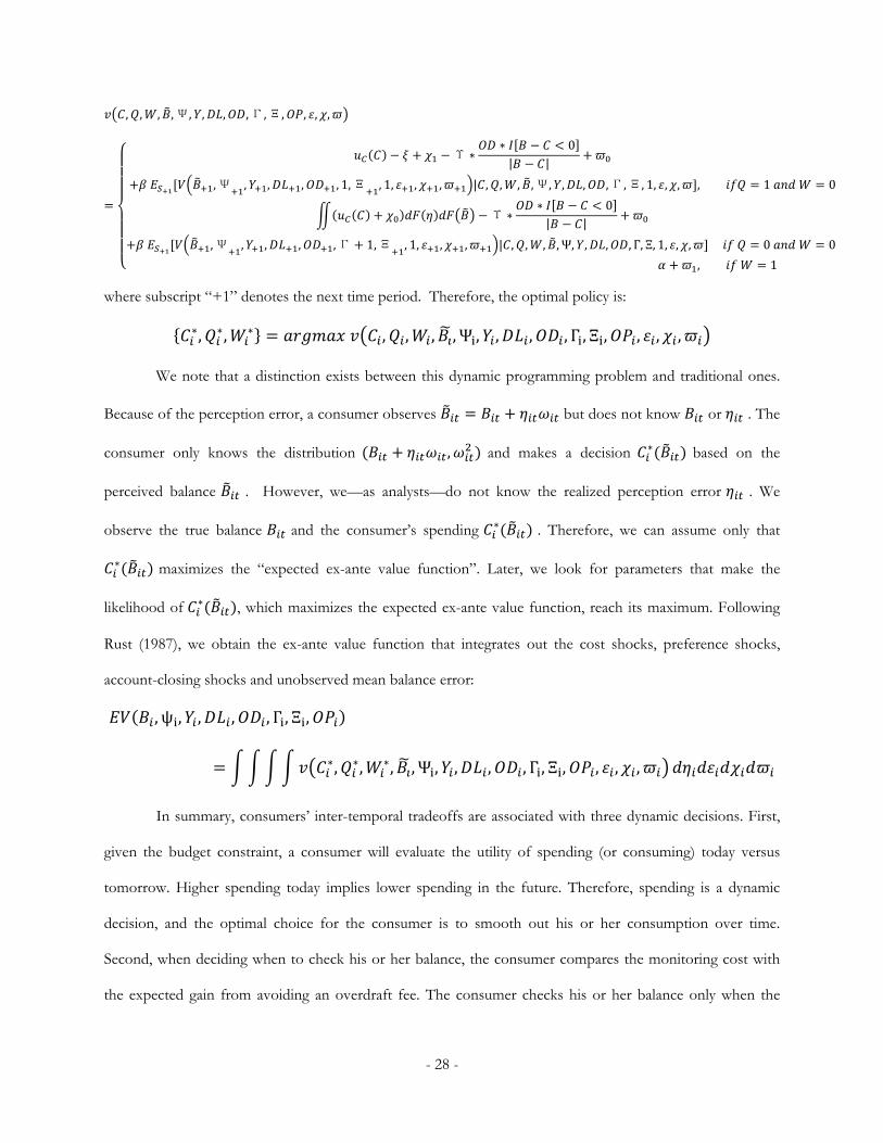
, , , ,Ψ, , , ,Γ,Ξ, , , ,

Υ ∗∗ 0| |

,Ψ , , , , 1,Ξ , 1, , , | , , , ,Ψ, , , ,Γ,Ξ, 1, , , , 1 0

Υ ∗∗ 0| |

,Ψ , , , ,Γ 1,Ξ , 1, , , | , , , , Ψ, , , , Γ, Ξ, 1, , , 0 0

, 1

where subscript “+1” denotes the next time period. Therefore, the optimal policy is:

∗, ∗, ∗ , , , , Ψ , , , , Γ , Ξ , , , ,

We note that a distinction exists between this dynamic programming problem and traditional ones.

Because of the perception error, a consumer observes but does not know or . The

consumer only knows the distribution , and makes a decision ∗ based on the

perceived balance . However, we—as analysts—do not know the realized perception error . We

observe the true balance and the consumer’s spending ∗ . Therefore, we can assume only that

∗ maximizes the “expected ex-ante value function”. Later, we look for parameters that make the

likelihood of ∗ , which maximizes the expected ex-ante value function, reach its maximum. Following

Rust (1987), we obtain the ex-ante value function that integrates out the cost shocks, preference shocks,

account-closing shocks and unobserved mean balance error:

, ψ , , , , Γ , Ξ ,

∗, ∗, ∗, , Ψ , , , , Γ , Ξ , , , ,

In summary, consumers’ inter-temporal tradeoffs are associated with three dynamic decisions. First,

given the budget constraint, a consumer will evaluate the utility of spending (or consuming) today versus

tomorrow. Higher spending today implies lower spending in the future. Therefore, spending is a dynamic

decision, and the optimal choice for the consumer is to smooth out his or her consumption over time.

Second, when deciding when to check his or her balance, the consumer compares the monitoring cost with

the expected gain from avoiding an overdraft fee. The consumer checks his or her balance only when the

- 29 -

expected overdraft fee is higher than the monitoring cost. Because the consumer’s balance perception error

might accumulate over time, the consumer’s overdraft probability also increases as more time elapses since

the last balance check. As a result, the consumer waits until the overdraft probability reaches a certain

threshold (when the expected overdraft fee equals the monitoring cost) before checking the balance. Finally,

the decision to close the account is an optimal stopping problem. The consumer will compare the total

discounted utility of keeping the account with the utility from the outside option to close the account. When

the consumer expects to incur many overdraft fees and the accompanying dissatisfaction, the consumer finds

it more attractive to take the outside option and close his or her account.

4.6 Heterogeneity

In our data, consumers exhibit different responses to their state conditions. For example, some

consumers have never checked their balance and frequently overdraw, while other consumers frequently

check their balance and rarely overdraw. We hypothesize that these differences result from their

heterogeneous discount factors and monitoring costs. Therefore, our model needs to account for unobserved

heterogeneity. We follow a hierarchical Bayesian framework (Rossi, McCulloch and Allenby 2005) and

incorporate heterogeneity into the model by assuming that all parameters, namely, (mean relative risk

averse coefficient), (discount factor), (standard deviation of the coefficient of risk aversion),

(monitoring cost), (sensitivity of the error variance to the time elapsed since the last balance check), Υ

(dissatisfaction sensitivity) and (mean value of the outside option), have a random coefficient specification.

The subscript i denotes the consumer, and the previous models are understood to be defined by the customer.

For each of these parameters ∈ , , , , , Υ , α , the prior distribution is defined as ∼ , .

The hyper-prior distribution is assumed to be diffuse.

- 30 -

5 Identification and Estimation

5.1 Identification

The unknown structural parameters in the model include , , , , , Υ , α , where is the

logarithm of the mean of the coefficient of risk aversion, is the discount factor, is the standard deviation

of the coefficient of risk aversion, is the monitoring cost, is the sensitivity of the balance error variance

to the time elapsed since the last balance check, Υ is the dissatisfaction sensitivity and is the mean value of

the outside option. We provide the rationale for the identification of each parameter.

We know from Rust (1987) that the discount factor cannot be separately identified from the static

utility parameter, which is the risk aversion coefficient in our case. The reason is that lowering tends to

increase consumption/spending, an effect that can also be achieved by lowering . Because we are more

interested in consumers’ time preference than their risk preference, we fix the risk aversion coefficient, which

allows us to identify the discount factor32. This practice is also used in Gopalakrishnan et al. (2014). Following

the latest research by Andersen et al. (2008), who jointly elicit risk and time preferences, we choose

0.74 for the coefficient of risk aversion33. After we fix , can be well identified by the sequences of

consumption (spending) within a pay period. A large discount factor (close to 1) implies a stable consumption

stream, while a small discount factor implies a downward-sloping consumption stream. Because a discount

factor is constrained above by 1, we take a logit transformation, namely,

, and estimate the

transformed parameter instead.

The standard deviation of the coefficient risk aversion is identified by the variation of

consumptions on the same day of the pay period but across different pay periods. Moreover, according to

the intertemporal tradeoff, the longer the consumer goes without checking his or her balance, the more likely

32 We also tried to fix the discount factor (at 0.9997) and estimate the coefficients of risk aversion. The posterior mean of the estimated coefficient of relative risk aversion is 0.72. Other structural parameter estimates are not significantly affected under this specification. Our results confirm that the coefficient of risk aversion and the discount factor are mathematically substitutes (Andersen et al. 2008). Estimation results with a fixed discount factor are available upon request. 33 We also tried other values for the coefficient of relative risk aversion . The estimated discount factor values change when we use different values of θ, but other structural parameter values remain the same. The policy simulation results are also robust to the use of different values of .

- 31 -

an overdraft is to occur because of a balance error. Therefore, the observed data pattern of higher overdraft

fees paid for a longer period after the balance is checked can inform the structural parameter .

Intuitively, the monitoring cost is identified by the expected overdraft payment amount. Recall

that the tradeoff regarding balance checking is that a consumer checks his or her balance only when is

smaller than the expected overdraft payment amount. In the data, we observe the balance-checking frequency.

By combining this with the calculated , we can compute the expected overdraft probability and then the

expected overdraft payment amount, which is the identified . Given , a consumer with few balance-

checking inquiries must have a higher balance-checking cost . The dissatisfaction sensitivity parameter Υ

can be identified by the data pattern where consumers’ account closure probability varies with the ratio of the

overdraft fee to the overdraft transaction amount, as shown in our exploratory data analysis (§ 3.2.3). Lastly,

the mean value of the outside option can be identified by the average account closing probability.

Note that aside from these structural parameters, another set of parameters governs the transition

process. These parameters can be identified prior to the structural estimation from the observed state

variables in our data. The set includes , , , .

In summary, the structural parameters to be estimated include , , , , Υ , .

5.2 Likelihood

The full likelihood function is

, , | | , , ,

where , , , , , Γ , Ξ , . Because the likelihood for the optimal choice and that

for the state transition process are additively separable when we apply a log transformation to the likelihood

function, we can first estimate the state transition process from the data and then maximize the likelihood for

the optimal choice. The likelihood function for the optimal choice is

- 32 -

, , | , , |

| | |

where | is estimated from the normal kernel density estimator (explained in the next section) and

| and | follow the standard logit model given the choice-specific value function.

Using the logit specification, we can write:

Pr 1|, 1, ,

∑ , , ,

Pr 1|, , 1,

∑ , , ,

5.3 Initial Conditions

For each consumer i, we simulate the model for 60 initial periods to derive the initial state variables.

Then we proceed to construct the likelihood increment for consumer i.

5.4 Estimation Using the Imai, Jain and Ching (2009) Algorithm

We aim to estimate our infinite horizon dynamic structural model on a large dataset, and we want to

obtain individual responses so that we can recommend targeted marketing strategies. We investigate several

estimation methods, including the nested fixed point algorithm (Rust 1987), the conditional choice probability

estimation (Arcidiacono and Miller 2011) and the Bayesian estimation method developed in Imai, Jain and

Ching (2009) (IJC). We adopt the IJC method for the following reasons. First, the hierarchical Bayes

framework fits our goal of obtaining heterogeneous parameters. Second, we apply the model to a large dataset,

so the estimation is computationally challenging. Fortunately, Bayesian MCMC can be combined with a

parallel computing technique to reduce the computational burden. Third, IJC is the state-of-the-art Bayesian

estimation algorithm for infinite horizon dynamic programming models. The IJC algorithm provides two

additional benefits in tackling the computational challenges. One is that it alleviates the computational burden

- 33 -

by evaluating the value function only once in each epoch. Essentially, the algorithm solves the value function

and estimates the structural parameters simultaneously. Thus, the computational burden of a dynamic

problem is reduced by an order of magnitude with computational costs similar to a static model. The other is

that the method reduces the curse of dimensionality by allowing state space grid points to vary between

estimation iterations.

Given the massive size of our dataset, a traditional MCMC estimation may take a prohibitively long

time, because most methods must perform O(N) operations for N data points. A natural way to reduce the

computation time is to run the chain in parallel. Past methods of parallel MCMC duplicate the data on

multiple machines and cannot reduce the time of burn-in. We instead use a new technique developed by

Neiswanger, Wang and Xing (2014) to address this problem. The key idea of this algorithm is that the data

can be distributed into multiple machines and the IJC estimation can be performed in parallel. Once we

obtain the posterior Markov Chains from each machine, we can algorithmically combine these individual

chains to obtain the posterior chain of the whole sample.

5.4.1 Modified IJC

Our model involves a continuous choice variable, spending. Therefore, we modify the IJC

algorithm34 to obtain the choice probability through kernel density estimation. We provide a sketch of our

estimation procedure and refer the reader to Appendix A2 for more details. The whole parameter space is

divided into two sets ( Ω Ω , Ω ), where the first one contains the set of hyper-parameters ( Ω

, , , , , , , , , , , ) and the second set contains the set of heterogeneous

parameters ( Ω , , , , Υ , ). We allow all the heterogeneous parameters (represented by )

to follow a normal distribution with mean and standard deviation for the parameters. Let the observed

choices be , , , where ≡ , ∀ , ≡ , ∀ and ≡

, ∀ .

Each MCMC iteration consists of two blocks: 34 The IJC method is designed for dynamic discrete choice problems. Zhou (2012) also applied it to a continuous choice problem.

- 34 -

(i) Draw Ω ; that is, draw ∼ | , Ω and ∼ | , Ω

( ∈ , , , , Υ, α , the parameters that capture the distribution of for the population), where and

are the conditional posterior distributions.

(ii) Draw Ω ; that is, draw individual parameters ∼ | , Ω by the Metropolis-Hastings (M-H)

algorithm.

5.4.2 Parallel Computing Following Neiswanger, Wang and Xing (2014)

We adopt the parallel computing algorithm by Neiswanger, Wang and Xing (2014) to estimate our

model with data for more than 500,000 consumers. The logic behind this algorithm is that the full likelihood

function is the product of the individual likelihoods:

| ∝ | |

Therefore, we can partition the data onto multiple machines and then perform MCMC sampling on each

machine by using only the subset of data on that machine (in parallel, without any communication). Finally,

we can combine the subposterior samples to algorithmically construct samples from the full-data posterior.

Our procedure is outlined below (for additional details, see Appendix A3):

(1) Partition data into M subsets , . . . , .

(2) For 1, . . . , (in parallel):

(a) Sample from the subposterior , where | ∝ | .

(3) Combine the subposterior samples to produce samples from an estimate of the subposterior density

product … , which is proportional to the full-data posterior, i.e., … ∝ | .

Given samples from a subposterior , we can write the kernel density estimator as

,

1 1 || ||

- 35 -

12 | |

12

1| ,

where we have used a Gaussian kernel with bandwidth parameter and where is the dimensionality. After

we have obtained the kernel density estimator for M subposteriors, we define our nonparametric

density product estimator for the full posterior as

⋯

⋯

1⋯ | ,

∝ ⋯ | ∙, | ∙,

⋯ ∙ | ∙,

This estimate is the probability density function (pdf) of a mixture of T^M Gaussians with

unnormalized mixture weights ∙ Here, we use ⋅ , … , to denote the set of indices for the M

samples , … , (each from one machine) associated with a given mixture component, and we let

∙ | ∙,

∙1

- 36 -

Given the hierarchical Bayes framework, after the posterior distribution of the population parameter is

obtained, we use the M-H algorithm once more to obtain the individual parameters (see the details in

Appendix A2, Step 4).

6 Results

6.1 Model Comparison

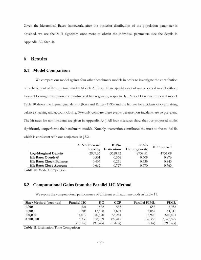
We compare our model against four other benchmark models in order to investigate the contribution

of each element of the structural model. Models A, B, and C are special cases of our proposed model without

forward looking, inattention and unobserved heterogeneity, respectively. Model D is our proposed model.

Table 10 shows the log-marginal density (Kass and Raftery 1995) and the hit rate for incidents of overdrafting,

balance checking and account closing. (We only compare these events because non-incidents are so prevalent.

The hit rates for non-incidents are given in Appendix A4.) All four measures show that our proposed model

significantly outperforms the benchmark models. Notably, inattention contributes the most to the model fit,

which is consistent with our conjecture in §3.2.

A: No Forward

LookingB: No

InattentionC: No

Heterogeneity D: Proposed

Log-Marginal Density -2937.66 -3628.72 -2759.51 -1751.08Hit Rate: Overdraft 0.501 0.356 0.509 0.876Hit Rate: Check Balance 0.407 0.231 0.639 0.843Hit Rate: Close Account 0.662 0.727 0.670 0.763

Table 10. Model Comparison

6.2 Computational Gains from the Parallel IJC Method

We report the computational performance of different estimation methods in Table 11.

Size\Method (seconds) Parallel IJC IJC CCP Parallel FIML FIML1,000 521 1582 533 658 5,03210,000 3,205 12,588 4,694 4,887 54,311100,000 4,072 140,870 55,281 15,920 640,403>500,000 5,339 788,389 399,417 32,388 3,372,895 (1.5 hr) (9 days) (5 days) (9 hr) (39 days)

Table 11. Estimation Time Comparison

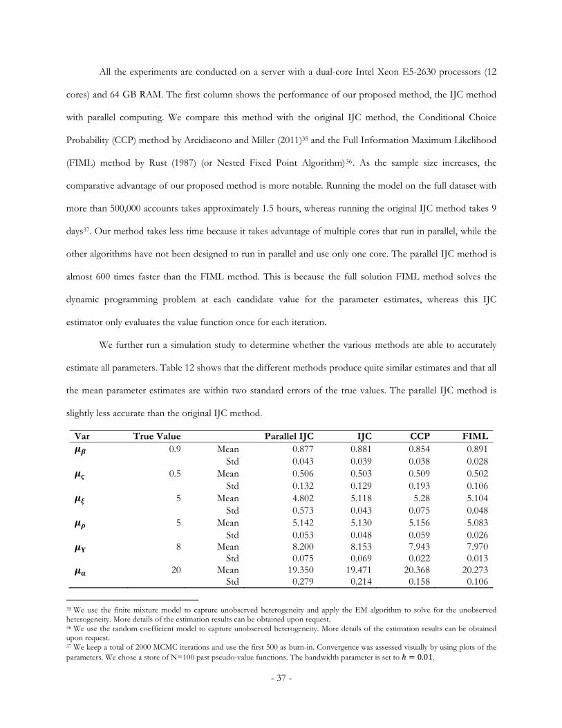
- 37 -

All the experiments are conducted on a server with a dual-core Intel Xeon E5-2630 processors (12

cores) and 64 GB RAM. The first column shows the performance of our proposed method, the IJC method

with parallel computing. We compare this method with the original IJC method, the Conditional Choice

Probability (CCP) method by Arcidiacono and Miller (2011)35 and the Full Information Maximum Likelihood

(FIML) method by Rust (1987) (or Nested Fixed Point Algorithm)36. As the sample size increases, the

comparative advantage of our proposed method is more notable. Running the model on the full dataset with

more than 500,000 accounts takes approximately 1.5 hours, whereas running the original IJC method takes 9

days37. Our method takes less time because it takes advantage of multiple cores that run in parallel, while the

other algorithms have not been designed to run in parallel and use only one core. The parallel IJC method is

almost 600 times faster than the FIML method. This is because the full solution FIML method solves the

dynamic programming problem at each candidate value for the parameter estimates, whereas this IJC

estimator only evaluates the value function once for each iteration.

We further run a simulation study to determine whether the various methods are able to accurately

estimate all parameters. Table 12 shows that the different methods produce quite similar estimates and that all

the mean parameter estimates are within two standard errors of the true values. The parallel IJC method is

slightly less accurate than the original IJC method.

Var True Value Parallel IJC IJC CCP FIML 0.9 Mean 0.877 0.881 0.854 0.891

Std 0.043 0.039 0.038 0.028 0.5 Mean 0.506 0.503 0.509 0.502

Std 0.132 0.129 0.193 0.106 5 Mean 4.802 5.118 5.28 5.104

Std 0.573 0.043 0.075 0.048 5 Mean 5.142 5.130 5.156 5.083

Std 0.053 0.048 0.059 0.026 8 Mean 8.200 8.153 7.943 7.970

Std 0.075 0.069 0.022 0.013 20 Mean 19.350 19.471 20.368 20.273

Std 0.279 0.214 0.158 0.106

35 We use the finite mixture model to capture unobserved heterogeneity and apply the EM algorithm to solve for the unobserved heterogeneity. More details of the estimation results can be obtained upon request. 36 We use the random coefficient model to capture unobserved heterogeneity. More details of the estimation results can be obtained upon request. 37 We keep a total of 2000 MCMC iterations and use the first 500 as burn-in. Convergence was assessed visually by using plots of the parameters. We chose a store of N=100 past pseudo-value functions. The bandwidth parameter is set to 0.01.

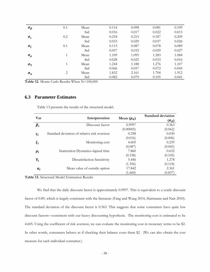
- 38 -

0.1 Mean 0.114 0.098 0.081 0.109 Std 0.016 0.017 0.022 0.013

0.2 Mean 0.218 0.215 0.187 0.209 Std 0.033 0.029 0.037 0.026

0.1 Mean 0.113 0.087 0.078 0.089 Std 0.057 0.032 0.029 0.027

1 Mean 1.109 1.095 1.283 1.084 Std 0.028 0.025 0.033 0.016

1 Mean 1.244 1.188 1.276 1.107 Std 0.066 0.057 0.072 0.045

2 Mean 1.832 2.161 1.704 1.912 Std 0.082 0.070 0.105 0.041

Table 12. Monte Carlo Results When N=100,000

6.3 Parameter Estimates

Table 13 presents the results of the structural model.

Var Interpretation Mean ( )Standard deviation

( ) Discount factor 0.9997 0.363

(0.00005) (0.062) Standard deviation of relative risk aversion 0.258 0.030

(0.016) (0.006) Monitoring cost 4.605 0.259

(0.087) (0.043) Inattention Dynamics–lapsed time 7.860 0.652

(0.338) (0.105) Dissatisfaction Sensitivity 5.446 1.278

(1.356) (0.118) Mean value of outside option 17.842 2.361

(1.660) (0.837)Table 13. Structural Model Estimation Results

We find that the daily discount factor is approximately 0.9997. This is equivalent to a yearly discount

factor of 0.89, which is largely consistent with the literature (Fang and Wang 2014, Hartmann and Nair 2010).

The standard deviation of the discount factor is 0.363. This suggests that some consumers have quite low

discount factors—consistent with our heavy discounting hypothesis. The monitoring cost is estimated to be

4.605. Using the coefficient of risk aversion, we can evaluate the monitoring cost in monetary terms to be $2.

In other words, consumers behave as if checking their balance costs them $2. (We can also obtain the cost

measure for each individual consumer.)

- 39 -

The variance of the balance perception error increases with the time elapsed since the last balance

check and with the mean balance level. Notably, the variance in the balance perception error is quite large. If

we take the average number of days to check the balance from the data, which is 9, then the standard

deviation is 7.860*9=70.74. This suggests that the balance perception error has a diffuse distribution.

The estimated dissatisfaction sensitivity parameters confirm our hypothesis that consumers can be

strongly affected by overdraft fees and close their account due to dissatisfaction. If we consider an average

overdraft transaction amount of $33, then the relative magnitude of the effect of dissatisfaction is comparable

to $171. This suggests that unless the bank would like to offer $171 in compensation to consumers,

dissatisfied consumers will close their current account and choose the outside option. Moreover, consistent

with our exploratory data analysis (see Figure 5), the dissatisfaction sensitivity is stronger for light overdrafters

(whose average is 5.911) than for heavy overdrafters (whose average is 3.387). Keeping the average overdraft

transaction amount fixed, a 1% increase in the overdraft fee can increase the closing probability by 0.12%.

7 Counterfactual Studies of Alternative Overdrafting Policies

Our structural model allows us to examine counterfactual studies that consider the effect of changing

the pricing structure on consumers’ spending patterns and, more importantly, their overdrafting behavior. We

test the effect of three alternative pricing schemes, namely, a reduced per-item flat fee, a percentage fee, and a

quantity premium. We provide the results in Table 14Error! Reference source not found.. We make two

assumptions for all these simulations. One is fungibility, i.e., a consumer’s reaction depends only on the fee

amount rather than the fee structure. If two different fee structures result in the same fee amount, then

consumers should respond in the same fashion. The other is the universal dissatisfaction effect. We assume

that consumers’ dissatisfaction effect is proportional to the ratio of the overdraft fee to the transaction

amount, despite the fee structure. It is possible that consumers will be less dissatisfied with alternative pricing

schemes, such as a percentage fee, because they may be perceived as more fair (Bolton, Warlop and Alba

2003). However, we argue that rational consumers discover the commonality between different pricing

strategies and react to only the essential factor (implicit price) that triggers dissatisfaction. 

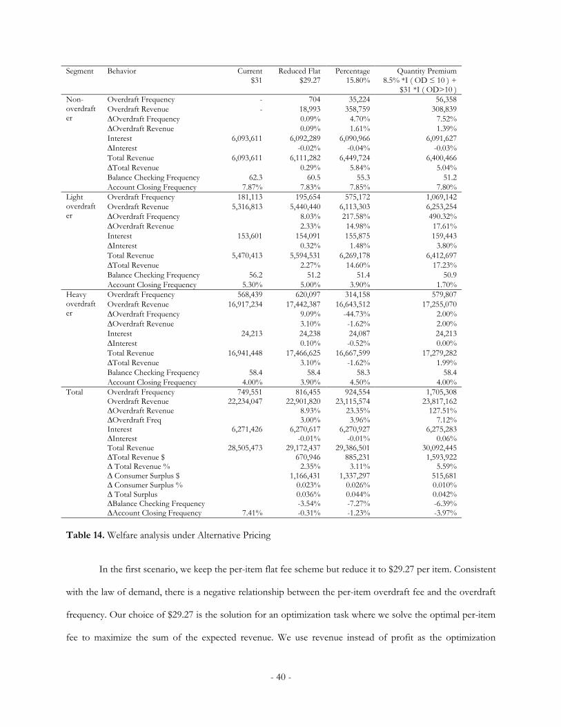
- 40 -

Segment Behavior Current Reduced Flat Percentage Quantity Premium $31 $29.27 15.80% 8.5% *I ( OD ≤ 10 ) +

$31 *I ( OD>10 )Non-overdrafter

Overdraft Frequency - 704 35,224 56,358 Overdraft Revenue - 18,993 358,759 308,839 ∆Overdraft Frequency 0.09% 4.70% 7.52%∆Overdraft Revenue 0.09% 1.61% 1.39%Interest 6,093,611 6,092,289 6,090,966 6,091,627 ∆Interest -0.02% -0.04% -0.03%Total Revenue 6,093,611 6,111,282 6,449,724 6,400,466 ∆Total Revenue 0.29% 5.84% 5.04%Balance Checking Frequency 62.3 60.5 55.3 51.2Account Closing Frequency 7.87% 7.83% 7.85% 7.80%

Light overdrafter

Overdraft Frequency 181,113 195,654 575,172 1,069,142 Overdraft Revenue 5,316,813 5,440,440 6,113,303 6,253,254 ∆Overdraft Frequency 8.03% 217.58% 490.32%∆Overdraft Revenue 2.33% 14.98% 17.61%Interest 153,601 154,091 155,875 159,443 ∆Interest 0.32% 1.48% 3.80%Total Revenue 5,470,413 5,594,531 6,269,178 6,412,697 ∆Total Revenue 2.27% 14.60% 17.23%Balance Checking Frequency 56.2 51.2 51.4 50.9Account Closing Frequency 5.30% 5.00% 3.90% 1.70%

Heavy overdrafter

Overdraft Frequency 568,439 620,097 314,158 579,807 Overdraft Revenue 16,917,234 17,442,387 16,643,512 17,255,070∆Overdraft Frequency 9.09% -44.73% 2.00%∆Overdraft Revenue 3.10% -1.62% 2.00%Interest 24,213 24,238 24,087 24,213 ∆Interest 0.10% -0.52% 0.00%Total Revenue 16,941,448 17,466,625 16,667,599 17,279,282 ∆Total Revenue 3.10% -1.62% 1.99%Balance Checking Frequency 58.4 58.4 58.3 58.4Account Closing Frequency 4.00% 3.90% 4.50% 4.00%

Total Overdraft Frequency 749,551 816,455 924,554 1,705,308 Overdraft Revenue 22,234,047 22,901,820 23,115,574 23,817,162 ∆Overdraft Revenue 8.93% 23.35% 127.51%∆Overdraft Freq 3.00% 3.96% 7.12%Interest 6,271,426 6,270,617 6,270,927 6,275,283 ∆Interest -0.01% -0.01% 0.06%Total Revenue 28,505,473 29,172,437 29,386,501 30,092,445 ∆Total Revenue $ 670,946 885,231 1,593,922 ∆ Total Revenue % 2.35% 3.11% 5.59%∆ Consumer Surplus $ 1,166,431 1,337,297 515,681 ∆ Consumer Surplus % 0.023% 0.026% 0.010%∆ Total Surplus 0.036% 0.044% 0.042%∆Balance Checking Frequency -3.54% -7.27% -6.39%∆Account Closing Frequency 7.41% -0.31% -1.23% -3.97%

Table 14. Welfare analysis under Alternative Pricing

In the first scenario, we keep the per-item flat fee scheme but reduce it to $29.27 per item. Consistent

with the law of demand, there is a negative relationship between the per-item overdraft fee and the overdraft

frequency. Our choice of $29.27 is the solution for an optimization task where we solve the optimal per-item

fee to maximize the sum of the expected revenue. We use revenue instead of profit as the optimization

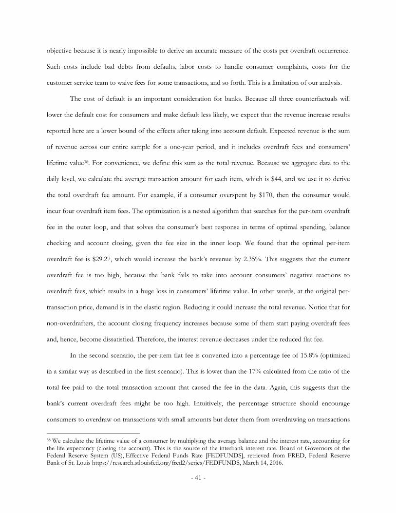
- 41 -

objective because it is nearly impossible to derive an accurate measure of the costs per overdraft occurrence.

Such costs include bad debts from defaults, labor costs to handle consumer complaints, costs for the

customer service team to waive fees for some transactions, and so forth. This is a limitation of our analysis.

The cost of default is an important consideration for banks. Because all three counterfactuals will

lower the default cost for consumers and make default less likely, we expect that the revenue increase results

reported here are a lower bound of the effects after taking into account default. Expected revenue is the sum

of revenue across our entire sample for a one-year period, and it includes overdraft fees and consumers’

lifetime value38. For convenience, we define this sum as the total revenue. Because we aggregate data to the

daily level, we calculate the average transaction amount for each item, which is $44, and we use it to derive

the total overdraft fee amount. For example, if a consumer overspent by $170, then the consumer would

incur four overdraft item fees. The optimization is a nested algorithm that searches for the per-item overdraft

fee in the outer loop, and that solves the consumer’s best response in terms of optimal spending, balance

checking and account closing, given the fee size in the inner loop. We found that the optimal per-item

overdraft fee is $29.27, which would increase the bank’s revenue by 2.35%. This suggests that the current

overdraft fee is too high, because the bank fails to take into account consumers’ negative reactions to

overdraft fees, which results in a huge loss in consumers’ lifetime value. In other words, at the original per-

transaction price, demand is in the elastic region. Reducing it could increase the total revenue. Notice that for

non-overdrafters, the account closing frequency increases because some of them start paying overdraft fees

and, hence, become dissatisfied. Therefore, the interest revenue decreases under the reduced flat fee.

In the second scenario, the per-item flat fee is converted into a percentage fee of 15.8% (optimized

in a similar way as described in the first scenario). This is lower than the 17% calculated from the ratio of the

total fee paid to the total transaction amount that caused the fee in the data. Again, this suggests that the

bank’s current overdraft fees might be too high. Intuitively, the percentage structure should encourage

consumers to overdraw on transactions with small amounts but deter them from overdrawing on transactions

38 We calculate the lifetime value of a consumer by multiplying the average balance and the interest rate, accounting for the life expectancy (closing the account). This is the source of the interbank interest rate. Board of Governors of the Federal Reserve System (US), Effective Federal Funds Rate [FEDFUNDS], retrieved from FRED, Federal Reserve Bank of St. Louis https://research.stlouisfed.org/fred2/series/FEDFUNDS, March 14, 2016.

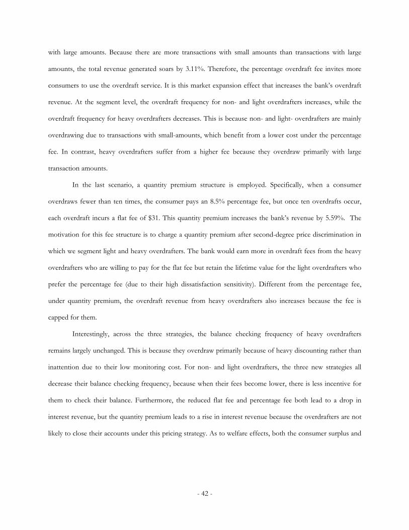
- 42 -

with large amounts. Because there are more transactions with small amounts than transactions with large

amounts, the total revenue generated soars by 3.11%. Therefore, the percentage overdraft fee invites more

consumers to use the overdraft service. It is this market expansion effect that increases the bank’s overdraft

revenue. At the segment level, the overdraft frequency for non- and light overdrafters increases, while the

overdraft frequency for heavy overdrafters decreases. This is because non- and light- overdrafters are mainly

overdrawing due to transactions with small-amounts, which benefit from a lower cost under the percentage

fee. In contrast, heavy overdrafters suffer from a higher fee because they overdraw primarily with large

transaction amounts.

In the last scenario, a quantity premium structure is employed. Specifically, when a consumer

overdraws fewer than ten times, the consumer pays an 8.5% percentage fee, but once ten overdrafts occur,

each overdraft incurs a flat fee of $31. This quantity premium increases the bank’s revenue by 5.59%. The

motivation for this fee structure is to charge a quantity premium after second-degree price discrimination in

which we segment light and heavy overdrafters. The bank would earn more in overdraft fees from the heavy

overdrafters who are willing to pay for the flat fee but retain the lifetime value for the light overdrafters who

prefer the percentage fee (due to their high dissatisfaction sensitivity). Different from the percentage fee,

under quantity premium, the overdraft revenue from heavy overdrafters also increases because the fee is

capped for them.

Interestingly, across the three strategies, the balance checking frequency of heavy overdrafters

remains largely unchanged. This is because they overdraw primarily because of heavy discounting rather than

inattention due to their low monitoring cost. For non- and light overdrafters, the three new strategies all

decrease their balance checking frequency, because when their fees become lower, there is less incentive for

them to check their balance. Furthermore, the reduced flat fee and percentage fee both lead to a drop in

interest revenue, but the quantity premium leads to a rise in interest revenue because the overdrafters are not

likely to close their accounts under this pricing strategy. As to welfare effects, both the consumer surplus and

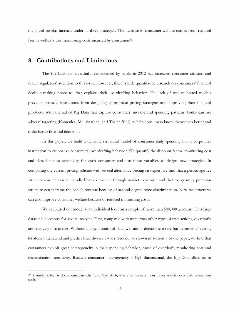
- 43 -

the social surplus increase under all three strategies. The increase in consumer welfare comes from reduced

fees as well as lower monitoring costs incurred by consumers39.

8 Contributions and Limitations

The $32 billion in overdraft fees assessed by banks in 2012 has increased consumer attrition and

drawn regulators’ attention to this issue. However, there is little quantitative research on consumers’ financial

decision-making processes that explains their overdrafting behavior. The lack of well-calibrated models

prevents financial institutions from designing appropriate pricing strategies and improving their financial

products. With the aid of Big Data that capture consumers’ income and spending patterns, banks can use

adverse targeting (Kamenica, Mullainathan, and Thaler 2011) to help consumers know themselves better and

make better financial decisions.

In this paper, we build a dynamic structural model of consumer daily spending that incorporates

inattention to rationalize consumers’ overdrafting behavior. We quantify the discount factor, monitoring cost

and dissatisfaction sensitivity for each consumer and use these variables to design new strategies. In

comparing the current pricing scheme with several alternative pricing strategies, we find that a percentage fee

structure can increase the studied bank’s revenue through market expansion and that the quantity premium

structure can increase the bank’s revenue because of second-degree price discrimination. New fee structures

can also improve consumer welfare because of reduced monitoring costs.

We calibrated our model at an individual level on a sample of more than 500,000 accounts. This large

dataset is necessary for several reasons. First, compared with numerous other types of transactions, overdrafts

are relatively rare events. Without a large amount of data, we cannot detect these rare but detrimental events,

let alone understand and predict their diverse causes. Second, as shown in section 3 of the paper, we find that

consumers exhibit great heterogeneity in their spending behavior, cause of overdraft, monitoring cost and

dissatisfaction sensitivity. Because consumer heterogeneity is high-dimensional, the Big Data allow us to

39 A similar effect is documented in Chen and Yao 2016, where consumers incur lower search costs with refinement tools.

- 44 -

capture this rich consumer heterogeneity in a much more refined fashion. Third, a selected subset might

suffer from sampling error or sample bias. Because consumer behaviors and characteristics are high-

dimensional, it is difficult to collect an accurate, random and representative sample. To illustrate the potential

sampling error, we performed the same analysis on a 10% subset of the data. The predicted revenue in the

counterfactual of the quantity premium strategy is 6%, or 0.3 million dollars less than the value obtained from

results using the entire dataset. In other words, the sampling error might lead to an incorrect strategy and a

significant loss to the bank. Therefore, we argue that, given the sizable sampling error, if the computational

burden of estimating a dynamic structural model on a large dataset is minimal, as demonstrated by our parallel

IJC algorithm, using the full dataset is preferred.

To estimate a complicated structural model with Big Data, we adopt parallel computing techniques in

combination with the Bayesian estimation algorithm developed by Imai, Jain and Ching (2009). This new

method significantly reduces the computation burden, and it could be used by other researchers and

marketers who would like to use structural models to solve real-world large-scale problems. Although we

apply it to the overdraft context, the model framework can be generalized to analyze other marketing

problems in which consumers have similar dynamic budget allocation decisions (e.g., utility accounts and

mobile phones).

Several limitations of the current study call for future work. First, we do not observe consumers’

existing alert settings. Some consumers may have already received alerts to help them make financial decisions.

This might cause an overestimation of the monitoring cost and an underestimation of the inattention

sensitivity to lapsed time. But given the prevalence of overdrafts, we conjecture that many consumers are not

using alerts. And because our counterfactual only alters the pricing strategies, we cannot think of any reason

that our welfare analysis results can be different after accounting for alerts. Second, we do not have data on

consumers’ decision to opt-in for overdraft protection by ATM/POS transactions. We only know that if

ATM/POS transactions caused an overdraft, then the consumer must have opted-in. If no such transactions

occurred, we do not know the consumer’s opt-in status. Had we known this information, we could have

provided an informative prior within our Bayesian model, as consumers who have opted-in probably have

- 45 -

stronger needs for short-term liquidity owing to fluctuations in the size and arrival time of their income and

spending. Third, we lack precise data on the bank’s cost structure, and while we can make predictions about

its revenue, we cannot predict its profits. Finally, we only model consumers’ non-preauthorized spending in

their checking account. In reality, consumers usually have multiple accounts, such as savings, credit cards and

loans, with multiple financial institutions. A model that captures consumers’ decisions across all accounts for

both short-term and long-term finances would provide a more complete picture of consumers’ financial

management capabilities and resources so that the bank can design more-customized products.

- 46 -

References

Andersen, S., Harrison, G. W., Lau, M. I., & Rutström, E. E. (2008). Eliciting risk and time preferences. Econometrica, 76(3), 583-618.

Arcidiacono, P., & Miller, R. A. (2011). Conditional choice probability estimation of dynamic discrete choice models with unobserved heterogeneity. Econometrica, 79(6), 1823-1867.

Arrow, K. J. 1963. Liquidity preference. Lecture VI in Lecture Notes for Economics 285, The Economics of Uncertainty, pp. 33-53, undated, Stanford University.

Bellman, R. 1957. Dynamic Programming, Princeton, NJ: Princeton University Press.

Bolton, R. N. (1998). A dynamic model of the duration of the customer’s relationship with a continuous service provider: the role of satisfaction. Marketing science, 17(1), 45-65.

Bolton, L. E., Warlop, L., & Alba, J. W. (2003). Consumer perceptions of price (un) fairness. Journal of consumer research, 29(4), 474-491.

Chetty, R., Looney, A., & Kroft, K. (2009). Salience and taxation: Theory and evidence. American Economic Review, 99(4), 1145-1177.

DellaVigna, S. (2009). Psychology and Economics: Evidence from the Field.Journal of Economic Literature, 47(2), 315-372.Einav, L., & Levin, J. D. (2014). The data revolution and economic analysis. Innovation Policy and the Economy, forthcoming.

Evans, D., Litan, R., & Schmalensee, R. (2011). Economic Analysis of the Effects of the Federal Reserve Board’s Proposed Debit Card Interchange Fee Regulations on Consumers and Small Businesses. Available at SSRN 1769887.

Fang, H., & Silverman, D. (2009). Time-inconsistency and welfare program participation: Evidence from the nlsy. International Economic Review, 50(4), 1043-1077.

Fang, H., & Yang W. (2014). Estimating Dynamic Discrete Choice Models with Hyperbolic Discounting, with an Application to Mammography Decisions. International Economic Review, forthcoming.

Fishman, M. J., & Hagerty, K. M. (2003). Mandatory versus voluntary disclosure in markets with informed and uninformed customers. Journal of Law, Economics, and Organization, 19(1), 45-63.

Fiske, Susan T. and Shelley E. Taylor (1991), Social Cognition, 2d ed., New York: McGraw-Hill.

Friend, I. and M. Blume (1975). “The Demand for Risky Assets,” American Economic Review, 65 (December), pp. 900-22.

Gabaix, X., & Laibson, D. (2006). Shrouded attributes, consumer myopia, and information suppression in competitive markets. The Quarterly Journal of Economics, 121(2), 505-540.

Gopalakrishnan, A., Iyengar, R., & Meyer, R. J. (2014). Consumer dynamic usage allocation and learning under multi-part tariffs: theory and empirical evidence. Working paper, Wharton School, University of Pennsylvania.

Grubb, M. D. (2014). Consumer inattention and bill-shock regulation. The Review of Economic Studies, rdu024.

Grubb, M. D., & Osborne, M. (2015). Cellular Service Demand: Biased Beliefs, Learning, and Bill Shock. American Economic Review, 105(1), 234-271.

Hartmann, W. R., Harikesh S. N. 2010. Retail competition and the dynamics of demand for tied goods. Marketing Science, 29(2), 366–386.

- 47 -

Haselhuhn, M. P., Pope, D. G., Schweitzer, M. E., & Fishman, P. (2012). The impact of personal experience on behavior: Evidence from video-rental fines. Management Science, 58(1), 52-61.

Hirshleifer, D., & Hong Teoh, S. (2003). Herd behaviour and cascading in capital markets: A review and synthesis. European Financial Management, 9(1), 25-66.

Imai, S., Jain, N., & Ching, A. (2009). Bayesian estimation of dynamic discrete choice models. Econometrica, 77(6), 1865-1899.

Jiang, L. (2012). The welfare effects of "bill shock" regulation in mobile telecommunication markets. Working Paper, University of British Columbia.

Kahneman, D., J. Knetsch, and R. Thaler (1990). Experimental Tests of the Endowment Effect and the Coase Theorem. Journal of Political Economy, 98(6), 1325–1348.

Kahneman, D., & Tversky, A. (1979). Prospect theory: An analysis of decision under risk. Econometrica: Journal of the Econometric Society, 263-291.

Kamenica, E., Mullainathan, S., & Thaler, R. (2011). Helping consumers know themselves. The American Economic Review, 101(3), 417-422.

Karlan, D., McConnell, M., Mullainathan, S., & Zinman, J. (2010). Getting to the top of mind: How reminders increase saving (No. w16205). National Bureau of Economic Research.

Kass, R., and A. Raftery. (1995). Bayes Factors. Journal of the American Statistical Association 90 (430): 773-95.

Keaveney, S. M. (1995). Customer switching behavior in service industries: an exploratory study. The Journal of Marketing, 71-82.

Magnac, T., & Thesmar, D. (2002). Identifying dynamic discrete decision processes. Econometrica, 70(2), 801-816.

Matzler, K., Würtele, A., & Renzl, B. (2006). Dimensions of price satisfaction: a study in the retail banking industry. International Journal of Bank Marketing, 24(4), 216-231.

Mehta, N., Rajiv, S., & Srinivasan, K. (2003). Price uncertainty and consumer search: A structural model of consideration set formation. Marketing science, 22(1), 58-84.

Merton, R. (1992). Continuous Time Finance, (Cambridge: Blackwell Publishing Co.).

Monroe, Kent B. (1990), Pricing: Making Profitable Decision, New York: McGraw-Hill.

Neiswanger, W., Wang, C., & Xing, E. (2014). Asymptotically exact, embarrassingly parallel MCMC. Proceedings of the 30th International Conference on Conference on Uncertainty in Artificial Intelligence.

Nwokoye, N. G. (1975). Subjective judgments of price: The effects of price parameters on adaptation levels. In Proceedings of Fall Conference. Chicago: American Marketing Association.

Peng, L., & Xiong, W. (2006). Investor attention, overconfidence and category learning. Journal of Financial Economics, 80(3), 563-602.

Pope, D. G. (2009). Reacting to rankings: Evidence from “America’s Best Hospitals”. Journal of Health Economics, 28(6), 1154-1165.

Reis, R. (2006). Inattentive producers. The Review of Economic Studies,73(3), 793-821.

Rossi, Peter E., Allenby, G. M., & McCulloch, R. E. (2005). Bayesian statistics and marketing. J. Wiley & Sons.

Rust, J. (1987). Optimal replacement of GMC bus engines: An empirical model of Harold Zurcher. Econometrica: Journal of the Econometric Society, 999-1033.

- 48 -

Stango, V., & Zinman, J. (2014). Limited and varying consumer attention evidence from shocks to the salience of bank overdraft fees. Review of Financial Studies, hhu008.

Tversky, Amos and Daniel Kahneman (1973). Availability: A Heuristic for Judging Frequency and Probable Cause. Cognitive Psychology, 5 (September), 207–232.

Yao, S., Mela, C. F., Chiang, J., & Chen, Y. (2012). Determining consumers’ discount rates with field studies. Journal of Marketing Research, 49(6), 822-841.

Zhou, Y. (2012). Failure to Launch in Two-Sided Markets: A Study of the US Video Game Market. Working paper, SUNY at Stony Brook.

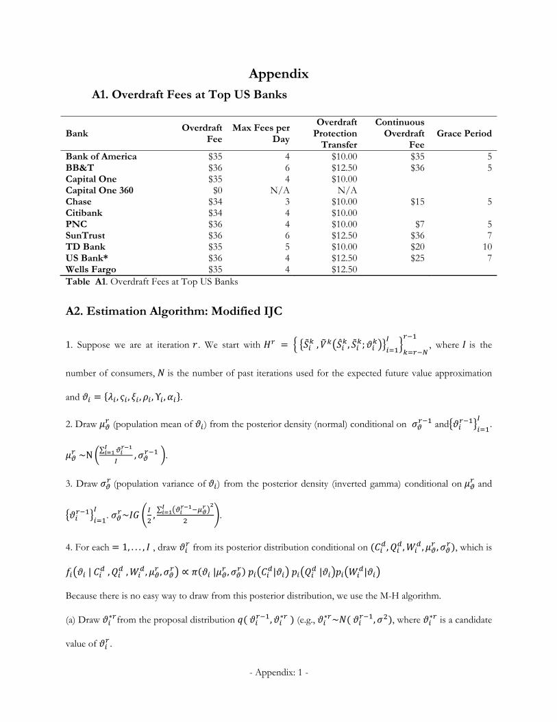
- Appendix: 1 -

Appendix

A1. Overdraft Fees at Top US Banks

Bank Overdraft

Fee Max Fees per

Day

Overdraft Protection

Transfer

Continuous Overdraft

Fee Grace Period

Bank of America $35 4 $10.00 $35 5BB&T $36 6 $12.50 $36 5Capital One $35 4 $10.00 Capital One 360 $0 N/A N/A Chase $34 3 $10.00 $15 5Citibank $34 4 $10.00 PNC $36 4 $10.00 $7 5SunTrust $36 6 $12.50 $36 7TD Bank $35 5 $10.00 $20 10US Bank* $36 4 $12.50 $25 7Wells Fargo $35 4 $12.50 Table A1. Overdraft Fees at Top US Banks

A2. Estimation Algorithm: Modified IJC

1. Suppose we are at iteration . We start with , , ; , where is the

number of consumers, is the number of past iterations used for the expected future value approximation

and , , , , Υ , .

2. Draw (population mean of ) from the posterior density (normal) conditional on and .

~N∑

, .

3. Draw (population variance of ) from the posterior density (inverted gamma) conditional on and

. ~ ,∑

.

4. For each 1, . . . , , draw from its posterior distribution conditional on , , , , , which is

| , , , , ∝ | , | | |

Because there is no easy way to draw from this posterior distribution, we use the M-H algorithm.

(a) Draw ∗ from the proposal distribution , ∗ (e.g., ∗ ~ , , where ∗ is a candidate

value of .

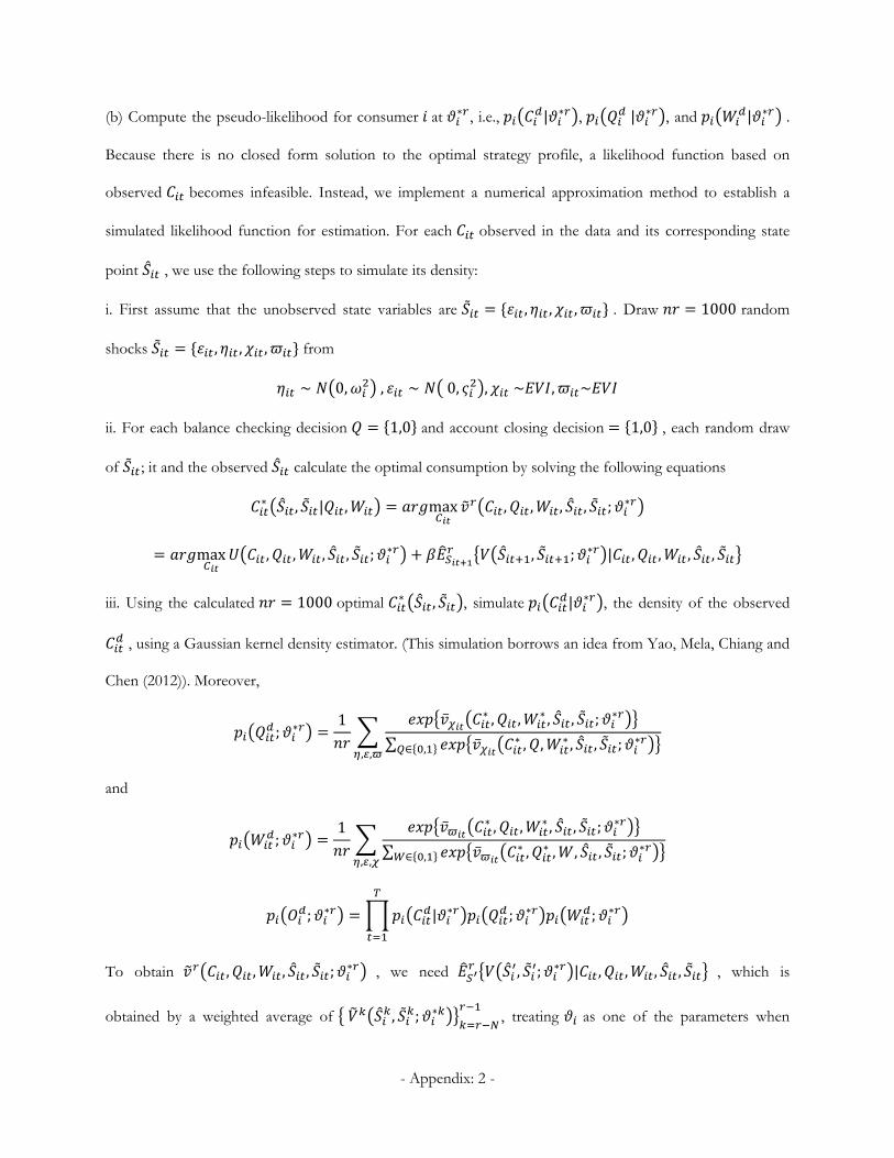
- Appendix: 2 -

(b) Compute the pseudo-likelihood for consumer at ∗ , i.e., | ∗ , | ∗ , and | ∗ .

Because there is no closed form solution to the optimal strategy profile, a likelihood function based on

observed becomes infeasible. Instead, we implement a numerical approximation method to establish a

simulated likelihood function for estimation. For each observed in the data and its corresponding state

point , we use the following steps to simulate its density:

i. First assume that the unobserved state variables are , , , . Draw 1000 random

shocks , , , from

∼ 0, , ∼ 0, , ~ , ~

ii. For each balance checking decision 1,0 and account closing decision 1,0 , each random draw

of ; it and the observed calculate the optimal consumption by solving the following equations

∗ , | , max , , , , ; ∗

max , , , , ; ∗ , ; ∗ | , , , ,

iii. Using the calculated 1000 optimal ∗ , , simulate | ∗ , the density of the observed

, using a Gaussian kernel density estimator. (This simulation borrows an idea from Yao, Mela, Chiang and

Chen (2012)). Moreover,

; ∗ 1 ̅ ∗ , , ∗ , , ; ∗

∑ ̅ ∗ , , ∗ , , ; ∗∈ ,, ,

and

; ∗ 1 ̅ ∗ , , ∗ , , ; ∗

∑ ̅ ∗ , ∗ , , , ; ∗∈ ,, ,

; ∗ | ∗ ; ∗ ; ∗

To obtain , , , , ; ∗ , we need , ; ∗ | , , , , , which is

obtained by a weighted average of , ; ∗ , treating as one of the parameters when

- Appendix: 3 -

computing the weights. In the case of independent kernels, for all , Ψ , , , , Γ , Ξ , ,

because , are continuous and evolve deterministically, Ψ and are continuous and evolve

stochastically, and , , , are discrete, so

, Ψ , , , , Γ , Ξ , , ; ∗ | , , , , Ψ , , , , Γ , Ξ , ,

, Ψ , , , , Γ , Ξ , , ; ∗∗ ∗ Ψ | , | , Ξ Ξ

∑ ∗ ∗ Ψ | , | , Ξ Ξ

We repeat the same step and obtain the pseudo-likelihood ; ∗ ) conditional on ( ).

We then determine whether or not to accept ∗ . The acceptance probability, , is given by

∗ ; , ; ∗ ∗ ,

; , ; , ∗

where ⋅ denotes the prior distribution.

(c) Repeat (a) & (b) for all i.

5. Computation of the pseudo-value function, , ; ∗

(a) Make one draw of the unobserved state variables from ∼ 0, , ∼ 0, ,

~ , ~ ;

(b) Compute the pseudo expected future value at ∗ .

, ; ∗ | , , , ,

, Ψ , , , , Γ , Ξ , , ; ∗∗ ∗ Ψ | , | , Ξ Ξ

∑ ∗ ∗ Ψ | , | , Ξ Ξ

(c) Compute , ; ∗ using the pseudo expected future values computed in (b) and the optimal

choices ∗, ∗, ∗.

, ; ∗ ∗, ∗, ∗, , ; ∗ , ; ∗ | ∗, ∗, ∗, ,

where ∗, ∗, ∗ satisfy

, ; ∗ max, ,

, , , , ; ∗ , ; ∗ | , , , ,

(d) Repeat (a-c) for all i.

6. Go to iteration 1.

- Appendix: 4 -

A3. Parallel MCMC Sampling Algorithm

Input: Subposterior samples, ~ , … , ~

Output: Posterior samples (asymptotically, as → ∞ ), ∼ . . . ∝ | 1: Set 1. 10: Draw ∼ 0,1 .

2: Draw ⋅ , . . . , 1, … ,∼ 11: if ⋅

⋅ then

3: Set ⋅ ⋅ . 12: Draw ∼ ̅ ⋅ , .

4: Draw ∼ ̅ ⋅, . 13: Set ⋅ ⋅ .

5: for 2 to do 14: else

6: for 1 to do 15: Draw ∼ ̅ ⋅ , .

7: Set ⋅ ⋅. 16: end if

8: Draw ∼ 1, … , 17: end for

9: Set . 18: end for

Table A2. Algorithm: Asymptotically Exact Sampling via a Nonparametric Density Product Estimation

A4. Model Comparison--Hit Rates for Non-incidents

A: No Forward

LookingB: No

InattentionC: No

Heterogeneity D: Proposed

Hit Rate: Overdraft 0.893 0.81 0.925 0.939Hit Rate: Check Balance 0.766 0.659 0.804 0.897Hit Rate: Close Account 0.885 0.853 0.901 0.916

Table A3. Model Comparison

A5. Predict Overdrafting

Instead of conditioning on overdrafting, we examine the factors that can predict whether a consumer

is going to overdraw and whether the consumer is a heavy overdrafter or a light overdrafter. The logistic

regressions in Table A4 show the following:

• Being younger or a student increases the likelihood that a consumer will overdraw and be a light overdrafter.

• Having low income increases the likelihood that a consumer will overdraw and be a heavy overdrafter.

• Having longer tenure/direct deposit/more debit/credit/mortgage accounts decreases the likelihood that a

consumer will overdraw or be a heavy overdrafter.

• Having more debit card transactions increases the likelihood that a consumer will overdraw and be a light

overdrafter.

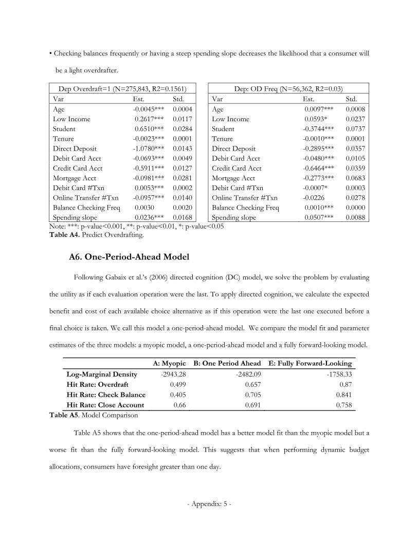
- Appendix: 5 -

• Checking balances frequently or having a steep spending slope decreases the likelihood that a consumer will

be a light overdrafter.

Dep Overdraft=1 (N=275,843, R2=0.1561) Dep: OD Freq (N=56,362, R2=0.03) Var Est. Std. Var Est. Std. Age -0.0045*** 0.0004 Age 0.0097*** 0.0008Low Income 0.2617*** 0.0117 Low Income 0.0593* 0.0237Student 0.6510*** 0.0284 Student -0.3744*** 0.0737Tenure -0.0023*** 0.0001 Tenure -0.0010*** 0.0001Direct Deposit -1.0780*** 0.0143 Direct Deposit -0.2895*** 0.0357Debit Card Acct -0.0693*** 0.0049 Debit Card Acct -0.0480*** 0.0105Credit Card Acct -0.5911*** 0.0127 Credit Card Acct -0.6464*** 0.0359Mortgage Acct -0.0981*** 0.0281 Mortgage Acct -0.2773*** 0.0683Debit Card #Txn 0.0053*** 0.0002 Debit Card #Txn -0.0007* 0.0003Online Transfer #Txn -0.0957*** 0.0140 Online Transfer #Txn -0.0226 0.0278Balance Checking Freq 0.0030 0.0020 Balance Checking Freq 0.0010*** 0.0000Spending slope 0.0236*** 0.0168 Spending slope 0.0507*** 0.0088

Note: ***: p-value<0.001, **: p-value<0.01, *: p-value<0.05 Table A4. Predict Overdrafting.

A6. One-Period-Ahead Model

Following Gabaix et al.’s (2006) directed cognition (DC) model, we solve the problem by evaluating

the utility as if each evaluation operation were the last. To apply directed cognition, we calculate the expected

benefit and cost of each available choice alternative as if this operation were the last one executed before a

final choice is taken. We call this model a one-period-ahead model. We compare the model fit and parameter

estimates of the three models: a myopic model, a one-period-ahead model and a fully forward-looking model.

A: Myopic B: One Period Ahead E: Fully Forward-Looking

Log-Marginal Density -2943.28 -2482.09 -1758.33Hit Rate: Overdraft 0.499 0.657 0.87Hit Rate: Check Balance 0.405 0.705 0.841Hit Rate: Close Account 0.66 0.691 0.758

Table A5. Model Comparison

Table A5 shows that the one-period-ahead model has a better model fit than the myopic model but a

worse fit than the fully forward-looking model. This suggests that when performing dynamic budget

allocations, consumers have foresight greater than one day.

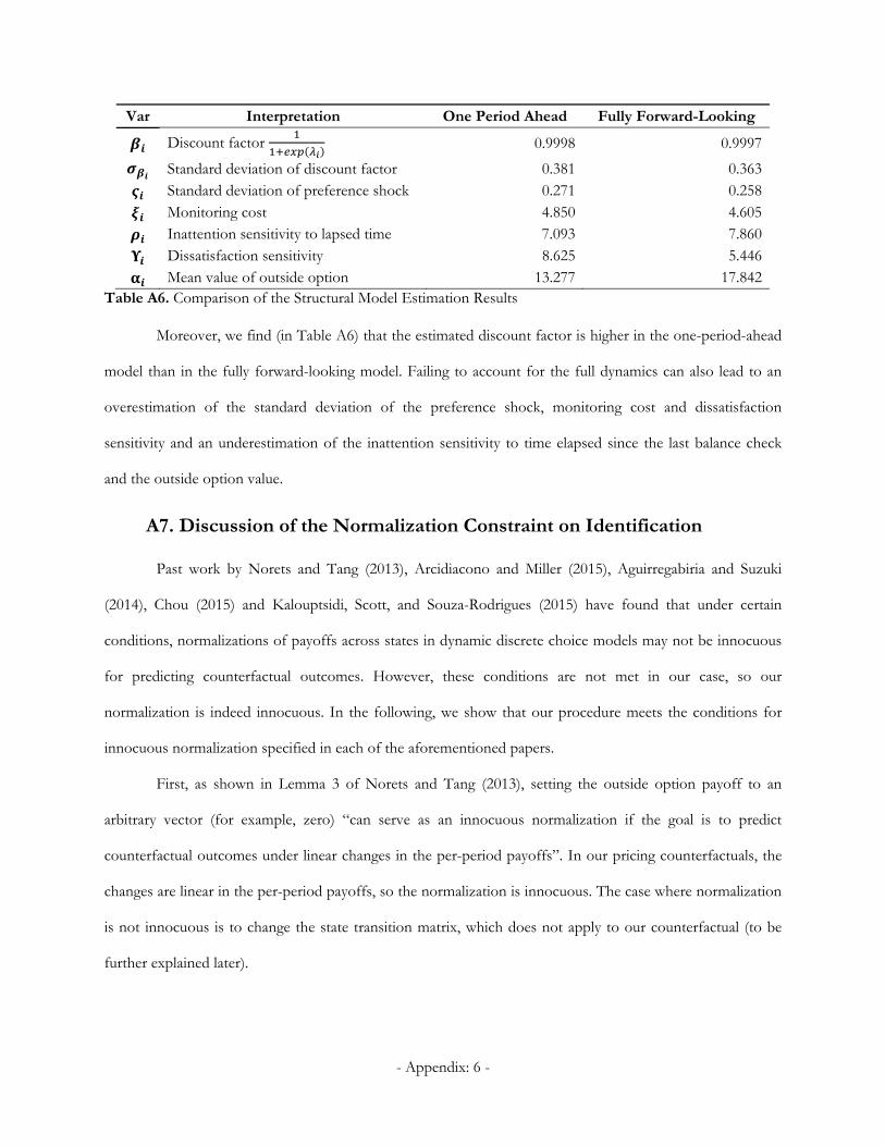
- Appendix: 6 -

Var Interpretation One Period Ahead Fully Forward-Looking

Discount factor 0.9998 0.9997

Standard deviation of discount factor 0.381 0.363

Standard deviation of preference shock 0.271 0.258

Monitoring cost 4.850 4.605

Inattention sensitivity to lapsed time 7.093 7.860

Dissatisfaction sensitivity 8.625 5.446

Mean value of outside option 13.277 17.842Table A6. Comparison of the Structural Model Estimation Results

Moreover, we find (in Table A6) that the estimated discount factor is higher in the one-period-ahead

model than in the fully forward-looking model. Failing to account for the full dynamics can also lead to an

overestimation of the standard deviation of the preference shock, monitoring cost and dissatisfaction

sensitivity and an underestimation of the inattention sensitivity to time elapsed since the last balance check

and the outside option value.

A7. Discussion of the Normalization Constraint on Identification

Past work by Norets and Tang (2013), Arcidiacono and Miller (2015), Aguirregabiria and Suzuki

(2014), Chou (2015) and Kalouptsidi, Scott, and Souza-Rodrigues (2015) have found that under certain

conditions, normalizations of payoffs across states in dynamic discrete choice models may not be innocuous

for predicting counterfactual outcomes. However, these conditions are not met in our case, so our

normalization is indeed innocuous. In the following, we show that our procedure meets the conditions for

innocuous normalization specified in each of the aforementioned papers.

First, as shown in Lemma 3 of Norets and Tang (2013), setting the outside option payoff to an

arbitrary vector (for example, zero) “can serve as an innocuous normalization if the goal is to predict

counterfactual outcomes under linear changes in the per-period payoffs”. In our pricing counterfactuals, the

changes are linear in the per-period payoffs, so the normalization is innocuous. The case where normalization

is not innocuous is to change the state transition matrix, which does not apply to our counterfactual (to be

further explained later).

- Appendix: 7 -

In addition, the examples in Appendix B of Chou (2015) change the state transition matrix, which

does not apply to our case. Moreover, Arcidiacono and Miller (2015) confirm that “counterfactual choice

probabilities for temporary policy changes are identified if the policy change only affects the flow payoffs,

though in the context of non-stationary finite horizon short panels”. In the setting of entry and exit game,

Aguirregabiria and Suzuki (2014) (Proposition 3 and Proposition 4) reinforce the findings that when

counterfactuals change only the per-period payoffs, rather than the discount factor or the state transition

matrix, identification is guaranteed. The same idea is supported by Kalouptsidi, Scott, and Souza-Rodrigues

(2015) (Proposition 21). In summary, as long as our counterfactual affects the per-period payoffs rather than

the state transition matrix, the normalization is innocuous.

Next, we show that our counterfactual affects only the per-period payoffs, not the state transition.

There are three dynamic choices in our model, one continuous, which is consumption, and two discrete,

which are balance check and account close. The normalization is applied to the discrete choice of account

close. Therefore, if the counterfactuals do not affect the state transitions related to this choice, then

normalization is innocuous. As shown in Blevin 2014, when both continuous and discrete choices are present,

the model can be decomposed into two stages. In stage one, the agent makes a discrete choice, then in stage

two, the agent makes a continuous choice given her previous discrete choice. As noted in Chow 2015, “the

advantage of using such a two-stage specification is that once the policy function of continuous choice is

identified, the optimal continuous choice can be viewed as an observable state variable”. Our model is a

direct application of this setup. After solving the optimal continuous choice problem for consumption, when

the agent is solving the optimal stopping problem of whether to close the account, the optimal consumption

can be treated as a state variable that affects only the per-period payoff. Thus, in the counterfactuals where we

change the pricing strategy from per-transaction fee to percentage fee or quantity-premium, the changes only

apply to the per-period payoff from consumption, not to the state transition related to the discrete choice of

account close. Let be the state variable that denotes the status of the account, whether open or not

( 1 is open and 0 is closed). In fact, the state transition

- Appendix: 8 -

| ,0, 01, 0 10, 1 1

is deterministic and does not change in the counterfactuals. Our conclusion is that the normalization used in

our model is innocuous for identification of the utility primitives and counterfactuals because of the nature of

the counterfactuals.

A8. Proof for Satisfying All the Assumptions of IJC’s

ASSUMPTION 1: Parameter space ⊆ is compact, that is, closed and bounded in the Euclidean space . The

proposal density , is continuously differentiable, strictly positive, and uniformly bounded in the parameter space given any

∈ .

In our model, the parameter space is compact in the Euclidean space. The proposal density is normal, so it is

continuously differentiable, strictly positive and uniformly bounded in the parameter space given any ∈ .

ASSUMPTION 2: For any ∈ , ∈ , and , ∈ , | , , , | for some 0 . Also,

, ,∙, is a nondecreasing function in and , ,∙,∙ satisfies the Lipschitz condition in terms of and θ. Also, the

density function , and the transition function | , , given a satisfy the Lipschitz condition.

In our model, , , , , , , , , . We assume 10 . Our per-

period utility function has additive error terms χ and ϖ, and another error term ε in the CRRA function.

0. Thus, is a nondecreasing function in all the

error terms.

, ,∙,∙ satisfies the Lipschitz condition because it is continuously differentiable in and θ in the compact

parameter space. The density functions for χ and ϖ are Type 1 extreme values, while the density function for

ε is normal. All of them satisfy the Lipschitz condition. Many state variables in the model are iid, including

bills ( ), income ( ), overdraft fee ( ), and all error terms ( , , ). The other state variables all

transit deterministically, including (perceived) balance ( ), days left until the next payday ( ), days since

- Appendix: 9 -

last balance check (Γ ), the ratio of the overdraft fee to the overdraft transaction amount (Ξ ) and open

status ( ). Deterministic transitions automatically satisfy the Lipschitz condition.

ASSUMPTION 3: is known, and 1.

Although we estimate in the model, the mean relative risk averse coefficient is assumed to be known.

Fixing one of the two is sufficient to identify the payoff function as well as counterfactual payoffs and the

convergence of IJC.

ASSUMPTION 4: For any ∈ , , and ∈ , , , for some 0. Furthermore, . ,

satisfies the Lipschitz condition in terms of and .

In iteration 0, we allow the expected value function to be 0. Thus, , , 1. As a result, the

Lipschitz condition is satisfied.

ASSUMPTION 5: is positive and bounded for any ∈ . Similarly, for any uniformly bounded ∈ and ,

, | , , 0 and is bounded and uniformly continuous in ∈ .

In our model, the prior for all is normal, and the prior for all hyper-parameters is diffuse normal. Thus, the

prior distribution is positive and bounded for any ∈ . Our likelihood function is bounded and uniformly

continuous in ∈ .

ASSUMPTION 6: is nondecreasing in , increases at most by one for a unit increase in , and →∞ .

Furthermore, → ∞ and there exists a finite constant 0 such that 1 for all 1, and,

for any 2, … , 1 1.

We set N=100. Because the number of iterations t=2000, all the requirements are satisfied.

ASSUMPTION 7: The bandwidth h is a nonincreasing function of and because →∞ , ℎ → 0 and

→ ∞. Furthermore, is constant for 1 .

We set h=0.01. All the conditions are satisfied.

ASSUMPTION 8: is a multivariate kernel with bandwidth 0. That is, 1/ / , where K

is a nonnegative, continuous, bounded real function that is symmetric around 0 and integrates to 1, that is, 1.

- Appendix: 10 -

Furthermore, ∞ and | | / for some positive constant , where for a vector ,

| | ,…, | |, and has an absolutely integrable Fourier transform.

We use the standard normal kernel, so it satisfies all the constraints.