Optimizing a Protocol for Fluorescence Recovery After...

Optimizing a Protocol for Fluorescence Recovery After

Photobleaching Experiments

Sarafa Adewale Iyaniwura ([email protected])African Institute for Mathematical Sciences (AIMS)

Supervised by: Professor Daniel Coombs

The University of British Columbia, Canada

22 May 2014

Submitted in partial fulfillment of a structured masters degree at AIMS South Africa

Abstract

Fluorescence Recovery After Photobleaching (FRAP) is a technique for estimating the mobility of flu-orescently tagged molecules in living cells. The most widely used tool for FRAP experiments is theConfocal Laser Scanning Microscope (CLSM) which allows the bleaching of arbitrary regions. DuringFRAP experiments with the CLSM, there is usually a trade-off between the time-step at which data areacquired and the size of the observation region. In this project, we developed several one-dimensionaland two-dimensional models for analysing FRAP data. We used these models to simulate FRAP recov-ery curves and then used the least square method to estimate the diffusion coefficient from the datagenerated. In addition to this, we provided the optimal locations in the bleached region and the optimaltiming for acquiring data during FRAP experiments in order to reduce the effect of the trade-off on theaccuracy of the data acquired.

Declaration

I, the undersigned, hereby declare that the work contained in this research project is my original work, andthat any work done by others or by myself previously has been acknowledged and referenced accordingly.

Sarafa Adewale Iyaniwura, 22 May 2014

i

Contents

Abstract i

1 Introduction 11.1 Fluorescence recovery after photobleaching . . . . . . . . . . . . . . . . . . . . . . . . . 11.2 Diffusion coefficient . . . . . . . . . . . . . . . . . . . . . . . . . . . . . . . . . . . . . 31.3 Mobile and Immobile fraction . . . . . . . . . . . . . . . . . . . . . . . . . . . . . . . . 31.4 Least square method . . . . . . . . . . . . . . . . . . . . . . . . . . . . . . . . . . . . 3

2 Model Derivation 42.1 Derivation of the one-dimensional models . . . . . . . . . . . . . . . . . . . . . . . . . 42.2 Derivation of the two-dimensional models . . . . . . . . . . . . . . . . . . . . . . . . . 9

3 FRAP analysis with different models 213.1 Description of the models . . . . . . . . . . . . . . . . . . . . . . . . . . . . . . . . . . 213.2 FRAP simulations . . . . . . . . . . . . . . . . . . . . . . . . . . . . . . . . . . . . . . 22

4 Optimizing FRAP experiment 274.1 Optimizing spatial location for data acquisition . . . . . . . . . . . . . . . . . . . . . . 274.2 Optimizing the timing for data acquisition . . . . . . . . . . . . . . . . . . . . . . . . . 29

5 Discussion and Conclusion 305.1 Discussion/Conclusion . . . . . . . . . . . . . . . . . . . . . . . . . . . . . . . . . . . . 305.2 Future work . . . . . . . . . . . . . . . . . . . . . . . . . . . . . . . . . . . . . . . . . 30

References 32

ii

1. Introduction

1.1 Fluorescence recovery after photobleaching

Fluorescence Recovery After Photobleaching (FRAP) is a technique for studying the mobility of moleculesin different media such as living cells. It was developed 40 years ago and was first used to study the lateraldiffusion of proteins and lipids in cell membranes. Lateral diffusion in cell membranes is well-establishedand varies according to the physiological state of living cells (Axelrod et al., 1976).

Photobleaching occurs when there is an irreversible breakdown of fluorescence in fluorophores as aresult of exposure to high intensity laser stimulation by wave lengths close to the excitation peak ofthe fluorophores. FRAP involves the bleaching of fluorescence in a small region of a surface containingfluorescent molecules, and then monitoring the random movement of molecules in and out of thebleached region. This movement increases the fluorescence intensity inside the bleached region until anequilibrium level of intensity is reached (Braga et al., 2004).

The classical method for FRAP experiments involved the use of non-scanning microscopes where bleach-ing is performed with a stationary laser beam that is focused on the samples. Nowadays, the most com-monly used tool for performing FRAP experiments is the Confocal Laser Scanning Microscope (CLSM)which is equipped with features such as acoustic-optic tunable filter (AOTF) that enables the bleachingof arbitrary regions in the sample. This feature makes the CLSM an excellent tool for performing FRAPexperiments. When using CLSM, the region to be bleached, the pattern and degree of bleaching arespecified in the software, after which the microscope scans the laser beam over the region in a sequen-tial pattern point-by-point and line-by-line, while modulating the intensity of the beam according to thespecified pattern (Braeckmans et al., 2003). The CLSM uses its laser to acquire images at low-intensityand for bleaching at high-intensity.

In a typical FRAP experiment to determine the mobility of specific proteins on a living cell surface,the protein of interest is fluorescently tagged. Images of the labelled protein are acquired at low-laserintensity in order to determine its pre-bleach fluorescent intensity. Next, high-laser intensity is used tobleach a small region of the cell surface for a short time. This region is referred to as the region ofinterest (ROI). After the bleaching, images of the fluorescence recovery process in the bleached regionare acquired at low-laser intensity and at specified time-steps. The total time of the experiment dependson the observed rate of recovery. The higher the mobility of the labelled protein, the shorter the recoverytime and thus, the shorter the time of the experiment.

The data obtained from FRAP experiments can be used to estimate the diffusion coefficient of thelabelled proteins, and the percentage of proteins that are immobile. The average diffusivity of theprotein is represented by the intensity of the recovered fluorescence. The form of recovery depends onfactors such as the mobility of the labelled protein, the size and shape of the region of interest, and theamount of bleaching.

Figure 1.1: FRAP experiment with 100% recovery.

1

Section 1.1. Fluorescence recovery after photobleaching Page 2

Figure 1.2: FRAP experiment with immobile fraction.

Figure 1.1 and 1.2 give a pictorial description of a typical FRAP experiment. Figure 1.1 involves asituation where all the proteins in the bleached region are able to move out of the region thereby leadingto 100% recovery while in Figure 1.2 we have a fraction of the protein that are unable to diffuse out ofthe bleached region leading to the remaining darker spot in the fourth image of the figure.

Figure 1.3: Recovery curve of FRAP experiment.

Figure 1.3 is the graphical representation of a typical data obtained from an ideal FRAP experiment.In this figure, Fi is the fluorescence intensity before photobleaching, F0 is the fluorescence intensityimmediately after photobleaching and F∞ is the fluorescence intensity after a long recovery time. Theslope of the curve is determined by the diffusivity of the labelled protein. The steeper the slope, thefaster the recovery and thus, the higher the diffusion coefficient.

There are technical problems encountered when using the CLSM for FRAP experiments. First, the lasertake a long time to bleach a rectangular strip. As a result of this, recovery may have started in someparts of the bleached region while bleaching is going on at other parts. There is a trade-off between thespeed of data acquisition and the size of the bleached region. In addition, the low-laser intensity usedfor data acquisition causes background bleaching which may affect the accuracy of the data acquired.

In this research project, we developed one-dimensional and two-dimensional models for analysing FRAPdata considering different bleach spots. We used these models to simulate FRAP data and then usedthe least square method to estimate the diffusion coefficient from the simulated data. We aimed atoptimizing the locations in the bleached region and the timing for data acquisition in FRAP experimentsin order to estimate the protein’s diffusion coefficient as accurately as possible.

Section 1.2. Diffusion coefficient Page 3

1.2 Diffusion coefficient

Diffusion from a molecular point of view, is based on the thermal motion of particles such as liquid andgas at temperatures above the absolute zero temperature, and describes the net flux of molecules froma region of high concentration to a region of low concentration. Diffusion is of great importance indisciplines such as chemistry, physics and biology. An important application of diffusion in cell biologyis in the transport of materials, e.g the transport of amino acids within cells.

The diffusion coefficient of a substance is the rate at which a mass of the substance diffuses througha unit time at a concentration gradient of unity . It indicates the diffusional mobility of a substanceand depends on some properties of the substance such as the sizes of its molecules among others. Thehigher the diffusion coefficient of a substance, the higher its diffusional mobility.

1.3 Mobile and Immobile fraction

In a FRAP experiment, it is expected that there will be fluorescence recovery in the bleached region.However, it is often difficult to have 100% fluorescence recovery after bleaching. This is as a result ofsome molecules in the bleached region that are unable to move out of the region. The fraction of thesemolecules is known as the immobile fraction. On the other hand, the fraction of the molecules that areable to diffuse out of the bleached region is known as the mobile fraction and it is defined as

Mf =F∞ − F0

Fi − F0(1.3.1)

where F∞, Fi, and F0 are as defined in Figure 1.1. Thus, the immobile fraction is 1−Mf .

1.4 Least square method

The Least square method is a popular technique in statistics for data fitting. It is widely used to estimatethe numerical values of the parameters used to fit a function to a set of data. The least square methodis categorised into two: the ordinary or linear least squares and the non-linear least squares. In thisproject, we used the ordinary least square method for estimating the diffusion coefficient from FRAPdata. This method involves minimizing the sum of squared difference over a set of possible values ofthe diffusion coefficient. It is given as

ssd(D) =N∑i=1

[di − (1− f)H(D, ti)]2 (1.4.1)

where D is a possible values of the diffusion coefficient, f is the immobile fraction, N is the number ofdata points, di are the FRAP data, and H(D, ti) are the intensity values from the model.

2. Model Derivation

In this chapter, we derive several Partial Differential Equations (PDEs) to model the fluorescence in-tensity in the bleached region of a cell during FRAP experiment. These PDEs vary in dimension anddepend on the geometry of the bleach region under consideration in the experiment. The equations weresolved using different methods and with FRAP like initial conditions. We then integrate the solutionsof these equations over the entire bleached region to get a function which can be used to predict thefluorescence intensity in the bleached region.

2.1 Derivation of the one-dimensional models

We begin by deriving the one-dimensional models which are used to model the bleaching of a rectangularstrip. These models are developed by using the one-dimensional diffusion equation,

1

D

∂f(x, t)

∂t=∂2f(x, t)

∂x2(2.1.1)

where f(x, t) is the fluorescence intensity at position x and time t, and D is the diffusion coefficient.

Figure 2.1: A rectangular strip bleach.

We developed these models using two different approaches which are the Fourier transforms and Fourierseries approach.

2.1.1 Fourier transform approach. This approach involves using the Fourier transforms in solvingEquation (2.1.1). In this approach, we assumed that the rectangular strip is infinite and that the bleachedregion has a width wb ([−a, a]). We also assumed that the initial fluorescent intensity everywhere onthe strip is unity except in the bleached region where the intensity is zero. This initial condition can bewritten as

f(x, 0) = φ(x) =

{0, −a ≤ x ≤ a1, otherwise.

(2.1.2)

First, let us define the Fourier transform of f(x, t) as

F [f(x, t)] = f̃(k, t) =

∫ ∞−∞

f(x, t)e−ikx dx , (2.1.3)

Then from Equation (2.1.1), we have∫ ∞−∞

∂f

∂te−ikx dx = D

∫ ∞−∞

∂2f

∂x2e−ikx dx

∂f̃

∂t= −Dk2f̃ . (2.1.4)

4

Section 2.1. Derivation of the one-dimensional models Page 5

Also, taking the Fourier transform of the initial condition, we obtain

f̃(k, 0) = φ̃(k) . (2.1.5)

We solved Equation (2.1.4), to get

f̃(k, t) = Ae−Dk2t (A is a constant) (2.1.6)

and then we apply the initial condition in Equation (2.1.5) to the solution in Equation (2.1.6),

f̃(k, t) = φ̃(k)e−Dk2t . (2.1.7)

From the products and convolution properties of Fourier transforms,

F [h ∗ g] = F [h] ·F [g] = h̃ · g̃ (2.1.8)

where

(h ∗ g)(x) =

∫ ∞−∞

h(ζ)g(x− ζ) dζ . (2.1.9)

Also, we know that

F

e−x2a2a√π

= e−k2a2

4 .

If we let a2/4 = Dt, then a =√

4Dt and so,

F

e−x2

4Dt

√4Dtπ

= e−Dk2t . (2.1.10)

Now, applying Equations (2.1.8), (2.1.9) and (2.1.10) to Equation (2.1.7), we have

f(x, t) =

∫ ∞−∞

φ(ζ)

e− (x−ζ)24Dt

√4Dtπ

dζ ,

f(x, t) =1√

4Dtπ

∫ ∞−∞

φ(ζ)e−(x−ζ)2

4Dt dζ , (2.1.11)

Applying the initial condition in Equation (2.1.2) to Equation (2.1.11), we obtained

f(x, t) =

∫ −a−∞

e−(x−ζ)24Dt

√4Dtπ

dζ +

∫ ∞a

e−(x−ζ)24Dt

√4Dtπ

dζ . (2.1.12)

If we let (ζ−x)√4Dt

= s, then dζ =√

4Dt ds. Substituting for s in Equation (2.1.12), we have

f(x, t) =1√π

∫ −(a+x)√4Dt

−∞e−s

2ds+

1√π

∫ ∞(a−x)√

4Dt

e−s2

ds ,


and since

1√π

∫ ∞−∞

e−s2

ds = 1 ,

it follows that

f(x, t) =

(1− 1√

π

∫ ∞−(a+x)√

4Dt

e−s2

ds

)+

1√π

∫ ∞(a−x)√

4Dt

e−s2

ds

= 1− 1

2erfc

(−(a+ x)√

4Dt

)+

1

2erfc

(a− x√

4Dt

)

= 1− 1

2

(1 + erf

(a+ x√

4Dt

))+

1

2

(1− erf

(a− x√

4Dt

)).

Simplifying, we obtain

f(x, t) = 1− 1

2erf

(a+ x√

4Dt

)− 1

2erf

(a− x√

4Dt

)(2.1.13)

where erf is the usual error function.

This is the solution of the diffusion equation in Equation (2.1.1) with respect to our initial condition.

Next, we integrate the function f(x, t) as defined in Equation (2.1.13) over the entire bleached regionto get

H(t,D) =2√Dt√π

[1− exp

(−a2

Dt

)]+ 2a

[erf

(a√Dt

)− 1

].

Since wb = 2a, we have

H(t,D) =2√Dt√π

[1− exp

(−w2

b

4Dt

)]+ wb

[erf

(wb

2√Dt

)− 1

](2.1.14)

where wb is the width of the bleach region and D is the diffusion coefficient of the proteins.

This is the model for the Fourier transforms approach.

2.1.2 Fourier Series approach. In this approach, we used separation of variables and Fourier seriesmethod to solve the diffusion equation in Equation (2.1.1). Here, we assumed that the rectangular stripis of finite length Lc = 2L ([−L,L]) and the bleached region is of width wb = 2a ([−a, a] ⊂ [−L,L]).In developing this model, we also assumed that the boundaries of the strip satisfy the Neumann boundaryconditions below.

fx(−L, t) = fx(L, t) = 0 . (2.1.15)

We begin by using the method of separation of variable. Let

f(x, t) = X(x)T (t) .


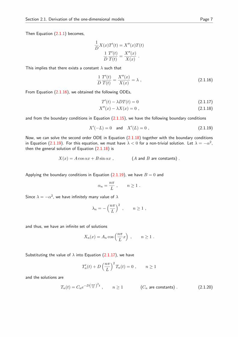
Then Equation (2.1.1) becomes,

1

DX(x)T ′(t) = X ′′(x)T (t)

1

D

T ′(t)

T (t)=X ′′(x)

X(x).

This implies that there exists a constant λ such that

1

D

T ′(t)

T (t)=X ′′(x)

X(x)= λ , (2.1.16)

From Equation (2.1.16), we obtained the following ODEs,

T ′(t)− λDT (t) = 0 (2.1.17)

X ′′(x)− λX(x) = 0 , (2.1.18)

and from the boundary conditions in Equation (2.1.15), we have the following boundary conditions

X ′(−L) = 0 and X ′(L) = 0 , (2.1.19)

Now, we can solve the second order ODE in Equation (2.1.18) together with the boundary conditionsin Equation (2.1.19). For this equation, we must have λ < 0 for a non-trivial solution. Let λ = −α2,then the general solution of Equation (2.1.18) is

X(x) = A cosαx+B sinαx , (A and B are constants) .

Applying the boundary conditions in Equation (2.1.19), we have B = 0 and

αn =nπ

L, n ≥ 1 .

Since λ = −α2, we have infinitely many value of λ

λn = −(nπL

)2, n ≥ 1 ,

and thus, we have an infinite set of solutions

Xn(x) = An cos(nπLx), n ≥ 1 .

Substituting the value of λ into Equation (2.1.17), we have

T ′n(t) +D(nπL

)2Tn(t) = 0 , n ≥ 1

and the solutions are

Tn(t) = Cne−D(nπL )

2t , n ≥ 1 (Cn are constants) . (2.1.20)


Recall, f(x, t) = X(x)T (t), therefore, fn(x, t) = Xn(x)Tn(t). Thus,

fn(x, t) = AnCn cos(nπLx)e−D(nπL )

2t

fn(x, t) = an cos(nπLx)e−D(nπL )

2t , (AnCn = an) .

Using the principle of superposition, we have

f(x, t) =a02

+∑n≥1

an cos(nπLx)e−D(nπL )

2t . (2.1.21)

Here, our initial condition is

f(x, 0) = φ(x) =

{0, −a ≤ x ≤ a1, otherwise.

(2.1.22)

Applying this initial condition, we have

a02

+∑n≥1

an cos(nπLx)

= φ(x) . (2.1.23)

To get a0, we integrate each term of this equation over the interval [−L,L],∫ L

−L

a02

dx+∑n≥1

an

∫ L

−Lcos(nπLx)

dx =

∫ L

−Lφ(x) dx ,

from this equation, we have

a0 =1

L

∫ L

−Lφ(x) dx .

Implementing the step function in the initial condition in Equation (2.1.22) gives

a0 = 2(

1− a

L

). (2.1.24)

Similarly, to get an, we multiply each term of Equation (2.1.23) by cos(nπL x)

and then integrate over[−L,L]

a02

∫ L

−Lcos(nπLx)

dx+∑n≥1

an

∫ L

−Lcos(nπLx)

cos(nπLx)

dx =

∫ L

−Lφ(x) cos

(nπLx)

dx .

Since ∫ L

−Lcos2

(nπLx)

dx = L and

∫ L

−Lcos(nπLx)

dx = 0,

we have

an =1

L

∫ L

−Lφ(x) cos

(nπLx)

dx .

Section 2.2. Derivation of the two-dimensional models Page 9

Also, implementing the step function in the initial condition in Equation (2.1.22) gives

an = − 2

nπsin(nπaL

x). (2.1.25)

Therefore,

f(x, t) =(

1− a

L

)−∑n≥1

(2

nπsin(nπaL

))cos(nπLx)e−D(nπL )

2t . (2.1.26)

Next, we integrate the function f(x, t) as defined in Equation (2.1.26) over the entire bleached region,

H(t,D) =

∫ a

−a

(1− a

L

)dx−

∫ a

−a

∑n≥1

(2

nπsin(nπaL

))e−D(nπL )

2t cos

(nπLx)

dx ,

evaluating the integral and simplifying, we have

H(t,D) = 2a(

1− a

L

)−∑n≥1

4L

n2π2sin2

(nπaL

)e−D(nπL )

2t .

Since the length of the cell Lc = 2L and the width of the bleached region wb = 2a , then we can writethis equations as

H(t,D) = wb

(1− wb

Lc

)− 2Lc

π2

∑n≥1

1

n2sin2

(nπ wbLc

)e−D

(2nπLc

)2t. (2.1.27)

This is the model for the Fourier Series approach.

2.2 Derivation of the two-dimensional models

For the two-dimensional models, we considered the disc bleach spot (Figure 2.2) and the square bleachspot (Figure 2.3). These models can be used to model the mobility of protein in a cell membrane.

2.2.1 Disk bleach spot. In developing a model for this bleach spot, we consider the diffusion equationin the cylindrical coordinate given as

1

r

∂V

∂r+∂2V

∂r2+

1

r2∂2V

∂θ2=

1

D

∂V

∂t, (2.2.1)

where V (r, θ, t) is the fluorescence intensity on the disc at time t and 0 ≤ r ≤ a is the radius of thedisc.

With the boundary conditions,

|V (0, θ, t)| <∞ , V (r, 0, t) = V (r, 2π, t) , and Vθ(r, 0, t) = Vθ(r, 2π, t) , 0 ≤ r ≤ a (2.2.2)

V (a, θ, t) = 1 , 0 ≤ θ ≤ 2π and t ≥ 0 . (2.2.3)


Figure 2.2: A disc bleach spot.

We assumed that the initial fluorescent intensity everywhere on the cell surface is unity except in theinterior part of the disc where it is zero as a result of bleaching, i.e

V (r, θ, 0) = φ(r, θ) = 0 , 0 ≤ r < a (2.2.4)

and that the intensity at the edge of the disc is unity at all time (this is satisfied by the boundarycondition in Equation (2.2.3)).

We begin by partitioning the desired solution into two solutions as shown below,

V (r, θ, t) = w(r, θ) + u(r, θ, t) (2.2.5)

where w(r, θ) is the steady-state solution and u(r, θ, t) is the time-dependent solution.

In our case, we make the steady-state solution to be a constant (w(r, θ) = 1), therefore,

V (r, θ, t) = 1 + u(r, θ, t) . (2.2.6)

Substituting V (r, θ, t) as defined in Equation (2.2.6) into Equation (2.2.1), we have

1

r

∂u

∂r+∂2u

∂r2+

1

r2∂2u

∂θ2=

1

D

∂u

∂t. (2.2.7)

This equation satisfies the boundary conditions,

|u(0, θ, t)| <∞ , u(r, 0, t) = u(r, 2π, t) , and uθ(r, 0, t) = uθ(r, 2π, t) , 0 ≤ r ≤ a , (2.2.8)

u(a, θ, t) = 0 , 0 ≤ θ ≤ 2π , t ≥ 0 . (2.2.9)

Now, we can solve Equation (2.2.7) together with the boundary conditions in Equations (2.2.8) and(2.2.9). Using the method of separation of variables, let

u(r, θ, t) = R(r)Θ(θ)T (t) ,

then Equation (2.2.7) becomes,

1

rR′(r)Θ(θ)T (t) +R′′(r)Θ(θ)T (t) +

1

r2R(r)Θ′′(θ)T (t) =

1

DR(r)Θ(θ)T ′(t) .


We divide each term of this equation by R(r)Θ(θ)T (t), to obtain

1

r

R′(r)

R(r)+R′′(r)

R(r)+

1

r2Θ′′(θ)

Θ(θ)=

1

D

T ′(t)

T (t),

and this implies that there exists a constant −α2 such that

1

r

R′(r)

R(r)+R′′(r)

R(r)+

1

r2Θ′′(θ)

Θ(θ)=

1

D

T ′(t)

T (t)= −α2 .

From this equation, we have

1

D

T ′(t)

T (t)= −α2

T ′(t)+α2DT (t) = 0

and

1

r

R′(r)

R(r)+R′′(r)

R(r)+

1

r2Θ′′(θ)

Θ(θ)= −α2

1rR′(r)Θ(θ) +R′′(r)Θ(θ) + 1

r2R(r)Θ′′(θ)

R(r)Θ(θ)= −α2 .

Multiply both sides of this equation by r2 to get

rR′(r) + r2R′′(r) + r2α2R(r)

R(r)= −Θ′′(θ)

Θ(θ).

This also implies that there exists another constant β2 such that

rR′(r) + r2R′′(r) + r2α2R(r)

R(r)= −Θ′′(θ)

Θ(θ)= β2 , (2.2.10)

Form Equation (2.2.10), we have

rR′(r) + r2R′′(r) + r2α2R(r)

R(r)= β2 .

Simplifying this equation, we obtain

r2R′′(r) + rR′(r) + (r2α2 − β2)R(r) = 0 .

Also, form Equation (2.2.10), we have

−Θ′′(θ)

Θ(θ)= β2

Θ′′(θ) + β2Θ(θ) = 0


Therefore, the PDE in Equation (2.2.7) has been transform into the following ODEs

T ′(t)+α2DT (t) = 0 , (2.2.11)

r2R′′(r) + rR′(r)+(r2α2 − β2)R(r) = 0 , (2.2.12)

Θ′′(θ)+β2Θ(θ) = 0 . (2.2.13)

From the boundary conditions in Equation (2.2.8), we have

u(r, 0, t) = u(r, 2π, t) =⇒ R(r) Θ(0)T (t) = R(r) Θ(2π)T (t) =⇒ Θ(0) = Θ(2π)

uθ(r, 0, t) = uθ(r, 2π, t) =⇒ R(r) Θ′(0)T (t) = R(r) Θ′(2π)T (t) =⇒ Θ′(0) = Θ′(2π) .

Solving the second order ODE in Equation (2.2.13), we obtain the general solution

Θ(θ) = A cos θβ +B sin θβ , (A and B are constants) .

Applying the boundary conditions

Θ(0) = Θ(2π) and Θ′(0) = Θ′(2π) ,

we have

A = A cos 2πβ and B = B cos 2πβ .

For these equations to hold, β must be an integer, therefore, β = n , n = 0, 1, 2, . . . . Thus, thesolution of the boundary value problem is

Θn(θ) = An cosnθ +Bn sinnθ , n = 0, 1, 2, . . .

Now, let us consider Equation (2.2.12)

r2R′′(r) + rR′(r)+(r2α2 − β2)R(r) = 0 .

Since β = n, we have

r2R′′n(r) + rR′n(r)+(r2α2 − n2)Rn(r) = 0 , n = 0, 1, 2, . . . (2.2.14)

We can use the method of Frobenius to obtain the general solution

Rn(r) = Cn Jn(αr) + En Yn(αr) (2.2.15)

where Cn and En are constants,

Jn(αr) =

∞∑k=0

(−1)k

k! Γ(k + n+ 1)

(αr2

)2k+nand J−n(αr) =

∞∑k=0

(−1)k

k! Γ(k − n+ 1)

(αr2

)2k−n

are Bessel functions of the first kind of order n and order −n respectively.

Yn(αr) =cos(nπ)Jn(αr)− J−n(αr)

sin(nπ), αr > 0


is a Bessel function of the second kind of order n.

From the boundary conditions |u(0, θ, t)| <∞ and u(a, θ, t) = 0, we derived |R(0)| <∞ and R(a) = 0.We need to apply these boundary conditions to the solution in Equation (2.2.15).

For |R(0)| < ∞, we know that |Jn(αr)| ≤ 1 for n = 0, 1, 2, . . . . But as r −→ 0, Yn(αr) −→ −∞.Therefore, for the condition |R(0)| < ∞ to hold, En must be zero and so, Rn(r) = Cn Jn(αr). ForR(a) = 0,

Rn(a) = CnJn(αa) = 0

Cn 6= 0, ∴ Jn(αa) = 0 .

Since the Bessel function behaves in a sinusoidal way, Jn(αa) = 0 for infinitely many α for each n.That is

Jn(αnia) = 0 for i = 1, 2, . . .

where αni is the ith zero of the Bessel function of order n.

Rni(r) = Cni Jn(αnir) n = 0, 1, 2, . . . , i = 1, 2, . . .

From Equation (2.2.11), we have

T ′ni(t) + αniDTni(t) = 0 .

Solving this equation, we obtain

Tni(t) = Gnie−α2

niDt (Gni, constant).

Recall, u(r, θ, t) = R(r)Θ(θ)T (T ), therefore, uni(r, θ, t) = Rni(r)Θn(θ)Tni(T ). Thus,

uni(r, θ, t) = CniJn(αnir)(An cosnθ +Bn sinnθ)Gnie−α2

niDt. (2.2.16)

Using the principle of superposition, we have

u(r, θ, t) =∞∑n=0

∞∑i=0

CniJn(αnir)(An cosnθ +Bn sinnθ)Gnie−α2

niDt

u(r, θ, t) =

∞∑n=0

∞∑i=0

Jn(αnir)(ani cosnθ + bni sinnθ)e−α2niDt (ani = CniAn, bni = CniBn) .

We recall from Equation (2.2.6) that

V (r, θ, t) = 1 + u(r, θ, t) .

Therefore,

V (r, θ, t) = 1 +∞∑n=0

∞∑i=0

Jn(αnir)(ani cosnθ + bni sinnθ)e−α2niDt. (2.2.17)


We assumed that the distribution of fluorescence intensity on the disc is symmetric and does not dependon the angle θ, therefore, the solution of Equation (2.2.1) becomes:

V (r, t) = 1 +

∞∑i=0

di J0(αir)e−α2

iDt (di, constant) (2.2.18)

and the initial condition in Equation (2.2.4) becomes

V (r, 0) = φ(r) = 0 , 0 ≤ r < a (2.2.19)

Now, let us apply the initial condition in Equation (2.2.19) to the solution in Equation (2.2.18). Applyingthis conditions, we have

1 +

∞∑i=0

di J0(αir) = 0 .

If we then multiply both sides of this result by rJ0(αir) and integrate from 0 to a,∫ a

0r J0(αir)di J0(αir) dr = −

∫ a

0r J0(αir)dr

di =−∫ a0 r J0(αir)dr∫ a

0 r [J0(αir)]2 dr

=−2

a αi J1(αi a).

Therefore,

V (r, t) = 1−∞∑i=0

(2

a αi J1(αi a)

)J0(αir) e

−α2iDt .

Next, we integrate the function V (r, t) over the entire bleached region (the disc),

H(t,D) =

∫ a

02πr dr−

∫ a

0

∞∑i=0

2πr

(2

a αi J1(αi a)

)J0(αir) e

−α2iDt dr

= 2π

∫ a

0r dr−

∞∑i=0

(4π

a αi J1(αi a)

)e−α

2iDt

∫ a

0rJ0(αir) dr

= 2π

[r2

2

]a0

−∞∑i=0

4πe−α2iDt

a αi J1(αi a)

(aJ1(αi a)

αi

).

Simplifying this equation, we get

H(t,D) = a2π −∞∑i=0

4π

α2i

e−α2iDt

where a is the radius of the disc and αi is the ith zero of the Bessel function of the first kind of orderzero.

This function can be used to model the FRAP experiment with a disc bleach spot.


Figure 2.3: A square bleach spot.

2.2.2 Square bleach spot. In deriving the model for the square bleach spot, we used the two-dimensionaldiffusion equation in xy coordinates given by

1

D

∂u

∂t=∂2u

∂x2+∂2u

∂y2(2.2.20)

where u(x, y, t) is the fluorescence intensity at position (x, y) and time t, and D is the diffusion coeffi-cient.

We assumed the surface of the cell is a square with sides Lc = 2L ([−L,L]× [−L,L]) and the bleachedregion is a smaller square on the surface of the cell with sides Lb = 2a ([−a, a] × [−a, a]). We alsoassumed the boundaries of the cell satisfies the Neumann boundary conditions,

ux(−L, y, t) = ux(L, y, t) = 0 (2.2.21)

uy(x,−L, t) = uy(x, L, t) = 0 ,

and that the initial fluorescence intensity on the cell surface is unity everywhere except in the bleachedregion where the intensity is zero. This can be written as

u(x, y, 0) = φ(x, y) =

{0, −a ≤ x ≤ a , −a ≤ y ≤ a1, otherwise.

(2.2.22)

We begin by using the method of separation of variables. Let

u(x, y, t) = X(x)Y (y)T (t) ,

then Equation (2.2.20) becomes

1

DX(x)Y (y)T ′(t) = X ′′(x)Y (y)T (t) +X(x)Y ′′(y)T (t) .

Dividing each term of this equation by X(x)Y (y)T (t), we obtain

1

D

T ′(t)

T (t)=X ′′(x)

X(x)+Y ′′(y)

Y (y).


Let

1

D

T ′(t)

T (t)=X ′′(x)

X(x)+Y ′′(y)

Y (y)= −(α2 + β2) . (2.2.23)

From this equation, we have

1

D

T ′(t)

T (t)= −(α2 + β2) ,

T ′(t) + (α2 + β2)DT (t) = 0 .

Also, from Equation (2.2.23),

X ′′(x)

X(x)+Y ′′(y)

Y (y)= −(α2 + β2)

X ′′(x)

X(x)+ α2 = −

(Y ′′(y)

Y (y)+ β2

).

For this equation to hold, both sides of the equation must be equal to zero. That is,

X ′′(x)

X(x)+ α2 = 0 and

Y ′′(y)

Y (y)+ β2 = 0

X ′′(x) + α2X(x) = 0 Y ′′(y) + β2Y (y) = 0 .

We have transformed the PDE in Equation (2.2.20) into the following ODEs

T ′(t) + (α2 + β2)DT (t) = 0 (2.2.24)

X ′′(x) + α2X(x) = 0 (2.2.25)

Y ′′(y) + β2Y (y) = 0 . (2.2.26)

From the boundary conditions in Equation (2.2.21), we have

X ′(−L) = X ′(L) = 0 (2.2.27)

Y ′(−L) = Y ′(L) = 0 . (2.2.28)

Now, let us consider the ODE in Equation (2.2.25). The general solution of this equation is

X(x) = A cosαx+B sinαx , (A and B are constants)

Applying the boundary conditions in Equation (2.2.27) to this solution, we have

B = 0 and αn =nπ

L, n ≥ 1

∴ Xn(x) = An cos(nπLx), n ≥ 1 . (2.2.29)

Similarly, the general solution of Equation (2.2.26) is

Y (y) = C cosβy +G sinβy , (C and G are constants)

and applying the boundary conditions in Equation (2.2.28), we have

G = 0 and βm =mπ

L, m ≥ 1

∴ Ym(x) = Cm cos(mπLy), m ≥ 1 . (2.2.30)


Substituting αn = nπL and βm = mπ

L into Equation (2.2.24), we obtain

T ′n,m(t) +D

((nπL

)2+(mπL

)2)Tn,m(t) = 0 , n,m ≥ 1

and the solution of this equation is

Tn,m(t) = En,me−D π2

L2 (n2+m2)t , n,m ≥ 1. (2.2.31)

Recall that u(x, y, t) = X(x)Y (y)T (t), therefore, un,m(x, y, t) = Xn(x)Ym(y)Tn,m(t). Substitutingthe results in Equations (2.2.29), (2.2.30) and (2.2.31) into this equation,

un,m(x, y, t) = An cos(nπLx)Cm cos

(mπLy)En,me

−D π2

L2 (n2+m2)t .

Using the principle of superposition,

u(x, y, t) = u0,0(x, y, t) +∑n≥1

un,0(x, y, t) +∑m≥1

u0,m(x, y, t) +∑n≥1

∑m≥1

un,m(x, y, t)

u(x, y, t) = a0,0 +∑n≥1

an,0 cos(nπLx)e−D

π2

L2 n2t +

∑m≥1

a0,m cos(mπLy)e−D

π2

L2m2t

+∑n≥1

∑m≥1

An cos(nπLx)Cm cos

(mπLy)En,me

−D π2

L2 (n2+m2)t .

Therefore, the general solution of the PDE in Equation (2.2.20) is

u(x, y, t) = a0,0 +∑n≥1

an,0 cos(nπLx)e−D

π2

L2 n2t +

∑m≥1

a0,m cos(mπLy)e−D

π2

L2m2t

+∑n≥1

∑m≥1

an,m cos(nπLx)

cos(mπLy)e−D

π2

L2 (n2+m2)t , (AnCmEn,m = an,m)

(2.2.32)

Next, we apply the initial condition in Equation (2.2.22). This initial condition can be written in theform

u(x, y, 0) = φ(x, y) =

1, −L ≤ x < −a , −L ≤ y ≤ L1, −a ≤ x ≤ a , −L ≤ y < −a0, −a ≤ x ≤ a , −a ≤ y ≤ a1, a < x ≤ L , −L ≤ y ≤ L1, −a ≤ x ≤ a , a < y ≤ L

(2.2.33)

First, we apply the initial condition as function of φ(x, y),

u(x, y, 0) = a0,0 +∑n≥1

an,0 cos(nπLx)

+∑m≥1

a0,m cos(mπLy)

+∑n≥1

∑m≥1

an,m cos(nπLx)

cos(mπLy)

= φ(x, y) . (2.2.34)


To get a00, we integrate each term of the equation over the square ([−L,L]× [−L,L])∫ L

−L

∫ L

−La0,0 dx dy +

∑n≥1

an,0

∫ L

−L

∫ L

−Lcos(nπLx)

dx dy

+∑m≥1

a0,m

∫ L

−L

∫ L

−Lcos(mπLy)

dx dy

+∑n≥1

∑m≥1

an,m

∫ L

−L

∫ L

−Lcos(nπLx)

cos(mπLy)

dx dy =

∫ L

−L

∫ L

−Lφ(x, y) dx dy . (2.2.35)

Since ∫ L

−Lcos(nπLx)

dx = 0 and

∫ L

−Lcos(nπLy)

dy = 0 , (2.2.36)

Equation (2.2.35), reduces to∫ L

−L

∫ L

−La0,0 dx dy =

∫ L

−L

∫ L

−Lφ(x, y) dx dy

a0,0 =1

4L2

∫ L

−L

∫ L

−Lφ(x, y) dx dy .

Implementing the step function in the initial condition in Equation (2.2.33), we have

a0,0 =1

4L2

[∫ −a−L

∫ L

−L1 dx dy +

∫ a

−a

∫ −a−L

1 dx dy +

∫ a

−a

∫ a

−a0 dx dy

+

∫ L

a

∫ L

−Ldx dy +

∫ a

−a

∫ L

a1 dx dy

]a0,0 = 1− a2

L2.

To get an,0, we multiply each term of Equation (2.2.34) by cos(nπL x)

and then integrate over the square([−L,L]× [−L,L]),∫ L

−L

∫ L

−La0,0 cos

(nπLx)

dx dy +∑n≥1

an,0

∫ L

−L

∫ L

−Lcos2

(nπLx)

dx dy

+∑m≥1

a0,m

∫ L

−L

∫ L

−Lcos(nπLx)

cos(mπLy)

dx dy

+∑n≥1

∑m≥1

an,m

∫ L

−L

∫ L

−Lcos2

(nπLx)

cos(mπLy)

dx dy

=

∫ L

−L

∫ L

−Lφ(x, y) cos

(nπLx)

dx dy . (2.2.37)

Based on the results in Equation (2.2.36), Equation (2.2.37) reduces to

an,0

∫ L

−L

∫ L

−Lcos2

(nπLx)

dx dy =

∫ L

−L

∫ L

−Lφ(x, y) cos

(nπLx)

dx dy

an,0 =1

2L2

∫ L

−L

∫ L

−Lφ(x, y) cos

(nπLx)

dx dy .



an,0 =1

2L2

[∫ −a−L

∫ L

−Lcos(nπLx)

dx dy +

∫ a

−a

∫ −a−L

cos(nπLx)

dx dy

+

∫ a

−a

∫ a

−a0 dx dy +

∫ L

a

∫ L

−Lcos(nπLx)

dx dy +

∫ a

−a

∫ L

acos(nπLx)

dx dy

]an,0 = − 2a

nπLsin(nπLa).

Similarly, to get a0,m, we multiply each term of Equation (2.2.34) by cos(mπL y)

and then integrate overthe square ([−L,L]× [−L,L]),∫ L

−L

∫ L

−La0,0 cos

(mπLy)

dx dy +∑n≥1

an,0

∫ L

−L

∫ L

−Lcos(mπLy)

cos(nπLx)

dx dy

+∑m≥1

a0,m

∫ L

−L

∫ L

−Lcos2

(mπLy)

dx dy +∑n≥1

∑m≥1

an,m

∫ L

−L

∫ L

−Lcos(nπLx)

cos2(mπLy)

dx dy

=

∫ L

−L

∫ L

−Lφ(x, y) cos

(mπLy)

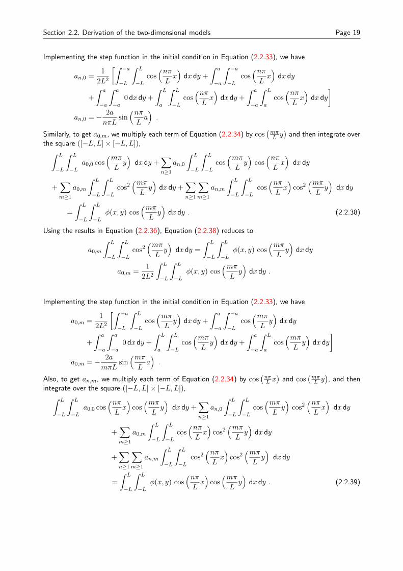
dx dy . (2.2.38)

Using the results in Equation (2.2.36), Equation (2.2.38) reduces to

a0,m

∫ L

−L

∫ L

−Lcos2

(mπLy)

dx dy =

∫ L

−L

∫ L

−Lφ(x, y) cos

(mπLy)

dx dy

a0,m =1

2L2

∫ L

−L

∫ L

−Lφ(x, y) cos

(mπLy)

dx dy .


a0,m =1

2L2

[∫ −a−L

∫ L

−Lcos(mπLy)

dx dy +

∫ a

−a

∫ −a−L

cos(mπLy)

dx dy

+

∫ a

−a

∫ a

−a0 dx dy +

∫ L

a

∫ L

−Lcos(mπLy)

dx dy +

∫ a

−a

∫ L

acos(mπLy)

dx dy

]a0,m = − 2a

mπLsin(mπLa).

Also, to get an,m, we multiply each term of Equation (2.2.34) by cos(nπL x)

and cos(mπL y), and then

integrate over the square ([−L,L]× [−L,L]),∫ L

−L

∫ L

−La0,0 cos

(nπLx)

cos(mπLy)

dx dy +∑n≥1

an,0

∫ L

−L

∫ L

−Lcos(mπLy)

cos2(nπLx)

dx dy

+∑m≥1

a0,m

∫ L

−L

∫ L

−Lcos(nπLx)

cos2(mπLy)

dx dy

+∑n≥1

∑m≥1

an,m

∫ L

−L

∫ L

−Lcos2

(nπLx)

cos2(mπLy)

dx dy

=

∫ L

−L

∫ L

−Lφ(x, y) cos

(nπLx)

cos(mπLy)

dx dy . (2.2.39)


Using the results in Equation (2.2.36),

an,m =1

L2

∫ L

−L

∫ L

−Lφ(x, y) cos

(nπLx)

cos(mπLy)

dx dy .

Implementing the step function in the initial condition in Equation (2.2.33),

an,m = − 4

nmπ2sin(nπLa)

sin(mπLa).

Substituting the values of a0,0, an,0, a0,m, and an,m into Equation (2.2.32), we have

u(x, y, t) =

(1− a2

L2

)− 2a

L

∑n≥1

1

nπsin(nπLa)

cos(nπLx)e−D

π2

L2 n2t

− 2a

L

∑m≥1

1

mπsin(mπLa)

cos(mπLy)e−D

π2

L2m2t

− 4∑n≥1

∑m≥1

1

nmπ2sin(nπLa)

sin(mπLa)

cos(nπLx)

cos(mπLy)e−D

π2

L2 (n2+m2)t .

(2.2.40)

We integrate the function u(x, y, t) as defined in Equation (2.2.40) over the bleach region (([−a, a]×[−a, a]))

H(t,D) =

∫ a

−a

∫ a

−a

(1− a2

L2

)dx dy − 2a

L

∑n≥1

1

nπsin(nπLa)e−D

π2

L2 n2t∫ a

−a

∫ a

−acos(nπLx)

dx dy

− 2a

L

∑m≥1

1

mπsin(mπLa)e−D

π2

L2m2t∫ a

−a

∫ a

−acos(mπLy)

dx dy

− 4∑n≥1

∑m≥1

1

nmπ2sin(nπLa)

sin(mπLa)e−D

π2

L2 (n2+m2)t∫ a

−a

∫ a

−acos(nπLx)

cos(mπLy)

dx dy

H(t,D) = 4a2(

1− a2

L2

)− 8a2

π2

∑n≥1

1

n2sin2

(nπLa)e−D

π2

L2 n2t − 8a2

π2

∑m≥1

1

m2sin2

(mπLa)e−D

π2

L2m2t

− 16L2

π4

∑n≥1

∑m≥1

1

n2m2sin2

(nπLa)

sin2(mπLa)e−D

π2

L2 (n2+m2)t .

Since Lc = 2L and Lb = 2a, we have

H(t,D) = L2b

(1−

L2b

L2c

)−

2L2b

π2

∑n≥1

1

n2sin2

(nπLbLc

)e−4D π2

L2cn2t

−2L2

b

π2

∑m≥1

1

m2sin2

(mπLbLc

)e−4D π2

L2cm2t

− 4L2c

π4

∑n≥1

∑m≥1

1

n2m2sin2

(nπLbLc

)sin2

(mπLbLc

)e−4D π2

L2c(n2+m2)t

(2.2.41)

where Lc is the length of each side of the cell surface, Lb is the length of each side of the bleach regionand D is the diffusion coefficient of the proteins.

This is the model for the square bleach spot.

3. FRAP analysis with different models

In this chapter, we analyse FRAP experiments using the models we developed. We used these models tosimulate a typical FRAP recovery curve and then used the least square method to estimate the simulateddiffusion coefficient from the data generated. We also analysed the effect of noise and immobile fractionon our ability to fit the diffusion coefficient accurately.

3.1 Description of the models

3.1.1 One dimensional models. We begin by describing the one-dimensional models which are rea-sonable approximations of bleaching a rectangular strip. These models were developed by using theone-dimensional diffusion equation given in Equation (2.1.1). In developing the one-dimensional mod-els, this equation was solved using two different approaches which are the Fourier transforms and Fourierseries approach. The Fourier transforms method assumes the cell surface is infinite while the FourierSeries method assumes it is finite.

For the Fourier transform method, we considered a bleach region of width wb and as initial condition,we assumed that the initial fluorescence intensity is unity everywhere on the strip except in the bleachedregion where it is zero as a result of the bleaching. In order to obtain our model, we integrated thesolution of the diffusion equation over the entire bleached region. The model for this method is givenas

H(t,D) =2√Dt√π

[1− exp

(−w2

b

4Dt

)]+ wb

[erf

(wb

2√Dt

)− 1

](3.1.1)

where erf is the usual error function, D is the diffusion coefficient of the proteins and wb is the widthof the bleached region.

(See chapter two for detailed derivation of the model.)

In deriving the Fourier series model, we assumed that the cell has a length Lc and a bleach regionof width wb. We used the same initial condition as that of the Fourier transforms approach and thensolved the diffusion equation in Equation (2.1.1) using the method of separation of variables and Fourierseries method. The solution obtained was integrated over the bleached region to obtain our model. TheFourier series model is,

H(t,D) = wb

(1− wb

Lc

)− 2Lc

π2

∑n≥1

1

n2sin2

(nπ wbLc

)e−D

(2nπLc

)2t

(3.1.2)

where Lc is the length of the cell, wb is the width of the bleached region and D is the diffusion coefficientof the proteins.


3.1.2 Two dimensional models. For this case, we considered the square bleach spot and the discbleach spot. For a disc bleach spot, we used the diffusion equation in cylindrical coordinates to developthe model but assumed that there is no diffusion in the z-coordinate (Equation (2.2.1)). We assumedthat the radius of the disc is a and that the cell surface is infinite. We also assumed the fluorescenceintensity on the boundary of the disc is unity at all time and that the initial intensity in the interior

21

Section 3.2. FRAP simulations Page 22

part of the disc is zero, simulating the bleached region. We solved the diffusion equation in Equation(2.2.1) with these initial and boundary conditions and assumed that there is symmetry in the diffusion offluorescence on the disc. The solution of the diffusion equation was integrated over the entire bleachedregion in order to obtain our model. The model is given as

H(t,D) = a2π −∞∑i=0

4π

α2i

e−α2iDt (3.1.3)

where a is the radius of the disc and αi is the ith zero of the Bessel function of the first kind of orderzero.


In modelling a FRAP experiment with a square bleach spot, we used the two-dimensional diffusionequation in xy coordinates given in Equation (2.2.20). We assumed the surface of the cell is a squareof sides Lc and that the bleached region is a smaller square of sides Lb on the surface of the cell (SeeFigure 2.3).

In addition to this, we assumed that the fluorescence intensity everywhere on the cell surface is unityexcept in the bleached region (smaller square) where the intensity is zero. We solved the diffusionequation in Equation (2.2.20) using separation of variables and Fourier series method and then integratethe solution over the entire bleach region. Our model in this case is given as

H(t,D) = L2b

(1−

L2b

L2c

)−

2L2b

π2

∑n≥1

1

n2sin2

(nπLbLc

)e−4D π2

L2cn2t

−2L2

b

π2

∑m≥1

1

m2sin2

(mπLbLc

)e−4D π2

L2cm2t

− 4L2c

π4

∑n≥1

∑m≥1

1

n2m2sin2

(nπLbLc

)sin2

(mπLbLc

)e−4D π2

L2c(n2+m2)t

(3.1.4)

where Lc is the length of each side of the cell, Lb is the length of each side of the bleach region and Dis the diffusion coefficient of the proteins.


3.2 FRAP simulations

In this sections, we used the models developed to simulate FRAP recovery curves and then used the leastsquare method to fit the diffusion coefficient from the generated data. All simulation were carried outusing Sage. We evaluated our models at different time points with a known value of diffusion coefficientover a specified time interval. The value of these models at each time point gives the fluorescenceintensity in the bleached region at the specified time. The data generated were used to simulate FRAPcurves. Figures 3.1 shows the data generated using the one-dimensional Fourier transforms and Fourierseries models. We considered a bleached region of 2µm for these models and for the Fourier seriesmodel, we assumed a cell of length 10µm.


Figure 3.1: Simulated FRAP recovery curves us-ing the 1D models.

Figure 3.2: Fitting the diffusion coefficient usingsimulated data in Figure 3.1

In generating these FRAP curves, we considered 70 time points at 1 Hz, a diffusion coefficient ofD = 0.05 µm/s and mobile fraction Mf = 1 (which means that we have 100% recovery). The 1Dmodels predict the same fluorescence intensity in the bleached regions except at the few time points.After simulating the curves, we used the least square method to estimate the diffusion coefficient fromthe data. We were able to estimate D accurately from the generated data ( See Figures 3.2).

For the disc bleach spot, we used the model in Equation (3.1.3) and considered a disc of radius 1, 70time points, D = 0.05µm2/s and Mf = 1 (Figure 3.3). We were also able to recover the diffusioncoefficient from the generated data accurately (Figure 3.4). The simulated FRAP curve for the squarebleach spot is displayed in Figure 3.5. This curve was generated using the model in Equation (3.1.4),and considering a cell surface area of 100µm2. It is recommended that the bleached region should belocated at the center of the cell and that it should be less than 5% of the total surface area of the cellin order to estimate the diffusion coefficient as accurate as possible (Dushek and Coombs, 2008). Inaccordance with this, we chose a bleach region of 4µm2 located at the center of the cell (See Figure2.3 for example). In this case, we also considered 70 data points, D = 0.05µm2/s and Mf = 1. Thenwe used the least square method to fit the diffusion coefficient from the simulated data ( Figure 3.6).

Figure 3.3: Simulated FRAP recovery curvegenerated using the model in Equation (3.1.3).

Figure 3.4: Fitting the diffusion coefficient usingsimulated data in Figure 3.3.


Figure 3.5: Simulated FRAP recovery curvegenerated using the model in Equation (3.1.4).

Figure 3.6: Fitting the diffusion coefficient usingsimulated data in Figure 3.5.

Next, we investigate the effect of noise on our ability to estimate the diffusion coefficient. To do this,we generated FRAP data with 15% gaussian noise and tried to fit the diffusion coefficient from thenoisy data. Figure 3.7 shows an example of a noisy data from FRAP experiment. For this case, the 1Dmodels estimated the diffusion coefficient as 0.05µm/s (Figure 3.8) while the 2D models estimated itas 0.06µm2/s with an error of 20% (Figure 3.9 and Figure 3.10) .

Figure 3.7: Simulated data with 15% gaussiannoise.

Figure 3.8: Fitting the diffusion coefficient fromdata with 15% noise using the 1D models.


Figure 3.9: Fitting the diffusion coefficient fromdata simulated with 15% noise using the modelin Equation (3.1.4).

Figure 3.10: Fitting the diffusion coefficientfrom data simulated with 15% noise using themodel in Equation (3.1.3).

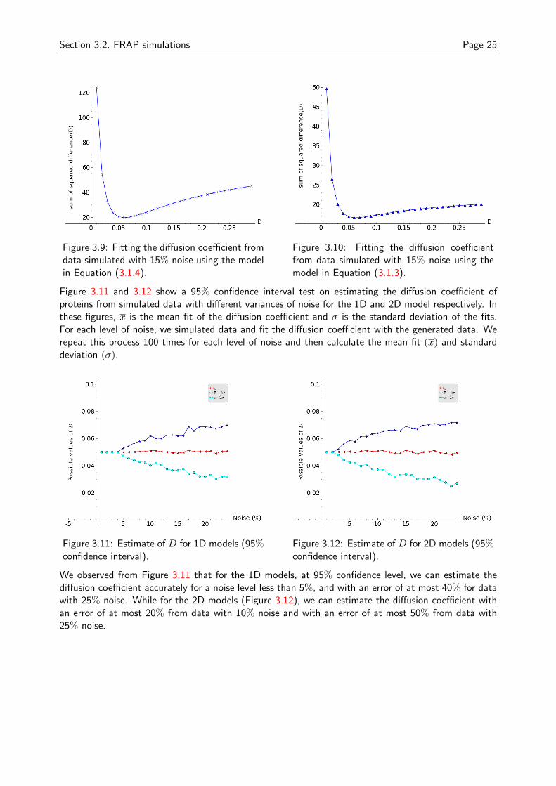
Figure 3.11 and 3.12 show a 95% confidence interval test on estimating the diffusion coefficient ofproteins from simulated data with different variances of noise for the 1D and 2D model respectively. Inthese figures, x is the mean fit of the diffusion coefficient and σ is the standard deviation of the fits.For each level of noise, we simulated data and fit the diffusion coefficient with the generated data. Werepeat this process 100 times for each level of noise and then calculate the mean fit (x) and standarddeviation (σ).

Figure 3.11: Estimate of D for 1D models (95%confidence interval).

Figure 3.12: Estimate of D for 2D models (95%confidence interval).

We observed from Figure 3.11 that for the 1D models, at 95% confidence level, we can estimate thediffusion coefficient accurately for a noise level less than 5%, and with an error of at most 40% for datawith 25% noise. While for the 2D models (Figure 3.12), we can estimate the diffusion coefficient withan error of at most 20% from data with 10% noise and with an error of at most 50% from data with25% noise.


Since it is often difficult to have 100% fluorescence recovery during FRAP experiment, in addition tothe effect of noise, we also investigated the effect of immobile fraction on our ability to fit the diffusioncoefficient. We used data simulated with 15% gaussian noise and assumed that 5% of the proteins areimmobile. In recovering the diffusion coefficient, the 1D models estimated D as 0.06µm/s, the squarebleach model estimated it as 0.06µm2/s while the other 2D model estimated it as 0.07µm2/s with60% accuracy. These results are displayed in Figures 3.13 and 3.14 for the 1D models, Figure 3.16 forthe square bleach model and Figure 3.15 for the disc bleach model.

Figure 3.13: Fitting the diffusion coefficientfrom data simulated with 15% noise and 5%immobile fraction using the model in Equation(3.1.1).




4. Optimizing FRAP experiment

In this chapter, we optimize our ability to estimate the diffusion coefficient as accurate as possible eitherby acquiring data at specified locations in the bleached region during recovery or by acquiring the imageof the entire bleached region at specified time points. This will help reduce the effect of the trade-offbetween the speed of data acquisition and the size of the bleached region, and also reduce the effectof background bleaching that occurs during data acquisition. All the investigations in the chapter arebased on simulations and all simulations were carried out using Sage.

4.1 Optimizing spatial location for data acquisition

In this section, we optimize our ability to acquire data at a faster rate during FRAP experiment. Since theuse the CLSM for FRAP experiment requires sequential scanning of the cell surface for data acquisition,we intend to acquire data only at specified locations of the bleached region in order the reduce the timetaken to scan the entire bleached region and also to reduce the number of images acquired. This willhelp reduce the error in the data acquired as a result of the trade-off and background bleaching.

We considered the case of bleaching a rectangular strip, and simulated FRAP data using the 1D model inEquation (3.1.1). We partitioned the bleached region into equal sub-intervals and sampled fluorescenceintensity in the region at period intervals instead of considering the entire region. These sampledintensities were used to estimate the average fluorescence intensity in the bleached region and also tofit the diffusion coefficient. We intend to find the optimal region for data sampling and also the optimalnumber of sub-intervals to be considered in order to estimate the diffusion coefficient as accurate aspossible.

Figure 4.1: Partitioning the bleached region

Figure 4.1 shows the partitioning of a bleached region into equal sub-intervals. In this figure, everysecond sub-interval is selected and the selected sub-intervals are shaded in blue.

Since diffusion in this case is one-dimensional, we expect to have symmetry of fluorescence intensityabout the middle of the bleached region with the highest intensity at the edges of the region. Therefore,

27

Section 4.1. Optimizing spatial location for data acquisition Page 28

including the sub-intervals containing the two edges of the bleached region among the sampled sub-intervals will lead to over estimating the fluorescence intensity in the region. We carried out severalexperiments on this, considering different sizes of bleached region and different sub-intervals in theregions. Our experiment also shows that including the sub-intervals that contains the two edges of thebleached region among the sampled sub-intervals (Figure 4.1b) leads to over estimating the averagefluorescence intensity in the region (except all the sub-intervals are considered), thereby giving a lessaccurate estimate of the diffusion coefficient. Including only one of the edges (See Figure 4.1a) gives abetter estimate than including both.

In order to get the best estimate of the diffusion coefficient, the sampled intervals must exclude bothedges of the bleached region. To achieve this, we partitioned the bleached region into sub-intervals andthen select the sub-intervals in a periodic manner, such that non of the sub-intervals containing theedges are included in the selection (Figure 4.1c).

First, we considered selecting every second sub-interval, and then used the integrated fluorescenceintensity in the intervals to predict the average fluorescence intensity in the bleached region. Thisaverage intensity is used to estimate the diffusion coefficient.

Next, we selected every third sub-intervals and then every fourth. Following the same procedure, theresults obtained are similar. But the best estimate was obtained when every second sub-interval isselected as shown in Figure 4.1.

Figure 4.2: Fitting the diffusion coefficient by considering fluorescence intensity in different sub-intervalsof the bleached region.

We initially carried out the investigation with data simulated without noise. Since a typical FRAP datacontains noise, we simulated data with different variances of guassian noise and performed the sameinvestigation. The results obtained in all cases are similar. Figure 4.2 shows the results of a particularcase where different sub-intervals of the bleached region were considered. In this case, we considereda bleached region of width 4µm, D=0.05µm/s, Mf = 1 and simulated data with 15% gaussian noise.In fitting the diffusion coefficient, we partitioned the bleached region into sub-intervals and considereddifferent selections of the sub-intervals. When the sub-intervals containing the two edges of the bleachedregion were included in the sampling, the diffusion coefficient was estimated as 0.01µm with 80% error,and including only one of the edges, we obtained 0.02µm, that is with 60% error. In the case whereneither of the two edges was considered, the diffusion coefficient was estimated as 0.04µm, with 20%error. We observed that the best estimate was obtained when neither of the two edges was included.

Section 4.2. Optimizing the timing for data acquisition Page 29

4.2 Optimizing the timing for data acquisition

In this section, we optimize the timing for data acquisition during FRAP experiment by acquiring fewerimages during fluorescence recovery thereby reducing the amount of background bleaching that occursduring data acquisition.

For this investigation, we also considered bleaching a rectangular strip and assumed that we can acquirean image of the entire bleached region at once. We used the 1D models and considered different sizesof bleached region. The result are similar for both models and for all sizes of bleached region.

First, we simulated data without noise and considered fitting the diffusion coefficient from the datausing only one time point and assuming Mf = 1. We were able to estimate the diffusion coefficientaccurately irrespective of the time point considered. In addition to this, we considered using more thanone time point and we were still able to estimate D accurately. In this case, the number of data pointsconsidered and the timing of the data does not affect the accuracy of the estimate. Next, we assumedthere is an immobile fraction. In this situation, we were unable to estimate the diffusion coefficientaccurately.

Furthermore, we simulated data with 15% gaussian noise and tried to fit the diffusion coefficient withfew time points. We observed that considering only one time point, the point close to the beginning offluorescence recovery give better estimate than others. And considering more than one time point, thepoints should be considerably spaced with more point at the beginning of the recovery. Also, at leasttwo time points are required for estimates with high degree of accuracy (Figure 4.4). We varied thelevel of noise, and the results are similar for all noise variances.

Figure 4.3: Fitting the diffusion coefficient usingfew time points (without noise).

Figure 4.4: Fitting the diffusion coefficient usingdifferent numbers of time points.

Figure 4.3 shows a case where only two time points were considered for estimating D with Mf = 1 andthe same time points were also used with Mf = 0.9. Figure 4.4 shows a case where different numbersof time points where considered. The data used in this case was simulated with 20% gaussian noise andMf = 1. When we used only one time point, D was estimated as 0.19µm/s, when we considered twotime points, it was estimated as 0.03µm/s and with three time points, it was estimated as 0.04µm/s.

5. Discussion and Conclusion

5.1 Discussion/Conclusion

We have developed several models for FRAP experiments with respect to different geometries of bleachedregion. We have 1D models for bleaching a rectangular strip, a model for a square bleach spot andanother for a disc bleach spot. We used these models to simulate FRAP recovery curve and then usedthe least square method to fit the diffusion coefficient from the simulated data.

We have also analysed the effect of noise and immobile fraction on our ability to fit the diffusioncoefficient accurately. We observed that with a noise level of 15%, we were able to estimate thediffusion coefficient accurately for the 1D models and with at least 80% accuracy for the 2D models.Also, with a 15% noise level and an immobile fraction of 5%, we were able to recover D with 80%accuracy for the 1D model and with at least 60% accuracy for the 2D models. This shows that noiseand immobile fraction affects the accuracy of our fitting.

In addition, we investigated the robustness of the least square method as a technique for fitting diffusioncoefficient from FRAP data. We carried out a 95% confidence interval test on this method using differentvariances of noise. For the 1D models, we estimated the diffusion coefficient accurately from simulateddata with less than 5% noise and with an error of at most 40% from data with 25% noise. And forthe 2D models, at 95% confidence level, we estimated the diffusion coefficient with an error of at most20% from simulated data with 10% noise and at most 50% error for data with 25% noise.

Also, we provided a systematic way of sampling fluorescence intensity in the bleached region for 1Dbleaching in order to reduce the effect of the trade-off between the speed of data acquisition and thesize of the bleached region on the accuracy of the data acquired. This systematic sampling involvessampling fluorescence intensity in some selected sub-regions of the bleached region and then estimatingthe average intensity in the bleached region based on the sampled intensity. This technique will helpreduce the time taken by the scanner to scan the entire bleached region. Using this approach, weobserved that sampling fluorescence intensity at the two edges of the bleached region leads to overestimating the average intensity in the region and therefore, gives a less accurate estimate of D. Andto get the best estimate of the diffusion coefficient, we must exclude sampling the fluorescence intensityat the two edges of the bleached region.

Furthermore, we provided a technique of reducing the noise in the data acquired during FRAP ex-periments as a result of background bleaching that occurs during image acquisition. This techniqueinvolves taking fewer images. We discovered that we can also estimate the diffusion coefficient with ahigh degree of accuracy by taking fewer images during fluorescence recovery. These images should notbe acquired at consecutive time intervals, there should be a considerable time spacing between themwith more images at the beginning of the recovery. Choosing the time of image acquisition carefullycould be of benefit to the experimentalist.

5.2 Future work

Future work in this area may include further optimization of the locations and timing of data acquisitionfor 2D bleaching. In addition, the finite speed of the camera used in acquiring images may be explicitlyincluded in the analysis.

30

Acknowledgements

My greatest thanks to Almighty God for the gift of life.

I would like to express my deep gratitude to my supervisor Professor Daniel Coombs for his valuableand constructive suggestions during the planning and development of this research work. And also, tomy tutor Markus Kruger for his patience, guidance, enthusiatic encouragement and useful critiques ofthis research.

In addition, I would like to thank Dr. Sehun Chun for his assistance during this research and the entireAIMS family for their support during my studies at AIMS South Africa.

Finally, I wish to dedicate this project to my late parents and my siblings.

31

References

R. B. Adeniyi. Basic essential topics in mathematical methods. Evidence Nigeria Ventures, 2007.

D. Axelrod, D. E. Koppel, J. Schlessinger, E. Elson, and W. W. Webb. Mobility measurement by analysisof fluorescence photobleaching recovery kinetics. Biophysical Journal, 16:1055 – 1069, 1976.

K. Braeckmans, L. Peeters, N. N. Sanders, S. C. D. Smedt, and J. Demeester. Three-Dimensionalfluorescence recovery after photobleaching with the confocal scanning laser microscope. BiophysicalJournal, 85(4):2240–2252, 2003.

J. Braga, J. M. Desterro, and M. Carmo-Fonseca. Intracellular macromolecular mobility measuredby fluorescence recovery after photobleaching with confocal laser scanning microscopes. Journal ofBiochemical and Biophysical Methods, 15(10):4749–4760, 2004.

O. Dushek and D. Coombs. Improving parameter estimation for cell surface FRAP data. Journal ofBiochemical and Biophysical Methods, 70(6):1224–1231, 2008. ISSN 0165-022X. doi: 10.1016/j.jbbm.2007.07.002. URL http://www.sciencedirect.com/science/article/pii/S0165022X07001443.

G. C. Everstine. Analytic Solution of Partial Differential Equations. 2012.

J. S. Goodwin and A. K. Kenworthy. Photobleaching approaches to investigate diffusional mobility andtrafficking of ras in living cells. Methods, 37(2):154–164, 2005. ISSN 1046-2023. doi: 10.1016/j.ymeth.2005.05.013. URL http://www.sciencedirect.com/science/article/pii/S1046202305001301.

Mostinsky, I.L. Diffusion coefficient. Thermopedia, http://www.thermopedia.com/content/696/, Ac-cessed April 2014.

Sage. Sage Mathematics Software (Version 6.1). The Sage Development Team, 2014. URL http://www.sagemath.org.

Y. Sniekers and C. van Donkelaar. Determining diffusion coefficients in inhomogeneous tissues usingfluorescence recovery after photobleaching. Biophysical Journal, 89(2):1302–1307, 2005. ISSN 0006-3495. doi: 10.1529/biophysj.104.053652. URL http://www.sciencedirect.com/science/article/pii/S0006349505727776.

Wikipedia (2014). Mass diffusivity. Wikipedia, the Free Encyclopedia, a. URL http://en.wikipedia.org/wiki/Mass diffusivity.

Wikipedia (2014). Least squares. Wikipedia, the Free Encyclopedia, b. URL http://en.wikipedia.org/wiki/Leastsquare.

32

http://www.sciencedirect.com/science/article/pii/S0165022X07001443

http://www.sciencedirect.com/science/article/pii/S1046202305001301

http://www.thermopedia.com/content/696/

http://www.sagemath.org

http://www.sagemath.org



http://en.wikipedia.org/wiki/Mass_diffusivity

http://en.wikipedia.org/wiki/Mass_diffusivity

http://en.wikipedia.org/wiki/Least square

http://en.wikipedia.org/wiki/Least square

Optimizing a Protocol for Fluorescence Recovery After...

Documents

Transcript of Optimizing a Protocol for Fluorescence Recovery After...