Optimizing a Parallel1D CSEM Application

Srinivasa Ravindra Ongole

7/16/2009

MSc in High Performance Computing

The University of Edinburgh

Year of Presentation: 2009

Table of Contents Chapter 1- Introduction ....................................................................................................... 7

1.2 Objective of the Project ............................................................................................. 8

Chapter 2- Background Information and Literature review................................................ 9

2.1 CSEM Technique ......................................................................................................... 9

2.1.1 Origin of CSEM .................................................................................................... 9

2.1.2 Implementation of CSEM .................................................................................... 9

2.2 Existing Framework .................................................................................................. 11

2.2.1 Read Input data ................................................................................................. 12

2.2.2 Frequency Domain Computation ...................................................................... 12

2.2.3 Time Domain Computation ............................................................................... 16

2.2.3 Adaptive stopping ............................................................................................. 18

2.2.4 Write solution to file ......................................................................................... 18

2.3 Software development life cycle .............................................................................. 19

2.4 Tools and External Libraries Utilized ........................................................................ 20

2.4.1 netCDF4 (network Common Data Forum) [11]................................................. 20

2.4.2 HDF5 (Hierarchical Data Format 5) [14] ........................................................... 20

2.4.3 Vampirtrace ....................................................................................................... 21

2.4.4 Allinea Opt [17] ................................................................................................. 21

2.4.5 Pearson’s Correlation Coefficient ..................................................................... 21

2.4.6 Platforms ........................................................................................................... 22

Chapter 3- Benchmarking the existing framework ........................................................... 23

3.1 Hotspot Analysis ....................................................................................................... 23

3.2 Scalability of the application .................................................................................... 24

3.3 Effect of problem size on performance ................................................................... 26

3.4 Load Balance ............................................................................................................ 27

3.5 Communication overheads ...................................................................................... 27

3.5.1 Allinea opt test .................................................................................................. 28

3.5.2 Vampirtrace analysis ......................................................................................... 29

3.6 Correctness of Adaptive stopping technique........................................................... 32

3.6.1 Test 1: Without adaptive stopping ................................................................... 33

3.6.2 Test 2: With adaptive stopping ......................................................................... 34

3.6.3 Analysis of Test 1 and Test 2 results ................................................................. 36

3.7 File IO ........................................................................................................................ 37

3.8 Conclusions............................................................................................................... 38

Chapter 4 ........................................................................................................................... 39

4.1 Frequency domain computation .............................................................................. 39

4.1.1 Objective ........................................................................................................... 39

4.1.2 Design ................................................................................................................ 39

4.1.3 Performance analysis ........................................................................................ 42

4.2 Time Domain Integration ......................................................................................... 48

4.2.1 Design .................................................................................................................... 48

4.2.2 Load balance ..................................................................................................... 53

4.3 File IO .................................................................................................................... 53

4.4 Performance comparison of new framework with existing framework ................. 55

Chapter 5 ........................................................................................................................... 62

Conclusions and Future work ......................................................................................... 62

5.1 Conclusions............................................................................................................... 62

5.2 Future work .............................................................................................................. 62

Adaptive Stopping technique ..................................................................................... 62

Parallel netCDF4 ......................................................................................................... 63

Porting the code to higher kernels ............................................................................ 63

Bibliography ....................................................................................................................... 64

Table of Figures Figure 1: A simple CSEM model ......................................................................................... 10

Figure 2 : CSEm Process flow ............................................................................................. 11

Figure 3 Frequency Domain Solution ................................................................................ 13

Figure 4 Frequency domain computation process flow .................................................... 15

Figure 5 Time domain integration ..................................................................................... 16

Figure 6 time domain solution computed for 10000 frequency points. ........................... 17

Figure 7 Software life cycle ................................................................................................ 19

Figure 8: HDF5 Implementation ........................................................................................ 21

Figure 9 Hotsopot Analysis ................................................................................................ 23

Figure 10: Runtime vs Number of processors ................................................................... 24

Figure 11: Parallel efficiency .............................................................................................. 25

Figure 12 Paralle efficienciy of the application for different problem sizes ..................... 26

Figure 13 Communication Overhead analysis ECDF ......................................................... 28

Figure 14 COMMUNICATION OVERHEAD ANALYSIS NESS ................................................ 29

Figure 15 Vampirtrace Global timeline ............................................................................. 30

Figure 16 Overall time taken ............................................................................................. 31

Figure 17Computation and Communication time line with Allinea Opt on ECDF ............ 32

Figure 18: Time domain solutions for different frequenct step sizes ............................... 34

Figure 19 Time Domain solutions obtained for different adaptive stopping criterion .... 35

Figure 20 Runtime vs Number of processors .................................................................... 42

Figure 21Paralel efficiency of New framework ................................................................. 43

Figure 22 comparison Runtimes for different problem sizes ............................................ 44

Figure 23 Overlapping Parabolas ....................................................................................... 49

Figure 24 Error of Integration in different integration schemes ...................................... 52

Figure 25Frequency domain solution New framework .................................................... 56

Figure 26 Frequency domain solution Existing framework ............................................... 57

Figure 27 Comparision of Runtimes .................................................................................. 58

Figure 28Allinea Opt test ................................................................................................... 59

Table Index Table 1: Load Balance ........................................................................................................ 27

Table 2 Comparison of accuracy using Pearson's Correlation coefficient ........................ 33

Table 3 Comparison of accuracy using Pearson's correlation coefficient ........................ 36

Table 4 Comparison of Test 1 and Test 2 .......................................................................... 36

Table 5 Load Balance in New framework .......................................................................... 44

Table 6 Optimum start step size and end step size combination ..................................... 46

Table 7 Determination of optimum task size .................................................................... 47

Table 8 Determination of optimum Delta factor .............................................................. 47

Table 9 Performance of different integration schemes .................................................... 51

Table 10 Load Balance Time Domain Computation .......................................................... 53

Table 11 Parallel IO HDF5 Performance ............................................................................ 54

Table 12 netCDF4 Serial IO performance .......................................................................... 54

Acknowledgements I would like to thank my project supervisor Adrian Jackson for his invaluable suggestion

and the help which he offered throughout this project. I would also like to thank

Magnus Hagdron from OHM for the suggestions they have given to me with regard to

this project. I would also like to Judy hardy, David Henty and EPCC staff for their

suggestions and the help they offered me during the tenure of this MSc course.

Chapter 1- Introduction

Energy obtained in the form of Oil and Natural gas has become a vital part in our day-to-

day lifestyle and we have been involved in oil extraction for a longtime. Oil exploration

project usually constitutes of four different phases [1]:

1. Geological field tests: These tests are basically employed to determine general

targets. They usually constitute of analyzing the surface data (like determining

the mineral composition and other physical and chemical properties of the

surface) so as to interpret the subsurface geology at a particular test site.

2. Geochemical tests: These tests are employed to determine the chemical makeup

of the structure beneath the surface. They are basically employed to determine

the quality of the oil present at a target site.

3. Geophysical tests: These tests are employed to determine the physical properties

(magnetism and conductivity / resistivity) of the subsurface and they are usually

employed remotely.

4. Drilling: This test forms the last phase of oil exploration. This test is carried out to

ascertain the presence of hydrocarbons and also to determine the economic

viability of a particular test target site(like estimating the quantity of the oil ore).

Among the above mentioned methods CSEM (Marine Controlled Source

Electromagnetic) falls into the Geophysical tests. This project is based on the work done

by Yi Deng [2] previously, he had developed a parallel framework for the 1D-CSEM code

provided by OHM (Offshore Hydrocarbon Mapping a UK based company) [3]. The

original code is a single FORTRAN 90 file and the existing framework was developed in

FORTRAN 95. A detailed description of this framework and Background information can

be found in Chapter 2. The primary goals of this project are to analyze the performance

of the existing framework with different test data, to determine the overheads, to

optimize the performance and to enhance the solution of the application. The entire

process flow of this application can be broadly divided into three independent

components, namely - Frequency domain computation, Time domain computation and

I/O of which Frequency domain computation contributes to most of the computation

time. A Detailed analysis of the existing framework can be found in Chapter 3.

Frequency domain computation involves solving Maxwell Equations at each and every

point in a given frequency spectrum. One of the key features of Electromagnetic waves

is that they decompose exponentially in a material. Also the depth of penetration of the

EM waves is inversely proportional to frequency [4] which means that the frequencies at

the lower end of the frequency spectrum contribute more to the solution than the

frequencies at the higher end of the spectrum. Hence solving more frequency points at

the lower end of spectrum as opposed to the higher end will result in a better resolution

of the solution. Frequency domain computation provides the solution in the form of

amplitude and phase. The time domain computation does a trapezoidal integration on

the obtained frequency domain computation and provides with the final solution in time

domain. Detailed analysis of both the frequency domain and time domain computations

can be found in Chapter 4.

Both frequency domain computation and time domain computation write their final

solutions to file system in a serial fashion. This project implemented parallel I/O by

utilizing HDF5 libraries the performance analysis of parallel I/O in the new framework

can be found in Chapter 4. And the project concludes with future work and conclusions

in Chapter 5.

1.2 Objective of the Project The objectives of this project are to,

Analyze the performance of the existing framework and determine the

overheads.

Implement adaptive frequency step.

Investigate different integration schemes.

Investigate the feasibility of parallel IO and implement if feasible.

Chapter 2- Background Information and Literature

review

2.1 CSEM Technique

2.1.1 Origin of CSEM

Marine Controlled Source Electromagnetic (CSEM) is one of the techniques utilized in

detecting hydrocarbon reservoirs beneath the sea surface. CSEM technique was

developed during the 1970’s as an academic initiative by Charles Cox of the Scripps

Institution of Oceanography. Most of the well known methods like the deep water

exploration wells or seismic sounding are either too expensive to implement or lack

accurate data. In such cases this technique helps in providing additional valuable

information that can potentially increase the target hit rate [5]. The most common oil

exploration technique that is under usage for more than 40 years is Seismic sounding,

Seismic sounding can provide a good description about the target reservoir shape and

Stratigraphy, but it fails to explain fluid properties of the pore space and It is also not

sensitive to thin layers of hydrocarbon reserves. Moreover it has been recently found

that CSEM technique is more sensitive to thin layers of hydrocarbons [6]. Since 1980

CSEM technique was primarily used to determine the conductivity of the deep ocean

lithosphere [7]. With the advent of technology, the availability of higher computing

power and the development of transmitter and receiver hardware both academia and

industry started showing interest in this technique for hydrocarbon exploration. During

the early 2000 two companies Statoil [8] and Exxon Mobil [9] tested this technique for

the first time at North Atlantic and West offshore Africa [4]. The apparent success of the

two projects gathered a massive interest in this technology.

2.1.2 Implementation of CSEM

CSEM is an upcoming technique utilized in determining the resistivity map of the sub

seafloor. High powered low frequency (Usually in the range 0.01-10Hz) EM signals are

emitted from a source (Horizontal Electric dipole-HED) which is towed close to the sea

floor with the help of a ship [4] (Refer figure 1). An array of receivers which are placed

on the seafloor at a predetermined position from the source record the response of the

source EM signal. This technique revolves around the idea that seafloor sediments

saturated with water have a resistivity of about 1Ω/m and sediments saturated with oil

or natural gas have a resistivity of about 100 Ω/m or higher. As the EM signals propagate

through the seabed the amplitude and phase of the signal changes. The change in

amplitude and phase are recorded by the receivers. Analysis of this recorded data

requires high computing power which will then give us a clear picture of the resistivity

map of the sea bed. In this project a single source and a receiver pair is considered. The

below figure (Figure 1) gives a brief overview of the implementation of CSEM technique.

(HED- transmitter)

(SEA BED) (Receiver)

FIGURE 1: A SIMPLE CSEM MODEL

(HED Source – EM Signal transmitter)

(EM signal receiver)

(Sea bed)

(Hydro carbon deposit under the sea bed)

Ship

2.2 Existing Framework The existing CSEM application is written in FORTRAN 95 and MPI is used to parallelize

the application.

The existing framework was designed with two primary goals.

1. To create a unified framework for all the kernels so that porting the code from

one kernel to another (from 1D to 2D or 2.5D) will require minimal change.

2. Adaptive Stopping, frequencies at the higher end of the spectrum contributes

very little to the final time domain solution when compared to the lower end.

Also, stopping the frequency domain computation after it reaches a certain

threshold will save a lot of computing time.

The entire application consists of two independent components, frequency Domain

Computation and time Domain computation. Among them frequency domain

computation consumes most of the computational time. The following is the basic

process flow of the application.

FIGURE 2 : CSEM PROCESS FLOW

Read Input data

Frequency Domain Computation

Write Frequency Solution to file.

Time Domain Computation

Write Time Domain Solution to a file.

2.2.1 Read Input data

The code starts with reading the input data that is required for computation. The input

data can be classified into two types.

1. Input parameters for the 1D-kernel: location of source and receiver, strength of

source signal, resistivity of seawater and seabed etc. Change in the values of

these parameters will cause a change in the final solution but will not affect the

time of computation in any way.

2. Input parameters that decide the problem size:- Modifying these values not only

changes the solution but also changes the computation time. They are

a. Starting frequency, stopping frequency, frequency step size, frequency

computation stopping criteria (Frequency domain computation

parameters).

b. Starting time, stopping time, time step size (Time domain computation

parameters).

c. Task size and depth (common parameters).

2.2.2 Frequency Domain Computation

Computation in frequency domain involves solving Maxwell equations and this

computation is performed by the kernel provided by OHM. The kernel provides solution

in frequency domain at each and every frequency point in terms of Amplitude and

Phase. The below plot (Figure 3 Frequency Domain Solution) represents a typical

solution that is obtained from frequency domain computation with frequencies ranging

from 0Hz-200Hz and using a frequency step size 0.001Hz (200,000 frequency points).

This plot represents the variation of amplitude with respect to frequency. It is evident

from the plot that the amplitude falls drastically for frequencies at the higher end of the

frequency spectrum. The solution obtained in frequency domain is then converted to

solution in time domain through trapezoidal integration (2.2.3 Time Domain

Computation). The frequency Domain Computation framework is built upon a basic

taskfarm. The taskfarm consists of a master and several workers. The role of the master

is to send tasks and the job of a worker is to execute them.

FIGURE 3 FREQUENCY DOMAIN SOLUTION

A task essentially consists of information required for the computation by the workers.

The primary elements of a task are:

Starting point (starting point of computation)

Stopping point (stopping point of computation)

Worker number (Processor number).

The process flow in a taskfarm is as follows,

The Master distributes tasks to the workers on a first come first serve basis.

The workers after completion of the task send back the result.

The result sent by the workers does not contain the actual result but it only

speaks about rate of change of amplitude of the frequency domain solution.

Based upon these results when a certain threshold is reached the master sends a

termination signal to all the workers.

The taskfarm is then closed.

The workers then broadcast the solution to all the other processors (including the

master) because the entire solution is needed in the time domain computation

by all the processors.

The two primary components of frequency domain computation are taskfarming and

adaptive stopping. The time taken for computation by the 1D-kernel for one frequency

point is independent of the position of the frequency point, which means that the time

taken by a processor to complete a given size of task is almost constant. This implies

that frequency domain computation is naturally well balanced and does not require a

taskfarm for load balancing. The implementation of taskfarm in the existing framework

is not for the sake of load balancing but it is for the sake of adaptive stopping technique.

The below figure (Figure 4 Frequency domain computation process flow) gives an

overview of the frequency domain computation. To know more about adaptive stopping

first we should know about time domain computation.

FIGURE 4 FREQUENCY DOMAIN COMPUTATION PROCESS FLOW

The following steps give an overview of the taskfarm:

Master

Send out first set of tasks to all the workers Start Do loop

o Wait for results from workers. o Check if any more tasks are left, if there are no more tasks remaining then

exit the loop. o Check if the stopping criteria is reached, if true exit the loop. o Send out a task to the worker from which the latest result was received.

End loop Close the taskfarm by sending termination signal to all the workers.

Worker

Start Do loop Wait for the tasks from the master.

o If task received is a termination signal exit the loop. o Start Do loop (starting point to stopping point)

Frequency=starting frequency+delta_frequency*(starting point -1) Call 1d_kernal (Frequency) Send the gradient of the solution to the master.

o End loop End loop.

2.2.3 Time Domain Computation

After attaining the solution in the frequency domain the application performs a

trapezoidal integration utilizing the frequency domain solution to attain time domain

solution. The idea behind the integration is that at any given point of time all the

frequencies are present and each and every component of the frequency solution

affects the solution in time domain. The solution at any given point of time “time(k)” is

the cumulative effect of all these frequency solution components. The below figure

(Figure 5 Time domain integration) depicts time domain integration at a particular point

of time. The time domain solution at a particular point of time can be written as,

𝑡𝑖𝑚𝑒𝑠𝑜𝑙𝑢𝑡𝑖𝑜𝑛(𝑘) = 𝑎𝑚𝑝 ∗ cos 𝑝𝑕𝑖 𝑑𝜔

𝑝𝑕𝑖 = 𝜔𝑡 + 𝜙

𝑎𝑚𝑝 = 𝑎𝑚𝑝𝑙𝑖𝑡𝑢𝑑𝑒, 𝜙 𝑖𝑠 𝑝𝑕𝑎𝑠𝑒 𝑎𝑡 𝑎 𝑔𝑖𝑣𝑒𝑛 𝑓𝑟𝑒𝑞𝑢𝑒𝑛𝑐𝑦 ′𝜔′ 𝑎𝑛𝑑 ′𝑡′ 𝑖𝑠 𝑡𝑖𝑚𝑒.

FIGURE 5 TIME DOMAIN INTEGRATION

Delta

frequency

Amp*cos

(phase)

To determine the time domain solution, the existing framework uses trapezoidal

integration scheme and the algorithm is as follows,

DO i = start_time, end time !(Outer Loop)

𝑓 1 = 𝑎𝑚𝑝 1 ∗ 𝑐𝑜𝑠 𝑓𝑟𝑒𝑞 1 ∗ 𝑡𝑖𝑚𝑒 𝑖 + 𝑝𝑕𝑎𝑠𝑒 1

DO k = start_freq, end_freq ! (inner loop)

𝑓 𝑘 + 1 = 𝑎𝑚𝑝 𝑘 + 1 ∗ 𝑐𝑜𝑠 𝑓𝑟𝑒𝑞 𝑘 + 1 ∗ 𝑡𝑖𝑚𝑒 𝑖 + 𝑝𝑕𝑎𝑠𝑒 𝑘 + 1

𝑡𝑖𝑚𝑒𝑠𝑜𝑙𝑢𝑡𝑖𝑜𝑛 𝑖 = 𝑑𝑒𝑙𝑡𝑎𝑓𝑟𝑒𝑞 ∗ (𝑓 𝑘 + 𝑓 𝑘 + 1 )/2

𝑓 𝑘 = 𝑓(𝑘 + 1)

END DO !(inner loop)

END DO !(Outer loop)

A typical solution obtained from the time domain solution will look like the below plot.

FIGURE 6 TIME DOMAIN SOLUTION COMPUTED FOR 10000 FREQUENCY POINTS.

2.2.3 Adaptive stopping

Figure 3 (Frequency domain computation solution) indicates that the amplitude falls

drastically for frequencies at the higher end of spectrum. Revisiting the time domain

computation algorithm,

𝑡𝑖𝑚𝑒𝑠𝑜𝑙𝑢𝑡𝑖𝑜𝑛(𝑘) = 𝑎𝑚𝑝 ∗ cos 𝑝𝑕𝑖 𝑑𝜔

𝑝𝑕𝑖 = 𝜔𝑡 + 𝜙

𝑎𝑚𝑝 = 𝑎𝑚𝑝𝑙𝑖𝑡𝑢𝑑𝑒, 𝜙 𝑖𝑠 𝑝𝑕𝑎𝑠𝑒 𝑎𝑡 𝑎 𝑔𝑖𝑣𝑒𝑛 𝑓𝑟𝑒𝑞𝑢𝑒𝑛𝑐𝑦 ′𝜔′ 𝑎𝑛𝑑 ′𝑡′ 𝑖𝑠 𝑡𝑖𝑚𝑒.

Adaptive stopping technique is based on the assumption that amplitudes at higher end

of the frequency spectrum contribute less to the time domain solution than the

frequencies at the lower end. Also curtailing the frequency domain computation beyond

certain limit will save computation time to a considerable extent and still can attain a

reasonably accurate solution.

The existing framework employs adaptive stopping technique to stop the frequency

domain computation when the amplitude crosses a particular limit.

2.2.4 Write solution to file

After the completion of both frequency domain and time domain computations the

obtained solutions in both the phases are written to two different files. The existing

framework implements serial IO in both the cases. The existing frame work also tried to

implement serial IO through netcdf [10](A machine independent data format) but was

only partially successful.

2.3 Software development life cycle Keeping in mind that the project is similar to a maintenance project, the project a simple

incremental process was implemented, as depicted in the following figure (Figure 7).

FIGURE 7 SOFTWARE LIFE CYCLE

A single cycle constitutes of the following phases,

Analyze the performance of the Base line and determine the over heads.

Implement changes.

Test the changes.

Fix the bugs if any.

Baseline the code (Baseline is the version of code which can be considered bug

free and can be considered for production).

Project Baseline

Performance Analysis

Implement changes

Unit test and Integration

testing

Bug Fixing

2.4 Tools and External Libraries Utilized

2.4.1 netCDF4 (network Common Data Forum) [11]

netCDF is a machine independent data storing format. It is a set of programming

interfaces and libraries for efficient array oriented data access and File IO. The

advantages of using netcdf over conventional file systems are [12],

The data storage format is independent of the host architecture, it resolves issues

like big endianness and little endianness [13].

Data access from a netcdf data file is not sequential, any small dataset from a

large dataset can be efficiently accessed with out going through the entire file.

Allows parallel access to the data/file.

It provides a simple and easy programming interface for data access.

The netcdf4 datasets which are stored on to a file contain two components: header data

(metadata) and the actual dataset itself. The metadata stores the attributes of the data

that is being stored like the data type of array (Integer, Double etc.) and Number of

dimensions. This project implemented and analyzed the performance of CSEM 1D

application with netcdf4 serial IO.

2.4.2 HDF5 (Hierarchical Data Format 5) [14]

HDF5 is a machine independent data storage format similar to that of netcdf4. HDF5 is

primarily utilized for two purposes, data portability and Parallel IO. Similar to the

netcdf4 data model HDF5 datasets are stored on to a file and they contain two

components: header and the data array itself [15].The header essentially contains the

following information: name of the dataset, basic datatype of array, dataspace (it

contains information about dimensions of the array) and storage layout of the data. The

following figure (figure 8) gives a brief idea about the implementation of parallel HDF5

file system.

From the following figure (figure 8) we can infer that HDF5 can not be faster than MPI-

IO, but the advantages of using HDF5 is that its API is easy to understand, the data is

portable across platforms and the data access in HDF5 file system is not sequential this

that means a smaller subset of a larger data can be accessed with out going through the

entire data.

FIGURE 8: HDF5 IMPLEMENTATION

2.4.3 Vampirtrace

Vampirtrace is a profiling tool primarily used for performance analysis of MPI

applications [16]. It monitors all the calls made to the MPI library and produces trace

file which contains the global timeline and communication pattern between the

processors. It helps to determine the overheads if any between the processors.

2.4.4 Allinea Opt [17]

Allinea opt is a profiling tool similar to Vampirtrace. It monitors MPI communications

between the processors and gives a detailed analysis about the communication pattern

in the application.

2.4.5 Pearson’s Correlation Coefficient

The computation in frequency domain and time domain result in a final solution both in

frequency domain and time domain. The obtained solutions are two different datasets

and it is very difficult to determine if the solutions are correct or not. One of the

possible ways to determine the correctness of the solution is to compare the obtained

solution with the solution obtained from the original application. Pearson’s correlation

coefficient (ρ) is one of the data analysis techniques used for quantifying the

Proc 1 Proc 2 Proc 3 Proc 4

HDF5 library

MPI-IO

Parallel File system

relationship between two continuous variables [18]. Pearson’s correlation coefficient

can be obtained from the formulae:

ρ = n( y1y2) − ( y1)( y2)

n y12 − ( y1)2 n y2

2 − ( y2)2

Pearson’s correlation coefficient “ρ” for two datasets lies between +1 and -1. Based on

the value of Correlation coefficient “ρ” the following interpretations can be made.

ρ = 1 implies that the two datasets are perfectly associated.

Ρ = 0 implies that not related at all.

Ρ = -1 implies that the two datasets are perfectly associated but in opposite

directions.

There is no direct method or a technique which can quantify the accuracy of the

solution obtained either in frequency domain or in time domain. To quantify the

correctness of the obtained solution this project implemented Pearson’s correlation.

2.4.6 Platforms

The project activity can be broadly classified into three different phases: development,

testing and performance analysis. All the three above mentioned activities were carried

out on Ness [19] and ECDF [20]. The primary reason for choosing these two systems is

that they are different architectures and it will us give a good opportunity to investigate

the performance of the application on different architectures.

Chapter 3- Benchmarking the existing framework

3.1 Hotspot Analysis As explained in the previous chapter the entire computation can be broadly classified

into three different phases: frequency domain computation, time domain computation

and file IO. Each phase is timed to find out hotspot in the application and following are

the results of the analysis after running the application for 10,000 frequency points on

32 processors.

FIGURE 9 HOTSOPOT ANALYSIS

From the above picture it is evident that more than 90% of the computation time is

consumed in frequency domain computation, which implies that most of the possible

performance gain lies here.

0

5

10

15

20

25

30

35

40

Frequency Domain Time Domain File IO

Time taken by each phase of Computation in Seconds

Time taken

3.2 Scalability of the application The application is run with 2 to 32 processors on ECDF with problem size 10,000

frequency points (frequency range from 0Hz to 10Hz with a step size 0.001Hz). The

result can be found in the following figures (Figure 10 and Figure 11).

FIGURE 10: RUNTIME VS NUMBER OF PROCESSORS

“Amdahl’s law states that the speedup of a program is limited by the serial fraction of

the program” [21].From the figures (Figure 10 and figure 11) we can clearly see that the

runtime decreases with the number of processors but after certain number of

processors it remains almost constant. We can also find that the runtime falls

dramatically between 2 and 5 processors, the reason for such a decrease in the runtime

is because of the taskfarm. As mentioned earlier in chapter 2 the master doesn’t take

part in the actual computation. In case of two processors, even though there are two

processors only one processor is doing the actual computation.

FIGURE 11: PARALLEL EFFICIENCY

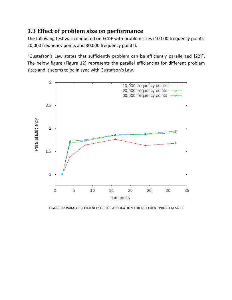
3.3 Effect of problem size on performance The following test was conducted on ECDF with problem sizes (10,000 frequency points,

20,000 frequency points and 30,000 frequency points).

“Gustafson's Law states that sufficiently problem can be efficiently parallelized [22]”.

The below figure (Figure 12) represents the parallel efficiencies for different problem

sizes and it seems to be in sync with Gustafson's Law.

FIGURE 12 PARALLE EFFICIENCIY OF THE APPLICATION FOR DIFFERENT PROBLEM SIZES

3.4 Load Balance The following test was conducted on ECDF with 16 processors and problem size 20,000

frequency points (frequency range from 0Hz to 20Hz with a step size 0.001Hz) and the

code was manually instrumented to determine if there are any load balance issues. The

following table shows that the total number of computations made by each processor in

both frequency domain and time domain is fairly the same and from this it can be

understood that the load is fairly balanced among the processors.

Frequency Domain

Time Domain

Processor Number Tasks handled

Processor Number Tasks handled

8 1110

3 12789

10 1110

6 12936

11 1110

11 12936

14 1110

12 12936

15 1110

13 12936

1 1110

9 12936

2 1110

7 12936

3 1110

2 12985

9 1110

5 12985

4 1110

8 13230

7 1110

10 13279

5 1111

14 13279

6 1115

15 13279

12 1115

1 13279

13 1115

4 13279 TABLE 1: LOAD BALANCE

3.5 Communication overheads The following test was conducted both on Ness and ECDF to determine if there are any

communication overheads and also to determine if they depend on the architecture.

Ness is a pure shared memory system and the communication between the processors

will be very fast where as ECDF is a mixed-structure cluster with 4 processors per node

and communications will not be as fast as in Ness. This Project used Allinea Opt and

Vampirtrace for determination of communication overheads if any present in the

application. The following tests are conducted both on Ness and ECDF with a problem

size of 20,000 frequency points (frequency range from 0Hz to 20Hz with a step size

0.001Hz).

3.5.1 Allinea opt test

FIGURE 13 COMMUNICATION OVERHEAD ANALYSIS ECDF

The above test was carried out on ECDF and the profiling was done using Allinea opt

tool. The existing application implements blocking synchronous send for sending the

tasks to the workers and the workers post a blocking receive to receive the tasks and

these two blocking operations resulted in a late sender situation. In the above figure

(figure 13) it is evident that most of the processors have to wait approximately 3

seconds to receive the task. The above situation is avoided in this project by using non-

blocking communication. This project implemented non-blocking communication and

the mitigated the late sender issue to a considerable extent, the test results of the same

can be found in the performance analysis of new framework.

3.5.2 Vampirtrace analysis

FIGURE 14 COMMUNICATION OVERHEAD ANALYSIS NESS

The above test was carried out on Ness with frequency sample 0HZ - 20Hz and number

of frequency points as 20,000 and the profiling was done using Vampirtrace. From the

above figure (figure 14) it is evident that the application is encountering a late sender

situation at the start, but when compared to the total runtime the time lag is negligible.

Comparing the above two tests we can conclude that the performance loss arising due

communication overheads on systems like Ness (Shared memory) is negligible but it has

a considerable effect on systems like ECDF(mixed architecture).

An overview of the global time line (figure 15) also points out another drawback in the

existing framework. The existing framework’s design is based on taskfarming for both

the phases of computation (frequency domain and time domain). The primary idea of

using a taskfarm is for the sake of adaptive stopping and this is helpful only in the case

of frequency domain computation whereas in the case of time domain adaptive

stopping technique is not being used. With out adaptive stopping there is no need for

the workers to send the results back to the master and sending information which is not

required means a lot of communication overhead. The time taken for computation in

time domain is directly proportional to the number of points present in the time

spectrum and is independent of the position of the point, this means that if the

computation is distributed evenly across the processors then the load will also be evenly

distributed. In the existing framework computational load is distributed only across the

workers and the master stays idle most of the time and also involves unnecessary

communication overhead. In the new framework the time domain computation is not

done using taskfarming instead the work is divided evenly across all the processors, the

design of time domain in the new framework is covered in detail in the next chapter.

FIGURE 15 VAMPIRTRACE GLOBAL TIMELINE

FIGURE 16 OVERALL TIME TAKEN

The above figure (Figure 16) gives an overview of the total time taken for computation

and communication and it can be noted that the total time taken for communication is

19 seconds and where as the time taken for computation is 4min 34 seconds.

A similar test but with frequency sample 0Hz -10Hz and 10,000 frequency points was

run on ECDF with Allinea Opt tracing tool. The following figure (Figure 16) gives an

overview of the time take by each processor for communication and computation.

FIGURE 17COMPUTATION AND COMMUNICATION TIME LINE WITH ALLINEA OPT ON ECDF

From the above figure (Figure 17) it can also be inferred that the load is almost evenly

distributed among the workers and that the time taken for computation by processor

“0” is almost negligible.

3.6 Correctness of Adaptive stopping technique Adaptive stopping technique is based on the assumption that frequencies at the lower

end of the frequency spectrum contribute very little to the time domain solution and a

time domain solution with a considerable accuracy can be attained by curtailing the

frequencies at the lower end of frequency spectrum (explained in 2.2.3 Adaptive

stopping). To ascertain the correctness of our implementation of the adaptive stopping

technique two kinds of tests have been carried out: 1) without adaptive stopping and 2)

with adaptive stopping. Both the above mentioned tests were carried out in frequency

spectrum 0Hz-20Hz. The primary reason for choosing 0Hz – 20Hz frequency sample is

because most of the real time tests are conducted with in the frequency range 0Hz –

10Hz. 0Hz – 20Hz spectrum is an ideal choice because it is neither too small nor it is too

large and also it includes the most commonly used frequency spectrum.

3.6.1 Test 1: Without adaptive stopping

The below test was conducted on ECDF with different problem sizes (by varying the

frequency step) but with same frequency spectrum (0HZ - 20Hz) and adaptive stopping

was switched off. The following figure (Figure 18) is the solution obtained in time

domain (problem size in time domain is same for all the tests) for different problem

sizes in frequency domain. From the following test results it is evident that (with same

sampling spectrum) the solutions appear to overlap with one another irrespective of the

problem size (frequency step size). This means that the solution obtained from the test

with frequency step size “delta frequency = 0.01” (problem size 2,000 frequency points)

completely overlaps with the solution obtained from the test with frequency step size

“delta frequency = 0.001” (problem size 20,000 frequency points). From this test it

appears that the solution obtained for a specific frequency sample is independent of the

frequency step size (delta frequency). The following figure tell us that the solutions are

overlapping completely but it does not say anything about the accuracy of the solution.

The only way to ascertain the accuracy is to find the Pearson’s correlation coefficient

with respect to a known base solution. The following table contains the Pearson’s

correlation coefficients obtained after correlating the time domain solutions of the

above conducted tests with the base solution. The base solution is the solution obtained

for the test case with frequency step size “delta frequency = 0.001” (problem size

20,000 frequency points).

Frequency sample Step size

Number of Frequency points

Pearson's Correlation Coefficient

0 - 20Hz 0.1 200 0.6797049903682510

0 - 20Hz 0.05 400 0.9966668725481230

0 - 20Hz 0.015 1334 0.9999994707644270

0 - 20Hz 0.01 2000 0.9999978974377230

0 - 20Hz 0.005 4000 0.9999995613675370

0 - 20Hz 0.0015 13344 0.9999999930408100

0 - 20Hz 0.001 20000 1.0000000000000000

TABLE 2 COMPARISON OF ACCURACY USING PEARSON'S CORRELATION COEFFICIENT

FIGURE 18: TIME DOMAIN SOLUTIONS FOR DIFFERENT FREQUENCT STEP SIZES

Analyzing the above table (Table 2) and figure (Figure 18) we can come to a conclusion

that the time domain solutions appear to overlap each other for the same frequency

sample with different frequency step sizes. We can also conclude that the accuracy or

resolution of the solution increases as the as the frequency step size decreases. From

the table it is also clear that only a fewer frequency points are required to obtain a

considerably accurate solution.

3.6.2 Test 2: With adaptive stopping

Test similar to the above described test (without adaptive stopping) was carried out

with frequency sample 0Hz – 20Hz and keeping the frequency step size constant for all

the tests but with adaptive stopping switched on. By turning the adaptive stopping on

the computation in frequency domain will stop after the solution in frequency domain

reaches a particular predetermined criteria this means that the computation in

frequency domain will stop in between 0Hz -20Hz depending on the adaptive stopping

criteria. The following figure (Figure 19) is the solutions obtained for the tests carried

out with different adaptive stopping criterion. The test with frequency step size “0.001”

(20,000 frequency points) from the previous tests is taken as the base solution and all

the following tests are compared against this base solution. It is evident from the

following figure (Figure19) that as the number of frequency points increase the tests

reach closer to the base solution. It is also evident from the figure that the test with

18,000 frequency points is notably away from the base solution. The following figure

gives us only visual analysis (qualitative analysis) of the obtained solutions but it fails to

quantify the accuracy of the solution. Pearson’s correlation coefficient test was carried

out to quantify the accuracy of the solutions when compared with the base solution.

FIGURE 19 TIME DOMAIN SOLUTIONS OBTAINED FOR DIFFERENT ADAPTIVE STOPPING CRITERION

Frequency sample Step size

Number of Frequency points

Pearson's Correlation Coefficient

0 - 2Hz 0.00100 2000 0.8726273152918830

0 - 4.2Hz 0.00100 4290 0.9410931971376210

0 – 6.4Hz 0.00100 6400 0.9650859435134950

0 - 11.3Hz 0.00100 11544 0.9838469390730720

0 - 15Hz 0.00100 15000 0.9949471581913920

0 - 18Hz 0.00100 18000 0.9983987590966230

0 - 20Hz 0.00100 20000 1.0000000000000000

TABLE 3 COMPARISON OF ACCURACY USING PEARSON'S CORRELATION COEFFICIENT

From the previous table (Table 3) and figure (figure 19) it is evident that as the test

frequency sample size approaches the base frequency sample size (0Hz – 20Hz) the

solution of the test in time domain moves closer to the base solution. It can also be

noted that the test with 18,000 frequency points does not overlap with the base

solution and Pearson’s correlation coefficient also confirms the same, that the accuracy

of the solution is not good (0.9983987590966230).

3.6.3 Analysis of Test 1 and Test 2 results

From the above figures (Figure 18 and Figure 19) and the table (Table 4) it is evident

that “Test 1” approaches the solution faster and with better accuracy than “Test 2” with

very fewer frequency points. It can be found in the below table that “Test 1” with just

1334 frequency points reaches the solution much faster and with an accuracy much

higher than that of “Test 2” with 18,000 frequency points.

Test 1 Test 2

Frequency sample

Number of

Frequency points

Pearson's Correlation Coefficient

Frequency sample

Number of Frequency

points

Pearson's Correlation Coefficient

0 - 20Hz 200 0.679704990368251

0 - 2Hz 2000 0.8726273152918830

0 - 20Hz 400 0.996666872548123

0 - 4.2Hz 4290 0.9410931971376210

0 - 20Hz 1334 0.999999470764427

0 - 11.3Hz 11544 0.9838469390730720

0 - 20Hz 4000 0.999999561367537

0 - 15Hz 15000 0.9949471581913920

0 - 20Hz 13344 0.999999993040810

0 - 18Hz 18000 0.9983987590966230

0 - 20Hz 20000 1.000000000000000

0 - 20Hz 20000 1.0000000000000000

TABLE 4 COMPARISON OF TEST 1 AND TEST 2

A closer look at the table points out to the unexpected behavior of the application.

“Test1” with just 1334 frequency points to produces a better solution than “Test2” with

18,000 frequency points. The reason for such a behavior can be understood if we take a

closer look at the adaptive stopping technique and time domain integration. Adaptive

stopping technique is based on the understanding that frequencies at lower end of

spectrum contribute more to time domain solution and frequencies at higher end

contribute less, so by curtailing certain part of the frequency spectrum at the higher end

of the spectrum would still provide us a better solution. Time domain computation is

nothing but the summation of the solutions obtained at all the frequency points. The

solution obtained at a particular frequency point at the lower end of spectrum may be

negligible when compared to the solution obtained at the higher end of the frequency

spectrum, but the accumulated result of all the solutions obtained at the end of

frequency spectrum is not negligible and it is evident from the previous figure (Figure

19) that none of the solutions of the “Test 2” overlap with the solution obtained from

the base solution. The above explanation tells us why “Test 2” does not provide an

accurate solution but it does not explain why “Test 1” gives us an accurate solution for

very less computations in frequency domain. The following are the reasons why “Test 1”

gives us an accurate solution for a few frequency point computations.

Time domain computation is nothing but trapezoidal integration of the solutions

obtained in frequency domain. The accuracy of trapezoidal integration depends on the

following factors: Number of points considered, step size between two consecutive

points and nature of the curve. If the curve is smooth and flat to a considerable extent

then the effect of number of points and step size is negligible. In the case of frequency

domain the curve is smooth and is also flat to a certain extent and this is the reason why

“Test 1” provides a better solution for fewer frequency point computations.

3.7 File IO Both the computation frequency domain computation and time domain computation

end with a solution that is written to a file. The existing framework implemented this file

IO in a serial fashion. Even though the time taken for IO is negligible when compared to

total time of computation this project analyzed the feasibility of parallel IO. Detailed

discussion about parallel IO and its performance is provided in the later chapter.

3.8 Conclusions The analysis of above tests leads us to the following conclusions:

1. Points at the higher end of frequency spectrum contribute little to the time

domain solution when compared to the points at the lower end but it is not

negligible enough to be neglected.

2. Considerably accurate solution can be attained with fewer frequencies.

3. The application reaches the solution faster with a higher accuracy if it covers the

entire frequency spectrum (test 1) instead of skipping certain part of the

frequency spectrum it is the case in adaptive stopping (test 2).

4. The existing framework with the adaptive stopping is not producing accurate

results because of the way the technique is implemented. According to adaptive

stopping technique as soon the frequency domain computation reaches a

threshold the computation is stopped and the rest of the frequency spectrum is

curtailed and curtailing a part of the spectrum would mean loss of accuracy. This

project tried to fix the defect and implement adaptive stopping technique, but

this framework is designed in such a way that it is not possible to implement

adaptive stopping technique. Details regarding the adaptive stopping technique

are discussed in future aspects chapter.

5. In time domain computation taskfarming leads to unnecessary communication

overheads and load imbalance.

Chapter 4

4.1 Frequency domain computation

4.1.1 Objective

The deciding factor in the performance of the CSEM application is the number of

frequency points computed, the lesser the number of frequency points computed the

better the performance.

The primary objective of this project is to provide a solution with considerable accuracy

and also to improve the performance of the application.

Keeping in mind the conclusions from the previous chapter this project tries to strike a

balance between application performance and accuracy of the solution. It is understood

that frequencies at the lower end of spectrum contribute more to the solution than that

of the frequencies at the higher end but at the same time we can not neglect the

frequencies at the higher end of spectrum completely.

A closer look at the figure (Figure 3 Frequency Domain Solution) indicates that the

gradient of the frequency domain solution is negative most of the part of the curve and

gradually reaches zero as it reaches the end of the spectrum. It is understood that the

error of integration in trapezoidal integration is minimal or negligible for nearly flat

curves even with bigger step sizes. The implementation of Adaptive frequency step size

is based on this concept. Having a smaller step size at the start of the frequency

spectrum and gradually increasing the step size as the computation reaches the higher

end of the spectrum a solution with reasonable accuracy can be obtained.

4.1.2 Design

Frequency domain computation in the new framework consists of two main

components taskfarm and adaptive frequency step technique. The new framework is

similar to that of the existing framework but with the following differences.

1. Since the frequency step size is constant through out the computation the

existing frame work is completely based on the starting point and stopping point

of the frequency domain computation. Where as in the new framework the

frequency step size varies from task to task and for this reason the new

framework is completely redesigned and is now based on start frequency and

stop frequency.

2. In the existing framework the elements of a task are starting point and stopping

point which decides the start and the end points of frequency domain

computation for that task. The new frame work consists of start frequency it tells

the worker the starting frequency in the frequency domain computation, task

size it decides the size of each task and delta frequency it tells the frequency step

size of each task.

3. The adaptive stopping technique is implemented in such a way that the

computation in frequency domain stops when the solution reaches a particular

stopping criteria and after this, rest of the frequencies are completely neglected.

In the new framework when the solution reaches the stopping criteria, similar to

the existing framework the computation is stopped, but instead of completely

neglecting the solutions of the rest of the frequencies the application assumes

the solution of the neglected frequencies to be the same as the solution of the

last computed frequency.

The following pseudo code gives an overview of the taskfarm in the new framework:

The main elements of a task in the new framework are:

1) Start frequency (tells the starting frequency for the computation of the task).

2) Task size (Tells the number of frequency points that are to computed).

3) Step size (frequency step size)

Master

Start Do loop o Check if the computation reached the end frequency point, if yes then quit

computation. o Wait for results from workers. o Call adaptive frequency step subroutine and create a new task. o Send out the new task to the worker from which the latest result was

received. End loop Close the taskfarm by sending termination signal to all the workers.

Worker

Complete the first set of tasks. Start Do loop Wait for the tasks from the master.

o If task received is a termination signal exit the loop. o Start loop (Start frequency to end frequency)

Do the frequency domain computation. Send the gradients of the solution to the master.

o End loop End Do loop.

The worker does not return the entire solution to the master instead it just sends back

the information about the changing rate of the amplitude “gradient1”, “gradient2” and

“gradient”. Where “gradient1”, “gradient2” and “gradient” are the gradients of the first

half, second half and the full curve respectively of the most recently computed task. The

primary idea behind sending the gradient is to check the flatness of the curve.

Adaptive frequency step

The key idea behind this technique is to increase the frequency step size adaptively as

the computation proceeds from lower end of the frequency spectrum to the higher end.

The following steps give a brief overview of this technique.

1. Check the gradients “gradient1”, “gradient2” and “gradient” obtained from the

latest result and verify if they are negative. This step makes sure that curve is

monotonically decreasing.

2. Check if “gradient” (changing rate of the full task) is less than a predefined

threshold.

3. If the above two conditions are met then we can assume that the curve is

progressing smoothly. Increment the counter by one.

4. If the counter reaches a particular depth then increase frequency step size by a

factor. The reason for including this step is to make sure that the curve is flat and

smooth.

5. Decrement the task size by a factor. The size of the task is inversely proportional

to the number of communications made. In a many tests it has been found that

adaptive frequency step technique comes into play only after a certain point in

the frequency spectrum and with smaller task sizes the application does a lot of

unnecessary communications among the processors. This unnecessary

communication can be avoided by using an optimum task size.

6. If step 1 and step 2 fail then check if any of “gradient1”, “gradient2” and

“gradient” is greater than or equal to zero. If at least one of the gradients is

greater than zero then reset the frequency step size to the initial step size. This

step makes sure that a larger step size is not used if the computation encounters

spikes.

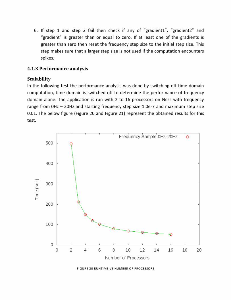
4.1.3 Performance analysis

Scalability

In the following test the performance analysis was done by switching off time domain

computation, time domain is switched off to determine the performance of frequency

domain alone. The application is run with 2 to 16 processors on Ness with frequency

range from 0Hz – 20Hz and starting frequency step size 1.0e-7 and maximum step size

0.01. The below figure (Figure 20 and Figure 21) represent the obtained results for this

test.

FIGURE 20 RUNTIME VS NUMBER OF PROCESSORS

FIGURE 21 PARALEL EFFICIENCY OF NEW FRAMEWORK

From the above figure (Figure 20 and Figure 21) it is clear and evident that the runtime

decreases as the number of processors increase. It can also be noted that the

performance behavior of the new framework is similar to the existing framework which

is discussed in chapter 3(3.2 Scalability)

To verify if there is any change in the behavior of the framework the project tested the

framework with three different problem sizes 1) 0Hz -4 Hz 2) 0Hz -20Hz and 3)0Hz –

40Hz. The following figure (Figure 22) is the outcome of these tests. It is clear from this

figure that the performance behavior of is the same as the existing framework. Though

the performance behaviors look the same only an actual comparison between the

obtained results can explain the performance improvement, which is discussed later in

this chapter.

FIGURE 22 COMPARISON RUNTIMES FOR DIFFERENT PROBLEM SIZES

Load Balance

The following test was carried on 16 processors (in ECDF) with frequency sample 0Hz –

20Hz, starting frequency step size “1.0e-06” and maximum frequency step size as

“0.01”. The code was manually instrumented to determine the number of points

computed. The following table gives the test results.

Processor rank Number of

Computations Processor

rank Number of

Computations

1 500 8 500

2 505 9 505

3 500 10 505

4 505 11 505

5 505 12 502

6 503 13 505

7 505 14 505

15 505

TABLE 5 LOAD BALANCE IN NEW FRAMEWORK

The above results clearly indicate that the load is almost evenly balanced among all the

workers of the taskfarm.

Factors affecting performance and accuracy of the new framework

The primary components of the technique that would affect the accuracy and

performance of the application are,

1) Starting frequency step size

2) Maximum frequency step size

3) Task size (Determines the number of frequency points in a task)

4) Delta factor (Rate at which the frequency step size is incremented.).

A series of tests were conducted to determine the optimum combination of the above

elements.

Impact of “frequency step size” on performance

Unlike the existing framework which has a constant step size, the new framework has a

variable step size. The frequency step size depends upon all the above mentioned

elements. To strike a balance between accuracy and performance the above mentioned

elements should be set to optimal value. The optimal value of these elements varies

from problem to problem because they are mainly dependent on the nature of the

solution as well. This project tried to attain the optimum values for these elements by a

series of hit and trail methods, of which results of some of them are given below.

The following tests were conducted on Ness in frequency spectrum 0Hz – 20Hz.

The solution obtained from the existing framework with a frequency spectrum 0Hz –

20Hz and 40,000 frequency points is considered as the base solution. The solutions

obtained from the test cases are compared against this base solution.

The following process is followed to determine reasonable values of the above

mentioned elements:

Step 1: The application is run with different combinations of “Start frequency step size”

and “End frequency step size” and the obtained solutions(time domain) are compared

with the base solution using Pearson’s correlation and among these the combination

which offers a better balance of performance and accuracy is considered.

Step 2: After obtaining a reasonably good value of “Start and End frequency step sizes”

the application is tested with different task sizes and a the obtained solutions(time

domain) are compared with the base solution using Pearson’s correlation and among

these the task size which offers a reasonable accuracy and better performance is

considered.

Step 3: delta factor is determined in a similar fashion as mentioned above steps.

Step 1:

The following tests are run with varying combinations of frequency step sizes as

mentioned in the table.

Start Step size

End step size

Pearson's Correlation Coefficient

Time Taken(Sec)

1.00E-07 1.00E-01 0.84719199826043 51.17234

1.00E-07 1.00E-02 0.99999631710031 66.35270405

1.00E-07 1.00E-03 0.99999999548880 297.268676

1.00E-06 1.00E-02 0.99999239470466 64.75868416

1.00E-06 1.00E-03 0.99999996646159 299.0754542

1.00E-05 1.00E-02 0.99999593841666 64.47768211

1.00E-05 1.00E-03 0.99999996674902 331.3323638

1.00E-08 1.00E-02 0.99999504978661 77.31186986

TABLE 6 OPTIMUM START STEP SIZE AND END STEP SIZE COMBINATION

From the above table (Table 6) we can derive the following conclusions:

1) A Smaller change in the end step size improves the accuracy to a grater extent but at

the same time the computational time also increases in to far grater extent.

2) The effect of start frequency step size appears to be fairly constant.

3) From the above table we can assume that the combination with start frequency step

size as 1.0E-7 and end frequency step size 1.0E-2 offers a reasonable accuracy and

better performance as well.

Step 2

The following tests are run with varying task sizes.

Task size

Pearson's Correlation Coefficient

Time Taken(Sec)

7 0.9999961037129 31.12602782

10 0.9999961207856 31.72712207

30 0.9999961942123 42.51087189

50 0.9999962076978 50.35472798

100 0.9999963171003 66.35270405

150 0.9999964255876 92.34237194 TABLE 7 DETERMINATION OF OPTIMUM TASK SIZE

From the above table it is evident that the optimum task size is “10”.

Step 3

The following tests are run with different delta factors.

Delta factor

Pearson's Correlation Coefficient

Time Taken(Sec)

1.2 0.999996507856330 33.84768009

1.5 0.999995414028554 33.54673004

2 0.999996144694599 30.51572704

3 0.999993452728071 32.58413506 TABLE 8 DETERMINATION OF OPTIMUM DELTA FACTOR

From the above table we can conclude that delta factor as “1.2” provides considerable

accuracy and reasonable performance.

From the above tests we can conclude that a good balance between performance and

accuracy with the following values for the above mentioned elements:

1) Starting frequency step size =1.0E-07

2) Maximum frequency step size =1.0E-02

3) Task size = 10

4) Delta factor =1.2

4.2 Time Domain Integration After obtaining the solution in frequency domain the application performs a trapezoidal

integration on the frequency domain solution to provide a solution in time domain.

Drawbacks of the existing framework

The existing framework utilizes taskfarming for time domain computation, but the

primary reason for implementing taskfarming is for adaptive stopping in frequency

domain computation. Utilizing taskfarming for time domain computation would mean

extra communication over head and also the master processor stays idle through out

computation.

Keeping in mind the drawbacks of the existing framework, this project tries to overcome

those drawbacks by redesigning time domain computation framework.

4.2.1 Design 1. Divide the time domain spectrum into ‘n’ tasks where ‘n’ is the number of

processors.

2. Each processor does the time integration for one task.

3. Root processor gathers the solution from all the processors.

4. Write the solution to a file.

The existing project implemented the implemented the time domain integration using a

simple trapezoidal integration technique (2.2.3 Time Domain Computation). This project

implemented three different integration schemes and also investigated the

performance and accuracy of these integration schemes.

The primary goal of the integration schemes is to find the integral of a function

tabulated at unequally spaced data points and three different integration schemes are

investigated to achieve this goal.

1) Overlapping polynomials

2) 3 point Lagrangian interpolation

3) Trapezoidal integration of unequally spaced data.

Overlapping parabolas technique:

This integrating scheme is based on overlapping parabolas [23].

It is understood that for a set of three different points (‘x1’, ‘x 2’, ‘x3’) there exists a

quadratic polynomial that passes through the three points and it can be represented as,

𝑓𝑖 𝑥𝑖−1, 𝑥𝑖 , 𝑥𝑖+1 = 𝑎𝑖𝑥2 + 𝑏𝑖𝑥 + 𝑐𝑖

The idea behind this technique can be understood from the below figure (Figure 23).

FIGURE 23 OVERLAPPING PARABOLAS

The above figure represents two parabolas Curve-1 and Curve-1 passing through three

points 𝑥𝑖−1, 𝑥𝑖 , 𝑥𝑖+1 and 𝑥𝑖 , 𝑥𝑖+1, 𝑥𝑖+2 respectively. The area between the points

𝑥𝑖 , 𝑥𝑖+1 is the average of the area between the two mentioned points for both the

curves.

The area between the two points 𝑥𝑖 , 𝑥𝑖+1 can be obtained by following the below

integration step.

𝑓 𝑥 = 12 𝑓 𝑥𝑖−1, 𝑥𝑖 , 𝑥𝑖+1

𝑥𝑖+1

𝑥𝑖

+ 𝑓 𝑥𝑖 , 𝑥𝑖+1, 𝑥𝑖+2 𝑥𝑖+1

𝑥𝑖

𝑥𝑖+1

𝑥𝑖

Curve-1

Curve-1

𝑥𝑖−1 𝑥𝑖 𝑥𝑖+1 𝑥𝑖+2

The above integration step is followed for ‘i’ values lying between (2 and n-1) for the

area between points (1,2) and (n-1,n) is calculated by using only a single curve instead

of averaging between two curves (‘n’ is the number of frequency points).

3 Point Lagrangian interpolation

This integration scheme is based on 3 – Point Lagrangian interpolation. It is understood

that there exists a polynomial of degree ‘n’ ‘P(x)’ for a set of ‘n+1’ distinct points and it

can be obtained from the below formula [23]:

𝑃 𝑥 = 𝑥 − 𝑥𝑖

𝑥𝑗 − 𝑥𝑖

× 𝑦𝑗

𝑛

𝑖=0,𝑖<>𝑗

𝑊𝑕𝑒𝑟𝑒 𝑦𝑗 = 𝑃 𝑥𝑖

A brief overview of the integration process:

Set the result to ‘0’.

Start the Do loop

o Determine the coefficients of the quadratic polynomial ‘P(x)’ for a set of

three points.

o Integrate the area under the polynomial in between the points.

o Add the obtained value to the result.

End the loop.

Trapezoidal integration of unequally spaced data:

The existing framework uses trapezoidal integration scheme for integration of solution

obtained in frequency domain. Since the frequency step size is constant through out the

frequency domain the same integration scheme can not be used in the new framework.

The existing framework modified the trapezoidal integration technique so that it can be

applied to unequally spaced data.

The following pseudo code gives a brief overview of the technique:

𝑟𝑒𝑠𝑢𝑙𝑡 = 0

Start Do loop

∆ = 𝑥𝑖+1 − 𝑥𝑖

𝑟𝑒𝑠𝑢𝑙𝑡 = 𝑟𝑒𝑠𝑢𝑙𝑡 + ∆ 𝑓 𝑥𝑖 + 𝑓 𝑥𝑖+1

End loop

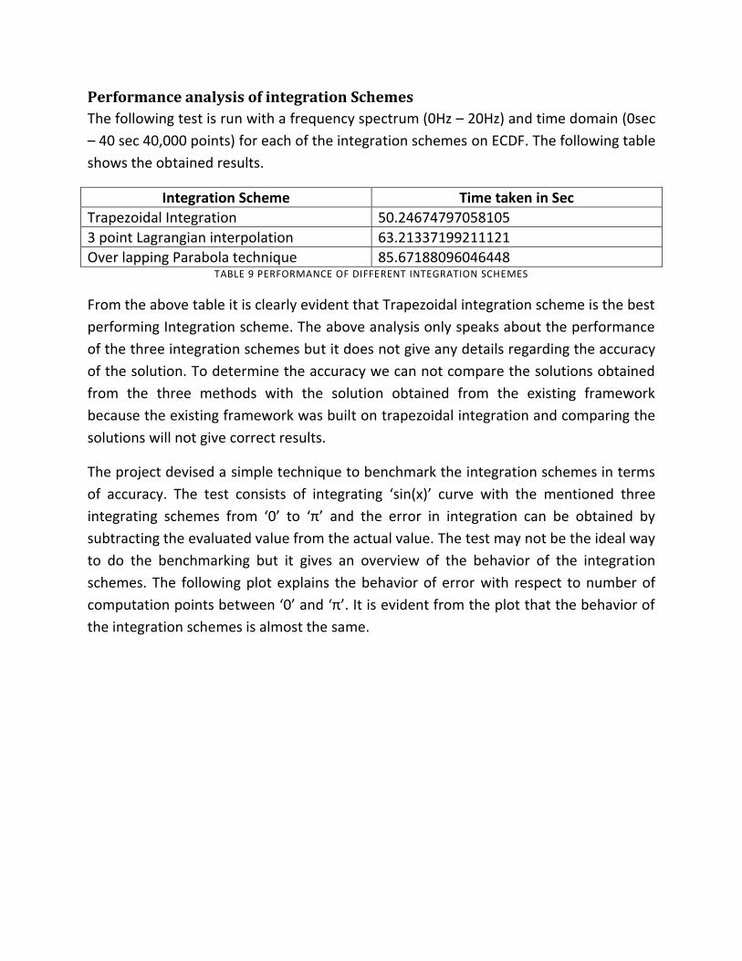
Performance analysis of integration Schemes

The following test is run with a frequency spectrum (0Hz – 20Hz) and time domain (0sec

– 40 sec 40,000 points) for each of the integration schemes on ECDF. The following table

shows the obtained results.

Integration Scheme Time taken in Sec

Trapezoidal Integration 50.24674797058105

3 point Lagrangian interpolation 63.21337199211121

Over lapping Parabola technique 85.67188096046448 TABLE 9 PERFORMANCE OF DIFFERENT INTEGRATION SCHEMES

From the above table it is clearly evident that Trapezoidal integration scheme is the best

performing Integration scheme. The above analysis only speaks about the performance

of the three integration schemes but it does not give any details regarding the accuracy

of the solution. To determine the accuracy we can not compare the solutions obtained

from the three methods with the solution obtained from the existing framework

because the existing framework was built on trapezoidal integration and comparing the

solutions will not give correct results.

The project devised a simple technique to benchmark the integration schemes in terms

of accuracy. The test consists of integrating ‘sin(x)’ curve with the mentioned three

integrating schemes from ‘0’ to ‘π’ and the error in integration can be obtained by

subtracting the evaluated value from the actual value. The test may not be the ideal way

to do the benchmarking but it gives an overview of the behavior of the integration

schemes. The following plot explains the behavior of error with respect to number of

computation points between ‘0’ and ‘π’. It is evident from the plot that the behavior of

the integration schemes is almost the same.

FIGURE 24 ERROR OF INTEGRATION IN DIFFERENT INTEGRATION SCHEMES

From the above figure(Figure 24) and table (Table 9) we can conclude that Trapezoidal

integration performs better and is reasonably accurate.

The drawback of this test is that function considered (sine) is a smooth function, but in

situations where the data is not smooth and has a lot of spikes then the error

trapezoidal integration might be considerably higher than the others.

4.2.2 Load balance

The new framework is designed in such way that the load is balance implicitly. The

following test was run on 16 processors with frequency sample (0Hz – 20Hz) and time

domain (0sec – 40 sec 40,000 points) on ECDF with trapezoidal integration scheme as

the underlying integration technique.

Processor Number

Runtime (Sec)

Processor Number

Runtime (Sec)

1 50.08821392 9 50.24674797

2 50.15579295 10 50.16054893

3 50.22439003 11 50.2089231

4 50.18649697 12 50.18569207

5 50.22098684 13 50.20796895

6 50.18644118 14 50.24039316

7 50.1780479 15 50.21508384

8 50.21760201 16 50.18391585 TABLE 10 LOAD BALANCE TIME DOMAIN COMPUTATION

From the above table we can conclude that the load among the processors in time

domain computation is perfectly balanced.

4.3 File IO

After the completion of the computation in both frequency domain and time domain

the solution is written to a file. In the existing framework the file IO is handled in a serial

fashion. The new framework implemented two different types of file IO,

1. Serial IO with netCDF4.

2. Parallel IO with HDF5.

The following steps illustrate the basic structure of the code in HDF5:

1) Initialize HDF5.

2) Setup file access property as parallel access.

3) Collectively open a file, this step returns a file handle for future use.

4) Create a dataset with default properties include data type etc. This step returns a

handle for the dataset. (Dataset is an array)

5) Define the location in file where the data needs to be written.

6) Write the dataset collectively.

7) Close HDF5.

The following steps illustrate the basic structure of the code in netCDF4:

1) Open a file. This step returns a file handle for future access.

2) Define the dimensions. This step includes defining dimensions by giving them

names, length of the dimension and this step returns a dimension id. In our

project we have three arrays so three dimensions (one dimension for each

array).

3) Define the datasets. This step includes defining the three arrays and it will

return a dataset id for each array.

4) Select the chunk of data from memory.

5) Write to netCDF file.

6) Close netCDF.

Performance Analysis of HDF5 Parallel IO

The Parallel IO is tested with different sizes of input array (number of points in

frequency spectrum) and the following are the results:

File size(number of lines) Serial IO (sec) Parallel IO (sec) 8 Processors

100 9.9998E-4 0.114

10000 6.499E-2 0.152

100000 0.6599 0.91487

3000000 2.018976 2.257657 TABLE 11 PARALLEL IO HDF5 PERFORMANCE

Performance analysis of netCDF4 Serial IO

The netCDF4 serial IO test was carried out on ECDF with time spectrum 0 to 20 seconds

(200,000 points) and the following are the results.

File size(number of lines) Serial IO netCDF4 Serial IO

20,0000 1.4798234 17.15320978 TABLE 12 NETCDF4 SERIAL IO PERFORMANCE

From the above tables (Table11 and Table 12) it is evident both HDF5 parallel IO and

netCDF4 serial IO are not performing. Following are the reasons for poor performance

of both the libraries:

1) Startup cost, both netCDF4 and HDF5 start with initialization.

2) Most of the calls in both netCDF4 and HDF5 are collective and there can be

synchronization issues.

3) HDF5 includes data compression, it does data compression with the help zlib or

szlib and this acts as another overhead.

4) It can be noted from table 11 that for the array size of just 100 HDF5 tale 0.11

seconds where system IO is of the order 1.0E-4, this clearly points overheads in

HDF5.

5) Table 11 also points that as the problem size increases (number of lines

increases) HDF5 tries to performance. From this we can infer that HDF5 is not

suitable for small sized data.

4.4 Performance comparison of new framework with existing

framework

Comparison of the frequency domain solution

The primary goal of this project is to improve the accuracy of the solution by solving

more frequencies at the lower end of spectrum than at higher end. The following figure

(Figure 25) is the frequency domain solution obtained by the new framework. By

comparing the figure (Figure 25) and figure (Figure 26) we can clearly see that the

primary goal of the project is achieved.

FIGURE 25FREQUENCY DOMAIN SOLUTION NEW FRAMEWORK

The above figure (Figure 25) consists of three parts:

Part 1) Frequency step size is the minimum.

Part 2) Frequency step size starts increasing.

Part 3) Frequency step size reaches maximum step size value and remains constant.

The following figure is the frequency domain solution obtained by the existing

framework,

Part 1

Part 2

Part 3

A

m

p

l

i

t

u

d

e

Frequency

Frequency Domain

Solution

FIGURE 26 FREQUENCY DOMAIN SOLUTION EXISTING FRAMEWORK

Comparing the above two figures (Figure 25 and Figure 26) we can clearly point out the

differences between the existing framework and the new framework. It is evident from

the figures that the new framework does more computation at the lower end of the

spectrum than at the higher end.

Frequency

A

m

p

l

i

t

u

d

e

Frequency

Domain Solution

Existing

Framework

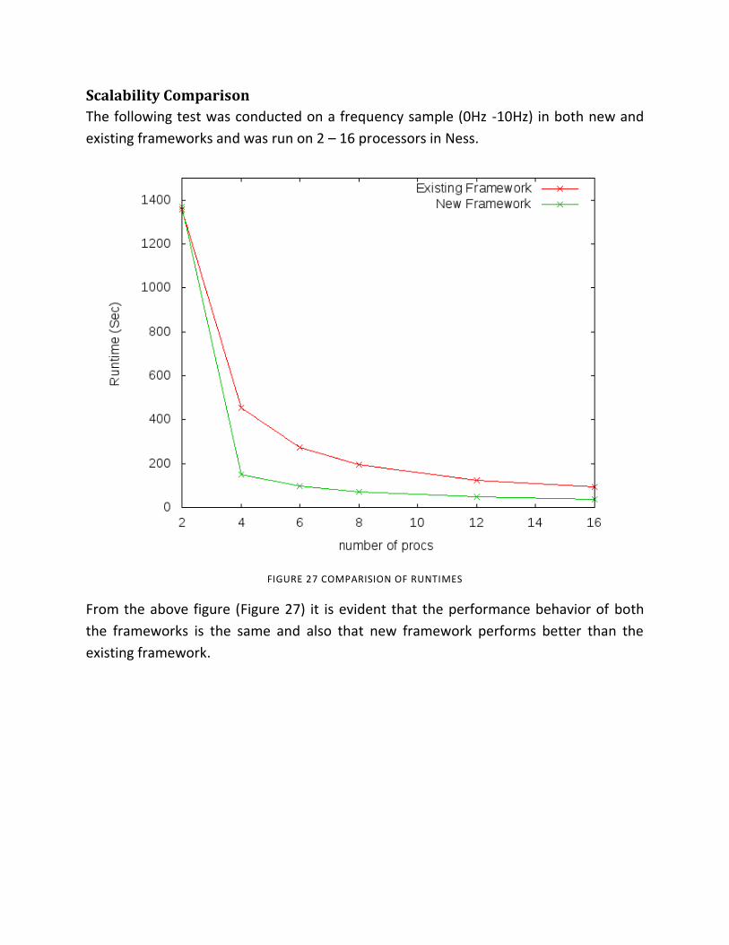
Scalability Comparison

The following test was conducted on a frequency sample (0Hz -10Hz) in both new and

existing frameworks and was run on 2 – 16 processors in Ness.

FIGURE 27 COMPARISION OF RUNTIMES

From the above figure (Figure 27) it is evident that the performance behavior of both

the frameworks is the same and also that new framework performs better than the

existing framework.

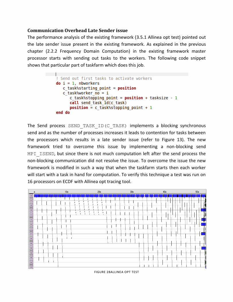
Communication Overhead Late Sender issue

The performance analysis of the existing framework (3.5.1 Allinea opt test) pointed out

the late sender issue present in the existing framework. As explained in the previous

chapter (2.2.2 Frequency Domain Computation) in the existing framework master

processor starts with sending out tasks to the workers. The following code snippet

shows that particular part of taskfarm which does this job.

The Send process SEND_TASK_ID(C_TASK) implements a blocking synchronous

send and as the number of processes increases it leads to contention for tasks between

the processors which results in a late sender issue (refer to Figure 13). The new

framework tried to overcome this issue by implementing a non-blocking send

MPI_ISEND, but since there is not much computation left after the send process the

non-blocking communication did not resolve the issue. To overcome the issue the new

framework is modified in such a way that when the taskfarm starts then each worker

will start with a task in hand for computation. To verify this technique a test was run on

16 processors on ECDF with Allinea opt tracing tool.

FIGURE 28ALLINEA OPT TEST

Communication overhead in time domain

In the previous chapter (3.5.2 Vampirtrace analysis) the performance analysis of the

existing code pointed out communication overheads in time domain computation due

to the implementation of taskfarming in time domain. Time domain computation in the

new framework is designed in such a fashion that the amount of communication will be

minimum. A test was run on Ness with time spectrum 0 – 40 seconds and number of

time points 40,000 to verify the same.

Comparing the below figure (Figure 29) and Figure 15 it clearly shows the reduced

amount of communication in time domain.

FIGURE 29 VAMPIRTRACE GLOBAL TIME LINE NEW FRAMEWORK

Runtime vs Accuracy

The following test was conducted on Ness with frequency spectrum 0Hz to 20Hz and

time spectrum 0 seconds to 40 seconds (40,000 points) and the solution is then

compared solution obtained in the existing framework existing framework with the

same frequency spectrum and 40,000 frequency points.

The existing framework took 367.86521 seconds for the computation.

Start Step size End step size

Pearson's Correlation Time

Taken(Sec) Speedup Coefficient

1.00E-07 1.00E-01 0.847191998 51.172 718.88

1.00E-07 1.00E-02 0.999996317 66.353 554.41

1.00E-07 1.00E-03 0.999999995 297.27 123.75

1.00E-06 1.00E-02 0.999992395 64.759 568.06

1.00E-06 1.00E-03 0.999999966 299.08 123

1.00E-05 1.00E-02 0.999995938 64.478 570.53

1.00E-05 1.00E-03 0.999999967 331.33 111.03

1.00E-08 1.00E-02 0.99999505 77.312 475.82 TABLE 13 RUNTIME VS ACCURACY

From the above table we can conclude that depending upon the accuracy of the

solution the sppedup gain of the new framework when compared with the original

framework is between 475% to 568%.

Chapter 5

Conclusions and Future work

5.1 Conclusions The project successfully implemented adaptive frequency step size in the new

framework. For specific problems the performance gain obtained by implementing this

technique is in the range of 475% to 568%.

The project also investigated the feasibility of different integration schemes and came to

a conclusion that Trapezoidal integration gives a good performance and accuracy for

time domain integration.

The project investigated and implemented parallel HDF5 and serial netCDF4 and came

to the conclusion that it may not provide the expected performance for 1D-kernel.

5.2 Future work Due to time limit the project is unable to investigate some of the techniques that may

improve the performance of the application.

Adaptive Stopping technique

The existing framework implemented adaptive stopping technique, but while analyzing

the performance of the application this project found a bug in the implementation of

adaptive stopping technique. According to the existing logic after the solution reaches a

particular threshold in the frequency domain the technique stops the application and

neglects the solutions of the rest of the frequency spectrum. The solution at each

frequency point may be negligible but neglecting a part of the spectrum makes the

solution to deviate from the actual solution.

Solution

The possible way of correcting this defect is to copy the solution of the last computed

frequency point to the rest of the spectrum.

Factors inhibiting the implementation of adaptive stopping in new framework

Since at any given point of time ‘n’ number of workers will be doing the frequency

domain computation and since the project implements adaptive frequency step size

technique it is highly unlikely that all the workers will be working with the same number

of frequency points (the problem sizes will be different), which means that the last

arrived solution may not be the last frequency point of the computed spectrum. Copying

anything other than the solution of the last computed frequency point to the neglected

spectrum will result in totally wrong solution in time domain.

Parallel netCDF4

One of the draw backs of the new framework is that, the total number of frequency

points to be computed is not known during the start of the framework and the arrays

are allocated to an assumed size in the start of computation. Allocating array with sizes

more than what is required will result in poor performance and allocating arrays with

sizes less than what is actually required will result in abrupt stopping of the

computation.

Parallel netCDF4 comes with a feature called “UNLIMITED” dimension in which a dataset

(array) can have a dimension to unlimited size. Converting all the arrays to netCDF4

datasets will help in resolving the array size issue, but the performance aspect

associated with it needs to be analyzed.

Porting the code to higher kernels

The actual runtime of the application is hardly couple of minutes, the primary reason for

implementing this new framework is to understand how higher kernels (2D, 2.5D and

3D) might behave with a similar framework, but an actual implementation will only tell

us the pitfalls or overheads associated with this framework.

Bibliography 1. Introduction to Marine Exploration. [Online]

http://www.dmtcalaska.org/exploration/ISU/intro.html.

2. A Framework for Parallelising a Controlled Source Electro Magnetic Code. Deng, Yi.

2008.

3. OHM weblink. [Online] http://www.ohmsurveys.com/.

4. The Leading Edge; April 2006; v. 25; no. 4; p. 438-444. Constable, Steven.

5. Marine Controlled-Source Electromagnetic Methods GEOPHYSICS vol72. Constable,

Steven.

6. Marine time domain CSEM: an emerging technology. Allegar, Kurt Strack and

Norman. SEG Annual Meeting, Las Vegas : s.n., 2008.

7. 2D Marine controlled-source electro magnetic. Yuguo Li, Steven Constable. 2007,

GEOPHYSICS vol72.

8. Stat oil. [Online] www.statoil.co.uk.

9. Exxon mobil. [Online] www.exxonmobil.co.uk.

10. Netcdf. [Online] www.unidata.ucar.edu/software/netcdf/.

11. netcdf. netcdf FAQ. [Online]

http://www.unidata.ucar.edu/software/netcdf/docs/faq.html#whatisit.

12. netCDF users guide. netCDF users guide. [Online]

http://www.ipp.mpg.de/~dpc/netcdf_guide/guide_91.html.

13. netcdf wiki. [Online] http://en.wikipedia.org/wiki/NetCDF#Format_description.

14. HDF5 web link. [Online] http://www.hdfgroup.org/.

15. HDF datasets. [Online] http://www.hdfgroup.org/HDF5/doc/H5.intro.html#Intro-

FileOrg.

16. Vampirtrace installation and User guide. Germany : Pallas Gmbh.

17. Allinea Opt. [Online] http://www.allinea.com/?page=74.

18. Person's correlation coefficient. [Online]

http://hsc.uwe.ac.uk/dataanalysis/quantInfAssPear.asp.

19. Ness Website. [Online]

http://www2.epcc.ed.ac.uk/~ness/documentation/ness/index.html.

20. ECDF website. [Online] http://www.ecdf.ed.ac.uk/.

21. Amdahl's law. [Online] http://en.wikipedia.org/wiki/Amdahl's_law.

22. Gustafson's Law. [Online] http://en.wikipedia.org/wiki/Gustafson's_law.

23. Marine Controlled-Source Electromagnetic Methods GEOPHYSICS vol72. Constable,

Steven.