Optimizers for single and multi-stage job-shop scheduling ...

AN ABSTRACT OF THE THESIS OF

PANCHATCHARAM RAMALINGAM for the MASTER OF SCIENCE (Name (Degree)

in INDUSTRIAL ENGINEERING presented on .14 8 /9 (Major) (Date)

Title: OPTIMIZERS FOR SINGLE AND MULTI -STAGE JOB -SHOP

SCHEDULING P OBLE S

Abstract approved: r. Michael S. Inoue

Scheduling, an important function of any industrial operations

control system, specifies the precise use of production facilities at

each instant of time.

This paper summarizes numerous computational methods and

objective functions applicable to a wide variety of manufacturing situ-

ations. Both single -stage problems, with and without setup times,

and multi -stage problems are examined.

A linear programming model is formulated for determining an

optimal schedule that minimizes the makespan for processing n

jobs on m 'not -alike' single -stage facilities. An open -path sched-

uling algorithm has also been developed and described in this paper as

an application of the branch and bound technique for scheduling a set

of non - repetitive jobs on a single -stage processor.

Numerical examples are used throughout the paper to illustrate

the algorithms for various optimizers.

Optimizers for Single and Multi -Stage Job -Shop Scheduling Problems

by

Panchatcharam Ramalingam

A THESIS

submitted to

Oregon State University

in partial fulfillment of the requirements for the

degree of

Master of Science

June 1969

APPROVED:

Assdciate Professor of Industrial Engineering

in charge of major

Head of epartment of Indu t ial Engineering

Dean of Graduate School

Date thesis is presented

Typed by Clover Redfern for Panchatcharam Ramalingam

/i (9 CGL

ACKNOWLEDGMENT

I am deeply indebted to Dr. Michael S. Inoue for his most help-

ful advice, guidance and unfailing help during my graduate work and

the course of this investigation.

I would also like to express my sincere appreciation and thanks

to Dr. James L. Riggs for his personal encouragement throughout

my graduate work.

The academic assistance and help from Dr. Donald A. Pierce,

Dr. Donald Guthrie and Dr. V. J. Bowman, Jr. of the Statistics

Department and Professor William F. Engesser of the Department of

Industrial Engineering is gratefully acknowledged. Thanks are also

due to many of the authors referred in the bibliography for permis-

sion to include their work in this thesis.

Finally, I wish to express my appreciation to Mrs. Redfern for

her superb job of typing the final copy and to Type -Ink for sustaining

cheerfully the multiple pressures for meeting the deadlines.

TABLE OF CONTENTS

Chapter

I. INTRODUCTION

Page

1

II. SINGLE STAGE -SETUP TIME INCLUDED WITH PROCESSING TIME 5

A. Tardiness 7

1. Maximum Tardiness of the Jobs 7

B. Completion Times 11

1. Sum of Completion Times 12

2. Weighted Sum of Completion Times 21

C. Penalty Cost 28

1. Linear Loss Function 29

2. Non - Linear Loss Function 37

D. Elapsed Time -- Scheduling on 'Not- Alike' Processors 49

1. Three Jobs on Two Processors 50

2. A Linear Programming Model 56

III. SINGLE STAGE - -SETUP TIME SEPARATED FROM PROCESSING TIME 63

A. Elapsed Time 63

1. A Set of Repetitive Jobs -- Travelling Salesman Problem (Closed Path Scheduling) 65

2. A Set of Non -Repetitive Jobs 77

(a) Heuristic Rules. 77

(b) Application of Branch and Bound Technique 81

IV. TWO -STAGES- -SETUP TIMES INCLUDED WITH PROCESSING TIMES 90 A. Completion Times - -Sum of Completion Times 90

B. Elapsed Time 97

1. Johnson's Method 98

2. Start and Stop Timelags 102

3. Generalized Johnson's Rule for Job -Lots 110

V. THREE STAGES- -SETUP TIME INCLUDED WITH PROCESSING TIME A. Elapsed Time

1. Johnson's Rule (a Restricted Case) 2. Computational Methods by Giglo and Wagner

114 114 114 117

-

Chapter Page

VI. M- STAGES- -SETUP TIME INCLUDED WITH PROCESSING TIME 122 A. Tardiness 123

1. Total Tardiness Over All Jobs 123 B. Elapsed Time 136

1. Combinational Analysis 136 (a) Matrix Method. 136

Open Scheduling Problem 142 Dual -Open Scheduling Problem 148 Mixed Scheduling Problem 154

(b) Linear and Monte Carlo Algorithms 154 (c) Application of Branch and Bound Technique 161

Algorithm by Brooks and White 161 Algorithm by Ignall and Schrage 176

(d) Algorithm by Dudek and Teuton 183 2. Graphical Algorithm 194 3. Programming Methods 203

(a) Linear Programming Model 203 (b) Integer Linear Programming Models 208

Algorithm by Bowman 208 Algorithm by Manne 215 Algorithm by Wagner 218

C. Total Cost (Production and Storage Cost) 221 1. Transportation Method 222 2. Allocation of Machine -Hours 225

VII. CONCLUSIONS 236

BIBLIOGRAPHY 239

LIST OF FIGURES

Figure Page

2 -1. Gantt chart for a feasible schedule. 34

2 -2. Gantt chart for case (8). 54

2 -3. Gantt chart for case (9). 55

2 -4. Gantt chart for optimum schedule. 55

3-1. Start of the branching of tree. 70

3 -2. The final tree for the optimum (closed path) schedule. 76

3 -3. Decision tree for the scheduling of non -repetitive jobs. 88

4 -l. Decision tree. 95


4 -3. Gantt chart for optimum schedule (I). 101

4 -4. Illustration of start and stop time lags. 102

4-5. Gantt chart for optimal schedule. 106


4 -7. Scheduling of job lots in two machines (Johnson's method). 112

4 -8. Gantt chart for the optimum schedule. 113

5 -1. Gantt chart. 117

6 -1. Linear array. 126

6 -2. Decision tree for determining the optimal schedule (minimizing the makespan). 134


6 -4. Resolving conflicts with Dewey -decimal type notation. 158

Figure Page

6 -5. Resolving conflicts for the dual -open scheduling problem. 160

6 -6. Resolving the conflict. 165

6 -7. Decision tree for near -optimal solution. 174

6 -8. Decision tree for optimum solution. 175



6 -11. Decision tree. 182

6 -12. Gantt chart (4 stages). 186

6 -13. An illustration of constructing the paths. 198

6 -14. Graphical method for determining the boundaries. 200

6 -15. Graphical method for determining the optimal sequence. 201

6 -16. Gantt chart for job 7, 204

6 -17. Network representation for the schedule of job 7. 206

6 -18. Gantt chart for schedules of job x. 212

6 -19. Gantt chart for schedules of job x. 214

LIST OF TABLES

Table Page

2 -1. Job list of a food processing company. 8

2-2. Computational method. 9

2 -3. Job list for a boring mill. 13

2 -4. Computational method. 13

2 -5. Job list of a steel mill. 15

2 -6. Schedule according to due dates. 16

2 -7. Improved schedule No. 1. 16


2 -9. Optimum schedule. 17

2 -10. Job list of a forging company. 23

2 -11. Computation method. 24

2 -12. List of jobs for a drop hammer. 25

2 -13. Schedule according to due dates. 26





2 -18. Optimum schedule. 28

2 -19. Job list for a printing press. 30

2-20. Computational method. 31

2 -21. Job list. 33

Table Page


2-23. Computational method -- matrix (1). 47

2 -24. Computational method -- matrix (2). 47

2 -25. Computational method matrix (3). 48

2 -26. Computational method -- matrix (4). 48

2-27. Computational method- -matrix (5). 48

2 -28. Number of computations required for various number of jobs. 49

2-29. Notations for processing times of three jobs on two machines. 51

2 -30. Decision rules for three jobs on two not -alike machines problem. 52

2_31. Decision rules for three jobs on two not -alike machines, problem. 53

2 -32. Processing times for jobs on 'non- alike' machines. 58

2 -33. Processing times for jobs on 'not- alike' processors. 60

3 -1. Setup times, for for for for n jobs. 65

3 -2. Setup time matrix [t..] for six jobs. iJ

67

3 -3. Scheduling the jobs using the method for assignment problem. 67

3 -4. Setup time matrix for the printing press problem. 73

3 -5. Schedule obtained by the method for assignment problem. 74

3 -6. The reduced setup time matrix No. 1. 74


t..iJ ,

Table Page




3-11. The reduced setup time matrix No. 6. 77

3 -12. Setup times for jobs on a milling machine. 78

3-13. Matrix after column reduction. 80

3 -14. Setup time matrix for the open -path scheduling problem. 82

3 -15. Setup time matrix for a set of non - repetitive jobs. 84

3 -16. Setup time matrix [t..] for jobs in a forging section. 85

3 -17. The initial setup time matrix for using the method for assignment problem. 86

3 -18. The optimal assignment matrix. 86







4 -1. Job list of a textile mill. 94

4 -2. Computational method (Johnson's Rule). 101

4 -3. Computational method -- scheduling with start and stop timelags. 105

Table

4 -4. Computational method - - scheduling with equal start

Page

and stop timelags. 108

4 -5. Job list for a printing press. 112

5 -1. Job list of a bookbinder. 116



6 -2. Matrix N for an open scheduling problem. 143

6 -3. The initial next - following matrix N. 145

6 -4. The reduced N- matrix, No. 1. 145




6 -8. The N- matrix for the optimal schedule. 147

6 -9. The matrix N for a dual -open scheduling problem. 149

6 -10. The initial next -following matrix N. 151

6 -11. The reduced N matrix, No. 1. 151




6 -15. The next -following matrix for the optimal schedule. 153

6 -16. The linear array for the open scheduling problem. 157

6 -17. Computational method for the dual -open (non - numerical) scheduling problem. 159

Table Page


6 -19. Job -list for a machine shop. 179

6 -20. Computational list. 183

6 -21. Linear programming model. 207

6 -22. Unit costs of shipment for product 1. 224

6 -23. Requirements of sales department (r(k)). 230

6 -24. Total machine -hours available (hours). 230

6 -25. Run time matrix (t. f) (hours). 231

6 -26. Available productive hours matrix (.tfk)). 231

6 Cumulative requirement k) (R(k)) matrix. 232 i

6 -28. Hours imposed by J1 matrix for xf ki. 233

6 -29. Balance of available hours -matrix zfki. 234

6 -30. Hours required by J2. 234

6 -31. Balance of available hours. Matrix zf k2. 234


6 -33. Balance of available hours, Matrix zfki. 234


6 -35. Balance of available hours Matrix zfk4. 234

6 -36. Order quantity matrix [y( 235 235 235 235

7 -1. Summary of research on job -shop (static) scheduling problems. See back pocket

-27.

k)].

OPTIMIZERS FOR SINGLE AND MULTI - STAGE JOB -SHOP SCHEDULING PROBLEMS

I. INTRODUCTION

By definition, a manufacturing situation must include both the

materials to be processed and one or more machines (processors) to

effect the transformation. These entities which are processed in the

shop to become products are called commodities, jobs or tasks. The

work performed on each of these commodities in a facility is known

as an operation or a process. The subject of this thesis is the cen-

tral operational problem of how to optimize the use of the facilities

to most efficiently process a given set of jobs. If the time required

to process each job on each machine is known, the problem is then

equivalent to determine the ordering of the jobs on each facility.

This ordering of the tasks is termed, "sequencing the commodities."

Churchman et al. (1957, p. 450) have defined 'sequencing' as

"the order in which units requiring services are serviced."

The solution to a sequencing problem is often described by a

'schedule' of the given tasks. Traditionally, the term "scheduling"

has referred to the specification of the time of service of each com-

modity as usually understood in the applications of queuing theory.

Mellor (1966) has made the remark that

Job -shop scheduling is a field in which the idiosyncratic definition of terms is commonplace and it is customary

2

for every paper to begin with such a definition, which dif- fers, ever so slightly, from every other definition... .

It seems to be becoming fairly generally accepted that the central scheduling problem can be most usefully described as sequencing.

The solution of a scheduling problem must indicate when a job

will be processed in a particular machine and also which particular

job will be processed in a machine at any given time. This is usually

represented graphically by a Gantt chart, which depicts the progress

of operations in the facilities through time.

Some of the main criteria (objective functions) used to evaluate

the effectiveness of processing a set of commodities in a job -shop

are:

(a) for jobs with due dates:

(1) Minimize the maximum tardiness (lateness).

(2) Minimize the total tardiness.

(3) Minimize the sum of completion times.

(4) Minimize the weighted sum of completion times.

(5) Minimize the total penalty cost.

(b) for jobs without due dates:

(1) Minimize the interval of time from the start of pro-

cessing to the completion of processing the last job

(makespan)

(2) Minimize the total in- process inventory cost.

(3) Minimize the sum of storage and production costs.

-.

3

(4) Others (e. g. , minimizing the quality control test

costs, etc. ).

The job -shop scheduling problems can be divided into two cate-

gories: (1) the static scheduling problems and (2) the dynamic sched-

uling problems.

A static scheduling problem may exist when all n jobs to be

processed in some or all of m different facilities are known and

are ready to start processing before the period under consideration

begins. It is required to obtain an optimal schedule for the objective

function. By contrast, a dynamic scheduling problem may be con-

sidered, when a list of jobs to be performed on the machines are

known. Each time a machine completes the job on which it is en-

gaged the next job to be started has to be decided. One of the charac-

teristics of the situation is that the list of jobs will change as some

of the old orders are cancelled and a few new orders are received.

For the first type of problems, algorithms are known, at pre-

sent, only for some special cases. For the second type of problems,

no computational methods seem to be available to date, but some

simulation methods have been used on computers with moderate suc-

cess (Sasieni et al. , 1966).

Each group of jobs may be subdivided into two classes: (i) sin-

gle stage - -those requiring processing in one and only one facility and

(ii) multi stage - -those requiring processing in two or more facilities.

In this paper, most of the mathematical models presently avail-

able for the static scheduling problems are introduced and examined

except those approaches considered to be the direct applications of

queuing theory.

4

II. SINGLE STAGE - -SETUP TIME INCLUDED WITH PROCESSING TIME

In this chapter we consider the sequencing of jobs through a

single production facility such as a printing press, food processing

line, boring mill, computer installation, etc. for different objective

functions.

A set of n -jobs are to be scheduled on the single stage facility

to be processed in some order. After completing one job, the facility

must be shut down to prepare it for the next job. The duration of time

that the facility is down is known as a 'make ready, ' 'changeover, ' or

'setup' time. It is assumed in this chapter that the setup time is a

constant for a job regardless of the order or sequence of jobs through

the facility and is included in the processing time of that particular

job.

Due Date (deadline): A deadline is merely an expectation date

set more or less arbitrarily by the consumer. The supplier (or man-

ufacturer) is expected to deliver the products (or jobs) to the consum-

er by the deadline.

There are two kinds of deadlines, absolute deadlines and rela-

tive deadlines. An absolute deadline is one in which a job has no value

at all if it is not completed by that date. For instance, a task with an

absolute deadline is a computation for the construction of a telescope

lens needed for an observation of a particular celestial phenomenon

5

6

on a certain hour of a certain day. On the other hand, a relative

deadline is one in which the job is by no means without value even if it

is not completed by the deadline, although in the usual case it may

lose some of its value. In this section we are concerned with relative

deadlines and not absolute deadlines.

Smith (1956) has formulated theorems for scheduling operations

on a single -stage production facility for different optimizers, namely

minimizing the maximum tardiness (lateness) of job completion, min-

imizing the sum of completion times and minimizing the weighted

sum of completion times (the weight being the priority number of the

job). Schild and Fredman (1961) have established an algorithm for

sequencing jobs so as to minimize the total penalty cost. Penalties

are imposed on the manufacturer if the jobs are finished after their

deadlines and this penalty or loss function is assumed to be linear.

The computational method given by McNaughton (1959) is a special

case of the algorithm formulated by Schild and Fredman (1961). For

a situation when the penalty or loss function is non -linear, Schild and

Fredman (1962) have also developed a method to minimize the total

penalty cost. McNaughton (1959) has shown a method to schedule

three tasks on two processors which are not alike. The criterion is

to minimize the total elapsed time allowing for the splitting of jobs.

For scheduling n jobs on m single stage facilities, ,which are not alike,

we present our linear programming model in Chapter II, Section D -2.

7

A. Tardiness

1. Maximum Tardiness of the Jobs

If the i -th task is completed 5. time after its deadline,

then the tardiness (lateness) for the task is 5.. On the other hand,

if the job is finished before or by its duedate, then there is no tardi-

ness. The objective function is to minimize the maximum tardiness

over all jobs.

Le t

T. = operation time of i -th job

d. = due date of the i -th job i 5. = tardiness of the i -th job

0 = max {ö.} where i =1, 2, 3, ... , n.

Then, consider a schedule where the tasks are processed in their

numerical order, namely job 1 first, job 2 second, and so on.

Completion time of job i = T1 + T2 + T3 + ... Ti.

6. = (T1+T2+T3... Ti) - di if (T1+T2... Ti) > d.

0 if (T 1

+T 2°

. . Ti) < di

The objective is to minimize A. A computational procedure by

Smith (1956) to obtain the optimal solution is now described.

1

=

.

8

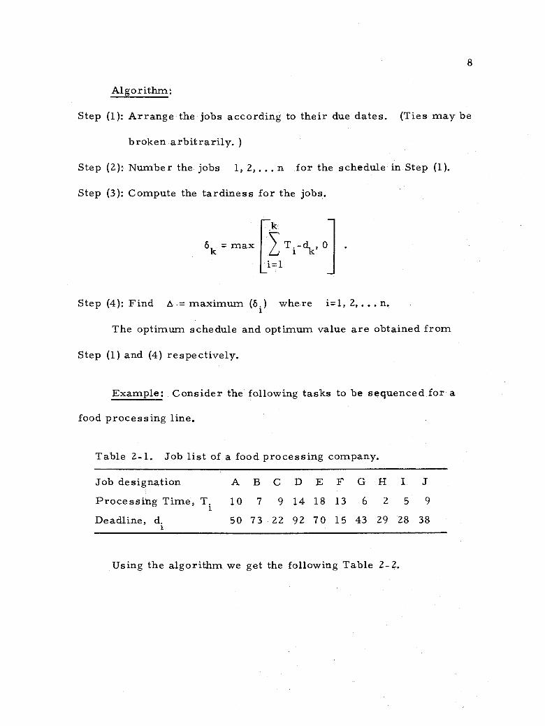
Algorithm:

Step (1): Arrange the jobs according to their due dates. (Ties may be

broken arbitrarily. )

Step (2): Number the jobs 1, 2, ... n for the schedule in Step (1).

Step (3): Compute the tardiness for the jobs.

6k = max Ti-d., 0

i=1

Step (4): Find A. maximum (6.) where i =1, 2, ... n.

The optimum schedule and optimum value are obtained from

Step (1) and (4) respectively.

Example: Consider the following tasks to be sequenced for a

food processing line.

Table 2 -1. Job list of a food processing company.

Job designation A B C D E F G H I J

Processing Time, T. 10 7 9 14 18 13 6 2 5 9

Deadline, d. 50 73 22 92 70 15 43 29 28 38

Using the algorithm we get the following Table 2 -2.

=

-k . .

Table 2-2. Computational method.

Job designation . A B C D E F G H - I J

Processing time, Ti 10 7 9 14 18 13 6 2 5 9

Deadline, d. 50 73 22 92 70 15 43 29 28 38

Optimum order, i 7 9 2 10 8 1 6 4 3 5

Finishing time 54 79 22 93 72 13 44 29 27 38

Lateness, 6. 4 6 0 1 2 0 1 0 0 0

The optimum sequence is F- C- I- H- J- G- A- E- B- D.and. the optimum

value is 6 (for job B).

Proof: Let

sequence S = 1, 2, 3,... (i -1), i, (i +1), (i +2), .. , n,

and

sequence 5' = 1, 2, 3, ... (i -1), (i +1), i, (1 +2), , n.

where 1, 2, 3, ... n are the job numbers.

Thus

and

= di' "

Ti Ti+1

for j i or (i +1)

9

T, _ J

dj

_

= T! T. Ti

di di+l

d = d' i+1 di

-

J

}

i+l

=

10

Also,

if

ój =S for j

A<Ad

max (6. Ô.

i+1

max Tj-di, /T.-d. d+1 j=1 j=1

or i+1.

< max (ói'öi i+1)

< max

`1 i+l

Tj di' Tj-di+l j+1 j=1

Replacing the T1 their equal T, 1

values we have: 1

i

max

j=1

T.-d., J 1

i+1

Tj-di+1

j=1

1+1

< max

Subtracting from each side L T.

j =1

or

or

i-1 i+1

Tj+Ti+l di+1' Tj-di

j=1 j=1

max ( -Ti +1 di' -di +l) < max (- Ti di +1'

-d.)

-min (T, +d., d )' < min (T.+d. , d. ) 1+1 1 i+1 - 5 +1

min (Ti +di+1, +1' d.) < min (Ti

+1 +di' di +1)

Since all Ti are positive, if di < di +1 this condition is met.

by

/ /

J J

J

Therefore, if di < d. , then 1- 1+1

11

A < A'. It can be stated that

the maximum tardiness can be minimized if the jobs are arranged ac-

cording to their due dates.

Hence, it is obvious that whenever it is possible to complete all

the jobs by their due dates, this can always be done by ordering them

according to due date.

B. Completion Times

The completion time for j_th job, if the tasks are processed

in a numerical order (job 1 first, job 2, second, etc. ), is j

Ti, where Ti is the processing time for the i -th job. The 1 1

i =1 sum of completion times for all jobs is

The waiting time for j -th job, j -1

the same numerical order, is n j -1

oder all jobs is T.,

j=1 i=1

n

i=1

Ti. j =1 i =1

if the jobs are processed in

Ti and the sum of waiting times

n

Ti + Ti

i=1 j=1 i=1 i=1

where T. is a constant. Hence, minimizing the sum of comple- t

i =1 tion times is the same as minimizing the sum of waiting times.

n j

n

n j j-1

Ti /

/

L

12

1. Sum of Completion Times

Case (a) Criterion: minimize the sum of completion times.

Smith (1956) has developed a method which enables one to obtain the

optimal schedule.

Computational Method:

Step (1): Arrange the jobs in the non -decreasing order of their proces-

sing times.

Step (2): Number the jobs of the sequence in Step (1).

Step (3): Calculate the completion times (C.) for the jobs, the opti-

mal sum of completion time (Z) and the optimal sum of

waiting time (W),

C.= T. J

i=1

n

i

W - Z - T.

i=1

The sequence in Step (1) gives the optimum schedule, where the

objective is to minimize the sum of completion times. This is also

the optimum schedule where the sum of waiting times is minimized.

Z =

j=1

C. J

/

J

13

Example: Consider the following jobs which are to be scheduled

in a boring mill (a single stage processing facility):

Table 2 -3, Job list for a boring mill.


Processing time, Ti 9 35 12 18 56 49 13 18 17 23

From the algorithm, we obtain the Table 2 -4.


Job designation AB C D E F G H I J

Processing time, T. 9 35 12 18 56 49 13 18 17 23

Optimum order 1 8 2 6 10 9 3 5 4 7

C. 9 145 21 87 250 194 34 69 51 110 i

Z = 970

W = 970 - 250 = 720.

The optimum schedule is A- C- G- I- H- D- J- B -F -E. The sum of corn-

pletion times is 970 and the sum of waiting times is 72Ó.

Proof:

i=1

n

Ci = L / T. = L(n+l-j)Tj i=1 j=1 j=1

The sum is the least only if T1 < T < T3...< Tri

i n n

14

Case (b) Criterion: minimize the sum of completion times.

Restriction: Each job must be completed by its due date.

In (1956), Smith described an algorithm for this problem based on

the method for minimizing the maximum tardiness (Chapter II, A) and

also on the method for minimizing the sum of completion times

(Chapter II, B).

The algorithm can be stated as follows:

Step (1): Arrange the jobs according to their due dates. Compute the

completing time for the jobs. If all jobs can be completed

by their respective due dates, the following steps can be fol-

lowed and an optimal schedule can be obtained. If not, the

problem is infeasible.

Step (2): If the k -th job (which is not the last job in the schedule we

got in Step 1), has the properties

n

i=1

Ti

n

and (ii) Tk > Ti for all i for which d. > Ti then the

i =1

k -th job is sequenced last. (The order of the remain-

ing (n -1) jobs is not disturbed. )

Step (3): Now, we have (n -1) jobs to be scheduled in the first (n -1)

order- positions. By "the job j scheduled in an order -

position p, " we mean that prior to this job being placed on

(i) dk >

/

15

the facility for processing, (p -1) jobs have previously been

processed through. Among the remaining (n -1) jobs, a

job is chosen having the properties (i) and (ii) stated in Step

(2) and scheduled in order -position (n -1). The same pro-

cedure is repeated and the order -positions (n- 2),(n- 3),...,2,1

are determined.

The complete order of the jobs is the optimum schedule and the

sum of completion times of this schedule gives the optimum. value.

Example: The planning section of a steel mill has seven orders

whose due dates and processing times (setup times are included) are

known. These tasks are to be sequenced so that the sum of comple-

tion times is to be minimized and they are completed by their due

dates. The tasks are to be scheduled on an automated production line.

Table 2-5. Job list of a steel mill.

Job designation A B C D E F G

Processing time, Ti 2 3 4 3 8 5 12

Deadline, days, di 25 43 8 12 38 29 19

The jobs are first arranged according to their due dates, to see

if the problem is feasible.

i

Table 2 -6. Schedule according to due dates.

Job designation C D G A F E B

Processing time, days, Ti 4 3 12 2 5 8 3

Deadline, days, di 8 12 19 25 29 38 43

Completing time, days, Ci i 4 7 19 21 26 34 37

For all jobs, C. < d, and the problem is feasible.

We note in Table 2 -6 that job E has the properties

and

dE > / Ti (i. e. , 38 > 37)

i=1

TE >-TB (i.e., 8> 3)

16

Hence, job E is schedules in order -position 7. The revised schedule

is shown in Table 2 -7.

Table 2 -7. Improved schedule No. 1.

Job

Ti

d. i C. i

CD 4

8

4

3

12

7

G

12

19

19

A

2

25

21

F

5

29

26

BE 3

43

29

8

38

.37

Now, the first six jobs, namely C, D, G, A, F and B are to be

scheduled in the first six order -positions. Job F has the properties

with respect to its deadline dF, and processing time as stated TF

..

17

in the algorithm. Therefore it is scheduled in the order position

The revised schedule is shown in Table 2-8.

Table 2-8. Improved schedule No. 2.

Job

T. i d. i C. i

CD 4

8

4

3

12

7

GA 12

19

19

2

25

21

BF 3

45

24

5

29

29

8

38

37

Continuing the same procedure, we determine the optimum

schedule.

Table 2-9. Optimum schedule.

Job

T. I.

d. i

C . i

D

3

12

3

C

4

8

7

G

12

19

19

A

2

25

21

BF 3

45

24

5

29

29

E

8

38

37

The optimum schedule is D- C- G- A -B -F -E and the optimum

value is 140.

Proof: Let S be the ordering 1, 2, 3, ... ,n and let it be so

chosen that with the tasks in this order all jobs can be completed by

their due dates. Let I n be the set of indices for which

di > L Ti.

i=1

6.

E

i i

Since the ordering S is such that all jobs are completed by

their due dates, we have that is in the set Ixl

18

Suppose that k is the index of the object with the largest val-

ue of T. for i in the set In. (If this is not unique, we choose i

one arbitrarily from those which are the largest. )

Now let S' be the ordering obtained from S by interchang-

ing the k -th and n -th terms.

So,

and

Now for

d. =d!

_ r

Tk n

Tn _ t k

__ t dk n

d =dkn n '

j<k, C'=

for i k or n.

TI

i=1 i=1

Since Tk > Tn and for k< j < n,

C! = LTi= L Ti+Tn - Tk=Cj+Tn - Tk<

i=1 i=1

n

1 L

n

n

L T1 CJ

n

Ti = Ti :'

_

J J

19

n n

Cñ=LTi=LTi=Cn. i=1 i=1

Therefore, taking the sums of C's,

n n

C! < C.1 . 1 - i

i=1 i=1

Also, all jobs are completed by their respective due dates under the

new ordering S', since for i k or n we have

and

C! < C. < d. = d! 1 - 1- 1 1

C. '< n T. d

= dk i=1

n

C' n

i=1

T.<d.k=d'. 1- n

In this. case, S is a schedule in which all jobs are completed by

their respective due dates and we have found an ordering S' with

the k -th job last, which minimizes the optimizer. The k -th job

has the properties n

(i) dk > Ti and

i =1 (ii) Tk > Ti for all i for which di

n

i=1

T.. 1

i

)

#

>

Hence, the theorem can be stated ásß:

If all jobs, 1, 2, 3,... , n, can be completed by their due

dates, then there is an ordering of the jobs with the k -th job last n

which minimizes Ci9 subject to completion of all jobs by their

20

i =1 respective due dates if, and only if, the k -th job has the above two

p rope rtie s.

If the jobs are arranged in the monotonically increasing order

d., and this order is such that i

J

dj-1 < Ti < d

1=1

for all j (taking do = 0),

then we cannot find a job among these j -jobs having the properties (i)

and (ii) given in the algorithm. Hence, this schedule is the only ar-

rangement by which all jobs can be completed on time and is there-

fore the optimum schedule.

We arrange the jobs according to their due dates in the initial

feasible solution. In each of the consecutive steps, we rearrange the

jobs in the non -decreasing order of T., as far as admissible, and

also we see that the jobs are completed by their respective due dates.

Hence, if the jobs are arranged in a non- decreasing order of T.

and still meet their due dates, then one cannot decrease the value of

the optimizer by rearrangement, that is, the value of the optimizer

of

/

x--.J o

i

21

for this order is the lower bound (the least possible value) on its

values.

2. Weighted Sum of Completion Times

Priority of a Job: The priority or importance of jobs are taken

into account in sequencing by assigning a weighted index to each job.

Let (a.(> 0) be the weighted index for job i.

The bigger the ai value, greater the job importance is; and

smaller the a. value, lesser the job importance is.

The weighted completion time of a job i is a.C., where

Ci is the processing time for job i.

Case (a): Criterion: Minimize the weighted sum of completion

times.

Smith (1956) presented a method to determine the schedule that n

would minimize the weighted sum of completion times, n

Theorem 2 -1: The sum

a.0 .. J J

j=1

a.C. is minimized over all order - J J

j =1 ings of the n jobs if the jobs are arranged so that (Ti /ai) /a,) form

a non -decreasing sequence.

Proof: Let S be the sequence 1, 2, 3, ... ,n and let S'

be the same schedule except with i and i +l interchanged.

So, sequence S' = 1, 2, 3, ... (i-1), i +l, i, (i +2)... n. Thus

LLJJ

and

Thus

or

C. =Cp 3 3

for or i+1

for j or i +l.

Now schedule S is as good as or better than S' if

a. 1

n

a.C. j

j=1

n

a.C. + a. C. < a i ° ° C! 1 1 1+1 1+1

Ci ° + a i+1 i+1

Subtracting

from both sides

+ ai+1

a. 1

i+1

j=1

ai+1

T.+T. + ai+1 J 1+1

j=1

+ a.

22

=T Ti "'

J

aj = a I

T. = Ti+1 1 i+1

j i

T.

j=1

i

L T.

j=1

i-1

Ti+1 _ Ti

ai aì+1

a. . = a.'

< a!G' - J

j=1

i-1

J j=1

L

Ti+1

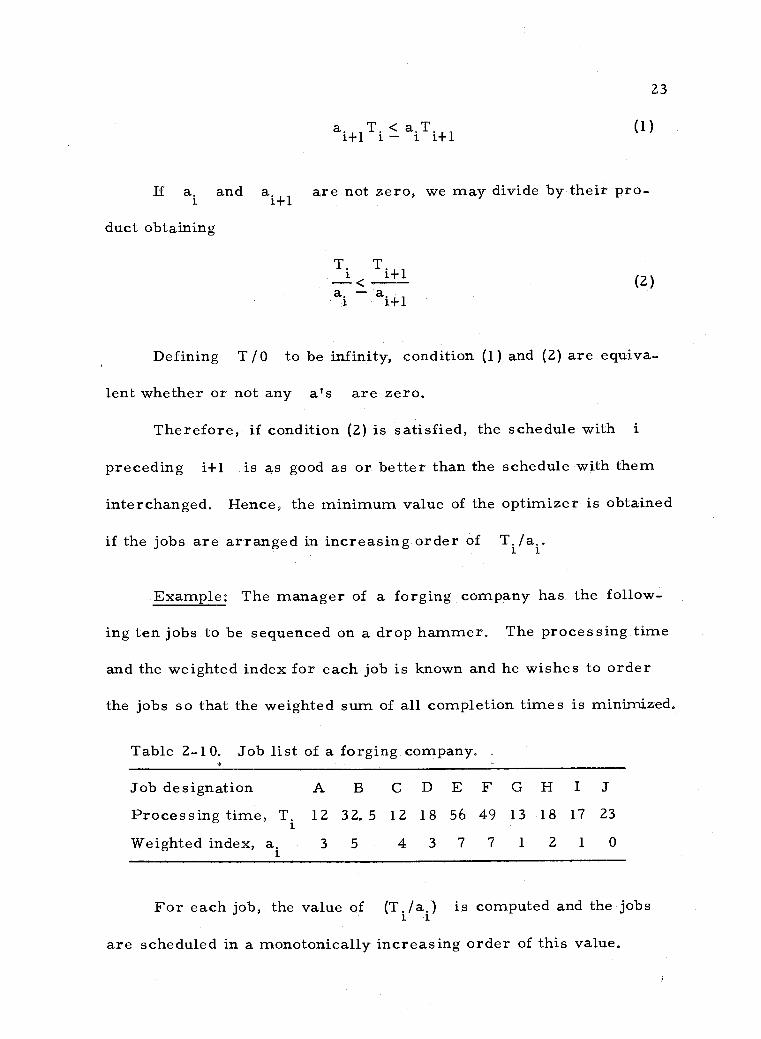
ai+1Ti - < aiTi+1

23

(1)

If ai and ai +1

are not zero, we may divide by their pro-

duct obtaining

Ti Ti+1 -<

ai - ai+l (2)

Defining T /0 to be infinity, condition (1) and (2) are equiva-

lent whether or not any a's are zero.

Therefore, if condition (2) is satisfied, the schedule with i

preceding i +l is as good as or better than the schedule with them

interchanged. Hence, the minimum value of the optimizer is obtained

if the jobs are arranged in increasing order of T./a..

Example: The manager of a forging company has the follow-

ing ten jobs to be sequenced on a drop hammer. The processing time

and the weighted index for each job is known and he wishes to order

the jobs so that the weighted sum of all completion times is minimized.

Table 2 -10. Job list of a forging company.

Job designation

Processing time,

Weighted index, ai

T.

A

12

3

B

32.5

5

C

12 18

4

D

3

E

56

7

F

49

7

G

13

1

H

18

2

I

17 23

1

J

0

For each job, the value of (T./a.) is computed and the jobs

are scheduled in a monotonically increasing order of this value.

24

Table 2.-11. Computation method.

Jobs

T. i

a. i T. /a.

i i Optimum

order Ci

a.C.

A

12

3

4

2

24

72

B

32.5

5

6.5

4

74.5

372.5

C

12

4

3

1

12

48

D

18

3

6

3

42

126

E

56

7

8

6

189.5

1326.5

F

49

7

7

5

133.5

934.5

G

13

1

13

8

220.5

220.5

H

18

2

9

7

207.5

415

I

17

1

17

9

237.5

237.5

J

23

0

00

10

260.5

0 i i

value

The optimum order is C- A- D- B- F- E- H -G -I -J and the optimum n

i=1

C. is 3752. 5. i

Case (b): Criterion: Minimize the weighted sum of completion

times.

Restriction: Each job must be completed by its dead-

line.

This is similar to the case described in Chapter II,

Section 1(a).

Jobs are arranged according to their due dates. If all jobs are

completed by their respective dead line, the problem is feasible.

The k -th job is ordered last if it has the properties:

(i) dk > T.

i=1

i

- ..

25

and (ii)

for all i for which

Tk Ti -> - ak ai

n

i=1

In consecutive steps the order -positions, n,n- 1,n.2, ... , 2,1

are determined and this is the optimum schedule.

Example: The manager of a forging company has the following

jobs to be scheduled on a drop hammer. The processing time, the

weighted index and the dead line for each job is known. He wants to

determine the optimum schedule and the value of it, where the objec-

tive is to minimize the weighted sum of completion times subject to

the condition that each job is completed by its due date.

Table 2 -12. List of jobs for a drop hammer.


Processing time, T. 12 9 18 35 49 56 18 13 17 23

Weighted index, ai 4 3 3 5 7 8 2 1 1 1

Deadline, d. 100 89 252 100 251 215 104 32 31 205

We arrange the jobs according to due dates and find from Table

2 -13 that for each job C. < d.1 . Hence, the problem is feasible. 1 -

-

d. > i- T.. i L [)'

i

26

Table 2 -13. Schedule according to due dates.

Job

T. i

a.

d. i

Order-position

C. i

A

12

4

100

4

51

B

9

3

89

3

39

C

18

3

252

10

250

D

35

5

100

5

86

E

49

7

251

9

232

F

56

8

215

8

183

G

18

2

104

6

104

H

13

1

32

2

30

I

17

1

31

1

17

J

23

1

205

7

127

The jobs are sequenced according to due dates in Table 2 -14

and it is found that job E has the properties:

(i) dE> i=1

TE Ti _>_ aE-ai

T. as 7 > 6 i

as 251 > 250.

Job E is assigned to the order position 10 and this change is incorpo-

rated in Table 2-15.

Table 2 -.14. Improved schedule No. 1.

Job

T. i

T. /a. i i

d. i

C. i

I

17

17

31

17

H

13

13

32

30

B

9

3

89

39

A

12

3

100

51

D

35

7

100

86

G

18

9

104

104

J

23

23

205

127

F

56

7

215

183

EC 49

7

251

232

18

6

252

250 I

27

The same procedure is continued and we get the following sched-

ules as shown in Tables 2.-16 to 2 -18.


Job I H B A D G J F C E

T. i

17 13 9 12 35 18 23 56 18 49

Tia. i i

d. i

17

31

13

32

3

89

3

100

7

100

9

104

23

205

7

215

6

252

7

251

C. 17 30 39 51 86 104 127 183 201 250 i


Job I H B A D G J CF E

T. i 17 13 9 12 35 18 23 18 56 49

T. /a. i i

17 13 3 3 7 9 23 6 7 7

d. i 31 32 89 100 100 104 205 252 215 251

C. i

17 30 39 51 86 104 127 145 201 250

\ Table 2 -17. Improved schedule No. 4.

Job I H B A D G C F J E

T. 17 13 9 12 35 18 18 56 23 49

T. /a. i 1

d. i

17

31

13

32

3

89

3

100

7

100

9

104

6

252

7

215

23

205

7

251

C. 17 30 39 51 86 104 122 178 201 250 i

l

i

J

28

Table 2 -18. Optimum schedule.

Job

T. i

T./a. i i

d. L

C. i

a. i

a.C.

H

13

13

32

13

1

13

I

17

17

31

30

1

30

B

9

3

89

39

3

117

A

12

3

100

51

4

204

D

35

7

100

86

5

430

GC 18

9

104

104

2

208

18

6

252

122

3

366

F

56

7

215

178

8

1424

J

23

23

205

201

1

201

E

49

7

251

250

7

1750 i i

The optimum schedule is H- I- B- A- D- G- C -F -J -E and the opti-

mum value [ a. C 1 i

is 4,743.

C. Penalty Cost

The consumer and the supplier enter into a business contract

for the supply of one or more products or for executing a particular

task. The project is expected to be completed on or before a definite

date, known as a deadline or due date. Normally conditions are also

stipulated for situations when the goods are not delivered by the dead-

line. There may, for example, be a reduction in payment (by the

consumer to the producer) of a certain fixed amount for every day

which the task goes uncompleted beyond the deadline.

The amount of penalty imposed on the producer can be expressed

or approximated as a function of penalty coefficient and time. This

penalty or loss function may be classified either as linear or non-

linear.

29

If the jobs are not completed by the due date, then a penalty is

determined from this loss function.

1. Linear Loss Function

Let us suppose that a task, i, imposes a penalty of

max (0, p. (C. 1 1 1

-d. )), where

pi is the penalty coefficient for job i

C. is the completion time for job i

d. is the deadline for job i. i

In other words, there is no loss if the task is completed on or

before time d., but a loss of p units for every unit of time after

di during which the task is incomplete.

McNaughton (1959) has formulated a method for scheduling the

jobs with past deadlines in a single stage processor, so as to mini-

mize the total penalty cost.


Step (1): For each job, calculate r. pi t. 1

where p. is the penalty coefficient of job i,

t, is the processing time of job i. i

Step (2): Arrange the jobs according to the decreasing values of r.

(ties, if any, are broken arbitrarily). The optimum sched-

ule is the one obtained in Step (2).

30

Example: A printing press has the following jobs, whose dead-

lines have already passed. The management wishes to schedule the

tasks in the press (a single processor) so that the total penalty is

minimized.

Table 2 -19. Job list for a printing press.

Job, i A B C D E F G H

Processing time, t. 10 8 17 45 49 36 58 25

Penalty coefficient, pi 70 32 40. 8 58. 5 8.82 450 110 118. 8

i

P The value of r = 1 for each job is calculated and the jobs

t. i

are sequenced in a decreasing order of r.. This is shown in Table

2 -20.


Job, i A B C D E F G H

Processing time, t. 10 18 17 45 49 36 58 25

Penalty coefficient, pi 70 32 40.8 58. <5 8.82 450 110 118.8

pi /ti 7 4 2.4 1.3 0.18 12.5 1.9 4.75

Order of processing 2 4 5 7 8 1 6 3

The optimum schedule is F- A- H- B- C- G -D -E.

Proof: Let C be the joint loss on (i) and (j), computed

cumulatively up to time t. Then the loss on (i) and (j), if (i)

i

31

precedes (j), is

C + tipi + (ti +t J

)p .

J

The loss, if (j) precedes (i), is

C + (tipi) ) + (ti+tj )pi

Taking C' = C + t.p. + t.p., the two losses are, respectively, I I J J

C' + t.p, and C' + t.p.. If r. (=p./t.) > r.(=p./t.) then I J J 1 1 1 1 J J J

tipi > tipi and the first loss is less than the second; then, the loss is

less if (i) is done before (j). Hence, the jobs are to be scheduled

such that r.'s of the jobs are in a non -ascending order to minimize

the cumulative penalty cost.

Schild and Fredman (1961) have developed an algorithm to de-

termine the optimum schedule in a single stage processor when the

linear loss function and the processing time for each job are known.

Algorithm:

Step (1): Arrange the tasks according to deadlines, d.I . If in this

arrangement all tasks are finished before their deadlines

then the total loss is zero and this schedule is optimal (Con-

dition A).

Step (2): If Condition A is not satisfied, arrange the tasks in the order

of non -increasing r.(=p./t.). If in this arrangement every 1 1 1

t

t J

32

task is completed after its deadline, then this schedule is

the optimal (Condition B). If not, go to Step (3).

Step (3): Take the schedule (arranged in a non -increasing order of

r.) of Step (2). Number the jobs in the serial order as

1, 2, 3...n. Check the jobs in the order 1, 2, 3, ... and

find which of them is completed before its deadline. Let it

be job 'i'. Taking job i +l as j and job i as 1,

substitute the parameters in the Criterion C.

where

Criterion C:

d'-t. I

+ (d.'-t.) 1(dl'-t)ôj + pltj(1-ój) - pj J J J J

j_1

> (pit.-p.ti) as j=2, 3, 4. . .

i=1

[ lt_d'+t I+(t.-d'+t )] ó.

i 1 J 1 1

J [21t.-d 1+t I

1

]

óJ . =0 J

if t.<d'-t 1 1

ó j= 1 if tj > d -

ój=1 if tj=d1'-tl

and the deadlines d. 's are calculated taking the starting time of job

i as zero. If for (i +l) the criterion is satisfied, move (i +1) in

I

J

J

J J 1

L

33

front of (i). If for (i +1) the criterion is not satisfied, then try

for (i +.2), (i f3), ... etc.

For tasks that are completed by their deadline, Step (3) is re-

peated till either all tasks finish after their deadline, or all tasks ex-

cept for a group of tasks at the end of the schedule finish after their

deadlines.

The final sequence is the optimum order and the cumulative

penalty cost for this schedule in the optimum value.

Example: The following jobs are to be scheduled in a batch

processing computer system with a single central processing unit so

that the total penalty cost, if any, is minimized.

Table 2 -21. Job list. i t. (days) . d. (dates) pi (dollars)

A 10 39 70 B 8 50 32 C 17 135 40.8 D 45 255 58.5 E 49 250 8.82 F 36 30 450 G 58 120 110 H 25 75 118.8

Step (1): To see if all jobs can be completed by their deadlines, we

arrange the jobs according to their deadlines and compare

the completion time C. with deadline d. of each job. 1 1

In Table 2 -22 column 6 shows that there are some jobs which.

34

are not completed by due dates. Hence, condition A is not

satisfied.

Step (2): To see if the condition B is satisfied, we arrange the jobs in

the monotonically decreasing order of r. ( =p, /t.) and check

if all jobs are completed after their respective due dates.

In Table 2 -22, column 9 shows that there are some jobs

which are completed by their respective due dates. Hence,

condition B is not satisfied.

Step (3): Next, we take the schedule in which the jobs are arranged in

a non- increasing order of r. (Table 2 -22, column 8). We

find from Figure 2 -1 that job H is completed before comple-

tion time. We interchange the values of job H (i) and of

job B (i +l) in Criterion C.

F C G D E

o

M/A0V.Z \V":///iAN \ 36 46 71 79 96 154 199

Figure 2 -1. Gantt chart for a feasible schedule.

248

A

1

1

1

H

i

Table 2 -22. Computational method.

1 2 3 4 5 6 7 8 9 10 11 12 13 Step 3

Given data Step 1 Step 2 Schedule Schedule Schedule Schedule Schedule 3 -C

Jobs t i

d. i p. i 1

C. i

r.; i 2

C. i 3-A 3 -B optimal C.

i

A 10 39 70 2 46* 7 2 46 2 2 2 46

B 8 50 32 3 54* 4 4 79 3 3 3 54

C 17 135 40.8 6 154* 2.4 5 96* 5* 6 6 154

D 45 255 58.5 8 248 1.3 7 199* 7* 7* 7 199

E 49 250 8.82 7 203 .18 8 248* 8* 8* 8 248

F 36 30 450 1 36* 12.5 1 36 1 1 1 36

G 58 120 110 5 137* 1.9 6 154 6 5 5 137

H 25 75 118.8 4 79* 4.75 3 71* 4 4 4 79

Penalty 7, 858 7, 533 6, 438 6, 438

* Denotes the job which does not satisfy the condition A and /or B.

Hence,

And

t. = 8 J

36

- t1 = [ (dl-cA)-t l] = [ (75-46)-25] = 4

tj > (dl'-t1).

ö. = 1 ... case (2).

pl = 118. 8,

dlt - t 1

= 4

p. = 32

d'-t.=4 J J

Substituting these values in Criterion C,

(118. 8)(4) - (32)(4) > (118. 8)(8) - (32)(25)

347 > 150

Criterion C is satisfied and job B is scheduled before H. Thus

we obtain schedule 3 -A (Table 2 -22, column 10). Following the same

procedure, we get the schedules 3 -B and 3 -C as shown in Table 2 -22,

columns 11 and.12.

The optimum schedule is F- A- B- H- G -C -D -E and the minimum

total penalty is 6, 438 dollars.

Schild and Fredman (1961) have presented a proof showing that

dl'

37

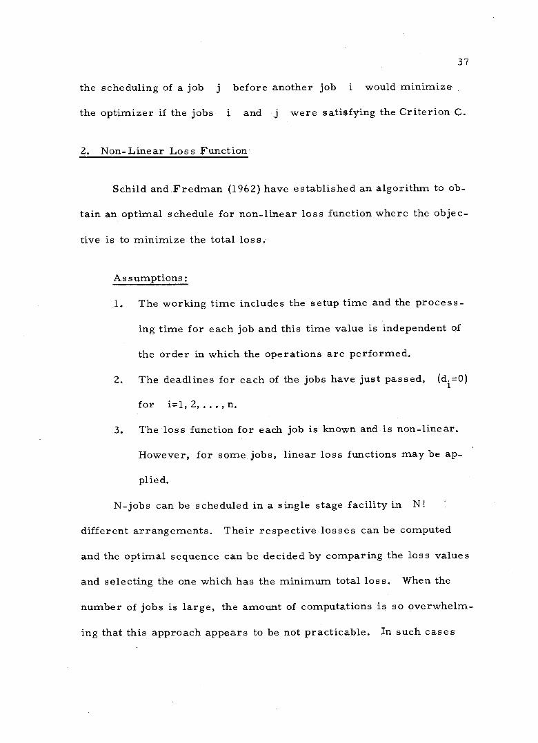
the scheduling of a job j before another job i would minimize

the optimizer if the jobs i and j were satisfying the Criterion C.

2. Non- Linear Loss Function

Schild and Fredman (1962) have established an algorithm to ob-

tain an optimal schedule for non -linear loss function where the objec-

tive is to minimize the total loss.

Assumptions:

1. The working time includes the setup time and the process-

ing time for each job and this time value is independent of

the order in which the operations are performed.

2. The deadlines for each of the jobs have just passed, (di =0)

for 1 2 , , n

3. The loss function for each job is known and is non -linear.

However, for some jobs, linear loss functions may be ap-

plied.

N -jobs can be scheduled in a single stage facility in N!

different arrangements. Their respective losses can be computed

and the optimal sequence can be decided by comparing the loss values

and selecting the one which has the minimum total loss. When the

number of jobs is large, the amount of computations is so overwhelm-

ing that this approach appears to be not practicable. In such cases

1

i

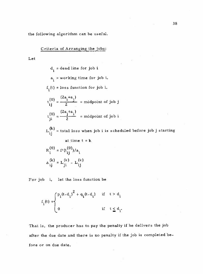
the following algorithm can be useful.

Let

Criteria of Arranging the jobs:

d. = dead line for job i

a. = working time for job i.

fi( t) = loss function for job i.

(tai +a.)

iJ _

2

- (2aj+ai)

J1 2

= midpoint of job j

= midpoint of job i

38

Lk) = total loss when job i is scheduled before job j starting 1J

at time t = k

Rio) = f t (ti °))tai

(k) = Lk) - Lk)

1J 31 13

For job i, let the loss function be

pi(t -di)2 + qi(t -di) if t > di

if t < d.. 1

fi(t) =

That is, the producer has to pay the penalty if he delivers the job

after the due date and there is no penalty if the job is completed be-

fore or on due date.

(0)

-

a

(0)

0

39

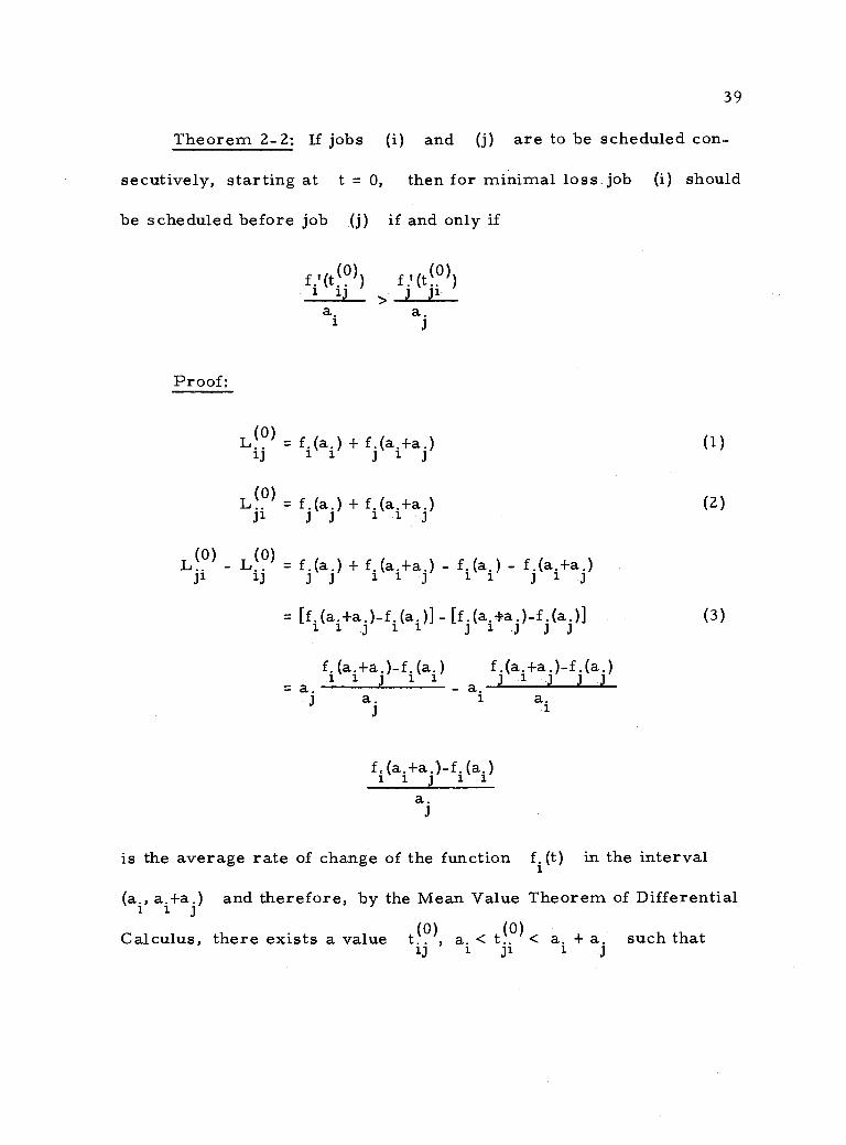
Theorem 2 -2: If jobs (i) and (j) are to be scheduled con-

secutively, starting at t = 0, then for minimal loss, job

be scheduled before job (j) if and only if

Proof:

fi`(tl)) fJ'(t)) >

a. a. 1

J

L) = f.(a.) + f.(a.+a.) 13 1 1 J 1 J

L0) = f.(a.) + f.(a.+a.) 31 J J i 1 J

L. - L0) = f.(a.) + f.(a.+a.) - f.(a.) - f.(a.+a.) Ji 1J J J 1 1 J 13. J 1 J

_ [f.(a.+a.)-f.(a.)]-[f.(a.+a.)-f.(a.)] 1

1 J 11 J 1 J J J

= a. J

f.(a.+a.)-f.(a.) 1 1 3 1 1

- a. a. 1 a. J 1

f.(a.+a.)-f.(a.) J 1 J 3 3

f,(a.+a.)-f.(a.) 1 1 J 1 1

a. J

(i) should

(3)

is the average rate of change of the function f. (t) 1

in the interval

(a., a. +a.) and therefore, by the Mean Value Theorem of Differential 1 1 J

Calculus, there exists a value t.. , a. < t.» < a. + a. such that 13 1 Jl 1 J

(1)

(2)

Hence,

fi(ai -fi(ai) aJ = f i (tiÓ))

3

fi(ai +aj) -fi(ai) 1 1 3 1 I.

a. J

0 2piti) + gi = pi(2ai+a.), + qi 3 J

- p. (2a.+a.) + q. 1 1 3

(0) (0) = 2pitiÓ, + qi

(2ai+a ) a. O J

J =

2 = ai + .

40

(4)

0 )

0 Similarly, it can be shown that there exists a t.. , a. < t.. < (a.+a.) 31 3 31 3 1

such that

f (a.+a.

a. 1

where

so, Equation (3) becomes,

-f(a

J Ji

ai+2a 31 2

L(0) - L(0) = a.f.'(t)) - a.f!(t(0)).

31 i3 .3 1 13 1 3 31

L(0) < L) if and only if 13 31

fi (t1)) f! (t)) a. a.

1 3

(7)

(8)

(9)

1 1 1 1

(5)

(6)

) 1 J J J=

1

i iJ

t(0)

>

that is,

R. > R. 1 J

Graphically, the positions of t) and t) can be shown as iJ Ji

The schedule is determined by the value of f qt) at a single

point only, and it is not dependent on f(t) explicitly at all.

Theorem 2 -3: If d. = d. = 0 and (i) and (j)

uled in (a. +a.) consecutive units of time starting at t = k, then J

are ached-

(i) should be scheduled-before (j) if and only if R:k) > Rk). J

Case (2): Starting at t = k, k > O.

L) = f. (k+a. ) + f.(k+a.+a.) 1J 1 1 J 1 J

Lk) = f.(k+a.) + f.(k+a.+a.) J1 J J 1 1 J

In a similar way, as in (1) and (2), it can be shown that

41

(10)

ai

a )

a .1 2

a

-14(2)-

i J

1

where

and

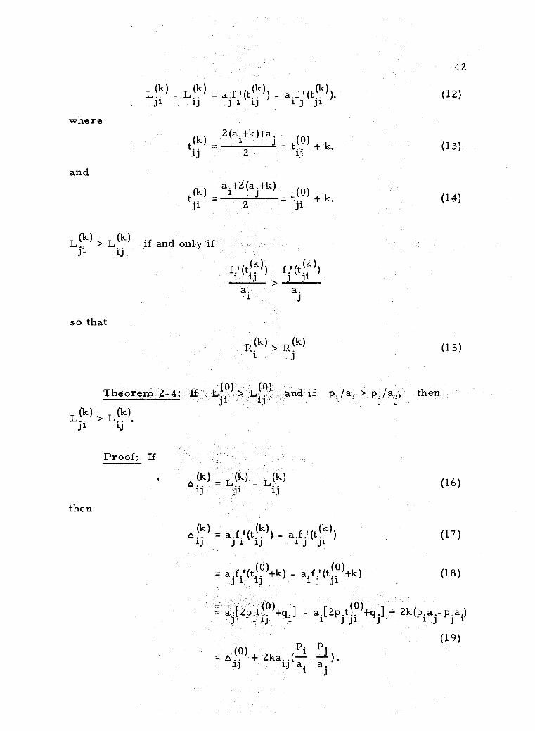
L(k) - L) (t1J )) aif'(tk)).

t(k) 2(a.+k)+a. (0) - t.. + k.

1J 2 1J

a +2(a.+k) t(k) i .J = t(°) + k. Ji 2 ji

L> L(k) (k) if and only if J1 iJ

so that

Theorem 2 -4: If

Lk) > Lk). J i 1J

Proof: If

then

fi (ti )) f'(tjk)) > a. a.

1 J

R. > R. 1 J

)

42

(12)

(13)

(14)

and if pi /ai > pia., then

0 (k) L(k) L(k) = Jì lj

oi ) = afi'(ti (k) (k) - aif'(tk))

= ajfi (ti)+k) - aif'(t)+k)

0 0 = a;[2piti +qi] - ai[2pJti +q] + 2k(pia-pai)

J

(19)

(15)

(16)

(17)

(18)

pi P. = o) + 2ká....(---)

13 13 a. a.

= aJfi -

-

> L J1 1J 11

-

j1 ij

L(k)

. Lei

43

It can also be stated as: If for the minimal loss (i),, is to be

scheduled before (j) when starting at t = 0, (i) and (j) being

scheduled consecutively, then (i) should be scheduled before (j)

also when starting at t = k, if p. /a. > p. /a.J . It is to be noted, 1 1 J J

that this is a sufficient condition. Actually, if p. /a. < p.3 /a.3 , (i)

would still be scheduled before (j) when starting at t = k, pro-

vided ) 2k< 13

(pjai-pia.)

Theorem 2 -5: If d. = d. = 0 and one of the jobs (i or j) 1 J

is started at t = 0, and k units of time after its completion the

other job is started, then (i) should be scheduled before (j) if

and only if

fi1(ti(k)j) fj (tjtj(k)i) a.+k a.+k

Li(k)j fi(ai) + fj(a. +aj +k)

1 (21)

L. J(k)i J

= fi(ai) i 1 J + f (a. +a. +k) (22)

Proceding in a similar way as with Theorem 2 -2, we have:

Lj(k)i - Li(k)J (a. +k)f it(ti(k)j) - (ai +k)fj'(tj(k)i) (23)

where

1 1 J

>

1 J

-

=

and

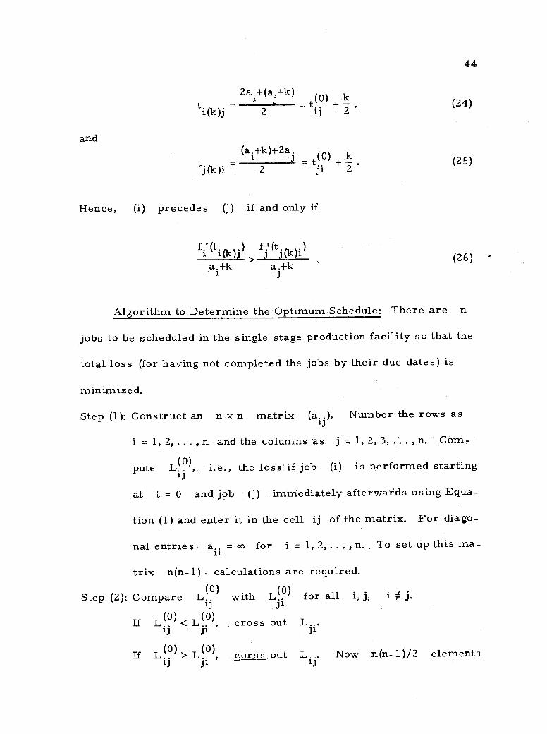
2a.+(aj+k) (0) k ti(.k)j = = ti + 2

(ai+k)+2aj (0) k tj (k )i 2 tji + 2

Hence, (i) precedes (j) if and only if

fie(ti fj (tj(k)i) )J) ) (k)i

a.+k a.+k

44

(24)

(25)

(26)

Algorithm to Determine the Optimum Schedule: There are n

jobs to be scheduled in the single stage production facility so that the

total loss (for having not completed the jobs by their due dates) is

minimized.

Step (1): Construct an n x n matrix (a..). Number the rows as

i = 1, 2, ... , n and the columns as j = 1, 2, 3,.... , n. Com-

pute L.. i.e., the loss if job (i) is performed starting ij

t = 0 and job (j) immediately afterwards using Equa-

tion (1) and enter it in the cell ij of the matrix. For diago-

nal entries a.. oo for i = 1, 2, ... , n. To set up this ma- n

trix n(n -1) calculations are required.

Step (2): Compare L ?) with L..) for all i, j, i j. iJ J1

If L. < L. , cross out L... iJ Jl J1

If L.0

> LJ), corss out L... Now n(n -1)/2 elements

i 2

1

at

=

#

J

"

)i

45

are available. Ties, if any, may be broken arbitrarily.

Step (3): Construct an n(n -1)/2 by n matrix where the rows are

the available n(n- 1)/2 elements in the first matrix. The

columns are numbered as k = 1, 2, ... , n° Now the entries

will be Li k where the first two subscripts refer to those J

jobs which survived the elimination process from the first

matrix, and k = 1, 2, 3, ... , n. For any particular row in

the matrix, that is, for any fixed i and j there will be

two entries which are undefined. For these two entries

L(0) = oo where k = i, j. The total number of calculations ijk

required for Li would be n(n- 1)(n -2/2. There will be J

only three entries with the same subscripts, namely, L.

L(k0) and (ki for any choice of tasks (i), (j) and (k).

J J

From these three entries, pick up the smallest one, say

L jki, and cross out the others. Now, in the second matrix

out of n(n- 1)(n -2)/2 entries only one -third will remain,

that is n(n- 1)(n -2)/3!

Step (4): In a similar way, construct an n(n- 1)(n -2)/3! by n

matrix whose entries will be L(0) etc. J

Continue the method and the n -th matrix will be an

n (n- 1(n- 2 )... 2 1 /n! by n matrix, that is, a 1 by n

matrix. Select the smallest entry. This is the minimum

loss and the order of the jobs is the required optimal schedule.

J

46

We note that when we go from one matrix to the next, the en-

tries of the previous matrix are used and only one additional calcula-

tion is required for each new entry. For instance

L Jk

= L(0)+ (loss due to task (k) starting (ai +a.) units after t = 0).

The following example is worked out by means of the algorithm devel-

oped above.

Example: The due dates for the following five jobs have just

passed and each of them require processing only in the milling ma-

chine. You are to recommend a schedule to the machine shop foreman

for these jobs so that the total loss (due to the penalty for not meeting

the due dates) is minimized. The durations, a2, and loss functions

are given below:

f1(t) = 2t al 1

= 2 days

f2(t) (t -1)3 a2 = 3 days

f3(t) = t(t2- 1) a3 = 3 days

f4(t) = . 5(t3+2) a4 = 2 days

f5(t)=t+2 a5=4days.

=

47

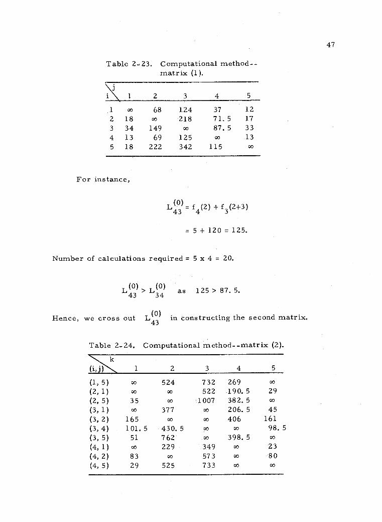
Table 2 -23. Computational method- - matrix (1).

J

i 1 2 3 4 5

1 00 68 124 37 12 2 18 co 218 71.5 17 3 34 149 o0 87.5 33 4 13 69 125 o0 13 5 18 222 342 115 co

For instance,

L4) = f4(2) + f3(2+3)

= 5 +120 =125.

Number of calculations required = 5 x 4 = 20.

L4)> L3 as 125 > 87. 5.

Hence, we cross out in constructing the second matrix.

Table 2-24. Computational method--matrix (2).

(i,j) k

1 2 3 4 5

(1, 5) o0 524 732 269 00

(2, 1) o0 0o 522 1900 5 29 (2, 5) 35 00 1007 382. 5 co

(3, 1) o0 377 00 206. 5 45 (3, 2) 165 co 00 406 161 (3, 4) 101. 5 430. 5 00 00 98. 5

(3, 5) 51 762 00 398. 5 0o

(4, 1) 00 229 349 co 23 (4, 2) 83 00 573 0o 80 (4, 5) 29 525 733 oo 00

L44)

For instance

48

L(0) L(0) + loss due to (2)

342 34

= 87. 5 + f2(8) = 430. 5

Number of calculations = n(n- 1)(n -2)/2 = 30

Table 2 -25. Computational method-matrix (3).

(i,j,k) 1 2 3 4

(2, 1, 5) co co 1745 695. 5 co

(3, 1, 5) o0 1376 o0 711. 5 co

(3, 2, 1) co o0 o0 666 179 (3, 2, 4) 426 co o0 o0 420 (3, 2, 5) 185 co o0 1026 oo

(3, 4, 1) co 830. 5 o0 o0 114. 5

(3, 4, 5) 120. 5 1429. 5 o0 co o0

(4, 1, 5) co 1023 1343 co o0

(4, 2, 1) o0 o0 1073 og 96 (4, 2, 5) 102 o0 1796 co co

Table 2 -26. Computational method-matrix (4).

m (19 9k,.Q ) 1 2 3 4 5

(3, 2, 1, 5) co co oó 1552 co

(3, 2, 4, 1) o0 oo co o0 442 (3, 2, 4, 5) 448 o0 o0 o0 o0

(3, 4, 1, 5) o0 2311. 5 o0 o0 0o

(4, 2, 1, 5) o0 o0 2820 oo o0

Table 2 ..27. Computational method- - matrix (5).

5

(3, 2, 4, 1, 5) o0 o0 o0 o0 442

5

n (i,j,k,.Q,m 1 2 3 4

=

The optimum schedule is 3- 2 -4 -1 -5 and imposes a penalty of

442.

49

Merits of the Algorithm: In the brute force method, n! cal-

culations are needed to compute all the feasible solutions. The opti-

mal schedule can be determined by comparison. The above algorithm

on the other hand, permits us to determine the optimum schedule in

N calculations, where

N = n(n-1) + n(n-1)(n-2)/2! + n(n-1)(n-2)(n-3)/3! + ...+ n

n(2n-1-

Table 2-28. Number of computations required for various number of jobs.

n N=n(2n-1-1) n!

3 9 6

4 28 24 5 75 120

10 51107 362880018 20 10 2. 4 x 10

We note in Table 2 -28 that although N is still relatively large

for large n, it is considerably less than n!.

D. Elapsed Time -- Scheduling on 'Not -Alike' Processors

When a manufacturer receives an order to produce a number of

items, normally he intends to complete the tasks as soon as possible

50

so that his processing facilities will be ready for further orders. The

number of processing facilities may be one or more of each type.

Processors are said to be alike if they can perform the same

operation with the same efficiency. Two processors are said to be

"not alike" if they perform the same operation with different efficien-

cies.

1. Three Jobs on Two Processors

McNaughton (1959) has presented decision rules for scheduling

three jobs on two processors which are not alike for different cases.

The criterion is to minimize the total elapsed time. Splitting the jobs

in processing is allowed in this method. By 'splitting a task in pro-

cessing' we mean that after a processor has started to work on a task

the operation can be interrupted for some time before the operation is

restarted again in the same processor or in another facility which

will perform an equivalent processing. For instance, it is possible

to split a job in two in a schedule, to do one part of it between time 2

and time 6 and the remaining part between time 9 and 14. A job may

be split in any number of parts and placed in as many equivalent pro-

cessors.

We shall consider a case, where three jobs (1), (2), and (3) are

to be scheduled on two not -alike processors, A and B.

51

Let

efficiency of A in processing job (i) ei efficiency of B in processing job (i)

Table 2 -29. Notations for processing times of 3 jobs on two machines.

Processors B

, t1

. t2

e3° t3


Step (1): Number the jobs so that

e > e2 > e

Step (2): In Table 2 -30, case 1, see if conditions (i) and (ii) are sat-

isfied. If they are satisfied, schedule job 1 in A and the

jobs 2 and 3 in B.

If case 1 is not satisfied, then check if case 2, conditions

(i) and (ii) hold good. If so, arrange job 1 in B and jobs

Z and 3 in A.

If case 2 is not satisfied, go to case 3 and so on. If

case 6 is not satisfied, go to Step (3).

Step (3): For cases 7-13, the conditions C, D and E (and others,

if any), are to be checked. In each case, if the job satisfied

all the conditions given as true and does not hold for those

A

tl t

t 2

3

el e2

52

given as false in Table 2 -31, choose that case, if not go to

the next case.

The schedule obtained is optimal and corresponding elapsed time is

the optimum value.

Table 2 -30. Decision rules for three jobs on two not -alike machines problem.

Case No.

Conditions Processors (i) (ii) for (1) for (2) for (3)

1 e1> 1 tl>e2t2+e3t3 A B B

2 e1 <1 eltl>t2+t3 B A A

3 e2 > 1 t2 > eltl + e3t3 B A B

4 e2 < 1 e2t2>tl+t3 A B A

5 e3 > 1 t3 > eltl + e2t2 B B A

6 e3<1 e3t3 3 3

> tl + t2 A A B

Example: Let us illustrate an example of scheduling 3 tasks on

2 not alike machines using the computational method:

t1 1

= 6 hours, el = 1. 3

t2 = 3 hours, e2 = 1. 2

t3 = 10 hours, e3 = 1. 1

The condition el > e2 > e3 is satisfied.

53

Table 2 -31. Decision rules for three jobs on two not -alike machines, problem.

Case No. C

7 true

Conditions E F

Processors

true true

Fvr(1) For{2) For(3)

A split B (2) in A: _

in (1+e2

)t2

A&B t1 +t2 -e3t3 (2) in B: = (1+e

2 )t

et+et3mt 2 2 1

8 false true true e3 > 1 A split split In A and B total time 't' equal. in in For (3), total time is 'V.

A &B A &B (try)

9 false true true (8) e3 > 1 split B split In A and B total time 't' equal.

false in in For (3), total time is 't'. A &B A &B

10 true false true (7) e 1

< 1 split split A In A and B total time 't' equal.

false in in For (1), total time is 'V. A &B A &B (try)

11 true false true (10 e3 < 1 split B split In A and B total time 't' equal.

false in in A &B A&B

For (1), total time is 't'.

12 true true false e > 1 2 -

13 true true false e2 < 1

split split in in A&B A&B

In A and B total time 't' equal. For (2), total time is 't'.

A split split In A and B total time 't' equal. in in For (2), total time is 't'. A &B A &B

Condition C: t1+t2 > e3t3

D: e2t2 + e3t3 > t

E: e2t2 < e2e3t3 +t 2 2 2 3 3 1.

D G

3

B

54

Case (1): Condition (ii) is not satisfied as t1 = 6 and

e2t2 + e3t3 = 14. 6

Case (2): Condition (i) is not satisfied as e 1

= 1. 3.

Case (3): Condition (ii) is not satisfied as t2 = 3 and

eltl 1

+ e3t3 3

= 18. 8.

Case (4): Condition (i) is not satisfied, since e2 = 1. 2.

Case (5): t3 = 10 and eltl + e2t2 = 11.4. Hence, condition (ii) is

not satisfied.

Case (6): e3 = 1.3. Hence, condition (i) is not satisfied.

Case (7): Condition C is not satisfied.

Case (8): Conditions are satisfied.

q fractional part of job (2) and p fractional part of job (3)

are to be processed in A as shown in Figure 2-2.

Processor A

Processor B

Job (3)

( (1-q)

Job(1) Job (2)

(1 -p)

Job (2) Job (3) Time = t

Figure 2 -2. Gantt chart for case (8).

The restrictions are satisfied for

p =e 3.3 and q = 10.1.

q

V// /i,

%//////////

Since this is not feasible, we go to the next case.

Case (9): Conditions are satisfied.

The jobs are to be scheduled as shown in Figure 2 -3, if it is

feasible.

Processor A

Processor B

Part p Part q

(1-q) /////_- Job (1) Job (2)

Figure 2 -3. Gantt chart for case (9).

(1 °P) \ \ \ \ \ \ \ \ \ \ \ \ \ \\

Job (3)

elapsed time = t

55

The computation yields p = 0. 68 and q = 0. 587 and hence,

the Gantt chart for the optimum schedule can be drawn as shown in

Figure 2 -4.

Processor A

Processor B

`\ \ \ 1 \ \ t \ \ \\\1\\\\\\\\ \ !//////////IJ .68 part of(3) 6.80

.587of(1)

.413of(1) 320

(2) i\\\\\\\\\\\\1V

6.80 .32 of (3)

Figure 2 -4. Gantt chart for optimum schedule.

10.32

10.32

Job (3) Job (1)

°'

v2r 4

'V% M%/////////%

56

The optimum value (total elapsed time) is 10.32 hours.

2. A Linear Programming Model

In the previous section (Chapter II. D -1) we have presented the

decision rules for determining the optimum schedule for 3 -job, 2-

machine problems. The facilities are "not- alike" and splitting jobs

is permissible. The criterion is to minimize the total make span.

In this section, we present our formulation of a model based on linear

programming for obtaining the optimal schedule for n jobs on m

single -stage processing facilities which are not -alike (that is, having

different efficiencies).

Let

Formulation of a Model:

t.. = time required to process job i in machine j completely. zJ

x.. = fraction (> 0) of job i processed in machine j. 1J -

t = time elapsed for processing the given set of jobs.

For example, if machine 4 requires 7 hours for processing job

3 completely and machine 4 has processed 3/21 of job 3, then this can

be represented as t34 = 7, x34 = 3/21 and x34 t34 = 1 hour. If

machine 6 requires 14 hours to process job 3 completely, then the

ratio of efficiencies of machine 4 to machine 6 with respect to job 3

is 2(= 14/7).

57

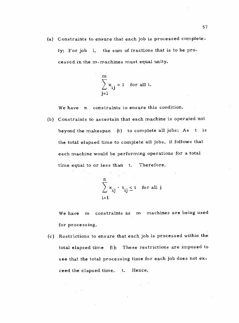
(a) Constraints to ensure that each job is processed complete-

ly: For job i, the sum of fractions that is to be pro-

cessed in the m- machines must equal unity.

x.. =1 for all i. 1J

j =1

We have n constraints to ensure this condition.

(b) Constraints to ascertain that each machine is operated not

beyond the makespan (t) to complete all jobs: As t is

the total elapsed time to complete all jobs, it follows that

each machine would be performing operations for a total

time equal to or less than t. Therefore,

n x,. t..<t for all j 13 13 -

i=1

We have m constraints as m machines are being used

for processing.

(c) Restrictions to ensure that each job is processed within the

total elapsed time (t): These restrictions are imposed to

see that the total processing time for each job does not ex-

ceed the elapsed time, t. Hence,

[m)'

m t, < t for all i. aj-

j=1

58

We have n constraints to ascertain that this property is

satisfied over all jobs.

The objective function is to minimize the total elapsed time:

minimize z .=

As all the x, ,'s and t..'s are non -negative values, 1J

xij, tij, t > for all i and j.

Hence for a problem of m machines and n -jobs, we have a linear

programming model with (mn +1) decision variables.

Example: The following three jobs are to be scheduled on two

single stage. facilities. The processing times, t, are are given in the iJ

Table 2 -32. The objective is to minimize the makespan. The split-

ting of jobs is permissible.

Table 2 -32. Processing times for jobs on 'non- alike' machines.

Job, i Machine, j

1 2

1 6 7. 8

2 3 3.6 3 10 11

x..

0 13 13 -

si

,

59

The linear programming model may be formulated as following:

Minimize:

Subject to:

Set (a):

Set (b):

Set (c):

z = t

x11 + X12 = 1

x21 x22, = 1

x31 + x32 = 1

6x11 +3x21 +10x31 <t

7. 8x12 + 3. 6x22 + 11x32 < t

6x11 +7.8x12 <t

3x21 + 3. 6x22 < t

10x31+ 11x32 < t

x.., t > 0 for all i and j. 1

We note that there are 7 decision variables in the model. The

computation yields the following values in the final iteration.

x11 = 0. 597

0. 403 x12 =

x21 =0

x22 = 1. 000

x31 = 0. 674

x32 = 0. 326

+

-

and

tW10.326

60

It may be observed that job 2 is processed only in machine 2.

It is not required that each job is able to be processed in all

facilities. If a job i cannot be processed in facility j, we may

ignore the assigning of i in j, that is x.. = O. We shall illus-

trate this situation by a simple example.

Example: Four jobs, J1, J2, J3 and J4, are to be se-

quenced on two single -stage machines, M1 and M2. If splitting

is allowed, in which order should the production planning manager

assign the jobs so that the makespan (days) is minimized. J2 can-

not be processed in M2.

Table 2 -31. Processing times for jobs on 'not -alike' processors.

Machines, j Jobs, i Ml M2

J1 5 8

J2 7 --®

J3 6.5 9.7

J4 3.3 1.1

The linear programming model may be formulated as follows:

Minimize: z = t

Subject to:

61

xi1 + xi2 1

x 1 21

x31 + x32 = 1

x41 + x42 = 1

5x11 + 7x21 + 6. 5x31 + 3. 3x41 < t

8x12 + 9. 7x32 + 1. lx42 < t

5x11+8x12<t

7x21 < t

6. 5x31 + 9. 32 7x32 < t

3. 3x41 + 1. 1x42 < t

x.., t > 0 for all variables in 13 -

the model.

On solving the problem, we obtain the following values:

x1 = 0. 907692

x12 = 0. 092308

x21 = 1

x31 =0

x32 = 1.

x41 =0'

x42 = 1.

t = 11. 5385

=

62

The total elapsed time is 11. 5385 days and it may be shown on the

Gantt chart in many ways (as the jobs can be split).

For a problem of n tasks to be sequenced in m machines,

there would be (mn +1) decision variables and (m +2n) restric-

tions. Thus, for 20 tasks in 10 machines, we shall have 201 dicision

variables and 50 restrictions.

The first example problem required 12 iterations using the two -

phase method and used 31. 67 cpu seconds for computation and execu-

tion of the LINPRO program on a General Electric 265 time - sharing

system. The second example took 28.83 cpu seconds and required

11 iterations.

63

III. SINGLE STAGE - -SETUP TIME SEPARATED FROM PROCESSING TIME

When the setup times and the working times are separately

given for tasks processed in a single stage production facility such as

an automated steel section production line, the makespan (elapsed

time) can be computed as the sum of the setup times and the process-

ing times.

Normally the setup time is dependent on two factors, 1) the

time required to dismantle the previous setup and 2) the time re-

quired to arrange the machine for the new job. In otherwords, the

setup time varies according to the job previously processed and the

new job to be processed after it is ready. The setup times are usu-

ally given in an n x n square matrix, where t.. denotes the setup 1J

time to make ready the facility for job j after processing job i.

The processing time of a job is usually independent of the order

in which the tasks are sequenced on the facility. The time required

to process job i is represented by ti .

A. Elapsed Time

We note that the total elapsed time is the sum of setup times and

the processing times.

Let us consider the schedule of n jobs in the numerical

order, that is, 1, 2, 3,... , n. Then,

Total make span, T = ti + (t12 +t23 +t34 + ... +t

12 i=1

)

64

Minimizing the makespon is the same as minimizing the sum of setup

times, since the sum of processing times is a constant regardless of

the order in which the jobs are arranged. If the factory is manufac-

turing a set of n jobs repetitively;: the computational method for

determining the optimal schedule that minimizes the make span is the

same as the one used to solve a travelling salesman problem.

Little, Murty, Sweeney and Karel (1963) have developed an

algorithm (branch and bound technique) for the travelling salesman

problem. Of all the presently available methods to solve this prob-

lem the branch- and -bound algorithm appears to be the most success-

ful method as it requires comparatively less computation.

An open -path problem is a single stage n -job problem where

the last job already scheduled is known and a set of ( _1) jobs

which are not repetitive are to be processed subsequently on the

same single stage processor. Gavett (1965) has presented three

heuristic rules for this open -path case and his computational experi-

ence on these rules. We shall also in the section, present our formu-

lation of an algorithm for an open -path case to determine the schedule

that will minimize the total elapsed time. This method is based on

the 'branch and bound technique' of the travelling salesman problem.

65

1. A Set of Repetitive Jobs -- Travelling Salesman Problem (Closed Path Scheduling)

The travelling salesman problem may be stated as follows. A

salesman is to visit n cities. His routing must start from a city,

and include a visit to each of the remaining (n -1) cities once and

only once and return to the start. To minimize the total distance

travelled, in what order should he visit the n cities?

For a single stage scheduling problem we can paraphrase the

problem by using, "setup time" instead of 'distance' and 'job' instead

of 'city.' It is to be noted, however, that in a travelling salesman

problem, the distance from city i to city j is the same as from

city j to i, whereas in a single -stage production scheduling

problem the changeover time (setup time) for the machine from job i

to job j is not necessarily the same as from j to i.

Table 3 -1. Setup times, t.., for n jobs.

2 3 4 .. n

1

2

3

4

00

t21

t31

t41

tnl

t12 00

t32

t42

tn2

t13 t23

00

t43

tn3

t14

t24

t34 00

tn4

tln t2n

t3n

t4n

00

i J

1

' .

'

"

. "

n "

There is only one job of each type in the set of n jobs and

hence, t.. = oo. The setup times can be arranged in a tableau as

66

shown in Table 3 -1. We are to choose n elements, one in each

row and one in each column, so that the sum of the elements chosen

is minimized. We must also take care to guarantee that the machine

is made ready to process each job only once and the machine is ar-

ranged to process the first job only in the n -th changeover.

Initially we may treat the salesman problem as an assignment

problem and check if the solution satisfies the restrictions (M. Sasieni,

A. Yaspan and L. Friedman, 1959).

An algorithm for the assignment problem is as follows

(Fredrich S. Hiller and Gerald J. Lieberman, 1967):

Step (1): Enter the setup times, t.. in in the square matrix of size

Place t.. = oo for i = 1, 2, . . . , n. ii

Step (2): Find out the minimum element in each row and subtract it

from every element of that row. Then, reduce each column,

if possible, in the same way.

Step (3): Check the rows and columns successively. For each row or

column with exactly one zero,element, we choose the posi-

tion for assignment and the other zero element positions in

that row or column are eliminated.

Repeat the same procedure till all the zero element po-

sitions are either assigned or eliminated. If we can assign

n.

it

67

one zero in each row and one zero in each column, we have

obtained a solution. Otherwise, we shall proceed with the

next step (4).

Step (4): Draw a minimum number of lines (equal to the number of

assigned zero positions) to cover all zero elements.

Step (5): Find out the minimum of the elements that are not covered

by the lines drawn in Step (4). Subtract it from the uncov-

ered elements and also add it to each element that is situated

at the intersection of two lines. Go to Step (3).

We shall illustrate the algorithm by a simple example:

Table 3 -2. Setup time matrix [t..] for six jobs. 1J

1 2 3 4 5 6 Subtract

y

1

tI00 14 19 13 13

8 00 3 5

25 18 00 27 7 25 23 00 19

11 13 4 0 00 0

Subtract by 3

Table. 3 -3. Scheduling the jobs using the method for assignment problem.

i

J 2 3 4

1 00 12 0 0 4 2 1 0) 00 9 3 3

3 8 5 2 6

4 10 18 8 00 20 5 11 15 16 00 12 6 12 11 10 4 Ell CO

r",- denotes the positions assigned.

00 29 20 17 17 21 17

2 10 10

3 11 9 3

4 17 7 7

5 18 7

6 21

1 5 6

I Of 1

co © n 0

l

68

For this, we note that the production schedule is 1- 3- 4- 6- 5 -2 -1.

This satisfies the restrictions of the travelling salesman problem and

so this is the optimum schedule with an elapsed time of 47 time units.

All the travelling salesman problems cannot be solved by the

assignment solution. In such cases, the branch and bound technique

developed by Little, Murty, Sweeney and Karel will be useful.

We shall describe some remarks about the algorithm before

presenting the algorithm for determining the optimum schedule.

Let

T = = [t(i, j)] = processing time matrix.

s = path (schedule) represented by a set of n ordered job

pairs, like (in -1,

This forms a closed path processing each job once and

only once.

Z(s) = time required for the schedule s

(i, j) in s

t(i, j)

X, Y, Y = nodes of the tree.

v(X) = a.lower bound on the total time required of the schedules of

X. Or in otherwords Z(s) > v(X) for s, a tour of X.

Z0 = the time elapsed for the best schedule determined so far in

the algorithm.

[(il, i2)(í2, i3)(í3, i4)... in)(in, it )j

=

69

Reducing the Time Matrix and the Lower Bounds: If we sub-

tract a constant, r, from each element of a row of the time matrix,

the total time required for any schedule under the revised matrix is

less by r than the original matrix. The relative times of all other

schedules are not changed and so any schedule that is optimal for the

original matrix will also be optimal for the revised matrix. The

method of subtracting the smallest element from each row is known

as reducing the row, and similarly, the process of subtracting the

smallest element from each column is called reducing the column.

A reduced matrix is obtained by reducing the rows and columns so

that all the elements are non -negative and there is at least one zero

in each row and each column. Then,

Z(s) = r + Z1(s)

where

Z(s) = the time required for a schedule s before reducing the

matrix.

Z1(s) = the time required for the same schedule s after reduc-

ing the matrix.

r = sum of the constants used in reducing the matrix over all

rows and columns.

As all elements in the reduced matrix are non -negative with at least

one zero in each row and column, we require at least r time units

70

to complete any schedule under the old matrix. We can not find a

schedule for the old matrix with elapsed time less than r, which is

said to be the lower bound of the old matrix.

Branching: The set of schedules are split into disjoint subsets

and are being represented by the branching of a tree as shown in Fig-

ure 3 -1.

All schedules

Figure 3 -1. Start of the branching of tree.

The branching of the tree starts with the node, 'all schedules.'

This is branched into two subsets, one being the node (c, d) rep-

resenting all the schedules that include the job pair c, d and the

other node (c, d) showing all schedules that do not contain (c, d).

The branching from (c, d) contains m, n and m, n. The node

m, n represents all schedules that contain (c, d) but not (m, n)

71

and the node (m, n) indicates those schedules containing (c, d) and

also m, n. By tracing from a node, X to the starting node, we

can determine the job pairs chosen to appear in the schedule and

those that are not.

In branching out from a node X into two nodes, the node with

the newly chosen pair is called Y and the node with the forbidden

schedule pair is called Y in the algorithm.

Algorithm:

Step (1): Obtain the reduced setup time matrix, [t! .] . Let S = 1 iJ

be the set of all possible schedules. Label S with

v(S) = sum of reducing constants.

Step (2): For each cell (a, b) with zero time in the reduced matrix

[ti.] compute the penalty (pa b) of not using it, where s

(p ) = min [t!.] + min [V.] a,b i #a J 1 1J

J #b

Enter the value of (pa, b) in the cell (a, b) as shown in

Table 3 -7.

Step (3): Choose a cell (c, d) such that pc = max (pa b) for all

a and b values. Ties, if any, may be broken arbitrarily.

We branch the set of all possible schedules from S into

those that contain the path (c, d) and those that do not.

Let us denote these subsets by Y and Y. Delete row c

J

72

and column d.

Step (4): The lower bounds for the subsets Y and Y may be cal-

culated as follows: For the subsets Y, v(Y) = v(S) + p c, d

determine the starting job s and the ending job e of the

schedule containing (c, d) among schedules generated by

the selected pairs of Y. Record in the matrix [t!j],

t(e, s) = oc, Reduce the matrix [t!.], if possible for the iJ

subsets Y, v(Y) = v(S) + (sum of reducing constants).

Step (5): Check if the reduced matrix is of size 2 x 2. If yes, com-

plete the single tour and continue. Otherwise, go to the next

step (6).

Step (6): Examine the lower bounds of the nodes obtained so far and

choose the one with the smallest value.

Step (7): Check if the best schedule found so far has an elapsed time

(Z0) less than or equal to the lower bounds on all terminal

nodes of the decision tree. If yes, the sequence established

in Step (6) is the optimal schedule.

If the lower bound of some other arbitrary node X

has less value than that of the last node Y, go to Step (8).

Otherwise, go to Step (2).

Step (8): In the original setup time matrix [t..], choose the pairs iJ

(c, d) that are previously selected in the tour of S. Com-

pute g = /tc, d.

73

For each of (c, d), delete the row c and column d.

For each path among the (c, d) group, find the starting

job s and the ending job e and set t (e, s) = 00. For

each (c, d) that is not included in the schedules of S,

set t(c d) Reduce the remaining matrix [t..), if

possible.

The lower bound of X, v(X) = g + sum of reducing con-

stants. Then, go to Step (2).

Example: The production planning engineer of a printing press

has one press for printing six monthly magazines. The sum of print-

ing time in the press is estimated to be 240 hours each month. If the

machine is available for 300 working hours (for changeover and

printing) each month, the engineer wishes to know if these six repeti-

tive jobs (magazines) can be completed within the available regular

time. The setup time matrix (in hours) is shown in Table 3 -4.

Table 3 -4. Setup time matrix for the printing press problem.

1 2 3 4 5 6

1 00 10 12 21 18 14

2 10 00 11 28. 7 24 3 11 13 00 14 16 12

4 17 9 16 00 35 13

5 18 21 8 11 00 9

6 12 14 10 9 21 00

= 00.

N

74

The algorithm for assignment problem yields the final reduced

matrix as shown in Table 3 -5. This is not a feasible schedule for the

single -stage scheduling problem (repetitive set of jobs) and hence

using the algorithm for the sequencing problem for the set of repeti-

tive jobs, we can establish the optimal schedule.

Table 3 -5. Schedule obtained by the method for assignment problem.

1 2

1 00 0

2 3 00

3 01 4

4 8 M 5 10 15 6 3 7

3 4 5 6

ED 9 6 1

16 4 21 00 3

7

0 3

01

5 0

00 26 3

00

I

1 IOf 12 00

Li- denotes positions assigned. Schedule obtained: 1-3-1, 2-5-6-4-2.

We obtain the intermediate reduced setup time matrices as

shown in Tables 3-6 to 3-11.

Table 3 -6. The reduced setup time matrix No. 1.

\i

1 2 3 4 5 6

1 00 0 2 11 8 3

2 3 00 4 21 0 16

3 0 2 00 3 5 0

4 8 0 7 00 26 3

5 10 13 0 3 0o 0

6 3 5 1 0 12 00

\ []

\

75


i

.i 1 2 3 4 5 6

1 00 0® 2 11 8 3

2 -3 3 co 4 21 0--16 0

3 0® 2 co 3 I o®

4 8 0® 7 ;; ao 26 3

5 10 13 0® 3 Ç o©

6 3 5 1 0® 1

1 2 co

I

Table 3-8. The reduced setup time matrix No. 3.

i

J 1 2

1 °O 0®

3 0Q 2

4 8 0® 5 10 ao

6 3 5

3 4

2 11 3

co 3 0 7 3

OQ 3 OO

1 ------p 00


6

3 6

2 3

co 0© 7 co

OC) 0 ®

\ Z

1 00 3 --00- 2

4 8 OO

5 10 m

55

All schedules

55

58

Optimum schedule 1- 6- 4- 2 -5 -3 -1

Optimum value = 58 hours 58

76

Figure 3-2. The final tree for the optimum (closed path) schedule.

77

Table 3. 10. The reduced setup time matrix No. 5.

4

5

2 3 6

10® O 00 3

10®

I

Oo

Table 3. 11. The reduced setup time matrix No. 6.

6

1 00

5 0® 00

We have established the optimal schedule for the six (repetitive)

jobs in the press. It requires 298 hours (= 58 + 240) for the comple-

tion of the tasks in each month on regular time.

2. A Set of Non -Repetitive Jobs

(a) Heuristic Rules. Gavett (1965) has developed three heuris-

tic methods for choosing a schedule for the single -stage sequencing

problem and presented his experimental results on these computa-

tional methods.

We shall describe the three rules with the aid of a simple nu-

merical example.

\ 1

7

00 OO i

i 3

0®

78

Example: Five jobs are to be processed by a milling machine.

Job J1 has just been completed, and J2, ... , J6 are ready to be

processed. The five jobs are to be sequenced to minimize the make-

span for the machine. The setup times, t.. (hours), for the jobs

are given in Table 3 -12.

Table 3 -12. Setup times for jobs on a milling machine.

\\` J 1 2 3 4 5 6

1 0o 29 20 17 17 21 2 00 00 14 19 13 13 3 0o 8 00 3 5 9

4 0o 25 18 co 27 7

5 00 7 25 23 00 19 6 0o 11 13 4 0 00

Using the algorithm for open path (Chapter III- Section A- 2b),

we can determine the optimal schedule 1- 3- 4 -6 -5 -2 and the optimal

value (T) is 37 hours.

The three heuristic methods presented by Gavett are

(i) the "next best" rule (NB)

(ii) the "next best prime" rule (NB')

and (iii) the "next best double prime" rule (NB ").

(i) Next Best Rule: The method is to choose the unassigned job

which has the least setup time relative to the job that has just been

completed. For our example, we would obtain the two schedules:

rl

79

(a) 1-4-6-5-2-3 (T = 45)

(b) 1-5-2-6-4-3 (T = 59)

The two sequences resulted from a tie in choosing job 4 or 5 after

completing job 1.

(ii) Next Best Prime Rule: In this method, after completing the

first order -position job (J1), we assign each of the remaining

(n -1) jobs in turn in the order - position 2. For establishing the jobs

in the order -positions 3, 4 and so on, the NB rule is used. By

this rule, we establish at least (n -1) sequences and choose the one

with the least elapsed time.

The NB' rule yields also the schedule resulting from NB

rule as one of the sequences and hence, by the NB' rule we can

obtain a schedule which is at least as good as the sequence yielded

by the NB rule.

sequences:

For our example, we obtain the following six

(1) 1_2- 5 -6 -4 -3 T = (83 hours)

(2) 1- 2- 6 -5 -4 -3 T = (83 hours)

(3) 1- 3- 4 -6 -5 -2 T = (37 hours)

(4) 1- 4- 6 -5 -2 -3 T = (45 hours)

(5) 1_5- 2 -6 -4 -3 T = (59 hours)

(6) 1_6- 5 -2 -3 -4 T = (45 hours)

Of these six schedules, we select (3) in accordance with the NB'

80

rule. This rule is also known as the next best rule with variable

origin.

(iii) Next Best Double Prime Rule: In this method the NB

rule is applied after subtracting the minimum value in each column

of the setup time matrix from each value in the column. The matrix

after the column reduction is shown in Table 3 -13 for our example.

Table 3 -13. Matrix after column reduction.

1 2 3 4 5 6

1 00 22 7 14 17 14 2 o0 00 1 16 13 6

3 o0 1 o0 0 5 2

4 o0 18 5 00 27 0

5 o0 0 12 20 00 12

6 00 4 0 1 0 o0

The application of the NB rule to the reduced matrix yields

the schedule

1- 3- 4 -6 -5 -2 ... (T = 37 hours).

This method is also known as the next best rule after column reduc-

tions.

For the experiments, the setup times have been generated from

a known distribution type with given mean and variance. It has been

found that for problems with normally distributed setup times the

average percentage increase in elapsed time over optimum was 10%

for the NB rule and 6% for the NB' rule. Therefore, we may

i \

81

conclude that the NB' rule yields a better schedule than the NB

rule. However, we note that NB' rule required more computation-

al effort than that for NB rule.

Investigations on problems with unformly distributed setup

times show that the use of NB" rule results in some gain in effi-

ciency over the other two rules. In this situation, the average ratios

of the elapsed time by the NB" rule, NB' rule and NB rule

to the optimum value were found to be 1. 25, 1. 34 and 1. 57 respec-

tively.

For large size problems, if the computing facilities are not

available, these heuristic methods may be applied to determine a

sequence without too much computation.

(b) Application of Branch and Bound Technique. In many in-

dustrial situations, a set of tasks must be scheduled for processing

in a facility that is still processing a task from the previous schedule.

In the following production period, the next set of jobs, including the

one still being processed are to be sequenced for processing in the

same machine so that the total elapsed time (processing times plus

setup times) for the machine is minimized. This may be conceived

as an open path scheduling problem for a set of non - repetitive jobs.

We have described the heuristic methods by Gavett (1965) in the pre-

vious section. We shall now present our own computational method

for establishing the optimal sequence for the n- non -repetitive jobs on

82

a single -stage (machine). The criterion is to minimize the total

elapsed time which is equivalent to minimizing the sum of setup

times.

The scheduling problem for a set of non -repetitive jobs may

be stated as follows:

There are a set of n non - repetitive jobs to be scheduled on a single -stage production facility during the production period, k. If job d is the last one which was processed in the period (k -1) in the facility, in which order must the n -jobs be sequenced so that the make - span is minimized?

For the sake of simplicity in describing the computational

method, let us suppose that job d = job 1 and the n -jobs be num-

bered 2, 3, ... ,n,(n +1). The setup times may be represented in the

matrix form (T) as shown in Table 3 -14.

T =

Table 3 -14. Setup time matrix for the open -path scheduling problem.

i 2 3 ... n (n+1)

1

2

3

n

0o t12 t13 tln t tl(n+l) 0o 0o t23 . t2n t2(n+l) 0o t32 00 t3n t3(n+l )

tn2 tn3 0o tn(n+1)

t(n+1)2 t(n+1)3 t(n+1)n oo

There is only one job of each type and hence we cannot process

job i after processing job i. This is avoided by setting t.. = 00

1

00 "'

(n+1) 00

'

83

(Table 3 -14). Also we note that the facility need not be setup for job

d (job 1) again in period k and therefore, til = oo . The setup

time matrix [t..] may also be constructed of size (n +1) x n in iJ

which the column for job 1 of the original (n +l) x (n +l) size matrix

is ignored. Let this (n +1) x n matrix be denoted as T'.

Let us also consider the feasible sequence S, in which the

tasks are processed in their numerical order.

S = 1-2-3-4- . . . -n-(n+1).

We note that after completing job 1, we must rearrange setup of the

facility n more times (corresponding to n rows of which i = 1

is one. The schedule must consist of i = 1 and of any other (n -1)

rows of the remaining n rows). In our example, the rows to be

considered are i = 1, 2, 3, ... , n.

We are arranging the facility n times (corresponding to all

the n columns of matrix T). In our example, therefore, the col-

umns to be considered are 2, 3, 4, ... , n, (n +1).


Step (1): Construct the setup time matrix T of size (n +1) x n as

shown in Table 3 -15 and enter all the t.. values. 1J

84

Table 3 -15. Setup time matrix for a set of non- repetitive jobs.

2 3 ., n n+1

1 t12 t13 tin 1(n+1)

2 0 0 t23 . t2n t2(n+1)

3 t32 00 t3n t3(n+1)

n tn2 tn3 ... o0 tn(n+1) n+1 t(n+1)1 t(n+1)2 t(n+1)n

o0

Step (2): Add a slack (or dummy) column (n +2) and assign the value

ti(n +2) = 0 for i = 1, 2, ... , (n +1). Apply the algorithm for

the assignment problem (described in Chapter III -Section

A -1) and determine the optimal assignment. Check if it is

a feasible sequence. If it is a feasible schedule, the values

obtained are for the optimal sequence and the problem is

solved. If not, go to Step (3).

Step (3): Apply the algorithm to the scheduling of a set of repetitive

jobs which is now a travelling salesman problem (described

in Chapter III -Section A-1) for the setup time matrix T in

Step (1) and establish the optimal schedule. In using the

above algorithm, the following changes are to be incorpo-

rated: whenever reducing the matrix, all the n columns

and only the row corresponding to i = 1 are to be consid-

ered.

"'.

85

Note: Of the remaining n unreduced rows, we shall be choosing any

(n -1) of them. If all the n unreduced rows are considered

for row reduction, the lower bounds obtained in that situation,

do not represent the true lower bound values. Therefore, only

(n -1) rows are taken into account for row reduction.

The schedule obtained is the optimal sequence.

Example: The foreman of a forging section has received five

new orders to be filled that require processing in a drop forge during

the month of April. The last job that is already scheduled to be in-

process in the machine in March is job 1. In which order may the

five new jobs (2, 3, 4, 5, 6) be scheduled for production so that the

makespan is minimized? The setup time matrix (hours) is shown in

Table 3-16.

Table 3-16. Setup time matrix [t..] for 13

jobs in a forging section.

2 3 4 5 6

1 29 20 17 17 21 2 00 14 19 13 13 3 8 00 3 5 9

4 25 18 00 27 7

5 7 25 23 00 19 6 11 13 4 0 00

For using the algorithm for the assignment problem, a slack

column (j = is to be added as shown in Table 3 -17.

86

Table 3 -17. The initial setup time matrix for using the method for assignment problem.

2 3 4 5 6 7

1 29. ' 20 ,/ 17'' 17 21 ''r 0

2 00 14 ' 19 13 13 4 0

3 8; 00 3 o 5 9ü 0

4 251 18 00 27 7 0 0

5 7 t: 25 n- 23 -:.) ao 1.9 h- 0

6 11 w; 13 0 4 k 0 00 0

The optimal assignment is denoted in Table 3 -18. But, this is

not a feasible schedule. Therefore, we apply the open -path algorithm

to a set of repetitive jobs for the matrix [t..] of Table 3 -16. The iJ

intermediate reduced matrices are shown in Tables 3 -19 to 3 -24.

Table 3 -18. The optimal assignment matrix.

N 2

1 21 2 00

3 1

4 18 5 I 01 6 4

3 4 5 6 7

6 13 16 13 Ulf

D 15 12 5 0

oo a 5 2 1

5 o0 27 1 01 1

12 20 00 12 1

0 1 I OÍ 00 1

=1- denotes positions assigned.


2 3 4 5 6

1 15 0 7 10 7

2 00 1 16 13 6

3 1 o0 0 5 2

4 18 5 00 27 0 5 0 12 20 00 12 6 4 0 1 0 00

\J

::

87

Table 3 -20. The reduced setup time

J 2

I

1 15

2 i I

3 1

4 .18

matrix No. 2.

3 4 5 6

00 7 10 7

1 16 13 6

0o OC) 5 2

5 00 27 00 5 D 12 20 00 12

6 4 OC) 1

I


i J 6

1

2

0` 1

7

16

10

00

7

6 I

3 0o 0 ® 5 2 I

4 5 00 27 0

6 00 1 0®

Table 3 -22. .. The reduced setup time matrix No. 4.

J 4 5

OO 7 10

2

3

6

1 16 00

b e 5 _co OO 0! 00

i

0O 00

3 4 5

l0

3 i

1

I

I

I

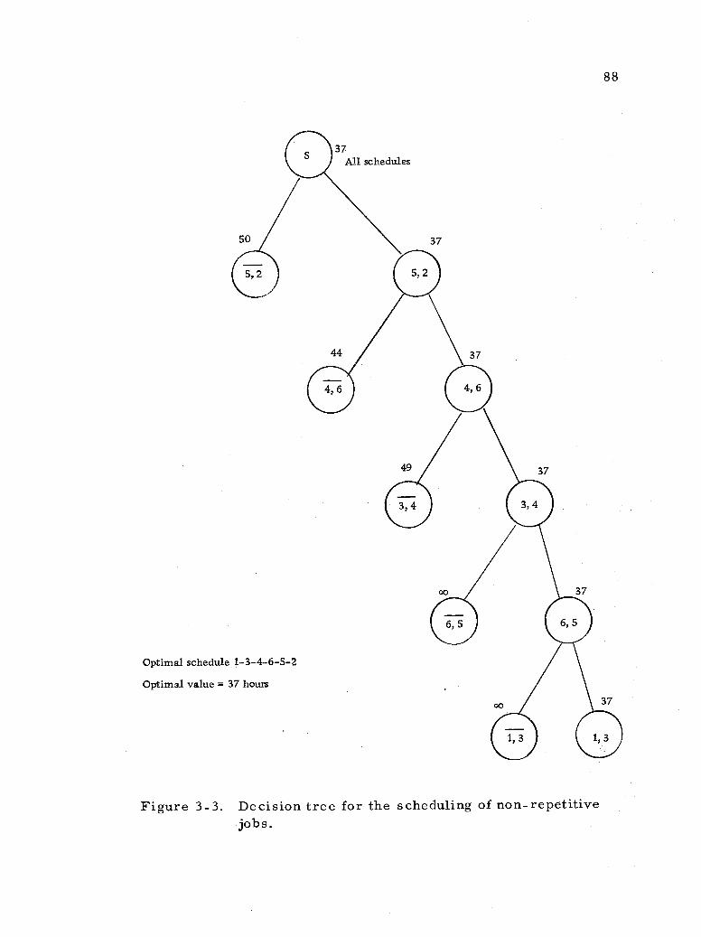
37 All schedules

37

37

37

88

Optimal schedule 1- 3- 4 -6 -5 -2

Optimal value = 37 hours

Figure 3 -3. Decision tree for the scheduling of non - repetitive jobs.

89


3 5


1

2

From the decision tree (Figure 3 -3), we obtain the optimal

schedule 1- 3- 4 -6 -5 -2 and the optimal value is 37 hours.

We believe that this open -path algorithm offers an alternative to

the three heuristic rules by Gavett (1965) presented earlier in the

preceding section.

i

1

2

6

0© I

CO

10

00

J

i 3

o

90

IV. TWO- STAGES - -SETUP TIMES INCLUDED WITH PROCESSING TIMES

In some manufacturing situations, the products may require

processing in two stages, say A and B. From a technological

point of view, the processing in A and B may have been defined

in which order the job is to be processed. For example, the job must

be degreased first and only then can it be painted.

Ignall and Schrage (1965), Johnson (1954) and Mitten (1959) have

presented algorithms to determine the optimum schedules in different

situations assuming that each job is first processed in machine A

and then in B. Jackson (1956) has formulated a computational meth-

od wherein the scheduling of the job in all possible ways (first A

then in B, first B and then in A, only in A and only in B)

are considered.

It is also assumed that there is only one of each type of machine

(A and B) and that the setup time of each job is independent of the

order in which it is processed and included with its processing time.

A. Completion Times - -Sum of Completion Times

Ignall and Schrage (1965) have developed an algorithm for min-

imizing the mean of completion times for a two stage production

scheduling problem. Each job is first processed in facility A and

then is facility B. The computational method is based on the branch

91

and bound technique of Little, et al. (1963).

For a given problem, minimizing the mean of the completion

times of the jobs is equivalent to minimizing the sum of completion

times.

Let

a. = processing time on machine A for job i

b. = processing time on machine B for job i

c. = completion time of job i (on machine B)

Sr = a particular schedule of r jobs from the given job set

1, 2, 3,..n

f = the last job in the schedule Sr

Sr = jobs that are included in the given job set 1, 2, 3, ... ,n but

not in Sr. r

i1, i2, 3

. . , in-r

and is arranged so that

j2,...,jn_r

ranged so that

is a sequence of the jobs in the set S

a, < a. < a. . . . < a. . 11 ® 12

13 = n-r

is a sequence of the jobs in the set Sr

b. < b. < b. ... < b..

J1 = 32 = 33 = 3n-r

and is ar-

We shall consider any schedule with Sr as its first r jobs.

= in_

r

r

i3, -r r

92

The remaining (n -r) jobs are to be scheduled in the last (n -r)

order positions. The sum of completion times can be divided into

two groups as

c. + 1

lEfS r 1Eg r

c.. 1

We wish to obtain a lower bound for the second sum.

Kr =

n-r

P=1

a.+(n-r-p+l)a. +b. 3 1p 1p

j E Sr

n-r - Lr = max (c, a.+min- a. )+(n-r-p+1)b.

J J Sr 1 Jp

p=1 - jE Sr

where Kr is the sum of completion times of the jobs in Sr when

they are processed in the order i1, i2, . 1n_r and if the process-

ing times on A dominate and also Lr refers to the same sum

when the jobs are processed in the order

processing times on B dominates.

Then,

lower bound for (S ) = r iE Sr

Algorithm:

J2' , in-r

ci + max (Kr, Lr).

and if the

Step (1): Consider that the n jobs may be scheduled in the first

r

r

r

,

-

j1,

/

93

order position. Taking each one of them in turn, compute

the lower bound. Compare the lower bounds and choose the

least of them. This is represented in the decision tree as

shown in Figure 4 -1. Let the chosen node be k.

Step (2): With the job k in the first order position, the remaining

(n -1) are considered for being scheduled in the second

order position and their lower bounds are calculated. Ex-

amine the least of the lower bounds and construct (n -2)

branches (if the branching is from the second order position)

or (n -1) branches (if otherwise) and calculate their lower

bounds.

Repeat the same procedure till the n -th order position has

been assigned.

Compare the least of the lower bounds of the last stage with the

values of the previous levels. If it is not greater than the remaining

lower bounds, this schedule gives the optimum order of jobs for mini-

mizing the sum of completion times. If not, from the node with a

lesser lower bound value, branch out further in a similar way and de-

termine the optimum sequence.

We shall illustrate the algorithm by a numerical example.

Example: The production planning engineer of a textile mill is

asked to schedule four jobs so that the mean of their completion times

94

is minimized. Each job consists of two stages. In the first stage,

the fibers are converted into a basic thread yarn and in the second

stage it undergoes dyeing.

Node (1):

Table 4 -1. Job list of a textile mill.

Processing time in days Job No. A B

1 10 12 2 8 7

3 6 4 4 5 9

Kr = [10+(5x3)+9] + [10+(6x2)+4] + [10+(8xl)+1]

= 85

= [max(22, 10+5)+3x 4] + [22+(2 x 7)] + [22+(1 x 9)]

= 101

Lower bound = 22 + max (85, 101)

= 123 days

Similarly we compute the lower bounds for nodes 2, 3 and 4 and enter

the values in the decision tree (Figure 4 -1). We note that node 4 has

the least value and hence branch out the nodes 41, 42 and 43.

Node (41):

= [15+(6x2)+4] + [15+(8x 1)+7]

= 61

Lr

Kr

95

103 98 109 101

Figure 4 -1. Decision tree.

96

= [max (27, 15 +6) +4x 2] + [27 +7x 1)

= 69

Lower bound = (14 +27 + max (61, 69)

= 110 days.

Similarly we calculate the lower bounds for the nodes 42 and 43 and

enter in the decision tree. We branch out from node 42 as it has the

least lower bound.

Node (421):

Kr = 23+6+4=33

Lr = max (35, 23 +6) + 4 = 39

Lower bound = (14 +21 +35) + 39 = 109 days.

In the same way, we compute the lower bound for the node 423.

Examining the lower bounds we observe that the node 3 has the

least value. Hence, we compute the lower bounds for the nodes 31,

32, 34 and then for 341 and 342.

From the decision tree, Figure 4 -1, we note that the schedule

342 has the minimum lower bound and therefore, this is the optimum

schedule. This is shown in the Gantt chart, Figure 4 -2, and the

mean of completion times is 94 = 22. 5 days.

Lr

B

(3) (4) (2) (1)

t\\\\\ \\17////J r _-- --- --- 1\zl.tüli

n\\\ %/!// 11101cIMIMIZIM 'WOW

20 30 40 50 10

97


B. Elapsed Time

The total elapsed time for a two stage job -shop scheduling prob-

lem is the time from the beginning of the first job in machine A or

in machine B (whichever is earliest) to the completion of the last

job in machine A or in machine B (whichever is the latest). The

objective is to minimize the total elapsed time.

Johnson (1954) has established a computational method for de-

termining the optimal schedule when all the jobs are processed in

machine A first and then in machine B.

Mitten (1959, 1959) has formulated an algorithm for obtaining

the optimal schedule when each job has one start and one stop timelag.

He has considered two cases, (1) for each job the start timelag and

the stop timelag are not equal, (2) for each job the start timelag and

98

the stop timelag are equal. The algorithm is fomulated on the as-

sumption that each job is processed first in machine A and then in

machine B.

The Johnson's Rule (1954) has been extended to joblots in which

few jobs may require processing in machine A only, some jobs

require processing in B only, some tasks require processing first

in A and then in B or in the other way about. This method pre-

sented by Jackson (1956) is likely to require more in- process storage

facility than the original Johnson rule's application.

1. Johnson's Method

An example of a two -stage problem can be presented as follows:

A book binder has one printing press and one binding machine. He

has manuscripts for different books. The times required to perform

the printing and binding operations for each book are known. The

foreman wants to establish the order in which the jobs (books) are to

be processed, in order to minimize the total time required to com-

plete all the books. In this case, each job requires processing in two

machines (two stages) - -first in the printing press (A), then in the

binding machine (B).

Johnson (1954) has formulated an algorithm for determining the

optimum schedule for this type of two -stage problem. The detailed

proof can be found for this algorithm in Johnson (1954).

rule:

99

Certain assumptions are necessary for the application of this

Assumptions regarding machines:

1. No machine may process more than one job at any given

time and each job, once started, must be processed to

completion.

2. The exact or expected processing times are known. The

time intervals for processing are independent of the order

in which the operations are performed. The setup times

are included with the respective processing times.

Assumptions regarding jobs:

1. All jobs are known and are ready for processing before the

period under consideration begins.

2. All the jobs are considered equal in importance, that is,

there is no priority among the jobs.

3. Jobs are processed by the machines as soon as possible and

in the same order on both machines.

4. No job can be processed at any given time in more than one

machine.

5. Each job is processed first in machine A and then in

machine B.

Other assumptions:

1. In- process inventory is allowable.

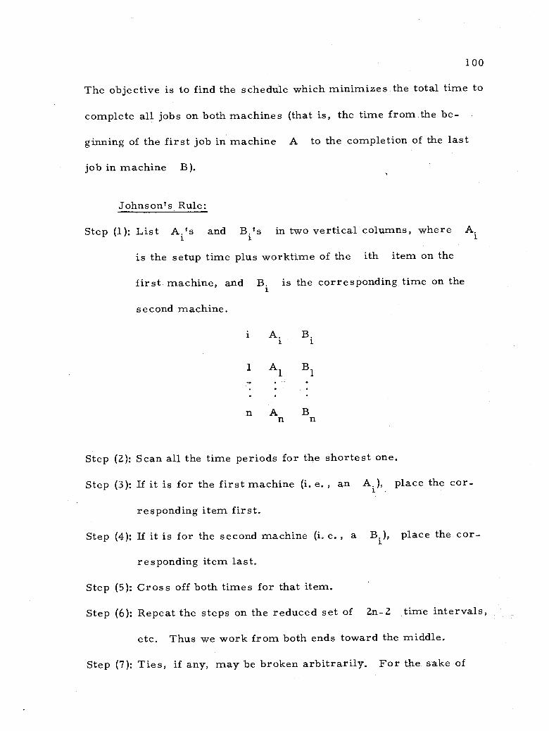
100

The objective is to find the schedule which minimizes the total time to

complete all jobs on both machines (that is, the time from the be-

ginning of the first job in machine A to the completion of the last

job in machine B).

Johnson's Rule:

Step (1,): List A.'s and B.'s in two vertical columns, where A.

is the setup time plus worktime of the ith item on the

first machine, and B. is the corresponding time on the

second machine.

i

1 Al

B. i

n A B n n

Step (2): Scan all the time periods for the shortest one.

Step (3): If it is for the first machine (i. e. , an Ai),, place the cor-

responding item first.

Step (4): If it is for the second machine (i. e. , a Bi), place the cor-

responding item last.

Step (5): Cross off both times for that item.

Step (6): Repeat the steps on the reduced set of 2n -2 time intervals,

etc. Thus we work from both ends toward the middle.

Step (7): Ties, if any, may be broken arbitrarily. For the sake of

Ai

B1

e

101

definiteness we may order the item with the smallest sub-

script first. Similarly, in case of a tie between A. and

B. we may order the item according to the A. The mini- ' mum elapsed time can be found by drawing a Gantt chart for

the above schedule.

Example: A machine shop superintendent has six jobs in which

holes are to be drilled first and then threaded. There is one drilling

machine (to drill holes) and one lathe (to thread) in the shop. Estab-

lish the optimum order in which the following jobs are to be pro-

cessed so that the time elapsed is minimized.

A

B

Table 4 -2. Computational method (Johnson's Rule).

Drilling Threading Optimum Job time time sequence

designation A. hours B. hours I II

1 3 8 2 2

2 12 10 4 3

3 5 5 3 4 4 2 6 1 1

5 9 3 5 5

6 11 1 6 6

The two optimal sequences are (4- 1- 3- 2 -5 -6) and (4- 1- 2- 3 -5 -6). (4) (1) (3) (2) (5) (6)

CtR\ORll %I//1/// 1111.

10 20 Time 30

Figure 4 -3. Gantt chart for optimum schedule (I).

40

i i

\t\Znt\\\\Ì!! 1

102

From the Gantt chart, Figure 4 -3, we note that the total elapsed

time is 43 hours.

Though this algorithm is admittedly restrictive as it can be used

only for two stages, it is by no means unrealistic. There are many

processing operations in chemical, food and metal industries that can

be considered as two stage operations with common sequences on both

stages and with storage facilities between the operations. This rule

can also be applied to situations for two "bottleneck" operations in a

machine shop containing several operations. Obviously, this model

can also be used for the set of jobs in which several of them require

processing only in A, (in that case B. = 0) and some require

processing only in B (in that case A. = 0) and also a few require

processing in both machines A and B, but all in the same order

(i. e., A to B or B to A).

2. Start and Stop Timelags

Mitten (1959) presents a method to schedule jobs, each of which

is subject to a start -lag and a stop -lag. The criterion is to minimize

the total elapsed time. Each job is to be run first on a machine A and

then on a machine B.

The start -lag (ai ) is the minimum time which must elapse

between starting job i on machine A and starting it on machine B.

The stop -lag (bi ) is the minimum time which must elapse

103

between completing job i on machine A and completing it on ma-

chine B.

Statement of the Problem: Given n jobs are to be processed

through the two machines, in the order AB and the objective is to

minimize total elapsed time. The job sequence on both machines is

the same and each job, once started, must be performed to comple-

tion. On machine A, the jobs are to be run without interruption. On

machine B, job i is started as soon as possible after the comple-

tion of job j -1 on machine B -- subject to the provisions (1) that job

i may not be started on machine B less than a. time units after

it was started on machine A, and (2) that job i may not be complet-

ed on machine B in less than b. time units after its completion on i machine A.

Starting the job i on machine B may be determined by (a) the

start -lag, (b) stop -lag, or (c) the completion time of job (i -1) on

machine B as illustrated in Figure 4 -4.

I I I %m%om

Bi-1

xi

Case (a)

bi a

ill\RWOW

Case (c)

b.

B. Bi

Figure 4 -4. Illustration of start and stop timelags.

////40" xi

1

\\\\\ A,

!!d CaRe(b)

A.

BIa bi°I

104

Starting of job i on machine B being delayed by start -lag

(case a), stop -lag (case b) or the completion time of job (i -1) on B

(case c). Here,

A. processing time for job i on machine A.

B, 1

processing time for job i on machine B.

a, start lag for job i.

b. stop lag for job

x. the amount of idle time on machine B immediately pre-

ceding the start of job i.

Method to Obtain the Optimum Schedule:

1. List i (job Na.), a., A., b, 1

and B. in the first five - 1

vertical columns.

2. Compute (a.-A.), (b.-B.), m, for each job and enter 1 1 1 1 1

these values in the vertical columns 6, 7 and 8 respectively.

m. = max-[(a.-A. ), (b.-B.)]. 1 1 1 1 1

3. In column 9, put an x for those jobs where A. > B.. =

For the remaining jobs, enter the values (m. 1

+ Ai).

4. In column 10, put an x for those jobs where A. < B.. 1 1

For the remaining jobs, enter the values (m. + Bi). 1

5. The job with the smallest value in the column 9 (i. e. ,

m, + A,) is scheduled first; the job with the next smallest 1 1

- -

-} i.

-

- -

105

value in column 9 is run second etc.; the job with the small-

est value in column 10 (that is, m. + B.) is run last; the

job with the second smallest value in column 10 is run next

to last, etc., the optimum schedule is entered in column 11.

6. Draw a Gantt chart as per the sequence in column 11 and

the elapsed time obtained is the shortest total time required

to process all the given jobs.

A detailed proof for the general case can be found in Mitten

(1959).

Example: Determine the optimum schedule for six given jobs

so that the total time elapsed to process all the jobs is minimized.

Each job is worked on machine A first and then on machine B. The

job sequences are the same for both machines, calculate the total

time elapsed to complete the jobs.

Table 4 -3. Computational method -- scheduling with start and stop timelags.

Given data Computation 1 2 3 4 5 6 7 8 9 10 11

Max.

Job Ai b. Bi 6X 7) optimum

a,- A i

b i

=B m, m+A m.+B. i No. days days days days i i i i i i order

1 5 4 6 6 +1 0 1 5 x 2

2 6 4 4 2 2 2 2 x 4 6

3 6 7 5 10 -1 -5 -1 6 x 3

4 8 12 6 5 -4 1 1 x 6 5

5 9 9 7 8 0 -1 0 x 8 4 6 3 8 5 13 -5 -8 -5 3 x 1

1.

B

The optimum order is 6 -1- 3-5-4-2.

t\\\\ rI//I/!/!/'

WIN VnM NUI/ SW\ 1\\\\\U//lJ=

Figure 4-5. Gantt chart for optimal schedule.

106

(Note: Though machine B was idel after processing job 5 for

1 day, the next job (job 4) could not be started because of the stop -

lag. )

Total elapsed time = 48 days.

Special Case: Startlag = stoplag. Mitten (1959) has developed

a rule for determining the optimum sequence for the above problem

(the only exception being that a. = b. = D. for all i), where the

optimizer is expected to minimize the time between the start of pro-

duction of the first job in machine A to the completion of production

of the last job in machine B.

The Rule for Obtaining Optimum Sequence:

Step (1): Divide the given set of jobs into two subsets where subset s

consists of those jobs for which Ai < Bi and subset s

(6) (1) (3) (5) (4) (2) \\\ i .__ _

-

10 20 3 4 5

1 1

107

for which A. > B.. 1 = 1

Step (2): The jobs in subset s are to be sequenced first. Of these,

the one with the smallest value of D. is run first, the one 1

with the second smallest value of D. is run second, etc. 1

Step (3): The jobs in subset s' are to be sequenced next. Of these,

the one with the smallest D. is run last, the one with the 1

second smallest D. is run next to last, etc. 1

Step (4): Draw a Gantt chart for the schedule obtained in Step (2) and

Step (3) above and determine the total elapsed time.

This is a special case of the general problem presented in the

previous section.

In the general case, the given jobs are divided into two subsets,

subset s being for those in which A. < B. and subset s' being 1 1

for those in which A. > B.. Elements of s are sequenced in the 1= 1

increasing order of (m. +A. ). 1 1

m. + A. = max (a.-A., b.-B.) + A. 1 1 1 1 1 1 1

= max (D.-A.,D.-B.) + A. 1 1 1 1 1

= (D,-A. ) + Ai A. < B. 1 1 1 1 1

= D, 1

In the special case, the elements of s are scheduled in the increas-

ing order of D.. Elements of s are scheduled in the decreasing

as

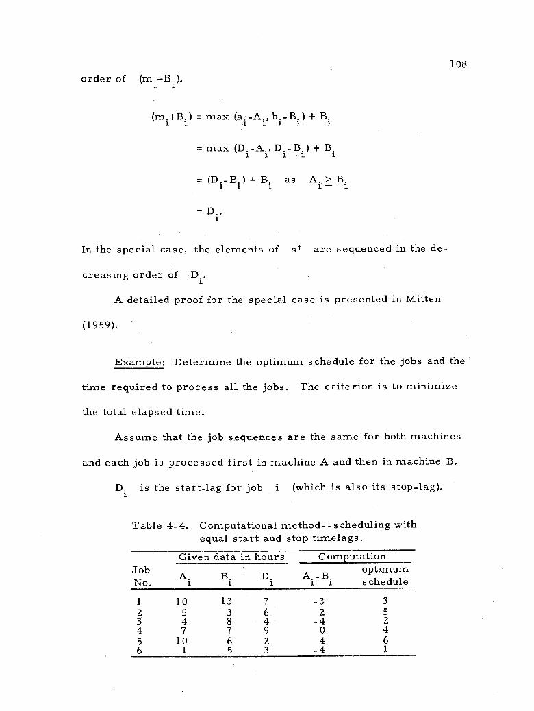
108

order of (m.+B.). 1 1

(m.+B.) = max (a.-A., b.-B.) + B. 1 i 1 1 1 1 1

= max (D.-A., D.-B.) + B. 1 1 1 1 1

= (D.-B.) + B. as A. > B. 1 1 1 1- 1

= D.. 1

In the special case, the elements of s' are sequenced in the de-

creasing order of D..

A detailed proof for the special case is presented in Mitten

(1959).

Example: Determine the optimum schedule for the jobs and the

time required to process all the jobs. The criterion is to minimize

the total elapsed time.

Assume that the job sequences are the same for both machines

and each job is processed first in machine A and then in machine B.

D. is the start -lag for job i (which is also its stop -lag). 1

Table 4 -4. Computational method - -scheduling with equal start and stop timelags.

Given data in hours Computation Job No.

A. 1

B. 1

D. i

A.-B. i i optimum schedule

1 10 13 7 --3 3

2 5 3 6 2 5 3 4 8 4 -4 2 4 7 7 9 0 4 5 10 6 2 4 6 6 1 5 3 -4 1

B

The optimum schedule is 6-3-1-4-2-5.

A I. (1) (4) (2 (5) 4=mmul

10 20 30 40 50


Total elapsed time = 45 hours.

109

Applicability of Start and Stop Lags: Overlapping of production:

In certain instances, sequential operations can be overlapped so that

the same job can be processed by two operations at the same time.

For example, in building a house, painting can start after some in-

terior woodwork has been completed but before all the interior wood-

work is finished. Another example can be found in an engineering pro-

ject, where drafting works can be started anytime after a, weeks

of design work, but that drafting may not be completed before the de-

sign work is completed (b_. = 0). In such situations where opera- ].

tions do overlap this method of scheduling may be found useful.

Delays between two machiens: The transportation time be-

tween two machines and other delays can be incorporated in the values

of start and stop lags. This procedure can also be applied in

I i i 1

i

110

situations of two "bottleneck" machines (highly loaded machines,

and B) of a production line.

After being processed on machine A, the jobs may (or may not)

have been routed through a variety of intermediate (non- bottleneck)

machines before being started in machine B. In such cases,

a. _ (time to complete intermediate operations on job i

+ any initial minimum backlog required)

and b. = (time to complete intermediate operations + any minimum

final backlog required).

It may also be noted that Johnson's rule (1954) is a special case

of the above algorithm in which a. 1

= A. 1

and /or b. = B. for all i. 1 1

3. Generalized Johnson's Rule for Job -Lots

Jackson (1956) has extended Johnson's two stage rule so that it

is now applicable where each job falls in any one of the following four

sets:

Set A: Jobs which require processing by machine I only.

Set B: Jobs which require processing by machine II only.

Set C: Jobs which require processing first by machine I and then by

machine II.

Set D: Jobs which require processing first by machine II and then by

machine I.

A

111

All assumptions stated under Johnson's method hold true except

for the condition of common order in the machines (B -3).

The computational procedure for the extended case is:

Step (1): Group the jobs into four sets, A, B, C and D as given above.

Step (2): Sequence the jobs in the Sbt C according to Johnson's Rule

taking machine I as machine A and machine II as machine B

and denote the schedule as "order Cl."

Step (3): Sequence the jobs in the Set D according to Johnson's Rule

taking machine II as machine A and Machine I as machine B

and let the schedule be known as "order D1."

Step (4): Schedule the jobs of Set C first in machine i as in "order C

Step (5): Order the jobs of Set A next (in any sequence) in machine I.

Step (6): Order the jobs of Set D next in machine I as in "order D1."

Step (7): In machine II, sequence the jobs of Set D first (as in "order

D1 "), then jobs of Set B next (in any sequence) and the jobs

of Set C last (in the sequence previously obtained in "order

Cl"). Now we have scheduled the Sets A, B, C and D in

machines I and II as shown in Figure 4 -7. The proof of this

is identical with Johnson's Rule.

More in- process inventory is required for this model (than of

Johnson's Rule) since the common order of processing is not adhered

to on both of the machines.

from the Gantt chart.

The total elapsed time can be established

'

112

Machine I

Machine II

Á \

Set C

-

Set A

,

Set D

/

e-1 ° ... Set D Set B Set C

ti Figure 4 -7. Scheduling of job lots in two machines (Johnson's

method).

Example: The following 12 jobs are to be scheduled in a print-

ing press so that the time required (hours) to complete all the jobs

is minimized.

Table 4 -5. Job list for a printing press.

Set A B C D

Job No. Al A2 A3 B1

B2 B3 C1 C2 C3 D1

D2 D3

Machine I 5 8 2

Machine II 7

10 7 4 6 13 8

1 3 12 9 12 4 7

For the Set C, the order is

For the Set D, the order is

(C3,

(

C2, C1)

D3, D1)

For the Set A and Set B any random order is allowed. Then for

Set A, let it be (Al, A3, A2) and for Set B, let it be (B3, B1, B2).

4

".. \ ....I ¡ i' _ ...

k

9

-f

--*

113

Machine I

Machine II

Machine I

Machine II

C3 C2 Cl

D2 D3 D

A

D3 D1

C3 C2 C1

D

D B C

&\

10 20 30 40 50 60 70

Figure 4 -8. Gantt chart for the optimum schedule.

The optimal schedule is shown in Figure 4 -8 and the total

elapsed time is 64 hours.

Al A3

B3 B1

A2

B2

D2

../.00111\11M4

1 I 1 1 1 t 1

114

V. THREE STAGES - -SETUP TIME INCLUDED WITH PROCESSING TIME

A. Elapsed Time

The classic three -machine sequencing problem can be stated as

follows:

n jobs are to be scheduled on each of the machines A, B

and C. Each job is first processed in machine A, then in B and next in C. The processing time for each job on each machine is deterministic. The objective function is to minimize the total elapsed time.

To date, no outstanding simple method is available for deter-

mining the optimum schedule for this historic scheduling problem.

Johnson (1954) has presented an algorithm for a restricted situ-

ation of the three -machine sequencing problem.

Giglo and Wagner (1964) have formulated three computational

methods and presented their experimental results based on these

methods.

1. Johnson's Rule (a Restricted Case)

The computational method developed by Johnson (1954) can be

applied to the three- machine problem for obtaining the optimum

schedule if and only if either or both of the following conditions hold:

(i) The smallest processing time for machine A is at least as

great as the largest processing time for machine B.

Let

115

(ii) The smallest processing time for machine C is at least as

great as the largest processing time for machine B.

a. = processing time in machine A for job i.

b. = processing time in machine B for job i.

c. = processing time in machine C for job i.

d. - a. + b. 1 1 l'

e. = b, + c. 1 i. l'

The restriction is that min a. > max b. or min c. > max b.. 1= J 1 = J

Algorithm:

Step (1): Examine the a,'s, b.'s and c,'s for all items and see if 1 1 I

the condition min a. > max b. or min c. > max b, is 1= 3

1= J

satisfied. If satisfied, go to Step (2). If not, the problem is

not solvable by this algorithm.

Step (2): For each item compute d, and e, and list them in two 1 1

vertical columns.

Step (3): Scan all the di 1

and e, values for all items and choose

the smallest one.

Step (4): If it is a d.1 , place the item first. If it is an e,, place

the corresponding item last.

Step (5): Cross off the di and ei values for that item in the list.

Step (6): Go to Step (3). The method is repeated till all the items

116

are crossed out in the list. Ties, if any, may be broken

arbitrarily.

From the Gantt chart, we can determine the total elapsed time.

A detailed proof is presented in Johnson (1954).

Example: A bookbinder has six jobs and the time required (in

hours) to perform the printing, binding and finishing operations for

each job is known. The bookbinder wishes to determine the order in

which the tasks should be processed, in order to minimize the total

time required to turn all the jobs.

Table 5 -1. Job list of a bookbinder.

Job No. Printing time

ha. (rs) Binding time

bi (hrs) Finishing time

ci (hrs )

1 30 80 120 2 120 100 130 3 50 90 140 4 20 60 180 5 90 30 100 6 110 10 170

min ci( =100) > max b.(z--100) we can apply this algorithm.

Table 5 -2. Computational method.

Given data d. e.

Optimum order i a. b. c.

1 30 80 120 110 200 2

2 120 100 130 220 230 6

3 50 90 140 140 230 5

4 20 60 180 80 240 1

5 90 30 100 120 130 3

6 110 10 170 120 180 4

As J

ai

--

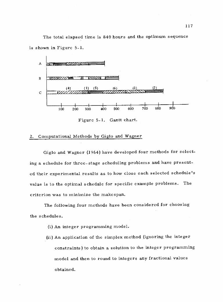
117

The total elapsed time is 840 hours and the optimum sequence

is shown

A

B

in Figure 5 -1.

`l.Ó

n /.11.1\=1111111iIIIIII\\\\\\EI

C

(4) (1) (5) (6) (3)

}

100 200 300 600 700 80} 0 9 0 400 500

Figure 5 -1. Gantt chart.

2. Computational Methods by Giglo and Wagner

Giglo and Wagner (1964) have developed four methods for select-

ing a schedule for three -stage scheduling problems and have present-

ed their experimental results as to how close each selected schedule's

value is to the optimal schedule for specific example problems. The

criterion was to minimize the makespan.

The following four methods have been considered for choosing

the schedules.

(i) An integer programming model.

(ii) An application of the simplex method (ignoring the integer

constraints) to obtain a solution to the integer programming

model and then to round to integers any fractional values

obtained.

111110111%////Ó

I a 4 I I

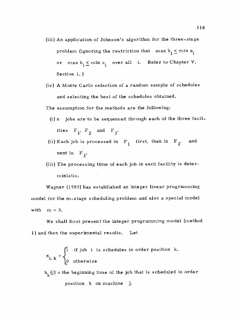
118

(iii) An application of Johnson's algorithm for the three -stage

problem (ignoring the restriction that max b. < min a.

or max b. < min c. over all i. Refer to Chapter V.

Section 1. )

(iv) A Monte Carlo selection of a random sample of schedules

and selecting the best of the schedules obtained.

The assumption for the methods are the following:

(i) n jobs are to be sequenced through each of the three facil-

ities F1, F2 and F3.

(ii) Each job is processed in F1 first, then in F2, and

next in F3.

(iii) The processing time of each job in each facility is deter-

ministic.

Wagner (1959) has established an integer linear programming

model for the m -stage scheduling problem and also a special model

with m = 3.

We shall first present the integer programming model (method

1) and then the experimental results. Let

xi ,k = otherwise

1 if job i is schedules in order position k.

0

bk(j) k(j) = the beginning, time of the job that is scheduled in order

position k on machine j.

1-

119

dk(j) = the time between completion of the job in the order posi-

tion k on machine j to the starting of the same job

in the (j +l) -th machine.

sk(j) = time elapsed on machine j from the completion of job

in order - position k to the starting of job in order -

position (k +l) in the same machine.

ti( j) = processing time of job i in machine j.

All variables are non -negative integers. The job i is said to

be scheduled in order position k on machine j if prior to this job

being placed on machine j, (k -1) jobs have been processed on it.

Each job must be processed in some order -position and there-

fore, we have

x = i i, k for all i (1) /

k =1

As there is some job in each order -position, we have the con-

s tr aint

n

xi, k= 1 for all k.

i=1

(2)

Johnson (1954) has proved that there shall be at least one opti-

mal sequence in the set of schedules which are obtained on the

/

120

presumption that the n -jobs are processed in the same order on all

three machines.

It is also assumed in this algorithm that the n tasks are pro-

cessed in the same order on all the facilities.

To satisfy the assumption (ii), the following set of constraints

are introduced:

b k(j) _ k-11'

n

dk-l) + ti(j-1) ° Xi, k i=1

(for k = 1, 2, 3, . . . , nm 1)

(3)

The following set of restrictions are required to see that only

one job can be processed on the same facility at any given time.

bk (j ) = b k-1) + -(k-1) + f(i)X(k-1) (4)

for k = 1, 2, 3, ... ,

All variables are nonnegative integers (5)

Minimizing the total makespan is equivalent to minimizing the slack

time on machine F3. Therefore, the objective function is

Minimize z =t(1)+ti2)+si3)+s3)+... s(n3)1.

The integer linear programming model for the n -job, m-

machine scheduling problem constructed by Giglo and Wagner (1964)

(k-1)

(n -1).

121

is described in Chapter VI. Section B -3.

Giglo and Wagner (1964) have tested these methods on 100 prob-

lems with n = 6. The following results have been obtained:

(a) The methods presently available for solving the integer pro-

gramming problems do not appear to be efficient. A 6 -job

problem requires a total of 720 permutations ( =6! ). How-

ever, the integer linear programming model was not able to

establish the optimal schedule even in 10, 000 iterations for

some 6 -job problems.

(b) The linear programming rounded solutions averaged about

an 11 percent increase over the optimal processing time.

This method tended to yield sequences that were better than

those that would be obtained by a single permutation drawn

at random.

(c) The heuristic method based on Johnson's Rule was tested on

20 of the 100 cases. The average ratio of optimal value to

the Johnson solution value was found to be 0. 97 and thus gave

excellent results_

(d) The random sampling method did not yield any indication of

whether or not the best obtained solution was actually optimal

and if not, how close was it to the optimal value.

122

VI. M- STAGES- -SETUP TIME INCLUDED WITH PROCESSING TIME

Most problems of scheduling tasks in such multi -stage indus-

trial situations as those usually encountered in a chemical plant, a

machine shop and a ship building yard require an m -stage computa-

tional method. In this chapter, we shall consider the general sched-

uling problem of sequencing n jobs on m- machines (m > 3).

Various approaches and algorithms for minimizing the total tardiness,

make -span, in- process inventory cost or sum of production and stor-

age costs are presented. These algorithms are also used generally

to solve three -stage scheduling problems, since the latter do not yet

seem to have their own simple and elegant computational method.

We observe that these algorithms require a very large number

of computations and involve many computational difficulties. An

n -job m- machine scheduling using a brute force technique involves

the calculation of all (n! r schedules and choosing one that has the

minimum or maximum value as required by the objective function.

Therefore, it may be stated that these computational methods require

less computational effort than the brute force method.

123

A. Tardiness

1. Total Tardiness Over All Jobs

Brooks and White (1965) have developed a model using the pro-

cedure of Griffer and Thompson (1959, 1960) and also the branch and

bound algorithm by Little, et al. (1963) for determining the optimal or

near optimal solutions for n -jobs to be scheduled on m- machines.

The criterion is to minimize the total tardiness (lateness) for all

jobs. It is not required that the technological ordering for each job

must be the same.

We have already discussed tardiness, total tardiness and other

terminology in Chapter II -A.

We shall state the assumptions and discuss some operations of

the computational method first and then present the algorithm for de-

termining the optimum schedule.

Assumptions;

1. The processing times are deterministic.

2. The working times are independent of the order in which

the operations are performed. Transportation and setup

times are included in the processing times.



124

completion. A given job may be processed on only one ma-

chine at any given time.

4. Only one machine per type is allowed in the problem.

A sequence array (S) specifies the technological ordering of

each job on different machines. For instance 2 -3 -1 -4 means that the

job is first processed in machine 3, second in machine 1, third in

machine 2 and fourth in machine 4. The technological order of all

jobs in different machines must be completely specified.

where

on the

s.,

j -th

S =

is the

machine.

s11 s12 s13

s21 s22 s23

sn2 sn3

"' "'

i -th

slm

s2m

s nm

be processed order in which the job will

A facility array (F) states the times required to process each

F

job in different machines.

f12

f22

fn2

...

"'

...

fll

f21

fnl

flm

f2m

fnm

snl "

=

it

125

where f.. is the time to process the i -th job on the j -th ma- 1J

chine (facility). If the k -th job is not processed in the p -th

machine, then fk = O. p

A problem array (P) denotes the minimum time required to

complete each job on different machines with no overlap of operations

for any job (overlap of operations on the facilities is allowed). This

is computed from the F -array and the S- array.

P =

p11

p21

pn 1

P12

p22

pn 2 °"

plm

p2m

pnm

where . . is the minimum time to complete the i -th job on the 1J

j -th machine.

For example, let us consider the following S- and F- arrays.

2 1 4 3

S =

1 2 3 4

7 8 5 9

F =

12

and then,

15 8 29 24 P =

6 10 13 25

"'

6 4 3

126

By observing the position of the numbers in the problem array,

we can find the ordering of the job in the machines. For job 1, the

first smallest number is 8 (in the second column) and so the job is

processed in machine 2 for 8 time units. The second smallest num-

ber is 15 (in the first column) and hence the job is processed second

in machine 1 for 7 ( =15 -8) units of time and so on.

A linear array (also referred to as "work array ") can be re-

garded as a set of m boxes (m being the total number of machines),

indexed by machine -job pairs. The boxes are grouped in blocks sep-

arated by double lines and that each block contains boxes representing

the jobs that are to be processed by that machine. Thus, the j -th

block can be called the j -th machine block because it contains a

box for each job that requires processing by machine j. The linear

array can be drawn as in Figure 6-1.

M1 M2 M3

JI J2 Jn J1 J2 °'° Jn J1 J2 °°° Jn

Figure 6 -1. Linear array.

Jobs in Conflict: When more than one job is scheduled for the

same machine for some common interval of time, the jobs are said

to be in conflict.

127

For example, let us consider the schedule of three jobs on four

facilities.

1

1 2

S = 1 2

2

5 8

F = 2 4

Li 6

r 5 13

P = 2 6

13

3 4

3 4

3 4

7 2

3 5

5 9

20 22

9 14

18 27

Job (i) Due date (di)

2

3

20 25 30

Jobs 1, 2 and 3 are in conflict in facility 1 as job 1 is tentatively

scheduled in F1 for the time interval 0 -5 days, job 2 for 0 -2 days

and job 3 for the time interval 0-7 days.

Resolving a Conflict: If there is a conflict between k jobs in

facility j, then k -lower bounds are determined by resolving on each

one of the k jobs temporarily. Care is taken to see that there is

7

1

128

no overlapping of jobs in the last machine. If there is any overlapping

in the last machine, then the jobs are scheduled in it according to the

first in -first out (FIFO) rule.

The tardiness for each job is computed using the equation:

where

t. = max {(Ci-di), 0}

t. = tardiness for job i i

C. = the completion time for job i

d. = deadline for job i. i

The lower bound is the sum of tardiness over all jobs. The

k -lower bounds are then compared and the one with the least of the

lower bounds is chosen, which corresponds, for example, to resolv-

ing on job r. Hence, we resolve the conflict by deciding on job r,

which is likely to give us a schedule with a minimum total tardiness.

Let us illustrate this in the problem stated above. There is a

conflict between jobs 1, 2 and 3 in F1. Resolving the conflict by

choosing job 1:

P

5 13 20 22

7 11 14 19

12 18 23 32

Lower bound for job 1 is 4 days.

C. t. i x

22 2

19 0

32 2

=

Resolving on job 2:

C. i

t. I

7 15 22 24 31 11

P W 2 6 9 14 14 0

9 15 20 29 29 0


Resolving on job 3:

C t.

12 20 27 29

P = 9 13 16 21

7 13 18 27

1 1

32 12

21 0

30 0

129


The least of the 3 lower bounds is 4 days, and hence, we re-

solve the conflict by choosing J1 in this situation.

The resolution can be represented by a decision tree where the

decisions are represented by nodes and the conflicts by branches.

The decision tree is illustrated in the following example, Figure 6 -2.

Constraints like rush jobs and jobs in processing can also be

introduced. In resolving the conflicts, the job in processing has the

priority over all other members. We assigna lower bound of infinity

to these members. Similarly, a rush job is to be chosen, in case of

a conflict, over all jobs (excepting the job in processing). The lower

_ -

130

bounds for these jobs are set at infinity.

Algorithm:

Step (1 ): Construct a work or linear array and enter the completion

time of the first operation of each job in the linear array.

Set T equal to the smallest of these times.

Step (2): For each machine, check for conflicts between the jobs end-

ing at time T and those ending later than time T.

Step (3): Check the members of the conflict for the constraints (like

rush order, job in processing, etc. ). If there are no con-

straints go to Step (4). If there are any constraints, resolve

the conflicts accordingly. Go to Step (5).

Step (4): Compute the lower bound for each member of the conflict.

Choose the member having the least lower bound and the con-

flict is resolved about this member. Ties, if any, may be

broken arbitrarily.

Step (5): For each T in the work array find the next machine, if

any, to process the job and enter the value (t +f), where

f is the processing time for the new operation, in the array.

Step (6): If T is the largest entry, go to Step (7). If not, find the

value T' in the array that is the next largest to T and

set T = T'. Go to Step (2).

Step (7): Examine the previous conflict level and compare the lower

131

bounds to the obtained solution. If any lower bound is less

than this solution, go to Step (3) to determine the optimal

solution.

The schedule determined already is the near - optimal

solution. On the other hand, if all lower bounds are greater

than or equal to the solution, back up one level and repeat the

step. If all levels are checked, then the optimal solution is

the last solution obtained.

Example: The following 4 jobs, (J1, J2, J3 and J4) are to

be sequenced on 4 machines M1, M2, M3 and M4. For each job

the technological processing order, processing time (hours), deadline

(d.) and constraints are known.

d. Constraints 1

1 2 3 4 45

1 2 work in process Sequence array, S =

1 2 3 4 50 rush order

1 3 4 2 60

10 9 7 15

10 3

Facility array, F =

5 14 16 8

10 12 15 20

- -

132

7 17 26 41

10 13 13 13 Problem array, P t

5 19 35 43

10 42 57 30

Level 1: Conflict is between J1, J2, J3 and J4 in M1. The

conflict is resolved about J2 as it is already in process.

17 27 36 51

10 13 13 13 P

15 29 45 53

20 52 67 40

Level 2: Conflict is between J1, J3 and J4 in M1. The rush

order J3 is chosen.

P

22 32 41 56

10 13 13 13

15 29 45 53

25 57 72 45

Level 3: Conflict is between J1 and J4 in M1. Choosing J1,

=

=

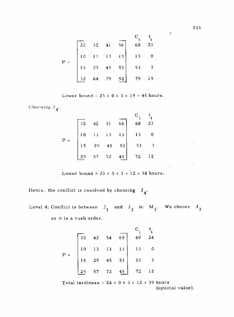
133

P

41

13

45

79

C. t, i ì

68 23

13 0

53 3

79 19

22 32

10 13

15 29

32 64

56

13

53

52

Lower bound = 23 + 0 + 3 + 19 = 45 hours.

Choosing

C, t, i i

32 42 51 66 68 23

10 13 13 13 13 0

P =

15 29 45 53 53 3

25 57 72 45 72 12

Lower bound = 23 + 0 + 3 + 12 = 38 hours.

Hence, the conflict is resolved by choosing

Level 4: Conflict is

as it is a rush

between

order.

J1 and in

C, i

M3. We choose

t. i

32 42 54 69 69 24

10 13 13 13 13 0

P =

15 29 45 53 53 3

25 57 72 45 72 12

Total tardiness = 24 + 0 + 3 + 12 = 39 hours (optimal value).

3 .

J4.

J3 J

Start

denotes level k

134

Figure 6-2. Decision tree for determining the optimal schedule (minimizing the make span).

135

The conflicts, members of the conflict and the decisions are

shown in the linear array (Table 6-1) and in the decision tree (Figure

6 -2).

Table 6 -1. Linear array.

Level Machine 1 Machine 2 Machine 3 Machine 4

J1 J2 J3 J4 J1 J2 J3 J4 J1 J3 J4 J1 J3 J4

1

2

3

4

7c

17c

22c

32

32

10c

10

10

10

10

5c 10c

15c 20c

15 25c

15 25

15 25

42

42

13

13

29

29

57

57

51c c 45c

54 45

72

72 69 53

45

45

The optimum schedule is represented in the Gantt chart, Fig-

ure 6-3.

1

M2

M3

M4

J3 J4 Ji

sv!!/!!/1. 1\\\1!1111111°mllwn111m1umu

11111inunmuiimmmuuu

111I1 Ui111i11111111111111111111

10 20 30 40 50 60 70


J2

- l

8

136

B. Elapsed Time

In this section, we present techniques for establishing the

optimal m -stage schedule(s) when the criterion is to minimize the

total time elapsed from the starting of processing the first job to the

completion of processing the last job.

1. Combinational Analysis

Giffler and Thompson (1959, 1960) are credited for a matrix

method, a linear algorithm and a Monte Carlo technique for open,

dual -open and mixed scheduling problems.

Brooks and White (1965) and Ignall and Schrage (1965) have

each developed algorithms (for open scheduling problems) based on

the branch and bound technique by Little, et al. (1963).

Deduk and Teuton (1964) have established an algorithm for ob-

taining one or more optimal sequences utilizing the combinatorial

analysis.

(a) Matrix Method. The algorithms developed by Giffler and

Thompson (1959, 1960) are applicable for a wide variety of production

scheduling situations. We present the algorithms for obtaining the

optimal schedule when the optimizer is minimizing the total elapsed

time.

For each job, the order in which it is to be processed in

137

different facilities is usually known from the technological point of

view. Then we say that the next relation to follow for the jobs in dif-

ferent machines are prescribed. Sometimes, these "next- follows"

relations for each facility of processing different tasks are known.

The i -th facility sequence F., specifies the order in

which job Ji is processed in successive facilities. The facility

sequence matrix F is an ordered collection of the facility se-

quences.

F =

J 1

y 1 2 3 ... m

1 2 3 ... m

1 2

We note in the above F matrix that job 1 is processed first in

machine 1, then in 2, next in 3 and so on.

The F- matrix will be rectangular only if each job is processed

by the same number of facilities and it will be square only if, in addi-

tion to the above restriction, the number of jobs is the same as the

number of facilities in which any job is processed.

Similarly, the j -th job sequence, J., indicates the suc- J

cessive jobs that are processed by facility, F., The job sequence

matrix J is a collection of the job sequences. The job matrix J,

can be represented as:

J2

J n

J>

F - F2 -.

J = F3-

3 ... n

1 3

1 2 3 ...

Fm--IJ. 2

138

A schedule is said to be feasible if each job and facility have a

finite number of next - follows relations, it satisfies all technological

requirements, at a given time no facility processes more than one

job and also no job is processed_in more than one facility at a given

time.

The facility and job sequence matrices with the idle times in-

serted at the proper places are known as Gantt charts and represented

by G(F) and G(J). In these Gantt charts, the idle time is denoted

by a dash.

The Gantt charts are non -numeric when the actual processing

time for each operation is not taken into account in constructing the

chart, but assumed to be equal to one unit of time (or one "schedule

step ") for each operation. The (i, k) -th entry in G(F) will be the

index j indicating that the job i is processed in facility j in

step k and will be a dash if i is idle in step k. Similarly, the

(j, k) -th entry of G(J) will be the index of the job i indicating

that the facility j is processing job i in step k and will be a

dash if j is idle in step k.

1 2

n

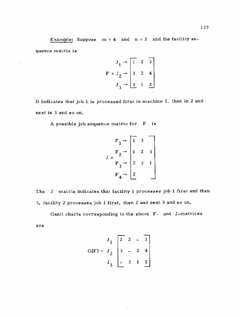
139

Example: Suppose m = 4 and n = 3 and the facility se-

quence matrix is

J1 . 1 2

F J -- 3 2 4

J3-- 3 1 2

It indicates that job 1 is processed first in machine 1, then in 2 and

next in 3 and so on.

A possible job sequence matrix for F is

The J matrix indicates that facility 1 processes. job 1 first and then

3, facility 2 processes job 1 first, then 2 and next 3 and so on.

Gantt charts corresponding to the above F- and J- matrices

are

J1 2 - 1 3

G(F) = J2 3 2 4

J3 3 1 2

3

F 1 3 1

F2 - 1 2 3

F3 - 2 3 1

F 2 4

J

-

-

F G(J) =

2

1 3

1 2 3

2 3 1

_ 2

140

The Gantt charts are numeric when the actual processing times

to perform the operations are taken into account in constructing the

charts. It is assumed that the processing time for each job is an

integer. For instance, if we assume in the example above that oper-

ation (J., F.) J

is G(F) and

requires

G(J):

i +j hours, we obtain the following numer-

J1 1 1 2 2 2 3 3 3 3- G(F) = J2 3 3 3 3 3 2 2 2 2 4 4 4 4 4 4

J3 3 3 3 3 3 3 1 1 1 1 2 2 2 2 2

1 3 3 3 3 1

F2 - 1 1 1 2 2 2 2 3 3 3 3 3

G(J) =

- F3 2 2 2 2 2 3 3 3 3 3 3 1 1 1 1

F 4

2 2 2 2 2 2---

We note that G(F) and G(J) have the same number of col-

umns if they are obtained from the same F and C matrices.

The number of columns in the numeric G(F) or G(J) represents

the length of time required to complete all operations. We require 20

F

F

F

1

3

4

F 1

- -

-

-

-

141

hours to complete the jobs according to the G(F) and G(J).

An active feasible schedule is a feasible schedule such that,

(1) no facility is idle at the time there is an idle job it can process,

and (2) each operation starts as soon as all operations which precede

it directly (it "next-follows" them) are completed. Two schedules are

said to be equivalent if, and only if, one schedule can be obtained

from the other by a sequence of permissible interchanges of opera-

tions with idle times or with other operations. On interchanging the

operations, care should be taken to see that the technological require-

ments are not violated and the total elapsed time remains the same.

For instance, in our previous example, we had:

G(F) = 3 - 2 4

3 1 2

We observe that job 1 and facility 3 are idle in Step 3 and therefore

this is not an active feasible solution. An equivalent schedule for this

is

1 2 3

G(F) = 3 - 2 4

3 1 2

This is an active feasible schedule and also we note that both schedules

1 2 3 ' -

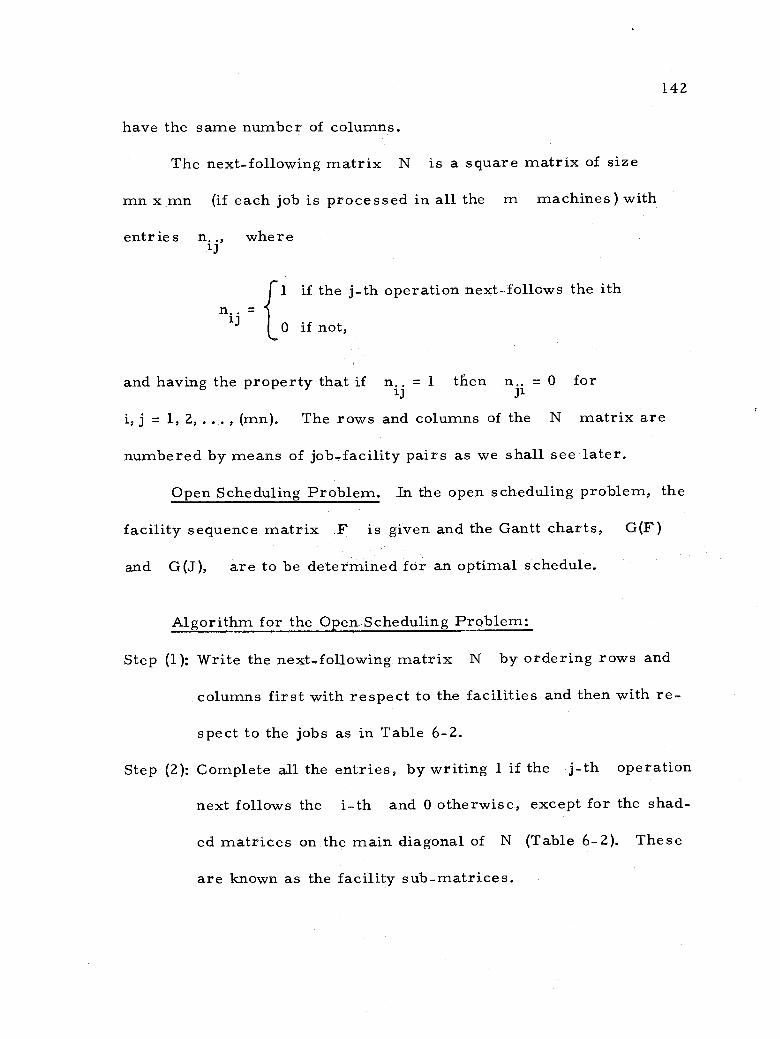
have the same number of columns.

The next - following matrix N is a square matrix of size

mn x mn (if each job is processed in all the m machines) with

entries n.., where 1J

1 if the j -th operation next -follows the ith

0 if not, ,

142

and having the property that if n.. = 1 then n, = O for iJ Ji

1, j = 1, 2, ... , (mn). The rows and columns of the N matrix are

numbered by means of job -facility pairs as we shall see later.

Open Scheduling Problem. In the open scheduling problem, the

facility sequence matrix F is given and the Gantt charts, G(F)

and G(J), are to be determined for an optimal schedule.

Algorithm for the Open Scheduling Problem:

Step (1): Write the next - following matrix N by ordering rows and

columns first with respect to the facilities and then with re-

spect to the jobs as in Table 6 -2.

Step (2): Complete all the entries, by writing 1 if the j -th operation

next follows the i -th and 0 otherwise, except for the shad-

ed matrices on the main diagonal of N (Table 6 -2). These

are known as the facility sub -matrices.

= 13

n.. ¡I

143

Table 6ü2. Matrix N for an open scheduling problem.

Step (3): In each block of columns corresponding to a given facility,

try to find and check one zero column assuming the blank

entries as zeros.

Step (4): Fill in the blanks in the checked columns with zeros.

Step (5): Check the rows corresponding to the checked columns. The

unchecked rows and columns comprise a new reduced matrix.

Step (6): In each block of columns of the reduced matrix (obtained

from the previous matrix) corresponding to a given facility,

check, if possible, one zero column.

Step (7): Enter a 1 in each blank which occurs at the intersection of a

F1 F2

. . .

Fm

J1 J2 . .. Jn J1 J2 . .. Jn J1 J2 . . . Jn

J J2

F 1 ...

Jn J1 J2

F 2 ...

J

/ 4

J1 J2

F m... Jn

/

/

.. /

145

Table 6-3. The initial next - following matrix N.

F 1

F2 F3 F4

J2 0 0 0 0 Fl J3 0 0 1 0

J1 0 0 0

F2 J2 0 0 0

J3 0 0 0

F J1 0 0 1 0 0

3

J2 1 0 0 0 0

J 0 0 0 0 0 1

F 4 J3 0 0 0 0 0 0

0 0 0

0 0 0

0 0 0

1 0 0

0 0 1

0 0

0 0

0

0

Table 6 -4. The reduced N- matrix, No. 1.

F1 F2 F3 F4

J2 1

J2 3 1 J2 J1 J3

J 0 0 0 0 0 0 0 F1 2

I f

J b 0 0 1 0 0 0 0

F3

J1 0 0

J -- 2

0--0 J3 0

J 0 0 1

J2 1 0 0

0 0 0 0 0

I I

I

0-1- 0-0 0 0 0 0 1

I

0 0

0

0

0

J-O-0 F4

I)

0-0-0 1 0 o

0 0 0 0 0

J3 J1 J2 J3 J1 J2 J1 J3

J13

I

F2 0I

0

i

J3 0

0

I

0

J2

6 i

146

Table 6-5. The reduced N- matrix, No. 2.

F2 F3 F4

J3

J1 0 0 0 ¡ 0 0 0

F2 J20 (hO 0 I 0-1- 0-0- 1 1 I I 1 J3--0-0 0-0-F-0-

J -0- 0-1 0 0 0 0 0 F3

J2 1

1 ó 0 ó b g 0

s V I

F4 J1

O 0 j 0 ¡

0

0 J3 0 0

Oi I


F1

_ J

F2

J_

F3 _ J

F4

J

J2 0 0 I

0 0 (0

0 I0

J3 0 0 1 0-- 0- 0- 0

1 I 1

J O 0- 0 0 0 0 1

F2 JZ 0 b 1

J 0- 0

(

I

O

1

1 I 1 I

I 0I 0 I0

I 1 1

I I 1

1 0-0 bb I I I

J - 0- 0 1I-0 - 0-4 I 0 -0 F3

J2-1 I I- I 0-0- 0

I E I I I T)I

¡ I 4 J3-0 0 0 0- 0- 0

F1

F1

J2 J3 J1 J2 J3 J1 J2 J1 J3

J2 0 0 0 0 (!1 0 Ó 0

Ó 0 0 ].--1-0-() 0

1 i 1 1 i

0

0

o

il ¡3 I1

F

I

J 0 0 Q 0-1 I0- 0 -

[ I 1 r t 1 + I

1- I I I

i I

i

147


F1 F2

J

1 I

F1 0 g {-O-Ì-{ - {

J -I-0- -0 1 0-0-0 0 3

F

I

J -0--0 Ó i j- 0 I

1 0 F J -Ó - Ó-01-1 1 - Ó Ó-

2 2 I I

Q

J -0 0-1 0-Ó 0 0-1- 3

J2-1 0-0-0-0-0-0- F J1 I J- i- 0 1 0--],-

4 J3 0 0-0-

Table 6-8. The N- matrix for the optimal schedule.

F1 F2 F3 F4

2 J3 J1 J2 J3 J1 J2 1 J3

J2 0 0 0 0 0 0 0 0 0

1 J3 1 0 0 0 1 0 0 0 0

J1 0 0 0 0 0 0 0 0 0

F2 J2 0 0 0 0 1 0 1 0 0

J3 0 0 1 0 0 0 0 0 1

I, J1 0 0 1 0 0 0 1 0 0

3 J2 1 0 0 0 0 0 0 0 0

J1 0 0 0 0 0 1 0 0 1

4 J3 0 0 0 0 0 0 0 0 0

F4

J2 J3 J1 J3 J1 J2 J1 J3

I I i T Í I I i- - 0 -Q 0 -

I I 1 F L __ F J1-0-7_i_?_ i-

3

I I I 1

Ì

0 0 0 0 a i i I t

F

I

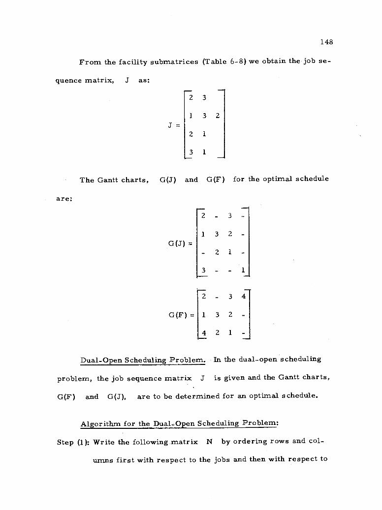
148

From the facility submatrices (Table 6 -8) we obtain the job se-

quence matrix, J as:

2 3

1 3 2

2

1

The Gantt charts, G(J) and G(F) for the optimal schedule

are:

2 - 3 -

1 3 2

G(J) _ -

3

2

as

1

3 4

G(F) _ 3 2 -

4 2 1

Dual -Open Scheduling Problem. In the dual -open scheduling

problem, the job sequence matrix J is given and the Gantt charts,

G(F) and G(J), are to be determined for an optimal schedule.

Algorithm for the Dual -Open Scheduling Problem:

Step (1): Write the following matrix N by ordering rows and col-

umns first with respect to the jobs and then with respect to

J =

1

3

- 1

-

1

2

the facilities as in Table 6 -9.

Table 6 -9. The matrix N for a dual -open scheduling problem.

J1

F1 F2 ... Fm

J2

F1 F2... Fm

Jn

F F2 .. Fm

F1

J1 F2

Fm F1

J2 F2

Fm

J n

F1

F2

Fm

149

Step (2): Complete all the entries, by writing 1 if the j -th operation

next follows the i -th and 0 otherwise, but the shaded

matrices on the main diagonal of N (Table 6 -9). These

shaded matrices are known as the job sub -matrices.

For Step (3) and so on, refer to the algorithm for open sched-

uling problem. The words "Job" and "facility" in the description of

that algorithm are to be interchanged.

/

/'

Z.

Vf4j

...

lii ...

150

From the job sub -matrices, we can determine the facility ma-

trix F.

We shall illustrate the algorithm by a simple numerical ex-

ample.

Example:

J _

e 2 3

1 3 2

3 1

The reduced matrices are shown in Tables 6 -11 to 6 -14. From

the job sub -matrices of the N- matrix (Table 6 -15), we determine the

F matrix.

F =

3 2 4

3 1 2

4 2 1

The Gantt charts for the non -numerical dual -open scheduling

problem are:

T23 - 1 3 2

G(J) =

1 2 -

3 - 1

-

1 2

-

151

Table 6 -10. The initial next -following matrix N.

J1 J2 J3

F2 F3 F4 F1 F2 F3 F1 F2 F4

J1

F2

F3

F4

0

0

0

0

0

0

0

0

0

0

0

0

0

0

0

0

0

1

F1 0 0 0 0 0 0

F2 0 0 0 0 1 0

F3 0 1 0 0 0 0

F1 0 0 0 1 0 0

J3 F2 1 0 0 0 0 0

F4 0 0 0 0 0 0

Table 6 -11. The reduced N matrix, No. 1.

Jl J2 J3 F2 F3 F4 F1

2 F3 F1 F2 F4

F 0 0 I Í

J1 F3 0 0

0 0 0 0 I

0 0 0 0

F4 0- 0-0 0-0-1 I I

F1 0 0 0I 0 I0

0 0

J2 F2 0-0- 0 0 0 1 0 I

F3 0 1 I

0 0 0

1 I I

F -- 1-0-0 - 1 0 0 0

J3 1 0 0 0 f

0 3 2

I I I

F4 0 0 0 0 0 0 0

J2

0

I

152


F2 J F

F4

J1 J2 J3 F2 F3 F 4 F F F F F F 1 1 2 4

0 0 O O b 0

Ó

I

0 0 0 0 j 1

F1 0----0-0 i 0 Q ¡ O

JZ F2-0 0 I I-0 0

I10-1-0

' b 0 b F3 0 1 b 0

I

F--0---0-0-----1-0-0 I -0 b J F ----0 0

F4 0 0 0 0 0 0

1 1 1


J1 J2 J3

IJ ( 0- 0--i -

I { I

0

l

(!)

F3 F4

F -0 4- J1 F3

2

0 y

Ó

F 4

F 0--0 0

J2 F2 0 0-0 F 0-1 F1 0-0- i

F1 F F

J F 1 0 ¡ F4- 6-0-0

1-0-0 I

1 0

CI ? 1--0 I- i I 0-0 0 0--0-9

0

1 3

a I

I

F2

3

i 0-

FI2 FI4

?bd )

0 I I--i 1

P 0 0-0-

t.

153


J1 J2 J3

2 F3 4 F1 F2 F3 FI 1 F2 F4

F2 0 I-0 0-0-0 0-0-v l i I b J1 F3 0 0 0 --0 ° 0

F 1 0- 0 Ó--0 0- 0-1- I I I I I I I E I

F 1 ?___0_O --? 0

I ( -0I J 0-0- 1- - -1 0

2 2 i

QI

F7,---0---1 0 0 0- Ó- 0 Ó I

I { I I f I

0 F1 ( 0 I ? 7 I 1 ?

J3 F2 (

(- i-0 I 0

F4 4

-0-0 0-( --- 0 -0 0

I Fli I

Table 6 -15. The next -following matrix for the optimal schedule.

J1 J2 J3 F2 F3 F4 F1 F2 F3 F1 F2 F4

F2 0 1 0 0 0 0 0 0 0

J1 F3 0 0 0 0 0 0 0 0 0

F4 1 0 0 0 0 0 0 0 1

F1 0 0 0 0 0 1 0 0 0

J2 F2 0 0 0 1 0 0 0 1 0

F3 0 1 0 0 0 0 0 0 0

F1 0 0 0 1 0 0 0 1 0

J3 F2 1 0 0 0 0 0 0 0 1

F4 0 0 0 0 0 0 0 0 0

I

F I

IQ

154

3 2 4 -

G(F) = 3 1 2

4 - 2

The optimum length is 4 steps (4 columns).

Mixed Scheduling Problem. In the mixed scheduling problem,

a part of the F sequence matrix and a part of the J sequence

matrix are given and the Gantt charts, G(F) and G(J), are to be

determined for an optimal schedule.

In establishing an optimal schedule for a mixed scheduling

problem, we can either use the algorithm for the open scheduling or

that for the dual -open scheduling problem. In both cases, the prob-

lem is partly solved and the remaining entries of the N matrix can

be filled in by systematically going through all ways of filling. This

is likely to result in different schedules with different completion

times. The schedule with the smallest step (elapsed time) is chosen

as the optimum schedule.

(b) Linear and Monte Carlo Algorithms. Giffler and Thompson

(1959, 1960) have developed algorithms using the linear array by which

one can generate and evaluate all active schedules and choose the op-

timal schedule(s) directly from this set. When this is not computa-

tionally practical, one can obtain a schedule by a random sampling or

Monte Carlo approach, which can be shown to be optimum with a given

1

155

probability. The probability can be made to approach unity as close

as desired by increasing the size of the sample. The criterion is to

minimize the total makespan.

These computational methods are applicable to the open sched-

uling, dual -open scheduling and mixed scheduling problems and for

the numerical and non -numerical cases. We have described these

problems in Chapter VI, Section B -1(a).

A linear array can be regarded as a set of boxes, indexed by

facility -job pairs (for an open scheduling problem - -as shown in Table

6 -16) or by job- facility pairs (for a dual -open scheduling problem- -

as shown in Table 6 -17). These boxes are grouped in blocks (sepa-

rated by double lines) and each block contains boxes representing the

operations to be performed by a single facility (or a single job). In

each box we shall enter numbers indicating the time at which the oper-

ation is to be performed (for a non -numerical case). In a numerical

scheduling problem, this will represent the time at which the corres-

ponding operation is completed.

If two or more jobs (facilities) are assigned to a facility (job),

then we say that there exists a conflict. By the "resolution of a con-

flict" we mean a selection of the order in which the conflicting mem-

bers (jobs or facilities) shall be processed.

156

Linear Algorithm for the Open Scheduling Problem:

Step (1): Construct a linear array indexing the columns by facility -job

pairs, as shown in Table 6 -16.

Step (2): Enter the completion times of the first operations to produce

each job as given by the facility sequence matrix F.

Step (3): Set T equal to the smallest completion time so entered.

Step (4): In each facility block, check for conflicts for those operations

finishing at T and those completing at later times.

Step (5): In a facility block in which there are c(> 1) operations in

the conflict set, assign one of the operations first and the re-

maining (c -1) operations following it (c ! permutations

are possible) compute the completion times of these opera-

tions. Place them in the corresponding box. Leave un-

changed the completion times of the jobs that are not in con-

flict.

Step (6): From the F- matrix, find, if any, the next operations to be

performed on each job and enter the sum of the completion

times of the previous operation and the new operation time

in the corresponding box of the next operation. Then go to

Step (4).

If all operations are completed and there are no conflicts, these

are the set of active schedules possible for the open scheduling prob-

lem. By examining the total elapsed times of all the schedules, we

157

can determine the optimum schedule.

The Dewey- decimal type notation, as shown in Figure 6 -4, indi-

cates clearly the connection and origin of repeated arrays and the

total elapsed times for the completed schedules.

Example: Open - scheduling problem. Three jobs are to be

scheduled on 4 machines so that the makespan is minimized. The F-

matrix is as follows for the non -numerical case:

F =

2 3 4

3 2

4 2 1

The linear array for this can be represented as in Table 6 -16

and the Dewey -decimal type notation for branching is shown in Figure

6 -4.

Table 6 -16. The linear array for the open scheduling problem.

Schedule D -d F1 F2 F3 F4 Elapsed No. notation J2 J3 J1 J2 J3 J1 J2 J1 J3 steps

1 1 1 2 2 2 1 x 1 11 1 3 1 4 2 2 3 3 1 4* 2 12 1 3 1 3 2 3 2 4 1 4*

x Denotes incomplete schedules. * Denotes optimum schedules.

1

158

12

(4)

Figure 6-4. Resolving conflicts with Dewey -decimal type notation.

In Table 6 -16, we note that we have obtained two active sched-

ules with Steps 4 and hence both of them are the optimal schedules.

The algorithm for the dual -open problem can be obtained from

the above algorithm for open scheduling problem by indexing the lin-

ear array by job - facility pairs (as in Table 6 -17) and interchanging

the words "job" and "facility" in the statement of the algorithm.

Example: (dual -open scheduling problem -- non -numerical case)

The production control department of a forging company wishes to

schedule the following three jobs on the four machines so that the

total elapsed time is minimized.

J =

11

(4)

2 3

1 3 2

1 2

3 1

159

Table 6 -17. Computational method for the dual -open (non -numerical) scheduling problem.

Schedule No.

D -d notation

J J2 Elapsed steps F2 F3 F4 F1 F2 F3 F1 F2 F4

1 1 1 1 1 x 11 1 2 2 1 3 2 2 1 x 12 2 1 2 1 2 2 3 1 x

111 1 2 2 1 3 2 3 1 x 112 1 2 2 1 3 3 2 1 x

1 121 2 1 3 1 4 2 2 3 1 4* 2 122 3 1 2 1 5 2 2 4 1 5

3 1111 1 2 3 1 4 3 2 3 1 4* 4 1112 1 3 2 1 4 3 2 3 1 4*

1121 1 2 3 1 3 3 3 2 1 x 1122 1 3 2 1 3 3 3 2 1 x

5 11211 1 2 3 1 3 4 3 2 1 4* 6 11212 1 2 3 1 4 3 3 2 1 4* 7 11221 1 3 2 1 3 4 3 2 1 4* 8 11222 1 3 2 1 4 3 3 2 1 4*

x Denotes incomplete schedules. * Denotes optimal schedules.

The computation is shown in Table 6 -17 and in Figure 6-5. We

obtain eight active schedules of which seven are optimal schedules

with their total duration of four schedule steps.

In solving the mixed scheduling problems, either the algorithm

for open scheduling problems or that for dual -open problems can be

used. Part of the linear array boxes are filled since parts of F

and J matrices are already known. In filling the remainder of the

boxes, different active schedules may result. The one with the short-

est possible schedule is the optimum schedule.

1 J3

160

o 1111 1112 11211 11212 11221 11222 121

(4) (4) (4) (4) (4) (4) (4)

Figure 6 -5. Resolving conflicts for the dual -open scheduling problem.

122

(5)

2

22

o

161

Monte Carlo Algorithm: In the linear algorithm, the conflicts

are resolved in all possible ways and the resulting schedules are com-

puted. This may require an excessive amount of computation for a

large scale problem. But, in the Monte Carlo approach, the resolu-

tions for conflicts are chosen at random and the elapsed times for

these schedules are then computed. The one with the least amount of

makespan is chosen to be the best schedule.

(c) Application of Branch and Bound Technique.

Algorithm by Brooks and White. Brooks and White (1965) have

developed an algorithm for determining the optimal or near optimal

schedule for the m -stage job scheduling problem. This method is

claimed to be based on the linear algorithm and Monte Carlo. technique

(Chapter IV. B-1-(b)) by Giffler and Thompson (1959, 1960) and also

on the branch and bound algorithm (Chapter 111. 1) by Little, et al.

(1963).

Before studying the algorithm, let us summarize the assump-

tions required and some remarks concerning the method.

Assumptions:

1. The processing time for each job is deterministic and is an

integer quantity. By suitably selecting the time scale, the

operation times can be expressed as integer values. Setup

times are included with the processing times.

162

2. The processing time is independent of the order in which

the jobs are scheduled on the machines.

3. Each job has a technological ordering and it is known com-

pletely. All jobs need not have the same ordering.



completion. A given job may be processed on only one

machine at any given time.

5. Only one machine per type is available for processing.

Conflict Between Jobs: We start processing a job i on ma-

chine j after the previously assigned job is completed on the

machine j. On the contrary, if a job is assigned to start in a ma-

chine before the last started operation has been performed to comple-

tion, we say that there is a conflict between the jobs in that machine.

The problem is specified by using sequence, facility, problem and lin-

ear arrays as previously discussed in Chapter VI, Section A.

Let us illustrate this situation by a simple numerical example.

Sequence array, S =

1 2 3 4

1 2 3 4

1 2 3 4

163

5 7 2 9

Facility array, F (hours)

3 4 7 1

1 5 4 3

and

5 12 14 23

the problem array, P 3 7 14 15 (hours)

1 6 10 13

We note that job 1 is processed in machine 1 for the first 5

hours, job 2 in 1 for the first 3 hours and job 3 in 1 for the first hour.

We say that jobs 1, 2 and 3 are in conflict for processing in machine

Resolving a Conflict: If there is a conflict between k jobs in

machine j then resolving the conflict tentatively about each of the

k jobs (k sublevels) is considered in turn and the total elapsed time

is computed. In calculating the makespan, the conflicts in the inter-

mediate machines are not considered. Only in the last machine, care

is taken to see that there is no conflict between jobs, and jobs are

processed according to their arrival time is the last machine (first

in -first out).

It is to be noted that a job i has to be waiting for being pro-

cessed in the last machine j, if the machine j is still processing

a job that was started earlier. On the otherhand, the machine j

=

=

1.

164

will be idle, if the job i is still being processed in the previous

machine.

In this way, the minimum time required to complete all jobs on

that machine without overlap can be calculated. The lower bound is

the greatest of these times taken over all machines. For each of the

k- sublevels, the lower bound is computed and the least of the k -lower

bounds is chosen (let this be the lower bound for job s). For this

situation (level), we say that the conflict has been resolved by selec-

ting job s.

We shall show this operation for the conflicting situation of the

numerical example. Resolving the conflict by choosing J1,

P =

12 14 23

8 12 19 20

6 11 15 18

=23

(26+1) = 27

(23+3) = 26

The three jobs enter the last machine in the order 1 -3 -2. Job 1 is

processed till the 23rd hour, then job 3 is processed till the 26th

hour and then job 2 is processed during the 27th hour. The lower

bound for this sublevel is 27 hours. Resolving by choosing J2,

P =

8 15 17 26 = 26

3 7 14 15 ---- 16+1=17

4 9 13 16 = 16

5

--

The lower bound is 26 hours.

Applying J3 in machine 1 first,

6 13 15 24

P = 4 8 15 16

taking J2 last; taking J1 last 15 +9 =24; 16 +9 =25

24 +1 =25; 15 +1 =16

1 6 10 13 = 13.

165

The lower bound is 25 hours.

We can not sequence the second job (J1 or J2) on the last

machine right after job 3 (completed on. the 13th hour) as the process-

ing of either job 1 or 2 is not completed till the 15th hour in machine 3.

The least of the three lower bounds is 25 and hence, we resolve

the conflict about machine 1 by selecting job 3.

This situation can be represented by a decision tree with three

branches generating from the node, where the node represents a de-

cision and the branches represent the members of the conflict as

shown in Figure 6 -6.

tI\ Figure 6-6. Resolving the conflict.

166

If all jobs are considered equal in importance, we resolve the

conflicts by choosing a job which has the least lower bound. Suppose,

if there is a rush job, then conflicts can be resolved by choosing this

job and assigning infinity as the lower bounds for the remaining mem-

bers of the conflict.

Algorithm:

Step (1): Construct a linear array (work array) and enter the comple-

tion time of the first operation of each job in this array.

Set t equal to the smallest of these times.

Step (2): For each machine check for conflicts between the jobs ending

at time t and those ending later than time t.

Step (3): Check the members of the conflict for constraints (like rush

order). If there are no constraints go. to Step (4).

If there are any constraints, resolve the conflicts ac-

cordingly. Go to Step (5).

Step (4): Compute the lower bound for each member of the conflict.

Choose the member having the least lower bound and the con-

flict is resolved by selecting this member.

Ties, if any, may be broken arbitrarily. If a lower

bound is greater than or equal to the best solution found, set

this lower bound to infinity.

Step (5): For each t in the work array find the next machine, if

167

any, to process the job and enter the value (t + f), where

f is the processing time for the new operation, in the array.

Step (6): If t is the largest entry go to Step (7). If not, find the val-

ue tt in the array that is next larger than t and set

t = ti. Go to Step (2).

Step (7): Examine the previous conflict level and compare the lower

bounds to the obtained solution. If any lower bound is less

than the solution, go to Step (3) to determine the optimal

solution. The schedule determined already is the near -

optimal solution.

On the other hand, if all the lower bounds are greater

than or equal to the solution, back up one level and repeat the

step. If all levels are checked, then the optimal solution is

the last solution found.

Example: The following data pertaining to the production of

three jobs in four facilities are available to the planning department

of a textile mill. The manager is facing the problem of determining

the order in which the jobs are to be sequenced so that the total

elapsed time is minimized.

Sequence array:

S

1 2 3 4

2 3 4

= 1 2 3 4

1

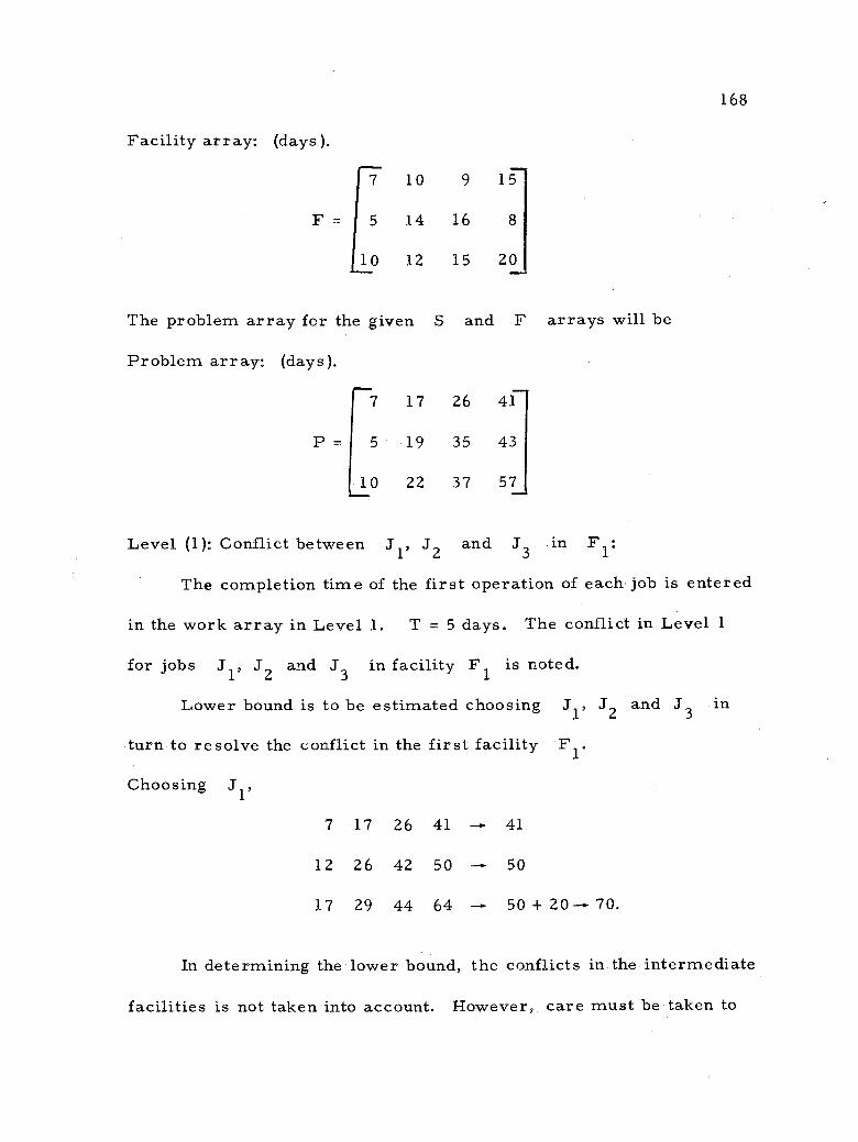
168

Facility array: (days).

7 10 9 15

F I 5 14 16 8

10 12 15 20

The problem array for the given S and F arrays will be

Problem array: (days).

7 17 26 41

P = 5 19 35 43

10 22 37 57

Level (1): Conflict between J1, J2 and J3 in F1:

The completion time of the first operation of each job is entered

in the work array in Level 1. T = 5 days. The conflict in Level 1

for jobs J1, J2 and J3 in facility F1 is noted.

Lower bound is to be estimated choosing J1, J2 and J3 in

turn to resolve the conflict in the first facility F1.

Choosing J, ,

7

12

17

17

26

29

26

42

44

41

50

64

- - -

41

50

50 + 20-.- 70.

In determining the lower bound, the conflicts in the intermediate

facilities is not taken into account. However, care must be taken to

=

-

169

see that in the last facility the jobs are processed in the order of their

arrivals to that stage and the processing is started when the facility

is ready and the job is available.

Though J3 was available on the 45th day, the processing in

F4 could not be started sooner than the 51st day as F4 was occu-

pied by J2 till then.

Choosing J2,

Choosing J3,

12 22 31 46 46

5 19 35 43 (46 +8) -- 54

15 27 42 62 (54 +20) 74. -

17 27 36 51 - 51

15 29 45 53 - 71 + 8 - 79

10 22 37 57 - 51 + 20 - 71

If the conflict is resolved on J1, then at least 70 days will be

required to complete processing all jobs. Hence the lower bound is

70 days for selecting J1.

Similarly by resolving on J2, we get a lower bound of 74

days and on J3, lower bound is 71. Thus, the conflict is resolved

on J1 which has the least lower bound. For each conflict level re-

fer to the linear array (Table 6 -18) and to the decision tree, Figure

6 -7.

--

--

-

Level (2): Conflict between

Choosing J2,

Choosing J3,

7 17

12 26

22 34

7 17

12 36

L17 29

170

J2

26

42

and

41

50

J3

- -

in F1.

41

50

49 69 50 + 20-.- 70.

26 41 -4 41

52 60 -- (64+8)- 72

44 64 64.

Least lower bound is 70.

Conflict is resolved by selecting J2.

Level (3): Conflict between J1, J2 and J3 in F2.

Choosing J1,

17 26 41 41

31 47 55 55

34 49 69 (55+20) 75.

(Since J3 is processed in F1 till the 22nd day, we have sequenced

J3 in F2 from the 23rd day. )

Choosing J2,

36 45 60 - 50 + 15 -- 65

26 42 50 - 50

38 53 73 - 65 + 20 85.

--

-0.

- -- -

Choosing J3,

44 53 68 - 69 + 15 - 84

48 64 72 - 84 + 8 -92 34 49 69 ---



Level (4): Conflict between J2 and J3 in F2.

Choosing J2,

Choosing J3,

17 26 41 -- 41

31 47 55 -- 55

43 58 78 -- 78

69.

17 26 41 41

48 64 72 (69+8) -- 77

171

34 49 69 69



Level (5): Conflict between J2 and J3 in F3. (There is no conflict

for J1 in F3. )

Choosing J2,

26 41 41

64 72 72

79 99 99

- -

- --

-

172

Choosing

26 41 - 41

65 73 -i (69 +8) -- 77

49 69 69.



Level (6): Conflict between J2 and J3 in F4.

Choosing J2,

26 41 -- 41

65 73 73

49 93 - 93.

Choosing J3,

26 41 41

65 77 -- 77

49 69 - 69.



As per conflict level No. 6, we have obtained a schedule with a

total elapsed time of 77 days. Comparing this time to the previous

conflict levels, we note that the levels No. 2 (72 days) and No. 1 (74

and 71 days about J2 and J3 respectively) have less elapsed

time than this. From these three nodes, schedules are to be devel-

oped and their elapsed times are to be compared with that of node

J3,

-

-

173

No. 6. The least among these is the optimum schedule. The near -

optimum schedule is that corresponding to conflict level No. 6 (total

elapsed time is 77 days).

Schedules are computed from level 2 for J3 and also from

level 1 for J3 and the results are tabulated in the work array

(Table 6-18) and are also drawn in the decision tree (Figure 6 -7).

Table 6 -18. Linear array.

Level F1 F2 F

3 F4

E. T. 31 J2 J3 J1 J2 J3 J1 J2 J3 J1 J2 J3

1

2

'C7.5 5c 10c

7 g 17c 17

3 7 12 22 17c 26c 34c

4 7 12 22 17 31c 34c 26 41

5 7 12 22 17 48 34 26 64c 49c 41

6 7 12 22 17 48 34 26 65 49 41 73c 69

Soln. 7 12 22 17 48 34 26 65 49 41 77 69 77

1 7c 5c 10c

1.1 17c 15c 10 22

Soln. 17 22 10 22 > 80

2.1 7 22 17 17 36c 29c

2.2 7 22 17 17 43 29 26 59

2.3 7 22 17 17 43 29 26 60. 44 41 68c 64c

Soln. 7 22 17 17 43 29 26 60 44 41 72 64 72

c Conflict.

OConflict resolved on that job.

E.T. Elapsed time.

.

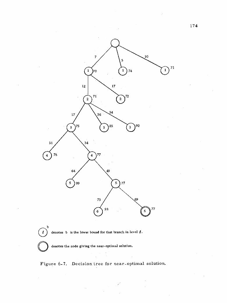
Ob

Q denotes b is the lower bound for that branch in level I.

denotes the node giving the near -optimal solution.

Figure 6 -7. Decision tree for near - optimal solution.

71

174

o

ob Odenotes b is the lower bound for that branch in level Q .

optimum solution.

Figure 6 -8. Decision tree for optimum solution.

175

0

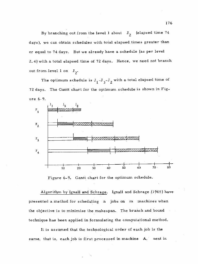
176

By branching out from the level 1 about J2 (elapsed time 74

days), we can obtain schedules with total elapsed times greater than

or equal to 74 days. But we already have a schedule (as per level

2. 4) with a total elapsed time of 72 days. Hence, we need not branch

out from level 1 on J2.

The optimum schedule is J1 -J3 -J2 with a total elapsed time of

72 days.

ure 6-9.

F 1

F2

F3

F 4

The Gantt chart for the optimum schedule is shown in Fig-

J1 J3 12

//,\O\\\

// . N \\ \\\\\\\N

10 20 30 40 SÓ 60 70 80


Algorithm by Ignall and Schrage. Ignall and_Schrage (1965) have

presented a method for scheduling n jobs on m machines when

the objective is to minimize the makespan. The branch and bound

technique has been applied in formulating the computational method.

It is assumed that the technological order of each job is the

same, that is, each job is first processed in machine A, next in

O///1Aw\\'.

/////////.

177

B, then in C, and so on.

We shall now explain the computational method by scheduling

jobs on machines A-B ®C, and then state the algorithm. Let

Sr = a schedule inwhich a subgroup of r jobs have been sequenced.

Sr = the subgroup of (n -r) jobs that have not be scheduled

in Sr. r ao = processing time of job i in machine A.

b. = processing time of job i in machine B.

c, processing time of job i in machine C.

Ta(Sr) = the time at which machine A completes the last of the r jobs

in the sequence Sr. r

Tb(Sr) = the time at which machine B completes the last of the r jobs

in the sequence Sr. r

T (S r ) = the time at which machine C completes the last of the r jobs

in the sequence Sr.

The lower bound of make span for schedules that branch out

from sequence Sr is

Ta(Sr) +

L. B. (Sr) = max Tb(Sr) +

a + min S (bi+ci)

S r r

b. + min- S

ci,

r r

T (S ) + c, c r

5 i

' r

=

c

r

r

z

178

In the corresponding decision tree, the nodes indicate the order of

jobs that have been sequenced so far and the lower bounds are written

next to the nodes.

Dominated nodes: If two séquences, say S' and S ", con-

tain the same jobs and Tb(S') < Tb(S i ), Tc(S') < Tc(S") then we

say that schedule S' dominates S ". We also note that r r

L. B. (S') < L. B. (S ") and also T a (S'r ) = T

a r (S" ). Then, in any - schedule containing S" r at the beginning would not be hurt by replac-

ing S" with S' . We may, therefore, discard the dominated node r r

S" even if its lower bound is less than that of the optimal solution. r

For instance, suppose we have the following two nodes:

Sequence L. B.

2 1 3 15

3 1 2 15

17 16

12 15

The sequence 2 -1 -3 can be ignored in further computations as it is

dominated by the schedule 3-1-2.

Algorithm:

Step (1): Consider that each of jobs 1, 2, ... , n is scheduled, in

turn, in the first order position. Compute their lower bounds

and enter them in the computational list.

Step (2): Choose the schedule with the least lower bound and schedule,

y r r-r r r

Tb Tc

179

in turn, the remaining (n -1) jobs to the second order posi-

tion and determine their lower bounds.

Enter the values of the sequences (nodes) according to

the increasing values of lower bounds. Check for dominance.

Step (3): Choose the schedule with the least lower bound and for its

next order position, calculate the lower bounds for the re-

maining jobs. Check for domiance. The same procedure is

continued till the n -th order position is completed.

Determine the least lower bound of schedules with n-

jobs. Compare this value with the other lower bound values

at previous levels. If there is any node with less value than

this, branch out from that node.

If the lower bounds of other nodes are greater than or

equal to the one we have obtained, this is the optimal solu-

tion.

Example:

Table 6 -19. Job -list for a machine shop.

Jobs Machines

A B C

1 10 5 2

2 3 7 4 3 4 5 8

4 6 2 9

The machine shop foreman wishes to sequence the jobs on three

machines, A, B and C,

mized.

Node 1: 10 + 13 + min (11, 13, 11),

L. B. = max 15+ 14 + min (4, 8, 9),

17 + 21

180

so that the total elapsed time is mini-

Node 2:

= 38

14

3+20+min(13,11,7),

L. B. = max 10 + 12 + min (8, 9, 2),

+ 19

Node 3:

= 33

4 + 19 + min (11, 7, 11),

L. B. = max 9 + 14 + min (9, 2, 4),

17 + 15

= 32

Node 4: .- 6 + 17 + min (7, 11, 13),

L. B. = max 8 + 17 + min (2, 4, 8),

17 + 14

31

We note that node 4 has the least lower bound. Hence, we branch out

from node 41.

=

111111111

Node 42:

Node 43:

L. B. = max

= 31

9 + 14 + min (13, 7),

16 + 10 + min (8, 2),

21 + 10

10 + 13 + min (7, 11),

L. B. = max 15+ 12 + min (2, 4),

25 + 6

= 31.

181

Nodes 42 and 43 have the least lower bound. We choose 43 and

branch out from this. On computing in a similar way, we obtain the

decision tree (Figure 6 -11) and the computational list (Table- .6 -20).

The optimal sequence is shown in Figure 6 -10.

Machine A

Machine B

Machine C

(4) (3) (2) (1) 1IIIIIIIIIIIIIIIIII111% '1101W\\1\\

20 30 40


I

//////// \\\\A

1

..

182

Figure 6 -11. Decision tree.

38 33 32 31

37 31 31

43 31

optimal value)

183

Table 6-20. Computational list.

No. Node Lower bound Tb(Sr) Tc(Sr)

1 0 -- 2 1 38 15 17 3 2 33 10 14 4 3 32 9 17 5 4 31 8 17 6 41 37 21 23 7 42 31 16 21 8 43 31 15 25 9 431 43 25 27

10 432 31 22 29 optimum solution

This method can be extended for scheduling n jobs on m

machines. In general, a minimum of 2

n(n +1) nodes in the deci-

sion tree and 2

n(n -1) +1 nodes in the list are required. On the

other hand a maximum of 1 + n + n(n -1) + ...+ n! nodes in the tree

and n! of them in list are required in the worst possible case.

It was also observed by Ignall and Schrage (1965) that if no

dominance cheeks were made, the number of nodes introduced would

have increased by about 15 percent and the maximum list size by

about 80 percent.

(d). Algorithm by Dudek and Teuton. Utilizing the combinator-

ial analysis, Dudek and Teuton (1964) have developed an algorithm for

determining one or more sequences that minimizes the total elapsed

time.

The following assumptions are necessary for the application of

--

-

this algorithm:

(a) Each job is processed first in machine A, second in B,

third in C and so on.

(b) Jobs are processed by machines in the common order.

Let

a. = time required by job in machine A.

b. = time required by job i in machine B.

c. = time required by job i in machine C.

di = time required by job i in machine D.

sb. = idle time in machine B before starting the job i.

c s . = idle time in machine C before starting the job i.

sdi = idle time in machine D before starting the job i.

T = total elapsed time for completing the n jobs.

184

As all jobs are processed in the same order through all ma-

chines, the minimization of idle time on the last machine will effec-

tively minimize the total elapsed time for processing of n -jobs. We

present here a proof for the four -stage problems. For the m- stages,

a detailed proof is described in Dudek and Teuton (1964). For the

four -stage case,

T = % d. + Lsd. i=1 i=1

n n

-

t

t

t

t

t

t

t

Then, it may also be stated that the objective function is

Similarly,

Therefore,

n

minimizing

i=1

sdl = cl+sc1

s do i

sd1 + sd2 = max ci + sci - dl, cl + sc1

i=1 i=1

3

sdi = max ci + L sci - di, ..., cl + sci i=1 i=1 i=1

n n

d. =max c.

i=1 i=1 i=1

i=1

n n

sci = max bi + sbi - ci, . . . , b + sb 1

i=1 i=1 i=1 i=1

n u

b. = max i

1 <i.0 < n i=1 = _ i=1

n n-1)

sd. = max 1

i=1 1<u<n i=1 L i=1

di

+ max L b.- L c.+ max 1 <v<u

i=1 1 1<w<v

185

2

i

n -1) sci - di, . . . , cl + sc1

1 1 1

i=1

i-1

i

i=1

1

- - i=1

w-1

i=1

2 /

3 3 2

J

/a u-1

u u-1

J c - /

Machine A

Machine B

Machine C

Machine D

c 2

SC

sd 1

sd 2

186

Total elapsed time T

Figure 6 -12. Gantt chart (4-stages).

Let sequence S' = 1, 2, 3, . . . , j -1, j, j +l, j +2, ... , n,

sequence S" = 1, 2, 3, . . . , j-1, j+l, j, j+2, . . . , n. If

and

v (v-1)

k (d) = c. -' d. v i i

i=1 i=1

i=u u-1

+ max / b, - c. + max 1<u<v 1<w<u

i=1 i=1 1

kv(d)' represents the value for S'

and kV(d)" denotes the value for S ",

i=w

i=1

sb sb2

c1

and

1

w-1

a. b. i i

i=1

v

187

then kv(d)° = kv(d)" for v = 1, 2, ... , (j -1), but k.(d) °, k. J +1

(d) °,

kj +2(d), ... , kn(d)° need not equal k.(d) ", kj +1(d) (d),t, k(J +Z)(d)11,

... , kn(d) ", respectively. This can be shown by expanding k

v (d)s. If

then

Q(C) = max 4 1<v<j-1

f v

bi-

i=1

v-1

ci+ max 1<w<v

i=1 ® =

w

[ai- i=1

w-1- bi

i=1 -

kj(d)° = ) c. _ d. + max [Q(c), k.(c)°], (2)

i=1 i=1

d kj+1()° =

k. 3+2

(d)° _

kn(d)° =

j+1

i=1 i=1

j+2 j+1

d. + max [Q(c), k.(c) °, k 3+1

(c)°],

i=1

n

i=1

di + max [Q(c), k.(c) °, kj +1(c) °, k. +2(c)

i=1

n-1

i=1

]

d. + max [Q(c), k.( )°, k. (c)°, .. , k (c)°] 1 J+1 n

k.(d)" = c. + c+1 d. + max [Q(c), k.(c)"], J L J

i=1 i=1

j+1

(3)

(4)

k. +l (d)" i

_ ) c. - d - d. + max [Q(c), k.(c)", kj+1()"], (5) J J+1 3+1

i=1 i=1

3

and

_

i i

i 3

j-1

j-1

(1)

c

j-1

ci

ci - )

kn(d)" =

where,

kj (cY =

n

i=1

i=1

j+1

c kj+1()e = bi ë ) c ,{ + max

bi

C di + max [Q(c), kj(c)", kj+c()", , k(c)"] i=1

i=1 i + max

r-

kj(c)'a =

i=1

j-1 j+1

- b., a. - i i=1 i=1 i=1

max <u<j -1

max 1 <u<j -1

J-1 j-1

b. + b. ci + max 3+1

i=1

+ aj+1 -

j+1

k J+1(c)

= b. - -i i=1 i=1

188

-bi , (6)

u-1 -

- bi

i=1 i=1

u-1_ max ) a : -) b.

<u <j -1 ® ,_i =1 i =1 - 1 =1

(7)

j 1

- max +max max 1<u< j-1

j-1

+ aj+1 - b i' j+1 i=1 i=1

j+1 j-1

bi 0j+1

1=1

`u

(8)

u-1 j-1

bí ' a.

i=1 i=1 i=1

(9)

n

j-1

)) cj+1

u u-1

- b. ,

1=1 i=1

j-1

i=1

L = = 1

n-1

ci -

it -

-

j 1-1

1-1

i=1

j-1

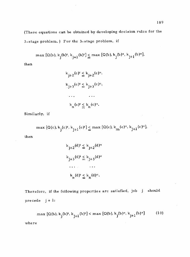
189

(These equations can be obtained by developing decision rules for the

3 -stage problem,) For the 3 -stage problem, if

max [Q(b), kj(b)°, kj+1(b)°] < max [Q(b), kj(b)", kj+1(b)1,

then

Similarly, if

then

kj+2(c)1 < kj+2(c)",

kj+3(c)1 kj+3(c)",

kn(c)° < kn(c)".

max [0(c), kj(c)°, kj+l(c)°] < max [Q(c), km(c)"°, kj+1(c),°],

k. (d)° 3+2 < k. (d)"

3+2

kj+3(d)° < kj+3(d),

,° +3td)

kn(d)° < kn(d)".

Therefore, if the following properties are satisfied, job j should

precede j + 1:

b max [Q(b), k.3 (b)°, kj +1(b) °] < max [Q(b), kj(b) kj

+1(b) °] (10)

where

Q(b) = max 1<u< j-1

kj(b)° =

i=1

j+1

bk. j+1()° ai m

b. 3+1 1

i=1 i=1

j-1

i=1

bi

kjQbpo =

kj +1(b) =

j- 1

ï =1

j+1

+ aj+1

j-1 b m bj i +1

i=1 i=1

i=1

bi

190

(12)

(13)

(14)

(15)

c k.( )'0, max [Q(c), kj(c) °, k. 3+1

(c)3] < max [Q(c), kj +1(c) "] (16)

(refer to the equations 6 to 9 and 1 above) and

d) max [k.(°, ke (d)°] +1

< max [k.(d)19, k. J+1

(d)u] (17) ,

(refer to the equations 1 to 5 above).

For a 3 -stage problem, the restrictions will be:

u u-1 [aib. _ = i=1 i=1 -

L ai

-

-

x_ 191

Condition (1):

min {bi -max [Q(b), kj(b)'], c.-max[Q(b), k.(b)", k+1(b)']} J J +1 J J

< min b. - J+1

max[Q(b), k.(b)'], ci-max [Q(b), J

kj(b)', J

k. +1 (b)']} (18)

and Condition (2):

max[Q(b), k.(b)', k. (b)o] < max[Q(b), k(b)", k (b)"] (19) J+1 = J J+1

These rules can be extended for m- stages and we note that the

m -stage rule is valid only if (m -1) conditions are satisfied.

Algorithm for the m -Stage Problem: Assume that (j -1) jobs

have been scheduled for the feasible sequence and we are to determine

the order positions of the remaining (n +1) jobs.

Step (1): Compute Si = [ai +bi +ci +... (m -1) i] for all remaining un-

scheduled jobs and determine the one with the minimum Si.

If there is a tie, choose the one with maximum m.. Place

the job in the j -th order position.

Step (2): Sequence one of the remaining (n -j) unscheduled jobs in

the (j +l)th order position. For the sake of definiteness

and to make sure that no possible sequence is overlooked,

choose the job with the smallest i first.

Step (3): Examine if Condition 1 is satisfied.

Step (4): Apply one of the following:

(a) If Condition 1 is satisfied, repeat Steps 2 through 4 for

J J

J

i

192

each possible sequence by placing each one of the un-

scheduled jobs in order position (j +1); continue to

Step (5).

(b) If Condition 1 is not satisfied because of an equality, re-

peat Steps 2 through 4 for each remaining sequence by

placing each of the unscheduled jobs in order position

(j +1); go to Step (5).

(c) If Condition 1 is otherwise not satisfied, replace the job

currently in j -th order position with the job placed in

sequence position (j +1), repeat Steps 2 through 4 for

each remaining possible sequence. If all unscheduled

jobs have been tried for order position j, go to Step

(5).

Step (5): (a) If the job currently in the order position j satisfies

Condition 1 for all remaining unscheduled jobs, go to

Step 6(a).

(b) If the job presently in the j -th order position does not

satisfy Condition 1 because one or more of the remaining

unscheduled jobs yield an equality, go to Step 6(b).

(c) If none of the remaining unscheduled jobs satisfies (a)

and (b) above, go to Step 6(c).

Step (6): (a) Examine if Conditions 2. through m -I are satisfied for

the remaining unscheduled jobs.

193

(i) If Conditions 2 through m -1 are satisfied, place

the job in the j -th order position.

(ii) If Conditions 2 through m-1 are not satisfied for i

remaining (n -j) unscheduled jobs, it is to be assumed

that the job currently in the j -th order position and

the remaining i unscheduled jobs (that do not satisfy

the condition) as the j -th job of (i +l) feasible se-

quences.

(b) It is necessary to assume the job in the j -th order

position as well as k of the remaining unscheduled

jobs as the j -th job of (k +1) feasible sequences,

where k is the number of remaining unscheduled jobs

that had yielded an equality for Condition 1.

(c) Assume that all remaining (n +l -j) unscheduled jobs

as the j job of (n +l -j) feasible schedules and go to

Step (7).

Step (7): Go to Step (1) and repeat the Steps (1) through (6) till (n-2)

order positions are determined. [If more than one job is

assumed in Step (6), the first is scheduled to order position

j and the others are put aside until Step (10)].

Step (8): To obtain a job for the (n -1)th : order position, examine

which of the two remaining unscheduled jobs satisfies Condi-

tion 1. Place the respective job in sequence position (n -1)

194

and the remaining jobs in the position n. If ties occur,

select either one for position (n -1) of the feasible se-

quence.

Step (9): Compute the total elapsed time for the feasible schedule ob-

tained in Step (8).

Step .(10): If more than one job have been chosen for position j in

Step (6), select another (the first was chosen in Step 7) and

repeat Steps 1 through 9 until all possible feasible schedules

are obtained. Compute the makespan for each of them.

Step (11): Determine the sequence (s) that has the minimum elapsed

time.

Dudek and Teuton (1964) have programmed and used an IBM

1620 in solving several 3 -stage and 5 -stage scheduling problems. It

has been found that the general algorithm generates one or more

optimal schedules; but not necessarily all possible optimal sequences

for a scheduling problem.

All m -stage scheduling problems cannot be solved using this

algorithm. Karush (1967) has presented a numerical example for

such a situation.

2. Graphical Algorithm

A graphical approach for scheduling n -jobs on m- facilities for

minimizing their make -span was first suggested by Akers (1956), and

195

later extended by Hardgrave and Nemhauser (1963).

Akers (1956) has developed a simple and efficient approach for

the scheduling of two jobs on m- machines and Hardgrave and

Nemhauser (1963) tried to extend the graphical method for sequencing

n -jobs on m- machines. However, a computational method will have

to be adopted in the n -stage problem because of the difficulty of con-

structing an n- dimensional network.

Scheduling of Two Jobs on m- machines: The algorithm is

formulated on the following assumptions:

1. The technological ordering for each job is known. They

need not be the same for both jobs.

2. No machine can process more than one job at any time.

Similarly a job can be processed in only one machine at a

given time.

3. It is not necessary that all the facilities process the jobs in

a same order.

Let

of = processing time for job in facility f.

sif = earliest start time for job i in facility f.

T. = minimum time required to complete the processing of

job i.

i

tif

..

i

196

Xi = axis for job i in the graph.

The processing times of the two jobs, job 1 and job 2, are rep-

resented respectively along the X1 axis and X2 axis as shown in

Figure 6 -14. A rectangle of width T1 and length T2 defines the

region called an outer rectangle in which any point may represent a

degree of completion of each job. The point (0,0) represents the

starting of the jobs and (T1, T2) indicates the completion of the

jobs, 1 and 2. The shaded areas in Figure 6 -14, . denotes the dura-

tion of times when both jobs require the same processing facility

simultaneously. These shaded rectangles are known as infeasible

regions.

The path represented by a continuous line consisting of vertical,

horizontal, and diagonal (45 °) segments or branches from (0,0) to

(T1, T2) is called a schedule. A schedule that does not pass through

the infeasible regions is called a feasible schedule.

The processing of job 1 only, while job 2 remains idle is rep-

resented by a horizontal line segment and the processing of job 2 only

is represented by a vertical line. A diagonal line corresponds to the

processing of both jobs simultaneously.

In computing the elapsed time, a diagonal movement over a

unit of time is equivalent to a simultaneous vertical movement for

one time unit and a horizontal movement for one time unit. Thus, in

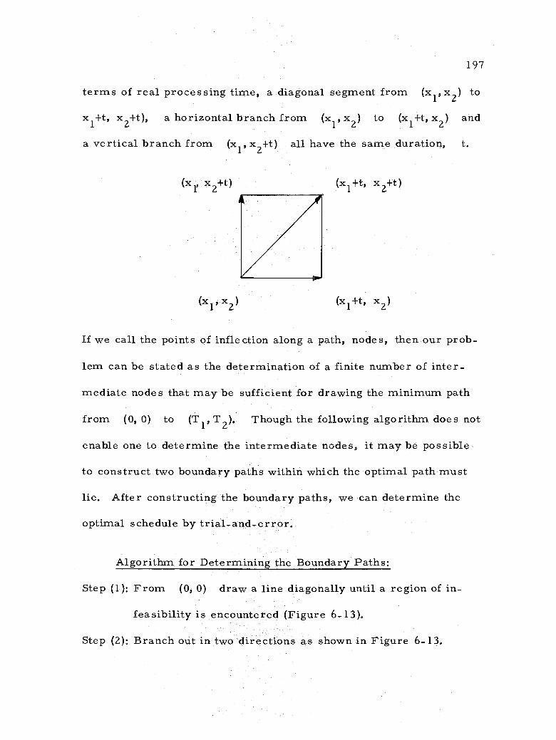
197

terms of real processing time, a diagonal segment from (x1, x2) to

x1 +t, x2 +t), a horizontal branch from (x1, x2) to (xi +t, x2) and

a vertical branch from (x1, x2 +t) all have the same duration, t.

(x, x2+t) (xl+t, x2+t)

(x1, x2) (xl+t, x2)

If we call the points of inflection along a path, nodes, then our prob-

lem can be stated as the determination of a finite number of inter-

mediate nodes that may be sufficient for drawing the minimum path

from (0,0) to (T1, T2), Though the following algorithm does not

enable one to determine the intermediate nodes, it may be possible

to construct two boundary paths within which the optimal path must

lie. After constructing the boundary paths, we can determine the

optimal schedule by trial- and -error.

Algorithm for Determining the Boundary Paths:

Step (1): From (0,0) draw a line diagonally until a region of in-

feasibility is encountered (Figure 6 -13).

Step (2): Branch out in two directions as shown in Figure 6-13.

198

Figure 6 -13. An illustration of constructing the paths.

Step (3): Extend the diagonal line until a region of infeasibility is

again encountered. Go to Step (2).

Continue the same procedure till the top or right edge

of the outer rectangle is reached. Extend the line along that

edge to the point (T1, T2).

We obtain two or more paths connecting the starting and

completion nodes.

A L.

199

Step (4): Starting from the completion node, (T1, T2), follow the

steps 1 through 3, to construct two or more paths connecting

the completion point to the starting point. (In this case, the

nodes (0, 0) and (T1,T2) are interchanged from Step 3,

and path drawn backwards. )

Step (5): Choose two sets, P1 and P2 of branches (among the

available paths) which are in the innermost portion of the

paths as shown in Figures 6-14 and 6 -15. These two sets of

branches form the bounds for the optimal path. The optimal

path must lie on or inside the two bounds, P1 and P. Step (6): Consider as many feasible sequences as possible in the

region and compute their corresponding elapsed time. The

one with the least value is the optimum schedule.

Example: The technological order of processing jobs 1 and 2

and their processing times in days are known. Determine in which

order the planning department should sequence them so that the make

span is minimized.

Job 1: A(4)-C(1)-B(3)-E(2)-G(1)-F(3).

Job 2: A(3)-C(3)-B(6)-G(1)-E(3)-F(2).

We follow the constructional procedure to find the paths (Figure

6 -14) and determine the boundaries P1 and P2 as shown in

zoo

Figure 6 -14. Graphical method for determining the boundaries.

B -0.-- 1-0-- E G F -

Job l X1 axis

10

E

G

G

A

10

s

/ / /

f

\\\N' (o,p) I- A

/

/

.

f

/

Lft /

/ /

/

/ / / /

/ V /

I

201

Figure 6 -15. Graphical method for determining the optimal sequence.

A B

10

E H G F

Figure 6 -15. The boundary P

elapsed time is 22 days.

2 is an optimal schedule and the

202

Scheduling n -jobs on m- machines: The graphical n -jobs on m-

machines algorithm is based on the assumptions stated under the

scheduling of two jobs on m- machines.

The feasible and the infeasible regions of an n -stage scheduling

problem, may be considered to be the parts of an n- dimensional rec-

tangle which may be defined by 0 < X. < Ti for i = 1, 2, ... , n.

For n -jobs in a facility f, there are C2 blocks representing n

infeasible regions.

The method of branching out can be as follows:

1. From (0, 0, 0, ... , 0) proceed diagonally until an infeasible

region is encountered.

2. Whenever an infeasible region is encountered, branch out

around it in n possible ways (refer to Figure 6 -13 for

n = 2).

3. Along these branches move "diagonally" until another in-

feasible region is encountered. Go to (2).

Similarly, start from (T1, T ... , Tn) and draw the

paths to the origin (0, 0, 0, , 0).

The boundaries can be determined and by trial -and-

error, the optimum schedule may be determined.

203

Hardgrave and Nemhauser (1963) have presented a proof show-

ing that a sequence with the shortest elapsed time can be obtained for

the general problem using this graphical approach.

3. Programming Methods

The research on the general scheduling problem has resulted in

several linear programming models.

The schedule of a task has been represented as a network by

Dantzig (1960) and he had formulated a linear programming model

for obtaining the optimal schedule that minimizes the make span. A

weakness of the model is that in some situations the optimum schedule

obtained is not feasible.

Bowman (1959) and Wagner (1959) have established integer pro-

gramming models and Manne (1960) has constructed a mixed linear

programming model.

The experimental results of Giglo and Wagner (1964) show that

only a very limited number of positive results has been obtained by

the integer programming approach. At least for the time being, our

interest in these models tends to remain more theoretical than prac-

tical.

(a) Linear Programming Model. Dantzig (1960) has formulated

a linear programming model for the machine -shop scheduling prob-

lem and it is based on the network flows.

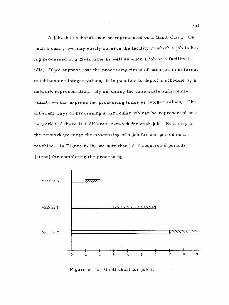
204

A job -shop schedule can be represented on a Gantt chart. On

such a chart, we may easily observe the facility in which a job is be-

ing processed at a given time as well as when a job or a facility is

idle. If we suppose that the processing times of each job in different

machines are integer values, it is possible to depict a schedule by a

network representation. By assuming the time scale sufficiently

small, we can express the processing times as integer values. The

different ways of processing a particular job can be represented on a

network and there is a different network for each job. By a step in

the network we mean the processing of a job for one period on a

machine. In Figure 6 -16, we note that job 7 requires 6 periods

(steps) for completing the processing.

Machine A

Machine B

Machine C V

0 1 2 3 4 5 6 7 8 9

Figure 6 -16. Gantt chart for job 7.

205

This may be represented by the network as shown in Figure

6 -17. It has been assumed that the maximum number of time periods

including delays required to complete the job 7 is 9 periods. In the

network representation each downward arc for a particular facility

indicates a specific step done at a particular time and each horizontal

arc denotes a possible period of delay. As each path indicates a

schedule from the source to the sink along the arrows there are o

(6) = 84 possible schedules for job 7. In the linear programming

model, each path (schedule) is represented by an activity.

Example: Let us illustrate the formulation of a linear pro-

gramming model by a simple example. Two jobs, J1 and J2 are

to be scheduled in two machines, M7 and M8 and their techno-

logical processing order and processing times are given. The cri-

terion is to minimize the makespan.

M7(1 period) - M8(1 period)

J2 - M8(1 period) - M7(1 period).

The upperbound for the maximum time required to process the jobs

is 4 periods (being the sum of all processing times).

In Table 6 -21, the columns y1 through y6 depicts the pos-

sible ways of sequencing J1 in the 4 time periods and columns

through y12 represents, similarly, the 6 different ways of

Y7

J1 -#

Source

Machine A (Step 1)

Machine B (Step 2)

Machine B (Step 3)

Machine B (Step 4)

Machine C (Step S)

Machine C (Step 6 )

I

0 1 2 4 5 6 7

Figure 6 -17. Network representation for the schedule of job 7.

Sink

I I I 1

3 8

scheduling

notes that J2

207

in 4 time periods. For instance, column y11 de-

may be scheduled in M8

in time period 2 and in

M7 in time period 4. Only one among the -six schedules for J1

(y1 to y6) shall be chosen due to the constraint 1. Similarly

only one of the possible schedules for J2 will be selected because

of the constraint 2. If the results of the linear programming model

is y. = 1, we choose the schedule y. and if yk = 0, we dis- J

card the schedule yk.

Table 6 -21. Linear programming model.

1

Schedules for J1 Schedules for J2

y1 y2 y3 y4 y5 y6 y7 y8 9 y10 y11 Y.

1 J1 1 1 1 1 1 1 = 1

2 J2 1 1 1 1 1 1 = 1

3 M7 1 1 1 1 1

4 2 1 1 1 < 1

5 3 1 1 1 < 1

6 4 1 1 1 < 1

7 M8 1 1 1 1 <1

8 2 1 1 1 < 1

9 3 1 1 1 < 1

10 4 1 1 1 Z 1

(Z) 1 1 1 1 1 1 = Z(min)

To start with, we wish to see if the use of the machines during

period 4 may be eliminated. This is done by minimizing the sum of

those schedules (activities) that use the machine for period 4. If the

value of the objective function is zero, then these schedules are

J2

J

208

discarded and the objective function is changed to minimize those

schedules requiring the machines for the period 3. Thus at each

stage, the elapsed time is reduced by one unit period and the same

procedure is continued until it is not possible to obtain the value of

the objective function as zero. The sequence we have obtained in the

last step is the optimal schedule.

This linear programming model does not ensure that in all

situations we shall obtain integer values for the activities,

For instance, for J1,

yj.

scheduling 1/4 of it according to y4 in

the different facilities and 3/4 of it according to y5 in the same

facilities is not practicable in most of the situations. In these cases,

integer linear programming solutions must be used.

(b) Integer Linear Programming Models.

Algorithm by Bowman. Bowman (1959) has formulated a linear

programming model for the general job -shop scheduling problem to

establish the optimum sequence that minimizes the makespan.

Assumptions: The model is constructed on the following as-

sumptions:

1. The processing times for each job are integer values.

2. The order of processing each job on different facilities is

known.

3. At a given time, any job can be processed on one and only

209

one facility.

4. Once a machine has started processing a job, the operation

is continued, without interruption, until the completion of

processing in that machine.

We shall illustrate the formulation of the model by a numerical

example.

Three jobs x, y, and z are to be sequenced in the facilities

1, 2 and 3. The facility sequence matrix, F, specifies the order

in which each job is processed in the machines. The processing time

matrix, P, denotes the periods required by each job for process-

ing in different machines. For our example, suppose

F = Y 1 and P = y 2 0 0

(hours) 2 Z = 3 1 0

Let

x. j,

= job x having machine operation j during time per -

iod i.

= 1 --R if it is true.

= 0 if it is not true.

T = time period considered within which all operations can

be completed.

X --r. 2 3 X -P" 2 3 0

-

1

210

The value of T may be taken as the sum of all processing

times as within this period of time all the operations can be completed

(even in the worst case). Therefore, T 11 hours.

Constraints:

(i) Constraints to ensure that all operations are done on each

job in different facilities. The form of the restrictions are:

for job x:

for job y:

for job z:

11

in machine 2, J x2, = 2

in machine 3,

i=1

11

yl,i

i=1

11

i=1

zl, = 3 i

=

i=1

11 / x3 i

= 3 .

1 = 2

/ 11

1 z2, = 1

i=1

i

211

(ii) Constraints to assure that at any specified period of time

each machine either processes one and only one job or is

idle.

For facility 1,

For facility 2,

For facility 3,

y19 1

+ z

< 1 19

y192+z < 1

yl, 11 + z1, 11 < 1

x291 + z2, 1< 1

x2911 +z2,11< l

x391< 1

x3,2< 1

x39 11

< 1.

If the left side of the inequality for the facility j during

the time period t is 1, the facility j is in its pro-

cessing state during the period t and if it is 0, the

facility is idle.

(iii) Constraints to ensure that each job is processed in the

proper order (as stated in the F matrix) in different ma-

chines.

212

Job x must be processed for 2 hours in machine 2 before its

operation on machine 3 can be started. This property can be satisfied

with the aid of the inequality:

2x3, j<

(j- 1

i=1

for j = 1,2,3,...,11.

Let us consider the following two schedules (S1 and S2).

Schedule, S1

Schedule, S2

B B C C C

0 2 3 4 5 6 7 8 9 10 11

Figure 6 -18. Gantt chart for schedules of job x.

Substituting the values of x 2, i

and x 3, j

in the constraint

for schedule S, we note that it holds for all j values except for

j = 5. On the other hand, the schedule S2 satisfies the constraint

for all j values. Therfore, we may conclude that the above form

of constraint can be fulfilled only by those schedules that agree with

the F- matrix for that particular job.

x2, ' LLL

C C

0

1.11%. ÚMIIIM = 1 2 3 4 5 6 7 8 10 11

For job z,

3z < ) z for j = 1,2,3,...,11. 2,J=

i =1

213

(iv) Restrictions to guarantee that once the operation has been

started by a facility on a job, it is continued in that facility

until the completion of the process. Thus, no interruption

is allowed in a facility while it is processing a task.

For job x,

11

2x2, i

2x2, i+1 + L j

x < 2

j=i+2

3x 3x + 3, i+1

11

j=i+2

< 3

for i = 1, 2,3,..., 11.

Substituting the values of the schedules S3 and S4 (Fig-

ure 6 -19), we observe that the above form of restrictions

hold only for those machine operations that are processed

uninterruptedly. For S3, the property is not true for

i = 4 and for the rule holds for all i values.

-

i

S4,

,7_1

' i

-

2,

_

Schedule, S3

Schedule, S4

214

0 1 2 3 4 5 6 7 8 9 10 11

Figure 6 -19. Gantt chart for schedules of job x.

Similarly, for, job y,

11

2y1, 2yi, i+1 + yi j< 2

j=i+2

and, for job z,

11

3z1 i- 3z1 i+1 +

z < 3 9 aJ=

j=i+2

for i = 1, 2,..., 11.

(v) The decision variables shall take the values 0 or 1.

Hence, the form of the constraints are

1 > X ,X ,...,z > 0. 2,1 2,2 2,11=

Objective Function: The criterion is to minimize the makespan

(total elapsed time). We observe that in processing the three jobs,

0 2 3 4 5 6 7 9 10 11

)

3 J 1 1\\\\f\\\ M I 1 1 1 I

1 8

I.a\\\l.\\\\ I I I I 1

- -

215

the job x requires the maximum time (5 hours) and it is not pos-

sible to construct a schedule with an elapsed time of less than 5 hours.

We wish to minimize the period that is likely to be used beyond 5

hours. This is done by assigning to each operation a synthetic cost

for each unit of time this lower bound value (5 hours) is surpassed

and minimizing this cost function. The cost for an operation in a

time period may be taken as equal to the sum of all prior costs plus

one. Therefore, the objective function is

minimize C = 1 (x3, 6 +y1, 6 +z2, 6) + 4(x3,

7 +y1, 7 +z2, 7)

+ 16(x3, +yl, +z2, 8) + .. .

+ 45(X3, 11 +y1, 11

+z2, 11)

The total number of decision variables for a job -shop scheduling

problem, depends on the number of jobs to be processed, facilities

to be used and also the number of time periods chosen. Even for a

problem of modest size, the computation required appears to be quite

large.

Algorithm by Manne. Manne (1960) has formulated a mixed

linear programming solution for establishing the optimal sequence of

n jobs on m machines. The criterion is to minimize the make -

span.

In the mixed linear program some of the variables are

8

216

constrained to be integers. Although an efficient computer program

is still not available, this mathematical model is of interest, at least

for the time being, from a theoretical point of view.

Let

si. = the start time of job i on machine j J

t.. = the processing time of job i on machine j iJ

f.. = the fraction of job i completed on machine j before ijr

another job r is started on the same machone (integer

value)

= 1 if job i precedes job r

= 0 if job r precedes i

t = total elapsed time to complete all operations.

Constraints:

(i) Technological constraints: The operation on job i on

machine j must be completed before it is started on the

next machine, say k.

sik.> si, + ti.

J 13

Such restrictions are to be constructed for all jobs and

machines taken in pairs of next following facilities. For an

n -job and m- machine scheduling problem we have n(m -1)

restrictions.

=

217

(ii) Noninterference constraints: These restrictions are intro-

duced so as to ascertain that a job i is completed in

machine j before another job, say r, is started in j;

that is, at any given time, the machine j is processing

not more than one job. Set a large value for T, say

/t.., then ) s.. - s !

< T. and also 1) i) rj

(sij -srj) + fijr(T+trJ) > trJ

(s .-s..) + (1-f.. )(T+t..1> t.. r 13 ijr 13)= 13

If i precedes r, then f.. = 1 and the two restrictions ijr are satisfied. On the other hand, if r precedes i, then

f. = 0 and the two restrictions are satisfied. The two iJr

constraints cannot be simultaneously fulfilled unless the

operation on the first job is completed. For an n -job and

m- machine problem, we have n(n -1)m /2 such inequalities.

(iii) Completion time restrictions: The time of completion of all

operations must be at least equal to the completion time of

the last job on the last facility. Hence,

t > s.. + t.. for all i and j. -

We have mn equations of this type for an n -job and m-

machine problem to ensure that the completion time

13 li

218

constraint is satisfied.

(iv) All the decision variables are non -negative.

s.., t.., f.. > 0 for all i, j and r. i i ijr -

Objective function: The total elapsed time is to be minimized.

Therefore,

minimize: t

If there are n jobs to be sequenced on m facilities, the number

of variables would come to mn for s.. and n(n -1)m/ 2 for 13

f.. and 1 for t. For instance, even in a small problem with ijr five machines processing all the ten jobs, there would be 276 deci-

sion variables in the mixed linear programming model.

Algorithm by Wagner. Wagner (1959) has established an inte-

ger linear programming model for the job -shop scheduling problem

and it is adaptable to a large number of sequencing situations. We

present an algorithm by Wagner (1959) for determining the optimum

schedule that minimizes the total elapsed time required to process

all the jobs. It is required, in this model, that the order of manu-

facturing for each job is machine 1, machine 2, ... , machine m.

Let

1 if job i is scheduled in order -position k on (j) 1 machine j ik

otherwise 0

Z19

b(i) = time at which the job sequenced in the order -position k

begins processing in machine j.

s» = time elapsed on facility j between the completion of the

job sequenced in the k -th order -position and starting

of processing the job scheduled in order -position (j +1).

s ÓJ) = time elapsed on machine j between the beginning of

manufacturing (in machine 1) and the start of processing

in the order -position 1.

tx(i) = processing time of job scheduled in order -position k on

machine j.

d(i) = time elapsed between the completion of processing the job

scheduled in order -position k on machine j and the

starting of the job scheduled in order - position j on

machine (j +1).

The values of all above variables are nonnegative integers.

The job i is said to be scheduled in the order -position k on

machine j, if prior to scheduling this job on the machine j, (k -1)

jobs have previously been processed on it.

Each job must be processed in some order- position and there-

fore, we have the constraint;

/xik = 1 for all i.

k

(1)

Because there is some job in each order position, we have,

L xik 1 for all k

i

220

(2)

The job at order - position k on machine (j -1) cannot be

completed after the starting of the job at order -position k on ma-

chine j.

b(J) b(J-1) 1)+d(J 1) (3) k k k k

b(1) = b(1) + tx(J) + s (i) (4) k (k-1) (k-1) (k-1)

from (3) and (4)

0 = b(i) - b 0-1) + tx(J) (k-1) k (k-1 (J-1) s(J) (j-1) - tx(J + s dk

Suppose that the job i is scheduled in order -position k' on

maching j1 and in order - position k" on machine j2. Then,

0 - tx(J) - tx(j'-1) s(j') s(j`-1) d(j-1) _ d(J-1) k' k'+1 k' k' k' (0+1)

1 <j' <m, 1<k'+1<n

(5)

There are (m -1)(n_ 1) relations of this type to ensure that this con-

straint is satisfied. From Johnson (1954), we obtain the equation

(1)_d (1)(m 1) k 1 1

=

(k-1) k

ski _

0

221

The objective function is to minimize the total elapsed time. As each

job is processed in the order machine 1, machine 2,.,..,., machine m,

the total elapsed time =

But,

k =1

x.lm) + sóm) + sim) +. . . + sñmi

txkm) = constant.

k==1

Therefore, the objective function is

minimize sum) (m)

+ sim) + ...+ snml .

A special case of this algorithm for three stage scheduling

problems is described in Chapter V -A -2.

C. Total Cost (Production and Storage Cost)

Because of the restrictions imposed by constant changes in the

availability and prices of such resources as labor, materials,

machine hours, storage facilities and market requirements, many

manufacturing firms are confronted with periodic fluctuations in pro-

duction, in inventory, or in some combination of the two. In these

situations, the problem may be conceived that requires the deter-

mination of the production schedule that minimizes the sum of

n

n

222

production costs (on regular time and on overtime) and the inventory -

storage costs.

Bowman (1956) has formulated a transportation method of linear

programming for establishing the optimum schedule that minimizes

the total cost.

Vazsonyi (1957, 1958) has developed a computational method

for obtaining a feasible schedule that satisfies the sales requirements

with the available labor and machine hours.

1. Transportation Method

The transportation model established by Bowman (1956) for de-

termining the optimal schedule for future time periods that minimizes

the sum of production costs and inventory- storage costs requires the

following assumptions:

1) The number of units of finished product to be sold in the

future time periods are known.

2) The maximum number of jobs which can be produced during

each time period (on regular time and on overtime), cost of

production per unit during each time period (on regular time

and overtime) are given.

3) The number of items required, if any, in inventory at the

end of the last time period (n) is known.

4) The cost of storage per unit per unit time for each time

223

period is known.

The scheduling problem may be formulated as a transportation

problem considering each type of manufacturing, regular or over-

time, in each time period as a source of supply or input. Each time

period's sales requirement is considered as a warehouse or output.

The unit cost of shipment may be viewed as the sum of production

cost and storage cost, as depicted in Table 6 -22.

Let,

x pir = maximum number of units of product p which can be

manufactured during i -th time period on regular

time.

xpi0 = maximum number of units of product p which can be

manufactured during i -th time period on overtime.

y = number of units of product p required by sales depart - Pj

ment during the j -th time period.

I = number of units of product p required in inventory at Pj

the end of time period j.

C pir = cost of producing one unit of product

period on regular time.

in the i -th

Cpi0 = cost of producing one unit of product p in the i -th

time period on overtime.

S P

= cost of storage per unit of product p in the time per -

iod t.

p

Table 6 -22. Unit costs of shipment for product 1.

i p

Sales period, j

2 k

0 Inventory 1 0 S11

(k-1)

Slt t=1

R. T.

O. T.

1

1

Cllr

C110

Cllr + S11 + S11

C110+S11

'

'"

k-1

Cilr+ L Slt t=1

k-1

CI10+ Slt t=1

2 R. T.

O. T.

1

1 -

C12r

C120

°

.

k-1

C12r+L Slt t=2 k-1

C120+/ Slt t=2

k R. T.

O. T.

1

1 --- Clkr C1k0

Total requirements y11 y12 ylk

R. T. denotes regular time. O. T. denotes overtime.

Total Inventory (k) Slack capacities

Slt t=1

0 I10

k

Cllr+ L Slt Xllr t=1 k

C110+ L Slt t=1

X110

C

C120+

1

k

0

X12r

X120

Clkr + Slk

C1k0 + Slk 0

Xlkr

XlkO

Ilk Q

Q = total slack = I10 + Exlir + XIi0 - Zylj - Ilk

1

k

1

0

- LJ lt t=2 k

LJ It t=2

0

- "' ..

0

225

It is not possible to produce the units in one period and sell

them in a previous period. Therefore, the cells which hold the prop-

erty i > j, are denoted by a dash.

In Table 6 -22, the transportation model is formulated for

scheduling the manufacturing and sales quantities of product 1 for

k -time periods assuming that the production costs (on regular time

and overtime) and storage costs are not the same in different periods.

The problem of scheduling n products can be formulated as fol-

lows: for each sales period, the requirement of these n products

are to be considered; that is in the Table 6 -22, under each period

j, n columns are to be constructed. Similarly, in each production

period, the manufacturing of the n products is to be considered.

Elmaghraby (1957) has commented that if the cost of regular

production, the cost of overtime production and the cost of inventory

per unit are constant, we do not have to formulate the transportation

model. By adherring to the rules, "produce as late as possible to

satisfy the demand and do not produce on overtime except when you

cannot produce on regular time before, " the optimal schedule can be

established without much computational effort and also the 'feel' for

the problem would not be lost.

2. Allocation of Machine -Hours

Vazsonyi (1957, 1958) has formulated a technique for scheduling

226

job amounts to be manufactured in different production periods so that

the shop may be able to meet the requirements. The objective is to

minimize the combined cost of setups and inventory carrying. The

computational method does not enable one to determine the optimum

schedule (manufacturing quantities of different jobs) but it is possible

to determine the order quantities so that the requirements are met

with available labor and machines.

The following assumptions are necessary in using the algo

rithm:

1) The requirements of each job for the future production per-

iods are available.

2) For each machine, the total machine hours available in the

production periods are known.

3) The production shop has enough experience from past per-

formance to predict the fraction of time each machine needs

for processing the jobs (in the remaining time, the machine

is either idle or it is being arranged for the next job).

Let

J1, J2, ... , Ji... jobs to be produced.

M1, M2, ... , Mf... = machines to be used for processing.

PP2,..., Pk. .. P = production periods. P

rk) = unit requirement of job i in production per- i

iod Pk.

=

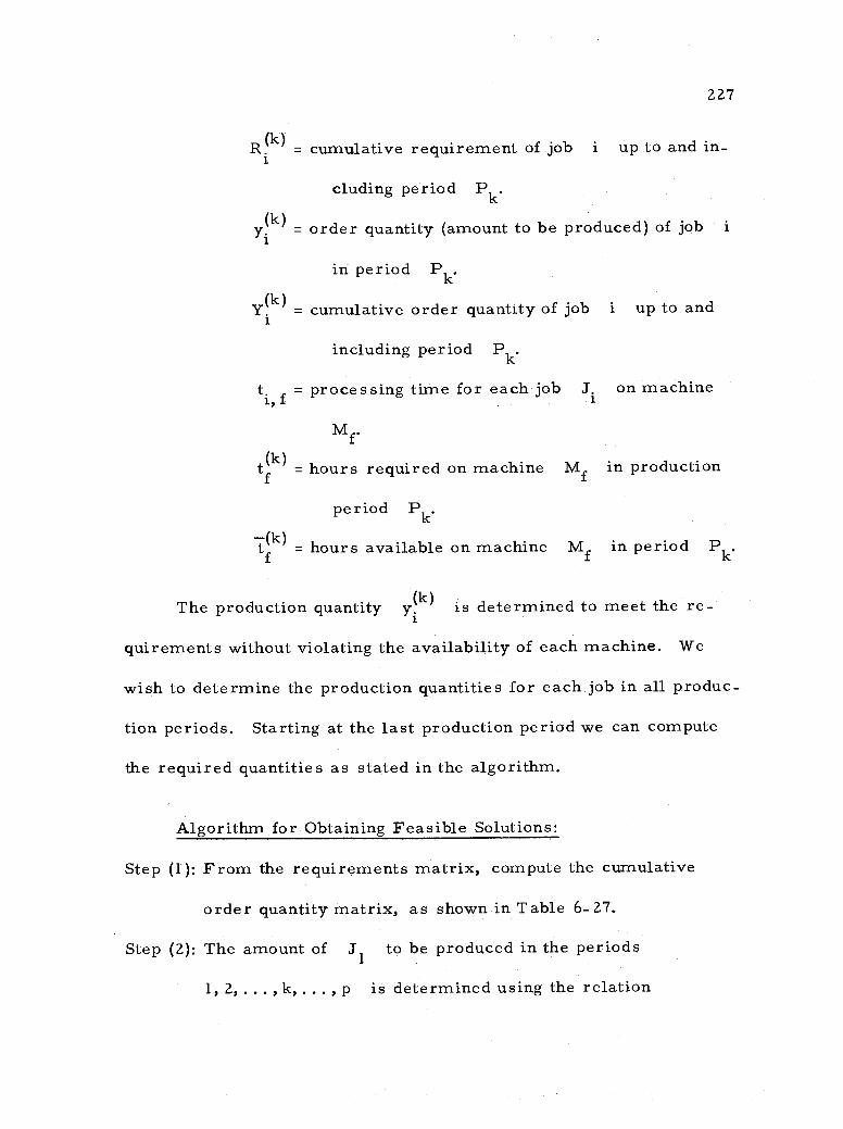
(k) = cumulative requirement of job

cluding period Pk.

227

up to and in-

y(k) = order quantity (amount to be produced) of job i

in period Pk.

Y(k) = cumulative order quantity of job up to and

including period Pk.

ti = processing time for each job Ji on machine

Mf.

t(k) = hours required on machine Mf in production

period Pk.

t fk) = hours available on machine Mf in period Pk.

The production quantity y(k) is determined to meet the re-

quirements without violating the availability of each machine. We

wish to determine the production quantities for each job in all produc-

tion periods. Starting at the last production period we can compute

the required quantities as stated in the algorithm.

Algorithm for Obtaining Feasible Solutions:

Step (1): From the requirements matrix, compute the cumulative

order quantity matrix, as shown in Table 6 -27.

Step (2): The amount of J1 to be produced in the periods

1, 2, ... , k, ... , p is determined using the relation

i

i

228

=Y. max Yik 1) max [Yik) -min f(t fk) /ti} f)]; Rik 1)

(k = p,p-1,p_2,... )

where i = 1.

Step (3): Compute xfki for each facility using the rule:

(k) (k) xf, fy1

ti, '

where xfki = load imposed on facility f in the period k

9

by scheduling only one part. Similarly xfki is calculated 9

for each production period.

Step (4): Compute the machine hours that are still available after

scheduling only one part (job J1) with the aid of the for-

mula

(k) = t (k) (k) f, 1 f f, 1

Construct the 'available hours' matrix z(f )1 as shown in

Table 6 -29.

Step (5): The order quantities for J2 are computed using the rule:

Yik 1) max [Yik) -min f(zfki /ti f)3 RI

1) > >

(for k = p, p-1, p-2, . . . ) and i = 2.

We note that we have replaced the originally available hours

(k) z by the balance of the hours, f, l'

.

z

=

_

f

229

Calculate the hours imposed on the machines by J1 and

J2 with the aid of the equation

(k) (k) (k) xfe2 =t19f y1 +t2,f y2

The balance of available hours matrix is obtained with the

aid of the equation:

(k) = t -(k)

(k) z f,2 f x f,2

For computing the schedule for J3, use the formula:

Y(3k 1) =maxi [Y3k)- rninf(z 2/t3, f)], k-1)1

(for k p,P-1,...).

The same procedure is repeated till all the n jobs are

scheduled in all production periods.

In the above method of solution, we have first computed the

schedule J1, then J2 and so on. In the alternate method of solu-

tion, we may start by scheduling J1 in the last period, then sched-

uling J2 also in the last period, and so on till all the jobs in the

last production period have been scheduled. Then, we proceed with

the scheduling of all the jobs in the next to the last production period

and so on until we have scheduled all the jobs in the future periods

available. However, the amount of computations involved seems to be

2 ,

=

230

equivalent in both of these methods.

Example: The sales dapartment of a diesel engine manufactur-

ing company has informed the production department of its require-

ments for engine types J1, J2, J3 and J4 for the periods P3,

P4' P5' P6 and P7. These are shown in Table 6-23. The total

available facility hours in machines M1, M2 and M3 are given

in Table 6 -24. From the past performance, the production personnel

predict that M1 shall be in production for 75% of the available

machine time, M2 for 75% of the time, and M3 for 80% of the

time. The production control department wishes to obtain a schedule

so that it can meet the sales department's requirements with avail-

able machine hours.

Table 6 -23. Requirements of sales department (r(k)1 ).

P4 P5 P6 P7 Inventory

J1 0 0 200 400 400 0

J2 100 100 200 300 0 0

J3 0 0 0 0 200 100

J4 100 100 100 100 100 0

Table 6 -24. Total machine -hours available (hours).

f P3 P4 P5 P6 P7

M1 1600 1600 1600 1600 1600

M2 1600 1600 1600 1600 1600

M3 2500 2500 2500 2500 2500

i \ P3

231

Table 6-25. Run time matrix (ti f) (hours).

f J1 J2 J3 J4

M1 0 4 3 1

M2 2 0 3 1.5

M3 5 2 0 3

With the aid of the relation

Available productive hours (tfk))

= (total hours available) (% of time in productive state)

we obtain the Table 6-26.

Table 6 -26. Available productive hours matrix

(tfk) ).

P3 P4 P5 P6 P7

M1 1200 1200 1200 1200 1200

M2 1200 1200 1200 1200 1200

M3 2000 2000 2000 2000 2000

From Table 6 -23, we get the values for the cumulative require-

ment matrix R (k) as shown in Table 6- 27.

Nk f

232

Table 6 -27. Cumulative requirement (R(k)) matrix.

i P3 P4 P5 P6 P7

J1 0 0 200 600 1000

J2 100 200 400 700 700

J3 0 0 0 0 300

J4 100 200 300 400 500

The scheduling of J1 for a new production period is accom-

plished as follows:

Period, P7: The value of

For M1, [0]

For M2, [2]

For M3, [5]

yi7) is such that

[y17)] < 1200

°° [y17)] < 1200

[y17)] < 1200

and substituting these values in the equation

Yik 1) max [Yik)-minf(tfk)/ti9 f)]; Rikm1)

9

(Yik) = Rik) when k = p)

Y(6) = max [1 000 -min( 1200 1200 2000 )], 600 1 0 ' 2 5

= 600.

(7) (7) (6) - yl - Y1 Y1

= 1000 - 600 = 400 units of J1

=

'

\

l JJJ

.

233

For period, P6:

Yi 5) 1200 [600- 1200 2000 200 = max .j min(

0 2

= 200

(6) (6) (5) Y yl = YI Y1

= 600 - ZOO = 400.

For period, P5:

1200 1200 2000 ' Y(4) = max [200- min(

' ' 1 0 2 5 .}

= 0

y1 4) = 200 - 0 = 200 of J1

The hours imposed by J1 is shown in Table 6 -28 and the balance

of available hours in Table 6,-29.

Table 6 -28. Hours imposed by J1 matrix

for xf kY

P3 P4 P5 P6 P7

M1 0 0 0 0 0

M2 0 0 400 800 800

M3 0 0 1000 2000 2000

' ' 5

-

J

234

Table 6-29. Balance of available hours -

matrix z . fkl

f P3 P4 P5 P6 P7

M1 1200 1200 1200 1200 1200

M2 1200 1200 800 400 400

M3 2000 2000 1000 0 0

Similarly, the order quantities for J2, J3 and J4 are com-

puted and tabulated as represented in Tables 6 -30 to 6 -35.

Table 6 -30. Hours required by J2. Table 6 -31. Balance of available hours.

Matrix z(f )).

f

k

P3 P4 P5 P6 P7 f

k

P3 P4 P5 P6 P7

M1 400 1200 1200 0 0 M1 800 0 0 1200 1200

M2 0 0 0 0 0 M2 1200 1200 800 400 400

M3 200 600 600 0 0 M3 1800 1400 400 0 0


Matrix z(k). f, 3

f P3 P4 P5 P6 P7 P3 P4 P5 P6 P7

M1 300 0 0 300 300 M1 500 0 0 900 900

M2 300 0 0 300 300 M2 900 1200 800 100 100

M3 0 0 0 0 0 M3 1800 1400 400 0 0


Matrix zf4.

P3 P4 P5 P6 P7 f P3 P4 P5 P6 P7

M1 500 0 0 0 0 M1 0 0 0 900 900

M2 750 0 0 0 0 M2 150 1200 800 100 100

M3 1500 0 0 0 0 M3 300 1400 400 0 0

\

f

k

235

We have obtained a feasible schedule (Table 6 -36) satisfying the

requirements of the sales department with the existing labor and

machine availabilities.

Table 6 -36. Order quantity matrix [Y.(k)].

i k

P3 P4 P5 P6 P7

J1 0 0 200 400 400

J2 100 300 300 0 0

J3 100 0 0 100 100

J4 500 0 0 0 0

236

VII. CONCLUSIONS

Most of the presently available mathematical models that have

been studied are summarized in Table 7 -1. It includes our own con-

tribution of two computational methods: a linear programming model

to minimize the makespan on m- 'not -alike' single -stage machines

(Chapter II- Section D -2), and an application of the branch - and -bound

technique for a set of non - repetitive jobs (open path) on a single -

stage (Chapter III -Section A -2b).

In Table 7 -1, the blocks that are not filled indicate the areas

where no computational methods seem to have yet been formulated.

For large size problems, specially for m > 3, many of the algo-

rithms impose an impressive computational load. At least for the

time being, some of them appear to be of interest only from a the-

oretical point of view. It is hoped that investigations may be carried

on to result in more efficient algorithms requiring only a practical

amount of computational efforts. Because of the computational diffi-

culties associated with present techniques in the multi -stage sched-

uling problems, heuristic methods for establishing near -optimal

sequences must not be overlooked. The cost gained by improving the

schedule must at least balance the cost spent for the computational ef-

fort, and the overall gain be maximized.

In Chapter III- Section A -1, we have presented an algorithm for

237

scheduling a set of repetitive jobs on a single stage (branch and bound

technique by Little et al. , 1963). In this situation, we have used the

algorithm for the assignment problem first and only when the optimal

assignment is not a feasible schedule, we have applied the computa-

tional method for the travelling salesman problem. Further investi-

gations may be directed in trying to obtain the optimal sequence from

the optimal assignment (even when this is an infeasible schedule) with

a minimum computational effort.

In Chapter IV- Section B -3 we have presented a generalized

Johnson's rule for job -lots by Jackson (1956). This computational

method for the two -stage problem requires more storage space than

that would be required by the Johnson's rule. Further research may

also be directed to develop a computational method for the generalized

situation with the restriction for storage space between the facilities.

The combinatorial analysis may be helpful for this situation.

For the general three -stage problem, processing time matrix

may be constructed by using random numbers, all possible sequences

(n!) may be computed and the optimal solution(s) may be selected

for different cases, such as those, including jobs with a, < b, > c,, l 1 1

a. > b. > c. and a. < bo < c.. By solving many problems for all the

possible cases, the results may be analyzed and we may see if, by

combinatorial analysis, the optimal or near - optimal schedule can be

established with less computational effort for the classic three -stage

i

238

scheduling problem.

"Time" remains the one dimension our civilization has not yet

learned to reverse the flow. In a manufacturing problem where re-

sources are subjected to various transformations, the ordering of

tasks and transformations in the time domain will remain the central

problem of manufacturing planning as long as this restriction exists.

Much work has been accomplished to solve the scheduling prob-

lems, but they are only the foundation on which more work must still

be attempted.

It is hoped that this thesis may serve as a small guide post

summarizing where we have been and pointing us the directions we

must pursue.

239

BIBLIOGRAPHY

Akers, Sheldon B. , Jr. 1956. Letters to the editor: a graphical approach to production scheduling problems. Operations Research 4:244 -245.

Akers, Sheldon B. and Joyce Friedman. 1955. A non -numerical approach to production scheduling problems. Operations Re- search 3 :429 -442.

Andrus, W. E. and A. L. Becker. 1959. A production schedule computed on the IBM -701. In: Analysis of industrial operations, ed. by E. H. Bowman and R. B. Fetter. Homewood, Ill. ,

R. D. Irwin. p. 244-254. (Reprint of IBM Technical Report no. 105, 077, 273)

Bishop, George T. 1957. On a problem of production scheduling. Operations Research 5:97 -103.

Bowman, Edward H. 1956. Production scheduling by the transportation method of linear programming. Operations Research 4:100 -103.

1959. The schedule - sequencing problem. Oper- ations Research 7:621 -624.

Brooks, George H. and Charles R. White. 1965. An algorithm for finding optimal or near optimal solutions to the production scheduling problem. The Journal of Industrial Engineering 16 :34 -40.

Churchman, C. West, Russel L. Ackoff and E. Leonard Arnoof. 1957. Introduction to operations research. New York, Wiley. 645 p.

Dantzig, George B. 1960. A machine -job scheduling model. Man- agement Science 6 :191 -196.

1960. On the shortest route through a network. Management Science 6 :187 -191.

Dantzig, George B. , R. Fulkerson and S. Johnson. 1954. Solution of a large travelling salesman problem. Operations Research 2 :393 -410.

240

Dudek, Richard A. and Ottis Foy Tenton, Jr. 1964. Development of M -stage decision rule for scheduling n jobs through M- machines. Operations Research 12:471 -497.

Elmaghraby, Salah E. 1957. A note on production scheduling by the use of the transportation method. Operations Research 5:565- 566.

1966. The design of production systems. New York, Reinhold. 491 p.

Gapp, William, P. S. Mankekar and L. G. Mitten. 1965. Sequencing operations to minimize in- process inventory costs. Manage- ment Science 11:476 -484.

Gavett, J. William. 1965. Three heuristic rules for sequencing jobs to a single production facility. Management Science 11 :166 -176.

Giffler, B. 1959. Mathematical solutions of explosion and scheduling problems. Yorktown Heights, New York, International Business Machines Corporation. 104 p. (I. B. M. Research Center. Research Report no. R. C. 128)

Giffler, B. and G. L. Thompson. 1959. Algorithms for solving production scheduling problems. Yorktown Heights, New York, International Business Machines Corporation. 43 p. (I. B. M. Research Center. Research Report no. R. C. 118)

1960. Algorithms for solving production - scheduling problems. Operations Research 8:487 -503.

Giffler, B. and V. Van Ness. 1963. Numerical experience with the linear and Monte Carlo algorithms for solving production scheduling problems. In: Industrial scheduling, ed. by John F. Muth and Gerald L. Thompson. Englewood Cliffs, N. J. ,

Prentice -Hall. p. 21 -38.

Giglo, Richard J. and Harvey M. Wagner. 1964. Approximate solutions to the three -machine scheduling problem. Operations Research 12 :305 -324.

Gilmore, P. C. and R. E. Gomory. 1964. Sequencing a one state - variable machine: A solvable case of the travelling salesman problem. Operations Research 12:655-679.

241

Gluss, B. 1959. An optimal policy for detecting a fault in a complex system. Operations Research 7 :468 -477.

Hardgrave, William W. and George L. Nemhauser. 1963. A geo- metric model and a graphical algorithm for a sequencing problem. Operations Research 11 :889 -900.

Heller, J. 1960. Some numerical experiments for an MXJ flow shop and its decision -theoretical aspects. Operations Research 8 :178 -184.

Hiller, Fredrich S. and Gerald J. Lieberman. 1967. Introduction to operations research. San Francisco, Holden -Day. 639 p.

Houthakker, H. S. 1955. On the numerical solution of the transportation problem. Operations Research 3 :210 -214.

Ignall, Edward and Linus Schrage. 1965. Application of the branch and bound technique to some flow shop scheduling problem. Operations Research 13 :400 -412.

Jackson, James R. 1956. An extension of Johnson's results on job - lot scheduling. Naval Research Logistics Quarterly 3 :201 -203.

Jacobs, W. 1954. The caterer problem. Naval Research Logistics Quarterly 1 :154 -165.

Johnson, S. M. 1954. Optimal two and three stage production schedules with setup times included. Naval Research Logistics Quarterly 1 :61 -68.

1956. Optimal sequential testing. Santa Monica, Calif. , Rand Corporation. 10 p. (U. S. Air Force Research Project Rand Research Memorandum no. R. M. 1652)

1957. Sequential production planning over time at minimum cost. Management Science 3:435 -437.

1959. Discussion: Sequencing n jobs on 2- machines with arbitrary time lags. Management Science 5:299 -303.

Karush, William. 1967. A counter example to a proposed algorithm for optimal sequencing of jobs. Operations Research 13 :323- 325.

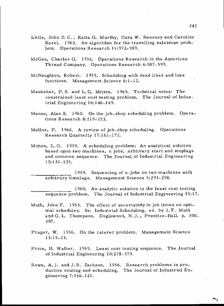
242

Little, John D. C. , Katta G. Murthy, Dura W. Sweeney and Caroline Karel. 1963. An algorithm for the travelling salesman problem. Operations Research 11 :972 -989.

McGee, Charles G. 1956. Operations Research in the American Thread Company. Operations Research 4:587 -599.

McNaughton, Robert. 1959. Scheduling with dead lines and loss functions. Management Science 6:1 -12.

Mankekar, P. S. and L. G. Mitten. 1965. Technical notes: The constrained least cost testing problem. The Journal of Indus- trial Engineering 16:146 -149.

Manne, Alan S. 1960. On the job -shop scheduling problem. Opera- tions Research 8 :219 -223.

Mellor, P. 1966. A review of job -shop scheduling. Operations Research Quarterly 17 :161 -172.

Mitten, L. G. 1959. A scheduling problem: An analytical solution based upon two machines, n jobs, arbitrary start and stoplags and common sequence. The Journal of Industrial Engineering 10 :131_135.

1959. Sequencing of n -jobs on two machines with arbitrary timelags. Management Science 5 :293- 298.

1960. An analytic solution to the least cost testing sequence problem. The Journal of Industrial Engineering 11 :17.

Muth, John F. 1963. The effect of uncertainity in job times on optimal schedules. In: Industrial Scheduling, ed. by J. F. Muth and G. L. Thompson. Englewood, N. J. , Prentice -Hall. p. 300- 3 07.

Prager, W. 1956. On the caterer problem. Management Science 13:15 -23.

Price, H. Walter. 1959. Least cost testing sequence. The Journal of Industrial Engineering 10:278-279.

Rowe, A. J. and J. R. Jackson. 1956. Research problems in production routing and scheduling. The Journal of Industrial En- gineering 7:116-121.

`t

Sasieni, M. , A. Yaspan and L. Friedman. 1959. Operations research - methods and problems. New York, Wiley. 318 p.

Schild, Albert and Irwin J. Fredman. 1961. On scheduling tasks with associated linear loss functions. Management Science 7 :280 -285.

1962. Scheduling tasks with deadlines and non- linear loss functions. Management Science 9:73 -81.

Sisson, Roger L. 1959. Methods of sequencing job- shops: A review. Operations Research 7:10-29_.

243

1961. Sequencing theory. In: Progress in operations research, ed. by Russel L. Ackoff. Vol. 1. New York, Wiley. p. 293 -326. (Operations Research Society of America. Publications in Operations Research no. 5)

Smith, Wayne E. 1956. Various optimizers for single -stage production. Naval Research Logistics Quarterly 3:59 -66.

Story, A. E. and H. M. Wagner. 1963. Computational experience with integer programming for job -shop scheduling. In: Indus- trial scheduling, ed. by J. F. Muth and G. L. Thompson. Englewood Cliffs, N. J. , Prentice -Hall. p. 207 -224.

Vazsonyi, Andrew. 1957. Economic lot size formulas in manufacturing. Operations Research 5: 28 -44.

1958. Scientific programming in business and in- dustry. New York, Wiley. 474 p.

Wagner, Harvey M. 1959. An integer linear programming model for machine scheduling. Naval Research Logistics Quarterly 6 :131 -140.

Wetzel, Wolfgang G. 1957. Comments on, "production scheduling by the transportation method of linear programming. " Opera- tions Research 5 :440 -442.

Optimizers for single and multi-stage job-shop scheduling ...

Documents

Transcript of Optimizers for single and multi-stage job-shop scheduling ...