
BY DR LOIZOS CHRISTOU OPTIMIZATION. Optimization Techniques.

Optimization Techniques for
Data Mining and
Information Reconstruction
Candidate: Gianpiero Bianchi
Supervisor: Renato Bruni
Dissertation submitted in Partial Fulfillment of the
Requirements for the Degree of
Doctor of Philosophy
in
Operations Research
“Sapienza” University of Rome

Contents
Acknowledgments iii
Preface v
1 Introduction to Data Mining and Information Reconstruc-tion 11.1 Generalities of Data Mining . . . . . . . . . . . . . . . . . . . 11.2 Data Mining Tasks . . . . . . . . . . . . . . . . . . . . . . . . 31.3 Overview on Data Mining Classification
Methods . . . . . . . . . . . . . . . . . . . . . . . . . . . . . . 51.4 Information Reconstruction Problems . . . . . . . . . . . . . 81.5 Integer and Mixed Integer Linear Programming Models . . . 111.6 Branch&Bound and Branch&Cut Solution
Techniques . . . . . . . . . . . . . . . . . . . . . . . . . . . . 171.7 Rules based on Propositional Logic . . . . . . . . . . . . . . . 24
2 Classification based on Discretization and MILP 292.1 The Problem of Data Classification . . . . . . . . . . . . . . . 292.2 Classifying with the LAD Methodology . . . . . . . . . . . . 322.3 Evaluation of Binary Attributes . . . . . . . . . . . . . . . . . 372.4 Reformulations of the Support Set Selection Problem . . . . . 422.5 Pattern Generation and Use . . . . . . . . . . . . . . . . . . . 442.6 Implementation and Computational Results . . . . . . . . . . 492.7 Summary and remarks . . . . . . . . . . . . . . . . . . . . . . 56
3 Balancing Problem in Agriculture 573.1 The Problem of Matrix Balancing . . . . . . . . . . . . . . . 573.2 Formulating the MILP Model . . . . . . . . . . . . . . . . . . 593.3 Computational Analysis . . . . . . . . . . . . . . . . . . . . . 643.4 Summary and Remarks . . . . . . . . . . . . . . . . . . . . . 69
i

ii CONTENTS
4 Reconstruction of Cultivation Data in Agriculture 714.1 Reconstruction of Cultivation Data . . . . . . . . . . . . . . . 714.2 A Discrete Mathematical Model . . . . . . . . . . . . . . . . . 724.3 Computational Results . . . . . . . . . . . . . . . . . . . . . . 774.4 Summary and Remarks . . . . . . . . . . . . . . . . . . . . . 79
5 A Formal Procedure for Finding Contradictions into a Setof Rules 815.1 The Problem of Contradictions Localization . . . . . . . . . . 815.2 Encoding Rules into Linear Inequalities . . . . . . . . . . . . 825.3 Locating Contradictions by Means of Linear Programming . 855.4 Applying the Proposed Procedure . . . . . . . . . . . . . . . 905.5 Summary and Remarks . . . . . . . . . . . . . . . . . . . . . 101
References 103
Acknowledgments
I would like to express my sincere gratitude to my supervisor, Renato Bruni,for his constant support, guidance and encouragement. His competence andskill in Operations Research and related fields helped me in solving difficultmathematical questions arising from important practical problems, allowingme to successfully treat very large datasets and to produce a number ofresearch papers.
I also thank the other faculty members of the DIAG Department of the“Sapienza” University of Rome, for their interest in my research work onthe proposed topics.
I am grateful to my colleagues at Istat for their contribution to thedevelopment of Data Editing and Imputation systems and in particular toall the members of the MTO-D operating unit, that was charged to performthe several thousands of runs needed for the treatment of the Census data.
Finally, I take this opportunity to express my deepest gratitude to myfamily for their encouragement and constant support.
iii

iv ACKNOWLEDGMENTS

Preface
Data Mining problems are very important and frequent in several applicativefields. Extracting knowledge from large datasets is a demanding problemthat requires indeed powerful computational resources. However, succeedingin these tasks depends not only on brute computational strength, but also,and often critically, on the mathematical quality of the models and of thealgorithms underlying the solution procedures.
Linear optimization models with integer, binary or continuous variablespossess a high expressive power, and are especially suitable to representseveral Data Mining problems. Continuous variables can be used for exampleto represent a wide variety of real-valued quantities, possibly bounded to benon-negative. Discrete variables, on the other hand, allow the representationof options in the cases where indivisibility is required or where there is nota continuum of solutions, as it happens in many real problems characterizedby a choice.
The presence of discrete variables generally makes the problem more dif-ficult. The finite number of alternatives is in fact not a simplification, withrespect to the case of a continuum of possibilities, because of the impres-sive number of such alternatives in real world problems. However, recentyears have witnessed a huge amount of research in this field, and consequentdecisive algorithmic improvements.
A number of new approaches to classical Data Mining problems arepresented in this thesis. Some of them have been applied to Agriculturaldata, because the author is employed in the Italian National Institute ofStatistics (Istat), in particular in the Census data service, and during theyears of his PhD study the main issue of the service was treating datafrom the Italian Census of Agriculture 2010. This was the occasion forapplying the proposed techniques to very important real-world problems.The contents of this thesis have been presented to some conferences andpublished in international journals.
This work is organized as follows.
v

vi PREFACE
Chapter 1 provides a brief overview of Data Mining and InformationReconstruction. After this, a general introduction to Integer and MixedInteger Linear Programming is reported. Some introductory elements ofPropositional Logic are also given, and the conversion of logical rules intolinear inequalities is explained.
Chapter 2 presents an innovative classification procedure based on dis-cretization and statistical analysis that allow to classify with a good degreeof accuracy and in short times even when the available training sets aresmall. The proposed methodology uses, as much as possible, all the infor-mation extracted from the training set. The problems are formulated asmixed integer linear programming. The procedure has been tested on a testbed of public available datasets from UCI repository. Results are reportedand discussed.
Chapter 3 presents an innovative methodology for solving the problem ofbalancing of Agricultural Census data by using a mixed integer linear model.This mathematical problem is called matrix balancing. The proposed pro-cedure has been applied in the case of the Italian Census of Agriculture 2010to restore data consistency when a total cultivation area, or a total numberof livestock, is not equal to the sum of the detailed values representing theparts of the above totals.
Chapter 4 presents an innovative automatic procedure for assigning thecorrect cultivations to the area for which the farm declarations have beendetected as unreliable. The proposed procedure is based on a discrete math-ematical optimization model. This approach has been applied in the specificcase of vineyard data reconstruction of the mentioned Agricultural Census.
Finally, Chapter 5 presents an innovative automatic procedure for findingcontradictions into a set of rules, that operates by converting those rules intolinear inequalities. The problem is thus converted into a linear programmingproblem. The proposed procedure has been tested in the case of a set ofsimulated rules for economical regulation.
Obviously, the techniques described in Chapters 3 and 4 by referringto agricultural data can be used to solve many other problems of differentorigin but sharing the same logical characteristics.
Roma, Italy, September 2013. Gianpiero Bianchi

Chapter 1
Introduction to Data Miningand InformationReconstruction
1.1 Generalities of Data Mining
Data mining is an interdisciplinary field of computer science, involving meth-ods at the intersection of artificial intelligence, machine learning, statistics,optimization and database systems. The objective of data mining is toidentify previously unknown, potentially useful, and understandable corre-lations and patterns in large datasets. Aside from the raw analysis step, itinvolves database and data management aspects, data preprocessing, modeldevelopment, inference, study of metrics, complexity considerations, post-processing of discovered structures, visualization, updating. Consequently,data mining consists of more than collection and managing data, it alsoincludes analysis and prediction.
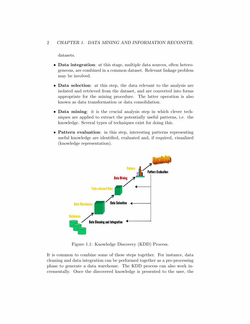
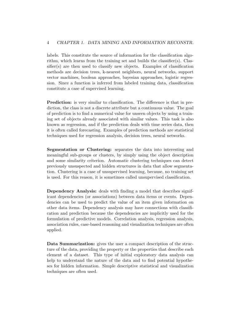
The term Knowledge Discovery in Databases (KDD) is generally used torefer to the overall process of discovering useful knowledge from data, wheredata mining becomes a particular step in this process. Note, however, thatthere are communities in which the whole process in also called data mining.The KDD process consists of the following steps:
• Data cleaning: in this phase, noise and errors in data are removedfrom the dataset, and missing values are imputed. This may in manycases be a difficult problem, a specially in the case of very large
1
2 CHAPTER 1. DATA MINING AND INFORMATION RECONSTR.
datasets.
• Data integration: at this stage, multiple data sources, often hetero-geneous, are combined in a common dataset. Relevant linkage problemmay be involved.
• Data selection: at this step, the data relevant to the analysis areisolated and retrieved from the dataset, and are converted into formsappropriate for the mining procedure. The latter operation is alsoknown as data transformation or data consolidation.
• Data mining: it is the crucial analysis step in which clever tech-niques are applied to extract the potentially useful patterns, i.e. theknowledge. Several types of techniques exist for doing this.
• Pattern evaluation: in this step, interesting patterns representinguseful knowledge are identified, evaluated and, if required, visualized(knowledge representation).
Figure 1.1: Knowledge Discovery (KDD) Process.
It is common to combine some of these steps together. For instance, datacleaning and data integration can be performed together as a pre-processingphase to generate a data warehouse. The KDD process can also work in-crementally. Once the discovered knowledge is presented to the user, the
1.2. DATA MINING TASKS 3
evaluation measures can be enhanced, the mining can be further refined,new data can be selected or further transformed, or new data sources canbe integrated, in order to get different, more appropriate results.
Data mining techniques are nowadays used in several applicative fields, forexample:
• Database Analysis (Extraction of rules, Associations).
• Market Analysis (Customer profiling, Marketing).
• Risk Analysis (Finance planning, Investments).
• Fraud Detection (Credit cards, Food adulteration).
• Decision Support (Resource management, Allocation).
• Medical Analysis (Diagnosis, Management donors).
• Text mining (news group, email, documents) on the Web.
• Economic and Social Policy Analysis (Rule learning).
• Analysis of Rare Events.
1.2 Data Mining Tasks
Several types of data mining problem, or analysis tasks are typically encoun-tered during a data mining project. Depending on the desired outcome, sev-eral data analysis techniques with different goals may be applied successivelyto achieve a desired result. For example, to determine which customers arelikely to buy a new product, a business analyst may need first to use clusteranalysis to segment the customer database, then apply regression analysisto predict buying behavior for each cluster. The data mining tasks typicallyfall into one of the general categories listed below.
Classification: assumes that the objects should be associable with classes,that are the elements of a discrete set of labels. The objective is to buildclassification models, i.e. classifiers, that assign the correct class to pre-viously unseen and unlabeled objects. Classification approaches normallyuse a training set where all objects are already associated with known class
4 CHAPTER 1. DATA MINING AND INFORMATION RECONSTR.
labels. This constitute the source of information for the classification algo-rithm, which learns from the training set and builds the classifier(s). Clas-sifier(s) are then used to classify new objects. Examples of classificationmethods are decision trees, k-nearest neighbors, neural networks, supportvector machines, boolean approaches, bayesian approaches, logistic regres-sion. Since a function is inferred from labeled training data, classificationconstitute a case of supervised learning.
Prediction: is very similar to classification. The difference is that in pre-diction, the class is not a discrete attribute but a continuous value. The goalof prediction is to find a numerical value for unseen objects by using a train-ing set of objects already associated with similar values. This task is alsoknown as regression, and if the prediction deals with time series data, thenit is often called forecasting. Examples of prediction methods are statisticaltechniques used for regression analysis, decision trees, neural networks.
Segmentation or Clustering: separates the data into interesting andmeaningful sub-groups or clusters, by simply using the object descriptionand some similarity criterion. Automatic clustering techniques can detectpreviously unsuspected and hidden structures in data that allow segmenta-tion. Clustering is a case of unsupervised learning, because, no training setis used. For this reason, it is sometimes called unsupervised classification.
Dependency Analysis: deals with finding a model that describes signif-icant dependencies (or associations) between data items or events. Depen-dencies can be used to predict the value of an item given information onother data items. Dependency analysis may have connections with classifi-cation and prediction because the dependencies are implicitly used for theformulation of predictive models. Correlation analysis, regression analysis,association rules, case-based reasoning and visualization techniques are oftenapplied.
Data Summarization: gives the user a compact description of the struc-ture of the data, providing the property or the properties that describe eachelement of a dataset. This type of initial exploratory data analysis canhelp to understand the nature of the data and to find potential hypothe-ses for hidden information. Simple descriptive statistical and visualizationtechniques are often used.
1.3. OVERVIEW ON DATA MINING CLASSIFICATION METHODS 5
1.3 Overview on Data Mining ClassificationMethods
In data mining, classification is one of the most important task, and in thisthesis we will focus on that. As seen, the aim of the classification is tobuild a classifier based on a set of already classified cases (the training set).Then, the classifier is used to predict the class of new cases based on thevalues of their attributes. Commonly used methods for classification can besubdivided into the following groups. Note, however, that the following listis not meant to cover all possible classification techniques, since this taskcould be pursued by using the most heterogeneous approaches.
Decision Trees (DTs): are flowchart-like tree structures, where each inter-nal node denotes a test on an attribute, each branch represents an outcomeof the test, and each leaf node (or terminal node) holds a class label [80].The topmost node in a tree is the root node. During tree construction,attribute selection measures are used to select the attribute which best par-titions the tuples into distinct classes. Three popular attribute selectionmeasures are Information Gain, Gain Ratio, and Gini Index. When DTsare built, many of the branches may reflect noise or outliers in the trainingdata. Tree pruning attempts to identify and remove such branches, with thegoal of improving classification accuracy on unseen data.
k-Nearest Neighbor: is based on learning by analogy, that is by com-paring a given test tuple with training tuples which are similar to it [38].The training tuples are described by n attributes. Each tuple represents apoint in an n-dimensional space. In this way, all of the training tuples arestored in an n-dimensional pattern space. When given an unknown tuple,a k-nearest neighbor (k-NN) classifier searches the pattern space for the ktraining tuples which are closest to the unknown tuple. These k trainingtuples are the k-nearest neighbors of the unknown tuple. “Closeness” isdefined in terms of a distance metric, such as Euclidean distance. The Eu-clidean distance between two points or tuples X1 = (x11, x12, . . . , x1n) andX2 = (x21, x22, . . . , x2n) obtained from the following equation:
dist(X1, X2) =
√√√√ n∑i=1
(x1i − x2i)2 (1.1)
The basic steps of the k-NN algorithm are:
6 CHAPTER 1. DATA MINING AND INFORMATION RECONSTR.
• to compute the distances between the new sample and all previoussamples that have already been classified into clusters;
• to sort the distances in increasing order and select the k samples withthe smallest distance values;
• to apply the voting principle. A new sample will be added (classified)to the largest cluster out of k selected samples [68].
Neural Networks (NN): are those systems modeled based on the humanbrain working citerosenblatt. As the human brain consists of millions ofneurons that are interconnected by synapses, a neural network is a set ofconnected input/output units in which each connection has a weight asso-ciated with it. The network learns in the learning phase by adjusting theweights so as to be able to predict the correct class label of the input. Anartificial neural network consists of connected set of processing units. Theconnections have weights that determine how one unit will affect other. Twosubsets of such units act as input nodes and output nodes, while remainingnodes constitute the hidden layer. By assigning activation to each of theinput node, and allowing them to propagate through the hidden layer nodesto the output nodes, neural network performs a functional mapping frominput values to output values [100].
Support Vector Machine (SVM): attempts to find a linear hyperplaneseparating the different classes. Since very often they are not directly lin-early separable, this technique uses a nonlinear mapping to transform theoriginal training data into a higher dimension. Within this new dimen-sion, it searches for the linear optimal separating hyperplane. A hyperplaneis a “decision boundary” separating the tuples of one class from another.With an appropriate nonlinear mapping to a sufficiently high dimension,data from two classes can always be separated by a hyperplane. The SVMfinds this hyperplane using support vectors (“essential” training tuples) andmargins (defined by the support vectors) [37]. SVM performs classificationtasks by maximizing the margin separating both classes while minimizingthe classification errors.
Logical and boolean approaches: these methodologies aim at extractingor discovering knowledge from data in logical form. The most known booleanapproach is the Logical Analysis of Data (LAD) [18]. The key features of theLAD are the discovery of minimal sets of features necessary for explaining
1.3. OVERVIEW ON DATA MINING CLASSIFICATION METHODS 7
all observations and the detection of hidden patterns in the data capable ofdistinguishing observations describing positive outcome events from negativeoutcome events. Combinations of such patterns are used for developinggeneral classification procedures. LAD methodology is based on discretemathematics, and all data should be encoded into binary form by means ofa process called “binarization”. This process consisting in the replacement ofeach numerical variable by binary indicator variables, each showing whetherthe value of the original variable is present or absent, or is above or belowa certain level. This is done by using the training set for computing specificvalues for each field.
Naıve Bayes: are statistical classifiers. They can predict class membershipprobabilities [101]. Naıve Bayes (NB) probabilistic classifiers are commonlystudied in machine learning. The basic idea in NB approaches is to use thejoint probabilities of words and categories to estimate the probabilities ofcategories given a document. The naıve part of NB methods is the assump-tion of word independence, i.e. the conditional probability of a word given acategory is assumed to be independent from the conditional probabilities ofother words given that category. This assumption makes the computationof the NB classifiers far more efficient than the exponential complexity ofnon-naıve Bayes approaches because it does not use word combinations aspredictors.
Boosting: is a meta-algorithm which can be viewed as a model averagingmethod and belongs to the class of ensemble techniques [86]. We first createa “weak” classifier, such that its accuracy on the training set is only slightlybetter than random guessing. A succession of models are built iteratively,each one being trained on a dataset in which it is assigned more weightto misclassified points by the previous model. Finally, all of the successivemodels are weighted according to their success and then the outputs arecombined using voting thus creating a final model.
Logistic Regression (LR): measures the relationship between a categor-ical dependent variable and one or more independent variables, which areusually (but not necessarily) continuous, by using probability scores as thepredicted values of the dependent variable [77]. Rather than choosing pa-rameters that minimize the sum of squared errors (like in ordinary regres-sion), estimation in logistic regression chooses parameters that maximizethe likelihood of observing the sample values. Frequently LR is used to referspecifically to the problem in which the dependent variable is binary, that
8 CHAPTER 1. DATA MINING AND INFORMATION RECONSTR.
is, the number of available categories is two. LR is being used as a binaryclassification model. To measure the suitability of a binary regression model,one can classify both the actual value and the predicted value of each ob-servation as either 0 or 1 [75]. The predicted value of an observation can beset equal to 1 if the estimated probability that the observation equals 1 isabove 1/2, and set equal to 0 if the estimated probability is below 1/2.
Genetic Algorithms / Evolutionary Programming: are algorithmicoptimization strategies that are inspired by the principles observed in nat-ural evolution [92]. Of a collection of potential problem solutions that com-pete with each other, the best solutions are selected and combined with eachother. In doing so, one expects that the overall goodness of the solution setwill become better and better, similar to the process of evolution of a popu-lation of organisms. Genetic algorithms and evolutionary programming areused in data mining to formulate hypotheses about dependencies betweenvariables, in the form of association rules or some other internal formalism.A disadvantage of Genetic algorithms is that the solutions are difficult toexplain. Also, they do not provide interpretive statistical measures thatenable the user to understand why the procedure arrived at a particularsolution.
Fuzzy Sets: form a key methodology for representing and processing un-certainty [98]. Uncertainty arises in many forms in todays databases: im-precision, non-specificity, inconsistency, vagueness, etc. Fuzzy sets exploituncertainty in an attempt to make system complexity manageable. As such,fuzzy sets constitute a powerful approach to deal not only with incomplete,noisy or imprecise data, but may also be helpful in developing uncertainmodels of the data that provide smarter and smoother performance thantraditional systems. Fuzzy classification is the process of grouping elementsinto a fuzzy set whose membership function is defined by the truth valueof a fuzzy propositional function [102]. A fuzzy propositional function isan expression containing one or more variables, such that, when values areassigned to these variables, the expression becomes a fuzzy proposition inthe sense of [99].
1.4 Information Reconstruction Problems
In the past, for several fields, an automatic information processing has oftenbeen prevented by the scarcity of available data. Nowadays data are veryabundant, but the problem that frequently arises is that such data may
1.4. INFORMATION RECONSTRUCTION PROBLEMS 9
contain errors. This again makes an automatic processing not applicable,since the result is not reliable. Data correctness is indeed a crucial aspect ofdata quality. The relevant problems of error detection and correction shouldtherefore be solved. When dealing with massive datasets, such problems areparticularly difficult to formalize and very computationally demanding tosolve. Since these problems have been studied in different fields of researchthey received different names. While in the field of database managementthey are called data cleaning, in the field of statistics they are called dataediting and imputation, and the correction process is often subdivided intoan error localization phase and a data imputation phase.
As customary for structured information, data are organized into records.The structure of records, called record scheme R, consists in a set of fieldsfi, with i = 1 . . .m. A record instance r, also simply called record, consistsin a set of values vi, one for each field of the scheme.
R = f1, . . . , fm r = v1, . . . , vm (1.2)
Each field fi, with i = 1 . . .m, has its domain Di, which is the set of everypossible value for that field. Since we are dealing with errors, the domainsinclude all values that can be found in data, even the erroneous ones. Arecord instance p is declared correct if and only if it respects a set of rulesdenoted by R = r1, . . . , ru. Each rule can be seen as a mathematical functionrk from the Cartesian product of all the domains to the Boolean set {0,1},as follows.
rk : D1 × · · · ×Dm → {0, 1}p 7→ 0, 1
(1.3)
Rules are such that p is a correct record if and only if rk(p) = 1 for allk = 1 . . . u.
Error Localization The problem of error localization is to find a set H offields of minimum total cost such that a corrected record pc can be obtainedfrom an erroneous record pe by changing (only and all) the values of H.Since H is a subset of the set of all fields {1, . . . ,m}, this problem has acombinatorial optimization structure.
Data Imputation Imputation of actual values of H can then be performedin a deterministic or probabilistic way. This causes the minimum changesto erroneous data, but may have little respect for the original frequencydistributions. A donor record pd is a correct record which should be assimilar as possible to the (unknown) original record po. This is obtained by

10 CHAPTER 1. DATA MINING AND INFORMATION RECONSTR.
selecting pd being as close as possible to pe, according to a suitable functionδ giving a value v called the distance between pe and pd.
δ : (D1 × · · · ×Dm)× (D1 × · · · ×Dm) → IR+
(pe, pd) 7→ v(1.4)
The problem of imputation through a donor is to find a set K of fields ofminimum total cost such that pc can be obtained from pe by copying fromthe donor pd (only and all) the values of K. This is generally recognized tocause low alteration of the original frequency distributions, although changescaused to erroneous data may be not minimum. This is deemed to produce arecord which should be as close as possible to the original record (the recordthat would be present in absence of errors). The correction by means of adonor is also referred to as data driven approach. Because of its relevanceand spread, the above problem has been extensively studied in a variety ofscientific communities. Several different rules encoding and solution algo-rithm have been proposed (e.g. [8, 43, 78, 94]). A very well-known approachto the problem, which implies the generation of all rules logically impliedby the initial set of rules, is due to Fellegi and Holt [47]. In practical case,however, such methods suffer from severe computational limitations [78, 94],with consequent heavy limitations on the number of rules and records thatcan be considered.
Several approaches to data correction problems use mathematical pro-gramming techniques. By requiring to change at least one of the valuesinvolved in each violated rule, a (mainly) set covering model of the errorlocalization problem has been considered by many authors. Such modelhave been solved by means of cutting plane algorithms in [53] for the case ofcategorical data, and in [54, 81] for the case of continuous data. The aboveprocedures has been adapted to the case of a mix of categorical and contin-uous data in [43], were a branch-and-bound approach to the problem is alsoconsidered. Such model, however, does not represent all the problem‘s fea-tures, in the sense that the solution to such model may fail to be a solutionto the localization problem, the separation of the error localization phasefrom the imputation phase may originate artificial restrictions during the lat-ter one, and computational limitations still hold. An automatic procedurefor generic data correction by using a more effective discrete mathematicalmodel of the problem is presented in [24, 26, 27]. This approach overcomesthe computational limits of other techniques (see e.g. [8, 71, 94]), based onthe Fellegi Holt approach, and allows to preserve, as far as it is possible, themarginal and joint distribution within the data.

1.5. INTEGER ANDMIXED INTEGER LINEAR PROGRAMMINGMODELS11
1.5 Integer and Mixed Integer Linear Program-ming Models
Integer and mixed integer programming are subsets of the broader field ofmathematical programming. Mathematical programming formulations usea set of decision variables, which represent actions or decisions that can betaken in the system being modeled. One then attempts to optimize (eitherin the minimization or maximization sense) an objective, that is a functionof these variables which maps each possible set of decisions into a singlescore that assesses the quality of the solution. The limitations of the systemare included as a set of constraints, which are usually stated by restrictingfunctions of the decision variables to be equal to, not more than, or notless than, a certain numerical value. Another type of constraint can simplyrestrict the set of values to which a variable might be assigned.
Several applications involve decisions that are discrete (e.g., to whichhospital an emergency patient should be assigned), while some other de-cisions are continuous in nature (e.g., determining the dosage of fluids tobe administered to a patient). When a problem contains only continuousvariables and linear objective and constraints, the problem is called linearprogramming. When on the contrary a problem contains only discrete vari-ables and linear objective and constraints, the problem is called integer linearprogramming. Note that a parallelism can be traced between integer linearprogramming and combinatorial optimization with linear objective function[76]. When a problem contains both types of variables and linear objectiveand constraints, the problem is called mixed integer linear programming.
While discrete variables may appear easy to handle, the number of com-binations of their values is usually huge, and so complete enumeration tech-niques have important implications on processing time. As the problem sizeincreases, complete enumeration approaches are not computationally viable.Computer speedups, however impressive, are simply no match for exponen-tial enumeration problems. Therefore, more efficient techniques are requiredto solve problems containing discrete variables. Those techniques do not ex-plicitly examine every possible combination of discrete solutions, but insteadexamine a subset of possible solutions, and use optimization theory to provethat no other solution can be better than the best one found. This type oftechnique is referred to as implicit enumeration.

12 CHAPTER 1. DATA MINING AND INFORMATION RECONSTR.
Linear Programming Linear Programming problems (LP, also called“linear programs”) use a set of decision variables, which are the unknownquantities or decisions that are to be optimized. In the context of linearand mixed integer programming problems, the function that assesses thequality of the solution, called the “objective function”, should be a linearfunction of the decision variables. An LP will either minimize or maximizethe value of the objective function. Finally, the decisions that must bemade are subject to certain requirements and restrictions of a system. Weenforce these restrictions by including a set of constraints in the model.Each constraint requires that a linear function of the decision variables iseither equal to, not less than, or not more than, a scalar value. A commoncondition simply states that each decision variable must be nonnegative. Infact, all linear programming problems can be transformed into an equivalentminimization problem with nonnegative variables and equality constraints[9].
A solution that satisfies all constraints is called a feasible solution. Fea-sible solutions that achieve the best objective function value (accordingto whether one is minimizing or maximizing) are called optimal solutions.Sometimes no feasible solution exists, and the optimization problem itselfis called infeasible. On the other hand, some feasible LP problems have nooptimal solution, because it is possible to achieve infinitely good objectivefunction values with feasible solutions. Such problems are called unbounded.
Thus, suppose we denote x1, . . . , xn to be our set of decision variables.Linear programming problems take on the form:
min or max c1x1 + c2x2 + · · ·+ cnxn
subject to a11x1 + a12x2 + · · ·+ a1nxn (≤,=, or ≥) b1a21x1 + a22x2 + · · ·+ a2nxn (≤,=, or ≥) b2. . .am1x1 + am2x2 + · · ·+ amnxn (≤,=, or ≥) bm
xj ≥ 0 ∀j = 1, . . . , n
(1.5)
Values cj ,∀j = 1, . . . , n, are referred to as objective coefficients, and areoften associated with the costs associated with their corresponding deci-sions in minimization problems, or the revenue generated from the corre-sponding decisions in maximization problems. The values b1, . . . , bm arethe right-hand-side values of the constraints, and often represent amountsof available resources (especially for ≤ constraints) or requirements (espe-cially for ≥ constraints). The aij-values thus typically denote how much
1.5. INTEGER AND MIXED INTEGER LINEAR MODELS 13
of resource/requirement i is consumed/satisfied by decision j. Note thatnonlinear terms are not allowed in the model, prohibiting for instance themultiplication of two decision variables, the maximum of several variables,or the absolute value of a variable.
Any maximization (minimization) problem can be converted into a min-imization (maximization) problem by multiplying the coefficients of the ob-jective function by -1.
max
n∑j=1
cjxj = −min
n∑j=1
−cjxj
Moreover, each linear programming problem in generic form can be trans-formed into an equivalent problem in canonical form:
min∑n
j=1 cjxn
subject to∑n
j=1 aijxj ≥ bi ∀i = 1 . . .m
xj ≥ 0 ∀j = 1, . . . , n
(1.6)
This canonical form can be expressed in a compact notation as follows.
min cTxAx ≥ bx ∈ IRn
(1.7)
where x represents the vector of variable (to be determined), c e b are vectorof coefficients, A is a (known) matrix of coefficients. The inequalities Ax ≥ bare constraints which specify a convex politope over which the objectivefunction is to be optimized. Linear programming problems can be convertedinto canonical form as follows:
• For each variable xj , add the equality constraint xj = x+j − x−j and
the inequalities x+j ≥ 0 and x−j ≥ 0.
• Replace any equality constraint∑
j aijxj = bi with two inequalityconstraints
∑j aijxj ≥ bi and
∑j aijxj ≤ bi.
• Replace any constraint∑
j aijxj ≤ bi with the equivalent constraint∑j −aijxj ≥ −bi.

14 CHAPTER 1. DATA MINING AND INFORMATION RECONSTR.
Another useful format for linear programming problems is standard form,which is expressed as:
min cTxsubject to Ax = band x ≥ 0
(1.8)
Note that a LP not in standard form can be converted to standard form byeliminating inequalities by introducing slack and/or surplus variables andreplacing variables that are not sign-constrained with the difference of twosign-constrained variables.
Mixed Integer Linear Programming When some of the variables arerestricted to take integer values, the problem becomes a Mixed Integer Lin-ear Programming one (MILP, also called “mixed integer linear programs”).When variables are restricted to take on either 0 or 1 values the term “in-teger” is replaced with “0-1” or “binary”. All that was specified for thecase of linear programming holds, mutatis mutandis, for the mixed integercase. Typically, modeling MILP requires the definition of a set of decisionvariables, that represent choices that must be optimized in the system, andthe statement of an objective function and constraints (see also [93]).
It is very common, though, to recognize during model construction thatthe initial set of decision variables defined for the model are inadequate. Of-ten, decision variables that seem to be implied consequences of other actionsmust also be defined. The addition of new variables after an unsuccessful at-tempt at formulating constraints and objectives is the “loop” in the process.The correct definition of decision variables can be especially complicated inmodeling with integer variables. If one is allowed to use binary variables ina formulation, it is possible to represent yes-or-no decisions, enforce if-thenstatements, and even permit some sorts of nonlinearity in the model (whichcan be transformed to an equivalent mixed integer linear program).
Some common tips and tricks in modeling with integer variables are:
1. Integrality of quantities. In staffing and purchasing decisions, it is oftenimpossible to take fractional actions. One cannot hire, for instance, 6.5new staff members, or purchase 1.3 hospital beds. The most obvioususe of integer variables thus arises in requesting integer amounts ofquantities that can only be ordered in integer amounts. In general,the optimal solution of an integer program need not be a rounded-offversion of an optimal solution to a linear program.
2. If-then statements. Consider two continuous (i.e., possibly fractional)variables, x and y, defined so that 0 ≤ x ≤ 10 and 0 ≤ y ≤ 10.

1.5. INTEGER AND MIXED INTEGER LINEAR MODELS 15
Suppose we wish to make a statement that if x > 4, then y ≤ 6.On the surface, since no integer quantities are requested, it does notappear that integer variables will be necessary. However, the generalform of linear programs as given in equations (1.5) does not permitif-then statements like the one above. Instead, if-then statements canbe enforced with the aid of a binary variable, z. We wish to makez = 1 if x > 4 (note that we make no claims on z if x ≤ 4). This canbe accomplished by adding the constraint:
x ≤ 4 + 6z (1.9)
since the event that x > 4 implies that z = 1 (even if z = 1, thelargest value for x is 10, which now makes a constraint of the form x is10 unnecessary). If z = 1, then we must also require that y ≤ 6. Thisis achieved by reducing the upper bound of 10 on y to 6 if z is equalto 1 as follows:
y ≤ 10 + 4z (1.10)
where once again, the bound constraint y ≤ 10 may now be omitted.In general, suppose we wish to make the following statement: “if q1x1+· · ·+ qnxn > Q, then r1x1 + · · ·+ rnxn ≤ R”. The following conditionsshould be included in the model:
q1x1 + · · ·+ qnxn ≤ q +M ′z (1.11)
r1x1 + · · ·+ rnxn ≤M ′′ − (M ′′ −R)z (1.12)
z binary (1.13)
where M ′ and M ′′ are “sufficiently large” constants. These valuesshould be just large enough to not add unintentional restrictions tothe model. For instance, we are not attempting to place any hardrestriction on the quantity q1x1 + · · ·+ qnxn (written conveniently asqTx in vector form). If z = 1, the upper bound on qTx is Q + M ′,and hence M ′ must be large enough so that even if constraint (1.11) isremoved from the model, qTx would still never be more than Q+M ′.Likewise, if z = 0, a large enough value of M ′′ must be chosen in(1.12) such that rTx could never be more than M ′′ even without therestriction (1.12). It is worth noting that assigning arbitrarily largevalues for M ′ and M ′′ is not recommended.
3. Enforce at least k out of p restrictions. This situation is similar toif-then constraints in the way we model such restrictions. For a simple
16 CHAPTER 1. DATA MINING AND INFORMATION RECONSTR.
example, suppose we have nonnegative variables x1, . . . , xn, and wishto require that at least three of these variables take on values of 5or more. Then we can define binary variables z1, . . . , zn, such that ifzj = 1, then xj ≥ 5, ∀j = 1, . . . , n. This simple if-then constraint caneasily be modeled by employing the following constraints:
xj ≥ 5zj ∀j = 1, . . . , n (1.14)
Clearly, if zj = 1, then xj ≥ 5. If zj = 0, it is still possible for xj ≥ 5,but no such restrictions are enforced. It is necessary to guaranteethat three variables take on values of 5 or more, and so the following“k-out-of-p” constraint is added:
z1 + · · ·+ zn = 3 (1.15)
Again, this constraint does not state that exactly three variables willbe at least 5, but rather that at least three variables are guaranteedto be at least 5. This same trick can be used to enforce the conditionthat at least k out of p sets of constraints are satisfied, and so on, oftenby using M-values as introduced in the point on if-then constraints.
4. Non linear product terms. In some circumstances, nonlinear termscan be transformed into linear terms by the use of linear constraints.First, note that if xj is a binary variable, then xj = xqj for any positiveconstant q. After that substitution is made, suppose that we have anonlinear term of the form x1 ·x2 · · ·xk ·y, where x1, . . . , xk are binaryvariables and 0 ≤ y ≤ u is another variable, either continuous orinteger. That is, all but perhaps one of the terms is a binary variable.First, replace the nonlinear term with a single continuous variable, w.Using the if-then concept expressed above, note that if xj equals zerofor any j ∈ {1, ..., k}, then w equals zero as well. Also, note that wcan never be more than the upper bound, u, on the y-variable. Hence,we obtain the constraints
w ≤ uxj ∀j = 1, . . . , k (1.16)
Of course, to guarantee that w equals zero in case any xj-variableequals to zero, we must also state a non-negativity constraint:
w ≥ 0 (1.17)
Now, suppose that all x1 = · · · = xk = 1. In this case, it is necessaryto add constraints that enforce the condition that w = y. Regardless

1.6. BRANCH&BOUNDAND BRANCH&CUT SOLUTIONTECHNIQUES 17
of the x-variable values, w cannot be more than y, and so we state theconstraint:
w ≤ y (1.18)
However, in order to get the constraint “w ≥ y if x1 = · · · = xk = 1,”we include the constraint:
w ≥ u(x1 + · · ·+ xk − k) + y (1.19)
If each x-variable equals to 1, then (1.19) states that w ≥ y, whichalong with (1.18) guarantees that w = y. On the other hand, if atleast one xj = 0, j ∈ {1, . . . , k}, then the term u(x1 + · · · + xk − k)is not more than −u, and the right-hand-side of (1.19) is not positive;hence, (1.19) allows w to take on the correct value of zero (as would beenforced by (1.16) and (1.17) ). As a final note, observe that even if yis an integer variable, we need not insist that w is an integer variableas well, since (1.16) - (1.19) guarantee that w = x1 · · ·xk · y, whichmust be an integer given integer x- and y-values.
1.6 Branch&Bound and Branch&Cut SolutionTechniques
Often, there are alternative ways of modeling optimization problems asMILP. There sometimes exist trade-offs in these different modeling ap-proaches. Some models may be smaller (in terms of the number of con-straints and variables required), but may be more difficult to solve thanlarger models. It is important to understand the basics of MILP solutionalgorithms in order to understand the key principles in MILP modeling. Toillustrate the branch-and-bound process, we consider the following exampleMILP:
min 4x1 + 6x2s.t. 2x1 + 2x2 ≥ 5
x1 − x2 ≤ 1x1, x2 ≥ 0 and integer
(1.20)
A relaxation of an MILP is a problem such that (a) any solution to theMILP corresponds to a feasible solution to the relaxed problem, and (b)each solution to the MILP has an objective function value greater than orequal to that of the corresponding solution to the relaxed problem. Themost commonly used relaxation for an MILP is its LP relaxation, which is

18 CHAPTER 1. DATA MINING AND INFORMATION RECONSTR.
identical to the MILP with the exception that variable integrality restrictionsare eliminated. Clearly, any integer-feasible solution to the MILP is also asolution to its LP relaxation, with matching objective function values.
When describing the branch-and-bound algorithm for MILP, it is helpfulto know how LP is solved. See [9, 63, 88, 95] for an explanation of linearprogramming theory and methodology. Graphically, Figure 1.2 illustratesthe feasible region (set of all feasible solutions) to the LP relaxation offormulation (1.20). The point (1.75, 0.75), is the optimal solution to theLP relaxation, and has an objective function value of 11.5. In general, theoptimal solution to the LP is not supposed to be unique, and so it is possiblethat different MILP solutions exist with an identical objective function tothe optimal LP solution. The important result is that a lower bound on theoptimal MILP solution is obtained from the LP relaxation. No solution tothe MILP can be found with an objective function value less than 11.5.
Of course, the solution (1.75, 0.75) is not a feasible solution to (1.20).All feasible solutions have the trait that either x1 ≤ 1 or x1 ≥ 2. In fact,the problem (1.20) can be splitted into two subproblems: one in whichx1 ≤ 1 (called region 1), and one in which x1 ≥ 2 (called region 2). Allsolutions to the original MILP are contained in exactly one of these twonew subproblems. This process is called branching, and we could have alsobranched on x2 instead, by requiring that either x2 ≤ 0 or x2 ≥ 1.
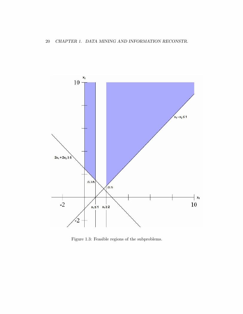
The feasible regions of the two new subproblems are depicted in Fig-ure 1.3. When x1 ≤ 1, the optimal solution is (1, 1.5) with objective func-tion value 13. When x1 ≥ 2, the optimal solution is (2, 1) with objectivefunction value 14. In the x1 ≤ 1 region, the lower bound is 13. In thex1 ≥ 2 region, though, the best solution happens to be an integer solution.Therefore, the best integer solution in the x1 ≥ 2 region has an objectivefunction value of 14; there is no need to further search that region. Thisregion is said to be fathomed by integrality. We store the solution (2, 1),and call it incumbent solution. If no better solution is found, it will becomeour optimal solution.
At this point, there is one active region (or “active node” in the contextof branch-and-bound trees), which is region 1. An active region is one thathas not been branched on, and that must still be explored, because there isa possibility that it contains a solution better than the incumbent solution.The initial region is not active, because we have branched on it. Region 2is not active since the best integer solution has been found in that region.Region 1, however, is still active and must be explored. The lower boundover this region is 13; thus, the optimal solution to the entire problem musthave an objective function value somewhere between 13 and 14 (inclusive).

1.6. B&B AND B&C SOLUTION TECHNIQUES 19
Figure 1.2: Feasible region of the LP relaxation.
20 CHAPTER 1. DATA MINING AND INFORMATION RECONSTR.
Figure 1.3: Feasible regions of the subproblems.
1.6. B&B AND B&C SOLUTION TECHNIQUES 21
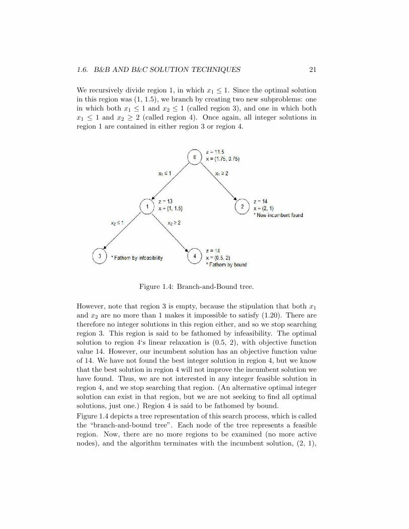
We recursively divide region 1, in which x1 ≤ 1. Since the optimal solutionin this region was (1, 1.5), we branch by creating two new subproblems: onein which both x1 ≤ 1 and x2 ≤ 1 (called region 3), and one in which bothx1 ≤ 1 and x2 ≥ 2 (called region 4). Once again, all integer solutions inregion 1 are contained in either region 3 or region 4.
Figure 1.4: Branch-and-Bound tree.
However, note that region 3 is empty, because the stipulation that both x1and x2 are no more than 1 makes it impossible to satisfy (1.20). There aretherefore no integer solutions in this region either, and so we stop searchingregion 3. This region is said to be fathomed by infeasibility. The optimalsolution to region 4‘s linear relaxation is (0.5, 2), with objective functionvalue 14. However, our incumbent solution has an objective function valueof 14. We have not found the best integer solution in region 4, but we knowthat the best solution in region 4 will not improve the incumbent solution wehave found. Thus, we are not interested in any integer feasible solution inregion 4, and we stop searching that region. (An alternative optimal integersolution can exist in that region, but we are not seeking to find all optimalsolutions, just one.) Region 4 is said to be fathomed by bound.
Figure 1.4 depicts a tree representation of this search process, which is calledthe “branch-and-bound tree”. Each node of the tree represents a feasibleregion. Now, there are no more regions to be examined (no more activenodes), and the algorithm terminates with the incumbent solution, (2, 1),
22 CHAPTER 1. DATA MINING AND INFORMATION RECONSTR.
as an optimal solution.
A formal description of the branch-and-bound algorithm for minimiza-tion problems is given as follows.
Step 0 Set the incumbent objective v = ∞ (assuming that no initialfeasible integer solution is available). Set the active node count k = 1and denote the original problem as an “active” node. Go to Step 1.
Step 1 If k = 0, then stop: the incumbent solution is an optimalsolution. (If there is no incumbent, i.e., v = ∞, then the originalproblem has no integer solution.) Else, if k > 1, go to Step 2.
Step 2 Choose any active node, and call it the “current” node. Solvethe LP relaxation of the current node, and make it inactive. If thereis no feasible solution, then go to Step 3. If the solution to the currentnode has objective value z∗ ≥ v, then go to Step 4. Else, if the solutionis all integer (and z∗ < v), then go to Step 5. Otherwise, go to Step 6.
Step 3 Fathom by infeasibility. Decrease k by 1 and return to Step 1.
Step 4 Fathom by bound. Decrease k by 1 and return to Step 1.
Step 5 Fathom by integrality. Replace the incumbent solution withthe solution to the current node. Set v = z∗, decrease k by 1, andreturn to Step 1.
Step 6 Branch on the current node. Select any variable that is frac-tional in the LP solution to the current node. Denote this variable asxs and denote its value in the optimal solution as f. Create two newactive nodes: one by adding the constraint xs ≤ |f | to the currentnode, and the other by adding xs ≥ |f | to the current node. Add 1 tok (two new active nodes, minus one due to branching on the currentnode) and return to Step 1.
Note that in Step 0, a heuristic procedure could be executed to quickly obtaina good-quality solution to the MILP with no guarantees on its optimality.This solution would then become our initial incumbent solution, and couldpossibly help conserve branch-and-bound memory requirements by increas-ing the rate at which active nodes are fathomed in Step 4. In Step 2, wemay have several choices of active nodes on which to branch, and in Step 6,we may have several choices on which variable to perform the branching op-eration. There has been much empirical research designed to establish good

1.6. B&B AND B&C SOLUTION TECHNIQUES 23
general rules to make these choices, and these rules are implemented in com-mercial solvers. However, for specific types of formulations, one can oftenimprove the efficiency of the branch-and-bound algorithm by experimentingwith node selection and variable branching rules.
The best-case scenario in solving a problem by branch-and-bound is thatthe original node yields an optimal LP solution that happens to be integer,and the algorithm terminates immediately. Indeed, in (1.20), by simplyadding the constraint x1 + x2 ≥ 3 and solve the LP relaxation, we wouldobtain the optimal solution (2, 1) immediately.
Thus, a classical way to reduce the presence of fractional solutions isto find valid inequalities, which do not cut off any integer solutions, butdo cut off some fractional solutions. A cutting plane is a valid inequalitythat removes the optimal LP relaxation solution from the feasible region.The cutting plane method is an umbrella term for optimization methodswhich iteratively refine a feasible set or objective function by means of linearinequalities. Such procedures are generally used to find integer solutions tointeger and mixed integer linear programming problems, and may be usedalso to solve other general optimization problems.
The theory of linear programming dictates that under mild assumptions(if the linear program has an optimal solution, and if the feasible regiondoes not contain a line), one can always find a vertex that is optimal. Theobtained optimal solution is tested for being integer. If it is not, there isguaranteed to exist a linear inequality that separates this LP relaxationsolution from the convex hull of the set of integer solutions. Finding suchan inequality is known as the separation problem, and such an inequality isa cut. A cut can be added to the relaxed linear program. Then, the currentnon-integer solution is no longer feasible to the relaxation. This process isrepeated until an optimal integer solution is found.
In theory, MILP can be solved without branching either by (a) includingenough valid inequalities before solving the LP relaxation, so that the LPrelaxation provides an integer solution, or (b) looping between solving theLP relaxation, adding a cutting plane, and re-solving the LP relaxation,until the LP relaxation yields an integer solution.
However, using these approaches by themselves may suffer from numer-ical instability problems or require the solution of intractable problems.Therefore, the most effective implementations often use a combination ofvalid inequalities added a priori to the model, after which branch-and-boundis executed, with cutting planes periodically added to the nodes of thebranch-and-bound tree. This approach is called “branch-and-cut”. Validinequality and cutting-plane approaches can either be generic or problem-
24 CHAPTER 1. DATA MINING AND INFORMATION RECONSTR.
specific. Clearly, the second approach needs a problem-by-problem analy-sis, but can provide very efficient solution techniques. A large amount ofresearch work on these subjects during the last 50 years lead to the develop-ment of many different cut types. Many classical cutting plane approachesare described in greater detail for instance in [76].
1.7 Rules based on Propositional Logic
Propositional logic, sometimes called sentential logic, may be viewed as agrammar for exploring the construction of complex sentences (propositions)from atomic statements, using the logical connectives. In prepositional logicwe consider formulas (sentences, propositions) that are built up from atomicpropositions that are unanalyzed. In a specific application, the meaning ofthese atomic propositions will be known.
The traditional (symbolic) approach to prepositional logic is based on aclear separation of the syntactical and semantical functions. The syntacticsdeals with the laws that govern the construction of logical formulas fromthe atomic propositions and with the structure of proofs. Semantics, onthe other hand, is concerned with the interpretation and meaning associ-ated with the syntactical objects. Prepositional calculus is based on purelysyntactic and mechanical transformations of formulas leading to inference.
Propositional formulae are syntactically built by using an alphabet overthe two following sets:
• The set of primary logic connectives {¬,∨,∧}, together with the brack-ets () to distinguish start and end of the field of a logic connective.
• The set of proposition symbols, such as x1, x2, . . . , xn.
The only significant sequences of the above symbols are the well-formedformulas (wffs). An inductive definition is the following:
• A propositional symbol x or its negation ¬x.
• Other wffs connected by binary logic connectives and surrounded, incase, by brackets.
Both propositional symbols and negated propositional symbols are calledliterals. Propositional symbols represent atomic (i.e. not divisible) proposi-tions, sometimes called atoms. An example of wff is the following:
(¬x1 ∨ (x1 ∧ x3)) ∧ ((¬(x2 ∧ x1)) ∨ x3) (1.21)

1.7. RULES BASED ON PROPOSITIONAL LOGIC 25
A formula is a wff if and only if there is no conflict in the definition ofthe fields of the connectives. Thus a string of atomic propositions andprimitive connectives, punctuated with parentheses, can be recognized asa well-formed formula by a simple linear-time algorithm. We scan the stringfrom left to right while checking to ensure that the parentheses are nestedand that each field is associated with a single connective. Incidentally, inorder to avoid the use of the awkward abbreviation “wffs”, we will henceforthjust call them propositions or formulas and assume they are well formedunless otherwise noted.
The calculus of propositional logic can be developed using only the threeprimary logic connectives above. However, it is often convenient to permitthe use of certain additional connectives, such as⇒ which is called implies.They are essentially abbreviations that have equivalent formulas using onlythe primary connectives. In fact, if S1 and S2 are formulas, we have:
(S1 ⇒ S2) is equivalent to (¬S1 ∨ S2)
The elements of the set B = {T, F} (or equivalently {1, 0}) are called truthvalues with T denoting True and F denoting False. The truth or falsehoodof a formula is a semantic interpretation that depends on the values of theatomic propositions and the structure of the formula. In order to examinethe above, we need to establish a correspondence between propositionalsymbols and the elements of our Domain. This provides a truth assignment,which is the assignment of values T or F to all the atomic propositions.For this reason, propositions are often, although slightly improperly, calledbinary variables, but no connection with the concept of variable such as inthe case of first-order logic exists.
To evaluate a formula we interpret the logic connectives, with their ap-propriate meaning of “not”, “or”, and “and”. As an illustration, considerthe formula (1.21). Let us start with an assignment of true (T ) for allthree atomic propositions x1, x2, x3. At the next level, of subformulas, wehave ¬x1 evaluates to F , (x1 ∧ x3) evaluates to T , (x2 ∧ x1) evaluates toT , and x3 is T . The third level has (¬x1 ∨ (x1 ∧ x3)) evaluating to T and((¬(x2 ∧ x1)) ∨ x3) also evaluating to T . The entire formula is the “and” oftwo propositions both of which are true, leading to the conclusion that theformula evaluates to T . This process is simply the inductive application ofthe rules:
• S is T if and only if ¬S is F .
• (S1 ∨ S2) is F if and only if both S1 and S2 are F .

26 CHAPTER 1. DATA MINING AND INFORMATION RECONSTR.
• (S1 ∧ S2) is T if and only if both S1 and S2 are T .
The assignment of truth values to atomic propositions and the evaluationof truth/falsehood of formulas is the essence of the semantics of this logic.We now introduce a variety of questions related to the truth or falsehood ofpropositions. The propositional logic uses symbolic valuations of proposi-tions as either True or False. Mathematical programming, however, workswith numerical valuations.
By introducing suitable bounds on the variables, it is possible to restrictvariables to only take values in the nonnegative integers or even just valuesof 0 and 1. This “boolean” restriction captures the semantics of proposi-tional logic since the values of 0 and 1 may be naturally associated withFalse and True. It is natural therefore to express the formulas with clausesrepresented by constraints and atomic propositions represented by 0-1 vari-ables [31]. All the inequality constraints have to be satisfied simultaneously(in conjunction) by any feasible solution.
A positive atom (xi) corresponds to a binary variable (xi), and a negativeatom (¬xi) corresponds to the complement of a binary variable (1 − xi).Consider, for example, the single clause
x2 ∨ ¬x3 ∨ x4
This clause can be converted in the following inequality over (0,1) variables.
x2 + (1− x3) + x4 ≥ 1
Similarly the formula
(x1) ∧ (x2¬x3 ∨ x4) ∧ (¬x1 ∨ ¬x4) ∧ (¬x2 ∨ x3 ∨ x5)
is equivalent to the following system of linear inequalities:
x1 ≥ 1x2 + (1− x3) + x4 ≥ 1(1− x1) + (1− x4) ≥ 1(1− x2) + x3 + x5 ≥ 1
x1, . . . , x5 ∈ {0, 1}
It is conventional in mathematical programming to clear all the constantsto the right-hand side of a constraint. Thus a clause Cj is represented byajx ≥ bj , where for each i, aji is +1 if xi is a positive literal in Cj , is -1 if¬xi is a negative literal in Cj , and is 0 otherwise. Also, bj equals 1−n(Cj),
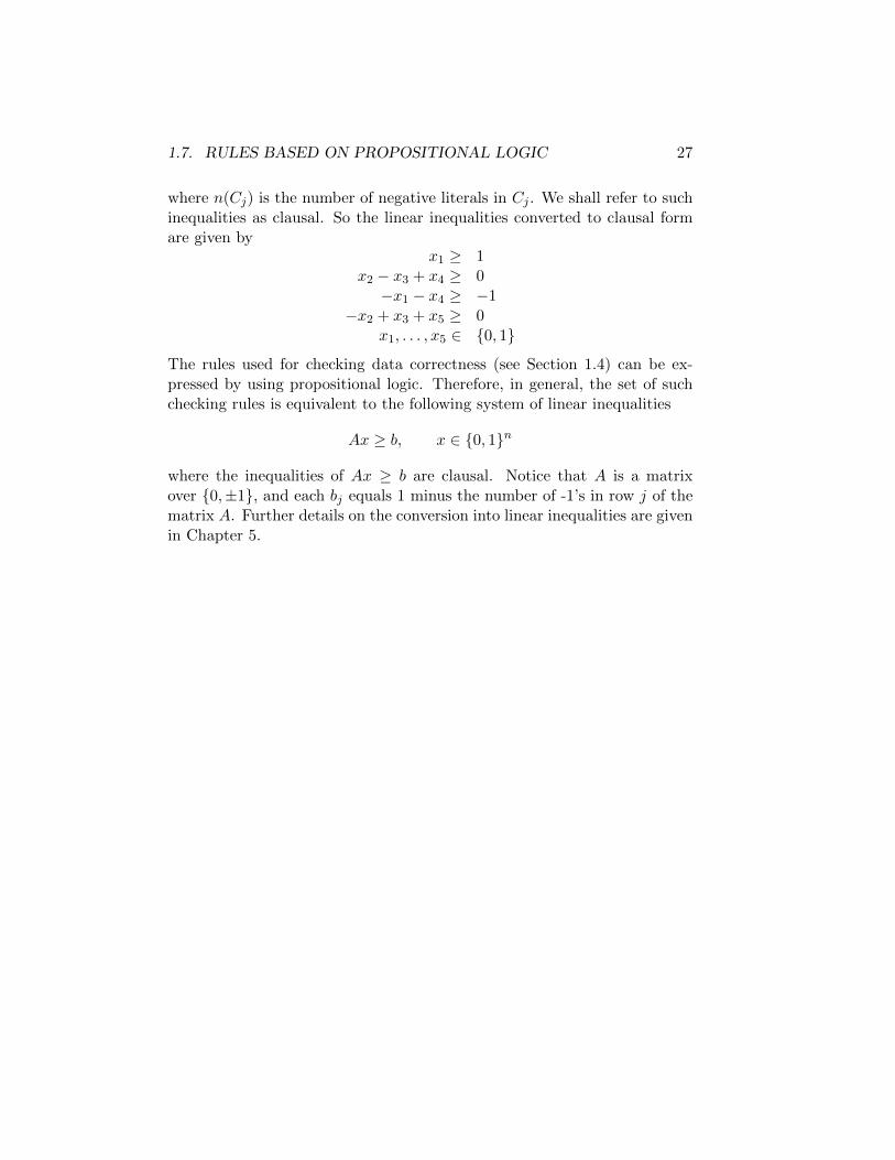
1.7. RULES BASED ON PROPOSITIONAL LOGIC 27
where n(Cj) is the number of negative literals in Cj . We shall refer to suchinequalities as clausal. So the linear inequalities converted to clausal formare given by
x1 ≥ 1x2 − x3 + x4 ≥ 0−x1 − x4 ≥ −1
−x2 + x3 + x5 ≥ 0x1, . . . , x5 ∈ {0, 1}
The rules used for checking data correctness (see Section 1.4) can be ex-pressed by using propositional logic. Therefore, in general, the set of suchchecking rules is equivalent to the following system of linear inequalities
Ax ≥ b, x ∈ {0, 1}n
where the inequalities of Ax ≥ b are clausal. Notice that A is a matrixover {0,±1}, and each bj equals 1 minus the number of -1’s in row j of thematrix A. Further details on the conversion into linear inequalities are givenin Chapter 5.

28 CHAPTER 1. DATA MINING AND INFORMATION RECONSTR.

Chapter 2
Classification based onDiscretization and MILP
2.1 The Problem of Data Classification
Given a set of data grouped into classes, the problem of predicting whichclass new data should receive is called classification problem. The first setof data is called training set, while the set of new data is called test set. In-stances from the training set should have the same structure and the samenature than those of the test set. Classification is of fundamental signifi-cance in the fields of data analysis and data mining, and several importantpractical decision problems are actually classification problems.
Many approaches to this problem have been proposed, based on dif-ferent considerations and data models. Established ones include: NeuralNetworks, Support Vector Machines, k-Nearest Neighbors, Bayesian ap-proaches, Decision Trees, Logistic regression, Boolean approaches (see forreferences [60, 62, 70, 73, 80, 91, 100]). Each approach has several variants,and algorithms can also be designed by mixing approaches. Specific ap-proaches may fit to specific classification contexts, but one approach that isconsidered quite effective for many practical applications are Support Vec-tor Machines (SVM). They are based on finding a separating hyperplanethat maximizes the margin between the extreme training data of oppositeclasses, possibly after a mapping in an higher dimensional space, see also[32, 37]. However, no single algorithm is currently able of providing the bestperformance on all datasets, and this seems to be inevitable [96]. Predictingwhich algorithm will perform best on a specific dataset has become a learn-ing task on its own, belonging to the area called meta-learning [67]. There-
29

30 CHAPTER 2. CLASSIFICATION BASED ON MILP
fore, techniques based on the aggregation of a set of different (and hopefullycomplementary) classifiers have been investigated. They are called ensembletechniques, and they include Boosting [86, 50] and Bagging [22]. Roughlyspeaking, those techniques generate many weak learners and combine theiroutputs in order to obtain a classification that is both accurate and robust.Ensemble techniques based on tree classifiers, such as Random Forest [23],are often able to provide a good performance. A Random Forest, in particu-lar, is a combination of many tree classifiers, each of which grown on a subsetof data randomly sampled independently, and the classification output is acombination (i.e. the mode) of the outputs of the individual trees.
On the other hand, one interesting Boolean approach is the Logical Anal-ysis of Data (LAD), developed since the 1990’s by Hammer et al. (see[18, 19, 21, 29, 40]). It is inspired by the mental processes that a humanbeing applies when learning from examples a classifier. In the LAD method-ology, data should be encoded into binary form by means of a discretiza-tion process called binarization. This is done by using the training set forcomputing specific values for each field, called cut-points in the case of nu-merical fields, that split each field into binary attributes. Discretization isalso adopted in other classification methodologies, such as decision trees,and several ways for selecting cut-points exists, such as entropy based ones(see e.g. [46, 70]). The selected binary attributes, constituting a supportset, are then combined for generating logical rules called patterns. Patternsare used to classify each unclassified record, on the basis of the sign of aweighted sum of the patterns activated by that record. A main feature ofsuch approach is that patterns constitute also a compact description of thedata, i.e. a generally understandable set of rules that describes the clas-sification rationale (see e.g. [39]). LAD methodology is closely related todecision trees and nearest neighbor methods, and constitutes an extensionof those two approaches, as shown in [21].
In this Chapter the following original enhancements to the LAD method-ology are proposed. First, the idea of evaluating the quality of each cut-pointfor numerical fields and of each binary attribute for numerical fields, anda criterion for doing so. Such quality values are computed by using in-formation extracted from the training set, and are taken into account forimproving the selection of the support set. The support set selection cantherefore be modeled as a weighted set covering problem, and also as a binaryknapsack problem (see e.g. [76, 88]). In a related work, Boros et al. [20]consider the problem of finding essential attributes in binary data, whichagain reduces to finding a small support set with a good separation power.They give alternative formulations of such problem and propose three types

2.1. CLASSIFYING WITH SMALL TRAINING SETS 31
of heuristic algorithm for solving them. An analysis of the smallest supportset selection problem within the framework of the probably approximatelycorrect learning theory, and algorithms for its solution, is also in [2].
Moreover, the classification of the test set is not given here simply onthe basis of the sign of the weighted sum of activated patterns, but by com-paring that weighted sum to a suitable classification threshold. Indeed, wepropose to compute both the values of pattern weights and the value ofclassification threshold in order to minimize errors, by solving a mixed in-teger linear programming problem. The objective of minimizing errors ispursued by (i) minimizing classification errors on records of the training setand by (ii) reproducing in the test set the class distribution of the trainingset. Pattern weights and classification threshold are in fact parameters forthe classification procedure, and, in our opinion, this should allow obtainingthe best choice of these parameters for the specific dataset, overcoming theparameter tuning or guessing phase that always represents a difficult andquestionable step. The proposed approach, based on statistical considera-tions on the data, allows to classify with a good degree of accuracy and inshort times even when the available training sets are small as in the case ofrare events and uncontrollable events.
The known LAD procedure is recalled in Section 2.2. In this Chapter,the “standard” procedure, as described in [19], has been mainly considered,although other variants have been investigated in the literature ([58]). Theoriginal contributions of this work begin with Section 2.3, which explainsmotivations and possible criteria for evaluating the quality of cut-points. Inparticular, we derive procedures for dealing with cut-points on continuousfields having normal (Gaussian) distribution, on discrete fields having bino-mial (Bernoulli) distribution, or on general numerical fields having unknowndistribution. This latter approach is used also for qualitative, or categorical,fields. The support set selection problem is then reformulated as weightedset covering and as binary knapsack in Section 2.4. After that, patterns aregenerated, and computation of pattern weights and classification thresholdare described in Section 2.5. Results of the proposed procedure on publiclyavailable datasets of the UCI repository [49] are analyzed and comparedto those of the standard LAD methodology, and also to those of the Sup-port Vector Machines (SVM [37, 32]) methodology in its implementationLIBSVM [33], which is currently deemed to be one of the more effectiveclassifiers, in Section 2.6.

32 CHAPTER 2. CLASSIFICATION BASED ON MILP
2.2 Classifying with the LAD Methodology
Data used for classification are organized in records. The structure ofrecords, called record scheme R, consists in a set of fields fi, with i = 1 . . .m.A record instance r, also simply called record, consists in a set of values vi,one for each field. Fields are essentially of two types: quantitative, or numer-ical, and qualitative, or categorical. A record r is classified if it is assignedto an element of a set of possible classes C. In many cases, C has only twoelements, and we speak of binary classification. This case will be consideredhereinafter. Note, however, that the proposed procedure, mutatis mutandis,could also be used for the case of multiple classes. A positive record instanceis denoted by r+, a negative one by r−.
For classifying, a training set S of classified records is given. Denote byS+ the set of its positive records and by S− the set of its negative ones. SetsS+ and S− constitute our source of information for learning a classifier. Aset of records used for evaluating the performance of the learned classifier iscalled test set T . The real classification of each record t ∈ T should be known.We compare the classification of T given by the learned classifier, also calledpredicted classification, to the real classification of T : the differences are theclassification errors of our classifier. A positive training record is denoted bys+, a negative one by s−. A positive test record is denoted by t+, a negativeone by t−. Very roughly speaking, the larger S is, the more information itcontains, the more accurate our learned classifier will be, even if clearly thereare several aspects involved. However, in many important applications, theavailability of training records is scarce, and a classification methodologyable to be accurate using small training sets would be very useful.
LAD methodology begins with encoding all fields into binary form. Thisprocess, called binarization, converts each (non-binary) field fi into a set ofbinary attributes aji , with j = 1 . . . ni. The total number of binary attributesis n =
∑mi=1 ni. Note that the term “attribute” is not used here as a synonym
of “field”. A binarized record schemeRb is therefore a set of binary attributesaji , and a binarized record instance rb is a set of binary values bji ∈ {0, 1}for those attributes.
Rb = {a11, . . . , an11 , . . . , a
1m, . . . , a
nmm }
rb = {b11, . . . , bn11 , . . . , b
1m, . . . , b
nmm }
For each qualitative fields fi, all values can simply be encoded by means ofa logarithmic number of binary attributes aji , so that ni binary attributescan binarize a quantitative field having up to 2ni different values. For eachnumerical field fi, on the contrary, we introduce ni thresholds called cut-

2.2. CLASSIFYING WITH THE LAD METHODOLOGY 33
points α1i , . . . , α
nii ∈ IR, and the binarization of a value vi is obtained by
considering whether vi lies above or below each αji . Cut-points αji shouldbe set at values representing some kind of watershed, or being otherwiserelevant, for the analyzed phenomenon. Generally, αji are placed in themiddle of specific couples of data values v′i and v′′i :
αji = (v′i + v′′i )/2
This can be done for each couple v′i and v′′i belonging to records from oppositeclasses and adjacent on fi, i.e.:
• v′i ∈ r+ ∈ S+ and v′′i ∈ r− ∈ S−, or vice versa;
• no other training record has a value v′′′i such that v′i < v′′′i < v′′i ifv′i < v′′i , or vice versa if v′′i < v′i.
Cut-points αji are then used for binarizing each numerical field fi into the
binary attributes aji (also called level variables). The values bji of such ajiare
bji =
{1 if vi ≥ αji0 if vi < αji
Note that αji is not required to belong to Di, but only to be comparable, bymeans of ≥ and <, to all values vi ∈ Di.
Example 2.1 Consider the following training set of records representingpersons having fields weight (in Kg.) and height (in cm.), and a positive[respectively negative] classifications meaning “is [resp. is not] a professionalbasketball player”.
weight height pro.bask.player.?
90 195 yes
S+ 100 205 yes
75 180 yes
105 190 noS−
70 175 no
We now plot values belonging to positive [resp. negative] records by using aframed + [resp. −]. Cut-points obtainable from this set S are α1
weight=72.5,
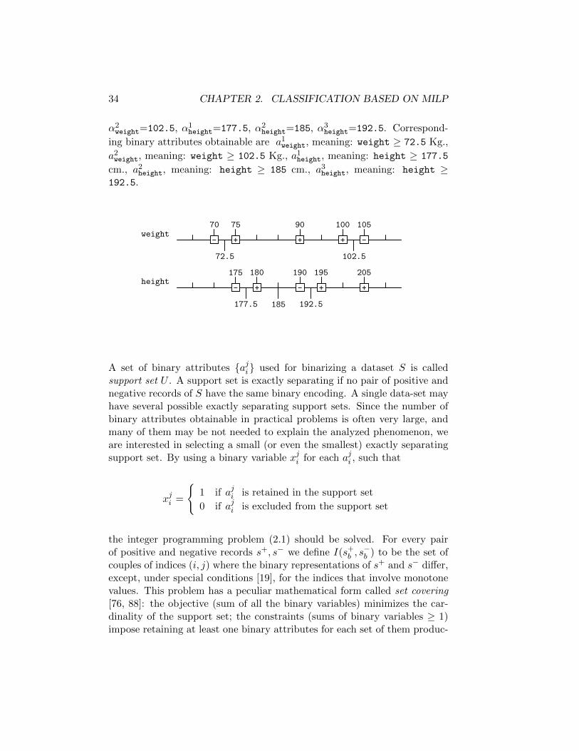
34 CHAPTER 2. CLASSIFICATION BASED ON MILP
α2weight=102.5, α1
height=177.5, α2height=185, α3
height=192.5. Correspond-
ing binary attributes obtainable are a1weight, meaning: weight ≥ 72.5 Kg.,
a2weight, meaning: weight ≥ 102.5 Kg., a1height, meaning: height ≥ 177.5
cm., a2height, meaning: height ≥ 185 cm., a3height, meaning: height ≥192.5.
weight75 90 100 105
72.5 102.5
70
+- + -+
height180 190 195 205
177.5 192.5
175
+- +- +
185
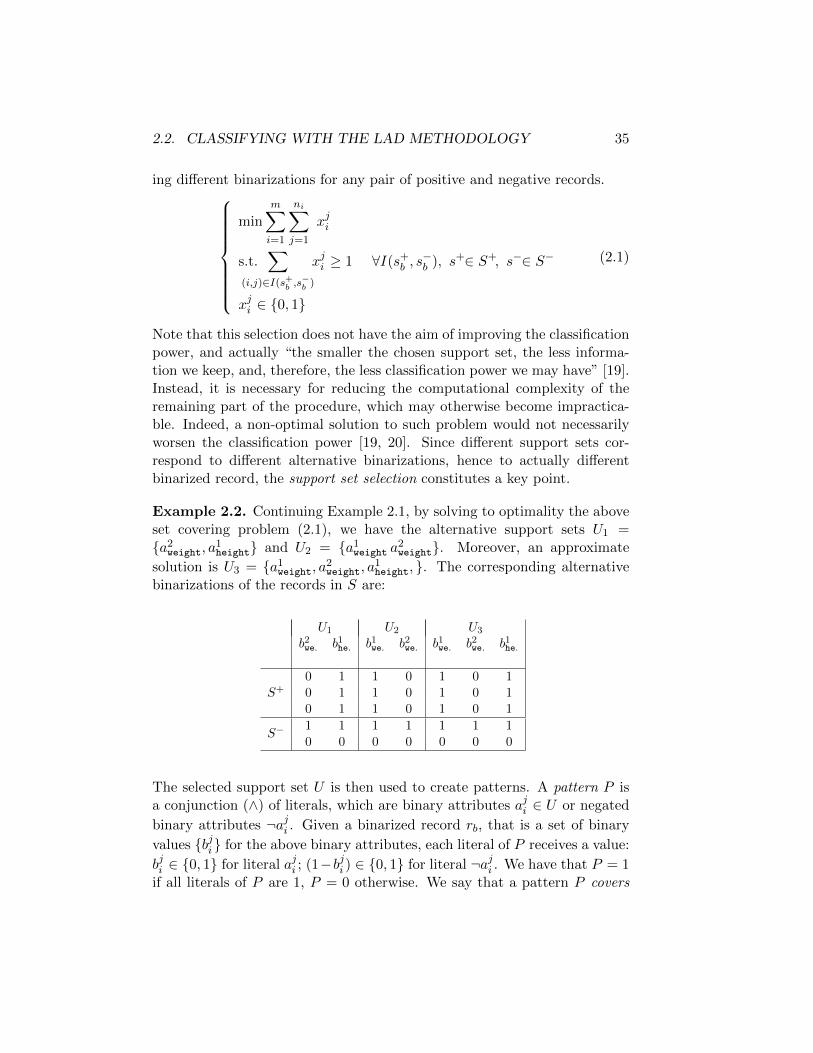
A set of binary attributes {aji} used for binarizing a dataset S is calledsupport set U . A support set is exactly separating if no pair of positive andnegative records of S have the same binary encoding. A single data-set mayhave several possible exactly separating support sets. Since the number ofbinary attributes obtainable in practical problems is often very large, andmany of them may be not needed to explain the analyzed phenomenon, weare interested in selecting a small (or even the smallest) exactly separatingsupport set. By using a binary variable xji for each aji , such that
xji =
{1 if aji is retained in the support set
0 if aji is excluded from the support set
the integer programming problem (2.1) should be solved. For every pairof positive and negative records s+, s− we define I(s+b , s
−b ) to be the set of
couples of indices (i, j) where the binary representations of s+ and s− differ,except, under special conditions [19], for the indices that involve monotonevalues. This problem has a peculiar mathematical form called set covering[76, 88]: the objective (sum of all the binary variables) minimizes the car-dinality of the support set; the constraints (sums of binary variables ≥ 1)impose retaining at least one binary attributes for each set of them produc-
2.2. CLASSIFYING WITH THE LAD METHODOLOGY 35
ing different binarizations for any pair of positive and negative records.
min
m∑i=1
ni∑j=1
xji
s.t.∑
(i,j)∈I(s+b ,s−b )
xji ≥ 1 ∀I(s+b , s−b ), s+∈ S+, s−∈ S−
xji ∈ {0, 1}
(2.1)
Note that this selection does not have the aim of improving the classificationpower, and actually “the smaller the chosen support set, the less informa-tion we keep, and, therefore, the less classification power we may have” [19].Instead, it is necessary for reducing the computational complexity of theremaining part of the procedure, which may otherwise become impractica-ble. Indeed, a non-optimal solution to such problem would not necessarilyworsen the classification power [19, 20]. Since different support sets cor-respond to different alternative binarizations, hence to actually differentbinarized record, the support set selection constitutes a key point.
Example 2.2. Continuing Example 2.1, by solving to optimality the aboveset covering problem (2.1), we have the alternative support sets U1 ={a2weight, a1height} and U2 = {a1weight a2weight}. Moreover, an approximate
solution is U3 = {a1weight, a2weight, a1height, }. The corresponding alternativebinarizations of the records in S are:
U1 U2 U3
b2we. b1he. b1we. b2we. b1we. b2we. b1he.
0 1 1 0 1 0 1S+ 0 1 1 0 1 0 1
0 1 1 0 1 0 1
1 1 1 1 1 1 1S−
0 0 0 0 0 0 0
The selected support set U is then used to create patterns. A pattern P isa conjunction (∧) of literals, which are binary attributes aji ∈ U or negated
binary attributes ¬aji . Given a binarized record rb, that is a set of binary
values {bji} for the above binary attributes, each literal of P receives a value:
bji ∈ {0, 1} for literal aji ; (1−bji ) ∈ {0, 1} for literal ¬aji . We have that P = 1if all literals of P are 1, P = 0 otherwise. We say that a pattern P covers

36 CHAPTER 2. CLASSIFICATION BASED ON MILP
a record r if the set of values rb = {bji} makes P = 1. A positive patternP+ is a pattern covering at least one positive record r+ but no negativeones. A negative pattern P− is defined symmetrically. Patterns admit aninterpretation as rules governing the analyzed phenomenon. We write P (r)for denoting the value of pattern P applied to record r :
P (r) =
{1 if P covers r0 if P does not cover r
Example 2.3. By continuing Example 2.2, a positive pattern obtainedusing the support set U1 is P1 = ¬a2weight ∧ a1height. This means weight <102.5 Kg. and height ≥ 177.5 cm. Recall P1 is a pattern if P1(s
+) = 1for at least some s+ ∈ S and P1(s
−) = 0 for all s− ∈ S. Indeed, we haveP1(s
+) = 1 for all s+ ∈ S and P1(s−) = 0 for all s− ∈ S. Another pattern,
obtained using support set U3, is P2 = a1weight∧¬a2weight∧a1height. P2 appearsto be even more appropriate than P1, since it means “one is a professionalbasketball player if has a medium weight (weight ≥ 72.5 Kg. and weight
< 102.5 Kg.) and height above a certain value (height ≥ 177.5 cm.)”.P2(s
+) = 1 for all s+ ∈ S and P2(s−) = 0 for all s− ∈ S.
Positive patterns can be generated by means of two types of approaches:top-down, i.e. by removing one by one literals from the conjunction of lit-erals covering a single positive record until no negative records are covered,or bottom-up, i.e. by conjoining one by one single literals until obtaining aconjunction covering only positive records. Negative patterns can be gen-erated symmetrically. Also the number of generated patterns may be toolarge, so a pattern selection step can be performed. This is done in [19] bysolving another set covering problem, whose solution gives the set of the in-dices H+ of selected positive patterns and that of the indices H− of selectednegative patterns, with H = H+ ∪ H−. Weights wh are now assigned toall patterns in H, with wh ≥ 0 for h ∈ H+ and wh ≤ 0 for h ∈ H−, byusing criteria described in [19]. We skip detail here since we will discuss thisagain and propose a new approach in Section 2.5. Finally, each new recordr is classified according to the positive or negative value of the followingweighted sum, called discriminant and denoted by ∆(r).
∆(r) =∑h∈H+
whPh(r) +∑h∈H−
whPh(r) =∑h∈H
whPh(r)
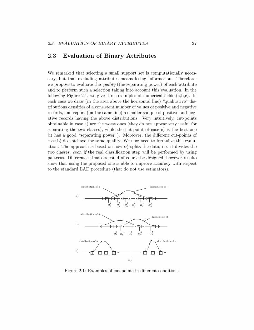
2.3. EVALUATION OF BINARY ATTRIBUTES 37
2.3 Evaluation of Binary Attributes
We remarked that selecting a small support set is computationally neces-sary, but that excluding attributes means losing information. Therefore,we propose to evaluate the quality (the separating power) of each attributeand to perform such a selection taking into account this evaluation. In thefollowing Figure 2.1, we give three examples of numerical fields (a,b,c). Ineach case we draw (in the area above the horizontal line) “qualitative” dis-tributions densities of a consistent number of values of positive and negativerecords, and report (on the same line) a smaller sample of positive and neg-ative records having the above distributions. Very intuitively, cut-pointsobtainable in case a) are the worst ones (they do not appear very useful forseparating the two classes), while the cut-point of case c) is the best one(it has a good “separating power”). Moreover, the different cut-points ofcase b) do not have the same quality. We now need to formalize this evalu-ation. The approach is based on how αji splits the data, i.e. it divides thetwo classes, even if the real classification step will be performed by usingpatterns. Different estimators could of course be designed, however resultsshow that using the proposed one is able to improve accuracy with respectto the standard LAD procedure (that do not use estimators).
a)-+ +
c)++ -
b)+
distribution of + distribution of -
distribution of +
distribution of +
distribution of -
distribution of -
1
aα
3
aα
5
aα
4
aα
6
aα
2
aα
1
bα
2
bα
3
bα
1
cα
4
bα
5
bα
+ - - +
++ --
+ --+-+
Figure 2.1: Examples of cut-points in different conditions.

38 CHAPTER 2. CLASSIFICATION BASED ON MILP
Given a single cut-point αji and a record r, denote by + the fact that ris actually positive, and by − the opposite situation. Moreover, denote byclass + (αji ) the fact that r is classified as positive by αji , i.e. stays on the
positive side of cut-point αji , and by class − (αji ) the fact that r is in theopposite situation. Given a generic set of records N , let A+ be the set ofthe records which are class + (αji ), and A− be the set of records which are
class − (αji ). Denote instead by N+ and N− the (possibly unknown) realpositive and negative sets. Errors occur when a negative record is classifiedas positive, and vice versa. The first kind of errors, called false positive, areN− ∩A+; the second kind of errors, called false negative, are N+ ∩A−. Theconfusion matrix is given in Table 2.1 below.
Real+ −
+ N+ ∩A+ N− ∩A+Predicted by αji − N+ ∩A− N− ∩A−
Table 2.1: Confusion matrix.
Since the described support set selection problem is a non-trivial decisionproblem, it seems reasonable to model it as a binary linear programmingproblem. For doing so, we need to use a criterion for evaluating the qualityof each binary attribute such that the overall quality value of a set of binaryattributes can be given by the sum of their individual quality values. Weobtain this as follows. A basic measure of the accuracy of the positiveclassification obtained from αji can be the probability of producing a truepositive divided by the probability of producing a false positive.
o+(αji ) =Pr(+ ∩ class + (αji ))
Pr(− ∩ class + (αji ))
A similar measure can evaluate the accuracy of the negative classificationobtained from αji .
o−(αji ) =Pr(− ∩ class − (αji ))
Pr(+ ∩ class − (αji ))
Clearly, o+(αji ) ∈ [0,+∞) and o−(αji ) ∈ [0,+∞). The higher the value, the
better positive [resp. negative] classification αji provides. In order to have
a complete evaluation of αji , we consider the product o+(αji ) × o−(αji ) ∈[0,+∞).
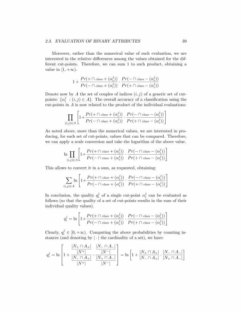
2.3. EVALUATION OF BINARY ATTRIBUTES 39
Moreover, rather than the numerical value of such evaluation, we areinterested in the relative differences among the values obtained for the dif-ferent cut-points. Therefore, we can sum 1 to such product, obtaining avalue in [1,+∞).
1 +Pr(+ ∩ class + (αji ))
Pr(− ∩ class + (αji ))·Pr(− ∩ class − (αji ))
Pr(+ ∩ class − (αji ))
Denote now by A the set of couples of indices (i, j) of a generic set of cut-points: {αji : (i, j) ∈ A}. The overall accuracy of a classification using thecut-points in A is now related to the product of the individual evaluations:
∏(i,j)∈A
[1+
Pr(+ ∩ class + (αji ))
Pr(− ∩ class + (αji ))·Pr(− ∩ class − (αji ))
Pr(+ ∩ class − (αji ))
]
As noted above, more than the numerical values, we are interested in pro-ducing, for each set of cut-points, values that can be compared. Therefore,we can apply a scale conversion and take the logarithm of the above value.
ln∏
(i,j)∈A
[1+
Pr(+ ∩ class + (αji ))
Pr(− ∩ class + (αji ))·Pr(− ∩ class − (αji ))
Pr(+ ∩ class − (αji ))
]
This allows to convert it in a sum, as requested, obtaining:
∑(i,j)∈A
ln
[1+
Pr(+ ∩ class + (αji ))
Pr(− ∩ class + (αji ))·Pr(− ∩ class − (αji ))
Pr(+ ∩ class − (αji ))
]
In conclusion, the quality qji of a single cut-point αji can be evaluated asfollows (so that the quality of a set of cut-points results in the sum of theirindividual quality values).
qji = ln
[1+
Pr(+ ∩ class + (αji ))
Pr(− ∩ class + (αji ))·Pr(− ∩ class − (αji ))
Pr(+ ∩ class − (αji ))
]
Clearly, qji ∈ [0,+∞). Computing the above probabilities by counting in-stances (and denoting by | · | the cardinality of a set), we have:
qji = ln
1 +
|N+ ∩A+||N+|
|N− ∩A+||N+|
·
|N− ∩A−||N−|
|N+ ∩A−||N−|
= ln
[1 +|N+ ∩A+||N− ∩A+|
· |N− ∩A−||N+ ∩A−|
]

40 CHAPTER 2. CLASSIFICATION BASED ON MILP
However, this evaluation needs the correct classification {N+, N−} of thedataset N . We obviously prefer an a priori quality evaluation, i.e. com-putable by knowing only the correct classification of the training set S. Wecan do this by using a non-parametric method for fields having unknowndistribution, and a parametric one for fields having known distribution.
In the case of fields having unknown distribution, qji is simply obtainedby considering the training set S instead of the generic N , while for eachcut-point αji sets A+ and A− are clearly known (they respectively are the
sets or records that are class +(αji ) and class−(αji )). Now, the quality of each
attribute aji over a numerical field fi is that of its corresponding cut-point
αji , that is the defined qji .In the case of fields where the hypothesis of a known distribution is
satisfactory, their positive and negative density functions can be computedusing the training set S, and the above quantities |N+ ∩ A+|, etc. can beevaluated by using such density functions. In other words, we just knowdata from the training set S, but we may infer where other data will be,and compute how useful αji would be for all of them. In particular, for anycontinuous-valued field fi, we make the hypothesis of a normal (Gaussian)distribution. Such distribution can indeed model the majority of real-worldvalues, as a consequence of the central limit theorem [48]. Denote nowby mi+ the mean value that positive records have for fi and by σi+ their
(population) standard deviation (defined as
√∑s∈S+ (vsi−mi+)2
|S+| ), denote by
mi− and σi− the same quantities for the negative records, and supposew.l.o.g. that cut-point αji represents a transition from − to +. By computing
the above parameters from the training set S, our evaluation of quality qjibecomes:
qji = ln
1 +
+∞∫αji
1√2π(σi+)2
e− (t−mi+)2
2(σi+)2 dt
+∞∫αji
1√2π(σi−)2
e− (t−mi−)2
2(σi−)2 dt
·
αji∫−∞
1√2π(σi−)2
e− (t−mi−)2
2(σi−)2 dt
αji∫−∞
1√2π(σi+)2
e− (t−mi+)2
2(σi+)2 dt
In case of a discrete-valued field fi, on the contrary, we make the hypothe-sis of binomial (Bernoulli) distribution. This should indeed describe manydiscrete real-world quantities [48]. Denote now by mi+ and Mi+ the min-imum and the maximum values on field i for positive records, and by mi−and Mi− the same quantities for the negative records. Denote also by

2.3. EVALUATION OF BINARY ATTRIBUTES 41
ni+ = Mi+ −mi+ the number of possible positive values for fi, and by p+the characteristic positive probability of success (also called Bernoulli proba-bility parameter, estimated as |S+|/ni+). Denote by ni− = Mi− −mi− andby p− the same quantities for negative records. Suppose, again, that αji isa transition from − to +. By computing the above parameters from S, ourevaluation of quality qji becomes now:
qji = ln
1+
ni+∑t=αji−mi+
(ni+t
)(pi+)t(1− pi+)ni+−t
ni+∑t=αji−mi+
(ni−t
)(pi−)t(1− pi−)ni−−t
·
αji−mi−−1∑t=0
(ni−t
)(pi−)t(1− pi−)ni−−t
αji−mi−−1∑t=0
(ni+t
)(pi+)t(1− pi+)ni+−t
Moreover, we modify the above qji in order to reduce possible overfittingand to avoid selecting attributes in an unbalanced manner (e.g. all from thesame fields).
We penalize each attribute aji corresponding to a cut-point αji originatedby a few isolated points of one class laying near many points of the oppositeclass. More precisely, we set two thresholds ν1 and ν2 and put qji := qji /2
for each aji such that: i) a number of training records ≤ ν1 lie on one side
of αji , and ii) a number of training records ≥ ν2 (of the opposite class) lie
on the other side of αji .
We also penalize the binary attributes over a field fi from which otherbinary attributes have already been selected. Clearly, this can be appliedonly during a sequential solution (see Section 2.4) of the support set selectionproblem. More precisely, each time an attribute from fi is selected, we putqji := qji /2 for each still unselected attributes of fi.
Note, finally, that for fields having a considerable overlapping betweenthe two classes, cut-points cannot be generated when inverting the class,because almost every region of the field contains both classes. On the con-trary, they are generated when inverting the class predominance, i.e. whenpassing from a region with positive predominance to one with negative pre-dominance and vice versa. By considering the fraction of negative records
in the training |S−||S| , a region has positive predominance when its percentage
of negative records is ≤ g |S−||S| %. Values for g was set at 70.

42 CHAPTER 2. CLASSIFICATION BASED ON MILP
2.4 Reformulations of the Support Set SelectionProblem
When the quality value of each attribute have been computed, the exactlyseparating support set selection problem can be modeled as follows. Wewould like minimizing a weighted sum (and not only the number) of se-lected attributes, where the weights are the reciprocal 1/qji of the quality
qji , while selecting at least an attribute for each of the above defined sets
I(r+b , r−b ). Note that 1/qji can be viewed as a measure of the uselessness
of aji . By using the binary variables xji already introduced in Section 2.2,the following weighted set covering problem should be solved, using the non-negative weights 1/qji .
minm∑i=1
ni∑j=1
1
qjixji
s.t.∑
(i,j)∈I(r+b ,r−b )
xji ≥ 1 ∀I(s+b , s−b ), s+∈ S+, s−∈ S−
xji ∈ {0, 1}
(2.2)
This formulation takes now into account the individual qualities of the at-tributes. One may observe that this would discard attributes that havea poor isolated effect but may have important effect when combined withother attributes during the pattern generation step. However, a selectionis necessary for the computational viability of the entire procedure, andthe proposed approach aims at discarding the attributes that appear moresuitable to be discarded.
Moreover, such weighted set covering formulation (2.2) has strong com-putational advantages on a non-weighted one (2.1). Although still NP-hard[76], solution algorithms become considerably faster when the model vari-ables receive different weight coefficients in the objective function. Depend-ing on the size of the model and on available computational time, suchweighted set covering problem may be either solved to optimality or bysearching for an approximate solution. In the former case, it is guaranteedthat the pattern generation step is performed by using a set of attributesU which is a minimal set for which no positive and negative records havethe same binary encoding. In the latter case, if the approximate solution isfeasible but non-optimal, it is not guaranteed that U is minimal, i.e. it mayexist also a proper subset U ′ ⊂ U such that no positive and negative recordshave the same binary encoding. This could have the effect of increasing the
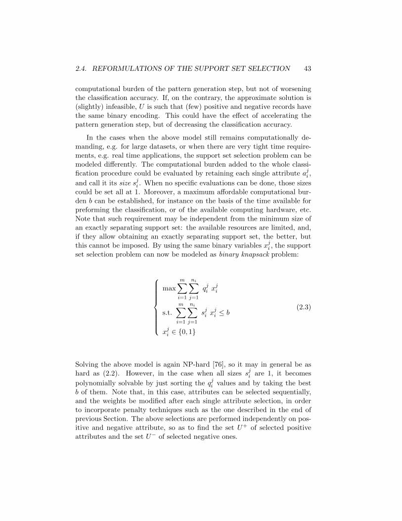
2.4. REFORMULATIONS OF THE SUPPORT SET SELECTION 43
computational burden of the pattern generation step, but not of worseningthe classification accuracy. If, on the contrary, the approximate solution is(slightly) infeasible, U is such that (few) positive and negative records havethe same binary encoding. This could have the effect of accelerating thepattern generation step, but of decreasing the classification accuracy.
In the cases when the above model still remains computationally de-manding, e.g. for large datasets, or when there are very tight time require-ments, e.g. real time applications, the support set selection problem can bemodeled differently. The computational burden added to the whole classi-fication procedure could be evaluated by retaining each single attribute aji ,
and call it its size sji . When no specific evaluations can be done, those sizescould be set all at 1. Moreover, a maximum affordable computational bur-den b can be established, for instance on the basis of the time available forpreforming the classification, or of the available computing hardware, etc.Note that such requirement may be independent from the minimum size ofan exactly separating support set: the available resources are limited, and,if they allow obtaining an exactly separating support set, the better, butthis cannot be imposed. By using the same binary variables xji , the supportset selection problem can now be modeled as binary knapsack problem:
max
m∑i=1
ni∑j=1
qji xji
s.t.
m∑i=1
ni∑j=1
sji xji ≤ b
xji ∈ {0, 1}
(2.3)
Solving the above model is again NP-hard [76], so it may in general be ashard as (2.2). However, in the case when all sizes sji are 1, it becomes
polynomially solvable by just sorting the qji values and by taking the bestb of them. Note that, in this case, attributes can be selected sequentially,and the weights be modified after each single attribute selection, in orderto incorporate penalty techniques such as the one described in the end ofprevious Section. The above selections are performed independently on pos-itive and negative attribute, so as to find the set U+ of selected positiveattributes and the set U− of selected negative ones.
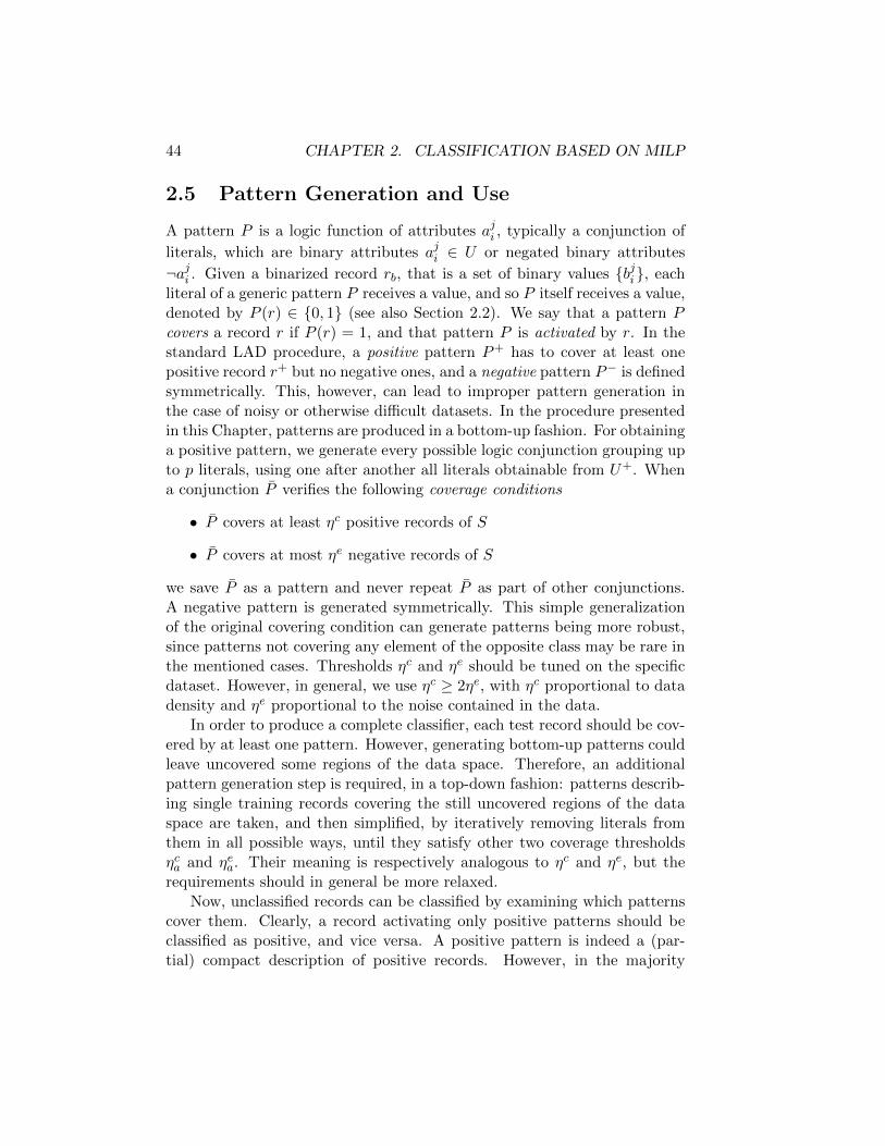
44 CHAPTER 2. CLASSIFICATION BASED ON MILP
2.5 Pattern Generation and Use
A pattern P is a logic function of attributes aji , typically a conjunction of
literals, which are binary attributes aji ∈ U or negated binary attributes
¬aji . Given a binarized record rb, that is a set of binary values {bji}, eachliteral of a generic pattern P receives a value, and so P itself receives a value,denoted by P (r) ∈ {0, 1} (see also Section 2.2). We say that a pattern Pcovers a record r if P (r) = 1, and that pattern P is activated by r. In thestandard LAD procedure, a positive pattern P+ has to cover at least onepositive record r+ but no negative ones, and a negative pattern P− is definedsymmetrically. This, however, can lead to improper pattern generation inthe case of noisy or otherwise difficult datasets. In the procedure presentedin this Chapter, patterns are produced in a bottom-up fashion. For obtaininga positive pattern, we generate every possible logic conjunction grouping upto p literals, using one after another all literals obtainable from U+. Whena conjunction P verifies the following coverage conditions
• P covers at least ηc positive records of S
• P covers at most ηe negative records of S
we save P as a pattern and never repeat P as part of other conjunctions.A negative pattern is generated symmetrically. This simple generalizationof the original covering condition can generate patterns being more robust,since patterns not covering any element of the opposite class may be rare inthe mentioned cases. Thresholds ηc and ηe should be tuned on the specificdataset. However, in general, we use ηc ≥ 2ηe, with ηc proportional to datadensity and ηe proportional to the noise contained in the data.
In order to produce a complete classifier, each test record should be cov-ered by at least one pattern. However, generating bottom-up patterns couldleave uncovered some regions of the data space. Therefore, an additionalpattern generation step is required, in a top-down fashion: patterns describ-ing single training records covering the still uncovered regions of the dataspace are taken, and then simplified, by iteratively removing literals fromthem in all possible ways, until they satisfy other two coverage thresholdsηca and ηea. Their meaning is respectively analogous to ηc and ηe, but therequirements should in general be more relaxed.
Now, unclassified records can be classified by examining which patternscover them. Clearly, a record activating only positive patterns should beclassified as positive, and vice versa. A positive pattern is indeed a (par-tial) compact description of positive records. However, in the majority
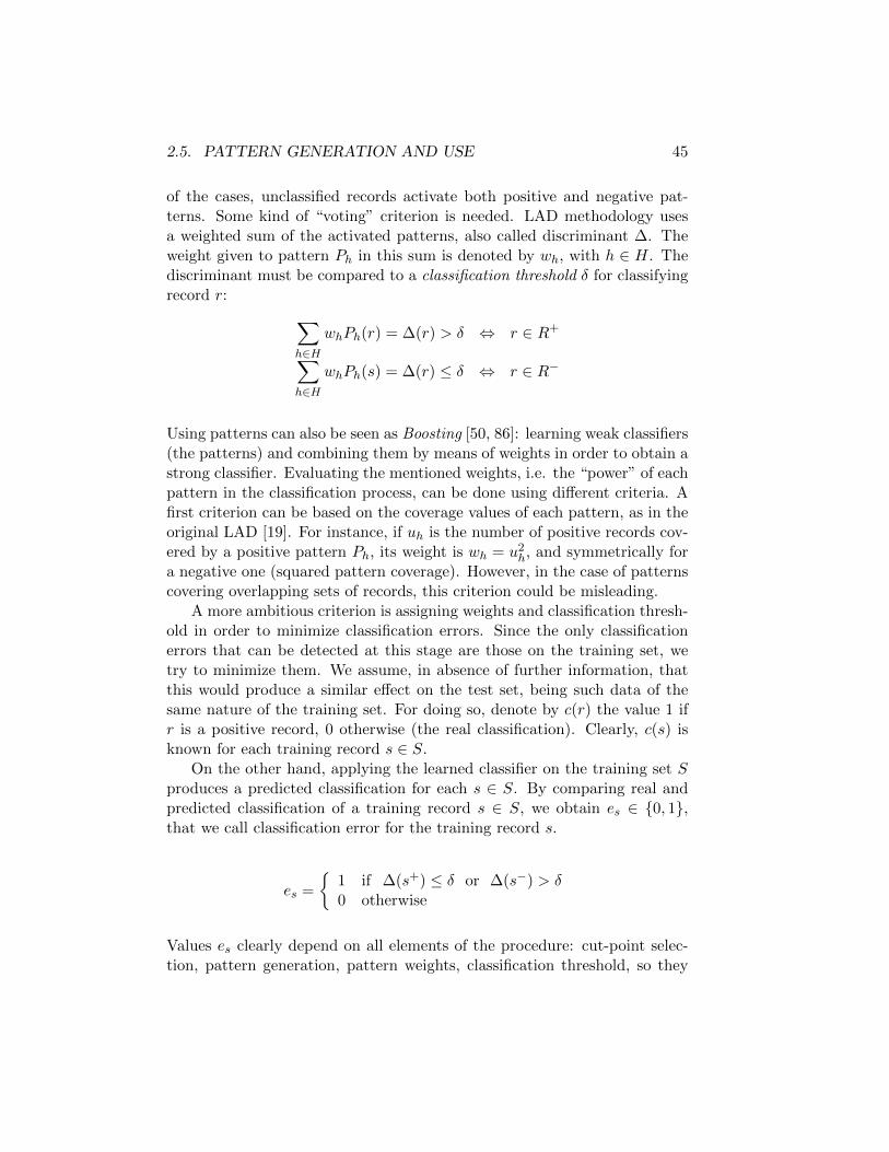
2.5. PATTERN GENERATION AND USE 45
of the cases, unclassified records activate both positive and negative pat-terns. Some kind of “voting” criterion is needed. LAD methodology usesa weighted sum of the activated patterns, also called discriminant ∆. Theweight given to pattern Ph in this sum is denoted by wh, with h ∈ H. Thediscriminant must be compared to a classification threshold δ for classifyingrecord r: ∑
h∈HwhPh(r) = ∆(r) > δ ⇔ r ∈ R+
∑h∈H
whPh(s) = ∆(r) ≤ δ ⇔ r ∈ R−
Using patterns can also be seen as Boosting [50, 86]: learning weak classifiers(the patterns) and combining them by means of weights in order to obtain astrong classifier. Evaluating the mentioned weights, i.e. the “power” of eachpattern in the classification process, can be done using different criteria. Afirst criterion can be based on the coverage values of each pattern, as in theoriginal LAD [19]. For instance, if uh is the number of positive records cov-ered by a positive pattern Ph, its weight is wh = u2h, and symmetrically fora negative one (squared pattern coverage). However, in the case of patternscovering overlapping sets of records, this criterion could be misleading.
A more ambitious criterion is assigning weights and classification thresh-old in order to minimize classification errors. Since the only classificationerrors that can be detected at this stage are those on the training set, wetry to minimize them. We assume, in absence of further information, thatthis would produce a similar effect on the test set, being such data of thesame nature of the training set. For doing so, denote by c(r) the value 1 ifr is a positive record, 0 otherwise (the real classification). Clearly, c(s) isknown for each training record s ∈ S.
On the other hand, applying the learned classifier on the training set Sproduces a predicted classification for each s ∈ S. By comparing real andpredicted classification of a training record s ∈ S, we obtain es ∈ {0, 1},that we call classification error for the training record s.
es =
{1 if ∆(s+) ≤ δ or ∆(s−) > δ0 otherwise
Values es clearly depend on all elements of the procedure: cut-point selec-tion, pattern generation, pattern weights, classification threshold, so they

46 CHAPTER 2. CLASSIFICATION BASED ON MILP
are not easily expressible. However, when knowing whether each patternPh, with h ∈ H, covers or not each record s ∈ S, the above es are simplefunctions of pattern weights {wh} and classification threshold δ. There-fore, given the set of generated pattern {Ph}, we compute the coveragesPh(s) ∈ {0, 1} for all h ∈ H and s ∈ S, obtaining a |H| × |S| matrix PShaving binary elements dhs:
PS = [dhs] with dhs = Ph(s)
The same can be done for each pattern Ph, with h ∈ H and each test recordt ∈ T , obtaining a |H| × |T | matrix PT having binary elements dht:
PT = [dht] with dht = Ph(t)
On the other hand, for each test record t ∈ T , we only know (at this stage)the classification given by the learned classifier, which is again function of{wh} and δ.
ct =
{1 if
∑h∈H whPh(r) > δ
0 if∑
h∈H whPh(r) ≤ δ
Moreover, we want to learn from the training set the class distribution, that
is the fraction of positive |S+||S| (or of negative |S
−||S| ) records contained in
the training set (clearly, given one of the two, the other is also fixed). Wetherefore introduce a value, called tolerance and denoted by γ, measuringthe “difference” from the class distribution of the training set and that ofthe test set. Hence, we have a bi-objective: minimizing the number oferrors on the training set and minimizing the tolerance γ. By introducing ascalarization parameter G > 0, our objective becomes:
min∑s∈S
es +Gγ
A reasonable choice for G is |S|/10, so that the second term of the objectivecannot override the first one (whose theoretical maximum is |S|, but withtypical values between 0.01|S| and 0.4|S|). The description of constraints isfollowing.
2.5. PATTERN GENERATION AND USE 47
We need to impose that the classification error es is 1 for each record s ∈ Ssuch that the classification that s would receive using {wh} and δ does notmatch its real class c(s).
∑h∈H
whdhs − δ ≤M(c(s) + es) ∀s ∈ S (2.4)∑h∈H
whdhs − δ > −M(1− c(s) + es) ∀s ∈ S (2.5)
M is a positive constant greater than any possible value of the first mem-ber (see also [93]). The mathematical behavior of those constraints is thefollowing. When
∑h∈H whdhs − δ > 0, record s is predicted positive. In
this case, the second member of (2.4) must be ≥ than a positive number, soit must be positive, while the second member of (2.5) must be < than thesame positive number, so it can be either 0 or negative: if c(s) = 0 (= theprediction is an error), es is forced to be 1 by the (2.4), while it is free forthe (2.5); if c(s) = 1 (= the prediction is not an error), es is free for bothconstraints.
On the other hand, when∑
h∈H whdhs − δ ≤ 0, record s is predictednegative. In this case, the second member of (2.4) must be ≥ than a number≤ 0, so it can be either 0 or positive, while the second member of (2.5) mustbe < than the same number, so it must be negative: if c(s) = 1 (= theprediction is an error), es is forced to be 1 by the (2.5), while it is free forthe (2.4); if c(s) = 0 (= the prediction is not an error), es is free for bothconstraints. Note that, when es is free for both constraints, the minimizationof the objective will make it 0. In order to have a closed feasible region, (2.5)is converted into ≥ by introducing a small ε > 0
∑h∈H
whdhs − δ ≥ −M(1− c(s) + es) + ε ∀s ∈ S
In order to evaluate the class distribution that {wh} and δ would producein T , we need to compute the predicted classification of its records. Wetherefore need constraints connecting values {wh} and δ to the class ct thatwould be predicted for each record t ∈ T . The machinery is similar to thatof the above analyzed constraints, but note that we do not use at all thereal class of the test records, that must obviously remain unknown during

48 CHAPTER 2. CLASSIFICATION BASED ON MILP
classification process.
∑h∈H
whdht − δ ≤Mct ∀t ∈ T (2.6)∑h∈H
whdht − δ > −M(1− ct) ∀t ∈ T (2.7)
Constraint (2.7) is converted into ≥ by using again a small ε > 0
∑h∈H
whdht − δ ≥ −M(1− ct) + ε ∀t ∈ T
Finally, we need constraints imposing that {wh} and δ reproduce in T the
class distribution of S, so |T+| should be as similar as possible to |S+| · |T ||S|
,
and connecting the difference to the introduced γ.
∑t∈T
ct ≤∑s∈S
c(s) · |T ||S|
+ |T |γ + ρ (2.8)
∑t∈T
ct ≥∑s∈S
c(s) · |T ||S|− |T |γ − ρ (2.9)
Note that, when we need to classify just one or a few records, obtaining thesame class distribution of S could be impossible. For example, if we need
to classify two records, and the fraction of positive |S+||S| is 0.2, targeting at
that class distribution for the two records is clearly useless. Hence, (2.8-2.9) should have no effect when T is very small. This is obtained by usingvalue ρ, that, when set for instance at 3, relaxes constraints (2.8-2.9) of 3units. For large |T | this relaxation is negligible (so it is not considered inthe tests of Section 2.6), while for small |T | the problem gradually reducesto minimizing only the classification error on S.
The overall mixed integer linear model for finding optimal pattern weightswh and classification threshold δ is now the following. Weight values arebounded by a value W , in order to avoid giving excessive importance to anysingle pattern, since that could be a source of overfitting.
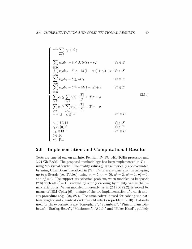
2.6. IMPLEMENTATION AND COMPUTATIONAL RESULTS 49
min∑s∈S
es +Gγ
∑h∈H
whdhs − δ ≤M(c(s) + es) ∀s ∈ S∑h∈H
whdhs − δ ≥ −M(1− c(s) + es) + ε ∀s ∈ S∑h∈H
whdht − δ ≤Mct ∀t ∈ T∑h∈H
whdht − δ ≥ −M(1− ct) + ε ∀t ∈ T∑t∈T
ct ≤∑s∈S
c(s) · |T ||S|
+ |T |γ + ρ∑t∈T
ct ≥∑s∈S
c(s) · |T ||S|− |T |γ − ρ
−W ≤ wh ≤W ∀h ∈ H
es ∈ {0, 1} ∀s ∈ Sct ∈ {0, 1} ∀t ∈ Twh ∈ IR ∀h ∈ Hδ ∈ IRγ ∈ IR+
(2.10)
2.6 Implementation and Computational Results
Tests are carried out on an Intel Pentium IV PC with 3GHz processor and3.24 Gb RAM. The proposed methodology has been implemented in C++using MS Visual Studio. The quality values qji are numerically approximatedby using C functions described in [79]. Pattern are generated by groupingup to p literals (see Tables), using ν1 = 5, ν2 = 50, ηc = 2, ηe = 1, ηca = 1,and ηea = 0. The support set selection problem, when modeled as knapsack(2.3) with all sji = 1, is solved by simply ordering by quality values the bi-nary attributes. When modeled differently, as in (2.1) or (2.2), is solved bymeans of IBM Cplex [65], a state-of-the-art implementation of branch-and-cut procedure (e.g. [76, 88]). The same solver is used for solving the pat-tern weights and classification threshold selection problem (2.10). Datasetsused for the experiments are “Ionosphere”, “Spambase”, “Pima Indians Dia-betes”, “Statlog Heart”, “Mushroom”, “Adult” and “Poker Hand”, publicly
50 CHAPTER 2. CLASSIFICATION BASED ON MILP
available from the UCI Repository of machine learning problems [49]. Theywere chosen in order to have a test bed containing different types of datasets(with many or few records, many or few fields, numerical or categorical, easyor difficult, etc.), so as to analyze the classifiers behavior under all condi-tions.
The first set, Ionosphere, is composed by 351 instances, each having 34fields (plus the class). In particular, there are 32 real-valued fields and 2binary ones. All 32 real-valued fields could be considered having normal dis-tribution, one binary field could be considered having binomial distribution,the other is always 0. They are “data collected by a radar system in GooseBay, Labrador. The targets were free electrons in the ionosphere. Goodradar returns are those showing evidence of some type of structure in theionosphere. Bad returns are those that do not; their signals pass throughthe ionosphere”, from UCI Repository [49].
The second set, Spambase, is composed by 4,601 instances, each having57 fields (plus the class), all numerical. In particular, 55 are real-valuedand 2 are integer; however they are the frequencies of “particular wordsor characters” and numbers of capital letters in an email, so all 57 wereconsidered having normal distribution. Records of this dataset correspondto received emails, and the class “denotes whether the e-mail was consideredspam (1) or not (0), i.e. unsolicited commercial e-mail”, from the UCIRepository [49].
The third set, Pima Indians Diabetes, is composed by 768 instances, eachhaving 8 fields (plus the class). In particular, there are 2 real-valued fieldsand 6 integer ones. However, since 3 integer fields have a number of possiblevalues high enough, 5 field could be considered having normal distribution,while 3 could be considered having binomial distribution. Fields are medicalinformations about “females patients of Pima Indian heritage living nearPhoenix, Arizona, the class is whether the patient shows signs of diabetes”,from the UCI Repository [49].
The forth set, Statlog Heart, is composed by 270 instances, each having13 fields (plus the class). In particular, there are 7 real-valued fields and 6categorical or binary. The first 7 were considered having normal distribution.The last 6 could not be considered having binomial distribution, so they weretreated as those with normal distribution but generating cut-points wheninverting the class predominance due to the few number of possible values(see Section 2.3). Fields are several medical informations about patients,the class is whether the patient “has absence or presence of heart disease”,from the UCI Repository [49].
The fifth set, Mushroom, is composed by 8,124 instances, each having
2.6. IMPLEMENTATION AND COMPUTATIONAL RESULTS 51
22 fields (plus the class). All fields are categorical with very few possi-ble values (no more than 12, some are just 2), so they were treated asthose with binomial distribution but generating cut-points when invertingthe class predominance (see Section 2.3). The records correspond to “mush-rooms described in terms of physical characteristics, from Audobon SocietyField Guide”, and the “classification is poisonous or edible”, from the UCIRepository [49].
The sixth set, Adult, is composed by 48,842 instances, each having 14fields (plus the class). In particular, there are 6 real-valued fields that couldbe considered having normal distribution, the other 8 are categorical andwere treated as fields with unknown distribution. They are “a set of rea-sonably clean person records extracted from the 1994 US Census database”,from the UCI Repository [49]. The class is whether that person earns morethan 50,000 USD per year or not.
The seventh set, Poker Hand, is composed by 1,025,010 instances, eachhaving 10 fields (plus the class). For this dataset, the training set is pre-defined and composed by 25,010 records, corresponding to 2.44% of thetotal. Records have 5 categorical and 5 integer fields, but such integer fieldsshould be considered categorical, since they are values of cards: just labels.All fields were treated as fields with unknown distribution, but the first 5 didnot produce any cut-points, so they were excluded also for LIBSVM in oderto make the classifiers work in the same conditions (note that including themwould produce worse results for LIBSVM). Each record is suit and rank ofthe 5 cards received in the poker game, drawn from a standard deck of 52.The class is the ranking of the entire poker hand, from 0 to 9. In order toobtain a binary classification problem, we assigned 0 to “nothing in hand”and 1 to any other point (pair, two pairs, etc.). The above data-sets havebeen classified using the following procedures:
1. The proposed one, called SLAD (Statistical and Logical Analysis ofData), solving the knapsack version (2.3) of the Support set selection prob-lem and the described Pattern weights and classification threshold selectionproblem (2.10).
2. The standard LAD (Logical Analysis of Data) procedure, obtainedfrom the former by not assigning values to binary attributes and solvingan unweighted set covering problem (2.1) for the Support set selection, andusing pattern weights wh based on squared pattern coverage (see Section2.5) and classification threshold δ = 0.
3. A simplified version of SLAD, called RLAD (Reduced Logical Analy-sis of Data), solving the knapsack version (2.3) of the Support set selectionproblem and simply using the binary attributes for performing the classifi-
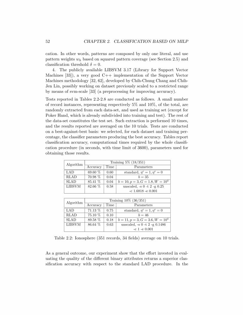
52 CHAPTER 2. CLASSIFICATION BASED ON MILP
cation. In other words, patterns are composed by only one literal, and usepattern weights wh based on squared pattern coverage (see Section 2.5) andclassification threshold δ = 0.
4. The publicly available LIBSVM 3.17 (Library for Support VectorMachines [33]), a very good C++ implementation of the Support VectorMachines methodology [32, 62], developed by Chih-Chung Chang and Chih-Jen Lin, possibly working on dataset previously scaled to a restricted rangeby means of svm-scale [33] (a preprocessing for improving accuracy).
Tests reported in Tables 2.2-2.8 are conducted as follows. A small numberof record instances, representing respectively 5% and 10%, of the total, arerandomly extracted from each data-set, and used as training set (except forPoker Hand, which is already subdivided into training and test). The rest ofthe data-set constitutes the test set. Such extraction is performed 10 times,and the results reported are averaged on the 10 trials. Tests are conductedon a best-against-best basis: we selected, for each dataset and training per-centage, the classifier parameters producing the best accuracy. Tables reportclassification accuracy, computational times required by the whole classifi-cation procedure (in seconds, with time limit of 3600), parameters used forobtaining those results.
AlgorithmTraining 5% (18/351)
Accuracy Time Parameters
LAD 69.60 % 0.60 standard, ηc = 1, ηe = 0
RLAD 70.98 % 0.04 b = 35
SLAD 85.41 % 0.04 b = 10, p = 3, G = 1.8,W = 104
LIBSVM 82.66 % 0.58 unscaled, -s 0 -t 2 -g 0.25-c 1.6818 -e 0.001
AlgorithmTraining 10% (36/351)
Accuracy Time Parameters
LAD 71.13 % 0.75 standard, ηc = 1, ηe = 0
RLAD 75.10 % 0.10 b = 46
SLAD 89.58 % 0.18 b = 11, p = 3, G = 3.6,W = 104
LIBSVM 86.64 % 0.63 unscaled, -s 0 -t 2 -g 0.1486-c 1 -e 0.001
Table 2.2: Ionosphere (351 records, 34 fields) average on 10 trials.
As a general outcome, our experiment show that the effort invested in eval-uating the quality of the different binary attributes returns a superior clas-sification accuracy with respect to the standard LAD procedure. In the

2.6. IMPLEMENTATION AND COMPUTATIONAL RESULTS 53
AlgorithmTraining 5% (230/4601)
Accuracy Time Parameters
LAD 83.10 % 2.14 standard, ηc = 1, ηe = 0
RLAD 75.70 % 0.18 b = 240
SLAD 88.90 % 0.92 b = 100, p = 3, G = 23,W = 104
LIBSVM 85.74 % 1.05 scaled, -s 0 -t 2 -g 0.5-c 8.0 -e 0.001
AlgorithmTraining 10% (460/4601)
Accuracy Time Parameters
LAD 84.32 % 2.21 standard, ηc = 1, ηe = 0
RLAD 78.55 % 0.50 b = 370
SLAD 89.51 % 1.61 b = 200, p = 3, G = 46,W = 104
LIBSVM 89.12 % 1.36 scaled, -s 0 -t 2 -g 0.5-c 8.0 -e 0.001
Table 2.3: Spambase (4601 records, 57 fields) average on 10 trials.
AlgorithmTraining 5% (38/768)
Accuracy Time Parameters
LAD 70.48 % 0.88 standard, ηc = 1, ηe = 0
RLAD 66.10 % 0.03 b = 60
SLAD 72.77 % 0.40 b = 60, p = 3, G = 3.8,W = 104
LIBSVM 70.54 % 0.80 scaled, -s 0 -t 2 -g 0.000173-c 4096 -e 0.001
AlgorithmTraining 10% (76/768)
Accuracy Time Parameters
LAD 72.36 % 1.15 standard, ηc = 1, ηe = 0
RLAD 67.90 % 0.06 b = 64
SLAD 73.96 % 0.62 b = 64, p = 3, G = 7.6,W = 104
LIBSVM 72.38 % 2.84 scaled, -s 0 -t 2 -g 0.25-c 11.31 -e 0.001
Table 2.4: Pima Indians Diabetes (768 records, 8 fields) average on 10 trials.
totality of the analyzed cases, indeed, SLAD is more accurate than LAD.That additional effort clearly required an additional computational time, butthat was almost negligible, and moreover, in the solution of the support setselection problem, weighted set covering problems can generally be solvedin times which are much shorter than those needed for the correspondingnon-weighted ones, so performing the above quality evaluation appears in

54 CHAPTER 2. CLASSIFICATION BASED ON MILP
AlgorithmTraining 5% (14/270)
Accuracy Time Parameters
LAD 62.40 % 0.78 standard, ηc = 1, ηe = 0
RLAD 64.25 % 0.02 b = 54
SLAD 77.23 % 0.02 b = 14, p = 4, G = 1.4,W = 104
LIBSVM 76.44 % 0.20 scaled, -s 0 -t 2 -g 0.00035-c 512 -e 0.001
AlgorithmTraining 10% (27/270)
Accuracy Time Parameters
LAD 68.80 % 0.78 standard, ηc = 1, ηe = 0
RLAD 69.00 % 0.04 b = 64
SLAD 80.24 % 0.04 b = 22, p = 4, G = 2.7,W = 104
LIBSVM 77.52 % 0.34 scaled, -s 0 -t 2 -g 0.125-c 512 -e 0.001
Table 2.5: Statlog Heart (270 records, 13 fields) average on 10 trials.
AlgorithmTraining 5% (406/8124)
Accuracy Time Parameters
LAD 76.90 % 2.67 standard, ηc = 1, ηe = 0
RLAD 76.39 % 0.32 b = 176
SLAD 98.79 % 0.69 b = 20, p = 4, G = 40,W = 104
LIBSVM 98.34 % 1.12 unscaled, -s 0 -t 2 -g 0.03125-c 8.0 -e 0.001
AlgorithmTraining 10% (812/8124)
Accuracy Time Parameters
LAD 80.15 % 3.85 standard, ηc = 1, ηe = 0
RLAD 78.48 % 0.45 b = 200
SLAD 99.72 % 0.83 b = 25, p = 4, G = 81,W = 104
LIBSVM 99.13 % 1.25 unscaled, -s 0 -t 2 -g 0.03125-c 8.0 -e 0.001
Table 2.6: Mushroom (8124 records, 22 fields) average on 10 trials.
any case convenient. Furthermore, the solution of the support set selectionproblem as binary knapsack (2.3) using the above quality evaluation and allsji = 1 is even faster and produces a very good classification accuracy.
The comparison with LIBSVM, which is currently deemed to be one of themost effective classifiers, show the effectiveness of the proposed approach.Indeed, SLAD obtains a classification accuracy that is always comparable
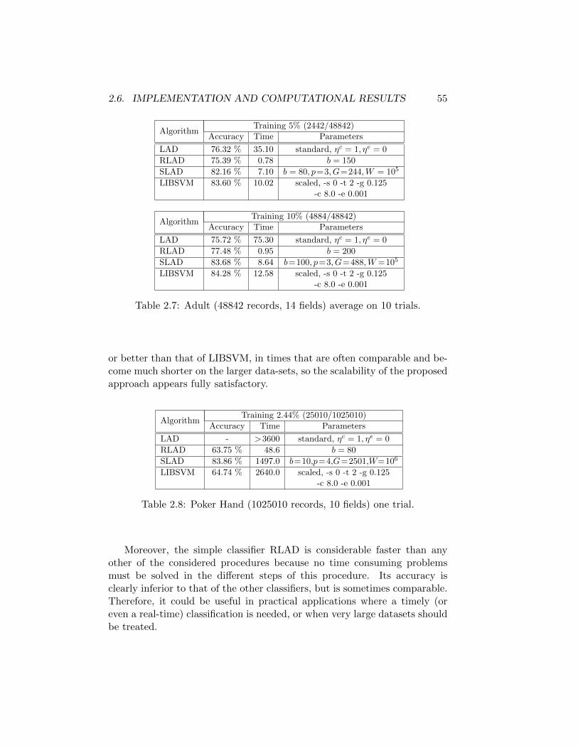
2.6. IMPLEMENTATION AND COMPUTATIONAL RESULTS 55
AlgorithmTraining 5% (2442/48842)
Accuracy Time Parameters
LAD 76.32 % 35.10 standard, ηc = 1, ηe = 0
RLAD 75.39 % 0.78 b = 150
SLAD 82.16 % 7.10 b = 80, p=3, G=244,W = 105
LIBSVM 83.60 % 10.02 scaled, -s 0 -t 2 -g 0.125-c 8.0 -e 0.001
AlgorithmTraining 10% (4884/48842)
Accuracy Time Parameters
LAD 75.72 % 75.30 standard, ηc = 1, ηe = 0
RLAD 77.48 % 0.95 b = 200
SLAD 83.68 % 8.64 b=100, p=3, G=488,W =105
LIBSVM 84.28 % 12.58 scaled, -s 0 -t 2 -g 0.125-c 8.0 -e 0.001
Table 2.7: Adult (48842 records, 14 fields) average on 10 trials.
or better than that of LIBSVM, in times that are often comparable and be-come much shorter on the larger data-sets, so the scalability of the proposedapproach appears fully satisfactory.
AlgorithmTraining 2.44% (25010/1025010)
Accuracy Time Parameters
LAD - >3600 standard, ηc = 1, ηe = 0
RLAD 63.75 % 48.6 b = 80
SLAD 83.86 % 1497.0 b=10,p=4,G=2501,W=106
LIBSVM 64.74 % 2640.0 scaled, -s 0 -t 2 -g 0.125-c 8.0 -e 0.001
Table 2.8: Poker Hand (1025010 records, 10 fields) one trial.
Moreover, the simple classifier RLAD is considerable faster than anyother of the considered procedures because no time consuming problemsmust be solved in the different steps of this procedure. Its accuracy isclearly inferior to that of the other classifiers, but is sometimes comparable.Therefore, it could be useful in practical applications where a timely (oreven a real-time) classification is needed, or when very large datasets shouldbe treated.

56 CHAPTER 2. CLASSIFICATION BASED ON MILP
2.7 Summary and remarks
Classify with a good degree of accuracy and in short times on the basis ofsmall training sets is required in a variety of practical applications. Un-fortunately, obtaining these three desirable features together can be verydifficult. We consider here the framework of the Logical Analysis of Data(LAD), and propose several enhancements to this methodology based on sta-tistical considerations on the data. In particular, we use more informationextracted from the training set to guide the support set selection step, andpropose two reformulations of such a problem having several advantages.Moreover, we consider the problem of selecting the best parameters for theprocedure (pattern weights and classification threshold), and formulate it asan optimization problem, overcoming this way the parameter tuning step.The proposed methodology, called Statistical and Logical Analysis of Data(SLAD), is tested on a test bed of publicly available datasets from the UCIrepository, and compared to the standard LAD methodology and to theSupport Vector Machines (SVM) methodology. Experiments show that thepresented enhancements are able to increase the classification accuracy andreduce computation times with respect to standard LAD methodology. Thecomparison with SVM methodology, currently deemed one of the best classi-fication technique, proves that SLAD provides good accuracy and timing re-sults using very small training sets. Moreover, a simplified version of SLAD,called Reduced Logical Analysis of Data (RLAD), is proposed. All steps ofthis latter procedure can be solved in very short times, allowing a sensiblespeed-up of the whole classification procedure. As a consequence, real-timeclassification, or fast classification of massive datasets, can be undertaken.

Chapter 3
Balancing Problem inAgriculture
3.1 The Problem of Matrix Balancing
A Census of Agriculture is a very complex, important and expensive oper-ation for a National Statistic Office. It is an essential activity, periodicallyperformed for monitoring the agricultural sector (see e.g. [44]). Data col-lected in such a process have therefore a great intrinsic economic value,and moreover, in the case of EU countries, constitute a basis for assigningfinancial resources, planning production, and for several other economicalEuropean policies. As in any other large-scale survey, however, those datamay contain errors or missing values, due to a variety of reasons. Nonethe-less, the correct information must be published and provided to the EUlevel, also considering that large financial resources are allocated to the sec-tor. Therefore, error detection and correction become crucial tasks. Thiskind of activity is generally called Information Reconstruction, or also DataCleaning, within the field of Data Mining (see also [61, 70]), or Data Editingand Imputation within the field of Statistics (see also [41, 94]). Note that,in contexts different from the Census, the possibility of reconstructing exactvalues could be useful also for counteracting possible opportunistic behav-iors (e.g. willingly erroneous declarations), and knowing that exact valuescan be reconstructed could indeed prevent such opportunistic behaviors.
Data are generally organized into conceptual units called records (seealso [82]). In the case of a Census of Agriculture, data are typically consti-tuted by farm codes, cultivation codes, size of cultivation areas and otheramounts, years, etc., so we restrict our attention to numerical data. Agri-
57
58 CHAPTER 3. BALANCING PROBLEM IN AGRICULTURE
culture is a rich source of large data mining problems, and a recent overviewon the use of data mining techniques in this field is in [74]. The aboveInformation Reconstruction tasks, in particular, can be performed by fol-lowing different approaches, each of which having its own features. A mainapproach is based on the use of rules, called edits, that each data recordmust respect in order to be declared exact (see e.g. [7, 71]). Records not re-specting such rules are declared erroneous. A seminal paper on the subjectis [47]. However, satisfactory rules accuracy and computational efficiencyoften appear to be at odds. For this reason, rules are often converted intomathematical expressions, e.g. inequalities (see also [12]), and finding withina record the most probably erroneous fields or the most suitable values cor-recting those fields become nontrivial optimization problems (see e.g. [52]for an introduction to computational complexity). This allows to overcomethe computational limits of other techniques (see e.g. [8, 71, 94]) based onthe Fellegi Holt approach. Such a methodology has been adopted within thedata Editing and Imputation software system DIESIS [26, 27] and in otherworks such as [41, 84].
In the described Census, each farm specifies the cultivation area usedfor each cultivation and number of livestock for each type of animal, dividedin some cases also by year. Moreover, they specify total areas and totalnumbers of livestock. However, those totals may be inconsistent with thementioned detailed information, and a classical problem is restoring dataconsistency by correcting errors. These errors should be corrected by math-ematically “guessing” the correct values, since it is clearly impossible tocontact again the farm or inspect it somehow. The main issue is doing thison large datasets both efficiently and in order to obtain corrected data assimilar as possible to the exact (but unknown) data.
This Chapter presents an innovative procedure for solving this prob-lem based on optimization. In particular, Section 3.2 describes possiblealternative models for the above problem and explains the development ofthe proposed mixed integer linear programming model. Section 3.3 reportscomputational results in the case of the Italian Census of Agriculture 2010(“Censimento Generale dell’Agricoltura 2010”), both for plants cultivationsand for livestock. Clearly, the proposed model is not limited to the caseof an Agricultural Census, but can be used for any other problem sharingthe same characteristics, in particular the presence of balancing conditions.Note that, to the best of our knowledge, no previous attempt to treat thislarge-size Census problem with a discrete optimization approach was made,and only ad hoc procedures, designed by experts after an analysis of thespecific available data, were used. This work has been published in [13].
3.2. FORMULATING THE MILP MODEL 59
3.2 Formulating the MILP Model
Data obtained from each farm during the described Census contain detailinformation about the cultivation area used by that farm for each cultivationand the number of livestock for each type of animal. Those data may some-times be erroneous or missing, due to a variety of reasons. In such cases,errors should be automatically detected and corrected, i.e. the informationthat was corrupted and lost should be “reconstructed” in order to be assimilar as possible to the unknown exact value. Moreover, each farm alsodeclares other information (called macrodata, information about totals): thetotal cultivation area and the total number of livestock, and in some casesthose totals are also divided into subtotals by year of planting. Clearly,balancing conditions must hold between all the above microdata and thecorresponding macrodata: each total (or year subtotal) must be equal tothe sum of those details concerning its parts. When such conditions do nothold, data are inconsistent.
Records incurring in this problem are detected by checking the balancingconditions, which are called balance edits. However, when a balance edit isviolated, the error could be either on the detail side or on the total side ofthe equation. The less reliable information should now be changed in orderto restore consistency. It is generally assumed, in similar cases, that de-tails constitute the less reliable information, since totals have already beenconfirmed from other sources. This mathematical problem of adjusting theentries (here the microdata) of a large matrix to satisfy prior consistencyrequirements (here given by the macrodata) is called matrix balancing [87]and occurs in several fields, such as economics, urban planning, statistics,demography, etc. The problem is also related to the matrix rounding prob-lem [5], consisting in rounding off the elements of a matrix consistently withits row and column sums, often arising in economic statistics, and belongsto the broad category of matrix scaling problems [6].
In some cases of matrix balancing problems the only aim is restoringbalancing without further objectives, and iterative scaling algorithms canbe used, e.g. the RAS algorithm [69]. In other cases, on the contrary, thevariations introduced for balancing the matrix should pursue an objectivethat typically depends on the specific application. In the case of Census data,the choice of the objective is a delicate issue for avoiding data distortions,and makes this problem different from other types of balancing problems.Errors in microdata could broadly be divided into systematic errors andrandom errors [51]. Systematic errors are those caused by specific (andoften traceable) mechanisms, e.g. usage of a wrong unit of measurement,

60 CHAPTER 3. BALANCING PROBLEM IN AGRICULTURE
OCR error, etc., and are generally treated during a preliminary correctionphase [42]. Our central problem is therefore correcting microdata valuesaffected by random errors. In this case, changes from the available microdatavalues should be minimized, according to specific distance criteria, since itis generally deemed that this should produce data as similar as possible tothe unknown exact data (Fellegi-Holt paradigm [47, 71]). An optimizationapproach is therefore required.
The models proposed for the above problem will be hereinafter explainedby referring to the specific case of vineyards. This is one of the most im-portant cases: dozens of grapes varieties exist, and they determine typeand quality of wines produced. The case has great economic relevance and,due to its large dimension, is also computationally demanding. Moreover,those data are used when allocating European financial resources and whenreorganizing wine production. However, the proposed models are clearlynot limited to that case, but can be used for any other similar problem.Each farm could have several vine types, and each of them could have beenplanted in a different time period (e.g. a specific year). Denote by
I = {1,. . . , n} the set of indices of all possible vine types; with n = 442;
K = {1,. . . , m} the set of indices of all possible time periods; withm = 6.
For each farm, denote by
aik (real valued≥ 0) the area of vine type i planted in period k declaredby the farm, with i ∈ I and k ∈ K;
ai0 (real valued ≥ 0) the total area of vine type i (planted during anyof the periods) declared by the farm, with i ∈ I;
Tk (real valued ≥ 0) the total vine area planted in period k declaredby the farm, with k ∈ K;
T (real valued ≥ 0) the total vine area owned by the farm.
In order to reconstruct the erroneous information, we need the following setof decision variables:
xik (real valued ≥ 0, ≤ S) = the area of vine type i that, accordingto our reconstruction, has been planted in period k by the farm, withi ∈ I and k ∈ K;
3.2. FORMULATING THE MILP MODEL 61
xi0 (real valued ≥ 0, ≤ mS) = the total area of vine type i that,according to our recon-struction, has been planted (during any of theperiods) by the farm, with i ∈ I.
In other words, xik is the correct value for aik. When reconstructing in-formation for a Census, as in the case of other large-scaled surveys, it isgenerally assumed that the changes introduced in the data should be some-how minimized. This because, in absence of further information, being assimilar as possible to the exact (unknown) data corresponds to being assimilar as possible to the available (even if possibly erroneous) data. Byfollowing this minimum change paradigm, two basic alternatives exist: oneis minimizing the number of changes, the other minimizing the amount ofthose changes.
If we need to distinguish when our reconstruction provides a result whichis different form the available declaration (i.e. a change), we need the fol-lowing set of binary variables:
yik =
{1 if xik is different from xik ∀i = 1, . . . , n ∀k = 0, . . . ,m0 otherwise
The presence of binary variables clearly has its impact on the complexity ofthe model: by adding the other constraints needed for this problem, whichare linear, we obtain an integer linear program. Minimizing the total numberof changes corresponds to the following objective function
min
n∑i=1
m∑j=1
yij (3.1)
When variables y are used, they should be linked to the x variables byconstraints imposing that yik takes value 1 when xik <> aik (using a certainnumerical precision), otherwise those variables could be inconsistent. Thereis no need for constraints imposing yik = 0 when xik = aik because theobjective (3.1) itself would do that. Value M is a real number greater thanall possible values of the left-hand side of the following inequalities.
aik − xik ≤Myik ∀i = 1, . . . , n ∀k = 0, . . . ,m (3.2)
xik − aik ≤Myik ∀i = 1, . . . , n ∀k = 0, . . . ,m (3.3)
When, on the other hand, we are interested in measuring the differencebetween our reconstruction xik and the available declaration aik, we shouldconsider a generic norm of this difference:

62 CHAPTER 3. BALANCING PROBLEM IN AGRICULTURE
‖ aik − xik ‖p (3.4)
Several norm types and norm-induced functions exist [10]. We considermore suitable to our reconstruction problems the following three:
• The squared Euclidean norm, defined as (‖ u − v ‖2)2 =∑q
h=1(uh −vh)2;
• the so-called Manhattan norm, defined as ‖ u− v ‖1=∑q
h=1 |uh− vh|;
• the so-called Chebyshev norm, defined as ‖ u−v ‖∞= maxh{|uh−vh|}.
Clearly, the structure of the optimization model that we must solve dependsnow on this choice. In the first case (squared Euclidean norm), minimizingthe total amount of the changes corresponds now to the following objectivefunction, containing quadratic terms.
minn∑i=1
m∑k=0
(aik − xik)2 = minn∑i=1
m∑k=0
(a2ik − 2aikxik + x2ik) (3.5)
However, all of them are simply squared variables (xik)2, so they are strictly
convex, and a conic combination of those strictly convex terms produces aseparable strictly convex function [17]. By adding to that the linear termsof (3.5) and the constraints needed for this problem (described later), whichare linear, the problem remains efficiently solvable (see e.g. [15, 64]).
In the second case (Manhattan norm), there are absolute values in theobjective. However, they can be easily linearized by introducing additionalvariables:
sik (real valued ≥ 0) = the value of |aik−xik|, ∀i = 1, . . . , n ∀k = 0, . . . ,m
and linear constraints enforcing their meaning
sik ≥ aik − xik, sik ≥ xik − aik ∀i = 1, . . . , n ∀k = 0, . . . ,m (3.6)
We can now minimize the linear function∑n
i=1
∑mk=0 sik. When adding the
other constraints needed for this problem, which are linear, the problembecomes an easily solvable linear program.
In the third case (Chebyshev norm), we have a min-max objective in theproblem that again can be easily linearized by introducing one additionalvariable
t(real valued ≥ 0) = value of maxik{|aik−xik|}, ∀i = 1, . . . , n ∀k = 0, . . . ,m

3.2. FORMULATING THE MILP MODEL 63
and linear constraints enforcing the above meaning
t ≥ aik − xik, t ≥ xik − aik ∀i = 1, . . . , n ∀k = 0, . . . ,m (3.7)
We now simply minimize t. When adding the other constraints needed forthis problem, which are linear, the problem becomes again an easily solvablelinear program.
Clearly, also a combination of the above alternatives can be considered.The characteristics of the specific real problem will determine, from case tocase, the choice of the objective among the described ones or their possiblecombinations. In our case, we consider more representative of the real prob-lem’s aim the minimization of the total number of changes, and, in secondplace, the minimization of the amount of those changes. This because achange with respect to a value that has been deliberately declared has in-trinsically a very high cost. Therefore, we prefer maintaining the maximumnumber of those declared values, even if this may result in a greater amountof the changes that we are forced to introduce. The objective function be-comes:
min (M ′n∑i=1
m∑k=0
yik +n∑i=1
m∑k=0
sik) (3.8)
where the first sums are multiplied by a numerical value M ′ weighting therelative importance of the first part with respect to the second one. Wechose M ′ = S, so that a single change weights as much as the maximumamount of a change. We now describe the balancing conditions that shouldbe respected in our case. The sum of vine areas of any type planted inperiod k must be equal to the total vine area planted in period k (calledbalancing over vine types)
n∑i=1
xik = Tk ∀k ∈ K (3.9)
The sum of the areas of vine type i planted in periods from 1 to m must beequal to the area of the same vine type planted along all the periods (calledbalancing over time periods)
xi0 =m∑k=1
xik ∀i ∈ I (3.10)
The sum of vine areas of any type planted in any period must be equal tothe total vine area owned by the farm (called overall balancing)
n∑i=1
m∑k=1
xik = T (3.11)
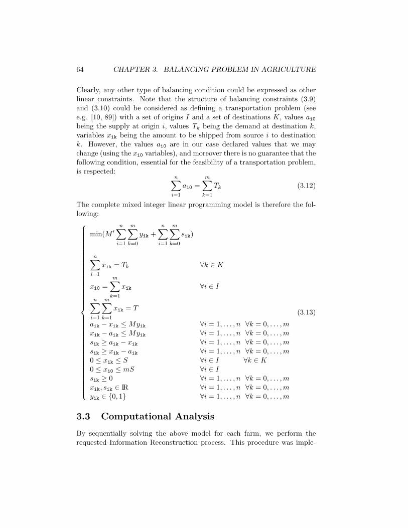
64 CHAPTER 3. BALANCING PROBLEM IN AGRICULTURE
Clearly, any other type of balancing condition could be expressed as otherlinear constraints. Note that the structure of balancing constraints (3.9)and (3.10) could be considered as defining a transportation problem (seee.g. [10, 89]) with a set of origins I and a set of destinations K, values ai0being the supply at origin i, values Tk being the demand at destination k,variables xik being the amount to be shipped from source i to destinationk. However, the values ai0 are in our case declared values that we maychange (using the xi0 variables), and moreover there is no guarantee that thefollowing condition, essential for the feasibility of a transportation problem,is respected:
n∑i=1
ai0 =
m∑k=1
Tk (3.12)
The complete mixed integer linear programming model is therefore the fol-lowing:
min(M ′n∑i=1
m∑k=0
yik +n∑i=1
m∑k=0
sik)
n∑i=1
xik = Tk ∀k ∈ K
xi0 =m∑k=1
xik ∀i ∈ I
n∑i=1
m∑k=1
xik = T
aik − xik ≤Myik ∀i = 1, . . . , n ∀k = 0, . . . ,mxik − aik ≤Myik ∀i = 1, . . . , n ∀k = 0, . . . ,msik ≥ aik − xik ∀i = 1, . . . , n ∀k = 0, . . . ,msik ≥ xik − aik ∀i = 1, . . . , n ∀k = 0, . . . ,m0 ≤ xik ≤ S ∀i ∈ I ∀k ∈ K0 ≤ xi0 ≤ mS ∀i ∈ Isik ≥ 0 ∀i = 1, . . . , n ∀k = 0, . . . ,mxik, sik ∈ IR ∀i = 1, . . . , n ∀k = 0, . . . ,myik ∈ {0, 1} ∀i = 1, . . . , n ∀k = 0, . . . ,m
(3.13)
3.3 Computational Analysis
By sequentially solving the above model for each farm, we perform therequested Information Reconstruction process. This procedure was imple-
3.3. COMPUTATIONAL ANALYSIS 65
mented in C++, using ILOG Concert Technology [66] in order to expressthe described optimization models. The models themselves are solved bymeans of the state-of-the-art branch-and-cut (see e.g. [10, 76]) procedureimplemented by the solver ILOG Cplex [65], running on a 16 cores serverhaving 128Gb of RAM and Linux Operating System. An analysis of thebehavior of open source solvers was published in [11]. The resulting soft-ware system has been applied for the treatment of data from the ItalianCensus of Agriculture 2010 (“Censimento Generale dell’Agricoltura 2010”),with specific respect to the cases of:
1. Vineyards suitable for “controlled origin” wine, considered inTable 3.1;
2. Vineyards not suitable for “controlled origin” wine, considered inTable 3.2;
3. Generic cultivations, considered in Table 3.3;
4. Livestock, considered in Table 3.4.
Note that, in the last two cases, microdata are not subdivided by year ofplanting but by geographical area. In the above four cases, we report resultsfor each Italian region and for all Italy (1st column); the total number offarms not respecting the balancing conditions (2nd column); the total numberof records involved in those unsatisfied balancing conditions (3rd column);the total number of changes operated by the reconstruction process (4th
column).
Moreover, we analyze in greater detail those changes: we report the percent-ages of area (or heads) modified by the procedure, computed with respectto the total area involved in that case (or to the total number of animals).Such modifications can be done by adding (5th column) and/or by subtract-ing (6th column), and note that those quantities are not bounded to beequal, since errors are not so. Finally, we report the total processing timein seconds (7th column).
The practical behavior of the proposed procedure should now be evalu-ated both from the computational and from the data quality points of view.As observable, the procedure is very fast: each single model is solved tooptimality in extremely short times (generally about 0.02 sec.) so that theprocessing of all the Italian farms requires, for the 4 cases together, onlyabout 50 minutes.
The quality of the obtained data has been evaluated by considering: (i)the ability to restore balancing; and (ii) the variation produced in the data

66 CHAPTER 3. BALANCING PROBLEM IN AGRICULTURE
Added SubtractedRegion Farms Records Changes Area Area Time
Piemonte 696 2055 1866 0.15% -1.70% 23.5Valle d’Aosta 22 55 46 0.00% -0.00% 0.6Lombardia 468 1488 1423 0.16% -0.75% 17.0Veneto 3817 6916 5602 4.23% -0.96% 79.2Friuli-Venezia Giulia 286 1528 945 0.13% -0.38% 17.5Liguria 124 257 493 0.01% -0.04% 2.9Emilia-Romagna 336 940 640 0.07% -0.74% 10.8Toscana 3392 6099 4332 3.20% -1.01% 69.8Umbria 73 248 173 0.05% -0.13% 2.8Marche 1359 2243 1541 0.79% -0.21% 25.7Lazio 432 925 1455 0.13% -0.55% 10.6Abruzzo 197 324 300 0.04% -0.36% 3.7Molise 407 479 428 0.12% -0.01% 5.5Campania 420 953 1212 0.13% -0.41% 10.9Puglia 6954 7895 8016 3.04% -0.72% 90.4Basilicata 61 78 104 0.02% -0.06% 0.9Calabria 168 223 369 0.04% -0.12% 2.6Sicilia 620 973 1764 0.43% -0.94% 11.1Sardegna 221 394 668 0.05% -0.45% 4.5Bolzano 125 446 241 0.01% -0.35% 5.1Trento 268 899 482 0.04% -0.34% 10.3Italy total 20346 35418 32100 12.85% -10.21% 405.5
Table 3.1: Vineyards suitable for controlled origin wine.
by the reconstruction process.
As for the first aspect, data obtained by the procedure were able tosatisfy the balancing conditions in the totality of the cases (100%). As forthe second aspect, a positive feature for a general information reconstructionprocedure is satisfying requirements while not changing the data exceedingly.In the analyzed cases, in addition to the theoretical guarantee that thenumber of changes is minimal, we observe that the amount of the variationsis always a small percentage. This means that the procedure was able toreconstruct information without distorting the data.
The accuracy of the reconstructed information has been further evalu-ated by setting up a specific experiment. A large dataset of 274,687 recordsrepresenting all vineyards obtained from about 126,000 farms, all exact,were perturbed by introducing random errors with uniform distribution at3 different intensities, so that respectively about 1%, 5% and 10% of themicrodata values have been changed. This was performed 20 times, in or-der to obtain statistically significant results, so 60 different large erroneousdatasets were obtained. After this, the reconstruction procedure was appliedon all of them, and the 60 obtained (corrected) datasets were compared to
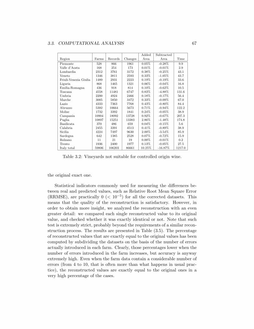
3.3. COMPUTATIONAL ANALYSIS 67
Added SubtractedRegion Farms Records Changes Area Area Time
Piemonte 528 866 1961 0.05% -0.28% 9.9Valle d’Aosta 168 254 173 0.01% -0.01% 2.9Lombardia 2312 3761 3172 0.38% -0.25% 43.1Veneto 1346 3811 2593 0.33% -1.05% 43.7Friuli-Venezia Giulia 1489 2931 2223 0.19% -0.19% 33.6Liguria 868 1465 1321 0.06% -0.04% 16.8Emilia-Romagna 436 918 814 0.10% -0.62% 10.5Toscana 4558 11481 6747 0.83% -4.88% 131.6Umbria 2200 4924 2466 0.18% -0.17% 56.4Marche 3005 5850 3472 0.33% -0.09% 67.0Lazio 4333 7363 7768 0.43% -0.80% 84.4Abruzzo 5392 10664 5673 0.71% -0.94% 122.2Molise 1732 3392 1841 0.24% -0.05% 38.9Campania 10904 18092 13728 0.92% -0.67% 207.3Puglia 10897 15251 13383 2.86% -1.48% 174.8Basilicata 370 486 659 0.04% -0.15% 5.6Calabria 2455 3391 4513 0.41% -0.89% 38.9Sicilia 4224 7497 9630 2.00% -3.54% 85.9Sardegna 642 1385 2528 0.07% -0.72% 15.9Bolzano 11 21 19 0.00% -0.01% 0.2Trento 1936 2400 1977 0.13% -0.05% 27.5Italy total 59806 106203 86661 10.25% -16.87% 1217.0
Table 3.2: Vineyards not suitable for controlled origin wine.
the original exact one.
Statistical indicators commonly used for measuring the differences be-tween real and predicted values, such as Relative Root Mean Square Error(RRMSE), are practically 0 (< 10−5) for all the corrected datasets. Thismeans that the quality of the reconstruction is satisfactory. However, inorder to obtain more insight, we analyzed the reconstruction with an evengreater detail: we compared each single reconstructed value to its originalvalue, and checked whether it was exactly identical or not. Note that suchtest is extremely strict, probably beyond the requirements of a similar recon-struction process. The results are presented in Table (3.5). The percentageof reconstructed values that are exactly equal to the original values has beencomputed by subdividing the datasets on the basis of the number of errorsactually introduced in each farm. Clearly, those percentages lower when thenumber of errors introduced in the farm increases, but accuracy is anywayextremely high. Even when the farm data contain a considerable number oferrors (from 4 to 10, that is often more than what happens in usual prac-tice), the reconstructed values are exactly equal to the original ones in avery high percentage of the cases.

68 CHAPTER 3. BALANCING PROBLEM IN AGRICULTURE
Added SubtractedRegion Farms Records Changes Area Area Time
Piemonte 624 1682 1191 0.037% -0.016% 19.2Valle d’Aosta 84 221 157 0.000% 0.000% 2.5Lombardia 1436 3784 2162 0.030% -0.069% 43.3Veneto 5715 13604 11033 0.383% -0.670% 155.8Friuli-Venezia Giulia 734 1955 1123 0.010% -0.002% 22.4Liguria 264 645 458 0.001% 0.000% 7.3Emilia-Romagna 252 742 976 0.168% -0.042% 8.5Toscana 3006 6571 6274 0.486% -0.319% 75.2Umbria 513 1160 931 0.007% -0.003% 13.2Marche 2210 5347 4615 0.229% -0.088% 61.2Lazio 912 2023 1553 0.009% -0.002% 23.1Abruzzo 1960 4540 2650 0.038% -0.103% 52.0Molise 2006 4649 3817 0.047% -0.035% 53.2Campania 2854 6538 4403 0.015% -0.003% 74.9Puglia 18205 41924 34881 0.561% -0.527% 480.3Basilicata 433 996 710 0.011% -0.005% 11.4Calabria 506 1166 851 0.007% -0.008% 13.3Sicilia 1117 2546 1772 0.035% -0.002% 29.1Sardegna 223 512 407 0.006% -0.004% 5.8Bolzano 23 96 83 0.012% -0.037% 1.1Trento 889 2280 1344 0.005% -0.003% 26.1Italy total 43966 102981 81391 2.098% -1.938% 1180.0
Table 3.3: Other cultivations.
Added SubtractedRegion Farms Records Changes Area Area Time
Piemonte 704 947 719 0.317% -0.107% 9.7Valle d’Aosta 38 51 38 0.000% 0.000% 0.5Lombardia 528 784 574 0.390% -0.130% 8.0Veneto 3797 4449 4489 7.348% -2.763% 45.4Friuli-Venezia Giulia 164 210 169 0.017% -0.285% 2.1Liguria 71 92 71 0.000% 0.000% 0.9Emilia-Romagna 333 593 500 5.585% -8.403% 6.1Toscana 1554 1878 1973 0.265% -0.037% 19.2Umbria 124 160 124 0.000% -0.554% 1.6Marche 1171 1488 1592 0.823% -0.428% 15.2Lazio 302 380 305 0.000% 0.000% 3.9Abruzzo 215 286 217 1.634% 0.000% 2.9Molise 1003 1303 1281 0.437% -0.477% 13.3Campania 387 471 394 0.001% 0.000% 4.8Puglia 3734 4144 4556 0.595% -0.570% 42.3Basilicata 123 173 126 0.001% 0.000% 1.8Calabria 266 320 270 0.000% 0.000% 3.3Sicilia 338 441 340 0.000% 0.000% 4.5Sardegna 276 489 281 0.004% 0.000% 5.0Bolzano 127 181 127 0.000% 0.000% 1.8Trento 97 111 97 0.000% 0.000% 1.1Italy total 15352 18951 18243 17.418% -13.754% 193.5
Table 3.4: Livestock.
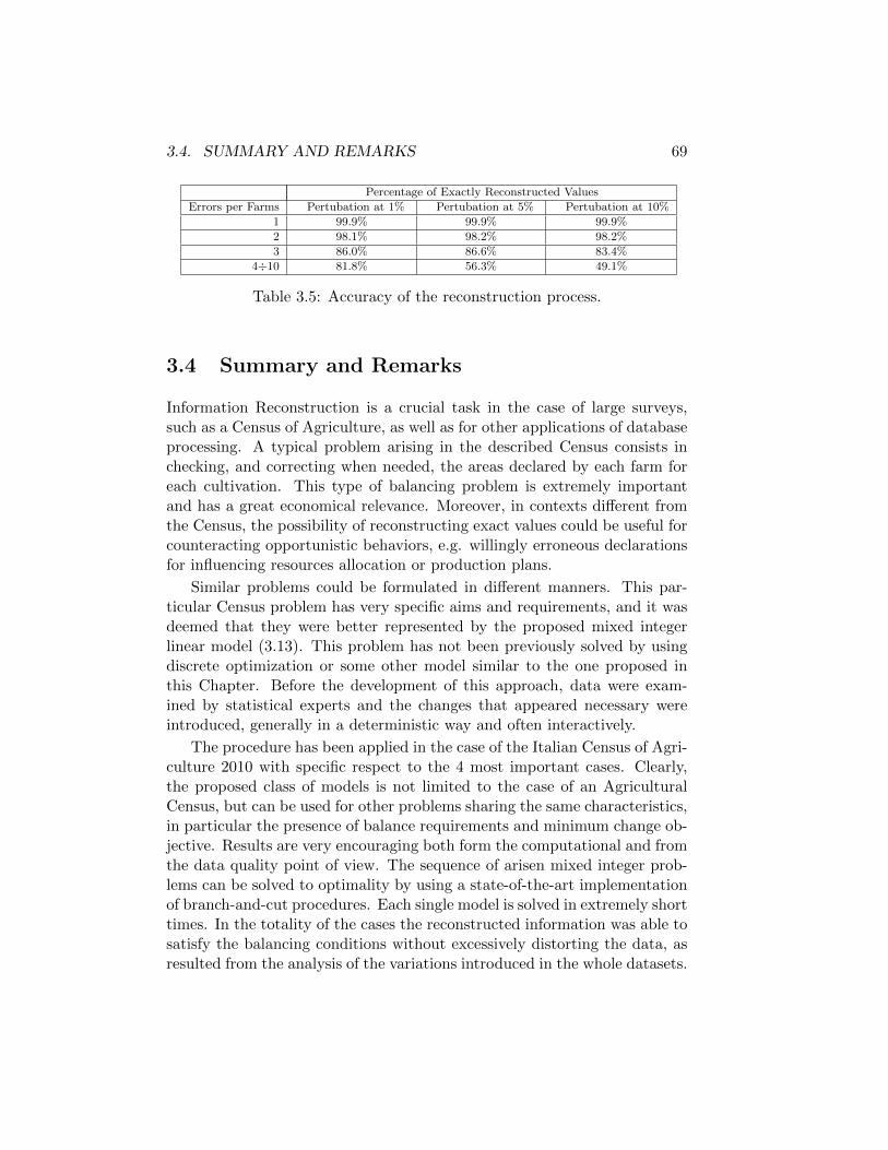
3.4. SUMMARY AND REMARKS 69
Percentage of Exactly Reconstructed Values
Errors per Farms Pertubation at 1% Pertubation at 5% Pertubation at 10%
1 99.9% 99.9% 99.9%
2 98.1% 98.2% 98.2%
3 86.0% 86.6% 83.4%
4÷10 81.8% 56.3% 49.1%
Table 3.5: Accuracy of the reconstruction process.
3.4 Summary and Remarks
Information Reconstruction is a crucial task in the case of large surveys,such as a Census of Agriculture, as well as for other applications of databaseprocessing. A typical problem arising in the described Census consists inchecking, and correcting when needed, the areas declared by each farm foreach cultivation. This type of balancing problem is extremely importantand has a great economical relevance. Moreover, in contexts different fromthe Census, the possibility of reconstructing exact values could be useful forcounteracting opportunistic behaviors, e.g. willingly erroneous declarationsfor influencing resources allocation or production plans.
Similar problems could be formulated in different manners. This par-ticular Census problem has very specific aims and requirements, and it wasdeemed that they were better represented by the proposed mixed integerlinear model (3.13). This problem has not been previously solved by usingdiscrete optimization or some other model similar to the one proposed inthis Chapter. Before the development of this approach, data were exam-ined by statistical experts and the changes that appeared necessary wereintroduced, generally in a deterministic way and often interactively.
The procedure has been applied in the case of the Italian Census of Agri-culture 2010 with specific respect to the 4 most important cases. Clearly,the proposed class of models is not limited to the case of an AgriculturalCensus, but can be used for other problems sharing the same characteristics,in particular the presence of balance requirements and minimum change ob-jective. Results are very encouraging both form the computational and fromthe data quality point of view. The sequence of arisen mixed integer prob-lems can be solved to optimality by using a state-of-the-art implementationof branch-and-cut procedures. Each single model is solved in extremely shorttimes. In the totality of the cases the reconstructed information was able tosatisfy the balancing conditions without excessively distorting the data, asresulted from the analysis of the variations introduced in the whole datasets.

70 CHAPTER 3. BALANCING PROBLEM IN AGRICULTURE
Moreover, a specific experiment proves that the reconstructed informationwas exactly equal to the original uncorrupted one in an exceedingly highpercentage of the cases.

Chapter 4
Reconstruction ofCultivation Data inAgriculture
4.1 Reconstruction of Cultivation Data
Data collected in a Census of Agriculture, as in any other large-scale survey,may contain errors or missing values, and their automatic detection and cor-rection are crucial tasks. This kind of activity is generally called InformationReconstruction, or also Data Cleaning, within the field of Data Mining [61],or Data Editing and Imputation within the field of Statistics [41, 94].
Several approaches to these problems have been developed, dating backto the work of Fellegi-Holt [47]. An approach to verify the accuracy of theseinformations and to restore data consistency is based on the use of rules(edits), that each data record must respect in order to be declared exact[7, 26]. Rules can be converted into linear inequalities, and the problem offinding within a record the most probably erroneous fields or the most suit-able values correcting those fields can be modeled as nontrivial optimizationproblems. This approach allows to overcome the computational limits ofthe Fellegi Holt methodology and it has been implemented within the dataEditing and Imputation software system DIESIS [26, 27].
Agricultural Census data typically are numerical values, such as farmcodes, cultivation codes, size of cultivation areas, etc. Similar data are gen-erally organized into very large numerical records. In the described Census,each farm specifies the cultivation area used for each cultivation. A clas-sical problem is verifying the accuracy of this information. In the event
71
72 CHAPTER 4. CULTIVATION DATA RECONSTRUCTION
that farm declarations are considered unreliable, it’s necessary to assign thecorrect cultivations to the area for which it’s not known. Errors should bedetected and corrected, by mathematically “guessing” the correct values,since it is clearly impossible to contact again the farm or inspect somehowthe cultivations.
Farms can extend on one or more districts, and the area owned by eachfarm in each district is known. Therefore, the compatibility of each culti-vation with each district can also be evaluated (some cultivation can growonly on specific types of soils, or need specific climatic conditions, latitude,altitude, etc.). In the specific case of vineyards, considered in this Chapter,there may be cultivation areas with missing or erroneous vineyard codes.For these areas, it is required to assign a code, according to a set of consis-tency constraints, taking also into account the compatibility between eachdistrict and the type of vineyard. Theoretically, the elements for solving theabove problem are available, but the problem is doing this on large datasetsboth efficiently and in an unbiased manner.
This Chapter presents an innovative automatic procedure for solving thisproblem based on a discrete mathematical optimization model. In partic-ular, Section 4.2 describes problem details and the proposed mixed integerlinear programming model [10, 76], explaining its features. Section 4.3 re-ports computational results in the case of the Italian Census of Agriculture2010, with specific respect to the case of vineyards. This is probably themost important case for the considered problem, since dozens of vine vari-eties exist, and they determine the type and the quality of wines produced.Relevant economic aspects are therefore involved, and vine cultivation anduse are also regulated by legislation. Clearly, the proposed model is notlimited to the case of a Census of Agriculture, but can be used for any otherproblem sharing the same characteristics. This work has been published in[14].
4.2 A Discrete Mathematical Model
Data obtained from each farm during the described Census contain infor-mation about the area used by that farm for each cultivation. Those datamay sometimes be erroneous or missing, due to a variety of reasons. Insuch cases, errors should be automatically detected and corrected, i.e. theinformation that was corrupted and lost should be “reconstructed” in orderto be as similar as possible to the (unknown) exact value.
4.2. A DISCRETE MATHEMATICAL MODEL 73
Farms are located over the state territory. This territory is subdividedinto many districts. Each farm can extend on one or more district. Denoteby
I = {1,. . . , n} the set of all possible cultivations;
J = {1,. . . , m} the set of all possible districts.
Focusing on a single farm, and denoting by f its total area, all the cultiva-tions declared by that farm are checked. Some of them verify a set of rulesand conditions prepared for this aim and are therefore considered reliable,while some other do not. This may happen either because some of the dec-larations appear erroneous, or because there is a discordance between thetotal area declared and the sum of the areas declared for each cultivation.Denote by a the total farm area reliably assigned, i.e. the area for whichthe farm declaration are considered reliable. On the contrary, by groupingall the unreliable declarations, a nonempty area often remains for which thecultivation is not known. That area will be called unassigned area and de-noted by u. Clearly, f = a + u. The central problem of our InformationReconstruction process consist now in assigning the cultivations to the men-tioned unassigned area. In this Section a discrete mathematical model forthis problem is proposed. For each farm, denote by
si (real value ≥ 0) the total area that the farm uses for cultivation i,with i ∈ I. Note that this area may span on one or more districts, andthe farm does not declare, nor generally even consider, such subdivi-sion. These values are only the ones, among all the cultivation datadeclared by farms, that can be considered reliable, so
∑i(si) = a.
dj (real value ≥ 0) the total area owned by the farm in district j, withj ∈ J . These values are not surveyed during the considered Censusbut are already available and are reliable.
pij (real value ∈ [0, 1]) the likelihood of having cultivation i in districtj, with i ∈ I and j ∈ J . Values near to 1 means high likelihood,near to 0 means very low likelihood. This values are estimated on thebasis of agricultural registrations and studies, not surveyed during theconsidered Census.
Moreover, there are areas where specific cultivations may be used to producefoods having “controlled origin” (in Italian DOC). In particular, for theunassigned area u, it is possible to partition it into a portion that is suitable

74 CHAPTER 4. CULTIVATION DATA RECONSTRUCTION
for “controlled origin” and a portion that is not suitable for that. Denoteby
C (reale value ≥ 0) the total unassigned area owned by the farm incultivations suitable for “controlled origin”;
N (real value ≥ 0) the total unassigned area owned by the farm incultivations not suitable for“controlled origin”, so that C +N = u.
Those areas C and N should be assigned in order to maximize the likelihoodof the assignment. Note that it is not known which district the unassignedarea u is located into. On the other hand, the likelihood values depend onthe districts. As a consequence, we need to locate the unassigned area uon the districts. This is apparently hard to obtain. A way of doing so islocating on the districts each of the reliable cultivation areas si, and thenobtaining the location of u as the portion of farm area f not covered by a.In order to model the described problem, we need to introduce the followingsets of decision variables:
xij (real value ≥ 0) the area of cultivation i that, according to ourreconstruction, is localized in district j, with i ∈ I and j ∈ J ;
vij (real value ≥ 0) the portion of C that, according to our reconstruc-tion, is used for cultivation i and localized in district j, with i ∈ I andj ∈ J ;
wij (real value ≥ 0) the portion of N that, according to our recon-struction, is used for cultivation i and localized in district j, with i ∈ Iand j ∈ J .
Moreover, each of the farm unassigned areas C and N generally containsonly a specific cultivation, and not a mixture of different cultivations. Wetherefore want to assign all C to one single type of cultivation, and not tofragment it among all the cultivations compatible with that area. A similarrequirement holds for N . This requires the use of additional binary decisionvariables
yi =
{1 if C is assigned in our reconstruction to cultivation i ,with i ∈ I0 otherwise
zi =
{1 if N is assigned in our reconstruction to cultivation i ,with i ∈ I0 otherwise

4.2. A DISCRETE MATHEMATICAL MODEL 75
Now it’s possible to formulate a mixed integer linear programming modelfor each farm. Cultivation assignment to areas should be done in order tomaximize the likelihood. Our objective function is therefore
max∑∀i,j
pijxij +∑∀i,j
pijvij +∑∀i,j
pijwij (4.1)
This assignment should obviously verify a set of constraints. First of all, thesum of the areas assigned to the different cultivations in each district j mustbe equal to the area owned by the farm in district j:∑
∀ixij +
∑∀i
vij +∑∀i
wij = dj ∀j = 1, . . . ,m (4.2)
The sum of the areas used by the farm for cultivation i over all the districtsmust be equal to the total area used by the farm for cultivation i:∑
∀jxij = si ∀i = 1, . . . , n (4.3)
The sum of the portions of C assigned to all cultivations in all districts mustbe equal to C. A similar condition must hold for N .∑
∀i,jvij = C
∑∀i,j
wij = N (4.4)
In order to connect the y variables to v, we need to impose that it is notpossible assigning a portion of C to cultivation i (regardless to the district)when the corresponding variable yi is 0. A similar condition must hold forto connect the z variables to w. Note that M is a constant value greaterthan all possible left-hand-side values.
vij ≤Myi ∀i = 1, . . . , n ∀j = 1, . . . ,m (4.5)
wij ≤Mzi ∀i = 1, . . . , n ∀j = 1, . . . ,m (4.6)
The whole C must be assigned to only one cultivation. A similar conditionmust hold for N . ∑
∀iyi = 1
∑∀i
zi = 1 (4.7)
76 CHAPTER 4. CULTIVATION DATA RECONSTRUCTION
The above constraints have the effect of letting only one y (only one z) be1, and so the previous constraints can only assigning C (respectively N) toa unique cultivation.
Finally, an assignment for C or for N cannot be accepted when the likeli-hood of that assignment, although being the greatest possible for the currentproblem, is too low. In such a case, indeed, that assignment cannot be con-sidered reliable. For this reason we introduce, in the following constraints,two thresholds, denoted by SC and SN , respectively for the assignmentsmade on C and N .
∑∀j
vij −∑∀j
pijvij − SC ≤M(1− yi) ∀i = 1, . . . , n (4.8)
∑∀j
wij −∑∀j
pijwij − SN ≤M(1− zi) ∀i = 1, . . . , n (4.9)
In the constraints (4.8), the assignment of C can be possible if the likelihoodof assigning C to cultivation i is good (= near to 1) for the different districtswhere C have been located, that means yi can assume value 1. On the otherhand, when that likelihood is not good (= near to 0), that assignment isnot allowed, that means yi must be forced to value 0. Note that, if noassignment has a sufficient likelihood, those constraints cannot be satisfiedand the model correctly becomes infeasible.
The above is obtained because, for assignments having good likelihood, thevalue of
∑∀j pijvij is only a bit smaller than the value of
∑∀j vij, and by
subtracting SC the left-hand-side of the inequality (4.8) becomes smallerthan or equal to 0, leaving yi free.
When on the contrary the likelihood is not good, the value of∑∀j pijvij
is much smaller than the value of∑∀j vij, and even subtracting SC (whose
reasonable value is therefore just a fraction of∑∀j vij, for instance one half)
the left-hand-side of the inequality (4.8) becomes positive. As a consequence,M(1− yi) must have a strictly positive value, and so yi must have value 0.
In the constraints (4.9) the logic of the assignment of N is the same as thatpreviously described for C in the the constraints (4.9).
On the whole, the complete mixed integer linear programming model forassigning the unassigned area of a single farm is the following:

4.3. COMPUTATIONAL RESULTS 77
max∑∀i,j
pijxij +∑∀i,j
pijvij +∑∀i,j
pijwij
∑∀i
xij +∑∀i
vij +∑∀i
wij = dj ∀j = 1, . . . ,m∑∀j
xij = si ∀i = 1, . . . , n∑∀i,j
vij = C∑∀i,j
wij = N
vij ≤Myi ∀i = 1, . . . , n ∀j = 1, . . . ,mwij ≤Mzi ∀i = 1, . . . , n ∀j = 1, . . . ,m∑∀i
yi = 1∑∀i
zi = 1∑∀j
vij −∑∀j
pijvij − SC ≤M(1− yi) ∀i = 1, . . . , n∑∀j
wij −∑∀j
pijwij − SN ≤M(1− zi) ∀i = 1, . . . , n
xij ≥ 0 ∀i = 1, . . . , n ∀j = 1, . . . ,mvij ≥ 0 ∀i = 1, . . . , n ∀j = 1, . . . ,mwij ≥ 0 ∀i = 1, . . . , n ∀j = 1, . . . ,mxij ∈ IR ∀i = 1, . . . , n ∀j = 1, . . . ,mvij ∈ IR ∀i = 1, . . . , n ∀j = 1, . . . ,mwij ∈ IR ∀i = 1, . . . , n ∀j = 1, . . . ,myi ∈ {0, 1} ∀i = 1, . . . , nzi ∈ {0, 1} ∀i = 1, . . . , n
(4.10)
4.3 Computational Results
The requested Information Reconstruction process has been performed bysolving the above model for each farm sequentially. This procedure wasimplemented in C++, using ILOG Concert Technology [66] in order to ex-press the described optimization models. The models themselves are solvedby means of the state-of-the-art branch-and-cut [10, 76] procedure imple-mented by the solver ILOG Cplex [65], running on a 16 cores server having128Gb of RAM and Linux Operating System. The resulting software systemhas been applied for the treatment of data from the Italian Census of Agri-culture 2010, with specific respect to the case of vineyards. This is probably

78 CHAPTER 4. CULTIVATION DATA RECONSTRUCTION
the most important case for the considered problem, since dozens of vinevarieties exist, and they determine the type and the quality of wines pro-duced. The case has therefore great economic relevance and, due to its largedimension, is also computationally demanding. Moreover, the total areathat a region uses for each vine type determines the European Communityfunding obtained for that region. Note that, to the best of our knowledge,no previous attempt to treat this problem with a discrete optimization ap-proach was practically successful. Clearly, the proposed model is not limitedto the case of vineyards, but can be used for any other problem sharing thesame characteristics.
The practical behavior of the proposed procedure has been evaluatedboth from the computational and from the data quality points of view, asfollows. One large dataset including all farms producing vine from all Italianregions has been assembled. This dataset included 388,487 farms, and thetotal number of vineyard areas declared was 804,930, corresponding to atotal area of 625,700 ha (hectares, 1 hectare being 10,000m2). Each vineyarddeclaration constitutes a record, so the dataset is considerably large. Afterthis, the cultivation declarations where checked by means of rules, and anunassigned area resulted for 18,263 farms. The total unassigned area was34,783 ha, with 30,226 ha suitable for “controlled origin” and 4,557 ha notsuitable for “controlled origin”. As remarked in Section 4.1, thresholdswere assigned in order to reject low likelihood cultivation assignments, inparticular SC = 1/2
∑∀j vij and SN = 1/2
∑∀j wij. In order to evaluate
the computational behavior, Table 4.1 reports regional detail, that are: thetotal unassigned area for each region, and the corresponding computationaltimes for processing the whole region. As observable, the procedure is veryfast, and the processing of all the Italian farms having an unassigned arearequires only about 17 minutes.
The quality of the reconstructed information has been evaluated by con-sidering: (i) the ability to assign the unassigned area; and (ii) the variationproduced in the data by the reconstruction process. As for the first aspect,the procedure was able to assign the unassigned area with likelihood val-ues high enough to satisfy the thresholds SC and SN in the totality of thecases (100%). As for the second aspect, Table 4.2 reports an analysis of thepercentages of the two big groups of vine cultivations (red and white) onthe initial data, i.e. before applying the described reconstruction process,and on the final data, i.e. after the reconstruction process, followed by thecomputation of the variation introduced by this process. Note that, in thegeneral case of the correction of a survey, a small variation of the frequencydistributions of the data means that the reconstruction procedure was able
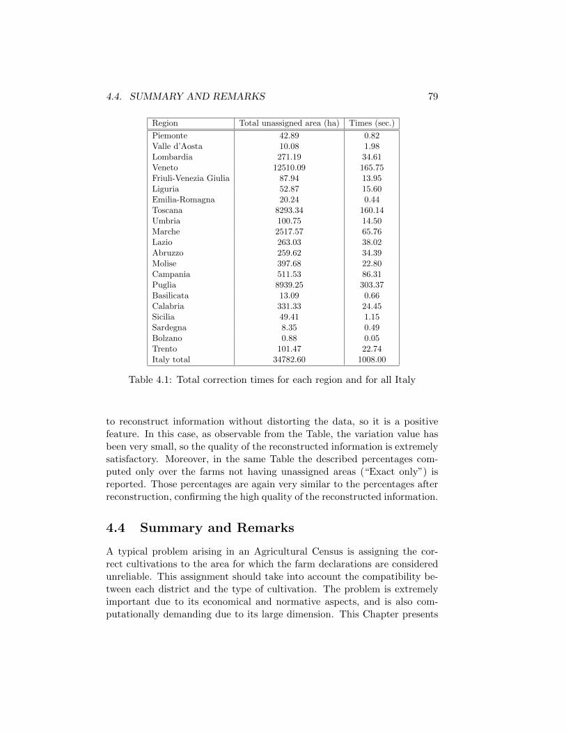
4.4. SUMMARY AND REMARKS 79
Region Total unassigned area (ha) Times (sec.)
Piemonte 42.89 0.82Valle d’Aosta 10.08 1.98Lombardia 271.19 34.61Veneto 12510.09 165.75Friuli-Venezia Giulia 87.94 13.95Liguria 52.87 15.60Emilia-Romagna 20.24 0.44Toscana 8293.34 160.14Umbria 100.75 14.50Marche 2517.57 65.76Lazio 263.03 38.02Abruzzo 259.62 34.39Molise 397.68 22.80Campania 511.53 86.31Puglia 8939.25 303.37Basilicata 13.09 0.66Calabria 331.33 24.45Sicilia 49.41 1.15Sardegna 8.35 0.49Bolzano 0.88 0.05Trento 101.47 22.74Italy total 34782.60 1008.00
Table 4.1: Total correction times for each region and for all Italy
to reconstruct information without distorting the data, so it is a positivefeature. In this case, as observable from the Table, the variation value hasbeen very small, so the quality of the reconstructed information is extremelysatisfactory. Moreover, in the same Table the described percentages com-puted only over the farms not having unassigned areas (“Exact only”) isreported. Those percentages are again very similar to the percentages afterreconstruction, confirming the high quality of the reconstructed information.
4.4 Summary and Remarks
A typical problem arising in an Agricultural Census is assigning the cor-rect cultivations to the area for which the farm declarations are consideredunreliable. This assignment should take into account the compatibility be-tween each district and the type of cultivation. The problem is extremelyimportant due to its economical and normative aspects, and is also com-putationally demanding due to its large dimension. This Chapter presents

80 CHAPTER 4. CULTIVATION DATA RECONSTRUCTION
Before Reconstruction After Reconstruction Variation Exact only
White 43.55% 42.84% -0.71% 43.95%Red 56.45% 57.16% +0.71% 56.05%
Table 4.2: Analysis of frequency distributions before and after the recon-struction process
an automatic approach to this information reconstruction problem based onthe formulation of mixed integer linear programming models. The proposedprocedure has been applied in the specific case of vineyards of the ItalianCensus of Agriculture 2010. In this important case there may be areas withmissing or erroneous vineyard codes. For these areas, it is required to as-sign a code, according to a set of consistency constraints. Results are veryencouraging both form the computational and from the data quality pointof view. The sequence of arisen mixed integer programming problems canbe solved to optimality by using state-of-the-art implementation of branch-and-cut procedures. Each single model is solved to optimality in extremelyshort times (generally about 0.1 sec.). In the totality of the cases the re-constructed information was able to satisfy the thresholds introduced toreject low likelihood cultivation assignments. Moreover, the reconstructionprocess did not distort data, as resulted from the analysis of the variationsintroduced in the frequency distributions of the whole dataset. The method-ology described in this Chapter can again be used to solve other problemsof different origin but having the same mathematical structure.
Chapter 5
A Formal Procedure forFinding Contradictions intoa Set of Rules
5.1 The Problem of Contradictions Localization
In several fields of knowledge, many tasks are accomplished by using sets ofexpressions called rules (see e.g. [47]). Rules are typically used do detect,among a possibly large set of elements, the ones verifying some condition.This happens for example in Data Mining, in Database Theory, in Statis-tics, but also in less mathematical fields such as Normative or Regulation.The condition may be of any nature, for instance ”being correct”, ”beingwrong”, ”being convenient”, ”respecting the laws”, ”being compliant with astandard”, etc. The set of rules may have several origins: it could be auto-matically generated, for instance learned by some dataset, or be written byhuman experts, or also be the result of an updating or a merging of othersets of rules. A major issue is the presence of contradictions into the set ofrules itself. This can frequently arise, in particular when the set of rules hasbeen assembled from different sources. Generally, the presence of contra-dictions makes such a set not usable anymore. Each contradiction shouldtherefore be located and removed, either by deleting or by slightly changingsome of the rules. This is however a very difficult problem in general: a con-tradiction can be quite hidden, or involve many rules, or there can be severalcontradictions. Moreover, this difficulty rapidly increases with the size ofthe set of rules [52]. See also [25, 28] for related work on inconsistenciesselection.
81

82 CHAPTER 5. FINDING CONTRADICTIONS IN A SET OF RULES
This Chapter presents an automatic procedure for finding a contradic-tion into a set of rules. The procedure can be iterated until all contradictionsare removed from a set. A main advantage of the proposed approach is thatthis procedure works only at the formal level, so it can be performed with-out the need of going into the semantic meaning of the rules under analysisand can be applied to rules arising from any field. In particular, Section 5.2explains how several kind of rules can be formally represented into linearinequalities. After this, Section 5.3 presents a theoretical condition, basedon a variant of Farkas’ lemma (see e.g. [88]), used to detect a single con-tradiction. All contradictions are detected by iterating this procedure, andthe structure of the set of all contradictions, together with the relationshipsamong themselves, are also studied. Finally, Section 5.4 gives a detailedexplanation of the operations performed by the proposed procedure on arealistic set of rules. This work has been published in [12].
5.2 Encoding Rules into Linear Inequalities
In Database theory, a record schema is a set of fields fi, with i = 1 . . .m,and a record instance is a set of values vi, one for each of the above fields. Inorder to help exposition, we will focus on records representing persons. Note,however, that the proposed procedure is not influenced by the meaning ofprocessed data. The record scheme will be denoted by P , whereas a genericrecord instance corresponding to P will be denoted by p.
P = {f1, . . . , fm} p = {v1, . . . , vm}
Example 5.1. For records representing persons, fields are for instance age
or marital status, and corresponding examples of values are 18 or single.
Each field fi, with i = 1 . . .m, has its domain Di, which is the set of everypossible value for that field. A distinction is usually made between quantita-tive, or numerical, fields, and qualitative, or categorical, fields. The proposedapproach is able to deal with both qualitative and quantitative values.
In several applications, records verifying some condition are selected byusing rules. As known in Section 1.4, each rule can be seen as a mathematicalfunction rk from the Cartesian product of all the domains to the Booleanset {0,1}, as follows.
rk : D1 × · · · ×Dm → {0, 1}p 7→ 0, 1
5.2. ENCODING RULES INTO LINEAR INEQUALITIES 83
We call logical rules the rules expressed only with logical conditions, math-ematical rules the rules expressed only with mathematical conditions, andlogic-mathematical rules the rules expressed using both types of condition.See [26] for further details on different kind of rules.
Values appearing in the rules are called breakpoints, or cut points, for thedomains. They represent the logical watershed between values of the domain,and will be indicated with bji . Such breakpoints are used to split every
domain Di into ni subsets Sji representing values of the domain which are
equivalent from the rules’ point of view. We congruently have Di =⋃nij=1 S
ji .
Example 5.2. Suppose that, by scanning a given set of rules R, the follow-ing breakpoints are obtained for the field age of a person.
b1age = 0, b2age = 14, b3age = 18, b4age = 26, b5age = 110, b6age = blank
and, by using the breakpoints and the rules to cut Dage, we have the nage = 5subsets. The last subset is the out-of-range one.
Sage∈{0...13} = {0, . . . , 13}, Sage∈{14...17} = {14, . . . , 17},Sage∈{18...25} = {18, . . . , 25}, Sage∈{26...110} = {26, . . . , 110},
Sage = out of range = {. . . ,−1} ∪ {111, . . . } ∪ {blank}
Now, the variables for the announced linear inequalities can be introduced:a set of m real variables zi ∈ [0, U ], one for each domain Di, and a set ofn = n1 + · · ·+ nm binary variables xij ∈ {0, 1}, one for each subset Sij . Werepresent each value vi of p with a real variable zi, by defining a mappingϕ between values of the domain and real numbers between 0 and an uppervalue U . Note that, occasionally, it could be convenient to bound someof the zi variables to be integer, as described in [26], with obvious specificmodifications in the rest of the procedure. However, in this description weconsider the general case of real z variables.
The membership of a value vi to the subset Sij is encoded by using thebinary variables xij .
xij =
{1 when vi ∈ Sij0 when vi 6∈ Sij
Binary and real variables are linked by using a set of linear inequalitiescalled bridge constraints. They impose that, when zi has a value such thatvi belongs to subset Sij , the corresponding xij is 1 and all others binary
84 CHAPTER 5. FINDING CONTRADICTIONS IN A SET OF RULES
variables {xi1, . . . , xij−1, xij+1, . . . , xini} of field fi are 0. By using thesevariables, all the above types of rule can be expressed. For further detailssee [26, 27].
Example 5.3. Consider the following logical rule.
¬(marital status = married) ∨ ¬(age < 14)
By substituting the logical conditions, it becomes the linear inequality:
(1− xmarital status = married) + (1− xage∈{0...13}) ≥ 1
Consider, instead, the following logic-mathematical rule.
¬(marital status = married) ∨ (age− years married ≥ 14)
By substituting the logical and mathematical conditions, we have
(1− xmarital status = married) ∨ (zage − zyears married ≥ 14)
which becomes the following linear inequality
U(1− xmarital status = married) + zage − zyears married ≥ 14
Altogether, from the set of rules R, a set of linear inequalities is obtained.Each record p determines an assignment of values for the introduced vari-ables xij and zi. By denoting with x and z the vectors respectively made ofall the components xij and zi, i = 1 . . .m, j = 1 . . . ni, as follows,
x = (x11, . . . , x1n1 , . . . , xm1, . . . , xmnm)T z = (z1, . . . , zm)T
the set of rules R becomes a system of linear inequalities, expressed in com-pact notation as follows.
B
[xz
]≥ b
0 ≤ zi ≤ U i = 1 . . .mx ∈ {0, 1}nz ∈ IRm
(5.1)
Since x has n = n1 + ... + nm components and z has m components, andletting l be the total number of inequalities, B is in general a l × (n + m)real matrix, and b a real l-vector.

5.3. LOCATING CONTRADICTIONS BYMEANS OF LINEAR PROGRAMMING 85
5.3 Locating Contradictions by Means of LinearProgramming
A contradiction in the set of rules corresponds to an unsatisfiable set ofinequalities within the above described system of linear inequalities. Suchan unsatisfiable set is called Infeasible Subsystem (IS). When an IS is mini-mal, i.e. becomes satisfiable by removing anyone of its inequalities, is calledIrreducible Infeasible Subsystem(IIS) [3, 35, 90]. In the case of systems oflinear inequalities having real variables, the problem has been approachedboth by means of heuristics [34] and exact algorithms [55]. In the case ofsystems of linear inequalities having integer variables (more computation-ally demanding), the problem has been approached by means of additive orsubtractive heuristics [56]. This Chapter presents a procedure for solvingthis problem based on a variant of well known Farkas’ lemma adapted fromthe continuous to the discrete case.
Theorem 5.1. (Farkas’ lemma) Let A be an s × t real matrix and let abe a real s-vector. Then there exists a real t-vector x ≥ 0 with Ax = a ifand only if yTa ≥ 0 for each real s-vector y with yTA ≥ 0.
Geometrically, this means that if an s-vector γ does not belong to the conegenerated by the s-vectors a1, . . . , at (columns of A), there exists a linearhyperplane separating γ from a1, . . . , at. There are several equivalent formsof Farkas’ lemma. The following variant is more suitable to our purposes.Given a matrix A ∈ IRs×t and a vector a ∈ IRs, consider the system:{
Ax ≤ ax ∈ IRt (5.2)
and the new system of linear inequalities obtained from the former one:yTA = 0yTa < 0y ≥ 0y ∈ IRs
(5.3)
We have that exactly one of the two following possibilities holds:
• (5.2) is feasible, i.e. there exists x ∈ IRt verifying all its inequalities.
• (5.3) is feasible, i.e. there exists y ∈ IRs verifying all its inequalities.

86 CHAPTER 5. FINDING CONTRADICTIONS IN A SET OF RULES
An IIS can be selected within (5.2) by solving the following new system [55]:yTA = 0yTa ≤ −1y ≥ 0y ∈ IRs
(5.4)
The support of a vertex denotes the indices of its non-zero components; 0,1 and U respectively denote vectors of zeros, ones and Us of appropriatedimension.
Theorem 5.2. (Gleeson and Ryan) Consider two systems of linear in-equalities respectively in form (5.2) and (5.4). If (5.4) is infeasible, (5.2)is feasible. On the contrary, if (5.4) is feasible, (5.2) is infeasible, and,moreover, each IIS of (5.2) is given by the support of each vertex of thepolyhedron (5.4).
The proof is based on polyhedral arguments using properties of extremerays, see [55]. Therefore, checking the feasibility of (5.2), and, if infeasible,identifying one of its IIS, becomes the problem of finding a vertex of apolyhedron, that can be easily solved (e.g. with the simplex algorithm [10,88]).
However, in the case of (5.1), we have a systems of linear inequalitieswere we are interested in mixed integer solutions. In order to use the resultsgiven for the linear case, let us consider the linear relaxation of such system(5.1).
−B[xz
]≤ −b[
xz
]≤
[1U
]−[xz
]≤ 0[
xz
]∈ IRn+m
(5.5)
The above system (5.5) is now in the form of (5.2). The l inequalities fromthe first group will be called rules inequalities, even if, for some of them,there can be no one-to-one correspondence with rules (see Sect. 5.4). Bydenoting with I the identity matrix, the [l+ 2(n+m)]× (n+m) matrix Aand the [l + 2(n + m)]-vector a are composed as follows. Number of rowsfor each block is reported on the left.

5.3. LOCATING CONTRADICTIONS BY MEANS OF LP 87
A =
−BI−I
ln+mn+m
a =
−b
1U0
lnm
n+m
Therefore, a system which plays the role of (5.4) can now be written.
yT
−BI−I
= 0
yT
−b
1U0
≤ −1
y ≥ 0, y ∈ IR[l+2(n+m)]
(5.6)
So far, the following result on the pair of systems (5.1) and (5.6) holds.The restriction of the support of a vertex to rules inequalities will denotethe indices of its non-zero components among those corresponding to rulesinequalities.
Theorem 5.3. Consider two systems of linear inequalities respectively inform (5.1) and (5.6). In this case, if (5.6) is feasible, (5.1) is infeasible, andthe restriction of the support of each vertex of the polyhedron (5.6) to rulesinequalities contains an IIS of (5.1). On the contrary, if (5.6) is infeasible,(5.5) is feasible, but it cannot be decided whether (5.1) is feasible or not.
Proof: We first prove that the restriction of the support of a vertex of(5.6) to rule inequalities contains an integer IIS of (5.1). Assume (5.6) isfeasible, and let v1 be the vertex found. Therefore, (5.5) is infeasible (fromTheorem 5.1), and an IIS in (5.5), called in this Chapter IIS 1, is givenby the support of v1. Such IIS 1 is in general composed by a set RI 1 ofrules inequalities and a set BC1 (possibly empty) of box constraints (theones imposing 0 ≤ xij ≤ 1, 0 ≤ zi ≤ U). The set of inequalities RI 1 hasno integer solutions, since removing the BC 1 from IIS 1, while imposingthe more strict integer constraints IC 1 (the ones imposing xij ∈ {0, 1}),keeps IIS 1 unsatisfiable. Therefore, an integer IIS is contained into RI1.The integer IIS may also be a subset of the inequalities of RI1, because,though IIS 1 = RI1 ∪ BC1 is minimally infeasible, RI1 ∪ IC1 may be notminimal: we are imposing the more strict integer constraints instead of the
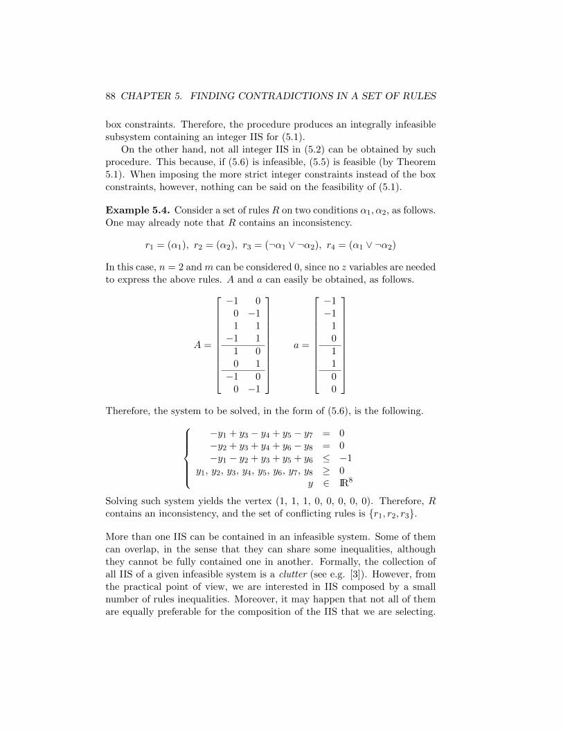
88 CHAPTER 5. FINDING CONTRADICTIONS IN A SET OF RULES
box constraints. Therefore, the procedure produces an integrally infeasiblesubsystem containing an integer IIS for (5.1).
On the other hand, not all integer IIS in (5.2) can be obtained by suchprocedure. This because, if (5.6) is infeasible, (5.5) is feasible (by Theorem5.1). When imposing the more strict integer constraints instead of the boxconstraints, however, nothing can be said on the feasibility of (5.1).
Example 5.4. Consider a set of rules R on two conditions α1, α2, as follows.One may already note that R contains an inconsistency.
r1 = (α1), r2 = (α2), r3 = (¬α1 ∨ ¬α2), r4 = (α1 ∨ ¬α2)
In this case, n = 2 and m can be considered 0, since no z variables are neededto express the above rules. A and a can easily be obtained, as follows.
A =
−1 00 −11 1−1 1
1 00 1
−1 00 −1
a =
−1−1
10
11
00
Therefore, the system to be solved, in the form of (5.6), is the following.
−y1 + y3 − y4 + y5 − y7 = 0−y2 + y3 + y4 + y6 − y8 = 0−y1 − y2 + y3 + y5 + y6 ≤ −1
y1, y2, y3, y4, y5, y6, y7, y8 ≥ 0y ∈ IR8
Solving such system yields the vertex (1, 1, 1, 0, 0, 0, 0, 0). Therefore, Rcontains an inconsistency, and the set of conflicting rules is {r1, r2, r3}.
More than one IIS can be contained in an infeasible system. Some of themcan overlap, in the sense that they can share some inequalities, althoughthey cannot be fully contained one in another. Formally, the collection ofall IIS of a given infeasible system is a clutter (see e.g. [3]). However, fromthe practical point of view, we are interested in IIS composed by a smallnumber of rules inequalities. Moreover, it may happen that not all of themare equally preferable for the composition of the IIS that we are selecting.

5.3. LOCATING CONTRADICTIONS BY MEANS OF LP 89
Hence, a cost ck for taking each of the [l + 2(n + m)] inequalities into ourIIS can be assigned. Such costs ck for the inequalities of (5.5) correspondsto costs for the variables of system (5.6). A cost [l + 2(n + m)]-vectorc is therefore computed, and the solution of the following linear programproduces now an IIS having the desired inequality composition.
min cT y
yT
−BI−I
= 0
yT
−b
1U0
≤ −1
y ≥ 0, y ∈ IR[l+2(n+m)]
(5.7)
The result of Theorem 5.3 is not completely analogous to the linear case. Inorder to obtain more analogy, let us define the following property.
Integral-point property. A class of polyhedra which, if non-empty, con-tain at least one integral point (i.e. a point respecting integrality constraints)has the integral-point (IP) property.
Theorem 5.4. If the polyhedron (5.5), which is the linear relaxation of(5.1), has the integral-point property, the following holds. If (5.6) is infea-sible, (5.1) is feasible. On the contrary, if (5.6) is feasible, (5.1) is infeasibleand each integer IIS is given by the restriction of the support of each vertexof polyhedron (5.6) to rules inequalities.
Proof: If (5.6) is infeasible, (5.5) is feasible by Theorem 5.1. Since we as-sumed that the IP-property holds for (5.5), it contains at least one integralpoint. Since the box constraints hold for (5.5), this integer point must besuch that x ∈ {0, 1}n, hence (5.1) is feasible. On the contrary, if (5.6) isfeasible, the restriction of the support of a vertex in (5.6) to rule inequali-ties, that is a set of inequalities denoted by RI1, has no integer solutions byTheorem 5.3. We now prove by contradiction that RI1 is minimally infea-sible, hence it is an integer IIS. Suppose RI1 not minimal; then there existsa smaller set RI ′1 such that RI ′1 ∪ IC1 has no integer solutions. On theother hand, by Theorem 5.2, RI1 ∪BC1 is minimal, so RI ′1 ∪BC1 must be

90 CHAPTER 5. FINDING CONTRADICTIONS IN A SET OF RULES
feasible, and since it has the IP-property, it has an integer solution, whichis the contradiction. The thesis follows.
So far, when the IP property holds, solving a linear programming prob-lem solves our inconsistency selection problem. There are several cases inwhich the linear relaxation (5.5) defines a polyhedron having the integral-point property (see e.g. [30, 36, 76]). Note that, imposing some syntacticrestrictions, rules could be written in order to obtain one of such cases.
5.4 Applying the Proposed Procedure
Assume that each individual is described by a data record (a set of valuesfor a set of fields). Let the fields be either categorical, e.g. name, profes-sion, tax1 (= if the individual has to pay a tax called tax1), tax2, tax3, ornumerical, e.g. age, length of career, income.
Let the domain of profession be a set of strings (e.g. pr1, pr2, pr3); blankbeing an admissible value, e.g. for non-working people); the domain of tax1,tax2, tax3 be {yes, no}; the domain of age be a suitable subset of the set ofreal non-negative numbers IR+ (or of Z+, with obvious modifications); thedomain of length of career be a suitable subset of IR+ ∪ blank (blank beingan admissible value, e.g. for non-working people); the domain of income bea suitable subset of R+ (being 0 for non-working people).
Assume there is a set of rules for economical regulation (something sim-ilar to laws), as follows. Clearly, the focus is not on numerical values ap-pearing in the rules, that may be unrealistic, but on the structure of the set.Note that, in order to test the consistency of this set, we need to consideralso rules that a human would consider obvious, but not a machine, calledunexpressed rules.
• Logical rules
Some taxes must be paid for some professions
L1 if profession = (pr1 or pr2) then tax1 must be yes
L2 if profession = pr3 then tax2 must be yes
Some taxes must be paid for some income values
L3 if income ≥ 1000 then tax3 must be yes
For poor people taxes cannot exceed 100

5.4. APPLYING THE PROPOSED PROCEDURE 91
L4 if income ≤ 200 then total tax must be ≤ 100
• Mathematical rules
Income must be related to length of career
M1 income ≤ 1000 + 20×length of career
M2 income ≥ 200 + 30×length of career
Taxes must be at least one third of the income
M3 total tax ≥ 0.33×income
Taxes cannot exceed income
M4 total tax ≤income
• Logico-mathematical rules
If income is too high for the career, tax 3 must me paid
LM1 if income −30×length of career ≥ 400 then tax3 must be yes
• Unexpressed rules
Professions are mutually exclusive
U1 Pr1 ⊕Pr2 ⊕Pr3
There are relations implied by the meaning of the words
U2 total tax = tax1+tax2+tax3
Some Fields are naturally limited
U3 age ≥ 0 and ≤ 110
U4 length of career ≥ 0 and ≤ 92
U5 ε ≥ 0 and ≤ 0.001
U6 total tax ≥ 0 and ≤ 2000
U7 income ≥ 0 and ≤ 5000
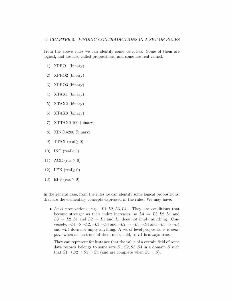
92 CHAPTER 5. FINDING CONTRADICTIONS IN A SET OF RULES
From the above rules we can identify some variables. Some of them arelogical, and are also called propositions, and some are real-valued.
1) XPRO1 (binary)
2) XPRO2 (binary)
3) XPRO3 (binary)
4) XTAX1 (binary)
5) XTAX2 (binary)
6) XTAX3 (binary)
7) XTTAX0-100 (binary)
8) XINC0-200 (binary)
9) TTAX (real≥ 0)
10) INC (real≥ 0)
11) AGE (real≥ 0)
12) LEN (real≥ 0)
13) EPS (real≥ 0)
In the general case, from the rules we can identify some logical propositions,that are the elementary concepts expressed in the rules. We may have:
• Level propositions, e.g. L1, L2, L3, L4. They are conditions thatbecome stronger as their index increases, so L4 ⇒ L3, L2, L1 andL3 ⇒ L2, L1 and L2 ⇒ L1 and L1 does not imply anything. Con-versely, ¬L1⇒ ¬L2,¬L3,¬L4 and ¬L2⇒ ¬L3,¬L4 and ¬L3⇒ ¬L4and ¬L4 does not imply anything. A set of level propositions is com-plete when at least one of them must hold, so L1 is always true.
They can represent for instance that the value of a certain field of somedata records belongs to some sets S1, S2, S3, S4 in a domain S suchthat S1 ⊇ S2 ⊇ S3 ⊇ S4 (and are complete when S1 = S).

5.4. APPLYING THE PROPOSED PROCEDURE 93
• Exclusive propositions, e.g. E1, E2, E3. They are mutually exclusive:at most one of them holds, so E1 ⇒ ¬E2,¬E3 and E2 ⇒ ¬E1,¬E3and E3 ⇒ ¬E1,¬E2. Equivalently, ¬E1 ∨ ¬E2 and ¬E2 ∨ ¬E3 and¬E1 ∨ ¬E3. A set of exclusive propositions is complete when at leastone of them must hold, so E1 ∨ E2 ∨ E3.
They can represent for instance that the value of a certain field of somedata records belongs to some sets S1, S2, S3 such that S1 ∩ S2 = φand S2∩S3 = φ and S1∩S3 = φ (complete when S1∪S2∪S3 = S).
• Standard propositions, e.g. F,G,H, I. They have no predefined re-lations among them, and any relation among them can be expressed,e.g. F ⇒ G and F ∧H ⇒ I.
The rules may contain one or more inconsistencies, as explained in Section5.3. Note that inconsistencies may be either complete, when no record canrespect the rules, or partial, when no record having a specific value vi for aspecific field i (value that should not be forbidden) can respect the rules. Inthis example we have:
• No complete inconsistency: there are records respecting all the rules.
• A partial inconsistency for length of career ≥ 67(M2 says income ≥ 2210 and M3 says total tax ≥ 729.3, while U2 saystotal tax can be at most 720 when all tax1, tax2, tax3 are paid. SinceU7 says 0 ≤ income ≤ 5000, that is a contradiction).
• Another partial inconsistency for length of career ≥ 81(M1 says income ≤ 2620 while M2 says income ≥ 2630, that is acontradiction).
• Another partial inconsistency for income ≥ 2182(M3 says total tax ≥ 720.06, while U2 says total tax can be at most 720when all tax1, tax2, tax3 are paid. Since U7 says 0 ≤ income ≤ 5000,that is a contradiction).
Partial inconsistencies can be tested with the proposed procedure by simplyimposing the value activating them, for instance by adding a constraint. Wenow analyze the above three examples with our procedure. First we convertrules into inequalities, until putting all of them in the form ≤
L1 if profession = (pr1 or pr2) then tax1 must be yes
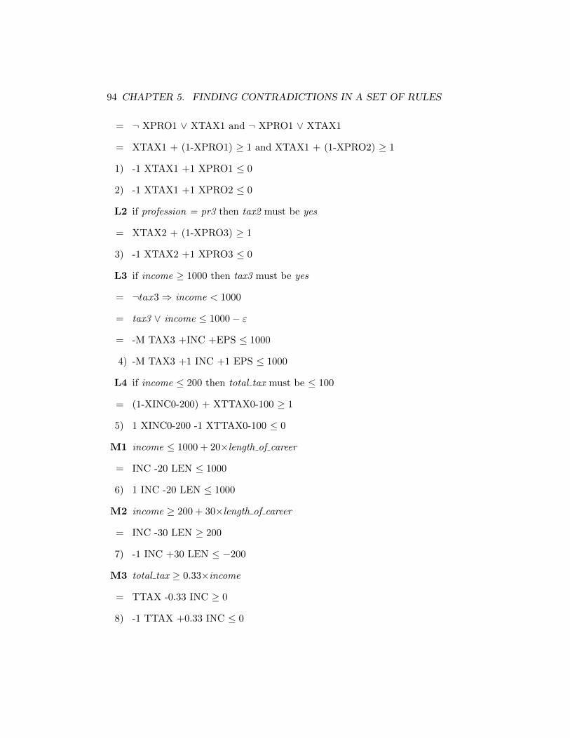
94 CHAPTER 5. FINDING CONTRADICTIONS IN A SET OF RULES
= ¬ XPRO1 ∨ XTAX1 and ¬ XPRO1 ∨ XTAX1
= XTAX1 + (1-XPRO1) ≥ 1 and XTAX1 + (1-XPRO2) ≥ 1
1) -1 XTAX1 +1 XPRO1 ≤ 0
2) -1 XTAX1 +1 XPRO2 ≤ 0
L2 if profession = pr3 then tax2 must be yes
= XTAX2 + (1-XPRO3) ≥ 1
3) -1 XTAX2 +1 XPRO3 ≤ 0
L3 if income ≥ 1000 then tax3 must be yes
= ¬tax3⇒ income < 1000
= tax3 ∨ income ≤ 1000− ε
= -M TAX3 +INC +EPS ≤ 1000
4) -M TAX3 +1 INC +1 EPS ≤ 1000
L4 if income ≤ 200 then total tax must be ≤ 100
= (1-XINC0-200) + XTTAX0-100 ≥ 1
5) 1 XINC0-200 -1 XTTAX0-100 ≤ 0
M1 income ≤ 1000 + 20×length of career
= INC -20 LEN ≤ 1000
6) 1 INC -20 LEN ≤ 1000
M2 income ≥ 200 + 30×length of career
= INC -30 LEN ≥ 200
7) -1 INC +30 LEN ≤ −200
M3 total tax ≥ 0.33×income
= TTAX -0.33 INC ≥ 0
8) -1 TTAX +0.33 INC ≤ 0
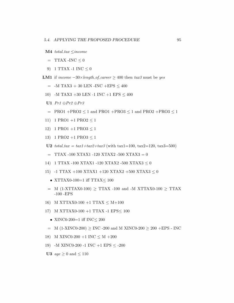
5.4. APPLYING THE PROPOSED PROCEDURE 95
M4 total tax ≤income
= TTAX -INC ≤ 0
9) 1 TTAX -1 INC ≤ 0
LM1 if income −30×length of career ≥ 400 then tax3 must be yes
= -M TAX3 + 30 LEN -INC +EPS ≤ 400
10) -M TAX3 +30 LEN -1 INC +1 EPS ≤ 400
U1 Pr1 ⊕Pr2 ⊕Pr3
= PRO1 +PRO2 ≤ 1 and PRO1 +PRO3 ≤ 1 and PRO2 +PRO3 ≤ 1
11) 1 PRO1 +1 PRO2 ≤ 1
12) 1 PRO1 +1 PRO3 ≤ 1
13) 1 PRO2 +1 PRO3 ≤ 1
U2 total tax = tax1+tax2+tax3 (with tax1=100, tax2=120, tax3=500)
= TTAX -100 XTAX1 -120 XTAX2 -500 XTAX3 = 0
14) 1 TTAX -100 XTAX1 -120 XTAX2 -500 XTAX3 ≤ 0
15) -1 TTAX +100 XTAX1 +120 XTAX2 +500 XTAX3 ≤ 0
• XTTAX0-100=1 iff TTAX≤ 100
= M (1-XTTAX0-100) ≥ TTAX -100 and -M XTTAX0-100 ≥ TTAX-100 -EPS
16) M XTTAX0-100 +1 TTAX ≤ M+100
17) M XTTAX0-100 +1 TTAX -1 EPS≤ 100
• XINC0-200=1 iff INC≤ 200
= M (1-XINC0-200) ≥ INC -200 and M XINC0-200 ≥ 200 +EPS - INC
18) M XINC0-200 +1 INC ≤ M +200
19) -M XINC0-200 -1 INC +1 EPS ≤ -200
U3 age ≥ 0 and ≤ 110

96 CHAPTER 5. FINDING CONTRADICTIONS IN A SET OF RULES
= AGE ≥ 0 and AGE ≤ 110
20) -1 AGE ≤ 0 21) 1 AGE ≤ 110
U4 length of career ≥ 0 and ≤ 92
= LEN ≥ 0 and LEN ≤ 92
22) -1 LEN ≤ 0 23) 1 LEN ≤ 92
U5 ε ≥ 0 and ≤ 0.001
= EPS ≥ 0 and EPS ≤ 0.001
24) -1 EPS ≤ 0 25) 1 EPS ≤ 0.001
U6 total tax ≥ 0 and ≤ 2000
= TTAX ≥ 0 and ≤ 2000
26) -1 TTAX ≤ 0 27) 1 TTAX ≤ 2000
U7 income ≥ 0 and ≤ 5000
= INC ≥ 0 and INC ≤ 5000
28) -1 INC ≤ 0 29) 1 INC ≤ 5000
• XPRO1 binary
30) -1 XPRO1 ≤ 0 31) 1 XPRO1 ≤ 1
• XPRO2 (binary)
32) -1 XPRO2 ≤ 0 33) 1 XPRO2 ≤ 1
• XPRO3 (binary)
34) -1 XPRO3 ≤ 0 35) 1 XPRO3 ≤ 1
• XTAX1 (binary)
36) -1 XTAX1 ≤ 0 37) 1 XTAX1 ≤ 1
• XTAX2 (binary)
38) -1 XTAX2 ≤ 0 39) 1 XTAX2 ≤ 1

5.4. APPLYING THE PROPOSED PROCEDURE 97
• XTAX3 (binary)
40) -1 XTAX3 ≤ 0 41) 1 XTAX3 ≤ 1
• XTTAX0-100 (binary)
42) -1 XTTAX0-100 ≤ 0 43) 1 XTTAX0-100 ≤ 1
• XINC0-200 (binary)
44) -1 XINC0-200 ≤ 0 45) 1 XINC0-200 ≤ 1
Overall, we have the following set of linear inequalities in form ≤
1) -1 XTAX1 +1 XPRO1 ≤ 0
2) -1 XTAX1 +1 XPRO2 ≤ 0
3) -1 XTAX2 +1 XPRO3 ≤ 0
4) -M TAX3 +1 INC +1 EPS ≤ 1000
5) 1 XINC0-200 -1 XTTAX0-100 ≤ 0
6) 1 INC -20 LEN ≤ 1000
7) -1 INC +30 LEN ≤ −200
8) -1 TTAX +0.33 INC ≤ 0
9) 1 TTAX -1 INC ≤ 0
10) -M TAX3 +30 LEN -1 INC +1 EPS ≤ 400
11) 1 PRO1 +1 PRO2 ≤ 1
12) 1 PRO1 +1 PRO3 ≤ 1
13) 1 PRO2 +1 PRO3 ≤ 1
14) 1 TTAX -100 XTAX1 -120 XTAX2 -500 XTAX3 ≤ 0
15) -1 TTAX +100 XTAX1 +120 XTAX2 +500 XTAX3 ≤ 0
16) M XTTAX0-100 +1 TTAX ≤ M+100
17) M XTTAX0-100 +1 TTAX -1 EPS≤ 100
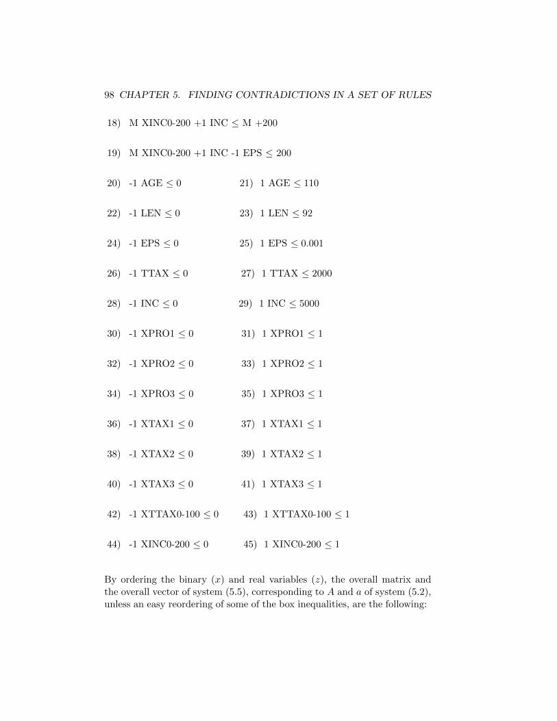
98 CHAPTER 5. FINDING CONTRADICTIONS IN A SET OF RULES
18) M XINC0-200 +1 INC ≤ M +200
19) M XINC0-200 +1 INC -1 EPS ≤ 200
20) -1 AGE ≤ 0 21) 1 AGE ≤ 110
22) -1 LEN ≤ 0 23) 1 LEN ≤ 92
24) -1 EPS ≤ 0 25) 1 EPS ≤ 0.001
26) -1 TTAX ≤ 0 27) 1 TTAX ≤ 2000
28) -1 INC ≤ 0 29) 1 INC ≤ 5000
30) -1 XPRO1 ≤ 0 31) 1 XPRO1 ≤ 1
32) -1 XPRO2 ≤ 0 33) 1 XPRO2 ≤ 1
34) -1 XPRO3 ≤ 0 35) 1 XPRO3 ≤ 1
36) -1 XTAX1 ≤ 0 37) 1 XTAX1 ≤ 1
38) -1 XTAX2 ≤ 0 39) 1 XTAX2 ≤ 1
40) -1 XTAX3 ≤ 0 41) 1 XTAX3 ≤ 1
42) -1 XTTAX0-100 ≤ 0 43) 1 XTTAX0-100 ≤ 1
44) -1 XINC0-200 ≤ 0 45) 1 XINC0-200 ≤ 1
By ordering the binary (x) and real variables (z), the overall matrix andthe overall vector of system (5.5), corresponding to A and a of system (5.2),unless an easy reordering of some of the box inequalities, are the following:

5.4. APPLYING THE PROPOSED PROCEDURE 99
XPRO XPRO XPRO XTAX XTAX XTAX XTTAX XINC TTAX INC AGE LEN EPS vector1 2 3 1 2 3 0-100 0-200 a
1 ( L1) 1 0 0 -1 0 0 0 0 0 0 0 0 0 0
2 ( L1) 0 1 0 -1 0 0 0 0 0 0 0 0 0 0
3 ( L2) 0 0 1 0 -1 0 0 0 0 0 0 0 0 0
4 ( L3) 0 0 0 0 0 -12000 0 0 0 1 0 0 1 1000
5 ( L4) 0 0 0 0 0 0 -1 1 0 0 0 0 0 0
6 ( M1) 0 0 0 0 0 0 0 0 0 1 0 -20 0 1000
7 ( M21) 0 0 0 0 0 0 0 0 0 -1 0 30 0 -200
8 ( M3) 0 0 0 0 0 0 0 0 -1 0.33 0 0 0 0
9 ( M4) 0 0 0 0 0 0 0 0 1 -1 0 0 0 0
10 ( LM1) 0 0 0 0 0 -12000 0 0 0 -1 0 30 1 400
11 ( U1) 1 1 0 0 0 0 0 0 0 0 0 0 0 1
12 ( U1) 1 0 1 0 0 0 0 0 0 0 0 0 0 1
13 ( U1) 0 1 1 0 0 0 0 0 0 0 0 0 0 1
14 ( U2) 0 0 0 -100 -120 -500 0 0 1 0 0 0 0 0
15 ( U2) 0 0 0 100 120 500 0 0 -1 0 0 0 0 0
16 (U2) 0 0 0 0 0 0 12000 0 1 0 0 0 0 12100
17 (U2) 0 0 0 0 0 0 -12000 0 -1 0 0 0 1 -100
18 (U2) 0 0 0 0 0 0 0 12000 0 1 0 0 0 12200
19 ( U2) 0 0 0 0 0 0 0 -12000 0 -1 0 0 1 -200
20 ( U3) 0 0 0 0 0 0 0 0 0 0 -1 0 0 0
21 ( U3) 0 0 0 0 0 0 0 0 0 0 1 0 0 110
22 ( U4) 0 0 0 0 0 0 0 0 0 0 0 -1 0 0
23 ( U4) 0 0 0 0 0 0 0 0 0 0 0 1 0 92
24 (U5) 0 0 0 0 0 0 0 0 0 0 0 0 -1 0
25 (U5) 0 0 0 0 0 0 0 0 0 0 0 0 1 0.001
26 (U6) 0 0 0 0 0 0 0 0 -1 0 0 0 0 0
27 (U6) 0 0 0 0 0 0 0 0 1 0 0 0 0 2000
28 (U7) 0 0 0 0 0 0 0 0 0 -1 0 0 0 0
29 (U7) 0 0 0 0 0 0 0 0 0 1 0 0 0 5000
30 (U7) -1 0 0 0 0 0 0 0 0 0 0 0 0 0
31 (U7) 1 0 0 0 0 0 0 0 0 0 0 0 0 1
32 (U7) 0 -1 0 0 0 0 0 0 0 0 0 0 0 0
33 (U7) 0 1 0 0 0 0 0 0 0 0 0 0 0 1
34 (U7) 0 0 -1 0 0 0 0 0 0 0 0 0 0 0
35 (U7) 0 0 1 0 0 0 0 0 0 0 0 0 0 1
36 (U7) 0 0 0 -1 0 0 0 0 0 0 0 0 0 0
37 (U7) 0 0 0 1 0 0 0 0 0 0 0 0 0 1
38 (U7) 0 0 0 0 -1 0 0 0 0 0 0 0 0 0
39 (U7) 0 0 0 0 1 0 0 0 0 0 0 0 0 1
40 (U7) 0 0 0 0 0 -1 0 0 0 0 0 0 0 0
41 (U7) 0 0 0 0 0 1 0 0 0 0 0 0 0 1
42 (U7) 0 0 0 0 0 0 -1 0 0 0 0 0 0 0
43 (U7) 0 0 0 0 0 0 1 0 0 0 0 0 0 1
44 (U7) 0 0 0 0 0 0 0 -1 0 0 0 0 0 0
45 (U7) 0 0 0 0 0 0 0 1 0 0 0 0 0 1
Now we solve the dual model (5.7) with objective cost vector c = 1 andusing the above matrix and vector. Model (5.7) is in this case infeasibleso, according to Theorem 5.4, the primal (5.1) has no complete inconsisten-
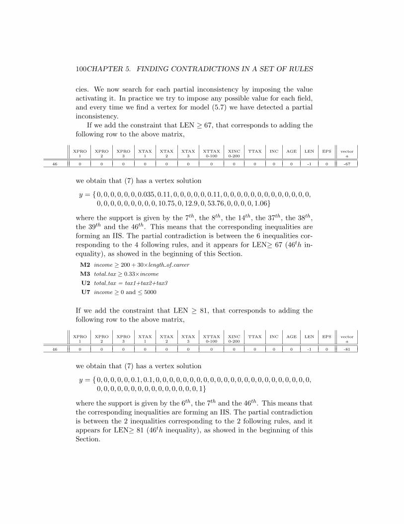
100CHAPTER 5. FINDING CONTRADICTIONS IN A SET OF RULES
cies. We now search for each partial inconsistency by imposing the valueactivating it. In practice we try to impose any possible value for each field,and every time we find a vertex for model (5.7) we have detected a partialinconsistency.
If we add the constraint that LEN ≥ 67, that corresponds to adding thefollowing row to the above matrix,
XPRO XPRO XPRO XTAX XTAX XTAX XTTAX XINC TTAX INC AGE LEN EPS vector1 2 3 1 2 3 0-100 0-200 a
46 0 0 0 0 0 0 0 0 0 0 0 -1 0 -67
we obtain that (7) has a vertex solution
y = {0, 0, 0, 0, 0, 0, 0.035, 0.11, 0, 0, 0, 0, 0, 0.11, 0, 0, 0, 0, 0, 0, 0, 0, 0, 0, 0, 0, 0,0, 0, 0, 0, 0, 0, 0, 0, 0, 10.75, 0, 12.9, 0, 53.76, 0, 0, 0, 0, 1.06}
where the support is given by the 7th, the 8th, the 14th, the 37th, the 38th,the 39th and the 46th. This means that the corresponding inequalities areforming an IIS. The partial contradiction is between the 6 inequalities cor-responding to the 4 following rules, and it appears for LEN≥ 67 (46th in-equality), as showed in the beginning of this Section.
M2 income ≥ 200 + 30×length of career
M3 total tax ≥ 0.33×income
U2 total tax = tax1+tax2+tax3
U7 income ≥ 0 and ≤ 5000
If we add the constraint that LEN ≥ 81, that corresponds to adding thefollowing row to the above matrix,
XPRO XPRO XPRO XTAX XTAX XTAX XTTAX XINC TTAX INC AGE LEN EPS vector1 2 3 1 2 3 0-100 0-200 a
46 0 0 0 0 0 0 0 0 0 0 0 -1 0 -81
we obtain that (7) has a vertex solution
y = {0, 0, 0, 0, 0, 0.1, 0.1, 0, 0, 0, 0, 0, 0, 0, 0, 0, 0, 0, 0, 0, 0, 0, 0, 0, 0, 0, 0, 0, 0, 0,0, 0, 0, 0, 0, 0, 0, 0, 0, 0, 0, 0, 0, 0, 0, 1}
where the support is given by the 6th, the 7th and the 46th. This means thatthe corresponding inequalities are forming an IIS. The partial contradictionis between the 2 inequalities corresponding to the 2 following rules, and itappears for LEN≥ 81 (46th inequality), as showed in the beginning of thisSection.
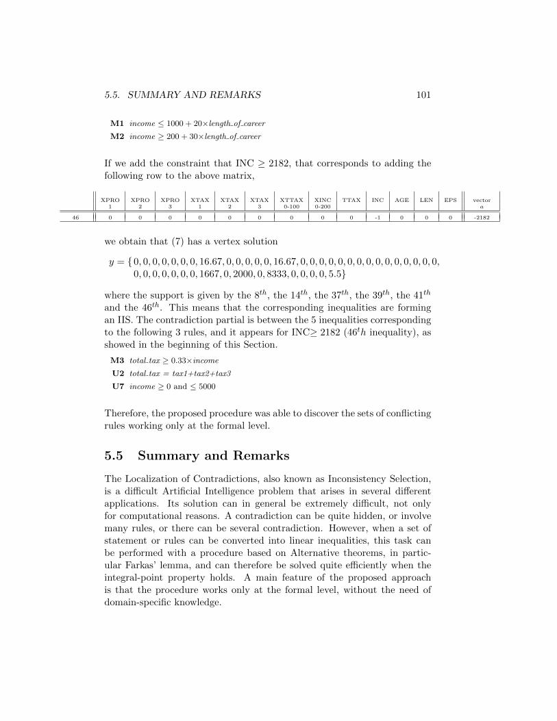
5.5. SUMMARY AND REMARKS 101
M1 income ≤ 1000 + 20×length of career
M2 income ≥ 200 + 30×length of career
If we add the constraint that INC ≥ 2182, that corresponds to adding thefollowing row to the above matrix,
XPRO XPRO XPRO XTAX XTAX XTAX XTTAX XINC TTAX INC AGE LEN EPS vector1 2 3 1 2 3 0-100 0-200 a
46 0 0 0 0 0 0 0 0 0 -1 0 0 0 -2182
we obtain that (7) has a vertex solution
y = {0, 0, 0, 0, 0, 0, 0, 16.67, 0, 0, 0, 0, 0, 16.67, 0, 0, 0, 0, 0, 0, 0, 0, 0, 0, 0, 0, 0, 0, 0,0, 0, 0, 0, 0, 0, 0, 1667, 0, 2000, 0, 8333, 0, 0, 0, 0, 5.5}
where the support is given by the 8th, the 14th, the 37th, the 39th, the 41th
and the 46th. This means that the corresponding inequalities are formingan IIS. The contradiction partial is between the 5 inequalities correspondingto the following 3 rules, and it appears for INC≥ 2182 (46th inequality), asshowed in the beginning of this Section.
M3 total tax ≥ 0.33×income
U2 total tax = tax1+tax2+tax3
U7 income ≥ 0 and ≤ 5000
Therefore, the proposed procedure was able to discover the sets of conflictingrules working only at the formal level.
5.5 Summary and Remarks
The Localization of Contradictions, also known as Inconsistency Selection,is a difficult Artificial Intelligence problem that arises in several differentapplications. Its solution can in general be extremely difficult, not onlyfor computational reasons. A contradiction can be quite hidden, or involvemany rules, or there can be several contradiction. However, when a set ofstatement or rules can be converted into linear inequalities, this task canbe performed with a procedure based on Alternative theorems, in partic-ular Farkas’ lemma, and can therefore be solved quite efficiently when theintegral-point property holds. A main feature of the proposed approachis that the procedure works only at the formal level, without the need ofdomain-specific knowledge.

102CHAPTER 5. FINDING CONTRADICTIONS IN A SET OF RULES
References
[1] G. Alexe, S. Alexe, P.L. Hammer and A. Kogan. Comprehensive vs. ComprehensibleClassifiers in Logical Analysis of Data. Discrete Applied Mathematics, vol. 156, no.6, 870-882, 2008.
[2] H. Almuallim and T.G. Dietterich. Learning Boolean Concepts in the Presence ofmany Irrelevant Features. Artificial Intelligence, vol. 69, no. 1, 279-306, 1994.
[3] E. Amaldi, M.E. Pfetsch and L. Trotter Jr.. Some structural and algorithmic prop-erties of the maximum feasible subsystem problem. Proceedings. of 10th IntegerProgramming and Combinatorial Optimization conference. Lecture Notes in Com-puter Science 1610, Springer, 45–59, 1999.
[4] M. Ayel and J.P. Laurent (eds.). Validation, Verification and Testing of Knowledge-Based Systems. John Wiley & Sons Ltd., Chichester, England, 1991.
[5] M. Bacharach. Matrix rounding problems. Management Science 12(9), 732-742,1966.
[6] M. Bacharach. Biproportional Matrices and Input-Output Change. Cambridge Uni-versity Press, Cambridge, UK, 2004.
[7] Banff Support Team. Functional Description of the Banff System for Edit andImputation System. Quality Assurance and Generalized Systems Section Tech. Rep.Statistics Canada, 2003.
[8] M. Bankier. Canadian Census Minimum change Donor imputation methodology. InProceedings of the Workshop on Data Editing, UN/ECE, Cardiff, United Kingdom,2000.
[9] M.S. Bazaraa, J.J. Jarvis, and H.D. Sherali. Linear Programming and NetworkFlows. John Wiley & Sons, second edition, New York, 1990.
[10] D. Bertsimas and J.N. Tsitsiklis. Introduction to Linear Optimization. AthenaScientific, Belmont, Massachusetts, 1997.
[11] G. Bianchi, R. Bruni and A. Reale. Open Source Integer Linear Programming Solversfor Error Localization in Numerical Data. In N. Torelli, et al. (eds.), Advances inTheoretical and Applied Statistics, Studies in Theoretical and Applied Statistics,Springer-Verlag Berlin Heidelberg, DOI 10.1007/978-3-642-35588-2 28, 2013.
103

104 REFERENCES
[12] G. Bianchi and R. Bruni. A Formal Procedure for Finding Contradictions into a Setof Rules. Applied Mathematical Sciences 6(126), 6253-6271, 2012.
[13] G. Bianchi, R. Bruni and A Reale. Balancing of Agricultural Census Data by UsingDiscrete Optimization. Optimization Letters, DOI 10.1007/s11590-013-0652-3, 2013.
[14] G. Bianchi, R. Bruni and A. Reale. Information Reconstruction via Discrete Opti-mization for Agricultural Census Data. Applied Mathematical Sciences Vol. 6(125),6241-6251, 2012.
[15] I.M. Bomze and M. Locatelli. Separable standard quadratic optimization problems.Optimization Letters 6, 857-866, 2012.
[16] N. Bourbaki. Topological vector spaces. Springer-Verlag, Berlin, Germany, 1987.
[17] S. Boyd and L. Vandenberghe. Convex Optimization. Cambridge University Press,Cambridge, UK, 2004.
[18] E. Boros, P.L. Hammer, T. Ibaraki and A. Kogan. Logical Analysis of NumericalData. Mathematical Programming, vol. 79, 163-190, 1997.
[19] E. Boros, P.L. Hammer, T. Ibaraki, A. Kogan, E. Mayoraz and I. Muchnik. AnImplementation of Logical Analysis of Data. IEEE Transactions on Knowledge andData Engineering, vol. 12, no. 2, 292-306, 2000.
[20] E. Boros, T. Horiyama, T. Ibaraki, K. Makino, and M. Yagiura. Finding EssentialAttributes from Binary Data. Annals of Mathematics and Artificial Intelligence, vol.39 no. 3, 223-257, 2003.
[21] E. Boros, Y. Crama, P.L. Hammer, T. Ibaraki, A. Kogan, and K. Makino. LogicalAnalysis of Data: Classification with Justification. Annals of Operations Research,vol. 188, 33-61, 2011.
[22] L. Breiman. Bagging predictors. Machine Learning, vol. 24, no. 2, 123-140, 1996.
[23] L. Breiman. Random Forests. Machine Learning, vol. 45, no. 1, 532, 2001.
[24] R. Bruni and A. Sassano. Error Detection and Correction in Large Scale DataCollecting. In Advances in Intelligent Data Analysis, Lecture Notes in ComputerScience 2189, Springer, 84-94, 2001.
[25] R. Bruni. Approximating Minimal Unsatisfiable Subformulae by means of AdaptiveCore Search. Discrete Applied Mathematics. Vol. 130(2), 85-100, 2003.
[26] R. Bruni. Discrete Models for Data Imputation. Discrete Applied Mathematics Vol.144/1, 59-69, 2004.
[27] R. Bruni. Error Correction for Massive Data Sets. Optimization Methods andSoftware, Vol. 20/2-3, 295-314, 2005.
[28] R. Bruni. On Exact Selection of Minimally Unsatisfiable Subformulae. Annals ofMathematics and Artificial Intelligence Vol. 43(1-4), 35-50, 2005.
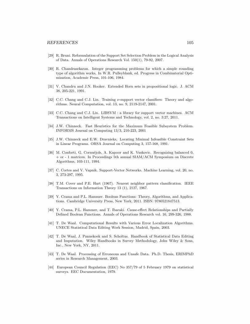
REFERENCES 105
[29] R. Bruni. Reformulation of the Support Set Selection Problem in the Logical Analysisof Data. Annals of Operations Research Vol. 150(1), 79-92, 2007.
[30] R. Chandrasekaran. Integer programming problems for which a simple roundingtype of algorithm works, In W.R. Pulleyblank, ed. Progress in Combinatorial Opti-mization, Academic Press, 101-106, 1984.
[31] V. Chandru and J.N. Hooker. Extended Horn sets in propositional logic. J. ACM38, 205-221, 1991.
[32] C.C. Chang and C.J. Lin. Training ν-support vector classifiers: Theory and algo-rithms. Neural Computation, vol. 13, no. 9, 2119-2147, 2001.
[33] C.C. Chang and C.J. Lin. LIBSVM : a library for support vector machines. ACMTransactions on Intelligent Systems and Technology, vol. 2, no. 3:27, 2011.
[34] J.W. Chinneck. Fast Heuristics for the Maximum Feasible Subsystem Problem.INFORMS Journal on Computing 13/3, 210-223, 2001
[35] J.W. Chinneck and E.W. Dravnieks, Locating Minimal Infeasible Constraint Setsin Linear Programs. ORSA Journal on Computing 3, 157-168, 1991.
[36] M. Conforti, G. Cornuejols, A. Kapoor and K. Vuskovic. Recognizing balanced 0,+ or - 1 matrices. In Proceedings 5th annual SIAM/ACM Symposium on DiscreteAlgorithms, 103-111, 1994.
[37] C. Cortes and V. Vapnik. Support-Vector Networks. Machine Learning, vol. 20, no.3, 273-297, 1995.
[38] T.M. Cover and P.E. Hart (1967). Nearest neighbor pattern classification. IEEETransactions on Information Theory 13 (1), 2127, 1967.
[39] Y. Crama and P.L. Hammer. Boolean Functions: Theory, Algorithms, and Applica-tions. Cambridge University Press, New York, 2011. ISBN: 9780521847513.
[40] Y. Crama, P.L. Hammer, and T. Ibaraki. Cause-effect Relationships and PartiallyDefined Boolean Functions. Annals of Operations Research vol. 16, 299-326, 1988.
[41] T. De Waal. Computational Results with Various Error Localization Algorithms.UNECE Statistical Data Editing Work Session, Madrid, Spain, 2003.
[42] T. De Waal, J. Pannekoek and S. Scholtus. Handbook of Statistical Data Editingand Imputation. Wiley Handbooks in Survey Methodology, John Wiley & Sons,Inc., New York, NY, 2011.
[43] T. De Waal. Processing of Erroneous and Unsafe Data. Ph.D. Thesis, ERIMPhDseries in Research Management, 2003.
[44] European Council Regulation (EEC) No 357/79 of 5 February 1979 on statisticalsurveys. EEC Documentation, 1979.
106 REFERENCES
[45] U.M. Fayyad, G. Piatetsky-Shapiro, P. Smyth and R. Uthurusamy (eds.) Advancesin Knowledge Discovery and Data Mining. AAAI Press / The MIT Press, MenloPark, CA, 1996.
[46] U.M. Fayyad and K.B. Irani. Multi-interval discretization of continuous-valued at-tributes for classification learning. Artificial Intelligence, vol.13, 1022-1027, 1993.
[47] I.P. Fellegi and I.P.D. Holt. A Systematic Approach to Automatic Edit and Impu-tation, Journal of the American Statistical Association 71, 17-35, 1976
[48] C. Forbes, M. Evans, N. Hastings, and B. Peacock, Statistical Distributions (fourthedition). Wiley series in Probability and Statistics, New York, 2010.
[49] A. Frank, A. Asuncion. UCI Machine Learning Repository[http://archive.ics.uci.edu/ml]. Irvine, CA: University of California, Schoolof Information and Computer Science, 2010.
[50] Y. Freund, Boosting a Weak Learning Algorithm by Majority. Information andComputation, vol. 121, no. 2, 256-285, 1995.
[51] W.A. Fuller. Measurement Error Models. Wiley Series in Probability and Statistics,John Wiley & Sons, Inc., New York, NY, 2006.
[52] M.R. Garey and D.S. Johnson. Computers and Intractability: A Guide to the Theoryof NP-Completeness. W.H. Freeman and Co, San Francisco, CA, 1979.
[53] R.S. Garfinkel, A.S. Kunnathur and G.E. Liepins. Optimal Imputation of ErroneousData: Categorical Data, General Edits. Operations Research 34, 744-751, 1986.
[54] R.S. Garfinkel, A.S. Kunnathur and G.E. Liepins. Error Localization for ErroneousData: Continuous Data, Linear Constraints. SIAM Journal on Scientific and Statis-tical Computing 9, 922-931, 1988.
[55] J. Gleeson and J. Ryan. Identifying Minimally Infeasible Subsystems of Inequalities.ORSA Journal on Computing 2/1, 61-63, 1990.
[56] O. Guieu and J.W. Chinneck. Analyzing Infeasible Mixed-Integer and Integer LinearPrograms. INFORMS Journal on Computing 11/1, 63-77, 1999.
[57] I. Guyon, N. Matic and V. Vapnik. Discovering Informative Patterns and DataCleaning.
[58] P.L. Hammer, A. Kogan, B. Simeone and S. Szedmak. Pareto-Optimal Patterns inLogical Analysis of Data. Discrete Applied Mathematics, vol. 144, no. 1-2, 79-102,2004.
[59] J. Han and M. Kamber. Data Mining: Concepts and Techniques. Elsevier, secondedition, 2006.
[60] D.J. Hand, H. Mannila and P. Smyth. Principles of Data Mining. MIT Press,London, 2001.

REFERENCES 107
[61] T. Hastie, R. Tibshirani and J. Friedman. The Elements of Statistical Learning:Data Mining, Inference and Prediction. Springer, New York, NY, 2001.
[62] T. Hastie, R. Tibshirani and J. Friedman. The Elements of Statistical Learning.Springer-Verlag, New York, Berlin, Heidelberg, 2002.
[63] F.S. Hillier and G.J. Lieberman. Introduction to Operations Research. McGraw-Hill,New York, NY, eighth edition, 2005.
[64] D.S. Hochbaum and J.G. Shanthikuma. Convex separable optimization is not muchharder than linear optimization. Journal of the ACM 37(4), 843-862, 1990.
[65] IBM: Ilog Cplex 12.1 Reference Manual. International Business Machines Corpora-tion, 2009.
[66] IBM: Ilog Concert Technology 12.1 Reference Manual. International Business Ma-chines Corporation, 2009.
[67] N. Jankowski, W. Duch, K Grabczewski (eds.) Meta-Learning in ComputationalIntelligence. Springer-Verlag, Berlin, 2011.
[68] M. Kantardzic. Data Mining: Concepts, Models, Methods, and Algorithms. JohnWiley & Sons Publishing, 2003.
[69] B. Kalantari, I. Lari, F. Ricca and B. Simeone. On the complexity of general matrixscaling and entropy minimization via the RAS algorithm. Mathematical Program-ming, Ser. A 112, 371401, 2008.
[70] W. Kløesgen and J.M. Zytkow (eds.). Handbook of Data Mining and KnowledgeDiscovery. Oxford University Press: Oxford, UK, 2002.
[71] L.E. Lyberg , P. Biemer, M. Collins, E.D. De Leeuw, C. Dippo, N. Schwarz andD. Trewin (eds.). Survey Measurement and Process Quality, Section C, post surveyprocessing and operations. John Wiley & Sons, Inc.: New York, NY, 1997.
[72] T. Menzies. Knowledge Maintenance: The State of the Art. Knowledge EngineeringReview, 14(1), 1-46, 1999.
[73] T.M. Mitchell, Machine Learning. McGraw-Hill, Singapore, 1997.
[74] A. Mucherino, P. Papajorgji and P.M. Pardalos. Data Mining in Agriculture.Springer: New York, NY, 2009.
[75] J.H. Myers and E.W. Forgy. The Development of numerical credit evaluation sys-tems. Journal of the American Statistical Association, Vol.58 Issue 303 (Sept) 799-806, 1963.
[76] G.L. Nemhauser and L.A. Wolsey. Integer and Combinatorial Optimization, J. Wiley& Sons, Inc., New York, NY, 1999.
[77] F.C. Pampel FC. Logistic regression: A primer. Sage University Papers Series onQuantitative Applications in the Social Sciences, 07-132. Thousand Oaks, CA: SagePublications, 2000.

108 REFERENCES
[78] C. Poirier. A Functional Evaluation of Edit and Imputation Tools. UN/ECE WorkSession on Statistical Data Editing, Working Paper n.12, Rome, Italy, 1999.
[79] W.H. Press, S.A. Teukolsky, W.T. Vetterling, and B.P. Flannery. Numerical Recipesin C: The Art of Scientific Computing, second edition. Cambridge University Press,1992.
[80] J.R. Quinlan. C4.5: Programs for Machine Learning. Morgan Kaufmann, San Mateo,CA, 1993.
[81] C.T. Ragsdale P.G. McKeown. On Solving the Continuous Data Editing Problem.Computers and Operations Research 23, 263-273, 1996.
[82] R. Ramakrishnan, J. Gehrke. Database Management Systems (third edition).McGraw-Hill: New York, NY, 2003.
[83] N. Rescher and R. Brandom. The Logic of Inconsistency. Basil Blackwell, Oxford,1980.
[84] J. Riera-Ledesma and J.J. Salazar-Gonzalez. New Algorithms for the Editing andImputation Problem. UNECE Statistical Data Editing Work Session, Madrid, Spain,2003.
[85] F. Rosenblatt. The Perceptron: A Probalistic Model For Information Storage AndOrganization In The Brain. Psychological Review 65 (6): 386-408, 1958.
[86] R.E. Schapire. The Strength of Weak Learnability. Machine Learning, vol. 5, no. 2,197-227, 1990.
[87] M.H. Schneider and S.A. Zenios. A comparative study of algorithms for matrixbalancing. Operations Research, 38(3), 439-455, 1990.
[88] A. Schrijver. Theory of Linear and Integer Programming. Wiley, New York, 1986.
[89] A. Schrijver. Combinatorial Optimization. Springer, Berlin, New York, 2003.
[90] M. Tamiz, S.J. Mardle and D.F. Jones. Detecting IIS in Infeasible Linear Programsusing Techniques from Goal Programming, Computers and Operations Research 23,113-191, 1996.
[91] V. Vapnik. Statistical Learning Theory. John Wiley and Sons, New York, 1998.
[92] G. Wei. Comparison Study of Genetic Algorithm and Evolutionary Programming.Proc. of the Third International Conference on Machine Learning and Cybernetics,1(1): 204-209, 2004.
[93] H.P. Williams. Model Building in Mathematical Programming. J.Wiley, Chichester,1993.
[94] W.E. Winkler. State of Statistical Data Editing and current Research Problems. InProceedings of the Workshop on Data Editing, UN/ECE, Rome, Italy, 1999.

REFERENCES 109
[95] W.L. Winston and M. Venkataramanan. Introduction to Mathematical Program-ming: Applications and Algorithms. Volume 1. Duxbury Press (fourth edition),Belmont, CA, 2002.
[96] D.H. Wolpert. The Lack of A Priori Distinctions Between Learning Algorithms.Neural Computation vol. 8, 1341-1390, 1996.
[97] Y. Yang and X. Liu. A re-examination of text categorization methods. AnnualACM Conference on Research and Development in Information Retrieval, 42-49,USA, 1999
[98] L.A.Zadeh. Fuzzy sets. Information and Control (8), 338-353, 1965.
[99] L.A.Zadeh. Calculus of fuzzy restrictions. In L. A. Zadeh, K.-S. Fu, K. Tanaka andM. Shimura (eds.), Fuzzy sets and Their Applications to Cognitive and DecisionProcesses. Academic Press, New York, 1975.
[100] G.P. Zhang. Neural Networks for Classification: a Survey. IEEE Transactions onSystems, Man, and Cybernetics. vol. 30, no. 4, 451-462, 2000.
[101] H. Zhang. The Optimality of Naive Bayes. FLAIRS2004 conference.
[102] H.-J. Zimmermann. Practical Applications of Fuzzy Technologies. Springer, 2000.


