General rights Copyright and moral rights for the publications made accessible in the public portal are retained by the authors and/or other copyright owners and it is a condition of accessing publications that users recognise and abide by the legal requirements associated with these rights.

• Users may download and print one copy of any publication from the public portal for the purpose of private study or research. • You may not further distribute the material or use it for any profit-making activity or commercial gain • You may freely distribute the URL identifying the publication in the public portal

If you believe that this document breaches copyright please contact us providing details, and we will remove access to the work immediately and investigate your claim.

Downloaded from orbit.dtu.dk on: May 09, 2018

Optimization of Thermo-mechanical Conditions in Friction Stir Welding

Tutum, Cem Celal; Hattel, Jesper Henri

Publication date:2010

Link back to DTU Orbit

Citation (APA):Tutum, C. C., & Hattel, J. H. (2010). Optimization of Thermo-mechanical Conditions in Friction Stir Welding. Kgs.Lyngby, Denmark: Technical University of Denmark (DTU).

Optimization of Thermo-mechanical

Conditions in Friction Stir Welding

by

Cem Celal Tutum

Ph.D. Thesis

Technical University of Denmark

Department of Mechanical Engineering

October, 2009

Optimization of Thermo-mechanical Conditions in Friction Stir WeldingCopyright ©, Cem Celal Tutum, 2009Process Modelling GroupDepartment of Mechanical EngineeringTechnical University of DenmarkKgs. Lyngby, Denmark

TM 02-09

ISBN 978-87-89502-89-2

To my mother

Preface

This work has been carried out at the Department of Mechanical Engineering (MEK),Technical University of Denmark (DTU), during the period 2006-2009. The work wassupervised by Professor Jesper H. Hattel (MEK), and co-supervised by Associate Profes-sor Henrik N. B. Schmidt (MEK) and Professor Martin P. Bendsøe, the Department ofMathematics (MAT), DTU.

I would like to express my sincere gratitude to Professor Hattel for his unfailingguidance and support throughout my studies, critical review of my work, and most im-portantly for his great patience and enthusiasm. I would like to thank Dr. Schmidt forproviding me irreplaceable inspiration with his state-of-the-art models and being morethan a co-supervisor. Special thanks to Prof. Bendsøe for taking intense academic inter-est in this study as well as providing valuable suggestions that improved the quality ofthe work.

I am also indebted to Jon Spangenberg and Petr Kotas; this work would not havebeen nalized without their help and encouragement. I would like to express my thanksto Kim Lau Nielsen and Anders Astrup Larsen together with other INNOJoint Projectmembers for their strong collaboration. Moreover, I would like to express my special grat-itude to Dr. Jesper Thorborg and Jens Ole Frandsen for always being ready for any kindof support. Vivek Chidambaram, Jokob Hilgert, Jacob Børby, Martin Asger Haugaard,José Blasques and Ramin Moslemian, thanks for being such companions on our journeysinto the wilds of Ph.D. studies.

Sincere thanks are due to the TopOpt (www.topopt.dtu.dk) research group membersfor their fruitful discussions and social activities spent together.

It was a privilege to meet Dr. Ivo Sbalzarini from ETH Zurich and have an opportu-nity to discuss on the evolutionary optimization and high performance computing. Mykeen appreciation goes to him for the inspiration he provided. My special thanks are alsodue to the Danish Center of Applied Mathematics and Mechanics (DCAMM) for oeringa wide range of courses that are given by distinguished researchers.

There are other people whom I owe quite a bit of inspiration. Ata Mu§an, Erol eno-cak, Haydar Livatyal and Ümit Sönmez are gratefully acknowledged.

I wish to express my cordial appreciation to my parents as well as Raik and Tülay,for their love, patience and encouragement. My mother Tülin, I devote this thesis to her.

v

Finally, my thanks go to Danish Government and DTU for their continuous nancialsupport and providing a nice working environment for this Ph.D. work during the threeyears.

Cem Celal TutumKgs. Lyngby, October 2009

vi

Abstract

The present thesis deals with the challenging multidisciplinary task of combining themanufacturing process of friction stir welding (FSW) with mathematical optimizationmethods in the search for optimal process parameters. The goals (objectives in optimiza-tion parlance) are process related in the sense that they describe or express when theprocess works in an optimal way or yields nal parts that are somehow optimal. Theseexpressions are denoted objective functions and the mathematical optimization algorithmis then searching for a set of the investigated process parameters (in optimization termsdenoted design variables) that will either minimize or maximize the objective functionsdepending on the problem at hand.

The FSW process which has been the subject of the optimization in this study is arelatively new welding process that was invented in 1991 by The Welding Institute (TWI),UK. In short, the process is solid-state, that is, no melting takes place, meaning that alot of the disadvantages normally associated with traditional fusing welding processes canbe avoided. In the FSW process a rotating tool is submerged into the two work piecesand due to frictional and plastic dissipation, the temperature is increased to an extendwhere the material is suciently softened to be stirred together, thereby forming a weld.The process is characterized by multiphysics involving solid material ow, heat transfer,thermal softening, recrystallization and the formation of residual stresses.

In the present work, several models for the FSW process have been applied. Initially,the thermal models were addressed since they in essence constitute the basis of all othermodels of FSW, be it microstructural, ow or residual stress models. Both analytical andnumerical models were used and combined with the Sequential Quadratic Programming(SQP) gradient-based optimization algorithm in order to nd the welding speed and theheat input that would yield a prescribed average temperature close to the solidus tem-perature under the tool, thereby expressing a condition which is favourable for the process.

Following this, several thermomechanical models for FSW in both ABAQUS and AN-SYS were developed. They were used for the analysis of the transient temperature andstress evolutions during welding and subsequent cooling, eventually leading to the residualstress state and reduced mechanical properties due to thermal softening. In one case, thesubsequent loading situation of a real FSW structure was also taken into account, thusmaking way for an integrated analysis of the welding process and the loading situationduring service of the welded part. Another case combined the predicted stresses with asubsequent uni-axial loading situation in which a damage evolution analysis was carriedout in order to predict the nal weld's load carrying capacity when subject to tensionperpendicular to the weld line.

vii

The thermomechanical models predicting residual stresses were also combined with anevolutionary optimization algorithm (NSGA-II) in the search for the optimal combinationof the process parameters that one essentially controls in practice, namely the weldingspeed and the rotational speed, which would minimize residual stresses and maximize thewelding speed divided by rotational speed (known as advancement per revolution andexpressing a desired feature of the process).

Finally, some more theoretical investigations regarding several well-known uncon-strained and constrained multi-objective-optimization (MOO) benchmark problems werecarried out. This was done in order to investigate some of the diculties that a multiobjective evolutionary algorithm may have to tackle. Specically, three elitist algorithms,i.e. the MOGA-II, the NSGA-II (the versions implemented in modeFRONTIER) and thecNSGA-II (custom NSGA-II implementation by the author in MATLAB with two versionsincluding the one with an extra Pareto-optimal set archieve strategy for post-processingpurposes), were employed for this purpose. The results (especially for the constrainedcase) show that the cNSGA-II shows a good performance for having both a convergedand a well-spread distribution of the Pareto-optimal set with less computational cost.

viii

Table of Contents

1 Introduction 1

1.1 Motivation of the work . . . . . . . . . . . . . . . . . . . . . . . . . . . . . 11.2 The Friction Stir Welding process . . . . . . . . . . . . . . . . . . . . . . . 21.3 Structure of the thesis . . . . . . . . . . . . . . . . . . . . . . . . . . . . . 7

2 Modeling 9

2.1 Thermal Modeling of FSW . . . . . . . . . . . . . . . . . . . . . . . . . . 92.1.1 Governing Equations . . . . . . . . . . . . . . . . . . . . . . . . . . 102.1.2 Analytical thermal models in FSW . . . . . . . . . . . . . . . . . . 11

2.1.2.1 Application of the Thin-Plate Solution in FSW . . . . . . 122.1.3 Prescribed heat source models in FSW . . . . . . . . . . . . . . . . 14

2.1.3.1 Steady-state Eulerian models with precribed heat source 172.1.3.2 Transient Lagrangian models with precribed heat source 20

2.1.4 Thermal-Pseudo-Mechanical model . . . . . . . . . . . . . . . . . . 222.2 Thermo-mechanical Modeling of FSW . . . . . . . . . . . . . . . . . . . . 24

2.2.1 Governing Equations . . . . . . . . . . . . . . . . . . . . . . . . . . 262.2.2 Analytical thermo-mechanical model . . . . . . . . . . . . . . . . . 292.2.3 Numerical thermo-mechanical models . . . . . . . . . . . . . . . . 31

2.2.3.1 Prescribed heat source-based residual stress models . . . 312.2.3.1.1 Case-A: . . . . . . . . . . . . . . . . . . . . . . . 332.2.3.1.2 Case-B: . . . . . . . . . . . . . . . . . . . . . . . 352.2.3.1.3 Case-C: . . . . . . . . . . . . . . . . . . . . . . . 37

2.2.3.2 TPM heat source-based residual stress models . . . . . . 382.2.4 Mechanical Properties of FS welds . . . . . . . . . . . . . . . . . . 41

2.2.4.1 Softening model . . . . . . . . . . . . . . . . . . . . . . . 422.3 Integrated modeling . . . . . . . . . . . . . . . . . . . . . . . . . . . . . . 47

2.3.1 Investigation of the service load performance of a friction stir weldedstructure by means of integrated modeling approach . . . . . . . . 47

2.3.2 Integrated modelling of residual stresses and damage evolution dur-ing in-service conditions of FSW joints . . . . . . . . . . . . . . . . 50

3 Optimization 57

3.1 An Overview on Optimization . . . . . . . . . . . . . . . . . . . . . . . . . 573.1.1 Classical Methods . . . . . . . . . . . . . . . . . . . . . . . . . . . 593.1.2 Evolutionary Algorithms . . . . . . . . . . . . . . . . . . . . . . . . 613.1.3 Hybrid Techniques . . . . . . . . . . . . . . . . . . . . . . . . . . . 61

3.2 Description of the Algorithms . . . . . . . . . . . . . . . . . . . . . . . . . 633.2.1 Sequential Quadratic Programming (SQP) . . . . . . . . . . . . . . 63

ix

3.2.2 Non-dominated Sorting Genetic Algorithm (NSGA-II) . . . . . . . 653.3 Optimization of the thermal models of FSW . . . . . . . . . . . . . . . . . 72

3.3.1 Optimization of the analytical thermal model . . . . . . . . . . . . 723.3.1.1 Derivation of the Closed Form Solution . . . . . . . . . . 733.3.1.2 Numerical Computation of the Average Temperature . . 733.3.1.3 Semi-Analytical Sensitivities . . . . . . . . . . . . . . . . 75

3.3.2 Optimization of the numerical (Eulerian) thermal model . . . . . . 753.4 Optimization of the thermo-mechanical models of FSW . . . . . . . . . . 77

3.4.1 Optimization of the residual stresses and production rate in FSW . 773.4.1.1 Problem Satement-1 . . . . . . . . . . . . . . . . . . . . . 793.4.1.2 Results of Problem Satement-1 . . . . . . . . . . . . . . . 803.4.1.3 Problem Satement-2 . . . . . . . . . . . . . . . . . . . . . 823.4.1.4 Results of Problem Satement-2 . . . . . . . . . . . . . . . 83

4 Summary of Appended Papers 85

4.1 PAPER-I . . . . . . . . . . . . . . . . . . . . . . . . . . . . . . . . . . . . 854.2 PAPER-II . . . . . . . . . . . . . . . . . . . . . . . . . . . . . . . . . . . . 854.3 PAPER-III . . . . . . . . . . . . . . . . . . . . . . . . . . . . . . . . . . . 864.4 PAPER-IV . . . . . . . . . . . . . . . . . . . . . . . . . . . . . . . . . . . 864.5 TECHNICAL REPORT-I . . . . . . . . . . . . . . . . . . . . . . . . . . . 864.6 TECHNICAL REPORT-II . . . . . . . . . . . . . . . . . . . . . . . . . . . 87

5 Conclusions and Future Work 89

5.1 Conclusions . . . . . . . . . . . . . . . . . . . . . . . . . . . . . . . . . . . 895.2 Future Work . . . . . . . . . . . . . . . . . . . . . . . . . . . . . . . . . . 90

Bibliography 93

Appendixes 105

A PAPER-I 107

B PAPER-II 117

C PAPER-III 129

D PAPER-IV 147

E TECHNICAL REPORT-I 159

F TECHNICAL REPORT-II 193

x

Chapter 1

Introduction

This Ph.D.thesis is the result of the project entitled "Thermo-mechanical Modelling andOptimization of Dynamic Process Conditions in Friction Stir Welding" which has beencarried out at the Process Modeling Group, Department of Mechanical Engineering, Tech-nical University of Denmark (DTU) in the period from July 2006 to October 2009.

1.1 Motivation of the work

The objective of this study is to investigate and control the thermomechanical conditions,mainly residual stresses and service-load conditions, in the friction stir welding (FSW)process by means of numerical modeling and optimization techniques, respectively. TheFSW process is not yet fully understood and since the 1990s, many theoretical/experi-mental investigations and EU supported industrial projects, e.g. JOIN-DMC and DEEP-WELD, have been carried out in order to get more knowledge about the many physicalaspects of the FSW process. FSW is used already in routine, as well as in critical ap-plications, for the joining of structural components mainly made of aluminium and itsalloys. However, further studies are still being carried out in order to obtain a morerobust "process window".

The eld of modelling FSW is broad ranging from models concerning e.g. microstruc-ture evolution, material ow, heat ow, heat generation, residual stresses, mechanicalloads (tool forces etc.) and strength of the joint. In order to get more insight into someof the fundamental mechanisms involved in the FSW process, the physical phenomenahave been divided into sub-systems, i.e. thermal and mechanical behavior, followed bythe integrated modeling approach combining coupled behavior of these two physical as-pects with the actual load case.

This Ph.D. study is part of the project named INNOJoint (Innovative Joining Pro-cesses Applying Integrated Modelling) a major research project at DTU Mechanical En-gineering which is an interdisciplinary project that focuses on determining appropriatewelding parameters as early as possible in the design process. Five professors and oneassociate professor from DTU, two postdocs, six PhD students and six multinationalcompanies, e.g. EADS (Airbus), BOSCH, Volvo, Danfoss, Grundfos and Danstir are alsoinvolved in the project.

The majority of the work carried out in the present Ph.D. project has been related to

1

computational models of dierent aspects of the FSW process. Especially, the thermalproles and transient/residual stresses evolved during and after welding, respectively, havebeen investigated numerically and compared with published experimental results. Thus,important information regarding the evolution of residual stresses which is a function ofthe main FSW process parameters, i.e. tool rotational speed and traverse welding speed,etc., is gathered by applying the general purpose nite element (FE) software ANSYS(Ansys Inc., 2007), ABAQUS (Dassault Systèmes, 2007) and COMSOL (COMSOL AB,2007). Following the modeling studies, numerical optimization routines, i.e. both classicaland evolutionary algorithms, have been used in order to nd optimum process parametersaiming at process-specic goals. These goals are formulated as single and multi-objectiveoptimization problems which need to be solved with appropriate numerical techniqueswhich utilize dierent solution strategies. For this purpose, the commercial programminglanguage MATLAB (The MathWorks Inc., 2007) and the multi-objective optimizationsoftware modeFRONTIER (ESTECO s.r.l., 2007), have been used.

1.2 The Friction Stir Welding process

Friction Stir Welding (FSW) is an ecient solid-state, i.e. without melting in the work-piece, joining technique that is intended to be used for joining of especially the aluminumalloys, besides dissimilar welds, which are dicult to weld with traditional welding tech-niques. Joining of large panels, which cannot be easily heat treated post weld to recovertemper characteristics, is another common interest for FSW to be preferred for industrialapplications besides its other benets. It was invented and experimentally proven byWayne Thomas and his colleagues at The Welding Institute, Cambridge, UK in Decem-ber 1991, and then TWI led for world-wide patent protection in December of that year(TWI, 1991; Wikipedia, 2009a; Bhadeshia, 2003).

In FSW, a cylindrical-shouldered tool, with a cylindrical/proled, threaded/unthreadedprobe (pin) is rotated at a constant speed and moved at a constant traverse rate in thejoint line between two pieces of sheet or plate material, which are butt welded togetheras shown in Figure 1.1. The parts have to be clamped rigidly onto a backing plate inorder to prevent the abutting joint faces from being forced apart but also to support thehigh plunging forces applied by the FSW machine head. The length of the pin is slightlyless than the required weld depth and the tool shoulder should be in direct contact withthe surface of the workpiece. The probe is submerged into the workpiece and then thetool is moved along the weld line with a tilt angle of 2-4 degress increasing the pressureunder the tool shoulder.

2

Figure 1.1: Schematic view of the FSW process [ref. PAPER-III] (Tutum et al., 2009).

Frictional heat is generated between the wear-resistant welding tool shoulder and pinon one side, and the material of the work pieces on the other. This heat, along with theheat generated by the plastic dissipation due to the mixing process, causes the stirredmaterials to soften without reaching the melting point (hence cited a solid-state process),allowing the traversing of the tool along the weld line in a plasticised tubular shaft ofmetal. As the pin is moved in the direction of welding, the leading face of the pin, oftenassisted by a special pin prole, forces plasticised material to the back of the pin whileapplying a substantial forging force to consolidate the weld metal. The welding of thematerial is facilitated by severe plastic deformation in the solid state, involving dynamicrecrystallization of the weld nugget (Murr et al., 1997).

(a) (b)

Figure 1.2: (a) An FSW weld between aluminium sheets (Nandan et al., 2008a). (b) Anactual tool, with a threaded-pin (Nandan et al., 2008a).

The solid-state nature of the FSW process, in combination with its unusual tool andasymmetric nature, results in a very characteristic microstructure. While some regionsare common to all forms of welding some are unique to the FSW process. While theterminology is varied the following is representative of the consensus.

3

The stir zone (also nugget, dynamically recrystallised zone), D in Fig. 1.3, is aregion of heavily deformed material that roughly corresponds to the location ofthe pin during welding. The grains within the stir zone are roughly equiaxed andoften an order of magnitude smaller than the grains in the parent material (Murret al., 1997). A unique feature of the stir zone is the common occurrence of severalconcentric rings which has been referred to as an onion-ring structure. The preciseorigin of these rings has not been rmly established, although variations in particlenumber density, grain size and texture have all been suggested.

The flow arm is on the upper surface of the weld and consists of material that isdragged by the shoulder from the retreating side of the weld, around the rear of thetool, and deposited on the advancing side of the weld.

The thermo-mechanically affected zone (TMAZ), C in Fig. 1.3, is situated oneither side of the stir zone. In this region the strain and temperature are lower thanin the stir zone and the eect of welding on the microstructure is correspondinglysmaller. Unlike the stir zone the microstructure is recognizably that of the parentmaterial, albeit signicantly deformed and rotated. Although the term TMAZtechnically refers to the entire deformed region it is often used to describe anyregion not already covered by the terms stir zone and ow arm.

The heat-affected zone (HAZ), B in Fig. 1.3, is common to all welding processes.As indicated by the name, this region is subjected to a thermal cycle but is notdeformed during welding. The temperatures are lower than those in the TMAZ butmay still have a signicant eect if the microstructure is thermally unstable. Infact, in age-hardened aluminium alloys this region commonly exhibits the poorestmechanical properties.

Figure 1.3: Schematic view of the weld zone with dierent regions (Frigaard and Grong Ø,2001).

Some of the advantages of FSW are improved mechanical properties of the welds, re-duced distortion and residual stresses, and benign environmental characteristics (Mishraand Ma, 2005). The requirement for lighter and load resistant structures, especially inaerospace and automotive industries, emphasizes the need for investigating the ecientchoice of the important process parameters that control the FSW welding procedure.

The solid-state nature of FSW immediately leads to several advantages over fusionwelding methods since any problems associated with cooling from the liquid phase areimmediately avoided. Issues such as porosity, segregation, solidication cracking and li-quation cracking are not an issue during FSW. In general, FSW has been found to producea low concentration of defects and is normally very tolerant to variations in parameters

4

and materials.

Nevertheless, FSW is associated with a number of unique defects. For example, insuf-cient weld temperatures, due to low rotational speeds or high traverse speeds, meaningthat the weld material is unable to accommodate the extensive deformation during weld-ing. This may result in long, tunnel-like defects running along the weld which may occuron the surface or subsurface. Low temperatures may also limit the forging action of thetool and thus reduce the continuity of the bond between the material from each side ofthe weld. The light contact between the material has given rise to the name kissing bond.This defect is particularly worrying since it is very dicult to detect using nondestructivemethods such as X-ray or ultrasonic testing. If the pin is not long enough or the tool risesout of the plate then the interface at the bottom of the weld may not be disrupted andforged by the tool, resulting in a lack-of-penetration defect. This is essentially a notch inthe material which can be a potential source of fatigue cracks.

A number of potential advantages of FSW over conventional fusion-welding processescan be summarized as below:

Good mechanical properties in the as welded condition

Improved safety due to the absence of toxic fumes or the spatter of molten material.

No consumables - conventional steel tools can weld over 1000 m of aluminium andno ller or gas shield is required for aluminium.

Easily automated on simple milling machines - lower setup costs and less training.

Can operate in all positions (horizontal, vertical, etc), as there is no weld pool.

Generally good weld appearance and minimal thickness under/over-matching, thusreducing the need for expensive machining after welding.

Low environmental impact.

However, some disadvantages of the process can be listed below:

Exit hole left when tool is withdrawn.

Large down forces required with heavy-duty clamping necessary to hold the platestogether.

Less exible than manual and arc processes (diculties with thickness variationsand non-linear welds).

Often slower traverse rate than some fusion welding techniques although this maybe oset if fewer welding passes are required.

The shipbuilding and marine industries are two of the rst industry sectors which haveadopted the FSW process for commercial applications. The process is suitable for the fol-lowing applications: panels for decks, sides, bulkheads and oors, aluminium extrusions,hulls and superstructures, helicopter landing platforms, oshore accommodation, marineand transport structures, masts and booms, e.g. for sailing boats and nally refrigerationplants.

5

At present the aerospace industry is welding prototype and production parts by FSW.Opportunities exist to weld skins to spars, ribs, and stringers for use in military and civil-ian aircraft. The Eclipse 500 aircraft, in which ' 60% of the rivets are replaced byfriction stir welding, is now in production. This oers signicant advantages comparedto riveting and machining from solid, such as reduced manufacturing costs and weightsavings. Longitudinal butt welds in Al alloy fuel tanks for space vehicles have been fric-tion stir welded and successfully used. The process could also be used to increase the sizeof commercially available sheets by welding them before forming. The FSW process cantherefore be considered for: wings, fuselages, empennages, cryogenic fuel tanks for spacevehicles, aviation fuel tanks, external throw away tanks for military aircraft, military andscientic rockets, repair of faulty MIG welds, various primary and secondary structuralcomponents.

Several examples on the commercial production of high speed trains made from alu-minium extrusions which may be joined by FSW are given in Skillingberg and Green(2007); TWI (1991). Applications include: high speed trains, rolling stock of railways,underground carriages, trams, railway tankers and goods wagons as well as containerbodies.

The FSW process is currently also being used commercially in the automotive indus-try. Existing and potential applications include: engine and chassis cradles, wheel rims,attachments to hydroformed tubes, tailored blanks, e.g. welding of dierent sheet thick-nesses, space frames, e.g. welding extruded tubes to cast nodes, truck bodies, tail liftsfor lorries, mobile cranes, armour plate vehicles, fuel tankers, caravans, buses and aireldtransportation vehicles, motorcycle and bicycle frames, articulated lifts and personnel,bridges, skips, repair of aluminium cars, magnesium and magnesium/aluminium joints.

Finally, FSW can also be considered for other applications, such as electric motorhousings (in production), refrigeration panels, cooking equipment and kitchens, whitegoods, gas tanks and gas cylinders and connecting of aluminium or copper coils in rollingmills.

6

1.3 Structure of the thesis

The thesis constitutes of 5 chapters followed by 4 appended papers and 2 technical reports.

In Chapter 1, the motivation of the work has been given with an overview of the needsfor investigations in the FSW process followed by some examples of industrial applications.

Chapter 2, is overall speaking devoted to modeling of the FSW process and it is ini-tiated by the thermal modelling and then combined with the mechanical modeling wheretransient thermal as well as residual stresses together with a real-world service load ap-plication, is presented.

Analytical models, precribed heat source models and the thermal-pseudo-mechanicalheat source model constitute the backbone of the thermal modeling section, which isalso the main driver for the mechanical models presented in the subsequent section ofthe modeling chapter. Except for the steady-state analytical (thin plate) thermal modelpresented in PAPER-I, the rest of the thermal models are dealing with both steady-stateand transient cases. PAPER-I also includes a comparison of a relatively simple analyticalsolution with a more complex 2-D Eulerian model in order to be used for obtaining anaverage temperature under the tool shoulder.

The mechanical modeling section is mainly based on PAPERs-II-III and IV althoughsome of them are also optimization oriented. An overview of the governing equations forthe thermo-mechanical modeling and the evolution of residual stresses for welding ap-plications are given rst and then an analytical thermo-elastic solution for the movingline-type heat source is presented in order to initiate the discussions for the fundamen-tal issues in thermo-mechanics. Next, numerical nite element models for the residualstress calculations investigating the dierent clamping conditions and dierent levels oftemperature dependency of the yield stress, using prescribed and TPM-heat source basedthermal models (which are implemented using commercial software, i.e. ABAQUS andANSYS) are given in detail. Following these numerical models, mechanical properties offriction stir welded structures is presented briey with an accompanying softening (dis-solution) model.

As a nal topic of the modeling chapter the integrated modeling approach, applied toFSW for simulation of the service-load performance of a welded structure and a damageevolution in a FSW joint specimen during in-service conditions, is presented.

Chapter 3, considers mainly optimization studies aiming at process-specic goals orsuccess criteria satisfying limitations related to the production. A brief overview on op-timization methodologies is given initially, including deterministic traditional techniquesand nature inspired undeterministic approaches (i.e. genetic algorithms) as well as hybridmethodolgies aiming at combining the advantages of both strategies for multi-objectiveoptimization cases in particular. A brief description of the algorithms, i.e. the Sequen-tial Quadratic Programming (SQP) as the classical gradient based technique and theNon-dominated Sorting Genetic Algorithm (NSGA-II) as the multi-objective evolution-ary algorithm, is given. Following these introduction sections, two optimization problemsbased on thermal and thermo-mechanical (residual stress) models, are presented in detail.

7

The rst deals with both analytical and numerical thermal models combined withthe Sequential Quadratic Programming (SQP) gradient-based optimization algorithm inorder to nd the welding speed and the heat input that would yield a prescribed averagetemperature close to the solidus temperature under the tool, thereby expressing a condi-tion which is favourable for the process.

The second applies the thermomechanical models predicting residual stresses in com-bination with the evolutionary optimization algorithm (NSGA-II) in the search for theoptimal combination of the process parameters of welding speed and rotational speed,which would minimize residual stresses and maximize the welding speed divided by rota-tional speed (known as advancement per revolution and expressing a desired feature ofthe process).

Chapter 4 is dedicated to summary of appended 4 articles and 2 technical reports.

Chapter 5 presentes the conclusions of the thesis and suggestions for future researchdirections.

Finally, in the two technical reports, focus is put on the well-known benchmark prob-lems for multi-objective optimization with and without constraints. In these, a com-parison of three algorithms, i.e. the MOGA-II and the NSGA-II in the commercialmulti-objective optimization software modeFRONTIER together with the custom imple-mentation by the author of the NSGA-II in MATLAB, is carried out.

8

Chapter 2

Modeling

This chapter focuses on the thermal and thermo-mechanical modeling studies in the FSWprocess ranging from 2-D analytical models to 3-D numerical models. First, thermal mod-els which are mainly the driving force for the thermo-mechanical models, i.e. residualstress models, are presented in detail. Following that, thermo-mechanical models in-cluding residual stress calculations and integrated modeling studies, i.e. combining withservice load performance of the welded structure, are presented.

2.1 Thermal Modeling of FSW

In the FSW process shown schematically in Fig. 1.1, heat is generated by friction and bythe plastic deformation that occur between the tool and the work piece. The heat owsinto the work piece as well as the tool. The amount of heat that is conducted into thework piece inuences the quality of the weld, as well as the distortion and residual stressesin the work piece. For example, insucient heat generation could lead to failure of thetool pin since the work piece material is not soft enough. Therefore, understanding theheat ow aspects of the FSW process is extremely important, not only for understandingthe physical phenomena but also for improving the process eciency in order to obtaingood weld properties.

Thermal modelling has since the late nineties been a central part of modelling of FSWin general (Schmidt and Hattel, 2008a). One of the reasons for this is that many of theproperties of the nal weld are directly a function of the thermal history which the work-piece has been exposed to. Secondly, the FSW process itself is highly aected by the heatgeneration and heat ow and thirdly, from a modelling viewpoint, thermal modelling ofFSW can be considered the basis of all other models of the process, be it microstructural,Computational Fluid Mechanics (CFD) or Computational Solid Mechanics (CSM) mod-els.

In the FSW process the welding parameters, i.e. tool rotational speed, traverse speed,etc., are all chosen such that the softening of the workpiece material enables the me-chanical deformation and material ow. However, unlike many other thermomechanicalprocesses, the mechanisms of FSW are fully coupled meaning that the heat generation isrelated to material ow and frictional/contact conditions and vice versa. Thus, in theorya thermal model alone cannot predict the temperature distribution/history without apre-knowledge about the heat generation, since the fundamental mechanisms of FSW are

9

not part of a pure thermal model. For this reason, several analytical expressions havebeen given in literature for the heat generation for a given weld as a function of toolgeometry and welding parameters, e.g. tool radius and rotational speed (Schmidt andHattel, 2008a; Hattel et al., 2008).

2.1.1 Governing Equations

All thermal models, independent of their complexity, rely on the solution of the classi-cal heat conduction equation, Eq. (2.1), which is a scalar partial dierential equation(PDE) in mathematics parlance (Betounes, 1998; Carslaw and Jaeger, 1959). This time-dependent problem can be solved equivalently in both Lagrangian and Eulerian referenceframes with an appropriate set of initial and boundary conditions. In the former case,the thermal eld is described with respect to a xed coordinate system whereas in thelatter case the coordinate system moves with the heat source as schematically shown inFigure 2.1. The temperature change in a region over time is formulated in the Lagrangianreference frame as

ρcp∂T

∂t= ∇(k∇T ) + qvol (2.1)

where ρ denotes the material density(kgm3

), cp the specic heat capacity

(J

kgK

), T the

temperature eld (K), k the thermal conductivity(WmK

), and qvol the volumetric heat

source term(Wm3

). Under the assumption of constant thermal conductivity, independent

of temperature, Eq. (2.1) can be reformulated,

∂T

∂t=

k

ρcp∇2T +

qvolρcp

(2.2)

where the constant term[kρcp

]is called the thermal diusivity of the material which

is a measure of how fast heat is conducted in a solid (Carslaw and Jaeger, 1959; Lindgren,2007).

In case of describing the heat ow in a Eulerian reference frame, a convective term isadded to Eq. (2.1) as given by

ρcp∂T

∂t= ∇(k∇T ) + qvol − ρcpu∇T (2.3)

where u is the velocity eld vector which can contain the tool welding velocity as wellas the material ow eld around the tool probe, i.e. in the shear layer.

If transient eects are negligible, the time-dependent term, i.e. ∂T∂t vanishes and Eq.

(2.1) in the Lagrangian reference frame is reduced to

0 = ∇(k∇T ) + qvol (2.4)

and correspondingly in the Eulerian reference frame Eq. (2.5) is obtained.

10

Figure 2.1: Schematic view of the Lagrangian and the Eulerian reference frames.

0 = ∇(k∇T ) + qvol − ρcpu∇T (2.5)

Although the use of the former approach is quite common, the latter can take ad-vantage of the steady state conditions that may exist with respect to the moving heatsource (Lindgren, 2007). These formulations are summed up in tabular form to give anoverview in Table 2.1. Besides some numerical applications of the latter, it also results inimportant analytical formulations to be presented in detail in the following section. Thecombination of the choice of reference frame and degree of enmeshed modeling level oersa huge range of possibilities, and the "correct" choice depends on the objective of eachmodel. As an example, a residual stress model would need a temperature eld comingfrom a transient Lagrangian thermal model (Schmidt and Hattel, 2008a).

Table 2.1: Governing (heat conduction) equations in thermal models with respect todierent reference frames and time domains [ref. PAPER-IV] (Hattel et al., 2008)

Reference Frame Transient Steady-state

Lagrangian ρcp∂T∂t = ∇(k∇T ) + qvol 0 = ∇(k∇T ) + qvol

Eulerian ρcp∂T∂t = ∇(k∇T ) + qvol − ρcpu∇T 0 = ∇(k∇T ) + qvol − ρcpu∇T

2.1.2 Analytical thermal models in FSW

An accurate solution of the complete heat conduction equation considering heat transferby both conduction and convection is complicated. As a rst step, it is often useful todiscuss a simplied solution considering only conduction heat transfer. Following that,other simplications can be sorted as using constant (temperature independent) materialproperties, i.e. k, ρ and cp, simplications in the heat sources (Gaussian distributionof the heat source, double elipsoid heat source as well as point and line heat sources),

11

time dependence (assuming steady-state conditions) and boundary conditions (innite orsemi-innite domains). These simplications are attractive since analytical solutions canbe obtained for the heat conduction equation in many situations and these solutions canprovide interesting insight about the welding process (Feng, 2005). In the next section,an analytical model particularly applicable for FSW process will be described in detailand it will constitute the basis for Section 3.3.1, relating closely to PAPER-I (Tutum et al.,2007).

2.1.2.1 Application of the Thin-Plate Solution in FSW

A schematic view of a line-type heat source moving with a constant speed along a linein an innitely extended plate is shown in Fig. 2.2a. The temperature eld is governedby the same heat conduction partial dierential equation, including the convection term,as given in Eq. (2.3). The closed form solution can be obtained under quasi-steady stateassumptions as given by Eq. (2.6) (Rosenthal, 1946),

T =(Qtot2πkd

)e−uweldξ

2a K0

(uweld2a

r)

+ T0 (2.6)

where (Qtot/d) denes the heat input per unit thickness, ξ denotes the moving coordinateaxis (r =

√ξ2 + y2), a is the heat diusivity, K0 denotes the Modied Bessel Function

of the second kind and zeroth order and T0 denes the ambient temperature.

Fig. 2.2b shows the resulting temperature proles along the welding axis at dierentdistances, i.e. y = 0, 5, 10, 15 and 20 cm away from the joint line, while the heat sourceis passing by x = 0 m. Notice the mathematical singularity of innite temperature atthe location of the heat source, which of course is not possible in real FSW applicationswhere the solidus temperature is the limit for peak temperatures.

(a) (b)

Figure 2.2: (a) Schematic view of a line-type heat source moving along the joint line ofthe work piece [ref. PAPER-I] (Tutum et al., 2007). (b) Temperature prole along x-axisat dierent y-points (Tutum and Hattel, 2008).

Fig. 2.3a shows the thermal eld where only the 1.2 m x 1 m region surrounding theheat source is considered. Notice from Fig. 2.3b that the analytical model does not seethe eects of the boundary conditions because of the innitely large domain description,

12

while this is not the case for the numerical model having a nite domain, see Section2.1.3.1, Fig. 2.8.

(a) (b)

Figure 2.3: (a) Temperature eld on a 3 mm-thick plate (Tutum and Hattel, 2008). (b)Contour plot of the temperature eld (Tutum and Hattel, 2008).

It should be mentioned that a modied version of this solution given by Eq. (2.6) isused later in Chapter 3 for obtaining optimal values of the heat input and the weldingvelocity. Details about this are given in Section 3.3.1.

The Rosenthal solutions described above have been widely used, especially in the earlymodelling of FSW. In Gould and Feng (1998) and McClure et al. (1998) the 3D Rosenthalsolution is used to develop a circular heat source resembling the shoulder of the tool byplacing sources in a ring around the tool center and integrating to obtain the full temper-ature eld. The heat is assumed to be generated by Coulomb friction between the tooland the workpiece, i.e. δ = 0, see Eq. (2.7) for denition. Russell and Shercli (1999)presented an analytical model using the Rosenthal point heat source solution as a thermalmodel in order to be used as an input for the subsequent microstructure (softening) modelbased on the method of Myhr and Grong (1991a,b), which has proven to be sucientlyaccurate for FSW of many Al-alloys. The softening of the material (dissolution of theprecipitates in the alloy) is mainly governed by the thermal cycles, which are integratedover time, rather than the peak temparatures. Fonda and Lambrakos (2002) presented amore detailed analytical model based on the 3D Rosenthal solution involving nite platethickness and distribution of several point heat sources around the tool. By using aninverse modelling technique, the temperature eld described by the peak temperatures,is adjusted by scaling the power of the heat sources with respect to the hardness measure-ments. Vilaça et al. (2005) developed an analytical thermal model for 2D and 3D casesusing modied Rosenthal solutions, again based on a reverse engineering approach, i.e.modifying the process parameters iteratively along with thermal measurements, enablingsimulation of the asymmetric temperature prole induced by the tool rotations. Finally,Larsen et al. (2009) used the 2D Rosenthal solution to optimize a FSW thermal model byusing space mapping and manifold mapping in which a coarse model is used along witha ne FE-based model to be optimized.

13

2.1.3 Prescribed heat source models in FSW

In most pure thermal models of FSW, the heat generation from both frictional and plasticdissipation is modelled via a surface ux boundary condition at the tool/matrix interface.The main unknown parameters in these surface ux expressions are either the frictioncoecient under the assumption of sliding and the material yield shear stress under theassumption of sticking.

Along this line, Schmidt and Hattel (2004) have proposed the following generallyadopted equation for the total heat generation [W ],

Qtotal = δQsticking + (1− δ)Qsliding,

=23πω [δτyield + (1− δ)µp]

[(R3shoulder −R3

probe

)(1− tanα) +R3

probe + 3R2probeH

](2.7)

where δ is the dimensionless slip rate between the tool and the workpiece (1 for fullsticking and 0 for full sliding).

Figure 2.4: Schematic view of analytical tool geometry (including conical shoulder andcylindrical probe and heat generation contributions from shoulder Q1, probe side Q2 andprobe tip Q3 (Schmidt and Hattel, 2004, 2005).

However, when implementing this into a numerical model using a position dependentsurface ux [W/m2], it is typically used on the following form (Schmidt and Hattel, 2005),

qtotal = γτfriction + (ωr − γ) τyield,= ωr [δτyield + (1− δ)µp] (2.8)

which in fact is the basis for deriving equation, Eq. (2.7). Furthermore, when com-bining Eq. (2.7) and (2.8) and then assuming the simple tool geometry of a at shoulder,one obtains the following well-known expression for the heat generation (Schmidt andHattel, 2005),

qtotal =3Qtotalr

2πR3shoulder

(2.9)

which can be applied as a radius dependent surface ux in the model, under the as-sumption of a constant contact condition close to sliding or in cases of sticking where the

14

shear layer is very thin.

From Eq. (2.9) it can be seen that Qtotal can be considered an input parameter inthe same manner as the friction coecient, the pressure and the material's yield shearstress in Eq. (2.7). However, it should be mentioned that having Qtotal as part of theinput parameters for the model in some situations could conict with the very objectivefor thermal modelling of FSW. This is especially the case when the model should predicttemperatures for conditions not supported by measurements of the heat input Qtotal. Inthese cases it is not straightforward to predict or simulate the eect of e.g. a change inwelding or rotational speed, because the total heat generation Qtotal is a function of thesechanges in parameters and hence can be considered an internal function of the FSW pro-cess; unlike other welding process, e.g. TIG where the heat input is controlled externally.

This dilemma can obviously be overcome by supporting the thermal model with athermo-mechanical CSM or CFD based model which "includes" the underlying physicsof the process, namely the material ow producing heat generation by plastic dissipationin the shear layer and frictional contact at the tool/workpiece. As being pretty obviousfrom the later section on thermo-mechanical modeling, the eorts for such simulations arehighly demanding from both a computational and a human resource point of view, thusleaving pure thermal modelling of FSW as a valuable "simple" alternative for simulationof heat ow having in mind the limitation of such models, which as earlier mentionedprimarily lie in the evaluation of Qtotal.

Having said that, it should be noted that the most utilized procedure for evaluatingQtotal typically is to rely on experimental ndings by simply performing the actual weldsand measuring Qtotal with a dynamometer, and thereby accepting the inherent limitationof the resulting thermal model to predicting only temperatures for a known total heatgeneration.

Since the prescribing of the heat generation is the most single important parameterin thermal models of FSW, Schmidt and Hattel (2005) proposed a classication of dif-ferent heat sources as shown in Fig. 2.5. One characteristic in this classication is how"detailed" the tool heat generation is resolved. Three levels were evaluated, i.e. i) includ-ing shoulder heat generation, without probe heat generation, ii) including shoulder andprobe heat generation, with probe material and iii) shoulder and probe heat generationbut without probe material.

A second characteristic was whether the convective contribution due to the materialow in the shear layer was taken into account. Two extreme contact conditions wereevaluated, i.e. full sliding and full sticking. In the case of sliding the heat was applied asa surface ux and in the case of sticking the heat was applied as a volume ux in a shearlayer. This shear layer was prescribed analytically assuming a uniform thickness with alinear velocity prole ramped between the tool velocity at the contact interface and thewelding velocity outside the shear layer.

15

Figure 2.5: Schematic view of conguration of six cases of prescribing the heat generationin FSW: the left-hand column is for sliding condition and the right-hand column forsticking condition; the rst row shows no probe heat generation, the second row is withprobe heat generation, and the third row is for the probe volume removed, and heatgeneration in the shear layer (Schmidt and Hattel, 2005).

It was concluded that for analysing the temperature eld in the volume under thetool, special attention should be paid to the heat generation and how the material "ows"around the tool probe. The main eect of including the probe in the thermal model isto change the material properties to those of the tool; secondly, rotating the probe andmodelling the shear layer around it such that it resembles a ow model.

One new procedure to obtain the heat generation is to couple the traditional ana-lytical expression for the heat generation with a constraint based on experimental orphenomenological considerations. It is well-known from the constitutive behaviour of asolid (representative for those alloys used in FSW), that the yield stress dramaticallydecreases once the temperature approaches the solidus temperature. Above the solidustemperature, the material acts as a uid. As a consequence, the material close to thetool/matrix interface will reduce its heat generation to negligible values if exceeding thesolidus temperature subsequently reducing the temperature level, allowing the materialto recover its strength. A selfstabilizing eect will thus establish at a temperature levelaround the solidus temperature, hence this could be used as an average temperature con-straint in a pure thermal model. This is what is done in the thermal model by Tutumet al. (2007) [ref. PAPER-I], where the heat generation in FSW of AA2024 is controlled byusing an optimization scheme such that an average temperature of 500 °C at the tool/-workpiece interface is obtained. This procedure has given promising results for obtainingtemperature elds without prior knowledge regarding Qtotal; in fact this is an outputof the optimization analysis. A more thorough description of this approach is given inSection 3.3.

16

2.1.3.1 Steady-state Eulerian models with precribed heat source

Modeling the whole welding process, i.e. plunge, dwell and pull out periods, holds somenotable complexities. In order to reduce the computational cost regarding the movingheat source, meanwhile preserving the applicability, only the welding period is taken intoaccount and a moving coordinate system which is located on the heat source is applied.Eq. (2.2) describes the heat transfer in the plate in general and it is modied into Eq.(2.5) as described in Section 2.1.1. The traverse motion of the tool is modeled by prescrib-ing a material ow through the rectangular plate region. Due to this ow prescription,the equation includes a convective term in addition to the conductive term. If the heatow problem involves material ow, the Eulerian formulation is often advantageous. InFig. 2.6, the boundary conditions are described for the steady state Eulerian model inthe simulation tool COMSOL.

Figure 2.6: Schematic view of the numerical model with boundary conditions [ref.PAPER-I] (Tutum et al., 2007).

The circle with a radius of Rsh=10 mm, in the middle of the rectangular region, rep-resents the tool shoulder where the stationary and uniform heat source is applied as avolume ux in the shear layer. The tool is stationary while the material ows through itwith a velocity of uweld in the opposite welding direction, in Fig. 2.6. The room temper-ature (20 °C) is dened at the right edge of the rectangular region. The heat ux on theleft edge of the plate region, where the aluminum leaves the computational domain, isdominated by convection. On the upper and lower edges of the plate boundaries, thermalinsulation is enforced.

A schematic view of the applied volume heat ux as shown in Fig. 2.7 , is given by,

qtotal =3Qtotalr

2πR3shoulderd

(2.10)

where Qtot is the total heat input, d denotes the thickness of the actual shear layerunder consideration and r is the radius originating at the center of the tool. This volumeheat ux corresponds to a surface heat ux from the tool shoulder (without the toolprobe) (Schmidt and Hattel, 2005), distributed through the plate thickness under theassumption of 2D heat ow. This corresponds to Case 1b in Fig. 2.5 for a thin plate.

17

Figure 2.7: Schematic view of tool geometry with applied linear heat source on toolshoulder in 2D thermal model [ref. PAPER-I] (Tutum et al., 2007).

Fig. 2.8 shows the contour plot of the resulting temperature eld of the model(isotherms in 50 K increments). The modeling includes aluminum properties for theworkpiece material for a 3 mm-thick plate. The welding speed is 2 mm/s. Notice thatthe maximum temperature is around 800 K, which is a result of having higher temper-atures than a desired average temperature over the shoulder area of 500 °C. This is notphysically possible since the solidus temperature, Tsol , for this case was chosen to be 500°C (' 773 K); however this is a result of the use of a simple heat source model.

Figure 2.8: Contour plot of the temperature eld. Increment between isotherms is 50 K[ref. PAPER-I] (Tutum et al., 2007).

This 2D Eulerian thermal model can be extended into the following 3D Eulerian ther-mal model, shown schematically in Fig. 2.9, including the prescribed material ow underthe tool shoulder (without probe) and the steel backing plate which absorbs the heatfrom the aluminum workpiece. The convective heat transfer induced by the material owwhich is a function of the contact condition, i.e. sliding, sticking or partial sliding/stick-ing, aects the local temperature distribution close to the tool/matrix interface. Somerenements of the shoulder heat source are particularly examined for the two extremecontact conditions, i.e. full sliding and full sticking, further discussions are given bySchmidt and Hattel (2005), see Fig. 2.5.

Case-1a considers the full sliding contact condition at the tool shoulder/matrix inter-face where the contact shear stress described by Coulomb's law (τcontact = τfriction = µP )is less than the material yield shear stress, thus resulting in no workpiece deformation.The heat source is dened as a surface heat ux acting on the top surface of the thin

18

(a) (b)

Figure 2.9: (a) Geometry of the 3D Eulerian thermal model with boundary conditions(case 1a and 1b). (b) Closer view of the shear layer and prescribed velocity eld (inspiredby Schmidt and Hattel (2005)).

cylindrical volume representing the shear layer shown in Figs. 2.10a and 2.10b. As dis-cussed before in Section 2.1.3, the surface heat ux contributes to the steady-state heatconduction equation, Eq. (2.5), as a boundary condition. Case-1b takes the full stickingcontact condition into account at the tool shoulder/matrix interface where the frictionshear stress is higher than the matrix yield shear stress denoting that the matrix is de-formed with the same rate as the tool rotational speed (a segment at the top surfaceof the matrix sticks to the tool surface). Since the base matrix is stationary relative tothe shoulder/matrix interface, a deformation layer is established. The eect of this layercan be visualized using a ramping factor which scales the velocity of the segments insidethe volume in the vertical direction as seen in Fig. 2.9b. In this case the heat source isapplied in the thin shear layer as a volumetric heat ux, qvol in Eq. (2.5). The resultingthermal eld for this Case-1b is shown in Fig. 2.10a and the asymmetric temperaturedistribution around the shear layer can be seen in Fig. 2.10b.

(a) (b)

Figure 2.10: (a) Temperature eld (Case-1b) (Tutum, 2007b). (b) A cross-sectionalview of the temperature eld around the shear layer, notice the asymmetric temperaturedistribution due to the material ow in the shear layer (Tutum, 2007b).

19

The dierence in the temperature distribution between the two cases of 1a and 1b isnoticable from the thermal proles given in Figs. 2.11a and 2.11b. As can be seen it isapproximately 15 °C at a distance from the center equal to the half of the tool shoulderradius, particularly in the retreating side.

(a) (b)

Figure 2.11: (a) Comparison of the thermal proles in Case-1a (symmetric) and Case-1b(asymmetric) along the transverse direction through the center of the heat source at thetop surface (Tutum, 2007b). (b) Closer view of the thermal proles in the diameter ofthe tool shoulder (Tutum, 2007b).

2.1.3.2 Transient Lagrangian models with precribed heat source

Steady-state Eulerian thermal models with prescribed heat sources with respect to dif-ferent contact conditions have been described in the previous section. However, in orderto take the transient eects into account, preparing a Lagrangian model is more ecientcompared to a transient Eulerian model, as discussed in Section 2.1.1.

The model presented below represents the welding of two at plates by consideringthe bead on plate. Due to symmetry assumptions, i.e. neglecting the asymmetric heatsource caused by the asymmetric shear layer formation, only one of the plates is modeled.The dimension of the workpiece is 600 mm x 100 mm x 3 mm. Due to the very lowcontribution to the heat generation coming from the tool pin, only the tool shoulder isconsidered in the heat source and it is modelled as a surface heat ux moving along thejoint line on the top surface (1.5 mm oset from the middle section) of the shell niteelement model. The diameter of the tool shoulder is 20 mm. The moving heat sourcestarts and stops at 50 mm away from the left and the right edges of the plate, respectively.The total heat input in the surface heat ux, given by Eq. (2.9), is 650 W. The eectof the thermal contact with the backing plate is modelled by an equivalent heat transfercoecient of 500 W/m2K at the bottom of the workpiece (1.5 mm oset from the middlesection) and with an ambient temperature of 20 °C.

The transient evolution of the thermal eld is shown in Figs. 2.12a through 2.12c,corresponding to times at 1 s, 125 s and 250 s, respectively. The maximum temperatureobtained during welding, at steady-state condition, is 451 °C. Fig. 2.13 shows the thermalproles with respect to time, recorded at a few positions which makes it clear to see the

20

transient and steady-state intervals. The peak temperatures keep increasing until 50 s.and then stabilizes at 451 °C until the heat source is turned o at 250 s. and the platecools down to the room temeperature (20 °C) for a period of 500 s.

(a)

(b)

(c)

Figure 2.12: Temperature distribution in the plate at (a) time=1 s. (b) time=125 s. (c)time=250 s.

Figure 2.13: Transient and steady-state regimes during welding.

21

2.1.4 Thermal-Pseudo-Mechanical model

The Thermal-Pseudo-Mechanical (TPM) model, which is proposed by Schmidt and Hat-tel (2008a,b), is in this section presented in order to simulate the thermal eect of thewelding process. As the name indicates, although being purely thermal, the model stilltakes some mechanical eects into account without actually solving for any mechanicaleld. The main advantage of this is that the obvious simplicity of thermal models is stillmaintained in the TPM model. The temperature dependent yield stress of the workpiecematerial is the main driver for the heat source and is part of the numerical solution itself.This makes the model nonlinear. However, the computational cost is still aordable ascompared to thermal calculations that are based on analytical heat source models and itis only a fraction of that of a full thermo-mechanical model. The good correlation of thethermal proles obtained from experiments with those obtained from the TPM modelserves as a validation of the model as well (Schmidt and Hattel, 2008a,b). The modelpresented here constitutes the basis of the residual stress model which is presented inPAPER-III (Tutum et al., 2009).

For the analysis problem, the heat conduction equation, in the form of Eq. (2.1), hasto be solved together with an appropriate set of initial and boundary conditions in orderto obtain the transient thermal eld. In this case qvol is zero because the heat generationis modelled as a surface heat ux from the tool shoulder (without the tool probe). Thesurface heat ux, q, which is a function of the tool radius and the temperature, is givenas follows

q(r, T ) = ωrτ(T ) =(n 2π60

)rσyield(T )√

3, for 0 ≤ r ≤ Rshoulder (2.11)

where n is the number of tool revolutions per minute, r is the radial position originatingin the tool center and Rshoulder is the tool shoulder radius. Finally, the temperaturedependent yield stress σyield is dened as

σyield(T ) = σyield,ref

(1− T − Tref

Tmelt − Tref

)(2.12)

where σyield,ref is the yield stress at room temperature, Tref is 20 °C and Tmelt is thesolidus temperature (500 °C). Once temperatures reach the solidus temperature, i.e. Tbecomes equal to Tmelt in Eq. (2.12), the "self stabilizing eect" causes the heat sourceto "turn itself o", i.e. the material looses all its resistance, and the heat generationdecreases automatically due to thermal softening. The eect of the thermal contact withthe backing plate is modelled by an equivalent heat transfer coecient of 700 W/m2Kat the bottom of the workpiece and with an ambient temperature of 20 °C. Fig. 2.14ashows the contour plots of the resulting temperature eld of the symmetric models (withincrements of 47.2 °C) for a chosen welding speed of 1 mm/s and 10 mm/s, respectively,for a rotational speed of 1000 rpm. Fig. 2.14b shows a parameter study for the thermalproles along the transverse direction and at the middle of the plate with two weldingspeeds, i.e. 1 and 10 mm/s, and two rotational speeds, i.e. 100 and 1000 rpm. Theseresults clearly show the main characteristics of the TPM model:

Increasing the welding speed for a xed rotational speed yields lower temperaturesin general, but the decrease in peak temperature vanishes for rotational speeds thatare higher than 500 rpm.

22

Increasing the rotational speed for a xed welding speed results in higher peaktemperature and the increase in peak temperature vanishes for higher rotationalspeeds.

The gradients in thermal proles along the transverse direction of the plate becomehigher with increasing welding speed, while more uniform and wider thermal prolesare obtained for lower welding speeds.

(a) (b)

Figure 2.14: (a) Contour plots of the temperature eld with increments of 47.2 °C [ref.PAPER-III] (Tutum et al., 2009). (b) Temperature proles for dierent process variablesthrough the middle of the heat source along the transverse direction [ref. PAPER-III](Tutum et al., 2009).

Transient thermal proles at dierent distances in 5 mm increments from the weld lineare shown in Fig. 2.15a; here the heat source is located at the middle of the plate. Dueto the high heat transfer from the workpiece to the backing plate, the thermal prolesare settled at 20 °C at the end of the cooling session. The accuracy of the thermalsimulation using shell elements has been compared with a three-dimensional solid linear8-node element model. Fig. 2.15b shows the thermal proles obtained at the middle of theplate along the transverse direction while the tool is traversing with 2 mm/s and rotatingwith 300 rpm. There is at most a 1 °C dierence between two thermal models. Theapplication of the TPM model for the case presented here was published in PAPER-III

(Tutum et al., 2009).

23

(a) (b)

Figure 2.15: (a) Thermal History [ref. PAPER-III] (Tutum et al., 2009). (b) Comparisonof temperature proles obtained by shell (red) and solid (blue) models [ref. PAPER-III](Tutum et al., 2009).

2.2 Thermo-mechanical Modeling of FSW

Despite the relatively low heat generation during the FSW process, the rigid clampingused in the process gives rise to high reaction forces acting on the plates so as to ensurekeeping the plates in place as well as avoid shrinkage of the weld center region. As aresult, this generates a high amount of yielding in compression at high temperatures,nally resulting in longitudinal and transverse residual stresses. These residual stresseswill act as pre-stresses on the nal structure and this might be critical for the fatigueperformance during service (James et al., 2007). Although the level of residual stressesresulting from the FSW process is somewhat lower as compared to traditional weldingtechniques such as fusion welding, it has been shown that the residual stresses play amajor role for the fatigue crack growth (Bussu and Irving, 2003) and buckling behavior(Murphy et al., 2007; Bhide et al., 2006), etc. in welded structures obtained using FSW.

The maximum tensile residual stresses are typically found on, or at either side of, theweld line. The mechanisms behind the evolution of residual stresses in welding, in general,are the same, only the magnitudes and distribution of these show some dierence depend-ing on the modeling of the heat sources. A schematic view of these thermo-mechanicalmechanisms are shown in Fig. 2.16 on a half-plate (under symmetry assumption) clampedon the sides and described with respect to a xed coordinate system (Lagrangian referenceframe) represented by an observer standing on the lower-right side of the workpiece. Thethermal history proles are shown below the workpiece together with the correspondinglongitudinal stress-(mechanical) strain curves in the welding direction for conveniencesince they are dominating. The heat source, i.e. the welding tool, is assumed to be mov-ing from left to right with a constant speed. When the heat source is approaching theobserver, where the workpiece material is still at room temperature which is relativelycolder than the heat source, the material in front of the tool is heated up and expandsmeanwhile softening, but since it is constrained by the surrounding colder material, thiscauses compressive stresses as well as compressive plastic strains after exiting the yieldlimit. It should be mentioned that the stress-strain curves shown at the lower row of thegraphs in Fig. 2.16 for simplicity are schematically drawn under the assumption of ideal

24

plasticity, i.e. no hardening after yielding as well as no temperature dependency of theyield stress, which is not the case in real applications, but still representative.

Figure 2.16: Schematic view of how residual stresses evolve. Blue denotes compressionand red denotes tension (Tutum, 2007a).

After the heat source passes by, the material in the joint line starts to cool down asseen from the schematic graphs in the middle column in Fig. 2.16. Following the cool-ing, tensile stresses (or shrinkage forces in other words) start to evolve due to negativethermal strains, i.e. positive mechanical strains due to the constraint, in the longitudi-nal direction. At the last, left-most graphs, the workpiece cools to the reference roomtemperature and the tensile stresses, which have been following the stress-strain curve inthe elastic regime, eventually reach to the critical level where the material yields in ten-sion. These tensile stresses, so-called residual stresses, lower the loading capacity of thecomponent and the compressive plastic mist situated at the end of the welding processcauses distortion, i.e. shrinkage, in the plate unless some removal techniques, i.e. thermaland mechanical tensioning (Michaleris and Sun, 1997; Michaleris et al., 1999; Richardset al., 2008a), in-process thermal-stretching (Dong et al., 1998) and local-dynamic cooling(Richards et al., 2008b) are applied.

To illustrate the basic formation process of transient thermal stresses and plasticstrains in the weld heat-aected zone during heating and cooling stages as well as thesignicance of the cumulative plastic strains on the nal state of residual stresses anddistortion, a uniformly heated bar which is xed at both ends as shown in Fig. 2.17 isconsidered (Satoh, 1972). The axial stress in this case corresponds to the longitudinalstress in the welding process. The constraints on both ends represent the resistance ofthe cold material against expanding material due to the heat input. The softening of thesurrounding resisting material can also be included by changing the rigid constraint atone end with a spring which is corresponding to the stiness of the material (Lindgren,2007; Feng, 2005).

25

Figure 2.17: Satoh test illustrating the evolution of transient thermal stresses by a both-ends-xed bar analogy (Tutum and Hattel, 2008).

The perfect rigid constraint (case-a in Fig. 2.17) is an extreme case compared toreal welding applications. On the other hand, the modied version (case-b in Fig. 2.17)can be calibrated with respect to experiments, i.e. using both thermal and stress/strainmeasurements. Besides its theoretical returns and simplicity, the Satoh Test can also beused as a very useful validation tool for testing housebuilt or commercial codes.

2.2.1 Governing Equations

For evaluation of the residual stress eld in the workpiece, a standard mechanical modelbased on the solution of the static force equilibrium equation in the three directions, Eq.(2.13), should be solved for the unknown displacements,

3∑

i=1

Fi = 0 ⇒ σij,i + pj = 0 (2.13)

where pj is the body force at any point within the plate and σij is the stress tensor.For a strain driven formulation, where the strains are computed from the displacements,the total strain can be decomposed into an elastic part (εelij), a plastic part (ε

plij), a thermal

part (εth), and a visco-plastic part (εvpij ) as given in Eq. (2.14).

εtotij = εelij + εplij + δijεth + εvpij (2.14)

For time independent plasticity, which is considered for all thermo-mechanical modelsin this context, the visco-plastic part is neglected. It might be argued in the FSW processthat the strain rates in the deformation zone, where the pin is stirring the two workpiecematerials, are very high, but if the thermal driven residual stress eld is considered only,then the overall traversing speed of the tool, i.e. heat source, is slower compared to otherwelding applications. This assumption leads to εvpij =0 and Eq. (2.14) is reduced to Eq.(2.15) as,

εtotij = εelij + εplij + δijεth (2.15)

26

The total strain can be formulated as given in Eq. (2.16), for the small-strain theoryassumption where the nonlinear terms are neglected,

εtotij =12

(ui,j + uj,i) (2.16)

where ui is the total displacement vector. The thermal strain is written as δijεth sinceit is volumetric, i.e. it acts only in the x, y, z-axes, and it is computed in increments asin Eq. (2.17) (which is then summed leading to the total form),

∆εth =∫ T2

T1

αdT ⇒ εth =nincr∑

i

∆εth (2.17)

where α is the thermal expansion coecient and T1, T2 denote the bounding tem-peratures in the increment. The well-known generalized Hooke's law for thermo-elasticsystems is applied to relate elastic strains to stresses using the relation given in Eq. (2.15)as follows,

σij = Lelijklεelkl = Lelijkl

(εtotkl − εplkl − δklεth

)(2.18)

where Celijkl is the elastic constitutive (stiness) tensor. Eq. (2.18) can be rewrittenby splitting the total strain into the mechanical part and the thermal part, i.e. εtotkl =εmechkl + εthkl ,

σij = Celijkl

(εmechkl − εplkl

),

=E

1 + υ

[12

(δikδjl + δilδjk) +υ

1− 2υδijδkl

](εmechkl − εplkl

) (2.19)

where υ is Poisson's ratio and E is the Young's modulus in the case of isotropic ma-terial.

The plastic strain is based on the standard J2-ow theory with a temperature de-pendent yield surface, i.e. f(σe, ε

ple , T ) in Eq. (2.20), seperating the stress space into the

elastic region inside (f < 0), and the plastic region on the surface (f = 0),

f(σe, εple , T ) = σe(sij)− σy(εple , T ) (2.20)

where εple is the equivalent plastic strain, σy is the yield stress and σe is the eective vonMises stress which only considers the deviatoric part of the stress tensor (sij) hence thehydrostatic part does not contribute to the plastic deformation (i.e. sij = σij− 1

3σkk). Theplastic deformation outside this yield surface (f > 0) is not physically possible withoutimposing the evolution of the yield surface (Fig. 2.18) and the consistency conditiongiven in Eq. (2.22).

27

Figure 2.18: a) Isotropic hardening. b) Kinematic hardening.

The Associated flow rule determines how the plastic strain develops by using theyield criterion function (yield surface) as a plastic dissipation potential and this relationis formulated as,

dεplij = dλ∂f

∂σij(2.21)

where dλ is a scalar, the so-called plastic multiplier which stands for the size of theplastic strain increment whereas the ∂f

∂σijterm gives the direction of this increment, i.e.

normal to the yield surface in isotropic hardening, as seen in Fig. 2.19.

Figure 2.19: Plastic strain increment normal to the yield surface.

The plastic multiplier is determined from the consistency condition,

f(σe, εple , T ) = 0,

f(σe, εple , T ) =∂f

∂sij˙sij +

∂f

∂εpleεple +

∂f

∂TT = 0

(2.22)

which, alongside with satisfying Eq. (2.20), implies that the stress state must stay onthe yield surface during plastic deformation.

For the implementation of the aforementioned plasticity models, there exist numerousstress-update algorithms and techniques such as operator splitting, the standard predic-tor, predictor-corrector, sub-incrementation, pure incremental or forward Euler scheme,

28

generalised trapezoidal or mid-point algorithms, a backward Euler (return-map), etc. andfurther details can be found in Simo and Hughes (1998); Belytschko et al. (2000); Cr-iseld (1991); Cook et al. (2001) (for computer implementation issues in detail), Lubliner(1990); Khan and Huang (1995); Tvergaard (2001); Boley and Weiner (1960) (for moretheoretical oriented issues), and more specicly, thermo-mechanical modeling of weldingprocesses in Lindgren (2007); Radaj (1992) and Feng (2005). Moreover, a detailed studyregarding the implementation of physically based models for plastic deformation coupledto microstructure evolution, i.e. dislocation processes, and implementation of return-mapalgorithm can be found in (Domkin, 2005).

2.2.2 Analytical thermo-mechanical model

The thermal stress eld during and after welding is as earlier discussed to a large extentnon-linear and inelastic. In continuum mechanics, however, the solution for a nonlin-ear inelastic eld problem is generally obtained by proceeding from a linearized elasticeld problem. Fundamental questions relating to the stress eld can be claried withthe linear-elastic solution. During welding, the stress eld obtained from a linear elasticsolution might resemble the real case to some extent. Morover, this elastic solution maybe the starting point for further solution steps in the non-linear range of an elastic-plasticanalysis. However, after cooling, it should be kept in mind that stresses become zero inthis case, which of course is totally inapplicable to welding residual stresses.

The closed form solution for the quasi-static elastic thermal stress eld, i.e. longi-tudinal stress, σx, transverse stress, σy, and shear stress, τxy, of a line-type heat sourcemoving with a constant speed along a line in an innitely large plate is given in Eq. 2.23(Radaj, 1992),

σx = − αEq4πkd

(e−vx2a

[K0(

vr

2a)− x

rK1(

vr

2a)]

+2av

x

r2

)

σy = − αEq4πkd

(e−vx2a

[K0(

vr

2a) +

x

rK1(

vr

2a)]− 2a

v

x

r2

)

τxy =αEq

4πkd

(e−vx2ay

rK1(

vr

2a)− 2a

v

y

r2

)(2.23)

where K0 and K1 are Modied Bessel Functions of the second kind and zero and rstorders, respectively, E is the Young's modulus and α is the thermal expansion coecient.This solution is obtained from solving the 2D thermo-elastic problem based on the tem-perature eld given by Eq. (2.6).

29

(a) (b)

Figure 2.20: (a) Longitudinal stress eld on a 3-mm thick plate (Tutum and Hattel, 2008).(b) Contour plot of the longitudinal stress eld (Tutum and Hattel, 2008).

The longitudinal stress eld shown in Figs. 2.20a and 2.20b resembles the reversedthermal eld of the 2-D Rosenthal solution, Eq. (2.6), presented in Section 2.1.2.1, inFigs. 2.3a and 2.3b, respectively. There is again a singularity at the location of the heatsource due to K0 and K1. Moreover, since only the steady-state condition is consideredin this analytical model, compressive stresses , i.e. negative stress values shown in thecontour scale, in front of the heat source are pronounced, but the tensile stresses evolvingafter accumulation of plastic strains are not captured, which as earlier mentioned is themain missing link to the more realistic thermo-elasto-plastic numerical models.

(a) (b)

Figure 2.21: (a) Transverse stress eld on a 3-mm thick plate (Tutum and Hattel, 2008).(b) Contour plot of the transverse stress eld (Tutum and Hattel, 2008).

Notice from Fig. 2.22b that the longitudinal stress prole, σx, is symmetric accrossthe joint line which can be predicted beforehand due to the symmetric thermal eld, butalso it is not in equilibrium (if nite dimensions are considered) in the transverse directionof the innite large plate. The transverse stress prole along the joint line, as shown inFig. 2.22a, is asymmetric due to a similar discussion as for the longitudinal stresses, buton the other hand, the equilibrium is more visible.

30

(a) (b)

Figure 2.22: (a) Transverse stress prole along the joint line (Tutum and Hattel, 2008).(b) Longitudinal stress prole along the transverse direction (Tutum and Hattel, 2008).

2.2.3 Numerical thermo-mechanical models

As presented in the previous section, analytical models in the eld of thermo-mechanics,those which are particularly used in welding applications, are limited primarily due tothe linearity in the material description, i.e. no temperature dependency, no hardeningor softening behavior, etc. and no time dependency, i.e. exclusion of transient eects.If the residual stresses and distortions in the welded structure are the primary concern,numerical models, which are capable of dealing with the problems mentioned previously,should be used.

In the next two subsections, prescribed and TPM heat source based numerical thermo-mechanical models, in which transient thermal models are sequentially (weakly) coupledto the quasi-static mechanical models, are presented. These models constitute the basisof PAPER-II (Tutum et al., 2008a) and PAPER-III (Tutum et al., 2009) attached at theend of this Ph.D. thesis.

2.2.3.1 Prescribed heat source-based residual stress models

The model presented here represents the welding of two at plates resembling the bead onplate. As earlier with bead on plate, due to symmetry only one of the plates is modelled.The dimension of the workpiece is 300 mm x 150 mm x 3 mm and the material properties,which are given in Table 2.4 and Fig. 2.23, do not correspond to any specic commer-cial Al-alloy but should be understood as a benchmark material. This assumption of abenchmark material is in agreement with the study presented by Zhu and Chao (2002),which concludes that the temperature dependent yield stress has a signicant eect onthe residual stress and distortion, and except for this yield stress, using material proper-ties at room temperature gives reasonable predictions of the transient temperature elds,the residual stresses and distortions. The welding speed is 2 mm/sec and the diameterof the tool shoulder is 20 mm. The moving heat source starts and stops at 50 mm from

31

Table 2.2: Summary of the thermal model boundary conditions for Case-A, B and C.

Load Steps Step-I (Welding) Step-II (Cooling) Step-III (Releasing)

Case-A, B, CMoving surface heat ux No heat source No heat source

Adiabatic B.C.s Adiabatic B.C.s Adiabatic B.C.s

Table 2.3: Summary of the mechanical model boundary conditions for Case-A, B and C.Note that the rollers are applied at the bottom surface of the plate.

Load Steps Step-I (Welding) Step-II (Cooling) Step-III (Releasing)

Case-AClamp both ends, Keep the clamps, Clamp the corner,

Apply the rollers Keep the rollers Release the clamps and rollers

Case-BClamp the side, Keep the clamp, Clamp the corner,

Apply the rollers Keep the rollers Release the clamp and rollers

Case-CClamp the corner, Keep the clamp, Keep the clamp,

Apply the rollers Keep the rollers Release the rollers

the left and the right edges of the plate, respectively, so the welding step is dened for100 seconds. Dierent clamping conditions, corresponding to the mechanical boundaryconditions dened in the following subsections from Case-A to Case-C, are tested in orderto visualize the eect of them on transient and residual stress states. Both thermal andmechanical boundary conditions for these three cases are summarized in Tables 2.2 and2.3, for convenience.

The model is composed of two regions, i.e. the weld region and the outer region, seeFig. 2.24a, that are enmeshed using a structural scheme; in the weld region: elementsof 2 mm x 2 mm x 1.5 mm (corresponding to 150 x 10 x 2 elements along the edges),in the outer region: elements of 2 mm x 3.25 mm x 1.5 mm (corresponding to 150 x40 x 2 elements), i.e. a total of 18,000 C3D8T linear coupled temperature-displacementelements in ABAQUS, see Fig. 2.24b.

Figure 2.23: Constant and temperature dependent yield stress curves.

In order to simulate the moving heat source during the welding step, a position

32

Table 2.4: Temperature Independent Material Properties of Benchmark Material [ref.PAPER-II] (Tutum et al., 2008a)

Heat Conduction, k [W/(mK)] 160

Heat Capacity, cp [J/(kg K)] 900

Young's Modulus, E [GPa] 70

Tangent Modulus, Et [GPa] 7

Thermal Expansion Coecient, α [1/K] 2.3x10−5

Density, ρ[kg/m3

]2700

and time dependent distributed surface heat ux is applied on element faces using the*DFLUX user subroutine in ABAQUS. A total heat power of 600 W and a radius of thetool shoulder of 10 mm are used for the corresponding constants in Eq. (2.9), Section2.1.3. The heat source is turned o during cooling and releasing. The heat transferfrom the plate to the environment, which plays an important role in usual applications,is neglected (corresponding to adiabatic boundary conditions) in order to simplify thebenchmark study and focus on the eect of the mechanical boundary conditions. Sinceall the thermal boundary conditions are the same in the three cases of the benchmarkmodel, only the mechanical boundary conditions are described in detail in the followingthree sections.

(a) (b)

Figure 2.24: (a) Schematic view of Model-1 [ref. PAPER-II] (Tutum et al., 2008a). (b)Enmeshment of Model-1 [ref. PAPER-II] (Tutum et al., 2008a).

2.2.3.1.1 Case-A: Case-A considers clamping of both ends of the plate perpendic-ular to the symmetry line. Rollers, which resemble the vertical displacement restrictiondue to the backing plate, are applied at the bottom of the plate. These clamping androller constraints are kept constant also during the cooling step and the releasing step isapplied as dened in the previous section.

At the end of the cooling step, the temperature eld is stabilized at 107.2 °C because ofthe adiabatic boundary conditions. Longitudinal and transverse stresses, which are notedat the middle of the plate on a path dened between the points of (0.15, 0.0, 0.0015) and(0.15, 0.15, 0.0015), are shown in Fig. 2.26. The workpiece material, that has already

33

(a)

(b)

Figure 2.25: (a) Step-1 and 2 for Case-A [ref. PAPER-II] (Tutum et al., 2008a). (b)The mechanical boundary conditions at Step-3 of each case for Model-1 [ref. PAPER-II](Tutum et al., 2008a).

yielded in compression, transforms into tensile stresses by the decrease of thermal strainsduring the cooling period and approximately 60 MPa is obtained on the center line while175 MPa compressive stress is observed at approximately 60 mm away from the centerline in the transverse direction. Following the cooling step, the clamps and rollers arereleased at both ends and the bottom surface of the plate, respectively, and the stressesreestablish as shown in Fig. 2.26, so that they shift approximately 125 MPa all over inthe positive axis. Transverse stresses are quite low compared to longitudinal stresses asexpected due to the geometry of the plate, welding direction and mechanical boundaryconditions.

Both longitudinal and transverse stresses get higher when the temperature dependentyield stress, see Fig. 2.23, is taken into account as seen in Fig. 2.27. The maximumtensile stress obtained in the center line shifts from 200 MPa to 275 MPa, due to muchhigher plastic strain observed, at the end of releasing step. The increase in the maximumvalue of the transverse stresses along the transverse direction of the plate compared tothose observed in Fig. 2.26 is approximately 25 MPa. The maximum compressive lon-gitudinal stress obtained close to the middle of the plate is around 60 MPa at the endof the releasing step. It can be seen by comparing Figs. 2.26 and 2.27 that the generalcharacteristics of both the longitudinal and transverse stress are preserved while changingin magnitude, as expected.

34

Figure 2.26: Stress distribution along the transverse direction of the plate for Case-A forthe temperature independent yield stress [ref. PAPER-II] (Tutum et al., 2008a).

Figure 2.27: Stress distribution along the transverse direction of the plate for the tem-perature dependent yield stress model of Case-A [ref. PAPER-II] (Tutum et al., 2008a).

2.2.3.1.2 Case-B: Case-B considers the type of clamping mostly used in industrialapplications, that the side edge of the plate parallel to the symmetry line is xed. Rollersare applied at the bottom of the plate.

Figure 2.28: Step-1 and 2 for Case-B [ref. PAPER-II] (Tutum et al., 2008a).

The same temperature eld is obtained through all three cases, as should be, due toadiabatic boundaries using the same thermal model parameters, i.e. total heat input,

35

thermal expansion coecient, adiabatic thermal boundary conditions, etc. Longitudinaland transverse stresses are shown in Fig. 2.29 and graphed using the same path denedin the previous section. In this case, the side of the plate is clamped and the stressevolution directly captures this resistance by building a localized compressive zone closeto the transverse edge of the plate during the welding step. The maximum compressivelongitudinal stresses obtained are approximately 170 MPa, while 135 MPa is observedalso for the maximum transverse stresses. In the subsequent releasing step, equilibriumin the longitudinal stresses is observed and the maximum tensile stress reaches approx-imately 125 MPa while almost negligible values are obtained for the transverse stresses,as expected.

Figure 2.29: Stress distribution along the transverse direction of the plate for Case-B forthe temperature independent yield stress [ref. PAPER-II] (Tutum et al., 2008a).

The temperature dependence of the yield stress results in higher longitudinal stressdue to higher plastic strain, as mentioned in the previous section. Fig. 2.30 shows theresulting longitudinal and transverse stresses along the transverse direction for Case-B.The maximum longitudinal and transverse stresses are 180 MPa and 20 MPa, respec-tively, on the centre line at the end of the releasing step.

36

Figure 2.30: Stress distribution along the transverse direction of the plate for the tem-perature dependent yield stress model of Case-B [ref. PAPER-II] (Tutum et al., 2008a).

2.2.3.1.3 Case-C: Case-C considers a theoretical case with the boundary conditions,shown in Fig. 2.31, mainly applied to account for the investigation of the eect of themechanical constraints, which corresponds to bead on plate with clamping preventing outof plane deformations.

Figure 2.31: Step-1 and 2 for Case-C [ref. PAPER-II] (Tutum et al., 2008a).

This is the simplest case out of the three cases due to the simplicity of the mechanicalboundary conditions. After both the cooling and releasing steps, the stress evolutionalmost does not change since the force equilibrium remains almost constant in these twosteps.

37

Figure 2.32: Stress distribution along the transverse direction of the plate for Case-C forthe temperature independent yield stress [ref. PAPER-II] (Tutum et al., 2008a).

Fig. 2.33 shows the stress distribution along the transverse direction of the plateregarding the temperature dependent yield stress model of Case-C excluding the resultsobtained after the cooling step since they are the same as the ones obtained after thereleasing step. The maximum longitudinal tensile stress observed in the center line isapproximately 230 MPa which is 100 MPa higher than the results for the constant yieldstress shown in Fig. 2.32.

Figure 2.33: Stress distribution along the transverse direction of the plate for the tem-perature dependent yield stress model of Case-C [ref. PAPER-II] (Tutum et al., 2008a).

The three cases shown here were investigated in order to analyze some principaleects of mechanical boundary conditions on residual stresses of FSW. These resultswere presented at the 7th International FSW Symposium, Japan, and published in theconference proceedings [ref. PAPER-II] (Tutum et al., 2008a).

2.2.3.2 TPM heat source-based residual stress models

The de-coupled thermo-mechanical model of the FSW process used in this section consistsof a transient TPM heat source based-thermal model, as presented in detail in Section

38

2.1.4, and a quasi-static elasto-plastic mechanical model, which is implemented by uti-lizing the commercial nite element software ANSYS. This thermo-mechanical modelpresented here is used to predict residual stresses in the plate to be further investigatedfor the optimization study given in PAPER-III (Tutum et al., 2009).

As several times before, the model represents the welding of two at plates by con-sidering the bead on plate, and hence only one of the plates is modeled. The dimensionof the workpiece is 300 mm x 100 mm x 3 mm. This means that the thermally inducedout-of-plane stresses will be negligible and a plane-stress analysis is reasonable. As be-fore, the temperature independent material properties, which are given in Table 2.4, donot correspond to any specic commercial aluminum alloy but should be understood as arepresentative aluminum benchmark material. The temperature dependence of the yieldstress for both thermal and mechanical analyses is shown in Fig. 2.34 as a linear functionof temperature with a negative slope, decreasing from 200 MPa to 0 MPa at 20 °C and500 °C, respectively. There is an exception for the mechanical analysis that 475 °C is cho-sen to be the cut-o temperature and the yield stress is kept constant at 10 MPa abovethis temperature. This engineering simplication provides a substantial convenience forcontrolling computational cost as it reduces the nonlinearities that do not have a signi-cant eect on the global behavior of the thermo-mechanical model (Zhu and Chao, 2002).This material description is considered to be adequate for the FSW simulation where therst order eect is the yield strength of the material as a function of temperature.

Figure 2.34: Temperature dependent yield stress curves considered for the thermal (red)and mechanical (blue) analyses, respectively [ref. PAPER-III] (Tutum et al., 2009).

Due to the very low contribution to the heat generation coming from the tool pin,only the tool shoulder is considered in the heat source. The diameter of the tool shoulderis 20 mm. The mechanical eects of the tool are not included, and thus residual stressesare assumed to be primarily a function of the thermal load history (Chao and Qi, 1998;Peel et al., 2003). The moving heat source starts and stops at 50 mm away from the leftand the right edges of the plate, respectively. The SHELL 131, 4-Node layered thermalshell element is used for the transient thermal analysis while the PLANE 182, 2-D 4-nodestructural solid element is used for the quasi-static mechanical analysis and the samestructured nite element mesh is used in both cases.

The accuracy of the mechanical simulation using shell and plane stress models hasbeen compared with a three-dimensional solid linear 8-node element model. Here, SOLID45 elements are used for the quasi-static mechanical analysis. Referring to Fig. 2.35a,

39

the longitudinal stress proles obtained with the two models are in good agreement, e.g.the maximum dierence is 3 MPa. Thus, it can be concluded that for the present casethe sequentially coupled shell and plane-stress models can be used for the optimizationstudies while being both accurate and computational ecient.

(a) (b)

Figure 2.35: (a) Comparison of longitudinal stress proles obtained by shell (red) andsolid (blue) models [ref. PAPER-III] (Tutum et al., 2009). (b) Transient longitudinalstress and temperature proles as a function of time in the weld line, at the middle of theplate [ref. PAPER-III] (Tutum et al., 2009).

Fig. 2.35b shows the transient thermal prole along the weld line together with thetransient longitudinal stress; this is the main contribution to the residual stresses evolvedlocally along the centre line, i.e. in the tension zone.

(a) (b)

Figure 2.36: (a) Contour plot of the longitudinal stress eld with increments of 22 MPa[ref. PAPER-III] (Tutum et al., 2009). (b) Residual normal stress in longitudinal directionas a function of distance from weld line [ref. PAPER-III] (Tutum et al., 2009).

Fig. 2.36a shows the contour plots of the resulting longitudinal stress eld of thesymmetric models (isotherms in 25 MPa) for a chosen welding speed of 1 mm/s and 10mm/s, respectively, for a rotational speed of 1000 rpm. A parameter study regardinglongitudinal stress proles along the transverse direction and at the middle of the platewith two welding speeds, i.e. 1 and 10 mm/s, and two rotational speeds, i.e. 100 and

40

1000 rpm, is presented in Fig. 2.36b. These results clearly show the main characteristicsof the model of the residual stresses in the FSW process:

Increasing the welding speed for a xed rotational speed results - in general - inhigher stress levels in the tension zone.

Increasing the rotational speed for a xed welding speed yields lower peak residualstress.

The gradients in residual stress proles along the transverse direction of the platebecome higher with increasing welding speed, while the model results in widerresidual stress proles for lower welding speeds.

In this entire Section 2.2.3, a presentation of the numerical thermo-mechanical modelswas given. Although giving interesting results, common for all the models was that nowelding defects were considered and moreover the yield stress was a function of the currenttemperature only, and not thermal history. This will be briey considered in the nextsection.

2.2.4 Mechanical Properties of FS welds

As mentioned above, it is well known that the thermal conditions during FSW highlyaect the probability of getting welding defects as well as the resulting mechanical prop-erties of the nal weld. In Fig. 2.37 the eect of a hot condition (a), a stable condition(b) as well as a cold condition (c) in FSW is presented. In the hot condition overstirringis observed in which the material under the shoulder rotates more than in the lower weldregion leading to potential welding defects. In the intermediate case a stable shear layerreaching from the shoulder down to the bottom of the pin is observed leading to a defectfree weld. In the cold weld condition the temperature is simply too low to facilitate aproper ow of the material. In this case a worm-hole or tunnel-like defect is very likelyto occur.

41

Figure 2.37: (a) Red denotes hot condition (overstirring), low k. (b) Green denotes stablecondition, intermediate k. (c) Blue denotes cold condition, high k (k: advancement perrevolution (APR) ⇒ k = uweld/n(rpm)) (Jahazi et al., 2008)

2.2.4.1 Softening model

It is well-known that some heat treated metals loose hardness and strength in the HAZwhen subjected to thermal cycles during welding. In particular this is the case for highstrength heat treated aluminum alloys, used in e.g aerospace applications. The softeningof the precipitate-strengthened aluminum by dissolution has thus been studied previously,particularly in the 6082-T6 aluminum alloy which has high strength due to a ne dis-tribution of β′′(Mg2Si) precipitates in the aluminum matrix, by developing a dissolutionsoftening model (Myhr and Grong, 1991a,b). The basis of this model is experiments inwhich samples are put into an oven and kept there for a specied period of time at aspecied temperature. Following this, the samples are tested mechanically for hardness,HV. Based on this results curves for hardness vs. thermal history are constructed.

In the softening model presented here, the fraction of the hardening precipitates dis-solved, Xd, is related to the equivalent time of heat treatment, teq, where teq = t/t∗.Here, t is the time of heat treatment at a temperature T , and t∗ is the time for totalprecipitate dissolution at this temperature, T . The equivalent time of heat treatment canbe calculated as in Eq. (2.24) (Myhr and Grong, 1991a),

teq =ttotal∑

i=1

t

t∗=

ttotal∑

i=1

t

tref exp[QeffR

(1T − 1

Tref

)] (2.24)

where tref is the time for full dissolution at a reference temperature (Tref ), R is thegas constant and Qeff is the eective activation energy for precipitate dissolution. This isachieved by discretising the thermal history curve (as shown in Fig. 2.38) and calculatingteq for each segment, followed by summing these terms to obtain a total teq value for the

42

curve, representing its relative kinetic strength with respect to the dissolution of hardeningprecipitates. The fraction of hardening precipitates, f

f0, is related to the equivalent time

of heat treatment by,

f

f0= 1−Xd = 1− (teq)n = 1−

√teq (2.25)

where the exponent, n, is a material constant obtained experimentally, e.g. n=0.5in this case as given in Table 2.5 from Myhr and Grong (1991a). Finally, the hardnessdistribution is predicted via linear interpolation between the original state and the fullydissolved state,

HV = (HVmax −HVmin)f

f0+HVmin (2.26)

where HVmax is the hardness of the material in T6 condition and HVmin is the hard-ness of the fully softened (original state) material. This procedure is schematically shownin Fig. 2.38.

Figure 2.38: Schematic view of the weld hardness prole calculated in a sequential processwhich is initiated by the TPM-heat source model and followed by the softening model(adapted from Russell and Shercli (1999))

A 3D thermal nite element model implemented in ANSYS is used to obtain the ther-mal eld which is then used as an input for the softening model to predict the hardnessdistribution in the plate (300 x 125 x 5 mm3). The TPM heat source model is appliedtogether with proper boundary conditions, i.e. moving surface heat ux at the top sur-face of the plate, heat loss through the bottom (hbottom=500 W/(m2K)) and top (htop=10W/(m2K)) surfaces of the plate. The material constants are shown in Table 2.5, whichare previously applied by Myhr and Grong (1991a). The softening model, formulated asin Eqs. (2.24) through (2.26), is also implemented in ANSYS using scripting features.

43

Table 2.5: Constants used for the softening model (Myhr and Grong, 1991a)

tref 600 s

Qeff 130 kJ/mol

R 8.314 J/(mol K)

Tref 375 °C

n 0.5

HVmax 110

HVmin 42

Fig. 2.39 shows the hardness distributions in the cross-sections of the middle of theplates for two welding cases, i.e. a hot weld (the welding speed, uweld=1 mm/s and thetool rotational speed, n=1800 rpm) and a cold weld (the welding speed, uweld=10 mm/sand the tool rotational speed, n=600 rpm). Since the material ow due to the rotation ofthe tool shoulder is not taken into account, only one of the plates is considered. Hence,the distribution of both thermal and hardness proles along the weld centre line aresymmetric, as expected.

Figure 2.39: Hardness solution elds (cross-sectional view of the plate, i.e. 5 mm-thickand 125 mm-wide) for the cold weld, uweld=10 mm/s and n=600 rpm (on the left), andthe hot weld, uweld=1 mm/s and n=1800 rpm (on the right)

As seen in both cases, the highest dissolution of the precipitates, in other words thelowest hardness distribution, is observed at the top surface of the plates since it is directlyexposed to the heat generation from the tool shoulder. However, a signicant dierencein the slopes of the contour lines is visible. Furthermore, the width and the height ofthe fully softened regions noticeably dier in both cases, i.e. the cold weld results in anarrower HAZ compared to the hot weld in which the material under the tool shoulderis fully softened from the surface to the bottom of the plate.

44

Figure 2.40: Hardness proles at dierent heights of the plate for the cold weld, uweld=10mm/s and n=600 rpm (on the left), and the hot weld, uweld=1 mm/s and n=1800 rpm(on the right)

Similarly, the hardness proles constructed at dierent thicknesses, i.e. at 1 mm and5 mm, are shown in Fig. 2.40 where the characteristics are in good agreement with theexperimental results shown in Figs. 2.41 and 2.42 made by Jahazi et al. (2008), oneshould keep in mind that the material used for the experiments is dierent.

Figure 2.41: Hardness proles for 2098-T8 (Al-Li) alloy. Blue denotes cold weld (uweld=20mm/s and n=600 rpm) and red denotes hot weld (uweld=1 mm/s and n=1800 rpm)(Jahazi et al., 2008).

The thermal softening of the workpiece material also has implications for the max-imum welding speed achiavable in the FSW process (Russell and Shercli, 1999). It isdesired to have a fully dissolved, i.e. fully softened, region in front of the tool pin in orderto avoid pin fracture or minimize tool wear while traversing along the weld line. If thecold weld case shown in Fig. 2.39 is considered, the welding speed is most likely to behigher than a limiting (desirable) speed at which the softened zone just encloses the toolpin.

45

Figure 2.42: DOE studies of hardness measurements vs. FSW process parameters, i.e.welding speed and tool rotational speed, for 2098-T8 alloy (Jahazi et al., 2008).

At relatively high temperatures, i.e. close to the weld centre line, signicant disso-lution occurs, leading to a lot of alloying elements in solution which reprecipitate aftercooling giving rise to some strength recovery. At lower temperatures, however, i.e. fur-ther out from the weld centre, less dissolution occurs, and the concentration of soluteis too low for signicant reprecipitation upon cooling. Furthermore, excess solute maytend to join onto existing precipitates, leading to coarsening and permanent strength loss(Russell and Shercli, 1999).

Figure 2.43: Principal hardness proles (a) Cold weld, (b) Hot weld (Jahazi et al., 2008).

This behavior is schematically shown in Fig. 2.43 for the cold and hot welds, respec-tively, where the red curve represents the hardness prole observed after welding and the

46

green curve shows the hardness redistribution after reprecipitation, i.e. after natural age-ing (Jahazi et al., 2008). However, the softening model presented here does not includethis reprecipitation behavior, as well as the mechanical eects taking place close to thetool.

2.3 Integrated modeling

In the eld of modelling of manufacturing engineering the integration of multiprocesssteps and materials modelling has emerged as a new growing eld, which attracts someattention in literature, although the amount of articles dealing specically with the sub-ject is still relatively limited. Crumbach et al. (2004) make a through process modellingof aluminium sheet production following the microstructural evolution during the pro-duction steps involving casting, heat treatment and forming processes. Also, Bellini et al.(2006) analyse the heat treatment of cast parts. Kermanpur et al. (2004) simulate the var-ious stages of gas turbine disc manufacture to track defects throughout the entire processchain of melting, homogenisation heat treatment, cogging, forging, nal heat treatmentand machining. Gandin et al. (2002) make an integrated model of casting, solidicationand heat treatment to predict the nal yield stress of an Al-Cu cast alloy. Myhr et al.(2004) presents a numerical model for microstructure and strength evolution in Al-Mg-Sialloys during aging, welding and post-heat treatment and Lundbäck et al. (2005) simulatethe sequence of TIG welding and post-weld heat treatment of an Inconel plate. Recently,examples of mapping the results to a subsequent load analysis during service have alsoemerged; for example, Robin et al. (2005) model phase distribution and residual stressesin spot welding and map the results to a subsequent crash calculation and Thorborg et al.(2006) model the process sequence of welding a Stellite 6 layer on a P91 valve followedby machining, heat treatment and in-service conditions in a power plant. For the heattreatment and in-service stages, the microstructural evolution due to diusion in the Stel-lite/P91 is also taken into account (Hattel, 2008).

In the following, two examples of integrating the modelling of the FSW process to-gether with the subsequent load analysis and damage evolution during in-service condi-tions will be presented.

2.3.1 Investigation of the service load performance of a friction stir weldedstructure by means of integrated modeling approach

This model represents the friction stir welding of an L-shaped stringer on a 300 mm x 300mm x 1.6 mm plate as shown schematically in Fig. 2.44a, both having the benchmarkmaterial properties, see Table 2.4 in Section 2.2.3.2. The cross-sectional dimensions ofthe stringer are given in Figure 2.44b, representing an industrial application (Marie andAllehaux, 2006).

In order to dene a benchmark model for a complex case as presented here, the inter-facial condition between the plate and the stringer has been assumed to be "perfect", i.e.continuous properties across and along the plate at the interface. Hence the workpiecehas been modeled as an extrusion of a continuous cross-sectional prole. The weldingspeed is 2 mm/sec and the heat input is 1050 W. The diameter of the tool shoulder is20 mm. The weld starts and stops at 50-mm away from the ends of the plate. The heattransfer from the plate surfaces to the ambient is taken into account. The heat transfer

47

(a) (b)

Figure 2.44: (a) The friction stir welding of an L-shaped stringer on a plate [ref.PAPERs-II-IV] (Tutum et al., 2008a; Hattel et al., 2008). (b) Dimensions of the cross-section of the L-shaped stringer [ref. PAPER-II] (Tutum et al., 2008a).

coecients are 20 W/(m2 K) and 1000 W/(m2 K) at top and bottom surfaces of the plate,respectively. The ambient temperature is 20 °C.

(a) (b)

Figure 2.45: (a) Side view of the welding process (Marie and Allehaux, 2006). (b) Cross-section of the stiener after friction stir welded on the plate (Marie and Allehaux, 2006).

The plate is clamped at both sides along the weld direction and rollers are applied atthe bottom of the plate due to the displacement restriction into the backing plate duringthe welding and cooling steps. In the releasing step, one of the corners of the plate isconstrained and all of the previous mechanical boundary conditions are deactivated. Atthe end of the releasing step, the plate is clamped along one of the edges perpendicularto the welding line and a service load, which is dened as a bending load of 25 kg at theother end of the plate, is applied using a traction stress distributed over the cross sectionarea of the "free" end.

The benchmark case dened above, i.e. having a total heat input of 1050 W, weldingspeed of 2 mm/s, plate dimensions of 300 mm x 150 mm x 1.6 mm, and a stringer geome-try which is shown in detail at Fig. 2.44a, results in a maximum temperature of 500.6 °Cduring the whole welding step and 20 °C, which is the reference temperature, at the endof the cooling step of the simulation. An asymmetric longitudinal stress distribution isobtained, as shown in Fig. 2.46, since an asymmetric temperature eld is observed due tothe addition of the L-shaped stringer on the plate. Longitudinal and transverse stressesare reported along the dashed line in Fig. 2.47 (at the second column of the Step-4).

Some specic characteristics are noticed in Fig. 2.46, i.e. relatively higher compres-sive stress just near the right edge of the stringer and tensile stresses along the center line

48

Figure 2.46: Stress distribution along the transverse direction of the plate with stiener[ref. PAPER-II] (Tutum et al., 2008a).

Figure 2.47: The 4 steps in the coupled residual stress and in-service load analyses [ref.PAPERs-II-IV] (Tutum et al., 2008a; Hattel et al., 2008).

of both the plate and the stringer, after releasing the clamping and the rollers. Similarcharacteristics are preserved after the application of the service load, which as mentionedbefore is dened as a bending load of 25 kg at the end of the plate while being clampedat the opposite edge. There is a 10 MPa decrease in the tension zone which could beconsidered as a relatively benecial result from loading a welded structure with residual

49

stresses, while having a 20 MPa increase in the compression zone that should also beconsidered. Although the 10 MPa decrease might seem to be low, it should be recognizedthat for a 300 mm-long plate it is quite important since in industrial applications muchlonger plate-stringer constructions are used; as a result more than a 10 MPa decrease inlongitudinal stress can be expected when considering the appropriate loading for a realwelded structure having residual stresses.

From Fig. 2.48 it is seen that addition of temperature dependence for the yield stressresults in higher longitudinal stresses as seen in previous sections while preserving thesame level of transverse stresses in the transverse direction of the plate. Approximately 10MPa in dierence in longitudinal stress, can also be noticed after release and service loadsteps. It can be noted that the asymmetry in the stress distribution, which is explainedas a result of adding a stringer on the thin plate, has almost disappeared and similarlevels of compressive stresses at both sides of the stringer root have been obtained.

Figure 2.48: Stress distribution along the transverse direction of the plate for the temper-ature dependent yield stress case in Model-2 [ref. PAPERs-II-IV] (Tutum et al., 2008a;Hattel et al., 2008).

2.3.2 Integrated modelling of residual stresses and damage evolutionduring in-service conditions of FSW joints

In this section an application of coupling a residual stress model with a damage evolu-tion model during loading is presented. The entire procedure is shown schematically inFig. 2.49. First, the residual stress eld is computed using a 3D quasi-static de-coupledthermo-mechanical implicit model implemented in ANSYS, in which the TPM model hasbeen applied as the transient heat source. Following this, a smaller section in the middleof the plate is cut out while still having appropriate boundary conditions and internalvariables, i.e. displacement and stress-strain elds, as coming from the residual stressmodel. Then, a "typical" yield stress prole observed in FSW of Al alloys is assigned tothe cut out section in a subsequent static analysis and redistribution of the stress-straineld which satises the dynamic force equlibrium (due to the explicit formulation), Eq.(2.13) and the yield condition, Eq. (2.20), is obtained. Finally, the cut out section is sub-

50

ject to uni-axial loading during which a damage analysis is performed with an in-house3D explicit FE-code.

Figure 2.49: Coupling procedure of residual stress calculations with damage evolutionduring loading.

As the rst step of this integrated approach, a sequentially coupled thermo-mechanicalmodel is prepared. A 300 mm x 125 mm x 3 mm plate has been used as the workpiecegeometry. The symmetry assumption made in the previous sections, i.e. considering onlyone of the plates due to neglection of the convection term induced by material ow underthe tool, is repeated here. The workpiece material mainly represents the benchmark Alalloy of which properties are given in Table 2.4. The temperature dependent yield stresscurve and the ow stress vs. equivalent plastic strain curves are shown in Fig. 2.34 andFig. 2.50, respectively. Multi-linear isotropic hardening is used together with a strainrate independent plasticity model to mimic a power-law hardening material.

51

Figure 2.50: Temperature dependent ow stress vs. equivalent plastic strain curve.

The TPM heat source model described in Section 2.1.4 is used for the simulation ofthe transient evolution of the thermal eld. The tool shoulder radius is 10 mm and theheat generation is assumed to be dominated by the friction at the shoulder and modelledas a surface heat ux acting on top surface of the workpiece. A welding speed of 3.25mm/s and a rotational speed of 500 rpm is used as an input for the moving heat source.Following the transient thermal analysis, a quasi-static standard mechanical analysis, aspresented in detail in Section 2.2.1, is performed in order to simulate transient stressesand nally obtain the residual stresses to pass on to the subsequent stages of the inte-grated procedure mentioned briey above.

Two dierent yield stress proles are assumed, i.e. Weld-1 and Weld-2, as shown inthe top-row of Fig. 2.51. In both proles, the base material yield stress is 200 MPa, butin Weld-1, it is reduced to 160 MPa (80 %) in the center, whereas in Weld-2 it is reducedto 180 MPa (90 %).

52

Figure 2.51: a) Assumed yield stress prole for Weld-1 (top) and redistribution of thestresses along the transverse direction (bottom), b) Assumed yield stress prole for Weld-2(top) and redistribution of the stresses along the transverse direction (bottom).

The ductile damage development is modelled using the Gurson-Tvergaard-Needleman(GTN) model (Gurson, 1977; Tvergaard and Needleman, 1984) accounting for void nu-cleation, void growth and coalescence during plastic ow localization. Void nucleation ishere taken to be plastic strain controlled (Chu and Needleman, 1980), while void coales-cence is assumed to occur as a critical void volume fraction is reached. Similar studies canbe found in Nielsen (2008); Nielsen and Tvergaard (2009), when omitting the post-weldstress-strain condition.

As seen from Fig. 2.52, Weld-2 shows the highest strength and ductility as comparedto Weld-1 when subjected to the uni-axial tensile loading. This is also expected. Onthe other hand, it seems that taking the residual stresses into account increases themaximal stress a little, whereas the ductility is reduced since the plastic ow localizationhappens earlier during the loading process. The overall ductility of the specimen is therebysubstantially reduced.

53

Figure 2.52: The resulting engineering stress vs. engineering strain curves when subjectto uni-axial tensile loading

The transient evolution of the damage in the cut-out section is clearly seen in Figs.2.54a and 2.54b for another assumed yield stress prole in which the softening zone isconsiderably larger as compared to the assumed proles in Fig. 2.51. This is new proleis shown in Fig. 2.53.

Figure 2.53: Assumed yield stress distribution for Weld-3

Fig. 2.54a shows a side-view of the cut-out section without residual stresses and Fig.2.54b shows it with residual stresses. A substantial dierence between these two cases indistribution of the longitudinal normal stresses is noted for the considered seven points intime. It is obvious that the damage evolves faster in the component on the right hand side(i.e. the one having residual stresses initially) compared to the other and it is initiatedat the expected location, i.e. lowest corner of the assumed yield stress prole where theload caryying capacity is the lowest.

54

(a) (b)

Figure 2.54: a) Evolution of stress component along the weldline - without residualstresses (Weld-3). b) Evolution of stress component along the weldline - with residualstresses (Weld-3).

55

Chapter 3

Optimization

3.1 An Overview on Optimization

Optimization in general is an attempt of nding the best available solution(s) from a setof goal(s) and limitations whether in a systematic or a trial-and-error approach, arising inthe eld of mathematics, engineering, operations research or hidden intrinsically in dailylife applications or being presented by so many brilliant examples in the nature.

One could mention game articial intelligence (AI) as a hidden example of optimiza-tion arising in the entertainment business, where dierent imitation techniques are usedto generate articial players (agents) showing human-like behavior, i.e. trying not onlyto inict as much damage to their opponents as possible, but also attempting to trickthem, playing tactics and strategy (e.g. combat, soccer, car racing), and all that is basedon an evolutionary learning approach (Priesterjahn, 2007; Tanev and Shimohara, 2007).Another popular and addictive routine "endeavor" is solving a Sudoku number puzzlewhich is issued in almost all daily newspapers. Although most of the readers are notaware of it, it is actually a constraint satisfaction problem that they are involved in andmoreover, it can be solved, rated and generated by combinatorial genetic algorithms withdierent diculty levels (Mantere and Koljonen, 2008; Delahaye, 2006). Similar to Su-doku ("singular number" in Japanese) problems, which is an example of the more generalcombinatorial optimization problems, Rubik's Cube being a three-dimensional logic gameinvented by E. Rubik in 1974 became one of the most popular puzzle games (it even wonthe German Game of the Year special award for Best Puzzle in 1980 (Wikipedia, 2009b))and turned into a challange for the application of state-of-the-art evolutionary computa-tional techniques, e.g. the Evolution Strategies (Herdy, 1991) and the Harmony Search(Geem et al., 2001) which is a music-inspired evolutionary algorithm mimicking the im-provisation process of music players (Geem, 2007).

As mentioned before, the nature is a brilliant teacher in optimization for the sci-entist, the engineer, or whoever interested in improving any kind of design, process orschedule, etc. More specically, e.g. in structural optimization, a number of ecientoptimization algorithms mimicking natural phenomena and physical processes have beendeveloped. Genetic algorithms (GAs), simulated biological growth (SBG) and simulatedannealing (SA) as well as particle swarm optimization (PSO) are some of those successfuland popular techniques inspired by the nature. The SBG mimics phenomena that havebeen observed in the mechanism of tree growth. This involves the self-optimization of

57

living trees which always try to grow into shapes of constant surface stress (Mattheck andBurkhardt, 1990; Mattheck, 1997). Another example is the phenomenon that has beenobserved in animal and bone tissue (Huiskes et al., 1987). This involves the addition ofbone material in regions of high stress and conversely, the reduction of material in regionsof low stress. Simulated annealing (Metropolis et al., 1953), which is very suitable forlarge-scale optimization problems (e.g. the popular traveling salesman problem (TSP)),is based on statistical thermodynamics and is used to simulate the behavior of the atomicarrangements in solid material during an annealing process. The method has also beenused successfully for designing complex integrated circuits: The arrangement of severalhundred thousand circuit elements on a tiny silicon substrate is optimized so as to mini-mize interference among their connecting wires (Vecchi and Kirkpatrick, 1983). The PSO(Kennedy and Eberhart, 1995) is based on the simulation of a simplied social modelwhich evolves (socializes) by the interaction of the individuals (particles) of the popula-tion (swarm). Some behavioral patterns that inspired scientists were the underlying rulesthat enabled large numbers of birds to ock (or sh crowds to school) syncronously, oftenchanging direction suddenly, scattering and regrouping, etc. Thus also in the PSO, asan imitation of this behavioral pattern, the tness (success criterion) of each particle inthe population is iteratively updated, and they will not only remember where they hadbeen successful, but they will also inform the neighbors as well, which eventually will beleading to the convergence towards the optimum solution.

A very well-known application of optimization in engineering is the search for optimalstructures with respect to load carrying capacity. Or in other words, aiming at the lighteststructure that would be able to carry a prescribed load within certain limits (material'syield or deformation limit, amount of material to be used, cost, etc.). This challenginggoal of engineering study calls for some specialized branches trying to nd answers tothese somewhat practical problems, such as size, shape or topology optimization prob-lems. For instance, the rst class of these optimization problems could be exemplied bytruss structure optimization, in which the optimal cross-sectional areas of the membersare sought in order to achieve a desired static or dynamic response satisfying some per-formance limits. A recent study made by the author (Tutum, 2006, 2005) investigates theoptimum truss design, in which the member areas are provided as the design variables,and simultaneously subjected to stress, displacement, buckling and natural frequencyconstraints. The members with the minimum cross-sectional areas are removed from thesystem, meanwhile satisfying the stability of the global structure. Thus, it is actually atopology optimization problem, where an optimum lay-out of a given amout of materialin a limited space is sought, for the discrete systems. As expected, this application canalso be generalized into continuum structures as well as interaction with multi-physicsphenomena, and further details about the theory and wide variety of applications ontopology optimization is given by Bendsøe and Sigmund (2003).

A large number of optimization applications have already been given in order to con-trol dierent aspects of welding applications. For example, Mishra and DebRoy (2007)used a real-coded genetic algorithm (GA) and a neural network (NN) that was trainedwith the simulation results of a heat transfer and uid ow model in order to obtain 2 de-sired target values of weld pool penetration and width for the gas tungsten arc welding. Anumerical optimization study, i.e. application of the steepest descent algorithm togetherwith an analytical sensitivity analysis, has been performed by Michaleris et al. (1999)to design the thermal tensioning process which utilizes transient temperature gradients

58

by localized heating in order to minimize welding residual stress and distortion. Finally,Bogomolny and Bendsøe (2007) applied shape optimization for the resistance weldingprocess, incorporating surrogate modeling based on a Kriging approximation, in order toimprove the fatigue performance of the electrodes.

Optimization studies in literature regarding the FSW process consist of both numer-ical and experimental work. Some of these techniques have been used to investigateuncertain process parameters that enable model behaviour to be tted to available ex-perimental data. Application of the Dierential Evaluation (DE) technique (Storn andPrice, 1997) for reducing the uncertainty associated with specic process parameters,i.e. the friction coecient, the extent of slip between the tool and the workpiece, theheat transfer coecient at the bottom of the workpiece, the mechanical eciency, andthe extent of viscous dissipation converted to heat, is studied by Nandan et al. (2008b).Richards et al. (2008a) present detailed numerical studies with experimental validationof the mechanical tensioning during FSW and post-welding as well as an investigation ofthe eectiveness of dynamic cooling in order to control the residual stresses in the FSWprocess (Richards et al., 2008b). Maximization of the lap joint strength per unit length isexamined by Fratini and Corona (2007) using a gradient technique (the steepest descentmethod) together with an experimental procedure resulting in a mechanical performanceof the joint equal to 85% of the parent material resistance. Improvement of the tensilestrength and thereby the fatigue life of a FSW butt-weld by an experimental study andapplication of the Taguchi DOE technique on the process parameters, i.e. the tool rota-tional speed and the traverse welding speed, was obtained in Lombard et al. (2008) andLakshminarayanan and Balasubramanian (2008) respectively. Finally, Investigations ofprocess parameters that can control the residual stresses have also been considered, forexample using the multi objective genetic algorithm (MOGA-II by Poloni and Pediroda(1997)) applied to a two-dimensional transient thermo-mechanical model (Tutum et al.,2008b) [ref. PAPER-III].

George E. P. Box, a world famous industrial statistician from UK, is credited with thequote "all models are wrong, but some are useful". The practical question to be askedis "How wrong do they have to be, not to be useful?" (Wikiquote, 2008). The followingoptimization studies given in Sections 3.3 and 3.4 are presented keeping this very basicquestion in mind.

In the next three subsections, it is intended to give an overview of the optimizationtechniques in use, and these are mainly categorized into classical methods, evolutionaryalgorithms and hybrid techniques.

3.1.1 Classical Methods

Classical or traditional optimization methods depend on deterministic rules in the searchfor an optimal solution. This means that a specic set of rules, whether using a gradi-ent information, curvature or an approximation of these as well as an imitation of thegradient information (direct methods), are followed for making a move in the direction,resulting in a minimum or maximum value of the function. These methods consist of thedirect search methods, in which only the function values are used (e.g. Random Search,Powell's Method (Powell, 1964), the Simplex Search Method (Nelder and Mead, 1965),Hooke-Jeeves Pattern Search Method (Hooke and Jeeves, 1961), etc.), and the gradient

59

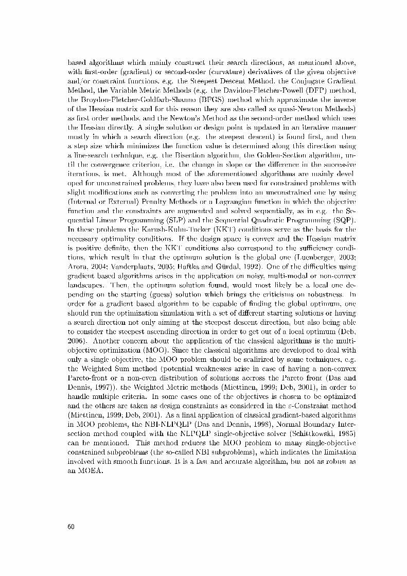
based algorithms which mainly construct their search directions, as mentioned above,with rst-order (gradient) or second-order (curvature) derivatives of the given objectiveand/or constraint functions, e.g. the Steepest Descent Method, the Conjugate GradientMethod, the Variable Metric Methods (e.g. the Davidon-Fletcher-Powell (DFP) method,the Broydon-Fletcher-Goldfarb-Shanno (BFGS) method which approximate the inverseof the Hessian matrix and for this reason they are also called as quasi-Newton Methods)as rst order methods, and the Newton's Method as the second-order method which usesthe Hessian directly. A single solution or design point is updated in an iterative mannermostly in which a search direction (e.g. the steepest descent) is found rst, and thena step size which minimizes the function value is determined along this direction usinga line-search technique, e.g. the Bisection algorithm, the Golden-Section algorithm, un-til the convergence criterion, i.e. the change in slope or the dierence in the successiveiterations, is met. Although most of the aforementioned algorithms are mainly devel-oped for unconstrained problems, they have also been used for constrained problems withslight modications such as converting the problem into an unconstrained one by using(Internal or External) Penalty Methods or a Lagrangian function in which the objectivefunction and the constraints are augmented and solved sequentially, as in e.g. the Se-quential Linear Programming (SLP) and the Sequential Quadratic Programming (SQP).In these problems the Karush-Kuhn-Tucker (KKT) conditions serve as the basis for thenecessary optimality conditions. If the design space is convex and the Hessian matrixis positive denite, then the KKT conditions also correspond to the suciency condi-tions, which result in that the optimum solution is the global one (Luenberger, 2003;Arora, 2004; Vanderplaats, 2005; Haftka and Gürdal, 1992). One of the diculties usinggradient based algorithms arises in the application on noisy, multi-modal or non-convexlandscapes. Then, the optimum solution found, would most likely be a local one de-pending on the starting (guess) solution which brings the criticisms on robustness. Inorder for a gradient based algorithm to be capable of nding the global optimum, oneshould run the optimization simulation with a set of dierent starting solutions or havinga search direction not only aiming at the steepest descent direction, but also being ableto consider the steepest ascending direction in order to get out of a local optimum (Deb,2006). Another concern about the application of the classical algorithms is the multi-objective optimization (MOO). Since the classical algorithms are developed to deal withonly a single objective, the MOO problem should be scalirized by some techniques, e.g.the Weighted Sum method (potential weaknesses arise in case of having a non-convexPareto-front or a non-even distribution of solutions accross the Pareto front (Das andDennis, 1997)), the Weighted Metric methods (Miettinen, 1999; Deb, 2001), in order tohandle multiple criteria. In some cases one of the objectives is chosen to be optimizedand the others are taken as design constraints as considered in the ε-Constraint method(Miettinen, 1999; Deb, 2001). As a nal application of classical gradient-based algorithmsin MOO problems, the NBI-NLPQLP (Das and Dennis, 1998), Normal Boundary Inter-section method coupled with the NLPQLP single-objective solver (Schittkowski, 1985)can be mentioned. This method reduces the MOO problem to many single-objectiveconstrained subproblems (the so-called NBI subproblems), which indicates the limitationinvolved with smooth functions. It is a fast and accurate algorithm, but not as robust asan MOEA.

60

3.1.2 Evolutionary Algorithms

Evolutionary algorithms (EAs) are non-deterministic (stochastic) methods that mimicevolutionary principles, e.g. natural selection and the survival of the ttest, to constitutetheir optimization strategy. They work with a set of solutions (population) instead of asingle point as in traditional (classical) methods and this gives an opportunity to attacka complex problem (discontinuous, noisy, multi-modal, etc.) in dierent directions allow-ing the algorithm to explore as well as exploit the search space. This capability gives anadvantage for having a more robust search strategy compared to traditional algorithms.Since they don't need any gradient information, they are very suitable for black-box (e.g.commercial software) optimization applications. Besides their relatively easy computa-tional implementation, they are also proper for distributed computing applications sinceall individuals (designs) can be computed independently. Due to their population basedsearch strategy, they have been more popular for the MOO problems, often having con-icting objectives resulting not only in a single optimum solution, but in a set of trade-osolutions (Pareto-optimal set), for the last last two decades. Many multi-objective evo-lutionary algorithms have been developed in order to solve multiple conicting goals inan ideal way, that is without using weightings between objectives or any scalarizationtechniques. Besides convergence, a well-spread distribution of these solutions across thePareto-front has been considered to be an important challenge for MOEAs. Some ofthe diculties that a MOEA may have to tackle have been pointed out by some re-searchers (Zitzler et al., 2000). TECHNICAL REPORT-I and TECHNICAL REPORT-II alsogive an overview of MOEAs and some of the well-known benchmark problems. The im-portance of the elitism concept, which allows the survival of the best solutions ever foundduring the generations, in MOO research was recognized and experimentally supportedby dierent studies (Parks and Miller, 1998; Zitzler et al., 2000). After some implemen-tations of non-elitist MOEAs (e.g. the Multi Objective Genetic Algorithm (MOGA) byFonseca and Fleming (1993), the Niched Pareto Genetic Algorithm (NPGA) by Hornet al. (1994) and the Non-dominated Sorting Genetic Algorithm (NSGA) by Srinivasand Deb (1994)), many new ones (e.g. the Strength Pareto Evolutionary Algorithm(SPEA and SPEA2) by Zitzler and Thiele (1998, 1999); Zitzler et al. (2001), the ParetoArchived Evolution Strategy (PAES) by Knowles and Corne (1998), the NSGA-II (thesuccessor of the NSGA) by Deb et al. (2002) and the Pareto Envelope-based SelectionAlgorithm (PESA) by Corne et al. (2000)) appeared incorporating elitism in dierentways. Evolutionary algorithms can be categorized into four major areas, i.e. Genetic Al-gorithms (GAs), Evolution Strategies (ESs), evolutionary programming (EP) and geneticprogramming (GP). Although their working principles are similar, there are still specicdierences that allow them to be specialized in some applications. More detailed infor-mation is given by Goldberg (1989); Deb (2001); Michalewicz (1992) and Mitchell (1998)on GAs, by Rechenberg (1973, 1997) and Schwefel (1995) on ESs, by Fogel (1999) on EP,by Koza (1993) and Poli et al. (2008) on GP, by De Jong (2006) on the general theory ofevolutionary computation and nally by Deb (2001); Miettinen (1999) and Branke et al.(2008) on the evolutionary and classical multiobjective optimization.

3.1.3 Hybrid Techniques

Although evolutionary computation has become an important problem solving methodol-ogy with its population-based collective learning process, self-adaptation, and robustness,the performance of the algorithms still depend on proper selection of various parameters

61

(e.g. probabilities, selection and mutation schemes, etc.), namely the proper relationshipbetween the exploration and the exploitation capabilities avoiding premature convergence,as mentioned above. Moreover, the computational speed is relatively slow as comparedto the classical (deterministic) algorithms. Therefore, as expected, the need for hybridalgorithms, which combine an evolutionary algorithm with e.g. a local search method,emerges, aiming at both robust and accurate solutions with (if at all possible) less compu-tational cost. Local search methods may be incorporated within the population members(parents) or among the osprings. The architectures of hybrid evolutionary algorithmshave been summarized by Grosan and Abraham (2007) as follows: hybridization betweentwo dierent EAs (a GP asisted GA), an EA with a neural network, a particle swarmoptimization (PSO) or an ant colony optimization (ACO) as well as hybridization be-tween EA and other heuristics (such as local search, tabu search, simulated annealing,hill climbing, etc.). However, as the No Free Lunch Theorem proposes, on average, allblack-box algorithms have identical behavior, thus there is not a denite answer for whichlocal search procedure to use for any sort of problems. Deb and Goel (2001) presentedsome test cases on shape optimization of mechanical components, i.e. a simply-supportedplate design, a cantilever plate design, a hoister design and a bicycle frame design, usingthe NSGA-II together with a hill-climbing local search method in order to move closerto the true Pareto-optimal front. In this approach, the results obtained from the MOEA(the NSGA-II) have been clustered for reducing the size of the non-dominated solutionset. Following this, the local search method is applied on each member of the reduced setby using a pseudo-weight vector for each solution to be used for the weighted objectivemetric which scalarizes the multiple conicting objectives, i.e. minimization of the weightand the deection of the structure. In another work by Ishibuchi and Murata (1998), adierent approach has been followed. The local search method is used during a GA runand applied on each solution before including it in the population, which is reportedto have less computational cost as compared to the posteriori approach that Deb andGoel (2001) used. Olympio (2007) hybridized the ε-NSGA-II, which uses ε-dominancefor population archiving and dynamic population sizing, by Kollat and Reed (2005) andthe weighting sum method for the local search as done by Deb and Goel (2001). First,this hybrid method (the HMOGA) was applied to three test problems (ZDT1, DTLZ3and DTLZ6), and then to a multi-objective topology optimization problem (related to thedesign of exible skins for a morphing aircraft) aiming at minimization of the tip deec-tion and the mass of the beam. The performance of the algorithm on the three test caseswas found to be better compared to the single MOGA case (without local search), butthe results for the topology optimization problem have been reported to be not satisfac-tory due to unrealistic solutions, i.e. related to chekerboard eects (mesh independencyltering was needed). Rigoni (2004a) applied another hybridization technique on somebenchmark cases, i.e. TNK, POL (these are also used in the TECHNICAL REPORT-I andII) and hole problems (Rigoni, 2004b), combining the NBI-NLPQLP with the MOGA-II.This methodology consists of starting with the MOGA-II computation then each singleportion of the Pareto-front (since it is discontinuous) is isolated as an independent prob-lem which is handled by an independent NBI-NLPQLP. Recently, Muller et al. (2009)succesfully combined the Evolution Strategy with Covariance Matrix Adaptation (CMA-ES) with the Particle Swarm Optimization (PSO) in order to solve highly noisy andmulti-funnel (valley) single objective optimization (SOO) problems where there are manylocal minima.

62

3.2 Description of the Algorithms

In the next two subsections, two algorithms, i.e. the Sequential Quadratic Programming(SQP) and the Non-dominated Sorting Genetic Algorithm (NSGA-II), will be describedin detail. The rst one is used in PAPER-I (Tutum et al., 2007) for the single-objectiveoptimization problem, whereas the second one is used in PAPER-III (Tutum et al., 2009),TECHNICAL REPORT-I and II for the multi-objective optimization cases.

3.2.1 Sequential Quadratic Programming (SQP)

The Sequential Quadratic Programming (SQP) method, which is a gradient-based opti-mization technique, represents the state of the art among nonlinear programming (NLP)methods. Schittkowski (1985) has implemented and tested a version that outperformsevery other tested methods in terms of eciency, accuracy and percentage of successfulsolutions over a large number of test problems. Due to its success, it was also implementedin both commercial softwares (e.g. NAG-SQP by NAG Ltd. (1988), DOT-SQP by Van-derplaats (1994), fmincon by The MathWorks Inc. (2006), part of Active Set Algorithmsin KNITRO by Waltz and Plantenga (2009), NLPQLP/MIPSQP/NBI-NLPQLP in mod-eFRONTIER by ESTECO s.r.l. (2007)) and open source environments (e.g. OpenOpt(2006), DONLP2 by Spellucci (1999)).

Based on the work of Powell (1978), the method is able to closely mimic the Newton'smethod (which is a second-order derivative method) for constrained optimization simi-lar to an unconstrained optimization. At each major iteration, an approximation of theHessian of the Lagrangian function is made using a quasi-Newton updating method, i.e.the BFGS (as Powell (1978) suggests) or the DFP, as mentioned in Section 3.1.1. This isthen used to generate a Quadratic Problem (QP) sub-problem, composed of a quadraticobjective function and linear constraints, whose solution is used to form a search directionfor a line search procedure (Luenberger, 2003; Arora, 2004; Vanderplaats, 2005). Despitethe high complexity of the QP-direction seeking algorithm, it is rewarded by faster con-vergence (Haftka and Gürdal, 1992). This method is also known as Iterative QuadraticProgramming, Recursive Quadratic Programming, or Constrained Variable Metric meth-ods.

For a given nonlinear constrained problem, as shown in Eq. (3.1),

Minimize : f(X)subject to : gj(X) ≤ 0, j = 1,m

hk(X) = 0, k = 1, l(3.1)

where f(X) is the objective function, X is the design point (vector) while gj(X)and hk(X) represent the inequality and the equality constraints, respectively, the QP-subproblem, which will provide a search direction S, is formulated as follows,

Minimize : q(S) = f(X) +∇f(X)TS+12STB(X, λ)S

subject to : ∇gj(X)TS+ gj(X) ≤ 0, j = 1,m

∇hk(X)TS+ hk(X) = 0, k = 1, l

(3.2)

63

where B is a positive denite approximation to the Hessian of the Lagrangian functionwhich is given below and λ is the vector of the Lagrange multipliers associated with theconstraints. The Lagrange multipliers in general are not only useful for checking optimal-ity (i.e. KKT conditions, as discussed in Section 3.1.1), but they also provide informationabout the sensitivity of the optimal solution to problem parameters, which can furtherbe interpreted as a measure of the eect of a change in the constraints on the objectivefunction (Haftka and Gürdal, 1992).

After the search direction (S) is found from the QP-subproblem, the design point willbe updated by,

Xi+1 = Xi + αS (3.3)

where the superscript-i denotes the iteration number, α is the unknown (scalar) stepsize to be moved along the search direction (S), which will be found by minimizing theLagrangian function (L),

L(X, λ) = f(X) +m∑

j=1

λjgj(X) +l∑

k=1

λm+k|hk(X)| (3.4)

The matrix B is initialized to some positive denite matrix (e.g. the identity matrix,I as represented in the owchart in Fig. 3.1) and then updated (B*) using the BFGSalgorithm,

B∗ = B− BppTB

pTBp+ηηT

pT η(3.5)

where,

p = Xi+1 −Xi (3.6)

η = θy+ (1− θ)Bp (3.7)

y = ∇xL(Xi+1, λi+1)−∇xL(Xi, λi) (3.8)

Here ∇x denotes the gradient of the Lagrangian (L) with respect to the design vector,X. In order to guarantee the positive deniteness of B, η is updated as shown above andθ is determined by Eq. (3.9).

θ =

1.0 if pTy ≥ 0.2pTBp

0.8pTBppTBp−pTy if pTy < 0.2pTBp

(3.9)

The owchart of the SQP algorithm is shown in Fig. 3.1.

64

Figure 3.1: The owchart of the SQP algorithm (Vanderplaats, 2005).

3.2.2 Non-dominated Sorting Genetic Algorithm (NSGA-II)

NSGA-II is a multi-objective evolutionary algorithm (MOEA) proposed by Deb et al.(2000a,b, 2002), which enables nding well-spread multiple Pareto-optimal solutions foran MOO problem by incorporating three substantial features, i.e. non-dominated sort-ing, an explicit diversity preserving mechanism and elitism. As the name indicates, it isthe next generation of its predecessor, i.e. the non-dominated sorting genetic algorithm(NSGA) (Srinivas and Deb, 1994), having substantial improvements with respect to com-putational complexity and robustness in the sense of having no need to use a sharingparameter (Goldberg and Richardson, 1987) to enforce diversity between the members.

In the case of SOOP (excluding multi-modal problems), it is easier to identify theoptimal solution compared to the case of MOOP where there are more than one criterionto satisfy, i.e. hence more than one best (elite) solution to consider. As it was put forwardby Goldberg (1989), "if we refuse to compare apples to oranges, then we must come upwith a dierent denition of optimality, one that respects the integrity of each of ourseperate criteria" which points out the concept of Pareto Optimality, correlated to thefundamental concept of domination.

Since the concept of domination allows a way to compare solutions with multiple ob-jectives, most MOO algorithms use this domination concept to search for non-dominatedsolutions, i.e. the ones that constitute the Pareto-front which will be described in Eq.(3.10). This concept can be explained with a simple example in 2D objective space, inwhich the minimization of both objective functions (i.e. f1 and f2) is considered, asshown in Fig. 3.2. In this gure, point-1 representing a solution or a design, e.g. an indi-vidual or a member in evolutionary computation parlance, splits the 2D objective spaceinto two zones: the rst zone (the shaded region); the set of the points dominated bypoint-1, and the second zone; the set of points not dominated by point-1 (the remainingthree quadrants), i.e. the non-dominated or noninferior set of points. Thus, the two

65

conditions stated below need to be satised if point-1 dominates point-i, where point-i isany other design point in the objective space (Deb, 2001):

point-1 is no worse than point-i in all objectives.

point-1 is strictly better than point-i in at least one objective.

These two statements give a general description for the comparison of the two solutionsin terms of "betterness", hence emphasizing the applicability of this comparison for othertypes or combinations of conicting objectives besides the minimization - minimizationtype as shown in Fig. 3.2, i.e. maximization - maximization, maximization - minimizationas well as minimization - maximization. In case of the aforementioned minimization-minimization problem, it is formulated as follows (Goldberg, 1989; Zitzler et al., 2000):

(∀j : fj(x1) ≤ fj (xi)) ∩ (∃k : fk(x1) < fk(xi)) (3.10)

where x1 represents point-1 in Fig. 3.2 and xi represents any design point-i in thesame 2D objective space. Eq. (3.10) can be put in words as; at least in one objective,design-1 is "less" than design-i, while in others they might be equal.

Figure 3.2: The two seperate sets of solutions dened with respect to point-1: i) the setof dominated solutions (the shaded region), ii) the set of non-dominated solutions.

The incremental scheme of an evolutionary algorithm will update the location of point-1 and bring it to a new location in 2D objective space, e.g. point-2, point-3, point-4 orpoint-5, as shown in Fig. 3.3. If point-1 is a solution from the previous generation andthe current generation contains point-4, then the new position is very a favorable one,since point-4 is not only non-dominated by point-1, but also point-4 dominates point-1. This kind of evolution is always desirable since it promotes convergence, thus thistransition has certainly to be preserved. On the other hand, if the evolutions bring point-1 to point-3 or point-5, the new point is also a non-dominated one, even though it isnot dominating point-1, eventually this transition should also be preserved in order toprovide a well-spread distribution of the points along the Pareto frontier.

66

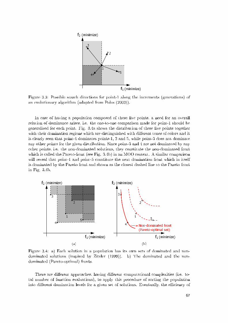
Figure 3.3: Possible search directions for point-1 along the increments (generations) ofan evolutionary algorithm (adapted from Poles (2003)).

In case of having a population composed of these ve points, a need for an overallrelation of dominance arises, i.e. the one-to-one comparison made for point-1 should begeneralized for each point. Fig. 3.4a shows the distribution of these ve points togetherwith their domination regions which are distinguished with dierent tones of colors and itis clearly seen that point-4 dominates points-1, 2 and 5, while point-3 does not dominateany other points for the given distribution. Since point-3 and 4 are not dominated by anyother points, i.e. the non-dominated solutions, they constitute the non-dominated frontwhich is called the Pareto-front (see Fig. 3.4b) in an MOO context. A similar comparisonwill reveal that point-1 and point-5 constitute the next domination front which in itselfis dominated by the Pareto front and shown as the closest dashed line to the Pareto frontin Fig. 3.4b.

(a) (b)

Figure 3.4: a) Each solution in a population has its own sets of dominated and non-dominated solutions (inspired by Zitzler (1999)). b) The dominated and the non-dominated (Pareto-optimal) fronts.

There are dierent approaches, having dierent computational complexities (i.e. to-tal number of function evaluations), to apply this procedure of sorting the populationinto dierent domination levels for a given set of solutions. Eventually, the eciency of

67

the sorting procedure is a critical issue in the case of a relatively high population size(e.g. N=100) and a high total number of generations (e.g. genmax=100) for real worldapplications, particularly depending on the computational cost of each design. Furtherdetails regarding the dierent sorting approaches are given in Deb (2001). The NSGA-IIuses a non-dominated sorting algorithm requiring O(MN2) overall computational com-plexity, where M is the number of objectives and N is the population size. It startswith calculation of the two entities for each member: a-) ni, the domination counter,which is the number of solutions which dominate the member-i, b) Si, which is a set ofmembers which the member-i dominates. It results in all the solutions across the rstnon-dominated front having a domination counter as zero (ni=0). Following the iden-tication of these non-dominated solutions, each member in their Si sets is visited andits domination counter is reduced by one. This procedure is repeated until all solutionsin the population are visited and their ni and Si entities are updated. In Fig. 3.5, vesolutions previously shown in Fig. 3.4 are presented with their nal domination informa-tion, i.e. solutions-3 and 4 having a domination counter of 1, solutions-1 and 5 having adomination counter of 2, and nally solution-2 having a domination counter of 3 as beingon the third and the last front.

Figure 3.5: Non-dominated sorting in the NSGA-II algorithm.

The preservation of well-distributed (diverse) nondominated solutions is maintainedby the crowding distance operator. The crowding distance, which is calculated frontwise,is a measure of how close an individual is to its neighbors. In order to get an estimate ofthe density of solutions surrounding a particular solution in the population, the averagedistance between two points on either side of the solution along each of the objectives iscalculated. This quantity di serves as an estimate of the perimeter of the cuboid formedby using the nearest neighbors as the vertices. A schematic view of the procedure forthe computation of the crowding distance for an ith individual is shown in Fig. 3.6, andformulated as (Deb et al., 2002),

dImi = dImi +f

(Imi+1)m − f (Imi−1)

m

fmaxm − fminm

, for i = 2, ..., l − 1 (3.11)

where I(i) is the solution index of the ith member in the (worse order) sorted list, mis the number of objectives and l is the number of the individuals in that particular front.

68

The rst and the last individuals are assigned an innite distance in order to emphasizetheir tness, hence preserving them for the next generation. A large average crowdingdistance will result in a better diversity in the population (Deb et al., 2002).

Figure 3.6: The crowding distance calculation (Deb et al., 2002).

After each member is sorted with respect to its own non-domination level (rank), thusis assigned a ttness equal to its rank as well as equiped with the crowding distance infor-mation, the next step is to select the good solutions, i.e. to emphasize the non-dominatedmembers, for the next generation. The binary tournament selection with a crowdedtournament operator is applied for this purpose. Shortly, the crowded tournament se-lection operator compares two solutions, i.e. with respect to their rank and crowdingdistance, and returns the winner of the tournament (comparison). The solution with thelower rank wins the tournament, but in case of having equal ranks, the solution with ahigher crowding distance, i.e. the member placed in a less crowded region, resolves thetie. The working principle of this operator can be shown in a simple case based on thedistribution of solutions as presented in Fig. 3.7. There are ten solutions in total and theyare sorted with respect to the non-domination criterion for the min.-min. problem, as aresult there are three fronts, i.e. the rst front is presented by the solutions with circlemarker, the second front with square marker and the third one is with diamond marker.These solutions constitute the set of parents. Children (ospring) are determined fromthis set by the binary tournament selection, meaning that, in particular for this case,ve pairs will be chosen twice and each solution (parent) will participate in exactly twotournaments. A random set of pairs is assummed as follows: (3,8), (10,9), (1,5), (2,4),(6,7), (3,10), (1,2), (4,6), (5,7), (8,9). In the rst tournament, solution 3 belongs to therst front and solution 8 belongs to the second front, thus solution 3 wins the tournamentsince it has a lower rank (it belongs to a better front). In the next tournament, bothsolutions 10 and 9 belong to the rst front (i.e. they have the same rank), hence in oderto resolve this tie, their crowding distance values will be checked. Since solution 9 is thelast member of the same front, i.e. the crowding distance is innite, and solution 10 has acrowding distance of a nite value, solution 9 is the winner of this tournament. Performingother tournaments will result in the following mating pool: 3, 9, 5, 4, 7, 3, 1, 4, 7, 9,which shows that solutions 3, 4, 7 and 9 are selected twice, meaning that members withlower rank are emphasized by the selection operator promoting convergence towards thePareto-front.

69

Figure 3.7: Ten solutions, i.e. non-dominated members presented with circles, the secondfront with squares and the third front with diamond, involved in the crowded tournamentselection.

In classical genetic algorithms (Goldberg, 1989), the internal encoding is based onbinary coding that each design variable is represented as a binary string, i.e. 0100,1101101, etc., where the length of the string depends on the number of allowed valuesfor the variable. The classical (single-point) cross-over is a well-known genetic algorithmoperator in which two parents (individuals from the mating pool) are randomly chosenand some portions of these binary strings are exchanged between each other. In single-point cross-over, the crossing site is randomly chosen and all bits on the right side of thecrossing site are swapped as shown "schematically" in Fig. 3.8.

Figure 3.8: Schematic procedure of single-point crossover.

This procedure is also shown for the same example given above (Fig. 3.8) in the2D parameter space in Fig. 3.9, assuming a representation of each variable with 5 bits(i.e. total string length of 10) considering an interval of [0,31] (the change in each bitcorresponds to an increment of 1).

The mutation operator is responsible for perturbing the binary string, i.e. changing1 to 0 or vice versa, with a given DNA String Mutation Ratio (probability). The mu-tation operator can be said to be responsible of the local search as well as maintainingthe diversity in the population (Deb, 2006).

However, some potential diculties arise in case of using binary coded GAs in thecontinuous parameter space, such as Hamming clis as well as the demand for a higherstring length depending on the prefered or required accuracy (which is unknown before-hand for the latter case). Hamming clis are observed while evolving from one solution

70

Figure 3.9: Representation of single-point crossover in 2D parameter space.

Figure 3.10: Schematic procedure of mutation for a given DNA string mutation ratio,pm=30%.

(e.g. encoded as string 0111111) to a neighboring solution (e.g. string 1000000) in realspace, which requires change of many bits (the longer the string, the more articial hin-drance is experienced) (Deb, 2001). The increase in the required precision (larger stringlength) calls for a larger population size (Goldberg et al., 1992) which in turn resultsin higher computational complexity. For these reasons, real-coded GAs (which do notrequire any encoding) are implemented in order to satify the need for better performancedemands on cross-over and mutation operators in the continuous search space. In theNSGA-II, simulated binary cross-over (SBX) (Deb and Agrawal, 1995; Deb and Kumar,1995) and polynomial mutation is used. The SBX operator uses two parent solutions asinputs and produces two children as output. As the name indicates, the SBX operatorsimulates the working principle of the single-point cross-over operator on binary strings.The original work is recommended for further details (Deb and Agrawal, 1995; Deb, 2001).

Figure 3.11: Schematic view of the NSGA-II procedure (Deb et al., 2002).

71

The schematic procedure of the NSGA-II is shown in 3.11. The procedure startswith an initialization of the parent population, P0, followed by sorting the members ofthe population based on nondomination into each front, Fi. Each individual is assignedtwo tness values, i.e. the one related to its nondomination level (front or rank, i.e. Firefers to front with rank i in Fig. 3.6) and the crowding distance. Parents are selectedby using the binary tournament selection (with crowded tournament operator) basedon these two measures. An individual is selected if its rank is less than the other is,since the minimization is assumed, or if its crowding distance is greater than the otheris. The selected population generates o-springs, Qt, by the application of usual geneticoperators, i.e. crossover, mutation, etc. (Goldberg, 1989). Since all the parent and theospring individuals are included in the combined population, Rt, elitism is ensured.In order to reduce the size of the population of the next generation from 2N to N ,nondomination sorting is applied and the individuals with the relatively lowest possibleranks are accomodated until the size of the population exceeds N . Then the individualsin front Fi are selected based on their crowding distance. This cycle is repeated until thestopping criterion, i.e. the total number of generations, is met. Further details can befound in the original study (Deb et al., 2002).

3.3 Optimization of the thermal models of FSW

3.3.1 Optimization of the analytical thermal model

The optimization case presented here was the rst one considered in the Ph.D. project,see PAPER-I. The problem is stated as the goal of nding the FSW parameters, i.e. heatinput and longitudinal welding speed, which provide a desired average temperature undersome process limitations. The problem can be formulated as in Eq. (3.12),

Minimize : f1(x) = (Taverage − 500)2 = F 2,

subject to : 0 < Qtot ≤ 10000W,0 ≤ uweld < 100mm/s.

(3.12)

where the objective function(F 2)is the error between the analytically or numerically

computed value and the desired average temperature under the tool shoulder. It would beadvantageous to obtain an analytical expression for the sensitivity computation based onEq. (2.6); however a semi-analytical procedure is presented. The necessary Finite Dier-ence calculations were performed for the COMSOL thermal model. Standard MATLABOptimization toolbox routines are used for the two equivalent optimization problems.

The nite element method gives the user the possibility to dene complicated models,including complex geometries and heat source models, etc., while analytical models havesome limitations in some aspects of the engineering applications, e.g. FSW modeling.In order to extend the applicability of the analytical formulation, a novel procedure isintroduced. The power of the moving line-type heat source is controlled by evaluating thetemperatures in a circular region surrounding the heat source and this is used as a processcontrol parameter. The corresponding bound constrained problem is solved using a sub-space trust region method based on the reective Newton method (The MathWorks Inc.,2006).

72

3.3.1.1 Derivation of the Closed Form Solution

A moving heat source representing the tool shoulder is described by a circle in an innitelyextended plate, as mentioned before and shown in Fig. 3.12. In order to obtain a closedform solution for the average temperature under the tool shoulder, the temperature elddened in Eq. (2.6) should be integrated over the circular area in polar coordinates, asformulated in Eq. (3.13).

Taverage =

∫A T dA∫A dA

=

∫ Rshr=0

∫ 2πθ=0 T (r, θ)rdθ drAcircle

,

=Qtot

2π2kdR2sh

∫ Rsh

r=0

∫ 2π

θ=0

rK0(wr)ewr cos(θ)

dθ dr + T0

(3.13)

The integral in Eq. (3.13) cannot be evaluated analytically due to the singularityof the K0 function in the formulation of the line-type heat source. Thus, a numericalintegration scheme will be dened in the following section.

Figure 3.12: A moving heat source in an innite plate dened in polar coordinates [ref.PAPER-I] (Tutum et al., 2007).

3.3.1.2 Numerical Computation of the Average Temperature

In this section, the numerical integration scheme for evaluating the average temperatureunder the tool shoulder is formulated. The line-type heat source is positioned in thecenter of the circle, dened as (0,0) in Cartesian coordinates, in Fig. 3.13.

73

Figure 3.13: A moving heat source in an innite plate dened in Cartesian coordinates[ref. PAPER-I] (Tutum et al., 2007).

Eq. (3.14) denes the average temperature, similar to Eq. (3.13), in a two dimensional(indices) summation form. Since all cells are equal in size, the denominator of Eq. (3.14)is reduced to the number of cells. The temperature values evaluated in the grid points(centers of the cells) placed in the circular area are summed easily, as dened individuallyin Eq. (2.6).

Taverage =

∑nii=1

∑njj=1 Tij(xi, yj) dAij∑nii=1

∑njj=1 dAij

=

∑nii=1

∑njj=1 Tij

ncell(3.14)

The grid size obviously inuences the accuracy of the average temperature expressiondened in Eq. (3.14). Thus, to ensure independence of this, a convergence test is per-formed by using the same heat input value for changing grid density along the diameter ofthe circular region representing the tool shoulder. Fig. 3.14 shows that the convergenceis achieved for a low number of increments.

Figure 3.14: Convergence test plot of the average temperature expression for dierentgrid size [ref. PAPER-I] (Tutum et al., 2007).

74

3.3.1.3 Semi-Analytical Sensitivities

The possibility to use analytical sensitivities provides substantial benets regarding sav-ings in computational cost. It is found, cf. Section 3.3.1.1, that it is not possible to obtaina closed form solution for the average temperature criterion since integration of the K0

function causes diculties. In this section, it is shown that the semi-analytical methodcan be used to reduce computational cost as much as possible. The sensitivities of theobjective function with respect to the welding parameters, i.e. heat input and weldingspeed, are dened in Eqs. (3.15) and (3.16), respectively.

d(F 2)dQtot

= 2F(

C

πR2

∫ R

0

∫ 2π

0

rK0(wr)ewr cos(θ)

dθdr

)=

2F (F + T1)q

(3.15)

d(F 2)duweld

= 2F C2

∫ R

0

∫ 2π

0

[r2

ewr cos(θ)(K1(wr) +K0(wr) cos(θ))

]dθdr (3.16)

Here F 2 denotes the objective function, T1=480K, C = 12πkd and C2 = −C Qtot

a whichare used to simplify the expressions and K1 is the Modied Bessel Function of the secondkind and the rst order. The rst sensitivity of the objective function with respect to theheat input is relatively easy to compute as compared to the second, since all variablesin Eq. (3.15) are already evaluated while computing the objective value as given in Eq.(3.12), using the incremental procedure. The second sensitivity expression is formulatedin an analytical way, but again evaluated using the incremental procedure.

3.3.2 Optimization of the numerical (Eulerian) thermal model

In this section, a steady state Eulerian heat ow model implemented in COMSOL is usedto control the average temperature under the tool shoulder. In order to nd the optimumwelding parameters, i.e. the heat input and welding speed for the bounded constrainedproblem as dened in Eq. (3.12), the Sequential Quadratic Method (SQP) with the BFGSline search algorithm is used (Vanderplaats, 2005). Finite dierence calculations are per-formed in order to obtain the sensitivity information.

The objective function eld for the corresponding design variable eld is shown inFig. 3.15a. It is obvious that multiple solutions are found since the optimization problemhas only simple boundaries without any equality or inequality constraints. The resultingoptimum curve which is labeled as the contour line equal to 1 is lying close to the zeroplane, as can be seen in Fig. 3.15b.

75

(a) (b)

Figure 3.15: a) Objective function eld (Error2) vs. design variable eld, i.e. heatinput and welding speed [ref. PAPER-I] (Tutum et al., 2007). b) Contour plot of thecorresponding objective function eld [ref. PAPER-I] (Tutum et al., 2007).

In order to evaluate the results from a practical viewpoint, the design variables, i.e.the heat input and the welding speed, are considered seperately. Tables 3.1 and 3.2 showthe results regarding the specied optimum design variable for the other xed weldingparameter, respectively. Aluminum is used as the workpiece material which is a 3 mm-thick plate. Notice that the analytical heat input solutions are scalable for dierent platethicknesses due to the linearity in terms of the heat generation density as given in Eq.(2.6).

Notice that the higher the welding speed is, the higher the error due to the boundaryeect. The analytical heat ow model does not see the eects of the boundary conditionsbecause of the innitely large domain description, while it is not the case for the numericalmodel having a nite domain. However, it can be concluded that the deviations betweenthe analytical and the numerical models are reasonable expecially for the lower weldingspeeds, which is also considerable for the FSW process.

Table 3.1: Comparison of the optimum heat input results for given welding speed andrelative error in relation to the analytical heat input [ref. PAPER-I] (Tutum et al., 2007)

uweld (mm/s) Qtot,Analytical (W) Qtot,COMSOL (W) |∆Qtot|Qtot,Analytical

(%)

2 575 585 2

4 780 890 14

6 971 1153 18

8 1160 1404 21

10 1350 1653 22

76

Table 3.2: Comparison of the optimum welding speed results for given heat input andrelative error in relation to the analytical welding speed [ref. PAPER-I] (Tutum et al.,2007)

Qtot (W) uweld,Analytical (mm/s) uweld,COMSOL (mm/s) |∆uweld|uweld,Analytical

(%)

500 1.36 1.50 10

750 3.69 3.00 18

1000 6.32 4.80 24

1250 8.97 6.80 24

1500 11.56 8.80 24

This section presented the rst optimization case considered in the Ph.D. work. Spe-cial about this was its relative simplicity being an SOO problem with some analyticalinformation available, thus calling for the probability of using a classical gradient basedoptimization algorithm. However in the following, some more complex MOO cases basedon thermo-mechanical models of FSW, applying genetic algorithms will be presented.

3.4 Optimization of the thermo-mechanical models of FSW

3.4.1 Optimization of the residual stresses and production rate in FSW

In the following sections we present a study of two multi-objective optimization prob-lems in the FSW process. These consider the minimization of the residual stresses in theworkpiece together with the maximization of the production eciency (reducing weldingtime and wear), respectively. These two objectives are conicting and techniques to dealwith this issue are also considered. The optimization procedure, which includes processintegration of the ANSYS software and the optimization algorithm (NSGA-II), is handledby applying modeFRONTIER. The optimization cycle is initiated by creating an initialpopulation of 16 pre-chosen Design-of -Computational-Experiments (DOE), for the con-sidered process variables, i.e. the tool rotational speed (revolutions per minute), n, andthe traverse welding speed, uweld. The FSW thermal and mechanical simulations, whichare built by using APDL in ANSYS, are coupled in a sequential way by execution of para-metric input les in a batch mode. The design variables are updated by the optimizationalgorithm and are read by the thermal analysis. Then the peak temperature obtainedat the end of the welding session is saved in order to be used as a thermal constrainttogether with the transient temperature eld results to yield the thermal strains for themechanical analysis. This mechanical analysis gives as a result the maximum longitudinalstress value at the middle of the plate in the transverse direction, and this is used as anobjective to be minimized. This optimization cycle runs until the stopping criterion, i.e.the total number of generations, is reached. The ow chart of the optimization procedureis shown in Fig. 3.16.

77

Figure 3.16: Flow chart of the optimization problem [ref. PAPER-III] (Tutum et al.,2009).

Most engineering design activities require a solution of multi-disciplinary and MOOproblems which usually deal with conicting design objectives. As discussed in Section3.2.2, the consideration of multiple conicting objectives results in a number of alternativetrade-os, called Pareto-optimal solutions, of which none can be said to be better thanany other without any additional information about the problem under consideration.This concept can be formulated as follows

(∀i : fi (x) ≤ fi (y)) ∩ (∃j : fj (x) < fj (y)) (3.17)

78

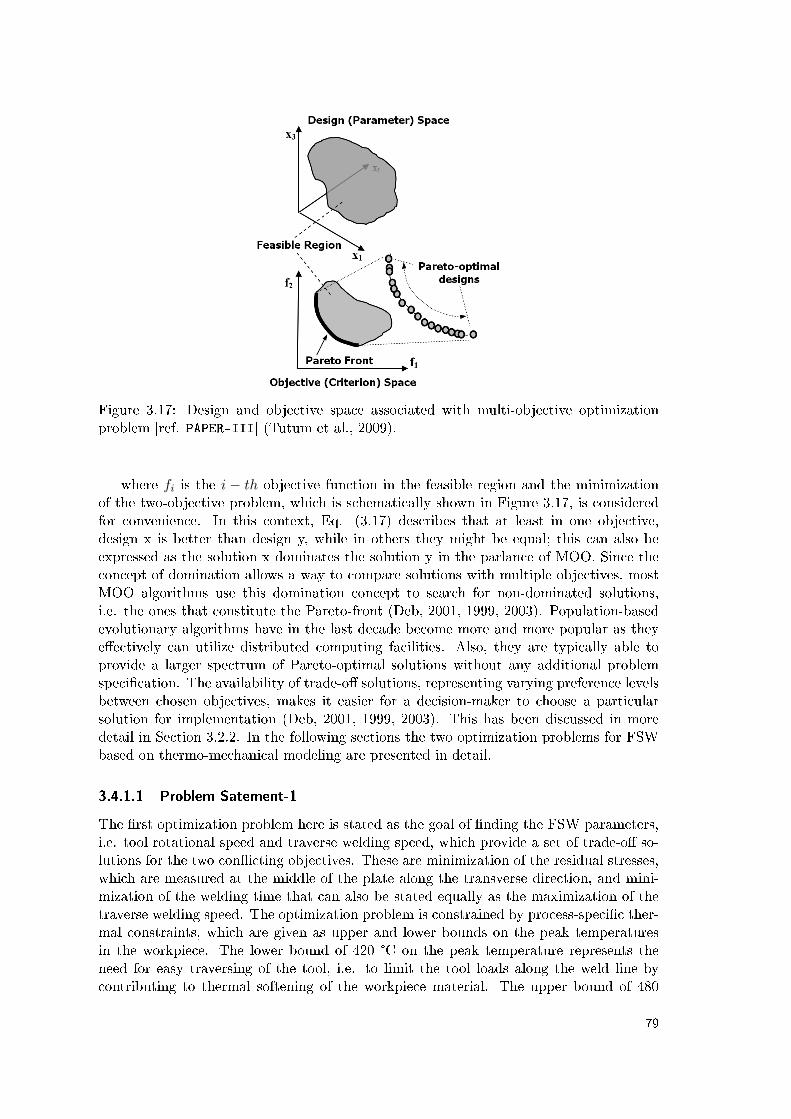
Figure 3.17: Design and objective space associated with multi-objective optimizationproblem [ref. PAPER-III] (Tutum et al., 2009).

where fi is the i − th objective function in the feasible region and the minimizationof the two-objective problem, which is schematically shown in Figure 3.17, is consideredfor convenience. In this context, Eq. (3.17) describes that at least in one objective,design x is better than design y, while in others they might be equal; this can also beexpressed as the solution x dominates the solution y in the parlance of MOO. Since theconcept of domination allows a way to compare solutions with multiple objectives, mostMOO algorithms use this domination concept to search for non-dominated solutions,i.e. the ones that constitute the Pareto-front (Deb, 2001, 1999, 2003). Population-basedevolutionary algorithms have in the last decade become more and more popular as theyeectively can utilize distributed computing facilities. Also, they are typically able toprovide a larger spectrum of Pareto-optimal solutions without any additional problemspecication. The availability of trade-o solutions, representing varying preference levelsbetween chosen objectives, makes it easier for a decision-maker to choose a particularsolution for implementation (Deb, 2001, 1999, 2003). This has been discussed in moredetail in Section 3.2.2. In the following sections the two optimization problems for FSWbased on thermo-mechanical modeling are presented in detail.

3.4.1.1 Problem Satement-1

The rst optimization problem here is stated as the goal of nding the FSW parameters,i.e. tool rotational speed and traverse welding speed, which provide a set of trade-o so-lutions for the two conicting objectives. These are minimization of the residual stresses,which are measured at the middle of the plate along the transverse direction, and mini-mization of the welding time that can also be stated equally as the maximization of thetraverse welding speed. The optimization problem is constrained by process-specic ther-mal constraints, which are given as upper and lower bounds on the peak temperaturesin the workpiece. The lower bound of 420 °C on the peak temperature represents theneed for easy traversing of the tool, i.e. to limit the tool loads along the weld line bycontributing to thermal softening of the workpiece material. The upper bound of 480

79

°C is dened in order to consider the tool life and the workpiece properties which areaected by hot welding conditions. This constrained multi-objective problem can thenbe expressed in mathematical terms as

Minimize : f1(x) = σx,max,

Maximize : f2(x) = uweld,

subject to : g1(x) = 420 oC ≤ Tpeak,g2(x) = Tpeak ≤ 480 oC,

where x =

uweld

n

,

uweld = 1, 2, ..., 10mm/s,n = 100, 200, ..., 1000 rpm.

(3.18)

where x represents the design variable vector, i.e. uweld, the traverse welding speedthat is changing from 1 mm/s to 10 mm/s in 1 mm/s increments and n, the tool rotationalspeed which varies from 100 rpm to 1000 rpm in 100 rpm increments (this results in 10discrete values in each design variable), σx,max denes the peak longitudinal stress, andTpeak is the peak temperature in the workpiece.

3.4.1.2 Results of Problem Satement-1

The solution of the rst optimization case, which is dened in section 3.4.1.1, is presentedin both the design and the criterion space in the following gures. Some of the designsout of a total of 320 designs (16 designs x 20 generations) are overlapping due to relativelycoarse discretization of the chosen design variables and also the selection operator. Thislies in the nature of the genetic algorithm that implies the survival of some designs withoutevolution. Fig. 3.18a and 3.18b represent feasible and unfeasible designs with dark andfair colors, respectively; constituting 49 dierent design points out of 100 (we use a 10x10discretization). The surface in each gure, i.e. the peak temperature and the peak residualstress, is constructed by 16 DOE points which are evaluated as an initial population forthe NSGA-II. It can be clearly seen from these gures that the feasible region, whichcan also be called the robust process parameter region in this case, is dened by n-valuesin the interval between 200 and 400 rpms. Due to the random evolution strategy ofEAs, some of the feasible solutions (4, 6, 8 mm/s with 200, 300 and 400 rpms), aremissing but the quality of these can be estimated from the surrounding solutions whichare positioned on a linearly varying region. Although the coarse discretization resultsin a few missing solutions, it is advantageous for having an overall idea regarding theoptimal feasible process frame with a moderate computational cost. In addition to this,the purpose of this study is to focus on the optimization methodology to nd and discussalternative trade-o solutions for minimization of welding residual stresses, i.e. not toconclude precise values. Having such solutions provides the engineer or manufacturerpractical insight about the relationship among process variables corresponding to thePareto-optimal solutions.

The objective space that is constructed by minimization of the residual stresses andmaximization of the welding speed is shown in Fig. 3.19a. Most of the designs lieclose to the Pareto-front, which is shown in Figure 10(b), due to the low sensitivity ofthe n parameter dened in the underlying thermal model, i.e. the TPM model for agiven welding speed on the residual stresses. If the minimum-residual stress solutions isconsidered to be of 100− 0% importance for product performance and process eciency,

80

(a) (b)

Figure 3.18: (a)Peak Temperature vs. design variables [ref. PAPER-III] (Tutum et al.,2009). (b)Residual stress vs. design variables [ref. PAPER-III] (Tutum et al., 2009).

respectively, then the maximum process eciency, i.e. welding speed or in other wordsthe production rate solution is of 0− 100% importance, thus the combination of 1 mm/sand 400 rpm would be chosen. If the other extreme solution, i.e. maximum weldingspeed, is considered, the combination of 10 mm/s and 400 rpm would be preferred. Incase of looking for the 70−30% trade-o solution for the same objectives, it is not clear toestimate the optimal combination of the process variables. Due to this desired preferencein objectives, the solution would be expected to be more similar to the minimum residualstress solution than the maximum production rate. It is important to note that thereare some dierent solutions satisfying such trade-o, but there is only one which is theoptimum, i.e. 4 mm/s and 400 rpm in this case. In other words, that solution makesthe optimum trade-o, meaning that for a particular amount of sacrice in one objective,the optimum solution will correspond to the maximum gain in the other objective (Deb,2003).

(a) (b)

Figure 3.19: (a)Objective Space of the solution [ref. PAPER-III] (Tutum et al., 2009).(b)Pareto Set of the solution [ref. PAPER-III] (Tutum et al., 2009).

All Pareto-optimal solutions correspond to the maximum feasible rotational speed

81

of 400 rpm while having dierent welding speeds varying from 1 mm/s to 10 mm/s.The Pareto-front shown in Fig. 3.19b gives an idea of ranking the alternative trade-osolutions depending on the available working conditions. If a manufacturer is able to usea standard milling machine instead of an advanced FSW machine and can aord usingsimple tool designs with low welding speed, he would probably not dare to go from 1 to 7mm/s in welding speed because the residual stresses yielded per unit increment in weldingspeed would cost higher comparing to those at higher welding speeds. The amount ofsacrice of the manufacturer relatively depends on the welding speed while one can keepthe rotation speed between 200 and 400 rpms.

3.4.1.3 Problem Satement-2

The second optimization problem, which is a slightly modied version of the rst case,Eq. (3.18), considers the minimization of the so-called wear path of an arbitrary pointon the tool shoulder besides taking the minimization of the residual stresses evolved onthe workpiece into account, simultaneously, Eq. (3.19).

Minimize : f1(x) = σx,max,

Minimize : f2(x) = ω/uweld,

subject to : g1(x) = 420 oC ≤ Tpeak,g2(x) = Tpeak ≤ 480 oC,

where x =

uweld

n

,

uweld = 1, 2, ..., 10mm/s,n = 100, 200, ..., 1000 rpm.

(3.19)

This wear path at the radius r at any point on the tool/workpiece interface can beapproximated by the following expression,

Lpath = vc tweld = ωrtweld = ωrLwelduweld

= (rLweld)ω

uweld= C

ω

uweld(3.20)

where subscript c denotes circumference and C is a parameter that will remain con-stant for the point under consideration. Minimization of the ratio of rotational speeddivided by welding speed corresponds to maximizing the tool advance per revolution.Other studies as explained below, have found weld property variations as a function ofeither welding speed divided by rotational speed, i.e. the weld pitch, rotational speeddivided by welding speed or pseudo heat index. However none of these are based on anargumentation addressing the wear criterion as presented in this paper, neither are theyused for optimization purposes, but more for process characterization and understanding.

It has been found out that, in general, the specic weld energy (Joules/meter) corre-lates with the weld pitch, i.e. the energy per unit length of weld increases as the weldpitch decreases (Seidel and Reynolds, 2001). The peak temperature in the weld zoneincreases with increasing the ratio of tool rotation rate/traverse speed (Hashimoto et al.,1999). The recrystallized grain size is reduced by decreasing the ratio of tool rotationrate/traverse speed which results in an increase in both degree of deformation and peaktemperature of the thermal cycle (Ma et al., 2002). The pseudo-heat index (ω2/uweld)was used as part of a generalized relationship in order to nd the peak temperature for

82

several aluminum alloys (Arbegast and Hartley, 1998). It was found that increasing theratio of rotational speed/traverse speed (ω/uweld) leads to a slight decrease in yield andultimate strength of the stir zone and transitional zone. It was also observed that increas-ing this ratio increases the weld nugget size and decreases the incomplete root penetration(Gharacheh et al., 2006).

3.4.1.4 Results of Problem Satement-2

The second optimization case dened in section 3.4.1.3 is presented below in objectivespace only since the design domain is kept constant while the solutions of the rst opti-mization case are rearranged by taking the tool rotational speed into account as shownin Fig. 3.20a and 3.20b.

From the Pareto front in Fig. 3.20b it is seen that at high welding speeds the secondobjective, i.e. minimization of the wear path becomes dominant, whereas for low weldingspeeds the rst objective of minimum residual stress is dominant.

It is also interesting to note that the wear path criterion divides the parameter spaceinto two intervals based on whether the welding speed is higher or lower than 5 mm/s.Thus, it is seen on Fig. 3.20b that for welding speeds above this value, the Pareto solutionsall have a rotational speed of 200 rpm, whereas for welding speeds below this value therotational speed varies between 200 and 400 rpm. So, as compared to the previouslyfound solutions, which are listed in section 3.4.1.4, the rotational speed is reduced from400 rpm to 200 rpm at high welding speeds resulting in a slightly higher sacrice in therst objective, i.e. minimization of the residual stresses.

(a) (b)

Figure 3.20: (a)Objective Space of the solution [ref. PAPER-III] (Tutum et al., 2009).(b)Pareto Set of the solution [ref. PAPER-III] (Tutum et al., 2009).

The discussions made for the rst problem case can be generalized for this case as well.The single optimum solution for the lowest welding speed is kept the same, i.e. beingcombined with a rotational speed of 400 rpm again, while the single optimum solutionfor the highest welding speed is rearranged in a way that it is combined with the lowestfeasible rotational speed, i.e. 200 rpm.

83

Chapter 4

Summary of Appended Papers

4.1 PAPER-I

C. C. Tutum, H. N. B. Schmidt, J. H. Hattel and M. P. Bendsøe, "Estimation of the

Welding Speed and Heat Input in Friction Stir Welding using Thermal Models and Opti-

mization", 7th World Congress on Structural and Multidisciplinary Optimization, COEX,Seoul, May 2007, Korea.

In this paper, the classical analytical solutions to the heat conduction equation in aEulerian frame as given by Rosenthal is programmed together with the correspondingnumerical thermal model in a Eulerian frame in the FE-software COMSOL Multiphysicsand good agreement is achieved as expected. This is then combined with an optimizationprocedure in which the objective is to achieve an average temperature of 500 °C underthe tool. The 500 °C is chosen as an indication of a suitable temperature level for thewelding process to succeed. The design variables for this optimization problem were thewelding speed and the heat input and the applied optimization algorithm was SequentialQuadratic Programming (SQP). Closed form expressions for the analytical sensitivitieswere derived.

4.2 PAPER-II

C. C. Tutum, H. N. B. Schmidt and J. H. Hattel, "Assessment of Benchmark Cases forModeling of Residual Stresses and Distortions in Friction Stir Welding", 7th InternationalSymposium on Friction Stir Welding, TWI, 2008, Awaji Island, Japan.

This paper presents a thermomechanical model for FSW, which is implemented inABAQUS and used to analyze several benchmark cases for the formation of residualstresses in FSW in which the eects of the clamping conditions and a temperature depen-dent yield stress are investigated. The ABAQUS model is also used for a more realisticcase in which the FSW of a stringer to a plate is modeled. The thermally induced residualstresses are calculated and subsequently the releasing and loading steps of the stringerstructure are modeled also. The results show that for the considered case, the loadingof the structure actually means a small reduction of the maximal longitudinal stresses ascompared to the residual stresses themselves.

85

4.3 PAPER-III

C. C. Tutum, H. N. B. Schmidt J. H. Hattel and M. P. Bendsøe, "A preliminary study on

optimization of residual stresses in friction stir welding", Materials and ManufacturingProcesses, 2009 (In press).

This paper presents a thermomechanical model for FSW, which is implemented inANSYS and used for a multiobjective optimization case in which the objectives are min-imizing the maximal residual stresses as well as maximizing the advancement per revo-lution which is given by the welding speed divided by the rotational speed. The designvariables are the welding speed and the rotational speed. This represents an example ofa multi-objective case in which the design variables are also part of one of the objectives.The results rst of all show that the NSGA-II algorithm works well together with thethermomechanical model in ANSYS and more specically they also reveal that increasingthe welding speed results in higher residual stresses for the case at hand. This mighthowever, not be the case for other constraining conditions.

4.4 PAPER-IV

J. H. Hattel, H. N. B. Schmidt and C. C. Tutum, "Thermomechanical Modelling of Fric-

tion Stir Welding", Proc. 8th International Conference on Trends in Welding Research,Pine Mountain, Atlanta, USA, 2008 (Invited keynote lecture).

In this paper, an overview of the thermomechanical modelling of the FSW process isgiven. The dierent types of models are classied based on the model discipline applied,i.e. numerical heat transfer models, computational solid mechanics models and com-putational uid dynamics models rather than from their purpose, i.e. thermal models,ow models and residual stress models. The formulation of all three mentioned mod-elling approaches are presented and discussed together with selected modelling resultsincluding prediction of material ow during welding, prediction of heat generation withthe thermal-pseudo mechanical model as well as residual stress and deformation analysiscombined with in-service loads.

4.5 TECHNICAL REPORT-I

C. C. Tutum and J. H. Hattel, "A benchmark study for unconstrained multi-objective

problems", September 2009.

In this report several well-known unconstrained Multi Objective Optimization (MOO)benchmark problems are investigated in order to analyze some of the diculties that aMulti Objective Evolutionary Algorithm (MOEA) may have to tackle. Three elitist algo-rithms, i.e. the MOGA-II, the NSGA-II and the cNSGA-II (custom NSGA-II implemen-tation by the author in MATLAB with two versions including an extra Pareto-optimalset achieved for post-processing purposes), are employed for this purpose.

86

4.6 TECHNICAL REPORT-II

C. C. Tutum and J. H. Hattel, "A benchmark study for constrained multi-objective prob-

lems", October 2009.

Similar to the TECHNICAL REPORT-I in its structure, however focusing on constrainedmulti-objective optimization benchmark problems. The results (especially for the con-strained case) show that the cNSGA-II shows a good performance for having both aconverged and a well-spread distribution of the Pareto-optimal set with a short compu-tational cost.

87

Chapter 5

Conclusions and Future Work

5.1 Conclusions

The work presented in this thesis focuses on two subjects; rst, the thermo-mechanicalmodeling of the FSW process, and secondly, the optimization of the thermal and thermo-mechanical aspects of the process by means of mathematical programming and evolution-ary computation techniques. The main conclusions and research achievements are brieysummarized below.

As a natural thing, the task of modeling the thermo-mechanical aspects of this com-plex process is initially divided into two steps, i.e. thermal and mechanical modeling.The thermal models are addressed rst since they in essence constitute the basis of allthe mechanical models, i.e. residual stress models, softening models or integrated modelswhich take the service load into account and damage evolution models.

In the rst optimization case, an optimal set of two process parameters, i.e. thewelding speed and the heat input, which aims for the process specic goal of obtainingan average temperature distribution under the tool is sought by using both analyticaland numerical Eulerian thermal models. These models are combined with a gradientbased optimization algorithm, i.e. Sequential Quadratic Programming (SQP) in order toinvestigate the optimal welding parameters as well as the applicability of these varying-complexity models. It is found that even a relatively simple analytical model can be usedto predict the temperature distribution ne enough under some assumptions and limits.Alongside with the optimization study, analytical sensitivities for the analytical modelare also obtained together with performing the similar nite dierence computations forsensitivities in the numerical model.

Following this, are the thermo-mechanical models implemented in both ABAQUSand ANSYS. Initially, these are used for the analysis of the transient temperature andstress evolutions during welding and subsequent cooling, eventually leading to the residualstress. It is well-known that some heat treated metals, e.g. aerospace aluminum alloysloose hardness and strength in the HAZ when subjected to thermal cycles during welding.This softening behavior was modeled and investigated for dierent (hot and cold) weldingconditions using ANSYS. The characteristics of the hardness proles for these conditionswere in good agreement with the experimental results published by other researchers.

89

Not common to literature, the subsequent loading situation of a real FSW structurewas also taken into account, thus making way for an integrated analysis of the weldingprocess and the loading situation during service of the welded part. This was also thetheme for another case, where the predicted stresses were combined with a subsequentuni-axial loading situation in which a damage evolution analysis was carried out in orderto predict the nal weld's load carrying capacity when subject to tension perpendicularto the weld line. It is found that taking the residual stresses into account increases themaximal stress a little, whereas the ductility of the specimen is reduced since the plasticow localization happens earlier during the loading process.

The thermo-mechanical models predicting residual stresses are subsequently combinedwith an evolutionary optimization algorithm (NSGA-II) in the search for the optimal com-bination of the process parameters that essentially are controllable in practice, namelythe welding speed and the rotational speed, which would minimize residual stresses andmaximize the welding speed divided by rotational speed (known as advancement per rev-olution and expressing a desired feature of the process). Being the rst result of its kindwhere optimization of FSW is based on residual stress analyses, the results rst of allshow that the NSGA-II algorithm (in modeFRONTIER) works well together with thethermo-mechanical model in ANSYS and more specically they also reveal that increas-ing the welding speed results in higher residual stresses for the case at hand. This mighthowever, not be the case for other constraining conditions.

This work is backed by some theoretical investigations regarding several well-knownunconstrained and constrained multi-objective optimization (MOO) benchmark prob-lems. This was done in order to investigate some of the diculties that a multi-objectiveevolutionary algorithm may have to tackle. Specically, the three elitist algorithms, i.e.the MOGA-II, the NSGA-II (the versions implemented in modeFRONTIER) and thecNSGA-II (custom NSGA-II implementation by the author in MATLAB) were employedfor this purpose. The results (especially for the constrained case) show that the cNSGA-IIshows a good performance for having both a converged and a well-spread distribution ofthe Pareto-optimal set in a short computational cost.

5.2 Future Work

The thermo-mechanical models (more specically the residual stress models) of the FSWprocess presented here have performed well for the proposed problems under practicallimitations. It would however be interesting to apply more detailed residual stress mod-els such as one combining both a local (for a detailed thermal analysis which takes thematerial ow into account) and a global (which aimes at capturing the overall behaviorof the welded structure, i.e. evolution of residual stresses and distortion) approach onthe same model. The more advanced residual stress models could involve more complexmaterial modelling approaches in which the yield stress is not only a function of the tem-perature, but also a function of the softening model which simulates the evolution of thematerial hardness.

Although the performance of the cNSGA-II algorithm is promising for the chosenbenchmark problems, it could be nice to test its performance on the numerical FSWmodels (e.g. residual stress models) where the exact Pareto-optimal front is not known.

90

Moreover, in order to improve the performance (the convergence towards the Pareto-optimal region) of the algorithm, a hybrid evolutionary approach which combines thecNSGA-II with a local search technique, e.g. a gradient-based optimization algorithm(SQP), could be very interesting. Besides FSW applications, a wide variety of manufac-turing processes, such as casting or glass moulding are other potential application areasfor the developed algorithm.

In order to make the number of function (design) evaluations as few as possible, espe-cially for these highly complex thermo-mechanical models of FSW, there is a substantialneed for the meta-modeling (approximation) techniques. These techniques are used tobuild relatively simple ("coarse"), thus computationally inexpensive models (surrogatemodels) instead of more-complicated, high-delity models, at the same time satisfying agood correspondance between these two. For example, response surface models (RSMs)or Design-of-Experiments (DOE) could be used to overcome those diculties related tocomputational resources. However, application of these methods could be challengingin multi-objective optimization problems as compared to single-objective optimizationproblems.

Besides those techniques mentioned above, distributed computing capabilities couldbe investigated. Due to their implicit or inherent parallelism, evolutionary algorithms arevery suitable for dierent types of parallel programming environments, such as massagepassing (MPI) or shared memory (e.g. OpenMP) applications. Due to its high scaling,distributed computing using MPI would be a natural choice. However, today, since multi-core architectures are being served almost as a standard with laptops, the shared memoryapplications (which allow the programmer update his/her original sequential-program toparallel-version without any substantial aords) are quite tempting as well.

91

Bibliography

Ansys Inc. (2007). http://www.ansys.com. (version 11.0).

Arbegast, W. and Hartley, P. (1998). Friction Stir Weld Technology Development atLockheed Martin MichoudSpace System - An Overview. USA. 5th International Con-ference on Trends in Welding Research.

Arora, J. (2004). Introduction to Optimum Design. Elsevier Inc.

Bellini, A., Hattel, J., and Thorborg, J. (2006). Thermo-mechanical modelling of alu-minium cast parts during solution treatment. Modelling and Simulation in Materials

Science and Engineering, 14:677688.

Belytschko, T., Liu, W., and Moran, B. (2000). Nonlinear Finite Elements for Continuaand Structures. John Wiley and Sons, Ltd.

Bendsøe, M. and Sigmund, O. (2003). Topology Optimization - Theory, Methods and

Application. Springer-Verlag.

Betounes, D. (1998). Partial dierential equations for computational science: with Maple

and vector analysis. Springer-Verlag New York, Inc.

Bhadeshia, H. (2003). Friction Stir Welding. http://www.msm.cam.ac.uk/

phase-trans/2003/FSW/aaa.html.

Bhide, B., Michaleris, P., Posoda, M., and DeLoach, J. (2006). Comparison of bucklingdistortion propensity for SAW, GMAW, and FSW. Welding Journal, pages 189195.

Bogomolny, M. and Bendsøe, M. (2007). Some Optimal Design Aspects of ResistanceWelding. pages 26872695. 7th World Congress on Structural and MultidisciplinaryOptimization.

Boley, B. and Weiner, J. (1960). Theory of Thermal Stresses. Dover Publications, Inc.

Branke, J., Deb, K., Miettinen, K., and Slowi«ski, R. (2008). Multiobjective Optimization

- Interactive and Evolutionary Approaches. Springer-Verlag.

Bussu, G. and Irving, P. (2003). The role of residual stress and heat aected zoneproperties on fatigue crack propagation in friction stir welded 2024-T351 aluminumjoints. International Journal of Fatigue, 25:7788.

Carslaw, H. and Jaeger, J. (1959). Conduction of heat in solids. Oxford University Press,USA.

93

Chao, Y. and Qi, X. (1998). Thermal and Thermo-Mechanical Modeling of Friction StirWelding of Aluminum Alloy 6061-T6. Computers and Structures, 7:215233.

Chu, C. and Needleman, A. (1980). Void nucleation eects in biaxially stretched sheets.Journal of Engineering Materials and Technology, 102:249256.

COMSOL AB (2007). http://www.comsol.com. (version 3.3a).

Cook, R., Malkus, D., Plesha, M., and Witt, R. (2001). Concepts and Applications of

Finite Element Analysis. John Wiley and Sons, Ltd.

Corne, D., Knowles, J., and Oates, M. (2000). The pareto envelope-based selectionalgorithm for multiobjective optimization. pages 839848. 6th International Conferenceon Parallel Problem Solving from Nature.

Criseld, M. (1991). Non-linear Finite Element Analysis of Solids and Structures - Vol-

ume 1: Essentials. John Wiley and Sons, Ltd.

Crumbach, M., Goerdeler, M., Gottstein, G., Neumann, L., Aretz, H., and Kopp, R.(2004). Through-process texture modelling of aluminium alloys. Modelling and Simu-

lation in Materials Science and Engineering, 12:S1S18.

Das, I. and Dennis, J. (1997). A closer look at drawbacks of minimizing weighted sums ofobjectives for Pareto set generation in multicriteria optimization problems. StructuralOptimization, 14:6369.

Das, I. and Dennis, J. (1998). Normal-Boundary Intersection: A new method for generat-ing the Pareto surface in nonlinear multicriteria optimization problems. SIAM Journal

on Optimization, 8:631657.

Dassault Systèmes (2007). http://www.simulia.com. (version 6.7-1).

De Jong, K. (2006). Evolutionary Computation: A Unied Approach. The MIT Press.

Deb, K. (1999). Multi-objective genetic algorithms: Problem diculties and constructionof test problems. Evolutionary Computation, 7:205230.

Deb, K. (2001). Multi-Objective Optimization using Evolutionary Algorithms. John Wileyand Sons, Ltd.

Deb, K. (2003). Unveiling innovative design principles by means of multiple conictingobjectives. Engineering Optimization, 35:445470.

Deb, K. (2006). Optimization for Engineering Design: Algorithms and Examples.Prentice-Hall of India Pvt. Ltd.

Deb, K. and Agrawal, R. (1995). Simulated binary crossover for continuous search space.Complex Systems, 9:115148.

Deb, K., Agrawal, S., Pratap, A., and Meyarivan, T. (2000a). A fast and elitist multi-objective genetic algorithm: NSGA-II. Technical report, Indian Institute of Technol-ogy, Kanpur: Kanpur Genetic Algorithms Laboratory (KanGAL).

94

Deb, K., Agrawal, S., Pratap, A., and Meyarivan, T. (2000b). A fast elitist non-dominatedsorting genetic algorithm for multi-objective optimization: NSGA-II. pages 849858.Parallel Problem Solving from Nature VI (PPSN-VI).

Deb, K. and Goel, T. (2001). A hybrid multi-objective evolutionary approach to engi-neering shape design. pages 385399. Evolutionary Multi-Criterion Optimization. FirstInternational Conference, EMO 2001.

Deb, K. and Kumar, A. (1995). Real-coded genetic algorithms with simulated binarycrossover: Studies on multi-modal and multi-objective problems. Complex Systems,9:431454.

Deb, K., Pratap, A., Agarwal, S., and Meyarivan, T. (2002). A fast and elitist multiobjec-tive genetic algorithm: NSGA-II. IEEE Transactions on Evolutionary Computation,6:182197.

Delahaye, J.-P. (2006). The science behind Sudoku. Scientic American, pages 8087.

Domkin, K. (2005). Constitutive models based on dislocation density - Formulation and

implementation into nite element codes. PhD thesis, Luleå University of Technology.

Dong, P., Hong, J., and Rogers, P. (1998). Analysis of residual stresses in Al-Li repairwelds and mitigation techniques. Welding Journal, 77:439445.

ESTECO s.r.l. (2007). http://www.esteco.com. (version v4.0).

Feng, Z. (2005). Processes and mechanisms of welding residual stress and distortion.Woodhead Publishing, Ltd.

Fogel, L.-J. (1999). Intelligence Through Simulated Evolution: Forty Years of Evolution-

ary Programming. John Wiley and Sons, Inc.

Fonda, R. and Lambrakos, S. (2002). Analysis of friction stir welds using an inverseproblem approach. Science and Technology of Welding and Joining, 7:177181.

Fonseca, C. and Fleming, P. (1993). Genetic algorithms for multiobjective optimization:Formulation, discussion and generalization. 5th International Conference on GeneticAlgorithms, USA.

Fratini, L. and Corona, V. (2007). Friction stir welding lap joint resistance optimiza-tion through gradient techniques. Journal of Manufacturing Science and Engineering,129:985990.

Frigaard, O. and Grong Ø, M. O. (2001). A process model for friction stir welding ofage hardening aluminum alloys. Metallurgical and Materials Transactions - Series A,32:11891200.

Gandin, C. A., Bréchet, Y., Rappaz, M., Canova, G., Ashby, M., and Shercli, H. (2002).Modelling of solidication and heat treatment for the prediction of yield stress of castalloys. Acta Materialia, 50:901927.

Geem, Z. (2007). Harmony Search Algorithm for Solving Sudoku. Lecture Notes in

Articial Intelligence, 4692:371378.

95

Geem, Z., Kim, J., and Loganathan, G. (2001). ANewHeuristicOptimizationAlgorithm:Harmony Search. Simulation, 76:6068.

Gharacheh, M., Kokabi, A., Daneshi, G., Shalchi, B., and Sarra, R. (2006). The inuenceof the ratio of "rotational speed/traverse speed" (ω/v) on mechanical properties ofAZ31 friction stir welds. Journal of Machine Tools & Manufacture, 46:19831987.

Goldberg, D. (1989). Genetic Algorithms in Search, Optimization & Machine Learning.Addison Wesley Longman, Inc.

Goldberg, D., Deb, K., and Clark, J. (1992). Genetic algorithms, noise, and the sizing ofpopulations. Complex Systems, pages 333362.

Goldberg, D. and Richardson, J. (1987). Genetic algorithms with sharing for multimodalfunction optimization. pages 4149. First International Conference on Genetic Algo-rithms and Their Applications.

Gould, J. and Feng, Z. (1998). Heat ow model for friction stir welding of aluminumalloys. Journal of Materials Processing & Manufacturing Science, 7:185194.

Grosan, C. and Abraham, A. (2007). Hybrid Evolutionary Algorithms: Methodologies,Architectures, and Reviews. Studies in Computational Intelligence, 75:117.

Gurson, A. (1977). Continuum theory of ductile rupture by void nucleation and growth.I. Yield criteria and ow rules for porous ductile media. Transactions of the ASME,

Journal of Engineering Materials and Technology, 99:215.

Haftka, R. and Gürdal (1992). Elements of Structural Optimization. Kluwer AcademicPublishers.

Hashimoto, T., Jyogan, S., Nakata, K., Kim, Y., and Ushio, M. (1999). FSW jointsof high strength aluminum alloy. USA. 1st International Symposium on Friction StirWelding.

Hattel, J. (2008). Integrated modelling in materials and process technology. Materials

Science and Technology, 24:137148.

Hattel, J., Schmidt, H., and Tutum, C. (2008). Thermomechanical modelling of FrictionStir Welding. USA. 8th International Conference on Trends in Welding ResearchConference, ASM.

Herdy, M. (1991). Application of the evolutionsstrategie to discrete optimization prob-lems. Parallel Problem Solving from Nature. 1st Workshop, PPSN 1 Proceedings.

Hooke, R. and Jeeves, T. (1961). Direct search solution of numerical and statisticalproblems. Journal of the Association for Computing Machinery, 8:212229.

Horn, J., Nafpliotis, N., and Goldberg, D. (1994). A niched Pareto genetic algorithmfor multiobjective optimization. pages 8287. First IEEE Conference on EvolutionaryComputation. IEEE World Congress on Computational Intelligence.

Huiskes, R., Weinans, H., Grootenboer, H., Dalstra, M., Fudala, B., and Sloo, T. (1987).Adaptive bone-remodeling theory applied to prosthetic-design analysis. Journal of

Biomechanics, 20:11351150.

96

Ishibuchi, H. and Murata, T. (1998). A multi-objective genetic local search algorithm andits application to owshop scheduling. pages 392403. IEEE Transactions on Systems,Man and Cybernetics, Part C.

Jahazi, M., Dubourg, L., and Cao, X. (2008). Friction Stir Weldingof Aerospace Alloys. http://www.smecanada.ca/montreal/presentations/

Jahazi-Mohammad-FSW.pdf. (presentation).

James, M., Hughes, D., Chen, Z., Lombard, H., Hattingh, D., Asquith, D., Yates, J., andWebster, P. (2007). Residual stresses and fatigue performance. Engineering Failure

Analysis, 14:384395.

Kennedy, J. and Eberhart, R. (1995). Particle swarm optimization. pages 19421948.IEEE International Conference on Neural Networks Proceedings.

Kermanpur, A., Tin, S., Lee, P., and McLean, M. (2004). Integrated modeling for themanufacture of aerospace discs: grain structure evolution. Minerals, Metals & Mater.

Soc, USA, 56:7278.

Khan, A. and Huang, S. (1995). Continuum Theory of Plasticity. John Wiley and Sons,Ltd.

Knowles, J. and Corne, D. (1998). The pareto archived evolution strategy: A new baselinealgorithm for pareto multiobjective optimization. pages 250259. Parallel ProblemSolving from Nature - PPSN V. 5th International Conference.

Kollat, J. and Reed, P. (2005). Comparing state-of-the-art evolutionary multi-objectivealgorithms for long-term groundwater monitoring design. Advances in Water Resources,29:792807.

Koza, J. (1993). Genetic programming: on the programming of computers by means of

natural selection. The MIT Press.

Lakshminarayanan, A. and Balasubramanian, V. (2008). Process parameters optimizationfor friction stir welding of RDE-40 aluminum alloy using Taguchi technique. Trans.

Nonferrous Met. Soc. China, 18:548554.

Larsen, A., Bendsoe, M., Hattel, J., and Schmidt, H. (2009). Optimization of frictionstir welding using space mapping and manifold mapping an initial study of thermalaspects. Struct. Multidisc. Optim., 38:289299.

Lindgren, L. (2007). Computational Welding Mechanics: Thermomechanical and

Microstructural Simulations. Woodhead Publishing, Ltd.

Lombard, H., Hattingh, D., Steuwer, A., and James, M. (2008). Optimising FSW processparameters to minimise defects and maximise fatigue life in 5083-h321 aluminum alloy.Engineering Fracture Mechanics, 75:341354.

Lubliner, J. (1990). Plasticity Theory. Macmillan Publishing Company.

Luenberger, D. (2003). Linear and Nonlinear Programming. Kluwer Academic Publish-ers.

97

Lundbäck, A., Alberg, H., and Henrikson, P. (2005). Simulation and validation of TIG-welding and post weld heat treatment of an inconel 718 plate. Mathematical Modellingof Weld Phenomena 7, Technische Universität, Graz.

Ma, Z., Mishra, R., and Mahoney, M. (2002). Superplastic deformation behaviour offriction stir processed 7075Al alloy. Acta Materialia, 50:44194430.

Mantere, T. and Koljonen, J. (2008). Solving, rating and generating sudoku puzzles withGA. IEEE Congress on Evolutionary Computation, CEC 2007.

Marie, F. and Allehaux, D. (2006). Development of FSW for optimum run-out perfor-mance. 6th International Symposium on Friction Stir Welding, Canada.

Mattheck, C. (1997). Design in Nature: Learning from Trees. Springer-Verlag.

Mattheck, C. and Burkhardt, S. (1990). A new method of structural shape optimizationbased on biological growth. International Journal of Fatigue, 12:185190.

McClure, J., Tang, W., Murr, L., Guo, X., Feng, Z., and Gould, J. (1998). A thermalmodel of friction stir welding. USA. 5th International Conference on Trends in WeldingResearch.

Metropolis, N., Rosenbluth, A., Rosenbluth, M., Teller, A., and Teller, E. (1953). Equa-tion of state calculations by fast computing machines. Journal of Chemical Physics,21:10871092.

Michaleris, P., Dantzig, J. A., and Tortorelli, D. (1999). Minimization of welding residualstress and distortion in large structures. Welding Journal, 78:361s366s.

Michaleris, P. and Sun, X. (1997). Finite Element Analysis of Thermal TensioningTechniques Mitigating Weld Buckling Distortion. Welding Journal, 76:451s457s.

Michalewicz, Z. (1992). Genetic Algorithms+Data Structures=Evolution Programs.Springer-Verlag.

Miettinen, K. (1999). Nonlinear Multiobjective Optimization. Kluwer Academic Pub-lishers.

Mishra, R. and Ma, Z. (2005). Friction stir welding and processing. Materials Science

and Engineering R, 50:178.

Mishra, S. and DebRoy, T. (2007). Tailoring gas tungsten arc weld geometry using aGA and a NN trained with convective heat ow calculations. Materials Science and

Engineering A, 454-455:477486.

Mitchell, M. (1998). An Introduction to Genetic Algorithms. The MIT Press.

Muller, C., Baumgartner, B., and Sbalzarini, I. (2009). Particle Swarm CMA EvolutionStrategy for the optimization of multi-funnel landscapes. pages 26852692. IEEECongress on Evolutionary Computation (CEC 2009).

Murphy, A., McCune, W., Quinn, D., and Price, M. (2007). The characterization offriction stir welding process eects on stiened panel buckling performance. Thin-

Walled Structures, 45:339351.

98

Murr, L., Liu, G., and McClure, J. (1997). Dynamic recrystallisation in the friction-stirwelding of aluminium alloy 1100. Journal of Materials Science Letters, 16:18011803.

Myhr, O. and Grong, O. (1991a). Process Modelling Applied to 6082-T6 AluminumWeldments - 1. Reaction Kinetics. Acta metall. mater, 39:26932702.

Myhr, O. and Grong, O. (1991b). Process Modelling Applied to 6082-T6 AluminumWeldments - 2. Applications of model. Acta metall. mater, 39:27032708.

Myhr, O., Grong, O., Fjaer, H., and Marioara, C. (2004). Modelling of the microstructureand strength evolution in Al-Mg-Si alloys during multistage thermal processing. ActaMaterialia, 52:49975008.

NAG Ltd. (1988). The NAG Fortran library manual. Numerical Algorithms Group Ltd.,Oxford, UK.

Nandan, R., DebRoy, T., and Bhadeshia, H. (2008a). Recent advances in friction stirwelding - process, weldment structure and properties. Progress in Materials Science,53:9801023.

Nandan, R., Lienert, T., and DebRoy, T. (2008b). Toward reliable calculations of heat andplastic ow during friction stir welding of ti-6al-4v alloy. Int. J. Mat. Res., 99:434444.

Nelder, J. and Mead, R. (1965). A simplex method for function minimization. ComputerJournal, 7:308313.

Nielsen, K. (2008). Ductile damage development in friction stir welded aluminum(AA2024)joints. Engineering Fracture Mechanics, 75:27952811.

Nielsen, K. and Tvergaard, V. (2009). Eect of ashear modied Gurson model on damagedevelopment in a fsw tensile specimen. International Journal of Solids and Structures,46:587601.

Olympio, K. (2007). A Hybrid Multi-Objective Genetic Algorithm for TopologyOptimization. http://water.engr.psu.edu/reed/Education/CE\%20563\

%20Projects/ce563_olympio_project\%20\%20Sp\%2007.pdf.

OpenOpt (2006). http://openopt.org. Free Python-written numerical optimizationframework. Optimization Department of Cybernetics Institute, National Academy ofSciences of Ukraine.

Parks, G. and Miller, I. (1998). Selective breeding in a multiobjective genetic algorithm.pages 250259. Parallel Problem Solving from Nature - PPSN V. 5th InternationalConference.

Peel, M., Steuwer, A., Preuss, M., and Withers, P. (2003). Microstructure, mechanicalproperties and residual stresses as afunction of welding speed in aluminum AA5083friction stir welds. Acta Materialia, 51:47914801.

Poles, S. (2003). MOGA-II: An improvedMulti-Objective Genetic Algorithm. Technicalreport, ESTECO s.r.l.

Poli, R., Langdon, W., and McPhee, N. (2008). A eld guide to genetic programming.http://www.gp-field-guide.org.uk.

99

Poloni, C. and Pediroda, V. (1997). GA coupled with computationally expensive simula-

tions: tools to improve eciency, chapter Genetic Algorithms and Evolution Strategiesin Engineering and Computer Science, pages 267288. John Wiley and Sons.

Powell, M. (1964). An ecient method for nding the minimum of a function of severalvariables without calculating derivatives. The Computer Journal, 7:155162.

Powell, M. (1978). A fast algorithm for nonlinearly constrained optimization calcula-tions. volume 630 of Lecture Notes in Mathematics, pages 144157. Springer Berlin -Heidelberg-New York.

Priesterjahn, S. (2007). Imitation-Based Evolution of Articial Game Players. SIGEVO-lution, newsletter of the ACM Special Interest Group on Genetic and EvolutionaryComputation. Volume 2, Issue 4, pp. 2-13.

Radaj, D. (1992). Heat Eects of Welding Temperature Field, Residual Stress and Dis-

tortion. Springer-Verlag Berlin Heidelberg.

Rechenberg, I. (1973). Evolutionsstrategie: Optimierung Technischer Systeme nach

Prinzipien der Biologischen Evolution. Frommann-Holzboog Verlag.

Rechenberg, I. (1997). Bionik & evolutionstechnik. http://www.bionik.tu-berlin.de.

Richards, D., Pragnell, P., Williams, S., and Withers, P. (2008a). Global mechanicaltensioning for the management of residual stresses in welds. Materials Science and

Engineering A, 489:351362.

Richards, D., Prangnell, P., Withers, P., Williams, S., Nagy, T., and Morgan, S. (2008b).Simulation of the eectiveness of dynamic cooling for controlling residual stresses infriction stir welds. 7th International Symposium Friction Stir Welding, TWI.

Rigoni, E. (2004a). Bench-marking NBI-NLPQLP. Technical Report 4, ESTECO s.r.l.

Rigoni, E. (2004b). Hole functions problem. Technical Report 2, ESTECO s.r.l.

Robin, V., Bernauer, G., Akgün, T., and Heubrandtner, T. (2005). Spotweld performanceunder high strain rate loading conditions. Mathematical Modelling of Weld Phenomena7, Technische Universität, Graz.

Rosenthal, D. (1946). The theory of moving sources of heat and its application to metaltreatments. Transactions of the American Society of Mechanical Engineers, 68:849865.

Russell, M. and Shercli, H. (1999). Analytical modelling of microstructure developmentin friction stir welding. USA. 1st International Symposium on Friction Stir Welding.

Satoh, K. (1972). Transient thermal stresses of weld heat-aected zone by-both-ends-xedbar analogy. Transactions of the Japan Welding Society, 3:125134.

Schittkowski, K. (1985). NLPQL: A fortran subroutine solving constrained nonlinearprogramming problems. Annals of Operations Research, 5:485500.

Schmidt, H. and Hattel, J. (2004). An analytical model for the heat generation in frictionstir welding. Modeling and Simulation in Materials Science and Engineering, 12:143157.

100

Schmidt, H. and Hattel, J. (2005). Modeling the heat ow around tool probe in frictionstir welding in friction stir welding. Science and Technology of Welding and Joining,10:176186.

Schmidt, H. and Hattel, J. (2008a). Thermal modeling of friction stir welding. Scripta

Materialia, 58:332337.

Schmidt, H. and Hattel, J. (2008b). A thermal-pseudo-mechanical model for the heatgeneration in Friction Stir Welding. Japan. 7th International Symposium on FrictionStir Welding.

Schwefel, H.-P. (1995). Evolution and Optimum Seeking. John Wiley and Sons, Inc.

Seidel, T. and Reynolds, A. (2001). Visualization of the material ow inAA2195 Friction-Stir Welds using a marker insert technique. Metallurgical and Materials Transactions

A, 32A:28792884.

Simo, J. and Hughes, T. (1998). Computational Inelasticity. Springer-Verlag New York,Inc.

Skillingberg, M. and Green, J. (2007). Aluminum applications in the rail industry. LightMetal Age.

Spellucci, P. (1999). DONLP2 Short Users Guide. Technische Universität Darmstadt,Darmstadt, Germany.

Srinivas, N. and Deb, K. (1994). Multi-objective optimization using non-dominated sort-ing in genetic algorithms. Evolutionary Computation, 2:221248.

Storn, R. and Price, K. (1997). Dierential Evolution - a simple and ecient heuristic forglobal optimization over continuous spaces. Journal of Global Optimization, 11:341359.

Tanev, I. and Shimohara, K. (2007). Towards human competitive driving of scale modelof a car. SIGEVOlution, newsletter of the ACM Special Interest Group on Genetic andEvolutionary Computation. Volume 2, Issue 4, pp. 14-26.

The MathWorks Inc. (2006). MATLAB Optimization Toolbox Users Guide.

The MathWorks Inc. (2007). http://www.mathworks.com. (release R2007b).

Thorborg, J., Hald, J., and Hattel, J. (2006). Stellite failure on a P91 HP valve - Failureinvestigation and modelling of residual stresses. Welding in the World, 50:4051.

Tutum, C. (2005). Structural optimization of truss structures subjected to stress, displace-ment, buckling and natural frequency constraints. Master's thesis, Istanbul TechnicalUniversity, Istanbul, TR.

Tutum, C. (2006). Structural optimization of truss structures subjected to stress, dis-placement, buckling and natural frequency constraints. FGES Users Conference.

Tutum, C. (2007a). Modelling of residual stresses in friction stir welding. Presentaion atthe INNOJOINT Meeting.

101

Tutum, C. (2007b). Computational Welding Mechanics. Danish Center of AppliedMechanics and Mathematics (DCAMM) Ph.D. Course Report.

Tutum, C. and Hattel, J. (2008). Notes on the modeling of welding process course(41741). Technical report, Technical University of Denmark, Department of MechanicalEngineering.

Tutum, C., Schmidt, H., and Hattel, J. (2008a). Assessment of benchmark cases for mod-eling of residual stresses and distortions in friction stir welding. Japan. 7th InternationalSymposium on Friction Stir Welding.

Tutum, C., Schmidt, H., and Hattel, J. (2008b). Optimization of the process parame-ters for controlling residual stress and distortion in friction stir welding. InternationalConference on Simulation Based Engineering and Sciences, TCN CAE.

Tutum, C., Schmidt, H., Hattel, J., and Bendsøe, M. (2007). Estimation of the weldingspeed and heat input in friction stir welding using thermal models and optimization.7th World Congress on Structural and Multidisciplinary Optimization, Seoul.

Tutum, C., Schmidt, H., Hattel, J., and Bendsøe, M. (2009). A preliminary study onoptimization of residual stresses in friction stir welding. (In press) "Journal of Materialsand Manufacturing Processes".

Tvergaard, V. (2001). Plasticity and creep in structural materials. Department of Me-chanical Engineering, Solid Mechanics, Technical University of Denmark.

Tvergaard, V. and Needleman, A. (1984). Analysis of the cup-cone fracture in a roundtensile bar. Acta Metallurgica, 32:157169.

TWI (1991). Friction stir welding at TWI. http://www.twi.co.uk/content/fswintro.html.

Vanderplaats, G. (1994). DoT User Manual. VMA Engineering, Colorado Springs, CO,USA.

Vanderplaats, G. (2005). Numerical Optimization Techniques for Engineering Design.Vanderplaats Research & Development, Inc.

Vecchi, M. and Kirkpatrick, S. (1983). Global wiring by simulated annealing. IEEE

Transactions on Computer-Aided Design of Integrated Circuits and Systems, 2:215222.

Vilaça, P., Quintino, L., and dos Santos, J. (2005). Analytical thermal model for frictionstir welding. Journal of Materials Processing Technology, 169:452465.

Waltz, R. and Plantenga, T. (2009). KNITRO 6.0 Users Manual. Ziena Optimization,Inc., Evanston, IL, USA.

Wikipedia (last modied on 1 November 2009b). Rubik's Cube. http://en.wikipedia.org/wiki/Rubik's_Cube.

Wikipedia (last modied on 24 July 2009a). Friction stir welding. http://en.wikipedia.org/wiki/Friction_stir_welding.html.

102

Wikiquote (last modied on 7 June 2008). George e. p. box. http://en.wikiquote.

org/wiki/George_E._P._Box.

Zhu, X. and Chao, Y. (2002). Eects of temperature-dependent material properties onwelding simulation. Computers and Structures, 80:967976.

Zitzler, E. (1999). Evolutionary Algorithms for Multiobjective Optimization: Methods and

Applications. PhD thesis, Swiss Federal Institute of Technology (ETH), Zurich.

Zitzler, E., Deb, K., and Thiele, L. (2000). Comparison of multiobjective evolutionaryalgorithms: Emprical results. Journal of Evolutionary Computation, 8:173195.

Zitzler, E., Laumanns, M., and Thiele, L. (2001). SPEA2: Improving the Strength ParetoEvolutionary Algorithm. Technical Report 103, Swiss Federal Institute of Technology(ETH) Zurich.

Zitzler, E. and Thiele, L. (1998). An evolutionary algorithm for multiobjective optimiza-tion: the Strength Pareto approach. Technical Report 43, Swiss Federal Institute ofTechnology (ETH) Zurich.

Zitzler, E. and Thiele, L. (1999). Multiobjective evolutionary algorithms: a comparativecase study and the Strength Pareto approach. IEEE Transactions on Evolutionary

Computation, 3:257271.

103

Appendixes

105

A PAPER-I

C. C. Tutum, H. N. B. Schmidt, J. H. Hattel and M. P. Bendsøe, "Estimation of the

Welding Speed and Heat Input in Friction Stir Welding using Thermal Models and Opti-

mization", 7th World Congress on Structural and Multidisciplinary Optimization, COEX,Seoul, May 2007, Korea.

107

Estimation of the Welding Speed and Heat Input in Friction Stir Welding using Thermal Models and Optimization

Cem C. Tutum1, Henrik Schmidt1, Jesper Hattel1, Martin P. Bendsøe2

1 Department of Manufacturing Engineering and Management, Technical University of Denmark, Lyngby,

Denmark, cem@ipl.dtu.dk 2 Department of Mathematics, Technical University of Denmark, Lyngby, Denmark

Abstract The objective of this work is to study the applicability of a relatively simple analytical thermal model for optimizing the welding parameters in Friction Stir Welding (FSW), i.e. heat input and welding speed, based on the assumptions of constant heat generation under the tool shoulder and symmetric heat flow along the welding line. A procedure to simulate the distributed heat source present in the real FSW process has been developed using a much simpler line source description. The range of applicability of the simplified model has also been investigated using more advanced numerical models. Sequential Quadratic Programming (SQP) is used for solving the optimization problem, in which the objective function is defined as the average temperature under the tool shoulder. Process related constraints are also included in the problem. Analytical and numerical sensitivity analyses are performed for the analytical and numerical models, respectively. Keywords: Friction Stir Welding; Constrained Optimization; Analytical Thermal Model; Eulerian Finite Element Model 1. Introduction

Friction Stir Welding (FSW) is an efficient solid-state joining technique that is invented especially for aluminum alloys [1]. Improved mechanical properties, reduced distortion and residual stresses, and environment friendliness are some of its advantages [2]. The requirement for lighter structures, especially in aerospace, automotive and railway industries, emphasizes the need for the FSW process to be better understood. The FSW process consists of several subsequent procedures here denoted as plunging, dwelling, actual welding and pulling the tool out of the work piece. First, the tool is submerged vertically into the joint line with high rotation speed, e.g. 400-1250 rpm, in the plunge period and then the dwell period takes place, where the tool is held steady relative to the work piece while rotating. Heat dissipation due to the friction and material deformation causes material to soften and allows traversing of the tool along the joint line. After initiation of the actual welding period, combination of sliding and sticking conditions under the tool shoulder plays an important role in obtaining preferred temperature ranges [3]. Following the welding period, the tool is pulled out of the work piece leaving a key hole behind. New analytical and numerical models are being studied by many research groups in order to improve the process efficiency and performance of the components. Various aspects of modeling FSW are possible regarding microstructure evolution, material and heat flow, heat generation, investigation of the influence of process parameters, residual stress computation, predicting mechanical loads (tool forces, torque and adjustment of work piece fixture, etc.) and final mechanical properties of the joint. Thermal models are of great interest because they are often used as input for modeling some of the aspects mentioned above. Although analytical models can not substitute the state-of-the-art numerical models, they introduce a substantial flexibility and effectiveness in industrial design applications, and moreover they also contribute strongly to increasing the basic understanding of the process.

2. Thermal Modeling of FSW In the FSW process, heat is generated by friction and plastic deformation between the tool and the work piece. The heat flows into the work piece as well as the tool. The amount of heat conducted into the work piece influences the quality of the weld, distortion and residual stress in the work piece. Insufficient heat from the friction could lead to failure of the tool pin since the work piece material is not soft enough. Therefore, understanding the heat aspect of the FSW process is extremely important, not only for understanding physical phenomena but also for improving the process efficiency. Due to relatively high heat generation contribution from the surface of the tool shoulder, an assumption based only on modeling the tool shoulder is taken into account [3]. Besides this simplification, the shear layer formed around the tool due to high rotation speed is neglected; so a symmetric temperature field along the joint line is obtained in the numerical model.

2639

7th World Congress on Structural and Multidisciplinary Optimization COEX Seoul, 21 May – 25 May 2007, Korea

Figure 1a. Schematic view of the friction stir welding process

Figure 1b. Cross section view of a simple tool geometry and plate with applied loads

In order to obtain a closed form solution for practical evaluation of the effects of the welding parameters, some simplifications regarding heat input and geometry are considered for the analytical solution. Two-dimensional heat propagation in an infinitely large thin plate is assumed and a constant heat flow density over the plate thickness is suggested due to the low temperature gradients through the plate thickness that is observed in the real FSW process, as seen in Figure 1a-b. 2.1. Numerical Thermal Model Modeling the whole welding process, i.e. plunge, dwell and pull out periods, holds some notable complexities. In order to reduce the computational cost regarding moving heat source, meanwhile preserving the applicability, only the welding period is taken into account and a moving coordinate system which is located on the heat source is applied. Eq.(1) describes the heat transfer in the plate. The traverse motion of the tool is modeled by prescribing a material flow through the rectangular plate region. Due to this flow prescription, the equation includes a convective term in addition to the conductive term.

qTcktTc pp )T.( u (1)

Where denotes material density, cp is heat capacity, T denotes temperature, k is the coefficient of heat conduction, u is the prescribed flow vector and q denotes the stationary heat source. The present model simulates the steady state conditions during the welding period, thus the time dependent term is neglected. If the heat flow problem involves material flow, the Eulerian formulation is often advantageous. In Figure 2, the boundary conditions are described for the steady state Eulerian model in the simulation tool COMSOL.

Figure 2. Schematic view of the numerical model with boundary conditions

2640

The circle with a radius of Rsh=10mm, in the middle of the rectangular region, represents the tool shoulder where the stationary and a uniform heat source is applied as a volume flux. The tool is stationary while the material flows through it with a velocity of uweld in the opposite welding direction, in Figure 2. The room temperature (20ºC) is defined at the right edge of the rectangular region. The heat flux on the left edge of the plate region, where the aluminum leaves the computational domain, is dominated by convection. On the upper and lower edges of the plate boundaries, thermal insulation is enforced.

Figure 3. Schematic view of tool geometry with applied linear heat source on tool shoulder

A schematic view of the applied volume heat flux as shown in Figure 3, is given by, (cf., [4])

dRrQq

sh

tot32

3

(2)

where Qtot is the total heat input, d denotes the thickness of the actual shear layer under consideration and r is the radius originating at the center of the tool. This volume heat flux corresponds to a surface heat flux from the tool shoulder (without the tool probe) [4], distributed through the plate thickness under the assumption of 2D heat flow.

Figure 4. Contour plot of the temperature field. Increment between isotherms is 50K Figure 4 shows the contour plot of the resulting temperature field of the model (isotherms in 50K increments). The modeling includes aluminum properties for the work piece material for a 3mm-thick plate. The welding speed is 2mm/s. Notice that the maximum temperature is around 800K, which is a result of having higher temperatures than a desired average temperature over the shoulder area of 773.15K. This is not physically possible; however this is a result of the use of a simple heat source model. 2.2. Analytical Thermal Model A schematic view of a line-type heat source moving with a linear speed in the infinitely extended plate is shown in Figure 5. The temperature field is governed by the same heat conduction partial differential equation, including the convection term, as given in Eq.(1). The closed form solution can be obtained under quasi-steady state assumptions as given by Eq.(3), [5, 6]

002/ )

2(

2Tr

auKe

kdQT weldautot

weld (3)

2641

where (Qtot/d) defines the heat input per unit thickness, denotes moving coordinate axis, a is the heat diffusivity, K0( ) denotes the Modified Bessel Function of the second kind and zeroth order and T0 defines the ambient temperature.

Figure 5. Schematic view of a line-type heat source moving along the joint line of the work piece

Figure 6. Temperature profile along x-axis at different y-points

Figure 6 shows the resulting temperature field along the welding axis, including variation in the transverse direction. Notice the mathematical singularity of infinite temperature at the location of the heat source, which of course is not possible in real applications. 3. Optimization The optimization problem here is stated as the goal of finding the Friction Stir Welding parameters, i.e. heat input and longitudinal welding speed, which provides a desired average temperature under some process limitations. The problem can be formulated as in Eq.(4),

Minimize: (Taverage-773.15)2 = Minimize: F2

Subject to: 0<Qtot<10000 W, 0<uweld<100 mm/s

(4)

where the objective function (F2) is the error between the analytically or numerically computed value and the desired average temperature under the tool shoulder. It would be advantageous to obtain an analytical expression for the sensitivity computation based on Eq.(3); however a semi-analytical procedure is presented in section 3.2.3. The necessary Finite Difference calculations were performed for the COMSOL thermal model. Standard MATLAB Optimization toolbox routines are used for the two equivalent optimization problems. 3.1. Optimization of the Numerical Model A steady state Eulerian heat flow model implemented in COMSOL is used to control the average temperature under the tool shoulder. In order to find the optimum welding parameters, i.e. the heat input and welding speed for the bounded constrained problem defined as in Eq.(4), the Sequential Quadratic Method with BFGS line search algorithm is used [7]. Finite difference calculations are performed in order to obtain sensitivity information. The objective function field for the corresponding design variable field is shown in Figure 7. It is obvious to find multiple solutions since the optimization problem has only simple boundaries without any equality or inequality constraints. The resulting optimum curve which is labeled as the contour line equal to 1 is lying close to the zero plane, as can be seen in Figure 8.

2642

Figure 7. Objective function field (Error2) vs. design variable field, i.e. heat input and welding speed

Figure 8. Contour plot of the corresponding objective function field

3.2. Optimization of the Analytical Model The finite element method gives the user the possibility to define complicated models, including complex geometries and heat source models, etc., while analytical models have some limitations in some aspects of the engineering applications, e.g. FSW modeling. In order to extend the applicability of the analytical formulation, a novel procedure is introduced. The power of the line-type heat source is controlled by evaluating the temperatures in a circular region surrounding the heat source, to be used as a process control parameter. The corresponding bound constrained problem is solved using a subspace trust region method based on reflective Newton method [8]. 3.2.1. Derivation of the Closed Form Solution A Moving heat source representing the tool shoulder is described by a circle in an infinitely extended plate, as mentioned before and shown in Figure 9. In order to obtain a closed form solution for the average temperature under the tool shoulder, the temperature field defined in Eq.(3) should be integrated over the circular area in polar coordinates, as formulated in Eq.(4).

uweld

Figure 9. A moving heat source in an infinite plate defined in polar coordinates

00

2

0)cos(

022

0

2

0 )(.2

))(,(.Tdrd

ewrKr

kdRQ

A

drrdrT

dA

dATT

Rsh

rwr

sh

tot

circle

shR

r

A

Aaverage

(5)

The integral in Eq.(5) can not be evaluated analytically due to the singularity of the K0 function in the formulation of the line-type heat source. Thus, an incremental scheme will be defined in the following section.

2643

3.2.2. Numerical Computation of the Average Temperature In this section, the incremental scheme for evaluating the average temperature under the tool shoulder is formulated. The line-type heat source is positioned in the center of the circle, defined as (0,0) in Cartesian coordinates, in Figure 10.

Figure 10. A moving heat source in an infinite plate defined in Cartesian coordinates

Eq.(6) defines the average temperature, similar to Eq.(5), in two dimensional (indices) summation form. Since all cells are equal in size, the denominator of Eq.(6) is reduced to the number of cells. The temperature values evaluated on the grid points (centers of the cells) placed in the circular area are summed easily, as defined individually in Eq.(3).

cell

in

i

jn

jij

in

i

jn

jij

in

i

jn

jijij

average n

T

dA

dAT

T 1 1

1 1

1 1

(6)

The grid size influences the accuracy of the average temperature expression defined in Eq.(6). Thus, to ensure independence of this, a convergence test is performed by using the same heat input value for changing grid density along the diameter of the circular region representing the tool shoulder. Figure 11 shows that the convergence is achieved for a low number of increments.

Figure11. Convergence test plot of the average temperature expression for different grid size

3.2.3. Semi-Analytical Sensitivities: The possibility to use analytical sensitivities provides substantial benefits regarding savings in computational cost. It is found, cf. section 3.2.1, that it is not possible to obtain a closed form solution for the average temperature criteria since integration of the K0 function causes difficulties. In this section, it is shown that the semi-analytical method can be used to reduce computational cost as far as possible. The sensitivities of the objective function with respect to the welding parameters, i.e. heat input and welding speed, are defined in Eq.(7-8), respectively.

2644

qTFFdrd

ewrKr

RCF

dQFd R

wrtot

)(2)(..2)( 1

0

2

0)cos(

02

2

(7)

drdwrKwrKerCF

duFd R

wrweld

0

2

001)cos(

2

2

2)cos().()(.2)(

(8)

Here F2 denotes the objective function, T1=480K, C=1/(2kd) and C2=-C(Qtot/a) which are used to simplify the expressions and K1( ) is the Modified Bessel Function of the second kind and the first order. The first sensitivity of the objective function with respect to the heat input is relatively easier to compute as compared to the second, since all variables in Eq.(7) are already evaluated while computing the objective value as given in Eq.(4), using the incremental procedure. The second sensitivity expression is formulated in an analytical way, but again evaluated using the incremental procedure. 4. Results and Discussion The optimization problem defined in Eq.(4) gives multiple solutions as mentioned in section 3.1. In order to evaluate the results from a more practical point of view, the design variables (heat input and welding speed) are considered separately. Table 1 and 2 show the results regarding the specified optimum design variable for the other fixed welding parameter, respectively. Aluminum is used for the work piece material that is a 3 mm-thick plate. Notice that the analytical heat input solutions are scalable for different plate thicknesses due to the linearity in terms of the heat generation density as given in Eq.(3). Table 1. Comparison of the optimum heat input results for given welding speed and relative error in relation to the analytical heat input

uweld(mm/s)

Qtot,Analytical(W)

Qtot,COMSOL(W)

Analyticaltot,

tot

QQ (%)

2 575 585 2 4 780 890 14 6 971 1153 18 8 1160 1404 21

10 1350 1653 22 Notice that the higher the welding speed, the higher the error due to the boundary effect. The analytical heat flow model does not see the effects of the boundary conditions because of the infinitely large domain description, while it is not the case for the numerical model having a finite domain.

Table 2. Comparison of the optimum welding speed results for given heat input and relative error in relation to the analytical welding speed

Qtot (W) uweld,Analytical(mm/s)

uweld,COMSOL(mm/s)

Analyticalweld,uuweld (%)

500 1.36 1.50 10 750 3.69 3.00 18 1000 6.32 4.80 24 1250 8.97 6.80 24 1500 11.56 8.80 24

5. Conclusions A procedure to simulate the distributed heat source present in the real FSW process has been developed using a simple line-type heat source description. The range of applicability of the simplified model has also been investigated using more advanced Eulerian finite element model. It is stated that the deviations between analytical and numerical models are reasonable especially for the lower welding speeds, which is also considerable for the FSW process. Sequential Quadratic Programming (SQP) is used for solving the bound constrained problem, in which the objective function is defined as the average temperature under the tool shoulder. Semi-analytical and numerical sensitivity analyses are performed for the analytical and Eulerian heat flow models, respectively.

2645

6. References 1. Thomas W M et al 1991 Friction Stir Butt Welding International Patent Application No: PCT/GB92/02203 Thomas W M et al 1995 Friction Stir Butt Welding GB Patent Application No 9125978.8 Thomas W M et al 1995 Friction Stir Butt Welding UP Patent 5 460 317 2. R.S. Mishra and Z.Y. Ma, Friction stir welding and processing, Materials Science and Engineering R 50, 2005, 1-78. 3. H Schmidt, J Hattel and J Wert, “An Analytical Model for the Heat Generation in Friction Stir Welding”, Modelling and Simulation in Material Science Engineering 12, 2004, 143–157. 4. H Schmidt, J Hattel, “Modelling heat flow around tool probe in friction stir welding”, Sci. Technol. Weld. Joining, 2005, 10, 176-186. 5. D. Rosenthal, “The theory of moving sources of heat and its application to metal treatments”, Trans. ASME, 1946, 849–866. 6. D., Radaj, Heat Effects of Welding: Temperature Field, Residual Stress, Distortion, Spring-Verlag, 1992. 7. G. N., Vanderplaats, Numerical Optimization Techniques for Engineering Design, 2005. 8. The Math Works Inc, MATLAB Optimization Toolbox User’s Guide.

2646

B PAPER-II

C. C. Tutum, H. N. B. Schmidt and J. H. Hattel, "Assessment of Benchmark Cases forModeling of Residual Stresses and Distortions in Friction Stir Welding", 7th InternationalSymposium on Friction Stir Welding, TWI, 2008, Awaji Island, Japan.

117

1

Assessment of Benchmark Cases for Modeling of Residual Stresses and Distortions in Friction Stir Welding

Tutum, Cem C.*, Schmidt, Henrik N. B., Hattel, Jesper H.

Department of Mechanical Engineering, Technical University of Denmark

* Corresponding author: cem@ipl.dtu.dk

Abstract: In the present paper, the residual stresses and distortions of several friction stir welded (FSW) joints are investigated with 3-dimensional fully-coupled thermo-mechanical models implemented in ABAQUS. A non-linear transient thermal analysis is performed assuming a heat source linearly increasing with radius and distributed over a circular area representing the tool shoulder. The resulting temperature field is simultaneously coupled with an elasto-plastic mechanical model in order to obtain residual stresses and deformations. In addition to this, the residual state of the simulated structure is also used as an input for a subsequent load analysis in order to analyze the performance of the joint/structure during exposure to service loads. Based on the analyses a suggestion for evaluating different geometries as benchmark cases for residual stress and deformation analysis of FSW is presented.

1. Introduction: Friction stir welding is an efficient solid-state joining technique that is intended to be used for joining of especially the aluminum structures besides dissimilar welds [18]. Although the level of residual stress measurements observed during FSW process is relatively lower comparing to the traditional welding techniques such as fusion welding [8], it has been shown that residual stresses play a major role for the fatigue crack growth [7,9,10], buckling behavior [6,17], etc. In order to understand and control the evolution of thermal and residual stresses in friction stir welding, modeling works have been carried out as given in Ref. [11-16].

The benchmark cases presented hereby could be seen as a frame work for reproducibility, validation and comparison of the results obtained by other modeling groups using different commercial or in-house codes. Besides validation purposes, the general characteristics of the residual stress and deformation due to different kinds of fixture settings which are already used in industrial applications are investigated in a structured way.

These benchmark cases are described in details regarding workpiece geometry, boundary conditions, heat source and service loads together with the corresponding finite element models. Each benchmark case focuses on specific aspects of the thermal and mechanical response, i.e. temperature field, in-plane/out-of-plane stresses and distortions. The in-service loads are chosen with respect to the mechanical response characteristics of the structure, e.g. beam structures exposed to bending loads; at structures for in-plane tensile/compressive loads. Hence, the in-service loads are chosen for the purpose of benchmarking thereby resembling, but not being real experimental in-service load cases.

2. General Description of the Models: Two geometrical models have been prepared. The first model presents the fundamental benchmark study which resembles bead on the plate. Only one of the plates is considered due to the symmetry conditions in the model, i.e. mechanical and thermal boundary conditions and thermal load which is given as moving heat source on the centre line. Benchmark material properties are defined as given in Table-1.

Table-1. Thermal and Mechanical Material Properties of Benchmark Material Heat Conduction, k [W/(m.K)] 160 Heat Capacity, cp [J/(kg.K)] 900 Initial Yield Strength,

yσ [MPa] 200

Young’s Modulus, E [GPa] 70 Tangent Modulus, Et [GPa] 7

Thermal Expansion Coefficient, α [1/K] 2.3x10-5

Density, ρ [kg/m3] 2700

2

The temperature dependent yield strength is defined basically as shown in Figure 1, which is given as a linear function with a negative slope, decreasing from 200 MPa to 10 MPa at 20 °C and 500 °C, respectively. Model-1 is tested with both temperature dependent and constant material properties in order to see the thermal softening effect on residual stress evolution together with different mechanical boundary conditions.

Figure 1. Temperature dependent yield strength

Due to relatively high heat generation contribution from the surface of the tool shoulder, an assumption based only on modeling the tool shoulder is taken into account. Besides this simplification, the shear layer formed around the tool is neglected; so a symmetric temperature field along the joint line is obtained. A schematic view of the applied surface heat flux as shown in Figure 2, is given by, (cf., [1-4])

where Qtot is the total heat input, r is the radius originating at the center of the tool. Eq.1 represents the surface heat flux which is increasing linearly along the tool radius due to the increasing peripheral velocity, thus increasing plastic deformation.

Figure 2. Schematic view of the surface heat flux

The mechanical boundary conditions play a major role in the evolution of the thermal stresses and resulting residual stresses. Common definitions are used in order to keep consistency between different models. In the first benchmark model, three different mechanical boundary conditions are defined, i.e. clamping both edges which are perpendicular to welding line, clamping the side edge which is parallel to the welding line and clamping the left corner of the plate lying on the symmetry line. Besides these different kinds of clamping options, a common displacement boundary condition which is called as rollers, representing the displacement restriction on the bottom of the plate due to backing plate, are applied on all models, i.e. model-1 and 2. The actual joint between the two plates is modeled by a symmetry boundary condition; displacement perpendicular to the symmetry plane is constrained as well as rotation around the axis perpendicular to the workpiece (z-axis).

First benchmark model consists of three steps, e.g. welding, cooling and release, respectively. A service load step is also considered for the second benchmark model in order to evaluate the stress distribution in a case of possible industrial application and to find an optimal way to use the residual state of the friction stir welded structure, i.e. relatively homogeneous stress distribution all over the structure for fatigue assessment, choosing the type of loading depending on the residual stress distribution on the structure, etc.

3sh

tot

πR2

rQ3q = (1)

3

Welding step is modeled using a moving surface heat flux along the joint line of the workpiece. In the cooling step, the plate is allowed to cool down to the room temperature by keeping the thermal boundary conditions without the application of the heat source and setting the mechanical boundary conditions constant. In the release step, the structure is clamped in the corner to suppress rigid body motions while retaining the symmetry boundary conditions. Following these three steps, a case-dependent static service load is defined in the second model as an additional step.

2.1. Model-1: This model represents the welding of the two flat plates resembling the bead on the plate. Due to symmetry assumptions, e.g. neglecting the asymmetric thermal source contribution due to formation of the shear layer, symmetric thermal and mechanical boundary conditions, etc., only one of the plates is modeled. The dimension of the workpiece is 300 x 150 x 3 mm and the material properties, which are given in Table-1, does not correspond to any specific commercial Al-alloy but should be understood as a benchmark material. Welding speed is defined as 2 mm/sec. The diameter of the tool shoulder is 20mm. The moving heat source starts and stops at 50-mm from the left and the right edges of the plate, respectively, so the welding step is defined for 100 seconds. Different clamping conditions, corresponding mechanical boundary conditions defined in the following sections from 2.1.1, Case-A to 2.1.3, Case-C, are tested in order to visualize the effect of them on transient and residual stress states.

Model-1 is composed of two regions, i.e. weld region and outer region, that are enmeshed using a structural scheme; weld region: 2 x 2 x 1.5mm (corresponding to 150 x 10 x 2 elements along the edges), outer region: 2 x 3.25 x 1.5mm (corresponding to 150 x 40 x 2 elements), i.e. a total of 18,000 C3D8T linear coupled temperature-displacement elements, see Figure 4.

In order to simulate the moving heat source during the welding step, a position and time dependent distributed surface heat flux is applied on element faces using *DFLUX user subroutine in ABAQUS. The total heat power of 600W and the radius of the tool shoulder of 10mm are used for the corresponding constants in Eq.1. The heat source is turned off during the rest of the steps, i.e. cooling and releasing. The heat transfer from the plate to the environment, which plays an important role in usual applications, is neglected in order to simplify the benchmark study and focus on the effect of the mechanical boundary conditions.

Since all the thermal boundary conditions are same in three cases of the first benchmark model, only the mechanical boundary conditions, which is also same at the third step, are described in detail in the following three sections.

2.1.1. Case-A Case-A considers the clamping of the both ends of the plate perpendicular to the symmetry line. Rollers, which resemble the vertical displacement restriction due to the backing plate, are applied at the bottom of the plate. These clamping and roller constraints are kept constant also during the cooling step and releasing step is applied as defined in the previous section.

Figure 3. Schematic view of Model-1 Figure 4. Enmeshment of Model-1

4

Figure 5. Step-1 and 2 for Case-A

Figure 6 shows the common description of the clamping procedure applied in the third step of each case of the first model, i.e. Case-A, B and C. The down left corner is clamped that all translational and rotational degrees of freedom are fixed to zero in order to simulate releasing condition.

Figure 6. Schematic description of the mechanical boundary conditions at the third step of each case for Model-1

2.1.2. Case-B Case-B considers the type of clamping mostly used in industrial applications, that the side edge of the plate parallel to the symmetry line are fixed. Rollers are applied at the bottom of the plate.

Figure 7. Step-1 and 2 for Case-B

2.1.3. Case-C Case-C considers a theoretical case with the boundary conditions, shown in Figure 8, mainly applied to account for the investigation of the effect of the mechanical constraints, which corresponds to bead on plate with clamping.

2.2. Model-2: This model represents the friction stir welding of an L-shaped stringer on a 300 x 300 x 1.6-mm plate as shown schematically in Figure 9, both having the benchmark material properties, see Table-1. The cross-sectional dimensions of the stringer are given in Figure 10, representing an industrial application [5]. In order to define a benchmark model for a complex case as presented here, the interfacial condition between

Figure 8. Step-1 and 2 for Case-C

5

the plate and the stringer has been assumed to be “perfect”, i.e. continuum properties across and along the plate during the interface. Hence the workpiece is an extrusion of a continuous cross-sectional profile has been modeled. The welding speed is 2 mm/sec and the heat input is 1050 W. The diameter of the tool shoulder is 20mm. The weld starts and stops at 50-mm away from the ends of the plate. The heat transfer from the plate surfaces to environment is taken into account. The heat transfer coefficients are 20 W/(m2.K) and 1000 W/(m2.K) at top and bottom surfaces of the plate, respectively. The reference temperature is 20 °C.

Figure 9. Model-2: the friction stir welding of an L-shaped stringer on a plate Figure 10. Dimensions of the cross-section of the L-shaped stringer

The plate is clamped at both sides along the weld direction and rollers are applied at the bottom of the plate due to the displacement restriction into the backing plate during the welding and cooling steps. In the releasing step, one of the corners of the plate is constrained and all of the previous mechanical boundary conditions are deactivated. At the end of releasing step, the plate is clamped along one of the edges perpendicular to the welding line and a service load, which is defined as a bending load of 25kg at the other end of the plate, is applied using a traction stress distributed over the cross section area of the “free” end.

3. Results: Thermo-mechanical results of the two benchmark models are presented in the following sections. Model-1 has three cases consisting of same thermal field vs. three different mechanical fields due to different mechanical boundary conditions. Since the temperature field is the same for all of the cases of the Model-1, thermal results are given first in the following section, and then the mechanical field is considered separately for each case.

3.1. Results of Model-1: The finite element model of the first benchmark geometry defined in Section 2.1, i.e. having total heat input of 600 W, welding speed of 2 mm/s, plate dimensions of 300 x 150 x 3 mm, results a maximum temperature of 494.2°C during whole welding step and 107.2°C at the end of cooling step of the simulation. In order to check the reliability of the results depending on the referred finite element mesh density, a analytical calculation of the conservation of the energy principle is given in Eq. 2,

2)( tot

weldrefendpQ

tTTVc =−ρ (2)

where ρ , cp and V are the material density, heat capacity and volume of the workpiece, respectively. Tend shows the temperature obtained at the end of cooling step and Tref is the reference temperature of 20°C. Tweld shows the welding time of 100s and Qtot is the total heat input. Due to symmetry, only half of the total heat input is considered. The analytical value of Tend is found to be 111.4°C using Eq. 2. The difference between the numerical and analytical values of Tend (4.2°C ) could be reduced by increasing mesh density relative to the heat source, however the current setup is a trade off between accuracy and computational costs. This difference could be seen as a criterion when comparing this benchmark case of FSW residual stress model using different software.

3.1.1. Case-A: At the end of the cooling step, the temperature field is stabilized at 107.2°C. Longitudinal and transverse stresses, which are noted at the middle of the plate on a path defined between the points of (0.15, 0.0, 0.0015) and (0.15, 0.15, 0.0015), are shown in Figure 11. The workpiece material, that has already yielded in compression, transpose into tensile stresses by the decrease of thermal strains during the cooling period and approximately 60MPa is obtained on the center line while 175MPa compressive stress is observed at

6

approximately 60mm away from the center line in the transverse direction. Following the cooling step, the clamps and rollers are released at both ends and bottom surface of the plate, respectively, and the stresses reestablish as shown in Figure 11, and stresses shift approximately 125 MPa in the positive axis. Transverse stresses are quite low compared to longitudinal stresses as expected due to the geometry of the plate, welding direction, mechanical boundary conditions.

Figure 11. Stress distribution along the transverse direction of the plate for Case-A

Both longitudinal and transverse stresses get higher when the temperature dependent yield stress is taken into account as seen in Figure 12. The maximum tensile stress obtained in the center line shifts from 200 MPa to 275 MPa, due to much higher plastic strain observed, at the end of releasing step. The increase in the maximum value of the transverse stresses along the transverse direction of the plate compared to the ones observed in Figure 11 is approximately 25 MPa. The maximum compressive longitudinal stress obtained close to the middle of the plate lays around 60 MPa at the end of releasing step. It can be seen by comparing Figure 11 and 12 that the general characteristics of both the longitudinal and transverse stress are preserved while changing in magnitude.

Figure 12. Stress distribution along the transverse direction of the plate for the temperature dependent yield stress

model of Case-A

3.1.2. Case-B: Same temperature field is obtained through all three cases, as should be, due to neglecting of adiabatic heating effects and same temperature field related model parameters, i.e. total heat input, thermal expansion coefficient, adiabatic thermal boundary conditions, etc. Longitudinal and transverse stresses are shown in Figure 13, which is graphed using the same path defined in the previous section. In this case, the side of the plate is clamped and stress evolution directly captures this resistance in a way of building a localized compressive zone close to the transverse edge of the plate during the welding step. Maximum compressive longitudinal stresses obtained are approximately 170 MPa, while 135 MPa is observed also for the maximum transverse stresses. In the following releasing step, equilibrium in the longitudinal stresses is observed and the maximum tensile stress reaches approximately to 125 MPa while almost negligible values are obtained for the transverse stresses.

7

Figure 13. Stress distribution along the transverse direction of the plate for Case-B

Temperature dependence for the yield stress results higher longitudinal stress due to higher plastic strain, as mentioned in the previous section. Figure 14 shows the longitudinal and transverse stress results along the transverse direction for Case-B. Maximum longitudinal stress is 180 MPa on the center line which is loaded in tension while maximum transverse stress is approximately 20 MPa on the centerline which is also loaded in tension at the end of releasing step.

Figure 14. Stress distribution along the transverse direction of the plate for the temperature dependent yield stress

model of Case-B 3.1.3. Case-C: This is the simplest case out of three cases due to the simplicity of the mechanical boundary conditions. After both the cooling and releasing steps, the stress evolution almost doesn’t change since the force equilibrium remains almost constant in these two steps.

Figure 15. Stress distribution along the transverse direction of the plate for Case-C

8

Figure 16 shows the stress distribution along the transverse direction of the plate regarding temperature dependent yield stress model of Case-C excluding the results obtained after cooling step since they are same with ones obtained after releasing step. The maximum longitudinal tensile stress observed in the center line is approximately 230 MPa which is 100 MPa higher than the previous results shown in Figure 15.

Figure 16. Stress distribution along the transverse direction of the plate for the temperature dependent yield stress

model of Case-C

3.2. Results of Model-2: The second benchmark geometry defined in Section 2.2, i.e. having total heat input of 1050 W, welding speed of 2 mm/s, plate dimensions of 300 x 150 x 1.6 mm, and stringer geometry which is shown in detail at Figure 9, results a maximum temperature of 500.6°C during whole welding step and 20°C, which is the reference temperature, at the end of cooling step of the simulation. Asymmetric longitudinal stress distribution is obtained, as shown in Figure 17, since an asymmetric temperature field is observed due to the addition of the L-shaped stringer on the plate. Longitudinal and transverse stresses are plotted based on the paths given in Table-2.

Figure 17. Stress distribution along the transverse direction of the plate for Model-2.

Specific characteristics are noticed in Figure 17, i.e. relatively higher compressive stress just near the right edge of the stringer and tensile stresses along the center line of both the plate and the stringer, after releasing the clamping and the rollers. Similar characteristics are preserved after the application of the service load, which is defined as bending load of 25 kg at the end of the plate while being clamped at the opposite edge. There is 10 MPa decrease in the tension zone which could be considered as a relatively beneficial way of utilization of a welded structure having residual stresses on, while having 20 MPa increase in the compression zone that should also be considered. Although 10 MPa decrease might seem to be low, it should be recognized that for a 300 mm-long plate is quite important since in industrial applications much longer plate-stringer constructions are used; as a result more than 10 MPa decrease in longitudinal stress can be gained by considering the appropriate loading for the welded structure having residual stresses.

9

Table-2. Description of the Paths for the Stress Distribution in Model-2 PATH POINTS X Y Z

1 0.0000 0.0008 0.1500 Path-1

2 0.1350 0.0008 0.1500 3 0.1350 0.0024 0.1500

Path-2 4 0.1650 0.0024 0.1500 5 0.1650 0.0008 0.1500

Path-3 6 0.3000 0.0008 0.1500

Addition of temperature dependence for the yield stress results in higher longitudinal stresses as seen in previous sections while preserving the same level of transverse stresses in the transverse direction of the plate. Approximately 10 MPa difference in longitudinal stress, observed after release and service load steps, can also be noticed. It can be noted that the asymmetry in the stress distribution, which is explained as a reason of adding stringer on the thin plate, has been disappeared and same levels of compressive stresses at both sides of the stringer root have been obtained.

Figure 18. Stress distribution along the transverse direction of the plate for the temperature dependent yield stress case

in Model-2 4. Discussion and Conclusion: The evolution of residual stresses of two friction stir welded (FSW) joints are investigated with 3-dimensional fully-coupled thermo-mechanical models implemented in ABAQUS. In addition to the simulation of the welding and cooling process, the welded structure having residual stress and deformation is also tested for a subsequent load analysis in order to analyze the performance of the joint/structure during exposure to service loads. These benchmark cases presented hereby could be seen as a frame work for reproducibility, validation and comparison of the results obtained by other modeling groups using different commercial or house-built codes. Besides validation purposes, the general characteristics of the residual stress and deformation due to different kinds of fixture settings which are already used in industrial applications are investigated in a structured way.

Test cases analyzed for the first benchmark model clearly indicates the effect of the fixture settings. In Case-A, higher longitudinal residual stresses are obtained as expected comparing to the other two test cases having different mechanical boundary settings. Case-B also emphasizes the type and placement of the fixtures on the evolution of residual stresses. Although Case-C could be considered to be academic, it is included in order to prepare a complete set of benchmark cases for residual stress validation. Results considering temperature dependent yield stress data have also been included for all cases. General characteristics of the stress distribution are preserved while having higher values due to higher plastic strain.

Second model, which represents rather more complex geometry of an L-shaped stringer, friction stir welded on a thin plate, is used for mainly two reasons; 1) to prepare a benchmark study for residual stresses

10

in friction stir welding by considering the in-service loads for a relatively complex industrial application, 2) to show that the evaluation of residual stresses can only be done by taking the in-service loads into account.

5. Acknowledgements: Authors would like to thank EADS for the supplement of an industrial case study which is used as a second benchmark model presented in this paper and CENAERO for the discussion on the need of preparation of this benchmark proposal on the residual stresses in FSW.

6. References: 1. H. Schmidt, J. Hattel, “Modelling heat flow around tool probe in friction stir welding”, Sci. Technol. Weld. Joining, 2005, 10, 176-186. 2. H. Schmidt, J. Hattel and J. Wert, “An Analytical Model for the Heat Generation in Friction Stir Welding”, Modelling and Simulation in Materials Science Engineering 12, 2004, 143-157. 3. C. Tutum, H. Schmidt, J. Hattel, M. Bendsøe, “Estimation of the Welding Speed and Heat Input in Friction Stir Welding using Thermal Models and Optimization”, 7th World Congress on Structural and Multidisciplinary Optimization, COEX Seoul, Korea, 21-25 May 2007. 4. H. Schmidt, J. Hattel, “Thermal modeling of friction stir welding”, Scripta Materialia 58, 2008, 332–337. 5. F. Marie, D. Allehaux, “Development of FSW for optimum run-out performance”, 6th International Symposium on Friction Stir Welding, Saint-Sauveur, Canada, 10-13 October 2006. 6. A. Murphy, W. McCune, D. Quinn, M. Price, “The characterization of friction stir welding process effects on stiffened panel buckling performance”, Thin-Walled Structures 45, 2007, 339-351. 7. A-L. Lafly, C. Donne, G. Biallas, D. Allehaux, F.Marie, “Role of residual stresses on Fatigue Crack Propagation of FSW 6056-T78 aluminum joints under various technologies”, Materials Science Forum Vols. 519-521, 2006, 1089-1094. 8. M. Prime, T. Gnaupel-Herold, J. Baumann, R. Lederich, D. Bowden, R. Sebring, “Residual stress measurements in a thick, dissimilar aluminum alloy friction stir weld”, Acta Materialia 54, 2006, 4013-4021. 9. G. Pouget, A. Reynolds, “Residual stress and microstructure effects on fatigue crack growth in AA2050 friction stir welds”, International Journal of Fatigue 30, 2008, 463-472. 10. R. John, K. Jata, K. Sadananda, “Residual stress effects on near-threshold fatigue crack growth in friction stir welds in aerospace alloys”, International Journal of Fatigue 25, 2003, 939-948. 11. C. Chen, R. Kovacevic, “Parametric finite element analysis of stress evolution during friction stir welding”, Proc. IMechE Vol. 220 Part B: J. Engineering Manufacture, 2006, 1359-1371. 12. Y. Chao, X. Qi, “Thermal and Thermo-Mechanical Modeling of Friction Stir Welding of Aluminum Alloy 6061-T6”, Journal of Materials Processing & Manufacturing Science Vol. 7, 1998, 215-233. 13. V. Soundararajan, S. Zekovic, R. Kovacevic, “Thermo-mechanical model with adaptive boundary conditions for friction stir welding of Al 6061”, International Journal of Machine Tools & Manufacture 45, 2005, 1577-1587. 14. Z. Feng, X-L. Wang, S. David, P. Sklad, “Modeling of residual stresses and property distributions in friction stir welds of aluminum alloy 6061-T6”. 15. D. Richards, P. Prangnell, P. Withers, S. Williams, A. Wescott, E. Oliver, “Geometry Effects When Controlling Residual Stresses in Friction Stir Welds by Mechanical Tensioning”, Materials Science Forum Vols. 524-525, 2006, 71-76. 16. D. Richards, P. Prangnell, P. Withers, S. Williams, A. Wescott, E. Oliver, “FE Modelling of Mechanical Tensioning for Controlling Residual Stresses in Friction Stir Welds”, Materials Science Forum Vols. 539-543, 2007, 4025-4030. 17. B. Bhide, P. Michaleris, M. Posoda, J. DeLoach, “Comparison of Buckling Distortion Propensity for SAW, GMAW, and FSW”, Welding Journal, 2006, 189-195. 18. A. Steuwer, M. Peel, P. Withers, “Dissimilar friction stir welds in AA5083-AA6082: The effect of process parameters on residual stress”, Materials Science and Engineering A 441, 2006, 187-196.

C PAPER-III

C. C. Tutum, H. N. B. Schmidt J. H. Hattel and M. P. Bendsøe, "A preliminary study on

optimization of residual stresses in friction stir welding", Materials and ManufacturingProcesses, 2009 (In press).

129

A Preliminary Study on Optimization of Residual Stresses in Friction Stir Welding

Cem C. Tutum*,1, Henrik B. Schmidt1, Jesper H. Hattel1, Martin P. Bendsøe2 1 Technical University of Denmark, Department of Mechanical Engineering, Section of Manufacturing Engineering, building 425 2 Technical University of Denmark, Department of Mathematics, building 303 2800 Kgs. Lyngby, Denmark *Email: cctu@mek.dtu.dk

Abstract In the present paper, we consider the determination of optimized process parameters in Friction Stir Welding (FSW). That is, the choice of the tool rotational speed and the traverse welding speed have been investigated using genetic algorithms while simultaneously considering thermomechanical issues and production efficiency. The welding process is simulated in a 2-dimensional finite element model which sequentially couples the transient thermo-mechanical behaviour. The thermal-pseudo-mechanical (TPM) heat source model, which is governed by the temperature dependent yield stress, is the main driver for the simulation of the residual stresses in the workpiece. Two optimization scenarios have been investigated. In both of these, the minimization of the residual stresses is the main focus. This is combined with objectives that take welding time and tool wear into consideration, respectively. Keywords

Friction stir welding, thermal-pseudo-mechanical model, residual stress, constrained multi-objective optimization, nondominated sorting genetic algorithm (NSGA-II)

1. Introduction Friction Stir Welding (FSW) is an efficient solid-state joining technique that without melting is intended to be used for joining of for example aluminum alloys; also welding of dissimilar materials, which are difficult to weld with traditional welding techniques, can be handled with FSW. Some of the advantages of FSW are improved mechanical properties of the welds, reduced distortion and residual stresses, and benign environmental characteristics [1]. The requirement for lighter and load resistant structures, especially in aerospace and automotive industries, emphasizes the need for investigating the efficient choice of the important process parameters that control the FSW welding procedure.

In the FSW process shown schematically in Figure 1, heat is generated by friction and by the plastic deformation that occurs between the tool and the work piece. The heat flows into the work piece as well as the tool. The amount of heat that is conducted into the work piece influences the quality of the weld, as well as the distortion and residual stresses in the work piece. For example, insufficient heat from the friction could lead to failure of the tool pin since the work piece material is not soft enough. Therefore, understanding the heat flow aspects of the FSW process is extremely important, not only for understanding the physical phenomena but also for improving the process efficiency in order to obtain good weld properties [2-8].

Despite the relatively low heat generation during the FSW process, the rigid clamping used in the process gives rise to high reaction forces acting on the plates so as to avoid shrinkage of the weld center region. As a result, this generates a high amount of yielding in compression at high temperatures, finally resulting in longitudinal and transverse residual stresses. These residual stresses will act as pre-stresses on the final structure and this is critical for the fatigue performance during service [9]. Although the level of residual stresses resulting from the FSW process is somewhat lower as compared to traditional welding techniques

1

such as fusion welding, it has been shown that the residual stresses play a major role for the fatigue crack growth [10] and buckling behavior [11,12], etc in welded structures obtained using FSW. Thus, in order to understand and control the evolution of thermal and residual stresses arising from the FSW, much work on modeling of the process has been reported in the literature, e.g. [13-22].

Figure 1. Schematic view of the FSW process

A large number of optimization applications have also been performed in order to control different aspects of the welding process. Murugananth used NSGA-II to obtain an optimal combination of strength and toughness of steel welds where these two objectives are conflicting with each other [23]. Mishra and Debroy used a neural network (NN) that is trained with the simulation results of a heat transfer and fluid flow model together with a real-coded genetic algorithm (GA) in order to obtain desired target values of weld pool penetration and width for a gas tungsten arc welding [24]. An application of the steepest descent algorithm together with an analytical sensitivity analysis has been performed by Michaleris et al. to design the thermal tensioning process which utilizes transient temperature gradients by localized heating; the objective was here to minimize welding residual stress and distortion [25]. Also, Bogomolny et al. applied shape optimization for the resistance welding process, incorporating surrogate modeling based on a Kriging approximation in order to improve the fatigue performance of the electrodes [26].

The literature relating to optimization of the FSW process consists of both numerical and experimental work. Some of these techniques have also been used to investigate uncertain process parameters that enable model behaviour to be fitted to available experimental data. Application of the Differential Evaluation (DE) technique for reducing the uncertainty associated with specific process parameters, i.e. the friction coefficient, the extent of slip between the tool and the workpiece, the heat transfer coefficient at the bottom of the workpiece, the mechanical efficiency, and the extent of viscous dissipation converted to heat, is studied by Nandan et al [27]. Richards et al. present detailed numerical studies with experimental validation of the mechanical tensioning during welding and post-welding [13] as well as an investigation of the effectiveness of dynamic cooling in order to control the residual stresses in the FSW process [14]. Investigations of process parameters that can control the residual stresses have also been considered, for example using multi objective genetic algorithm (MOGA-II) applied to a two-dimensional transient thermo-mechanical model [28]. Maximization of the lap joint strength per unit length is examined by Fratini and Corona using a gradient technique (the steepest descent method) together with an experimental procedure resulting in a mechanical performance of the joint equal to the 85.5% of the parent material resistance [29]. Improvement of the tensile strength and thereby the fatigue life of a FSW butt-weld by an experimental study and application of the Taguchi DOE technique on the process parameters, i.e. tool rotational speed and the traverse welding speed, was obtained in ref. [30], [31] respectively. Another application of a gradient-based optimization technique incorporating a simple analytical thermal model is presented by Tutum et al [32] in order to obtain a desirable average temperature distribution under the tool shoulder in the FSW process. The same process criterion is studied using space and manifold mapping by Larsen et al [33].

2

In the next section, the applied thermal-pseudo-mechanical (TPM) model, which is the main driver for the coupled thermo-mechanical model used in this study is presented. Following the description of the principles of the TPM model a detailed explanation of the the prediction of the evolution of the residual stresses in the FSW process is emphasized. A brief parameter study has been performed in order to show the main effects of tool rotational speed and traverse welding speed which here are the central process parameters that are considered.. The solution methodology for minimizing the residual stresses together with other complementary issues are then addressed. Next, after expressing the process goals in terms of mathematical formulations, the numerical optimization procedure is solved by modeFRONTIER,; this is a multi-objective optimization and design environment. Results of two optimization scenarios are presented and discussed in detail with emphasis on the consideration of modelling approaches and the exploitation of alternative trade-off solutions.

2. Thermo-mechanical model The de-coupled thermo-mechanical model of the FSW process used in this work consists of a transient thermal model and a quasi-static elasto-plastic mechanical model, which is simulated by utilizing the commercial finite element software ANSYS. In order to facilitate the automation of the optimization procedure both the models are implemented by means of the Parametric Design Language (APDL) of ANSYS.

The model represents the welding of two flat plates by considering the bead on plate. Due to symmetry assumptions, e.g. neglecting the asymmetric shear layer and the asymmetric heat source, only one of the plates is modeled. The dimension of the workpiece is 300 mm x 100 mm x 3 mm. This means that the thermally induced out-of-plane stresses will be negligible and a plane-stress analysis is reasonable. The temperature independent material properties, which are given in Table-1, do not correspond to any specific commercial aluminum alloy but should be understood as a representative aluminum benchmark material. This assumption is in agreement with the study presented by Zhu and Chao [34], which concludes that the temperature dependent yield stress has a significant effect on the residual stress and distortion, and except for this yield stress, using material properties at room temperature gives reasonable predictions of the transient temperature fields, the residual stresses and distortions. The temperature dependence of the yield stress for both thermal and mechanical analyses is shown in Figure 2 as a linear function of temperature with a negative slope, decreasing from 200 MPa to 0 MPa at 20 °C and 500 °C, respectively. There is an exception for the mechanical analysis that 475 °C is chosen to be the cut-off temperature and the yield stress is kept constant at 10 MPa above this temperature. This engineering simplification provides a substantial convenience for controlling computational cost as it reduces the nonlinearities that do not have a significant effect on the global behavior of the thermo-mechanical model [34].

Table-1. Temperature Independent Material Properties of Benchmark Material Heat Conduction, k [W/(m.K)] 160 Heat Capacity, cp [J/(kg.K)] 900 Young’s Modulus, E [GPa] 70 Tangent Modulus, Et [GPa] 7 Thermal Expansion Coefficient, α [1/K] 2.3x10-5

Density, ρ [kg/m3] 2700

Due to the very low contribution to the heat generation coming from the tool pin only the tool shoulder is considered in the heat source. The diameter of the tool shoulder is 20 mm. The mechanical effects of the tool are not included, and thus residual stresses are assumed to be primarily a function of the thermal load history [5,20]. The moving heat source starts and stops at 50 mm away from the left and the right edges of the plate, respectively. The SHELL 131, 4-Node layered thermal shell element is used for the transient thermal analysis while the PLANE 182, 2-D 4-node structural solid element is used for the quasi-static mechanical analysis and the same structured finite element mesh is used in both cases.

3

Figure 2. Temperature dependent yield stress curves considered for the thermal (red) and mechanical (blue) analyses, respectively The accuracy of the thermal and mechanical simulation using shell and plane stress models has been compared with a three-dimensional solid linear 8-node element model. Here, SOLID 70 elements are used for the transient thermal analysis and SOLID 45 for the quasi-static mechanical analysis, respectively. Figure 3(a) shows the thermal profiles obtained at the middle of the plate along the transverse direction while the tool is traversing with 2 mm/s and rotating with 300 rpm. There is at most a 1°C difference between two thermal models.

Figure 3. (a) Comparison of temperature profiles obtained by shell (red) and solid (blue) models

Figure 3. (b) Comparison of longitudinal stress profiles obtained by shell (red) and solid (blue) models

Longitudinal stress profiles obtained with the two models are also in good agreement, e.g. the maximum difference is 3 MPa. Thus, it can be concluded that for the present case the sequentially coupled shell and plane-stress models can be used for the optimization studies while being both accurate and computational efficient.

Figure 4. (a) Thermal history Figure 4. (b) Transient longitudinal stress and temperature profiles as a function of time

Transient thermal profiles at different distances in 5 mm increments from the weld line are shown in Figure 4(a); here the heat source is located at the middle of the plate. Due to the high heat transfer from the workpiece to the backing plate, the thermal profiles are settled at 20 °C at the end of the cooling session.

4

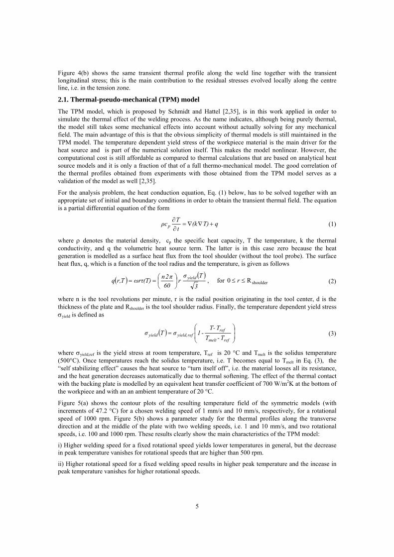
Figure 4(b) shows the same transient thermal profile along the weld line together with the transient longitudinal stress; this is the main contribution to the residual stresses evolved locally along the centre line, i.e. in the tension zone.

2.1. Thermal-pseudo-mechanical (TPM) model

The TPM model, which is proposed by Schmidt and Hattel [2,35], is in this work applied in order to simulate the thermal effect of the welding process. As the name indicates, although being purely thermal, the model still takes some mechanical effects into account without actually solving for any mechanical field. The main advantage of this is that the obvious simplicity of thermal models is still maintained in the TPM model. The temperature dependent yield stress of the workpiece material is the main driver for the heat source and is part of the numerical solution itself. This makes the model nonlinear. However, the computational cost is still affordable as compared to thermal calculations that are based on analytical heat source models and it is only a fraction of that of a full thermo-mechanical model. The good correlation of the thermal profiles obtained from experiments with those obtained from the TPM model serves as a validation of the model as well [2,35].

For the analysis problem, the heat conduction equation, Eq. (1) below, has to be solved together with an appropriate set of initial and boundary conditions in order to obtain the transient thermal field. The equation is a partial differential equation of the form

qT)(ktTρcp +∇∇=∂∂ (1)

where ρ denotes the material density, cp the specific heat capacity, T the temperature, k the thermal conductivity, and q the volumetric heat source term. The latter is in this case zero because the heat generation is modelled as a surface heat flux from the tool shoulder (without the tool probe). The surface heat flux, q, which is a function of the tool radius and the temperature, is given as follows

( ) ( )3

Tσr

60π2nωrτ(T)Tr,q yield⎟⎠⎞

⎜⎝⎛== , for shoulderR0 ≤≤ r (2)

where n is the tool revolutions per minute, r is the radial position originating in the tool center, d is the thickness of the plate and Rshoulder is the tool shoulder radius. Finally, the temperature dependent yield stress σyield is defined as

( ) ⎟⎟⎠

⎞⎜⎜⎝

⎛=

refmelt

refref yield,yield T-T

TT--1σTσ (3)

where σyield,ref is the yield stress at room temperature, Tref is 20 °C and Tmelt is the solidus temperature (500°C). Once temperatures reach the solidus temperature, i.e. T becomes equal to Tmelt in Eq. (3), the “self stabilizing effect” causes the heat source to “turn itself off”, i.e. the material looses all its resistance, and the heat generation decreases automatically due to thermal softening. The effect of the thermal contact with the backing plate is modelled by an equivalent heat transfer coefficient of 700 W/m2K at the bottom of the workpiece and with an an ambient temperature of 20 °C.

Figure 5(a) shows the contour plots of the resulting temperature field of the symmetric models (with increments of 47.2 °C) for a chosen welding speed of 1 mm/s and 10 mm/s, respectively, for a rotational speed of 1000 rpm. Figure 5(b) shows a parameter study for the thermal profiles along the transverse direction and at the middle of the plate with two welding speeds, i.e. 1 and 10 mm/s, and two rotational speeds, i.e. 100 and 1000 rpm. These results clearly show the main characteristics of the TPM model:

i) Higher welding speed for a fixed rotational speed yields lower temperatures in general, but the decrease in peak temperature vanishes for rotational speeds that are higher than 500 rpm.

ii) Higher rotational speed for a fixed welding speed results in higher peak temperature and the incease in peak temperature vanishes for higher rotational speeds.

5

iii) The gradients in thermal profiles along the transverse direction of the plate become higher with increasing welding speed, while more uniform and wider thermal profiles are obtained for the lower welding speeds.

Figure 5. (a) Contour plots of the temperature fields for rotational speed of 1000 rpm for each traverse welding speed of 1mm/s (top) and 10mm/s (bottom), respectively.

Figure 5. (b) Temperature profiles for different process variables along transverse direction

2.2. Mechanical model

For evaluation of residual stress fields, a standard mechanical model based on the solution of the static force equilibrium equations is used [36-38], i.e., one solves

0pσ jiij, =+ (4)

where pj is the body force at any point within the plate and σij is the stress tensor. The well-known Hooke’s law and a linear decomposition of the strain tensor as well as small strain theory are applied:

)u(u21ε

εεεε

εEεδδν21

ν)δδδ(δ21

ν1Eσ

ij,ji,kl

thkl

plkl

elklkl

elkl

elijkl

elklklijjkiljlikij

+=

++=

=⎭⎬⎫

⎩⎨⎧

−++

+=

(5)

The plastic strain is based on standard J2-flow theory with a temperature dependent yield surface. The conditions during yielding are described by the associated flow rule that consists of the von Mises yield surface and the consistency condition, i.e.

plij ij

pl ple e e Y e

pl plij e ij epl

ij e

ε λs

f(σ ,ε ,T) σ σ (ε ,T) 0f f ff f(s ,ε ,T) s ε ` Ts ε T

=

= − ≤

∂ ∂ ∂= = + +

∂ ∂ ∂

&&

& & && & 0=

(6)

This material description is considered to be adequate for the FSW simulation where the first order effect is the yield strength of the material as a function of temperature.

6

Figure 6. (a) Contour plot of the longitudinal stress field with increments of 22 MPa.

Figure 6. (b) Residual normal stress in longitudinal direction as a function of distance from weld line

Figure 6(a) shows the contour plots of the resulting longitudinal stress field of the symmetric models (isotherms in 25 MPa) for a chosen welding speed of 1 mm/s and 10 mm/s, respectively, for a rotational speed of 1000 rpm. A parameter study regarding longitudinal stress profiles along the transverse direction and at the middle of the plate with two welding speeds, i.e. 1 and 10 mm/s, and two rotational speeds, i.e. 100 and 1000 rpm, is presented in Figure 6(b). These results clearly show the main characteristics of the model of the residual stresses in the FSW process:

i) Higher welding speed for a fixed rotational speed results - in general - in higher stress levels in the tension zone.

ii) Higher rotational speed for a fixed welding speed yields lower peak residual stress.

iii) The gradients in residual stress profiles along the transverse direction of the plate become higher with increasing welding speed, while the model results in wider residual stress profiles for lower welding speeds.

3. Optimization Methodology In the following sections we present a study of two multi-objective optimization problems in the FSW process. These consider the minimization of the residual stresses in the workpiece together with the maximization of the production efficiency (reducing welding time and wear path), respectively. These two objectives are conflicting and techniques to deal with this issue are also considered.

The optimization procedure, which includes process integration of the ANSYS software and the optimization algorithm (NSGA-II), is handled by applying modeFRONTIER. The optimization cycle is initiated by creating an initial population of 16 pre-chosen Design-of -Computational-Experiments (DOE), for the considered process variables, i.e. the tool rotational speed (revolutions per minute), n, and the traverse welding speed, uweld. The FSW thermal and mechanical simulations, which are built by using APDL in ANSYS, are coupled in a sequential way by execution of parametric input files in a batch mode. The design variables are updated by the optimization algorithm and are read by the thermal analysis. Then the peak temperature obtained at the end of the welding session is saved in order to be used as a thermal constraint together with the transient temperature field results in order to yield the thermal strains for the mechanical analysis. The mechanical analysis gives as a result the maximum longitudinal stress value at the middle of the plate in the transverse direction, and this is used as an objective to be minimized. This optimization cycle run until the stopping criterion, i.e. the total number of generations, is reached. The flow chart of the optimization procedure is shown in Figure 7.

7

Figure 7. Flow chart of the optimization problem Figure 8. Design and objective space associated with multi-objective optimization problem

3.1. Multiobjective Optimization (MOO) Problem

Most engineering design activities require a solution of multi-disciplinary and multiobjective optimization (MOO) problems which usually deal with conflicting design objectives. The consideration of multiple conflicting objectives results in a number of alternative trade-offs, called Pareto-optimal solutions, of which none can be said to be better than any other without any additional information about the problem under consideration. This concept can be formulated as follows

(∀i fi(x) ≤ fi(y))∩(∃ j : f j(x) < f j(y)) (7)

where fi is the i-th objective function in the feasible region and the minimization of the two-objective problem, which is schematically shown in Figure 8, is considered for convenience. In this context, Eq. (7) describes that at least in one objective, design x is better than design y, while in others they might be equal; this can also be expressed as the solution x dominates the solution y in the parlance of MOO. Since the concept of domination allows a way to compare solutions with multiple objectives, most MOO algorithms use this domination concept to search for non-dominated solutions, i.e. the ones that constitute the Pareto-front [39-41]. Population-based evolutionary algorithms have in the last decade become more and more popular as they effectively can utilize distributed computing facilities. Also, they are typically able to provide a larger spectrum of Pareto-optimal solutions without any additional problem specification. The availability of trade-off solutions, representing varying preference levels between chosen objectives, makes it easier for a decision-maker to choose a particular solution for implementation [39-41].

3.2. Nondominated Sorting Genetic Algorithm (NSGA-II)

NSGA-II is a multi-objective evolutionary algorithm (MOEA) proposed by Deb et al [42], which enables finding well-spread multiple Pareto-optimal solutions for a MOO problem by incorporating three substantial features, i.e., elitism, non-dominated sorting, and diversity preserving mechanism. Elitism, which is a genetic operator used to preserve the good solutions through the generations, is also shown to increase the convergence speed of a MOEA [43].

8

Figure 9. (a) The crowding distance calculation [42] Figure 9. (b) Schematic view of the NSGA-II procedure. (From Deb et al., [42])

The preservation of well-distributed (diverse nondominated) solutions is maintained by the crowding distance operator. The crowding distance, which is calculated frontwise, is a measure of how close an individual is to its neighbors. In order to get an estimate of the density of solutions surrounding a particular solution in the population, the average distance of two points on either side of this point along each of the objectives is calculated. This quantity di serves as an estimate of the perimeter of the cuboid formed by using the nearest neighbors as the vertices. A schematic view of the procedure for the computation of the crowding distance for an ith individual is represented in Figure 9a, and formulated as

minm

maxm

)(Im

)(Im

ii ffffdd

m1i

m1i

−−

+=−+

, for i=2, …,l-1 (8)

where I(i) is the solution index of the ith individual in the (worse order) sorted list, m is the number of objectives, l is the number of the individuals in that particular front. The first and the last individual is assigned an infinite distance in order to emphasize their fitness. A large average crowding distance will result in better diversity in the population.

The schematic view of NSGA-II on a flowchart is shown in Figure 9b. The procedure starts with an initialization of the parent population, P0, followed by sorting the members of the population based on nondomination into each front, Fi. Each individual is assigned two fitness values, i.e. the one related to its nondomination level (front or rank, i.e. Fi refers to front with rank i in Figure 9) and the crowding distance. Parents are selected by using binary tournament selection based on these two measures. An individual is selected if its rank is less than the other, since the minimization is assumed, or if the crowding distance is greater than the other. The selected population generates off-springs, Qt, by the application of usual genetic operators, i.e. crossover, mutation, etc. [44]. Since all the parent and the offspring individuals are included in the combined population, Rt, elitism is ensured. In order to reduce the size of the population of the next generation from 2N to N, nondomination sorting is applied and the individuals with relatively lowest possible ranks are accomodated until the size of the population exceeds N. Then the individuals in front Fi are selected based on their crowding distance. This cycle is repeated until the stopping criterion, i.e. the total number of generations, is met. For details, please consult the original study [42].

3.3. Problem Statement-1

The first optimization problem here is stated as the goal of finding the friction stir welding process parameters, i.e. tool rotation speed and traverse welding speed, which provide a set of trade-off solutions for the minimization of two conflicting objectives. These are the residual stresses, which are measured at the middle of the plate along the transverse direction, and the welding time that can also be stated equally as the maximization of the traverse welding speed. The optimization problem is constrained by the process-specific thermal constraints, which are given as the upper and the lower bounds on the peak temperatures in

9

the workpiece. The lower bound of 420°C on the peak temperature represents the need for easy traversing of the tool, i.e. to minimize the tool loads along the weld line by contributing to thermal softening of the workpiece material. The upper bound of 480°C is defined in order to consider the tool life and the workpiece properties which are affected by hot welding conditions. This constrained multi-objective problem can then be expressed in mathematical terms as

Minimize: f1(x) = σx,max

Maximize: f2(x) = uweld

subject to: g1(x) = 420°C ≤ Tpeak

g2(x) = Tpeak ≤ 480°C

(rpm) 1000 ..., 200, 100,n(mm/s) 10 ..., 2, 1,u

,n

ux weldweld

==

⎭⎬⎫

⎩⎨⎧

=

(9)

where x represents the design variable vector, i.e. uweld, the traverse welding speed that is changing from 1 mm/s to 10 mm/s in 1 mm/s increments and n, the tool rotational speed which varies from 100 rpm to 1000 rpm in 100 rpm increments (this results in 10 discrete values in each design variable), σx,max defines the peak longitudinal stress, and Tpeak is the peak temperature in the workpiece.

3.4. Problem Statement-2

The second optimization problem, which is a slightly modified version of the first case, considers the minimization of the so-called wear path of an arbitrary point on the tool shoulder, and it also takes the minimization of the residual stresses on the workpiece into account:

Minimize: f1(x) = σx,max

Minimize: f2(x) = ω/uweld

subject to: g1(x) = 420°C ≤ Tpeak

g2(x) = Tpeak ≤ 480°C

(rpm) 1000 ..., 200, 100,n(mm/s) 10 ..., 2, 1,u

nu

x weldweld

==

⎭⎬⎫

⎩⎨⎧

= ,

(11)

The wear path at the radius r at any point on the tool/workpiece interface can be approximated by the following expression,

weldweldweld

weld

weldweldweldcircumfpath u

ωCuω)(rL

uLωrωrttvL ===== (10)

where C is a parameter that will remain constant for the point under consideration. Minimization of the ratio of rotational speed/welding speed corresponds to maximizing the tool advance per revolution. Other studies (described below) have found weld property variations as a function of either welding speed/rotational speed, i.e. the weld pitch, rotational speed/welding speed or pseudo heat index. However, none of these are based on an argumentation addressing the wear criterion as presented in this paper, neither are they used for optimization purposes, but more for process characterization and understanding.

In the literature it has been reported that, in general, the specific weld energy (Joules/meter) correlates with the weld pitch, i.e. the energy per unit length of weld increases as the weld pitch decreases [45]. The peak temperature in the weld zone increases with an increase in the ratio of tool rotation rate/traverse speed [46]. The recrystallized grain size is reduced by decreasing the ratio of tool rotation rate/traverse speed which then results in an increase in both the degree of deformation and the peak temperature of the thermal cycle [47]. In [48], the pseudo-heat index (w=ω2/uweld) was used as part of a generalized relationship in order to find the peak temperature for several aluminum alloys. It was found that an increase in the ratio of rotational speed/traverse speed (ω/uweld) leads to a slight decrease in yield and ultimate strength of the stir

10

zone and transitional zone. It was also observed that increasing this ratio increases the weld nugget size and decreases the incomplete root penetration [49].

4. Results The initial population for the NSGA-II algorithm that is used for both cases is chosen as a modified Full Factorial Design with 4-levels (n: 100, 400, 700, 1000 rpm and uweld: 1, 4, 7, 10mm/s) resulting totally in 16 designs. The crossover and the mutation probabilities of 0.9 and 1.0, respectively, are chosen for running a total of 20 generations giving in total a number of 320 solutions.

4.1. Results of the 1st Problem Statement

The solution of the first optimization case, which is defined in section 3.1, is presented in both the design and the criterion space in the following figures. Some of the designs out of a total of 320 designs are overlapping due to relatively coarse discretization of the chosen design variables and also the selection operator. This lies in the nature of the genetic algorithm that implies the survival of some designs without evolution. Figure 10(a) and 10(b) represent feasible and unfeasible designs with dark and fair colors, respectively; constituting 49 different design points out of 100 (we use a 10x10 discretization). The surface in each figure, i.e. the peak temperature and the peak residual stress, is constructed by 16 DOE points which are evaluated as an initial population for NSGA-II. It can be clearly seen from these figures that the feasible region, which can also be called the robust process parameter region in this case, is defined by n-values in the interval between 200 and 400 rpms. Due to the random evolution strategy of EA, some of the feasible solutions (4, 6, 8 mm/s with 200, 300 and 400 rpms), are missing but the quality of these can be estimated from the surrounding solutions which are positioned on a linear varying region. Although the coarse discretization results in few missing solutions, it is advantageous for having an overall idea regarding the optimal feasible process frame with a moderate computational cost. In addition to this, the purpose of this study is to focus on the optimization methodology to find and discuss alternative trade-off solutions for minimization of welding residual stresses, otherwise not to conclude precise values. Having such solutions provides the engineer or manufacturer practical insight about the relationship among process variables corresponding to the Pareto-optimal solutions.

Figure 10. (a) Peak Temperature vs. design variables Figure 10. (b) Residual stress vs. design variables

The objective space that is constructed by minimization of the residual stresses and maximization of the welding speed is shown in Figure 11(a). Most of the designs lie close to the Pareto-front, which is shown in Figure 11(b). This is due to the low sensitivity of the n parameter on the residual stresses as defined in the underlying thermal model, i.e. the TPM model for a given welding speed. If the minimum-residual stress solution is emphasized for the MOO problem, i.e. choosing weightings of 1.0 for the objective of minimum-residual stress and 0.0 for the objective of maximum-welding speed, the combination of 1mm/s and 400rpm would be chosen. If the other extreme solution, i.e. with opposite weightings, is considered, the combination of 10mm/s and 400rpm would be preferred. In the case where one is looking for a 70-30%

11

trade-off solution for the same objectives, respectively, it is not clear how to estimate the optimal combination of the process variables. Due to this desired preference in objectives, the solution would be expected to be more similar to the minimum residual stress solution than the maximum welding speed. It is important to note that there are some different solutions satisfying such trade-off, but there is only one which is the optimum, i.e. 4mm/s and 400rpm in this case. In other words, that solution makes the optimum trade-off, meaning that for a particular amount of sacrifice in one objective, the optimum solution will correspond to the maximum gain in the other objective [41].

Figure 11. (a) Objective Space of the solution Figure 11. (b) Pareto Set of the solution

All Pareto-optimal solutions correspond to the maximum feasible rotational speed of 400rpm while having different welding speeds varying from 1 mm/s to 10 mm/s. The Pareto-front shown in Figure 11(b) gives an idea of ranking the alternative trade-off solutions depending on the available working conditions. If a manufacturer is able to use a standard milling machine instead of an advanced FSW machine and can afford using simple tool designs with low welding speed, he would probably not dare to go from 1 to 7mm/s in welding speed because the residual stresses yielded per unit increment in welding speed would cost higher comparing to those at higher welding speeds. The amount of sacrifice of the manufacturer relatively depends on the welding speed while one can keep the rotation speed between 200 and 400 rpms.

4.2. Results of the 2nd Problem Statement

The second optimization case defined in section 3.2 is presented below in objective space only since the design domain is kept constant while the solutions of the first optimization case are rearranged by taking the tool rotational speed into account as shown in Figure 12(a, b).

From the Pareto front in Figure 12(b) it is seen that at high welding speeds the second objective, i.e. minimum wear path, becomes dominant, whereas for low welding speeds the first objective of minimum residual stress is dominant.

It is also interesting to note that the wear path criterion divides the parameter space into two intervals based on whether the welding speed is higher or lower than 5 mm/s. Thus, it is seen on Figure 12(b) that for welding speeds above this value the Pareto solutions all have a rotational speed of 200 rpm, whereas for welding speeds below this value the rotational speed varies between 200 and 400 rpm. So, as compared to the previously found solutions, which are listed in section 4.1, the rotational speed is reduced from 400 rpm to 200 rpm at high welding speeds resulting in a slightly higher sacrifice in the first objective, i.e. minimization of the residual stresses.

12

Figure 12. (a) Objective Space of the solution Figure 12. (b) Pareto Set of the solution

The discussion for the first problem case can be seen to hold for this case as well. The single optimum solution for the lowest welding speed is kept the same, i.e. being combined with a rotational speed of 400 rpm again, while the single optimum solution for the highest welding speed is rearranged in a way that it is combined with the lowest feasible rotational speed, i.e. 200 rpm.

5. Conclusion and Discussions In this work a multi-objective optimization application for the FSW process has been presented. Two cases have been considered in which minimization of the residual stresses have been performed in combination with a maximization of the welding speed and a minimization of the wear path, respectively. The tool rotational speed and the traverse welding speed has been used as design variables. In addition to the description of the process goals, process-specific thermal limitations have been added to the optimization problem in order to take the tool loads and tool life issues into account; this has been formulated in terms of lower and upper bounds on the peak temperature. The results show that a tool rotation speed of 400 rpm is desired for the first problem while 200 rpm is preferred in general for the second case. The second optimization case definitely shows that the problem of minimization of the residual stresses can not be considered independently of the tool traversing speed, which is expected. Depending on the Pareto designs, ranking of the trade-off solution alternatives has been discussed in addition to looking at the optimization problem from a manufacturer point of view.

One could discuss whether it is enough to run 20 generations while having a population size of 16, resulting in a total of 320 design combinations in order to find the true Pareto-optimal solutions. It can be clearly seen that the feasible region is almost fully covered but in case of “what-if” studies it would not be sufficient. Then it could also be argued whether making enumeration makes sense for these highly demanding analyses. In this preliminary optimization study, the design variables are roughly discritized in order to obtain a general overview before going deep into the complex nature of the modeling and resulting optimization studies. The main focus is on finding a methodology to optimize process variables, i.e. welding speed and rotational speed, for multiple objectives under process related constraints.

The heat generation results at high traverse welding speeds are probably not estimated with high enough fidelity as only the thermal effect is taken into account; rather one should consider the highly complex phenomena in the mechanical deformation field as investigated in [50]. At higher welding speeds, e.g. 10mm/s, there might be a need for higher rotational speeds in order to avoid cold weld conditions.

It should be emphasized that since this is a preliminary study of an MOO problem regarding residual stresses in FSW, microstructural changes due to the thermal history have not been included yet. This is of course a limitation of the model since the microstructural evolution determines the final mechanical properties of the weld and in turn the service load performance of the part.

13

Another issue of the model that could be discussed is the the objective of minimization of the peak residual stress. It might be more relevant to use the “shrinkage force”, which can be evaluated as the integration of the area under the residual longitudinal stress profile in tension along the transverse direction of the work piece. This way, the width and the gradients of the stress profile in the tension zone would be taken into account also, resulting in a more relevant optimization problem seen from an industrial view point.

Despite these limitations, the procedure put forward is generic and it would be manageable to include for example the microstructures and the shrinkage force in the analysis.

6. References [1] Mishra, R.S., Ma, Z.Y., Friction stir welding and processing, Materials Science and Engineering R, Vol. 50, 2005, pp. 1-78 [2] Schmidt, H., Hattel, J., Thermal modelling of friction stir welding, Scripta Materialia, 58, 2008, pp. 332-337 [3] Schmidt, H., Hattel, J., Modelling heat flow around tool probe in friction stir welding, Science and Technology of Welding and Joining, Vol. 10, No. 2, 2005, pp. 176-186 [4] Zhu, X.K., Chao, Numerical simulation of transient temperature and residual stresses in friction stir welding of 304L stainless steel, Journal of Materials Processing Technology, Vol. 146, 2004, pp. 263-272 [5] Chao,Y.J., Qi, X., Thermal and Thermo-Mechanical Modeling of Friction Stir Welding of Aluminum Alloy 6061-T6, Journal of Materials Processing & Manufacturing Science, Vol. 7, 1998, pp. 215-233 [6] Song, M., Kovacevic, R., Thermal modeling of friction stir welding in a moving coordinate system and its validation, International Journal of Machine Tools & Manufacture, Vol. 43, 2003, pp. 605-615 [7] Chen, C.M., Kovacevic, R., Finite element modeling of friction stir welding – thermal and thermomechanical analysis, Journal of Machine Tools & Manufacture, Vol. 43, 2003, pp. 1319-1326 [8] Hattel, J.H., Schmidt, H.B., Tutum, C.C., Thermomechanical modelling of Friction Stir Welding, 8th International Conference on Trends in Welding Research Conference, ASM, June 2008. [9] James, M.N., Hughes, D.J., Chen, Z., Lombard, H., Hattingh, D.G., Asquith, D., Yates, J.R., Webster, P.J., Residual stresses and fatigue performance, Engineering Failure Analysis, Vol. 14, 2007, pp. 384-395 [10] Bussu, G., Irving, P.E., The role of residual stress and heat affected zone properties on fatigue crack propagation in friction stir welded 2024-T351 aluminum joints, International Journal of Fatigue, Vol. 25, 2003, pp. 77-88. [11] Murphy, A., McCune, W., Quinn, D., Price, M., The characterization of friction stir welding process effects on stiffened panel buckling performance, Thin-Walled Structures, Vol. 45, 2007, 339-351 [12] Bhide, B., Michaleris, P., Posoda, M., DeLoach, J., “Comparison of Buckling Distortion Propensity for SAW, GMAW, and FSW”, Welding Journal, 2006, 189-195. [13] Richards, D.G., Pragnell, P.B., Williams, S.W., Withers, P.J., Global mechanical tensioning for the management of residual stresses in welds, Materials Science and Engineering A, Vol. 489, 2008, pp. 351-362 [14] Richards, D.G., Prangnell, P.B., Withers, P.J., Williams, S.W., Nagy, T., Morgan, S., Simulation of the Effectiveness of Dynamic Cooling for Controlling Residual Stresses in Friction Stir Welds, 7th International Symposium Friction Stir Welding, TWI, May 2008 [15] Bastier, A., Maitournam, M.H., Roger, F., Dang Van, K., Modelling of the residual state of friction stir welded plates, Journal of Materials Processing Technology, Vol. 200, 2008, pp. 25-37 [16] Feng, Z., Wang, X., David, S.A., Sklad, P., Modeling of residual stresses and property distributions in friction stir welds of aluminum alloy 6061-T6, Science and Technology of Welding & Joining, Vol. 12, No. 4, May 2007 , pp. 348-356(9) [17] Altenkirch, J., Steuwer, A., Peel, M., Richards, D.G., Withers, P.J., The effect of tensioning and sectioning on residual stresses in aluminum AA7749 friction stir welds, Materials Science and Engineering A, Vol. 488, 2008, pp.16-24 [18] Steuwer, A., Peel, M.J., Withers, P.J., Dissimilar friction stir welds in AA5083-AA6082: The effect of process parameters on residual stress, Materials Science and Engineering A, Vol. 441, 2006, pp. 187-196 [19] Sutton, M.A., Reynolds, A.P., Wang, D.-Q., Hubbard, C.R., A Study of Residual Stresses and Microstructure in 2024-T3 Aluminum Friction Stir Butt Welds, Journal of Engineering Materials and Technology, Vol. 124, 2002, pp. 215-221

14

[20] Peel, M., Steuwer, A., Preuss, M., Withers, P.J., Microstructure, mechanical properties and residual stresses as a function of welding speed in aluminum AA5083 friction stir welds, Acta Materialia, Vol. 51, 2003, pp. 4791-4801 [21] Khandkar, M.Z.H., Khan, J.A., Reynolds, A.P., Sutton, M.A., Predicting residual thermal stresses in friction stir welded metals, Journal of Materials Processing Technology, Vol. 174, 2006, pp. 195-203 [22] Tutum, C.C., Schmidt H.B. Hattel, J, Assesment of Benchmark Cases for modeling of Residual stresses and Distortions in Friction Stir Welding, 7th International Symposium Friction Stir Welding, TWI, May 2008 [23] Murugananth, M., “Metaheuristic Multiobjective Optimization in Steel Welds”, Materials and Manufacturing Processes, Vol. 24, No. 2, 2009, pp. 230-239 [24] Mishra, S., DebRoy, T., Tailoring gas tungsten arc weld geometry using a GA and a NN trained with convective heat flow calculations, Materials Science and Engineering A, Vol. 454–455, 2007, pp. 477–486 [25] Michaleris, P., Dantzig, J., Tortorelli, D., Minimization of welding residual stress and distortion in large structures, Welding Journal, Vol. 78, 1999, pp. 361-366 [26] Bogomolny, M., Bendsøe, M.P., Some Optimal Design Aspects of Resistance Welding, 7th World Congress on Structural and Multidisciplinary Optimization, Seoul, May 2007, pp. 2687-2695 [27] Nandan, R., Lienert, T.J., DebRoy, T., Toward reliable calculations of heat and plastic flow during friction stir welding of Ti-6Al-4V alloy, Int. J. Mat. Res., Vol. 99, No. 4, 2008, pp. 434-444 [28] Tutum, C.C., Schmidt, H.B., Hattel, J.H., Optimization of the Process Parameters for Controlling Residual Stress and Distortion in Friction Stir Welding, International Conference on Simulation Based Engineering and Sciences, TCN CAE 2008 [29] Fratini, L., Corona, V., Friction Stir Welding Lap Joint Resistance Optimization Through Gradient Techniques, Journal of Manufacturing Science and Engineering, Vol. 129, 2007, pp. 985-990 [30] Lombard, H., Hattingh, D.G., Steuwer, A., James, M.N., Optimising FSW process parameters to minimise defects and maximise fatigue life in 5083-H321 aluminum alloy, Engineering Fracture Mechanics, Vol. 75, 2008, pp. 341-354 [31] Lakshminarayanan, A.K., Balasubramanian, V., Process parameters optimization for friction stir welding of RDE-40 aluminum alloy using Taguchi technique, Trans. Nonferrous Met. Soc. China, Vol. 18, 2008, pp. 548-554 [32] Tutum, C.C., Schmidt, H., Hattel, J., Bendsøe, M., Estimation of the Welding Speed and Heat Input in Friction Stir Welding using Thermal Models and Optimization, 7th World Congress on Structural and Multidisciplinary Optimization, Seoul, May 2007, pp. 2639-2646 [33] Larsen, A.A., Bendsøe, M.P., Schmidt, H.N.B., Hattel, J.H., Optimization of Thermal Aspects of Friction Stir Welding – Initial Studies Using a Space Mapping Technique, 7th World Congress on Structural and Multidisciplinary Optimization, Seoul, May 2007, pp. 2663-2669 [34] Zhu, X.K., Chao, Y.J., Effects of temperature-dependent material properties on welding simulation, Computers and Structures, Vol. 80, 2002, pp. 967-976 [35] Schmidt, H.B., Hattel, J.H., A thermal-pseudo-mechanical model for the heat generation in Friction Stir Welding, 7th International Symposium Friction Stir Welding, TWI, May 2008 [36] Lindgren, L.-E., “Computational Welding Mechanics: Thermomechanical and Microstructural Simulations”, Woodhead Publishing Ltd, 2007 [37] Labeas, G., Tsirkas, S., Diamantakos, J., Kermanidis, A., “Effect of residual stresses due to laser welding on the Stress Intensity Factors of adjacent crack”, 11th International Conference on Fracture, March 2005 [38] Nadimi, S., Khoushehmehr, R.J., Rohani, B., Mostafapour, A., “Investigation and Analysis of Weld Induced Residual Stresses in Two Dissimilar Pipes by Finite Element Modeling”, Journal of Applied Sciences, Vol. 8, No. 6, pp. 1014-1020 [39] Deb, K., Multi-Objective Optimization Using Evolutionary Algorithms, John Wiley & Sons, 2001 [40] Deb, K., Multi-objective Genetic Algorithms: Problem Difficulties and Construction of Test Problems, Evolutionary Computation, Vol. 7, No. 3, 1999, pp. 205-230 [41] Deb, K., Unveiling innovative design principles by means of multiple conflicting objectives, Engineering Optimization, Vol. 35, No. 5, 2003, pp. 445-470 [42] Deb, K., Pratap, A., Agarwal, S., Meyarivan, T., A Fast and Elitist Multiobjective Genetic Algorithm: NSGA-II, IEEE Transactions on Evolutionary Computation, Vol. 6, No. 2, 2002, pp. 182-197 [43] Zitzler, E., Deb, K., Thiele, L., Comparison of multiobjective evolutionary algorithms: Emprical results, Evolutionary Computation, Vol. 8, No. 2, 2000, pp. 173-195

15

[44] Goldberg, D.E., Genetic Algorithms in Search, Optimization, and Machine Learning, Addison-Wesley, 1989 [45] Seidel, T.U., Reynolds, A.P., Visualization of the Material Flow in AA2195 Friction-Stir Welds Using a Marker Insert Technique, Metallurgical and Materials Transactions A, Vol. 32A, 2001, pp. 2879-2884 [46] T. Hashimoto, S. Jyogan, K. Nakata, Y.G. Kim, M. Ushio, FSW joints of high strength aluminum alloy, Proceedings of the First International Symposium on Friction Stir Welding, Thousand Oaks, CA, USA, June 14–16, 1999 [47] Ma, Z.Y., Mishra, R.S., Mahoney, M.W., Superplastic deformation behaviour of friction stir processed 7075Al alloy, Acta Materialia, Vol. 50, No. 17, 2002, pp. 4419-4430 [48] W.J. Arbegast, P.J. Hartley, Friction Stir Weld Technology Development at Lockheed Martin Michoud Space System-An Overview, Proceedings of the Fifth International Conference on Trends inWelding Research, Pine Mountain, GA, USA, June 1–5, 1998, p. 541 [49] Gharacheh, M.A., Kokabi, A.H., Daneshi, G.H., Shalchi, B., Sarrafi, R., The influence of the ratio of “rotational speed/traverse speed” (w/v) on mechanical properties of AZ31 friction stir welds, International Journal of Machine Tools & Manufacture, Vol. 46, 2006, pp. 1983-1987 [50] Schmidt, H., Hattel, J., A local model for the thermomechanical conditions in friction stir welding, Modelling Simul. Mater. Sci. Eng., Vol. 13, 2005, pp. 77-93

16

D PAPER-IV

J. H. Hattel, H. N. B. Schmidt and C. C. Tutum, "Thermomechanical Modelling of Fric-

tion Stir Welding", Proc. 8th International Conference on Trends in Welding Research,Pine Mountain, Atlanta, USA, 2008 (Invited keynote lecture).

147

Thermomechanical Modelling of Friction Stir Welding

J.H. Hattel, H.N.B. Schmidt and C. Tutum Department of Mechanical Engineering

Technical University of Denmark DK-2800 Lyngby, Denmark

Abstract

Friction Stir Welding (FSW) is a fully coupled thermomechanical process and should in general be modelled as such. Basically, there are two major application areas of thermomechanical models in the investigation of the FSW process: i) Analysis of the thermomechanical conditions such as e.g. heat generation and local material deformation (often referred to as flow) during the welding process itself. ii) Prediction of the residual stresses that will be present in the joint structure post to welding. While the former in general will call for a fully-coupled thermomechanical procedure, however, typically on a local scale, the latter will very often be based on a semi-coupled, global procedure where the transient temperatures drive the stresses but not vice-versa. However, in the latter, prior knowledge about the heat generation must be obtained somehow, and if experimental data are not available for the FSW process at hand, the heat generation must either be prescribed analytically or based on a fully coupled analysis of the welding process itself. Along this line, a recently proposed thermal-pseudo-mechanical model is presented in which the temperature dependent yield stress of the weld material controls the heat generation. Thereby the heat generation is still numerically predicted but the cumbersome fully coupled analysis avoided. In the present work the formulation of all three mentioned modelling approaches as well as the very fundamental pure thermal models are briefly presented and discussed together with selected modelling results including prediction of material flow during welding, prediction of heat generation with the thermal-pseudo mechanical model as well as residual stress and deformation analysis combined with in-service loads.

Introduction

During the last decade an increasing amount of contributions have been given in literature in the field of thermomechanical modelling of FSW. These models are generally chategorized by either their area of application, i.e. flow models or residual stress models, or by the continuum mechanics approach they

are based upon, i.e. Computational Solid Mechanics (CSM) models or Computational Fluid Dynamics (CFD) models, where the former typically are Lagrangian and the latter Eulerian, see figure 1.

Figure 1: Left: Lagrangian model of FSW. Right: Eulerian model of FSW, [1].

The equations for conservation of momentum, energy and mass, respectively are in the Lagrangian and Eulerian frames given by

Table 1: Governing equations for conservation of momentum, energy and mass, respectively in Lagrangian and Eulerian frames.

Lagrangian frame Typically CSM

Eulerian frame Typically CFD

Energy

, ,pl

p i ij ijic T kT s , ,,

( )plp i ij ij i p ii

c T kT s u c T

Momentum ,i ji j iu p , ,( )i ji j i j i ju t p u u

MassNo explicit equation iiu ,)(

These are the fundamental, governing partial differential equations that depending on the continuum mechanical framework that is used will need to be modified and combined with proper constitutive laws for the particular case at hand. In the following, the basis of thermal models, computational solid mechanics (CSM) models, computational fluid dynamics (CFD) models and the new thermal-pseudo-

Trends in Welding Research, Proceedings of the 8th International ConferenceStan A. David, Tarasankar DebRoy, John N. DuPont, Toshihiko Koseki, Herschel B. Smartt, editors, p 1-10DOI: 10.1361/cp2008twr001

Copyright © 2009 ASM International®All rights reserved.

www.asminternational.org

1

mechanical model for FSW are shortly presented and the above shown equations are modified accordingly. It should be mentioned that although microstructural models and their coupling to mechanical properites are very important for predicting the behaviour of FSW welds, they are not discussed in the present work.

Thermal models

Thermal modelling has since the late nineties been a central part of modelling of FSW in general (some major contributions are given in [2-10] ). One of the reasons for this is that many of the properties of the final weld are directly a function of the thermal history which the workpiece has been exposed to. Secondly, the FSW process itself is highly affected by the heat generation and heat flow and thirdly, from a modelling viewpoint, thermal modelling of FSW can be considered the basis of all other models of the process, be it microstructural, CFD or CSM models. In the FSW process the welding parameters are all chosen such that the softening of the workpiece material enables the mechanical deformation and material flow. However, unlike many other thermomechanical processes, the mechanisms of FSW are fully coupled meaning that the heat generation is related to material flow and frictional/contact conditions and vice versa. Thus, in theory a thermal model alone cannot predict the temperature distribution/history without a pre-knowledge about the heat generation, since the fundamental mechanisms of FSW are not part of a pure thermal model. For this reason, several analytical expressions have been given in literature for the heat generation for a given weld as a function of tool geometry and welding parameters, e.g. tool radius and rotational speed. This means that in the energy equation in table 1, the plastic dissipation term is replaced by a heat source term, see table 2, line 1.

Table 2: Governing equations for conservation of energy in thermal models, respectively in Lagrangian and Eulerian frames

Lagrangian frame Eulerian frame Energy with source term

, ,p i ic T kT Q , , ,

0 i i pi ikT Q u c T

Energy without source term but all heat prescribed at surface

, ,p i ic T kT , , ,

0 i i pi ikT u c T

In all thermal models of FSW the main task now is to solve this energy equation with an appropriate set of initial and boundary conditions. However, in most pure thermal models of FSW, the heat generation from both frictional and plastic dissipation is modelled via a surface flux boundary condition at the tool/matrix interface, see table2, line 2. The main unknown parameters in these surface flux expressions are either the friction coefficient under the assumption of sliding and the material yield shear stress under the assumption of sticking.

Along this line, the authors have proposed the following generally adopted equation for the total heat generation, [7], (see figure 1)

3 3 3 2

1

2 13

1 tan 3

total sticking sliding

yield

shoulder probe probe probe

Q Q Q

p

R R R R H

(1)

Where is the dimensionless slip rate between the tool and the work piece (1 for full sticking and 0 for full sliding).

Figure 2: Different contributions from the shoulder and the pin to the surface heat generation, [6].

However, when implementing this into a numerical model using a position dependent surface flux [Wm-2], it is typically used on the following form, [6],

1total friction yield

yield

q r

r p (2)

which in fact is the basis for deriving equation (1). Furthermore, when combining equation (1) and (2) and assuming the simple tool geometry of a flat shoulder only, one obtains the following well-known expression for the heat generation [Wm-2], see e.g. [7],

3

32

totaltotal

shoulder

Q rqR

(3)

which can be applied as a radius dependent surface flux in the model, under the assumption of a constant contact condition close to sliding or in cases of sticking where the shear layer is very thin.

From equation (3) it can be seen that totalQ can be considered an input parameter in the same manner as the friction coefficient, the pressure and the material’s yield shear stress in equation (1). However, it should be mentioned that having

totalQ as part of the input parameters for the model in some

2

situations could conflict with the very objective for thermal modelling of FSW. This is especially the case when the model should predict temperatures for conditions not supported by measurements of the heat input totalQ . In these cases it is not straightforward to predict or simulate the effect of e.g. a change in welding or rotational speed, because the total heat generation totalQ is a function of these changes in parameters and hence can be considered an internal function of the FSW process; unlike other welding process, e.g. TIG where the heat input is controlled externally. This dilemma can of course be overcome by supporting the thermal model with a thermo-mechanical CSM or CFD based model which “includes” the underlying physics of the process, namely the material flow producing heat generation by plastic dissipation in the shear layer and frictional contact at the tool/workpiece. As being pretty obvious from the later sections on CSM and CFD models, the efforts for such simulations are highly demanding from both a computational and a human resource point of view, thus leaving pure thermal modelling of FSW as a valuable “simple” alternative for simulation of heat flow having in mind the limitation of such models, which as earlier mentioned primarily lie in the evaluation of totalQ .Having said that, it should be noted that the most utilized procedure for evaluating totalQ typically is to rely on experimental findings by simply performing the actual welds and measuring totalQ with a dynamometer, and thereby accepting the inherent limitation of the resulting thermal model to predicting only temperatures for a known total heat generation.

Since the prescribing of the heat generation is the most single important parameter in thermal models of FSW the authors proposed a classification of different heat sources [7]. One characteristic in this classification is how “detailed” the tool heat generation is resolved. Three levels were evaluated, i.e. i) including shoulder heat generation, without probe heat generation, ii) including shoulder and probe heat generation, with probe material and iii) shoulder and probe heat generation but without probe material. A second characteristic was whether the convective contribution due to the material flow in the shear layer was taken into account. Two extreme contact conditions were evaluated, i.e. full sliding and full sticking. In the case of sliding the heat was applied as a surface flux and in the case of sticking the heat was applied as a volume flux in a shear layer. This shear layer was prescribed analytically assuming a uniform thickness with a linear velocity profile ramped between the tool velocity at the contact interface and the welding velocity outside the shear layer. It was concluded that for analysing the temperature field in the volume under the tool, special attention should be paid to how the heat generation and the material “flows” around the tool probe. The main effect of including the probe in the thermal model is to change the material properties to those of the tool;

secondly, rotating the probe and modelling the shear layer around it such that it resembles a flow model.

One new procedure to obtain the heat generation is to couple the traditional analytical expression for the heat generation with a constraint based on experimental or phenomenological considerations. It is well-known from the constitutive behaviour of a solid (representative for those alloys used in FSW), that the yield stress dramatically decreases once the temperature approaches the solidus temperature. Above the solidus temperature, the material acts as a fluid. As a consequence, the material close to the tool/matrix interface will reduce its heat generation to negligible values if exceeding the solidus temperature – reducing the temperature level – allowing the material to recover its strength. A self-stabilizing effect will thus establish at a temperature level around the solidus temperature, hence this could be used as an average temperature constraint in a pure thermal model. This is what is done in the thermal model by Tutum et al. [10] where the heat generation in FSW of AA2024 is controlled by using an optimization scheme such that an averagetemperature of 500 oC at the tool/workpiece interface is obtained. This procedure has given promising results for obtaining temperature fields without prior knowledge regarding totalQ – in fact this is an output of the optimization analysis.

Computational Solid Mechanics Models

As mentioned before, the two reasons for doing solid mechanics models of FSW are to predict the flow and to predict the residual stresses. The main governing equations for these types of models are given in table 3. The energy equation will essentially be as shown in table 1, line 1 (giving a fully coupled thermomechanical model) or table 2 (giving a sequentially coupled thermomechanical model) depending on the choice of thermal model. For the solid mechanically based flow modelling there are basically two approaches: The simplest is to assume a rigid-visco-plastic material, i.e. the total strain is equal to the visco-plastic strain and use an implicit solver based on quasi-static equilibrium. This is done by several authors in literature, see e.g. [12-14]. The more comprehensive approach is to use the dynamic equilibrium equation and to take all the contributions to the strain into account although the viscoplastic part obviously is the dominating contribution. This is typically done in an ALE formulation where the dynamic equilibrium equation is solved in an explicit manner. This approach has been used by several authors, see e.g. [15-18]. A special feature about the model by Schmidt and Hattel [17] (implemented in ABAQUS Explicit) is that the heat generation between the tool and the matrix is not prescribed but part of the solution itself. This adds to the generality of the model but also to the complexity and hence the need for computational power. The model [17] has been used to predict among others the plastic strain in the weld which resembles the well-known “flow arm” quite well, see figures 3 and 4 as well as the void

3

formation behind the tool, see figure 6, being the first model in literature able to predict this.

Table 3: Basic equations for solid mechanics models of FSW for flow and residual stresses, respectively

Flow during welding Residual stresses Momentum Dynamic equilibrium, e.g. explicit ALE

,i ji j iu p

Dynamic equilibrium not relevant

Static equilibrium, e.g. implicit “flow formulation”

, 0ji j ip

Static equilibrium. Quasi-static thermomechanical analysis

, 0ji j ipStrain vs. displacements Large strain theory

1, , , ,2 ( )tot

ij i j j i k i k ju u u uSmall strain theory

1, ,2 ( )tot

ij i j j iu uTotal strain Rigid viscoplastic:

tot vpij ij

Explicit ALE tot el pl vp thij ij ij ij ij

Rate independent plasticity tot el pl thij ij ij ij

Thermal strain 2

1

( )Tth

ij ij TT dT

Constitutive lawEquivalent stress

1 232 ij ij

Equivalent total strain rate (rigid viscoplastic)

1 223

tot tot totij ij

Yield stress, in general: ( , )pl

y y T0y cut off solT T T

Norton power law m

y KInverse hyperbolic sine

111

lnln

sinh nZy A

Q RTZ e mJohnson-Cook

01 ln

1 ref

sol ref

ny

mT TT T

A B C

Equivalent stress 1 23

2 ij ij

Equivalent plastic strain 1 22

3pl pl pl

ij ij

Yield stress, in general: ( , )pl

y y T0y cut off solT T T

Hardening law, e.g. Ramberg-Osgood:

n

ytot

yE E

ElasticityHooke’s generalized law

1 1el elE

ij ij ij ij

Apart from modelling the flow, the purpose of the computational solid mechanics models of FSW obviously is to find residual stresses, see e.g. [19-22]. As seen from table 3 it is clear that these ressidual stress models typically are based on a thermo-elasto-plastic description, whereas the flow models are based on rigid-visco-plastic models in most cases.

Nugget

Flow arm

Figure 3: Micrsotructure showing the well-known “flow arm” from the nugget, [17].

Figure 4: Numerically predicted equivalent plastic strain (in the range of 0-75) showing a similar result in figure 4, [17].

Lack of contactRisk of void formation

Figure 5: Numerically predicted size of velocity. Note the lack of contact resulting in risk of void formation at the advancing side, [17].

An analysis of the residual stresses and the coupling to the subsequent load situation was carried out by the authors in ABAQUS Standard on a structure where a stringer is friction stir welded onto a plate [22], see figure 6. The integrated residual stress and load analysis consisted of four steps which are shown in figure 7. The residual stresses along the dotted line shown in figure 7 after welding and releasing as well as after applying the load are presented in figure 8. As seen on the figure, applying the load actually slightly reduces the longitudinal stresses in the middlle of the weld. This is of course not a general statement but only valid for this

4

geometry and load case. Moreover, it should be emphasized, that this type of analysis obviously would benefit a lot from a prediction of the transient evolution of the mechanical properties in the structure close to the weld.

Figure 6: Geometry of a stringer friction stir welded to a plate. Used for coupling of residual stress and in-service load analyses, [22].

Step-1 and 2: Welding & Cooling Step-3: Releasing

Step-4: Service Load

The entire boundary is clamped (All-DOF fixed)

25kg Stresses reported along this line

Figure 7: The 4 steps in the coupled residual stress and in-service load analyses, [22]

Figure 8: Longitudinal and transverse residual stresses after welding and releasing as well as after applying the load, [22].

Computational Fluid Dynamics Models

Traditionally speaking, CFD models will not be considered as being of “thermomechanical type” in computational welding mechanics. In conventional welding processes, CFD models are normally used for weld pool dynamics and CSM models for residual stresses. However, in FSW both CSM models as the ABAQUS Explicit model mentioned above [17] and CFD models as the one that will be shown in the following can be used to find the material flow during welding. For this reason it makes good sense to present the CFD approach to material flow in FSW, anyway. The basic assumption in the CFD models obviously is to treat the matrix material as a fluid, see table 4 for an overview of the governing equations. In particular, this calls for a suitable constitutive model from which the viscosity can be expressed. In literature, it is the most common for FSW to use the inverse hyperbolic sine law, see tables 3 and 4, for the yield stress as a function of the shear rate. This expression captures both the power law regime for low strain rates and the power law breakdown at higher strain rates. CFD models are typically formulated in a Eulerian frame, so that the tool is stationary, hence only rotating and the welding speed is accounted for by having incoming and outgoing material flow at the boundaries. The energy equation will be that of table 1, line 1 (right) for a fully-coupled model or table 2, lines 1 and 2 (right) for a sequentially coupled model. Some important contributions to flow modelling in FSW based on CFD can be found in [23-27]. In Figures 9 and 10, a comparison between experiment, analytically based streamlines and a CFD model (implemented in COMSOL) is shown, [28]. The experiment contained of welding through a line of Cu marker material (MM) in two plates of 2024 and then unscrewing the tool as its center was aligned with the line of MM.

Based on experimental findings in terms of CT pictures and comparisons with theoretical predictions by both analytical and numerical flow models, the authors, [28], have proposed

5

three characteristic zones for the flow around the tool probe: i) the rotation zone. ii) the transition zone and iii) the deflection zone, see Figure 11. It should be mentioned that this classification is based on a simplified representation of the real, more complex flow – thus not taking into account 3D flow effects, non-symmetrical tool features (e.g. threads) and cyclic contact condition (collapse of the shear layer).

Table 4: Basic equations for fluid mechanics models of FSW for flow

MomentumSteady state

, ,0 ( )ji j i j i jp u uSteady state, Stokes flow

,0 ji j ipStrain rates vs. displacement rates

1, ,2 ( )Tot

ij i j j iu uConstitutive lawIncompressible Newtonian

2ij ij ijPEq. stress vs. eq. strain rate

( 1)K m

Cut-off temperature 0 cut off solT T T

Incompressible non-Newtonian 2ij ij eff ijP

Eq. stress vs. eq. strain rate mK

Effective viscosity, in general 1 13

3m m

eff eff

Effective viscosity, power law 11

3m

eff KEffective viscosity, inv.hyp.sine

111 1sinh3

nQ RTA

eff

e

Cut-off temperature 0eff cut off solT T T

Figure 9: Left: CT picture of weld with transverse MM. Exit hole aligned with the MM plane. Right: Analytically obtained stream lines/tracer particles, [28].

The CFD models are very suitable for analyzing the material flow during FSW, however they have some important limitations that should be mentioned: i) The residual stresses after welding which are of great importance cannot be captured, since a CFD model in nature is rate dependent only.

ii) The elastic stress state in the area “far away” from the tool is not properly described. iii) The contact condition at the tool/interface is typically not very well described in the present CFD models of FSW, i.e. an a priori prescribed velocity emulating either sticking or sticking/sliding is normally used. These three limitations mentioned for the CFD models are all more or less eliminated if the material flow is described by computational solid mechanics models. These, on the other hand, often have the disadvantage of high demands for remeshing, which the CFD models, being of Eulerian nature, do not.

Figure 10: CFD model in COMSOL with simulated tracer particles. Non-Newtonian model with m=0.17, [28].

Figure 11: Characteristic zones for the flow around the tool probe: i) the rotation zone. ii) the transition zone and iii) the deflection zone, [28].

Thermal-pseudo-mechanical model

In this paragraph, the author’s recently proposed thermal-pseudo-mechanical model [1] is presented. As the name indicates, the model, although being purely thermal from the viewpoint of the classification presented in the present work, still takes some mechanical effects into account without actually solving for any mechanical fields. The main advantage of this is that the obvious simplicity of thermal models is still maintained in the thermal-pseudo-mechanical

6

model. The basis of the model is to consider the heat generation at a material segment which in general depends on the material flow stress for the given temperature, given strain and given strain rate. The contact stress must be in equilibrium with the material yield shear stress of the underlying material during steady state conditions. This also holds for contact conditions close to sliding, because just for the slightest degree of sticking, i.e. ~ 0 1, see [7] for definition, there will be plastic deformation at the very interface, hence equilibrium between the contact/frictional stress and the material response must prevail. For steady state conditions, this leads to the following relationship

( )friction contact yield T (4)

where interface

, ,T T x y z is the non-uniform temperature at the contact interface.

Realizing this, leads to using the material’s yield stress to describe the heat generation coming from friction rather than relying on the more classical Coulomb approach which uses the non-uniform pressure distribution and the friction coefficient which in general is a function of the temperature, slip rate, pressure and interface properties (roughness, etc.). Thus, the alternative approach proposed here quantifies the heat generation via the material’s yield stress which in general is a function of temperature, strain and strain rates.

However, since it is not the aim to involve a full thermomechanically based solution, only the temperature dependence of the material flow stress is taken into account. This leaves a very important point to be clarified: For which values of and should the yield stress be chosen? In other words: How should the mechanical history that a material segment experiences during its path through the shear layer be represented? At the present stage, the maximum values of the yield stress resembling a torsion test for a constant strain rate have been chosen.

Summing up, the benefits as compared to classical Coulomb friction are several: a) more data is available for the material’s yield response as compared to the friction coefficient b) prior knowledge to the pressure distribution is not needed c) the model becomes much more robust towards variations in the input data.

In the thermal pseudo mechanical model, the heat generation contributions from friction and plastic dissipation are now both described as a surface flux and given by

(1 )friction friction

plastic yield

q rq r

(5)

Combining these expressions with equation (4) and assuming pure shear yields

( )( )

3yield

total yield

Tq r T r (5)

which underlines the fact that the entire heat generation is modelled as a surface flux which is depending on the local temperature. This temperature dependence hence leads to a heat source which is part of the numerical solution itself, making it a non-linear problem to solve. This obviously calls for an iterative procedure. However, it turns out that the price in calculation time is relatively low, i.e. a typical thermal pseudo mechanical model needs approximately twice the calculation time as a normal steady state thermal model of FSW. It should be underlined that the above described thermal-pseudo-mechanical model will capture the first order effect of the material’s mechanical response without making a full thermomechanical model. A very important characteristic about this model is the self-stabilizing effect once temperatures reach the solidus temperature, in which case the heat source “turns itself off”. This makes the model effectively more dependent on changes in boundary conditions and welding parameters, rather than e.g. choice of material law. Moreover it should be further underlined that the heat transfer coefficients describing boundary conditions are the only fitting parameters in the model. It is important to emphasize that once these have been found, the effect of welding parameters such as welding velocity and rotational speed can be varied and the model will implicitly capture this in the heat generation and temperature profiles.

Figure 12: Shear yield stress derived from [29].

The temperature dependent heat source given by equation (5) is implemented in a Eulerian model that, in addition to the workpiece, includes the tool and the backing plate. The thermal model is implemented in Comsol 3.3 and is based on

7

an experiemental weld of 7075 T6 instrumented with thermocouples. The welding conditions are given in [1] and the thermal properties are taken from [29]. The experimentally found values for the maximal yield stress of friction stir processed 7075 at strain rates of 0.001 1/s are used for the shear yield stress in figure 12. A total of 100.000 degrees of freedom in the model are solved for. A more thorough description of the model can be found in [1]. Figure 13 shows the model results for the local heat generation given by equation (5) evaluated along the intersection between the tool and the joint line. The temperature dependent heat generation denoted by (-) is the result of the thermal-pseudo-mehcanical model and this is compared with the analytically prescribed, linearly dependent heat generation denoted by (--); the latter was evaluated using the same total heat generation as being a result of the former. In the interval under the probe tip, the heat genearation is close to linear since the temperature is nearly constant in this area.

Figure 13: Local heat generation as calculated from eq. (5) evaluated along the intersection between tool and centreline. The total heat generation in the analytical model is prescribed with the value obtained in the thermal-pseudo-mechanical model, [1].

The exponetially increasing heat generation at both the leading and trailing shoulder regions is a combination of the r-term and the increase in yield shear stress due to the decrease in temperature for larger radii (here shown as x-values). The total heat generated at the tool/matrix interface is found to be 1.9 kW (83% from the shoulder, 16% from the conical probe sides and 1% from the probe tip). Moreover, the global thermal efficiency is found to be 88%. Figure 14 shows the corresponding temperatures along the same intersection. It is very obvious that the overestimation of the temperature at the most outer region of the shoulder in the analytical model is avoided by the self-establishing turning off effect of the thermal-pseudo-mehcanical model.

Figure 15 shows a comparison between the experimentally found temperature profiles and the modelling results. The good correleation between the profiels is obtained by adjusting only the heat transfer coefficients/contact resistances. Most important in this context is the coupling between the workpiece and the backing plate.

−0.01 −0.005 0 0.005 0.01400

420

440

460

480

500

520

540

560

x−position along centerline/tool intersection [m]

Tem

pera

ture

[o C]

leading shoulder

leading probe conical side

probe tip

trailing probe conical side

trailing shoulder

Tsolidus

=532 oC

Thermal−pseudo−mechanicalAnalytically prescribed heat source

−0.01 −0.005 0 0.005 0.01400

420

440

460

480

500

520

540

560

x−position along centerline/tool intersection [m]

Tem

pera

ture

[o C]

leading shoulder

leading probe conical side

probe tip

trailing probe conical side

trailing shoulder

Tsolidus

=532 oC

Thermal−pseudo−mechanicalAnalytically prescribed heat source

Figure 14: Predicted temperatures along the intersection between tool and centreline, [1].

Figure 15: Comparison between the thermal-pseudo-machanical model and experimental results for the far-field temperature profiles at y-values of 15, 30, 45 and 60 mm, [1].

In figure 16 iso-curves for the resulting heat generation are depicted as a function of the welding speed and the rotational speed. Note that for a fixed rotational speed [rpm], increasing the welding speed [mm/s] gives an increase in the heat generation [W]. Similarly for a fixed welding speed, an increase in rotational speed gives an increase in the heat generation. This is also what one would expect.

8

100 200 300 400 500 600 700 800 900 10001

2

3

4

5

6

7

8

9

10

Rotational speed [RPM]

Wel

ding

spe

ed [m

m/s

]

2000

2000

20002500

2500

25002500

3000

3000

30003000

3500

3500

3500

4000

Figure 16: Iso-curves for the resulting heat generation [W] as a function of the welding speed [mm/s] and the rotational speed [rpm], [27].

Figure 17 depicts iso-curves for the maxiamal temperature [ºC] as a function of the rotational speed and welding speed. Here it is noticed that for a fixed rotational speed, increasing the welding speed reduces the maximal temperature and for a fixed welding speed, increasing the rotational speed gives increased maximal temperatures. Note, that the distance between the iso-curves for the maximal temperature becomes increasingly larger when increasing the rotational speed, since the temperature approaches the cut off temperature.

100 200 300 400 500 600 700 800 900 10001

2

3

4

5

6

7

8

9

10

Rotational speed [RPM]

Wel

ding

spe

ed [m

m/s

]

400

420

420

440

440

440

460

460

460

480

480

480

500

500

500

505

505

505

510

510

510

515

515

515

520

520

520

525

Figure 17: Iso-curves for the resulting maximal temperature [ºC] as a function of the welding speed [mm/s] and the rotational speed [rpm], [27].

The thermal-pseudo-mechanical model presented here is the first attempt to develop a thermal model in which the total heat generation is not an input parameter, but actually a result of the model itself. It should be strongly underlined that the good

agreement between the analytically prescribed heat source model and the thermal-pseudo-mechanical model in figure 13 is only achievable when the total heat generation has been found from the latter before being inserted in the former.

Concluding remarks

In the present work, an overview of thermomechanical modelling of FSW has been given. Emphasis has been put on presenting some important basics of the different types of models including thermal models, solid mechanics models and fluid dynamics models. Microstructural models have been excluded from the presentation due to the limited space, however, it should be emphasized that these models are very important for realistic modelling of FSW because of their ability to predict the evolution of the mechanical properties to be used in the thermomechanical models and in particular in models for the in-service behaviour. Finally, it is fair to say that modelling of FSW now has been established as a field of its own and that we can expect a similar development in this field as in more matured fields of computational welding mechanics (CWM), i.e. a) More combined microstructural-thermomechanical models. b) Integrated process and in-service models. c) More applications on real 3-D structures.

References

1. H. Schmidt and JH. Hattel, Thermal modelling of friction stir welding, Scripta Materialia., 58, 332-337 (2008)

2. M. J. Russel and H. R. Shercliff, Analytical Modelling of Microstructure Development in Friction Stir Welding, 1st

Int. Symp. On Friction Stir Welding, CA, USA (1999) 3. P. Colegrove, M. Painter, D. Graham and T. Miller, 3-D

flow and thermal modelling of the friction stir welding process, 2nd Int. Symp. On Friction Stir Welding, Sweden (2000)

4. M.Z.H. Khandkar and J.A. Khan, Thermal model of overlap friction stir welding for Al-alloys, J Materials Processing Manufacture 10, 91-105 (2001)

5. M. Song and R. Kovacevic, Thermal modelling of friction stir welding in moving coordinate system and its validation, International Journal of Machine Tool and Manufacturing 43(6) 605-615 (2003)

6. H. Schmidt, JH. Hattel and J. Wert, An analytical model for the heat generation in frictions stir welding, Modelling and Simulation in Materials Science and Engineering., 12, 143-157 (2004)

7. H. Schmidt and JH. Hattel, Modelling the heat flow around tool probe in friction stir welding, Science and Technology of Welding and Joining, 10(2), 176-186 (2005)

8. S. Mandal and K. Williamson, A thermomechanical hot channel approach for friction stir welding, J Materials Processing Technology, 190-194 (2006)

9. A. Simar, J. Lecomte-Beckers, T. Pardoen and B. de Meester, Effect of boundary conditions and heat source

9

distribution on temperature distribution in friction stir welding, Science and Technology of Welding and Joining,170-177 (2006)

10. CC Tutum, H.Schmidt, JH Hattel and MP Bendsøe, Estimation of the Welding Speed and Heat Input in Friction Stir Welding using Thermal Models and Optimization, Proc. 7th World Congress on Structural and Multidisciplinary Optimization, Seoul, 2639-2646 (2007)

11. J.K. Raghulapadu, J. Peddieson, G.R. Buchanan and A.C. Nunes, A rotating plug model of friction stir welding heat transfer, Heat Transfer Engineering, 29 (3), 321-327, (2008)

12. R.L. Goetz and K.V. Jata, Modelling friction stir welding of titanium and aluminium alloys, Proc. Symposium on Friction Stir Welding and Processing, TMS (2001)

13. G. Buffa, J. Hua, R. Shivpuri and L. Fratini, A continuum based fem model for friction stir welding – model development, Materials Science and Engineering A, 419, 389-396, (2006)

14. R. K. Uyyury and S.V. Kailas, Numerical analysis of friction stir welding process, Journal of Materials Engineering and Performance (2006)

15. A. P. Reynolds, X. Deng, T. Seidel and S. Xu, Finite element simulation of flow in friction stir welding, Proc. Joining of Advanced and Specialty Materials, 172-177, MO, USA, (2000)

16. S. Xu and X. Deng, Two and three-dimensional finite element models for the friction stir welding process, 4th

Int. Symp. On Friction Stir Welding, UT, USA (2003) 17. H. Schmidt and J. Hattel (2005), A local model for the

thermomechanical conditions in friction stir welding, Modelling and Simulation in Materials Science and Engineering, 13, 77-93, (2005)

18. H. Zhang and Z. Zhang, Numerical modelling of friction stir welding process by using rate-dependent constitutive model, Journal of Materials Science and Technology.23(1), 73-80, (2007)

19. Y.J. Chao and X. Qi, Heat transfer and thermomechanical analysis of friction stir joining of AA6061-T6 plates, 1st Int. Symp. On Friction Stir Welding, CA, USA (1999)

20. C.M. Chen and R. Kovacevic, Finite element modelling of friction stir welding – thermal and thermomechanical analysis, Machine Tools and manufacture, 43, 1319-1326 (2003)

21. A. Bastier, M.H. Maitournam, K. Dang Van and F. Roger, Steady state thermomechanical modelling of friction stir welding, Science and Technology of Welding and Joining,11(3) 278-288 (2006)

22. C.C. Tutum, H.N.B. Schmidt, J.H. Hattel, Assessment of benchmark cases for modelling of residual stresses and distortions in friction stir welding, Proc 7nd Int. Symp. On Friction Stir Welding, Japan (2008)

23. P. A. Colegrove and H.R. Shercliff, CFD modelling of friction stir welding of thick plate 7449 aluminium alloy, Science and Technology of Welding and Joining, 11(4), 429-441, (2006)

24. T. Long and A.P. Reynolds, Parametric studies of friction stir welding by commercial fluid dynamics simulation, Science and Technology of Welding and Joining, 11(2), 200-208, (2006)

25. R. Nandan, G.G. Roy, T.J. Lienert and T. Debroy, Three-diemnsional heat and material flow during friction stir welding of mild steel, Acta Materialia, 55, 883-895, (2007)

26. A.P. Reynolds, Flow visualization and simulation in FSW, Scripta Materialia, 58, 338-342, (2008)

27. H. Schmidt and JH Hattel, Thermal modelling of friction stir welding using a temperature dependent heat source,Proc 7nd Int. Symp. On Friction Stir Welding, Japan (2008)

28. H.N.B. Schmidt, T.L. Dickerson and J.H. Hattel, Materialflow in butt friction stir welds in AA2024-T3, Acta Materialia, 54, 1199-1209, (2006)

29. Metals Handbook, vol. 2: Properties and Selection: Nonferrous Alloys and Special-Purpose Materials, 10th

ed., ASM International, (1990)

10

E TECHNICAL REPORT-I

C. C. Tutum and J. H. Hattel, "A benchmark study for unconstrained multi-objective

problems", September 2009.

159

Technical Report-1

A Benchmark Study for Unconstrained

Multi-objective Optimization Problems

Cem Celal Tutum

Jesper Henri Hattel

Process Modelling Group

Department of Mechanical Engineering

Technical University of Denmark

Produktionstorvet, Kgs. Lyngby

2800, Denmark

September 1st, 2009

Table of Contents

1 Introduction 1

2 A Brief Description of the Algorithms 3

2.1 Multi-objective Genetic Algorithm (MOGA-II) . . . . . . . . . . . . . . . 32.2 Non-dominated Sorting Genetic Algorithm (NSGA-II) . . . . . . . . . . . 42.3 Custom implementation of the NSGA-II (cNSGA-II) . . . . . . . . . . . . 62.4 Algorithm Settings . . . . . . . . . . . . . . . . . . . . . . . . . . . . . . . 7

3 Test Functions and Results 9

3.1 DEB . . . . . . . . . . . . . . . . . . . . . . . . . . . . . . . . . . . . . . . 93.2 POL . . . . . . . . . . . . . . . . . . . . . . . . . . . . . . . . . . . . . . . 113.3 ZDT1 . . . . . . . . . . . . . . . . . . . . . . . . . . . . . . . . . . . . . . 133.4 ZDT2 . . . . . . . . . . . . . . . . . . . . . . . . . . . . . . . . . . . . . . 153.5 ZDT3 . . . . . . . . . . . . . . . . . . . . . . . . . . . . . . . . . . . . . . 173.6 ZDT4 . . . . . . . . . . . . . . . . . . . . . . . . . . . . . . . . . . . . . . 193.7 ZDT6 . . . . . . . . . . . . . . . . . . . . . . . . . . . . . . . . . . . . . . 21

4 Discussion of the Results and Conclusions 24

Bibliography 26

iii

1 Introduction

One of the goals of an ideal multi-objective optimization (MOO) procedure, in which theobjectives are conicting with each other and there is no higher level information (userpreferences) beforehand that is leading to a biased search, is to nd as many Pareto-optimal solutions as possible. Due to the population based search strategy of an evo-lutionary algorithm (EA), it is possible to obtain a set of Pareto-optimal solutions in asingle simulation run. Besides aiming for a converged solution set as in a single objectiveoptimization (SOO) case, it is also an important task for a multi-objective evolutionaryalgorithm (MOEA) to have well-distribution or diversity among these trade-o solutions,which is specic to MOO.

The rst attempt to accomplish these two tasks mentioned above, although the secondtask was not fully solved, was the Vector Evaluated Genetic Algorithm (VEGA) whichwas suggested by Schaer (1985). Then Goldberg (1989) suggested a better implemen-tation of the domination principle (the non-domination sorting procedure) to emphasizethe non-dominated members in the selection scheme as well as the use of the nichingstrategy to accomplish the second task, i.e. the diversity among the Pareto-optimal solu-tions. Following his discussions, a number of non-elitist MOEAs were proposed, e.g. theMulti-Objective Genetic Algorithm (MOGA) by Fonseca and Fleming (1993), the NichedPareto Genetic Algorithm (NPGA) by Horn et al. (1994) and the Non-dominated SortingGenetic Algorithm (NSGA) by Srinivas and Deb (1994), mainly having a dierent tnessassignment strategy. A few years later the importance of the elitism concept in MOOresearch was recognized and experimentally supported by dierent studies (Parks andMiller, 1998; Zitzler et al., 2000). As a result, a few elitist MOEAs, i.e. the StrengthPareto Evolutionary Algorithm (SPEA) by Zitzler and Thiele (1998, 1999) and the ParetoArchived Evolution Strategy (PAES) by Knowles and Corne (1998), started to show upand outperform the non-elitist approaches. In subsequent studies, further progress hasbeen made and relatively new algorithms were proposed, e.g. the NSGA-II (the succes-sor of the NSGA) by Deb et al. (2002), the Pareto Envelope-based Selection Algorithm(PESA) by Corne et al. (2000), and nally the SPEA2 by Zitzler et al. (2001) eliminatingthe potential weaknesses of its predecessor (SPEA).

Some of the features that may cause a multi-objective GA diculty have been system-atically investigated and procedures of constructing multi-objective test problems address-ing dierent aspects of diculties are presented by Deb (1999). The convergence towardsthe global Pareto-front (among local ones) as well as satisfying the well-distribution ofthese non-dominated solutions in a complex (convex or non-convex as well as continuousor discontinuous) objective space can be highlighted as major criteria.

This technical report presents several well-known unconstrained MOO benchmarkproblems (Zitzler et al., 2000; Deb, 2001) in order to investigate some of the dicultiesas mentioned above that a MOEA may have to tackle. Three elitist algorithms, i.e. theMOGA-II by Poloni and Pediroda (1997), the NSGA-II by Deb et al. (2002) (the versionsimplemented in modeFRONTIER) and the cNSGA-II (custom NSGA-II implementation

1

by the author in MATLAB with two versions, see the details in Section 2.3), are employedfor this purpose. Since these benchmark problems are based on analytical funtions, theexact locations of the true Pareto-fronts are known beforehand and also shown on eachgure in order to evaluate the performance of the algorithms clearly, i.e. the convergenceto the true Pareto front and the diversity of the solutions along the non-dominated front.These test cases are composed of two minimization objectives and a number of designvariables that is varying from 2 to 30.

2

2 A Brief Description of the Algorithms

In this section, a brief description of the three elitist algorithms, i.e. the MOGA-II byPoloni and Pediroda (1997), the NSGA-II by Deb et al. (2002) (the versions implementedin modeFRONTIER) and the cNSGA-II (custom NSGA-II implementation by the authorin MATLAB), are presented.

2.1 Multi-objective Genetic Algorithm (MOGA-II)

MOGA-II is one of the new elitist evolutionary algorithms designed for MOO problemsthat is implemented in the commercial MOO software modeFRONTIER (ESTECO s.r.l.,2007). It is an improved version of the MOGA by Poloni and Pediroda (1997), but itshould not be confused with the non-elitist MOGA developed by Fonseca and Fleming(1993).

As in classical genetic algorithms (Goldberg, 1989), the internal encoding in MOGA-II is based on binary coding that each design variable is represented as a binary string,i.e. 0100, 1101101, etc., where the length of the string depends on the number of allowedvalues for the variable. MOGA-II starts with the initial binary-coded population P ofsize N and an empty elite set E = ∅. P ′ = P ∪ E is computed every generation. If thepopulation size of P ′ is greater than the population size of P , the exceeding members inP ′ are randomly removed in order to reduce the population size to the initial size. Fol-lowing this step, the evolution takes place in which P ′ is updated to P ′′ by applying allMOGA operators, i.e. classical cross-over, directional cross-over, mutation and selection.

The classical (single-point) cross-over is a well-known genetic algorithm operator inwhich two parents (individuals from the mating pool) are randomly chosen and some por-tions of these binary strings are exchanged between each other. In single-point cross-over,the crossing site is randomly chosen and all bits on the right side of the crossing site areswapped as shown schematically in Fig. 2.1. In MOGA-II, single point cross-over startsby taking the current individual-i as the rst parent. The second parent (individual-j)is chosen by means of a multi-objective tournament selection on a randomly selectedpopulation subset (Poles et al., 2007, 2004; Rigoni and Poles, 2005). After the cross-overoperation is performed, one of the resulting strings (children) is randomly selected to bethe new individual.

Figure 2.1: Schematic procedure of single-point crossover.

3

The directional cross-over assumes that a direction of improvement, which remindsthe search direction in classical algorithms that is relatively more expensive to compute,can be detected by comparing the tness values of two reference individuals selected fromthe same generation similar to the idea presented by Yamamoto and Inoue (1995). Theselection of these two reference individuals (parents) can be done using any available se-lection scheme. In MOGA-II, potential candidates are met in a random walk of assignednumber of steps for each individual and then the two of them with the best tnesses arechosen. The new individual is then created by moving in a randomly weighted directionthat lies within the ones originated by the starting point (current individual) and twoother parents selected by the local tournament, as shown in Fig. 2.2.

Figure 2.2: Schematic procedure of directional crossover in MOGA-II (Poles et al., 2004,2007; Rigoni and Poles, 2005).

The mutation operator is responsible for perturbing the binary string, i.e. changing1 to 0 or vice versa, with a given DNA String Mutation Ratio (probability). The mu-tation operator can be said to be responsible of the local search as well as maintainingthe diversity in the population (Deb, 2006).

Figure 2.3: Schematic procedure of mutation for a given DNA string mutation ratio,pm=30%.

The tness of the population P ′′ is calculated. Non-domination sorting is performedand all non-dominated designs of P ′′ are copied to the elite set, E which is then updatedby removing duplicated or dominated designs. Next, E is resized if it is larger than thepopulation size N removing randomly the exceeding points. Finally, the rst generationis created and P ′′ is assigned as the new initial population P for the next generation.This iterative loop continues until the stopping criterion is met, i.e. the user-denedtotal number of generations (Poles, 2003).

2.2 Non-dominated Sorting Genetic Algorithm (NSGA-II)

NSGA-II is a multi-objective evolutionary algorithm (MOEA) proposed by Deb et al.(2002), which enables nding well-spread multiple Pareto-optimal solutions for an MOO

4

problem by incorporating three substantial features, i.e., elitism, non-dominated sort-ing, and a diversity preserving mechanism. Elitism, which is a genetic operator used topreserve the good solutions through the generations, is also shown to increase the con-vergence speed of an MOEA Zitzler et al. (2000).

Figure 2.4: The crowding distance calculation (adapted from Deb et al. (2002)).

The preservation of well-distributed (diverse) nondominated solutions is maintainedby the crowding distance operator. The crowding distance, which is calculated frontwise,is a measure of how close an individual is to its neighbors. In order to get an estimate ofthe density of solutions surrounding a particular solution in the population, the averagedistance between two points on either side of the solution along each of the objectives iscalculated. This quantity di serves as an estimate of the perimeter of the cuboid formedby using the nearest neighbors as the vertices. A schematic view of the procedure forthe computation of the crowding distance for an ith individual is shown in Fig. 2.4, andformulated as (Deb et al., 2002),

dImi

= dImi

+f

(Imi+1)

m − f (Imi−1)

m

fmaxm − fmin

m

, for i = 2, ..., l − 1 (2.1)

where I(i) is the solution index of the ith member in the (worse order) sorted list, mis the number of objectives and l is the number of the individuals in that particular front.The rst and the last individuals are assigned an innite distance in order to emphasizetheir tness, hence preserving them for the next generation. A large average crowdingdistance will result in a better diversity in the population.

The schematic view of NSGA-II on a owchart is shown in 2.5. The procedure startswith an initialization of the parent population, P0, followed by sorting (ranking) themembers of the population based on nondomination into each front, Fi. Each individualis assigned two tness values, i.e. the one related to its nondomination level (front orrank, i.e. Fi refers to front with rank i in Fig. 2.4) and the crowding distance. Parents areselected by using binary (crowded) tournament selection based on these two measures.An individual is selected if its rank is less than the other, since the minimization isassumed, or if the crowding distance is greater than the other. The selected populationgenerates o-springs, Qt, by the application of usual genetic operators, i.e. crossover andmutation (simulated binary crossover (SBX), (Deb and Agrawal, 1995; Deb and Kumar,

5

Figure 2.5: Schematic view of the NSGA-II procedure (Deb et al., 2002).

1995) and polynomial mutation for real parameter GA in this case) (Deb, 2001; Goldberg,1989). Since all the parent and the ospring individuals are included in the combinedpopulation, Rt, elitism is ensured. In order to reduce the size of the population of thenext generation from 2N to N , nondomination sorting is applied and the individuals withrelatively lowest possible ranks are accomodated until the size of the population exceedsN . Then the individuals in front Fi are selected based on their crowding distance. Thiscycle is repeated until the stopping criterion, i.e. the total number of generations, is met.For further details, please consult the original study (Deb et al., 2002).

2.3 Custom implementation of the NSGA-II (cNSGA-II)

This custom (personal) implementation of the NSGA-II (cNSGA-II) by the author shouldnot be confused with the clustered NSGA-II (C-NSGA-II) (Deb et al., 2003) which usesan identical clustering technique to that used in the SPEA (Zitzler and Thiele, 1998,1999) in order to obtain a well-spread distribution.

The cNSGA-II has a minor change compared to the original NSGA-II in the applica-tion of the SBX and polynomial mutation operators. Instead of applying these operatorswith predened probabilities for each, a xed percentage of the population (90%) hasbeen randomly selected as the set of parents in order to produce the children with apredened distribution index (ηc). Following this, polynomial mutation is applied on therest of the population (10%), which didn't participate in the SBX operation. By doingthis, it is ensured that all members will participate in these operations. The percentageof the population on which the SBX operator is applied is chosen higher compared to theone for the polynomial mutation (i.e. 90% vs. 10%) in order to enforce the search on alarger portion of the search region, in addition to the application of a relatively smallerdistribution index (resulting in a wider spread with respect to the parents, aiming at auniform distribution in the search space). The polynomial mutation operator is appliedwith a relatively higher distribution index in order to make a ner search (producing thechildren closer to the parents).

The computation of the tness values are vectorized instead of looping over each

6

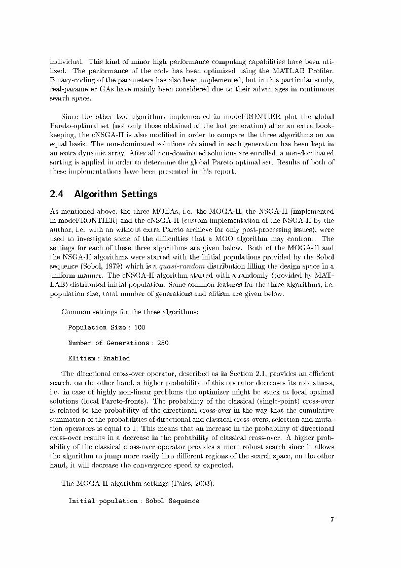
individual. This kind of minor high performance computing capabilities have been uti-lized. The performance of the code has been optimized using the MATLAB Proler.Binary-coding of the parameters has also been implemented, but in this particular study,real-parameter GAs have mainly been considered due to their advantages in continuoussearch space.

Since the other two algorithms implemented in modeFRONTIER plot the globalPareto-optimal set (not only those obtained at the last generation) after an extra book-keeping, the cNSGA-II is also modied in order to compare the three algorithms on anequal basis. The non-dominated solutions obtained in each generation has been kept inan extra dynamic array. After all non-dominated solutions are enrolled, a non-dominatedsorting is applied in order to determine the global Pareto-optimal set. Results of both ofthese implementations have been presented in this report.

2.4 Algorithm Settings

As mentioned above, the three MOEAs, i.e. the MOGA-II, the NSGA-II (implementedin modeFRONTIER) and the cNSGA-II (custom implementation of the NSGA-II by theauthor, i.e. with an without extra Pareto archieve for only post-processing issues), wereused to investigate some of the diculties that a MOO algorithm may confront. Thesettings for each of these three algorithms are given below. Both of the MOGA-II andthe NSGA-II algorithms were started with the initial populations provided by the Sobolsequence (Sobol, 1979) which is a quasi-random distribution lling the design space in auniform manner. The cNSGA-II algorithm started with a randomly (provided by MAT-LAB) distributed initial population. Some common features for the three algorithms, i.e.population size, total number of generations and elitism are given below.

Common settings for the three algorithms:

Population Size : 100

Number of Generations : 250

Elitism : Enabled

The directional cross-over operator, described as in Section 2.1, provides an ecientsearch, on the other hand, a higher probability of this operator decreases its robustness,i.e. in case of highly non-linear problems the optimizer might be stuck at local optimalsolutions (local Pareto-fronts). The probability of the classical (single-point) cross-overis related to the probability of the directional cross-over in the way that the cumulativesummation of the probabilities of directional and classical cross-overs, selection and muta-tion operators is equal to 1. This means that an increase in the probability of directionalcross-over results in a decrease in the probability of classical cross-over. A higher prob-ability of the classical cross-over operator provides a more robust search since it allowsthe algorithm to jump more easily into dierent regions of the search space, on the otherhand, it will decrease the convergence speed as expected.

The MOGA-II algorithm settings (Poles, 2003):

Initial population : Sobol Sequence

7

Prob. of Directional Cross-over : 65%

Prob. of Classical Cross-over : 20%

Prob. of Selection : 5%

Prob. of Mutation : 10%

DNA String Mutation Ration : 10%

The NSGA-II algorithm (suggested as default) settings:

Initial population : Sobol Sequence

Prob. of Cross-over : 90%

Prob. of Mutation : 10%

Distribution Index for Real-coded Cross-over : 20

Distribution Index for Real-coded Mutation : 20

The cNSGA-II algorithm settings:

Initial population : Random Distribution

Probability Distribution for the SBX, ηc : 2

Probability Distribution for the polynomial mutation, ηm : 5

8

3 Test Functions and Results

In this section, seven unconstrained MOO benchmark problems have been presented. Ineach problem, minimization of two objective functions has been considered. In the lastve well-known test cases, which were proposed by Zitzler et al. (2000), a systematicapproach has been followed to investigate a dierent aspect of diculty that a MOEAmay face. These test problems have a general structure as given in Eq. 3.1,

Minimize : f1(x),Minimize : f2(x) = g(x)h(f1(x), g(x)).

(3.1)

where f1 is a function of only x1 in each case, while the formulations of g(x) andh(f1(x), g(x)) vary together with the size of the design vector x, i.e. from 2 to 30. In allthese ve cases, the Pareto-optimal front is formed with g(x)=1.

3.1 DEB

This two-objective, two-variable minimization problem, as shown in Eq. 3.2, has beenproposed by Deb (2001) in order to illustrate the conicting scenarios between bothobjectives which result in a set of Pareto-optimal solutions. The function f1 is a functionof x1 only, thus f1 is limited by the lower and upper limits of the x1, while f2 is incontrast with the rst one, i.e. increasing f1 will result in decreasing f2 and vice versa.The Pareto-front, which corresponds to the continuous curve drawn at 0.1≤ x1 ≤1 andx2=0, is convex. The three performances are presented below in Figures 3.1 through 3.4.

Minimize : f1 (x1) = x1,

Minimize : f2 (f1, x2) =1 + x2

x1,

subject to : x1 ∈ [0.1, 1] ,x2 ∈ [0, 5] .

(3.2)

9

(a) (b)

Figure 3.1: a) All individuals obtained during the MOGA-II run for test function DEB.b) Pareto-set obtained at the end of the MOGA-II run for test function DEB.

(a) (b)

Figure 3.2: a) All individuals obtained during the NSGA-II run for test function DEB.b) Pareto-set obtained at the end of the NSGA-II run for test function DEB.

As shown in Figs. 3.1b and 3.2b, the cardinality of the Pareto-sets in applicationof both algorithms, i.e. MOGA-II and NSGA-II (in modeFRONTIER), is higher thanthe initial population size (N=100) which can be interpreted as a post-processing issue.A further book-keeping of all the non-dominated solutions in each generation which arekept in an extra array and then sorted with respect to the non-domination criterion asa nal graph. The original implementation of the NSGA-II algorithm (Deb et al., 2002)plots the Pareto-set, which corresponds to the set of non-dominated solutions at the lastgeneration, having the initial population size. In order to compare these two algorithmswith the cNSGA-II on the same basis, the results of the second version of the cNSGA-IIhave also been presented.

10

(a) (b)

Figure 3.3: a) All individuals obtained during the cNSGA-II run for test function DEB.b) Pareto-set obtained at the end of the cNSGA-II run for test function DEB.

Figure 3.4: Global Pareto set obtained using the cNSGA-II with the extra Pareto archievefor test function DEB.

3.2 POL

This second benchmark problem, which is composed of two objectives and two variables,is used by Poloni et al. (2000). It has a discontinuous, discretely spaced continuous,Pareto-optimal set which makes it dicult to know the solution beforehand.

11

Minimize : f1 (x1, x2) =[1 + (A1 −B1)

2 + (A2 −B2)2],

Minimize : f2 (x1, x2) =[(x1 + 3)2 + (x2 + 1)2

],

where A1 = 0.5 sin (1)− 2 cos (1) + sin (2)− 1.5 cos (2) ,A2 = 1.5 sin (1)− cos (1) + 2 sin (2)− 0.5 cos (2) ,B1 = 0.5 sin (x1)− 2 cos (x1) + sin (x2)− 1.5 cos (x2) ,B2 = 1.5 sin (x1)− cos (x1) + 2 sin (x2)− 0.5 cos (x2) ,

subject to : −π ≤ x1, x2 ≤ π.

(3.3)

(a) (b)

Figure 3.5: a) All individuals obtained during the MOGA-II run for test function POL.b) Pareto-set obtained at the end of the MOGA-II run for test function POL.

(a) (b)

Figure 3.6: a) All individuals obtained during the NSGA-II run for test function POL.b) Pareto-set obtained at the end of NSGA-II run for test function POL.

12

(a) (b)

Figure 3.7: a) All individuals obtained during the cNSGA-II run for test function POL.b) Pareto-set obtained at the end of the cNSGA-II run for test function POL.

Figure 3.8: Global Pareto set obtained using cNSGA-II with the extra Pareto archievefor test function POL.

3.3 ZDT1

This benchmark problem is part of Zitzler-Deb-Thiele's (ZDT) test problems on MOOcomposed of 6 cases (Zitzler et al., 2000). It has 2 objective functions and 30 designvariables, m = 30, resulting in a convex true Pareto-front having a uniform distributionof solutions accross the front. All variables lie in the range xi ∈ [0, 1]. The Pareto-optimalregion corresponds to 0≤ x1 ≤1 and xi=0 (i=2, 3, ..., m). The Pareto-optimal front isshown on the following gures 3.9 through 3.12 as the dashed line together with thesolutions obtained by the three algorithms.

13

Minimize : f1 (x1) = x1,

Minimize : f2 (f1, g) = 1−√f1

g,

where g (xi) = 1 +9

m− 1

m∑

i=2

xi,

subject to : xi ∈ [0, 1] , i = 1, 2...,m. (m = 30)

(3.4)

(a) (b)

Figure 3.9: a) All individuals obtained during the MOGA-II run for test function ZDT1.b) Pareto-set obtained at the end of the MOGA-II run for test function ZDT1.

(a) (b)

Figure 3.10: a) All individuals obtained during the NSGA-II run for test function ZDT1.b) Pareto-set obtained at the end of the NSGA-II run for test function ZDT1.

14

(a) (b)

Figure 3.11: a) All individuals obtained during the cNSGA-II run for test function ZDT1.b) Pareto-set obtained at the end of the cNSGA-II run for test function ZDT1.

Figure 3.12: Global Pareto set obtained using the cNSGA-II with the extra Paretoarchieve for test function ZDT1.

3.4 ZDT2

The ZDT2 problem has two objective functions and m=30 variables, which lie in therange xi ∈ [0, 1]. The Pareto-optimal region corresponds to 0≤ x1 ≤1 and xi=0 (i=2,3, ..., m), resulting in a non-convex true Pareto-front having a uniform distribution ofsolutions accross the front. The Pareto-optimal front for this problem is shown on thefollowing gures 3.13 through 3.16 as the dashed line together with the solutions obtainedby the three algorithms.

Minimize : f1 (x1) = x1,

Minimize : f2 (f1, g) = 1−(f1

g

)2

,

where g (xi) = 1 +9

m− 1

m∑

i=2

xi,

subject to : xi ∈ [0, 1] , i = 1, 2...,m. (m = 30)

(3.5)

15

(a) (b)

Figure 3.13: a) All individuals obtained during the MOGA-II run for test function ZDT2.b) Pareto-set obtained at the end of the MOGA-II run for test function ZDT2.

(a) (b)

Figure 3.14: a) All individuals obtained during the NSGA-II run for test function ZDT2.b) Pareto-set obtained at the end of the NSGA-II run for test function ZDT2.

16

(a) (b)

Figure 3.15: a) All individuals obtained during the cNSGA-II run for test function ZDT2.b) Pareto-set obtained at the end of the cNSGA-II run for test function ZDT2.

Figure 3.16: Global Pareto set obtained using the cNSGA-II with the extra Paretoarchieve for test function ZDT2.

3.5 ZDT3

This benchmark problem has also two objective functions and m=30 variables, whichlie in the range xi ∈ [0, 1]. In this case, the Pareto-optimal region corresponds to xi=0(i=2, 3, ..., m), but not all 0≤ x1 ≤1, resulting in a number of disconnected Pareto-frontshaving uniform distribution of solutions accross the fronts. The Pareto-optimal front forthis problem is shown on the following gures 3.13 through 3.16 as the solid black lines(red dashed lines are drawn to distinguish the discontinuous sections) together with thesolutions obtained by the three algorithms.

17

Minimize : f1 (x1) = x1,

Minimize : f2 (f1, g) = 1−√f1

g−(f1

g

)sin (10πf1) ,

where g (xi) = 1 +9

m− 1

m∑

i=2

xi,

subject to : xi ∈ [0, 1] , i = 1, 2...,m. (m = 30)

(3.6)

(a) (b)

Figure 3.17: a) All individuals obtained during the MOGA-II run for test function ZDT3.b) Pareto-set obtained at the end of the MOGA-II run for test function ZDT3.

(a) (b)

Figure 3.18: a) All individuals obtained during the NSGA-II run for test function ZDT3.b) Pareto-set obtained at the end of the NSGA-II run for test function ZDT3.

18

(a) (b)

Figure 3.19: a) All individuals obtained during the cNSGA-II run for test function ZDT3.b) Pareto-set obtained at the end of the cNSGA-II run for test function ZDT3.

Figure 3.20: Global Pareto set obtained using the cNSGA-II with the extra Paretoarchieve for test function ZDT3.

3.6 ZDT4

This benchmark problem has m=10 variables together with two objective functions. Thevariable x1 lies in the range [0,1], while others lie in [-5,5]. The Pareto-optimal frontcurve is convex. This problem has been prepared to test a MOEA in the presence ofmany local Pareto-optimal sets, further discussion can be found in Zitzler et al. (2000)and Deb (2001).

19

Minimize : f1 (x1) = x1,

Minimize : f2 (f1, g) = 1−√f1

g,

where g (xi) = 1 + 10 (m− 1) +m∑

i=2

(x2

i − 10 cos (4πxi)),

subject to : x1 ∈ [0, 1] ,xi ∈ [−5, 5] , i = 2, 3...,m. (m = 10)

(3.7)

(a) (b)

Figure 3.21: a) All individuals obtained during the MOGA-II run for test function ZDT4.b) Pareto-set obtained at the end of the MOGA-II run for test function ZDT4.

(a) (b)

Figure 3.22: a) All individuals obtained during the NSGA-II run for test function ZDT4.b) Pareto-set obtained at the end of the NSGA-II run for test function ZDT4.

20

(a) (b)

Figure 3.23: a) All individuals obtained during cNSGA-II run for test function ZDT4. b)Pareto-set obtained at the end of the cNSGA-II run for test function ZDT4.

3.7 ZDT6

This benchmark problem has also 2 objective functions and m=10 variables having anon-convex Pareto-optimal set. Actually the diculty in this problem is that the Pareto-optimal region has a non-uniform distribution of solutions and a decreasing density to-wards the Pareto-optimal front is also observed from the Figs. 3.24 through 3.27.

Minimize : f1 (x1) = 1− exp (−4x1) sin6 (6πx1) ,

Minimize : f2 (f1, g) = 1−(f1

g

)2

,

where g (xi) = 1 + 9

[m∑

i=2

xi

m− 1

]0.25

,

subject to : xi ∈ [0, 1] , i = 1, 2...,m. (m = 10)

(3.8)

21

(a) (b)

Figure 3.24: a) All individuals obtained during the MOGA-II run for test function ZDT6.b) Pareto-set obtained at the end of the MOGA-II run for test function ZDT6.

(a) (b)

Figure 3.25: a) All individuals obtained during the NSGA-II run for test function ZDT6.b) Pareto-set obtained at the end of the NSGA-II run for test function ZDT6.

22

(a) (b)

Figure 3.26: a) All individuals obtained during the cNSGA-II run for test function ZDT6.b) Pareto-set obtained at the end of the cNSGA-II run for test function ZDT6.

Figure 3.27: Global Pareto set obtained using the cNSGA-II with the extra Paretoarchieve for test function ZDT6.

23

4 Discussion of the Results and Conclusions

In this technical report, several well-known unconstrained MOO benchmark problems(Zitzler et al., 2000; Deb, 2001) have been presented in order to investigate some of thediculties that a MOEA may have to tackle. Three elitist algorithms, i.e. the MOGA-IIby Poloni and Pediroda (1997), the NSGA-II by Deb et al. (2002) (the versions imple-mented in modeFRONTIER) and the cNSGA-II (custom NSGA-II implementation bythe author in MATLAB), are employed for this purpose. Due to the availability of theexact location and dimensions of the true Pareto-optimal fronts beforehand, the perfor-mance of the algorithms (i.e. the convergence to the true Pareto front and diversity ofthe solutions along the non-dominated front) could be investigated clearly. All of thesetest cases, which were sorted in an alphabetical order, are composed of two minimizationobjectives and a number of design variables that is varying between 2 and 30.

The rst test function DEB was one of the easiest among all benchmark problemspresented. The solutions of all the three algorithms were able to converge to the truePareto-optimal front without any problem. Another aspect of the MOO problems, whichis the diversity among these non-dominated solutions, was also succesfully accomplishedby each algorithm. It is noteworthy to distinguish the convergence rate of the algo-rithms. The MOGA-II and NSGA-II (those implemented in modeFRONTIER), besideshaving a good overall convergence behavior, had also been iterating between the localPareto-optimal fronts while converging to the global one. On the other hand, from thisperspective, the cNSGA-II had shown a better performance by having fewer computationsaway from the global Pareto-optimal front. Moreover, the two algorithms (those imple-mented in modeFRONTIER), post-process the nal global Pareto-set that is composedof the non-dominated members which were archived during the generations and nallysorted with respect to domination criterion. In order to compare the performance (i.e.the number or density of the non-dominated solutions accross the Pareto-front) of thesetwo algorithms with the cNSGA-II on an equal basis, this feature was also implemented,indicated as the second version. Thus, two types of post-processing have been performedfor the cNSGA-II, i.e. rst, plotting the Pareto-set obtained at the last generation, andsecond, those saved through all generations. For the rst test problem, all the three algo-rithms (the MOGA-II, the NSGA-II and the second version of the cNSGA-II) performedsimilar in the density of the solutions viewpoint.

The second test problem (POL) presented in this report is the rst one which has adiscontinuous Pareto-front, besides ZDT3. The three performances are almost similar,but the cNSGA-II shows the same fast convergence behavior as in the rst test case. Thenext two test problems, ZDT1 and ZDT2, both have a continuous Pareto-front, but it isconvex in the former and the non-convex in the latter. In both of these problems, theMOGA-II had diculties to converge to the global Pareto-optimal front, while the othertwo algorithms performed well. The fth problem is the ZDT3, which has a discontinu-ous Pareto-front as mentioned before. The MOGA-II again had diculties in obtaininga converged set of solutions while the other two didn't have any problems. The nextproblem, the ZDT4, is one of the most dicult benchmark problems. It has a convex

24

Pareto-front and less design variables compared to ZDT1, ZDT2 and ZDT3, but the di-culty is that it has many local Pareto-optimal fronts. In this case, both the MOGA-II andthe cNSGA-II couldn't succeed to converge to the global one. The second version of thecNSGA-II hasn't been tested due to the failure observed in the rst one. The NSGA-II,which has been implemented in the modeFRONTIER outperformed the others for theZDT5. The last benchmark problem ZDT6, puts forward some diculties other thandiscontinuity or non-convexity of the Pareto front. In this case, the Pareto-optimal re-gion has a non-uniform distribution of solutions and a decreasing density towards the truePareto-front. The MOGA-II has a very good performance regarding both the convergenceand the well-spread distribution of the non-dominated solutions accross the Pareto-front.The rst version of the cNSGA-II shows a similar performance, moreover the secondversion has a continuous Pareto-curve identical to the analytical solution. The solutionsobtained by the NSGA-II (in modeFRONTIER) are not as dense and well-spread as thethose obtained by the other two algorithms.

One could argue whether there is a need for an extra post-processing step, since froma practical point of view, having a well-dened (i.e. full coverage of upper and lowerlimits of the Pareto-front) and well-distributed trade-o set which allows the user (e.g.an engineer) to have all kinds of combination of each success criterion beforehand andwithout any initial preference, is crucial enough.

As the last words, it is fair to say that the performance of the cNSGA-II is quitesatifying, especially in terms of convergence rate in problems having 2 to 10 design vari-ables. This could be explained by, rst, having a slight dierence in the application of thecross-over (SBX) and mutation operators, as explained in Section 2.3, and second, due todierences in implementation of the tournament selection operator, which promotes theconvergence as well as the diversity, in the three algorithms. At least, concerning onlythe NSGA-II algorithm and its huge popularity, it should be mentioned that there area few other versions of implemetations of this algorithm (in MATLAB) which were alsotested by the author and it is found out that the crowded tournament selection opera-tor is not implemented as originally proposed by Deb et al. (2002). Two identical pairsof solutions were able to compete in the subsequent tournaments, which stresses out themembers with lower (better) rank thus leading to loosing the diversity in the mating pool,hence in the Pareto-optimal front. The last conclusion is, that it could be mentioned thatthere is a need for an improvement of the cNSGA-II in problems which have many localPareto-optimal fronts, such as the benchmark problem ZDT4.

25

Bibliography

Corne, D., Knowles, J., and Oates, M. (2000). The pareto envelope-based selectionalgorithm for multiobjective optimization. pages 839848. 6th International Conferenceon Parallel Problem Solving from Nature.

Deb, K. (1999). Multi-objective genetic algorithms: Problem diculties and constructionof test problems. Evolutionary Computation, 7:205230.

Deb, K. (2001). Multi-Objective Optimization using Evolutionary Algorithms. John Wileyand Sons, Ltd.

Deb, K. (2006). Optimization for Engineering Design. Prentice-Hall of India Pvt. Ltd.

Deb, K. and Agrawal, R. (1995). Simulated binary crossover for continuous search space.Complex Systems, 9:115148.

Deb, K., Agrawal, S., Pratap, A., and Meyerivan, T. (2002). A fast and elitist multi-objective genetic algorithm: NSGA-II. IEEE Transactions on Evolutionary Compu-

tation, 6:182197.

Deb, K. and Kumar, A. (1995). Real-coded genetic algorithms with simulated binarycrossover: Studies on multi-modal and multi-objective problems. Complex Systems,9:431454.

Deb, K., Mohan, M., and Mishra, S. (2003). Towards a quick computation of well-spreadpareto-optimal solutions. volume 2632 of Lecture Notes in Computer Science, pages222236. Springer Berlin - Heidelberg.

ESTECO s.r.l. (2007). http://www.esteco.com. (version v4.0).

Fonseca, C. and Fleming, P. (1993). Genetic algorithms for multiobjective optimization:Formulation, discussion and generalization. 5th International Conference on GeneticAlgorithms, USA.

Goldberg, D. (1989). Genetic Algorithms in Search, Optimization & Machine Learning.Addison Wesley Longman, Inc.

Horn, J., Nafpliotis, N., and Goldberg, D. (1994). A niched pareto genetic algorithmfor multiobjective optimization. pages 8287. First IEEE Conference on EvolutionaryComputation. IEEE World Congress on Computational Intelligence.

Knowles, J. and Corne, D. (1998). The pareto archived evolution strategy: A new baselinealgorithm for pareto multiobjective optimization. pages 250259. Parallel ProblemSolving from Nature - PPSN V. 5th International Conference.

Parks, G. and Miller, I. (1998). Selective breeding in a multiobjective genetic algorithm.pages 250259. Parallel Problem Solving from Nature - PPSN V. 5th InternationalConference.

26

Poles, S. (2003). MOGA-II, an improved multi-objective genetic algorithm. TechnicalReport 006, ESTECO s.r.l.

Poles, S., Geremia, P., Campos, F., Weston, S., and Islam, M. (2007). MOGA-II for anautomotive cooling duct optimization on distributed resources. volume 4403 of LectureNotes in Computer Science, pages 633644. Springer Berlin - Heidelberg.

Poles, S., Rigoni, E., and Robi£, T. (2004). MOGA-II performance on noisy optimizationproblems. Bioinspired Optimization Methods and their Applications (BIOMA).

Poloni, C., Giurgevich, A., Onesti, L., and Pediroda, V. (2000). Hybridization of a mul-tiobjective genetic algorithm, a neural network and a classical optimizer for a complexdesign problem in uid dynamics. Computer Methods in Applied Mechanics and Engi-

neering, 186:403420.

Poloni, C. and Pediroda, V. (1997). GA coupled with computationally expensive simula-

tions: tools to improve eciency, chapter Genetic Algorithms and Evolution Strategiesin Engineering and Computer Science, pages 267288. John Wiley and Sons.

Rigoni, E. and Poles, S. (2005). NBI and MOGA-II, two complementary algorithmsfor multi-objective optimizations. In Branke, J., Deb, K., Miettinen, K., and Steuer,R. E., editors, Practical Approaches to Multi-Objective Optimization, number 04461 inDagstuhl Seminar Proceedings, Dagstuhl, Germany. Internationales Begegnungs- undForschungszentrum für Informatik (IBFI), Schloss Dagstuhl, Germany.

Schaer, J. D. (1985). Multiple objective optimization with vector evaluated geneticalgorithms. In Proceedings of the 1st International Conference on Genetic Algorithms,pages 93100, Hillsdale, NJ, USA. L. Erlbaum Associates Inc.

Sobol, I. (1979). On the systematic search in a hypercube. SIAM Journal on Numerical

Analysis, 16:790793.

Srinivas, N. and Deb, K. (1994). Multi-objective optimization using non-dominated sort-ing in genetic algorithms. Evolutionary Computation, 2:221248.

Yamamoto, K. and Inoue, O. (1995). New evolutionary direction operator for geneticalgorithms. AIAA Journal, 33:19901993.

Zitzler, E., Deb, K., and Thiele, L. (2000). Comparison of multiobjective evolutionaryalgorithms: Emprical results. Evolutionary Computation, 8:173195.

Zitzler, E., Laumanns, M., and Thiele, L. (2001). Spea2: Improving the strength paretoevolutionary algorithm. Technical Report 103, Swiss Federal Institute of Technology(ETH) Zurich.

Zitzler, E. and Thiele, L. (1998). An evolutionary algorithm for multiobjective optimiza-tion: the strength pareto approach. Technical Report 43, Swiss Federal Institute ofTechnology (ETH) Zurich.

Zitzler, E. and Thiele, L. (1999). Multiobjective evolutionary algorithms: a comparativecase study and the strength pareto approach. IEEE Transactions on Evolutionary

Computation, 3:257271.

27

F TECHNICAL REPORT-II

C. C. Tutum and J. H. Hattel, "A benchmark study for constrained multi-objective prob-

lems", October 2009.

193

Technical Report-2

A Benchmark Study for Constrained

Multi-objective Optimization Problems

Cem Celal Tutum

Jesper Henri Hattel

Process Modelling Group

Department of Mechanical Engineering

Technical University of Denmark

Produktionstorvet, Kgs. Lyngby

2800, Denmark

October 1st, 2009

Table of Contents

1 Introduction 1

2 A Brief Description of the Algorithms 2

2.1 Multi-objective Genetic Algorithm (MOGA-II) . . . . . . . . . . . . . . . 2

2.2 Non-dominated Sorting Genetic Algorithm (NSGA-II) . . . . . . . . . . . 4

2.3 Custom implementation of the NSGA-II (cNSGA-II) . . . . . . . . . . . . 5

2.4 Algorithm Settings . . . . . . . . . . . . . . . . . . . . . . . . . . . . . . . 6

3 Test Functions and Results 9

3.1 BNH . . . . . . . . . . . . . . . . . . . . . . . . . . . . . . . . . . . . . . . 9

3.2 DEB (CONSTR) . . . . . . . . . . . . . . . . . . . . . . . . . . . . . . . . 12

3.3 OSY . . . . . . . . . . . . . . . . . . . . . . . . . . . . . . . . . . . . . . . 14

3.4 SRN . . . . . . . . . . . . . . . . . . . . . . . . . . . . . . . . . . . . . . . 17

3.5 TNK . . . . . . . . . . . . . . . . . . . . . . . . . . . . . . . . . . . . . . . 18

4 Discussion of the Results and Conclusions 21

Bibliography 23

iii

1 Introduction

One of the goals of an ideal multi-objective optimization (MOO) procedure, in which the

objectives are conicting with each other and there is no higher level information (user

preferences) beforehand that is leading to a biased search, is to nd as many Pareto-

optimal solutions as possible. Due to the population based search strategy of an evo-

lutionary algorithm (EA), it is possible to obtain a set of Pareto-optimal solutions in a

single simulation run. Besides aiming for a converged solution set as in a single objective

optimization (SOO) case, it is also an important task for a multi-objective evolutionary

algorithm (MOEA) to have well-distribution or diversity among these trade-o solutions,

which is specic to MOO. Some of the problem features that may cause a multi-objective

GA diculty have been systematically investigated and procedures of constructing multi-

objective test problems addressing dierent aspects of diculties are presented before by

Deb (1999b). The convergence to the global Pareto-front (among local ones) as well as

satisfying the well-distribution of these non-dominated solutions in a complex (convex or

non-convex as well as continuous or discontinuous) objective space can be highlighted as

major criteria. Moreover, the presence of constraints, whether they are equality (hard)

or inequality, in an MOO problem would make the problems even more severe. Thus the

challange of obtaining the two major success criteria from an MOEA (i.e. the conver-

gence and the diversity), can be accomplished only by using a proper constraint handling

strategy.

This technical report presents several well-known constrained MOO benchmark prob-

lems in order to investigate some of the diculties as mentioned above that a MOEA

may have to tackle. Three elitist algorithms, i.e. the MOGA-II by Poloni and Pediroda

(1997), the NSGA-II by Deb et al. (2002) (the versions implemented in modeFRON-

TIER) and the cNSGA-II (custom NSGA-II implementation by the author in MATLAB

with two versions, see the details in Section 2.3), are employed for this purpose. Two

types of constraint handling strategies, i.e. the Penalty Function Approach and the Con-

strained Tournament Method, had also been tested alongside. The MOGA-II uses the

former approach, while the NSGA-II and the cNSGA-II use the latter approach. Besides

a clear distinction of the dierent convergence and the diversity behavior of these three

algorithms reported, it is also interesting to distinguish the convergence speeds.

1

2 A Brief Description of the Algorithms

In this section, a brief description of the three elitist algorithms, i.e. the MOGA-II by

Poloni and Pediroda (1997), the NSGA-II by Deb et al. (2002) (the versions implemented

in modeFRONTIER) and the cNSGA-II (the custom NSGA-II implementation by the

author in MATLAB), are presented toether with two dierent constraint handling strate-

gies, i.e. the penalty function approach in the MOGA-II and the constrained tournament

selection in the NSGA-II and the cNSGA-II.

2.1 Multi-objective Genetic Algorithm (MOGA-II)

MOGA-II is one of the new elitist evolutionary algorithms designed for MOO problems

that is implemented in the commercial MOO software modeFRONTIER (ESTECO s.r.l.,

2007). It is an improved version of the MOGA by Poloni and Pediroda (1997), but it

should not be confused with the non-elitist MOGA developed by Fonseca and Fleming

(1993).

As in classical genetic algorithms (Goldberg, 1989), the internal encoding in MOGA-

II is based on binary coding that each design variable is represented as a binary string,

i.e. 0100, 1101101, etc., where the length of the string depends on the number of allowed

values for the variable. MOGA-II starts with the initial binary-coded population P of

size N and an empty elite set E = ∅. P ′ = P ∪ E is computed every generation. If the

population size of P ′ is greater than the population size of P , the exceeding members inP ′ are randomly removed in order to reduce the population size to the initial size. Fol-

lowing this step, the evolution takes place in which P ′ is updated to P ′′ by applying all

MOGA operators, i.e. classical cross-over, directional cross-over, mutation and selection.

The classical (single-point) cross-over is a well-known genetic algorithm operator in

which two parents (individuals from the mating pool) are randomly chosen and some por-

tions of these binary strings are exchanged between each other. In single-point cross-over,

the crossing site is randomly chosen and all bits on the right side of the crossing site are

swapped as shown schematically in Fig. 2.1. In MOGA-II, single point cross-over starts

by taking the current individual-i as the rst parent. The second parent (individual-j)is chosen by means of a multi-objective tournament selection on a randomly selected

population subset (Poles et al., 2007, 2004; Rigoni and Poles, 2005). After the cross-over

operation is performed, one of the resulting strings (children) is randomly selected to be

the new individual.

The directional cross-over assumes that a direction of improvement, which remindsthe search direction in classical algorithms that is relatively more expensive to compute,

can be detected by comparing the tness values of two reference individuals selected from

the same generation similar to the idea presented by Yamamoto and Inoue (1995). The

selection of these two reference individuals (parents) can be done using any available se-

lection scheme. In MOGA-II, potential candidates are met in a random walk of assigned

2

Figure 2.1: Schematic procedure of single-point crossover.

number of steps for each individual and then the two of them with the best tnesses are

chosen. The new individual is then created by moving in a randomly weighted direction

that lies within the ones originated by the starting point (current individual) and two

other parents selected by the local tournament, as shown in Fig. 2.2.

Figure 2.2: Schematic procedure of directional crossover in MOGA-II (Poles et al., 2004,

2007; Rigoni and Poles, 2005).

The mutation operator is responsible for perturbing the binary string, i.e. changing

1 to 0 or vice versa, with a given DNA String Mutation Ratio (probability). The mu-tation operator can be said to be responsible of the local search as well as maintaining

the diversity in the population (Deb, 2006).

Figure 2.3: Schematic procedure of mutation for a given DNA string mutation ratio,

pm=30%.

The tness of the population P ′′ is calculated. Non-domination sorting is performed

and all non-dominated designs of P ′′ are copied to the elite set, E which is then updated

by removing duplicated or dominated designs. Next, E is resized if it is larger than the

population size N removing randomly the exceeding points. Finally, the rst generation

is created and P ′′ is assigned as the new initial population P for the next generation.

This iterative loop continues until the stopping criterion is met, i.e. the user-dened

total number of generations (Poles, 2003).

3

2.2 Non-dominated Sorting Genetic Algorithm (NSGA-II)

NSGA-II is a multi-objective evolutionary algorithm (MOEA) proposed by Deb et al.

(2002), which enables nding well-spread multiple Pareto-optimal solutions for an MOO

problem by incorporating three substantial features, i.e., elitism, non-dominated sort-

ing, and a diversity preserving mechanism. Elitism, which is a genetic operator used to

preserve the good solutions through the generations, is also shown to increase the con-

vergence speed of an MOEA Zitzler et al. (2000).

Figure 2.4: The crowding distance calculation (adapted from Deb et al. (2002)).

The preservation of well-distributed (diverse) nondominated solutions is maintained

by the crowding distance operator. The crowding distance, which is calculated frontwise,

is a measure of how close an individual is to its neighbors. In order to get an estimate of

the density of solutions surrounding a particular solution in the population, the average

distance between two points on either side of the solution along each of the objectives is

calculated. This quantity di serves as an estimate of the perimeter of the cuboid formed

by using the nearest neighbors as the vertices. A schematic view of the procedure for

the computation of the crowding distance for an ith individual is shown in Fig. 2.4, and

formulated as (Deb et al., 2002),

dImi

= dImi

+f

(Imi+1)

m − f (Imi−1)

m

fmaxm − fmin

m

, for i = 2, ..., l − 1 (2.1)

where I(i) is the solution index of the ith member in the (worse order) sorted list, mis the number of objectives and l is the number of the individuals in that particular front.The rst and the last individuals are assigned an innite distance in order to emphasize

their tness, hence preserving them for the next generation. A large average crowding

distance will result in a better diversity in the population.

The schematic view of NSGA-II on a owchart is shown in 2.5. The procedure starts

with an initialization of the parent population, P0, followed by sorting (ranking) the

members of the population based on nondomination into each front, Fi. Each individual

is assigned two tness values, i.e. the one related to its nondomination level (front or

rank, i.e. Fi refers to front with rank i in Fig. 2.4) and the crowding distance. Parents areselected by using binary (crowded) tournament selection based on these two measures.

4

Figure 2.5: Schematic view of the NSGA-II procedure (Deb et al., 2002).

An individual is selected if its rank is less than the other, since the minimization is

assumed, or if the crowding distance is greater than the other. The selected population

generates o-springs, Qt, by the application of usual genetic operators, i.e. crossover and

mutation (simulated binary crossover (SBX), (Deb and Agrawal, 1995; Deb and Kumar,

1995) and polynomial mutation for real parameter GA in this case) (Deb, 2001; Goldberg,

1989). Since all the parent and the ospring individuals are included in the combined

population, Rt, elitism is ensured. In order to reduce the size of the population of the

next generation from 2N to N , nondomination sorting is applied and the individuals with

relatively lowest possible ranks are accomodated until the size of the population exceeds

N . Then the individuals in front Fi are selected based on their crowding distance. This

cycle is repeated until the stopping criterion, i.e. the total number of generations, is met.

For further details, please consult the original study (Deb et al., 2002).

2.3 Custom implementation of the NSGA-II (cNSGA-II)

This custom (personal) implementation of the NSGA-II (cNSGA-II) by the author should

not be confused with the clustered NSGA-II (C-NSGA-II) (Deb et al., 2003) which uses

an identical clustering technique to that used in the SPEA (Zitzler and Thiele, 1998,

1999) in order to obtain a well-spread distribution.

The cNSGA-II has a minor change compared to the original NSGA-II in the applica-

tion of the SBX and polynomial mutation operators. Instead of applying these operators

with predened probabilities for each, a xed percentage of the population (90%) has

been randomly selected as the set of parents in order to produce the children with a

predened distribution index (ηc). Following this, polynomial mutation is applied on the

rest of the population (10%), which didn't participate in the SBX operation. By doing

this, it is ensured that all members will participate in these operations. The percentage

of the population on which the SBX operator is applied is chosen higher compared to the

one for the polynomial mutation (i.e. 90% vs. 10%) in order to enforce the search on a

larger portion of the search region, in addition to the application of a relatively smaller

distribution index (resulting in a wider spread with respect to the parents, aiming at a

uniform distribution in the search space). The polynomial mutation operator is applied

5

with a relatively higher distribution index in order to make a ner search (producing the

children closer to the parents).

The computation of the tness values are vectorized instead of looping over each

individual. This kind of minor high performance computing capabilities have been uti-

lized. The performance of the code has been optimized using the MATLAB Proler.

Binary-coding of the parameters has also been implemented, but in this particular study,

real-parameter GAs have mainly been considered due to their advantages in continuous

search space.

Since the other two algorithms implemented in modeFRONTIER plot the global

Pareto-optimal set (not only those obtained at the last generation) after an extra book-

keeping, the cNSGA-II is also modied in order to compare the three algorithms on an

equal basis. The non-dominated solutions obtained in each generation has been kept in

an extra dynamic array. After all non-dominated solutions are enrolled, a non-dominated

sorting is applied in order to determine the global Pareto-optimal set. Results of both of

these implementations have been presented in this report.

2.4 Algorithm Settings

As mentioned above, the three MOEAs, i.e. the MOGA-II, the NSGA-II (implemented

in modeFRONTIER) and the cNSGA-II (custom implementation of the NSGA-II by the

author, i.e. with an without extra Pareto archieve for only post-processing issues), were

used to investigate some of the diculties that a MOO algorithm may confront. The

settings for each of these three algorithms are given below. Both of the MOGA-II and

the NSGA-II algorithms were started with the initial populations provided by the Sobol

sequence (Sobol, 1979) which is a quasi-random distribution lling the design space in a

uniform manner. The cNSGA-II algorithm started with a randomly (provided by MAT-

LAB) distributed initial population. Some common features for the three algorithms, i.e.

population size, total number of generations and elitism are given below.

Common settings for the three algorithms:

Population Size : 100

Number of Generations : 250

Elitism : Enabled

The directional cross-over operator, described as in Section 2.1, provides an ecient

search, on the other hand, a higher probability of this operator decreases its robustness,

i.e. in case of highly non-linear problems the optimizer might be stuck at local optimal

solutions (local Pareto-fronts). The probability of the classical (single-point) cross-over

is related to the probability of the directional cross-over in the way that the cumulative

summation of the probabilities of directional and classical cross-overs, selection and muta-

tion operators is equal to 1. This means that an increase in the probability of directional

cross-over results in a decrease in the probability of classical cross-over. A higher prob-

ability of the classical cross-over operator provides a more robust search since it allows

the algorithm to jump more easily into dierent regions of the search space, on the other

6

hand, it will decrease the convergence speed as expected.

The constraint handling strategy in the MOGA-II depends on the penalization of the

objectives which is a very popular one (due to its easy and relatively eective imple-

mentation) among others, e.g. ignoring infeasible solutions, Jiménez-Verdegay-Goméz-

Skarmeta's method, Ray-Tai-Seow's Method, for further details see Deb (2001). For a

given multi-objective minimization problem (a maximization problem can also be con-

verted into a minimization problem by the duality principle, i.e. the objective function is

multiplied by -1) having inequality constraints (which are normalized to have the same

order) of type gj(xi) ≥ 0 (for j=1,2, ..., nineq), rst, all constraint violations (wj) are

computed for each individual xi, then summed up to give the overall constraint violation

Ω(xi) as follows,

wj(xi) =

|gj(xi)|, if gj(xi) < 0,0 otherwise.

⇒ Ω(xi) =nineq∑

j=1

wj(xi) (2.2)

next, this overall constraint violation (Ω(xi)) is multiplied with a penalty parameter

Rm (the subscript-m is the number of the objectives, hence Rm is a vector of penalty

terms), and then the product is added to each of the objective function values.

Fm(xi) = fm(xi) +RmΩ(xi) (2.3)

Here Fm(xi) denotes the modied objective functions which take the constraints into

account via a penalty parameter. The overall constraint violation will be zero for a fea-

sible solution, which means that Fm will be equal to the original objective function fm.

Obviously, an infeasible solution will have a modied objective function greater than the

original one (Fm > fm) due to the addition of the penalty term. For a problem of the

minimization of the objectives, an MOEA will rst assign rank on each solution based on

its modied objective, by this way, it will try to promote the solutions which have lower

tness (objective) values, in other words, since the feasible solutions will dominate the

infeasible ones, an MOEA will enhance the probability of survival of the feasible solu-

tions. Further details about the application of the penalty function approach are given in

the literature, e.g. Deb (1999a) (for MOO problems) and Michalewicz (1992) (for SOO

problems). However, this approach is not accurate enough, since ranking depends on

the chosen penalty parameter and as a result, infeasible solutions which are close to the

constraint boundary can occupy the same front with feasible solutions.

The MOGA-II algorithm settings (Poles, 2003):

Initial population : Sobol Sequence

Prob. of Directional Cross-over : 65%

Prob. of Classical Cross-over : 20%

Prob. of Selection : 5%

Prob. of Mutation : 10%

DNA String Mutation Ration : 10%

7

Constraint Handling Algorithm : Penalty Function Method

The NSGA-II uses the Constrained Tournament Method, developed by K. Deb, which

incorporates a denition or condition of constrain-domination (modied version of the

usual denition of domination in the presence of constraints) for the Binary Tournament

Selection (BTS) operator, which does not need any penalty parameter. Each solution

can be either feasible or infeasible in a constrained problem. The BTS operator needs to

compare two solutions in order to select the better one, hence it needs deal with three

conditions: i) both solutions can be feasible, ii) one of them can be feasible, and the other

one can be infeasible, or iii) both solutions can be infeasible. It is obvious to decide for

the second case (ii), a feasible solution is preferred. In the last case, the infeasible solutionwith the lower constraint violation is chosen. In the rst case, which is not obvious as in

other cases, the solutions will be compared with respect to their non-domination levels

(ranks) and if they belong to the same front, the crowding distance sorting operator will

resolve the tie by selecting the solution located in a less crowded region. This approach

will classify the infeasible solutions more precisely compared to the penalty approach (al-

most each infeasible solution will belong to a dierent front unless they have an identical

constraint violation), while having a similar front distribution in the feasible region.

The NSGA-II algorithm (suggested as default) settings:

Initial population : Sobol Sequence

Prob. of Cross-over : 90%

Prob. of Mutation : 10%

Distribution Index for Real-coded Cross-over : 20

Distribution Index for Real-coded Mutation : 20

Constraint Handling Algorithm : Constrained Tournament Method

The cNSGA-II algorithm settings:

Initial population : Random Distribution

Probability Distribution for the SBX, ηc : 2

Probability Distribution for the polynomial mutation, ηm : 5

Constraint Handling Algorithm : Constrained Tournament Method

8

3 Test Functions and Results

In this section, ve well-known constrained MOO benchmark problems, i.e. BNH, DEB,

OSY, SRN and TNK, have been presented in an alphabetical order. In each problem,

the minimization of two objective functions, having 2 to 6 design variables, has been

considered. The convergence and the diversity performances of the three algorithms,

the MOGA-II and the NSGA-II (implemented in the modeFRONTIER) as well as the

cNSGA-II (the custom NSGA-II implementation by the author in MATLAB), have been

compared.

3.1 BNH

This benchmark case is a two-objective (f1 and f2 to be minimized), two-variable (x1

and x2) optimization problem with two nonlinear constraints presented by Binh and

Korn (1997) for testing the performance of their Multi-Objective Evolution Strategy

(MOBES) on nonlinear constraints. The results obtained by the three algorithms (the

MOGA-II, the NSGA-II and the cNSGA-II) are presented below. First graph on a row

presents all the solutions obtained through all generations. The feasible and unfeasible

solutions are denoted by blue and red markers, respectively. In the second graph on the

same corresponding raw, Pareto solutions are drawn. As mentioned before, the MOGA-II

and the NSGA-II (which are implemented in the modeFRONTIER) post-process all the

Pareto-optimal solutions obtained along generations. Three graphs of the cNSGA-II for

each problem are shown following the results of the rst two aforementioned algorithms.

The last two of these three results in each problem present the Pareto-optimal solutions

obtained by the cNSGA-II. The second graph of the Pareto-front is obtained with an

identical post-processing step as in the MOGA-II and the NSGA-II. This presentation

scheme is followed for each benchmark problem.

Minimize : f1(x) = 4x21 + 4x2

2,

Minimize : f2(x) = (x1 − 5)2 + (x2 − 5)2,

subject to : g1(x) = (x1 − 5)2 + x22 ≤ 25,

g2(x) = (x1 − 8)2 + (x2 + 3)2 ≥ 7.7,0 ≤ x1 ≤ 5,0 ≤ x2 ≤ 3.

(3.1)

9

(a) (b)

Figure 3.1: a) All individuals obtained during the MOGA-II run for the test function

BNH. b) The Pareto-set obtained at the end of the MOGA-II run for the test function

BNH.

(a) (b)

Figure 3.2: a) All individuals obtained during the NSGA-II run for the test function

BNH. b) The Pareto-set obtained at the end of NSGA-II run for the test function BNH.

10

(a) (b)

Figure 3.3: a) All individuals obtained during the cNSGA-II run for the test function

BNH. b) The Pareto-set obtained at the end of the cNSGA-II run for the test function

BNH.

Figure 3.4: The global Pareto set obtained using the cNSGA-II with Pareto archieve

strategy for the test function BNH.

11

3.2 DEB (CONSTR)

The test function DEB (CONSTR) is used in Deb et al. (2002) and discussed thoroughly

in Deb (2001). The rst objective function f1 depends only on x1, the second objective

function has two variables.

Minimize : f1(x) = x1,

Minimize : f2(x) =1 + x2

x1,

subject to : g1(x) = x2 + 9x1 ≥ 6,g2(x) = −x2 + 9x1 ≥ 1,0.1 ≤ x1 ≤ 1,0 ≤ x2 ≤ 5.

(3.2)

(a) (b)

Figure 3.5: a) All individuals obtained during the MOGA-II run for the test function

DEB. b) The Pareto-set obtained at the end of the MOGA-II run for the test function

DEB.

12

(a) (b)

Figure 3.6: a) All individuals obtained during the NSGA-II run for the test function

DEB. b) The Pareto-set obtained at the end of the NSGA-II run for the test function

DEB.

(a) (b)

Figure 3.7: a) All individuals obtained during the cNSGA-II run for the test function

DEB. b) The Pareto-set obtained at the end of the cNSGA-II run for the test function

DEB.

Figure 3.8: The global Pareto set obtained using the cNSGA-II with the Pareto archieve

strategy for the test function DEB.

13

3.3 OSY

This benchmark problem, which is used by Osyczka and Kundu (1995), contains two

nonlinear objective functions and six constraints (four of them are linear). This test case

is the most dicult test case among ve benchmark problems, since the Pareto-optimal

front is composed of ve regions and each region demands an MOEA to maintain its

subpopulations at dierent intersections of constraint boundaries (Deb, 2001).

Minimize : f1(x) = −[25(x1 − 2)2 + (x2 − 2)2 + (x3 − 1)2 + (x4 − 4)2 + (x5 − 1)2],

Minimize : f2(x) = x21 + x2

2 + x23 + x2

4 + x25 + x2

6,

subject to : g1(x) = x1 + x2 − 2 ≥ 0,g2(x) = 6− x1 − x2 ≥ 0,g3(x) = 2− x2 + x1 ≥ 0,g4(x) = 2− x1 + 3x2 ≥ 1,

g5(x) = 4− (x3 − 3)2 − x4 ≥ 0,

g6(x) = (x5 − 3)2 + x6 − 4 ≥ 0,0 ≤ x1, x2, x6 ≤ 10,1 ≤ x3, x5 ≤ 5,0 ≤ x4 ≤ 6.

(3.3)

(a) (b)

Figure 3.9: a) All individuals obtained during the MOGA-II run for the test function

OSY. b) The Pareto-set obtained at the end of the MOGA-II run for the test function

OSY.

14

(a) (b)

Figure 3.10: a) All individuals obtained during the NSGA-II run for the test function

OSY. b) The Pareto-set obtained at the end of the NSGA-II run for the test function

OSY.

(a) (b)

Figure 3.11: a) All individuals obtained during the cNSGA-II run for the test function

OSY. b) The Pareto-set obtained at the end of the cNSGA-II run for the test function

OSY.

15

Figure 3.12: The global Pareto set obtained using the cNSGA-II with the Pareto archieve

strategy for the test function OSY.

16

3.4 SRN

The test problem presented here is used by Srinivas and Deb (1994).

Minimize : f1(x) = 2 + (x1 − 2)2 + (x2 − 1)2 ,

Minimize : f2(x) = 9x1 − (x2 − 1)2 ,

subject to : g1(x) = x21 + x2

2 ≤ 225,g2(x) = x1 − 3x2 + 10 ≤ 0,− 20 ≤ x1 ≤ 20,− 20 ≤ x2 ≤ 20.

(3.4)

(a) (b)

Figure 3.13: a) All individuals obtained during the MOGA-II run for the test function

SRN. (b)The Pareto-set obtained at the end of the MOGA-II run for the test function

SRN.

(a) (b)

Figure 3.14: a) All individuals obtained during the NSGA-II run for the test function

SRN. b) The Pareto-set obtained at the end of the NSGA-II run for the test function

SRN.

17

(a) (b)

Figure 3.15: a) All individuals obtained during the cNSGA-II run for the test function

SRN. b) The Pareto-set obtained at the end of the cNSGA-II run for the test function

SRN.

Figure 3.16: The global Pareto set obtained using the cNSGA-II with the Pareto archieve

strategy for the test function SRN.

3.5 TNK

Tanaka (1995) used the following two-variable problem of which the solution, i.e. the

Pareto-optimal front, is discontinuous.

Minimize : f1(x) = x1,

Minimize : f2(x) = x2,

subject to : g1(x) = x21 + x2

2 − 1− 0.1 cos(

16 arctan(x1

x2

))≥ 0,

g2(x) = (x1 − 0.5)2 + (x2 − 0.5)2 ≤ 0.5,0 ≤ x1 ≤ π,0 ≤ x2 ≤ π.

(3.5)

18

(a) (b)

Figure 3.17: a) All individuals obtained during the MOGA-II run for the test function

TNK. b) The Pareto-set obtained at the end of the MOGA-II run for the test function

TNK.

(a) (b)

Figure 3.18: a) All individuals obtained during the NSGA-II run for the test function

TNK. b) The Pareto-set obtained at the end of the NSGA-II run for the test function

TNK.

19

(a) (b)

Figure 3.19: a) All individuals obtained during the cNSGA-II run for the test function

TNK. b) The Pareto-set obtained at the end of the cNSGA-II run for the test function

TNK.

Figure 3.20: The global Pareto set obtained using the cNSGA-II with the Pareto archieve

strategy for the test function TNK.

20

4 Discussion of the Results and Conclusions

In this technical report, ve well-known constrained MOO benchmark problems, i.e.

BNH, DEB (CONSTR), OSY, SRN and TNK, have been presented. Some of the dif-

culties that an MOEA may have to tackle have been investigated by using three elitist

algorithms, the MOGA-II and the NSGA-II implemented in the modeFRONTIER and

the cNSGA-II implemented by the author in MATLAB. Two types of constraint han-

dling strategies, i.e. the Penalty Function Approach and the Constrained Tournament

Method, have also been tested alongside. The MOGA-II uses the former approach, while

the NSGA-II and the cNSGA-II use the latter approach. All of the test problems, which

are sorted in an alphabetical order (i.e. not according to diculty level), are composed

of two minimization of objectives and a number of design variables varying from 2 to 6.

Moreover, both linear and non-linear inequality constraints are used varying between 2

and 6, excluding the bounds on the variables.

In the rst test function BNH, the solutions of all the three algorithms were able to

converge to the true Pareto-optimal front without any problem and the diversity among

the non-dominated solutions was also succesfully obtained by each algorithm. It is note-

worthy to distinguish the convergence rate of the algorithms. The MOGA-II has spent

less time (i.e. less number of computations) near the Pareto front compared to the NSGA-

II, but on the other hand the NSGA-II has fully covered the true Pareto-front while the

density of the solutions obtained by the MOGA-II has been decreasing towards the right

boundary of the front. The cNSGA-II clearly outperformed these two algorithms by con-

verging much faster and spending less computations near the Pareto front. In the second

test problem DEB (CONSTR), although the NSGA-II was more succesful in nding a

larger amount of non-dominated solutions compared to the MOGA-II, the number of un-

feasible solutions was also much higher which is not preferable. On the other hand, the

MOGA-II was not able to cover the left arm of the Pareto-front. The performance of the

cNSGA-II was again satisfying compared to the others in the sense that it both converged

faster and found a larger amount of non-dominated solutions which were distributed ac-

cross the Pareto-front in a very uniform way. The third test problem OSY is the most

dicult one of all ve benchmark cases, since the Pareto-optimal front consists of ve

regions and each region demands an MOEA to maintain its subpopulations at dierent

intersections of constraint boundaries. As seen from the results, the MOGA-II was clearly

unsuccessful in this problem since it could only nd the middle (the third) distinct part of

the Pareto-front. The NSGA-II was able to capture almost all ve regions of the Pareto-

front, but the density in the lower region is quite low. The cNSGA-II performed well

considering both having converged and well-spread distributed non-dominated solutions,

although it spent more computations outside the Pareto-front compared to the previous

test cases. In the next test problem SRN, the convergence behavior of the two algorithms,

the MOGA-II and the NSGA-II, was similar. A nice (uniform and dence) distribution

of the non-dominated solutions accross the Pareto-front is seen clearly. The convergence

rate of the cNSGA-II was again similar to the previous cases, i.e. fast convergence with

less computations outside the Pareto-front. In the last benchmark case TNK, which has

a discontinuous Pareto-optimal front, the performance of the cNSGA-II was dominating

21

the other two algorithms.

These results show the performance of both dierent MOEAs and the two dierent

constraint handling strategies, i.e. the penalty function approach and the constrained

tournament method. Although the NSGA-II and the cNSGA-II uses the same constraint

handling strategies (constrained tournament method), they show very dierent conver-

gence characteristics. The NSGA-II is claimed to be implemented as in the original study

by Deb (2001), but at least for the constrained problems presented here, it is fair to say

that it is not as succesfull as the original one. On the other hand, the success of the

cNSGA-II could be explained by a slightly dierent strategy in applying the SBX oper-

ator, i.e. ensuring all members to be updated with a chosen low probability distribution

number (ηc=2), hence obtaining a large diversity in the begining of the evolution, then to-

wards the end, narrowing the search which helps convergence. Moreover, the constrained

tournament operator (proposed by K. Deb), which incorporates the constrain-domination

denition, helps the cNSGA-II to converge to the true Pareto-front in a substantially quick

way, besides supplying a very uniform distribution. Finally, it can be concluded that the

performance of the cNSGA-II is satisfying especially regarding the convergence rate for

the constrained problems presented here (with up to 6 design variables). It is planned to

apply it on real-world (e.g. engineering) applications. An evolutionary hybrid algorithm,

which uses the cNSGA-II as a robust search technique together with a local search algo-

rithm, e.g. the Sequential Quadratic Programming (SQP), which improves the accuracy

and the number of function evaluations, is under preparation.

22

Bibliography

Binh, T. and U. Korn (1997). Mobes: A multi-objective evolution strategy for constrained

optimization problems. pp. 176182. The Third International Conference on Genetic

Algorithms (Mendel 97).

Deb, K. (1999a). Evolutionary algorithms for multi-criterion optimization in engineering

design, pp. 135161. Evolutionary Algorithms in Engineering and Computer Science.

Chichester, UK: John Wiley and Sons.

Deb, K. (1999b). Multi-objective genetic algorithms: Problem diculties and construc-

tion of test problems. Evolutionary Computation 7, 205230.

Deb, K. (2001). Multi-Objective Optimization using Evolutionary Algorithms. John Wiley

and Sons, Ltd.

Deb, K. (2006). Optimization for Engineering Design. Prentice-Hall of India Pvt. Ltd.

Deb, K. and R. Agrawal (1995). Simulated binary crossover for continuous search space.

Complex Systems 9, 115148.

Deb, K., S. Agrawal, A. Pratap, and T. Meyerivan (2002). A fast and elitist multi-

objective genetic algorithm: NSGA-II. IEEE Transactions on Evolutionary Compu-

tation 6, 182197.

Deb, K. and A. Kumar (1995). Real-coded genetic algorithms with simulated binary

crossover: Studies on multi-modal and multi-objective problems. Complex Systems 9,

431454.

Deb, K., M. Mohan, and S. Mishra (2003). Towards a quick computation of well-spread

pareto-optimal solutions. Volume 2632 of Lecture Notes in Computer Science, pp.

222236. Springer Berlin - Heidelberg.

ESTECO s.r.l. (2007). http://www.esteco.com. (version v4.0).

Fonseca, C. and P. Fleming (1993). Genetic algorithms for multiobjective optimization:

Formulation, discussion and generalization. 5th International Conference on Genetic

Algorithms, USA.

Goldberg, D. (1989). Genetic Algorithms in Search, Optimization & Machine Learning.

Addison Wesley Longman, Inc.

Michalewicz, Z. (1992). Genetic Algorithms+Data Structures=Evolution Programs.

Springer-Verlag.

Osyczka, A. and S. Kundu (1995). A new method to solve generalized multicriteria

optimization problems using the simple genetic algorithm. Structural Optimization 10,

9499.

23

Poles, S. (2003). MOGA-II, an improved multi-objective genetic algorithm. Technical

Report 006, ESTECO s.r.l.

Poles, S., P. Geremia, F. Campos, S. Weston, and M. Islam (2007). MOGA-II for an

automotive cooling duct optimization on distributed resources. Volume 4403 of Lecture

Notes in Computer Science, pp. 633644. Springer Berlin - Heidelberg.

Poles, S., E. Rigoni, and T. Robi£ (2004). MOGA-II performance on noisy optimization

problems. Bioinspired Optimization Methods and their Applications (BIOMA).

Poloni, C. and V. Pediroda (1997). GA coupled with computationally expensive simula-

tions: tools to improve eciency, Chapter Genetic Algorithms and Evolution Strategies

in Engineering and Computer Science, pp. 267288. John Wiley and Sons.

Rigoni, E. and S. Poles (2005). NBI and MOGA-II, two complementary algorithms

for multi-objective optimizations. In J. Branke, K. Deb, K. Miettinen, and R. E.

Steuer (Eds.), Practical Approaches to Multi-Objective Optimization, Number 04461 in

Dagstuhl Seminar Proceedings, Dagstuhl, Germany. Internationales Begegnungs- und

Forschungszentrum für Informatik (IBFI), Schloss Dagstuhl, Germany.

Sobol, I. (1979). On the systematic search in a hypercube. SIAM Journal on Numerical

Analysis 16, 790793.

Srinivas, N. and K. Deb (1994). Multi-objective optimization using non-dominated sorting

in genetic algorithms. Evolutionary Computation 2, 221248.

Tanaka, M. (1995). Ga-based decision support system for multi-criteria optimization. pp.

15561561. The International Conference on on Systems, Man and Cybernetics.

Yamamoto, K. and O. Inoue (1995). New evolutionary direction operator for genetic

algorithms. AIAA Journal 33, 19901993.

Zitzler, E., K. Deb, and L. Thiele (2000). Comparison of multiobjective evolutionary

algorithms: Emprical results. Evolutionary Computation 8, 173195.

Zitzler, E. and L. Thiele (1998). An evolutionary algorithm for multiobjective optimiza-

tion: the strength pareto approach. Technical Report 43, Swiss Federal Institute of

Technology (ETH) Zurich.

Zitzler, E. and L. Thiele (1999). Multiobjective evolutionary algorithms: a comparative

case study and the strength pareto approach. IEEE Transactions on Evolutionary

Computation 3, 257271.

24