Optimization of the Thermal and Mechanical Behavior of an ...
6
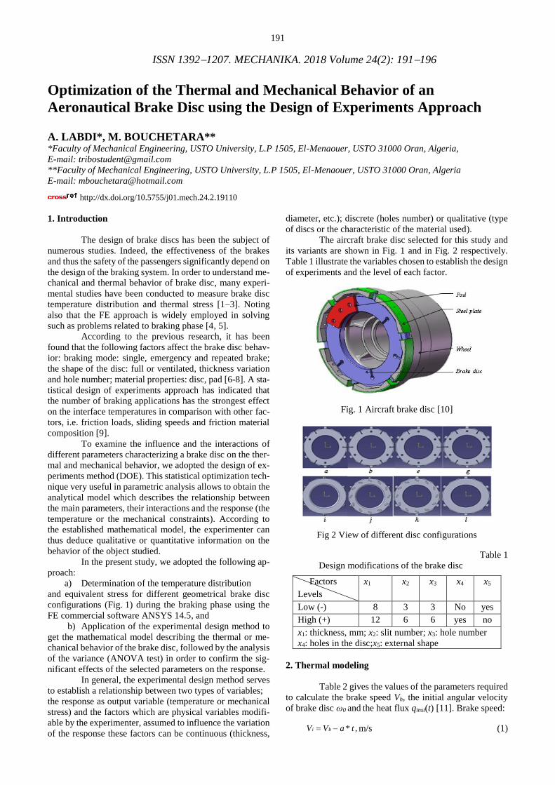
191 ISSN 13921207. MECHANIKA. 2018 Volume 24(2): 191196 Optimization of the Thermal and Mechanical Behavior of an Aeronautical Brake Disc using the Design of Experiments Approach A. LABDI*, M. BOUCHETARA** *Faculty of Mechanical Engineering, USTO University, L.P 1505, El-Menaouer, USTO 31000 Oran, Algeria, E-mail: [email protected] **Faculty of Mechanical Engineering, USTO University, L.P 1505, El-Menaouer, USTO 31000 Oran, Algeria E-mail: [email protected] http://dx.doi.org/10.5755/j01.mech.24.2.19110 1. Introduction The design of brake discs has been the subject of numerous studies. Indeed, the effectiveness of the brakes and thus the safety of the passengers significantly depend on the design of the braking system. In order to understand me- chanical and thermal behavior of brake disc, many experi- mental studies have been conducted to measure brake disc temperature distribution and thermal stress [1–3]. Noting also that the FE approach is widely employed in solving such as problems related to braking phase [4, 5]. According to the previous research, it has been found that the following factors affect the brake disc behav- ior: braking mode: single, emergency and repeated brake; the shape of the disc: full or ventilated, thickness variation and hole number; material properties: disc, pad [6-8]. A sta- tistical design of experiments approach has indicated that the number of braking applications has the strongest effect on the interface temperatures in comparison with other fac- tors, i.e. friction loads, sliding speeds and friction material composition [9]. To examine the influence and the interactions of different parameters characterizing a brake disc on the ther- mal and mechanical behavior, we adopted the design of ex- periments method (DOE). This statistical optimization tech- nique very useful in parametric analysis allows to obtain the analytical model which describes the relationship between the main parameters, their interactions and the response (the temperature or the mechanical constraints). According to the established mathematical model, the experimenter can thus deduce qualitative or quantitative information on the behavior of the object studied. In the present study, we adopted the following ap- proach: a) Determination of the temperature distribution and equivalent stress for different geometrical brake disc configurations (Fig. 1) during the braking phase using the FE commercial software ANSYS 14.5, and b) Application of the experimental design method to get the mathematical model describing the thermal or me- chanical behavior of the brake disc, followed by the analysis of the variance (ANOVA test) in order to confirm the sig- nificant effects of the selected parameters on the response. In general, the experimental design method serves to establish a relationship between two types of variables; the response as output variable (temperature or mechanical stress) and the factors which are physical variables modifi- able by the experimenter, assumed to influence the variation of the response these factors can be continuous (thickness, diameter, etc.); discrete (holes number) or qualitative (type of discs or the characteristic of the material used). The aircraft brake disc selected for this study and its variants are shown in Fig. 1 and in Fig. 2 respectively. Table 1 illustrate the variables chosen to establish the design of experiments and the level of each factor. Fig. 1 Aircraft brake disc [10] Fig 2 View of different disc configurations Table 1 Design modifications of the brake disc Factors Levels x1 x2 x3 x4 x5 Low (-) 8 3 3 No yes High (+) 12 6 6 yes no x1: thickness, mm; x2: slit number; x3: hole number x4: holes in the disc;x5: external shape 2. Thermal modeling Table 2 gives the values of the parameters required to calculate the brake speed Vh, the initial angular velocity of brake disc ω0 and the heat flux qinst(t) [11]. Brake speed: i b V V a*t, m/s (1)
Transcript of Optimization of the Thermal and Mechanical Behavior of an ...
191
ISSN 13921207. MECHANIKA. 2018 Volume 24(2): 191196
Optimization of the Thermal and Mechanical Behavior of an
Aeronautical Brake Disc using the Design of Experiments Approach
A. LABDI*, M. BOUCHETARA**
*Faculty of Mechanical Engineering, USTO University, L.P 1505, El-Menaouer, USTO 31000 Oran, Algeria,
E-mail: [email protected]
**Faculty of Mechanical Engineering, USTO University, L.P 1505, El-Menaouer, USTO 31000 Oran, Algeria
E-mail: [email protected]
http://dx.doi.org/10.5755/j01.mech.24.2.19110
1. Introduction
The design of brake discs has been the subject of
numerous studies. Indeed, the effectiveness of the brakes
and thus the safety of the passengers significantly depend on
the design of the braking system. In order to understand me-
chanical and thermal behavior of brake disc, many experi-
mental studies have been conducted to measure brake disc
temperature distribution and thermal stress [1–3]. Noting
also that the FE approach is widely employed in solving
such as problems related to braking phase [4, 5].
According to the previous research, it has been
found that the following factors affect the brake disc behav-
ior: braking mode: single, emergency and repeated brake;
the shape of the disc: full or ventilated, thickness variation
and hole number; material properties: disc, pad [6-8]. A sta-
tistical design of experiments approach has indicated that
the number of braking applications has the strongest effect
on the interface temperatures in comparison with other fac-
tors, i.e. friction loads, sliding speeds and friction material
composition [9].
To examine the influence and the interactions of
different parameters characterizing a brake disc on the ther-
mal and mechanical behavior, we adopted the design of ex-
periments method (DOE). This statistical optimization tech-
nique very useful in parametric analysis allows to obtain the
analytical model which describes the relationship between
the main parameters, their interactions and the response (the
temperature or the mechanical constraints). According to
the established mathematical model, the experimenter can
thus deduce qualitative or quantitative information on the
behavior of the object studied.
In the present study, we adopted the following ap-
proach:
a) Determination of the temperature distribution
and equivalent stress for different geometrical brake disc
configurations (Fig. 1) during the braking phase using the
FE commercial software ANSYS 14.5, and
b) Application of the experimental design method to
get the mathematical model describing the thermal or me-
chanical behavior of the brake disc, followed by the analysis
of the variance (ANOVA test) in order to confirm the sig-
nificant effects of the selected parameters on the response.
In general, the experimental design method serves
to establish a relationship between two types of variables;
the response as output variable (temperature or mechanical
stress) and the factors which are physical variables modifi-
able by the experimenter, assumed to influence the variation
of the response these factors can be continuous (thickness,
diameter, etc.); discrete (holes number) or qualitative (type
of discs or the characteristic of the material used).
The aircraft brake disc selected for this study and
its variants are shown in Fig. 1 and in Fig. 2 respectively.
Table 1 illustrate the variables chosen to establish the design
of experiments and the level of each factor.
Fig. 1 Aircraft brake disc [10]
Fig 2 View of different disc configurations
Table 1
Design modifications of the brake disc
Factors
Levels
x1 x2 x3 x4 x5
Low (-) 8 3 3 No yes
High (+) 12 6 6 yes no
x1: thickness, mm; x2: slit number; x3: hole number
x4: holes in the disc;x5: external shape
2. Thermal modeling
Table 2 gives the values of the parameters required
to calculate the brake speed Vh, the initial angular velocity
of brake disc ω0 and the heat flux qinst(t) [11]. Brake speed:
i bV V a* t , m/s (1)
192
Heat flux:
(t) 681902 75630.48* ,instq t w/m2 (2)
Table 2
Values of main simulation parameters
Total braking time tb ,s 9.00
Time step Δt ,s 0.01
Initial time ti ,s 0
Aircraft weight m ,kg 1050
Initial speed of landing Vi ,m/s 28.00
Aircraft deceleration dec ,m/s2 3.00
Braking distance Lb ,m 130
Wheel radius r,m 0.42
Flux distribution rate k 0.4
Contact surface (disc/pad) Ad ,mm2 13194.68
Applied force on the disc 𝐹𝑑,N 1512
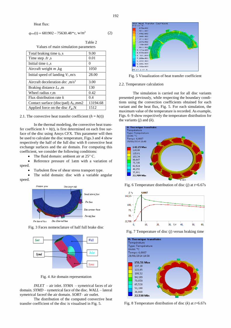
2.1. The convective heat transfer coefficient (h = h(t))
In the thermal modeling, the convective heat trans-
fer coefficient h = h(t), is first determined on each free sur-
face of the disc using Ansys CFX. This parameter will then
be used to calculate the disc temperature, Figs.3 and 4 show
respectively the half of the full disc with 8 convective heat
exchange surfaces and the air domain. For computing this
coefficient, we consider the following conditions:
The fluid domain: ambient air at 25° C.
Reference pressure of 1atm with a variation of
speed.
Turbulent flow of shear stress transport type.
The solid domain: disc with a variable angular
speed.
Fig. 3 Faces nomenclature of half full brake disc
Fig. 4 Air domain representation
INLET – air inlet. SYMA – symetrical faces of air
domain. SYMD – symetrical face of the disc. WALL – lateral
symetrical faceof the air domain. SORT– air outlet.
The distribution of the computed convective heat
transfer coefficient of the disc is visualised in Fig. 5.
Fig. 5 Visualization of heat transfer coefficient
2.2. Temperature calculation
The simulation is carried out for all disc variants
presented previously, while respecting the boundary condi-
tions using the convection coefficients obtained for each
variant and the heat flux, Fig. 5. For each simulation, the
maximum value of the temperature is recorded. As example,
Figs. 6–9 show respectively the temperature distribution for
the variants (j) and (k).
Fig. 6 Temperature distribution of disc (j) at t=6.67s
Fig. 7 Temperature of disc (j) versus braking time
Fig. 8 Temperature distribution of disc (k) at t=6.67s
193
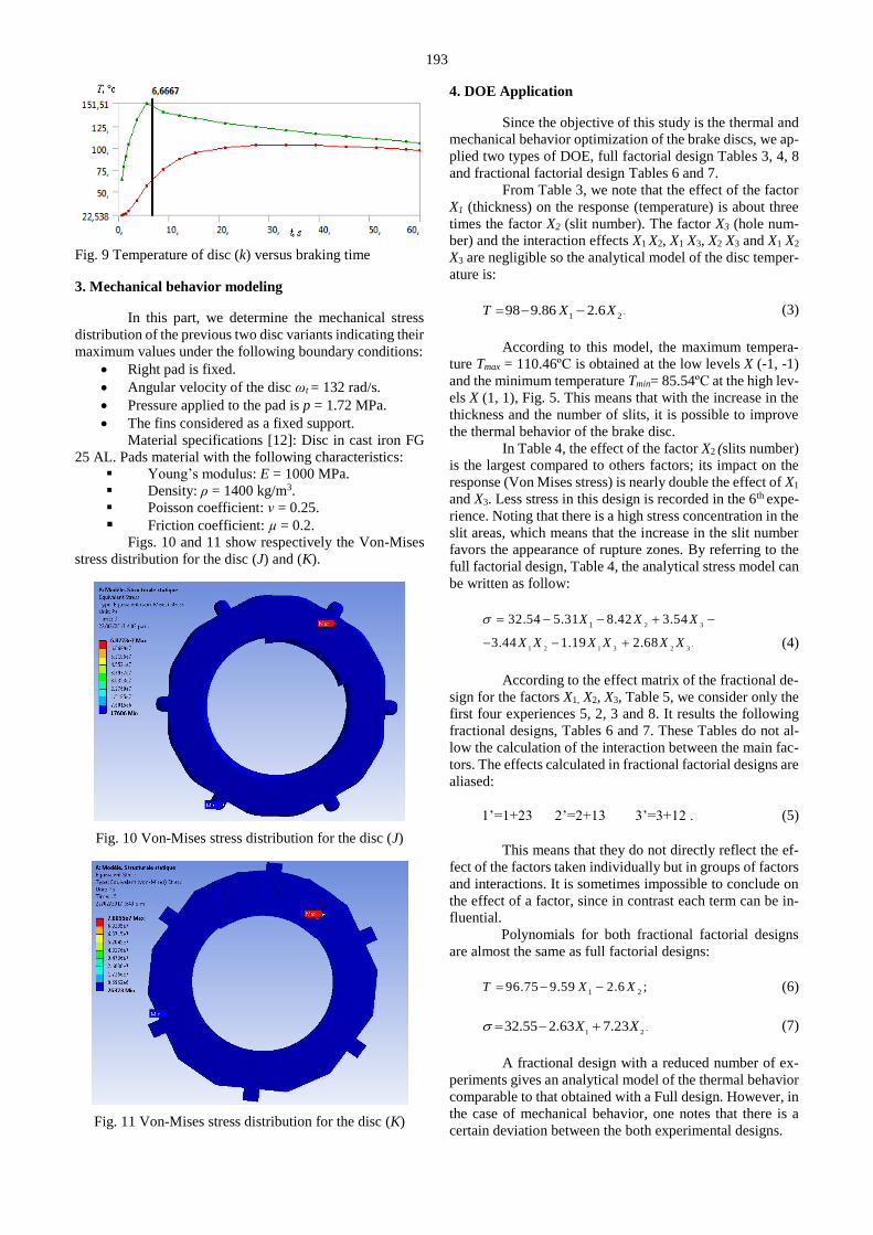
Fig. 9 Temperature of disc (k) versus braking time
3. Mechanical behavior modeling
In this part, we determine the mechanical stress
distribution of the previous two disc variants indicating their
maximum values under the following boundary conditions:
Right pad is fixed.
Angular velocity of the disc ωt = 132 rad/s.
Pressure applied to the pad is p = 1.72 MPa.
The fins considered as a fixed support.
Material specifications [12]: Disc in cast iron FG
25 AL. Pads material with the following characteristics:
Young’s modulus: E = 1000 MPa.
Density: ρ = 1400 kg/m3.
Poisson coefficient: ν = 0.25.
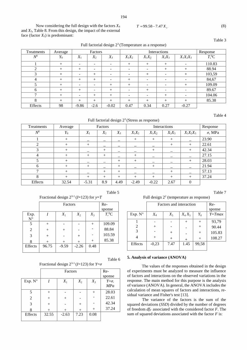
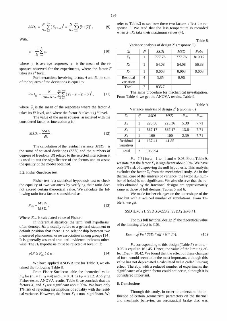
Friction coefficient: µ = 0.2. Figs. 10 and 11 show respectively the Von-Mises
stress distribution for the disc (J) and (K).
Fig. 10 Von-Mises stress distribution for the disc (J)
Fig. 11 Von-Mises stress distribution for the disc (K)
4. DOE Application
Since the objective of this study is the thermal and
mechanical behavior optimization of the brake discs, we ap-
plied two types of DOE, full factorial design Tables 3, 4, 8
and fractional factorial design Tables 6 and 7.
From Table 3, we note that the effect of the factor
X1 (thickness) on the response (temperature) is about three
times the factor X2 (slit number). The factor X3 (hole num-
ber) and the interaction effects X1 X2, X1 X3, X2 X3 and X1 X2
X3 are negligible so the analytical model of the disc temper-
ature is:
2.
1 98 9.86 2.6T X X (3)
According to this model, the maximum tempera-
ture Tmax = 110.46ºC is obtained at the low levels X (-1, -1)
and the minimum temperature Tmin= 85.54ºC at the high lev-
els X (1, 1), Fig. 5. This means that with the increase in the
thickness and the number of slits, it is possible to improve
the thermal behavior of the brake disc.
In Table 4, the effect of the factor X2 (slits number)
is the largest compared to others factors; its impact on the
response (Von Mises stress) is nearly double the effect of X1
and X3. Less stress in this design is recorded in the 6th expe-
rience. Noting that there is a high stress concentration in the
slit areas, which means that the increase in the slit number
favors the appearance of rupture zones. By referring to the
full factorial design, Table 4, the analytical stress model can
be written as follow:
2 3
1 2 1 3 2 3
1
.
32.54 5.31 8.42 3.54
3.44 1.19 2.68
X X X
X X X X X X
(4)
According to the effect matrix of the fractional de-
sign for the factors X1, X2, X3, Table 5, we consider only the
first four experiences 5, 2, 3 and 8. It results the following
fractional designs, Tables 6 and 7. These Tables do not al-
low the calculation of the interaction between the main fac-
tors. The effects calculated in fractional factorial designs are
aliased:
1’=1+23 2’=2+13 3’=3+12 . (5)
This means that they do not directly reflect the ef-
fect of the factors taken individually but in groups of factors
and interactions. It is sometimes impossible to conclude on
the effect of a factor, since in contrast each term can be in-
fluential.
Polynomials for both fractional factorial designs
are almost the same as full factorial designs:
1 2 96.75 9.59 2.6 ;T X X (6)
1 2. 32.55 2.63 7.23X X (7)
A fractional design with a reduced number of ex-
periments gives an analytical model of the thermal behavior
comparable to that obtained with a Full design. However, in
the case of mechanical behavior, one notes that there is a
certain deviation between the both experimental designs.
194
Now considering the full design with the factors X4
and X5, Table 8. From this design, the impact of the external
face (factor X5) is predominant:
5. 99.58 7.47T X (8)
Table 3
Full factorial design 23 (Temperature as a response)
Table 4
Full factorial design 23 (Stress as response)
Table 5
Fractional design 23-1 (I=123) for y=T
Factors Re-
sponse Exp.
N° I X1 X2 X3 T,0C
5
2
3
8
+
+
+
+
-
+
-
+
-
-
+
+
+
-
-
+
109.09
88.84
103.59
85.38
Effects 96.75 -9.59 -2.26 0.48
Table 6
Fractional design 23-1 (I=123) for Y=σ
Factors Re-
sponse Exp. N° I X1 X2 X3 Y=σ,
MPa
5
2
3
8
+
+
+
+
-
+
-
+
-
-
+
+
+
-
-
+
28.03
22.61
42.34
37.24
Effects 32.55 -2.63 7.23 0.08
Table 7
Full design 22 (temperature as response)
Factors and interaction Re-
sponse Exp. N° X4 X5 X4 X5 Y0 Y=Tmax
1
2
3
4
-
+
-
+
-
-
+
+
+
-
-
+
+
+
+
+
93,79
90.44
105.83
108.27
Effects -0,23 7.47 1.45 99,58
5. Analysis of variance (ANOVA)
The values of the responses obtained in the design
of experiments must be analyzed to measure the influence
of factors and interactions on the observed variations in the
response. The main method for this purpose is the analysis
of variance (ANOVA). In general, the ANOVA includes the
calculation of mean squares of factors and interactions, re-
sidual variance and Fisher's test [13].
The variance of the factors is the sum of the
squared deviations (SSD) divided by the number of degrees
of freedom dfF associated with the considered factor F. The
sum of squared deviations associated with the factor F is:
Treatments Average Factors Interactions Response
N0 Y0 X1 X2 X3 X1X2 X1X3 X2X3 X1X2X3 T,0C
1 + - - - + + + - 110.83
2 + + - - - - + + 88.94
3 + - + - - + - + 103,59
4 + + + - + - - - 84,67
5 + - - + + - - + 109.09
6 + + - + - + - - 89.67
7 + - + + - - + - 104.06
8 + + + + + + + + 85.38
Effects 98 -9.86 -2.6 -0.02 0.47 0.34 0.27 -0.27
Treatments Average Factors Interactions Response
N0 Y0 X1 X2 X3 X1X2 X1X3 X2X3 X1X2X3 σ, MPa
1 + _ _ _ + + + _ 23.90
2 + + _ _ _ _ + + 22.61
3 + _ + _ _ + _ + 42.34
4 + + + _ + _ _ _ 27.15
5 + _ _ + + _ _ + 28.03
6 + + _ + _ + _ _ 21.94
7 + _ + + _ _ + _ 57.13
8 + + + + + + + + 37.24
Effects 32.54 -5.31 8.9 4.49 -2.49 -0.22 2.67 0
195
2 2
1 1
,i
i i
Nn Nn
iF F F i
n ni i
iN NSSD E y y
N N
(9)
With:
,
1
1
N
i i
i
y yN
(10)
where y is average response; iy is the mean of the re-
sponses observed for the experiments, where the factor F
takes its i th level.
For interactions involving factors A and B, the sum
of the squares of the deviations is equal to:
2
1 1.,
i NnijNn
ijf
i j
ig
i jA iB
NSSD y y y y
Nn Nn
(11)
where ij
y is the mean of the responses where the factor A
takes its ith level, and where the factor B takes its j th level.
The value of the mean squares, associated with the
considered factor or interaction x is:
.x
x
x
SSDMSD
df (12)
The calculation of the residual variance MSDr is
the sums of squared deviations (SSD) and the numbers of
degrees of freedom (df) related to the selected interactions it
is used to test the significance of the factors and to assess
the quality of the model obtained.
5.2. Fisher-Snedecor test
Fisher test is a statistical hypothesis test to check
the equality of two variances by verifying their ratio does
not exceed certain theoretical value. We calculate the fol-
lowing ratio for a factor x considered as:
r
MSD ,MSD
x
obsF (13)
Where obsF is calculated value of Fisher.
In inferential statistics, the term "null hypothesis"
often denoted H0 is usually refers to a general statement or
default position that there is no relationship between two
measured phenomena, or no association among groups [14].
It is generally assumed true until evidence indicates other-
wise. The H0 hypothesis must be rejected at level α if:
( ) .obs
Fp F (14)
We have applied ANOVA test for Table 3, we ob-
tained the following Table 8.
From Fisher Snedecor table the theoretical value
Fth for (n1 = 1, n2 = 4) and α = 0.01, is Fth = 21.2. Applying
Fisher-test to ANOVA results, Table 8, we conclude that the
factors X1 and X2 are significant about 99%. We have only
1% risk of rejecting assumptions of equality with the resid-
ual variance. However, the factor X3 is non- significant. We
refer to Table.3 to see how these two factors affect the re-
sponse T. We read that the less temperature is recorded
when X1, X2 take their maximum values (+).
Table 8
Variance analysis of design 23 (response T)
iX df SSDi MSD Fobs
1X 1 777.76 777.76 810.17
2X 1 54.08 54.08 56.33
3X 1 0.003 0.003 0.003
Residual
variation
4 3.85 0.96
Total 7 835.7
The same procedure for mechanical investigation.
From Table 4, we get the ANOVA results, Table 9.
Table 9
(response σ) 32Variance analysis of design
iX df SSDi MSD obsF theoF
1X 1 225.36 225.36 5.38 7.71
2X 1 567.17 567.17 13.6 7.71
3X 1 100 100 2.39 7.71
Residual
variation
4 167.41 41.85
Total 7 1055.94
Fth =7.71 for n1=1, n2=4 and α=0.05. From Table 9,
we note that the factor X2 is significant about 95%. We have
only 5% risk of disproving the null hypothesis. This analysis
excludes the factor X1 from the mechanical study. As in the
thermal case of the analysis of variance, the factor X3 (num-
ber of holes) is not significant. We also observe that the re-
sults obtained by the fractional designs are approximately
same as those of full designs, Tables 5 and 6.
We made further changes on the outer shape of the
disc but with a reduced number of simulations. From Ta-
ble.8, we get:
SSD X4=0.21, SSD X5=223.2, SSDX4 X5=8.41.
For this full factorial design 22 the theoretical value
of the limiting effect is [15]:
( * * / * ).flim th r rE F SSD dff N df (15)
Fth corresponding to this design (Table.7) with α =
0.05 is equal to 161.45. Hence, the value of the limiting ef-
fect Ef,lim = 18.42. We found that the effect of these changes
of form would seem to be the most important, although this
value has not depreciated a calculated value called limiting
effect. Thereby, with a reduced number of experiments the
significance of a given factor could not occur, although it is
considered important.
6. Conclusions
Through this study, in order to understand the in-
fluence of certain geometrical parameters on the thermal
and mechanic behavior, an aeronautical brake disc was
196
taken making some modifications , we found that each var-
iant behaves thermally and mechanically different, to deter-
mine what are the factors influencing this behavior, the ex-
perimental design method was applied, it allowed us to
make three full factorial designs and two fractional designs,
it was possible also to write a mathematical model for each
of these designs; with ANOVA and Fisher test it was found
that among the factors selected in this study, the thickness
and the slit number were the most influential factors for the
thermal performance of the disc. However, for mechanical
behavior, the slit number was the most influential factor.
References
1. Chung, W.S.; Jung, S. P.; Park, T.W. 2010. Numeri-
cal analysis method to estimate thermal deformation of
a ventilated disc for automotives, Journal of Mechanical
Science and Technology 24: 2189-2195.
https://doi.org/10.1007/s12206-010-0905-3
2. Shahzamanian, M.M.; al. 2010. Finite element analysis
of thermoelastic contact problem in functionally graded
axisymmetric brake disks, Composite Structures 92:
1591-1602.
https://doi.org/10.1016/j.ijsolstr.2011.05.003.
3. Okamura, T.; Yumoto, H. 2006. Fundamental Study
on Thermal Behavior of Brake Discs, SAE Technical
Paper 01-3203.
https://doi.org/10.4271/2006-01-3203.
4. Gao, C.H; Lin, X.Z. 2002. Transient temperature field
analysis of a brake in a non-axisymmetric three-dimen-
sional model, Journal of Materials Processing Technol-
ogy 129(1-3): 513–517.
https://doi.org/10.1016/S0924-0136(02)00622-2.
5. Li, J.Y.; Barber, J.R. 2002. Solution of transient ther-
moelastic contact problems by the fast speed expansion
method, Wear 265(3-4):402–410.
https://doi.org/10.1016/j.wear.2007.11.010.
6. Adamowicz, A.; Grzes, P. 2002. Analysis of disc brake
temperature distribution during single braking under
non-axisymmetric load, Applied Thermal Engineering
31: 1003-1012.
https://doi.org/10.1016/j.applthermaleng.2010.12.016.
7. Duzgun, M. 2002. Investigation of thermo-structural
behaviours of different ventilation applications on brake
discs. Journal of Mechanical Science and Technology
26: 235-240.
http://doi.org/10.1007/s12206-011-0921-y.
8. Belhocine, A.; Bouchetara, M. 2013. Thermomechan-
ical Behaviour of Dry Contacts in Disc Brake Rotor with
a Grey Cast Iron Composition, Thermal Science 17, 2:
599-609.
https://doi.org/10.2298/TSCI110826141B.
9. Qi, H. S; A. Day, A. J. 2007. Investigation of disc/pad
interface temperatures in friction braking, Wear 262:
505- 513.
https://doi.org/10.1016/j.wear.2006.08.027.
10. Djafri, M. 2010.Etude du comportement thermoméca-
nique des disques de frein d’un avion léger, Faculty of
Mechanical Engineering, USTO University, Oran, Al-
geria.
11. Mackin, T. J.2002.Thermal cracking in disc brakes, en-
gineering failure analyse, Thesis, University of Illinois
at Urbara -champaign USA.9:63-76.
https://doi.org/10.1016/S1350-6307(00)00037-6.
12. Choi, J.H; Lee, I. 2003.Finite element analysis of tran-
sient thermoelastic behaviours in disk brakes, Departe-
ment of Aerospace, Korea,Advanced Institute of Sci-
ence and Technology, Journal of thermal stress 26(3):
223-244.
https://doi.org/10.1080/713855891.
13. Droesbeke, J.J; Fine, J.; Saporta, G. 1997. Plans
d’expériences - Applications à l’entreprise. Ed. TECH-
NIP.
14. Everitt, B.1998. The Cambridge Dictionary of Statis-
tics. Cambridge University Press. ISBN 0521593468.
15. Vivier, S. 2002.Stratégies d’optimisation par la méthode
des plans d’expériences et application aux dispositifs
électrotechniques modélisés par éléments finis. Thèse de
doctorat, Ecole Centrale de Lille Université des Sciences
et Technologies de Lille, chapitre I, p.60. Available from
Internet:
https://tel.archives-ouvertes.fr/tel-00005822/document.
A. Labdi, M. Bouchetara
OPTIMIZATION OF THE THERMAL AND
MECHANICAL BEHAVIOR OF AN AERONAUTICAL
BRAKE DISC USING THE DESIGN OF
EXPERIMENTS APPROACH
S u m m a r y
The construction of the brake discs is the subject of
numerous studies in the field of automotive, railway and
aviation. Indeed, it involves the safety of passengers, which
is a primary criterion. The research has focused on the con-
tact of two rubbing parts. So various phenomena may occur
such as the rise in temperature, wear and noise emissions. In
this study, we chose different geometric disc models de-
signed in 3D using Solid Works software, which are im-
ported ANSYS to do the evaluation of the heat transfer co-
efficients using ANSYS CFX code. Then we proceed to the
analysis of the transient thermal behavior of each model and
the determination of the equivalent stress. The simulation
results provided by the ANSYS software are used to estab-
lish several designs of experiments for each one we write
the corresponding mathematical model, then we apply
ANOVA method and fisher ‘s analysis to determine the in-
fluential factors.
Keywords: Brake disc - heat transfer- Ansys- Von Mises-
Design of Experiments -Anova.
Received September 24, 2017
Accepted April 18, 2018