OPTIMIZATION OF LOCATIONS OF VORONOI GRID POINTS IN ...
235
OPTIMIZATION OF LOCATIONS OF VORONOI GRID POINTS IN RESERVOIR SIMULATION A THESIS SUBMITTED TO THE GRADUATE SCHOOL OF NATURAL AND APPLIED SCIENCES OF MIDDLE EAST TECHNICAL UNIVERSITY BY ULVI RZA-GULIYEV IN PARTIAL FULFILLMENT OF THE REQUIREMENTS FOR THE DEGREE OF MASTER OF SCIENCE IN PETROLEUM AND NATURAL GAS ENGINEERING SEPTEMBER 2015
Transcript of OPTIMIZATION OF LOCATIONS OF VORONOI GRID POINTS IN ...

OPTIMIZATION OF LOCATIONS OF VORONOI GRID POINTS IN RESERVOIR SIMULATION
A THESIS SUBMITTED TO THE GRADUATE SCHOOL OF NATURAL AND APPLIED SCIENCES
OF MIDDLE EAST TECHNICAL UNIVERSITY
BY
ULVI RZA-GULIYEV
IN PARTIAL FULFILLMENT OF THE REQUIREMENTS FOR
THE DEGREE OF MASTER OF SCIENCE IN
PETROLEUM AND NATURAL GAS ENGINEERING
SEPTEMBER 2015


Approval of the thesis:
OPTIMIZATION OF LOCATIONS OF VORONOI GRIDS
IN RESERVOIR SIMULATION
submitted by ULVI RZA-GULIYEV in partial fulfillment of the requirements for the degree of Masters of Science in Petroleum and Natural Gas Engineering
Department, Middle East Technical University by,
Prof. Dr. Gülbin Dural Ünver _________________ Dean, Graduate School of Natural and Applied Sciences
Prof. Dr. Mustafa Verşan Kök _________________ Head of Department, Petroleum and Natural Gas Eng. Dept.
Prof. Dr. Çaglar Sınayuç _________________
Supervisor, Petroleum and Natural Gas Eng. Dept., METU
Examining Committee Members:
Prof. Dr. Mustafa Verşan Kök _________________ Petroleum and Natural Gas Engineering Dept., METU
Asst. Prof. Dr. Çaglar Sınayuç _________________ Petroleum and Natural Gas Engineering Dept., METU
Prof. Dr. Mahmut Parlaktuna _________________ Petroleum and Natural Gas Engineering Dept., METU Asst. Prof. Dr. İsmail Durgut _________________ Petroleum and Natural Gas Engineering Dept., METU Asst. Prof. Dr. Emre Artun _________________ Petroleum and Natural Gas Engineering Dept., METU NCC Date: 01.09.2015

iv
I hereby declare that all information in this document has been obtained and
presented in accordance with academic rules and ethical conduct. I also declare
that, as required by these rules and conduct, I have fully cited and referenced
all material and results that are not original to this work.
Name, Last Name: Ulvi, Rza-Guliyev
Signature:

v
ABSTRACT
OPTIMIZATION OF LOCATIONS OF VORONOI GRID POINTS IN
RESERVOIR SIMULATION
Rza-Guliyev, Ulvi
M.S., Department of Petroleum and Natural Gas Engineering
Supervisor: Asst. Prof. Dr. Çağlar Sınayuç
September 2015, 216 pages
Reservoir simulations are computer models that can imitate real world reservoir
behavior under different circumstances, therefore making it possible for reservoir
engineers to make sensitivity studies in order to assess different scenarios. These
models discretize the reservoir into smaller blocks either using structured grids or
unstructured grids. The application of regular structured grids to correctly map
reservoir's geological structure can be very difficult, if not nearly impossible.
Unstructured grids can be more convenient for those cases. Voronoi gridding
technique creates unstructured grids such that the boundary of two grids is normal to
the line connecting Voronoi particles that represents the grids. So that it would be
convenient to calculate the transmissibility on the block boundaries.
In this study instead of placing the Voronoi particles randomly, or in a regular
fashion, the properties of the reservoir such as permeability anisotropy, orientation of
the permeability vectors, heterogeneity of the petrophysical properties, and well
locations and types were taken into consideration in the placement of Voronoi
particles. A three-step algorithm, created in this thesis and written using Matlab
software, takes into account the high resolution petrophysical properties in a finer
static mesh, together with permeability anisotropy ratio and orientation and well

vi
location. This algorithm generates initial distribution of grid points that honors
permeability anisotropy, then assigns each grid point an error value, which is
dependent on grid point placement, and tries to minimize this error by moving bad
points onto better locations. The error gets lower as the Voronoi grids and the
background finer static mesh agrees with each other. Finally, after each grid point's
location is chosen grid points related to vertical and horizontal wells and fault are
added. Algorithm was implemented on six cases of different complexity and then
generated Voronoi grid blocks were used in a simple, single phase simulator to show
the effects of the optimized grids. It was seen that the developed code during the
study can match the given input static model and can reduce the number of grid
blocks required to model a hydrocarbon reservoir.
Key words: Voronoi, PEBI, reservoir simulation, optimization

vii
ÖZ
REZERVUAR SİMÜLASYONUNDA VORONOİ IZGARA NOKTALARININ
YERLERİNİN OPTİMİZASYONU
Rza-Guliyev, Ulvi
Yüksek Lisans, Petrol ve Doğal Gaz Mühendisliği Bölümü
Tez Yöneticisi: Yrd. Doç. Dr. Çağlar Sınayuç
Eylül 2015, 216 sayfa
Rezervuar simülasyonları gerçek saha davranışlarını farklı durumlarda taklit eden ve
bu sayede rezervuar mühendislerinin farklı senaryoları değerlendirmek için
hassasiyet çalışması yapmasını mümkün kılan bilgisayar modelleridir. Bu modeller
rezervuarı küçük bloklara yapılandırılmış bloklar halinde ya da yapılandırılmamış
bloklar halinde ayırırlar. Rezervuarın jeolojik yapısını doğru şekilde tanımlamak için
yapılandırılmış blokların kullanımı imkansız olmasa bile çok zordur.
Yapılandırılmamış bloklar bu durumda çok daha uygun olabilir. Voronoi ızgara
yöntemi ile elde edilen yapılandırılmamış bloklar arasındaki sınır, iki bloğu
birleştiren ve bloğu temsil eden parçacıkları birleştiren doğruya diktir. Bu sayede
blok sınırındaki iletgenliği hesaplamak daha kolay olmaktadır.
Bu çalışmada Voronoi parçacıklarını rastgele ya da düzenli şekilde yerleştirmek
yerine, rezervuarın geçirgenlik eşyönsüzlüğü, geçirgenlik vektörlerinin yönelimi,
petrofiziksel özelliklerin heterojenliği, kuyu yer ve tipleri gibi özellikleri göz önüne
alınarak voronoi parçacıklarının yerleri belirlenmiştir. Yüksek çözünürlüklü ince
statik bir ızgarada yer alan petrofiziksel özellikler, geçirgenlik eşyönsüzlük oranı ve
yönelimi ile kuyu yerlerini kullanan üç aşamalı bir Matlab kodu bu amaç için
yazılmıştır. Algoritma parçacıkların ilk dağılımını geçirgenlik eşyönsüzlüğü


viii
değerine bağlı olarak gerçekleştirmektedir. Yazılım voronoi parçacıklarının en
uygun yerlerini bir hata en aza indirme yöntemi ile belirlemektedir. Hata Voronoi
blokları ile ince statik ızgara ile verilen özellik sınırlarının birbirleri ile örtüşmesi ile
azalmaktadır. Son olarak, parçacıkların yerleri belirlendikten sonra dikey ve yatay
kuyular ile fay hatları eklenmektedir. Basit, tek fazlı bir simülatör kullanılarak altı
farklı durum için en uygun hale getirilmiş ızgaraların etkisi görülmüştür. Çalışma
sırasında geliştirilen kodun verilen statik model ile örtüştüğü ve bir hidrokarbon
rezervuarını modellemek için gerekli blok sayısını azalttığı görülmüştür.
Anahtar kelimeler: Voronoi, PEBI, rezervuar simülasyon, optimizasyon

ix
ACKNOWLEDGEMENTS
I would like to thank:
My supervisor Prof. Dr. Çağlar Sınayuç for his assistance and continuous help
throughout making of this thesis;
Middle East Technical University Petroleum and Natural Gas Engineering
Department for their dedication to the work and always being there if any help is
required;
My family for their continuous support and faith in me;
My friends Said Akhundov, Tugce Bayram, Nijat Mutallimov, Rashad Mutallimov,
Fuad Rahimov, Avaz Alaskarov and Osman Quliyev for their interesting ideas that
put me on the right track throughout making of this thesis.

x
TABLE OF CONTENTS
ABSTRACT ................................................................................................................. v
ÖZ .............................................................................................................................. vii
ACKNOWLEDGEMENTS ........................................................................................ ix
TABLE OF CONTENTS ............................................................................................. x
LIST OF TABLES .................................................................................................... xiii
LIST OF FIGURES .................................................................................................. xiv
CHAPTERS
1. INTRODUCTION ................................................................................................ 1
2. RESERVOIR SIMULATION .............................................................................. 5
2.1. Introduction ................................................................................................... 5
2.2. Motivation to use reservoir simulation .......................................................... 7
2.3. Gridding techniques....................................................................................... 7
2.3.1. Structured Grids................................................................................... 8
2.3.1.1. Cartesian Grid ......................................................................... 8
2.3.1.2. Cylindrical Grid ...................................................................... 9
2.3.1.3. Hexagonal Grid .................................................................... 10
2.3.1.4. Triangular Grid ..................................................................... 11
2.3.2. Untructured Grids .............................................................................. 11
2.3.2.1. Voronoi Grid ........................................................................ 12
2.3.2.2. Truncated Grid...................................................................... 13
2.3.2.3. Curvilinear Grid.................................................................... 14
2.3.3. Hybrid Grid ....................................................................................... 15
3. VORONOI GRID BLOCKS .............................................................................. 17
3.1. Introduction ................................................................................................. 17
3.2. Motivation to use Voronoi grids.................................................................. 20
3.3. Voronoi grid generation algorithm .............................................................. 21
3.3. Use of Voronoi grid in reservoir simulation ................................................ 23

xi
4. RESERVOIR HETEROGENEITIES AND ANISOTROPY ............................. 27
4.1. Introduction ................................................................................................. 27
4.2. Channeling ................................................................................................... 28
4.3. Anisotropy ................................................................................................... 31
5. OPTIMIZATION ............................................................................................... 35
5.1. Introduction to optimization ........................................................................ 35
5.2. Classes of optimization algorithms ............................................................. 36
5.3. Evolutionary algorithms .............................................................................. 39
6. PROBLEM STATEMENT ................................................................................ 43
7. METHODOLOGY ............................................................................................. 45
7.1. Introduction ................................................................................................. 45
7.2. Step One (generation of initial population of grid points) .......................... 46
7.3. Step Two (movement of the bad grid points) .............................................. 49
7.4. Step Three (adding of grid points related to wells and faults)..................... 57
7.4.1. Treatment of vertical wells ................................................................ 57
7.4.2. Treatment of horizontal wells and faults ........................................... 59
8. RESULTS OF STUDY ...................................................................................... 61
8.1. Introduction ................................................................................................. 61
8.2. Cases ............................................................................................................ 62
8.2.1. Case One (no anisotropy, no heterogeneities, one vertical well) ...... 62
8.2.2. Case Two (anisotropy, no heterogeneities, one vertical well) ........... 72
8.2.3. Case Three (anisotropy, straight channel, one vertical well) ............ 77
8.2.4. Case Four (anisotropy, deviated channel, one vertical well) ............. 83
8.2.5. Case Five (anisotropy, four different regions, one vertical well) ...... 87
8.2.6. Case Six (anisotropy, no heterogeneities, fault and horizontal well) 92
8.3. Effects of inputs on final results .................................................................. 95
8.3.1. Effect of number of grid points ......................................................... 96
8.3.2. Effect of number of moving grid points ............................................ 97
8.3.3. Effect of limit of movement of grid points ........................................ 98
8.3.4. Effect of distance of movement of grid points .................................. 99
9. CONCLUSION ................................................................................................ 101
10. PROPOSITION FOR FUTURE STUDIES ................................................... 103

xii
BIBLIOGRAPHY ................................................................................................ 105
APPENDICES
A. SOURCE CODE ............................................................................................. 113
B. CASE 2 FLUID FLOW SIMULATION RUN ................................................ 193
C. CASE 3 FLUID FLOW SIMULATION RUN ............................................... 199
D. CASE 4 FLUID FLOW SIMULATION RUN .............................................. 205
E. CASE 5 FLUID FLOW SIMULATION RUN ............................................... 211

xiii
LIST OF TABLES
TABLE
8.1. Description of the cases ...................................................................................... 61

xiv
LIST OF FIGURES
FIGURES
2.1. Main stages of generation of reservoir simulators ................................................ 7
2.2. Representation of geological feature using structured Cartesian grid with
refinement (a) versus unstructured grid (b) ................................................................. 8
2.3. Cartesian grid in 2D (a) and 3D (b).. .................................................................... 9
2.4. Local grid refinement in regular Cartesian grid .................................................... 9
2.5. Cylindrical grid in two dimensions with local refinement (a) and three
dimensions (b) ............................................................................................................ 10
2.6. Example on hexagonal grid in two dimensions .................................................. 10
2.7. Example on triangular grid in two dimensions ................................................... 11
2.8. Example on Voronoi grid in two dimensions ..................................................... 12
2.9. Truncated grid ..................................................................................................... 13
2.10. Example on curvilinear grid type ...................................................................... 14
2.11. Example on hybrid grids ................................................................................... 15
3.1. Example on usage of hybrid gridding in reservoir simulation ............................ 18
3.2. Example on local grid refinement ....................................................................... 19
3.3. Voronoi grid and Delaunay mesh ....................................................................... 20
3.4. Common grid techniques that can be associated with Voronoi .......................... 21
4.1. Reservoir heterogeneity classes .......................................................................... 28
4.2. Braided fluvial deposition system ....................................................................... 29
4.3. Meandering fluvial deposition system ................................................................ 30
4.4. Example on diagenetic changes .......................................................................... 32
5.1. Rough classification of optimization algorithms ................................................ 37
5.2. The basic cycle of evolutionary algorithms ........................................................ 39
7.1. Angle between permeability in y-direction and y-direction of the reservoir ...... 46
xv
7.2. First step example. Black rectangle - reservoir; green rectangle - area, where
grid points will be generated; red dot - starting point; a - reservoir length; b -
reservoir width ........................................................................................................... 47
7.3. Flowchart of step one .......................................................................................... 48
7.4. Example on results obtained from the step one. Blue area - reservoir: white area
- zone outside of reservoir .......................................................................................... 50
7.5. Example on petrophysical field .......................................................................... 51
7.6. Flowchart of step two .......................................................................................... 52
7.7. Zoom in of the orange rectangle from the figure 7.4. Green dots show property
points inside reservoir; red points show property points outside of reservoir; blue
dots are grid points ..................................................................................................... 53
7.8. Example on reservoir.. ........................................................................................ 55
7.9. Treating of vertical wells .................................................................................... 56
7.10. Treating of horizontal wells.. ............................................................................ 58
7.11. Treating of faults.. ............................................................................................. 59
8.1. Permeability field for cases #1, #2 and #6 (plotted using MATLAB) ................ 62
8.2. Results obtained after running of the first step for the case #1 (built in
MATLAB) ................................................................................................................ 63
8.3. Results obtained after running of the second step of case #2 (built in MATLAB)
.................................................................................................................................... 64
8.4. Error values for all generations of Case #1 ......................................................... 65
8.5. Results obtained for the case #1 (built in MATLAB) ......................................... 66
8.6. Pressure distribution after 5 days ........................................................................ 67
8.7. Pressure distribution after 10 days ...................................................................... 67
8.8. Pressure distribution after 15 days ...................................................................... 68
8.9. Pressure distribution after 20 days ...................................................................... 68
8.10. Pressure distribution after 25 days .................................................................... 69
8.11. Pressure distribution after 30 days .................................................................... 69
8.12. Pressure distribution after 35 days .................................................................... 70
8.13. Pressure distribution after 40 days .................................................................... 70
8.14. Pressure distribution after 45 days .................................................................... 71
8.15. Pressure distribution after 50 days .................................................................... 71

xvi
8.16. Results obtained after running of the first step for the case #2 (built in
MATLAB).. ............................................................................................................... 72
8.17. Results obtained after running of the second step of case #2(built in MATLAB)
.................................................................................................................................... 73
8.18. Error values for all generations of Case #2 ....................................................... 74
8.19. Results obtained for the case #2 (built in MATLAB)....................................... 75
8.20. Velocity field combined with the contour map of the distribution of the
pressures after 10 days of production for the second case (obtained with Surfer).. .. 76
8.21. Permeability field for case #3. Generated in MATLAB.. ................................. 76
8.22. Results obtained after running of the first step for the case #3 (built in
MATLAB).. ............................................................................................................... 78
8.23. Results obtained after running of the second step of case #3 (built in
MATLAB).. ............................................................................................................... 78
8.24. Error values for all generations of Case #3 ....................................................... 79
8.25. Results obtained for the case #3 (built in MATLAB)....................................... 80
8.26. Velocity field combined with the contour map of the distribution of the
pressures after 15 days of production for the third case (obtained with Surfer) ........ 81
8.27. Permeability field for case #4. Plotted in MATLAB ........................................ 82
8.28. Results obtained after running of the first step for the case #4 (built in
MATLAB).. ............................................................................................................... 83
8.29. Results obtained after running of the second step of case #4 (built in
MATLAB).. ............................................................................................................... 84
8.30. Error values for all generations of Case #4 ....................................................... 84
8.31. Results obtained for the case #4 (built in MATLAB)....................................... 85
8.32. Velocity field combined with the contour map of the distribution of the
pressures after 15 days of production for the fourth case (obtained with Surfer) ...... 86
8.33. Permeability field for case #5. Plotted in MATLAB ........................................ 87
8.34. Results obtained after running of the first step for the case #5 (built in
MATLAB).. ............................................................................................................... 88
8.35. Results obtained after running of the second step of case #5 (built in
MATLAB.. ................................................................................................................. 89
8.36. Error values for all generations of Case #5 ....................................................... 90
xvii
8.37. Results obtained for the case #5 (built in MATLAB) ....................................... 91
8.38. Velocity field combined with the contour map of the distribution of the
pressures after 25 days of production for the fifth case (obtained with Surfer)......... 91
8.39. Results obtained after running of the first step for the case #6 (built in
MATLAB).. ............................................................................................................... 92
8.40. Results obtained after running of the second step of case #6 (built in
MATLAB).. ............................................................................................................... 93
8.41. Error values for all generations of Case #6 ....................................................... 94
8.42. Results obtained for the case number six (built in MATLAB) ......................... 95
8.43. Comparing results with different number of blocks (obtained with MATLAB)
.................................................................................................................................... 96
8.44. Comparing results with different number of movements for each grid point
(obtained with MATLAB).. ....................................................................................... 97
8.45. Comparing results with different limits of movement (obtained with
MATLAB).. ............................................................................................................... 98
8.46. Comparing results with different distance of movement (obtained with
MATLAB).. ............................................................................................................... 99
B.1. Pressure distribution after 5 days ..................................................................... 193
B.2. Pressure distribution after 10 days ................................................................... 194
B.3. Pressure distribution after 15 days ................................................................... 194
B.4. Pressure distribution after 20 days ................................................................... 195
B.5. Pressure distribution after 25 days ................................................................... 195
B.6. Pressure distribution after 30 days ................................................................... 196
B.7. Pressure distribution after 35 days ................................................................... 196
B.8. Pressure distribution after 40 days ................................................................... 197
B.9. Pressure distribution after 45 days ................................................................... 197
B.10. Pressure distribution after 50 days ................................................................. 198
C.1. Pressure distribution after 5 days ..................................................................... 199
C.2. Pressure distribution after 10 days ................................................................... 200
C.3. Pressure distribution after 15 days ................................................................... 200
C.4. Pressure distribution after 20 days ................................................................... 201
C.5. Pressure distribution after 25 days ................................................................... 201

xviii
C.6. Pressure distribution after 30 days ................................................................... 202
C.7. Pressure distribution after 35 days ................................................................... 202
C.8. Pressure distribution after 40 days ................................................................... 203
C.9. Pressure distribution after 45 days ................................................................... 203
C.10. Pressure distribution after 50 days ................................................................. 204
D.1. Pressure distribution after 5 days ..................................................................... 205
D.2. Pressure distribution after 10 days ................................................................... 206
D.3. Pressure distribution after 15 days ................................................................... 206
D.4. Pressure distribution after 20 days ................................................................... 207
D.5. Pressure distribution after 25 days ................................................................... 207
D.6. Pressure distribution after 30 days ................................................................... 208
D.7. Pressure distribution after 35 days ................................................................... 208
D.8. Pressure distribution after 40 days ................................................................... 209
D.9. Pressure distribution after 45 days ................................................................... 209
D.10. Pressure distribution after 50 days ................................................................. 210
E.1. Pressure distribution after 0.5 days .................................................................. 211
E.2. Pressure distribution after 1 day ....................................................................... 212
E.3. Pressure distribution after 1.5 days .................................................................. 212
E.4. Pressure distribution after 2 days ..................................................................... 213
E.5. Pressure distribution after 2.5 days .................................................................. 213
E.6. Pressure distribution after 3 days ..................................................................... 214
E.7. Pressure distribution after 3.5 days .................................................................. 214
E.8. Pressure distribution after 4 days ..................................................................... 215
E.9. Pressure distribution after 4.5 days .................................................................. 215
E.10. Pressure distribution after 5 days ................................................................... 216
1
CHAPTER 1
INTRODUCTION
With the dramatic advancements in computers during last half of the century,
reservoir modeling became one of the most powerful tools in the hands of reservoir
engineers. By giving possibility to assess different ways of exploitation of reservoirs
before making a final decision, it gave opportunity to correctly evaluate all possible
outcomes and to produce petroleum in the most efficient way.
Reservoir modeling is a process of usage of petrophysical and geological data
obtained from different studies in the field in order to predict the behavior of the
fluids under different conditions (Lie and Mallison, 2010). It is done by creating a
model which is a simplification of the real reservoir. This model is discretized into a
great amount of grid blocks, between which flow is calculated using fundamental
laws of fluid flow.
One of the factors that effectiveness of reservoir simulation depends on is a choice of
gridding type. There are many different types of the gridding techniques that have
been used in reservoir simulation. In the early days of reservoir simulation, only a
limited amount of Cartesian grids was used because of limitations of computers'
calculating power and available memory. So there was no need in creating new
gridding techniques, and for some time reservoirs were simulated by using several
thousand Cartesian grid blocks. The development of computers, their calculating
power and memory resulted in the possibility to use greater amount of blocks,
therefore resolution of models increased. With this refinement of blocks, new
demand appeared to try to represent complex geological features and fluid flow in a

2
more accurate manner. That was the cause that resulted in the creation of new
gridding techniques.
Usually, gridding techniques are separated into two broad groups: structured and
unstructured gridding. Sometimes hybrid grids are taken as the third group. Group of
structured gridding types include Cartesian, cylindrical, hexagonal etc, while one of
the most popular type of unstructured grids is PEBI (PErpendicular BIsector) or
Voronoi grids. The difference between structured and unstructured grids is that
structured grid types imply same regular shape of all of the grid blocks (for example,
triangles, rectangles), while unstructured ones do not require that condition (Moog,
2013). This difference means that unstructured grids are more flexible, compared to
the structured ones, which means that it can be used less amount of blocks to
represent some geological entity in the model without losing accuracy (Heinemann
and Brand, 1989).
Majority of unstructured grids was introduced in 1980's in order to meet
specifications concerning flexible modeling. The main types of grids invented during
this period include Control Volume Finite Element (Forsyth, 1989), Voronoi grids
(Heinemann and Brand, 1989) and hybrid grids (Pedrosa and Aziz, 1985). Voronoi
grid type appeared to be useful, because it takes better sides from both structured and
unstructured grids: they were flexible, allowed usage of different grid types,
providing a smooth transition from Voronoi grids to other gridding types (Katzmayr
and Ganzer, 2009).
However, apart from obvious advantages of unstructured grids, they also have some
problems: different number of block sides, non-orthogonality to the flow (grid
orientation effects) and others.
Voronoi grid blocks are areas that are closer to its grid point than to any of the other
ones, and the grid consists of this type of blocks (Palagi and Aziz, 1994). This
definition means that by accurate placement of Voronoi grid points in the reservoir
3
simulation accurate mapping of reservoir structures could be done. This study
focuses on optimization of Voronoi grid blocks' locations for this reason.
Optimization problem implies choosing of one option from a group of possible
solutions to the problem in order to maximize or minimize predefined function. In
the case discussed in this thesis optimization problem is in obtaining of optimized
locations of predefined number of grid blocks in a reservoir simulation of a field
including heterogeneities and/or permeability anisotropy while minimizing sum of
errors in all of the Voronoi grids. Each grid block in the simulation in the study is
assigned an error value - coefficient of badness of its placement. This error depends
on the match of the Voronoi grids with finer static mesh of petrophysical properties.
The higher the error in the block, the higher priority it has in the line of points that
will be moved. By moving of these bad points, an attempt to find better locations to
minimize the error value, and therefore better placing of grid points can be obtained
without increasing the amount of them.
In order to solve optimization problem, an optimization algorithm is usually
required. Optimization algorithm is a number of instructions that are required to be
applied to the problem in the correct order in order to reach desired results. All
optimization algorithms can be divided into two broad groups: probabilistic and
deterministic optimization algorithms. Probabilistic algorithms are such algorithms
that have at least one process including generation of random numbers in one of the
steps. This means that for the same input this algorithm will be able to produce
different results. This type of optimization algorithms is usually used when
approximate steps in order to reach optimized state are not known beforehand, so it
is required to search for this state everywhere. However, if these steps are known,
then no random generation (or searching for the correct direction) is required and
deterministic algorithms can be used. As it may be understood from this,
deterministic algorithms will always give the same results for the same input values.
(Weise, 2011)

4
The algorithm created in this study shares some concepts with evolutionary
optimization algorithms that are related to the probabilistic group, but itself is related
to the deterministic group. It consists of three simple steps the first of which
generates predefined number of uniformly distributed initial population of grid
points; the second step tries to minimize sum of errors in all of the blocks by moving
grid points obtained from the first step; the last step takes result obtained in the step
two and adds grid points related to wells and/or faults. This algorithm is described in
details in "Methodology" chapter.
Next chapters provide more detailed information on the main subjects of this study:
reservoir simulation, Voronoi gridding, reservoir heterogeneities and anisotropy, and
optimization.

5
CHAPTER 2
RESERVOIR SIMULATION
2.1. Introduction
At any particular point in geologic time, there is only one real dispensation of
petrophysical properties in the reservoir. This dispensation is the result of a
complicated combined work of chemical, physical, and biological processes.
Notwithstanding the fact that sometimes physics of depositional processes and
processes, occurring after deposition, may be realized very well, engineers do not
absolutely understand each process and its interaction with the others, which in
combination with the inability to get the boundary and initial conditions results in
impossibility to obtain the real singular dispensation of the properties of the reservoir
that change with time. So the only way is to build numerical simulations that can
imitate the real change of reservoir properties with time. Therefore, engineers try to
build reservoir simulations so that they would correlate with all the obtained data.
They understand that usually the real dispensation of reservoir properties will not be
exactly the same as in the model prediction, but they try to get the results as close as
possible (Pyrcz and Deutsch, 2014).
In less words, reservoir simulation is the process of inferring the behavior of a real
reservoir from the performance of a model of that reservoir (Jensen et al., 1997).
First reservoir simulations were far from what we have today. Actually, they were
physical models - for example, boxes made out of glass and filled with sand, from
where fluid was passing allowing scientist/engineer to look and understand what is
happening there. These simulations were first used in the 1930s and were used for

6
getting idea of how water breakthrough occurs in wells of the reservoir that has been
waterflooded.
With advancements in computers from 1960s and later, reservoir simulations
changed from physical models to computer-based models. These models divided
existing reservoir into a number of connecting blocks and calculated the flow that
will occur between these blocks under different conditions. When computers were
just introduced, they had far less efficiency and power than what we have today -
this fact was limiting number of blocks that reservoir can be divided into, which
resulted in not so reliable results obtained after simulator was run. Nowadays,
simulators allow to create models of millions and even billions of blocks, which
makes results much more reliable (Islam et al., 2010).
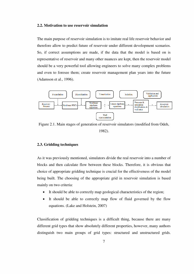
Figure 2.1 shows the main steps in the creation of the reservoir model as defined by
Odeh in 1982. Formulation stage here includes the introduction of assumptions
required to create a reservoir model in mathematical form. Then nonlinear partial
differential equations describing fluid flow are introduced, which are then undergo
stage of discretization and form a bunch of nonlinear algebraic equations. This
discretization can be done by applying Taylor series expansion (other techniques are
integral and variatonal methods (Aziz and Settari, 1979).
As it was already mentioned, discretization results in formation of nonlinear
algebraic equations, which in most of the cases require linearization in order to be
solved. Well representation is also required at this stage in order to add fluid
production/injection into equations that are still nonlinear.
After all previous steps are fulfilled, solutions can be obtained. These solutions
include distribution of both pressure and saturations and also flow rates of the
introduced wells. Validation step is just checking that no mistakes were made in the
previous step and in the source code of the simulator. After all these stages are done,
the simulator is ready to be used. (Islam et al., 2010)
7
2.2. Motivation to use reservoir simulation
The main purpose of reservoir simulation is to imitate real life reservoir behavior and
therefore allow to predict future of reservoir under different development scenarios.
So, if correct assumptions are made, if the data that the model is based on is
representative of reservoir and many other nuances are kept, then the reservoir model
should be a very powerful tool allowing engineers to solve many complex problems
and even to foresee them; create reservoir management plan years into the future
(Adamson et al., 1996).
Figure 2.1. Main stages of generation of reservoir simulators (modified from Odeh,
1982).
2.3. Gridding techniques
As it was previously mentioned, simulators divide the real reservoir into a number of
blocks and then calculate flow between these blocks. Therefore, it is obvious that
choice of appropriate gridding technique is crucial for the effectiveness of the model
being built. The choosing of the appropriate grid in reservoir simulation is based
mainly on two criteria:
It should be able to correctly map geological characteristics of the region;
It should be able to correctly map flow of fluid governed by the flow
equations. (Lake and Holstein, 2007)
Classification of gridding techniques is a difficult thing, because there are many
different grid types that show absolutely different properties, however, many authors
distinguish two main groups of grid types: structured and unstructured grids.
8
However, there are also grids that are not related to any of these groups. This
subchapter will discuss these grid types one by one.
2.3.1. Structured grids
There are different definitions of structured grids in the literature, including
"structured grid is a mesh type, consisting of many grid blocks of same geometrical
shape" (Moog, 2013) and "structured gridding is a mesh type consisting of blocks
with regular connectivity" (Castillo, 1991).
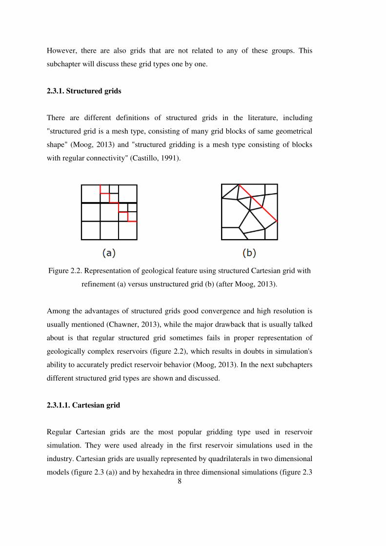
Figure 2.2. Representation of geological feature using structured Cartesian grid with
refinement (a) versus unstructured grid (b) (after Moog, 2013).
Among the advantages of structured grids good convergence and high resolution is
usually mentioned (Chawner, 2013), while the major drawback that is usually talked
about is that regular structured grid sometimes fails in proper representation of
geologically complex reservoirs (figure 2.2), which results in doubts in simulation's
ability to accurately predict reservoir behavior (Moog, 2013). In the next subchapters
different structured grid types are shown and discussed.
2.3.1.1. Cartesian grid
Regular Cartesian grids are the most popular gridding type used in reservoir
simulation. They were used already in the first reservoir simulations used in the
industry. Cartesian grids are usually represented by quadrilaterals in two dimensional
models (figure 2.3 (a)) and by hexahedra in three dimensional simulations (figure 2.3
9
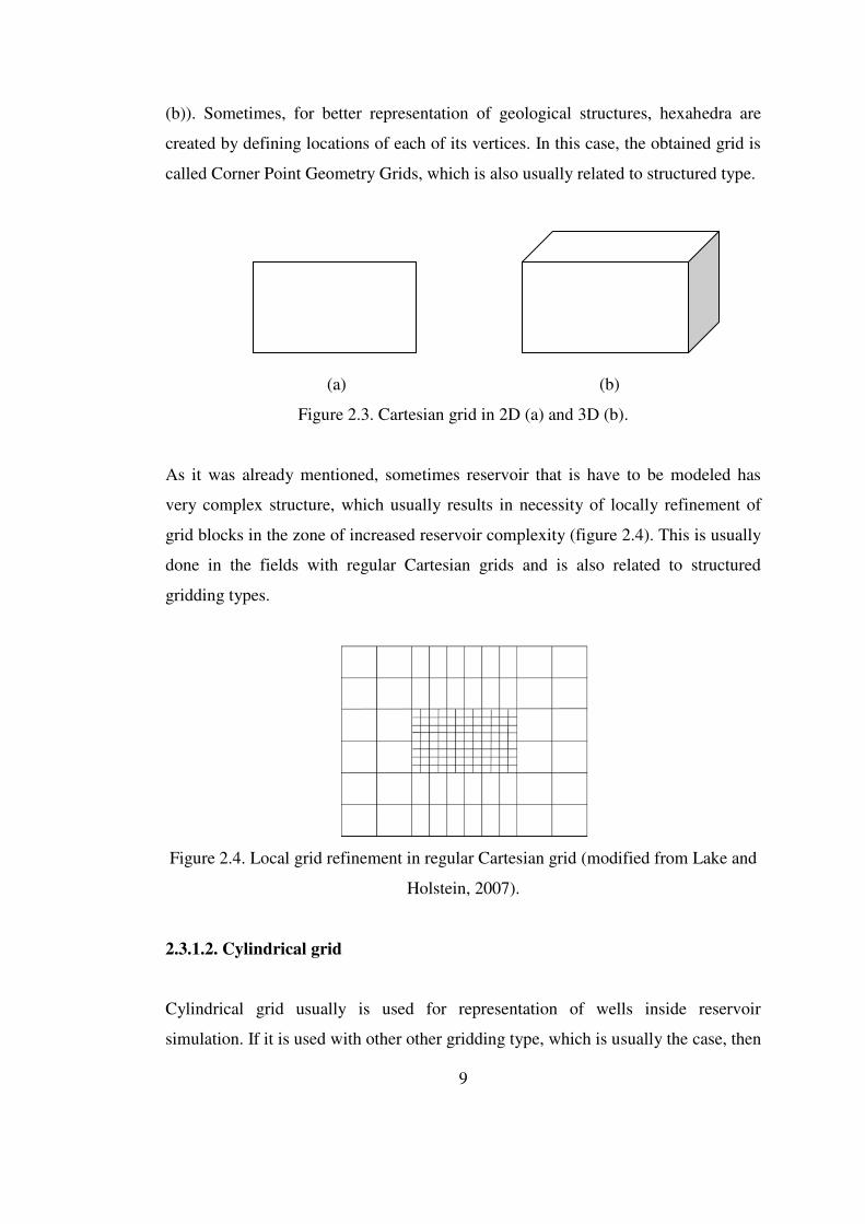
(b)). Sometimes, for better representation of geological structures, hexahedra are
created by defining locations of each of its vertices. In this case, the obtained grid is
called Corner Point Geometry Grids, which is also usually related to structured type.
(a) (b)
Figure 2.3. Cartesian grid in 2D (a) and 3D (b).
As it was already mentioned, sometimes reservoir that is have to be modeled has
very complex structure, which usually results in necessity of locally refinement of
grid blocks in the zone of increased reservoir complexity (figure 2.4). This is usually
done in the fields with regular Cartesian grids and is also related to structured
gridding types.
Figure 2.4. Local grid refinement in regular Cartesian grid (modified from Lake and
Holstein, 2007).
2.3.1.2. Cylindrical grid
Cylindrical grid usually is used for representation of wells inside reservoir
simulation. If it is used with other other gridding type, which is usually the case, then

10
it becomes a hybrid grid which is described in the subchapter 2.3.3.1. It can be both
used in two and three dimensional reservoir simulations (figure 2.5).
(a) (b)
Figure 2.5. Cylindrical grid in two dimensions with local refinement (a) and three
dimensions (b) (modified from Kaufmann, 2006 and Angelo et al., 2002).
2.3.1.3. Hexagonal grid
Hexagonal grid is used rarely in reservoir simulation. The first proposal of
application of hexagonal grid to the reservoir simulation was in the work of Pruess
and Bodvarsson (Pruess and Bodvarsson, 1983).
Figure 2.6. Example on hexagonal grid in two dimensions.
From the definition of structured grids, hexagonal grids must be related to them,
however in reality hexagonal structure is usually obtained by applying of
unstructured gridding techniques. As an example, typical shapes of Voronoi grids in

11
two dimensions are hexagons, while in three dimensions they are hexagonal prisms
(figure 2.6).
One of the successful applications of structured hegagonal grid is described in the
work of Wadsley et al. (Wadsley et al., 1990). He and his companions used
hexagonal grids in order to model fluvial architecture with subsequent simulation of
reservoir under production. Among the pluses of hexagonal grids, they mention the
fact that hexagonal grids help to overcome grid orientation effects.
2.3.1.4. Triangular Grid
Triangular grids are used very rarely in reservoir modeling. This is due to they
usually correspond to unstructured Voronoi gridding (Delaunay triangulation), which
is more persistent to grid changes. Other cause of its rare usage is that they usually
result in, what some authors call, "sliver" blocks that have little volume but big area
of surface (Lake and Holstein, 2007).
Figure 2.7. Example on triangular grid in two dimensions.
In two dimensions triangular grid is represented by triangles, while in three
dimensions they exist as tetrahedra (figure 2.7).
2.3.2. Unstructured Grids
As it was already mentioned, as distinct from structured gridding types, unstructured
ones do not have particular shape, which results in its flexibility that makes it

12
possible to more accurately represent geologic entities in the model (figure 2.2).
Other differences between these types is that the unstructured grid is based on a
number of grid points that have no specific indexing. After these grid points are
chosen, control volumes are generated around these grid points.
One of the most popular unstructured grid types is Voronoi or PEBI grids which are
the basis of the study described in this thesis.
2.3.2.1. Voronoi grid
Voronoi gridding technique is discussed in details in the next chapter, so this one
only provides some basic information on them.
Figure 2.8. Example on Voronoi grid in two dimensions.
Voronoi grid block is an area of space that is closer to its grid point than any of the
others that are present in the grid. This means that each block's sides are located in
the middle of the line connecting two neighboring grid points and are perpendicular
to it. Actually, that is where its second name is derived from - PErpendicular
BIsector.

13
Voronoi grid were first proposed to be used in reservoir simulation in the paper of
Heinemann and Brand in 1989 (Heinemann and Brand, 1989), and after that got
some usage in reservoir simulation, however is still not very popular.
Voronoi grids can exist both in two dimensional, two and a half dimensional and
three dimensional spaces. As it was already mentioned, most typical shapes than
they take in two and two and a half dimensional spaces are accordingly hexagons
and hexagonal prisms (Lake and Holstein, 2007).
Figure 2.9. Truncated grid (modified from Lake and Holstein, 2007).
Two and a half dimension dimensional Voronoi means that Voronoi is generated for
each layer of reservoir formation and then are stucked on the top of each other. So
each layer has its specific thickness, which means that the structure is in three
dimensions but not fully. That is why it is called two and a half dimensions. In three
dimensions there are no restricting planes on the top and the bottom.
2.3.2.2. Truncated grids
Truncated grids sometimes are used with Cartesian grids in order for better
representation of the faults. The grid mainly is simple Cartesian grid described in

14
2.3.1.1., the only difference is that if the fault passes through on of the cells, it
divides this cell into two parts. This is shown on figure 2.9.
From the advantages better handling of reservoir heterogeneities can be mentioned,
but this comes at great price - it may result in very sophisticated shapes of the blocks
and therefore transmissibility terms between blocks will have to be calculated in a
more difficult way.
Figure 2.10. Example on curvilinear grid type.
2.3.2.3. Curvilinear grids
Discussion on application of curvilinear grids to the reservoir simulation started from
the 1970s. It was mentioned in the work of Hirasaki and O'Dell (Hirasaki and O'Dell,
1970), Sonier and Chaumet (Sonier and Chaumet, 1974) and many others.
Curvilinear grid was mentioned to better simulate flow of fluids, however, by
winning at representation of the fluid flow, some problems occur with representation
of geological entities. So, this type of grids also did not get wide application in the
industry. Figure 2.10. shows example on curvilinear geometry.

15
2.3.3. Hybrid grids
Hybrid grids cannot be related to any of the previous groups because it is partly
structured and partly unstructured. Application of hybrid grids in reservoir
simulation were first discussed in the work of Pedrosa and Aziz (Pedrosa and Aziz,
1986).
Main purpose of usage of such hybrid grids in reservoir simulation is to improve
treatment of well in there. Usually, cylindrical grid type is used around the wells in
order to accurately map increased pressure gradients occurring when the well is
producing or injecting. These grid blocks are usually surrounded by some regular
structured grids like simple Cartesian, hexagonal, triangular or others. Example on
hybrid grids is shown on figure 2.11.
Figure 2.11. Example on hybrid grids (modified from Marcondes et al., 2009).
As it was already said, this study deals with Voronoi gridding technique which is
discussed in details in chapter 3.

16

17
CHAPTER 3
VORONOI GRID BLOCKS
3.1. Introduction
Voronoi (or PEBI) grids are one of the basic geometrical structures that may be used
to divide the space into small areas of ascendancy. These grids may as well be used
in reservoir engineering, dividing the reservoir model into a finite number of blocks.
(Aurenhammer and Klein, 2000)
Modeling of hydrocarbon reservoirs is usually done by partitioning the space
occupied by reservoir into a set of fictitious blocks and applying of equations of
conservation laws, such as mass conservation, on each one of them. Fluid movement
from one block to another can be obtained from the discretized Darcy's law equation.
The result of such modeling of flow depends on the character of the division of
reservoir into blocks (placement of blocks, amount of blocks used, type of grid
selected etc.) and formulation of equations of flow.
It must be mentioned at this point, that, notwithstanding the fact that different types
of grids were presented and discussed in details in literature, usage of some of them
together in one simulation (for example, in order to correctly handle some properties
of reservoir) was always a difficult, if not impossible to solve, problem. These
problems sometimes could be solved by a very special cases such as hybrid gridding
techniques (Figure 3.1) or local refinement (Figure 3.2). And still, you would face up
with the situation when each block depends on the placement of nearby blocks.

18
One of the advantages of the Voronoi gridding technique is that grid points and
therefore grid blocks can be placed anywhere inside the model without taking other
points into account. This results in absolute independence of placing of grid points
from adjacent blocks and therefore high flexibility of Voronoi grids. Because of this
property of Voronoi grids, it has been widely exploited in many different disciplines
such as crystallography (Mackay, 1972), fluid mechanics (Trease, 1985), electrical
engineering (McNeal, 1953), physics (Winterfield et al., 1981), biology (Richards,
1974), mathematics (Voronoi, 1908), rock characterization (Pathak et al., 1980) and
many others.
Figure 3.1. Example of usage of hybrid gridding in reservoir simulation (modified
from Pedrosa and Aziz, 1985).
Voronoi grid blocks have been known under different names such as PEBI
(PErpendicular BIsection) and Wigner-Seitz cells, but in the most of the papers
Voronoi grid is the most widely spread name of them, which refers to the
mathematician who invented them. Heinemann and Brand were the first ones who

19
used Voronoi gridding technique in problem of modeling fluid flow in hydrocarbon
reservoirs. First of all, they depicted a way to use equations of flow for a block with
an unspecified number of neighboring blocks. This was done by usage of the integral
discretization technique. Then Forsyth used Voronoi to develop better accuracy of
junction of fine Cartesian grid blocks with coarse ones in the process of refinement.
Figure 3.2. Example of local grid refinement (modified from the Kilic and Ertekin,
2003).
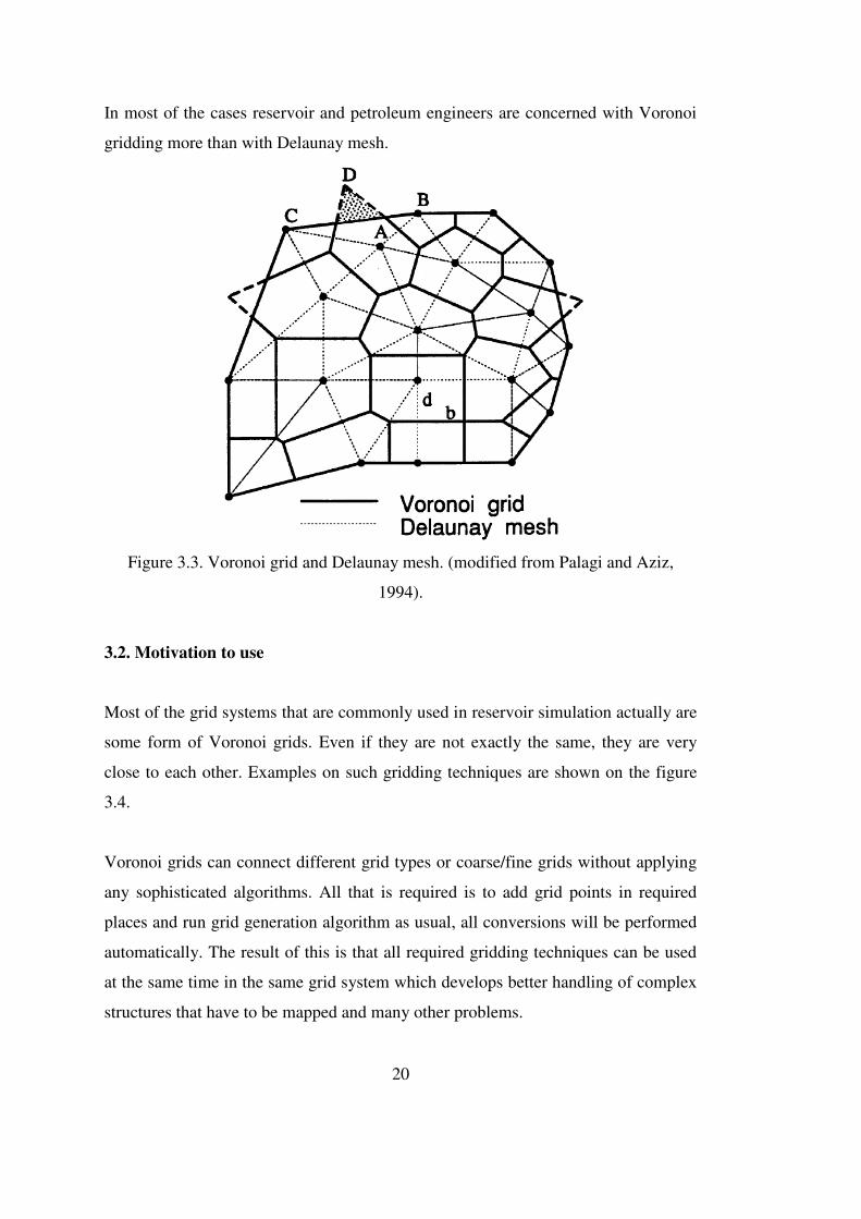
Voronoi grid consists of Voronoi grid block which are defined as the area around
grid point that is closer to this point than to any surrounding ones (Figure 3.3.).
Boundaries of grid blocks are perpendicular to the line connecting neighboring grid
points and intersect this line just in the center (that is why it is also called
perpendicular bisection). The latter means that Voronoi grid can be associated with
point-distributed type of grids.
On the figure 3.3, dashed lines that are connecting neighboring grid points are called
Delaunay mesh which consists only of triangles. If the line exists, it means that flow
can occur between the points that are connected. Actually, Delaunay mesh can
consist not only of triangles, but also of lines, rectangles and higher order polygons.
20
In most of the cases reservoir and petroleum engineers are concerned with Voronoi
gridding more than with Delaunay mesh.
Figure 3.3. Voronoi grid and Delaunay mesh. (modified from Palagi and Aziz,
1994).
3.2. Motivation to use
Most of the grid systems that are commonly used in reservoir simulation actually are
some form of Voronoi grids. Even if they are not exactly the same, they are very
close to each other. Examples on such gridding techniques are shown on the figure
3.4.
Voronoi grids can connect different grid types or coarse/fine grids without applying
any sophisticated algorithms. All that is required is to add grid points in required
places and run grid generation algorithm as usual, all conversions will be performed
automatically. The result of this is that all required gridding techniques can be used
at the same time in the same grid system which develops better handling of complex
structures that have to be mapped and many other problems.

21
Voronoi grid can also be used for simulating three-dimensional reservoirs. In this
case, usually Voronoi grid is created in the same conventional way for each of the
layers one by one.
Figure 3.4. Common grid techniques that can be associated with Voronoi (modified
from Palagi and Aziz, 1994).
3.3. Voronoi grid generation algorithm
There are many different grid generation algorithms. They are discussed in many
literature sources, such as paper by Ho-Le (Ho-Le, 1988). In this thesis, only one
grid generation algorithm will be presented in order to provide some information
how it occurs. The algorithm described here was created by Frederick et al
(Frederick et al., 1970).
This algorithm requires two inputs. One is the set of grid points of the blocks that
will be generated, and the other one is rmax - the maximum radius. This rmax is used in

22
characterization of outer boundary. If rmax is a large number, outer boundary of each
block will be convex, if not, then it may be concave in some regions. Also, it must be
said that the user of this algorithm is not required to explicitly identify grid points on
the boundary of the region that will be divided into blocks. For more detailed
discussion Palagi work (Palagi, 1992) can be referred to.
1. Choose a grid point (m).
2. Get the points that may become neighbors (n) in such a way, that the spacing
between (n) and (m) would be less than the value of rmax multiplied by two
(Lij<2*rmax). After all these points are selected, all other points are stopped to
be considered during the next stages.
3. Choose the point on the closest distance from the grid point (m) (minimal
Lmn).
4. Now you have line (mn). Find the next grid point (o) moving in counter-
clockwise direction, so that môn would be maximal.
5. Next step is to generate a circle that all three points lay on and calculate
radius of it. This radius is then named as rc. Now the first vertex of Voronoi
grid block with center (grid point) in (m) can be found as the center of the
circle. This vertice may fall outside of the area that will be divided into
blocks (e.g. point D in figure 2.3).
6. Then there are two cases: if rc < rmax, (o) is really a neighbor of block (m).
Then you must set (n)=(o) and redo stages four and five. After some time the
new neighbor is the first one, which means that all neighboring points have
been processed. If this is the case, then grid block (m) is totally inside of the
domain, and the other point for generation should be selected. Then
everything is done from the beginning. This procedure should be performed
for all points.
7. The second case is rc > rmax. This means that grid block intersects the outer
boundary of the domain. If this is the case, continue with the next step.
8. Make (n) equal to the first grid point as in the third step. Perform stages four
to seven in the clockwise direction till you reach another point outside of the
domain. Then start from the beginning with the new point and continue while
all the grid points are not processed.
23
9. After stages one to eight have been implemented for each of the points, the
next step is to calculate all angles between points on the border of the domain
and the corresponding grid points, such as angle CÂB on figure 3.3.
10. Then there are two cases. Both of them will be discussed on an example of
CÂB. If this angle is less than π/2, then central point of BC is a vertex of the
grid block that contains points B and C.
11. Otherwise, if this angle is bigger than π/2, then some part of the grid block
must be out of the domain and therefore must be deleted. After this outside
part is deleted, neighboring blocks also should be adjusted.
12. And the last step is to delete all the lines that have width less than some
predefined small number
(Palagi, C. L. and Aziz, K. Appendix (1994))
As it was said before, there are many other Voronoi grid generation algorithms that
can be found in literature. Some of them are: Fortune's algorithm (or sweep line
algorithm), Lloyd's algorithm, Bowyer-Watson algorithm etc. In this study Voronoi
generation was used only for visualization of results. This visualization was
performed by use of Matlab software using "Voronoi" function.
3.4. Use of Voronoi grid in reservoir simulation
As it was mentioned, use of Voronoi grids in reservoir simulation was firstly
described in 1989 by Heinemann and Brand. After this introduction many scientists
and engineers started to explore newly discovered horizons, perfect what was
already done and tried to find additional use to them. This subchapter provides some
information on how Voronoi grids were used in petroleum industry during last 26
years.
In the first years of usage of Voronoi grids one of the most productive unions was
duet of Cesar Luiz Palagi and Khalid Aziz in Stanford university. In 1992 Palagi
graduates from Stanford University and publishes his PhD dissertation called
"Generation and application of Voronoi grid to model flow in heterogeneous
24
reservoirs" (Palagi, 1992). His supervisor on this work was Khalid Aziz. After
graduation they publish together several more papers related to Voronoi gridding in
reservoir simulation (Palagi and Aziz, 1993; Palagi et al., 1993; Palagi and Aziz,
1994). Most of these papes concentrate on general application of Voronoi to
reservoir simulation, but some of them also discuss proper handling of horizontal
and vertical wells using Voronoi grids.
After usage of Voronoi gridding technique in reservoir simulation proved to be
efficient, several authors tried to create commercial black oil simulators that will use
Voronoi grid in order to model reservoir behavior. Such type of model is discussed
in the paper of Kuwauchi et al. (Kuwauchi et al., 1996). In this paper results obtained
from the simulator using Voronoi grids are compared with analytical solutions and
decision on effectiveness of reservoir simulator with Voronoi grids is made.
In the XXI century applications of Voronoi grid in reservoir simulation increase with
more and more different applications. Some authors provide information on
geological models' upscaling techniques with Voronoi (Prevost et al., 2004; Branets
et al., 2009), others try to generate grid in such a way so that it would honor not only
geological strutures, but also flow of fluids in the reservoir (Castellini, 2001;
Mlachnik et al., 2006; Merland et al., 2011; Moog, 2013); some of the authors
propose new Voronoi generation algorithms (Evazi and Mahani, 2009; Katzmayr
and Ganzer, 2009), others provide techniques for better handling of wells and
fractures (Syihab, 2009; Li, 2011; Olorode, 2011; Fung et al., 2014).
Nowadays, Voronoi package can be found in some of the popular commercial
simulators, however, usage of Voronoi grid in the industry is still not very popular.
Among causes of this, Fung et al. (Fung et al., 2014) mentions extra stages that are
required in order to generate Voronoi mesh, difficulties in populating of properties
into Voronoi grid blocks and in the calculation of data related to well perforation.
Also he mentions that in further stages of reservoir simulation generation such as
history match, future predictions runs with different well locations etc. Voronoi grid
requires more sophisticated and therefore less attractive reservoir modeling tools,
which results in overall unattractiveness of the method. Another paper written by

25
Vestergaard et al. (Vestergaard et al., 2008) describes application of Voronoi grids to
the problem of modeling of giant carbonate reservoir. Among the complications that
they dealt with while building the model, problems with history match, inefficiency
of linear solvers which were less efficient than for the case of Cartesian grid with
similar grid block sizes are mentioned. Also it must be said, that before trying to
apply Voronoi gridding technique to this problem, Cartesian grid simulation was
performed, which was proved to be incompatible with the real data.
So, decision on whether to use or not Voronoi gridding technique in reservoir
simulation is still open.

26

27
CHAPTER 4
RESERVOIR HETEROGENEITIES AND ANISOTROPY
4.1. Introduction
From the petroleum engineering point of view, definition of term "reservoir
heterogeneity" would be geological intricacy of a reservoir and how this intricacy
affects flow of fluid. (Alpay, 1972) In simpler terms, it is "spatial changes of
reservoir properties in reservoir".
This complexity is usually a result of changes in strata that occur after deposition, for
example, under compaction, tectonic distortion and cementation. There are different
classifications of reservoir heterogeneities, but the most widely used are as follows:
microscopic heterogeneities (less than 1mm), mesoscopic heterogeneities (up to 1m),
macroscopic heterogeneities (tens of meters) and megascopic heterogeneities
(hundreds of meters) (figure 4.1)
Microscopic heterogeneities are heterogeneities on scale of pores and grains of
formation. Mesoscopic heterogeneities can be seen on vertical measurements, e.g.
during coring and logging. They alter such properties as permeability of matrix,
rock-fluid interaction, formation damage and directional fluid flow. They include
bedding, changes in lithology, and others.
Macroscopic heterogeneities occur on the interwell scale. They include faults,
pinchout, erosional cut-out and others. Macroscopic heterogeneities can be seen
during well tests or on seismic survey results. The show great effect on sweep
efficiency, patterns of flow, profitability of secondary recovery and EOR.

28
Megascopic are the biggest possible reservoir heterogeneities. They occur on a
fieldwide scale. They are related to depositional environment and the structure of the
field. Usually megascopic heterogeneities affect petroleum reservoir volumetrics,
and therefore petroleum production trends.
Figure 4.1. Reservoir heterogeneity classes (modified from Weber, 1986).
This study faces up with one type of reservoir heterogeneity that will be discussed
further in the chapter - channeling.
4.2. Channeling
Channeling is found usually in fluvial deposit systems. This means that during some
time in the history here existed flowing body of water, e.g. river. Actually, there are
two types of fluvial deposit systems: braided and meandering fluvial systems.

29
Braided fluvial pattern usually occurs when the river does not have enough discharge
to take its sediment load with itself or in the cases when the river has banks that can
be easily eroded. In most of the cases braided pattern can be found in the upper parts
of a fluvial deposit system. In those regions bodies of water usually have steeper
gradients, mainly coarse sediments and frequent changes in discharge. These
conditions result in frequent intersection of channels, as it can be seen on figure 4.2.
So, this means that the channel that is created in result is a very complicated system
consisting of great amount of frequently intersecting channels.
Figure 4.2. Braided fluvial deposition system (modified from Galloway and Hobday,
1996).
As it was already said, frequent discharge changes result in overloading of sediment.
During flood, body of water is able to move all of its sediments. Nevertheless,
usually rivers have little amount of flowing water, which results in inability to move
sediments by flow. Because in the upper parts of fluvial deposit system coarse
sediments are usually deposited, base of the resulting channel consists of coarse
particles, which means better reservoir qualities in the future (if this structure is not
affected greatly by the post-depositional conditions).

30
Meandering fluvial pattern (Figure 4.3) occurs in lower parts of fluvial deposition
system. This is due to more gently sloping gradient than in the braided systems. The
closer braided systems are to the source of the river, the straighter they are; the
farther they are from the source, the more meandering character they get, until fully
meandering system is not created. Here, flow has less speed, higher depth, which
results in the fact that stream becomes affected by centrifugal force and bends
towards the external bank. Because of this, external bank becomes severely eroded,
the river is able to move towards this bank deeper in lateral direction. Therefore, the
river itself becomes more and more tortuous until these sides of the river are not
separated from each other by a thin layer of formations. After some time this layer is
also eroded, and now the river has a better, straighter way to move, leaving one of its
flanks behind. These left flanks are then called cutoffs.
Figure 4.3. Meandering fluvial deposition system (modified from Prothero and
Schwab, 2014).
Sediments accumulated here are mainly on the inner sides of the river. As in the
braided fluvial deposition system, sediments closer to the source are coarser ones,
while towards the end they become finer. (Prothero and Schwab, 2014)
These effects result in heterogeneities called "channeling" in reservoirs. In these
channels property values may differ from the same properties of the part of reservoir

31
not affected by this channel. This is one of the cases, that was considered during this
study.
4.3. Anisotropy
A formation is called anisotropic if the value of property in one direction differs
from the value of the same property in another one. Most usual earth anisotropy is
between vertical on horizontal directions, called transverse anisotropy, but it is not
considered in this study. This study tries to deal with anisotropy of directional
permeabilities in the horizontal plane, thus permeability in x-direction differs from
permeability in y-direction. Before going further, this chapter will explain where
anisotropy comes from and why it is different from reservoir heterogeneities.
As it was already mentioned, anisotropy is not the same as heterogeneities discussed
previously in the chapter, however, they are usually confused with each other. There
are two main differences between them.
The first one is that in anisotropy changes of reservoir properties occur at one point,
but in a different direction (vector value), while heterogeneity means that there are
differences in scalar or vector values in two or more different points. The second
difference is that anisotropy deals mainly with physical properties, while
heterogeneities may deal with anything starting from the same physical properties
and ending with the composition of formation.
Anisotropy results from processes occurring during and after deposition. For
example, anisotropic changes in carbonates, such as changes in directional
permeabilities, may be a result of layering which affects carbonate mineralogy by
changing formation diagenetic potential and texture. As opposed to carbonates, in
the clastic rocks anisotropy can occur only if the rock is homogeneous or uniform to
some extent. If the formation is totally heterogeneous, then no anisotropy can occur
there, because in this case there will not be any directionality in the rock. Summing
this up we may come up with a conclusion that anisotropy developing with the

32
deposition has two causes: periodic layering and grains ordering, which results from
the directionality of the rock. (Rajan, 1988). This ordering is mainly performed by
gravitational forces and transport.
Figure 4.4. Example on diagenetic changes (Anderson et al., 1994).
After deposition, formation undergo changes due to diagenesis. Diagenesis is
exposion of formation to different forces of chemical, physical and biological
character after deposition. During this stage many changes can occur in formation
structure: for example, when formation is buried at increasing depth, the overburden
pressure increases with depth and may cause rearrangement or rotation of grains in
the horizontal plane (Manrique et al., 1994). Other factors that may affect formation
properties in the horizontal plane are fractures or plastic deformation and many
others.
For understanding of anisotropy, processes occurring during diagenesis should be
always considered, because they can dramatically change the properties of the
formation, even properties already changed during deposition. For instance,
alterations in ordering/packing and horizontal orientation (this also affects formation
permeability) that took place during deposition may be totally demolished by the
diagnetic processes.
On figure 4.4 depositional anisotropy is absolutely changed by the clay and quartz
overgrowth. The point of this example is that permeability model should be based on
both depositional and diagenetic alterations of rock, otherwise the representation of

33
formation will be incorrect, which can affect all following calculations. (Anderson et
al., 1994)
This study shows attempt to carefully divide reservoir, including heterogeneity and
anisotropy into Voronoi blocks in order to produce a representative result using
limited amount of grid blocks.

34

35
CHAPTER 5
OPTIMIZATION
5.1. Introduction to optimization
Optimization, as a tool helping to solve different kind of problems, was
accompanying humankind from the very beginning of its existence. Actually, at first
this kind of optimization was absolutely primitive and was based on the instincts of
early humans: they waited for most optimum conditions to plant or harvest crops,
decided on whether to start a war with another tribe or used optimization when
hunting animals - how many men are required to track down an animal and to kill it
in as safe manner as possible.
With the introduction and development of mathematical methods, optimization
methods also underwent an advancement, but still were quite primitive. The greatest
advancement of optimization techniques took place in last fifty-sixty years with the
development of computational technologies. After that, optimization methods had
dramatic improvement that is still continuing nowadays. While optimization
algorithms were developing at an enormous rate, the technologies required for
implementation of this algorithm were also advancing. This created ideal conditions
for optimization, and now it is difficult to imagine complex and even usual projects
in various disciplines that would not use any kind of its form (Diwekar, 2008).
Optimization is the process of choosing the 'best' out of all solutions of the problem,
if the "good" can be separated from the "bad" and measured. In our day-to-day life,
everyone would like to have the "maximum" in some good things, like salary, health
or holidays or "minimum" in bad things as expenses, over-time work and problems.

36
Taking this into account, the term "optimum" may be described as the "minimum" or
"maximum" depending on the conditions, for example maximizing the salary while
minimizing the over-time work. So the word "optimum" is much more useful than
the term "best" in the same way as the term "optimize" is a way better than the word
"improve". So, theory of optimization is a section of mathematics dealing with the
study of optimum solutions of the problems and the procedures to obtain them.
As it was said before, the optimization is used in a wide range of various disciplines
including math, physics, business and economics, social sciences, engineering and
even politics. It covers all engineering disciplines, starting from chemical and
petroleum engineering and ending with mechanical and electrical engineering. Most
common engineering areas of usage of optimization algorithms include design of
buildings, creation of tools, curve fitting, modeling of systems and many others.
Almost all real optimization problems do not have only one solution. Actually,
amount of solutions may be up to infinite. That is why optimization based on some
of the criteria that govern the behavior of the solutions is so important. (Antoniou
and Lu, 2007)
5.2. Classes of optimization algorithms
An algorithm is a collection of actions that should be performed in order to solve
some problem. They are usually written with human language, not with computer
code, so it would be easy to understand for humans and would not depend on the
programming environment or specific computers. Optimization algorithm is an
algorithm of the type described in the previous sentence, that can be used to get
optimum solutions of optimization problems.
There are two broad groups of optimization algorithms: deterministic and
probabilistic.

37
Figure 5.1. Rough classification of optimization algorithms (modified from Weise, 2011).

38
Further subdivision is quite a difficult job, because some of the algorithm classes
take properties of both basic classes, but some rough estimation is shown on the
figure 5.1.
Deterministic optimization algorithms are algorithms that during each step have only
one way to move to the next one. This means that if the same set of data is used as
input, this algorithm will do absolutely the same thing and the results will also be the
same. So, this type of optimization algorithms is mostly suitable for the cases when
the most efficient decisions on how to proceed in different situations are known and
used in the algorithm. These cases occur when the dependence between the different
properties of the probable solutions of the problem and their utilities are clearly
understood and used.
In some cases the manner of how the deterministic algorithms approach the problem,
may cause problems in getting the most optimal solution. This is the situation when
the dependence between the solution and the goodness of it is not so straightforward
(for example, changing or very complex), or when the size of the search space is
enormous. In such kind of cases application of deterministic algorithms is not very
efficient and the use of probabilistic ones is much more effective choice.
Deterministic algorithms include search algorithms, which are subdivided into
informed (including Gready and A* searches) and uninformed search (including
Breadth-First search (BFS), Depth-First search (DFS), and Iteratively Deepening
Depth-First Search (IDDFS)).
As opposed to deterministic optimization algorithms, probabilistic ones have
minimum one step in it that is based on the generation of random numbers. This
means that the approach will generate random solutions, which is a very useful step
if you do not know exactly how to proceed. These random approach, of course, has
disadvantages - for example, if the set of input data is the same, algorithm still will
produce different results, and still in many cases, they are preferable. Probabilistic
optimization algorithms include metaheuristics which is further subdivided into
evolutionary computation algorithms and algorithms that are not referred to that
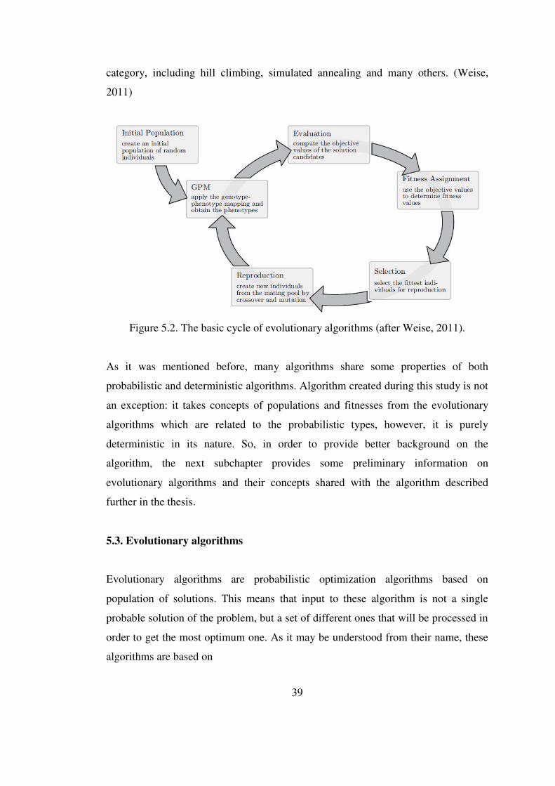
39
category, including hill climbing, simulated annealing and many others. (Weise,
2011)
Figure 5.2. The basic cycle of evolutionary algorithms (after Weise, 2011).
As it was mentioned before, many algorithms share some properties of both
probabilistic and deterministic algorithms. Algorithm created during this study is not
an exception: it takes concepts of populations and fitnesses from the evolutionary
algorithms which are related to the probabilistic types, however, it is purely
deterministic in its nature. So, in order to provide better background on the
algorithm, the next subchapter provides some preliminary information on
evolutionary algorithms and their concepts shared with the algorithm described
further in the thesis.
5.3. Evolutionary algorithms
Evolutionary algorithms are probabilistic optimization algorithms based on
population of solutions. This means that input to these algorithm is not a single
probable solution of the problem, but a set of different ones that will be processed in
order to get the most optimum one. As it may be understood from their name, these
algorithms are based on

40
analogy with some natural processes and mechanisms, such as biological evolution
and survival of the fittest conceptions. These algorithms use these ideas in the
processing of the population of solutions, hoping to find the one that is most suitable
for the problem under consideration.
Evolutionary algorithms were not developed together by one man. Actually, they
include a large set of different algorithms that were created to some extent by
different scientists and researchers. Evolutionary algorithms showed high flexibility
and performance in a wide range of different disciplines.
Despite that majority of evolutionary algorithms were invented by different
scientists, all of them undergo similar steps when initiated. These repeating steps are
called the basic cycle of evolutionary algorithms (figure 5.2). Following are the
stages of this cycle for evolutionary algorithm optimization with a single objective:
1. Population of probable solutions is used as an input to the algorithm. This
will be the first generation of solutions (t=1). This population may be random
or seeded, depending on the person who uses the algorithm and the problem.
If the initial population is seeded, this means that the used solutions are
already preprocessed and adapted to some extent to the criterion that is used
for optimization. It can even be the case when the whole first population
consists of such preprocessed individuals. These adapted solutions can be
obtained by using the same algorithm or by any other method. Seeding is
used to reach the optimum solution in a less number of generations. The
drawback of using seeding is that the fake convergence may be reached
before the actual convergence is achieved. This may be the result because
good solutions (or preprocessed) will have better fitness and will wipe out the
random solutions. So, this type of behavior must be considered before
applying of seeding.
2. Next step is to calculate objective functions for each individual solution in
the population.

41
3. Using values obtained from the previous step, distribute the values of fitness
to each of the individuals.
4. The next step is selection process - choosing individuals with higher fitness
values for reproduction, therefore wiping out individuals with lower
fitnesses.
5. The next step is reproduction - getting offspring from the parents selected in
the previous stage. This is done by applying of specialized reproduction
operations to the genotypes of the parents. Genotypes are just sets of genes.
They are usually obtained by converting solutions into binary, however, there
are also many other methods. Each "0" or "1" value inside of these genomes
are referred to as genes. This conversion is done for easier application of
reproduction operators. Most common reproduction operations are crossover
and mutation. Crossover is used to combine genotypes of parents together to
get genotype of children and mutation just makes changes in one genotype in
order to support diversity in the solutions. After reproduction is performed,
part of the last generation or the whole previous generation is swapped with
the children, depending on the choice of the person using the algorithm. This
will be the new generation. Number of generations is increased by one.
6. If the termination criterion is achieved, then everything stops here and
solution with the highest fitness is selected as the best one. If not, then
convert genotypes to phenotypes (this means converting of solutions into the
form, which is better suitable for calculation of objective functions. For
example, if the solutions are given in binary, convert them into system
suitable for calculation, which is usually decimal), then return to step 2 and
redo all the same thing for the new generations (Weise, 2011).
Now, after evolutionary algorithms were described, the last question that must be
answered is why exactly algorithm created in this study is based on evolutionary
optimization, but not on the other type of algorithms. The answer would be that the
algorithm of the solution to the problem that will be described in the "Methodology"
chapter is an iterative process, that uses population of solutions, trying to improve
population's worst performing individual solutions. Actually, that is what

42
evolutionary optimization algorithms are all about - they are highly suitable for such
kind of problems. However, the random part had to be eliminated from the process
and also the process of improvement of bad solutions was changed, making the
overall process deterministic, because exact direction of improvement is known from
the beginning, therefore, no randomification was required.
Algorithm created during this study uses population and fitness criteria described in
this chapter. More information on how exactly algorithm proceeds can be found in
"Methodology" chapter in this thesis work.

43
CHAPTER 6
PROBLEM STATEMENT
The aim of this study is to find an algorithm that will divide the reservoir model into
unstructured Voronoi grid blocks by considering the direction of permeability
vectors, anisotropy ratio, permeability or porosity heterogeneity of the reservoir in
such way that the defined error value in each block would be minimal. Voronoi grids
are strongly connected with the locations of grid points, that is why, by adjusting the
coordinates of grid points, shapes and locations of grid blocks can be altered, thus,
attempt to minimize the total error can be made. Since the main pressure gradients
exist around the wells, the representation of the wells is achieved by using closely
placed Voronoi grids around the wells as well.
This thesis provides detailed information on algorithm created for solving of the
problem described here and then shows some examples on how exactly it works.

44
45
CHAPTER 7
METHODOLOGY
7.1. Introduction
Algorithm created in this study is deterministic. As it was said before, this means
that for the same input values, the results produced by the algorithm will also be the
same. This algorithm consists of three major steps:
1. Generation of uniformly distributed grid points, taking into account
anisotropy in the reservoir;
2. Moving of grid points that have bad locations described by fitness values
(this deals with the effects of reservoir heterogeneity);
3. Adding of grid points related to vertical and horizontal wells or faults.
This chapter will cover these steps one-by-one.
Code of the algorithm written for Matlab can be found in Appendix A. Before
running of the algorithm, four column vectors called permXvec, permYvec,
permZvec (accordingly x, y and z coordinates of the points of petrophysical field)
and permeabilitiesVec (values of petrophysical property in the locations of points
assigned by vectors permXvec, permYvec and permZvec) should already be loaded
into the workspace. As it was mentioned before this petrophysical property field
should consist of densely and uniformly populated points with property values. For
creation of the field some extrapolation/interpolation methods may be required.

46
7.2. Step One (generation of initial population of grid points)
As it was previously mentioned, the first step consists in the generation of uniformly
distributed grid points throughout the reservoir. This distribution is created regarding
directional permeability relations in the reservoir. The first step requires several
input parameters: desired number of grid points (grid blocks); how many times
permeability in the y-direction is higher (or less) than the permeability in x-direction,
Ky/Kx (permeability in y-direction (Ky) divided by permeability in x-direction (Kx)
- these directions may not align with x- and y-directions of the reservoir); angle
between permeability in y-direction and y-direction of the reservoir (figure 7.1);
coordinates of vertices of reservoir; some small distance and small increment that
will be added to this distance at the end of each iteration.
Figure 7.1. Angle between permeability in y-direction and y-direction of the
reservoir.
Figure 7.2 shows an example on how the first step algorithm proceeds. The first
thing that the algorithm does - it finds coordinates of the starting point (red dot at
figure 7.2). If angle θ is between 0⁰ and 90⁰, then it calculates red dot coordinates
from: = − ∗ sin θ ∗ cos � (7.1) = ∗ sin θ ∗ sin � (7.2),
where startX - x-coordinate of starting point; startY - y-coordinate of starting point;
b - reservoir width. Minus sign is used in equation (7.1), because the lower left
corner of the reservoir is considered as (0;0) point, which means that starting point
will have negative x-coordinate.

47
If angle θ is between 90⁰ and 180⁰ (or 180⁰ and 270⁰, or between 270⁰ and 360⁰),
then 90⁰ (or 180⁰, or 270⁰) is subtracted from this angle and then formulas (7.1) and
(7.2) can be used. If angle θ is equal to 0⁰, 90⁰, 180⁰, 270⁰ or 360⁰, then lower left
corner of the reservoir (0;0) is chosen as the starting point. After starting point is
selected, the next step is to generate grid points.
Figure 7.2. First step example. Black rectangle - reservoir; green rectangle - area,
where grid points will be generated; red dot - starting point; a - reservoir length; b -
reservoir width.
The main idea behind this generation is that if permeability is higher in one direction
(x or y), then generated points need to be placed more densely in that direction - in
other words distance from one point to the next one in the permeability y-direction
divided by distance from the same point to the next one in permeability x-direction
should be equal to Ky divided by Kx.
So, for example, if permeability Ky is twice as Kx, then distance between points in
Kx direction is twice the distance between points in Ky direction.

48
Figure 7.3. Flowchart of step one.

49
This is because if permeability is higher in one direction than it is in the other, then
pressure disturbance generated by producing/injecting wells, when the simulation
will run, will propagate at a higher rate in the direction of higher permeability.
So, in order to accurately see how much this disturbance moves, grid points should
be placed more densely in that direction.
Because we know only relation of the distance in one direction to the distance in the
other one, but not exact values, we need to take some random small distance for one
direction and calculate distance in the other, so that we could generate these grid
points - that is what small distance in the input is used for. So, the algorithm starts to
generate points from starting point in Ky and Kx directions according to Ky and Kx
values and the small distance from the input. As it can be seen, some of the
generated points will fall outside of the reservoir (black rectangle), so after all of the
points are generated these points outside of the reservoir are ignored, while all the
points inside reservoir are counted. If the resulting number of grid points is higher
than the desired number of points entered as an input, then small distance is
increased by increment also entered as an input, then process starts from the
beginning with these new distances. This process is done until the number of grid
points is not less than the desired number. If distance in the beginning and increment
are not very large, resulting number of blocks should be very close to desired
number.
After the required number of grid points is achieved, the algorithm proceeds to the
second step. For better understanding, step one flowchart is shown on figure 7.3.
7.3. Step Two (movement of the bad grid points)
After all the grid points were generated, the next step is to check if their placement is
good enough. If it is bad, it would be better to move them to better places. This step
also requires some input values, namely: field of petrophysical property that will be
used to define different regions of the reservoir, number of iterations, number of
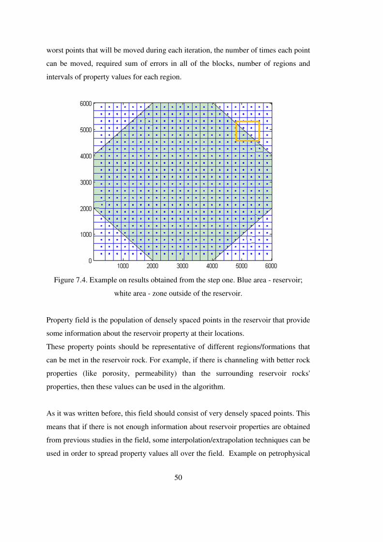
50
worst points that will be moved during each iteration, the number of times each point
can be moved, required sum of errors in all of the blocks, number of regions and
intervals of property values for each region.
Figure 7.4. Example on results obtained from the step one. Blue area - reservoir;
white area - zone outside of the reservoir.
Property field is the population of densely spaced points in the reservoir that provide
some information about the reservoir property at their locations.
These property points should be representative of different regions/formations that
can be met in the reservoir rock. For example, if there is channeling with better rock
properties (like porosity, permeability) than the surrounding reservoir rocks'
properties, then these values can be used in the algorithm.
As it was written before, this field should consist of very densely spaced points. This
means that if there is not enough information about reservoir properties are obtained
from previous studies in the field, some interpolation/extrapolation techniques can be
used in order to spread property values all over the field. Example on petrophysical

51
field consisting of 56400 permeability points for the field shown on figure 7.4 is
shown on figure 7.5.
Figure 7.5. Example on petrophysical field.
It must be mentioned that this property field should also include points outside of
reservoir with zero values, so that algorithm would understand where the boundaries
of reservoir are located.
Imagine, that the reservoir, that has to be modeled, is not of rectangular shape (or has
heterogeneities (such as channeling, etc.)). The first step has already been
implemented, resulting in a scheme shown on figure 7.4. Input values for the first
step were: 500 grid points, octagonal reservoir, no anisotropy or heterogeneities,
angle is equal to zero. Because each grid block can only have one property value
calculated as the average of all property points that fall inside of this block,
gridblocks on the edges of the reservoir (or on the edges of heterogeneities if they
are present) will not be representative of the area they cover.

52
Figure 7.6. Flowchart of step two.
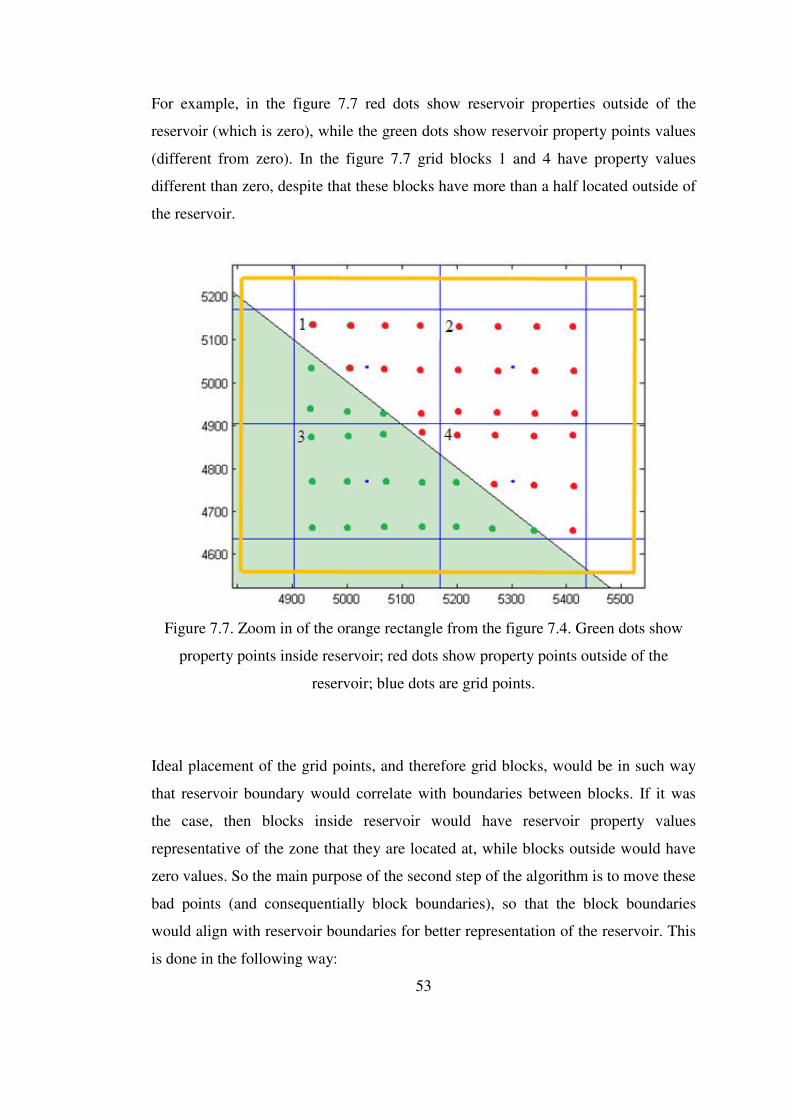
53
For example, in the figure 7.7 red dots show reservoir properties outside of the
reservoir (which is zero), while the green dots show reservoir property points values
(different from zero). In the figure 7.7 grid blocks 1 and 4 have property values
different than zero, despite that these blocks have more than a half located outside of
the reservoir.
Figure 7.7. Zoom in of the orange rectangle from the figure 7.4. Green dots show
property points inside reservoir; red dots show property points outside of the
reservoir; blue dots are grid points.
Ideal placement of the grid points, and therefore grid blocks, would be in such way
that reservoir boundary would correlate with boundaries between blocks. If it was
the case, then blocks inside reservoir would have reservoir property values
representative of the zone that they are located at, while blocks outside would have
zero values. So the main purpose of the second step of the algorithm is to move these
bad points (and consequentially block boundaries), so that the block boundaries
would align with reservoir boundaries for better representation of the reservoir. This
is done in the following way:
54
1. Calculate error and fitness values for each block. The error in the grid block
is equal to the standard deviation of reservoir property values that fall inside
of this grid block. For example, petrophysical field's points with permeability
values equal to 500, 510, 570 and 620 md fell inside one block. Two regions
of petrophysical fields were defined before: with permeabilities less than 550
md and with permeabilities higher than this values. Therefore, error of the
block is equal to standard deviation of these values, which is equal to 55.98.
This value is assigned to the block and is used in further calculations.
However, if the block is totally inside one region, then error is equal to zero.
The choice of standard deviation as an error left from very simple early runs
of the algorithm, when it was very effective. Because no better alternative
was found for the error function for more difficult late runs, it made its way
into the final version of the algorithm.
2. Each block is also assigned a fitness value, which is its rank (or place) in a
row of blocks' errors in a descending order.
3. Calculate sum of all error values.
4. For "n" (given as an input - number of points that will be moved during each
iteration) least fit grid points (highest error values) do the following
procedure: check if grid point can be moved at least once more; understand
where grid point is located; get property points inside this block; if the grid
point is inside one region, calculate mean values of the coordinates of all
other property points and move the grid block in the opposite direction from
the resulting mean property point at a distance given in the input.
5. Increase iteration counter by one.
6. If an iteration counter is less than a predefined number of required iterations,
return to step one, do all the steps again. If the iteration counter has reached
the predefined number of iterations, then take the result that has least sum of
errors and use it in the next step. This means that the best result in terms of
error function is chosen as an input for the next step. However, this best
result is the best only for the entered input parameters, by changing them
better or worse results may be achieved. This problem will be discussed in
the chapter 8.3, where effects of different input values are reviewed.
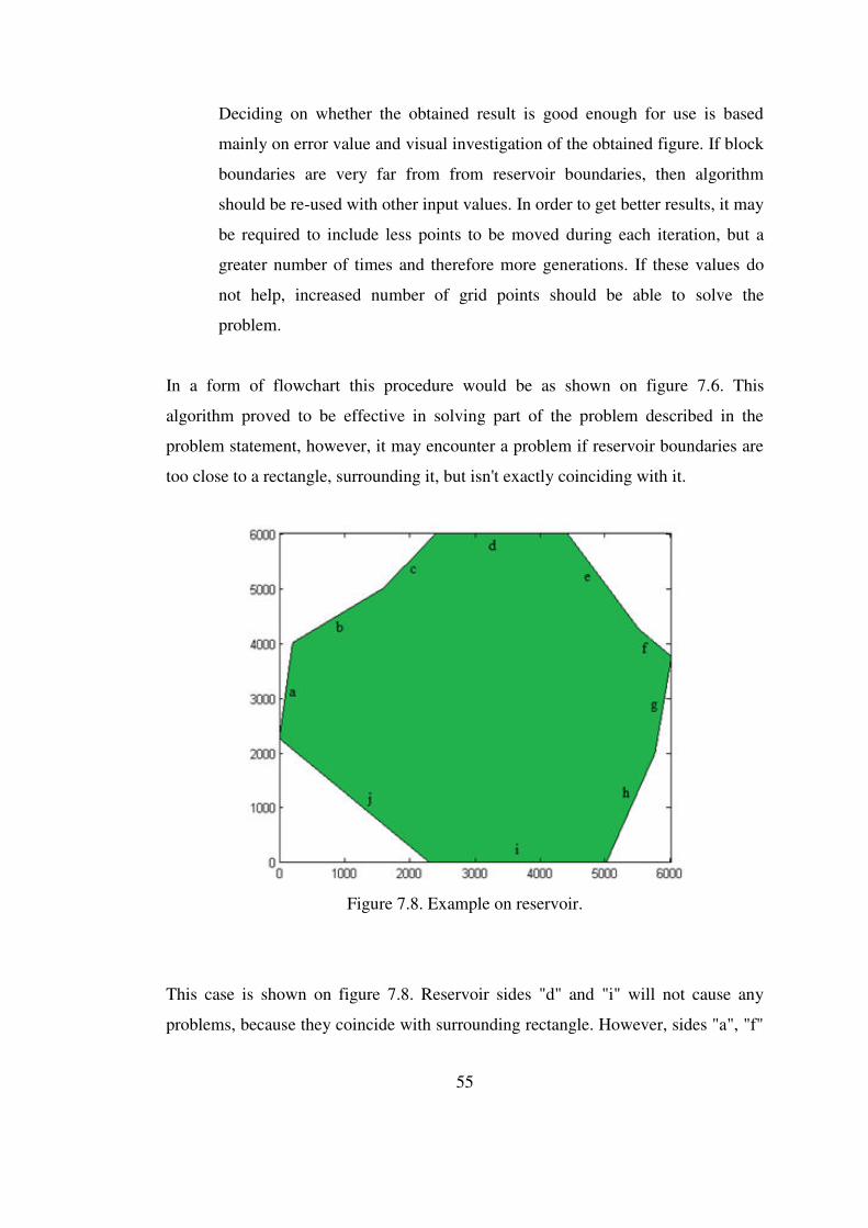
55
Deciding on whether the obtained result is good enough for use is based
mainly on error value and visual investigation of the obtained figure. If block
boundaries are very far from from reservoir boundaries, then algorithm
should be re-used with other input values. In order to get better results, it may
be required to include less points to be moved during each iteration, but a
greater number of times and therefore more generations. If these values do
not help, increased number of grid points should be able to solve the
problem.
In a form of flowchart this procedure would be as shown on figure 7.6. This
algorithm proved to be effective in solving part of the problem described in the
problem statement, however, it may encounter a problem if reservoir boundaries are
too close to a rectangle, surrounding it, but isn't exactly coinciding with it.
Figure 7.8. Example on reservoir.
This case is shown on figure 7.8. Reservoir sides "d" and "i" will not cause any
problems, because they coincide with surrounding rectangle. However, sides "a", "f"

56
and "g" may cause such problem, because they are very close to the vertical sides of
the rectangle.
If the distance from them to the rectangle sides is less than small distance obtained at
the end of step one, then the problem may occur, because points required outside of
the reservoir in order to generate block boundary coinciding with reservoir
boundary, may fall outside of black rectangle and therefore will not be generated.
Figure 7.9. Treating of vertical wells.
This problem is solved by adding of one layer of grid points on the different sides of
reservoir boundaries that have both starting and ending points closer to the rectangle
sides than small distance from the end of step one. This increases the resulting
number of grid blocks, but solves the problem effectively.
After handling of reservoir boundaries, points located inside rectangle but outside of
reservoir can be deleted. This is done by moving of all reservoir's vertices from the
center at a greater distance between the points multiplied by one and a half. Greater
distance is one of the distances (in Ky or Kx direction) obtained at the end of step
57
one. It is multiplied by 1.5 to make sure that at least one layer of points is left outside
of reservoir in order to handle all boundaries. So, reservoir vertices are pushed from
the center, area of reservoir increases in all of the directions. After this all points
outside of this big reservoir are deleted. These new bigger reservoir vertices are not
used after this step.
As it may be understood from the algorithm, the result will strongly depend on the
input parameters: how many points will be moved during each iteration; number of
required iterations; distance at which least fit points will be moved. For better
efficiency of the algorithm, it is proposed to use a greater number of iterations with
less points to be moved during each iteration at smaller distances but for a greater
number of times. However, usage of these characteristics means that calculation time
will increase, so the final decision on which values to use will depend on the person
using the algorithm.
After the best solution is chosen, the algorithm can proceed to the step 3, where grid
points related to vertical/horizontal wells and faults can be added.
7.4. Step Three (adding of grid points related to wells and faults)
Step three adds grid points related to vertical and horizontal wells and faults.
Vertical and horizontal wells are treated in different ways, while faults are treated
almost in the same way as horizontal well, so discussion is divided into two blocks -
vertical wells are discussed in one sub-chapter, horizontal wells and faults are
discussed in the other.
7.4.1. Treatment of vertical wells
Before talking about inputs for this step, it is required to show how the vertical wells
are treated. Figure 7.9 shows how grid points around vertical wells should be
generated.

58
Here, well is located in the middle of the structure, while surrounding blocks are
created in order to accurately represent a pressure drop in the area around the well.
These surrounding blocks are placed very densely, because the greatest pressure
drop occurs just around wells, so the more points are used there, the better
representation of the real conditions can be achieved.
Figure 7.10. Treating of horizontal wells.
As it may be seen from the figure 7.9, new blocks should be generated around the
well, and no grid points from the previous steps should interrupt their pattern. Also,
the number of blocks and layers, distances between layers of points and distance
from the well to the farthest layer of grid points should be considered. All these
values, along with the location of the well, its radius, should be entered as an input.
After these input values are entered, the algorithm starts by deleting grid point
generated during previous steps that fall into the region around well that will be
repopulated. After all these points are deleted, grid point related to the well is
generated, and then all surrounding points are generated layer-by-layer. This will end
up with something close to the pattern shown on figure 7.9.
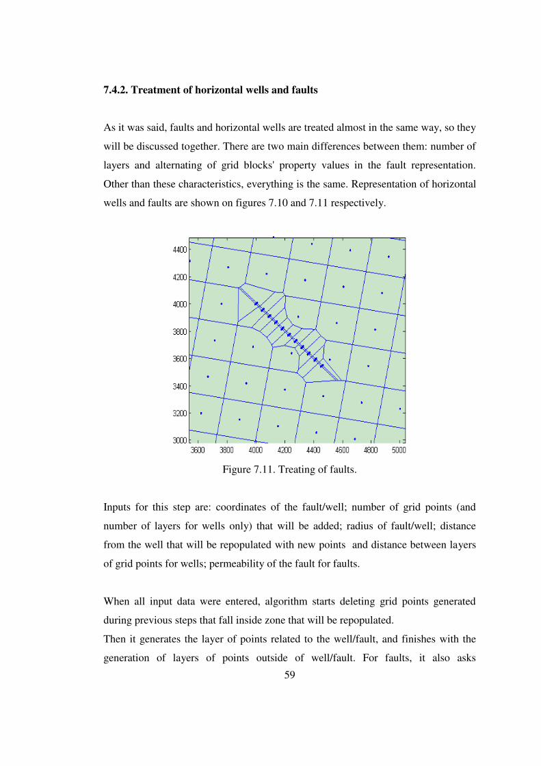
59
7.4.2. Treatment of horizontal wells and faults
As it was said, faults and horizontal wells are treated almost in the same way, so they
will be discussed together. There are two main differences between them: number of
layers and alternating of grid blocks' property values in the fault representation.
Other than these characteristics, everything is the same. Representation of horizontal
wells and faults are shown on figures 7.10 and 7.11 respectively.
Figure 7.11. Treating of faults.
Inputs for this step are: coordinates of the fault/well; number of grid points (and
number of layers for wells only) that will be added; radius of fault/well; distance
from the well that will be repopulated with new points and distance between layers
of grid points for wells; permeability of the fault for faults.
When all input data were entered, algorithm starts deleting grid points generated
during previous steps that fall inside zone that will be repopulated.
Then it generates the layer of points related to the well/fault, and finishes with the
generation of layers of points outside of well/fault. For faults, it also asks
60
permeability of the fault and then assigns entered value to the blocks that represent
this fault. After this procedure is finished, it asks if another well/fault will be added.
When all wells or faults are introduced, algorithm finishes its work by drawing
result.
It must be mentioned that the algorithm described here was used only in two-
dimensional problems. However, if there is a three-dimensional problem, the
algorithm can be run for each layer separately. Then all results may be gathered
together. If the layer is inclined and inclination angle is known, then layer can be
changed into horizontal position, where the algorithm can be run, and then results
can be converted back into inclined position. So, the algorithm is quite general and
can be used in many cases. As it was previously mentioned, the code for running this
algorithm was written in Matlab. This code can be found in Appendix A.
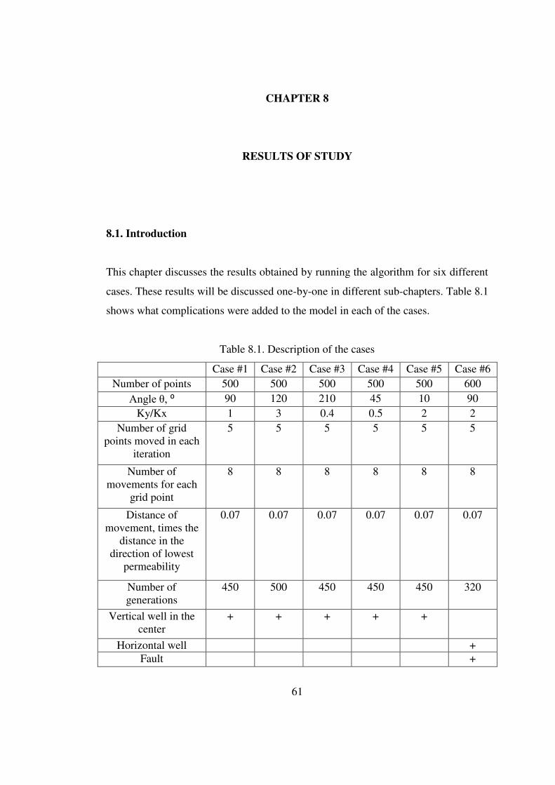
61
CHAPTER 8
RESULTS OF STUDY
8.1. Introduction
This chapter discusses the results obtained by running the algorithm for six different
cases. These results will be discussed one-by-one in different sub-chapters. Table 8.1
shows what complications were added to the model in each of the cases.
Table 8.1. Description of the cases
Case #1 Case #2 Case #3 Case #4 Case #5 Case #6 Number of points 500 500 500 500 500 600
Angle θ, ⁰ 90 120 210 45 10 90 Ky/Kx 1 3 0.4 0.5 2 2
Number of grid points moved in each
iteration
5 5 5 5 5 5
Number of movements for each
grid point
8 8 8 8 8 8
Distance of movement, times the
distance in the direction of lowest
permeability
0.07 0.07 0.07 0.07 0.07 0.07
Number of generations
450 500 450 450 450 320
Vertical well in the center
+ + + + +
Horizontal well + Fault +

62
This chapter describes results obtained after running of the six cases described in the
table and further in the chapter and makes conclusion if algorithm xreated for this
thesis work is effective or not.
Figure 8.1. Permeability field for cases #1, #2 and #6 (plotted using MATLAB).
8.2. Cases
8.2.1. Case One (no anisotropy, no heterogeneities, one vertical well).
This case is the most simple one. This case includes absolutely homogeneous,
isotropic reservoir with a vertical well in the middle. The reservoir is not rectangular.
Permeability field required for running of the algorithm is shown on figure 8.1.
All values are given in milli-darcies. This permeability field was generated randomly
in the required interval of permeability values. For all of the cases described in this

63
thesis, permeability field consists of 14400 uniformly distributed points - 120 rows
and columns.
Main inputs for the first step are as follows: 500 points; 90 degrees angle between
Ky and y-direction of the reservoir; no anisotropy or heterogeneities; small distance
equal to 5; increment in distance also equal to 5.
Figure 8.2. Results obtained after running of the first step for the case #1 (built in
MATLAB).
At the end of the first step resulting picture is as shown on figure 8.2. Resulting sum
of errors at this figure is equal to 18113. As it may be seen from the figure, grid after
the first step is a regular Cartesian grid or very close to it (in the other cases).
Main inputs for the second stage are: five worst points moved during each iteration;
eight movements for each point; 450 iterations; one region of permeabilities between
1 and 1000 md (entered as three column vectors - permX (x-coordinates of
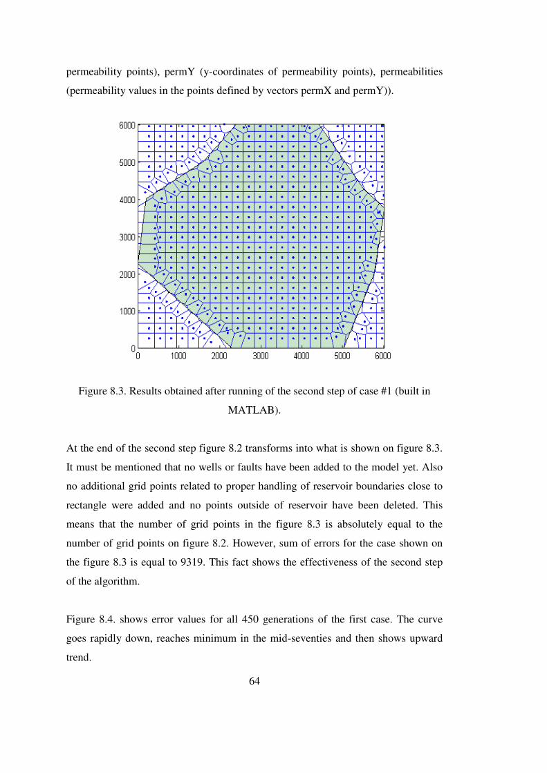
64
permeability points), permY (y-coordinates of permeability points), permeabilities
(permeability values in the points defined by vectors permX and permY)).
Figure 8.3. Results obtained after running of the second step of case #1 (built in
MATLAB).
At the end of the second step figure 8.2 transforms into what is shown on figure 8.3.
It must be mentioned that no wells or faults have been added to the model yet. Also
no additional grid points related to proper handling of reservoir boundaries close to
rectangle were added and no points outside of reservoir have been deleted. This
means that the number of grid points in the figure 8.3 is absolutely equal to the
number of grid points on figure 8.2. However, sum of errors for the case shown on
the figure 8.3 is equal to 9319. This fact shows the effectiveness of the second step
of the algorithm.
Figure 8.4. shows error values for all 450 generations of the first case. The curve
goes rapidly down, reaches minimum in the mid-seventies and then shows upward
trend.
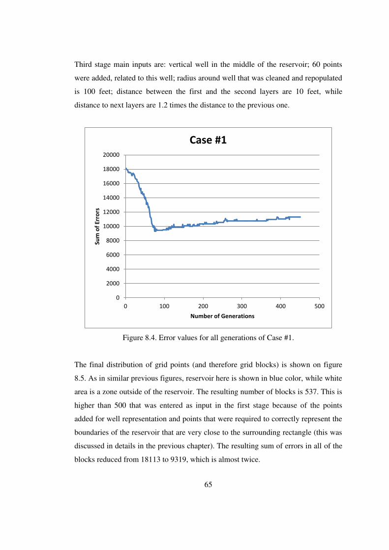
65
Third stage main inputs are: vertical well in the middle of the reservoir; 60 points
were added, related to this well; radius around well that was cleaned and repopulated
is 100 feet; distance between the first and the second layers are 10 feet, while
distance to next layers are 1.2 times the distance to the previous one.
Figure 8.4. Error values for all generations of Case #1.
The final distribution of grid points (and therefore grid blocks) is shown on figure
8.5. As in similar previous figures, reservoir here is shown in blue color, while white
area is a zone outside of the reservoir. The resulting number of blocks is 537. This is
higher than 500 that was entered as input in the first stage because of the points
added for well representation and points that were required to correctly represent the
boundaries of the reservoir that are very close to the surrounding rectangle (this was
discussed in details in the previous chapter). The resulting sum of errors in all of the
blocks reduced from 18113 to 9319, which is almost twice.
0
2000
4000
6000
8000
10000
12000
14000
16000
18000
20000
0 100 200 300 400 500
Su
m o
f E
rro
rs
Number of Generations
Case #1

66
After the dispensation of grid points shown on figure 8.3 was obtained, fluid flow
simulation was created. A Python code was written based on the flow equations
described in the book of Ertekin et al. (Ertekin et al., 2001) to make these
simulations.
Figure 8.5. Results obtained for the case #1 (built in MATLAB).
Inputs for this fluid flow simulation run are as follows: one vertical well in the center
producing 100 stb/d for 50 days with time step of 5 days. This means that data after
10 time steps was generated and analyzed. Initial reservoir pressure is equal to 3044
PSI, fluid is slightly compressible, only one phase present.
Expectations are to see pressure disturbance to propagate at the same speed in all
directions, because there is no permeability anisotropy and hetergeneities in the field.
This means that pressure disturbance propagation should take shape of a circle.
Compare with result shown on figures 8.6-8.15. As it may be seen, pressure
propagates at circular shape until it reaches reservoir boundaries.

67
Figure 8.6. Pressure distribution after 5 days.
Figure 8.7. Pressure distribution after 10 days.

68
Figure 8.8. Pressure distribution after 15 days.
Figure 8.9. Pressure distribution after 20 days.

69
Figure 8.10. Pressure distribution after 25 days.
Figure 8.11. Pressure distribution after 30 days.

70
Figure 8.12. Pressure distribution after 35 days.
Figure 8.13. Pressure distribution after 40 days.

71
Figure 8.14. Pressure distribution after 45 days.
Figure 8.15. Pressure distribution after 50 days.

72
8.2.2. Case Two (anisotropy, no heterogeneities, one vertical well).
This case is almost identical to the previous one, with the only exception: anisotropy
has been introduced. So, the reservoir is of irregular shape, with anisotropy but no
heterogeneities. One vertical well is introduced in the center. Permeability field is
the same as in the case #1. This means that it was also randomly generated in the
required intervals - between 1 and 1000 md.
Figure 8.16. Results obtained after running of the first step for the case #2 (built in
MATLAB).
Main inputs for the first step are as follows: 500 blocks; angle between Ky and y-
direction of the reservoir is equal to 120 degrees; permeability in y-direction is three
times higher than permeability in x-direction; small distance and increment are both
equal to 5 feet.
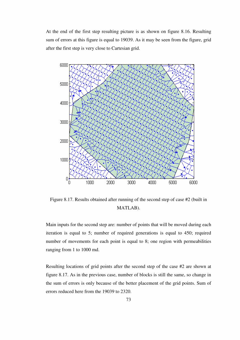
73
At the end of the first step resulting picture is as shown on figure 8.16. Resulting
sum of errors at this figure is equal to 19039. As it may be seen from the figure, grid
after the first step is very close to Cartesian grid.
Figure 8.17. Results obtained after running of the second step of case #2 (built in
MATLAB).
Main inputs for the second step are: number of points that will be moved during each
iteration is equal to 5; number of required generations is equal to 450; required
number of movements for each point is equal to 8; one region with permeabilities
ranging from 1 to 1000 md.
Resulting locations of grid points after the second step of the case #2 are shown at
figure 8.17. As in the previous case, number of blocks is still the same, so change in
the sum of errors is only because of the better placement of the grid points. Sum of
errors reduced here from the 19039 to 2320.

74
Figure 8.18. shows error values for all 500 generations of the second case. The curve
goes rapidly down, reaches minimum in the eighties and then shows upward trend.
Figure 8.18. Error values for all generations of Case #2.
Main inputs for the third stage are: one vertical well in the middle; radius around the
well that is cleaned and repopulated is equal to 100 feet; 60 points related to the well
are added; distance between the first and the second layer of points is equal to 10
feet, while distance to next layers are 1.2 times the distance to the previous one.
The resulting distribution of grid points (and therefore grid blocks) is shown on
figure 8.19. As in similar previous figures, reservoir here is shown in blue color,
while white area is a zone outside of the reservoir. The resulting number of blocks is
540. This is higher than 500 that was entered as input in the first stage because of the
points added for well representation and points that were required to correctly
represent the boundaries of the reservoir that are very close to the surrounding
rectangle (this was discussed in details in chapter 6).
0
2000
4000
6000
8000
10000
12000
14000
16000
18000
20000
0 100 200 300 400 500 600
Su
m o
f E
rro
rs
Number of Generations
Case #2

75
The resulting sum of errors in all of the blocks reduced from 19039 to 2320, which
means that sum of errors reduced more than eight times. The great effectiveness of
the algorithm for the second case, compared to the case number one, may be due to
input parameters entered in the step one - angle and anisotropy factor.
Figure 8.19. Results obtained for the case #2 (built in MATLAB).
It can also be seen from the figures 8.5 and 8.19. On the figure 8.19 block
boundaries are better aligned with reservoir shape than on the figure 8.5. From this,
the conclusion may be made that the algorithm's effectiveness depends on the
reservoir properties.

76
Figure 8.20. Velocity field combined with the contour map of the distribution of the
pressures after 5 days of production for the second case (obtained with Surfer).
Figure 8.21. Permeability field for case #3. Generated in MATLAB.

77
However, by adjusting the input parameters given in the second stage effectiveness
may be increased. For example, by minimizing the distance at which points are
moved in each iteration and by increasing the number of movements for each point
and number of iterations, slightly better results may be achieved. However, this
would require more computation time for the computer. So, the choice is totally on
the person using the algorithm.
For this case fluid flow simulation run was also implemented. All input parameters
are just the same as in the previous case: one vertical well in the center producing
100 stb/d for 50 days with time step of 5 days. Initial reservoir pressure is equal to
3044 PSI, fluid is slightly compressible, only one phase present.
Expectations are to see pressure disturbance propagate at higher rate in the north-east
and south-west directions because of the permeability anisotropy. This is what can
be seen on figure 8.20.
Other figures showing results of case #2 fluid flow simulation run are in Appendix
B.
8.2.3. Case Three (anisotropy, straight channel, one vertical well).
This is the first case where heterogeneity is introduced. This heterogeneity is
represented by a straight channel in the middle of the reservoir.
This channel has better permeability values than the surrounding reservoir - in the
channel permeability is between 500 and 1000 md, while in other parts of the
reservoir they are between 1 and 500 md. The algorithm should be able to handle not
only reservoir - outside of reservoir boundaries, but also reservoir - channel
boundaries. This is shown on figure 8.21 - representation of permeability field.

78
Figure 8.22. Results obtained after running of the first step for the case #3 (built in
MATLAB).
Figure 8.23. Results obtained after running of the second step of case #3 (built in
MATLAB).

79
Main inputs for the first step are as follows: 500 grid points; angle between Ky and
y-direction of the field is equal to 210 degrees; Ky to Kx relation is equal to 0.4;
small distance and each iteration increment are both equal to 5.
Figure 8.24. Error values for all generations of Case #3.
At the end of the first step resulting picture is as shown on figure 8.22. Resulting
sum of errors at this figure is equal to 19213. As it may be seen from the figure, grid
after the first step is very close to Cartesian grid.
Main inputs for the second step are: number of points that were changed during each
iteration is 5; 450 iterations; each point was allowed to move 8 times; as it was said,
the two regions were introduced: one with permeabilities between 1 and 500 md, the
other with permeabilities between 501 and 1000 md.
0
5000
10000
15000
20000
25000
0 100 200 300 400 500
Su
m o
f E
rro
rs
Number of Generations
Case #3

80
Resulting locations of grid points after the second step of the case #3 are shown at
figure 8.23. As in the previous cases, number of blocks is still the same as in figure
8.22, so change in the sum of errors is only because of the better placement of the
grid points. Sum of errors reduced here from the 19213 to 1821.
Figure 8.24. shows error values for all 450 generations of the third case. The curve
goes rapidly down, reaches minimum in the early one hudredth and then shows
upward trend.
Figure 8.25. Results obtained for the case #3 (built in MATLAB).
Main inputs for the third step are: one vertical well in the center of the reservoir;
radius around the well that was repopulated is equal to 100 feet; 60 points related to
this well was added; distance between the first and the second layers of points
around the well is equal to 10 feet; distance to the next layers are 1.2 times the
distance to the previous one.

81
Obtained result is shown on figure 8.25. The resulting number of blocks is 527,
while sum of errors in each block reduced from initial value of 19213 to the best
result of 2046, which is almost 10 times! This is even beyond expectations, because
it is even better than in the both previous, simpler cases.
Figure 8.26. Velocity field combined with the contour map of the distribution of the
pressures after 5 days of production for the third case (obtained with Surfer).
Why this happens is not very clear, but maybe this is due to the angle introduced in
the first step which somehow better coincides with reservoir boundaries and makes
the work of the algorithm easier. Increased number of blocks is still due to handling
of reservoir boundaries close to the outside borders and adding of grid points related
to the well.
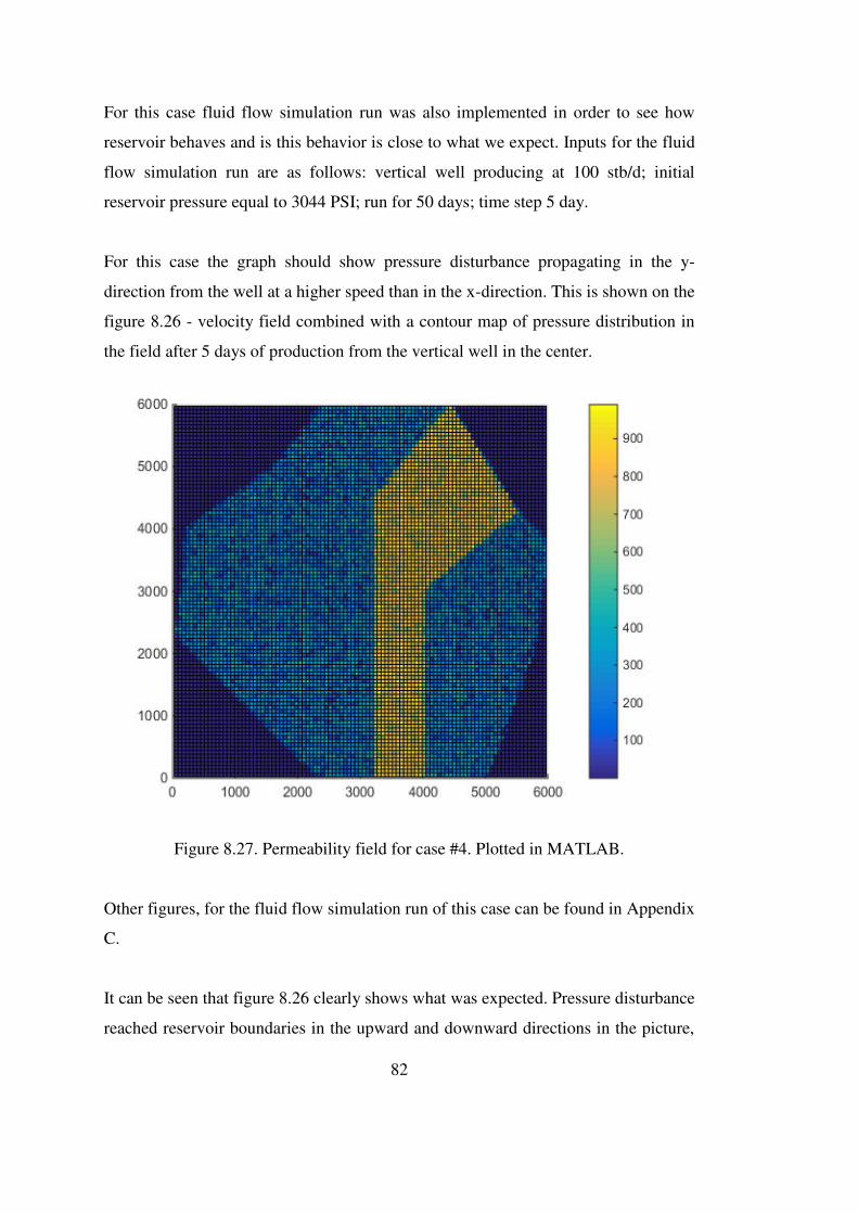
82
For this case fluid flow simulation run was also implemented in order to see how
reservoir behaves and is this behavior is close to what we expect. Inputs for the fluid
flow simulation run are as follows: vertical well producing at 100 stb/d; initial
reservoir pressure equal to 3044 PSI; run for 50 days; time step 5 day.
For this case the graph should show pressure disturbance propagating in the y-
direction from the well at a higher speed than in the x-direction. This is shown on the
figure 8.26 - velocity field combined with a contour map of pressure distribution in
the field after 5 days of production from the vertical well in the center.
Figure 8.27. Permeability field for case #4. Plotted in MATLAB.
Other figures, for the fluid flow simulation run of this case can be found in Appendix
C.
It can be seen that figure 8.26 clearly shows what was expected. Pressure disturbance
reached reservoir boundaries in the upward and downward directions in the picture,

83
also anisotropy effect can also be seen - in the direction of higher permeability
pressure disturbance propagated very far from the well.
8.2.4. Case Four (anisotropy, deviated channel, one vertical well).
This case is similar to the previous one with the only difference: now the channel is
not straight, it is deviated. Other than that, everything is almost the same.
Permeability field is as shown on figure 8.27.
Figure 8.28. Results obtained after running of the first step for the case #4 (built in
MATLAB).
Main inputs for the first step are as follows: 500 grid points; angle between Ky and
y-direction of the field is equal to 45 degrees; Ky to Kx relation is equal to 0.5; small
distance and each iteration increment are both equal to 5.
At the end of the first step resulting picture is as shown on figure 8.28. Resulting
sum of errors at this figure is equal to 21894. As it may be seen from the figure, grid
after the first step is very close to Cartesian grid.

84
Figure 8.29. Results obtained after running of the second step of case #4 (built in
MATLAB).
Figure 8.30. Error values for all generations of Case #4.
0
5000
10000
15000
20000
25000
0 100 200 300 400 500
Su
m o
f E
rro
rs
Number of Generations
Case #4

85
Main inputs for the second step are: number of points that were changed during each
iteration is 5; 450 iterations; each point was allowed to move 8 times; as it was said,
the two regions were introduced: one with permeabilities between 1 and 500 md, the
other with permeabilities between 501 and 1000 md.
Figure 8.31. Results obtained for the case #4 (built in MATLAB).
Resulting locations of grid points after the second step of the case #4 are shown at
figure 8.29. As in the previous cases, number of blocks is still the same as in figure
8.28, so change in the sum of errors is only because of the better placement of the
grid points. Sum of errors reduced here from the 21894 to 1813.
Figure 8.30. shows error values for all 450 generations of the fourth case. The curve
goes rapidly down, reaches minimum in the early one hudredth and then shows
upward trend.
Main inputs for the third step are: one vertical well in the center of the reservoir;
radius around the well that was repopulated is equal to 100 feet; 60 points related to

86
this well was added; distance between the first and the second layers of points
around the well is equal to 10 feet; distance to the next layers are 1.2 times the
distance to the previous one.
Figure 8.32. Velocity field combined with the contour map of the distribution of the
pressures after 10 days of production for the fourth case (obtained with Surfer).
The final results are shown on figure 8.31. The resulting number of blocks is equal to
536, while sum of errors in all of the blocks reduced from the initial value of 21894
to 3500, which is more than 6 times.
For this case fluid flow simulation run was also implemented. Inputs for the run are
still exactly as in the previous cases: vertical well producing at 100 stb/d; initial
reservoir pressure equal to 3044 PSI; run for 50 days; time step 5 day. Expectations
are to see pressure disturbance propagating at a higher rate towards and inside the
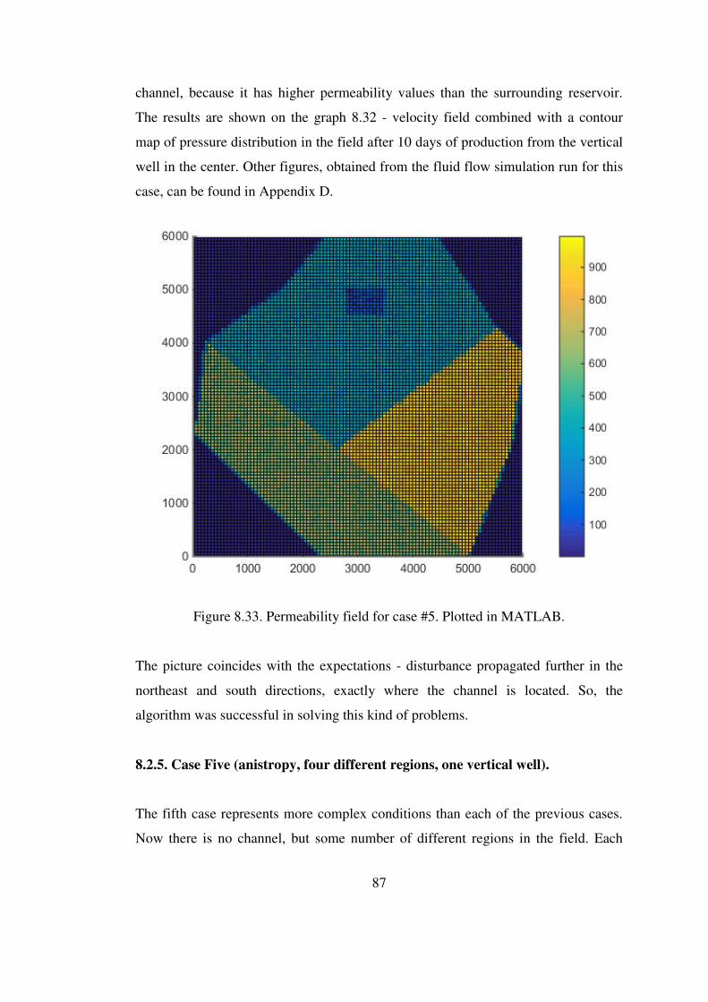
87
channel, because it has higher permeability values than the surrounding reservoir.
The results are shown on the graph 8.32 - velocity field combined with a contour
map of pressure distribution in the field after 10 days of production from the vertical
well in the center. Other figures, obtained from the fluid flow simulation run for this
case, can be found in Appendix D.
Figure 8.33. Permeability field for case #5. Plotted in MATLAB.
The picture coincides with the expectations - disturbance propagated further in the
northeast and south directions, exactly where the channel is located. So, the
algorithm was successful in solving this kind of problems.
8.2.5. Case Five (anistropy, four different regions, one vertical well).
The fifth case represents more complex conditions than each of the previous cases.
Now there is no channel, but some number of different regions in the field. Each
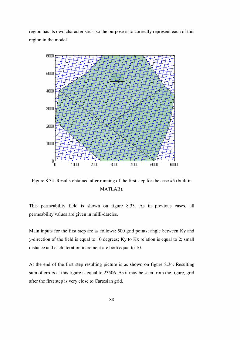
88
region has its own characteristics, so the purpose is to correctly represent each of this
region in the model.
Figure 8.34. Results obtained after running of the first step for the case #5 (built in
MATLAB).
This permeability field is shown on figure 8.33. As in previous cases, all
permeability values are given in milli-darcies.
Main inputs for the first step are as follows: 500 grid points; angle between Ky and
y-direction of the field is equal to 10 degrees; Ky to Kx relation is equal to 2; small
distance and each iteration increment are both equal to 10.
At the end of the first step resulting picture is as shown on figure 8.34. Resulting
sum of errors at this figure is equal to 23506. As it may be seen from the figure, grid
after the first step is very close to Cartesian grid.

89
Main inputs for the second step are: number of points that were changed during each
iteration is 5; 450 iterations; each point was allowed to move 8 times; as it was said,
four regions were introduced: one with permeabilities between 1 and 250 md, the
second with permeabilities between 251 and 500 md, the third with permeabilities
between 501 and 750 md, and the last one with permeabilities between 750 and 1000
md. These regions were shown on the figure 8.20.
Figure 8.35. Results obtained after running of the second step of case #5 (built in
MATLAB).
Resulting locations of grid points after the second step of the case #5 are shown at
figure 8.35. As in the previous cases, number of blocks is still the same as in figure
8.21, so change in the sum of errors is only because of the better placement of the
grid points. Sum of errors reduced here from the 23506 to 5872.

90
Figure 8.36. shows error values for all 450 generations of the fifth case. The curve
contiuouly goes down, reaches minimum in the early one hudred fourties and then
shows mainly upward trend.
Main inputs for the third step are: one vertical well in the center of the reservoir;
radius around the well that was repopulated is equal to 100 feet; 60 points related to
this well was added; distance between the first and the second layers of points
around the well is equal to 10 feet; distance to the next layers are 1.2 times the
distance to the previous one.
Figure 8.36. Error values for all generations of Case #5.
The obtained results are shown on figure 8.37. The resulting number of blocks is
equal to 530, while the sum of errors in all of the blocks reduced from an initial
value of 23506 to 5872, which is not so good as previous two cases, but still quite
impressive.
For this case fluid flow simulation run was also implemented. Inputs for the run are
exactly as in the previous cases: vertical well producing at 100 stb/d; initial reservoir
pressure equal to 3044 PSI; run for 5 days; time step 0.5 day.
0
5000
10000
15000
20000
25000
0 100 200 300 400 500
Su
m o
f E
rro
rs
Number of Generations
Case #5

91
Figure 8.37. Results obtained for the case #5 (built in MATLAB).
Figure 8.38. Velocity field combined with the contour map of the distribution of the
pressures after 2.5 days of production for the fifth case (obtained with Surfer).

92
Expectations are to see pressure disturbance propagating at a higher rate towards the
lower regions, because they have higher permeability values than the other regions.
The picture shown on figure 8.38 completely coincides with the expectations -
disturbance propagated further in the east and south directions, exactly where the
higher permeability regions are located. So, the algorithm was also successful in
solving this kind of problems. Other flow simulation run's timesteps can be found in
Appendix E.
Figure 8.39. Results obtained after running of the first step for the case #6 (built in
MATLAB).
8.2.6. Case Six (anisotropy, no heterogeneities, fault and horizontal well)
Case six, last case discussed in this thesis, represents conditions with
compartmentalized reservoir, from where production is performed using one
horizontal well.

93
The main purpose of showing of this case is to see, how the fault and horizontal well
are added to the model. Permeability field required for running of the algorithm is
the same as in cases #1 and #2.
Figure 8.40. Results obtained after running of the second step of case #6 (built in
MATLAB).
Main inputs for the first step are as follows: 600 grid points; angle between Ky and
y-direction of the field is equal to 90 degrees; Ky to Kx relation is equal to 2; small
distance is equal to 5, while each iteration distance increment is equal to 2.5.
Reservoir boundaries are chosen as in all of the previous cases.
At the end of the first step resulting picture is as shown on figure 8.39. Resulting
sum of errors at this figure is equal to 18317. As it may be seen from the figure, grid
after the first step is very close to Cartesian grid.

94
Main inputs for the second step are: number of points that were changed during each
iteration is 5; 320 iterations; each point was allowed to move 9 times; only one
permeability region with permeabilities between 1 and 1000 md is present.
Resulting locations of grid points after the second step of the case #5 are shown at
figure 8.40. As in the previous cases, number of blocks is still the same as in figure
8.39, so change in the sum of errors is only because of the better placement of the
grid points. Sum of errors reduced here from the 18317 to 2811.
Figure 8.41. Error values for all generations of Case #6.
Figure 8.41. shows error values for all 320 generations of the fourth case. The curve
contiuouly goes down, reaches minimum in the mid-sixties and then shows mainly
upward trend.
Main inputs for the third step are: one horizontal well and one sealing fault totally
dividing reservoir into two compartments (figure 8.42); radius around the well that
was repopulated is equal to 50 feet; 100 points related to this well were added;
distance between the first and the second layers of points around the well is equal to
5 feet; distance to the next layers are 1.2 times the distance to the previous one.
0
2000
4000
6000
8000
10000
12000
14000
16000
18000
20000
0 50 100 150 200 250 300 350
Su
m o
f E
rro
rs
Number of Generations
Case #6

95
The obtained results are shown on figure 8.42. The resulting number of blocks is
equal to 747, while the sum of errors in all of the blocks reduced from an initial
value of 18317 to 2811, which is also pretty impressive. Resulting number of blocks
is higher than the 600 entered in the first step because of the grid points related to
well and fault and also points related to proper reservoir border handling.
Figure 8.42. Results obtained for the case number six (built in MATLAB).
For this case fluid flow simulation run was not implemented, because the model that
was used for running of previous cases is still under construction and is not able to
handle horizontal wells at the moment of writing of this thesis work.
8.3. Effects of inputs on final results
This subchapter discusses effects of input values on final results by showing several
cases and talking about them. At the end of it, conclusion about how parameters
should be chosen in order to get less error values is made. Parameters chosen for this
study are all the parameters that affect final distribution of grid points, that can be

96
changed. Also no sensitivity study on to what extent each of the parameters affects
final result is made, so it is proposed to do it in the future studies.
8.3.1. Effect of number of grid points
It is obvious that higher amount of points should end up with less resulting error.
This is shown on figure 8.43.
The only difference in the cases shown in the figure is number of grid points, other
than that all input values were chosen to be absolutely the same. Background
petrophysical property mesh consists of 57600 uniformly distributed permeability
points with values randomly generated in the interval between 1 and 1000 md. As it
may be seen from the figure, while number of blocks is four times higher on the right
figure, error in there is approximately less by one-fifth. This difference is not very
big, however, from the figure it may be seen that reservoir boundary handling is
much better than in the left one, especially in the right lower corner.
Figure 8.43. Comparing results with different number of blocks (obtained with
MATLAB).
But this better accuracy comes at big price - calculation time of the second step,
which is the most time consuming step in the algorithm, differs significantly for

97
these two cases: left one requires 200 seconds in order to perform 100 generations,
while the right one requires 670 seconds for the same amount of generations. Also,
because right case has higher amount of grid points, more of them will require
relocation compared to the left case. This means that for the same input values, right
hand side will also require higher amount of generations in order to get to the
minimum error value that could be used as the final result. So, whether to use higher
amount of grid points is not an easy question.
8.3.2. Effect of number of moving grid points
As it was discussed in methodology, during each generation number of grid points
with highest error values are moved. This number is taken from the input given by
the person using the algorithm, so there is a question whether to give big values in
order to move several grid points at once, or limit them, for example, moving them
one by one. Figure 8.44 shows two cases that differ from each other only by this
criterion.
Figure 8.44. Comparing results with different number of movements for each grid
point (obtained with MATLAB).
In the case shown on the left grid points were moved one by one, while in the case
shown on the right ten worst grid points were chosen in each generation to be

98
moved. First case shows smaller final error value and that is what can be expected:
when high amount of point is moved during each generation, several points that are
not the worst are moved also with the worst one. The problem is that maybe better
result in terms of error function may have been achieved in the middle of moving.
That is why it is proposed to move less amount of grid points during each
generation. However, this choice also have drawbacks. The less amount of grid
points is moved during each generation, the more amount of generations may be
required to get best results, which affects significantly calculation time. Also it must
be said that moving several points in each generation also affects calculation time,
by affecting each generation calculation time. Left hand side case requires 105
seconds in order to calculate 100 generations, while right hand side case requires 140
seconds. This difference is not very big, but also should be considered.
Figure 8.45. Comparing results with different limits of movements (obtained with
MATLAB).
8.3.3. Effect of limit of movement of grid points
Another input criterion that affects final results is number of times each point can be
moved. This is a very important values, because it lets control at what distance may
point end up from its original place. The effect of this criteria is shown on figure
8.45.

99
As in the previous cases, these ones are also differ only in the input criterion that is
discussed - all other values are absolutely the same. As it can be seen from the figure
8.45, left hand side case, using limit of movement equal to ten, has smaller error
value at the end and also less distortion of the initial grid on the left and right sides
of the reservoir. As it was already said, limiting movement makes it possible to
control movement of points to some extent, which means that smaller value for this
criterion should end up in less grid distortion. However, by limiting number of
movements better results also may be missed. This criteria does not affect
computation time, so it must be carefully considered whether to let points to move
freely in the reservoir or to limit them.
Figure 8.46. Comparing results with different distance of movement (obtained with
MATLAB).
8.3.4. Effect of distance of movement of grid points
Finally, the last criterion that affects final result - distance at which points are
moved. As it was mentioned in the methodology chapter, input also includes fraction
of longer distance that points are moved at. Longer distance is the distance between
neighboring grid points in the direction of lower permeability. The effect of this
criterion is shown in the figure 8.46.
100
It seems like the distance at which points are moved during each iteration should be
chosen as little in order to get better results. However, cases show something
opposite to this supposition. Error of the case with distance of movement equal to
0.01 times the big distance has higher final error values than the case with 0.07 times
the big distance. It also can be seen from the figure, right hand side case deals with
reservoir properties in a more accurate way than the left hand side case. This can be
seen especially in the lower left corner. The only advantage of smaller moving
distance seems to be less distortion of the initial grid. So, proposition would be to
use something in between of these values, but the choice totally depends on the
person using the algorithm.
In the next chapter conclusion and propositions for future studies can be found.

101
CHAPTER 9
CONCLUSION
Based on the results obtained after running of cases of increasing complexity,
algorithm described in this thesis proved to be capable of placing Voronoi grid
points in reservoir simulation in order to honor geological properties of the reservoir
including anisotropy orientation and ratio, and reservoir heterogeneities.
One of the main advantages of the algorithm is that it tries to obtain better locations
of limited number of Voronoi grid points without making a significant increase in
this number. This means that instead of increasing the number of grid points
exceedingly, it provides better solutions rather than placing these points uniformly
all over the field. Error values and graphs that show final distribution of the grid
plots show that as the grid block boundaries coincide with background reservoir
property mesh, error values decrease.
Also it must be mentioned that effectiveness of the algorithm in terms of error
function can be affected by values of some input parameters required for running of
the algorithm. The most effective inputs include the number of times that the points
are allowed to move as less points to be moved during each iteration, but a greater
number of times and therefore with more iterations. Number of grid points also
affects final accuracy - the higher the number of grid points the better is the result.
However, these choices will increase computation time, so they must be carefully
chosen before application of the algorithm to the problem.

102

103
CHAPTER 10
PROPOSITION FOR FUTURE STUDIES
For future studies it is proposed to use the algorithm on the cases of increasing
complexity and to add all necessary sophistications to the algorithm so that all the
complications will be solved.
This includes:
Trying to change algorithm, so that not only one property would be used for
differentiating different geological entities. In this study only permeability
was used for this purpose, proposition is to use several different properties
together at one time. Maybe some weightening of these properties should be
applied to each of the property points.
Considering application of the algorithm to 3D problems, including not
horizontal formations.
Considering handling of regions with intersecting intervals of property
values.
Thinking if a better error function definition could be used.
Checking of the results obtained for the case with horizontal wells by running
flow simulation.
Do similar flow simulation runs with Cartesian grid and compare the results
for all of the cases.
Thinking if the grid points near the reservoir boundaries can be handled
better. Maybe truncation concept can be used there, which will further
decrease number of grid points.

104
Doing sensitivity analysis on to what extent each of the input parameters
affects final result.

105
BIBLIOGRAPHY
Adamson, G. et al. (1996), "Simulation Throughout the Life of the Reservoir",
Oilfield Review, Summer 1996, pp. 16-27.
Alpay, Allen, O. (1972), "A Practical Approach to Defining Reservoir Heterogeneity", Journal of Petroleum Technology, July, 1992, pp. 841-848. Anderson, B. et al. (1994), "Oilfield Anisotropy: Its Origins and Electrical Characteristics", Oilfield Review, October 1994, pp. 48-56. Angelo, G. D., Henning, T. and Kley, W. (2002), "Nested-grid Calculations of Disk-Planet Interaction", January 2002. Antoniou, A. and Lu, W. (2007), "Practical Optimization. Algorithms and Engineering Applications", Springer Science+Business Media, LLC, 2007. Aurenhammer, F. (1991), "Voronoi Diagrams - a survey of a fundamental geometric data structure", ACM Comput. Surv., 1991. Aurenhammer, F. and Klein, R. (2000), "Voronoi Diagrams. Handbook of Computational Geometry", Ed. J. Sack, J. Urrutia (eds.), 2000, 201-290. Aziz, K. and Settari, A. (1979), "Petroleum Reservoir Simulation", Appled Science Publishers, London. Aziz, K. (1993), "Reservoir Simulation Grids: Opportunities and Problems", Journal of Petroleum Technology, July 1993, pp. 658-663. Baldick, R. (2006), "Applied Optimization. Formulation and Algorithms for Engineering Systems", Cambridge University Press, 2006. Belegundu, A. D. and Chandrupatla T. R. (2011), "Optimization Concepts and Applications in Engineering", 2nd Ed., Cambridge University Press, 2011. Beni, L. H., Mostafavi, M.A. and Pouliot, J. (2010). "Voronoi diagram: An adaptive spatial tessellation for processes simulation, Modeling Simulation and Optimization - Tolerance and Optimal Control, Shkelzen Cakaj (Ed.), ISBN: 978-953-307-056-8, InTech, Available from: http://www.intechopen.com/books/modeling-simulation-and-optimization-tolerance-and-optimalcontrol/voronoi-diagram-an-adaptive-spatial-tessellation-for-processes-simulation, retrieved on 25th of August, 2015.

106
Bernal, J. (1993), "Bibliographic Notes on Voronoi Diagrams", Technical report, National Institute of Standarts and Technologies, April 1993. Branets, L. V., Ghai, S. S., Lyons, S. L. and Wu, X.-H. (2009), "Efficient and Accurate Reservoir Modelling Using Adaptive Gridding With Global Scale Up", SPE paper 118946, Society of Petroleum Engineers, 2009. Castellini, A. (2001), "Flow Based Grids For Reservoir Simulation", MSc Dissertation, Stanford University, Stanford, June 2001. Castillo, J. E. (1991), "Mathematical Aspects of Grid Generation", Society for Industrial and Applied Mathematics, Philadelphia, 1991. Chawner, J. (2013), "Quality and Control - Two Reasons Why Structured Grids Are Not Going Away", The Connector Pointwise, March / April, 2013. Chong, E. K. P. and Zak, S. H. (2008), "An Introduction to Optimization", 3rd Ed., John Wiley & Sons, Inc., 2008. Corvi, P. et al. (1992), "Reservoir Characterization Using Expert Knowledge, Data and Statistics", Oilfield Review, January 1992, pp. 25-39. Diwekar, U. (2008), "Introduction to Applied Optimization", 2nd Ed., Springer Science+Business Media, LLC, 2008. Du, Q., Faber, V. and Gunzburger, M. (1999), "Centroidal Voronoi Tesellations: Applications and Algorithms", SIAM Review, Vol. 41, No. 4, pp. 637-676, Society for Industrial and Applied Mathematics. Ertekin, T., Abou-Cassem, J. H. and King G. R. (2001), "Basic Applied Reservoir Simulation", Henry L. Doherty Memorial Fund of AIME Society of Petroleum Engineers, Richardson, Texas, 2001. Evazi, M. and Mahani, H. (2009), "Generation of Voronoi Grid Based on Vorticity for Coarse-Scale Modeling of Flow in Heterogeneous Formations", Springer Science+Business Media B.V. 2009. Forsyth, P. (1989), "A Control Volume Finite Element Method for Local Mesh Refinements", SPE 18415, 10th SPE Symposium Reservoir Simulation. Frederick, C.O., Wong, Y.C. and Edge, F.W. (1970), "Two-Dimensional Automatic Mesh Generation for Structural Analysis", Int. J. Nurner, Meth. Eng. 1970, 2, No 1, pp. 133-144. Fung, L. S. K., Ding, X. Y. and Dogru, A. H. (2014), "Unconstrained Voronoi Grids for Densely Spaced Complex Wells in Full-Field Reservoir Simulation", SPE paper 163648, SPE Journal 2014.

107
Galloway, W. A., and D. K. Hobday (1996), "Terrigenous Clastic Depositional System", 2ed. Springer-Verlag, New York, 1996. George, P. L. (1991), "Automatic Mesh Generation", 1991. Heinemann, Z. E. and Brand, C.W. (1989), "Gridding Techniques in Reservoir Simulation", presented at the 1989 Second Interntional Forum on Reservoir Simulation, Alpbach. Heinemann, Z. E., Brand, C.W., Munka, M. and Chen, Y. (1991), "Modeling reservoir geometry with irregular grids", SPE Reservoir Engineering, 6(2), May 1991. Hirasaki, G. J. and O'Dell P. M. (1970), "Representation of Reservoir Geometry for Numerical Simulation", SPEJ, December 1970, p. 393. Ho-Le, K. (1988), "Finite Element Mesh Generation Methods a Review and Classification", Computer-Aided Design (Jan.-Feb 1988) 20, pp. 27-38. Islam, M.R., et al. (2010), "Advanced Petroleum Reservoir Simulation", Scrivener Publishing LLC, 2010. Jensen, J.L., et al. (1997), "Statistics for Petroleum Engineers and Geoscientists", Prentice-Hall, Inc., 1997. Kang, J. M. (2008), "Voronoi Diagrams", 8715: Spatial Databases Encyclopedia Article. Katzmayr, M. and Ganzer, L. (2009), "An Iterative Algorithm for Generating Constrained Voronoi Grids", SPE paper 118942, Society of Petroleum Engineers. Kaufmann, D. E. (2006), "Capability Development for Modeling the Structure and Dynamics of Barred Spiral Galaxies 15-R9577", Southwest Research Institute, 2006. Kilic, A. and Ertekin, T. (2003), "Application of a Local Grid Refinement Protocol in Highly Faulted Reservoir Architectures", Journal of Canadian Petroleum Technology, April 2003, Volume 42, No. 4, pp. 58-69. Kocberber, S., (1997), "An Automatic, Unstructured Control Volume Generation System for Geologically Complex Reservoirs", SPE paper 38001, Society of Petroleum Engineers, 1997. Kuwauchi, Y. et al. (1996), "Development and Applications of a Three Dimensional Voronoi-Based Flexible Grid Black Oil Reservoir Simulator", SPE paper 37028, Society of Petroleum Engineers, 1996.
108
Lake, L.W. and Holstein, E. D. (2007), "Petroleum Engineering Handbook", Vol. 5 - Reservoir Engineering and Petrophysics, Society of Petroleum Engineers. Li, Q., Li, H., Cai, Q. and Liu, Y. (2011), "Generation of 2D Conforming Voronoi Diagram in Complex Domain", J. Chang (Ed.): ICAIC 2011, Part IV, CCIS 227, pp. 32-39, Springer-Verlag Berlin Heidelberg, 2011. Mackay, A. L. (1972), "Stereological Characteristics of Atomic Arrangements in Crystals", Journal of Microscopy, 1972, 95, 217-227. Manrique J. F., Kasap E. and Georgi D.T. (1994), "Effect of Heterogeneity and Anisotropy on Probe Permeameter Measurements", Transactions of the SPWLA 35th Annual Logging Symposium, Tulsa, Oklahoma, USA, June 19-22, 1994. Marcondes, F., Maliska, C. R. and Zambaldi, M. C. (2009), "A comparative study of implicit and explicit methods using unstructured voronoi meshes in petroleum reservoir simulation", Journal of The Brazilian Society of Mechanical Sciences and Engineering, October/December 2009. Mattax, C. C. and Dalton R. L. (1990), "Reservoir Simulation", SPE monograph, Vol. 13, Henry L. Doherty Series, 1990. Mavriplis, D. J. (1996), "Mesh Generation and Adaptivity for Complex Geometries an Flows", Handbook of Computational Fluid Mechanics, 1996. McNeal, R. H. (1953), "An Asymmetrical Finite Difference Network", Quart. Appl. Math, 1953, 11, 295-310. Merland, R. et al. (2011), "Building Centroidal Voronoi Tessellations For Flow Simulation In Reservoirs Using Flow Information", SPE paper 141018, Society of Petroleum Engineers, 2011. Merland, R., Caumon, G., Levy, B. and Collon-Drouaillet, P. (2014), "Voronoi Grids Conforming to 3D Structural Features", Springer International Publishing Switzerland, 2014. Mlachnik, M. J., Durlofsky, L. J. and Heinemann, Z. E. (2006), "Sequentially Adapted Flow-Based PEBI Grids for Reservoir Simulation", SPE paper 90009, Society of Petroleum Engineers, 2006. Moog, G. J. E. A. (2013), "Advanced Discretization Methods for Flow Simulation Using Unstructured Grids", PhD dissertation, Stanford University, Stanford, June 2013. Odeh, A. S. (1982), "An overview of mathematical modeling of the behavior of hydrocarbon reservoirs", SIAM Review, Vol. 24 (3), pp. 263.

109
Okabe, A. et al. (2000), "Spatial Tesselations: Concepts and Applications of Voronoi diagrams", 2nd Ed., Probability and Statistics, Wiley, 2000. Olorode, O. M. (2011), "Numerical Modeling of Fractured Shale-Gas and Tight-Gas Reservoirs Using Unstructured Grids", MSc Thesis, Texas A&M University, Austin, December 2011. Palagi, C. L. (1992), "Generation and Application of Voronoi Grid to Model Flow in Heterogeneous Reservoirs", PhD Dissertation, Stanford University, Stanford, May 1992. Palagi, C. L. and Aziz, K. (1993), "The Modeling of Vertical and Horizontal Wells With Voronoi Grid", SPE paper 24072, Society of Petroleum Engineers, 1993. Palagi, C. L. and Aziz, K. Appendix (1993), "The Modeling of Vertical and Horizontal Wells With Voronoi Grid", SPE paper 26301, Society of Petroleum Engineers, 1993. Palagi, C. L., P.R. Ballin and Aziz K. (1993), "The Modeling of Flow in Heterogeneous Reservoirs With Voronoi Grid", SPE paper 25259, Society of Petroleum Engineers, 1993. Palagi, C. L. and Aziz, K. (1994), "Use of Voronoi Grid in Reservoir Simulation", SPE paper 22889, SPE Advanced Technology Series, Vol. 2, No. 2. Palagi, C. L. and Aziz, K. Appendix (1994), "Use of Voronoi Grid in Reservoir Simulation: Appendices A, B and C", SPE paper 26951, Society of Petroleum Engineers, 1994. Pathak, P. et al. (1980), "Rock Structure and Transport There in: Unifying with Voronoi Models and Percolation Concepts", SPE paper 8846, Society of Petroleum Engineers, April, 1980. Pedrosa, O.A. and Aziz, K. (1985), "Use of hybrid grid in reservoir simulation", proceedings of SPE Middle East Oil Technical Conference, pp. 99-12, Bahrain Pedrosa, O. A. and Aziz, K. (1986), "Use of a Hybrid Grid in Reservoir Engineering", SPE Reservoir Engineering, November 1986, pp. 611-621. Pedrosa, O. A. (1984), "Use of Hybrid Grid in Reservoir Simlation", PhD Dissertation, Stanford University, Stanford, December 1984. Ponting, D. K. (1989), "Corner Point Geometry in Reservoir Simulation", 1st European Conference on the Mathematics of Oil Recovery, July 1989. Prevost, M. (2003), "Accurate Coarse Reservoir Modeling Using Unstructured Grids, Flow-Based Upscaling and Streamline Simulation", PhD Dissertation, Stanford University, Stanford, December 2003.

110
Prevost, M., Lepage, F., Durlofsky, L. J. and Mallet, J.-L. (2004), "Unstructured 3D Gridding and Upscaling for Coarse Modelling of Geometrically Complex Reservoirs", 9th European Conference on the Mathematics of Oil Recovery, Cannes, France, 2004. Prothero, D. R. and Schwab, F. (2014), "Sedimentary Geology. An introduction to Sedimentary Rocks and Stratigraphy", 3rd Ed., W. H. Freeman and Company, 2014. Pruess, K. and Bodvarsson, G. S. (1983), "A Seven Point Finite Difference Method for Improved Grid Orientation Performance in Pattern Steamfloods", SPE paper 12252, 1983. Pyrcz, M. J. and Deutsch, C. V. (2014), "Geostatistical Reservoir Modeling", 2nd Ed., Oxford University Press, 2014. Rajan V. S. V (1988), "Discussion of the origins of Anisotropy", SPE paper 18394m, Journal of Petroelum Technology, July 1988, p. 905. Richards, F. D. (1974), "The Interpretation of Protein Structures: Total Volume, Group Volume Distributions and Packing Density", Journal of Molecular Biology, 1974, 82. Robertson, G. E. and Woo, P. T. (1978), "Grid-Orientation Effects and the Use of Orthogonal Curvilinear Coordinates in Reservoir Simulation", SPEJ, February 1978, p. 13. Sarvottamananda, S. (2010), "Voronoi Diagrams", Ramakrishna Mission Vivekananda University, BHU-IGGA, 2010. Slatt, R. M. (2006), "Stratigraphic Reservoir Characterization", Elsevier B. V., 2006. Soleng, H. H. and Holden, L., "Gridding for Petroleum Reservoir Simulation", Norwegian Computing Center. Sonier, F. and Chaumet, P. (1974), "A Fully Three-Dimensional Model In Curvilinear Coordinates", SPEJ, August 1974, p. 361. Syihab, Z. (2009), "Simulation of Discrete Fracture Network Using Flexible Voronoi Gridding", PhD Dissertation, Texas A&M University, Austin, December 2009. Todd, M. R., O'Dell, P. R. and Hirasaki, G. J. (1972) "Methods for Increased Accuracy in Numerical Reservoir Simulators", Trans. Society of Petroleum Engineers of AIME, 253, 515-530. Trease, H. E. (1985), "Three-Dimensional Free Langrangian Hydrodynamics", The Free-Language Method, eds. M. J. Fritts, W. P. Crowley and H. E. Trease, Lecture Notes in Physics, Springer-Verlag, New York, 1985, 238, 145-157.
111
Verma, S. K. (1996), "Flexible Grids for Reservoir Simulation", PhD Dissertation, Stanford University, Stanford, June 1996. Vestergaard, H., Olsen, H., Sikandar, A. S., Al-Emadi, I. A. and Noman, R. (2008) "Unstrucuctured Gridding for Full-Field Simulation of a Giant Carbonate Reservoir DEveloped With Long Horizontal Wells", Journal of Petroleum Technology, July, 2008. Voronoi, G. (1908), "Nouvelles applications des parametres continus a la theorie des formes quadratiques", J. Reine Angew. Math., 1908, 134, 198-287. Wadsley, A. W., Erlandsen, S. and Goemans, H. W. (1990), "HEX - A Tool for Integrated Fluvial Architecture Modelling and Numerical Simulation of Recovery Processes", The Norwegian Institute of Technology, North Sea Oil Reservoirs - II, 1990. Weber, K.J. (1986), "How heterogeneity affects oil recovery", in L. W. Lake and H. B. J. Carroll, eds., Reservoir Characterization: Orlando, FL, Academy Press, p. 487-844. Weise, T. (2011), "Global Optimization Algorithms - Theory and Application", 3rd Ed., Thomas Weise, 2011. Winterfield, P. H. et al. (1981), "Percolation and Conductivity of Random Two-Dimensional Composites", J.Phys. C.: Solid State Phys., 1981, 14, 2361-76. Yang, X. (2008), "Introduction to Mathematical Optimization. From Linear Programming to Metaheuristics", Cambridge International Science Publishing, 2008. Yang, X. and Koziel, S. (2011), "Computational Optimization and Applications in Engineering and Industry", Springer-Verlag Berlin Heidelberg, 2011.

112

113
APPENDIX A
SOURCE CODE
%{
This code was written as a part of a METU MSc dissertation of Ulvi
Rza-Guliyev.
To run it, four column vectors named permXvec, permYvec, permZvec,
permeabilitiesVec must already be loaded onto workspace of Matlab. permXvec,
permYvec and permZvec must have X, Y and Z coordinates of permeability
points in the field, while permeabilitiesVec must have permeability values
in x direction in it. All other inputs are given in the code.
%}
% Start of the first step, where initial population of the gridpoints is
% generated
n=input('Enter number of points: ');
angle=input('Enter value of Tetta, 0-360, degrees: ');
tet=pi*angle/180; % Changed to radians for trigonometric functions
if (tet < pi/2)
w=0;
elseif (tet >= pi/2 && tet < pi)
w=pi/2;
elseif (tet >= pi && tet < 3*pi/2)
114
w=pi;
elseif (tet >= 3*pi/2 && tet < 2*pi)
w=3*pi/2;
elseif tet == 2*pi
tet=0;
w=0;
else fprintf('Angle must be between 0 and 360 degrees. Start again.');
end
m=input('Enter Ky/Kx value: ');
kykxrel=m;
R=input('Enter distance in minimum direction (should be small): ');
increment=input('Enter value of increment to the minimum distance,\nthat will be
added at the end of each iteration: ');
% Entering reservoir vertexes
resBouVert=zeros;
nprb=input('Enter number of reservoir verteces: ');
for kl=1:1:nprb
resBouVert(kl,1)=input('Enter x coordinate of vertex: ');
resBouVert(kl,2)=input('Enter y coordinate of vertex: ');
end
resBouVert(nprb+1,1)=input('Enter x coordinate of first vertex: ');
resBouVert(nprb+1,2)=input('Enter y coordinate of first vertex: ');
resVertX=resBouVert(:,1);
resVertY=resBouVert(:,2);
% Calculating of rectangle boundaries
length=abs(max(resVertX)-min(resVertX));
width=abs(max(resVertY)-min(resVertY));
resVertX=resVertX-min(resVertX);
resVertY=resVertY-min(resVertY);

115
counter=n+1;
while counter>n
if m > 1 && tet >= 0 && tet < pi/2
Ry=R;
Rx=m*R;
elseif m > 1 && tet >= pi/2 && tet < pi
Ry=m*R;
Rx=R;
elseif m > 1 && tet >= pi && tet < 3*pi/2
Ry=R;
Rx=m*R;
elseif m > 1 && tet >= 3*pi/2 && tet < 2*pi
Ry=m*R;
Rx=R;
elseif m < 1 && tet >= 0 && tet < pi/2
Rx=m*R;
Ry=R;
elseif m < 1 && tet >= pi/2 && tet < pi
Ry=m*R;
Rx=R;
elseif m < 1 && tet >= pi && tet < 3*pi/2
Rx=m*R;
Ry=R;
elseif m < 1 && tet >= 3*pi/2 && tet < 2*pi
Ry=R;
Rx=m*R;
else
Rx=R;
Ry=R;
end

116
% Now it will calculate dimensions of matrix.
if (tet > 0 && tet < pi/2)
overwidth=width*cos(tet)+length*sin(tet);
overlength=width*sin(tet)+length*cos(tet);
matrixNreal=overlength/Rx;
matrixMreal=overwidth/Ry;
elseif (tet > pi && tet < 3*pi/2)
overwidth=width*cos(tet-pi)+length*sin(tet-pi);
overlength=width*sin(tet-pi)+length*cos(tet-pi);
matrixNreal=overlength/Rx;
matrixMreal=overwidth/Ry;
elseif (tet > pi/2 && tet < pi)
overlength=width*cos(tet-pi/2)+length*sin(tet-pi/2);
overwidth=width*sin(tet-pi/2)+length*cos(tet-pi/2);
matrixNreal=overwidth/Rx;
matrixMreal=overlength/Ry;
elseif (tet > 3*pi/2 && tet < 2*pi)
overlength=width*cos(tet-3*pi/2)+length*sin(tet-3*pi/2);
overwidth=width*sin(tet-3*pi/2)+length*cos(tet-3*pi/2);
matrixNreal=overwidth/Rx;
matrixMreal=overlength/Ry;
elseif (tet == 0 || tet == pi || tet == 2*pi)
matrixNreal=width/Ry;
matrixMreal=length/Rx;
elseif (tet == pi/2 || tet == 3*pi/2)
matrixNreal=width/Rx;
matrixMreal=length/Ry;
else fprintf('Angle must be between 0 and 360 degrees. Start again.');
end
matrixN=ceil(matrixNreal);
matrixM=ceil(matrixMreal);

117
abscissa=zeros(matrixN,matrixM);
ordinate=zeros(matrixN,matrixM);
% Now it will calculate starting point, which is outside of reservoir.
if (tet > 0 && tet < pi/2)
Sx=0-width*sin(tet)*cos(tet);
Sy=width*sin(tet)*sin(tet);
elseif (tet > pi/2 && tet < pi)
Sx=0-width*sin(tet-pi/2)*cos(tet-pi/2);
Sy=width*sin(tet-pi/2)*sin(tet-pi/2);
elseif (tet > pi && tet < 3*pi/2)
Sx=0-width*sin(tet-pi)*cos(tet-pi);
Sy=width*sin(tet-pi)*sin(tet-pi);
elseif (tet > 3*pi/2 && tet < 2*pi)
Sx=0-width*sin(tet-w)*cos(tet-w);
Sy=width*sin(tet-w)*sin(tet-w);
elseif (tet == 0 || tet == pi/2 || tet == pi || tet == 3*pi/2 || tet == 2*pi)
Sx=0;
Sy=0;
else fprintf('Angle must be between 0 and 360 degrees. Start again.');
end
% Start of generation of probable initial population of gridpoints
if (tet > 0 && tet < pi/2 ) || (tet > pi && tet < 3*pi/2)
for i=1:1:matrixN
abscissa(i,1)=Sx;
ordinate(i,1)=Sy;
for e=2:1:matrixM
abscissa(i,e)=abscissa(i,e-1)+Ry*sin(tet-w);
ordinate(i,e)=ordinate(i,e-1)+Ry*cos(tet-w);
end
Sx=Sx+Rx*cos(tet-w);
118
Sy=Sy-Rx*sin(tet-w);
end
elseif (tet > pi/2 && tet < pi) || (tet > 3*pi/2 && tet < 2*pi);
for i=1:1:matrixN
abscissa(i,1)=Sx;
ordinate(i,1)=Sy;
for e=2:1:matrixM
abscissa(i,e)=abscissa(i,e-1)+Ry*sin(tet-w);
ordinate(i,e)=ordinate(i,e-1)+Ry*cos(tet-w);
end
Sx=Sx+Rx*cos(tet-w);
Sy=Sy-Rx*sin(tet-w);
end
elseif (tet == 0 || tet == pi)
for i=1:1:matrixN
abscissa(i,1)=Sx;
ordinate(i,1)=Sy;
for e=2:1:matrixM
ordinate(i,e)=ordinate(i,e-1)+Rx*sin(tet-w);
abscissa(i,e)=abscissa(i,e-1)+Rx*cos(tet-w);
end
Sy=Sy+Ry*cos(tet-w);
Sx=Sx+Ry*sin(tet-w);
end
elseif (tet == pi/2 || tet == 3*pi/2)
for i=1:1:matrixN
abscissa(i,1)=Sx;
ordinate(i,1)=Sy;
for e=2:1:matrixM
ordinate(i,e)=ordinate(i,e-1)+Ry*sin(tet-w);
abscissa(i,e)=abscissa(i,e-1)+Ry*cos(tet-w);
end

119
Sy=Sy+Rx*cos(tet-w);
Sx=Sx+Rx*sin(tet-w);
end
else fprintf('Angle must be between 0 and 360 degrees');
end
v=1;
sk=matrixN*matrixM;
absc=zeros(sk,1);
ord=zeros(sk,1);
% Deleting of the points outside of rectangle
for i=1:1:matrixN
for e=1:1:matrixM
if abscissa(i,e)>0 && abscissa(i,e)<=length ...
&& ordinate(i,e)>0 && ordinate(i,e)<=width
absc(v,1)=abscissa(i,e);
ord(v,1)=ordinate(i,e);
v=v+1;
end
end
end
% Means of seeing how many points were generated in current iteration
fprintf('Number of blocks on this stage is: %g\n', v);
if m>=1
fprintf('At this stage your minimum distance is: %g\n', R);
else
fprintf('At this stage your minimum distance is: %g\n', m*R);
end
tocontinue=input('Press 0 + enter:');

120
counter=v;
if v>n
R=R+increment;
else fprintf('Number of blocks is: %g\n', counter-1);
end
end
% Saving of the final initial population in allGens
numGen=1;
allGens{numGen,1}=absc;
allGens{numGen,2}=ord;
% Inputs for the second step
lastNumPoints=input('Enter number of points that will be changed in every iteration:
');
moveFun=input('Enter fraction of distance that points will be moved (i.e. 0.07): ');
requiredNumGen=input('Enter required number of generations: ');
requiredError=input('Enter required error: ');
limitOfMovement=input('Enter required number of movements for each point: ');
numReg=input('Enter number of regions (without zero region): ');
minLim=zeros;
maxLim=zeros;
for kg=1:1:numReg
fprintf('Enter minimum permeability in region #%g: ',kg);
minLim(kg,1)=input('');
fprintf('Enter maximum permeability in region #%g: ',kg);
maxLim(kg,1)=input('');
end
minLim(kg+1,1)=0;
maxLim(kg+1,1)=abs(min(minLim)-1);
numberOfMovements=zeros(counter-1,1);

121
sumError=requiredError+1;
checker21=1;
permXi=size(permXvec,1);
permFieldVec=[permXvec,permYvec];
if m*R>=R
maxDist=m*R;
minDist=R;
else
maxDist=R;
minDist=m*R;
end
stopStep2=0;
minimEr=inf;
while sumError>=requiredError && numGen<=requiredNumGen+1 &&
stopStep2~=42
num=1;
number=1;
x=zeros(counter-1,1);
y=zeros(counter-1,1);
z=40*ones(counter-1,1);
absc=[absc;0];
ord=[ord;0];
while absc(num,1)~=0
absc(num,1)=roundn(absc(num,1),-3);
x(num,1)=absc(num,1);
num=num+1;
end
while ord(number,1)~=0
ord(number,1)=roundn(ord(number,1),-3);
y(number,1)=ord(number,1);

122
number=number+1;
end
xy=[x,y];
blocksOfPoints=zeros(permXi,counter-1);
distances=pdist2(permFieldVec,xy);
% Finding which block each permeability point is related to
for kk=1:1:size(distances,1)
distancesForPoints=distances(kk,:);
backUpDist=distancesForPoints;
[closestDist,ind]=min(backUpDist);
blocksOfPoints(kk,ind)=permeabilitiesVec(kk,1);
backUpDist(1,ind)=inf;
[closestDist2,ind2]=min(backUpDist);
if closestDist2==closestDist
blocksOfPoints(kk,ind2)=permeabilitiesVec(kk,1);
backUpDist(1,ind2)=inf;
[closestDist3,ind3]=min(backUpDist);
if closestDist3==closestDist2
blocksOfPoints(kk,ind3)=permeabilitiesVec(kk,1);
backUpDist(1,ind3)=inf;
[closestDist4,ind4]=min(backUpDist);
if closestDist4==closestDist3
blocksOfPoints(kk,ind4)=permeabilitiesVec(kk,1);
backUpDist(1,ind4)=inf;
[closestDist5,ind5]=min(backUpDist);
if closestDist5==closestDist4
blocksOfPoints(kk,ind5)=permeabilitiesVec(kk,1);
backUpDist(1,ind5)=inf;
[closestDist6,ind6]=min(backUpDist);
if closestDist6==closestDist5
123
blocksOfPoints(kk,ind6)=permeabilitiesVec(kk,1);
backUpDist(1,ind6)=inf;
[closestDist7,ind7]=min(backUpDist);
if closestDist7==closestDist6
blocksOfPoints(kk,ind7)=...
permeabilitiesVec(kk,1);
backUpDist(1,ind7)=inf;
[closestDist8,ind8]=min(backUpDist);
if closestDist8==closestDist7
blocksOfPoints(kk,ind8)=...
permeabilitiesVec(kk,1);
backUpDist(1,ind8)=inf;
[closestDist9,ind9]=min(backUpDist);
if closestDist9==closestDist8
blocksOfPoints(kk,ind9)=...
permeabilitiesVec(kk,1);
backUpDist(1,ind9)=inf;
[closestDist10,ind10]=min(backUpDist);
if closestDist10==closestDist9
fprintf('Something is wrong');
end
end
end
end
end
end
end
end
end
end
jj=1;

124
forError=0;
uu=1;
error=zeros(counter-1,1);
% Calculating of error for each block
while jj<=counter-1
for ii=1:1:permXi
if blocksOfPoints(ii,jj)~=0;
forError(uu,1)=blocksOfPoints(ii,jj);
uu=uu+1;
end
end
for ht=1:1:size(minLim,1)
if forError(1,1)>=minLim(ht,1) && forError(1,1)<=maxLim(ht,1)
blockMin=minLim(ht,1);
blockMax=maxLim(ht,1);
end
end
ug=0;
for hk=1:1:size(forError)
if forError(hk,1)>=blockMin && forError(hk,1)<=blockMax
ug=ug+1;
end
end
if ug==size(forError,1)
error(jj,1)=0;
elseif ug<size(forError,1)
error(jj,1)=std(forError);
else fprintf('Something is wrong(line 346)');
end
checker{jj,checker21}=forError;
jj=jj+1;

125
uu=1;
forError=0;
end
% Saving errors in allGens
allGens{numGen,3}=error;
sumError=sum(error);
allGens{numGen,4}=sumError;
if minimEr>sumError
minimEr=sumError;
elseif sumError>=minimEr+2000
stopStep2=42;
end
% Assigning of fitnesses
errorBackUp=error;
fitness=zeros(counter-1,1);
ii=1;
while ii<=counter-1
[value,index]=min(errorBackUp);
fitness(index,1)=ii;
errorBackUp(index,1)=inf;
ii=ii+1;
end
xBackUp=x;
yBackUp=y;
pp=counter-1;
dd=0;
% Moving of bad points in the required direction while checking if number
% of movements for these points is less than the limit

126
while dd<=lastNumPoints && pp>=2
for index=1:1:counter-1
if fitness(index,1)==pp
ppm=zeros(numReg+1,1);
if numberOfMovements(index,1)<limitOfMovement;
numberOfMovements(index,1)=numberOfMovements(index,1)+1;
dd=dd+1;
blm=checker{index,checker21};
% Calculates how many points inside block are of different
% regions permeability.
for zv=1:1:size(blm,1)
for fq=1:1:numReg
if blm(zv,1)==0.001
ppm(numReg+1)=ppm(numReg+1)+1;
elseif blm(zv,1)<=maxLim(fq,1) && blm(zv,1)>=minLim(fq,1)
ppm(fq,1)=ppm(fq,1)+1;
else moe=42;
end
end
end
xes=zeros;
yes=zeros;
skp=1;
[valper,indper]=max(ppm);
useMin=minLim(indper,1);
useMax=maxLim(indper,1);
for jkr=1:1:size(permeabilitiesVec,1)
if (blocksOfPoints(jkr,index)<useMin &&
blocksOfPoints(jkr,index)>0) || (blocksOfPoints(jkr,index)>useMax)
xes(skp,1)=permXvec(jkr,1);
yes(skp,1)=permYvec(jkr,1);
skp=skp+1;
127
end
end
centX=mean(xes);
centY=mean(yes);
myPointX=x(index,1);
myPointY=y(index,1);
bcatm1=abs(centX-myPointX);
bcatm2=abs(centY-myPointY);
xuse=myPointX-centX;
yuse=myPointY-centY;
if xuse>0 && yuse>0
alpha=atand(bcatm2/bcatm1);
x(index,1)=x(index,1)+maxDist*moveFun*cosd(alpha);
y(index,1)=y(index,1)+maxDist*moveFun*sind(alpha);
elseif xuse<0 && yuse>0
alpha=atand(bcatm2/bcatm1);
x(index,1)=x(index,1)-maxDist*moveFun*cosd(alpha);
y(index,1)=y(index,1)+maxDist*moveFun*sind(alpha);
elseif xuse>0 && yuse<0
alpha=atand(bcatm2/bcatm1);
x(index,1)=x(index,1)+maxDist*moveFun*cosd(alpha);
y(index,1)=y(index,1)-maxDist*moveFun*sind(alpha);
elseif xuse<0 && yuse<0
alpha=atand(bcatm2/bcatm1);
x(index,1)=x(index,1)-maxDist*moveFun*cosd(alpha);
y(index,1)=y(index,1)-maxDist*moveFun*sind(alpha);
elseif xuse==0 && yuse>0
x(index,1)=x(index,1);
y(index,1)=y(index,1)+maxDist*moveFun;
elseif xuse==0 && yuse<0
x(index,1)=x(index,1);
y(index,1)=y(index,1)-maxDist*moveFun;
128
elseif xuse>0 && yuse==0
x(index,1)=x(index,1)+maxDist*moveFun;
y(index,1)=y(index,1);
elseif xuse<0 && yuse==0
x(index,1)=x(index,1)-maxDist*moveFun;
y(index,1)=y(index,1);
else fprintf('My point and point it bounces off are at the same place');
end
end
end
end
pp=pp-1;
end
absc=x;
ord=y;
numGen=numGen+1;
fprintf('Gen #%g\n',numGen);
allGens{numGen,1}=absc;
allGens{numGen,2}=ord;
checker21=checker21+1;
end
% Choose best result from allGens
helper=zeros;
for i=1:1:numGen-1
helper(i,1)=allGens{i,4};
end
[value,minIndex]=min(helper);
xBest=allGens{minIndex,1};
yBest=allGens{minIndex,2};

129
% Remove points outside of reservoir
resVertXBackUp=resVertX;
resVertYBackUp=resVertY;
if m>=1
moveDist=m*R;
else
moveDist=R;
end
smt=size(resVertX,1);
for ii=1:1:smt
if resVertX(ii,1)>=0 && resVertX(ii,1)<length/2 && resVertY(ii,1)>=0 &&
resVertY(ii,1)<width/2
resVertXBackUp(ii,1)=resVertXBackUp(ii,1)-moveDist*cosd(45);
resVertYBackUp(ii,1)=resVertYBackUp(ii,1)-moveDist*sind(45);
elseif resVertX(ii,1)>=0 && resVertX(ii,1)<length/2 && resVertY(ii,1)>width/2
&& resVertY(ii,1)<=width
resVertXBackUp(ii,1)=resVertXBackUp(ii,1)-moveDist*cosd(45);
resVertYBackUp(ii,1)=resVertYBackUp(ii,1)+moveDist*sind(45);
elseif resVertX(ii,1)>length/2 && resVertX(ii,1)<=length &&
resVertY(ii,1)>width/2 && resVertY(ii,1)<=width
resVertXBackUp(ii,1)=resVertXBackUp(ii,1)+moveDist*cosd(45);
resVertYBackUp(ii,1)=resVertYBackUp(ii,1)+moveDist*sind(45);
elseif resVertX(ii,1)>length/2 && resVertX(ii,1)<=length && resVertY(ii,1)>=0
&& resVertY(ii,1)<width/2
resVertXBackUp(ii,1)=resVertXBackUp(ii,1)+moveDist*cosd(45);
resVertYBackUp(ii,1)=resVertYBackUp(ii,1)-moveDist*sind(45);
elseif resVertX==length/2 && resVertY>=0 && resVertY<width/2
resVertYBackUp(ii,1)=resVertYBackUp(ii,1)-moveDist;
elseif resVertX==length/2 && resVertY>width/2 && resVertY<=width
resVertYBackUp(ii,1)=resVertYBackUp(ii,1)+moveDist;
elseif resVertX>=0 && resVertX<length/2 && resVertY==width/2

130
resVertXBackUp(ii,1)=resVertXBackUp(ii,1)-moveDist;
elseif resVertX>length/2 && resVertX<=length && resVertY==width/2
resVertXBackUp(ii,1)=resVertXBackUp(ii,1)+moveDist;
elseif resVertX==length/2 && resVertY==width/2
fprintf('Point in the center. Left at its place');
else fprintf('Something is wrong with vertexes (line 584)');
end
end
nos=inpolygon(xBest, yBest, resVertXBackUp, resVertYBackUp);
nos=nos+0;
xk=zeros;
yk=zeros;
kew=1;
for kk=1:1:size(nos,1)
if nos(kk,1)==1
xk(kew,1)=xBest(kk,1);
yk(kew,1)=yBest(kk,1);
kew=kew+1;
end
end
xBest=xk;
yBest=yk;
% Handling of boundaries close to the rectangle boundaries
ii=2;
targetZone=zeros(1,2);
while ii<=size(resVertX,1)
if resVertX(ii,1)>=0 && resVertX(ii,1)<=1.5*maxDist && ...
resVertX(ii-1,1)>=0 && resVertX(ii-1,1)<=1.5*maxDist
if resVertX(ii,1)~=0 || resVertX(ii-1,1)~=0
startX=resVertX(ii-1,1);

131
startY=resVertY(ii-1,1);
endX=resVertX(ii,1);
endY=resVertY(ii,1);
bcat1=abs(startX-endX);
bcat2=abs(startY-endY);
boundLength=sqrt(bcat1*bcat1+bcat2*bcat2);
distForBound=maxDist/2;
numOfPoints=boundLength/distForBound;
xMove=startX-endX;
yMove=startY-endY;
if xMove>0 && yMove>0
alpha=atand(bcat2/bcat1);
firstX1=startX-10*sind(alpha);
firstY1=startY+10*cosd(alpha);
firstX2=startX+10*sind(alpha);
firstY2=startY-10*cosd(alpha);
firstP1=[firstX1, firstY1];
firstP2=[firstX2, firstY2];
pd=2;
dd=2;
while dd<=numOfPoints+1
firstP1(pd,1)=firstP1(pd-1,1)-distForBound*cosd(alpha);
firstP1(pd,2)=firstP1(pd-1,2)-distForBound*sind(alpha);
firstP2(pd,1)=firstP2(pd-1,1)-distForBound*cosd(alpha);
firstP2(pd,2)=firstP2(pd-1,2)-distForBound*sind(alpha);
dd=dd+1;
pd=pd+1;
end
targetZone=[targetZone; firstP1; firstP2];
elseif xMove>0 && yMove<0
132
alpha=atand(bcat2/bcat1);
firstX1=startX+10*sind(alpha);
firstY1=startY+10*cosd(alpha);
firstX2=startX-10*sind(alpha);
firstY2=startY-10*cosd(alpha);
firstP1=[firstX1, firstY1];
firstP2=[firstX2, firstY2];
pd=2;
dd=2;
while dd<=numOfPoints+1
firstP1(pd,1)=firstP1(pd-1,1)-distForBound*cosd(alpha);
firstP1(pd,2)=firstP1(pd-1,2)+distForBound*sind(alpha);
firstP2(pd,1)=firstP2(pd-1,1)-distForBound*cosd(alpha);
firstP2(pd,2)=firstP2(pd-1,2)+distForBound*sind(alpha);
dd=dd+1;
pd=pd+1;
end
targetZone=[targetZone; firstP1; firstP2];
elseif xMove<0 && yMove>0
alpha=atand(bcat2/bcat1);
firstX1=startX+10*sind(alpha);
firstY1=startY+10*cosd(alpha);
firstX2=startX-10*sind(alpha);
firstY2=startY-10*cosd(alpha);
firstP1=[firstX1, firstY1];
firstP2=[firstX2, firstY2];
pd=2;
dd=2;
while dd<=numOfPoints+1
firstP1(pd,1)=firstP1(pd-1,1)+distForBound*cosd(alpha);
firstP1(pd,2)=firstP1(pd-1,2)-distForBound*sind(alpha);
firstP2(pd,1)=firstP2(pd-1,1)+distForBound*cosd(alpha);
133
firstP2(pd,2)=firstP2(pd-1,2)-distForBound*sind(alpha);
dd=dd+1;
pd=pd+1;
end
targetZone=[targetZone; firstP1; firstP2];
elseif xMove<0 && yMove<0
alpha=atand(bcat2/bcat1);
firstX1=startX-10*sind(alpha);
firstY1=startY+10*cosd(alpha);
firstX2=startX+10*sind(alpha);
firstY2=startY-10*cosd(alpha);
firstP1=[firstX1, firstY1];
firstP2=[firstX2, firstY2];
pd=2;
dd=2;
while dd<=numOfPoints+1
firstP1(pd,1)=firstP1(pd-1,1)+distForBound*cosd(alpha);
firstP1(pd,2)=firstP1(pd-1,2)+distForBound*sind(alpha);
firstP2(pd,1)=firstP2(pd-1,1)+distForBound*cosd(alpha);
firstP2(pd,2)=firstP2(pd-1,2)+distForBound*sind(alpha);
dd=dd+1;
pd=pd+1;
end
targetZone=[targetZone; firstP1; firstP2];
elseif xMove==0 && yMove>0
firstX1=startX-10;
firstY1=startY;
firstX2=startX+10;
firstY2=startY;
firstP1=[firstX1, firstY1];
firstP2=[firstX2, firstY2];
pd=2;
134
dd=2;
while dd<=numOfPoints+1
firstP1(pd,1)=firstP1(pd-1,1);
firstP1(pd,2)=firstP1(pd-1,2)-distForBound;
firstP2(pd,1)=firstP2(pd-1,1);
firstP2(pd,2)=firstP2(pd-1,2)-distForBound;
dd=dd+1;
pd=pd+1;
end
targetZone=[targetZone; firstP1; firstP2];
elseif xMove==0 && yMove<0
firstX1=startX-10;
firstY1=startY;
firstX2=startX+10;
firstY2=startY;
firstP1=[firstX1, firstY1];
firstP2=[firstX2, firstY2];
pd=2;
dd=2;
while dd<=numOfPoints+1
firstP1(pd,1)=firstP1(pd-1,1);
firstP1(pd,2)=firstP1(pd-1,2)+distForBound;
firstP2(pd,1)=firstP2(pd-1,1);
firstP2(pd,2)=firstP2(pd-1,2)+distForBound;
dd=dd+1;
pd=pd+1;
end
targetZone=[targetZone; firstP1; firstP2];
elseif xMove>0 && yMove==0
firstX1=startX;
firstY1=startY+10;
firstX2=startX;

135
firstY2=startY-10;
firstP1=[firstX1, firstY1];
firstP2=[firstX2, firstY2];
pd=2;
dd=2;
while dd<=numOfPoints+1
firstP1(pd,1)=firstP1(pd-1,1)-distForBound;
firstP1(pd,2)=firstP1(pd-1,2);
firstP2(pd,1)=firstP2(pd-1,1)-distForBound;
firstP2(pd,2)=firstP2(pd-1,2);
dd=dd+1;
pd=pd+1;
end
targetZone=[targetZone; firstP1; firstP2];
elseif xMove<0 && yMove==0
firstX1=startX;
firstY1=startY+10;
firstX2=startX;
firstY2=startY-10;
firstP1=[firstX1, firstY1];
firstP2=[firstX2, firstY2];
pd=2;
dd=2;
while dd<=numOfPoints+1
firstP1(pd,1)=firstP1(pd-1,1)+distForBound;
firstP1(pd,2)=firstP1(pd-1,2);
firstP2(pd,1)=firstP2(pd-1,1)+distForBound;
firstP2(pd,2)=firstP2(pd-1,2);
dd=dd+1;
pd=pd+1;
end
targetZone=[targetZone; firstP1; firstP2];
136
elseif xMove==0 && yMove==0
fprintf('Two reservoir boundary points are at the same place');
else ulvi=1992;
end
end
elseif resVertX(ii,1)>=length-1.5*maxDist && resVertX(ii,1)<=length && ...
resVertX(ii-1,1)>=length-1.5*maxDist && resVertX(ii-1,1)<=length
if resVertX(ii,1)~=length || resVertX(ii-1,1)~=length
startX=resVertX(ii-1,1);
startY=resVertY(ii-1,1);
endX=resVertX(ii,1);
endY=resVertY(ii,1);
bcat1=abs(startX-endX);
bcat2=abs(startY-endY);
boundLength=sqrt(bcat1*bcat1+bcat2*bcat2);
distForBound=maxDist/2;
numOfPoints=boundLength/distForBound;
xMove=startX-endX;
yMove=startY-endY;
if xMove>0 && yMove>0
alpha=atand(bcat2/bcat1);
firstX1=startX-10*sind(alpha);
firstY1=startY+10*cosd(alpha);
firstX2=startX+10*sind(alpha);
firstY2=startY-10*cosd(alpha);
firstP1=[firstX1, firstY1];
firstP2=[firstX2, firstY2];
pd=2;
dd=2;

137
while dd<=numOfPoints+1
firstP1(pd,1)=firstP1(pd-1,1)-distForBound*cosd(alpha);
firstP1(pd,2)=firstP1(pd-1,2)-distForBound*sind(alpha);
firstP2(pd,1)=firstP2(pd-1,1)-distForBound*cosd(alpha);
firstP2(pd,2)=firstP2(pd-1,2)-distForBound*sind(alpha);
dd=dd+1;
pd=pd+1;
end
targetZone=[targetZone; firstP1; firstP2];
elseif xMove>0 && yMove<0
alpha=atand(bcat2/bcat1);
firstX1=startX+10*sind(alpha);
firstY1=startY+10*cosd(alpha);
firstX2=startX-10*sind(alpha);
firstY2=startY-10*cosd(alpha);
firstP1=[firstX1, firstY1];
firstP2=[firstX2, firstY2];
pd=2;
dd=2;
while dd<=numOfPoints+1
firstP1(pd,1)=firstP1(pd-1,1)-distForBound*cosd(alpha);
firstP1(pd,2)=firstP1(pd-1,2)+distForBound*sind(alpha);
firstP2(pd,1)=firstP2(pd-1,1)-distForBound*cosd(alpha);
firstP2(pd,2)=firstP2(pd-1,2)+distForBound*sind(alpha);
dd=dd+1;
pd=pd+1;
end
targetZone=[targetZone; firstP1; firstP2];
elseif xMove<0 && yMove>0
alpha=atand(bcat2/bcat1);
firstX1=startX+10*sind(alpha);
firstY1=startY+10*cosd(alpha);

138
firstX2=startX-10*sind(alpha);
firstY2=startY-10*cosd(alpha);
firstP1=[firstX1, firstY1];
firstP2=[firstX2, firstY2];
pd=2;
dd=2;
while dd<=numOfPoints+1
firstP1(pd,1)=firstP1(pd-1,1)+distForBound*cosd(alpha);
firstP1(pd,2)=firstP1(pd-1,2)-distForBound*sind(alpha);
firstP2(pd,1)=firstP2(pd-1,1)+distForBound*cosd(alpha);
firstP2(pd,2)=firstP2(pd-1,2)-distForBound*sind(alpha);
dd=dd+1;
pd=pd+1;
end
targetZone=[targetZone; firstP1; firstP2];
elseif xMove<0 && yMove<0
alpha=atand(bcat2/bcat1);
firstX1=startX-10*sind(alpha);
firstY1=startY+10*cosd(alpha);
firstX2=startX+10*sind(alpha);
firstY2=startY-10*cosd(alpha);
firstP1=[firstX1, firstY1];
firstP2=[firstX2, firstY2];
pd=2;
dd=2;
while dd<=numOfPoints+1
firstP1(pd,1)=firstP1(pd-1,1)+distForBound*cosd(alpha);
firstP1(pd,2)=firstP1(pd-1,2)+distForBound*sind(alpha);
firstP2(pd,1)=firstP2(pd-1,1)+distForBound*cosd(alpha);
firstP2(pd,2)=firstP2(pd-1,2)+distForBound*sind(alpha);
dd=dd+1;
pd=pd+1;
139
end
targetZone=[targetZone; firstP1; firstP2];
elseif xMove==0 && yMove>0
firstX1=startX-10;
firstY1=startY;
firstX2=startX+10;
firstY2=startY;
firstP1=[firstX1, firstY1];
firstP2=[firstX2, firstY2];
pd=2;
dd=2;
while dd<=numOfPoints+1
firstP1(pd,1)=firstP1(pd-1,1);
firstP1(pd,2)=firstP1(pd-1,2)-distForBound;
firstP2(pd,1)=firstP2(pd-1,1);
firstP2(pd,2)=firstP2(pd-1,2)-distForBound;
dd=dd+1;
pd=pd+1;
end
targetZone=[targetZone; firstP1; firstP2];
elseif xMove==0 && yMove<0
firstX1=startX-10;
firstY1=startY;
firstX2=startX+10;
firstY2=startY;
firstP1=[firstX1, firstY1];
firstP2=[firstX2, firstY2];
pd=2;
dd=2;
while dd<=numOfPoints+1
firstP1(pd,1)=firstP1(pd-1,1);
firstP1(pd,2)=firstP1(pd-1,2)+distForBound;
140
firstP2(pd,1)=firstP2(pd-1,1);
firstP2(pd,2)=firstP2(pd-1,2)+distForBound;
dd=dd+1;
pd=pd+1;
end
targetZone=[targetZone; firstP1; firstP2];
elseif xMove>0 && yMove==0
firstX1=startX;
firstY1=startY+10;
firstX2=startX;
firstY2=startY-10;
firstP1=[firstX1, firstY1];
firstP2=[firstX2, firstY2];
pd=2;
dd=2;
while dd<=numOfPoints+1
firstP1(pd,1)=firstP1(pd-1,1)-distForBound;
firstP1(pd,2)=firstP1(pd-1,2);
firstP2(pd,1)=firstP2(pd-1,1)-distForBound;
firstP2(pd,2)=firstP2(pd-1,2);
dd=dd+1;
pd=pd+1;
end
targetZone=[targetZone; firstP1; firstP2];
elseif xMove<0 && yMove==0
firstX1=startX;
firstY1=startY+10;
firstX2=startX;
firstY2=startY-10;
firstP1=[firstX1, firstY1];
firstP2=[firstX2, firstY2];
pd=2;

141
dd=2;
while dd<=numOfPoints+1
firstP1(pd,1)=firstP1(pd-1,1)+distForBound;
firstP1(pd,2)=firstP1(pd-1,2);
firstP2(pd,1)=firstP2(pd-1,1)+distForBound;
firstP2(pd,2)=firstP2(pd-1,2);
dd=dd+1;
pd=pd+1;
end
targetZone=[targetZone; firstP1; firstP2];
elseif xMove==0 && yMove==0
fprintf('Two reservoir boundary points are at the same place');
else ulvi=1992;
end
end
elseif resVertY(ii,1)>=0 && resVertY(ii,1)<=1.5*maxDist && ...
resVertY(ii-1,1)>=0 && resVertY(ii-1,1)<=1.5*maxDist
if resVertY(ii,1)~=0 || resVertY(ii-1,1)~=0
startX=resVertX(ii-1,1);
startY=resVertY(ii-1,1);
endX=resVertX(ii,1);
endY=resVertY(ii,1);
bcat1=abs(startX-endX);
bcat2=abs(startY-endY);
boundLength=sqrt(bcat1*bcat1+bcat2*bcat2);
distForBound=maxDist/2;
numOfPoints=boundLength/distForBound;
xMove=startX-endX;
yMove=startY-endY;

142
if xMove>0 && yMove>0
alpha=atand(bcat2/bcat1);
firstX1=startX-10*sind(alpha);
firstY1=startY+10*cosd(alpha);
firstX2=startX+10*sind(alpha);
firstY2=startY-10*cosd(alpha);
firstP1=[firstX1, firstY1];
firstP2=[firstX2, firstY2];
pd=2;
dd=2;
while dd<=numOfPoints+1
firstP1(pd,1)=firstP1(pd-1,1)-distForBound*cosd(alpha);
firstP1(pd,2)=firstP1(pd-1,2)-distForBound*sind(alpha);
firstP2(pd,1)=firstP2(pd-1,1)-distForBound*cosd(alpha);
firstP2(pd,2)=firstP2(pd-1,2)-distForBound*sind(alpha);
dd=dd+1;
pd=pd+1;
end
targetZone=[targetZone; firstP1; firstP2];
elseif xMove>0 && yMove<0
alpha=atand(bcat2/bcat1);
firstX1=startX+10*sind(alpha);
firstY1=startY+10*cosd(alpha);
firstX2=startX-10*sind(alpha);
firstY2=startY-10*cosd(alpha);
firstP1=[firstX1, firstY1];
firstP2=[firstX2, firstY2];
pd=2;
dd=2;
while dd<=numOfPoints+1
firstP1(pd,1)=firstP1(pd-1,1)-distForBound*cosd(alpha);
firstP1(pd,2)=firstP1(pd-1,2)+distForBound*sind(alpha);
143
firstP2(pd,1)=firstP2(pd-1,1)-distForBound*cosd(alpha);
firstP2(pd,2)=firstP2(pd-1,2)+distForBound*sind(alpha);
dd=dd+1;
pd=pd+1;
end
targetZone=[targetZone; firstP1; firstP2];
elseif xMove<0 && yMove>0
alpha=atand(bcat2/bcat1);
firstX1=startX+10*sind(alpha);
firstY1=startY+10*cosd(alpha);
firstX2=startX-10*sind(alpha);
firstY2=startY-10*cosd(alpha);
firstP1=[firstX1, firstY1];
firstP2=[firstX2, firstY2];
pd=2;
dd=2;
while dd<=numOfPoints+1
firstP1(pd,1)=firstP1(pd-1,1)+distForBound*cosd(alpha);
firstP1(pd,2)=firstP1(pd-1,2)-distForBound*sind(alpha);
firstP2(pd,1)=firstP2(pd-1,1)+distForBound*cosd(alpha);
firstP2(pd,2)=firstP2(pd-1,2)-distForBound*sind(alpha);
dd=dd+1;
pd=pd+1;
end
targetZone=[targetZone; firstP1; firstP2];
elseif xMove<0 && yMove<0
alpha=atand(bcat2/bcat1);
firstX1=startX-10*sind(alpha);
firstY1=startY+10*cosd(alpha);
firstX2=startX+10*sind(alpha);
firstY2=startY-10*cosd(alpha);
firstP1=[firstX1, firstY1];

144
firstP2=[firstX2, firstY2];
pd=2;
dd=2;
while dd<=numOfPoints+1
firstP1(pd,1)=firstP1(pd-1,1)+distForBound*cosd(alpha);
firstP1(pd,2)=firstP1(pd-1,2)+distForBound*sind(alpha);
firstP2(pd,1)=firstP2(pd-1,1)+distForBound*cosd(alpha);
firstP2(pd,2)=firstP2(pd-1,2)+distForBound*sind(alpha);
dd=dd+1;
pd=pd+1;
end
targetZone=[targetZone; firstP1; firstP2];
elseif xMove==0 && yMove>0
firstX1=startX-10;
firstY1=startY;
firstX2=startX+10;
firstY2=startY;
firstP1=[firstX1, firstY1];
firstP2=[firstX2, firstY2];
pd=2;
dd=2;
while dd<=numOfPoints+1
firstP1(pd,1)=firstP1(pd-1,1);
firstP1(pd,2)=firstP1(pd-1,2)-distForBound;
firstP2(pd,1)=firstP2(pd-1,1);
firstP2(pd,2)=firstP2(pd-1,2)-distForBound;
dd=dd+1;
pd=pd+1;
end
targetZone=[targetZone; firstP1; firstP2];
elseif xMove==0 && yMove<0
firstX1=startX-10;

145
firstY1=startY;
firstX2=startX+10;
firstY2=startY;
firstP1=[firstX1, firstY1];
firstP2=[firstX2, firstY2];
pd=2;
dd=2;
while dd<=numOfPoints+1
firstP1(pd,1)=firstP1(pd-1,1);
firstP1(pd,2)=firstP1(pd-1,2)+distForBound;
firstP2(pd,1)=firstP2(pd-1,1);
firstP2(pd,2)=firstP2(pd-1,2)+distForBound;
dd=dd+1;
pd=pd+1;
end
targetZone=[targetZone; firstP1; firstP2];
elseif xMove>0 && yMove==0
firstX1=startX;
firstY1=startY+10;
firstX2=startX;
firstY2=startY-10;
firstP1=[firstX1, firstY1];
firstP2=[firstX2, firstY2];
pd=2;
dd=2;
while dd<=numOfPoints+1
firstP1(pd,1)=firstP1(pd-1,1)-distForBound;
firstP1(pd,2)=firstP1(pd-1,2);
firstP2(pd,1)=firstP2(pd-1,1)-distForBound;
firstP2(pd,2)=firstP2(pd-1,2);
dd=dd+1;
pd=pd+1;

146
end
targetZone=[targetZone; firstP1; firstP2];
elseif xMove<0 && yMove==0
firstX1=startX;
firstY1=startY+10;
firstX2=startX;
firstY2=startY-10;
firstP1=[firstX1, firstY1];
firstP2=[firstX2, firstY2];
pd=2;
dd=2;
while dd<=numOfPoints+1
firstP1(pd,1)=firstP1(pd-1,1)+distForBound;
firstP1(pd,2)=firstP1(pd-1,2);
firstP2(pd,1)=firstP2(pd-1,1)+distForBound;
firstP2(pd,2)=firstP2(pd-1,2);
dd=dd+1;
pd=pd+1;
end
targetZone=[targetZone; firstP1; firstP2];
elseif xMove==0 && yMove==0
fprintf('Two reservoir boundary points are at the same place');
else ulvi=1992;
end
end
elseif resVertY(ii,1)>=width-1.5*maxDist && resVertY(ii,1)<=width && ...
resVertY(ii-1,1)>=width-1.5*maxDist && resVertY(ii-1,1)<=width
if resVertY(ii,1)~=width || resVertY(ii-1,1)~=width
startX=resVertX(ii-1,1);
startY=resVertY(ii-1,1);
endX=resVertX(ii,1);
endY=resVertY(ii,1);
147
bcat1=abs(startX-endX);
bcat2=abs(startY-endY);
boundLength=sqrt(bcat1*bcat1+bcat2*bcat2);
distForBound=maxDist/2;
numOfPoints=boundLength/distForBound;
xMove=startX-endX;
yMove=startY-endY;
if xMove>0 && yMove>0
alpha=atand(bcat2/bcat1);
firstX1=startX-10*sind(alpha);
firstY1=startY+10*cosd(alpha);
firstX2=startX+10*sind(alpha);
firstY2=startY-10*cosd(alpha);
firstP1=[firstX1, firstY1];
firstP2=[firstX2, firstY2];
pd=2;
dd=2;
while dd<=numOfPoints+1
firstP1(pd,1)=firstP1(pd-1,1)-distForBound*cosd(alpha);
firstP1(pd,2)=firstP1(pd-1,2)-distForBound*sind(alpha);
firstP2(pd,1)=firstP2(pd-1,1)-distForBound*cosd(alpha);
firstP2(pd,2)=firstP2(pd-1,2)-distForBound*sind(alpha);
dd=dd+1;
pd=pd+1;
end
targetZone=[targetZone; firstP1; firstP2];
elseif xMove>0 && yMove<0
alpha=atand(bcat2/bcat1);
firstX1=startX+10*sind(alpha);
firstY1=startY+10*cosd(alpha);
firstX2=startX-10*sind(alpha);

148
firstY2=startY-10*cosd(alpha);
firstP1=[firstX1, firstY1];
firstP2=[firstX2, firstY2];
pd=2;
dd=2;
while dd<=numOfPoints+1
firstP1(pd,1)=firstP1(pd-1,1)-distForBound*cosd(alpha);
firstP1(pd,2)=firstP1(pd-1,2)+distForBound*sind(alpha);
firstP2(pd,1)=firstP2(pd-1,1)-distForBound*cosd(alpha);
firstP2(pd,2)=firstP2(pd-1,2)+distForBound*sind(alpha);
dd=dd+1;
pd=pd+1;
end
targetZone=[targetZone; firstP1; firstP2];
elseif xMove<0 && yMove>0
alpha=atand(bcat2/bcat1);
firstX1=startX+10*sind(alpha);
firstY1=startY+10*cosd(alpha);
firstX2=startX-10*sind(alpha);
firstY2=startY-10*cosd(alpha);
firstP1=[firstX1, firstY1];
firstP2=[firstX2, firstY2];
pd=2;
dd=2;
while dd<=numOfPoints+1
firstP1(pd,1)=firstP1(pd-1,1)+distForBound*cosd(alpha);
firstP1(pd,2)=firstP1(pd-1,2)-distForBound*sind(alpha);
firstP2(pd,1)=firstP2(pd-1,1)+distForBound*cosd(alpha);
firstP2(pd,2)=firstP2(pd-1,2)-distForBound*sind(alpha);
dd=dd+1;
pd=pd+1;
end

149
targetZone=[targetZone; firstP1; firstP2];
elseif xMove<0 && yMove<0
alpha=atand(bcat2/bcat1);
firstX1=startX-10*sind(alpha);
firstY1=startY+10*cosd(alpha);
firstX2=startX+10*sind(alpha);
firstY2=startY-10*cosd(alpha);
firstP1=[firstX1, firstY1];
firstP2=[firstX2, firstY2];
pd=2;
dd=2;
while dd<=numOfPoints+1
firstP1(pd,1)=firstP1(pd-1,1)+distForBound*cosd(alpha);
firstP1(pd,2)=firstP1(pd-1,2)+distForBound*sind(alpha);
firstP2(pd,1)=firstP2(pd-1,1)+distForBound*cosd(alpha);
firstP2(pd,2)=firstP2(pd-1,2)+distForBound*sind(alpha);
dd=dd+1;
pd=pd+1;
end
targetZone=[targetZone; firstP1; firstP2];
elseif xMove==0 && yMove>0
firstX1=startX-10;
firstY1=startY;
firstX2=startX+10;
firstY2=startY;
firstP1=[firstX1, firstY1];
firstP2=[firstX2, firstY2];
pd=2;
dd=2;
while dd<=numOfPoints+1
firstP1(pd,1)=firstP1(pd-1,1);
firstP1(pd,2)=firstP1(pd-1,2)-distForBound;

150
firstP2(pd,1)=firstP2(pd-1,1);
firstP2(pd,2)=firstP2(pd-1,2)-distForBound;
dd=dd+1;
pd=pd+1;
end
targetZone=[targetZone; firstP1; firstP2];
elseif xMove==0 && yMove<0
firstX1=startX-10;
firstY1=startY;
firstX2=startX+10;
firstY2=startY;
firstP1=[firstX1, firstY1];
firstP2=[firstX2, firstY2];
pd=2;
dd=2;
while dd<=numOfPoints+1
firstP1(pd,1)=firstP1(pd-1,1);
firstP1(pd,2)=firstP1(pd-1,2)+distForBound;
firstP2(pd,1)=firstP2(pd-1,1);
firstP2(pd,2)=firstP2(pd-1,2)+distForBound;
dd=dd+1;
pd=pd+1;
end
targetZone=[targetZone; firstP1; firstP2];
elseif (xMove>0 && yMove==0) && (startY~=0 && endY~=0) &&
(startY~=width && endY~=width)
firstX1=startX;
firstY1=startY+10;
firstX2=startX;
firstY2=startY-10;
firstP1=[firstX1, firstY1];
firstP2=[firstX2, firstY2];
151
pd=2;
dd=2;
while dd<=numOfPoints+1
firstP1(pd,1)=firstP1(pd-1,1)-distForBound;
firstP1(pd,2)=firstP1(pd-1,2);
firstP2(pd,1)=firstP2(pd-1,1)-distForBound;
firstP2(pd,2)=firstP2(pd-1,2);
dd=dd+1;
pd=pd+1;
end
targetZone=[targetZone; firstP1; firstP2];
elseif (xMove<0 && yMove==0) && (startY~=0 && endY~=0) &&
(startY~=width && endY~=width)
firstX1=startX;
firstY1=startY+10;
firstX2=startX;
firstY2=startY-10;
firstP1=[firstX1, firstY1];
firstP2=[firstX2, firstY2];
pd=2;
dd=2;
while dd<=numOfPoints+1
firstP1(pd,1)=firstP1(pd-1,1)+distForBound;
firstP1(pd,2)=firstP1(pd-1,2);
firstP2(pd,1)=firstP2(pd-1,1)+distForBound;
firstP2(pd,2)=firstP2(pd-1,2);
dd=dd+1;
pd=pd+1;
end
targetZone=[targetZone; firstP1; firstP2];
elseif xMove==0 && yMove==0
fprintf('Two reservoir boundary points are at the same place');

152
else ulvi=1992;
end
end
end
ii=ii+1;
end
targetZoneX=targetZone(:,1);
targetZoneY=targetZone(:,2);
xBest=[xBest;targetZoneX];
yBest=[yBest;targetZoneY];
% Now we have best results. Next step is to introduce wells/faults.
bu=999;
fprintf('If you want to add vertical well, enter "1";\n');
fprintf('If you want to add horizontal well, enter "2";\n');
fprintf('If you want to add fault, enter "3";\n');
fprintf('If you do not want to do anything, enter "4";\n');
fault=[0,0];
faultCount=0;
horWellCount=0;
while bu~=42
wellValue=input('Your number: ');
if wellValue==1
% Inputs for vertical well
xWell=input('Enter X coordinate of location of the well: ');
yWell=input('Enter Y coordinate of location of the well: ');
radAroundWell=input('Enter radius around well that will be cleaned and
populated with new points: ');
amountPoints=input('Enter amount of points to be added: ');
wellRad=input('Enter well radius: ');
firstLayerDist=2*wellRad;

153
secondLayerDist=input('Enter distance between first and second layer: ');
magnDist=input('Enter value of how much distance to the next layer will be
higher than to previous layer: ');
% Delete points near well
xy=[xBest,yBest];
xyWell=[xWell,yWell];
distancesToWell=pdist2(xy,xyWell);
for oo=1:1:size(distancesToWell,1)
if distancesToWell(oo)<=radAroundWell
xBest(oo,1)=0;
yBest(oo,1)=0;
end
end
xNew=zeros;
yNew=zeros;
tt=1;
for aa=1:1:size(xBest,1)
if xBest(aa,1)~=0
xNew(tt,1)=xBest(aa,1);
yNew(tt,1)=yBest(aa,1);
tt=tt+1;
end
end
% Calculation of how many layers there will be
kk=secondLayerDist;
mm=firstLayerDist+secondLayerDist;
sld=secondLayerDist; % Between first layer (for well) and second
amountLayers=1; % Here
while mm<=radAroundWell
amountLayers=amountLayers+1;

154
xx=mm;
mm=mm+kk*magnDist;
kk=mm-xx;
end
pointsInOneLayer=amountPoints/amountLayers;
radDistBetweenPoints=360/pointsInOneLayer;
xAroundWell=zeros;
yAroundWell=zeros;
% Creating of the first layer
nn=0;
for kk=1:1:pointsInOneLayer % Was with -1, one more point was required.
check
xAroundWell(1,kk)=xWell+firstLayerDist*sind(nn*radDistBetweenPoints);
yAroundWell(1,kk)=yWell+firstLayerDist*cosd(nn*radDistBetweenPoints);
nn=nn+1;
end
% Creating of other layers
qq=firstLayerDist+secondLayerDist;
ff=secondLayerDist;
for ii=2:1:amountLayers+1
for jj=1:1:pointsInOneLayer
xAroundWell(ii,jj)=xWell+qq*sind(jj*radDistBetweenPoints);
yAroundWell(ii,jj)=yWell+qq*cosd(jj*radDistBetweenPoints);
end
yy=qq;
qq=qq+ff*magnDist;
ff=qq-yy;
end
% Checking if all generated points are inside of reservoir
bo1=size(xAroundWell,1);
bo2=size(xAroundWell,2);
bo=bo1*bo2;
155
xAroundWell=reshape(xAroundWell,bo,1);
yAroundWell=reshape(yAroundWell,bo,1);
winch=inpolygon(xAroundWell,yAroundWell,resVertX,resVertY);
winch=winch+0;
for kq=1:1:size(winch,1)
if winch(kq,1)==0
xAroundWell(kq,1)=0;
yAroundWell(kq,1)=0;
end
end
xf=zeros;
yf=zeros;
nm=1;
for hs=1:1:size(xAroundWell,1)
if xAroundWell(hs,1)~=0 || yAroundWell(hs,1)~=0
xf(nm,1)=xAroundWell(hs,1);
yf(nm,1)=yAroundWell(hs,1);
nm=nm+1;
end
end
fprintf('Your vertical well is located at x = %g, y = %g\n', xWell, yWell);
bu=input('If you want to add another well, enter "0", if not, enter "42": ');
% Saving generated points
xNew=[xNew;xf;xWell];
yNew=[yNew;yf;yWell];
xBest=xNew;
yBest=yNew;
elseif wellValue==2
% Input for horizontal well
horWellCount=horWellCount+1;
startX=input('Enter X coordinate of start (left!) of the well: ');
startY=input('Enter Y coordinate of start (left!) of the well: ');
156
endX=input('Enter X coordinate of end (right! If well is parallel to y-axis start
from uppermost) of the well: ');
endY=input('Enter Y coordinate of end (right! If well is parallel to y-axis start
from uppermost) of the well: ');
amountPoints=input('Enter maximum amount of points to be added: ');
radWell=input('Enter radius of the well: ');
firstLayerDist=2*radWell;
secondLayerDist=input('Enter distance between first and second layer: ');
magnDist=input('Enter value of how much distance to the next layer will be
higher than to previous layer: ');
distFromWell=input('Enter distance from well that will be cleared and
populated with new points: ');
cat1=abs(startX-endX);
cat2=abs(startY-endY);
wellLength=sqrt(cat1*cat1+cat2*cat2);
% Checking how the well is located towards rectangle's sides
if cat1==0
parallelWell=1;
elseif cat2==0
parallelWell=2;
else parallelWell=0;
end
xv=zeros;
yv=zeros;
if parallelWell==0 % If well is not parallel to rectangle's sides
alpha=atand(cat2/cat1);
if startY > endY
xv(1,1)=startX+distFromWell*sind(alpha);
yv(1,1)=startY+distFromWell*cosd(alpha);
xv(2,1)=endX+distFromWell*sind(alpha);
yv(2,1)=endY+distFromWell*cosd(alpha);
xv(3,1)=endX-distFromWell*sind(alpha);
157
yv(3,1)=endY-distFromWell*cosd(alpha);
xv(4,1)=startX-distFromWell*sind(alpha);
yv(4,1)=startY-distFromWell*cosd(alpha);
% Delete points near well
IN=inpolygon(xBest,yBest,xv,yv);
IN=IN+0;
for ii=1:1:size(IN,1)
if IN(ii,1)==1
xBest(ii,1)=0;
yBest(ii,1)=0;
end
end
xNew=zeros;
yNew=zeros;
tt=1;
for aa=1:1:size(xBest,1)
if xBest(aa,1)~=0
xNew(tt,1)=xBest(aa,1);
yNew(tt,1)=yBest(aa,1);
tt=tt+1;
end
end
% Calculation of number of layers
kk=secondLayerDist;
mm=firstLayerDist+secondLayerDist;
amountLayers=1; % Here
while mm<=distFromWell
amountLayers=amountLayers+1;
xx=mm;
mm=mm+kk*magnDist;
kk=mm-xx;
end

158
pointsInOneLayer=(amountPoints/((2*amountLayers)+1))+1;
distBetweenPoints=wellLength/pointsInOneLayer;
% Creating of layer exactly on well
wellGridX=zeros;
wellGridY=zeros;
wellGridX(1,1)=startX;
wellGridY(1,1)=startY;
for ii=2:1:pointsInOneLayer+2
wellGridX(ii,1)=wellGridX(ii-1,1)+distBetweenPoints*cosd(alpha);
wellGridY(ii,1)=wellGridY(ii-1,1)-distBetweenPoints*sind(alpha);
end
% Creating of layers (to the upper part)
xFromWellUp=zeros;
yFromWellUp=zeros;
xFromWellUp(1,1)=startX+firstLayerDist*sind(alpha);
yFromWellUp(1,1)=startY+firstLayerDist*cosd(alpha);
for ii=2:1:pointsInOneLayer+2
xFromWellUp(1,ii)=xFromWellUp(1,ii-
1)+distBetweenPoints*cosd(alpha);
yFromWellUp(1,ii)=yFromWellUp(1,ii-1)-
distBetweenPoints*sind(alpha);
end
dd=firstLayerDist+secondLayerDist;
ll=secondLayerDist;
for kk=2:1:amountLayers+1
zz=dd;
dd=dd+ll*magnDist;
ll=dd-zz;
if dd<=distFromWell
for jj=1:1:pointsInOneLayer+2
xFromWellUp(kk,jj)=xFromWellUp(kk-1,jj)+dd*sind(alpha);
yFromWellUp(kk,jj)=yFromWellUp(kk-1,jj)+dd*cosd(alpha);

159
end
end
end
% Creating of layers (to the down part)
xFromWellDown=zeros;
yFromWellDown=zeros;
xFromWellDown(1,1)=startX-firstLayerDist*sind(alpha);
yFromWellDown(1,1)=startY-firstLayerDist*cosd(alpha);
for ii=2:1:pointsInOneLayer+2
xFromWellDown(1,ii)=xFromWellDown(1,ii-
1)+distBetweenPoints*cosd(alpha);
yFromWellDown(1,ii)=yFromWellDown(1,ii-1)-
distBetweenPoints*sind(alpha);
end
ll=secondLayerDist;
dd=firstLayerDist+secondLayerDist;
for kk=2:1:amountLayers+1
zz=dd;
dd=dd+ll*magnDist;
ll=dd-zz;
if dd<=distFromWell
for jj=1:1:pointsInOneLayer+2
xFromWellDown(kk,jj)=xFromWellDown(kk-1,jj)-dd*sind(alpha);
yFromWellDown(kk,jj)=yFromWellDown(kk-1,jj)-dd*cosd(alpha);
end
end
end
% Putting everything together
xFromWellUp=reshape(xFromWellUp,size(xFromWellUp,1)*size(xFromWellUp,2)
,1);

160
xFromWellDown=reshape(xFromWellDown,size(xFromWellDown,1)*size(xFrom
WellDown,2),1);
yFromWellUp=reshape(yFromWellUp,size(yFromWellUp,1)*size(yFromWellUp,2)
,1);
yFromWellDown=reshape(yFromWellDown,size(yFromWellDown,1)*size(yFrom
WellDown,2),1);
av=inpolygon(xFromWellUp,yFromWellUp,resVertX,resVertY);
av=av+0;
bv=inpolygon(xFromWellDown,yFromWellDown,resVertX,resVertY);
bv=bv+0;
for lp=1:1:size(xFromWellUp,1)
if av(lp,1)==0
xFromWellUp(lp,1)=0;
yFromWellUp(lp,1)=0;
end
end
for pr=1:1:size(xFromWellDown,1)
if bv(pr,1)==0
xFromWellDown(pr,1)=0;
yFromWellDown(pr,1)=0;
end
end
xu=zeros;
xd=zeros;
yu=zeros;
yd=zeros;
wcu=1;
wcd=1;
for hg=1:1:size(xFromWellUp,1)
161
if xFromWellUp(hg,1)~=0 || yFromWellUp(hg,1)~=0
xu(wcu,1)=xFromWellUp(hg,1);
yu(wcu,1)=yFromWellUp(hg,1);
wcu=wcu+1;
end
end
for yh=1:1:size(xFromWellDown,1)
if xFromWellDown(yh,1)~=0 || yFromWellDown(yh,1)~=0
xd(wcd,1)=xFromWellDown(yh,1);
yd(wcd,1)=yFromWellDown(yh,1);
wcd=wcd+1;
end
end
xFromWellUp=xu;
yFromWellUp=yu;
xFromWellDown=xd;
yFromWellDown=yd;
xNew=[xNew; xFromWellUp; xFromWellDown; wellGridX];
yNew=[yNew; yFromWellUp; yFromWellDown; wellGridY];
xBest=xNew;
yBest=yNew;
elseif startY < endY
xv(1,1)=startX-distFromWell*sind(alpha);
yv(1,1)=startY+distFromWell*cosd(alpha);
xv(2,1)=endX-distFromWell*sind(alpha);
yv(2,1)=endY+distFromWell*cosd(alpha);
xv(3,1)=endX+distFromWell*sind(alpha);
yv(3,1)=endY-distFromWell*cosd(alpha);
xv(4,1)=startX+distFromWell*sind(alpha);
yv(4,1)=startY-distFromWell*cosd(alpha);
% Delete points near the well
IN=inpolygon(xBest,yBest,xv,yv);
162
IN=IN+0;
for ii=1:1:size(IN,1)
if IN(ii,1)==1
xBest(ii,1)=0;
yBest(ii,1)=0;
end
end
xNew=zeros;
yNew=zeros;
tt=1;
for aa=1:1:size(xBest,1)
if xBest(aa,1)~=0
xNew(tt,1)=xBest(aa,1);
yNew(tt,1)=yBest(aa,1);
tt=tt+1;
end
end
kk=secondLayerDist;
mm=firstLayerDist+secondLayerDist;
amountLayers=1;
% Calculate number of layers
while mm<=distFromWell
amountLayers=amountLayers+1;
xx=mm;
mm=mm+kk*magnDist;
kk=mm-xx;
end
pointsInOneLayer=(amountPoints/((2*amountLayers)+1))+1;
distBetweenPoints=wellLength/pointsInOneLayer;
% Creating of points exactly on well
wellGridX=zeros;
wellGridY=zeros;

163
wellGridX(1,1)=startX;
wellGridY(1,1)=startY;
for ii=2:1:pointsInOneLayer+2
wellGridX(ii,1)=wellGridX(ii-1,1)+distBetweenPoints*cosd(alpha);
wellGridY(ii,1)=wellGridY(ii-1,1)+distBetweenPoints*sind(alpha);
end
% Creating of layers (to the upper part)
xFromWellUp=zeros;
yFromWellUp=zeros;
xFromWellUp(1,1)=startX-firstLayerDist*sind(alpha);
yFromWellUp(1,1)=startY+firstLayerDist*cosd(alpha);
for ii=2:1:pointsInOneLayer+2%
xFromWellUp(1,ii)=xFromWellUp(1,ii-
1)+distBetweenPoints*cosd(alpha);
yFromWellUp(1,ii)=yFromWellUp(1,ii-
1)+distBetweenPoints*sind(alpha);
end
dd=firstLayerDist+secondLayerDist;
ll=secondLayerDist;
for kk=2:1:amountLayers+2%
zz=dd;
dd=dd+ll*magnDist;
ll=dd-zz;
if dd<=distFromWell
for jj=1:1:pointsInOneLayer+2%
xFromWellUp(kk,jj)=xFromWellUp(kk-1,jj)-dd*sind(alpha);
yFromWellUp(kk,jj)=yFromWellUp(kk-1,jj)+dd*cosd(alpha);
end
end
end

164
% Creating of layers (to the down part)
xFromWellDown=zeros;
yFromWellDown=zeros;
xFromWellDown(1,1)=startX+firstLayerDist*sind(alpha);
yFromWellDown(1,1)=startY-firstLayerDist*cosd(alpha);
for ii=2:1:pointsInOneLayer+2
xFromWellDown(1,ii)=xFromWellDown(1,ii-
1)+distBetweenPoints*cosd(alpha);
yFromWellDown(1,ii)=yFromWellDown(1,ii-
1)+distBetweenPoints*sind(alpha);
end
dd=firstLayerDist+secondLayerDist;
ll=secondLayerDist;
for kk=2:1:amountLayers+2%
zz=dd;
dd=dd+ll*magnDist;
ll=dd-zz;
if dd<=distFromWell
for jj=1:1:pointsInOneLayer+2%
xFromWellDown(kk,jj)=xFromWellDown(kk-1,jj)+dd*sind(alpha);
yFromWellDown(kk,jj)=yFromWellDown(kk-1,jj)-dd*cosd(alpha);
end
end
end
% Putting everything together
xFromWellUp=reshape(xFromWellUp,size(xFromWellUp,1)*size(xFromWellUp,2)
,1);
xFromWellDown=reshape(xFromWellDown,size(xFromWellDown,1)*size(xFrom
WellDown,2),1);

165
yFromWellUp=reshape(yFromWellUp,size(yFromWellUp,1)*size(yFromWellUp,2)
,1);
yFromWellDown=reshape(yFromWellDown,size(yFromWellDown,1)*size(yFrom
WellDown,2),1);
av=inpolygon(xFromWellUp,yFromWellUp,resVertX,resVertY);
av=av+0;
bv=inpolygon(xFromWellDown,yFromWellDown,resVertX,resVertY);
bv=bv+0;
for lp=1:1:size(xFromWellUp,1)
if av(lp,1)==0
xFromWellUp(lp,1)=0;
yFromWellUp(lp,1)=0;
end
end
for pr=1:1:size(xFromWellDown,1)
if bv(pr,1)==0
xFromWellDown(pr,1)=0;
yFromWellDown(pr,1)=0;
end
end
xu=zeros;
xd=zeros;
yu=zeros;
yd=zeros;
wcu=1;
wcd=1;
for hg=1:1:size(xFromWellUp,1)
if xFromWellUp(hg,1)~=0 || yFromWellUp(hg,1)~=0
xu(wcu,1)=xFromWellUp(hg,1);
yu(wcu,1)=yFromWellUp(hg,1);

166
wcu=wcu+1;
end
end
for yh=1:1:size(xFromWellDown,1)
if xFromWellDown(yh,1)~=0 || yFromWellDown(yh,1)~=0
xd(wcd,1)=xFromWellDown(yh,1);
yd(wcd,1)=yFromWellDown(yh,1);
wcd=wcd+1;
end
end
xFromWellUp=xu;
yFromWellUp=yu;
xFromWellDown=xd;
yFromWellDown=yd;
xNew=[xNew; xFromWellUp; xFromWellDown; wellGridX];
yNew=[yNew; yFromWellUp; yFromWellDown; wellGridY];
xBest=xNew;
yBest=yNew;
end
elseif parallelWell==1 % Parallel to y-axis
xv(1,1)=startX-distFromWell;
yv(1,1)=startY;
xv(2,1)=endX-distFromWell;
yv(2,1)=endY;
xv(3,1)=endX+distFromWell;
yv(3,1)=endY;
xv(4,1)=startX+distFromWell;
yv(4,1)=startY;
% Delete points near well
for ff=1:1:size(xBest,1)
if xBest(ff,1)>xv(1,1) && xBest(ff,1)<xv(4,1) ...
&& yBest(ff,1)>yv(2,1) && yBest(ff,1)<yv(1,1)
167
xBest(ff,1)=0;
yBest(ff,1)=0;
end
end
xNew=zeros;
yNew=zeros;
tt=1;
for aa=1:1:size(xBest,1)
if xBest(aa,1)~=0
xNew(tt,1)=xBest(aa,1);
yNew(tt,1)=yBest(aa,1);
tt=tt+1;
end
end
% Calculate number of layers
kk=secondLayerDist;
mm=firstLayerDist+secondLayerDist;
amountLayers=1;
while mm<=distFromWell
amountLayers=amountLayers+1;
xx=mm;
mm=mm+kk*magnDist;
kk=mm-xx;
end
pointsInOneLayer=(amountPoints/((2*amountLayers)+1))+1;
distBetweenPoints=wellLength/pointsInOneLayer;
% Creating of points exactly on well
wellGridX=zeros;
wellGridY=zeros;
wellGridX(1,1)=startX;
wellGridY(1,1)=startY;
for ii=2:1:pointsInOneLayer

168
wellGridX(ii,1)=wellGridX(ii-1,1);
wellGridY(ii,1)=wellGridY(ii-1,1)-distBetweenPoints;
end
% Creating of layers (to the left)
xFromWellLeft=zeros;
yFromWellLeft=zeros;
xFromWellLeft(1,1)=startX-firstLayerDist;
yFromWellLeft(1,1)=startY;
for ii=2:1:pointsInOneLayer
xFromWellLeft(1,ii)=xFromWellLeft(1,ii-1);
yFromWellLeft(1,ii)=yFromWellLeft(1,ii-1)-distBetweenPoints;
end
dd=firstLayerDist+secondLayerDist;
ll=secondLayerDist;
for kk=2:1:amountLayers+1
zz=dd;
dd=dd+ll*magnDist;
ll=dd-zz;
if dd<=distFromWell
for jj=1:1:pointsInOneLayer
xFromWellLeft(kk,jj)=xFromWellLeft(kk-1,jj)-dd;
yFromWellLeft(kk,jj)=yFromWellLeft(kk-1,jj);
end
end
end
% Creating of layers (to the right)
xFromWellRight=zeros;
yFromWellRight=zeros;
xFromWellRight(1,1)=startX+firstLayerDist;
yFromWellRight(1,1)=startY;
for ii=2:1:pointsInOneLayer
xFromWellRight(1,ii)=xFromWellRight(1,ii-1);

169
yFromWellRight(1,ii)=yFromWellRight(1,ii-1)-distBetweenPoints;
end
dd=firstLayerDist+secondLayerDist;
ll=secondLayerDist;
for kk=2:1:amountLayers+1
zz=dd;
dd=dd+ll*magnDist;
ll=dd-zz;
if dd<=distFromWell
for jj=1:1:pointsInOneLayer
xFromWellRight(kk,jj)=xFromWellRight(kk-1,jj)+dd;
yFromWellRight(kk,jj)=yFromWellRight(kk-1,jj);
end
end
end
% Putting everything together
xFromWellLeft=reshape(xFromWellLeft,size(xFromWellLeft,1)*size(xFromWellLe
ft,2),1);
xFromWellRight=reshape(xFromWellRight,size(xFromWellRight,1)*size(xFromWe
llRight,2),1);
yFromWellLeft=reshape(yFromWellLeft,size(yFromWellLeft,1)*size(yFromWellLe
ft,2),1);
yFromWellRight=reshape(yFromWellRight,size(yFromWellRight,1)*size(yFromWe
llRight,2),1);
av=inpolygon(xFromWellLeft,yFromWellLeft,resVertX,resVertY);
av=av+0;
bv=inpolygon(xFromWellRight,yFromWellRight,resVertX,resVertY);
bv=bv+0;

170
for lp=1:1:size(xFromWellLeft,1)
if av(lp,1)==0
xFromWellLeft(lp,1)=0;
yFromWellLeft(lp,1)=0;
end
end
for pr=1:1:size(xFromWellRight,1)
if bv(pr,1)==0
xFromWellRight(pr,1)=0;
yFromWellRight(pr,1)=0;
end
end
xu=zeros;
xd=zeros;
yu=zeros;
yd=zeros;
wcu=1;
wcd=1;
for hg=1:1:size(xFromWellLeft,1)
if xFromWellLeft(hg,1)~=0 || yFromWellLeft(hg,1)~=0
xu(wcu,1)=xFromWellLeft(hg,1);
yu(wcu,1)=yFromWellLeft(hg,1);
wcu=wcu+1;
end
end
for yh=1:1:size(xFromWellRight,1)
if xFromWellRight(yh,1)~=0 || yFromWellRight(yh,1)~=0
xd(wcd,1)=xFromWellRight(yh,1);
yd(wcd,1)=yFromWellRight(yh,1);
wcd=wcd+1;
end
end

171
xFromWellLeft=xu;
yFromWellLeft=yu;
xFromWellRight=xd;
yFromWellRight=yd;
xNew=[xNew; xFromWellLeft; xFromWellRight; wellGridX];
yNew=[yNew; yFromWellLeft; yFromWellRight; wellGridY];
xBest=xNew;
yBest=yNew;
elseif parallelWell==2 % Parallel to x-axis
xv(1,1)=startX;
yv(1,1)=startY+distFromWell;
xv(2,1)=endX;
yv(2,1)=endY+distFromWell;
xv(3,1)=endX;
yv(3,1)=endY-distFromWell;
xv(4,1)=startX;
yv(4,1)=startY-distFromWell;
% Delete points near well
for ss=1:1:size(xBest,1)
if xBest(ss,1)>xv(1,1) && xBest(ss,1)<xv(2,1) ...
&& yBest(ss,1)>yv(4,1) && yBest(ss,1)<yv(1,1)
xBest(ss,1)=0;
yBest(ss,1)=0;
end
end
xNew=zeros;
yNew=zeros;
tt=1;
for aa=1:1:size(xBest,1)
if xBest(aa,1)~=0
xNew(tt,1)=xBest(aa,1);
yNew(tt,1)=yBest(aa,1);

172
tt=tt+1;
end
end
% Calculate number of layers
kk=secondLayerDist;
mm=firstLayerDist+secondLayerDist;
amountLayers=1; % Here
while mm<=distFromWell
amountLayers=amountLayers+1;
xx=mm;
mm=mm+kk*magnDist;
kk=mm-xx;
end
pointsInOneLayer=(amountPoints/((2*amountLayers)+1))+1;
distBetweenPoints=wellLength/pointsInOneLayer;
% Creating of points exactly on well
wellGridX=zeros;
wellGridY=zeros;
wellGridX(1,1)=startX;
wellGridY(1,1)=startY;
for ii=2:1:pointsInOneLayer
wellGridX(ii,1)=wellGridX(ii-1,1)+distBetweenPoints;
wellGridY(ii,1)=wellGridY(ii-1,1);
end
% Creating of layers (to the upper part)
xFromWellLeft=zeros;
yFromWellLeft=zeros;
xFromWellUp(1,1)=startX;
yFromWellUp(1,1)=startY+firstLayerDist;
for ii=2:1:pointsInOneLayer
xFromWellUp(1,ii)=xFromWellUp(1,ii-1)+distBetweenPoints;
yFromWellUp(1,ii)=yFromWellUp(1,ii-1);

173
end
dd=firstLayerDist+secondLayerDist;
ll=secondLayerDist;
for kk=2:1:amountLayers+1
zz=dd;
dd=dd+ll*magnDist;
ll=dd-zz;
if dd<=distFromWell
for jj=1:1:pointsInOneLayer
xFromWellUp(kk,jj)=xFromWellUp(kk-1,jj);
yFromWellUp(kk,jj)=yFromWellUp(kk-1,jj)+dd;
end
end
end
% Creating of layers (to the down part)
xFromWellDown=zeros;
yFromWellDown=zeros;
xFromWellDown(1,1)=startX;
yFromWellDown(1,1)=startY-firstLayerDist;
for ii=2:1:pointsInOneLayer
xFromWellDown(1,ii)=xFromWellDown(1,ii-1)+distBetweenPoints;
yFromWellDown(1,ii)=yFromWellDown(1,ii-1);
end
dd=firstLayerDist+secondLayerDist;
ll=secondLayerDist;
for kk=2:1:amountLayers+1
zz=dd;
dd=dd+ll*magnDist;
ll=dd-zz;
if dd<=distFromWell
for jj=1:1:pointsInOneLayer
xFromWellDown(kk,jj)=xFromWellDown(kk-1,jj);

174
yFromWellDown(kk,jj)=yFromWellDown(kk-1,jj)-dd;
end
end
end
% Putting everything together
xFromWellUp=reshape(xFromWellUp,size(xFromWellUp,1)*size(xFromWellUp,2)
,1);
xFromWellDown=reshape(xFromWellDown,size(xFromWellDown,1)*size(xFrom
WellDown,2),1);
yFromWellUp=reshape(yFromWellUp,size(yFromWellUp,1)*size(yFromWellUp,2)
,1);
yFromWellDown=reshape(yFromWellDown,size(yFromWellDown,1)*size(yFrom
WellDown,2),1);
av=inpolygon(xFromWellUp,yFromWellUp,resVertX,resVertY);
av=av+0;
bv=inpolygon(xFromWellDown,yFromWellDown,resVertX,resVertY);
bv=bv+0;
for lp=1:1:size(xFromWellUp,1)
if av(lp,1)==0
xFromWellUp(lp,1)=0;
yFromWellUp(lp,1)=0;
end
end
for pr=1:1:size(xFromWellDown,1)
if bv(pr,1)==0
xFromWellDown(pr,1)=0;
yFromWellDown(pr,1)=0;
end

175
end
xu=zeros;
xd=zeros;
yu=zeros;
yd=zeros;
wcu=1;
wcd=1;
for hg=1:1:size(xFromWellUp,1)
if xFromWellUp(hg,1)~=0 || yFromWellUp(hg,1)~=0
xu(wcu,1)=xFromWellUp(hg,1);
yu(wcu,1)=yFromWellUp(hg,1);
wcu=wcu+1;
end
end
for yh=1:1:size(xFromWellDown,1)
if xFromWellDown(yh,1)~=0 || yFromWellDown(yh,1)~=0
xd(wcd,1)=xFromWellDown(yh,1);
yd(wcd,1)=yFromWellDown(yh,1);
wcd=wcd+1;
end
end
xFromWellUp=xu;
yFromWellUp=yu;
xFromWellDown=xd;
yFromWellDown=yd;
xNew=[xNew; xFromWellUp; xFromWellDown; wellGridX];
yNew=[yNew; yFromWellUp; yFromWellDown; wellGridY];
xBest=xNew;
xBest=xNew;
else ulvi=1992;
end
% Saving points to fprintf them at the end

176
horWellPoints{horWellCount,1}=wellGridX;
horWellPoints{horWellCount,2}=wellGridY;
bu=input('If you want to add another well, enter "0", if not, enter "42": ');
xBest=xNew;
yBest=yNew;
elseif wellValue==3 % Adding of fault
faultCount=faultCount+1; % Counting faults
startX=input('Enter X coordinate of start (left!) of the fault: ');
startY=input('Enter Y coordinate of start (left!) of the fault: ');
endX=input('Enter X coordinate of end (right! If well is parallel to y-axis start
from uppermost) of the fault: ');
endY=input('Enter Y coordinate of end (right! If well is parallel to y-axis start
from uppermost) of the fault: ');
amountPoints=input('Enter maximum amount of points to be added: ');
firstLayerDist=input('Enter distance to the layer of points of the fault: ');
distFromFault=input('Enter distance from fault that will be cleared and
populated with new points: ');
cat1=abs(startX-endX);
cat2=abs(startY-endY);
faultPerm=input('Enter value of fault permeability: ');
faultLength=sqrt(cat1*cat1+cat2*cat2);
smur=(amountPoints/3)+1;
distBetweenPoints=faultLength/smur;
% Understanding how fault is located compared to rectangle's sides
if cat1==0
parallelFault=1;
elseif cat2==0
parallelFault=2;
else parallelFault=0;
end
if parallelFault==0 % Not parallel to rectangle's sides
alpha=atand(cat2/cat1);

177
if startY > endY
firstPointUpX=startX+distFromFault*sind(alpha);
firstPointUpY=startY+distFromFault*cosd(alpha);
firstPointDownX=startX-distFromFault*sind(alpha);
firstPointDownY=startY-distFromFault*cosd(alpha);
lastPointUpX=endX+distFromFault*sind(alpha);
lastPointUpY=endY+distFromFault*cosd(alpha);
lastPointDownX=endX-distFromFault*sind(alpha);
lastPointDownY=endY-distFromFault*cosd(alpha);
polfaultX=[firstPointUpX; lastPointUpX; lastPointDownX;
firstPointDownX];
polfaultY=[firstPointUpY; lastPointUpY; lastPointDownY;
firstPointDownY];
% Delete points inside this region
gs=inpolygon(xBest,yBest,polfaultX,polfaultY);
gs=gs+0;
for uj=1:1:size(gs,1)
if gs(uj,1)==1
xBest(uj,1)=0;
yBest(uj,1)=0;
end
end
xfa=zeros;
yfa=zeros;
hk=1;
for ha=1:1:size(xBest,1)
if xBest(ha,1)~=0 || yBest(ha,1)~=0
xfa(hk,1)=xBest(ha,1);
yfa(hk,1)=yBest(ha,1);
hk=hk+1;
end
end

178
xNew=xfa;
yNew=yfa;
% Generation of points
faultUp=[firstPointUpX, firstPointUpY];
faultDown=[firstPointDownX, firstPointDownY];
faultExact=[startX,startY];
for ii=2:1:smur
faultUp(ii,1)=faultUp(ii-1,1)+distBetweenPoints*cosd(alpha);
faultUp(ii,2)=faultUp(ii-1,2)-distBetweenPoints*sind(alpha);
faultDown(ii,1)=faultDown(ii-1,1)+distBetweenPoints*cosd(alpha);
faultDown(ii,2)=faultDown(ii-1,2)-distBetweenPoints*sind(alpha);
faultExact(ii,1)=faultExact(ii-1,1)+distBetweenPoints*cosd(alpha);
faultExact(ii,2)=faultExact(ii-1,2)-distBetweenPoints*sind(alpha);
end
faultUpX=faultUp(:,1);
faultUpY=faultUp(:,2);
faultDownX=faultDown(:,1);
faultDownY=faultDown(:,2);
faultExactX=faultExact(:,1);
faultExactY=faultExact(:,2);
xNew=[xNew;faultUpX;faultDownX;faultExactX];
yNew=[yNew;faultUpY;faultDownY;faultExactY];
xBest=xNew;
yBest=yNew;
fault=[fault;faultExact];
elseif startY < endY
firstPointUpX=startX-distFromFault*sind(alpha);
firstPointUpY=startY+distFromFault*cosd(alpha);
firstPointDownX=startX+distFromFault*sind(alpha);
firstPointDownY=startY-distFromFault*cosd(alpha);
lastPointUpX=endX-distFromFault*sind(alpha);
lastPointUpY=endY+distFromFault*cosd(alpha);

179
lastPointDownX=endX+distFromFault*sind(alpha);
lastPointDownY=endY-distFromFault*cosd(alpha);
polfaultX=[firstPointUpX; lastPointUpX; lastPointDownX;
firstPointDownX];
polfaultY=[firstPointUpY; lastPointUpY; lastPointDownY;
firstPointDownY];
% Delete points inside this region
gs=inpolygon(xBest,yBest,polfaultX,polfaultY);
gs=gs+0;
for uj=1:1:size(gs,1)
if gs(uj,1)==1
xBest(uj,1)=0;
yBest(uj,1)=0;
end
end
xfa=zeros;
yfa=zeros;
hk=1;
for ha=1:1:size(xBest,1)
if xBest(ha,1)~=0 || yBest(ha,1)~=0
xfa(hk,1)=xBest(ha,1);
yfa(hk,1)=yBest(ha,1);
hk=hk+1;
end
end
xNew=xfa;
yNew=yfa;
% Generation of points
faultUp=[firstPointUpX, firstPointUpY];
faultDown=[firstPointDownX, firstPointDownY];
faultExact=[startX,startY];
for ii=2:1:smur

180
faultUp(ii,1)=faultUp(ii-1,1)+distBetweenPoints*cosd(alpha);
faultUp(ii,2)=faultUp(ii-1,2)+distBetweenPoints*sind(alpha);
faultDown(ii,1)=faultDown(ii-1,1)+distBetweenPoints*cosd(alpha);
faultDown(ii,2)=faultDown(ii-1,2)+distBetweenPoints*sind(alpha);
faultExact(ii,1)=faultExact(ii-1,1)+distBetweenPoints*cosd(alpha);
faultExact(ii,2)=faultExact(ii-1,2)+distBetweenPoints*sind(alpha);
end
faultUpX=faultUp(:,1);
faultUpY=faultUp(:,2);
faultDownX=faultDown(:,1);
faultDownY=faultDown(:,2);
faultExactX=faultExact(:,1);
faultExactY=faultExact(:,2);
xNew=[xNew;faultUpX;faultDownX;faultExactX];
yNew=[yNew;faultUpY;faultDownY;faultExactY];
xBest=xNew;
yBest=yNew;
fault=[fault;faultExact];
else fprintf('Something is wrong');
end
elseif parallelFault==1 % Parallel to y-axis
firstPointUpX=startX-distFromFault;
firstPointUpY=startY;
firstPointDownX=startX+distFromFault;
firstPointDownY=startY;
lastPointUpX=endX-distFromFault;
lastPointUpY=endY;
lastPointDownX=endX+distFromFault;
lastPointDownY=endY;
polfaultX=[firstPointUpX; lastPointUpX; lastPointDownX;
firstPointDownX];
181
polfaultY=[firstPointUpY; lastPointUpY; lastPointDownY;
firstPointDownY];
% Delete points inside this region
gs=inpolygon(xBest,yBest,polfaultX,polfaultY);
gs=gs+0;
for uj=1:1:size(gs,1)
if gs(uj,1)==1
xBest(uj,1)=0;
yBest(uj,1)=0;
end
end
xfa=zeros;
yfa=zeros;
hk=1;
for ha=1:1:size(xBest,1)
if xBest(ha,1)~=0 || yBest(ha,1)~=0
xfa(hk,1)=xBest(ha,1);
yfa(hk,1)=yBest(ha,1);
hk=hk+1;
end
end
xNew=xfa;
yNew=yfa;
% Generation of points
faultUp=[firstPointUpX, firstPointUpY];
faultDown=[firstPointDownX, firstPointDownY];
faultExact=[startX,startY];
for ii=2:1:smur
faultUp(ii,1)=faultUp(ii-1,1);
faultUp(ii,2)=faultUp(ii-1,2)-distBetweenPoints;
faultDown(ii,1)=faultDown(ii-1,1);
faultDown(ii,2)=faultDown(ii-1,2)-distBetweenPoints;

182
faultExact(ii,1)=faultExact(ii-1,1);
faultExact(ii,2)=faultExact(ii-1,2)-distBetweenPoints;
end
faultUpX=faultUp(:,1);
faultUpY=faultUp(:,2);
faultDownX=faultDown(:,1);
faultDownY=faultDown(:,2);
faultExactX=faultExact(:,1);
faultExactY=faultExact(:,2);
xNew=[xNew;faultUpX;faultDownX;faultExactX];
yNew=[yNew;faultUpY;faultDownY;faultExactY];
xBest=xNew;
yBest=yNew;
fault=[fault;faultExact];
elseif parallelFault==2 % Parallel to x-axis
firstPointUpX=startX;
firstPointUpY=startY+distFromFault;
firstPointDownX=startX;
firstPointDownY=startY-distFromFault;
lastPointUpX=endX;
lastPointUpY=endY+distFromFault;
lastPointDownX=endX;
lastPointDownY=endY-distFromFault;
polfaultX=[firstPointUpX; lastPointUpX; lastPointDownX;
firstPointDownX];
polfaultY=[firstPointUpY; lastPointUpY; lastPointDownY;
firstPointDownY];
% Delete points inside this region
gs=inpolygon(xBest,yBest,polfaultX,polfaultY);
gs=gs+0;
for uj=1:1:size(gs,1)
if gs(uj,1)==1

183
xBest(uj,1)=0;
yBest(uj,1)=0;
end
end
xfa=zeros;
yfa=zeros;
hk=1;
for ha=1:1:size(xBest,1)
if xBest(ha,1)~=0 || yBest(ha,1)~=0
xfa(hk,1)=xBest(ha,1);
yfa(hk,1)=yBest(ha,1);
hk=hk+1;
end
end
xNew=xfa;
yNew=yfa;
% Generation of points
faultUp=[firstPointUpX, firstPointUpY];
faultDown=[firstPointDownX, firstPointDownY];
faultExact=[startX,startY];
for ii=2:1:smur
faultUp(ii,1)=faultUp(ii-1,1)+distBetweenPoints;
faultUp(ii,2)=faultUp(ii-1,2);
faultDown(ii,1)=faultDown(ii-1,1)+distBetweenPoints;
faultDown(ii,2)=faultDown(ii-1,2);
faultExact(ii,1)=faultExact(ii-1,1)+distBetweenPoints;
faultExact(ii,2)=faultExact(ii-1,2);
end
faultUpX=faultUp(:,1);
faultUpY=faultUp(:,2);
faultDownX=faultDown(:,1);
faultDownY=faultDown(:,2);

184
faultExactX=faultExact(:,1);
faultExactY=faultExact(:,2);
xNew=[xNew;faultUpX;faultDownX;faultExactX];
yNew=[yNew;faultUpY;faultDownY;faultExactY];
xBest=xNew;
yBest=yNew;
fault=[fault;faultExact];
else ulvi=1992;
end
bu=input('If you want to add another well, enter "0", if not, enter "42": ');
elseif wellValue==4
xNew=xBest;
yNew=yBest;
bu=42;
else
bu=input('You should have written "1","2","3" or "4". Enter "0" to choose well
type again or enter "42" to exit');
end
end
fault(1,:)=[];
% Clean all points outside of rectangle
xFinal=zeros;
yFinal=zeros;
yy=1;
gow=size(xNew,1);
for ii=1:1:gow
if xNew(ii,1)>=0 && xNew(ii,1)<=length && yNew(ii,1)>=0 &&
yNew(ii,1)<=width
xFinal(yy,1)=xNew(ii,1);
yFinal(yy,1)=yNew(ii,1);
yy=yy+1;
end

185
end
% Recalculating error for final + permeabilities assignment
counterNew=size(xFinal,1);
xy=[xFinal,yFinal];
sxf=size(xFinal,1);
blocksOfPoints=zeros(sxf,counterNew);
distances=pdist2(permFieldVec,xy);
for kk=1:1:size(distances,1)
distancesForPoints=distances(kk,:);
backUpDist=distancesForPoints;
[closestDist,ind]=min(backUpDist);
blocksOfPoints(kk,ind)=permeabilitiesVec(kk,1);
backUpDist(1,ind)=inf;
[closestDist2,ind2]=min(backUpDist);
if closestDist2==closestDist
blocksOfPoints(kk,ind2)=permeabilitiesVec(kk,1);
backUpDist(1,ind2)=inf;
[closestDist3,ind3]=min(backUpDist);
if closestDist3==closestDist2
blocksOfPoints(kk,ind3)=permeabilitiesVec(kk,1);
backUpDist(1,ind3)=inf;
[closestDist4,ind4]=min(backUpDist);
if closestDist4==closestDist3
blocksOfPoints(kk,ind4)=permeabilitiesVec(kk,1);
backUpDist(1,ind4)=inf;
[closestDist5,ind5]=min(backUpDist);
if closestDist5==closestDist4
blocksOfPoints(kk,ind5)=permeabilitiesVec(kk,1);
backUpDist(1,ind5)=inf;
[closestDist6,ind6]=min(backUpDist);

186
if closestDist6==closestDist5
blocksOfPoints(kk,ind6)=permeabilitiesVec(kk,1);
backUpDist(1,ind6)=inf;
[closestDist7,ind7]=min(backUpDist);
if closestDist7==closestDist6
blocksOfPoints(kk,ind7)=...
permeabilitiesVec(kk,1);
backUpDist(1,ind7)=inf;
[closestDist8,ind8]=min(backUpDist);
if closestDist8==closestDist7
blocksOfPoints(kk,ind8)=...
permeabilitiesVec(kk,1);
backUpDist(1,ind8)=inf;
[closestDist9,ind9]=min(backUpDist);
if closestDist9==closestDist8
blocksOfPoints(kk,ind9)=...
permeabilitiesVec(kk,1);
backUpDist(1,ind9)=inf;
[closestDist10,ind10]=min(backUpDist);
if closestDist10==closestDist9
fprintf('Something is wrong');
end
end
end
end
end
end
end
end
end
end

187
jj=1;
error=zeros(counterNew,1);
%{
while jj<=counterNew
forError=0;
uu=1;
for ii=1:1:permXi
if blocksOfPoints(ii,jj)~=0;
forError(uu,1)=blocksOfPoints(ii,jj);
uu=uu+1;
end
end
error(jj,1)=std(forError);
checkerFinal{jj,1}=forError;
jj=jj+1;
end
%}
% Calculating of error for each block
while jj<=counterNew
forError=0;
uu=1;
for ii=1:1:permXi
if blocksOfPoints(ii,jj)~=0;
forError(uu,1)=blocksOfPoints(ii,jj);
uu=uu+1;
end
end
for ht=1:1:size(minLim,1)
if forError(1,1)>=minLim(ht,1) && forError(1,1)<=maxLim(ht,1)
blockMin=minLim(ht,1);
blockMax=maxLim(ht,1);
end

188
end
ug=0;
for hk=1:1:size(forError)
if forError(hk,1)>=blockMin && forError(hk,1)<=blockMax
ug=ug+1;
end
end
if ug==size(forError,1)
error(jj,1)=0;
elseif ug<size(forError,1)
error(jj,1)=std(forError);
else fprintf('Something is wrong');
end
checkerFinal{jj,1}=forError;
jj=jj+1;
uu=1;
forError=0;
end
finalError=sum(error);
permMean=zeros;
% Finding of means of permeabilities in each block
for ij=1:1:counterNew
khm=checkerFinal{ij,1};
permMean(ij,1)=mean(khm);
end
% If mean is zero, setting block permeability as mean of surrounding
% permeability points (at 1.5*maxDist distance)
fin=inpolygon(xFinal,yFinal,resVertX,resVertY);
fin=fin+0;
for ki=1:1:size(permMean,1)
if permMean(ki,1)<0.001 && fin(ki,1)==1
xyFinal=[xFinal(ki,1),yFinal(ki,1)];

189
permDist=pdist2(permFieldVec,xyFinal);
forMean=zeros;
kf=1;
for jah=1:1:size(permDist,1)
if permDist(jah,1)<=1.5*maxDist
forMean(kf,1)=permeabilitiesVec(jah,1);
kf=kf+1;
end
end
permMean(ki,1)=mean(forMean);
end
end
% Changing permeabilities outside of reservoir from 0.001 to 0
for ka=1:1:size(permMean,1)
if permMean(ka,1)>0 && permMean(ka,1)<1 && fin(ka,1)~=1
permMean(ka,1)=0;
end
end
% Check blocks on fault and assign faultPerm values to these blocks
if faultCount>0
for up=1:1:size(xFinal,1)
for do=1:1:size(fault,1)
if xFinal(up,1)==fault(do,1) && yFinal(up,1)==fault(do,2);
permMean(up,1)=faultPerm;
end
end
end
end
fprintf('GridPointX GridPointY GridPointZ\n');
for ik=1:1:counterNew
fprintf('%g %g %g\n', xFinal(ik,1), yFinal(ik,1), permZvec(1,1));
190
end
fprintf('BlockAveragePermeabilitity in x-direction\n');
for il=1:1:counterNew
fprintf('%g\n',permMean(il,1));
end
fprintf('BlockAveragePermeabilitity in y-direction\n');
for ir=1:1:counterNew
fprintf('%g\n',permMean(ir,1)*kykxrel);
end
if horWellCount>0
fprintf('You have %g horizontal wells\n', horWellCount);
for ks=1:1:horWellCount
fprintf('Horizontal well #%g gridpoints:\n', ks);
xForPrint=horWellPoints{ks,1};
yForPrint=horWellPoints{ks,2};
for ru=1:1:size(xForPrint,1)
fprintf('%g %g\n', xForPrint(ru,1), yForPrint(ru,1));
end
end
end
% Showing result
reg1verX=[3200; 3200; 4400; 5500; 4000; 4000; 3200];
reg1verY=[0; 4500; 6000; 4250; 3000; 0; 0];
% Changing region vertices to align with reservoir
reg1verX=reg1verX-min(resVertX);
reg1verY=reg1verY-min(resVertY);
boc=[0, 0.5, 0];
voronoi(xFinal,yFinal);
hold on

191
fill(resVertX,resVertY,boc,'FaceAlpha',0.2);
hold on
fill(reg1verX,reg1verY,boc,'FaceAlpha',0.1);
hold off
%{
% Main showing result
boc=[0, 0.5, 0];
voronoi(xFinal,yFinal);
hold on
fill(resVertX,resVertY,boc,'FaceAlpha',0.2);
hold off
%}
if horWellCount > 0
save 280815case4results.mat xFinal yFinal permeabilitiesVec permXvec
permYvec allGens permMean horWellPoints finalError
else
save 280815case4results.mat xFinal yFinal permeabilitiesVec permXvec
permYvec allGens permMean finalError
end

192

193
APPENDIX B
CASE 2 FLUID FLOW SIMULATION RUN
This appendix includes fluid flow simulation run pictures for case #2. Inputs for
fluid flow simulation run were grid blocks and permeabilities discussed in sub-
chapter 8.2.2, one vertical well in the middle of reservoir producing at 100 stb/d for
50 days. Initial reservoir pressure was chosen to be 3044 PSI. Time step was chosen
as 5 days, so there are 10 pictures showing propagation of pressure disturbance after
5, 10, 15, 20, 25, 30, 35, 40, 45 and 50 days.
Figure B.1. Pressure distribution after 5 days.

194
Figure B.2. Pressure distribution after 10 days.
Figure B.3. Pressure distribution after 15 days.
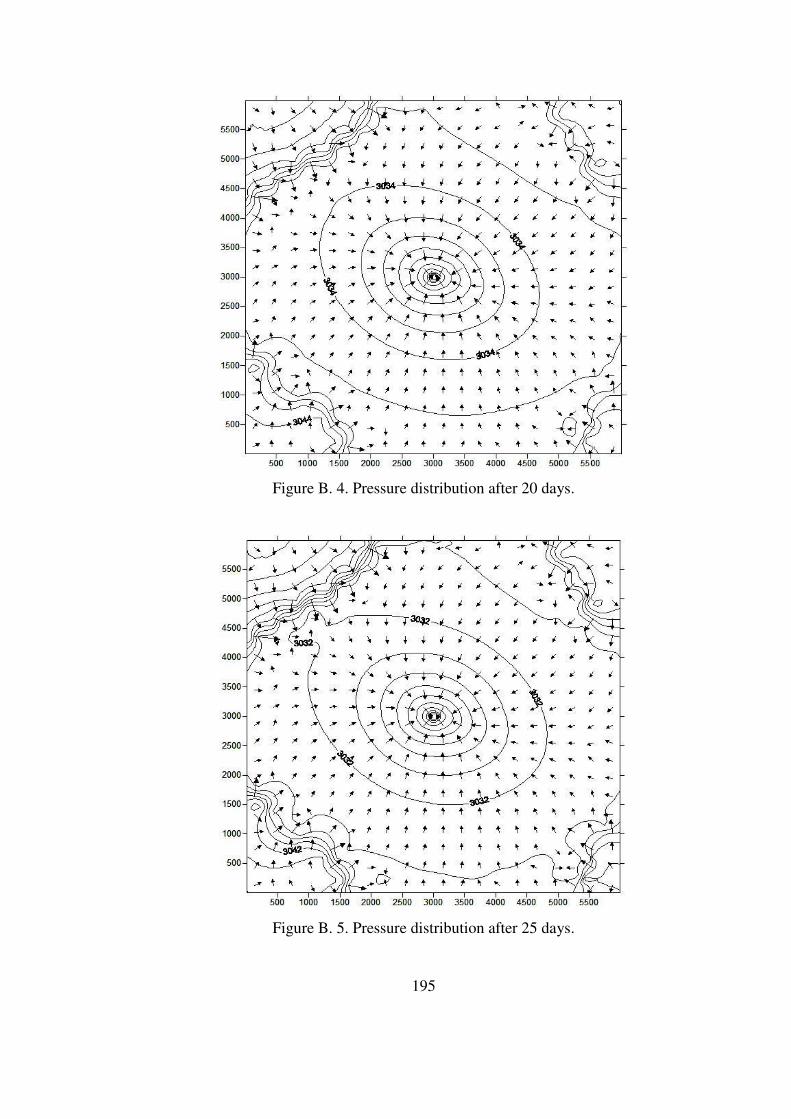
195
Figure B. 4. Pressure distribution after 20 days.
Figure B. 5. Pressure distribution after 25 days.
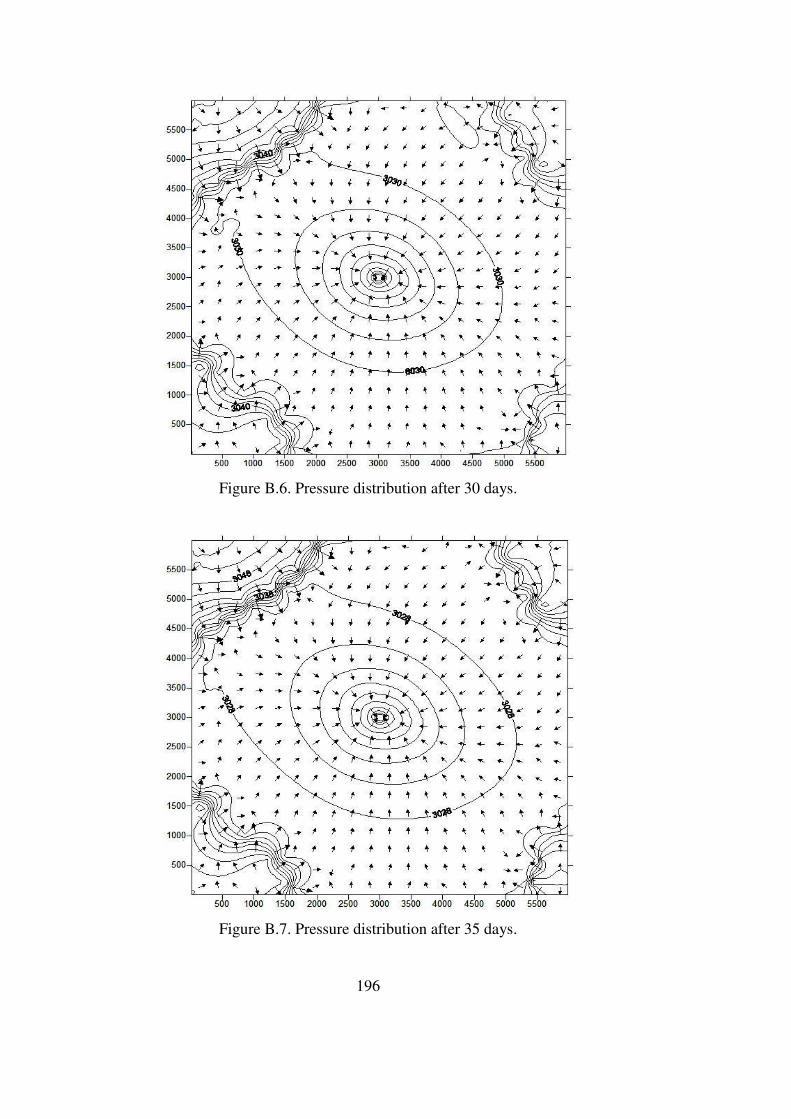
196
Figure B.6. Pressure distribution after 30 days.
Figure B.7. Pressure distribution after 35 days.
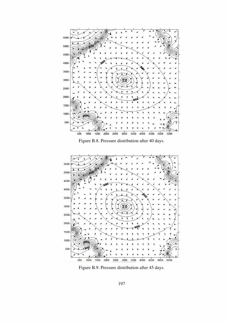
197
Figure B.8. Pressure distribution after 40 days.
Figure B.9. Pressure distribution after 45 days.

198
Figure B.10. Pressure distribution after 50 days.

199
APPENDIX C
CASE 3 FLUID FLOW SIMULATION RUN
This appendix includes fluid flow simulation run for case #3. Inputs for fluid flow
simulation run were grid blocks and permeabilities discussed in sub-chapter 8.2.3,
one vertical well in the middle of reservoir producing at 100 stb/d for 50 days. Initial
reservoir pressure was chosen to be 3044 PSI. Timestep was chosen as 5 days, so
there are 10 pictures showing propagation of pressure disturbance after 5, 10, 15, 20,
25, 30, 35, 40, 45 and 50 days.
Figure C.1. Pressure distribution after 5 days.

200
Figure C.2. Pressure distribution after 10 days.
Figure C.3. Pressure distribution after 15 days.

201
Figure C.4. Pressure distribution after 20 days.
Figure C.5. Pressure distribution after 25 days.

202
Figure C.6. Pressure distribution after 30 days.
Figure C.7. Pressure distribution after 35 days.

203
Figure C.8. Pressure distribution after 40 days.
Figure C.9. Pressure distribution after 45 days.

204
Figure C.10. Pressure distribution after 50 days.

205
APPENDIX D
CASE 4 FLUID FLOW SIMULATION RUN
This appendix includes fluid flow simulation run for case #4. Inputs for fluid flow
simulation run were grid blocks and permeabilities discussed in sub-chapter 8.2.4,
one vertical well in the middle of reservoir producing at 100 stb/d for 50 days. Initial
reservoir pressure was chosen to be 3044 PSI. Timestep was chosen as 5 days, so
there are 10 pictures showing propagation of pressure disturbance after 5, 10, 15, 20,
25, 30, 35, 40, 45 and 50 days.
Figure D.1. Pressure distribution after 5 days.

206
Figure D.2. Pressure distribution after 10 days.
Figure D.3. Pressure distribution after 15 days.

207
Figure D.4. Pressure distribution after 20 days.
Figure D.5. Pressure distribution after 25 days.

208
Figure D.6. Pressure distribution after 30 days.
Figure D.7. Pressure distribution after 35 days.

209
Figure D.8. Pressure distribution after 40 days.
Figure D.9. Pressure distribution after 45 days.
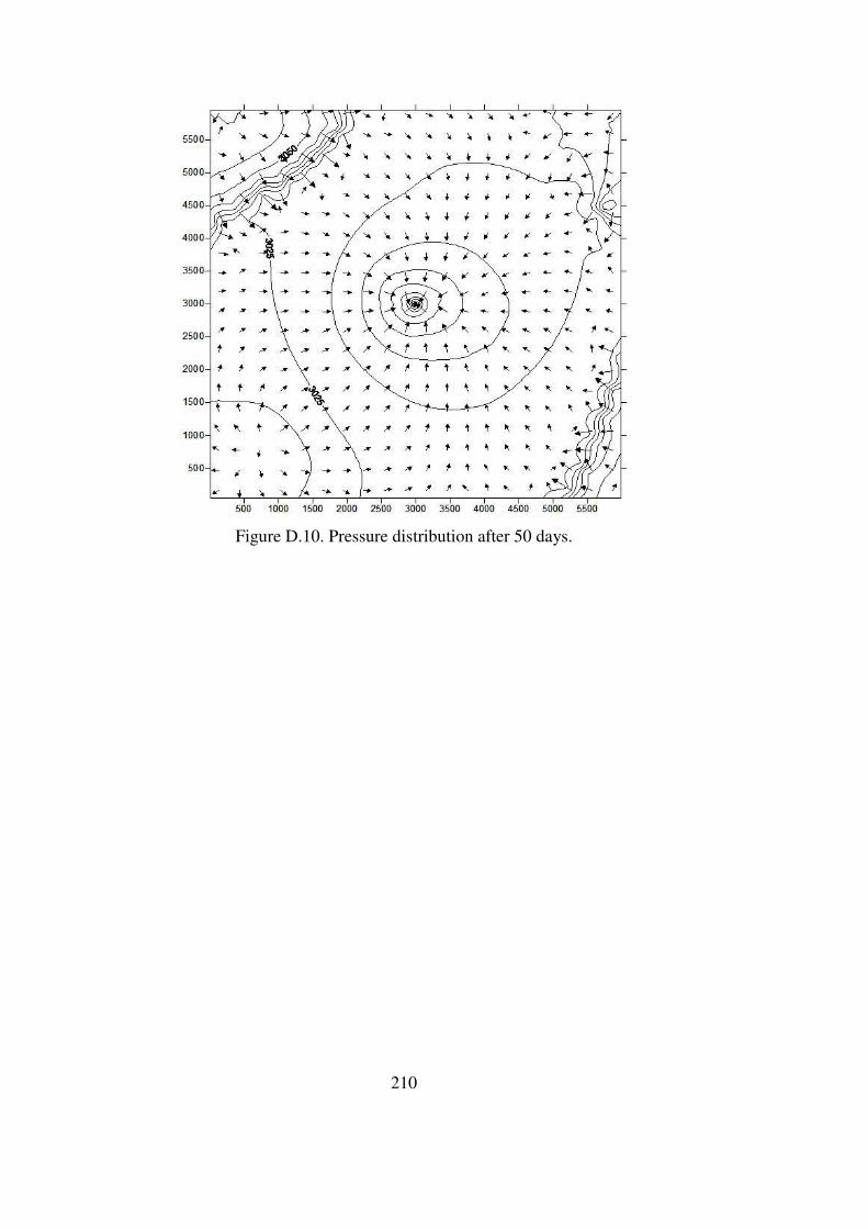
210
Figure D.10. Pressure distribution after 50 days.

211
APPENDIX E
CASE 5 FLUID FLOW SIMULATION RUN
This appendix includes fluid flow simulation run for case #5. Inputs for fluid flow
simulation run were grid blocks and permeabilities discussed in sub-chapter 8.2.5,
one vertical well in the middle of reservoir producing at 100 stb/d for 5 days. Initial
reservoir pressure was chosen to be 3044 PSI. Timestep was chosen as 0.5 days, so
there are 10 pictures showing propagation of pressure disturbance after 0.5, 1, 1.5, 2,
2.5, 3, 3.5, 4, 4.5 and 5 days.
Figure E.1. Pressure distribution after 0.5 days.
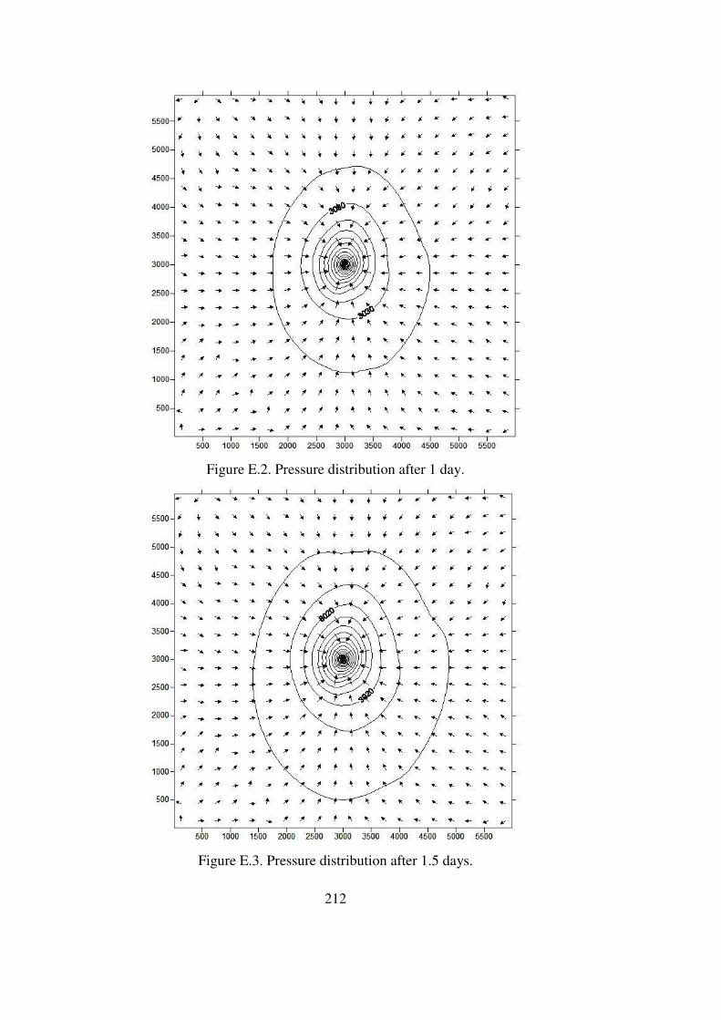
212
Figure E.2. Pressure distribution after 1 day.
Figure E.3. Pressure distribution after 1.5 days.
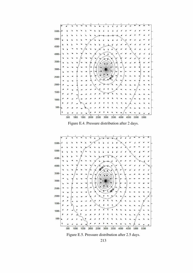
213
Figure E.4. Pressure distribution after 2 days.
Figure E.5. Pressure distribution after 2.5 days.
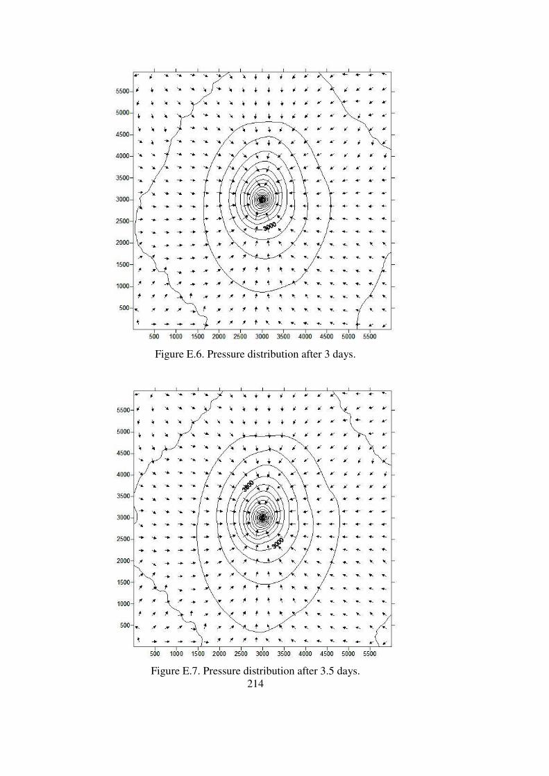
214
Figure E.6. Pressure distribution after 3 days.
Figure E.7. Pressure distribution after 3.5 days.

215
Figure E.8. Pressure distribution after 4 days.
Figure E.9. Pressure distribution after 4.5 days.

216
Figure E.10. Pressure distribution after 5 days.