Optimization models for empty railcar distribution ...cj82k765s/...Optimization Models for Empty...
169
Optimization Models for Empty Railcar Distribution Planning in Capacitated Networks A Dissertation Presented By Ruhollah Heydari to The Department of Mechanical and Industrial Engineering in partial fulfillment of the requirements for the degree of Doctor of Philosophy in the field of Industrial Engineering Northeastern University Boston, Massachusetts January 2016
Transcript of Optimization models for empty railcar distribution ...cj82k765s/...Optimization Models for Empty...

Optimization Models for Empty Railcar Distribution Planning in
Capacitated Networks
A Dissertation Presented
By
Ruhollah Heydari
to
The Department of Mechanical and Industrial Engineering
in partial fulfillment of the requirements
for the degree of
Doctor of Philosophy
in the field of
Industrial Engineering
Northeastern University
Boston, Massachusetts
January 2016
II
ABSTRACT
Because of spatial and temporal imbalances in the supply and demand of empty
railcars/cars in freight transportation systems, empty equipment repositioning is inevitable.
As the owners of rail network, trains and railcars, railway carriers charge their customers
based on the days and the miles that a railcar is under load. Hence the cost of shipping
empty cars to customers as well as the opportunity cost of extra inventory in customer
facilities is on the railway’s shoulder. A reverse routing strategy suggesting to return the
empty cars to the place they were loaded, imposes a 50% empty movement in a car cycle
while a reload strategy suggesting to reload the cars at the point they become empty has
0% empty movement. The first strategy is good for frequent shippers only and still is too
costly and the idealistic second strategy is not usually feasible because of the supply-
demand imbalances. In this research we develop two formulations for the Empty Railcar
Distribution problem, both aiming to minimize the total setup costs, total transportation
costs, and total shortage penalties under supply limitation, demand satisfaction, customer
preferences and priorities, and network capacity constraints.
We first formulate the problem as a path-based capacitated network flow model.
Contrary to the traditional path-based formulations, the path connecting each supply-
demand pair is given by an external application called Trip Planner which is defined on top
of a time-space network. Another application called Pseudo Path Generator then generates
alternative paths for each supply-order pair.
Then we formulate the problem as an arc-based capacitated multi-commodity
network flow model where contrary to the path-based model, the car routing and car
distribution decisions are integrated in a single model.
The path-based formulation is more practical for the United States railroads since
in US railroad industry car routing and car distribution decisions are separated from each
other and usually made by different departments while the integrated arc-based formulation
is close to the Swedish Railway System. Both models are complex and because of the huge
number of constraints and integer decision variables are hard to solve.
The models are implemented in Java and solved using Concert Technology of the
IBM CPLEX solver. We also develop an Iterative Relaxation and Rounding Heuristic using
Initial Basis for the path-based model. The comparison of path-based and arc-based
formulations in both capacitated and uncapacitated modes confirmed the efficiency of the
heuristic from both run time and solution quality perspectives.

III
ACKNOWLEDGEMENTS
I express my sincere gratitude and appreciation to my PhD advisor, Prof.
Melachrinoudis of Northeastern University, for his encouragement, guidance, and
continuous support over the years of my graduate studies, not only in research but also in
other aspects of student life in the United States.
I thank Dr. Kubat and Dr. Turkcan from Northeastern University and Dr. Pranoto
from Norfolk Southern Railway for being part of my PhD committee and providing me
with their valuable comments on this research.
I would also like to thank Dr. Clark Cheng of Norfolk Southern for encouraging
me to choose my Dissertation topic in the area of Car Distribution Problems; Fabio
Colombo from Universita degli Studi di Milano, Italia (Team OR at UNIMI) for providing
me with their group's 2011 RAS competition results; Nilay Roy from Research Computing
Center of Northeastern University for his hours of technical support on distributed
computing; Lisa O'Neill, Director of Graduate Student Services, for her endless support
throughout my educational life at Northeastern University, and all other faculty, staff and
friends who were always there when I needed their support.
I am indebted to my family for their relentless support and encouragement, during
my graduate studies. And I want to express my greatest gratitude to them and specially to
my mom whose patience, love, and praying has always been with me. Finally I will
dedicate this work to my mom. Thank you maman!

IV
LIST OF TABLES
Table 2-1 A comparison among current models used by railway carriers and our model ............. 25
Table 3-1 Parameters used to calculate the cost coefficients ......................................................... 49
Table 3-2 Demand node priorities based on customer priorities ................................................... 49
Table 3-3 Illustration of customer profiles .................................................................................... 51
Table 3-4 Model assumptions ........................................................................................................ 55
Table 4-1 Mathematical notation ................................................................................................... 58
Table 5-1 Notation for the arc-based formulation ......................................................................... 96
Table 5-2 Permitted flows vs leak in the customer level ............................................................... 99
Table 6-1 Networks used for verification and validation of the models and the solution procedures
..................................................................................................................................................... 113
Table 6-2 Customers’ demand for a one-week time horizon ....................................................... 118
Table 6-3 Available supply of different pools in each yard ......................................................... 119
Table 6-4 Performance measures (optimal assigned cars; optimal objective value) for different
models for two scenarios with different shortage penalties ......................................................... 128
Table 6-5 Different models, variable setup and algorithms to solve them .................................. 129
Table 6-6 Parameters used to generate case example for sensitivity analysis ............................. 135
Table 6-7 Parameters used to generate case examples for computational complexity calculations
..................................................................................................................................................... 143

V
LIST OF FIGURES
Figure 3-1 An itinerary for a flight trip .......................................................................................... 27
Figure 3-2 Underlying networks used in the railroad optimization models ................................... 33
Figure 3-3 The time-space network (a) and its associated multigraph (b) ..................................... 37
Figure 3-4 Time-space block-train network associated to Figure 3-2(f) ....................................... 38
Figure 3-5 Time-space resource-constrained block network (colors for visualization) ................. 41
Figure 3-6 Time-space resource-constrained block network (the main representation) ................ 42
Figure 3-7 Customers on time-space resource-constrained block network .................................. 43
Figure 3-8 Bipartite supply-demand multigraph ............................................................................ 44
Figure 3-9 Costs on the time space network .................................................................................. 49
Figure 3-10 Classifying fleet for empty railcar distribution .......................................................... 54
Figure 4-1 Shortage cost function .................................................................................................. 62
Figure 4-2 Car distribution model in three different modes .......................................................... 64
Figure 4-3 An arc-train network with only one path between any O-D pair (a-1) can be
transformed to a resource-constrained bipartite graph (a-2), while the one with more than one
path (b-1) is transformed to a bipartite multigraph (b-2). .............................................................. 68
Figure 4-4 Lattice path of length four in in ℤ𝟐 .............................................................................. 70
Figure 4-5 Six lattice paths and their associated permutation words ............................................ 71
Figure 4-6. A trip plan and its associated pseudo paths when a) no delay is permitted, and b) a
maximum delay of two days is acceptable ..................................................................................... 75
Figure 5-1 Delay arcs in the customer level .................................................................................. 98
Figure 5-2 Permitted flow vs leak in customer level ..................................................................... 99
Figure 5-3 Dealing with delay arc flow using a new variable ..................................................... 101
Figure 6-1 Static networks associated with the Tiny and Supper Tiny Networks: a) physical rail
network, b) train network, c) blocking plan and d) block to train assignment ............................. 113
Figure 6-2 Static networks associated with the Medium Network: a) physical rail network, b)
train network and c) blocking plan .............................................................................................. 114
Figure 6-3 Static networks associated with the Large Network: a) Physical rail network, b) train
network and c) blocking plan ....................................................................................................... 115
Figure 6-4 Detailed supply-order assignment suggested by PA with a) low shortage and b) high
shortage penalties ......................................................................................................................... 123
Figure 6-5 Detailed supply-order assignment suggested by AT with a) low shortage and b) high
shortage penalties ......................................................................................................................... 124
Figure 6-6 Detailed supply-order assignment suggested by NC with a) low shortage and b) high
shortage penalties ......................................................................................................................... 125

VI
Figure 6-7 Detailed supply-order assignment suggested by NCActual with a) low shortage and b)
high shortage penalties ................................................................................................................. 126
Figure 6-8 Optimal assignment from noncapacitated model and its optimistic behavior ........... 127
Figure 6-9 Logistic function for creating daily demand .............................................................. 132
Figure 6-10 Path-Based formulation performance measures at the termination time when capacity
increases: a) objective value, b) order fulfillment, and c) run time ............................................. 139
Figure 6-11 Path-Based formulation performance measures at the termination time when shortage
penalties increase: a) objective value, b) order fulfillment, and c) run time ................................ 142
Figure 6-12 Average solution time of AT-IRRH2 with initial basis (solid green circles) along with
its estimation from the regression model (empty blue circles) .................................................... 144
Figure 6-13 Average run time vs estimated run time from a power law model .......................... 145
Figure 6-14 The performance measures of IRRH2 per iteration when the problem size increases.
a) EpGap, b) solution time, and c) their trade-off ........................................................................ 147

VII
TABLE OF CONTENTS
1 Introduction ...................................................................................................................1
1.1 Problem Background ........................................................................................................ 1
1.2 Problem Statement .......................................................................................................... 2
1.3 Motivation and Objectives of the Dissertation ................................................................ 3
1.4 Dissertation Outline ......................................................................................................... 6
2 Literature Review ...........................................................................................................8
2.1 Transportation Problem ................................................................................................. 11
2.2 Transshipment and Network Flow Problem .................................................................. 13
2.3 Multi Commodity Network Flow Problem ..................................................................... 18
2.4 Economies of Scale ........................................................................................................ 20
2.5 Survey Papers ................................................................................................................. 22
2.6 Contribution of the Research ......................................................................................... 22
3 Important Terminologies and Components of the Problem ............................................ 26
3.1 Important Terminologies ............................................................................................... 26
3.2 Network Representation ................................................................................................ 29
3.2.1 Static Networks ...................................................................................................... 29
3.2.2 The Time-Space Network ....................................................................................... 35
3.2.3 The Bipartite Multigraph ........................................................................................ 44
3.2.4 Network Capacities ................................................................................................ 45
3.2.5 Cost Components ................................................................................................... 45
3.3 Fleet ............................................................................................................................... 50
3.4 Customer, Customer profile, Demand node and Demand ............................................ 50
3.5 Supply ............................................................................................................................. 52
3.6 General Assumptions on the Components of the Model .............................................. 55
4 Path-Based Formulation for Car Distribution Problem ................................................... 56
VIII
4.1 A General Integer Programming Formulation ............................................................... 56
4.2 Pure Allocation Model on a Bipartite Resource Constrained Graph ............................. 65
4.3 Allocation-Timing Model on a Bipartite Resource Constrained Multigraph ................. 69
4.3.1 An Algorithm for Generating Pseudo-paths of a Trip plan .................................... 69
4.3.2 A Lagrangian Heuristic ........................................................................................... 76
4.3.3 An Iterative Relaxation and Rounding Heuristic .................................................... 83
4.4 Noncapacitated Model and its Optimistic Behavior on a Capacitated Network ........... 86
4.5 Trip Planning Algorithm ................................................................................................. 91
4.5.1 Trip Planning on the Time-Space Block-Train Network ......................................... 92
4.5.2 Trip Planning on the Time-Space Resource Constrained Blocking Network ......... 93
5 Arc-Based Formulation for the Car Distribution Problem ............................................... 94
5.1 Allocation-Routing Model .............................................................................................. 94
5.2 Formulating the Anti-Leak Rule using Extra Constraints ............................................. 100
5.3 Formulating the Anti-Leak Rule with Redefining the Decision Variables .................... 100
6 Numerical Results ....................................................................................................... 105
6.1 Verification and Validation .......................................................................................... 107
6.2 Illustrative Example ...................................................................................................... 116
6.2.1 Input data ............................................................................................................. 116
6.2.2 Model Results, Interpretation, and Remarks ....................................................... 119
6.3 Performance of Models and Solution Procedures in Larger Scale Problems .............. 128
6.3.1 Generating case examples ................................................................................... 130
6.3.2 Sensitivity Analysis on Network Capacities .......................................................... 134
6.3.3 Sensitivity Analysis on Shortage Penalties ........................................................... 140
6.3.4 Average Time Complexity of the Proposed Heuristic .......................................... 142
6.3.5 Solution Quality of the Proposed Heuristic ......................................................... 146
7 Summary, Results and Future Research ....................................................................... 148
7.1 Summary ...................................................................................................................... 148
7.2 Results .......................................................................................................................... 151
IX
7.3 Future Research ........................................................................................................... 151
References ......................................................................................................................... 153

1.1 Problem Background
1
Chapter 1
1 Introduction
1.1 Problem Background
Freight railroads receive shipment requests from customers (internal or external) to
transport cars. External customers, also referred to as customers, send their empty car
requests to the railroad's car distribution unit. Once a customer asks the car distribution
unit to send one empty railcar to its facility, the car distribution unit will allocate an empty
railcar in the network that is suitable for the customer request and, as an internal customer,
will send a shipment request to the railroad operation department. The operation
department then generates a trip plan indicating the path the car will follow from its origin
to its destination. Once it arrives at the customer facility, the car will be loaded by the
customer. Next, the customer sends a shipment request to the railroad to pull the loaded
car to the destination they determine. The operation department then generates another trip
plan to take this loaded car to its destination. A shipment will have attributes such as origin,
destination, car type, physical dimensions, freight type, etc., which will be used by the trip
planning application to generate the trip plan for this shipment. Once it arrives at the
destination, the car will be unloaded and the railroad will be notified that the car is empty.
Once the empty car is released by the customer, one car cycle has finished and the car can
be allocated again to other customers by the car distribution unit. In this research we mainly

1.2 Problem Statement
2
focus on the part of the decision that is made by the car distribution unit of the railroad in
allocating empty railcars, supply, to customer order, demand.
1.2 Problem Statement
This research primarily deals with developing effective models for the distribution
of empty railcars in order to fulfill customer demand over a multi-period horizon, under
the constraints of supply and demand and network capacities. Furthermore, the research
will address various issues including customer priorities, order expiration dates, and
permitted substitutions. Also, since the car distribution problem is an operational decision,
suitable real-time solution methods will be developed and validated in order to be useful
to the railroad carriers.
Although in the literature the words distribution, allocation, repositioning, and
assignment are used interchangeably to address this problem, even if it is combined with
other optimization problems, e.g. with car routing problem, we will slightly differentiate
between these terms in this research. We first use the term "empty car/railcar distribution"
as a general term to refer to the repositioning of empty railcars from supply locations to
demand locations, and then divide car distribution problems into two categories. The first
category covers the pure allocation, or assignment, of supply to demand, where the route
between supply and demand locations, known as a trip plan in railroad language, is given
by an independent application and is out of the scope of the allocation model. The second
category, however, simultaneously covers both the allocation of empty cars to the demand
for cars and their associated routings in an integrated allocation-routing model. Clearly, the
aggregated decision from the optimal car routing and car allocation problems might be sub-
optimal compared to the one achieved from the integrated allocation-routing model.

1.3 Motivation and Objectives of the Dissertation
3
However, the integration of allocation and routing decisions might not be applicable to all
railroads as the decision makers might be different. Whether the first or the second
modeling category is suitable for a certain railroad depends on the organization and the
policies of that railroad. For example, U. S. Class 1 railroads, currently separate the car
allocation and car routing decisions (Gorman et al., 2011), while Swedish National
Railroad combines them (Holmberg et al., 1998).
1.3 Motivation and Objectives of the Dissertation
Because of spatial imbalances in the supply and demand of empty railcars in the
freight transportation system, empty equipment repositioning is inevitable. Historically,
railroads have used different repositioning methods, including dedicated pools (where a
car is dedicated to a customer and will be returned to the same customer once it becomes
empty), single-car allocation (ad hoc rules of assigning empty cars to customers; for
example, supply covered coil demand of Pennsylvania from Conway Hub), offline
optimization models (optimizing the assignment of projected supply and forecasted
demand, as in old CSX Sentinel system), and most recently, real time optimization models,
implemented by railway carriers CSX, BNSF, UP and CP (Gorman et al., 2010).
In 1997, CSX implemented their real-time car distribution system, Dynamic Car
Planning (DCP), formulated as a single commodity network flow problem which was
solved using a proprietary LP algorithm. By investing $5 million in DCP, CSX has claimed
a reduction of 7% in empty railcar movement, translated into annual savings of $50 million
(Gorman et al., 2010).
In 2000, BNSF launched their real-time car distribution system, Equipment
Distribution Optimization (EDO), which is formulated as a transportation problem. BNSF

1.3 Motivation and Objectives of the Dissertation
4
reported an annual savings of $13 million after installing this $3 million system (Gorman
et al., 2011).
Another North American Class 1 Railroad, UP has reported 35% ROI by reducing
manpower needed for the demand fulfillment process and a significant reduction of costs
by allowing the carrier to manage the cost of the miles moved while meeting the delivery
date for empty cars. (Narisetty et al., 2008).
In Europe, the European Commission (EC) has funded a number of research works,
among them the WagonLink (railcar reservation system), CroBIT (data exchange platform)
and F-MAN (real-time track-and-trace and railcar management) projects in order to
investigate the deficiencies of the railcar management system and propose solutions for its
advancement (Ballis and Dimitriou, 2010). Also Swedish State Railway has developed the
kernel of their empty railcar distribution system based on a multi-commodity network flow
model presented by Holmberg et al. (1998).
Despite the vast studies performed in the railroad optimization modeling, there is
still a need for another realistic modeling and optimization of the empty railcar distribution
problem. In particular, there is no previous work that optimizes the empty railcar
distribution decisions while simultaneously considering the resource (capacity)
availabilities in the service network and the car type substitutability for the customer
demands as well as separating the car distribution and car routing decision in accordance
to the US railroad practices.
Current practices of the U. S. railroads do not consider network capacities in car
allocation or in trip planning models. Ignoring capacity limits on the network will make
the allocation and routing decisions independent of each other. This by itself justifies why

1.3 Motivation and Objectives of the Dissertation
5
these decisions are currently separated from each other in the U.S. railroads. However,
formulating the problem as a classical transportation model, or as an uncapacitated
minimum cost flow formulation, might deliver solutions that are practically infeasible or
feasible with higher costs in the real application under the presence of the network
capacities. A capacitated multi-commodity network flow formulation, used for the Swedish
National Railway, is also not fully applicable to the U.S. railroads mainly because it
combines car routings and car distribution decisions.
The situation in US railroads is changing however. As presented in INFORMS
(https://www.informs.org/content/ download/239255/2274025/ .../SC1.pdf), Norfolk
Southern's Next Generation car routing system (ABC-NG) will consider network capacities
(block capacities and train capacities) while creating the trip plans. Once network
capacities are considered in the trip plan application, considering them in the allocation
model seems inevitable. It is noteworthy that one of the principal causes of uncertainty in
the travelling time arises from ignoring the network capacities in both the car allocation
and the car routing decision making processes. By formulating the problem on a
capacitated network, we can decrease the level of uncertainty in travel times, and as a result
construct a deterministic model. Furthermore once capacities are considered during car
routing and car distribution decision making, integrating empty car allocation and car
routing decision could be the next logical step to lower the railroad operational costs. This
is the reason we build our car distribution model, complying with current organization of
US railroad which separates the car distribution and car routing decisions, on top of a
capacitated network and compare its performance with both noncapacitated model and an
integrated allocation-routing model. The objective of this research can be summarized as:
1.4 Dissertation Outline
6
to develop realistic optimization models for the distribution of empty
railcars and
to develop effective solution methods for solving those models and finally
to validate the accuracy of the developed models and to verify the accuracy
of computer programs developed for those models using verification and
validation techniques
1.4 Dissertation Outline
The Dissertation is organized as follows. In Chapter 2 the literature of empty railcar
distribution problem is studied, from both practical and theoretical perspectives. The
previous research is classified in three categories based on the formulation: Transportation
problem, Transshipment and network flow, and multi commodity network flows. At the
end of Chapter 2, the gap between the literature and the reality is identified and the
contribution of this research is described.
Important terminologies, vastly used in the future chapters, as well as the
components of the input data set are described in Chapter 3 before presenting car
distribution models in Chapter 4 and 5.
A path-based formulation for the capacitated car distribution problem is presented
in Chapter 4 in two different modes: mode 1) The pure allocation, or simply the allocation
model, where each feasible supply-demand pair is connected using only one path; and
mode 2) the allocation-timing model, where more than one path is allowed between them.
A third formulation where all feasible paths are considered can be transformed to an arc-
based formulation and is discussed in Chapter 5.

1.4 Dissertation Outline
7
The arc-based formulation presented in Chapter 5 is defined on a time-space
network and integrates car routing and car distribution decisions in a single Allocation-
Routing model.
The numerical techniques and results are presented in Chapter 6. First the
verification and validation techniques are described then the implementation of the path-
based and arc-based formulations of the car distribution problem is illustrated in a small
size example on a medium size network and finally the average time complexity of the
developed heuristics is calculated by generating random problem instances of various sizes.

1.4 Dissertation Outline
8
Chapter 2
2 Literature Review
The empty car distribution problem has been studied for half a century from both a
theoretical and a practical perspective. Dejax and Crainic (1987) describe several criteria
that might be used to classify the numerous works that appeared in the literature of the
empty flow and fleet sizing models. In this section we slightly redefine those criteria to be
suitable for the empty car distribution problem.
Problem statement criteria:
Optimization focus or the level of integration: in a pure car allocation model the decision
made is car-to-order assignments only (Gorman et al., 2010, 2011). Other optimization
problems such as car routing and train and crew scheduling are optimized in different
applications. In an integrated car distribution model however, car allocation might be
integrated with other optimization problems. For example, it can be integrated with the car
routing problem and be formulated as a transshipment problem (Holmberg et al., 1998). Or
it can be integrated with the train routing problem (Haghani, 1989).
Fleet homogeneity: in a homogeneous fleet (case of the single commodity problem) all
cars are eligible to be allocated to all orders. In a heterogeneous fleet (case of the multi-
commodity problem), there are several types of cars that might be partially or totally

1.4 Dissertation Outline
9
substituted for each other. It is noteworthy that if the heterogeneous fleet can be divided
into multiple groups that cannot be substituted for each other like tank cars and coil cars
and if cars in different groups do not share resources with each other like in uncapacitated
networks, then the problem can be decomposed to multiple homogeneous fleet sub-
problems (Holmberg et al., 1998).
Transportation mode: while container management and intermodal transportations has
been studied vastly (Choong et al., 2002; Wang and Wang, 2007; Dong and Song, 2009;
Dang et al., 2012; Song and Dong, 2013), in this research we will focus on rail cars only
and will not study intermodal car distribution case.
Type of flow: while most of car distribution problems focus on the empty flow only, there
are some problems that consider both empty and load movements (Bandeira et al., 2009;
Mesa-Arango et al., 2013).
Modeling assumptions criteria:
Time domain: some researchers consider only static cases (Misra, 1972), while some
others take time into consideration and formulate the problem as a dynamic model (White,
1972; Jordan and Turnquist, 1983; Powell, 1987; Godfrey and Powell, 2002).
Level of certainty: some researchers treat the problem as a deterministic problem and
perform frequent runs to overcome the dynamics of data (Gorman et al., 2010, 2011), while
others exclusively consider the stochasticity of supply, demand or network data as part of
formulation (Jordan and Turnquist, 1983; Topaloglu and Powell, 2005; Powell and
Topaloglu, 2006; Topaloglu and Powell, 2006; Lam et al., 2007; Topaloglu, 2007; Cao et
al., 2008; Erera et al., 2009).

1.4 Dissertation Outline
10
Side constraints: in addition to the supply and demand constraint, a car distribution
problem might have some side constraint, for example network capacity constraints
(Holmberg et al., 1998).
Problem formulation criteria:
Single objective or multi objective: while minimizing the total allocation cost is the most
common objective in the literature, some researchers have considered other objectives, e.g.
minimizing the total tardiness (Spieckermann and Voß, 1995).
Modeling technique: different researchers has used different techniques such as : general
mathematical models (LP, IP, MLP, MIP, etc.), network models, simulation models or
stochastic models to formulate the car distribution problem.
Solution criteria:
Solution precision: Exact algorithms (e.g. network algorithms or simplex algorithm) were
used when the problem size was small (Misra, 1972) or the model was simplified, by for
example relaxing the capacities, to make it practical for real word implementations
(Gorman et al., 2011), while heuristics or metaheuristics were developed mainly for the
integrated models when the state-of-the-art software were not able to solve the complex
formulations (Holmberg and Yuan, 2003; Holmberg et al., 2008; Joborn et al., 2004).
Solution validation: some models are tested on the real world networks as case studies.
For example Sherali and Suharko (1998) uses TTX data to validate their model and
Spieckermann and VoB uses CARGOWAGGON GmbH of Germany for validation
purposes. Some other works are published results of the real world implementation of the

2.1 Transportation Problem
11
models (Holmberg et al., 1998; Narisetty et al., 2008; Gorman et al., 2010, 2011; Engels,
2011). The majority of the works however, discuss the theory of the car distribution
problem.
From a modeling perspective, the problem has been mostly formulated as a
transportation problem, pure or with side constraints, network flow problem (for example
transshipment problem, pure or with side constraints) and with multi commodity flows. In
the next section, we review these models as well as the relevant literature of the empty
railcar distribution.
2.1 Transportation Problem
The transportation problem was formulated first by Hitchcock in 1941 and then
independently by Koopmans in 1951, and it is therefore also referred to as the Hitchcock-
Koopmans problem.
The problem is defined over a bipartite graph of supply nodes on one side and
demand nodes on the other side and seeks the optimal distribution plan of units of a single
product from supply points 𝑖 ∈ 𝐼 to demand points 𝑗 ∈ 𝐽 while minimizing the total
transportation cost.
Let 𝑠𝑖 be the amount of supply at a supply node 𝑖 ∈ 𝐼 and 𝑑𝑗 be the demand at a
demand node 𝑗 ∈ 𝐽. Also, let 𝑐𝑖𝑗 and 𝑥𝑖𝑗 be the unit transportation cost between 𝑖 and 𝑗, and
the amount transported between these nodes, respectively. The mathematical programming
of the transportation problem then is given as:
𝑀𝑖𝑛 ∑ ∑ 𝑐𝑖𝑗𝑥𝑖𝑗𝑖∈𝐼𝑗∈𝐽 (2-1)
Subject to:
2.1 Transportation Problem
12
∑ 𝑥𝑖𝑗𝑗∈𝑗 = 𝑠𝑖 ∀𝑖 ∈ 𝐼 (2-2)
∑ 𝑥𝑖𝑗𝑖∈𝐼 = 𝑑𝑗 ∀𝑗 ∈ 𝐽 (2-3)
𝑥𝑖𝑗 ≥ 0 𝑖 ∈ 𝐼, 𝑗 ∈ 𝐽 (2-4)
The objective function (2-1) minimizes the total transportation cost. The constraint
set (2-2) stipulates that the total shipments from a node must be equal to its supply;
similarly, the constraint set (2-3) states that the total shipments to a demand node must
satisfy its demand. Finally constraint set (2-4) prevents negative flows in the network. In
order to guarantee the feasibility of this model, total supply must be equal to total demand,
i.e. ∑ 𝑠𝑖𝑖∈𝐼 = ∑ 𝑑𝑗𝑗∈𝐽 .
Several algorithms have been developed to solve this problem including but not
limited to the one by Hitchcock himself, and those by Dantzig (1951), and Ford and
Fulkerson (1956). In textbooks however, the problem is solved by a version of simplex
method called transportation simplex.
One important feature of the transportation problem (and in general any network
flow problem) is the unimodularity of the constraints' coefficient matrix. As a result, if the
supply and demand quantities, i.e. right hand sides, are integers, then the optimal solution
will also be integer valued, in other words in order to solve the integral transportation
problem, it is sufficient to solve the LP relaxation of the problem. This characteristic along
with the easy formulation of the problem has motivated many researchers and practitioners
to use transportation model in the empty railcar distribution formulations.
Misra's (1972) article was the first published work that formulated the problem as
a transportation model minimizing the total travel time over a static time period. He
proposed transportation simplex as a solution method. In the same paper, he also covered

2.2 Transshipment and Network Flow Problem
13
the capacitated model, where some arcs of the rail network, called bottlenecks, have
capacity limitations. His capacitated model integrates the car allocation and routing
together and is solved by the simplex method. Sherali and Suharko (1998) presented two
formulations for the problem of repositioning TTX cars, one of which is a capacitated
transportation model. A detailed discussion on the cost function formulation of their model
is presented in Suharko (1997). Their second model considers economies of scale and will
be discussed later. While transportation problem formulation seems too simple to be used
by the railroads, it has actually been deployed in practice. In 2000, BNSF launched their
real-time car distribution system, Equipment Distribution Optimization (EDO), which is
formulated as a transportation problem. BNSF reported an annual savings of $13 million
after installing this $3 million system (Gorman et al., 2011).
2.2 Transshipment and Network Flow Problem
The objective of a minimum cost network flow problem is to determine the least
cost shipment of a commodity through a network in order to satisfy demands at certain
nodes from available supplies at other nodes. Unlike the transportation problem, the
network here is not necessarily a bipartite graph. In fact, the transportation problem is a
special case of the minimum cost flow problem.
Let 𝐺(𝑉, 𝐸) be a finite, connected, directed and weighted network with node
set 𝑉 of 𝑛 nodes and edge set 𝐸 of 𝑚 directed arcs. Associated with each arc (𝑖, 𝑗) ∈ 𝐸
there is a cost 𝑐𝑖𝑗 representing the cost per unit flow on that arc as well as two bounds, 𝑙𝑖𝑗
and 𝑢𝑖𝑗, respectively representing the minimum and maximum amount that can flow on the
arc. Each node 𝑖 ∈ 𝑉 has an integer weight 𝑏𝑖 representing its supply/demand. If 𝑏𝑖 > 0,
node 𝑖 is a supply node; if 𝑏𝑖 < 0, node 𝑖 is a demand node with a demand of −𝑏𝑖; and if

2.2 Transshipment and Network Flow Problem
14
𝑏𝑖 = 0, node 𝑖 is a transshipment node. The decision variables in the minimum cost flow
problem are arc flows represented by 𝑥𝑖𝑗. The mathematical formulation of the problem is
as follows (Ahuja et al., 1993):
𝑀𝑖𝑛 ∑ 𝑐𝑖𝑗𝑥𝑖𝑗(𝑖,𝑗)∈𝐸 (2-5)
s.t.
∑ 𝑥𝑖𝑗{𝑗:(𝑖,𝑗)∈𝐸} − ∑ 𝑥𝑗𝑖{𝑗:(𝑗,𝑖)∈𝐸} = 𝑏𝑖, ∀𝑖 ∈ 𝑉, (2-6)
𝑙𝑖𝑗 ≤ 𝑥𝑖𝑗 ≤ 𝑢𝑖𝑗 , ∀(𝑖, 𝑗) ∈ 𝐸, (2-7)
where ∑ 𝑏𝑖𝑛𝑖=1 = 0. A matrix representation of the problem is as follows:
𝑀𝑖𝑛 𝑐𝑥 (2-8)
s.t.
𝐴𝑥 = 𝑏, (2-9)
𝑙 ≤ 𝑥 ≤ 𝑢, (2-10)
where 𝐴 is an 𝑛 × 𝑚 matrix, called the node-arc incidence matrix of the minimum cost
flow problem. It is proven that the node-arc incidence matrix of the network flow problem
is totally unimodular and therefore unimodular and as a result, every basic feasible solution
of the problem is an integer for any integer vector 𝑏.
The constraints in set (2-9) are known as mass balance constraints. The mass
balance constraint states that the outflow (i.e., the flow emanating from the node) minus
the inflow (i.e., the flow entering the node) must equal the supply/demand of the node. If
the node is a supply node, its outflow exceeds its inflow; if the node is a demand node, its
inflow exceeds its outflow; and if the node is a transshipment node, its outflow equals its

2.2 Transshipment and Network Flow Problem
15
inflow. The flow must also satisfy the lower bound and capacity constraints (2-10), which
are referred to as flow bound constraints. A minimum cost flow model without any
constraint on arc flow bounds is called a transshipment model.
As stated in Ahuja et al. (1993), the minimum cost flow model is the most
fundamental of all network flow problems and is widely used in different applications such
as supply chain management; production lines; call routing through telephone systems, and
empty railcar distribution systems.
The minimum cost flow problems used in empty railcar distributions can be divided
into two categories based on the nature of the transshipment nodes: Those with temporal
transshipment nodes and those with temporal or physical transshipment nodes. In the first
group, cars flowing from supply nodes to demand nodes do not travel through any other
physical node of the network, or at least we can say the model does not deal with the
movements through the intermediate nodes. Transshipment nodes here are not physical
nodes but temporal nodes added to the network to transform, for example, a static
transportation problem (capacitated transportation problem) to a dynamic model
formulated as transshipment problem (minimum cost flow problem). The decision
variables of these models can be easily translated to supply-to-demand assignment
decisions. In fact the operational department will know how many cars, at what time, and
from what supply nodes, are planned to be sent to what demand nodes. The second group
consists of the models in which the flow of cars, from the supply nodes to the demand
nodes, is physically transferred through other nodes of the network. The solution of these
models gives the flow of cars on each arc of the network, but does not explicitly offer any
supply to demand (origin to destination) assignment. In the United State railways, the
2.2 Transshipment and Network Flow Problem
16
origin and destination of each car movement have to be specified as the output of the car
distribution decision. Ahuja et al. (1993) describe an algorithm to decompose the arc flow
solution into path flows. The output of such an algorithm however, suggests that both the
car assignment and the car routing decisions are made at once which is not in alignment
with the US railroad processes and policies that separate these decisions (Gorman et al.,
2011).
The research by White and Bomberault (1969) was the first to formulate the car
distribution problem as a transshipment problem in a time-space network. It was the first
time that dynamics were added to the car distribution model. The arcs of this network
represent the scheduled trains and the nodes stand for the train events, i.e. train departure
and arrivals. The underlying time-space network was called the dynamic transshipment
network three years later in an extension of this paper to the empty container allocation
problem (White, 1972). Each node in the dynamic transshipment network represents a
location in a specific time. Nodes are connected to one another by movement arcs and
inventory arcs. A movement arc (referred to as a physical arc in their work) represents a
movement from one location to another and is associated with a travel cost, while an
inventory arc (referred to as temporal arcs in their work) connects two nodes corresponding
to one location in two consecutive days and is associated with a storage cost. The network
is acyclic and no backward-time arc is allowed. They used an adoption of the out-of-kilter
algorithm to solve their model. White and Bomberault (1969) and White (1972) both
emphasized the importance of car substitution and network capacities in the real world
railroad operations and suggested that these concepts should be studied in future research.
In his Master thesis, Ouimet (1972) studied the capacitated version of White and

2.2 Transshipment and Network Flow Problem
17
Bomberault (1969), which by definition is considered a minimum cost network flow
problem, and suggested an out-of-kilter algorithm to solve it. The fleet however was
considered homogeneous.
Herren (1977) considered another minimum cost flow formulation for the car
distribution problem at the Swiss Federal Railroad (SBB). As the model was built to be
sent to operations, the fleet, this time, was considered heterogeneous with substitution
possibilities and the resulted transshipment problem was solved by a modified out-of-kilter
algorithm. Turnquist and Markowicz (1989) presented a new time-space schema for the
problem. In their model each location in each day is represented by at least three nodes:
one demand node plus one supply node and one collector node for each car type. For
example if there are two car types, each location-time will be represented by five nodes
(one demand node, two supply nodes and two collector nodes. In addition to the supply
and demand nodes and movement and inventory arcs presented in White and Bomberault
(1969), they introduced collector nodes and reverse arcs that enabled them to formulate the
backorder in their model. Using this new network representation, they were able to
formulate the problem with partial substitution as a single commodity network flow
problem. The research was tested and implemented at CSX railroad from 1990 to 1996
(Newman et al., 2002). Then, in 1997, CSX implemented their real-time car distribution
system, Dynamic Car Planning (DCP), formulated as another single commodity network
flow problem which was solved using a proprietary LP algorithm (Gorman et al., 2010).
CSX formulation's underlying network contains four layers of nodes: one source node,
multiple supply nodes, multiple demand nodes, and one sink node, without the introduction
of intermediate nodes between supply and demand nodes. While there is no capacity

2.3 Multi Commodity Network Flow Problem
18
restriction on the arcs, demand nodes have a restricted inflow equal to the customer
demand. This restriction on the inflow of a node is also known as the node capacity. In the
formulation of minimum cost flow problem presented at the beginning of this section,
network arcs are capacitated but there is no restrictions on the node capacities. However
they were still able to use minimum cost flow algorithms to solve the problem, as a node
with a restricted inflow could be replaced by two unrestricted nodes connected by an arc
of the relevant capacity. In their case, such a change is not necessary, as each demand node
has only one single outflow arc and the demand nodes' capacities can be dropped after
enforcing a capacity limit of the same amount to their associated single outflow arcs.
2.3 Multi Commodity Network Flow Problem
The multicommodity flow problem deals with the shipment of several commodities
along the arcs of an underlying network. Depending on the application, the commodities
are either distinguished by their physical characteristics or simply by their origin and
destination nodes. In the empty car distribution problem, where different car types need to
be assigned to different customer demands, the first definition of commodity is a good fit,
while the second type of application can be used in the routing of the loaded cars in
railroads when the origin and the destination of each load is known in advance.
The minimum cost multicommodity flow problem can be formulated as follows
(Ahuja et al., 1993):
𝑀𝑖𝑛 ∑ 𝑐𝑘𝑥𝑘𝑘∈𝐾 (2-11)
s.t.
𝐴𝑥𝑘 = 𝑏𝑘 ∀𝑘 ∈ 𝐾, (2-12)

2.3 Multi Commodity Network Flow Problem
19
∑ 𝑥𝑖𝑗𝑘
𝑘∈𝐾 ≤ 𝑢𝑖𝑗 ∀(𝑖, 𝑗) ∈ 𝐸, (2-13)
0 ≤ 𝑥𝑖𝑗𝑘 ≤ 𝑢𝑖𝑗
𝑘 ∀(𝑖, 𝑗) ∈ 𝐸, ∀𝑘 ∈ 𝐾, (2-14)
where 𝐴 is the node-arc incidence matrix of the network, the decision variable 𝑥𝑖𝑗𝑘
represents the flow of commodity 𝑘 on arc (𝑖, 𝑗), and 𝑥𝑘, 𝑏𝑘 and 𝑐𝑘 represent the flow
vector, the supply/demand amount vector, and per unit cost vector for commodity 𝑘
respectively. Each arc (𝑖, 𝑗) has two sets of capacity constraints: an individual commodity
capacity, 𝑢𝑖𝑗𝑘 , limiting the flow of commodity 𝑘 on the arc and an arc bundle capacity, 𝑢𝑖𝑗 ,
limiting its total flow of all commodities.
A minimum cost multicommodity flow problem seeks the optimal allocation of the
capacity of each arc to the individual commodities while minimizing the overall flow costs
(2-11). Each commodity has its own mass balance constraints (2-12), but the arc capacities
are shared among all commodities (2-13). In some applications, the flow of each commodity
on each arc is also bounded (2-14).
Unlike the single commodity network flows, the integrality of the multicommodity
network flow problems' solution is not guaranteed. It is because the unimodularity of the
constraints coefficient matrix is violated as a side effect of the arc bundle capacities.
The multicommodity flow problem has many practical applications, such as the
transportation of passengers within a city, the transmission of messages in a
communication network between different origin-destination (O-D) pairs and the
distribution of empty (or loaded) cars sharing the same transportation network. The
introduction of this model to the empty railcar distribution problem goes back to the end
of the 20th century.

2.4 Economies of Scale
20
Joborn's (2001) Ph.D. dissertation and Holmberg's et al. (1998) research for the
Swedish National Railway were the first published works that formulated the empty railcar
distribution problem as a multi commodity network flow model. In their model, no
substitution was allowed but different commodities (car types) shared same capacitated
trains (arcs). One approximate solution was to list commodities in an order and to solve a
series of inter-related single commodity problems, where the arc capacities needed to be
updated after running for each commodity. However, in order to find the global optimal
solution they used two methods. The first one was to use a Lagrangian based heuristic and
the second one was to solve by CPLEX package. Joborn et al. (2004) expanded this non-
substitutable multi commodity network flow model by charging fixed costs on origin-
destination pairs to exploit economies of scale that enforce multiple empty cars to be
grouped and sent in large clusters. The detail of their model is presented in Section 2.4.
2.4 Economies of Scale
Increasing the profit by means of lowering the marginal cost of transportation has
been considered in many railroad-related researches. In fact the motivation behind the
block design problem that arises in the tactical level of decision making in the railroad
industries is to gain economies of scale by moving larger numbers of cars in groups rather
than individual cars travelling from their origins to their destinations.
To the best of our knowledge, Turnquist's (1994) technical report was the first
attempt to formulate economies of scale in the car distribution model. He used a time-space
network similar to the one in Turnquist and Markowicz (1989) for his uncapacitated
network design formulation. Economies of scale was gained by charging a fixed cost on
the O-D pairs utilized in the distribution and the objective was to minimize both

2.4 Economies of Scale
21
transportation costs (variable costs) and the number of O-D pairs (fixed costs). His case
study results showed a near 50% improvement in all criteria he listed for the car utilization,
however, with an extremely high cost on execution time. For example the running time for
a network with 4k nodes and 14k arcs, jumped from 1 minute to 14 hours, what he
described as "the operation was successful, but the patient died!". As computer technology
substantially improved from 1994 to 2004, Joborn et al. (2004) extended Turnquist's work,
by adding the capacities on the trains that pull cars from their origin to their destinations
while charging a fixed cost on the utilized paths. A path, comparing to the O-D pair
considered in Turnquist (1994), also includes the routing of cars. As a result, there might
be multiple paths, and consequently multiple fixed costs associated to a single O-D pair.
They proposed Tabu Search metaheuristics to solve their model. Holmberg et al. (2008)
developed a method to find feasible solutions and dual bounds for the same problem using
a Lagrangian heuristic. Since the Lagrangian heuristic yields feasible integer solutions and,
unlike the Tabu Search which yields an upper bound only, it presents both lower and upper
bounds on the optimal value of the objective function; it can be used as a basis for a branch-
and-bound algorithm to find the optimal solution. The branch and bound implementation
however, is not presented in their paper.
In another effort to formulate the economies of scale, Suharko (1997) in his PhD
Dissertation limited the number of super destinations that cars can be sent to from each
origin. His model can be described as a capacitated transportation problem with an upper
bound on the number of super demand nodes served by each supply node, where a super
demand node is a set of demand nodes in a neighborhood. The results of his dissertation
were published in Sherali and Suharko (1998).

2.5 Survey Papers
22
2.5 Survey Papers
In 1987, Dejax and Crainic published the first survey paper on “empty flows and
fleet management models in freight transportation”. The paper was not limited to empty
railcar allocation literature only, and container allocation and truck allocations were also
covered. From a decision level point of view, they covered the tactical decision of the fleet
sizing in addition to the operational car allocation problem. In the same year, Haghani
(1987) published another survey paper on railcar distribution and train routing. Crainic and
Laporte (1997), Newman et al. (2002) and, in more details, Crainic (2003) investigated the
literature of different levels of decision making processes in railroads from operational to
tactical, to strategic planning.
2.6 Contribution of the Research
Despite the vast studies performed in the railroad optimization modelling and
particularly in the car distribution problem, to the best of our knowledge, there is no
previous work that optimizes the empty railcar distribution decisions while simultaneously
considering the resource (capacity) availabilities in the service network and the car type
substitutability for the customer demands while complying with the railroad decision
making processes on separating car distribution and car routing decisions.
Currently, the U. S. Class 1 Railroads use a method named "first train available",
practically noncapacitated shortest path, for the trip planning purposes. The abstract
information delivered by this trip plan, such as the arrival time and the travel distance, is
then used as part of the parameters of the car distribution model. However, in practice, the
first train available might not have enough capacity to carry extra cars and as a result the

2.6 Contribution of the Research
23
practical departure time and consequently the actual arrival time might be later than what
has been considered in the model.
Cars are carried on blocks, and blocks are pulled by trains. Both blocks and trains
have capacity limits. Blocks are created on the classification yards. Normally each block
is created on one rail track in the classification yard. Tracks in classification yards have
fixed length and as a result each block also has a length. Trains travel over the physical
railroad network. Depending on the geography of the area, the track attributes, and the
signaling requirements, certain segments of the network might have limitations on the
maximum train length and weight. Assuming that train length constraints have been already
satisfied at the tactical level of the block to train assignment decision making process, the
train weight limits still need to be considered in the operational models such as trip
planning and car distributions.
In fact, formulating the problem as a classical transportation model, or as an
uncapacitated minimum cost flow formulation, might deliver solutions that are practically
infeasible or feasible with higher costs in the real application under the presence of the
network capacities.
Taking advantage of their simple formulations, railroads have been able to model
the 1 to 1 car type substitution by means of a feasibility engine and charging a Big M cost
on incompatible supply-order pairs. A 1 to 1 substitution means that one car of a certain
type, can be substituted by one car of another certain type(s). This kind of substitution
relies on the assumption that all cars eligible for a specific demand have the same size or
volume. The only work that formulates the car substitutions among different car types with
a substitution ratio not necessarily equal to one seems to be Engel's (2011) Ph. D.

2.6 Contribution of the Research
24
dissertation for DB Schenker Rail Deutschland AG of the European railroad network.
However Engel's formulation also overlooks the network capacities. A capacitated
multicommodity network flow formulation used in Holmberg's et al. (1998) research for
the Swedish National Railway, is also not fully applicable here since it considers capacity
limits on trains only and overlooks block capacities, does not allow substitutions between
different car types, and assumes that all cars have similar length and weight, and regardless
of their types, occupy one unit of train capacity.
Car distribution is an operational decision. A good car distribution plan should also
consider the yard operation loads. Blocks are created in classification tracks of
classification yards. Sometime the number of blocks that are planned, in tactical level, to
be built in daily basis in a classification yard is more than the number of classification
tracks available in that yard. While block design is a tactical decision and cannot be altered
in the operational level, block creation is an operational task and if in a specific day there
is no car assigned to a block, that block will be automatically canceled. In our model by
charging a block setup cost, only on the blocks located in critical classification yards, i.e.
yards with more number of blocks than their classification tracks, and only if there is no
car already planned on them, we try to ease the job of classification yard car dispatchers as
well.
In this research, we will build our car distribution model based on practical
assumptions such as separation of car routing and car distribution decisions while
considering network capacities including block capacity constraints as a limit on the total
length of the block and train capacity as a limit on the total weight of the train, car type
substitution with different substitution ratios, customer order time windows (order

2.6 Contribution of the Research
25
expiration date) and we will try to ease the dispatcher’s job in classification yards by trying
to lower the number of blocks created in the critical yards. Table 2-1 shows a comparison
between current applications and our main model. This Model by itself can be run in
different modes that will be discussed in detail in Chapter 4 and 5 and their performance,
along with a noncapacitated model performance, will be compared in Chapter 6.
Table 2-1 A comparison among current models used by railway carriers and our model
Railway Green Cargo -
Sweden
UP CSX BNSF Our Model
Reference Holmberg
(1998)
Narisetty
(2008)
Gorman et
al. (2010)
Gorman et
al. (2011)
System name - TCM DCP EDO -
Formulation Multi-commodity
network flow
Transp.
problem
Cons. of
flow
Transp.
problem
Path-based capacitated
network flow Solution method Tabu search LP LP LP IP Substitution No Yes Yes Yes Yes
Setup cost on new
critical blocks No No No No Yes
Capacitated
(block, train) Yes (train) No No No Yes
(both blocks and trains)
Combines car routing
and car distribution? Yes No No No No
Total Car-Management (TCM); Dynamic Car Planning (DCP); Equipment Distribution
Optimization (EDO)

3.1 Important Terminologies
26
Chapter 3
3 Important Terminologies and
Components of the Problem
In this section, we describe the important terminologies as well as the components
of the input set of our models. First we explain the important terms that we will use
throughout this research and then describe the underlying capacitated service network used
in our formulation, followed by overviewing the fleet, supply and demand.
3.1 Important Terminologies
A railcar trip plan is similar to a passenger itinerary in the airline industry. In fact,
despite the fact that planes fly in the sky and trains run on rail tracks, the underlying service
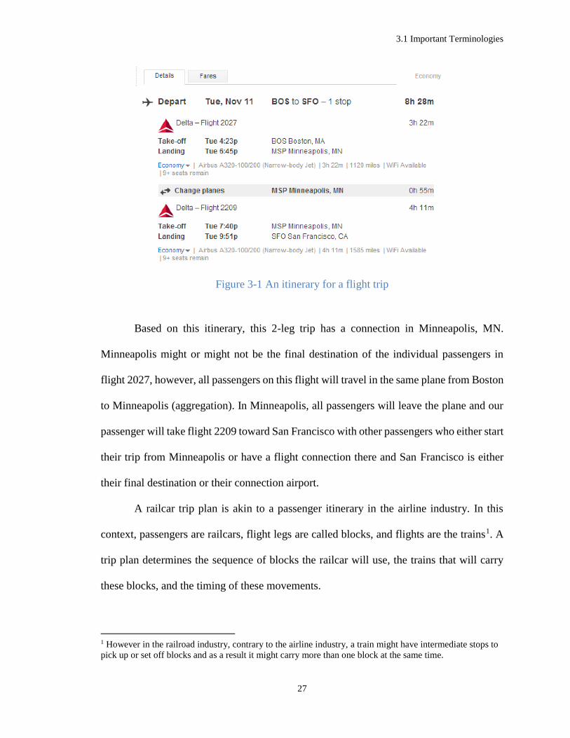
network in railroads is similar to the one in the airline industry. Figure 3-1 shows a
passenger itinerary for a customer who is planning to travel from Boston, MA to San
Francisco, CA on Tue, Nov 11.
3.1 Important Terminologies
27
Figure 3-1 An itinerary for a flight trip
Based on this itinerary, this 2-leg trip has a connection in Minneapolis, MN.
Minneapolis might or might not be the final destination of the individual passengers in
flight 2027, however, all passengers on this flight will travel in the same plane from Boston
to Minneapolis (aggregation). In Minneapolis, all passengers will leave the plane and our
passenger will take flight 2209 toward San Francisco with other passengers who either start
their trip from Minneapolis or have a flight connection there and San Francisco is either
their final destination or their connection airport.
A railcar trip plan is akin to a passenger itinerary in the airline industry. In this
context, passengers are railcars, flight legs are called blocks, and flights are the trains1. A
trip plan determines the sequence of blocks the railcar will use, the trains that will carry
these blocks, and the timing of these movements.
1 However in the railroad industry, contrary to the airline industry, a train might have intermediate stops to
pick up or set off blocks and as a result it might carry more than one block at the same time.

3.1 Important Terminologies
28
Similar to airline passengers, a set of cars can be grouped at a yard, then separated
into individual cars at a subsequent yard and again aggregated with different cars into a
different group. A set of railcars that are moved as a single group from one rail yard (block's
origin) to another (block's destination) is called a block and the process of aggregation and
separation of cars in the yards is referred to as Blocking or Classification. Block’s origin
and destination are predesigned in the tactical level. In fact block is a predesigned origin-
destination pair where all cars will be treated as a group as long as they are in the same
block. It is important to differentiate between blocks and shipments. 100 cars moving from
Boston to San Francisco are not necessarily considered a block the same way that a group
of 100 students flying from Boston to San Francisco doesn’t necessarily mean there is a
direct flight between these two cities. The individual cars within the block might have
different origins and destinations but will be treated as a unit in the part of the trip which
they share as a block.
Trip plans are generated based on the operating plan which consists of three main
components: a blocking plan, train routings, and a train makeup plan. Each of these
components by itself is an optimization problem that arises at tactical level. A blocking
plan can be derived from a block design problem that determines which blocks need to be
made at each rail yard, and what type of railcars are to be placed into each block. The train
routing problem is to identify the origin, destination, routes, frequencies, and timetables of
all trains to minimize the cost of carrying cars from their origins to their destinations. Once
the blocking plan and the train routings are ready, the next step is to determine which trains
should carry which blocks (train makeup or block to train assignment problem). Train
timetables and routes should be designed in such a way that they are consistent with the

3.2 Network Representation
29
rail network and the blocks to be transported. That is why the train routing and the train
makeup problem are often integrated into a single problem, called the train design problem.
Operating plan development is a tactical decision and is considered a service
network design problem (SNDP). In the operational level of decision making such as the
empty railcar allocations or car routing (trip planning) we realistically assume that the
operating plan is already developed and the operational decisions should be consistent with
this plan.
3.2 Network Representation
The network referred to in most part of this research, is the service network also
known as the railroad operating plan. The operating plan is designed on top of the physical
(geographical) railroad network where the track segment’s maximum tonnage enforces the
train capacities and the classification track lengths determine the block capacities. In this
section, we first present the static networks, i.e. without time dimension, including the
physical network and the static operating plan. This will give us the opportunity to explain
in detail the operating plan and the steps that are taken at the tactical level to design this
plan. Then, we add the time dimension to the network and create a time-space network
which is suitable for our dynamic car distribution model.
3.2.1 Static Networks
Figure 3-2(a) shows a geographical/physical railroad network of seven nodes and
nine arcs, where nodes correspond to the rail yards, and arcs correspond to the rail tracks,
also known as rail segments, connecting these yards. Designing/redesigning the
geographical railroad network is a strategic decision made by the highest management, and
in this research, we realistically assume that the physical network is given. Three trains 𝐴,

3.2 Network Representation
30
𝐵, and 𝐶 traveling in this network have been designed at the train routing level and are
shown in Figure 3-2(b). All trains start at node 1 and terminate at node 7, excepted train 𝐴
which terminates at node 6. Train 𝐴 uses path 1-2-6 while train 𝐵 and 𝐶 use path 1-4-5-6-
7 and 1-2-3-7 respectively. The blocking plan for this railroad consists of six blocks
𝑏1, … , 𝑏6. Figure 3-2(c) shows these blocks and regardless of the path, each block is
travelling in the railroad network. The block-to-train assignments are planned at the train
makeup level and the result is illustrated in Figure 3-2(d). Each block might use more than
one train segment or even more than one train from its origin to its destination; however,
it cannot be assigned to more than one train over one single railroad arc. For example block
𝑏1 takes only train 𝐴 over only one train segment 2-6, while block 𝑏6 takes the train 𝐵 over
the segments 5-6 and 6-7. Thus, as a train travels from its origin to its destination, it visits
various yards to pick up blocks (e.g. train 𝐶 at yard 1 picks up block 𝑏3), to drop off blocks
(e.g. train 𝐶 at yard 7 drops off block 𝑏5) or to perform both (e.g. train 𝐶 at yard 2 drops
off block 𝑏3 and picks up block 𝑏5). Typically, several blocks travel on a train at any
segment (e.g. blocks 𝑏1 and 𝑏4 travel on train 𝐴 on segment 2-6). On its way from the
origin to the destination, a block may also travel on several trains. Transferring a block
between trains without re‐classification of individual cars at yards is called a block swap.
For example, block 𝑏4 requires a block swap at yard 6 where it is set off by train 𝐴 and is
picked up by train 𝐵. During a block swap, the entire block of cars remains coupled
together while moving to another train, requiring less classification work comparing to the
reclassification of all individual cars in the block. In order to easily refer to different
segments of the trains moving on the network, in Figure 3-2(e) we have named each train
segment separately. For example arcs 𝐶1, 𝐶2 and 𝐶3 in this extended train network represent
3.2 Network Representation
31
train 𝐶 on segments 1-2, 2-3, and 3-7, respectively. From now on, unless specified
otherwise, with train we mean the train segment and with train network we mean the
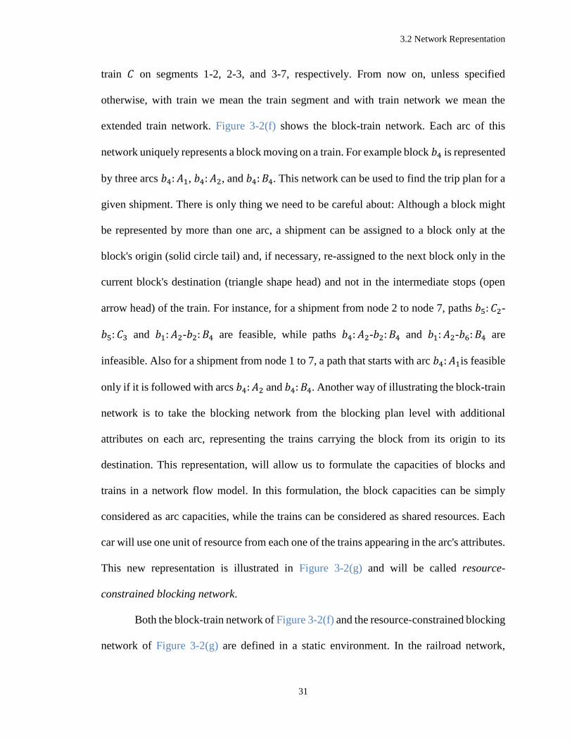
extended train network. Figure 3-2(f) shows the block-train network. Each arc of this
network uniquely represents a block moving on a train. For example block 𝑏4 is represented
by three arcs 𝑏4: 𝐴1, 𝑏4: 𝐴2, and 𝑏4: 𝐵4. This network can be used to find the trip plan for a
given shipment. There is only thing we need to be careful about: Although a block might
be represented by more than one arc, a shipment can be assigned to a block only at the
block's origin (solid circle tail) and, if necessary, re-assigned to the next block only in the
current block's destination (triangle shape head) and not in the intermediate stops (open
arrow head) of the train. For instance, for a shipment from node 2 to node 7, paths 𝑏5: 𝐶2-
𝑏5: 𝐶3 and 𝑏1: 𝐴2-𝑏2: 𝐵4 are feasible, while paths 𝑏4: 𝐴2-𝑏2: 𝐵4 and 𝑏1: 𝐴2-𝑏6: 𝐵4 are
infeasible. Also for a shipment from node 1 to 7, a path that starts with arc 𝑏4: 𝐴1is feasible
only if it is followed with arcs 𝑏4: 𝐴2 and 𝑏4: 𝐵4. Another way of illustrating the block-train
network is to take the blocking network from the blocking plan level with additional
attributes on each arc, representing the trains carrying the block from its origin to its
destination. This representation, will allow us to formulate the capacities of blocks and
trains in a network flow model. In this formulation, the block capacities can be simply
considered as arc capacities, while the trains can be considered as shared resources. Each
car will use one unit of resource from each one of the trains appearing in the arc's attributes.
This new representation is illustrated in Figure 3-2(g) and will be called resource-
constrained blocking network.
Both the block-train network of Figure 3-2(f) and the resource-constrained blocking
network of Figure 3-2(g) are defined in a static environment. In the railroad network,

3.2 Network Representation
32
blocks are statically defined as pairs of origin-destination and some other attributes such
as car type, freight type, etc. However, train schedules are dynamic. Some trains might run
every day or even more than once a day, while some others might run less than seven times
a week. A time-space network will add this dynamicity to the network representation.

3.2 Network Representation
33
Figure 3-2 Underlying networks used in the railroad optimization models

3.2 Network Representation
34
Figure 3-2 continued. Underlying networks used in the railroad optimization models
3.2 Network Representation
35
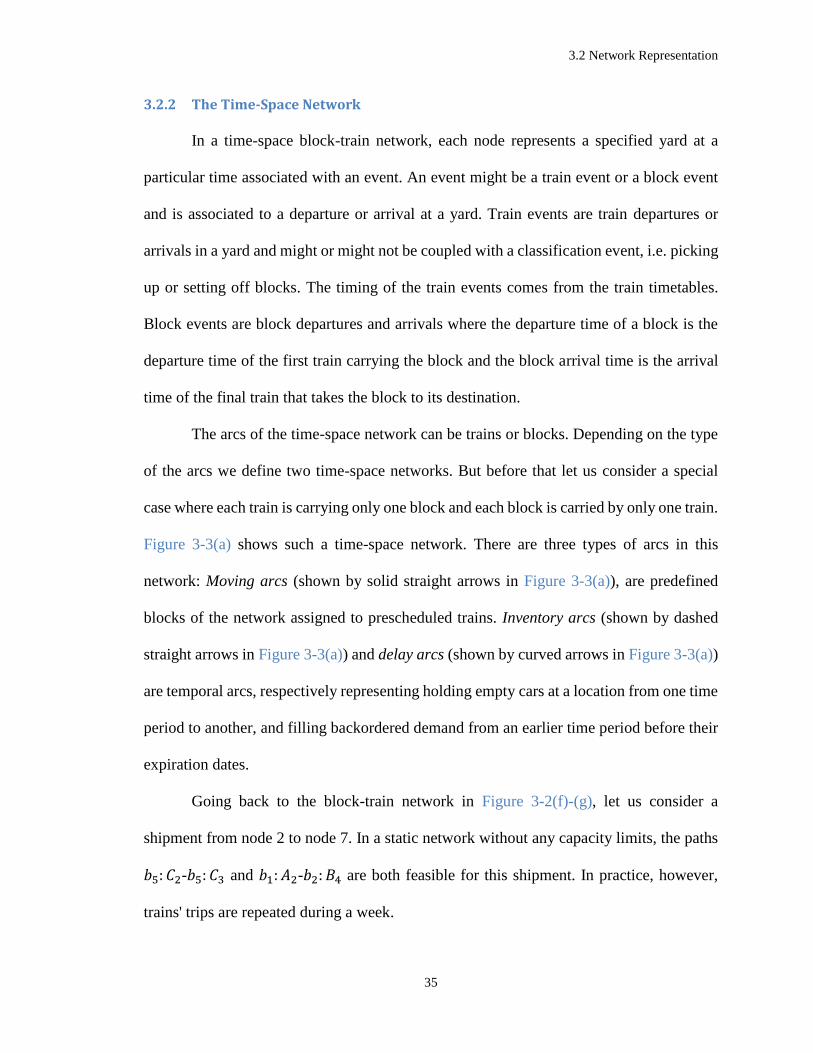
3.2.2 The Time-Space Network
In a time-space block-train network, each node represents a specified yard at a
particular time associated with an event. An event might be a train event or a block event
and is associated to a departure or arrival at a yard. Train events are train departures or
arrivals in a yard and might or might not be coupled with a classification event, i.e. picking
up or setting off blocks. The timing of the train events comes from the train timetables.
Block events are block departures and arrivals where the departure time of a block is the
departure time of the first train carrying the block and the block arrival time is the arrival
time of the final train that takes the block to its destination.
The arcs of the time-space network can be trains or blocks. Depending on the type
of the arcs we define two time-space networks. But before that let us consider a special
case where each train is carrying only one block and each block is carried by only one train.
Figure 3-3(a) shows such a time-space network. There are three types of arcs in this
network: Moving arcs (shown by solid straight arrows in Figure 3-3(a)), are predefined
blocks of the network assigned to prescheduled trains. Inventory arcs (shown by dashed
straight arrows in Figure 3-3(a)) and delay arcs (shown by curved arrows in Figure 3-3(a))
are temporal arcs, respectively representing holding empty cars at a location from one time
period to another, and filling backordered demand from an earlier time period before their
expiration dates.
Going back to the block-train network in Figure 3-2(f)-(g), let us consider a
shipment from node 2 to node 7. In a static network without any capacity limits, the paths
𝑏5: 𝐶2-𝑏5: 𝐶3 and 𝑏1: 𝐴2-𝑏2: 𝐵4 are both feasible for this shipment. In practice, however,
trains' trips are repeated during a week.

3.2 Network Representation
36
Figure 3-3 shows three paths, all associated to the static path 𝑏1: 𝐴2-𝑏2: 𝐵4, but this
time on a time-space network of blocks and trains. The sub indices T,W,R,F for train
(block) represent the day in which the train leaves the yard (block is created). For example,
arc 𝑏1𝑇: 𝐴2𝑇 refers to the block 𝑏1 which is created on Tuesday and is assigned to train 𝐴2
on Tuesday. The trip from 𝑠 to 𝑑 is not a direct trip and has a connection on the
classification yard 6. The green path starts from yard 2 on Tuesday when Train 𝐴2𝑇 pulls
block 𝑏1𝑇, which is carrying the car, to the block destination at yard 6. In the classification
yard 6, the car will be reclassified to the block 𝑏2𝑅 which is planned to be pulled by train
𝐵4𝑅 on Thursday. Finally, the car will arrive at the customer yard 7 (end of the physical
trip) on Sunday, which is one day later than the order date of customer 𝑑. This explains the
reason why a temporal delay arc connects this car to its corresponding demand day.
The blue path is generated by a similar trip plan, but the trip starts and ends one day
later. Another possible path from 𝑠 to 𝑑 is to start with train 𝐴2𝑇, wait one day in
classification yard 6, and finally take the train 𝐵4𝐹. Practically, if the number of cars
assigned to a block is more than the block size, the remaining cars will be classified in the
next day. While the mileage cost of both Green and Blue paths are similar, the total cost
associated to the blue path is likely to be higher as a result of the inventory costs at the
beginning of the trip, and an extra day of delay at the destination.
3.2 Network Representation
37
a)
Yar
d
2 7 6 M T W R F S N M
Time
b)
Figure 3-3 The time-space network (a) and its associated multigraph (b)
3.2.2.1 The Time-Space Block-Train Network
The time-space network of Figure 3-3(a) is not realistic since in practice trains
might carry multiple blocks at a time and a block might be carried on multiple trains (train
segments) throughout its destination. Therefore a single arc cannot represent a single train
and a single block at the same time. The time-space network presented in this section is a
block-train network, where events are train events. This network is a multigraph and there
exist one arc for each train and each block carried on that train.
Figure 3-4 shows the entire time-space block-train network associated with the
static block-train network of Figure 3-2(f) in a 6-day time horizon. Similar to the static
block-train network arrows have two different types of tail and heads, where only a solid
circle represents a block origin and a triangle shape head represents a block destination.
Unlike Figure 3-3(a), in this figure we do not show the delay arcs, since delays are
associated to the shipments and not to the operating plan of the railroad.
𝑑
𝑠
2
6
7
𝑏1𝑊: 𝐴2𝑊 𝑏1𝑇: 𝐴2𝑇 𝑏2𝑅: 𝐵4𝑅
𝑏2𝐹: 𝐵4𝐹
𝑏1𝑇: 𝐴2𝑇
𝑏1𝑊: 𝐴2𝑊 𝑏2𝐹: 𝐵4𝐹
𝑏2𝑅: 𝐵4𝑅

3.2 Network Representation
38
Figure 3-4 Time-space block-train network associated to Figure 3-2(f)

3.2 Network Representation
39
3.2.2.2 The Time-Space Resource Constrained Blocking Network
The time space network presented in train-block network is defined on top of the
train networks. In US railways, shipments are assigned to blocks and blocks are carried by
trains. This is why a service network defined on top of the blocking network, rather than
the train network, is more applicable to the US railways. Figure 3-5 shows the resource
constrained blocking network associated to the time space block-train network of Figure
3-4. Nodes in this network are associated to block events in classification yards, where a
block event means a block departure or arrival at a classification or serving yard. Timing
of block events is known beforehand from block to train assignment plan in tactical level.
Arcs are the blocks and the inventory arcs connecting the nodes associated to the same yard
and trains carrying those blocks are listed as the resources used by the blocks. Figure 3-6
is basically the same as Figure 3-5; with less visualization on the train changes. In this
research, unless specified otherwise, whenever talking about time-space network, we refer
to Figure 3-6. Customers are located in the nodes of the time-space network. Figure 3-7
shows three customer profiles on the time-space blocking network, two of them, C1 and
C2, are located in yard 2 and the third one is located in yard 7. Demand nodes are shown
by rectangular and those associated with the same customer profile in different days are
connected using delay arcs. It is noteworthy that this network can be considered as a two-
layer network: a) the time-space network layer which is constructed by inventory arcs and
moving arcs (blocks) and b) the customer layer which is constructed by the delay arcs. The
two layers are connected using intraarcs that transfer the flow of cars from the time-space
network to the customers.
It is worth mentioning that the car routing (trip planning) between supply and
demand nodes is not an output of the distribution model, but an input to it. The selection
3.2 Network Representation
40
of either the green or the blue path in Figure 3-3 will result in the same assignment of s to
d, from the same physical route but in different days. In other words, the output of the
assignment model is the decision about when and where to send the car, while the
corresponding route for the trip is decided by the trip plan application.

3.2 Network Representation
41
Figure 3-5 Time-space resource-constrained block network (colors for visualization)

3.2 Network Representation
42
Figure 3-6 Time-space resource-constrained block network (the main representation)

3.2 Network Representation
43
Figure 3-7 Customers on time-space resource-constrained block network

3.2 Network Representation
44
3.2.3 The Bipartite Multigraph
Similar to the transportation problem formulation, network used for car distribution
in noncapacitated networks is a bipartite supply-demand graph. Similar graph can be used
for the path-based formulation of the capacitated model. However if more than one path
exists between some supply-demand pairs, the network will be a bipartite multigraph.
Nodes of this graph as is shown in Figure 3-8 are from two layers of supply nodes and
demand nodes. In this graph there is one supply node for each yard, for each time period
and for each pool available at that yard and there is one demand node for each customer
profile, for each day. One super supply node and one super demand node will be added to
maintain the supply-demand balance. Eligible and feasible supply and demand nodes are
connected using at least one arc where, as will be discussed in Section 3.5, eligibility is
defined based on attribute matching between supply-order pair and feasibility is defined
based on order fulfilment before its expiration date.
Figure 3-8 Bipartite supply-demand multigraph

3.2 Network Representation
45
3.2.4 Network Capacities
Cars are carried on blocks, and blocks are pulled by trains. Both blocks and trains
have capacity limits. Blocks are created on the classification yards. Normally each block
is created on one rail track in the classification yard. Tracks in classification yards have
fixed length and as a result each block also has a length. Furthermore, the number of blocks
created in a classification yard sometimes exceeds the number of classification tracks in
the yard; hence reducing the number of blocks to be built, by charging a setup cost on
blocks, might improve the yard operations. However, before running the empty car
distribution model, many of these blocks are already planned as a result of currently
planned loaded or empty car movements. This is the reason that the setup cost should be
charged only on the blocks that will be created in bottleneck yards and only when they are
created as a result of empty car distribution model.
Trains travel over the physical railroad network. Depending on the geography of
the area and the rail track attributes, certain segments of the network might have limitations
on the maximum train length and weight. Assuming that train length constraints have been
already satisfied at the tactical level of the block to train assignment decision making
process, the train weight limits still need to be considered in the operational models such
as trip planning and car distributions.
3.2.5 Cost Components
While the complexity of linear programs mainly depends on the number and type
of constraints and decision variables, the usefulness of the optimal solution also depends
on the cost coefficients. This means that formulating the problem as a complex
mathematical model that considers all business rules and limitations is not sufficient for

3.2 Network Representation
46
having a desirable output unless the coefficients of the objective function are realistically
chosen and calibrated. In this research, instead of randomly generating the cost coefficients,
we develop a systematic approach on calculating the cost coefficients.
Figure 3-9 shows part of the time-space network. Let’s consider a shipment of a
railcar of pool k from supply node m to the demand node n on the bold dark blue path. The
costs associated with this shipment are 𝑐𝑖𝑘 on inventory arc 𝑖, 𝑐𝑏
𝑘 on block 𝑏, 𝑐𝑛+1𝑘 the
fulfillment cost/credit, and 𝑐𝑑𝑑𝑒𝑙𝑎𝑦
the delay cost. In mathematical language if we note this
path by 𝑙 the total cost associated to it is calculated as 𝑐𝑙𝑘 = 𝑐𝑖
𝑘 + 𝑐𝑏𝑘 + 𝑐𝑛+1
𝑘 + 𝑐𝑑𝑑𝑒𝑙𝑎𝑦
.
Now we explain each term in this function. 𝑐𝑖𝑘 is the unit inventory cost and as
stated in (3-1) depends on the number of days in the inventory arc and the car hire rate per
day. Car hire is the rate that the railroad is paying for leasing a car or the rate that a railroad
can lease out its car to other railroad if not used in its own network. The “$” sign in cost
parameter definitions (3-1) to (3-7) represents a constant rate and the suggested rates are
given in Table 3-1. 𝑐𝑏𝑘 is the variable cost of block b and as in (3-2) has three components:
a constant part as classification cost for each car at the block origin classification yard and
two other parts that depend on how many days and miles it takes from block’s origin to its
destination. 𝑐𝑛𝑘 is the cost/credit of fulfilling one unit of demand of customer 𝑛 by a car of
pool 𝑘 and based on (3-3) depends on how good fit the car is to the order and how important
the customer, more specifically the demand node, is to the railroad. The best way to
measure the customer importance is to see how much profit will be collected by fulfilling
the customer’s demand. However in the railroad industry, the loaded destination of an
empty car requested by a customer is not known unless it is loaded, which clearly is not
the case in the car distribution planning time. However, by analyzing the historical data,
3.2 Network Representation
47
railroad carrier can prioritize some customers and give a virtual credit for fulfilling demand
of high priority customers. It is also important to be clear about what a higher priority
customer implies: An absolute customer priority over another customer means that if two
customers are at the same location, the high priority customer’s demand, no matter for what
day, is of more importance than the other customer’s. A proportional priority applies the
priorities only for the same days. A middle approach is presented in Table 3-2 where if
three customers 1, 2, and 3 of priority 1, 2, and 3 are located in the same yard, the demand
of customer 3 in days 1 and 2 has higher priority over customer’s 2 demand for day 1.
However this customer’s demand for day 3 will be satisfied after customer 2 demand for
day 1 is satisfied. Finally 𝑐𝑑𝑑𝑒𝑙𝑎𝑦
in (3-4) is the adjusted delay cost and depends on how late
the shipment will arrive to the customer. As mentioned before the fulfillment cost/credit
considered in 𝑐𝑙𝑘 is 𝑐𝑛+1
𝑘 and not 𝑐𝑛𝑘. This is why the delay cost 𝑐𝑑
𝑑𝑒𝑙𝑎𝑦 is adjusted by 𝑐𝑛
𝑘 −
𝑐𝑛+1𝑘 to reflect the correct cost coefficients.
The above mentioned cost components are associated with the variable costs of
assignment. Two other cost components are the fixed cost associated with block setups
(3-5) and the shortage penalties.
In real world applications the supply and demand are not necessarily balanced. In
fact in our application, since supply is usually on hand while demand is for a two week
time horizon, supply is always less than demand. Hence shortage is inevitable. Each unit
of unmet demand is penalized by 𝑐𝑛. Designing the shortage penalty is extremely
important. Assigning a very large number, a Big M, to 𝑐𝑛 will transform the problem from
an assignment cost minimization problem to an order fulfilment maximization problem
regardless of customer priorities and their pool preferences. This is why a trade-off between

3.2 Network Representation
48
assignment costs and shortage penalties must be considered while assigning the shortage
penalties. The shortage penalty 𝑐𝑛 depends on how much money the railroad is willing to
spend on pulling an empty railcar in general to satisfy an order and specifically this order.
Equation (3-7) shows how to calculate a minimum penalty cost based on how many miles
and days and classifications, in general, a railroad is willing to spend to fulfill a general
customer demand. This value is used in (3-6) to calculate the unmet demand penalty for a
specific demand node where a demand node with higher priority is penalized more
compared to the ones with lower priorities.
𝑐𝑖𝑘 = numWaitingDays * $carHirePerDay (3-1)
𝑐𝑏𝑘 = numTravelDays * $carHirePerDay + numTravelMiles *
$carHirePerMile + 1 * $classificationPrice
(3-2)
𝑐𝑛𝑘 = (pref (k) - 1) * $prefValue - priority (n) * $priorityValue (3-3)
𝑐𝑑𝑑𝑒𝑙𝑎𝑦
= delay * $latePenalty + 𝑐𝑛𝑑𝑘 − 𝑐𝑛𝑜
𝑘 , where 𝑛𝑜 and 𝑛𝑑 are the origin
and destination of delay arc 𝑑.
(3-4)
𝑓𝑏 = $blockSetupCost(b) (3-5)
𝑐𝑛 = [minPenCost + acceptedDelay (n) * $latePenalty +
(worseAcceptedPoolPref (n) - 1) * $prefValue] * (1 + priority (n))
(3-6)
minPenCost = maxAcceptedMile4EmptyTrip * $carHirePerMile +
maxAcceptedDays4EmptyTrip * $carHirePerDay +
maxAcptdNumOfClassfication4EmptyTrip * $classificationPrice
(3-7)

3.2 Network Representation
49
Table 3-1 Parameters used to calculate the cost coefficients
Parameter Suggested Value
$carHirePerDay 24
$carHirePerMile 0.83
$classificationPrice 50
$latePenalty 100
$prefValue 50
$priorityValue 100
acceptedDelay(n) 0,1,2,3,4
maxAcceptedMile4EmptyTrip 400
maxAcceptedDays4EmptyTrip 6
maxAcptdNumOfClassfication4EmptyTrip 4
pref (k) 1,2,3 where 1 is the best match
priority(n) [0-3] where 3 has highest priority
𝑓𝑏 = (uni (0, 1) < ratioOfBlocksWithSetupCost) *
c_maxBlockFixedCost * uni (0, 1)
c_maxBlockFixedCost 3000
ratioOfBlocksWithSetupCost 0.1
Table 3-2 Demand node priorities based on customer priorities
Figure 3-9 Costs on the time space network
1 2 3 4 5 6 7 8 9 10 11 12 13 14
1 1 0.707 0.5 0.354 0.25 0.177 0.125 0.088 0.063 0.044 0.031 0.022 0.016 0.011
2 2 1.414 1 0.707 0.5 0.354 0.25 0.177 0.125 0.088 0.063 0.044 0.031 0.022
3 3 2.121 1.5 1.061 0.75 0.53 0.375 0.265 0.188 0.133 0.094 0.066 0.047 0.033Cu
sto
me
Pri
ori
ty
Day
𝑛 + 1
𝑚, 𝑠𝑚𝑘
𝑐𝑑𝑑𝑒𝑙𝑎𝑦
𝑐𝑖𝑘
𝑓𝑏 , 𝑐𝑏𝑘
𝑐𝑛+1𝑘
𝑚′ + 1 𝑚′ 𝑚′ − 1
𝑚 + 1
𝑛, 𝑑𝑛, 𝑐𝑛 𝑛 + 2
𝑐𝑛𝑘

3.3 Fleet
50
3.3 Fleet
Freight cars are categorized in different car types mainly based on the nature of
goods which are going to be shipped by the car. For example, box cars are fully enclosed
cars with side or end doors and are good for transporting moisture-susceptible goods; coil
cars are good for carrying heavy sheet metal rolls; and flatcars are mainly used for shipping
automobiles. Generally speaking, substitution across car types is typically not possible and
traditionally, different car types are managed separately. However, all the cars of the same
type are not exactly the same. For example, boxcars might have one door or two.
Furthermore, the doors might be plug doors which open with a hand crank, or sliding doors,
which may require opening with a forklift. Some customers might have a preference
between cars from the same type. This is one of the reasons why railroads further classify
cars within a car type into smaller groups named pools. From order fulfillment perspective,
cars within a pool can be considered exactly the same. The number of pools in a single car
type typically ranges between 5 and 20. As a general rule, a customer will require a number
of cars from a particular set of pools along with their preferences or will specify a car type
as well as some extra requirements which can be translated into priorities among pools
within that car type. Substitutability is an attribute of demand and not car type; in other
words substitutability is demand specific. This means that pool 1, in car type 1, might be
substitutable by pool 2, also in car type 1, for customer A, while customer B only accepts
pool 1.
3.4 Customer, Customer profile, Demand node and Demand
A customer is a client located on the railroad network who orders empty railcar
from railroad. Each customer might have one or more profiles. A profile consists of a set

3.4 Customer, Customer profile, Demand node and Demand
51
of pools and the preferences among them. Preferences are integer values of 1, 2, or 3 and
will be used while calculating the assignment costs. While the optimization model will try
to fulfill the customers demand from higher preference pools, in the presence of supply
limitation it is not guaranteed. In fact any assignment from the set of pools listed in the
customer’s profile is acceptable to the customer, even if they all come from the customer’s
lowest preference. Any criteria on the minimum or maximum number of cars from one
specific pool among the accepted pools (as in case 3 in Table 3-3) should be handled
explicitly, for example by introducing a new customer profile (case 3-1 and 3-2).
A demand node represents a customer profile on a specific day. For example, in a
two-week ahead planning strategy, each customer profile will be associated with a
maximum of 14 demand nodes and less than that if they do not order all days. Demand in
this research means the number of cars that a customer has ordered from a specific profile
and for a specific day, and basically is associated to a demand node. Furthermore, if part
of customer’s demand is already fulfilled, the demand should be modified by excluding the
fulfilled part. In this research unless specified otherwise, the demand refers to the modified
demand and not to the original customer’s demand.
Table 3-3 Illustration of customer profiles
Case
Customer
Location (serving yard)
Customer Profile
Accepted pools
Preferences
Two-week Demand
Extra condition
OK?
1 X 123 X1 {1,2,3} {1,1,2} 100 NA OK 2 X 123 X2 {4,5} {1,1} 50 NA OK 3 Y 451 Y1 {1,2,3} {1,2,2} 50 At least
10 from pool 1
NO
3-1 Y 451 Y1-1 {1} {1} 10 OK 3-2 Y 451 Y1-2 {1,2,3} {1,2,2} 40 OK

3.5 Supply
52
3.5 Supply
Supply is the fleet that is available for assignment and is a subset of fleet that can
be assigned to the customer orders. For a railcar to be considered as supply it should be
suitable, serviceable, distributable, and optimizeable and to be considered eligible for a
given customer profile it should match the order’s attributes (pool matching) and to be
considered feasible for a given demand node (i.e. in a specific day) it should arrive before
the order expiration date. Below we explain all these keywords.
Suitable: a car is considered suitable for the customer orders if its pool number matches at
least one of the customer profiles in the planning horizon. If a car is not suitable it means
it is out of the scope of the supply-order matching.
Serviceable: a railcar is serviceable if it is not in bad order or rejection status. A serviceable
car is either currently serving a customer or on the way to a customer or available to serve
a customer.
Distributable: a railcar is distributable if the car distribution department has the authority
to distribute this car. For example, foreign cars that belong to other railway carriers, private
cars that are property of a customer and only hauled by the railway, and dedicated pool
cars that are usually assigned to major customers, unless there is an agreement, are not
distributable.
Optimizeable: a railcar is considered optimizeable in operating station A and time T if it
is guaranteed that it will be empty in that time and location, is not assigned to a customer
or can be reassigned if it is already assigned to one. As a special case a suitable, serviceable
and distributable car that is already empty (time zero) at station A and is not assigned to
any customer is optimizeable now at station A and can be considered as supply.

3.5 Supply
53
Eligible: a car is eligible to be assigned to a customer profile if its pool number matches
that profile.
Feasible: assignment of a car to a demand node is considered feasible if it is eligible and
can arrive to customer facility before the order expiration date.
Optimization model will be run on the feasible assignments to find the optimal
assignments. The output of the model after CDU confirmation/modification is considered
Planned and once is billed to a customer is considered Assigned.
Note: a situation of having cars not planned is most likely to happen when we are
in a global or local surplus situation. A local surplus situation means we have excess of
cars in an area that their assignment to the current demand is either not feasible or not
economic. In order to avoid sleep of fleet, railroad should consider some storage facilities
in different parts of the railroad network, as low priority customers; otherwise, the
optimizer will leave them as not planned cars or leftover supply.
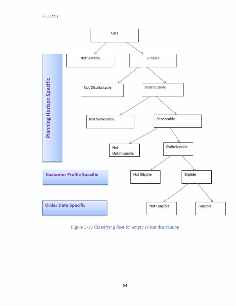
3.5 Supply
54
Figure 3-10 Classifying fleet for empty railcar distribution
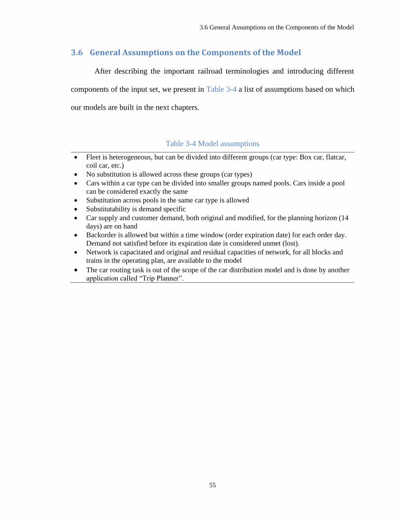
3.6 General Assumptions on the Components of the Model
55
3.6 General Assumptions on the Components of the Model
After describing the important railroad terminologies and introducing different
components of the input set, we present in Table 3-4 a list of assumptions based on which
our models are built in the next chapters.
Table 3-4 Model assumptions
Fleet is heterogeneous, but can be divided into different groups (car type: Box car, flatcar,
coil car, etc.)
No substitution is allowed across these groups (car types)
Cars within a car type can be divided into smaller groups named pools. Cars inside a pool
can be considered exactly the same
Substitution across pools in the same car type is allowed
Substitutability is demand specific
Car supply and customer demand, both original and modified, for the planning horizon (14
days) are on hand
Backorder is allowed but within a time window (order expiration date) for each order day.
Demand not satisfied before its expiration date is considered unmet (lost).
Network is capacitated and original and residual capacities of network, for all blocks and
trains in the operating plan, are available to the model
The car routing task is out of the scope of the car distribution model and is done by another
application called “Trip Planner”.

4.1 A General Integer Programming Formulation
56
Chapter 4
4 Path-Based Formulation for Car
Distribution Problem
4.1 A General Integer Programming Formulation
Let 𝛹 represent the set of all pools of cars that appear in customers’ demand. Set
𝛹 can be partitioned into a collection of some number of nonempty subsets of pools that
are mutually exclusive and collectively exhaustive, representing different car types. Supply
is a tuple (𝐾 ⊆ 𝛹, 𝑘 ∈ 𝐾 ,𝑚 ∈ 𝑀, 𝑠𝑚𝑘 ) where 𝐾 ⊆ 𝛹, 𝑘 ∈ 𝐾 represents a car type and car
pool, respectively; 𝑚 ∈ 𝑀 is a node in the time-space network, and 𝑠𝑚𝑘 is the number of
cars of pool 𝑘 available at node 𝑚. Demand is also a tuple (𝐾 ⊆ 𝛹, 𝑛 ∈ 𝑁𝐾, 𝑝𝑟𝑖(𝑛), 𝐾𝑛 ⊆
𝐾, 𝑝𝑟𝑒𝑓(𝑘), 𝑑𝑛, 𝑦𝑛𝑚𝑎𝑥, 𝑒𝑥𝑝(𝑛)) where 𝐾 ⊆ 𝛹 is the car type that the demand belongs to;
𝑛 ∈ 𝑁𝐾 represents the customer index in the time space network; 𝑝𝑟𝑖(𝑛) → 𝑅+ is function
that returns the importance to fulfill this demand compared to other demands; 𝐾𝑛 ⊆ 𝐾 is
the set of pools which are eligible to fulfill customer needs, and 𝑝𝑟𝑒𝑓(𝐾𝑛) → 𝑅|𝐾𝑛|+ is a
function representing the preference of customer/railroad within these eligible pools; 𝑑𝑛 is
the modified demand of the customer and is calculated from subtracting part of the demand
that has been already fulfilled, 𝑎𝑛, from the original demand, 𝑑′𝑛; and 𝑒𝑥𝑝(𝑛) is order

4.1 A General Integer Programming Formulation
57
expiration date after which date the demand is lost; meaning that if the car arrives after that
date, the customer will not be able to use it against this demand.
Table 4-1 contains the indices, sets, parameters and decision variables that are used
in the mathematical model. Some elements of the demand tuple such as
𝑝𝑟𝑖(𝑛), 𝑝𝑟𝑒𝑓(𝐾𝑛), 𝑒𝑥𝑝(𝑛) are not listed in this table. This is not because these elements
(parameters) are not important, but because they do not appear in the mathematical model
directly. However, we use these parameters to calculate the cost coefficients associated
with the objective function. Please see Section 3.2.5 for details on how to calculate the cost
parameters. After introducing the model parameters, we start formulating the car
distribution optimization model.
The objective function (4-1) minimizes the total cost of empty car repositioning
plan which includes the setup cost of new blocks, the transportation costs, and the unmet
demand penalties. Since in the scheduled railroads, general trains are unlikely to be
canceled at the operational planning level, train setup cost is not considered in this model.
𝑀𝑖𝑛 ∑𝑓𝑏𝑧𝑏𝑏∈𝐵
+ ∑ ∑ 𝑐𝑙𝑘 𝑥𝑙
𝑘
𝑘∈𝐾,𝐾⊆𝛹𝑙∈𝐿
+ ∑ 𝑐𝑛 𝑦𝑛𝑛∈𝑁𝐾,𝐾⊆𝛹
(4-1)
Constraint (4-2) assures that the number of cars of each pool moved from node m
does not exceed its available supply. Constraint (4-3) defines variable 𝑦𝑛 (unmet demand)
as the demand of customer at node n minus the number of cars that customer receives.

4.1 A General Integer Programming Formulation
58
Table 4-1 Mathematical notation
Indices and Sets
𝑘 ∈ 𝐾 Index for pools that belong to a specific car type
𝑚 ∈ 𝑀 Index for supply nodes in a time-space network
𝑛 ∈ 𝑁𝐾 Index for demand nodes in a time-space network
𝑏 ∈ 𝐵 Index for blocks
𝑔 ∈ 𝐺 Index for trains
𝑝 = {(𝑏1, 𝑔1), (𝑏2, 𝑔2), . . }∈ 𝑃
Index for trip plans. Each trip plan is an ordered set of blocks
carrying the cars and the trains carrying the blocks, 𝑏1, 𝑏2, … ∈𝐵 and 𝑔1, 𝑔2, … ∈ 𝐺 .
𝑙 = (𝑚, 𝑛, 𝑝) ∈ 𝐿 Index for supply-demand paths, or simply saying paths, in a
time-space network. A path 𝑙 = (𝑚, 𝑛, 𝑝) connects supply node
𝑚 and demand node 𝑛 through trip plan 𝑝.
𝐿𝑚𝑜 ⊆ 𝐿 Set of all paths that originate from node 𝑚
𝐿𝑛𝑑 ⊆ 𝐿 Set of all paths that end at node 𝑛
𝐿𝑏 ⊆ 𝐿 Set of all paths that use block 𝑏
𝐿𝑔 ⊆ 𝐿 Set of all paths that use train 𝑔
𝐾 ⊆ 𝛹 Set of pools representing a specific car type
𝐾𝑛 ⊆ 𝐾 Set of all pools eligible for demand node 𝑛
Parameters
𝑓𝑏 Setup cost for block 𝑏
𝑐𝑙𝑘 Unit cost for sending a car of pool 𝑘 on path 𝑙
𝑐𝑛 Unit cost of unmet demand (penalty) for demand node 𝑛
𝑐′𝑛 Unit cost of unmet demand (penalty) beyond for demand node 𝑛
𝑢𝑔 Capacity of train 𝑔 (train tonnage)
𝑣𝑏 Capacity of block 𝑏 (block length)
𝜇𝑙𝑘 Substitution ratio of a car of pool 𝑘 in path 𝑙. For example,
𝜇𝑙𝑘 = 2 means that a car from pool 𝑘 originating from node 𝑚,
where 𝑙 ∈ 𝐿𝑚𝑜 , having destination at demand node 𝑛, where 𝑙 ∈
𝐿𝑛𝑑 , will fulfill 2 units of demand of node 𝑛.
𝜔𝑘 Weight of an empty car of pool 𝑘
𝜏𝑘 Length of an empty car of pool 𝑘
𝑠𝑚𝑘 Supply of cars of pool 𝑘 in supply node 𝑚
𝑑𝑛 Demand of cars at demand node 𝑛 calculated as original
demand, 𝑑′𝑛 , minus fulfilled demand so far, 𝑎𝑛.
𝑦𝑛𝑚𝑎𝑥 Soft bound on the maximum unmet demand of demand node 𝑛
(Service level of demand node 𝑛).
Decision variables
𝑥𝑙𝑘 number of cars of pool 𝑘 to be sent on path 𝑙 to fulfill the order
of the associated customer
𝑧𝑏 Binary variable, 1 if block 𝑏 is created, and 0 otherwise
𝑦𝑛 Unmet demand of demand node 𝑛
𝑦′𝑛 Unmet demand of demand node 𝑛, beyond its soft bound, 𝑦𝑛𝑚𝑎𝑥

4.1 A General Integer Programming Formulation
59
∑ 𝑥𝑙𝑘 ≤ 𝑠𝑚
𝑘
𝑙∈𝐿𝑚𝑜
∀ 𝑚 ∈ 𝑀, ∀𝑘 ∈ 𝐾
∑ ∑ 𝜇𝑙𝑘𝑥𝑙
𝑘
𝑘∈𝐾𝑛𝑙∈𝐿𝑛𝑑
+ 𝑦𝑛 = 𝑑𝑛 ∀ 𝑛 ∈ 𝑁𝐾}
∀ 𝐾 ⊆ 𝛹
(4-2)
(4-3)
Constraints (4-4) and (4-5) apply capacity limits on the trains and blocks,
respectively.
∑ ∑ 𝜔𝑘𝑥𝑙𝑘
𝑘∈𝐾,𝐾⊆𝛹𝑙∈𝐿𝑔
≤ 𝑢𝑔 ∀𝑔 ∈ 𝐺 (4-4)
∑ ∑ 𝜏𝑘𝑥𝑙𝑘
𝑘∈𝐾,𝐾⊆𝛹𝑙∈𝐿𝑏
≤ 𝑣𝑏𝑧𝑏 ∀ 𝑏 ∈ 𝐵 (4-5)
Finally customer service levels are formulated as bounds on the unmet demand in
constraint set (4-6), assuring that unmet demand of each demand node is less than a
premised value.
𝑦𝑛 ≤ 𝑦𝑛𝑚𝑎𝑥 ∀ 𝑛 ∈ 𝑁𝐾, ∀ 𝐾 ⊆ 𝛹 (4-6)
Furthermore, all variables are nonnegative, flow variables 𝑥𝑙𝑘 are general integers
and block creation variables 𝑧𝑏 are binary. The shortage variables 𝑦𝑛 are not necessarily
integer if fractional numbers are permitted for 𝜇𝑙𝑘, and their integrality is guaranteed if
otherwise.
Assigning a bound on customer’s maximum accepted unmet demand in (4-6) is an
effort to increase the equity and fairness among the customers while optimizing the
efficiency of the system as a whole. Such bound might be enforced by the customer or
might be assigned by the car distribution department of the railroad. However it is
4.1 A General Integer Programming Formulation
60
important to keep in mind that by the time we are running the model some cars might have
been already assigned to the customer. Such a situation is likely to happen when the model
is run frequently, for example every one or two hours, if new supply of cars is detected or
for re-optimizing the previously made decisions. Simply saying, the demand 𝑑𝑛 in this
formulation might not necessarily be equal to what customer has asked in the first place
(i.e. the original demand) but part of the demand that is not yet satisfied before this run
(i.e. the modified demand). Equation (4-7) shows how the modified demand of demand
node 𝑛, 𝑑𝑛, is calculated based on its original demand, 𝑑′𝑛, minus the part of demand that
is fulfilled/planned so far, 𝑎𝑛.
𝑑𝑛 = 𝑑′𝑛 − 𝑎𝑛 ∀ 𝑛 ∈ 𝑁𝐾, ∀ 𝐾 ⊆ 𝛹 (4-7)
However with regard to the fairness among customers, the service level should be
applied against the original demand and not the modified demand. Hence, if the service
level of node 𝑛, is noted by 0 ≤ 𝜌𝑛 ≤ 1, then the maximum acceptable unmet demand can
be calculated as:
𝑦𝑛𝑚𝑎𝑥 = (1 − 𝜌𝑛) 𝑑
′𝑛 ∀ 𝑛 ∈ 𝑁𝐾, ∀ 𝐾 ⊆ 𝛹 (4-8)
During the validation process using randomly generated problems, we noticed that
in many cases the problem becomes infeasible. From a theoretical perspective, infeasibility
can happen in many mathematical programs, but when it goes to real world applications,
such a situation is not acceptable. After investigating the issue, the hard upper bounds on

4.1 A General Integer Programming Formulation
61
unmet demand in constraint (4-8) were detected as the source of the infeasibility. In order
to overcome this problem, the unmet demand above the upper bound was permitted but
with a higher penalty cost. This change was performed by replacing the hard constraints in
(4-8) by softer constraints as:
𝑦′𝑛 ≥ 𝑦𝑛 − 𝑦𝑛𝑚𝑎𝑥 ∀ 𝑛 ∈ 𝑁𝐾, ∀ 𝐾 ⊆ 𝛹 (4-9)
and adding another term, ∑ 𝑐′𝑛 𝑦′𝑛𝑛∈𝑁𝐾,𝐾⊆𝛹 , to the objective function. The new objective
function will be:
𝑀𝑖𝑛 ∑𝑓𝑏𝑧𝑏𝑏∈𝐵
+ ∑ ∑ 𝑐𝑙𝑘 𝑥𝑙
𝑘
𝑘∈𝐾,𝐾⊆𝛹𝑙∈𝐿
+ ∑ 𝑐𝑛 𝑦𝑛𝑛∈𝑁𝐾,𝐾⊆𝛹
+ ∑ 𝑐′𝑛 𝑦′𝑛𝑛∈𝑁𝐾,𝐾⊆𝛹
(4-10)
Constraint (4-9), will resolve the potential infeasibility caused by the enforced
service levels. The use of sign “≥” in this constraint, instead of a “=” sign, prevents the
model from another infeasibility situation in case 𝑦𝑛 < 𝑦𝑛𝑚𝑎𝑥. It should be noted that the
corresponding term in the minimizing objective function (4-10), ∑ 𝑐′𝑛 𝑦′𝑛𝑛∈𝑁𝐾,𝐾⊆𝛹 , will
guarantee that in the optimal solution constraint (4-9) is satisfied as an equality (
𝑦′𝑛 = 𝑦𝑛 − 𝑦𝑛𝑚𝑎𝑥) whenever 𝑦𝑛 ≥ 𝑦𝑛
𝑚𝑎𝑥 and 𝑦′𝑛 = 0 whenever 𝑦𝑛 < 𝑦𝑛𝑚𝑎𝑥. The effective
unmet demand cost then can be formulated as a piecewise linear function as in (4-11) and
is illustrated in Figure 4-1.

4.1 A General Integer Programming Formulation
62
𝑢𝑛𝑖𝑡𝑈𝑛𝑚𝑒𝑡𝐶𝑜𝑠𝑡 = {𝑐𝑛, ∀ 𝑦𝑛 ≤ 𝑦𝑛
𝑚𝑎𝑥
𝑐𝑛 + 𝑐′𝑛, ∀ 𝑦𝑛 > 𝑦𝑛
𝑚𝑎𝑥 (4-11)
Figure 4-1 Shortage cost function
The path-based formulation of the car distribution problem is presented as follows:
PathBased:
𝑀𝑖𝑛 ∑ 𝑓𝑏𝑧𝑏𝑏∈𝐵 + ∑ ∑ 𝑐𝑙𝑘 𝑥𝑙
𝑘𝑘∈𝐾,𝐾⊆𝛹𝑙∈𝐿 + ∑ 𝑐𝑛 𝑦𝑛𝑛∈𝑁𝐾,𝐾⊆𝛹 +
∑ 𝑐′𝑛 𝑦′𝑛𝑛∈𝑁𝐾,𝐾⊆𝛹
(4-12)
∑ 𝑥𝑙𝑘 ≤ 𝑠𝑚
𝑘𝑙∈𝐿𝑚
𝑜 ∀ 𝑚 ∈ 𝑀,∀𝑘 ∈ 𝐾 ⊆ 𝛹 (4-13)
∑ ∑ 𝜇𝑙𝑘𝑥𝑙
𝑘𝑘∈𝐾𝑛𝑙∈𝐿𝑛
𝑑 + 𝑦𝑛 = 𝑑𝑛 ∀ 𝑛 ∈ 𝑁𝐾, 𝐾 ⊆ 𝛹 (4-14)
∑ ∑ 𝜔𝑘𝑥𝑙𝑘
𝑘∈𝐾,𝐾⊆𝛹𝑙∈𝐿𝑔 ≤ 𝑢𝑔 ∀𝑔 ∈ 𝐺 (4-15)
∑ ∑ 𝜏𝑘𝑥𝑙𝑘
𝑘∈𝐾,𝐾⊆𝛹𝑙∈𝐿𝑏 ≤ 𝑣𝑏𝑧𝑏 ∀ 𝑏 ∈ 𝐵 (4-16)
𝑦′𝑛 ≥ 𝑦𝑛 − 𝑦𝑛𝑚𝑎𝑥 ∀ 𝑛 ∈ 𝑁𝐾, ∀ 𝐾 ⊆ 𝛹 (4-17)
𝑥𝑙𝑘 ≥ 0 𝑎𝑛𝑑 𝑖𝑛𝑡𝑒𝑔𝑒𝑟 ∀𝑙 ∈ 𝐿, ∀𝑘 ∈ 𝐾 ⊆ 𝛹 (4-18)
𝑐𝑛
𝑐𝑛 + 𝑐′𝑛
𝑦𝑛𝑚𝑎𝑥
𝑦𝑛
𝑢𝑛𝑖𝑡𝑈𝑛𝑚𝑒𝑡𝐶𝑜𝑠𝑡(𝑦𝑛)
𝑦𝑛𝑚𝑎𝑥 𝑑𝑛 𝑑𝑛
𝑐𝑛 𝑦𝑛
𝑡𝑜𝑡𝑎𝑙𝑈𝑛𝑚𝑒𝑡𝐶𝑜𝑠𝑡(𝑦𝑛)
𝑦𝑛
𝑦′𝑛
𝑦𝑛′

4.1 A General Integer Programming Formulation
63
𝑦𝑛, 𝑦′𝑛 ≥ 0 ∀ 𝑛 ∈ 𝑁𝐾, ∀ 𝐾 ⊆ 𝛹 (4-19)
𝑧𝑏 ∈ {0,1} ∀𝑏 ∈ 𝐵 (4-20)
Problem PathBased is a general (mixed) integer programming problem and because
of the fixed costs on blocks, and the integrality requirements of decision variables is hard
to solve. The complexity of the problem and whether we can solve it in a reasonable amount
of time using state of the art software or combinatorial algorithms, highly depend on the
number of decision variables. If we assume that the underlying network and the number of
commodities are fixed, this will solely depend on the number of paths, i.e. |𝐿|. The number
of allowed paths between any feasible supply-demand pair in a network might vary from
one path to all possible paths. The former is the case when a trip planner enforces the car
routing between each pair and is discussed in Section 4.2 and the latter is the case of an
integrated allocation-routing model and is discussed in Chapter 5. As we will discuss in
Section 4.3, there is a third case where the trip planner suggests (and not enforces) only
one trip plan, but we try to build some extra feasible paths on top of the trip plan. The
number of paths between supply-demand pairs in this case is something in between and
considerably closer to one than to the number of all possible paths.
Trip plan based formulations for the empty car distribution problem, considered in
this research, can be divided into two sub categories: 1) The pure allocation, or simply the
allocation model, where each feasible supply-demand pair is connected using only one
path; and 2) the allocation-timing model, where more than one path is allowed between
them. A third category where all feasible paths are considered can be transformed to an
arc-based formulation and will be discussed in Chapter 5. Figure 4-2 illustrates the main
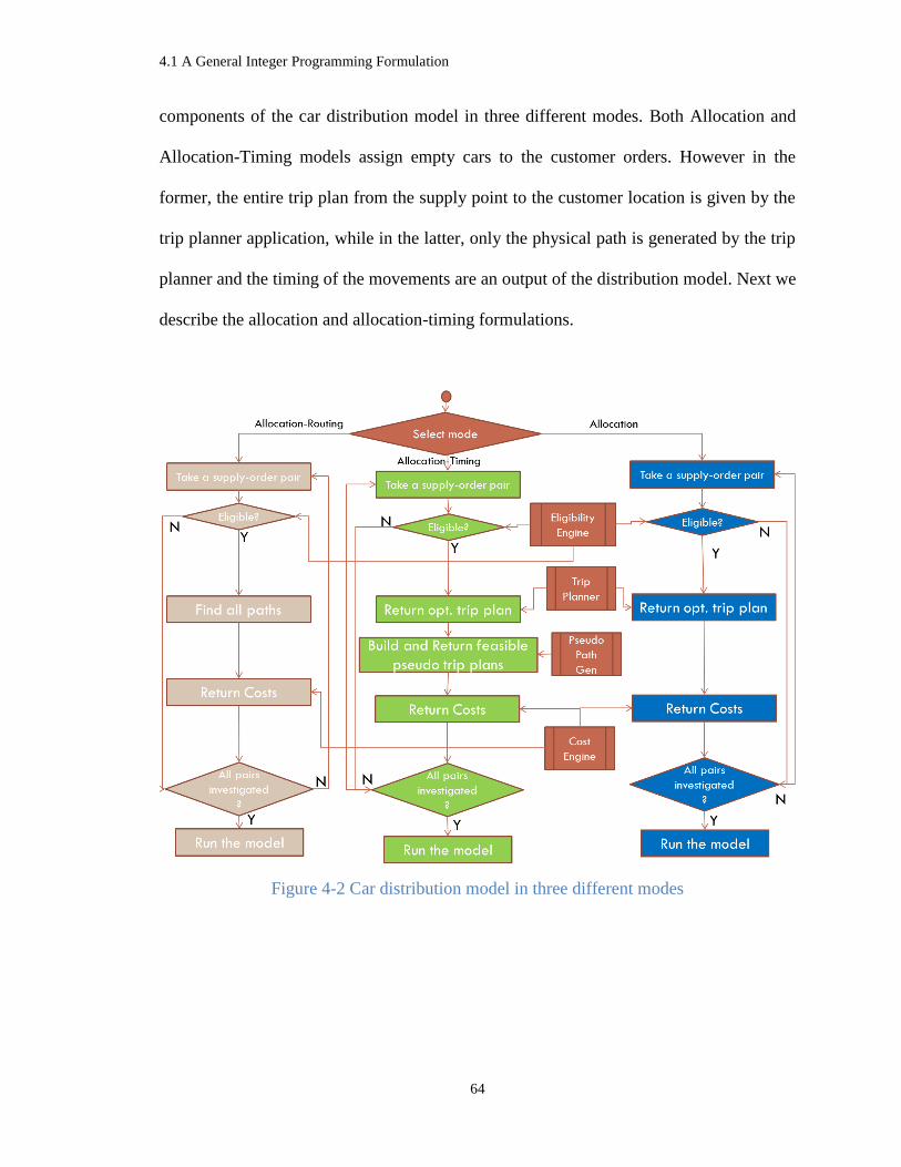
4.1 A General Integer Programming Formulation
64
components of the car distribution model in three different modes. Both Allocation and
Allocation-Timing models assign empty cars to the customer orders. However in the
former, the entire trip plan from the supply point to the customer location is given by the
trip planner application, while in the latter, only the physical path is generated by the trip
planner and the timing of the movements are an output of the distribution model. Next we
describe the allocation and allocation-timing formulations.
Figure 4-2 Car distribution model in three different modes

4.2 Pure Allocation Model on a Bipartite Resource Constrained Graph
65
4.2 Pure Allocation Model on a Bipartite Resource Constrained Graph
In railway industry, car routing and car distribution decisions are usually made
separately. Hence let us assume that an external application, say the trip planner, will
determine the optimal trip plan between every requested origin-destination pair. For
example, the trip planner suggests the green path 𝑏1T: g1T-𝑏2R: g2R for 𝑠2-𝑑 pair in Figure
4-3(a-1). The algorithm that delivers this path is an internal of the trip planner and is out
of the scope of the allocation model. Since there is at most one path between each origin-
destination pair, we can consider this path, in the time-space network, as an arc, in a
bipartite supply-demand graph, use blocks and trains involved in the path, as resources
(Figure 4-3(a-2)) and transform the problem to a resource-constrained generalized
transportation model. The transformation can be implemented as follows: replace each
supply node 𝑚 with |𝐾| nodes, corresponding to the |𝐾| commodities, and connect these
nodes to all demand nodes 𝑛, that were feasible to 𝑚, using arcs of length 𝑐𝑙𝑘.
Enforcing cars to flow on a single capacitated path from 𝑚 to 𝑛 or to have to choose
another destination might increase the total unmet demands or the overall assignment costs.
Example 4-1: Let us consider a network with only two supply nodes, one demand
node and one intermediate classification yard in Figure 4-3(a-1). The supply nodes 𝑠1 and
𝑠2 each has a surplus of two cars of the same pool and the demand node 𝑑 requires two
cars of a similar pool with a maximum delay of three days. Also assume that the path
𝑏3𝑇: 𝑔3𝑇 and path 𝑏1𝑇: 𝑔1𝑇-𝑏2𝑅: 𝑔2𝑅 are suggested by the trip planner as the optimal paths
for the 𝑠1- 𝑑 and 𝑠2- 𝑑 pairs respectively, where the assignment cost of the first path is
considerably higher than the second one and the unmet demand penalty is extremely high

4.2 Pure Allocation Model on a Bipartite Resource Constrained Graph
66
compared to the assignment cost. Let’s consider three scenarios and investigate the
behavior of our model.
Scenario 1: If there is no capacity limit (or a limit of more than two cars which will
make the capacity constraint to be redundant) on the arcs 𝑏1𝑇: 𝑔1𝑇 and 𝑏2𝑅: 𝑔2𝑅, then both
cars in 𝑠2 would be planned to 𝑑.
Scenario 2: But if arc 𝑏2𝑅: 𝑔2𝑅 has a capacity limit of one car then the previous
assignment will not be feasible anymore. The optimal solution will then be to send one car
from 𝑠1 and one car from 𝑠2, which apparently has a higher assignment cost than the first
scenario.
Scenario 3: Now let’s assume that arc 𝑏2𝑅: 𝑔2𝑅 has a capacity limit of one car and
arc 𝑏3𝑇: 𝑔3𝑇 is full. Then the optimal (and the only feasible) solution is to provide only one
car from 𝑠2, resulting in one unit of unmet demand.
Now let see what an experienced car dispatcher would traditionally, without using
a mathematical model, do in scenario 3. A car dispatcher will most likely not know about
the capacities of the network while making his decision. Based on his experience or a
simple judgment he would pick one of the two supply yards, let say yard 𝑠2, and will assign
the two cars available in that yard to the demand node. What happens next is more
interesting. Since arc 𝑏2𝑅: 𝑔2𝑅 has only one unit of capacity left, only one of the two cars
will make it to its destination by Saturday night. The second car however will not be able
to take 𝑏2𝑅: 𝑔2𝑅. So it will stay till there is an empty capacity available probably tomorrow!
The day after? As long as this car arrives to the customer before the order expiration date,
i.e. within three days delay, the performance of this dispatcher will beat our model's
solution. Order fulfillment ratio is an important performance measure for the distribution

4.2 Pure Allocation Model on a Bipartite Resource Constrained Graph
67
department and such an output of Scenario 3 is not acceptable! The reality is a pure
allocation model that takes a single path provided by the trip planner as the face value is
overseeing the dynamics of the service network and hence is not realistic. In the next
section we provide a way to include this dynamic into the model.

4.2 Pure Allocation Model on a Bipartite Resource Constrained Graph
68
Figure 4-3 An arc-train network with only one path between any O-D pair (a-1) can be
transformed to a resource-constrained bipartite graph (a-2), while the one with more than
one path (b-1) is transformed to a bipartite multigraph (b-2).

4.3 Allocation-Timing Model on a Bipartite Resource Constrained Multigraph
69
4.3 Allocation-Timing Model on a Bipartite Resource Constrained
Multigraph
In order to avoid the Pure Allocation models foible in ignoring the dynamics of the
service network, and at the same time avoiding combining the decisions that are made in
different departments, i.e. the car routing and car distribution decisions, we take the trip
plan’s suggested path as a basis and try to develop new paths by adding inventory and delay
arcs to it. In this research such paths that use the same physical path, i.e. blocks and trains,
to the ones in the trip plan but with different timings are referred to as pseudo trip-plans or
pseudo paths. The blue path and the green-red-blue path in Figure 4-3(b-1) are created
using such a procedure. The bipartite transformation of the block-train network after
introducing pseudo paths is a multigraph (Figure 4-3(b-2)).
After introducing the pseudo trip-plans, the optimal solution of Example 4-1 in
Section 4.2 is to send two cars from 𝑠2 to 𝑑, where one car is planned on path 𝑏1𝑇: 𝑔1𝑇-
𝑏2𝑅: 𝑔2𝑅 and another one is planned on path 𝑏1𝑇: 𝑔1𝑇-𝑏2𝐹: 𝑔2𝐹.
This path based formulation of empty railcars in which the paths connecting
feasible supply-demands are given by calling an external application (trip planner) but the
car distribution model is in charge of the optimal supply to demand allocation and the
timing of the movements, in this research is referred to as the Allocation-Timing model.
4.3.1 An Algorithm for Generating Pseudo-paths of a Trip plan
Before presenting our algorithm for finding all pseudo paths associated with a trip
plan, we recall the concept of lattice path in combinatorics and see how it is connected to
our algorithm. A lattice path 𝐿 in ℤ𝑑 of length 𝑘 with steps in 𝑆 is a sequence 𝑣0, 𝑣1, … , 𝑣𝑘 ∈
ℤ𝑑 such that each consecutive difference 𝑣𝑖 − 𝑣𝑖−1 lies in 𝑆 (Stanley, 2011). An example

4.3 Allocation-Timing Model on a Bipartite Resource Constrained Multigraph
70
of a lattice path in ℤ2 of length 4 with steps in 𝑆 = {(0,1), (1,0), (1,1)} is 𝐿 =
{(1,0), (1,1), (2,1), (3,2), (3,3)} and is illustrated in Figure 4-4.
Figure 4-4 Lattice path of length four in in ℤ𝟐
A North-Eastern (NE) lattice path is a path consisting of (1, 0) and (0, 1) steps,
where (1,0) steps are called East steps and denoted by E and (0,1) steps are called North
steps and denoted by N.
Figure 4-5 shows six NE paths originating from point (0,0). In fact there is no more
NE path with two E’s and two N’s originating from (0,0) in addition to these six paths.
And more strongly any NE path connecting (0,0) to (2,2) must have two N’s and two E’s.
NE lattice paths most commonly begin at the origin. This convention allows us to
encode all the information about a NE lattice path 𝐿 in a single permutation word. The
length of the word gives us the number of steps of the lattice path, 𝑘, and the order of
the N's and E's communicates the sequence of 𝐿. Furthermore, the number of N's and the
number of E's in the word determines the end point of 𝐿. 2
The set of all NE paths with 𝑎 steps of N and 𝑏 steps of E can be generated as the
set of all permutation of 𝑎 + 𝑏 items with 𝑎 identical items N and 𝑏 identical items E, or
simply saying the set of all words that can be written using 𝑎 times letter N and 𝑏 times
letter E. Size of such a set is (𝑎 + 𝑏𝑎
).
2 http://en.wikipedia.org/wiki/Lattice_path
(0,0)

4.3 Allocation-Timing Model on a Bipartite Resource Constrained Multigraph
71
Figure 4-5 Six lattice paths and their associated permutation words
Now let’s consider a case where trip planner has indicated that path 𝑏1𝑇 − 𝑏2𝑅 in
Figure 4-6(a) is optimal path between s and 𝑑. The problem of finding all pseudo paths
between s and 𝑑 is similar to finding all lattice paths between points (0,0) and (2,2). Path
𝑏1𝑇 − 𝑏2𝑅 can be encoded as IBIB, where I stands for inventory arc and B stands for block.
The five other paths can be listed as: IIBB, representing 𝑏1𝑊 − 𝑏2𝑅; BBII, representing
𝑏1𝑀 − 𝑏2𝑇; IBBI, representing 𝑏1𝑇 − 𝑏2𝑊, BIBI representing 𝑏1𝑀 − 𝑏2𝑊, and BIIB
representing 𝑏1𝑀 − 𝑏2𝑅. Furthermore let’s consider a case of Figure 4-6(b) where a
maximum delay of two days is acceptable by customer at demand node 𝑑. Then the
permutations should be generated using two more inventory arcs, IBIBII, resulting in 15
paths.
Next we develop a dynamic programming method to find all pseudo paths
associated with a given trip plan (path). A pseudocode of the major components of the
algorithm is presented here. The method returnAllPseudoPaths() takes a given path 𝑙 as
input and translates it to a word using PathToString() method. Then using another method,
returnListOfAllPermutations(), returns all words that are created using letters of this word.
Finally all these words are translated back to their associated paths, using StringToPath()
method, and the output is returned. Among the three inner methods (i.e. PathToString(),
returnListOfAllPermutations(), and StringToPath()), method returnListOfAllPermutations
as the main combinatorial part of the pseudo path generator is presented in detail.
(2,2)
(0,0)
NNEE NENE NEEN EENNENNEENEN

4.3 Allocation-Timing Model on a Bipartite Resource Constrained Multigraph
72
The returnListOfAllPermutations() reads a given word letter-by-letter. After
reading each letter, and before reading the next one, it generates all the words that can be
created using the substring traversed so far and save them in a set called currentSet. Similar
to other dynamic programming methods, at each step and after reading each letter, the
algorithm uses the substrings created before to generate new substrings of one size more.
The algorithm ends when all the letters are traversed. Example 4-2 illustrates how
returnListOfAllPermutations () works.

4.3 Allocation-Timing Model on a Bipartite Resource Constrained Multigraph
73
Pseudocode for generating all pseudo paths of a given path
returnAllPseudoPaths( Path l){
Array<Path> pseudoPathsList = new array();
String givenWord = PathToString(l);
Array<String> wordList = returnListOfAllPermutations(givenWord);
For (Each word In wordList){
Path pseudoPath = StringToPath(word);
pseudoPathsList.add(pseudoPath)
} Return pseudoPathsList;
}
Pseudocode for generating all permutations of a given word
returnListOfAllPermutations (Array<Char> givenWord) {
Set<Array<Char>> permutationsList = New Set();
Array<Char> start = New Array();
i = 1;
start[i] = givenWord[i];
permutationsList.Add(start);
for (i = 2; i <= givenWord.Length; i++) {
Set<Array<Char>> currentSet = new Set();
for (Each permutation In permutationsList) {
for (j = 1; j <= permutation.size() + 1; j++) {
Array<Char> newPermutation = permutation;
newPermutation.add(j, givenWord[i]);`
currentSet.add(newPermutation);
}
} permutationsList = currentSet;
}
return permutationsList;
}

4.3 Allocation-Timing Model on a Bipartite Resource Constrained Multigraph
74
Example 4-2) Generate all permutations of a givenWord = BIIB
givenWord = BIIB
permutationsList = {}, start = []
----------------
i=1 givenWord[i] = B
start = [B]
permutationsList = {[B]}
----------------
i=2 givenWord[i] = I
currentSet ={}
permutation = [B]
permutationsList ={[IB], [BI] }
----------------
i=3 givenWord[i] = I
currentSet ={}
permutationsList ={[IB], [BI] }
permutation = [IB]
permutation = [BI]
permutationsList ={[IIB], [IBI], [BII]} ----------------
i=4 givenWord[i] = B
currentSet ={}
permutationsList ={[IIB], [IBI], [BII]}
permutation = [IIB]
permutation = [IBI]
permutation = [BII]
permutationsList =
{[BIIB], [IBIB], [IIBB], [BIBI], [IBBI], [BBII]}
j newPerm currentSet
1 [IB] {[IB]}
2 [BI] {[IB], [BI] }
j newPerm currentSet
1 [IIB] {[IIB]}
2 [IIB] {[IIB]}
3 [IBI] {[IIB], [IBI]}
j newPerm currentSet
1 [IBI] {[IIB], [IBI]}
2 [BII] {[IIB], [IBI], [BII]}
3 [BII] {[IIB], [IBI], [BII]}
j newPerm currentSet
1 [BIIB] {[BIIB]}
2 [IBIB] {[BIIB], [IBIB]}
3 [IIBB] {[BIIB], [IBIB], [IIBB] }
4 [IIBB] {[BIIB], [IBIB], [IIBB] }
j newPerm currentSet
1 [BIBI] {[BIIB], [IBIB], [IIBB], [BIBI] }
2 [IBBI] {[BIIB], [IBIB], [IIBB], [BIBI], [IBBI]}
3 [IBBI] {[BIIB], [IBIB], [IIBB], [BIBI], [IBBI]}
4 [IBIB] {[BIIB], [IBIB], [IIBB], [BIBI], [IBBI]}
j newPerm currentSet
1 [BBII] {[BIIB], [IBIB], [IIBB], [BIBI], [IBBI], [BBII]}
2 [BBII] {[BIIB], [IBIB], [IIBB], [BIBI], [IBBI], [BBII]}
3 [BIBI] {[BIIB], [IBIB], [IIBB], [BIBI], [IBBI], [BBII]}
4 [BIIB] {[BIIB], [IBIB], [IIBB], [BIBI], [IBBI], [BBII]}

4.3 Allocation-Timing Model on a Bipartite Resource Constrained Multigraph
75
Figure 4-6. A trip plan and its associated pseudo paths when a) no delay is permitted, and
b) a maximum delay of two days is acceptable

4.3 Allocation-Timing Model on a Bipartite Resource Constrained Multigraph
76
4.3.2 A Lagrangian Heuristic
The path-based Allocation-Timing model is not easy to solve by integer
programming methods. This is why developing heuristic methods is needed. One method
could be a Lagrangian based heuristic by dualizing the capacity constraints and keeping
the supply and demand constraints as the main constraints. The algorithm is similar to the
one of Holmberg et al. (2008). The Lagrangian Relaxation is implemented by dualizing
constraint sets (4-15) and (4-16) as follows:
𝐿𝑅(𝛼, 𝛽) = 𝑚𝑖𝑛𝑥,𝑦,𝑧
[∑ (𝑓𝑏 − 𝛽𝑏𝑣𝑏)𝑧𝑏𝑏∈𝐵 + ∑ ∑ (𝑐𝑙𝑘 +𝑘∈𝐾,𝐾⊆𝛹𝑙∈𝐿
𝜔𝑘 ∑ 𝛼𝑔𝑔∈𝐺𝑙,𝐺𝑙={𝑔:𝑙∈𝐿𝑔} + 𝜏𝑘 ∑ 𝛽𝑏𝑏∈𝐵𝑙,𝐵𝑙={𝑏:𝑙∈𝐿𝐵} ) 𝑥𝑙
𝑘 +
∑ 𝑐𝑛 𝑦𝑛𝑛∈𝑁𝐾,𝐾⊆𝛹 − ∑ 𝛼𝑔𝑢𝑔𝑔∈𝐺 ]
s.t. (4-13), (4-14), (4-17), (4-18), (4-19), (4-20)
(4-21)
The Lagrangian function (4-21) can be decomposed into three components in (4-22),
among them one function, (4-23) to be optimized on z, and another one, (4-24), to be
optimized on x and y. The third component in (4-22) is a constant for a given vector 𝛼 and
does not need to be further considered.
𝐿𝑅(𝛼, 𝛽) = 𝐿𝑅1(𝛽) + 𝐿𝑅2(𝛼, 𝛽) − ∑ 𝛼𝑔𝑢𝑔𝑔∈𝐺 (4-22)
𝐿𝑅1(𝛽) = 𝑚𝑖𝑛𝑧(∑ (𝑓𝑏 − 𝛽𝑏𝑣𝑏)𝑧𝑏𝑏∈𝐵 ) 𝑠. 𝑡. (4-20) (4-23)
𝐿𝑅2(𝛼, 𝛽) = 𝑚𝑖𝑛𝑥,𝑦
(∑ ∑ (𝑐𝑙𝑘 + 𝜔𝑘 ∑ 𝛼𝑔𝑔∈𝐺𝑙,𝐺𝑙={𝑔:𝑙∈𝐿𝑔}
+𝑘∈𝐾,𝐾⊆𝛹𝑙∈𝐿
𝜏𝑘 ∑ 𝛽𝑏𝑏∈𝐵𝑙,𝐵𝑙={𝑏:𝑙∈𝐿𝐵} )𝑥𝑙𝑘 + ∑ 𝑐𝑛 𝑦𝑛𝑛∈𝑁𝐾,𝐾⊆𝛹 )
s.t. (4-13), (4-14), (4-17), (4-18), (4-19)
(4-24)
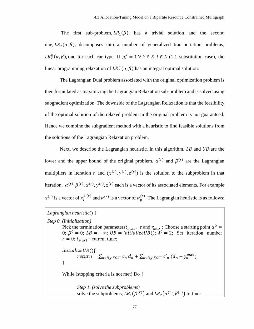
4.3 Allocation-Timing Model on a Bipartite Resource Constrained Multigraph
77
The first sub-problem, 𝐿𝑅1(𝛽), has a trivial solution and the second
one, 𝐿𝑅2(𝛼, 𝛽), decomposes into a number of generalized transportation problems,
𝐿𝑅2𝐾(𝛼, 𝛽), one for each car type. If 𝜇𝑙
𝑘 = 1 ∀ 𝑘 ∈ 𝐾, 𝑙 ∈ 𝐿 (1:1 substitution case), the
linear programming relaxation of 𝐿𝑅2𝐾(𝛼, 𝛽) has an integral optimal solution.
The Lagrangian Dual problem associated with the original optimization problem is
then formulated as maximizing the Lagrangian Relaxation sub-problem and is solved using
subgradient optimization. The downside of the Lagrangian Relaxation is that the feasibility
of the optimal solution of the relaxed problem in the original problem is not guaranteed.
Hence we combine the subgradient method with a heuristic to find feasible solutions from
the solutions of the Lagrangian Relaxation problem.
Next, we describe the Lagrangian heuristic. In this algorithm, 𝐿𝐵 and 𝑈𝐵 are the
lower and the upper bound of the original problem. 𝛼(𝑟) and 𝛽(𝑟) are the Lagrangian
multipliers in iteration 𝑟 and (𝑥(𝑟), 𝑦(𝑟), 𝑧(𝑟)) is the solution to the subproblem in that
iteration. 𝛼(𝑟), 𝛽(𝑟), 𝑥(𝑟), 𝑦(𝑟), 𝑧(𝑟) each is a vector of its associated elements. For example
𝑥(𝑟) is a vector of 𝑥𝑙𝑘,(𝑟)
and 𝛼(𝑟) is a vector of 𝛼𝑔(𝑟)
. The Lagrangian heuristic is as follows:
Lagrangian heuristic() {
Step 0. (Initialization)
Pick the termination parameters𝑡𝑚𝑎𝑥 , 𝜀 and 𝑟𝑚𝑎𝑥 ; Choose a starting point 𝛼0 =0; 𝛽0 = 0; 𝐿𝐵 = −∞; 𝑈𝐵 = 𝑖𝑛𝑖𝑡𝑖𝑎𝑙𝑖𝑧𝑒𝑈𝐵(); 𝜆0 = 2; Set iteration number
𝑟 = 0; 𝑡𝑠𝑡𝑎𝑟𝑡= current time;
𝑖𝑛𝑖𝑡𝑖𝑎𝑙𝑖𝑧𝑒𝑈𝐵(){ 𝑟𝑒𝑡𝑢𝑟𝑛 ∑ 𝑐𝑛 𝑑𝑛𝑛∈𝑁𝐾,𝐾⊆𝛹 + ∑ 𝑐′𝑛 (𝑑𝑛 −𝑛∈𝑁𝐾,𝐾⊆𝛹, 𝑦𝑛
𝑚𝑎𝑥)
}
While (stopping criteria is not met) Do {
Step 1. (solve the subproblems)
solve the subproblems, 𝐿𝑅1(𝛽(𝑟)) and 𝐿𝑅2(𝛼
(𝑟), 𝛽(𝑟)) to find:
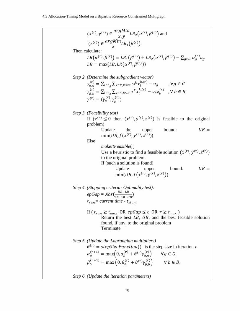
4.3 Allocation-Timing Model on a Bipartite Resource Constrained Multigraph
78
(𝑥(𝑟), 𝑦(𝑟)) ∈𝑎𝑟𝑔𝑀𝑖𝑛𝑥, 𝑦
𝐿𝑅2(𝛼(𝑟), 𝛽(𝑟)) and
(𝑧(𝑟)) ∈𝑎𝑟𝑔𝑀𝑖𝑛
𝑧𝐿𝑅1(𝛽
(𝑟)).
Then calculate:
𝐿𝑅(𝛼(𝑟), 𝛽(𝑟)) = 𝐿𝑅1(𝛽(𝑟)) + 𝐿𝑅2(𝛼
(𝑟), 𝛽(𝑟)) − ∑ 𝛼𝑔(𝑟)𝑢𝑔𝑔∈𝐺
𝐿𝐵 = max {𝐿𝐵, 𝐿𝑅(𝛼(𝑟), 𝛽(𝑟))}
Step 2. (Determine the subgradient vector)
𝛾𝛼,𝑔(𝑟)= ∑ ∑ 𝜔𝑘𝑥𝑙
𝑘,(𝑟)𝑘∈𝐾,𝐾⊆𝛹𝑙∈𝐿𝑔 − 𝑢𝑔 , ∀𝑔 ∈ 𝐺
𝛾𝛽,𝑏(𝑟)= ∑ ∑ 𝜏𝑘𝑥𝑙
𝑘,(𝑟)𝑘∈𝐾,𝐾⊆𝛹𝑙∈𝐿𝑏 − 𝑣𝑏𝑧𝑏
(𝑟) , ∀ 𝑏 ∈ 𝐵
𝛾(𝑟) = (𝛾𝛼(𝑟), 𝛾𝛽(𝑟))
Step 3. (Feasibility test)
If (𝛾(𝑟) ≤ 0 then (𝑥(𝑟), 𝑦(𝑟), 𝑧(𝑟)) is feasible to the original
problem)
Update the upper bound: 𝑈𝐵 =min (𝑈𝐵, 𝑓(𝑥(𝑟), 𝑦(𝑟), 𝑧(𝑟)))
Else
makeItFeasible( )
Use a heuristic to find a feasible solution (�̅�(𝑟), �̅�(𝑟), 𝑧̅(𝑟)) to the original problem.
If (such a solution is found)
Update upper bound: 𝑈𝐵 =
min (𝑈𝐵, 𝑓(�̅�(𝑟), �̅�(𝑟), 𝑧̅(𝑟)))
Step 4. (Stopping criteria- Optimality test):
epGap = 𝐴𝑏𝑠(𝑈𝐵−𝐿𝐵
1𝑒−10+𝑈𝐵)
𝑡𝑟𝑢𝑛= current time - 𝑡𝑠𝑡𝑎𝑟𝑡
If ( 𝑡𝑟𝑢𝑛 ≥ 𝑡𝑚𝑎𝑥 OR 𝑒𝑝𝐺𝑎𝑝 ≤ 𝜀 OR 𝑟 ≥ 𝑟𝑚𝑎𝑥 )
Return the best 𝐿𝐵, 𝑈𝐵, and the best feasible solution
found, if any, to the original problem
Terminate
Step 5. (Update the Lagrangian multipliers)
𝜃(𝑟) = 𝑠𝑡𝑒𝑝𝑆𝑖𝑧𝑒𝐹𝑢𝑛𝑐𝑡𝑖𝑜𝑛() is the step size in iteration 𝑟
𝛼𝑔(𝑟+1)
= max(0, 𝛼𝑔(𝑟) + 𝜃(𝑟)𝛾𝛼,𝑔
(𝑟)) ∀𝑔 ∈ 𝐺,
𝛽𝑏(𝑛+1)
= max (0, 𝛽𝑏(𝑟) + 𝜃(𝑟)𝛾𝛽,𝑏
(𝑟)) ∀ 𝑏 ∈ 𝐵,
Step 6. (Update the iteration parameters)

4.3 Allocation-Timing Model on a Bipartite Resource Constrained Multigraph
79
𝑢𝑝𝑑𝑎𝑡𝑒𝐿𝑎𝑚𝑏𝑑𝑎(ℎ) 𝑟 = 𝑟 + 1
}
}
The Algorithm starts with initializing the parameters and setting up the termination
rules in Step 0. In Step 1 subproblems are solved and the lower and upper bounds on the
original problem are updated accordingly. In Step 2 the amount of residual capacity of
blocks and trains or their violation level, if overbooked, are calculated and the subgradient
vector is reported. If all elements of the subgradient vector are nonnegative, Step 3
identifies the current solution as a feasible solution; otherwise, it uses another heuristic,
called makeItFeasible which is presented latter in this section, to create a feasible solution
out of this infeasible solution. Any time a feasible solution is identified or created the upper
bound is updated. If none of the stopping criteria are met in Step 4, the Lagrangian
multipliers will be calculated in Step 5 and a new iteration will be performed starting from
Step 1. Parameter 𝜃(𝑟) in Step 5 is called step size in 𝑟th iteration and a trade-off between
the convergence time and solution precision should be considered while appointing a value
to it. A too small value for the step size might result in a long running time since the
algorithm might stuck in the current solution and does not converge, while a too large value
for it might increase the chance of overshooting the optimal solution or it may result in a
zigzag behavior between non optimal solutions. As mentioned in Ahuja et al. (1993) a
balance between the time and precision can be achieved if using a nonsummable
diminishing strategy:
𝜃(𝑟) ≥ 0, lim𝑟→∞
𝜃(𝑟) = 0, ∑ 𝜃(𝑟)∞𝑟=0 = ∞ (4-25)

4.3 Allocation-Timing Model on a Bipartite Resource Constrained Multigraph
80
Two step size setup strategies are presented here and both satisfy these conditions
(Ahuja et al., 1993). The first strategy, called a constant step size strategy, uses the reverse
of the iteration parameter (𝑟 ≥ 1) as step size and is presented as:
𝑠𝑡𝑒𝑝𝑆𝑖𝑧𝑒𝐹𝑢𝑛𝑐𝑡𝑖𝑜𝑛1() {
𝜃(𝑟) = 1/𝑟 }
The second strategy adapted from “Newton’s Method” for solving systems of
nonlinear equations employs the current bounds of the original problem as well as the
Euclidean norm of the subgradient vector to assign the step size.
𝑠𝑡𝑒𝑝𝑆𝑖𝑧𝑒𝐹𝑢𝑛𝑐𝑡𝑖𝑜𝑛2() {
𝜃(𝑟) =𝜆(𝑟)(𝑈𝐵 − 𝐿𝑅(𝛼(𝑟), 𝛽(𝑟))
‖𝛾‖2
}
where λ(r) is an scalar strictly between 0 and 2, initially set to 2 and updated, using
𝑢𝑝𝑑𝑎𝑡𝑒𝐿𝑎𝑚𝑏𝑑𝑎(ℎ) procedure, if the lower bound is not improved for a given number of
ℎ iterations:
𝑢𝑝𝑑𝑎𝑡𝑒𝐿𝑎𝑚𝑏𝑑𝑎(ℎ) {
If (𝐿𝐵 has not improved for ℎ iterations)
𝜆𝑛+1 = 𝜆𝑛/2 Else
𝜆𝑛+1 = 𝜆𝑛 }
As it comes from its name, makeItFeasible() Algorithm takes an infeasible solution
as an input and makes it feasible! The only constraints expected to be violated are the block
and train capacity constraints as we have relaxed them in the Lagrangian Relaxation

4.3 Allocation-Timing Model on a Bipartite Resource Constrained Multigraph
81
method. The violation level, or the amount by which the capacity is violated, are already
on hand, 𝛾𝛼,𝑔(𝑟) > 0 for train 𝑔 and 𝛾𝛽,𝑏
(𝑟) > 0 for block 𝑏. There might be many ways to alter
the current solution in order to obtain a feasible solution. Here we use an optimization
approach for this purpose.
makeItFeasible(𝑥(𝑟), 𝑦(𝑟), 𝑧(𝑟) ) {
1) calculate the flow reductions
Find the minimum number of changes in assignment variables that
resolve the violation of capacity constraints
𝐿𝐾 = {(𝑙, 𝑘): 𝑙 ∈ 𝐿, 𝑘 ∈ 𝐾,𝐾 ⊆ 𝛹, 𝑥𝑙𝑘 >
0 𝑖𝑛 𝑐𝑢𝑟𝑟𝑒𝑛𝑡 𝑖𝑛𝑓𝑒𝑎𝑠𝑖𝑏𝑙𝑒 𝑠𝑜𝑙𝑢𝑡𝑖𝑜𝑛 𝑜𝑓 𝐿𝑅}
min ∑ ∆𝑥𝑙𝑘
(𝑙,𝑘)∈𝐿𝐾
∗ 𝑐′𝑙𝑘 (4-26)
∑ ∆𝑥𝑙𝑘
(𝑙,𝑘)∈𝐿𝐾
∗ 𝜏𝑘 ≥ 𝛾𝛽,𝑏(𝑟) ∀ 𝑏 ∈ 𝐵, 𝛾𝛽,𝑏
(𝑟)> 0 (4-27)
∑ ∆𝑥𝑙𝑘
(𝑙,𝑘)∈𝐿𝐾
∗ 𝜔𝑘 ≥ 𝛾𝛼,𝑔(𝑟)
∀ 𝑔 ∈ 𝐺, 𝛾𝛼,𝑔(𝑟)> 0 (4-28)
0 ≤ ∆𝑥𝑙𝑘 ≤ 𝑥𝑙
𝑘 ∀ (𝑙, 𝑘) ∈ 𝐿𝐾 (4-29)
2) Update the decision variables
Update assignment variables
𝑥𝑙𝑘 = 𝑥𝑙
𝑘 − ∆𝑥𝑙𝑘
Then update the shortage variables and block construction variables
accordingly
𝑦𝑛 = 𝑑𝑛 − ∑ ∑ 𝜇𝑙𝑘𝑥𝑙
𝑘𝑘∈𝐾𝑛𝑙∈𝐿𝑛
𝑑 ∀ 𝑛 ∈ 𝑁𝐾, ∀ 𝐾 ⊆ 𝛹
𝑦′𝑛 = max( 𝑦𝑛 − 𝑦𝑛𝑚𝑎𝑥 , 0) ∀ 𝑛 ∈ 𝑁𝐾, ∀ 𝐾 ⊆ 𝛹
If ∃(𝑙, 𝑘) , 𝑙 ∈ 𝐿𝑏 𝑎𝑛𝑑 𝑥𝑙𝑘 > 0 then 𝑧𝑏 = 1; else 𝑧𝑏 = 0 , ∀ 𝑏 ∈ 𝐵
3) Return the feasible solution (�̅�(𝑟), �̅�(𝑟), 𝑧̅(𝑟))
}
Let’s assume that for a given (𝑙, 𝑘) the assignment variable 𝑥𝑙𝑘 has a positive value
and since the flow variables are integral 𝑥𝑙𝑘 ≥ 1. Furthermore let’s assume that the
coefficients, 𝜔𝑘or 𝜏𝑘, of this variable in some of the violated constraints is nonzero.

4.3 Allocation-Timing Model on a Bipartite Resource Constrained Multigraph
82
Apparently reducing 𝑥𝑙𝑘 by a value of one will help the violated constraints to be closer to
becoming a feasible solution. For example, if there are only three violated constraints all
with a violation level of one and the coefficient of 𝑥𝑙𝑘 in two of them is one, then one unit
reduction in 𝑥𝑙𝑘 will save two constraints from infeasibility. In general we prefer to make
as less change as possible during makeItFeasible() process assuring that demand
fulfillment ratio will not be dramatically affected.
The decision variable ∆𝑥𝑙𝑘 is the number of cars to be deducted from current value
𝑥𝑙𝑘. The objective function (4-26) tends to minimize the total deduction amount. The cost
coefficients of the objective function here have reverse relations with the ones in the
original problem. For example 𝑐′𝑙𝑘 =
1
𝑙𝑜𝑔𝑐𝑙𝑘 will assure that small cost coefficients 𝑐′𝑙
𝑘 are
assigned to the paths with high assignment costs 𝑐𝑙𝑘 in the original problem, practically
making their flow reduction more likely. While such a function might look intuitive, it
oversees the trade-off between assignment cost and unmet demand penalty and might
increase the overall cost. This is why we use a constant coefficient 𝑐′𝑙𝑘 = 1 that simply
minimizes the total flow change. Constraints (4-27) and (4-28) insure that the total change
in the flow is at least equal to the violation level while Constraint (4-29) states that the
change in flow cannot be more than the flow!
Another way to find the Lagrangian multipliers is to use Dantzig-Wolfe
Decomposition technique by defining the master problem on the bundle resource
consumption constraints (4-15) and (4-16) and defining one sub-problem for each
commodity over the supply-demand conservation constraint sets (4-13) and (4-14) for that
commodity. One important advantage of the Dantzig-Wolfe decomposition which
distinguishes it from other Lagrangian-based algorithms is that: In each iteration in addition

4.3 Allocation-Timing Model on a Bipartite Resource Constrained Multigraph
83
to providing a lower bound, it always maintains a feasible solution for the problem.
However, this algorithm is usually not as time-efficient as the subgradient method (Ahuja
et al., 1993).
4.3.3 An Iterative Relaxation and Rounding Heuristic
The decision variables of the PathBased formulation developed at Section 4.1 have
some interesting properties:
Property 4-1 The decision variables associated with the shortage (i.e. 𝑦𝑛) are dependent
variables and given the value of assignment variables (i.e. 𝑥𝑙𝑘) their values can be
calculated.
Property 4-2 The decision variables associated with the critical shortage (i.e. y′n) are
dependent variables and given the value of shortage variables (i.e. 𝑦𝑛) their values can be
calculated.
Property 4-3 The design variables associated with the block setups (i.e. 𝑧𝑏) are dependent
variables and given the value of assignment variables (i.e. 𝑥𝑙𝑘) their values can be
calculated.
Based on Property 4-1 to Property 4-3 if the values of the assignment variables (i.e.
𝑥𝑙𝑘) are given, the values of the rest of the variables can be calculated and the objective
function can be evaluated. Another observation from this model is that:
Property 4-4 The optimal solution, and more generally any feasible solution of the LP
Relaxation of the PathBased formulation, after dropping the fractional parts of the decision
variables and updating the rest of variables, is feasible to the original PathBased model.

4.3 Allocation-Timing Model on a Bipartite Resource Constrained Multigraph
84
Property 4-4 always holds since a decision of even not satisfying any order is feasible to
the model, although not desirable and definitely not optimal because of high shortage
penalties. Hence any decrease in the assignment variables, as long as doesn’t make them
negative, is feasible to the model but only after updating the shortage variables and block
setup variables according to the changes. This interesting property opens up a variety of
approximation techniques to us.
An easy, and probably the most common, approach to the IP problems is the
Rounding technique. The rounding approach solves the linear relaxation of the IP problem
and attempts to round the solution to an integer one by dropping all the fractional parts of
the decision variables or by finding satisfactory solutions wherein the variable values are
adjusted to close larger or smaller integer values.
Another way of dealing with Integer programs is Iterative Algorithm first
introduced by Jain (2001) in solving the survivable network design problem. This
technique benefits from properties of extreme point solutions through an iterative
algorithm. At each iteration a subset of variables is rounded. Then, the constraints are
modified to reflect the residual problem based on the rounded variables. Such an updated
instance is passed to the next iteration for further processing.
In this research we develop an approximation iterative method based on
consecutive relaxation and rounding as follows:
Iterative Relaxation and Rounding Heuristic (IRRH)
1- Call the PathBased formulation as Original IP problem (OIP) with decision
variables (𝑥, 𝑦, 𝑦′, 𝑧), where each element is a vector by itself, e.g. 𝑥 is a vector of
assignment variables 𝑥𝑙𝑘. Let (𝑥∗, 𝑦∗, 𝑦′∗, 𝑧∗) be OIP’s optimal solution to be discovered.
Set (𝑥∗, 𝑦∗, 𝑦′∗, 𝑧∗) to (0,0,0,0)
2- CurrentIPProblem = OIP
3- Relax the integrality constraints of CurrentIPProblem and solve the LP

4.3 Allocation-Timing Model on a Bipartite Resource Constrained Multigraph
85
Relaxation (LPR) to optimality. Let (𝑋∗, 𝑌∗, 𝑌′∗, 𝑍∗) be the optimal solution of LPR
4- Update the assignment variables of OIP using 𝑥𝑙∗𝑘+= 𝑅𝑜𝑢𝑛𝑑𝐷𝑜𝑤𝑛(𝑋𝑙
∗𝑘) 5- Update the rest of OIP variables based on (4-30), (4-31), and (4-32):
𝑦∗𝑛= 𝑑𝑛 − ∑ ∑ 𝜇𝑙
𝑘𝑥𝑙∗𝑘
𝑘∈𝐾𝑛𝑙∈𝐿𝑛𝑑 (4-30)
𝑦′∗𝑛= max(0, 𝑦∗
𝑛− 𝑦𝑛
𝑚𝑎𝑥) (4-31)
𝑧∗𝑏 = {1 𝑖𝑓 ∃𝑙 ∈ 𝐿𝑏 , 𝑥𝑙
∗𝑘 > 00 𝑜𝑡ℎ𝑒𝑟𝑤𝑖𝑠𝑒
(4-32)
6- If stopping criteria is met
Return the optimal solution (𝑥∗, 𝑦∗, 𝑦′∗, 𝑧∗) and objective value
Else
Introduce a new problem called IP Residual (IPR). IPR has the same
formulation of OIP but on residual parameters noted by CAPITAL case
letters (e.g. 𝐹𝑏 in IPR is the block setup cost similar to 𝑓𝑏 in OIP). Calculate
the parameters of IPR based on equations (4-33) to (4-38).
𝐹𝑏 = {0 𝑖𝑓 𝑧∗𝑏 = 1𝑓𝑏 𝑜𝑡ℎ𝑒𝑟𝑤𝑖𝑠𝑒
(4-33)
𝑆𝑚𝑘 = 𝑠𝑚
𝑘 − ∑ 𝑥𝑙∗𝑘
𝑙∈𝐿𝑚𝑜 (4-34)
𝐷𝑛 = 𝑦∗𝑛 (4-35)
𝑌𝑛𝑚𝑎𝑥 = {
𝑦∗𝑛 𝑖𝑓 𝑦∗𝑛 ≤ 𝑦𝑛𝑚𝑎𝑥
𝑦𝑛𝑚𝑎𝑥 𝑜𝑡ℎ𝑒𝑟𝑤𝑖𝑠𝑒
(4-36)
𝑈𝑔 = 𝑢𝑔 − ∑ ∑ 𝜔𝑘𝑥𝑙∗𝑘
𝑘∈𝐾,𝐾⊆𝛹𝑙∈𝐿𝑔 (4-37)
𝑉𝑏 = 𝑣𝑏 − ∑ ∑ 𝜏𝑘𝑥𝑙∗𝑘
𝑘∈𝐾,𝐾⊆𝛹𝑙∈𝐿𝑏 (4-38)
CurrentIPProblem = IPR
Go to step 3
The stopping criteria might be time or number of iterations. The relaxation in Step 3
of the iterative algorithm can be performed in two ways: a) we can relax only the integer
variables and keep the binary ones as it is (IRRH1) or b) we can relax all integer variables
to general non negative variables and relax all binary variables to continuous variables
between 0 and 1 (IRRH2).

4.4 Noncapacitated Model and its Optimistic Behavior on a Capacitated Network
86
4.4 Noncapacitated Model and its Optimistic Behavior on a Capacitated
Network
As part of our validation procedure, and as it will be discussed later in Chapter 6,
we compare the performance of our model with the noncapacitated model’s performance.
However in order to be able to benchmark our model against the noncapacitated model, we
need to recalculate the performance measure of this model in a capacitated network, simply
saying to compare apples with apples and not with oranges!
First let us start with the formulation of a noncapacitated model. The objective of
current noncapacitated models is usually to minimize the total assignment costs plus the
shortage cost without considering the block setup costs. Regarding the constraints,
everything is the same as the path-based Pure Allocation model except that capacity
constraints for blocks and trains are relaxed. Objective function (4-39) along with the
supply limitation (4-40), demand satisfaction (4-41), soft service level (4-42) and the
variable type constraints (4-43)-(4-44) constitute the noncapacitated model formulation as
follows (see Table 4-1 for the notation and Section 4.1 for the details on the constraints):
NC (see Table 4-1for the notations):
𝑀𝑖𝑛 ∑ ∑ 𝑐𝑙𝑘 𝑥𝑙
𝑘𝑘∈𝐾,𝐾⊆𝛹𝑙∈𝐿 + ∑ 𝑐𝑛 𝑦𝑛𝑛∈𝑁𝐾,𝐾⊆𝛹 + ∑ 𝑐′𝑛 𝑦′𝑛𝑛∈𝑁𝐾,𝐾⊆𝛹 (4-39)
∑ 𝑥𝑙𝑘 ≤ 𝑠𝑚
𝑘𝑙∈𝐿𝑚
𝑜 ∀ 𝑚 ∈ 𝑀,∀𝑘 ∈ 𝐾 ⊆ 𝛹 (4-40)
∑ ∑ 𝜇𝑙𝑘𝑥𝑙
𝑘𝑘∈𝐾𝑛𝑙∈𝐿𝑛
𝑑 + 𝑦𝑛 = 𝑑𝑛 ∀ 𝑛 ∈ 𝑁𝐾, 𝐾 ⊆ 𝛹 (4-41)
𝑦′𝑛 ≥ 𝑦𝑛 − 𝑦𝑛𝑚𝑎𝑥 ∀ 𝑛 ∈ 𝑁𝐾, ∀ 𝐾 ⊆ 𝛹 (4-42)
𝑥𝑙𝑘 ≥ 0 𝑎𝑛𝑑 𝑖𝑛𝑡𝑒𝑔𝑒𝑟
∀𝑙 ∈ 𝐿, ∀𝑘 ∈ 𝐾,𝐾 ⊆
𝛹
(4-43)
4.4 Noncapacitated Model and its Optimistic Behavior on a Capacitated Network
87
𝑦𝑛, 𝑦′𝑛 ≥ 0 ∀ 𝑛 ∈ 𝑁𝐾, ∀ 𝐾 ⊆ 𝛹 (4-44)
Property 4-5 The objective value of noncapacitated model NC is always at least as good
as the Pure Allocation PA and the Allocation-Timing AT models.
Property 4-5 always holds since the feasible region of a NC, as a result of relaxing
the capacity constraints, is a superset of the PA’s. Feasible region of NC and AT models
can’t be compared directly since one has more arcs and the other one has more capacities.
However since the single arc connecting a given supply-order pair in NC has the shortest
cost among all pseudo arcs connecting these nodes in AT and at the same time has an
infinite capacity on it; the objective value of NC will always be at least as good as AT, and
as a result at least as good as PA. In addition to the feasible region size and capacities,
absence of block setup costs in NC will potentially make the cost even lesser.
A direct conclusion of Property 4-5 is that benchmarking AT and PA models
against NC is pointless since the latter always holds a lesser objective value. Now let us
consider a case that the NC’s output has been used for car distribution planning in a network
that is actually capacitated. Since NC oversees the capacity limits while planning, it is
expected to see a gap between the actual implementation and the plan. The gap we are
addressing here is the gap solely caused as a result of ignoring the capacities while the
stochasticity of other parameters such as travel time, etc. is an unrelated issue. In order to
compare the performance of capacitated models AT and PA against current uncapacitated
model NC, we should design our benchmark based on the behavior of the uncapacitated
model in a capacitated network which will be denoted as NCActual. Such behavior can be
quantified, on average, by generating random problem instances and comparing the results.

4.4 Noncapacitated Model and its Optimistic Behavior on a Capacitated Network
88
However in this research we formulate a mathematical model that reports the optimistic
behavior of noncapacitated model in a capacitated network. Our goal is to show that the
performance of our model is better than the optimistic behavior of the NC in a capacitated
network and as a result is better than its average case behavior. The optimistic behavior
happens when the actual flow of cars will be in compliance with the assignment costs.
NCActual:
𝑀𝑖𝑛 ∑ 𝑓𝑏𝑧𝑏𝑏∈𝐵 + ∑ ∑ 𝑐𝑙′𝑘 𝑥𝑙′
𝑘𝑘∈𝐾,𝐾⊆𝛹𝑙′∈𝐿𝑝𝑠𝑒𝑢𝑑𝑜 + ∑ 𝐵𝑖𝑔𝑐𝑛 𝑦𝑛𝑛∈𝑁𝐾,𝐾⊆𝛹 +
∑ 𝐵𝑖𝑔𝑐′𝑛 𝑦′𝑛𝑛∈𝑁𝐾,𝐾⊆𝛹
(4-45)
∑ 𝑥𝑙′𝑘 + 𝑥′𝑙
𝑘 = 𝑙′∈𝐿𝑝𝑠𝑒𝑢𝑑𝑜(𝑙) 𝑥∗𝑙𝑘 ∀(𝑙, 𝑘), where flow of 𝑘 on 𝑙 is feasible
to NC
(4-46)
∑ ∑ 𝜇𝑙′𝑘𝑥𝑙′
𝑘𝑘∈𝐾𝑛𝑙′∈𝐿𝑝𝑠𝑒𝑢𝑑𝑜𝑛
𝑑 + 𝑦𝑛 = 𝑑𝑛 ∀ 𝑛 ∈ 𝑁𝐾, ∀ 𝐾 ⊆ 𝛹 (4-47)
𝑦′𝑛 ≥ 𝑦𝑛 − 𝑦𝑛𝑚𝑎𝑥 ∀ 𝑛 ∈ 𝑁𝐾, ∀ 𝐾 ⊆ 𝛹 (4-48)
∑ ∑ 𝜔𝑘𝑥𝑙′𝑘
𝑘∈𝐾,𝐾⊆𝛹𝑙′∈𝐿𝑔𝑝𝑠𝑒𝑢𝑑𝑜 ≤ 𝑢𝑔 ∀𝑔 ∈ 𝐺 (4-49)
∑ ∑ 𝜏𝑘𝑥𝑙′𝑘
𝑘∈𝐾,𝐾⊆𝛹𝑙′∈𝐿𝑏𝑝𝑠𝑒𝑢𝑑𝑜 ≤ 𝑣𝑏𝑧𝑏 ∀ 𝑏 ∈ 𝐵 (4-50)
𝑥𝑙′𝑘 ≥ 0 𝑎𝑛𝑑 𝑖𝑛𝑡𝑒𝑔𝑒𝑟 ∀𝑙′ ∈ 𝐿𝑝𝑠𝑒𝑢𝑑𝑜 , ∀𝑘 ∈ 𝐾,𝐾 ⊆ 𝛹 (4-51)
𝑥′𝑙𝑘 ≥ 0 ∀ 𝑙 ∈ 𝐿, ∀𝑘 ∈ 𝐾, ∀ 𝐾 ⊆ 𝛹 (4-52)
𝑦𝑛, 𝑦′𝑛 ≥ 0 ∀ 𝑛 ∈ 𝑁𝐾, ∀ 𝐾 ⊆ 𝛹 (4-53)
𝑧𝑏 ∈ {0,1} ∀𝑏 ∈ 𝐵 (4-54)
In this formulation 𝑙 ∈ 𝐿 is the path between the associated supply-order pair in NC
while 𝐿𝑝𝑠𝑒𝑢𝑑𝑜(𝑙) is a set containing all pseudo paths associated with 𝑙. The elements of
such set is denoted by 𝑙′. Consequently, 𝐿𝑔𝑝𝑠𝑒𝑢𝑑𝑜
, 𝐿𝑏𝑝𝑠𝑒𝑢𝑑𝑜
, 𝐿𝑝𝑠𝑒𝑢𝑑𝑜𝑛𝑑
, and 𝐿𝑝𝑠𝑒𝑢𝑑𝑜 represent

4.4 Noncapacitated Model and its Optimistic Behavior on a Capacitated Network
89
the updated version of sets 𝐿𝑔, 𝐿𝑏 , 𝐿𝑛𝑑 , and 𝐿 after adding the pseudo paths. Practically 𝐿
here is equal to 𝐿 in NC (and AP) while 𝐿𝑝𝑠𝑒𝑢𝑑𝑜is equal to 𝐿 in AT.
The decision variable of NCActual 𝑥𝑙′𝑘 is the number of cars of pool 𝑘 that will
actually flow on pseudo path 𝑙′. The definition of unmet demand variables 𝑦𝑛, 𝑦′𝑛 are the
same as the ones in NC. In addition to that, 𝑥′𝑙𝑘 is a new variable representing the overflow
of the NC output in a capacitated network. The shortage penalties, i.e. 𝐵𝑖𝑔𝑐𝑛 and 𝐵𝑖𝑔𝑐′𝑛,
in NCActual are not necessarily equal to the ones in NC (or Pure Allocation and Allocation-
Timing) model(s), i.e. 𝑐𝑛 and 𝑐′𝑛. NC, Pure Allocation and Allocation-Timing models, are
designed to help the decision maker while making the car distribution planning decisions;
hence the trade-off between assignment costs and shortage penalties are important and the
penalties should be well designed to guarantee that high cost assignments are avoided if
the shortage penalties are less than the assignment costs. On the other hand, the goal of
NCActual is to simulate the output of a noncapacitated model in a capacitated network and
not to make a decision. The trade-off between assignment costs and shortage penalties are
already considered in NC model, which its output is used as input of NCActual, and any
extra shortage reported by NCActual must be solely occurred as a result of capacity
limitations. This is why shortage penalty costs in this model should be high enough to
guarantee that no assignment will be missed as a result of high cost. However
benchmarking NCActual against capacitated models (Pure Allocation, Allocation-Timing,
and Allocation-Routing) is not possible unless the cost coefficients used in all models are
the same. In order to be able to be able to make a valid comparison, we use objective
function (4-45) for finding the optimal solution of NCActual then instead of using the
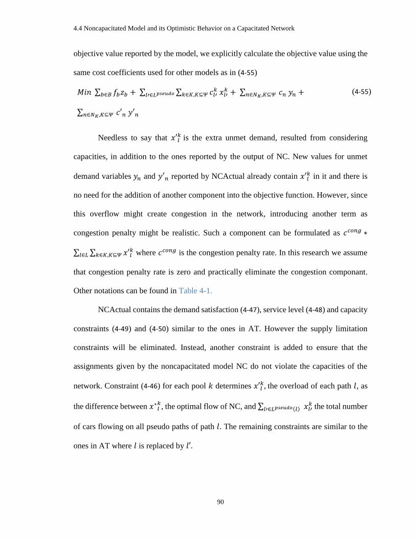
4.4 Noncapacitated Model and its Optimistic Behavior on a Capacitated Network
90
objective value reported by the model, we explicitly calculate the objective value using the
same cost coefficients used for other models as in (4-55)
𝑀𝑖𝑛 ∑ 𝑓𝑏𝑧𝑏𝑏∈𝐵 + ∑ ∑ 𝑐𝑙′𝑘 𝑥𝑙′
𝑘𝑘∈𝐾,𝐾⊆𝛹𝑙′∈𝐿𝑝𝑠𝑒𝑢𝑑𝑜 + ∑ 𝑐𝑛 𝑦𝑛𝑛∈𝑁𝐾,𝐾⊆𝛹 +
∑ 𝑐′𝑛 𝑦′𝑛𝑛∈𝑁𝐾,𝐾⊆𝛹
(4-55)
Needless to say that 𝑥′𝑙𝑘 is the extra unmet demand, resulted from considering
capacities, in addition to the ones reported by the output of NC. New values for unmet
demand variables 𝑦𝑛 and 𝑦′𝑛 reported by NCActual already contain 𝑥′𝑙𝑘 in it and there is
no need for the addition of another component into the objective function. However, since
this overflow might create congestion in the network, introducing another term as
congestion penalty might be realistic. Such a component can be formulated as 𝑐𝑐𝑜𝑛𝑔 ∗
∑ ∑ 𝑥′𝑙𝑘
𝑘∈𝐾,𝐾⊆𝛹𝑙∈𝐿 where 𝑐𝑐𝑜𝑛𝑔 is the congestion penalty rate. In this research we assume
that congestion penalty rate is zero and practically eliminate the congestion componant.
Other notations can be found in Table 4-1.
NCActual contains the demand satisfaction (4-47), service level (4-48) and capacity
constraints (4-49) and (4-50) similar to the ones in AT. However the supply limitation
constraints will be eliminated. Instead, another constraint is added to ensure that the
assignments given by the noncapacitated model NC do not violate the capacities of the
network. Constraint (4-46) for each pool 𝑘 determines 𝑥′𝑙𝑘, the overload of each path 𝑙, as
the difference between 𝑥∗𝑙𝑘, the optimal flow of NC, and ∑ 𝑥𝑙′
𝑘𝑙′∈𝐿𝑝𝑠𝑒𝑢𝑑𝑜(𝑙) the total number
of cars flowing on all pseudo paths of path 𝑙. The remaining constraints are similar to the
ones in AT where 𝑙 is replaced by 𝑙′.

4.5 Trip Planning Algorithm
91
4.5 Trip Planning Algorithm
Both allocation and allocation-timing formulations of the car distribution problem
require an external application to determine the trip plan between the potential supply-
order pairs. We will call such an application a trip planner. In this section, we present a trip
planning model and develop a method to solve it. The objective of such a model is to find
the optimal route for a supply-order pair that minimizes the transportation cost, satisfies
the order expiration date, and respects the physical constraints such as: height clearance
(for railroad segment), weight clearance (for train), and length clearance (for block) as well
as operational constraints such as: the availability of train service, the existence of
dedicated yards for different types of freights, and the availability of yard capacity for
blocking and classification.
Luckily most of the trip planner constraints can be transformed into one of the
following prohibition formulations.
Prohibited arc: certain type of cars might be prohibited from travelling on a certain
arc. For example a tank car might be prohibited from arcs that travel through cities. Arc
prohibition might also happen if the arc's capacity is full. Such a prohibition might be
resolved by simply excluding that arc from the network.
Prohibited maneuver/subpath: sometimes, an arc is not a prohibited arc for the
shipment, but it is prohibited to be selected as the immediate next arc in a path. This kind
of prohibition also happens in road transportation; for example, when a left-turn is
prohibited. Prohibited maneuvers are harder to deal with however they have been studied
recently and efficient algorithms are developed to solve them (Villeneuve and Desaulniers,
4.5 Trip Planning Algorithm
92
2005; Ahmed and Lubiw, 2009; Di Puglia Pugliese and Guerriero, 2011; MAJER, 2011;
Ahmed and Lubiw, 2013).
As mentioned in Section 3.2.2, the service network can be represented as either a
block-train network or a resource constrained blocking network. Next we discuss the trip
planning algorithms for both of these networks.
4.5.1 Trip Planning on the Time-Space Block-Train Network
In addition to the above mentioned physical constraints, another type of constraint
is enforced on the trip planning model as a result of the limitations of the time-space block-
train network.
A path may not originate from an intermediate point of a block. In Figure 3-4 of
Chapter 3 a path can be started by either an inventory arc or an arc with solid circle shape
tail. Once a block starts, it continues until the end of the block (the triangle head). If the
current arc has an open arrow shape head, the next arc in the path must be carrying the
same block and all other arcs are prohibited. Once the car reaches the block destination, it
can travel on an inventory arc or an arc with solid circle shape tail and all other arcs are
prohibited. Hence for a shipment from yard 2 on day 2 to yard 7 on day 6, paths 𝑏5,2: 𝐶2,2 −
𝑏5,2: 𝐶3,3 , 𝑏5,3: 𝐶2,3 − 𝑏5,3: 𝐶3,4 and 𝑏1,2: 𝐴2,2 − 𝑏2,4: 𝐵4,4 are feasible but path 𝑏1,2: 𝐴2,2 −
𝑏6,3: 𝐵4,4 is infeasible. Yard 6 at day 4 is the end of the block 𝑏1,2 (arc head is triangle).
Next arc must be a new block (arc tail must be a solid circle) or an inventory arc (maneuver
from arc 𝑏1,2: 𝐴2,2 to arcs 𝑏4,1: 𝐵4,4 or 𝑏6,3: 𝐵4,4 is prohibited). In fact block 𝑏6,3 is created
on day 3 at yard 5 and is not subject to any intermediate reclassification till its destination
at yard 7 on day 5, and as a result it cannot pickup any cars at yard 6 on day 4.

4.5 Trip Planning Algorithm
93
The trip planning for a shipment between two nodes s and d in a time-space network
can be restated as finding a minimum cost path between s and d while respecting the arc
prohibitions and the maneuver prohibitions. A preliminary and high-level procedure for
finding a trip plan is as follows:
1- Transform the time-space block-train multigragh to simple graph by introducing
virtual nodes
2- Eliminate all prohibited arcs from the network.
3- Find the shortest path between s and d in presence of prohibited maneuvers (e.g. using
the algorithm presented by Villeneuve and Desaulniers (2005)).
4.5.2 Trip Planning on the Time-Space Resource Constrained Blocking Network
Contrary to the block-train network where each arc represents a train segment (and
a block carried on it), arcs in the resource constrained blocking network are blocks and
trains carrying those blocks are listed as block resources. The resource constrained
blocking network is not a multigraph and does not have prohibited maneuvers. Hence after
deleting the prohibited arcs, a shortest path algorithm, such as Dijkstra’s method, can be
used for the trip planning purposes.
1- Eliminate all prohibited arcs from the network.
2- Use Dijkstra's Algorithm to find the shortest path between s and d.
Since trip planning on the resource constrained blocking network is much easier
than on the block-train network, in this research we use this network for trip planning
purposes.

5.1 Allocation-Routing Model
94
Chapter 5
5 Arc-Based Formulation for the Car
Distribution Problem
Contrary to the path-based formulation for the car distribution problem which was
defined on a bipartite multigraph and required a trip planner to provide the arcs of the
graph, practically separating the car routing and car distribution decisions, the arc-based
formulation is defined on a time-space network and integrates car routing and car
distribution decisions in a single Allocation-Routing model. The decision here is not only
supply to demand assignment but also finding the route that the supply will travel from its
origin to destination. As this route is defined on a time-space network, the timing of
movements will be automatically part of the route.
5.1 Allocation-Routing Model
Table 5-1 shows the notation for the indices, sets, parameters and variables used in
the mathematical model. We start our formulation from the objective function. The
objective function (5-1) minimizes the total cost which consists of block setup costs, block
variable costs, delay costs, inventory costs, and unmet demand penalty as well as the contra
costs for customer priorities and preferences (rewards or bonus). Since in the scheduled

5.1 Allocation-Routing Model
95
railroads, general trains are unlikely to be canceled at the operational planning level, train
setup cost is not considered in this model. The details on the components of the cost
function are found in Section 3.2.5.
𝑀𝑖𝑛 ∑ 𝑓𝑏𝑧𝑏𝑏∈𝐵 + ∑ ∑ 𝑐𝑏𝑘 𝑡𝑏
𝑘𝑘∈𝐾,𝐾⊆𝛹𝑏∈𝐵 + ∑ ∑ 𝑐𝑑
𝑑𝑒𝑙𝑎𝑦 𝑡𝑑𝑘
𝑘∈𝐾,𝐾⊆𝛹𝑑∈𝐷 +
∑ ∑ 𝑐𝑖𝑘 𝑡𝑖
𝑘𝑘∈𝐾,𝐾⊆𝛹𝑖∈𝐼 + ∑ 𝑐𝑛 𝑦𝑛𝑛∈𝑁𝐾,𝐾⊆𝛹 + ∑ 𝑐′𝑛 𝑦′𝑛𝑛∈𝑁𝐾,𝐾⊆𝛹 +
∑ ∑ 𝑐𝑛𝑘 𝑥𝑛
𝑘𝑘∈𝐾𝑛𝑛∈𝑁𝐾,𝐾⊆𝛹
(5-1)
First constraint set to consider is the node balance constraints (5-2) in the time-space
flow network. Since substitution is not permitted in this network, each commodity (pool)
has its own balance constraint, resulting in one constraint for each node-pool pair.
∑ 𝑡𝑏𝑘
𝑏∈𝐵𝑚𝑜𝑢𝑡 + ∑ 𝑥𝑛
𝑘𝑛∈𝑁𝑚 ,𝑘∈𝐾𝑛 + 𝑡𝑖=𝐼𝑚𝑜𝑢𝑡
𝑘 +
𝑙𝑚𝑘 − ∑ 𝑡𝑏
𝑘𝑏∈𝐵𝑚
𝑖𝑛 − 𝑡𝑖=𝐼𝑚
𝑖𝑛𝑘 = 𝑠𝑚
𝑘
∀ 𝑚 ∈ 𝑀,∀𝑘 ∈ 𝐾, 𝐾 ⊆ 𝛹
(5-2)
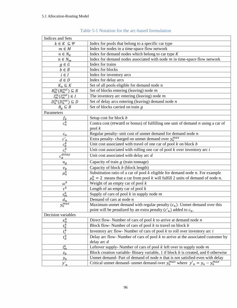
5.1 Allocation-Routing Model
96
Table 5-1 Notation for the arc-based formulation
Indices and Sets
𝑘 ∈ 𝐾 ⊆ 𝛹 Index for pools that belong to a specific car type
𝑚 ∈ 𝑀 Index for nodes in a time-space flow network
𝑛 ∈ 𝑁𝐾 Index for demand nodes which belong to car type 𝐾
𝑛 ∈ 𝑁𝑚 Index for demand nodes associated with node 𝑚 in time-space flow network
𝑔 ∈ 𝐺 Index for trains
𝑏 ∈ 𝐵 Index for blocks
𝑖 ∈ 𝐼 Index for inventory arcs
𝑑 ∈ 𝐷 Index for delay arcs
𝐾𝑛 ⊆ 𝐾 Set of all pools eligible for demand node 𝑛
𝐵𝑚𝑖𝑛(𝐵𝑚
𝑜𝑢𝑡) ⊆ 𝐵 Set of blocks entering (leaving) node 𝑚
𝐼𝑚𝑖𝑛(𝐼𝑚
𝑜𝑢𝑡) ∈ 𝐼 The inventory arc entering (leaving) node 𝑚
𝐷𝑛𝑖𝑛(𝐷𝑛
𝑜𝑢𝑡) ⊆ 𝐷 Set of delay arcs entering (leaving) demand node 𝑛
𝐵𝑔 ⊆ 𝐵 Set of blocks carried on train 𝑔
Parameters
𝑓𝑏 Setup cost for block 𝑏
𝑐𝑛𝑘 Contra cost (reward or bonus) of fulfilling one unit of demand 𝑛 using a car of
pool 𝑘
𝑐𝑛 Regular penalty- unit cost of unmet demand for demand node 𝑛
𝑐′𝑛 Extra penalty- charged on unmet demand over 𝑦𝑛𝑚𝑎𝑥
𝑐𝑏𝑘 Unit cost associated with travel of one car of pool 𝑘 on block 𝑏
𝑐𝑖𝑘 Unit cost associated with rolling one car of pool 𝑘 over inventory arc 𝑖
𝑐𝑑𝑑𝑒𝑙𝑎𝑦
Unit cost associated with delay arc 𝑑
𝑢𝑔 Capacity of train 𝑔 (train tonnage)
𝑣𝑏 Capacity of block 𝑏 (block length)
𝜇𝑛𝑘 Substitution ratio of a car of pool 𝑘 eligible for demand node 𝑛. For example
𝜇𝑛𝑘 = 2 means that a car from pool 𝑘 will fulfill 2 units of demand of node 𝑛.
𝜔𝑘 Weight of an empty car of pool 𝑘
𝜏𝑘 Length of an empty car of pool 𝑘
𝑠𝑚𝑘 Supply of cars of pool 𝑘 in supply node 𝑚
𝑑𝑛 Demand of cars at node 𝑛
𝑦𝑛𝑚𝑎𝑥 Maximum unmet demand with regular penalty (𝑐𝑛). Unmet demand over this
point will be penalized by an extra penalty (𝑐′𝑛) added to 𝑐𝑛.
Decision variables
𝑥𝑛𝑘 Direct flow- Number of cars of pool 𝑘 to arrive at demand node 𝑛
𝑡𝑏𝑘 Block flow- Number of cars of pool 𝑘 to travel on block 𝑏
𝑡𝑖𝑘 Inventory arc flow- Number of cars of pool 𝑘 to roll over inventory arc 𝑖
𝑡𝑑𝑘 Delay arc flow- Number of cars of pool 𝑘 to arrive at the associated customer by
delay arc 𝑑
𝑙𝑚𝑘 Leftover supply- Number of cars of pool 𝑘 left over in supply node 𝑚
𝑧𝑏 Block creation variable- Binary variable, 1 if block 𝑏 is created, and 0 otherwise
𝑦𝑛 Unmet demand- Part of demand of node 𝑛 that is not satisfied even with delay
𝑦′𝑛 Critical unmet demand- unmet demand over 𝑦𝑛𝑚𝑎𝑥 where 𝑦′𝑛 = 𝑦𝑛 − 𝑦𝑛
𝑚𝑎𝑥
5.1 Allocation-Routing Model
97
Balance constraints for demand nodes are formulated as (5-3). Since contrary to the
time-space network nodes substitution is permitted at customer level, balance constraints
here are not defined for node-pool pairs and there exists only one constraint for each
demand node. Constraint (5-4) is the soft constraint on the maximum permitted unmet
demand and defines the critical unmet demand (subject to extra penalty).
∑ (𝑥𝑛𝑘 + ∑ 𝜇𝑛
𝑘𝑡𝑑𝑘
𝑑∈𝐷𝑛𝑖𝑛 )𝑘∈𝐾𝑛 + 𝑦𝑛 −
∑ ∑ 𝜇𝑛𝑘𝑡𝑑𝑘
𝑑∈𝐷𝑛𝑜𝑢𝑡𝑘∈𝐾𝑛 = 𝑑𝑛
∀ 𝑛 ∈ 𝑁𝐾, 𝐾 ⊆ 𝛹 (5-3)
𝑦′𝑛 ≥ 𝑦𝑛 − 𝑦𝑛𝑚𝑎𝑥 ∀ 𝑛 ∈ 𝑁𝐾, 𝐾 ⊆ 𝛹 (5-4)
After formulating the node balance constraints, the network capacity constraints are
formulated for both trains and blocks as shown in (5-5) and (5-6) respectively.
∑ ∑ 𝜔𝑘𝑡𝑏𝑘
𝑘∈𝐾,𝐾⊆𝛹𝑏∈𝐵𝑔 ≤ 𝑢𝑔 ∀𝑔 ∈ 𝐺 (5-5)
∑ 𝜏𝑘𝑡𝑏𝑘
𝑘∈𝐾,𝐾⊆𝛹 ≤ 𝑣𝑏𝑧𝑏 ∀ 𝑏 ∈ 𝐵 (5-6)
Constraint sets (5-2) to (5-6) along with the binary constraint associated with the
block creations and non-negativity and integrality constraints for all other decision
variables will guarantee the supply availability, demand satisfaction and network
capacities; however they fail with respect to the order expiration dates.
Figure 5-1 shows five demand nodes associated with a single customer profile in
five different days with a maximum accepted delay of two days for each order-day. Each
node hosts the inflow of two backward arrows, associated with the flow that arrives by one
day delay and two-day delay. The reason we introduce two arcs, rather than only one arc,
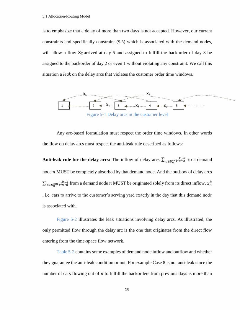
5.1 Allocation-Routing Model
98
is to emphasize that a delay of more than two days is not accepted. However, our current
constraints and specifically constraint (5-3) which is associated with the demand nodes,
will allow a flow X2 arrived at day 5 and assigned to fulfill the backorder of day 3 be
assigned to the backorder of day 2 or even 1 without violating any constraint. We call this
situation a leak on the delay arcs that violates the customer order time windows.
Figure 5-1 Delay arcs in the customer level
Any arc-based formulation must respect the order time windows. In other words
the flow on delay arcs must respect the anti-leak rule described as follows:
Anti-leak rule for the delay arcs: The inflow of delay arcs ∑ 𝜇𝑛𝑘𝑡𝑑𝑘
𝑑∈𝐷𝑛𝑖𝑛 to a demand
node 𝑛 MUST be completely absorbed by that demand node. And the outflow of delay arcs
∑ 𝜇𝑛𝑘𝑡𝑑𝑘
𝑑∈𝐷𝑛𝑜𝑢𝑡 from a demand node 𝑛 MUST be originated solely from its direct inflow, 𝑥𝑛
𝑘
, i.e. cars to arrive to the customer’s serving yard exactly in the day that this demand node
is associated with.
Figure 5-2 illustrates the leak situations involving delay arcs. As illustrated, the
only permitted flow through the delay arc is the one that originates from the direct flow
entering from the time-space flow network.
Table 5-2 contains some examples of demand node inflow and outflow and whether
they guarantee the anti-leak condition or not. For example Case 8 is not anti-leak since the
number of cars flowing out of 𝑛 to fulfill the backorders from previous days is more than
5 4 3 2 1 X3
X2 X5
X1
X4

5.1 Allocation-Routing Model
99
the direct flow to 𝑛. This means part of this backorder flow is coming either from the unmet
demand, a total nonsense acquisition!, or from the inflow of delay arcs which is a clear
violation of anti-leak rule. Similarly case 9 is violating anti-leak rule since its delay arcs’
inflow is more than its demand and based on demand node balance constraint, the extra
units will flow through delay arcs flowing out of 𝑛, a leak situation by definition.
Figure 5-2 Permitted flow vs leak in customer level
Table 5-2 Permitted flows vs leak in the customer level
Case
# 𝒅𝒏 ∑ 𝝁𝒏
𝒌𝒕𝒅𝒌
𝒅∈𝑫𝒏𝒊𝒏
𝒙𝒏𝒌 𝒚𝒏 ∑ 𝝁𝒏
𝒌𝒕𝒅𝒌
𝒅∈𝑫𝒏𝒐𝒖𝒕
Extra
condition
Anti-
leak?
1 10 3 3 4 0 YES
2 𝑑𝑛 0 ≤ 𝑎 ≤ 𝑑𝑛 0 ≤ 𝑏 ≤ 𝑑𝑛 0 ≤ 𝑐 ≤ 𝑑𝑛 0 𝑎 + 𝑏 + 𝑐= 𝑑𝑛
YES
3 10 0 5 8 3 YES
4 𝑑𝑛 0 0 ≤ 𝑏 0 ≤ 𝑐 ≤ 𝑑𝑛 0 ≤ 𝑑 ≤ 𝑑𝑛 𝑏 + 𝑐 − 𝑑= 𝑑𝑛
YES
5 10 5 5 5 5 YES?
6 𝑑𝑛 0 ≤ 𝑎 0 ≤ 𝑏 0 ≤ 𝑐 ≤ 𝑑𝑛 𝑑 ≤ 𝑎 𝑎 + 𝑏 + 𝑐− 𝑑 = 𝑑𝑛
YES?
7 10 4 5 7 6 NO
8 𝑑𝑛 0 < 𝑏 𝑑 > 𝑏 NO
9 𝑑𝑛 𝑑𝑛 < 𝑎 NO
10 0 0 0 < 𝑎 0 0 < 𝑎 YES
m
𝑛, 𝑑𝑛
𝑥𝑛𝑘
∑ 𝜇𝑛𝑘𝑡𝑑𝑘
𝑑∈𝐷𝑛𝑖𝑛
∑ 𝜇𝑛𝑘𝑡𝑑𝑘
𝑑∈𝐷𝑛𝑜𝑢𝑡
𝑦𝑛
!Leak!
!Leak!
Permitted

5.2 Formulating the Anti-Leak Rule using Extra Constraints
100
5.2 Formulating the Anti-Leak Rule using Extra Constraints
In order to formulate the anti-leak rule we introduced two extra constraints.
Constraint (5-7) states that for each demand node, the total backorder and unmet demand
should not be more than its demand. Constraint (5-8) states that total number of cars of pool
𝑘 carried back from node 𝑛 (associated to a specific customer in a specific day) to fulfill
the backorder of previous days of the same customer cannot be more than the number of
cars of the same pool that has entered 𝑛 directly from the time-space flow network.
∑ ∑ 𝜇𝑛𝑘𝑡𝑑𝑘
𝑑∈𝐷𝑛𝑖𝑛𝑘∈𝐾𝑛 + 𝑦𝑛 ≤ 𝑑𝑛 ∀ 𝑛 ∈ 𝑁𝐾, ∀ 𝐾 ⊆ 𝛹 (5-7)
∑ 𝜇𝑛𝑘𝑡𝑑𝑘
𝑑∈𝐷𝑛𝑜𝑢𝑡 ≤ 𝑥𝑛
𝑘 ∀ 𝑛 ∈ 𝑁𝐾, ∀ 𝐾 ⊆ 𝛹, 𝑘 ∈ 𝐾𝑛 (5-8)
We were hoping that these two constraints will guarantee the anti-leak rule for the
delay arcs. However numerical results showed that these constraints are not sufficient to
guarantee this rule. Furthermore it turned out that (5-7) is redundant in presence of (5-3)
and (5-8). Instead of insisting on introducing new set of constraints to formulate the anti-
leak condition, we decided to change our decision variables in such a way that this
condition is satisfied. Developing such constraint set however could be a good theoretical
work and is an area open to the researchers.
5.3 Formulating the Anti-Leak Rule with Redefining the Decision
Variables
In order to guarantee anti-leak condition among delay arcs, as illustrated in Figure
5-3, we split the flow of cars arriving at demand node 𝑛, i.e. 𝑥𝑛𝑘, to two separate variables:
one variable to represent the part of this flow that fulfills its own demand, and will liberally

5.3 Formulating the Anti-Leak Rule with Redefining the Decision Variables
101
note it by 𝑥𝑛𝑘, and another variable to represent the part of the flow that will cover the
backorder of the same customer from previous days, and will denote it by 𝑥′𝑛𝑘 , where 𝑥′𝑛
𝑘 =
∑ 𝑡𝑑𝑘
𝑑∈𝐷𝑛𝑜𝑢𝑡 .
Figure 5-3 Dealing with delay arc flow using a new variable
This change affects objective function (5-1), node balance constraint (5-2) and
demand node balance constraint (5-3) and transforms them to (5-9), (5-10), and (5-11),
respectively.
𝑀𝑖𝑛 ∑ 𝑓𝑏𝑧𝑏𝑏∈𝐵 + ∑ ∑ 𝑐𝑏𝑘 𝑡𝑏
𝑘𝑘∈𝐾,𝐾⊆𝛹𝑏∈𝐵 + ∑ ∑ 𝑐𝑑
𝑘 𝑡𝑑𝑘
𝑘∈𝐾,𝐾⊆𝛹𝑑∈𝐷 +
∑ ∑ 𝑐𝑖𝑘 𝑡𝑖
𝑘𝑘∈𝐾,𝐾⊆𝛹𝑖∈𝐼 + ∑ 𝑐𝑛 𝑦𝑛𝑛∈𝑁𝐾,𝐾⊆𝛹 + ∑ 𝑐′𝑛 𝑦′𝑛𝑛∈𝑁𝐾,𝐾⊆𝛹 +
∑ ∑ 𝑐𝑛𝑘 (𝑥𝑛
𝑘 + 𝑥′𝑛𝑘)𝑘∈𝐾𝑛𝑛∈𝑁𝐾,𝐾⊆𝛹
(5-9)
∑ 𝑡𝑏𝑘
𝑏∈𝐵𝑚𝑜𝑢𝑡 + ∑ (𝑥𝑛
𝑘 + 𝑥′𝑛𝑘)𝑛∈𝑁𝑚 𝑤ℎ𝑒𝑟𝑒 𝑘∈𝐾𝑛 +
𝑡𝑖=𝐼𝑚𝑜𝑢𝑡𝑘 + 𝑙𝑚
𝑘 − ∑ 𝑡𝑏𝑘
𝑏∈𝐵𝑚𝑖𝑛 − 𝑡
𝑖=𝐼𝑚𝑖𝑛
𝑘 = 𝑠𝑚𝑘
∀ 𝑚 ∈ 𝑀,∀𝑘 ∈ 𝐾, ∀ 𝐾 ⊆
𝛹
(5-10)
m
n, dn
𝑥𝑛𝑘
∑ 𝜇𝑛𝑘𝑡𝑑𝑘
𝑑∈𝐷𝑛𝑖𝑛
∑ 𝜇𝑛𝑘𝑡𝑑𝑘
𝑑∈𝐷𝑛𝑜𝑢𝑡
= 𝑥′𝑛𝑘
𝑦𝑛
𝑥′𝑛𝑘

5.3 Formulating the Anti-Leak Rule with Redefining the Decision Variables
102
∑ (𝑥𝑛𝑘 + 𝑥′𝑛
𝑘 + ∑ 𝜇𝑛𝑘𝑡𝑑𝑘
𝑑∈𝐷𝑛𝑖𝑛 )𝑘∈𝐾𝑛 + 𝑦𝑛 −
∑ ∑ 𝜇𝑛𝑘𝑡𝑑𝑘
𝑑∈𝐷𝑛𝑜𝑢𝑡𝑘∈𝐾𝑛 = 𝑑𝑛
∀ 𝑛 ∈ 𝑁𝐾, ∀ 𝐾 ⊆ 𝛹 (5-11)
and adds following two constraints to the model as well.
∑ 𝑡𝑑𝑘
𝑑∈𝐷𝑛𝑜𝑢𝑡 = 𝑥′𝑛
𝑘 ∀ 𝑛 ∈ 𝑁𝐾, ∀ 𝐾 ⊆ 𝛹, 𝑘 ∈ 𝐾𝑛 (5-12)
𝑥′𝑛𝑘 ≥ 0 𝑎𝑛𝑑 𝑖𝑛𝑡𝑒𝑔𝑒𝑟 ∀ 𝑛 ∈ 𝑁𝐾, ∀ 𝐾 ⊆ 𝛹, 𝑘 ∈ 𝐾𝑛 (5-13)
The arc-based formulation of the car distribution problem is as follows:
𝑀𝑖𝑛 ∑ 𝑓𝑏𝑧𝑏𝑏∈𝐵 + ∑ ∑ 𝑐𝑏𝑘 𝑡𝑏
𝑘𝑘∈𝐾,𝐾⊆𝛹𝑏∈𝐵 + ∑ ∑ 𝑐𝑑
𝑘 𝑡𝑑𝑘
𝑘∈𝐾,𝐾⊆𝛹𝑑∈𝐷 +
∑ ∑ 𝑐𝑖𝑘 𝑡𝑖
𝑘𝑘∈𝐾,𝐾⊆𝛹𝑖∈𝐼 + ∑ 𝑐𝑛 𝑦𝑛𝑛∈𝑁𝐾,𝐾⊆𝛹 + ∑ 𝑐′𝑛 𝑦′𝑛𝑛∈𝑁𝐾,𝐾⊆𝛹 +
∑ ∑ 𝑐𝑛𝑘 (𝑥𝑛
𝑘 + 𝑥′𝑛𝑘)𝑘∈𝐾𝑛𝑛∈𝑁𝐾,𝐾⊆𝛹
(5-14)
∑ 𝑡𝑏𝑘
𝑏∈𝐵𝑚𝑜𝑢𝑡 + ∑ (𝑥𝑛
𝑘 + 𝑥′𝑛𝑘)𝑛∈𝑁𝑚 𝑤ℎ𝑒𝑟𝑒 𝑘∈𝐾𝑛 +
𝑡𝑖=𝐼𝑚𝑜𝑢𝑡𝑘 + 𝑙𝑚
𝑘 − ∑ 𝑡𝑏𝑘
𝑏∈𝐵𝑚𝑖𝑛 − 𝑡
𝑖=𝐼𝑚𝑖𝑛
𝑘 = 𝑠𝑚𝑘
∀ 𝑚 ∈ 𝑀,∀𝑘 ∈ 𝐾, ∀ 𝐾 ⊆
𝛹
(5-15)
∑ (𝑥𝑛𝑘 + 𝑥′𝑛
𝑘 + ∑ 𝜇𝑛𝑘𝑡𝑑𝑘
𝑑∈𝐷𝑛𝑖𝑛 )𝑘∈𝐾𝑛 + 𝑦𝑛 −
∑ ∑ 𝜇𝑛𝑘𝑡𝑑𝑘
𝑑∈𝐷𝑛𝑜𝑢𝑡𝑘∈𝐾𝑛 = 𝑑𝑛
∀ 𝑛 ∈ 𝑁𝐾, ∀ 𝐾 ⊆ 𝛹 (5-16)
𝑦′𝑛 ≥ 𝑦𝑛 − 𝑦𝑛𝑚𝑎𝑥 ∀ 𝑛 ∈ 𝑁𝐾, ∀ 𝐾 ⊆ 𝛹 (5-17)
∑ 𝑡𝑑𝑘
𝑑∈𝐷𝑛𝑜𝑢𝑡 = 𝑥′𝑛
𝑘 ∀ 𝑛 ∈ 𝑁𝐾, ∀ 𝐾 ⊆ 𝛹, 𝑘 ∈ 𝐾𝑛 (5-18)
∑ ∑ 𝜔𝑘𝑡𝑏𝑘
𝑘∈𝐾,𝐾⊆𝛹𝑏∈𝐵𝑔 ≤ 𝑢𝑔 ∀𝑔 ∈ 𝐺 (5-19)
∑ 𝜏𝑘𝑡𝑏𝑘
𝑘∈𝐾,𝐾⊆𝛹 ≤ 𝑣𝑏𝑧𝑏 ∀ 𝑏 ∈ 𝐵 (5-20)

5.3 Formulating the Anti-Leak Rule with Redefining the Decision Variables
103
𝑡𝑗𝑘 ≥ 0 𝑎𝑛𝑑 𝑖𝑛𝑡𝑒𝑔𝑒𝑟 ∀𝑗 ∈ 𝐸 = 𝐵|𝐼|𝐷, ∀𝑘 ∈
𝐾,𝐾 ⊆ 𝛹
(5-21)
𝑥𝑛𝑘 , 𝑥′𝑛
𝑘 ≥ 0 𝑎𝑛𝑑 𝑖𝑛𝑡𝑒𝑔𝑒𝑟 ∀ 𝑛 ∈ 𝑁𝐾, ∀ 𝐾 ⊆ 𝛹, 𝑘 ∈ 𝐾𝑛 (5-22)
𝑦𝑛, 𝑦′𝑛 ≥ 0 ∀ 𝑛 ∈ 𝑁𝐾, ∀ 𝐾 ⊆ 𝛹 (5-23)
𝑧𝑏 ∈ {0,1} ∀𝑏 ∈ 𝐵 (5-24)
Furthermore we can see, easily, that constraints (5-11) and (5-12) are only defining
the unmet demand (𝑦𝑛) and backordered demand (𝑥′𝑛𝑘), respectively. In other words we
can simultaneously decrease the number of constraints and variables by replacing 𝑦𝑛 by its
equivalent term 𝑑𝑛 − ∑ (𝜇𝑛𝑘𝑥𝑛
𝑘 + ∑ 𝜇𝑛𝑘𝑡𝑑𝑘
𝑑∈𝐷𝑛𝑖𝑛 )𝑘∈𝐾𝑛 and by replacing 𝑥′𝑛
𝑘 by ∑ 𝑡𝑑𝑘
𝑑∈𝐷𝑛𝑜𝑢𝑡 .
The non-negativity and integrality constraint (5-13) is automatically satisfied since 𝑡𝑑𝑘 ≥
0 𝑎𝑛𝑑 𝑖𝑛𝑡𝑒𝑔𝑒𝑟 ∀𝑑 ∈ 𝐷, 𝑘 ∈ 𝐾,𝐾 ⊆ 𝛹; however 𝑦𝑛 ≥ 0 is not guaranteed and should be
added explicitly as a constraint, i.e. ∑ (𝜇𝑛𝑘𝑥𝑛
𝑘 + ∑ 𝜇𝑛𝑘𝑡𝑑𝑘
𝑑∈𝐷𝑛𝑖𝑛 )𝑘∈𝐾𝑛 ≤ 𝑑𝑛.
Finally the ∑ ∑ 𝑐𝑑𝑘 𝑡𝑑
𝑘𝑘∈𝐾,𝐾⊆𝛹𝑑∈𝐷 component in the objective function can be
replaced by its equivalent term ∑ ∑ ∑ 𝑐𝑑𝑘 𝑡𝑑
𝑘𝑘∈𝐾𝑛𝑑∈𝐷𝑛
𝑖𝑛𝑛∈𝑁𝐾,𝐾⊆𝛹 . The arc-based formulation
of the multicommodity car distribution problem, after aggregating the coefficients, is as
follows:
Allocation-Routing (AR)
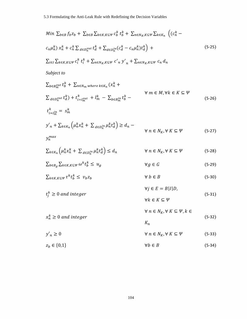
5.3 Formulating the Anti-Leak Rule with Redefining the Decision Variables
104
𝑀𝑖𝑛 ∑ 𝑓𝑏𝑧𝑏𝑏∈𝐵 + ∑ ∑ 𝑐𝑏𝑘 𝑡𝑏
𝑘𝑘∈𝐾,𝐾⊆𝛹𝑏∈𝐵 + ∑ ∑ 𝑘∈𝐾𝑛𝑛∈𝑁𝐾,𝐾⊆𝛹 ((𝑐𝑛
𝑘 −
𝑐𝑛𝜇𝑛𝑘) 𝑥𝑛
𝑘 + 𝑐𝑛𝑘 ∑ 𝑡𝑑
𝑘 𝑑∈𝐷𝑛
𝑜𝑢𝑡 + ∑ (𝑐𝑑𝑘 − 𝑐𝑛𝜇𝑛
𝑘)𝑡𝑑𝑘
𝑑∈𝐷𝑛𝑖𝑛 ) +
∑ ∑ 𝑐𝑖𝑘 𝑡𝑖
𝑘𝑘∈𝐾,𝐾⊆𝛹𝑖∈𝐼 + ∑ 𝑐′𝑛 𝑦
′𝑛𝑛∈𝑁𝐾,𝐾⊆𝛹 + ∑ 𝑐𝑛𝑛∈𝑁𝐾,𝐾⊆𝛹 𝑑𝑛
(5-25)
Subject to
∑ 𝑡𝑏𝑘
𝑏∈𝐵𝑚𝑜𝑢𝑡 + ∑ (𝑥𝑛
𝑘 +𝑛∈𝑁𝑚 𝑤ℎ𝑒𝑟𝑒 𝑘∈𝐾𝑛
∑ 𝑡𝑑𝑘
𝑑∈𝐷𝑛𝑜𝑢𝑡 ) + 𝑡𝑖=𝐼𝑚𝑜𝑢𝑡
𝑘 + 𝑙𝑚𝑘 − ∑ 𝑡𝑏
𝑘𝑏∈𝐵𝑚
𝑖𝑛 −
𝑡𝑖=𝐼𝑚
𝑖𝑛𝑘 = 𝑠𝑚
𝑘
∀ 𝑚 ∈ 𝑀,∀𝑘 ∈ 𝐾 ⊆ 𝛹
(5-26)
𝑦′𝑛 + ∑ (𝜇𝑛𝑘𝑥𝑛
𝑘 + ∑ 𝜇𝑛𝑘𝑡𝑑𝑘
𝑑∈𝐷𝑛𝑖𝑛 )𝑘∈𝐾𝑛 ≥ 𝑑𝑛 −
𝑦𝑛𝑚𝑎𝑥
∀ 𝑛 ∈ 𝑁𝐾, ∀ 𝐾 ⊆ 𝛹 (5-27)
∑ (𝜇𝑛𝑘𝑥𝑛
𝑘 + ∑ 𝜇𝑛𝑘𝑡𝑑𝑘
𝑑∈𝐷𝑛𝑖𝑛 )𝑘∈𝐾𝑛 ≤ 𝑑𝑛 ∀ 𝑛 ∈ 𝑁𝐾, ∀ 𝐾 ⊆ 𝛹 (5-28)
∑ ∑ 𝜔𝑘𝑡𝑏𝑘
𝑘∈𝐾,𝐾⊆𝛹𝑏∈𝐵𝑔 ≤ 𝑢𝑔 ∀𝑔 ∈ 𝐺 (5-29)
∑ 𝜏𝑘𝑡𝑏𝑘
𝑘∈𝐾,𝐾⊆𝛹 ≤ 𝑣𝑏𝑧𝑏 ∀ 𝑏 ∈ 𝐵 (5-30)
𝑡𝑗𝑘 ≥ 0 𝑎𝑛𝑑 𝑖𝑛𝑡𝑒𝑔𝑒𝑟
∀𝑗 ∈ 𝐸 = 𝐵|𝐼|𝐷,
∀𝑘 ∈ 𝐾 ⊆ 𝛹
(5-31)
𝑥𝑛𝑘 ≥ 0 𝑎𝑛𝑑 𝑖𝑛𝑡𝑒𝑔𝑒𝑟
∀ 𝑛 ∈ 𝑁𝐾, ∀ 𝐾 ⊆ 𝛹, 𝑘 ∈
𝐾𝑛
(5-32)
𝑦′𝑛 ≥ 0 ∀ 𝑛 ∈ 𝑁𝐾, ∀ 𝐾 ⊆ 𝛹 (5-33)
𝑧𝑏 ∈ {0,1} ∀𝑏 ∈ 𝐵 (5-34)
5.3 Formulating the Anti-Leak Rule with Redefining the Decision Variables
105
Chapter 6
6 Numerical Results
In this Chapter we evaluate the validity of the models presented in this Dissertation
as well as the efficiency of the solution methods developed to solve them. The car
distribution models are implemented in Java and CPLEX solver is called using Concert
Technology. We could have used CPLEX Optimization Programming Language (OPL)
instead, but the Java programming provided us the opportunity to have trip planning,
pseudo path generation and car distribution models, as well as the random case example
generator all in one place, without the need to switch between different software.
Furthermore, integrating a java program into the ERP system, compared to a stand-alone
software, is easier for the railroad IT departments since Java, compared to OPL, is more
popular in the industry. Before proceeding we should define some keywords that we will
use in this chapter extensively.
Factors set A: is a set of parameters that are used to generate the input sets of the models
(e.g. factor set A = (networkName, numCarTypes, numDemandProfiles,
numSupplyNodes, capacityFactor) ).

5.3 Formulating the Anti-Leak Rule with Redefining the Decision Variables
106
Problem size B of factors set A: a problem size is an instance of factors set (e.g. problem
size B= (Small, 2, 2, 3, 1) means a problem which is defined on top of a network called
Small, has 2 car types, 2 demand profiles and 3 supply nodes and the network capacities
are equal to the ones in the Small network (multiplied by 1) ).
Case example/ instance C (of size B): a data set that contains the coefficients of the car
distribution model or the information that can be used to generate those coefficients. (e.g.
Case examples C1 = (Small, {carType1, carType2}, {Profile1, Profile2}, {node1, node2,
node5}, 1) and C2 = (Small, {carType1, carType2}, {Profile3, Profile8}, {node3, node5,
node8}, 1) both are from the problem size of B = (Small, 2, 2, 3, 1) of Factor set A =
(networkName, numCarTypes, numDemandProfiles, numSupplyNodes, capacityFactor))
Scenario D (on Case example C): a relation that takes a case example C, and an element
of Factor set A as input and generates multiple case scenarios. (e.g. f(C2, capacityFactor)
= { C21, C22} where the only difference between C21 = (Small, {carType1, carType2},
{Profile3, Profile8}, {node3, node5, node8}, 2) and C22 = (Small, {carType1, carType2},
{Profile3, Profile8}, {node3, node5, node8}, 6) is that the capacities of blocks and trains
in C22 are triple of the capacities of the same blocks and trains in C21.
We continue this chapter with some techniques that we used to verify the accuracy
of the computer programs and the validity of the models and solution techniques. Then we
illustrate those models in a small numerical example and finally evaluate the performance
of different solution methods and heuristics on large scale problems.

6.1 Verification and Validation
107
6.1 Verification and Validation
Car distribution planning is an operational decision frequently made by the railroad
companies. The frequency of the decisions might change from one to several times per day.
Besides the impact on the railroad costs and revenues, the car distribution planning decision
affects multiple stakeholders inside and outside the industry. Each decision made at each
time by the car distribution department affects their own future decisions because of the
direct impact on the supply and demand. The work load of employees working at the
classification yards is also affected by these decisions. The customer's operations are highly
influenced by the railroad decisions and a plant might be temporally shut down as a result
of car supply shortage. A poor car distribution model might develop unstable outputs and
consequently result in the loss of customer goodwill. This is why the car distribution model
needs to be verified and validated as part of its development process. Based on AIAA
(1998), validation is defined as the process of determining the degree at which a model is
an accurate representation of the real world from the perspective of the intended uses of
the model. Verification is defined as the process of determining that a model
implementation accurately represents the developer’s conceptual description of the model
and the solution to the model.
Roughly speaking, validation can be expressed by the query "Are you building the
right thing?" and verification by "Are you building it right?". We followed some steps to
ensure that we have proposed the right models and solution methods and have implemented
them correctly.

6.1 Verification and Validation
108
The conceptual model was presented in the INFORMS 2014 conference and was
further discussed by the railroad experts to ensure that it represents the real world problem
and hence is useful for the practitioners in the industry.
After validating the conceptual model, the mathematical model as well as the
proposed solution methods were discussed and validated by the PhD Dissertation
Committee members.
A computer program was developed in Java; and its accuracy was verified using
debugging techniques, observational verification and analytical verification. For
debugging we made sure the computer program is free of any compile or run time error.
However debugging is not enough to make sure the computer program represents the
mathematical model. In this research we used two sets of techniques to verify that the
computer program reflects the mathematical model. First for a number of small size
problems we explicitly compared the mathematical model generated by the computer
program with the mathematical model written based on the proposed formulation. We
called this technique an observational verification. Observational verification was
powerful enough to enable us to fix some basic errors like typo of “+” instead of “-“ or “=”
instead of “>=”, etc. However, because of the small and simple nature of those case
examples, it is not sufficient to completely verify the accuracy of the program. Writing the
mathematical model for the larger size and more complex case examples to compare with
the exported model from the computer program is not practical, because of huge number
of constraints and variables. In order to verify the accuracy of models for the larger size
problems we used analytical verification techniques. Besides the popular techniques such
as extreme condition tests, etc. we developed another analytical technique as a set of rules
6.1 Verification and Validation
109
that must always hold based on the nature of the models presented in this research. The
models are abbreviated as follows:
PA is the path based Pure Allocation model, AT is the path based Allocation Timing
model, NC is the Noncapacitated path based model, and AR is the arc based Allocation-
Routing model.
Property 6-1 Superset-Subset Relations: The objective values associated with the optimal
solutions of different models presented in this Dissertation, on a given case example (set
of inputs), satisfy the following relations:
a- AT <= PA
b- AR <= AT, PA
c- NC <= PA, AT, AR
d- AR (after relaxing capacities) = NC
where the model abbreviations represent the respective model objective values.
Prof: Property 6-1a always holds since the feasible region of AT is a superset of feasible
region of PA. This comes from this fact that the set of pseudo paths of a trip plan generated
by Pseudo Path Generator presented in Section 4.3.1 always contains the trip plan itself.
For proving Property 6-1b, it is sufficient to prove that AR <= AT since AT <= PA holds
based on Property 6-1a. AR <= AT always holds since the allocation and routing decisions
are integrated in one model in AR while AT only deals with the allocation decision while
routing decision is made by Trip Planner. The optimal solutions of integrated models are
known to be better than the aggregated models.
Next we prove Property 6-1c in three steps: i) NC <= PA always holds since the path
connecting a given supply-demand pair in NC is the same as the path connecting the same

6.1 Verification and Validation
110
pair in PA with the only difference that this path is capacitated in PA. ii) NC <= AT also
holds true since although a given supply-order pair might be connected with more than one
paths in AT, NC uses the shortest path among them without any capacity limits. iii) NC <=
AR also always holds. Although AR integrates the car routing and allocation decisions and
based on Property 6-1b always overperforms PA and AT, the comparison with NC model
is different. If we convert the arc flow decisions made by AR to path flows from supply to
demand, the best path that can be offered by AR, for a given supply-demand pair is the
shortest path between them. However in the presence of capacities, in the optimal solution
of AR, a supply-demand pair might not be necessarily connected using this best path. On
the other hand NC always uses the shortest path for each given supply-demand pair. Hence
from i, ii, and iii we conclude that Property 6-1c always holds.
Property 6-1d always holds since if capacity limits are relaxed, for a given supply-demand
pair, the integrated car routing and allocation model AR, after transforming the arc flows
to path flows, will pick the shortest path to connect them. Hence the arc based formulation
of AR model after relaxing capacity limits is equivalent to the path based noncapacitated
model NC. ■
Table 6-1 introduces four networks that are used in this chapter to verify and
validate the models and their solution procedures. The first static network has only 5 yards,
6 blocks, 3 trains and 9 train segments, resulting in a time-space network of 45 nodes, 18
blocks, 9 train and 27 train segments in a 3-day time horizon. Because of its small size we
called this network “Super Tiny Network”. The Super Tiny Network was used for
observational verification.

6.1 Verification and Validation
111
The second network is called “Tiny Network” and has the same yards, blocks and
trains but in an 18-day time horizon. Tiny Network is too large to be used for observational
verification and was used for fast analytical verification only. All models were run for
hundreds of times on randomly generated case examples on top of the Tiny Network.
Anytime any of the rules in Property 6-1 were violated the execution was terminated and
the cause of violation was investigated. For example, the output of one model was fed to
another model by stablishing those variables to the values in the other model and if the new
formulation was infeasible the causes of infeasibility were investigated. CPLEX solver in
interactive mode was extremely helpful in finding the conflicts among the constraints.
The size of Tiny Network was big enough to capture some of the issues in the
computer programs and small enough to be able to generate and run a case example in a
few seconds. However the final verification was performed on a network with larger size
called “Medium Network”. This network has 78 yards, 239 blocks, 95 trains and 323 train
segments. The datasets for the physical and blocking networks were acquired from the
2011 - RAS Problem Solving Competition in train design (https://www.informs.org/
Community/RAS/Problem-Solving-Competition/2011-RAS-Problem-Solving-
Competition). The train design data including the train routing and train makeup plans were
generously provided by one of the award winners, Team OR at UNIMI. Execution of all
models for more than 10000 times on case examples of different scales generated on top
of the Medium Network, verified the accuracy of all formulations based on the analytical
verification techniques. We also used the same network for the illustrative example that
will be presented in Section 6.2.

6.1 Verification and Validation
112
After verifying that the computer program correctly represents the model, the next
step was to validate the performance of different models, especially our path based
Allocation-Timing model, by benchmarking them against each other and also against the
noncapacitated model as the current practice of many railway industries. Case examples
used for validation purposes were generated on a bigger network called “Large Network”
with 440 yards, 1369 blocks, 624 trains and 2167 train segments which in an 18-day time
horizon results in 34941 nodes, 24642 blocks, 11232 trains and 39005 train segments. The
Large Network was created by duplicating and manipulating the Medium Network for 4
times and another medium size network available at RAS 2011 competition for 2 times and
connecting them in such a way that all components of physical, block and train networks
stay connected.
As part of the validation phase, four performance measures were defined: a)
objective value and b) fulfillment ratio as measures of efficiency of the models, and c) run
time and d) relative optimality gap, as measures of efficiency of the solution methods. For
each model, the objective value is the value of the objective function in the optimal
solution, or the best incumbent if the optimum is not met; the fulfillment ratio is the ratio
of satisfied demand to the entire demand for all car types and all customers; run time is the
CPU time for solving the problem; and the relative optimality gap is a gauge to measure
the gap between the current incumbent and tightest known bound and is identical to EpGap
in CPLEX solver which is calculated by (6-1):
𝐸𝑝𝐺𝑎𝑝 =|𝑓(𝑏𝑒𝑠𝑡 𝑛𝑜𝑑𝑒) − 𝑓(𝑏𝑒𝑠𝑡 𝑖𝑛𝑡𝑒𝑔𝑒𝑟 𝑠𝑜𝑙𝑢𝑡𝑖𝑜𝑛)|
1𝑒 − 10 + |𝑓(𝑏𝑒𝑠𝑡 𝑖𝑛𝑡𝑒𝑔𝑒𝑟 𝑠𝑜𝑙𝑢𝑡𝑖𝑜𝑛)|=
|𝐿𝐵 − 𝑈𝐵|
1𝑒 − 10 + |𝑈𝐵|
(6-1)
The results of the validation phase are presented in Section 6.3.
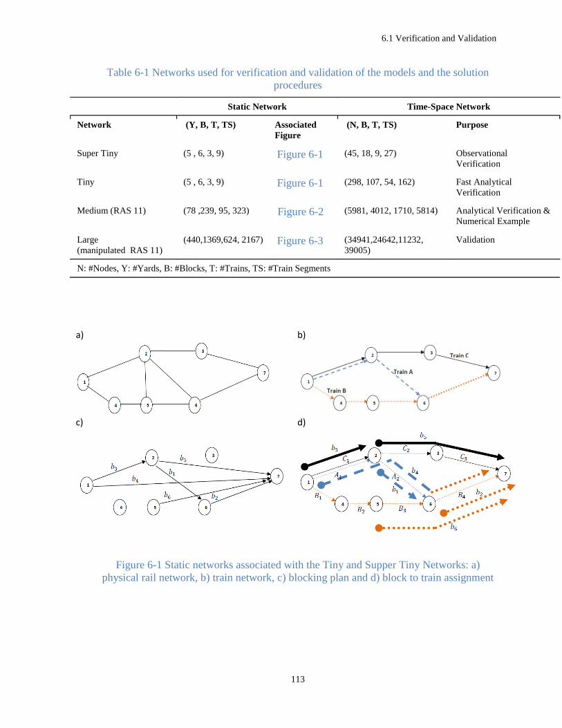
6.1 Verification and Validation
113
Table 6-1 Networks used for verification and validation of the models and the solution
procedures
Static Network Time-Space Network
Network (Y, B, T, TS) Associated
Figure
(N, B, T, TS) Purpose
Super Tiny (5 , 6, 3, 9) Figure 6-1 (45, 18, 9, 27) Observational
Verification
Tiny (5 , 6, 3, 9) Figure 6-1 (298, 107, 54, 162) Fast Analytical
Verification
Medium (RAS 11) (78 ,239, 95, 323) Figure 6-2 (5981, 4012, 1710, 5814) Analytical Verification &
Numerical Example
Large
(manipulated RAS 11)
(440,1369,624, 2167) Figure 6-3 (34941,24642,11232,
39005)
Validation
N: #Nodes, Y: #Yards, B: #Blocks, T: #Trains, TS: #Train Segments
a) b)
c) d)
Figure 6-1 Static networks associated with the Tiny and Supper Tiny Networks: a)
physical rail network, b) train network, c) blocking plan and d) block to train assignment

6.1 Verification and Validation
114
a) b) c)
Figure 6-2 Static networks associated with the Medium Network: a) physical rail
network, b) train network and c) blocking plan

6.1 Verification and Validation
115
c
Fig
ure
6-3
Sta
tic
net
work
s as
soci
ated
wit
h t
he
Lar
ge
Net
wo
rk:
a) P
hysi
cal
rail
net
work
, b)
trai
n n
etw
ork
and c
) blo
ckin
g p
lan
b
a

6.2 Illustrative Example
116
6.2 Illustrative Example
To illustrate the different modes of the model execution and gain insights into the
practical aspects of the empty railcar distribution problem we developed the following
numerical example.
6.2.1 Input data
Network- The network used for illustrative example is the Medium Network (see
Section 6.1 and Table 6-1 for the description of different networks used in this chapter).
The Large Network in Figure 6-2 includes a railroad network, Figure 6-2(a), as well as its
corresponding service network, i.e. train routes, Figure 6-2(b), and blocking plan, Figure
6-2(c). The figures presented in this example are created in Geghi platform
(http://gephi.github.io/), and their main goal is to present a big picture of the numerical
example, while the details can be accessed in the supplementary materials. Figure 6-2(a)
shows the railroad network with 93 rail yards as nodes and 135 physical tracks as arcs of
the network. 95 trains scheduled on this network are shown in Figure 6-2(b). Each train
might consist of multiple train segments, and as a result some physical arcs might bear
more than one train. The train network in total has 323 train segments. The thickness of the
edges in train network is proportional to the number of trains passing through that arc. Cars
are carried by blocks. Figure 6-2(c) shows the blocking network where the diameter of the
nodes represents the number of blocks entering and exiting the associated yard. From a
business perspective bigger nodes belong to the hubs where more operations take place at
the yard. The blocking network has 239 blocks built in 78 yards. The other 15 yards might
be crew change points for the trains or local yards, where the car routing decisions are

6.2 Illustrative Example
117
made locally and therefore are out of the scope of the optimization model. As it can be seen
in Figure 6-2(b) and Figure 6-2(c), the service network here is static and has no time
dimension. The car distribution problem addressed in this research, however, is dynamic.
This will require a time-space service network and prior to that train timetables. The post
processing of static row data was implemented in an Excel Macro Software that is provided
as a supplementary material. The main function of this software is to generate train
timetables; to derive the resource-constraint blocking network from block to train
assignment plan; to transition the static resource-constraint blocking network to a time-
space network, by replicating the same blocks and trains and their schedules in future days;
and finally to make these datasets format compatible with the trip planning and car
distribution models input requirements.
Fleet- The Car Distribution Department is planning to apply the optimization model
as prototype in only two car types: car type 1 that comprises pool 1, 2, and 3; and car type
2 that comprises pool 4, 5, and 6. For the sake of simplicity in interpreting the results, in
this example we assume all cars to be of the same length and weight (i.e. ωk = τk = 1).
This implies that the capacity of blocks and trains can be expressed in units of cars, rather
than in feet for block length and in tons for train tonnage. As a result, each assignment will
occupy one unit of the blocks and trains carrying the car. Furthermore, we assume that if
two pools are substitutable for a customer order, the substitution rate will be always 1.
Demand- The Car Distribution Department has received a total of 284 car orders
in two car types, consisted of 131 cars of car type 1 and 153 of car type 2, from four
customers. Table 6-2 contains the list of customer orders per day, for a one-week time
horizon, along with some other information regarding the customer itself and the demand.

6.2 Illustrative Example
118
For instance “Customer: 1, Yard:1954, K_n:{1,3}, Pref:(2,1)}” in this table represents
customer 1, located at yard 1954, requesting cars from pools 1 and 3, both from car type 1
where pool 3 is preferred (preference of 1) over pool 1 (preference 2) and other pool in this
car type, i.e. pool 2, is not accepted. Other data associated with this customer are daily
demand as well as the unit shortage penalty for each day and the soft bounds on the unmet
demand level. Violating the soft bound is permitted but with a cost of doubling the penalty
cost.
Supply- Currently, there are only 145 cars available for assignments, including 71
cars of car type 1 at yards 4227, 8765, and 105888 and 74 cars of car type 2 located at yards
4227, 2474, and 8429. The details on number of cars of each pool available at these yards
are given in Table 6-3.
Table 6-2 Customers’ demand for a one-week time horizon
1 2 3 4 5 6 7 1 2 3 4 5 6 7 1 2 3 4 5 6 7 1 2 3 4 5 6 7
2.
000
1.
414
1.
000
0.
707
0.
500
0.
354
0.
250
2.
000
1.
414
1.
000
0.
707
0.
500
0.
354
0.
250
2.
000
1.
414
1.
000
0.
707
0.
500
0.
354
0.
250
1.
000
0.
707
0.
500
0.
354
0.
250
0.
177
0.
125
2169
1745
1446
1234
1084
979
904
2019
1625
1346
1149
1009
911
841
2169
1745
1446
1234
1084
979
904
1346
1149
1009
911
841
792
757
0 0 3 8 15 21 26 0 0 2 6 12 17 21 0 0 4 9 17 25 30 0 0 3 7 14 20 24
0 0 0 5 2 1 14 0 0 0 0 5 5 12 0 0 2 5 6 6 10 0 0 1 4 6 10 11
DEMAND (284 cars)
Yard
Po
ol (
k)
Car Type 1 (131 cars) Car Type 2 (153 cars)
Day
Priority
Shortage penalty
(c_n, c'_n)
Customer: 1, Yard:1954,
K_n:{1,3}, Pref:(2,1)}
Customer:2, Yard:1339,
K_n:{1,3}, Pref:(1,1)}
Customer: 3, Yard:6872,
K_n:{4,6}, Pref:(2,1)}
Customer: 4, Yard:2040,
K_n:{4,6}, Pref:(1,1)}
Demand (d_n)
Soft bound (y_n_max)

6.2 Illustrative Example
119
Table 6-3 Available supply of different pools in each yard
Yard Pool (k) Supply ( 𝑠𝑚𝑘 )
4227 1 5
4227 3 20
8765 1 24
8765 3 4
10588 1 3
10588 3 15
Car type 1 71
4227 4 12
4227 6 20
2474 4 20
2474 6 6
8429 4 12
8429 6 4
Car type 2 74
Total Supply 145
6.2.2 Model Results, Interpretation, and Remarks
The goal of the model is to fulfill, as much as possible, the demand of 284 cars for
the one-week time horizon using a total supply of 145 cars while satisfying the network
capacities and the order time windows (order expiration dates) and considering customer
priorities and pool preferences. The model was run in different modes yielding, as
expected, different results. Beginning with the Pure Allocation model, as detailed in Figure
6-4(a) only 72 cars are assigned to the orders. This result might not be acceptable to the
Car Distribution Department but was not unexpected. As mentioned in Section 4.2, the
pure Allocation model takes the Trip Planner output as the only feasible path that connects
a given supply-demand pair and since this single path is capacitated, the output of PA is
not satisfactory. The Allocation-Timing model, on the other hand, takes advantage of the
Trip Planner suggested path to build pseudo paths, by replicating the same physical path in
different days, and as a result has more channels to connect a given supply-demand pair.
As it is illustrated in detail in Figure 6-5(a) the Allocation-Timing model assigns 119 cars
to orders, which is clearly a big improvement over the pure Allocation model, but still
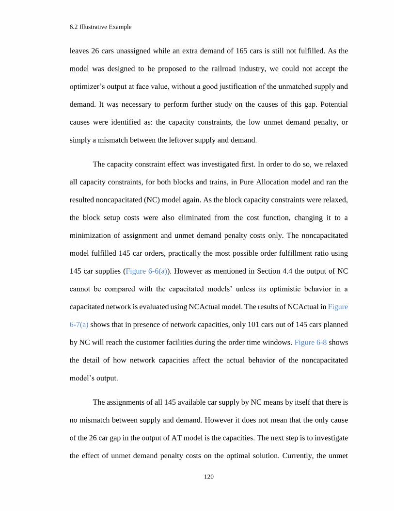
6.2 Illustrative Example
120
leaves 26 cars unassigned while an extra demand of 165 cars is still not fulfilled. As the
model was designed to be proposed to the railroad industry, we could not accept the
optimizer’s output at face value, without a good justification of the unmatched supply and
demand. It was necessary to perform further study on the causes of this gap. Potential
causes were identified as: the capacity constraints, the low unmet demand penalty, or
simply a mismatch between the leftover supply and demand.
The capacity constraint effect was investigated first. In order to do so, we relaxed
all capacity constraints, for both blocks and trains, in Pure Allocation model and ran the
resulted noncapacitated (NC) model again. As the block capacity constraints were relaxed,
the block setup costs were also eliminated from the cost function, changing it to a
minimization of assignment and unmet demand penalty costs only. The noncapacitated
model fulfilled 145 car orders, practically the most possible order fulfillment ratio using
145 car supplies (Figure 6-6(a)). However as mentioned in Section 4.4 the output of NC
cannot be compared with the capacitated models’ unless its optimistic behavior in a
capacitated network is evaluated using NCActual model. The results of NCActual in Figure
6-7(a) shows that in presence of network capacities, only 101 cars out of 145 cars planned
by NC will reach the customer facilities during the order time windows. Figure 6-8 shows
the detail of how network capacities affect the actual behavior of the noncapacitated
model’s output.
The assignments of all 145 available car supply by NC means by itself that there is
no mismatch between supply and demand. However it does not mean that the only cause
of the 26 car gap in the output of AT model is the capacities. The next step is to investigate
the effect of unmet demand penalty costs on the optimal solution. Currently, the unmet

6.2 Illustrative Example
121
demand unit costs (ranged between 757 and 1446 and averaged at 1043 for days that
customers placed orders), compared to the assignment unit costs, (ranged between 50 and
1461 and averaged at 1135), are not high enough to enforce the assignment over shortage
for high-cost supply-order assignments. In order to analyze the effect of penalty costs, we
ran the PA and AT models again, but this time using higher penalty costs, where the least
penalty cost was larger than the biggest assignment cost. The results changed considerably.
In the new optimal solution of AT, 129 cars were assigned to the orders, lowering the gap
from 26 to 16. Further increase in shortage penalties did not improve the fulfillment ratio,
confirming that the only cause of the extra 19 car gap between the maximum possible
fulfilments (145 cars) and the AT output (129 cars) is the capacities of the network. The
details on the assignments suggested by all path based models using high penalty costs are
presented in Figure 6-4(b) to Figure 6-7(b).
Among the three above mentioned causes, the penalty costs seem to be of more
importance. The mismatch (not a cause here) comes from the nature of supply and demand
and we are almost empty handed against it. The capacity constraints are enforced by the
network and should not be relaxed especially after we saw that the optimistic behavior of
NC in capacitated network NCActual (assigning 101 cars in both low or high shortage cost
cases) is worse than the output of AT (assigning 119 cars in low shortage cost case and 129
cars in case of high shortage costs). The unmet demand penalties however are part of the
model parameters and we have more control over them.
While fulfilling 129 orders, using the high penalty costs in the Allocation-Timing
model, compared to fulfilling only 119 orders using the initial penalty costs, might seem
more interesting to the Car Distribution Department and customers; it is important to assure

6.2 Illustrative Example
122
that these assignments are also profitable. Railroad carriers, in general, charge their
customers based on the number of miles and days it takes to deliver the loaded cars from
customer facility to the requested destination and not by the number of empty cars they
sent to them nor the number of days and miles it takes the empty cars to reach the customer
facility (similar to taxi drivers!). While customers will also benefit from a better fleet
utilization, minimizing the empty miles is more in the railroad interest compared to the
customers’ interest. As an extreme case, consider that there is only one empty car available
in Albany, New York, and two customers requested it: a customer located at Jacksonville,
Florida, and a local customer in Upstate New York. Is it profitable (with respect to short
term or long term considerations) to ship the car all the way to the South to satisfy the
customer demand? The answer depends on many factors, among them how important and
how profitable the customer in Florida is for the railroad carrier (Please see Section 3.2.5
for the details on cost function).

6.2 Illustrative Example
123
(a)
(b)
Figure 6-4 Detailed supply-order assignment suggested by PA with a) low shortage and
b) high shortage penalties
1 2 3 4 5 6 7 1 2 3 4 5 6 7 1 2 3 4 5 6 7 1 2 3 4 5 6 7
2.
000
1.
414
1.
000
0.
707
0.
500
0.
354
0.
250
2.
000
1.
414
1.
000
0.
707
0.
500
0.
354
0.
250
2.
000
1.
414
1.
000
0.
707
0.
500
0.
354
0.
250
1.
000
0.
707
0.
500
0.
354
0.
250
0.
177
0.
125
2169
1745
1446
1234
1084
979
904
2019
1625
1346
1149
1009
911
841
2169
1745
1446
1234
1084
979
904
1346
1149
1009
911
841
792
757
Pure Allocation Model (PA)
4227 1 0 0 0 0 0 0 0 0 0 0 0 0 1 0 0 0 0 0 0 0 0 0 0 0 0 0 0 0 5 1 4
4227 3 0 0 0 3 0 3 0 0 0 0 0 0 0 0 0 0 0 0 0 0 0 0 0 0 0 0 0 0 20 6 14
8765 1 0 0 0 0 13 11 0 0 0 0 0 0 0 0 0 0 0 0 0 0 0 0 0 0 0 0 0 0 24 24 -
8765 3 0 0 3 0 0 1 0 0 0 0 0 0 0 0 0 0 0 0 0 0 0 0 0 0 0 0 0 0 4 4 -
10588 1 0 0 0 0 0 0 0 0 0 0 0 0 0 0 0 0 0 0 0 0 0 0 0 0 0 0 0 0 3 - 3
10588 3 0 0 0 0 0 2 0 0 0 0 0 0 0 2 0 0 0 0 0 0 0 0 0 0 0 0 0 0 15 4 11
4227 4 0 0 0 0 0 0 0 0 0 0 0 0 0 0 0 0 0 0 0 0 0 0 0 0 0 0 0 0 12 - 12
4227 6 0 0 0 0 0 0 0 0 0 0 0 0 0 0 0 0 0 3 0 0 0 0 0 0 0 0 0 0 20 3 17
2474 4 0 0 0 0 0 0 0 0 0 0 0 0 0 0 0 0 0 0 0 7 4 0 0 0 0 0 0 0 20 11 9
2474 6 0 0 0 0 0 0 0 0 0 0 0 0 0 0 0 0 0 0 0 0 6 0 0 0 0 0 0 0 6 6 -
8429 4 0 0 0 0 0 0 0 0 0 0 0 0 0 0 0 0 0 0 5 0 0 0 0 0 0 0 4 0 12 9 3
8429 6 0 0 0 0 0 0 0 0 0 0 0 0 0 0 0 0 0 0 4 0 0 0 0 0 0 0 0 0 4 4 -
145 72 73
0 0 3 8 15 21 26 0 0 2 6 12 17 21 0 0 4 9 17 25 30 0 0 3 7 14 20 24 284
0 0 3 3 13 17 0 0 0 0 0 0 1 2 0 0 0 3 9 7 10 0 0 0 0 0 4 0 72
0 0 0 5 2 4 26 0 0 2 6 12 16 19 0 0 4 6 8 18 20 0 0 3 7 14 16 24 212
0 0 0 5 2 1 14 0 0 0 0 5 5 12 0 0 2 5 6 6 10 0 0 1 4 6 10 11 105
Demand (d_n)
Satisfied
Shortage (y_n)
Soft bound (y_n_max)
SUPP
LY
Car
Typ
e 1
carT
ype2
Ass
igne
d
Lef
t
Customer: 1, Yard:1954,
K_n:{1,3}, Pref:(2,1)}
Customer:2, Yard:1339,
K_n:{1,3}, Pref:(1,1)}
Customer: 3, Yard:6872,
K_n:{4,6}, Pref:(2,1)}
Customer: 4, Yard:2040,
K_n:{4,6}, Pref:(1,1)}
Sup
ply
(s-m
-k)
Day
Priority
Shortage penalty
(c_n, c'_n)
DEMAND (284 cars)
Yard
Po
ol (
k)
Car Type 1 (131 cars) Car Type 2 (153 cars)
1 2 3 4 5 6 7 1 2 3 4 5 6 7 1 2 3 4 5 6 7 1 2 3 4 5 6 7
2.
000
1.
414
1.
000
0.
707
0.
500
0.
354
0.
250
2.
000
1.
414
1.
000
0.
707
0.
500
0.
354
0.
250
2.
000
1.
414
1.
000
0.
707
0.
500
0.
354
0.
250
1.
000
0.
707
0.
500
0.
354
0.
250
0.
177
0.
125
4338
3490
2892
2468
2168
1958
1808
4038
3250
2692
2298
2018
1822
1682
4338
3490
2892
2468
2168
1958
1808
2692
2298
2018
1822
1682
1584
1514
Pure Allocation Model (PA)
4227 1 0 0 0 0 0 0 0 0 0 0 0 0 1 0 0 0 0 0 0 0 0 0 0 0 0 0 0 0 5 1 4
4227 3 0 0 0 3 3 0 0 0 0 0 0 0 0 0 0 0 0 0 0 0 0 0 0 0 0 0 0 0 20 6 14
8765 1 0 0 0 0 10 14 0 0 0 0 0 0 0 0 0 0 0 0 0 0 0 0 0 0 0 0 0 0 24 24 -
8765 3 0 0 3 0 0 1 0 0 0 0 0 0 0 0 0 0 0 0 0 0 0 0 0 0 0 0 0 0 4 4 -
10588 1 0 0 0 0 0 0 0 0 0 0 0 0 0 0 0 0 0 0 0 0 0 0 0 0 0 0 0 0 3 - 3
10588 3 0 0 0 0 0 2 0 0 0 0 0 0 0 2 0 0 0 0 0 0 0 0 0 0 0 0 0 0 15 4 11
4227 4 0 0 0 0 0 0 0 0 0 0 0 0 0 0 0 0 0 0 0 0 0 0 0 0 0 0 0 0 12 - 12
4227 6 0 0 0 0 0 0 0 0 0 0 0 0 0 0 0 0 0 3 0 0 0 0 0 0 0 0 0 0 20 3 17
2474 4 0 0 0 0 0 0 0 0 0 0 0 0 0 0 0 0 0 0 0 7 4 0 0 0 0 0 0 0 20 11 9
2474 6 0 0 0 0 0 0 0 0 0 0 0 0 0 0 0 0 0 0 0 0 6 0 0 0 0 0 0 0 6 6 -
8429 4 0 0 0 0 0 0 0 0 0 0 0 0 0 0 0 0 0 0 5 0 0 0 0 0 0 0 4 0 12 9 3
8429 6 0 0 0 0 0 0 0 0 0 0 0 0 0 0 0 0 0 0 4 0 0 0 0 0 0 0 0 0 4 4 -
145 72 73
0 0 3 8 15 21 26 0 0 2 6 12 17 21 0 0 4 9 17 25 30 0 0 3 7 14 20 24 284
0 0 3 3 13 17 0 0 0 0 0 0 1 2 0 0 0 3 9 7 10 0 0 0 0 0 4 0 72
0 0 0 5 2 4 26 0 0 2 6 12 16 19 0 0 4 6 8 18 20 0 0 3 7 14 16 24 212
0 0 0 5 2 1 14 0 0 0 0 5 5 12 0 0 2 5 6 6 10 0 0 1 4 6 10 11 105
Demand (d_n)
Satisfied
Shortage (y_n)
Soft bound (y_n_max)
SUPP
LY
Car
Typ
e 1
carT
ype2
Ass
igne
d
Lef
t
Customer: 1, Yard:1954,
K_n:{1,3}, Pref:(2,1)}
Customer:2, Yard:1339,
K_n:{1,3}, Pref:(1,1)}
Customer: 3, Yard:6872,
K_n:{4,6}, Pref:(2,1)}
Customer: 4, Yard:2040,
K_n:{4,6}, Pref:(1,1)}
Sup
ply
(s-m
-k)
Day
Priority
Shortage penalty
(c_n, c'_n)
DEMAND (284 cars)
Yard
Po
ol (
k)
Car Type 1 (131 cars) Car Type 2 (153 cars)

6.2 Illustrative Example
124
(a)
(b)
Figure 6-5 Detailed supply-order assignment suggested by AT with a) low shortage and
b) high shortage penalties
1 2 3 4 5 6 7 1 2 3 4 5 6 7 1 2 3 4 5 6 7 1 2 3 4 5 6 7
2.
000
1.
414
1.
000
0.
707
0.
500
0.
354
0.
250
2.
000
1.
414
1.
000
0.
707
0.
500
0.
354
0.
250
2.
000
1.
414
1.
000
0.
707
0.
500
0.
354
0.
250
1.
000
0.
707
0.
500
0.
354
0.
250
0.
177
0.
125
2169
1745
1446
1234
1084
979
904
2019
1625
1346
1149
1009
911
841
2169
1745
1446
1234
1084
979
904
1346
1149
1009
911
841
792
757
Allocation-Timing Model (AT)
4227 1 0 0 0 0 4 1 0 0 0 0 0 0 0 0 0 0 0 0 0 0 0 0 0 0 0 0 0 0 5 5 -
4227 3 0 0 0 0 0 13 7 0 0 0 0 0 0 0 0 0 0 0 0 0 0 0 0 0 0 0 0 0 20 20 -
8765 1 0 0 3 7 5 2 0 0 0 0 0 7 0 0 0 0 0 0 0 0 0 0 0 0 0 0 0 0 24 24 -
8765 3 0 0 0 0 4 0 0 0 0 0 0 0 0 0 0 0 0 0 0 0 0 0 0 0 0 0 0 0 4 4 -
10588 1 0 0 0 0 0 0 0 0 0 0 0 0 0 0 0 0 0 0 0 0 0 0 0 0 0 0 0 0 3 - 3
10588 3 0 0 0 0 0 4 5 0 0 0 0 0 0 2 0 0 0 0 0 0 0 0 0 0 0 0 0 0 15 11 4
4227 4 0 0 0 0 0 0 0 0 0 0 0 0 0 0 0 0 0 0 0 0 0 0 0 0 0 0 0 0 12 - 12
4227 6 0 0 0 0 0 0 0 0 0 0 0 0 0 0 0 0 0 3 0 6 4 0 0 0 0 0 0 0 20 13 7
2474 4 0 0 0 0 0 0 0 0 0 0 0 0 0 0 0 0 0 0 0 8 10 0 0 0 0 2 0 0 20 20 -
2474 6 0 0 0 0 0 0 0 0 0 0 0 0 0 0 0 0 0 0 0 0 6 0 0 0 0 0 0 0 6 6 -
8429 4 0 0 0 0 0 0 0 0 0 0 0 0 0 0 0 0 0 0 9 3 0 0 0 0 0 0 0 0 12 12 -
8429 6 0 0 0 0 0 0 0 0 0 0 0 0 0 0 0 0 0 0 2 2 0 0 0 0 0 0 0 0 4 4 -
145 119 26
0 0 3 8 15 21 26 0 0 2 6 12 17 21 0 0 4 9 17 25 30 0 0 3 7 14 20 24 284
0 0 3 7 13 20 12 0 0 0 0 7 0 2 0 0 0 3 11 19 20 0 0 0 0 2 0 0 119
0 0 0 1 2 1 14 0 0 2 6 5 17 19 0 0 4 6 6 6 10 0 0 3 7 12 20 24 165
0 0 0 5 2 1 14 0 0 0 0 5 5 12 0 0 2 5 6 6 10 0 0 1 4 6 10 11 105
Demand (d_n)
Satisfied
Shortage (y_n)
Soft bound (y_n_max)
SUPP
LY
Car
Typ
e 1
carT
ype2
Ass
igne
d
Lef
t
Customer: 1, Yard:1954,
K_n:{1,3}, Pref:(2,1)}
Customer:2, Yard:1339,
K_n:{1,3}, Pref:(1,1)}
Customer: 3, Yard:6872,
K_n:{4,6}, Pref:(2,1)}
Customer: 4, Yard:2040,
K_n:{4,6}, Pref:(1,1)}
Sup
ply
(s-m
-k)
Day
Priority
Shortage penalty
(c_n, c'_n)
DEMAND (284 cars)
Yard
Po
ol (
k)
Car Type 1 (131 cars) Car Type 2 (153 cars)
1 2 3 4 5 6 7 1 2 3 4 5 6 7 1 2 3 4 5 6 7 1 2 3 4 5 6 7
2.
000
1.
414
1.
000
0.
707
0.
500
0.
354
0.
250
2.
000
1.
414
1.
000
0.
707
0.
500
0.
354
0.
250
2.
000
1.
414
1.
000
0.
707
0.
500
0.
354
0.
250
1.
000
0.
707
0.
500
0.
354
0.
250
0.
177
0.
125
4338
3490
2892
2468
2168
1958
1808
4038
3250
2692
2298
2018
1822
1682
4338
3490
2892
2468
2168
1958
1808
2692
2298
2018
1822
1682
1584
1514
Allocation-Timing Model (AT)
4227 1 0 0 0 0 1 3 1 0 0 0 0 0 0 0 0 0 0 0 0 0 0 0 0 0 0 0 0 0 5 5 -
4227 3 0 0 0 3 4 8 5 0 0 0 0 0 0 0 0 0 0 0 0 0 0 0 0 0 0 0 0 0 20 20 -
8765 1 0 0 3 0 2 4 0 0 0 0 0 7 8 0 0 0 0 0 0 0 0 0 0 0 0 0 0 0 24 24 -
8765 3 0 0 0 0 4 0 0 0 0 0 0 0 0 0 0 0 0 0 0 0 0 0 0 0 0 0 0 0 4 4 -
10588 1 0 0 0 0 0 0 0 0 0 0 0 0 0 3 0 0 0 0 0 0 0 0 0 0 0 0 0 0 3 3 -
10588 3 0 0 0 0 2 5 6 0 0 0 0 0 0 2 0 0 0 0 0 0 0 0 0 0 0 0 0 0 15 15 -
4227 4 0 0 0 0 0 0 0 0 0 0 0 0 0 0 0 0 0 0 0 0 0 0 0 0 0 0 0 0 12 - 12
4227 6 0 0 0 0 0 0 0 0 0 0 0 0 0 0 0 0 0 6 0 6 4 0 0 0 0 0 0 0 20 16 4
2474 4 0 0 0 0 0 0 0 0 0 0 0 0 0 0 0 0 0 0 0 7 11 0 0 0 0 2 0 0 20 20 -
2474 6 0 0 0 0 0 0 0 0 0 0 0 0 0 0 0 0 0 0 0 1 5 0 0 0 0 0 0 0 6 6 -
8429 4 0 0 0 0 0 0 0 0 0 0 0 0 0 0 0 0 0 0 7 5 0 0 0 0 0 0 0 0 12 12 -
8429 6 0 0 0 0 0 0 0 0 0 0 0 0 0 0 0 0 0 0 4 0 0 0 0 0 0 0 0 0 4 4 -
145 129 16
0 0 3 8 15 21 26 0 0 2 6 12 17 21 0 0 4 9 17 25 30 0 0 3 7 14 20 24 284
0 0 3 3 13 20 12 0 0 0 0 7 8 5 0 0 0 6 11 19 20 0 0 0 0 2 0 0 129
0 0 0 5 2 1 14 0 0 2 6 5 9 16 0 0 4 3 6 6 10 0 0 3 7 12 20 24 155
0 0 0 5 2 1 14 0 0 0 0 5 5 12 0 0 2 5 6 6 10 0 0 1 4 6 10 11 105
Demand (d_n)
Satisfied
Shortage (y_n)
Soft bound (y_n_max)
SUPP
LY
Car
Typ
e 1
carT
ype2
Ass
igne
d
Lef
t
Customer: 1, Yard:1954,
K_n:{1,3}, Pref:(2,1)}
Customer:2, Yard:1339,
K_n:{1,3}, Pref:(1,1)}
Customer: 3, Yard:6872,
K_n:{4,6}, Pref:(2,1)}
Customer: 4, Yard:2040,
K_n:{4,6}, Pref:(1,1)}
Sup
ply
(s-m
-k)
Day
Priority
Shortage penalty
(c_n, c'_n)
DEMAND (284 cars)
Yard
Po
ol (
k)
Car Type 1 (131 cars) Car Type 2 (153 cars)
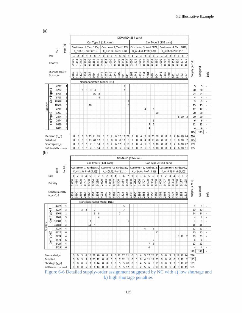
6.2 Illustrative Example
125
(a)
(b)
Figure 6-6 Detailed supply-order assignment suggested by NC with a) low shortage and
b) high shortage penalties
1 2 3 4 5 6 7 1 2 3 4 5 6 7 1 2 3 4 5 6 7 1 2 3 4 5 6 7
2.
000
1.
414
1.
000
0.
707
0.
500
0.
354
0.
250
2.
000
1.
414
1.
000
0.
707
0.
500
0.
354
0.
250
2.
000
1.
414
1.
000
0.
707
0.
500
0.
354
0.
250
1.
000
0.
707
0.
500
0.
354
0.
250
0.
177
0.
125
2169
1745
1446
1234
1084
979
904
2019
1625
1346
1149
1009
911
841
2169
1745
1446
1234
1084
979
904
1346
1149
1009
911
841
792
757
Noncapacitated Model (NC)
4227 1 0 0 0 0 0 0 0 0 0 0 0 0 5 0 0 0 0 0 0 0 0 0 0 0 0 0 0 0 5 5 -
4227 3 0 0 3 3 3 4 0 0 0 0 0 0 7 0 0 0 0 0 0 0 0 0 0 0 0 0 0 0 20 20 -
8765 1 0 0 0 0 0 16 8 0 0 0 0 0 0 0 0 0 0 0 0 0 0 0 0 0 0 0 0 0 24 24 -
8765 3 0 0 0 0 0 0 4 0 0 0 0 0 0 0 0 0 0 0 0 0 0 0 0 0 0 0 0 0 4 4 -
10588 1 0 0 0 0 0 0 0 0 0 0 0 0 0 3 0 0 0 0 0 0 0 0 0 0 0 0 0 0 3 3 -
10588 3 0 0 0 0 10 0 0 0 0 0 0 0 0 5 0 0 0 0 0 0 0 0 0 0 0 0 0 0 15 15 -
4227 4 0 0 0 0 0 0 0 0 0 0 0 0 0 0 0 0 0 4 0 8 0 0 0 0 0 0 0 0 12 12 -
4227 6 0 0 0 0 0 0 0 0 0 0 0 0 0 0 0 0 0 0 0 0 20 0 0 0 0 0 0 0 20 20 -
2474 4 0 0 0 0 0 0 0 0 0 0 0 0 0 0 0 0 0 0 0 0 0 0 0 0 0 8 10 2 20 20 -
2474 6 0 0 0 0 0 0 0 0 0 0 0 0 0 0 0 0 0 0 0 6 0 0 0 0 0 0 0 0 6 6 -
8429 4 0 0 0 0 0 0 0 0 0 0 0 0 0 0 0 0 0 0 7 5 0 0 0 0 0 0 0 0 12 12 -
8429 6 0 0 0 0 0 0 0 0 0 0 0 0 0 0 0 0 0 0 4 0 0 0 0 0 0 0 0 0 4 4 -
145 145 -
0 0 3 8 15 21 26 0 0 2 6 12 17 21 0 0 4 9 17 25 30 0 0 3 7 14 20 24 284
0 0 3 3 13 20 12 0 0 0 0 0 12 8 0 0 0 4 11 19 20 0 0 0 0 8 10 2 145
0 0 0 5 2 1 14 0 0 2 6 12 5 13 0 0 4 5 6 6 10 0 0 3 7 6 10 22 139
0 0 0 5 2 1 14 0 0 0 0 5 5 12 0 0 2 5 6 6 10 0 0 1 4 6 10 11 105
Satisfied
Shortage (y_n)
Soft bound (y_n_max)
SUPP
LY
Car
Typ
e 1
carT
ype2
Demand (d_n)
Ass
igne
d
Lef
t
Customer: 1, Yard:1954,
K_n:{1,3}, Pref:(2,1)}
Customer:2, Yard:1339,
K_n:{1,3}, Pref:(1,1)}
Customer: 3, Yard:6872,
K_n:{4,6}, Pref:(2,1)}
Customer: 4, Yard:2040,
K_n:{4,6}, Pref:(1,1)}
Sup
ply
(s-m
-k)
Day
Priority
Shortage penalty
(c_n, c'_n)
DEMAND (284 cars)
Yard
Po
ol (
k)
Car Type 1 (131 cars) Car Type 2 (153 cars)
1 2 3 4 5 6 7 1 2 3 4 5 6 7 1 2 3 4 5 6 7 1 2 3 4 5 6 7
2.
000
1.
414
1.
000
0.
707
0.
500
0.
354
0.
250
2.
000
1.
414
1.
000
0.
707
0.
500
0.
354
0.
250
2.
000
1.
414
1.
000
0.
707
0.
500
0.
354
0.
250
1.
000
0.
707
0.
500
0.
354
0.
250
0.
177
0.
125
4338
3490
2892
2468
2168
1958
1808
4038
3250
2692
2298
2018
1822
1682
4338
3490
2892
2468
2168
1958
1808
2692
2298
2018
1822
1682
1584
1514
Noncapacitated Model (NC)
4227 1 0 0 0 0 0 0 0 0 0 0 0 0 5 0 0 0 0 0 0 0 0 0 0 0 0 0 0 0 5 5 -
4227 3 0 0 3 3 0 7 0 0 0 0 0 0 7 0 0 0 0 0 0 0 0 0 0 0 0 0 0 0 20 20 -
8765 1 0 0 0 0 0 9 8 0 0 0 0 7 0 0 0 0 0 0 0 0 0 0 0 0 0 0 0 0 24 24 -
8765 3 0 0 0 0 0 0 4 0 0 0 0 0 0 0 0 0 0 0 0 0 0 0 0 0 0 0 0 0 4 4 -
10588 1 0 0 0 0 2 0 0 0 0 0 0 0 0 1 0 0 0 0 0 0 0 0 0 0 0 0 0 0 3 3 -
10588 3 0 0 0 0 11 4 0 0 0 0 0 0 0 0 0 0 0 0 0 0 0 0 0 0 0 0 0 0 15 15 -
4227 4 0 0 0 0 0 0 0 0 0 0 0 0 0 0 0 0 0 4 0 8 0 0 0 0 0 0 0 0 12 12 -
4227 6 0 0 0 0 0 0 0 0 0 0 0 0 0 0 0 0 0 0 0 0 20 0 0 0 0 0 0 0 20 20 -
2474 4 0 0 0 0 0 0 0 0 0 0 0 0 0 0 0 0 0 0 0 0 0 0 0 0 0 8 10 2 20 20 -
2474 6 0 0 0 0 0 0 0 0 0 0 0 0 0 0 0 0 0 0 0 6 0 0 0 0 0 0 0 0 6 6 -
8429 4 0 0 0 0 0 0 0 0 0 0 0 0 0 0 0 0 0 0 7 5 0 0 0 0 0 0 0 0 12 12 -
8429 6 0 0 0 0 0 0 0 0 0 0 0 0 0 0 0 0 0 0 4 0 0 0 0 0 0 0 0 0 4 4 -
145 145 -
0 0 3 8 15 21 26 0 0 2 6 12 17 21 0 0 4 9 17 25 30 0 0 3 7 14 20 24 284
0 0 3 3 13 20 12 0 0 0 0 7 12 1 0 0 0 4 11 19 20 0 0 0 0 8 10 2 145
0 0 0 5 2 1 14 0 0 2 6 5 5 20 0 0 4 5 6 6 10 0 0 3 7 6 10 22 139
0 0 0 5 2 1 14 0 0 0 0 5 5 12 0 0 2 5 6 6 10 0 0 1 4 6 10 11 105
Satisfied
Shortage (y_n)
Soft bound (y_n_max)
SUPP
LY
Car
Typ
e 1
carT
ype2
Demand (d_n)
Ass
igne
d
Lef
t
Customer: 1, Yard:1954,
K_n:{1,3}, Pref:(2,1)}
Customer:2, Yard:1339,
K_n:{1,3}, Pref:(1,1)}
Customer: 3, Yard:6872,
K_n:{4,6}, Pref:(2,1)}
Customer: 4, Yard:2040,
K_n:{4,6}, Pref:(1,1)}
Sup
ply
(s-m
-k)
Day
Priority
Shortage penalty
(c_n, c'_n)
DEMAND (284 cars)
Yard
Po
ol (
k)
Car Type 1 (131 cars) Car Type 2 (153 cars)

6.2 Illustrative Example
126
(a) (b)
Figure 6-7 Detailed supply-order assignment suggested by NCActual with a) low
shortage and b) high shortage penalties
1 2 3 4 5 6 7 1 2 3 4 5 6 7 1 2 3 4 5 6 7 1 2 3 4 5 6 7
2.
000
1.
414
1.
000
0.
707
0.
500
0.
354
0.
250
2.
000
1.
414
1.
000
0.
707
0.
500
0.
354
0.
250
2.
000
1.
414
1.
000
0.
707
0.
500
0.
354
0.
250
1.
000
0.
707
0.
500
0.
354
0.
250
0.
177
0.
125
2169
1745
1446
1234
1084
979
904
2019
1625
1346
1149
1009
911
841
2169
1745
1446
1234
1084
979
904
1346
1149
1009
911
841
792
757
Noncapacitated Model - Actual (NCActual)
4227 1 0 0 0 0 0 0 0 0 0 0 0 0 0 0 0 0 0 0 0 0 0 0 0 0 0 0 0 0 5 - 5
4227 3 0 0 3 3 3 4 0 0 0 0 0 0 0 0 0 0 0 0 0 0 0 0 0 0 0 0 0 0 20 13 7
8765 1 0 0 0 0 0 16 8 0 0 0 0 0 0 0 0 0 0 0 0 0 0 0 0 0 0 0 0 0 24 24 -
8765 3 0 0 0 0 0 0 4 0 0 0 0 0 0 0 0 0 0 0 0 0 0 0 0 0 0 0 0 0 4 4 -
10588 1 0 0 0 0 0 0 0 0 0 0 0 0 0 3 0 0 0 0 0 0 0 0 0 0 0 0 0 0 3 3 -
10588 3 0 0 0 0 5 0 0 0 0 0 0 0 0 2 0 0 0 0 0 0 0 0 0 0 0 0 0 0 15 7 8
4227 4 0 0 0 0 0 0 0 0 0 0 0 0 0 0 0 0 0 4 0 6 0 0 0 0 0 0 0 0 12 10 2
4227 6 0 0 0 0 0 0 0 0 0 0 0 0 0 0 0 0 0 0 0 0 4 0 0 0 0 0 0 0 20 4 16
2474 4 0 0 0 0 0 0 0 0 0 0 0 0 0 0 0 0 0 0 0 0 0 0 0 0 0 7 5 2 20 14 6
2474 6 0 0 0 0 0 0 0 0 0 0 0 0 0 0 0 0 0 0 0 6 0 0 0 0 0 0 0 0 6 6 -
8429 4 0 0 0 0 0 0 0 0 0 0 0 0 0 0 0 0 0 0 7 5 0 0 0 0 0 0 0 0 12 12 -
8429 6 0 0 0 0 0 0 0 0 0 0 0 0 0 0 0 0 0 0 4 0 0 0 0 0 0 0 0 0 4 4 -
145 101 44
0 0 3 8 15 21 26 0 0 2 6 12 17 21 0 0 4 9 17 25 30 0 0 3 7 14 20 24 284
0 0 3 3 8 20 12 0 0 0 0 0 0 5 0 0 0 4 11 17 4 0 0 0 0 7 5 2 101
0 0 0 5 7 1 14 0 0 2 6 12 17 16 0 0 4 5 6 8 26 0 0 3 7 7 15 22 183
0 0 0 5 2 1 14 0 0 0 0 5 5 12 0 0 2 5 6 6 10 0 0 1 4 6 10 11 105 Soft bound (y_n_max)
Demand (d_n)
Satisfied
Shortage (y_n)
SUPP
LY
Car
Typ
e 1
carT
ype2
Ass
igne
d
Lef
t
Customer: 1, Yard:1954,
K_n:{1,3}, Pref:(2,1)}
Customer:2, Yard:1339,
K_n:{1,3}, Pref:(1,1)}
Customer: 3, Yard:6872,
K_n:{4,6}, Pref:(2,1)}
Customer: 4, Yard:2040,
K_n:{4,6}, Pref:(1,1)}
Sup
ply
(s-m
-k)
Day
Priority
Shortage penalty
(c_n, c'_n)
DEMAND (284 cars)
Yard
Po
ol (
k)
Car Type 1 (131 cars) Car Type 2 (153 cars)
1 2 3 4 5 6 7 1 2 3 4 5 6 7 1 2 3 4 5 6 7 1 2 3 4 5 6 7
2.
000
1.
414
1.
000
0.
707
0.
500
0.
354
0.
250
2.
000
1.
414
1.
000
0.
707
0.
500
0.
354
0.
250
2.
000
1.
414
1.
000
0.
707
0.
500
0.
354
0.
250
1.
000
0.
707
0.
500
0.
354
0.
250
0.
177
0.
125
4338
3490
2892
2468
2168
1958
1808
4038
3250
2692
2298
2018
1822
1682
4338
3490
2892
2468
2168
1958
1808
2692
2298
2018
1822
1682
1584
1514
Noncapacitated Model - Actual (NCActual)
4227 1 0 0 0 0 0 0 0 0 0 0 0 0 0 0 0 0 0 0 0 0 0 0 0 0 0 0 0 0 5 - 5
4227 3 0 0 3 3 0 7 0 0 0 0 0 0 0 0 0 0 0 0 0 0 0 0 0 0 0 0 0 0 20 13 7
8765 1 0 0 0 0 0 9 8 0 0 0 0 7 0 0 0 0 0 0 0 0 0 0 0 0 0 0 0 0 24 24 -
8765 3 0 0 0 0 0 0 4 0 0 0 0 0 0 0 0 0 0 0 0 0 0 0 0 0 0 0 0 0 4 4 -
10588 1 0 0 0 0 0 0 0 0 0 0 0 0 0 1 0 0 0 0 0 0 0 0 0 0 0 0 0 0 3 1 2
10588 3 0 0 0 0 5 4 0 0 0 0 0 0 0 0 0 0 0 0 0 0 0 0 0 0 0 0 0 0 15 9 6
4227 4 0 0 0 0 0 0 0 0 0 0 0 0 0 0 0 0 0 4 0 6 0 0 0 0 0 0 0 0 12 10 2
4227 6 0 0 0 0 0 0 0 0 0 0 0 0 0 0 0 0 0 0 0 0 4 0 0 0 0 0 0 0 20 4 16
2474 4 0 0 0 0 0 0 0 0 0 0 0 0 0 0 0 0 0 0 0 0 0 0 0 0 0 7 5 2 20 14 6
2474 6 0 0 0 0 0 0 0 0 0 0 0 0 0 0 0 0 0 0 0 6 0 0 0 0 0 0 0 0 6 6 -
8429 4 0 0 0 0 0 0 0 0 0 0 0 0 0 0 0 0 0 0 7 5 0 0 0 0 0 0 0 0 12 12 -
8429 6 0 0 0 0 0 0 0 0 0 0 0 0 0 0 0 0 0 0 4 0 0 0 0 0 0 0 0 0 4 4 -
145 101 44
0 0 3 8 15 21 26 0 0 2 6 12 17 21 0 0 4 9 17 25 30 0 0 3 7 14 20 24 284
0 0 3 3 5 20 12 0 0 0 0 7 0 1 0 0 0 4 11 17 4 0 0 0 0 7 5 2 101
0 0 0 5 10 1 14 0 0 2 6 5 17 20 0 0 4 5 6 8 26 0 0 3 7 7 15 22 183
0 0 0 5 2 1 14 0 0 0 0 5 5 12 0 0 2 5 6 6 10 0 0 1 4 6 10 11 105 Soft bound (y_n_max)
Demand (d_n)
Satisfied
Shortage (y_n)
SUPP
LY
Car
Typ
e 1
carT
ype2
Ass
igne
d
Lef
t
Customer: 1, Yard:1954,
K_n:{1,3}, Pref:(2,1)}
Customer:2, Yard:1339,
K_n:{1,3}, Pref:(1,1)}
Customer: 3, Yard:6872,
K_n:{4,6}, Pref:(2,1)}
Customer: 4, Yard:2040,
K_n:{4,6}, Pref:(1,1)}
Sup
ply
(s-m
-k)
Day
Priority
Shortage penalty
(c_n, c'_n)
DEMAND (284 cars)
Yard
Po
ol (
k)
Car Type 1 (131 cars) Car Type 2 (153 cars)

6.2 Illustrative Example
127
Figure 6-8 Optimal assignment from noncapacitated model and its optimistic behavior

6.3 Performance of Models and Solution Procedures in Larger Scale Problems
128
A high level comparison of the model performance measures in two scenarios of
low or high shortage penalties is presented in Table 6-4. The huge difference between the
optimal objective values of the two scenarios for each model in Table 6-4 is because of the
high weight of shortage costs in the objective function. Hence the optimal cost of scenario
2, with less shortages comparing to Scenario 1 is considerably higher as a result of its
higher shortage penalty costs! This will justify the high cost of 441968 compared to 278653
for the same number of order fulfillment of 145 in NC. Another point to mention is the
difference between the objective value of AR and NC in Scenario 2 (respectively 459178
and 441968) with a similar fulfillment of 145 cars. Such a gap is expectable for two
reasons: 1) AR has capacity limitations practically having a smaller feasible region
compared to NC; and 2) NC does not consider block setup costs, resulting in a lower
objective value.
Table 6-4 Performance measures (optimal assigned cars; optimal objective value) for
different models for two scenarios with different shortage penalties
Sc. 1 Medium penalty
on shortage Sc. 2 High penalty
on shortage
Pure Allocation Model (PA) 72; 351546 72; 648629
Allocation-Timing Model (AT) 119; 309354 129; 503206
Allocation-Routing Model (AR) 138; 296584 145; 459178
Noncapacitated Model (NC) 145; 278653 145; 441968
NC on capacitated network (NCActual) 101; 331910 101; 578649
6.3 Performance of Models and Solution Procedures in Larger Scale
Problems
The illustrative example presented in Section 6.2 was small enough to be solved
using MIP solver of CPLEX software in about a second. However as the number of supply
nodes and demand profiles increased, CPLEX started to show the signs of fatigue! The run

6.3 Performance of Models and Solution Procedures in Larger Scale Problems
129
time for a problem with 20 supply nodes and 20 demand profiles was about 2 minutes and
it increased to more than 5 minutes after scaling the size to 40 supply nodes and 40 demand
profiles. The blocking network presented in Section 6.2, the Medium Network, has only
78 yards, and it is too small to be used for measuring the efficiency of the models on larger
scale. In this section we first explain the black box of the procedure that we use to generate
case examples. Then using case examples generated by this procedure, we perform some
sensitivity analysis tests and finally study the average performance of the proposed
heuristics in a variety of problem sizes.
Table 6-5 Different models, variable setup and algorithms to solve them
Form
ulatio
n
Problem Name Solution Procedure Flow
var. (x)
Block
setup
var. (z)
Path-
Based
Non-Capacitated
(NC)
NC-IP (CPLEX MIP Solver) Integer Binary
NCActual Integer Binary
Pure Allocation
(PA)
PA-IP (CPLEX MIP Solver) Integer Binary
Allocation-Timing
(AT)
AT-IP (CPLEX MIP Solver) Integer Binary
AT-LRH (Lagrangian Heuristic) Integer Binary
AT-MBP (Mixed Binary Programming) Cont+ Binary
AT-MBPRound (Rounding of MBP) Integer Binary
AT-IRRH1 (Iterative Relaxation and Rounding
Heuristic based on MBP setup)
Integer Binary
AT-LPRelax (Linear Programming Relaxation) Cont+ Cont+
AT-LPRound (Linear Programming Rounding) Integer Binary
AT-IRRH2 (Iterative Relaxation and Rounding
Heuristic based on LP setup)
Integer Binary
Arc-
Based
Allocation-
Routing (AR)
AR-IP Integer Binary

6.3 Performance of Models and Solution Procedures in Larger Scale Problems
130
Before we proceed with the next section, we need to introduce some notation that
we will use in this chapter referring to different models and algorithms. Table 6-5 contains
such notation. For example, in the first row NC stands for the Non-Capacitated model. NC-
IP refers to this model when it is solved using CPLEX built-in IP and MIP algorithms. The
last two columns state that the flow variables are integer while block setup variables are
binary (and none of them are relaxed).
6.3.1 Generating case examples
In this section, we first describe the input data components and then present the
case example generation procedure.
6.3.1.1 Input
Network- The efficiency of the models and algorithms were validated in a bigger
network, “Large Network”, with 440 yards, 1369 blocks, 624 trains and 2167 train
segments which in an 18-day time horizon results in 34941 nodes, 24642 blocks, 11232
trains and 39005 train segments (please see Section 6.1 for the characteristics of different
networks used for verification and validation purposes). The block and train capacities
come from RAS 2011 datasets. We use RAS block and train capacities as original
capacities. However, at any point of time, there are many loaded and empty cars already
planned for movement which occupy part of network’s original capacity. The residual
capacity of block 𝑏 is expressed as ratio of available capacity to its original capacity.
Knowing that the majority of capacity of a block for day 1 is expected to be already booked
by the empty and loaded cars planned before the current run of model, this ratio is assumed
to be a monotonically increasing function of time (for example ratio(t) = min(100, (5 + 5 *
t))/100). The residual capacities of trains are calculated in a similar way.

6.3 Performance of Models and Solution Procedures in Larger Scale Problems
131
𝑣𝑏 = 𝑣𝑏𝑜𝑟𝑖𝑔𝑖𝑛𝑎𝑙
∗ 𝑟𝑎𝑡𝑖𝑜(𝑡) (6-2)
𝑢𝑔 = 𝑢𝑔𝑜𝑟𝑖𝑔𝑖𝑛𝑎𝑙
∗ 𝑟𝑎𝑡𝑖𝑜(𝑡) (6-3)
where 𝑡 is the block/train departure day. This network will be used as input to generate
case examples. In a case example some blocks might have block setup costs. If a block
has a setup cost, which also means it is not yet constructed, its residual capacity should be
equal to its original capacity, regardless of the day it is associated with.
𝑣𝑏 = {𝑣𝑏𝑜𝑟𝑖𝑔𝑖𝑛𝑎𝑙
∗ 𝑟𝑎𝑡𝑖𝑜(𝑡), 𝑓𝑏 = 0
𝑣𝑏𝑜𝑟𝑖𝑔𝑖𝑛𝑎𝑙
, 𝑓𝑏 > 0 (6-4)
Demand- Demand is generated based on a Logistic function which is a
monotonically increasing bounded function and is defined by (6-5) and is illustrated in
Figure 6-9. In this function 𝑑(𝑡) is customer demand on day 𝑡, 𝑑𝑚𝑎𝑥 is the maximum daily
demand for this customer, and 𝑎 and 𝑡0 are the Logistic function parameters representing
the steepness of the curve and the day associated with demand midpoint, respectively.
𝑑(𝑡) = 𝑑𝑚𝑎𝑥/(1 + 𝑒−𝑎(𝑡−𝑡0)) (6-5)
The car distribution models presented in this dissertation, suggest supply to order
assignment decisions in a two-week time horizon and give higher priority to the earlier
days compared to later days, meaning that a customer’s demand for Monday has higher
priority than the same customer’s demand for Tuesday of the same week. Hence a demand
that was originally submitted to be fulfilled for today is most likely to be already (partially
or fully) fulfilled/planned by the previous runs of the model, while a demand for 10 days
from now has less chance to be fulfilled before the current run. This is why at each point
of time the unfulfilled (modified) demand so far that should be considered as the demand

6.3 Performance of Models and Solution Procedures in Larger Scale Problems
132
for the current run is expected to be close to zero for day 1 and close to its original demand
for day 14 and this is exactly what a logistic demand function generates.
Figure 6-9 Logistic function for creating daily demand
Finally the algorithm to generate 𝑛 number of demand profiles (customers) along
with their attributes such as eligible pools and preferences and daily demands is presented
below:
Algorithm for generating demand
INPUT: n = numDemandProfiles; Demand parameters (𝑎, 𝑡0, 𝑑𝑙,𝑑𝑢); C =
setOfCarTypes
Iterate for n times:
Uniformly pick a yard
𝑑(𝑡) = 40/(1 + 𝑒−1(𝑡−5))
𝑑𝑚𝑎𝑥 = 40
𝑡0 = 5
Demand
Day
𝑑𝑢 = 60
𝑑𝑙 = 30

6.3 Performance of Models and Solution Procedures in Larger Scale Problems
133
Uniformly assign a car type from C
Uniformly pick a set of pools within this car type
Uniformly assign pool preferences from {1,2,3}
Uniformly pick customer priority for day 1 (priority(Day 1)= uni{1,2,3}
Priority (Day t) = priority (Day t-1) /sqrt(2)
Calculate daily demand based on the logistic function given parameters (𝑎, 𝑡0, 𝑑𝑙,𝑑𝑢)
o 𝑑𝑚𝑎𝑥 = 𝑢𝑛𝑖(𝑑𝑙, 𝑑𝑢) =𝑢𝑛𝑖 (𝑚𝑎𝑥𝐷𝑒𝑚𝑎𝑛𝑑𝑙𝑜𝑤𝑒𝑟𝐵𝑜𝑢𝑛𝑑, 𝑚𝑎𝑥𝐷𝑒𝑚𝑎𝑛𝑑𝑢𝑝𝑝𝑒𝑟𝐵𝑜𝑢𝑛𝑑)
o 𝑑(𝑡) = 𝑑𝑚𝑎𝑥/(1 + 𝑒−𝑎(𝑡−𝑡0)) o Calculate the shortage penalties (see Section 3.2.5)
Supply- Total supply of cars for each car type is not necessarily equal to the total
demand for that car type. It is often less, since we usually want to allocate the current
supply to the demand for a two-week time horizon. Given the total demand of a particular
car type and the ratio between supply and demand, the total supply of the car type can be
easily calculated. Given that 𝑚 is the number of yards that have excess of supply of this
car type, 𝑚 yards are uniformly selected and the total supply of the car type is then
distributed, uniformly, in the 𝑚 yards and between all pools inside this car type. The
algorithm is as follows:
Algorithm for generating supply
INPUT: C = setOfCarTypes; m = numSupplyNodes ; r = supToDemRatio;
For each car type c in C:
TotalDemandOfCarType (c) = ∑ 𝑑(𝑡)1≤𝑡≤14 where requested pools are
in car type c
s = totalSupplyOfCarType(c) = TotalDemandOfCarType (c) * r
uniformly pick m yards
uniformly distribute s number of cars between pools in car type c in this
m yards
6.3.1.2 Procedure for generating case examples
In this section we present a procedure to generate case examples for simulation
purposes. Numbers inside parenthesis are only an example.

6.3 Performance of Models and Solution Procedures in Larger Scale Problems
134
INPUT: Network = Large Network (time-space), along with its capacities both original
(𝑣𝑏𝑜𝑟𝑖𝑔𝑖𝑛𝑎𝑙
, 𝑢𝑔𝑜𝑟𝑖𝑔𝑖𝑛𝑎𝑙
) and residual (𝑣𝑏 , 𝑢𝑔); c_maxBlockFixedCost (= 3000); case parameters
(a) to (k) and scenario parameters (l) and (m):
(a) double ratioOfBlocksWithSetupCost (= 0.2)
(b) int numCarTypes (= 2)
(c) int numPoolsInCarType (= 2)
(d) int numDemandProfiles (= 100)
(e) int maxDemand_lowerBound (= 30)
(f) int maxDemand_upperBound (= 50)
(g) int acceptedDelay (= 1)
(h) double steepnessLogistic (= 1)
(i) int midpointLogistic (= 5)
(j) int numSupplyNodes (= 150)
(k) double supToDemRatio (= 0.5)
(l) double shortagePenaltyCostFactor (= 1)
(m) double capFactor (= 1)
generateCaseExample (Network , c_maxBlockFixedCost,
ratioOfBlocksWithSetupCost, numCarType, numPoolInCarType, numDemandProfiles,
maxDemand_lowerBound, maxDemand_upperBound, acceptedDelay,
steepnessLogistic, midpointLogistic, numSupplyNodes, suptoDemRatio,
shortagePenaltyCostFactor, capFactor)
STEP 1 use (a) to calculate block setup costs. If block setup cost is not zero, reset the
block capacity to its original value based on equation (6-4).
𝑓𝑏 =
{𝑐_𝑚𝑎𝑥𝐵𝑙𝑜𝑐𝑘𝐹𝑖𝑥𝑒𝑑𝐶𝑜𝑠𝑡 ∗ (1 − 𝑟) , 𝑟 = 𝑢𝑛𝑖 (0, 1) < 𝑟𝑎𝑡𝑖𝑜𝑂𝑓𝐵𝑙𝑜𝑐𝑘𝑠𝑊𝑖𝑡ℎ𝑆𝑒𝑡𝑢𝑝𝐶𝑜𝑠𝑡
0 , 𝑜𝑡ℎ𝑒𝑟𝑤𝑖𝑠𝑒
𝑣𝑏 = 𝑣𝑏𝑜𝑟𝑖𝑔𝑖𝑛𝑎𝑙
𝑖𝑓 𝑓𝑏 > 0
STEP 2 use (b) to generate car type names (e.g. carType1, carType2)
STEP 3 use (c) to generate pools and assign them to car types (e.g. pools 1,2,3,4 were
1,2 are from carType1 and 3,4 are from carType2).
STEP 4 use parameters in (d-i) as parameters in “Algorithm for generating demand” in
Section 6.3.1.1 to generate demand.
STEP 5 use (j) and (k) as parameters in “Algorithm for generating supply” in Section
6.3.1.1 to generate supply
STEP 6 use (l) and (m) as scenario parameters to create different scenarios on the
generated case example
6.3.2 Sensitivity Analysis on Network Capacities
In addition to the number of nodes and arcs of the network and number of car types,
the size of the feasible region in Allocation-Timing model also depends on network
capacities. If network capacities are too high, compared to the supply and demand, they

6.3 Performance of Models and Solution Procedures in Larger Scale Problems
135
might become redundant and we might be able to relax them, practically solving the
Noncapacitated model. In this section the effect of network capacities on the objective
values and order fulfillment is analyzed. In order to do so first we developed a case example
using parameters listed in Table 6-6 and then applied our path-based models to this case
example in 10 different scenarios on network capacities ranged between 0.5 and 9.5 with
a step of 1 (everything else remains the same). The execution in each scenario was
terminated if the run time exceed 600 seconds or optimality gap was less than 1e-5. Figure
6-10 shows the performance measures (objective value, fulfilment, and run time) of
different path-based formulations for this case example. As one can see in Figure 6-10(a)
the Lagrangian Heuristic (AT-LRH) is not performing well and has a higher cost compared
to AT-IP which solves the same model using the built-in algorithms of CPLEX package.
In fact AT-LRH has the highest objective value at termination time in almost all cases. The
failure of AT-LRH might have two causes: a) the massive number of constraints, all train
and block capacity constraints, that are relaxed makes the LR severely infeasible that the
makeItFeasible() process is not able to find a feasible solution without dramatically
affecting the objective value and b) the construction times of creating subproblems is high
and the algorithm is terminated because of time limit without performing many iterations
towards optimality. In general we do not include the model construction times while
collecting the run times as a performance measure since it’s a onetime task and all models
have almost similar number of constraints and variables. However the subproblem
construction is part of LRH and the construction times cannot be excluded from the run
time. This is the reason we accept that this algorithm is not good for our problem.
Table 6-6 Parameters used to generate case example for sensitivity analysis

6.3 Performance of Models and Solution Procedures in Larger Scale Problems
136
Parameter Value
Network Large Network
ratioOfBlocksWithSetupCost 0.2
numCarType 5
numPoolInCarType 5
numDemandProfiles 100
maxDemand_lowerBound 20
maxDemand_upperBound 50
acceptedDelay 1
steepnessLogistic 1
midpointLogistic 5
numSupplyNodes 100
suptoDemRatio 0.25
shortagePenaltyCostFactor 1
capFactor 0.5-9.5
Stopping criteria 10min or epGap 1e-5
totalSupply 8538
totalDemand 36048
While AT-IP performs better than LRH, its performance is not acceptable in
general. If we compare this method with PA-IP whose feasible region is a subset of AT-
IP, we expect a superior performance (see Property 6-1a), while Figure 6-10(a) shows the
opposite! A short look at the run time in Figure 6-10(c) reveals that in all scenarios AT-IP
has terminated after 600 seconds and by reaching the time limit and not the optimality gap.
In other words Property 6-1a is not violated here since the optimal solution of AT-IP is not
reached. The main takeaway here is that solving the Allocation-Timing model using the
Lagrangian Heuristics or the CPLEX built-in algorithms, is not efficient enough to even
beat the solution suggested by Pure-Allocation model using CPLEX built-in algorithms.
The comparison between AT-IP and PA-IP should be sufficient to lead us to find
more efficient algorithms to solve the AT model. However to emphasize the importance of
such a need, we should compare the best algorithm so far, i.e. PA-IP, with the current
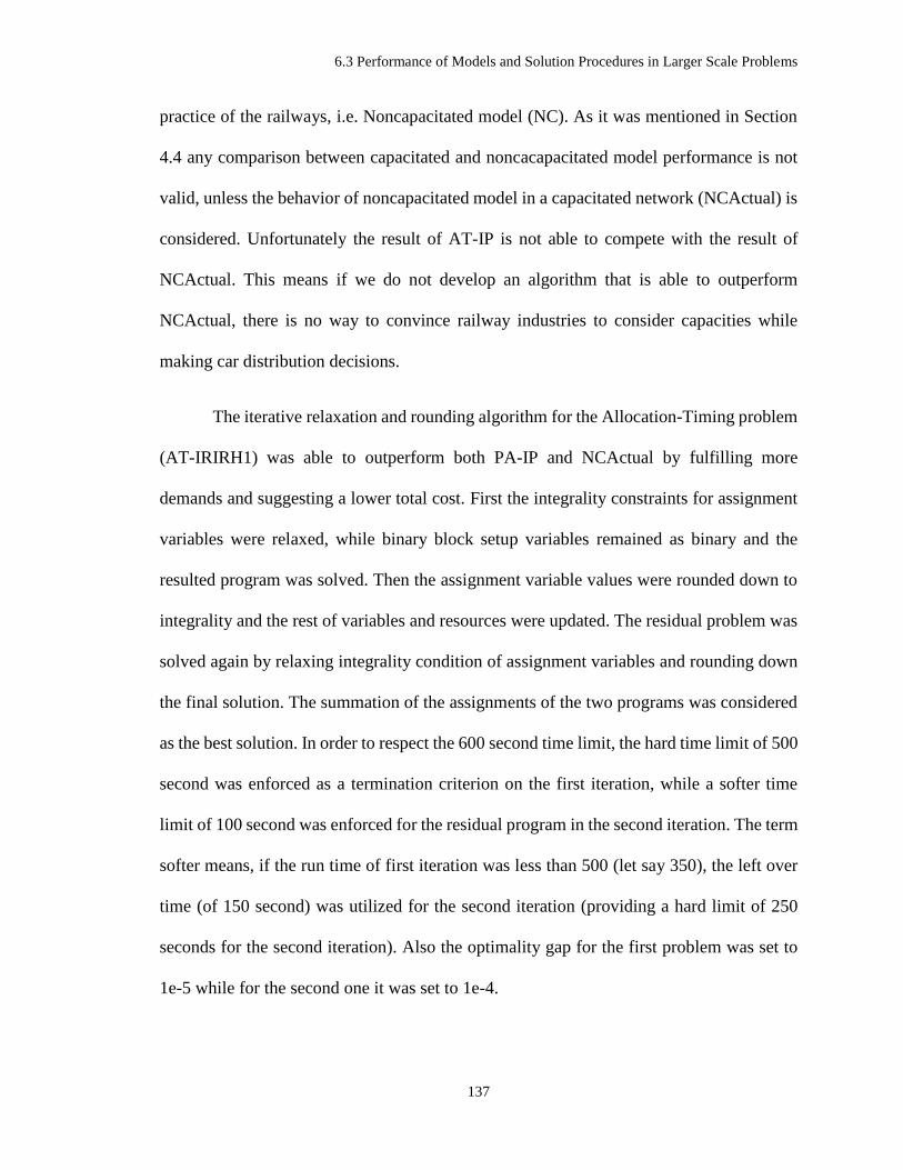
6.3 Performance of Models and Solution Procedures in Larger Scale Problems
137
practice of the railways, i.e. Noncapacitated model (NC). As it was mentioned in Section
4.4 any comparison between capacitated and noncacapacitated model performance is not
valid, unless the behavior of noncapacitated model in a capacitated network (NCActual) is
considered. Unfortunately the result of AT-IP is not able to compete with the result of
NCActual. This means if we do not develop an algorithm that is able to outperform
NCActual, there is no way to convince railway industries to consider capacities while
making car distribution decisions.
The iterative relaxation and rounding algorithm for the Allocation-Timing problem
(AT-IRIRH1) was able to outperform both PA-IP and NCActual by fulfilling more
demands and suggesting a lower total cost. First the integrality constraints for assignment
variables were relaxed, while binary block setup variables remained as binary and the
resulted program was solved. Then the assignment variable values were rounded down to
integrality and the rest of variables and resources were updated. The residual problem was
solved again by relaxing integrality condition of assignment variables and rounding down
the final solution. The summation of the assignments of the two programs was considered
as the best solution. In order to respect the 600 second time limit, the hard time limit of 500
second was enforced as a termination criterion on the first iteration, while a softer time
limit of 100 second was enforced for the residual program in the second iteration. The term
softer means, if the run time of first iteration was less than 500 (let say 350), the left over
time (of 150 second) was utilized for the second iteration (providing a hard limit of 250
seconds for the second iteration). Also the optimality gap for the first problem was set to
1e-5 while for the second one it was set to 1e-4.

6.3 Performance of Models and Solution Procedures in Larger Scale Problems
138
Since the AT-IRIRH1 was stopped by reaching the time limit in either the first or
the second iteration, its optimality is not guaranteed. In fact AT-IRIRH2 which uses the
linear programming relaxation provided better results in less time.
As you can see in Figure 6-10(b), when the capacity increases and the capacity
constraints become practically redundant, the AT-IRIRH algorithms for the capacitated
Allocation-Timing model provides a solution close to the one provided by the
noncapacitated model.

6.3 Performance of Models and Solution Procedures in Larger Scale Problems
139
a)
b)
c)
Figure 6-10 Path-Based formulation performance measures at the termination time when
capacity increases: a) objective value, b) order fulfillment, and c) run time

6.3 Performance of Models and Solution Procedures in Larger Scale Problems
140
6.3.3 Sensitivity Analysis on Shortage Penalties
As we saw in the Illustrative Example of Section 6.2, the optimal solution of the
car distribution models are influenced by the trade-off between assignment costs and the
shortage penalties. A model with high shortage penalties focuses on lowering the total
unmet demand and tries to not leave any supply unused while there is a demand for that,
unless it is not a good match. A model with lower shortage penalties, however, assigns a
car to an order only if its assignment cost is less than the penalty associated to the loss of
that demand.
In order to study the effect of shortage penalties on the order fulfillment ratio, we
consider the case problem of Section 6.3.2, but this time instead of changing the capacities,
we fix the capacity factor to 2.5 and changed the shortage penalty factor from 0.25 to 6.5,
with a step of 0.25 from 0.25 to 2.5 and a step of 1 from 2.5 to 6.5.3
Figure 6-11(b) shows that the order fulfilment for all models except AT-IP
increases when the shortage penalty factor increases from 0.25 to 1 and then remains almost
the same. Non-improvement of the order fulfilment in Figure 6-11(b), when shortage
penalty factor increases from 1 to 6.5, while dramatic increase in the objective value (cost)
confirms that our procedure for assigning values to the shortage penalties is well designed,
in such a way that the shortage penalties are big enough to guarantee the maximum order
fulfilments and not too big to overshoot the other components of the objective function
3 The shortage penalty factor was initially changed between 0.5 and 6.5 with a step of 1. However the
results showed that the order fulfillment is not affected after 2.5. This is why the effect of shortage penalty
factor was studied in more detail from 0.25 to 2.5 with a step of 0.25. The dramatic change of slope in
Figure 6-11(a) is a result of change of step size and does not have any insight attached to it.
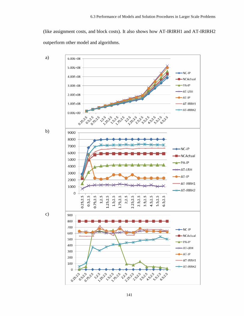
6.3 Performance of Models and Solution Procedures in Larger Scale Problems
141
(like assignment costs, and block costs). It also shows how AT-IRIRH1 and AT-IRIRH2
outperform other model and algorithms.
a)
b)
c)

6.3 Performance of Models and Solution Procedures in Larger Scale Problems
142
Figure 6-11 Path-Based formulation performance measures at the termination time when
shortage penalties increase: a) objective value, b) order fulfillment, and c) run time
6.3.4 Average Time Complexity of the Proposed Heuristic
Although the path-based car distribution problem, Allocation-Timing, was
formulated as an Integer Programming model, the Iterative Relaxation and Rounding
Heuristic (AT-IRRH2) presented in Section 4.3.3, repeatedly, solves the LP relaxation of
the problem and its residuals. The worst case complexity of simplex method is known to
be exponential; however it has a polynomial-time average complexity, under various
probability distributions (Spielman and Teng, 2004). In order to improve the efficiency of
the algorithm, we use the optimal basis of Pure Allocation model as the initial basis for
Allocation-Timing model. In this section we examine whether the average complexity of
AT-IRRH2 with initial basis is polynomial.
In order to analyze the average complexity of the algorithm, a number of
computational experiments were conducted. The number of car types, 𝑐, number of demand
profiles, 𝑛, and number of supply nodes, 𝑚, were used as variable input for generating
random instances of problems and all other parameters maintained the same for all cases
based on table Table 6-7 and all instances were generated on the same network: the Large
Network.
The model was run for 5 and 10 car types while the number of demand profiles and
number of supply nodes both varied from 10 to 200 with a step of 10 for 10 to 50 and a
step of 50 for 50 to 200.

6.3 Performance of Models and Solution Procedures in Larger Scale Problems
143
For each tuple of (𝑐, 𝑛,𝑚) values, 20 random instances were generated. The models
were applied to each random instance and in each run, performance measures were
collected and the average run time of the 20 runs for each problem size (𝑐, 𝑛, 𝑚)was
calculated.
Table 6-7 Parameters used to generate case examples for computational complexity
calculations
Parameter Value
Network Large Network
ratioOfBlocksWithSetupCost 0.2
numCarType 5, 10
numPoolInCarType 5
numDemandProfiles 10 to 200
maxDemand_lowerBound 30
maxDemand_upperBound 60
acceptedDelay 1
steepnessLogistic 1
midpointLogistic 5
numSupplyNodes 10 to 200
suptoDemRatio 0.5
shortagePenaltyCostFactor 1
capFactor 1
Stopping criteria (10min or epGap 1e-5) 25 min (1500 s) or epGap 1e-4
The hypothetical regression model was defined as a power law function:
𝑡 = 𝜆𝑐𝛼𝑛𝛽𝑚𝛾, (6-6)
where the run time 𝑡 is the response variable while the number of car types 𝑐, number of
demand profiles 𝑛, and number of supply nodes 𝑚 are the regressor variables. A
logarithmic transformation of (6-6), results in a multiple linear regression model:
𝑇 = Λ + 𝛼𝐶 + 𝛾𝑁 + 𝛽𝑀 (6-7)

6.3 Performance of Models and Solution Procedures in Larger Scale Problems
144
Where 𝑇 = 𝐿𝑛(𝑡), 𝐶 = 𝐿𝑛(𝑐), 𝑀 = 𝐿𝑛(𝑚), 𝑁 = 𝐿𝑛(𝑛) and Λ = 𝐿𝑛(𝜆) (and equivalently
𝜆 = 𝑒Λ).
By fitting the time data to a power trendline, the equation 𝑡 =
0.008164𝑐−0.3219𝑛1.3675𝑚1.1386 with 𝑅2 = 0.9 and adjusted 𝑅2 = 0.8834 was obtained
which confirms the polynomial average complexity of the algorithm. Figure 6-12 confirms
that the number of demand profiles and number of supply nodes have more effect on
solution time.
Figure 6-12 Average solution time of AT-IRRH2 with initial basis (solid green circles)
along with its estimation from the regression model (empty blue circles)
There is a negative power on the number of car types 𝑐, which means the run time
decreases as the number of car types increases, might seem nonsense at first look. However
after investigating the observed data, we noticed a similar trend. Further investigation
showed that the reverse relationship between the number of car types and the run time does
exist, and is originated from the procedure that we propose in Section 6.3.1.2 to generate
the case examples. When the number of supply nodes and the number of demand profiles

6.3 Performance of Models and Solution Procedures in Larger Scale Problems
145
as well as the distribution of supply and demand in each node are given, an increase in the
number of car types, without increasing the total supply or demand, will result in a higher
chance of mismatch between supply-order pairs and as a result less number of eligible paths
or equivalently less number of variables. For example, if there are only two customers,
each ordering only one car of car type 1 and we have a supply of two cars of car type 1
located at two different yards, then we can potentially have 4 eligible supply-order pairs.
While if we have the same number of customers, each ordering only one car but from two
different car types, then we will have a maximum of two supply-order pairs only. In fact 𝑛
can be written as 𝑛 = 𝑟 ∗ 𝑐 where 𝑟 is the average number of demand profile per car type.
The estimated run time function is transformed to 𝑡 =
0.008164𝑐1.0456𝑟1.3675𝑚1.1386which means including a new commodity, along with its
demand profiles, to the model will increase the solution time (almost linearly). Figure 6-13
shows that the power law model is a good fit for the average run time of the problem.
Figure 6-13 Average run time vs estimated run time from a power law model
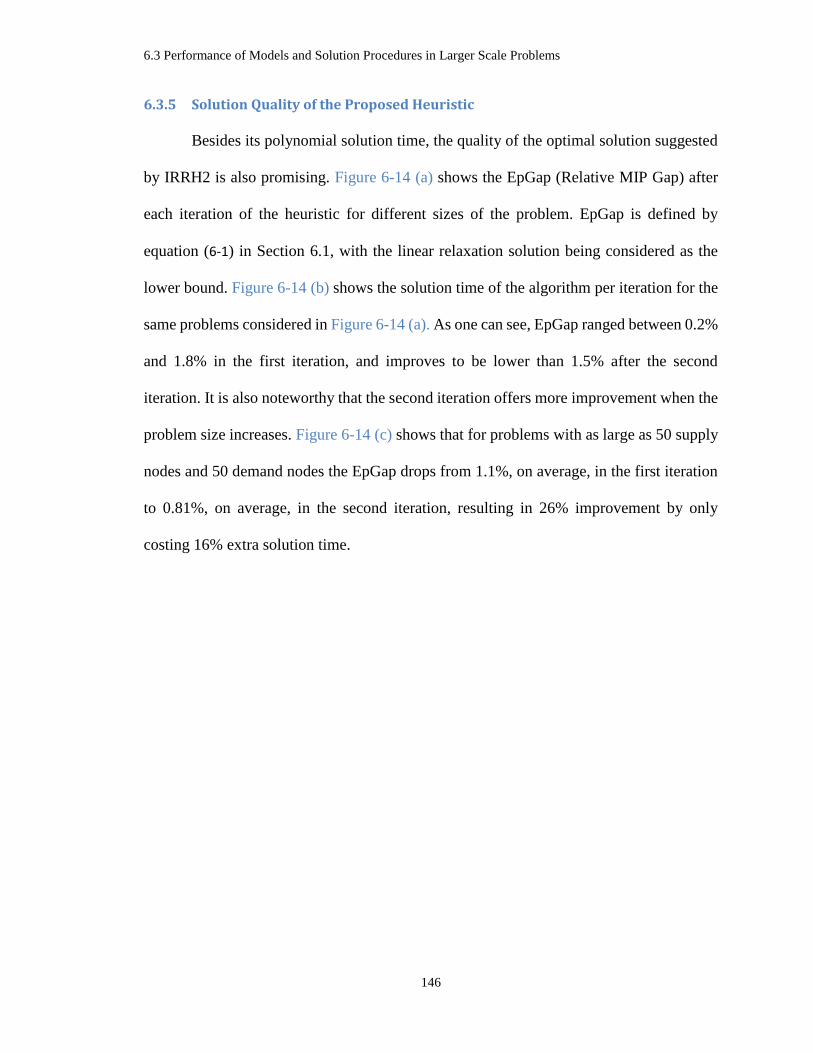
6.3 Performance of Models and Solution Procedures in Larger Scale Problems
146
6.3.5 Solution Quality of the Proposed Heuristic
Besides its polynomial solution time, the quality of the optimal solution suggested
by IRRH2 is also promising. Figure 6-14 (a) shows the EpGap (Relative MIP Gap) after
each iteration of the heuristic for different sizes of the problem. EpGap is defined by
equation (6-1) in Section 6.1, with the linear relaxation solution being considered as the
lower bound. Figure 6-14 (b) shows the solution time of the algorithm per iteration for the
same problems considered in Figure 6-14 (a). As one can see, EpGap ranged between 0.2%
and 1.8% in the first iteration, and improves to be lower than 1.5% after the second
iteration. It is also noteworthy that the second iteration offers more improvement when the
problem size increases. Figure 6-14 (c) shows that for problems with as large as 50 supply
nodes and 50 demand nodes the EpGap drops from 1.1%, on average, in the first iteration
to 0.81%, on average, in the second iteration, resulting in 26% improvement by only
costing 16% extra solution time.

6.3 Performance of Models and Solution Procedures in Larger Scale Problems
147
a)
b)
c)
Figure 6-14 The performance measures of IRRH2 per iteration when the problem size
increases. a) EpGap, b) solution time, and c) their trade-off
Average EpGap (MIP Gap) Run Time of AT-IRRH2 with initial basis
Iteration 1 Iteration 2 Improvement Relational
Improveme
nt
Run Time Iteration 1 Iteration 2 Relational
Extra time
AvgLargeScale 1.10% 0.81% 0.29% 26% 542 472 70 16%
stdLargeScale 0.41% 0.32% 0.17% 11% 330 290 40 3%

7.1 Summary
148
Chapter 7
7 Summary, Results and Future Research
7.1 Summary
Because of spatial and temporal imbalances in the supply and demand of empty
railcars/cars in freight transportation systems, empty equipment repositioning is inevitable.
As the owners of rail network, trains and railcars, railway carriers charge their customers
based on the days and the miles that a railcar is under load. Hence the cost of shipping
empty cars to customers as well as the opportunity cost of extra inventory in customer
facilities is on the railway’s shoulder. This is the reason why railway carriers have invested
a lot of money on optimizing their empty railcar distribution processes. For instance, CSX
invested $5 million to lunch their real-time car distribution system in 1997 (Gorman et al.,
2010), followed by BNSF's Equipment Distribution System which cost $3 million.
Despite the vast studies performed in the railroad optimization modeling, there is
still a need for another realistic modeling and optimization of the empty railcar distribution
problem. In particular, there is no previous work that optimizes the empty railcar
distribution decisions while simultaneously considering the resource (capacity)
availabilities in the service network and the car type substitutability for the customer

7.1 Summary
149
demands as well as separating the car distribution and car routing decision in accordance
to the US railroad practices.
In this research we developed two formulations for the Empty Railcar Distribution
problem, both aiming to minimize the total setup costs, total transportation costs, and total
shortage penalties under supply limitation, demand satisfaction, customer preferences and
priorities, and network capacity constraints.
We first formulated the problem as a path-based capacitated network flow model.
Contrary to the traditional path-based formulations, the path connecting each supply-
demand pair was given by an external application called Trip Planner which is defined on
top of a time-space network. Another application called Pseudo Path Generator then was
developed to generate alternative paths for each supply-order pair. Then we formulated the
problem as an arc-based capacitated multi-commodity network flow model where contrary
to the path-based model, the car routing and car distribution decisions were integrated in a
single model. Both models are complex and because of the huge number of constraints and
integer decision variables are hard to solve. However, the path-based formulation is more
practical for the United States railroads since in US railroad industry car routing and car
distribution decisions are separated from each other and usually made by different
departments.
Before prescribing the usage of our models, the models, computer programs and
solution procedures needed to be verified and validated. A computer program was
developed in Java and its accuracy was verified using debugging techniques, observational
verification and analytical verification (see Section 6.1). After verifying that the computer
program correctly represents the model, the next step was to validate the performance of

7.1 Summary
150
different models, especially our path based Allocation-Timing model, by benchmarking
them against each other and also against the noncapacitated model as the current practice
of many railway industries. Case examples used for validation purposes were generated on
a network called “Large Network” with 440 yards, 1369 blocks, 624 trains and 2167 train
segments which in an 18-day time horizon results in 34941 nodes, 24642 blocks, 11232
trains and 39005 train segments.
The models were implemented in Java and for small size problems solved using
Concert Technology of the IBM CPLEX solver. However as the number of supply nodes
and demand profiles increased, the solution time increased exponentially. The run time for
a problem with 20 supply nodes and 20 demand profiles was about 2 minutes while it
exceeded an hour after scaling the size to 100 supply nodes and 100 demand profiles. In
order to decrease the solution time of the path-based model, first we developed a
Lagrangian Heuristic (AT-LRH) and upon its failure we developed an Iterative Relaxation
and Rounding Heuristic (IRRH). In each iteration of IRRH, a subset of integrality
constraints was relaxed and the associated variables in the optimal solution of this relaxed
problem were rounded down. Then, the constraints were modified to reflect the residual
problem based on the rounded variables. Such an updated instance was passed to the next
iteration for further processing. The relaxation was performed in two different ways
resulting in two different heuristics: a) relaxing only the integer variables and keeping the
binary ones as they are (IRRH1) or b) relaxing all integer variables to general non-negative
variables and all binary variables to continuous variables between 0 and 1 (IRRH2).
7.2 Results
151
7.2 Results
The comparison of path-based and arc-based formulations in both capacitated and
uncapacitated modes confirmed the efficiency of the heuristic from both run time and
solution quality perspectives. The experiments in large-scale problems showed that AT-
LRH is not performing well and has a higher cost compared to AT-IP which solves the
same model using the built-in algorithms of CPLEX package. However since AT-IP was
terminated because of time limit and not because of reaching the optimal solution, it was
outperformed by PA-IP. The iterative relaxation and rounding algorithm for the Allocation-
Timing problem (AT-IRIRH1) outperformed PA-IP in both capacitated and noncapacitated
modes by fulfilling more demands and suggesting a lower total cost. AT-IRIRH2 proved
to be even more efficient than AT-IRIRH1. Furthermore, to improve the efficiency of AT-
IRIRH2, we used the optimal basis of Pure Allocation model as the initial basis for
Allocation-Timing model.
In order to analyze the average complexity of the algorithm, a number of
computational experiments were conducted. The number of car types, 𝑐, number of demand
profiles, 𝑛, and number of supply nodes, 𝑚, were used as variable input size parameters
for generating random instances of problems and the solution time for each instance was
collected. By fitting the solution time data to a power trendline, the equation 𝑡 =
0.008164𝑐−0.3219𝑛1.3675𝑚1.1386 with 𝑅2 = 0.9 and adjusted 𝑅2 = 0.8834 was obtained
which confirms the polynomial average complexity of the algorithm.
7.3 Future Research
Despite the above mentioned merits, the proposed models and algorithms point to
a number of directions for future research. The path-based AT problem presented in this

7.3 Future Research
152
research is a general integer programming model and its solution time, using integer
programming techniques, highly depends on the number of integer variable. In this
research we transformed the problem of finding all pseudo paths of a given trip plan, to
finding all permutations of a given word with two letters B and I. The number of paths and
consequently the number of assignment variables increase exponentially when the number
of blocks (B) in the trip plan or the number of days (I) in the planning horizon increases.
A smarter algorithm which builds only those pseudo paths that have higher chance of being
in the optimal solution, or at least fathoms those with almost no chance of being in the
optimal solution might help to lower the solution time of the integer programming models
and enable us to use the CPLEX solver to solve the problem directly.
Another issue regarding the Pseudo Path Generator is that it has been built under
the assumption that all trains operate regularly and repeat in the exact same time during all
the days of the week. In reality however, not all trains operate seven days a week nor they
are all on-time. A pseudo path generation algorithm that uses the actual train schedules
rather than simply repeating them in the same time during the week is more realistic.
Another contribution to this work could be developing solution techniques that do not
depend on licensed solver engines. This might be helpful in two ways. First, by saving the
licensing cost and second, by avoiding the incompatibility of newer versions of the
optimization software with the other applications interacting with solvers in the car
distribution system. Finally, the efficiency of proposed models and heuristics should be
verified on real work data in a pilot period, before implementing in railway industries.
153
References Ahmed, M., Lubiw, A., 2013. Shortest Paths Avoiding Forbidden Subpaths. Networks 61,
322–334. doi:10.1002/net.21490
Ahmed, M., Lubiw, A., 2009. Shortest Paths Avoiding Forbidden Subpaths. Proceedings
of the 26th International Symposium on Theoretical Aspects of Computer Science
63–74.
Ahuja, R.K., Magnanti, T.L., Orlin, J.B., 1993. Network Flows: Theory, Algorithms, and
Applications, 1 edition. ed. Prentice Hall, Englewood Cliffs, N.J.
AIAA, 1998. AIAA Guide for the Verification and Validation of Computational Fluid
Dynamics Simulations, AIAA-G-077-1998. American Institute of Aeronautics and
Astronautics.
Ballis, A., Dimitriou, L., 2010. Issues on Railway Wagon Asset Management Using
Advanced Information Systems. Transportation Research Part C: Emerging
Technologies 18, 807–820. doi:10.1016/j.trc.2009.09.003
Bandeira, D.L., Becker, J.L., Borenstein, D., 2009. A DSS for Integrated Distribution of
Empty and Full Containers. Decision Support Systems 47, 383–397.
doi:10.1016/j.dss.2009.04.003
Cao, C., Gao, Z., Li, K., 2008. The Empty Railcar Allocation Problem Under Uncertainty
for the Railway Freight Carrier, in: IEEE International Conference on Service
Operations and Logistics, and Informatics, 2008. IEEE/SOLI 2008. Presented at
the IEEE International Conference on Service Operations and Logistics, and
Informatics, 2008. IEEE/SOLI 2008, pp. 1512–1515.
doi:10.1109/SOLI.2008.4682765
7.3 Future Research
154
Choong, S.T., Cole, M.H., Kutanoglu, E., 2002. Empty Container Management for
Intermodal Transportation Networks. Transportation Research Part E: Logistics
and Transportation Review 38, 423–438. doi:10.1016/S1366-5545(02)00018-2
Crainic, T.G., 2003. Long-Haul Freight Transportation, in: Hall, R.W. (Ed.), Handbook of
Transportation Science, International Series in Operations Research &
Management Science. Springer US, pp. 451–516.
Crainic, T.G., Laporte, G., 1997. Planning Models for Freight Transportation. European
Journal of Operational Research 97, 409–438. doi:10.1016/S0377-2217(96)00298-
6
Dang, Q.-V., Yun, W.-Y., Kopfer, H., 2012. Positioning Empty Containers Under
Dependent Demand Process. Computers & Industrial Engineering, Soft Computing
for Management Systems 62, 708–715. doi:10.1016/j.cie.2011.11.021
Dantzig, G.B., 1951. Application of the Simplex Method to a Transportation Problem, in:
Tjalling C. Koopmans (Ed.), Activity Analysis of Production and Allocation. John
Wiley & Sons, Inc., New York, pp. 359–373.
Dejax, P.J., Crainic, T.G., 1987. Survey Paper-a Review of Empty Flows and Fleet
Management Models in Freight Transportation. Transportation Science 21, 227–
248.
Di Puglia Pugliese, L., Guerriero, F., 2011. Dynamic Programming Approaches to Solve
the Shortest Path Problem with Forbidden Paths. Optimization Methods and
Software 28, 221–255. doi:10.1080/10556788.2011.630077
155
Dong, J.-X., Song, D.-P., 2009. Container Fleet Sizing and Empty Repositioning in Liner
Shipping Systems. Transportation Research Part E: Logistics and Transportation
Review 45, 860–877. doi:10.1016/j.tre.2009.05.001
Engels, B., 2011. A Generalized Network Model for Freight Car Distribution (Ph.D.
Dissertation). Universität zu Köln.
Erera, A.L., Morales, J.C., Savelsbergh, M., 2009. Robust Optimization for Empty
Repositioning Problems. Operations Research 57, 468–483.
Ford, L.R., Jr., Fulkerson, D.R., 1956. Solving the Transportation Problem. Management
Science 3, 24–32.
Godfrey, G.A., Powell, W.B., 2002. An Adaptive Dynamic Programming Algorithm for
Dynamic Fleet Management, I: Single Period Travel Times. Transportation Science
36, 21–39.
Gorman, M.F., Acharya, D., Sellers, D., 2010. CSX Railway Uses OR to Cash In on
Optimized Equipment Distribution. Interfaces 40, 5–16.
doi:10.1287/inte.1090.0465
Gorman, M.F., Crook, K., Sellers, D., 2011. North American Freight Rail Industry Real-
Time Optimized Equipment Distribution Systems: State of the Practice.
Transportation Research Part C: Emerging Technologies 19, 103–114.
doi:10.1016/j.trc.2010.03.012
Haghani, A.E., 1989. Formulation and Solution of a Combined Train Routing and Makeup,
and Empty Car Distribution Model. Transportation Research Part B:
Methodological 23, 433–452. doi:10.1016/0191-2615(89)90043-X

7.3 Future Research
156
Haghani, A.E., 1987. Rail Freight Transportation: A Review of Recent Optimization
Models for Train Routing and Empty Car Distribution. J. Adv. Transp. 21, 147–
172. doi:10.1002/atr.5670210205
Herren, H., 1977. Computer-Controlled Empty Wagon Distribution on the SBB. RAIL
INTERNATIONAL 8, 25–32.
Holmberg, K., Joborn, M., Lundgren, J.T., 1998. Improved Empty Freight Car
Distribution. Transportation Science 32, 163–173.
Holmberg, K., Joborn, M., Melin, K., 2008. Lagrangian Based Heuristics for the
Multicommodity Network Flow Problem with Fixed Costs on Paths. European
Journal of Operational Research 188, 101–108. doi:10.1016/j.ejor.2007.04.029
Holmberg, K., Yuan, D., 2003. A Multicommodity Network-Flow Problem with Side
Constraints on Paths Solved by Column Generation. INFORMS Journal on
Computing 15, 42–57.
Jain, K., 2001. A Factor 2 Approximation Algorithm for the Generalized Steiner Network
Problem. Combinatorica 21, 39–60. doi:10.1007/s004930170004
Joborn, M., 2001. Optimization of Empty Freight Car Distribution in Scheduled Railways.
Division of Optimization, Department of Mathematics, Linköping University,
Linköping.
Joborn, M., Crainic, T.G., Gendreau, M., Holmberg, K., Lundgren, J.T., 2004. Economies
of Scale in Empty Freight Car Distribution in Scheduled Railways. Transportation
Science 38, 121–134. doi:10.1287/trsc.1030.0061
Jordan, W.C., Turnquist, M.A., 1983. A Stochastic, Dynamic Network Model for Railroad
Car Distribution. Transportation Science 17, 123–145. doi:10.1287/trsc.17.2.123

157
Lam, S.-W., Lee, L.-H., Tang, L.-C., 2007. An Approximate Dynamic Programming
Approach for the Empty Container Allocation Problem. Transportation Research
Part C: Emerging Technologies 15, 265–277. doi:10.1016/j.trc.2007.04.005
MAJER, T., 2011. An Algorithm for the Problem of Shortest Trail with Prohibited
Maneuvers. Journal of Information, Control and Management Systems 9.
Mesa-Arango, R., Ukkusuri, S., Sarmiento, I., 2013. Network Flow Methodology for
Estimating Empty Trips in Freight Transportation Models. Transportation Research
Record: Journal of the Transportation Research Board 2378, 110–119.
doi:10.3141/2378-12
Misra, S.C., 1972. Linear Programming of Empty Wagon Disposition. RAIL
INTERNATIONAL 3, 151–158.
Narisetty, A.K., Richard, J.-P.P., Ramcharan, D., Murphy, D., Minks, G., Fuller, J., 2008.
An Optimization Model for Empty Freight Car Assignment at Union Pacific
Railroad. Interfaces 38, 89–102. doi:10.1287/inte.1070.0330
Newman, A.M., Nozick, L.K., Yano, C.A., 2002. Optimization in the Rail Industry, in:
Pardalos, P.M., Resende, M.G.C. (Eds.), Handbook of Applied Optimization.
Oxford University Press, New York.
Ouimet, G.P., 1972. Empty Freight Car Distribution (M.Sc. Thesis). Queen’s University,
Kingston, Ontario, Canada.
Powell, W.B., 1987. An Operational Planning Model for the Dynamic Vehicle Allocation
Problem with Uncertain Demands. Transportation Research Part B:
Methodological 21, 217–232. doi:10.1016/0191-2615(87)90005-1

7.3 Future Research
158
Powell, W.B., Topaloglu, H., 2006. Approximate Dynamic Programming for Large-Scale
Resource Allocation Problems, in: Johnson, M.P., Norman, B., Secomandi, N.
(Eds.), Tutorials in Operations Research: Models, Methods, and Applications for
Innovative Decision Making. informs.
Sherali, H.D., Suharko, A.B., 1998. A Tactical Decision Support System for Empty Railcar
Management. Transportation Science 32, 306–329.
Song, D.-P., Dong, J.-X., 2013. Long-Haul Liner Service Route Design with Ship
Deployment and Empty Container Repositioning. Transportation Research Part B:
Methodological 55, 188–211. doi:10.1016/j.trb.2013.06.012
Spieckermann, S., Voß, S., 1995. A Case Study in Empty Railcar Distribution. European
Journal of Operational Research, Operational Research in Europe 87, 586–598.
doi:10.1016/0377-2217(95)00232-4
Spielman, D.A., Teng, S.-H., 2004. Smoothed Analysis of Algorithms: Why the Simplex
Algorithm Usually Takes Polynomial Time. J. ACM 51, 385–463.
doi:10.1145/990308.990310
Stanley, R.P., 2011. Enumerative Combinatorics: Volume 1, 2 edition. ed. Cambridge
University Press, Cambridge, NY.
Suharko, A.B., 1997. Tactical Network Flow and Discrete Optimization Models and
Algorithms for the Empty Railcar Transportation Problem (Ph.D. Dissertation).
Virginia Polytechnic Institute and State University.
Topaloglu, H., 2007. A Parallelizable and Approximate Dynamic Programming-Based
Dynamic Fleet Management Model with Random Travel Times and Multiple
Vehicle Types, in: Zeimpekis, V., Tarantilis, C.D., Giaglis, G.M., Minis, I. (Eds.),

159
Dynamic Fleet Management, Operations Research/Computer Science Interfaces
Series. Springer US, pp. 65–93.
Topaloglu, H., Powell, W.B., 2006. Dynamic-Programming Approximations for Stochastic
Time-Staged Integer Multicommodity-Flow Problems. INFORMS Journal on
Computing 18, 31–42. doi:10.1287/ijoc.1040.0079
Topaloglu, H., Powell, W.B., 2005. A Distributed Decision-Making Structure for Dynamic
Resource Allocation using Nonlinear Functional Approximations. Operations
Research 53, 281–297. doi:10.1287/opre.1040.0166
Turnquist, M.A., 1994. Economies of Scale and Network Optimization for Empty Car
Distribution (Technical Report). Cornell University, Ithaca, NY.
Turnquist, M.A., Markowicz, B.P., 1989. An Interactive Microcomputer-Based Planning
Model for Railroad Car Distribution. Presented at the CORS/ORSA/TIMS National
Meeting, Vancouver, BC.
Villeneuve, D., Desaulniers, G., 2005. The Shortest Path Problem with Forbidden Paths.
European Journal of Operational Research 165, 97–107.
doi:10.1016/j.ejor.2004.01.032
Wang, B., Wang, Z., 2007. Research on the Optimization of Intermodal Empty Container
Reposition of Land-carriage. Journal of Transportation Systems Engineering and
Information Technology 7, 29–33. doi:10.1016/S1570-6672(07)60020-8
White, W.W., 1972. Dynamic Transshipment Networks: An Algorithm and Its Application
to the Distribution of Empty Containers. Networks 2, 211–236.
doi:10.1002/net.3230020304

7.3 Future Research
160
White, W.W., Bomberault, A.M., 1969. A Network Algorithm for Empty Freight Car
Allocation. IBM Syst. J. 8, 147–169. doi:10.1147/sj.82.0147