
Optimised Distance Measurement with 3D-CMOS Image Sensor ... · Diskussionen wurde gemeinsam das...
156
Optimized Distance Measurement with 3D-CMOS Image Sensor and Real-Time Processing of the 3D Data for Applications in Automotive and Safety Engineering Von der Fakult¨ at f¨ ur Ingenieurwissenschaften der Universit¨ at Duisburg-Essen zur Erlangung des akademischen Grades eines Doktors der Ingenieurwissenschaften genehmigte Dissertation von Bernhard K¨ onig aus M¨ unchen Referent: Prof. Bedrich J. Hosticka, Ph.D. Korreferent: Prof. Dr. Josef Pauli Tag der m¨ undlichen Pr¨ ufung: 02.07.2008
Transcript of Optimised Distance Measurement with 3D-CMOS Image Sensor ... · Diskussionen wurde gemeinsam das...

Optimized Distance Measurement with 3D-CMOS
Image Sensor and Real-Time Processing of the 3D Data
for Applications in Automotive and Safety Engineering
Von der Fakultat fur Ingenieurwissenschaften der
Universitat Duisburg-Essen
zur Erlangung des akademischen Grades eines
Doktors der Ingenieurwissenschaften
genehmigte Dissertation
von
Bernhard Konig
aus Munchen
Referent: Prof. Bedrich J. Hosticka, Ph.D.
Korreferent: Prof. Dr. Josef Pauli
Tag der mundlichen Prufung: 02.07.2008

Vorwort
Diese Arbeit entstand im Rahmen der Zusammenarbeit zwischen dem Fraun-hofer Institut fur Mikroelektronische Schaltungen und Systeme(FhG IMS) in Duisburg und der Abteilung CT PS 9 von Siemens Coorpo-rate Technology in Munchen. Als externer Mitarbeiter von Siemens CT PS 9durfte ich im industriellen Forschungsumfeld an interessanten Projekten mit-arbeiten und die Forschungstatigkeiten meiner Promotion durchfuhren. Ichdanke Dr. Gunther Doemens und Dr. Claudio Laloni, den Abteilungsleiternvon Siemens CT PS 9, die mir dies ermoglicht haben.Genauso danke ich Prof. Bedrich J. Hosticka, Ph.D. vom FhG IMS fur dieBetreuung meiner Promotion. Er beobachtete stets den Fortschritt meinerArbeiten und unterstutzte mich durch sachkundige Ratschlage.Mein besonderer Dank gilt Dr. Peter Mengel, meinem Betreuer bei SiemensCT PS 9, sowie meinem Kollegen Ludwig Listl, deren fachkundige Anleitungwesentlich zum Gelingen dieser Arbeit beitrug. In vielen Fachgesprachen undDiskussionen wurde gemeinsam das Fundament fur diese Arbeit gelegt.Weiter mochte ich meinen Kollegen vom FhG IMS und von Siemens CT PS 9,Wiebke Ulfig, Dr. Omar Elkhalili, Uwe Phillipi und Roland Burger fur dieangenehme Zusammenarbeit, und meiner Familie und meinen Freunden furden Ausgleich zum Arbeitsumfeld danken.
Bernhard Konig
Munchen, 31. Oktober 2007
i

ii

Abstract
This thesis describes and characterizes an advanced range camera for the dis-tance range from 2 m to 25 m and novel real-time 3D image processing al-gorithms for object detection, tracking and classification on the basis of thethree-dimensional features of the camera output data.The technology is based on a 64x8 pixel array CMOS image sensor which iscapable of capturing three-dimensional images. This is accomplished by exe-cuting indirect time of flight measurement of NIR laser pulses emitted by thecamera and reflected by the objects in the field of view of the camera.An analytic description of the measurement signals and a derivation of thedistance measuring algorithms are conducted in this thesis as well as a com-parative examination of the distance measuring algorithms by calculation, sim-ulation and experiments; in doing so, the MDSI3 algorithm showed the best re-sults over the whole measurement range and is thus chosen as standard methodof the distance measuring system.A camera prototype was developed with a measurement accuracy in the cen-timeter range at an image repetition rate up to 100 Hz; a detailed evaluationof the components and of the over-all system is presented. Main aspects arethe characterization of the time critical measurement signals, of the systemnoise, and of the distance measuring capabilities.Furthermore this thesis introduces novel real-time image processing of the out-put data stream of the camera aiming at the detection of objects being locatedin the observed area and the derivation of reliable position, speed and accel-eration estimates. The used segmentation algorithm utilizes all three spatialdimensions of the position information as well as the intensity values and thusyields significant improvement compared to segmentation in conventional 2Dimages. Position, velocity, and acceleration values of the segmented objects areestimated by means of Kalman filtering in 3D space. The filter is dynamicallyadapted to the measurement properties of the according object to take care ofchanges of the data properties. The good performance of the image processingalgorithms is presented by means of example scenes.
iii

iv

Kurzfassung
Diese Arbeit beschreibt und charakterisiert eine neu entwickelte Entfernungs-kamera fur Reichweiten von 2 m bis 25 m und spezielle 3D-Echtzeit-Bildverar-beitungsalgorithmen zum Detektieren, Tracken und Klassifizieren von Objek-ten auf der Grundlage der dreidimensionalen Kameradaten.Die Technologie basiert auf einem 64x8 Pixel CMOS Bildsensor, welcher imStande ist, dreidimensionale Szenen zu erfassen. Dies wird mittels indirekterLaufzeitmessung von NIR Laserpulsen, die von der Kamera ausgesandt undan Objekten im Blickfeld der Kamera reflektiert werden, realisiert.Eine analytische Beschreibung der Messsignale und eine darauf aufbauendeHerleitung der verschiedenartigen Entfernungsmessungsalgorithmen wird indieser Arbeit ebenso durchgefuhrt, wie die vergleichende Betrachtung der Ent-fernungsmessungsalgorithmen durch Rechnung, Simulation und Experimente;dabei zeigt der MDSI3-Algorithmus die besten Ergebnisse uber den gesamtenMessbereich, und wird deshalb zum Standardalgorithmus des Entfernungs-messsystems.Ein Kameraprototyp mit Messgenauigkeiten im cm-Bereich bei einer Bild-wiederholrate bis zu 100 Hz wurde entwickelt; eine detaillierte Evaluierung derKomponenten und des Systems ist hier beschrieben. Hauptaspekte sind dabeidie Charakterisierung der zeitkritischen Messsignale, des Systemrauschens undder Entfernungsmesseigenschaften.Desweiteren wird in dieser Arbeit die neu entwickelte Echtzeit-Bildverarbeitungdes Kameradatenstroms vorgestellt, die auf die Detektion von Objekten imBeobachtungsbereich und die verlassliche Ermittlung von Positions-,Geschwin-digkeits- und Beschleunigungsschatzwerten abzielt. Der dabei verwendete Seg-mentierungsalgorithmus nutzt alle drei Dimensionen der Positionsmesswertekombiniert mit den Intensitatswerten der Messsignale, und liefert so eine sig-nifikante Verbesserung im Vergleich zur Segmentierung in konventionellen 2DBildern. Position, Geschwindigkeit und Beschleunigung werden mit Hilfe einesKalman-Filters im 3-dimensionalen Raum geschatzt. Das Filter passt sich dy-namisch den Messbedingungen des jeweils gemessenen Objekts an, und beruck-sichtigt so Veranderungen der Dateneigenschaften. Die Leistungsfahigkeit derBildverarbeitungsalgorithmen wird anhand von Beispielszenen demonstriert.
v

vi

Contents
Vorwort i
Abstract iii
Kurzfassung v
Table of Contents vii
1 Introduction 11.1 Motivation and Purpose . . . . . . . . . . . . . . . . . . . . . . 11.2 Structure of this Work . . . . . . . . . . . . . . . . . . . . . . . 3
2 Non-Contact Distance Measurement 52.1 Sonar and Radar . . . . . . . . . . . . . . . . . . . . . . . . . . 52.2 Optical Distance Measurement Techniques . . . . . . . . . . . . 7
2.2.1 Interferometry . . . . . . . . . . . . . . . . . . . . . . . . 72.2.2 Triangulation . . . . . . . . . . . . . . . . . . . . . . . . 8
2.2.2.1 Stereo Vision . . . . . . . . . . . . . . . . . . . 92.2.2.2 Active Triangulation / CCT . . . . . . . . . . . 10
2.2.3 Time of Flight Distance Measurement . . . . . . . . . . 112.2.3.1 Continuous Wave Methods . . . . . . . . . . . 122.2.3.2 Pulse Based Methods . . . . . . . . . . . . . . 13
2.2.3.2.1 Direct TOF Measurement . . . . . . . 132.2.3.2.2 Indirect TOF Measurement (3D-CMOS) 13
3 Theory of 3D-CMOS Distance Measurement 153.1 Measuring Principle . . . . . . . . . . . . . . . . . . . . . . . . . 153.2 Camera Optics . . . . . . . . . . . . . . . . . . . . . . . . . . . 163.3 Signal Generation . . . . . . . . . . . . . . . . . . . . . . . . . . 17
3.3.1 Pulsed Illumination . . . . . . . . . . . . . . . . . . . . . 173.3.2 Reflected Signal . . . . . . . . . . . . . . . . . . . . . . . 183.3.3 Short Time Integration . . . . . . . . . . . . . . . . . . . 19
vii

3.3.4 Integrator Output Signal . . . . . . . . . . . . . . . . . . 20
3.4 Distance Derivation Algorithms . . . . . . . . . . . . . . . . . . 21
3.4.1 MDSI . . . . . . . . . . . . . . . . . . . . . . . . . . . . 22
3.4.2 Gradient Method . . . . . . . . . . . . . . . . . . . . . . 25
3.4.3 CSI and DCSI . . . . . . . . . . . . . . . . . . . . . . . . 26
3.4.4 Conclusion . . . . . . . . . . . . . . . . . . . . . . . . . . 27
4 3D-CMOS Array Sensor System 29
4.1 System Components . . . . . . . . . . . . . . . . . . . . . . . . 30
4.1.1 Novel Array Sensor . . . . . . . . . . . . . . . . . . . . . 30
4.1.1.1 Pixel Structure . . . . . . . . . . . . . . . . . . 30
4.1.1.2 Correlated Double Sampling . . . . . . . . . . . 33
4.1.1.3 Analog Accumulation and Adaptive Accumu-lation . . . . . . . . . . . . . . . . . . . . . . . 33
4.1.1.4 Nondestructive Readout . . . . . . . . . . . . . 35
4.1.1.5 Sensor Control / Bit Pattern . . . . . . . . . . 35
4.1.2 Laser Illumination . . . . . . . . . . . . . . . . . . . . . 35
4.1.2.1 Laser Light Source . . . . . . . . . . . . . . . . 36
4.1.2.2 Beam Forming Optics . . . . . . . . . . . . . . 36
4.1.3 Imaging Optics / VOV . . . . . . . . . . . . . . . . . . . 36
4.1.4 Electronics . . . . . . . . . . . . . . . . . . . . . . . . . . 37
4.1.5 Firmware / Software . . . . . . . . . . . . . . . . . . . . 38
4.2 System Characterization . . . . . . . . . . . . . . . . . . . . . . 39
4.2.1 Image Sensor Characterization . . . . . . . . . . . . . . . 39
4.2.1.1 Responsivity . . . . . . . . . . . . . . . . . . . 39
4.2.1.2 Shutter Function . . . . . . . . . . . . . . . . . 41
4.2.1.3 Analog Accumulation . . . . . . . . . . . . . . 42
4.2.1.4 Optical / Electrical Crosstalk . . . . . . . . . . 43
4.2.2 Laser Illumination Characterization . . . . . . . . . . . . 44
4.2.2.1 Pulse Shape . . . . . . . . . . . . . . . . . . . . 44
4.2.2.2 Output Power . . . . . . . . . . . . . . . . . . . 45
4.2.2.3 Pulse Stability . . . . . . . . . . . . . . . . . . 45
4.2.2.4 Eye Safety . . . . . . . . . . . . . . . . . . . . . 47
4.2.3 Over-all System Characterization . . . . . . . . . . . . . 48
4.2.3.1 System Noise / System NEE . . . . . . . . . . 48
4.2.3.2 Shutter-Window-Pulse Correlation . . . . . . . 54
4.2.3.3 Dynamic Range . . . . . . . . . . . . . . . . . . 56
4.2.3.4 Distance Measurement Performance . . . . . . 59
4.2.3.5 Camera Frame Rate . . . . . . . . . . . . . . . 61
4.3 Camera Calibration . . . . . . . . . . . . . . . . . . . . . . . . . 61
4.3.1 Offset Calibration . . . . . . . . . . . . . . . . . . . . . . 61
4.3.2 Distance Calibration . . . . . . . . . . . . . . . . . . . . 62
viii

5 Optimization of the Distance Measurement 65
5.1 Comparison of the Distance Measurement Algorithms . . . . . . 65
5.1.1 Mathematical Investigation . . . . . . . . . . . . . . . . 65
5.1.1.1 Propagation of Uncertainties . . . . . . . . . . 66
5.1.2 Investigation using Simulation . . . . . . . . . . . . . . . 69
5.1.3 Experimental Results . . . . . . . . . . . . . . . . . . . . 69
5.2 Further Enhancement Approaches . . . . . . . . . . . . . . . . . 72
5.2.1 Treatment of Environmental Influences . . . . . . . . . . 72
5.2.1.1 Temperature Fluctuations . . . . . . . . . . . . 72
5.2.1.2 Ambient Light . . . . . . . . . . . . . . . . . . 72
5.2.1.3 Rain / Snowfall . . . . . . . . . . . . . . . . . . 73
5.2.2 Saturation Treatment . . . . . . . . . . . . . . . . . . . . 75
6 Novel 3D Real-Time Image Processing 79
6.1 Raw Data Properties . . . . . . . . . . . . . . . . . . . . . . . . 80
6.2 Coordinate Systems and Coordinate Transformations . . . . . . 80
6.2.1 Pixel and Sensor Coordinate System . . . . . . . . . . . 81
6.2.2 Camera and Reference / World Coordinate Systems . . 82
6.3 Object Segmentation . . . . . . . . . . . . . . . . . . . . . . . . 84
6.4 Object Tracking . . . . . . . . . . . . . . . . . . . . . . . . . . . 89
6.4.1 Preprocessing . . . . . . . . . . . . . . . . . . . . . . . . 89
6.4.2 Frame to Frame Object Recovery . . . . . . . . . . . . . 89
6.4.2.1 Inter-Object Distance Computation . . . . . . . 90
6.4.2.2 Object to Object Assignment . . . . . . . . . . 92
6.4.3 Kalman Filtering . . . . . . . . . . . . . . . . . . . . . . 92
6.4.3.1 Process Description . . . . . . . . . . . . . . . 92
6.4.3.2 Basics of Kalman Filtering . . . . . . . . . . . . 94
6.4.3.3 Derivation of the Noise Covariance MatricesQ(k) and R(k) . . . . . . . . . . . . . . . . . . 96
6.4.3.4 Filter Tuning . . . . . . . . . . . . . . . . . . . 100
6.4.3.5 Measurement Results . . . . . . . . . . . . . . . 109
6.5 Object Classification and Action Recognition . . . . . . . . . . . 111
6.6 Conclusion . . . . . . . . . . . . . . . . . . . . . . . . . . . . . . 112
7 Some Examples of Applications 113
7.1 Road Safety (UseRCams) . . . . . . . . . . . . . . . . . . . . . 113
7.2 People Counting . . . . . . . . . . . . . . . . . . . . . . . . . . 114
7.3 Orientation Aid for Blind People . . . . . . . . . . . . . . . . . 115
7.4 Intelligent Light Curtain . . . . . . . . . . . . . . . . . . . . . . 116
8 Conclusions and Further Work 119
ix

A Basic Signals 123A.1 The Rectangular Impulse . . . . . . . . . . . . . . . . . . . . . . 123A.2 The Dirac Impulse (Dirac δ-function) . . . . . . . . . . . . . . . 123
B Random Variables 125B.1 Probability Density Function (PDF) . . . . . . . . . . . . . . . 125B.2 Gaussian Distribution . . . . . . . . . . . . . . . . . . . . . . . 125
C Line Fitting 127
Bibliography 129
List of Abbreviations 133
List of Symbols 135
List of Figures 139
List of Tables 143
x
Chapter 1
Introduction
1.1 Motivation and Purpose
The work of this thesis was motivated by the research project UseRCams,which is a subproject of PReVENT [1]; the PReVENT project is an activityof the European automotive industry partly funded by the European Commis-sion to contribute to road safety by developing and demonstrating preventivesafety technologies and applications. Within this framework UseRCams is de-voted to vulnerable road user (VRU) protection, collision mitigation and blindspot surveillance. Main objectives are thereby the development of an activecamera device for 3-dimensional (3D) image acquisition of traffic scenarios andthe development of adequate image processing algorithms for object segmen-tation, tracking and classification; these objectives are also central points ofthis thesis.
The following three different areas of future applications in vehicle near-to-intermediate surrounding (0.2 m - 20 m) are basic for the camera and algorithmdevelopment work within UseRCams (see also figure 1.1):
a) The Front-View-Application aims at the surveillance of the vehiclefrontal proximity (2 m - 20 m) while driving in urban areas. The gained3D information is being processed in real-time to provide informationabout potential dangers in this area. The protection of VRUs as wellas the mitigation of collisions with preceding or oncoming vehicles isconsidered. As this scenario comprises the highest requirements to thecamera device, the main focus in this thesis is set to this application.
b) The Side-View-Application addresses the monitoring of vehicle lateralproximity in the range from 0.2 m to 2 m; goal is the reliable detectionand tracking of objects which potentially could hit the vehicle on the

2 1. INTRODUCTION
side. This could improve the time-critical activation of airbags or othercollision mitigation features enormously; an important feature in view ofthe risk potential of lateral impacts due to the poor lateral deformablezones of most vehicles.
c) The Blind-Spot-Application aims at the surveillance of blind areasin the surrounding of a vehicle. In UseRCams the focus is set on themonitoring of the frontal and lateral blind areas of tracks for ’start inhibitapplications’, i.e. if any objects are identified in the near surrounding of atruck (up to a distance of 4 m - 8 m) the driver is prevented from settingthe vehicle in motion.
a
b
c
Figure 1.1: UseRCams covered areas
According to these planned future applications of the 3D imaging system fol-lowing central points were derived as goals of the 3D camera system develop-ment in the specification phase of the project [2]:
• Sufficient horizontal and vertical pixel resolution to image persons up todistances of over 20 m without violation of the sampling theorem
• Sufficient distance measuring accuracy to provide accurate distance datafor the subsequent image processing procedures
• Adequate image repetition rate to allow real-time image acquisition andimage processing

1.2 Structure of this Work 3
• High dynamic range image sensor to cover the whole range of requireddistance (2 m - 20 m for the front view application) and object reflec-tivity (5% to 100% Lambertian) dynamics with a distance measurementaccuracy of 3%
As targets for the development of the image processing software were defined:
• Reliable segmentation of objects in the 3D raw data
• Tracing of objects over frame sequences
• Derivation of estimates for position, velocity and acceleration data fromsequences of measured object position data by Kalman filtering
• Object classification according to the application requirements
The here presented work describes the details of the UseRCams 64x8 pixel timeof flight (TOF) camera development and the novel image processing approachaccording to the above mentioned development targets. See the following sec-tion for a detailed survey of the contents of this thesis.
1.2 Structure of this Work
This thesis describes and characterizes the advanced 3D time of flight (TOF)camera system and the novel image processing approach for the gained 3Ddata. Its structure is as follows:
Chapter 1 introduces the subject matter by pointing out the motivation forthe work described in this thesis and gives a short overview over the contentsof this thesis.In Chapter 2 an introduction of non-contact distance measurement tech-niques is given; this should make clear the preeminent advantages of the hereused pulse based TOF measuring principle over other distance measurementtechniques in the considered applications.Chapter 3 introduces the theory of pulse based distance measurement. Start-ing from the basic concept of the TOF measurement, over the signal-theoreticdescription of the distance information extraction, it leads to a description ofseveral distance derivation algorithms.Chapter 4 is devoted to the description of the 3D-CMOS sensor system. In4.1 all components are described, which are investigated using various mea-surements in 4.2. 4.3 addresses camera calibration issues.A close examination of the different distance measuring algorithms is presented

4 1. INTRODUCTION
in Chapter 5. Based on mathematical analysis, simulation results, and ex-periments, the algorithms are compared to derive the best possible systemconfiguration. Additionally, techniques for managing the influence of adverseeffects, such as ambient light, rain, and snowfall are introduced.Chapter 6 describes the image processing algorithms that are applied to thedistance image sequences. Main parts are here the object segmentation inchapter 6.3 and the object tracking based on Kalman filtering in chapter 6.4.Chapter 7 gives an overview over the variety of possible application areas ofthe 3D-CMOS sensor.Finally Chapter 8 recapitulates the main results and innovations gainedthrough this work and presents further approaches for promising research inthis area.

Chapter 2
Overview of Non-ContactDistance Measurement
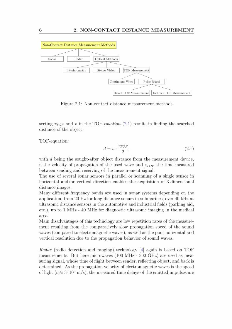
The measurement of distances is essential for many technical applications. Theclassical direct distance measurement, which means the direct comparison ofthe distance with a calibrated ruler, is the oldest and most obvious method,but not applicable in many cases. Therefore various indirect distance measure-ment procedures were developed throughout the centuries; here the distance isderived of any distance depending measure which is easier to access than thedistance itself. The most important subgroup of the indirect distance measure-ment is the non-contact distance measurement, as many technical applicationsrequire distance measurement without any physical contact between the dis-tance meter and the measured object. Therefore, up from the beginning ofthe 20th century measurement procedures using sound waves and electromag-netic waves to transfer the distance information to the measuring instrumenthave been developed. Figure 2.1 gives an overview of todays most commonnon-contact distance measuring methods, which are closer described in thefollowing sections.
2.1 Sonar and Radar
Sonar (sound navigation and ranging) systems derive the distance betweenthe sonar device and an object via time of flight (TOF) measurement [3]. Asdepicted in figure 2.2, a sonic measuring impulse is emitted by the sender andpropagates through the supporting medium (air, water, etc.) with the accord-ing propagation speed v. If the sound waves meet objects on their course ofpropagation, the waves are partly reflected back. This reflections can be de-tected by the sender/receiver device, what enables a measurement of the timeτTOF elapsed between the sending and the receiving of the sound impulse. In-
6 2. NON-CONTACT DISTANCE MEASUREMENT
Indirect TOF Measurement
Pulse BasedContinuous Wave
Interferometry Stereo Vision
RadarSonar Optical Methods
TOF Measurement
Direct TOF Measurement
Non-Contact Distance Measurement Methods
Figure 2.1: Non-contact distance measurement methods
serting τTOF and v in the TOF-equation (2.1) results in finding the searcheddistance of the object.
TOF-equation:
d = v · τTOF
2, (2.1)
with d being the sought-after object distance from the measurement device,v the velocity of propagation of the used wave and τTOF the time measuredbetween sending and receiving of the measurement signal.The use of several sonar sensors in parallel or scanning of a single sensor inhorizontal and/or vertical direction enables the acquisition of 3-dimensionaldistance images.Many different frequency bands are used in sonar systems depending on theapplication, from 20 Hz for long distance sonars in submarines, over 40 kHz atultrasonic distance sensors in the automotive and industrial fields (parking aid,etc.), up to 1 MHz - 40 MHz for diagnostic ultrasonic imaging in the medicalarea.Main disadvantages of this technology are low repetition rates of the measure-ment resulting from the comparatively slow propagation speed of the soundwaves (compared to electromagnetic waves), as well as the poor horizontal andvertical resolution due to the propagation behavior of sound waves.
Radar (radio detection and ranging) technology [4] again is based on TOFmeasurements. But here microwaves (100 MHz - 300 GHz) are used as mea-suring signal, whose time of flight between sender, reflecting object, and back isdetermined. As the propagation velocity of electromagnetic waves is the speedof light (c ≈ 3 ·108 m/s), the measured time delays of the emitted impulses are

2.2 Optical Distance Measurement Techniques 7
Sended wave
Reflected wave
Distance d
Sen
der
/R
ecei
ver R
eflectin
gob
ject
Figure 2.2: Principle of time of flight measurements
very short (6.67 ns/m). This necessitates very accurate evaluation electronics,but on the other hand results in very fast measurement repetition rates. Hencescanning procedures for 2D or 3D radar imaging are made feasible. Besidesthe distance information, a radar system can also determine the velocity of atarget by evaluating the Doppler shift of the signal; this is e.g. used for trafficspeed control.Radar distance measurement is used for a variety of applications over a hugerange of different distances. Examples are distance measurement for automaticcruise control in automobiles (up to 200 m), air traffic surveillance (distancerange up to 500 km), or the mapping of planets in our solar system.But also radar systems suffer from their poor angular resolution properties.Complex antennas can lower this problem, but this again leads to bulky sys-tems which are not practicable for many applications.
2.2 Optical Distance Measurement Techniques
Non-contact distance measurement methods based on light waves are commontechniques for many different distance measuring applications. In the followingthe most important ones are introduced:
2.2.1 Interferometry
Interferometry is a very precise technique to measure distance [5] indirectlyfrom a phase shift of light waves. Figure 2.3 shows the Michelson interferom-eter to make clear the measuring principle.
A laser source emits a coherent laser beam of a fixed frequency f onto asemipermeable mirror that divides the beam into two parts. The first part isdeflected towards a reference target with calibrated distance, and is then partly

8 2. NON-CONTACT DISTANCE MEASUREMENT
lasersou
rce
receiver
mea
sure
dob
ject
semipermeable mirror
reference target
Figure 2.3: Michelson interferometer
reflected into the detector from there. The second part passes the semiperme-able mirror and illuminates a point on the measurement target. Parts of theincident light are reflected from there towards the detector over the semiper-meable mirror. In the detector the portions from the reference target and themeasurement target interfere with each other to a resulting signal. By movingthe beam splitter mirror a detector amplitude characteristics is derived whichcontains the relative distance information for the measured target point in itsphase. By evaluating the phase shift ∆φ of this signal, the relative distancecan be determined as
∆d = c · ∆τTOF
2= c · ∆φ
4 · π· 1
f. (2.2)
With up to λ/100 the achievable distance resolution is in the range of a few nm,but unambiguous measurements are only possible within a distance range ofa half λ. This is no problem at relative distance measurements for i.e. surfacescanning, but makes absolute distance measurements impossible. To solve thisproblem techniques like using several wave lengths are known.
2.2.2 Triangulation
As 2D imaging does not provide depth information of a captured scene, tri-angulation is used to generate 3D image data of a scene using standard 2D

2.2 Optical Distance Measurement Techniques 9
imaging systems. The idea is thereby the observation of a scene from twodifferent camera positions, i.e. under different observation angles. On this ba-sis different techniques are known to get 3D data; here stereo vision (section2.2.2.1) and active triangulation (section 2.2.2.2), two very common triangu-lation variants, are introduced.
2.2.2.1 Stereo Vision
Stereo vision [5] uses two cameras that observe a scene from two different po-sitions, as depicted in figure 2.4a (intersection through a 3D scene). Thus theoptical centers of the two cameras and the observed object point P form atriangle, whose basis length b and the two angles α and β are known. Con-sequently all other quantities, including the height d – the searched objectdistance – can be calculated. This is done by means of the so-called ’dispar-ity’, which contains the distance information of the object point P . Equations2.3 - 2.6 show the derivation of the disparity p.
������������������������������������
b, active triangulation
measured object
d
f f
projector camera
x2
α β
b
camera 1 camera 2
x1 x2
α β
b
a, stereo vision
measured object
d
y y
Figure 2.4: Principles of stereo vision and active triangulation

10 2. NON-CONTACT DISTANCE MEASUREMENT
p = x1 − x2 (2.3)
= f · tan(α)− f · tan(β) (2.4)
= f · y + b/2
d− f · y − b/2
d(2.5)
= b · fd
(2.6)
Resolving equation 2.6 for d and inserting equation 2.3 leads to following simpleformula for the calculation of the distance d of object point P :
d =b · fp
=b · f
x1 − x2
, (2.7)
with x1 and x2 being the position of the image of object point P on the imagingsensor of camera 1 and camera 2 respectively.
A disadvantage of the stereo vision method is the need of separating the twocameras. The larger the distance range is, the longer the required basis widthb becomes, in order to keep the measurement error in a reasonable range (cf.equation 2.8).
∆d =b · fp2
·∆p =d2
b · f·∆p (2.8)
This is applicable for static measurements, but not for mobile systems. Alsothe necessity of having high contrast in the scene surfaces for the identificationof identical points in the two pictures is often not tolerable. Further shadingproblems can occur; for scene points that are visible for only one camera, nodistance value can be calculated.Applications for stereo vision are for example 3D vision for robot systems andworkpiece scanning in automated production lines.
2.2.2.2 Active Triangulation / CCT
Contrary to stereo vision, active triangulation [5] uses only one camera and alight source instead of the second camera. This light source projects a lightpattern onto the observed scene which is imaged on the image sensor of thecamera (see figure 2.4b). Thus again a triangle is formed, here between thelight source, the object point and the camera. For calculation of the distance ofa scene point, the knowledge, from which direction the point was illuminated(angle α in figure 2.4b), is required. Using a repeating pattern of different

2.2 Optical Distance Measurement Techniques 11
intensities for different illumination angles, the sensor can decode this infor-mation and re-calculate the angles. But the repetition of the pattern leads toan ambiguity problem, which can severely affect the resulting 3D image, espe-cially for scenes containing complex depth information. This can be avoidedby combining several measurement steps using light patterns with differentspatial frequencies; this on the other side is a time consuming procedure. Amore advanced and effective method is the so-called color coded triangulation(CCT) [6], which uses an unambiguously coded pattern of light stripes of dif-ferent colors for scene illumination.
For active triangulation the formula to calculate the distance value of point Pis
d =b · fp
=b · f
f · tan(α)− x2
, (2.9)
with α being the angle of the light beam illuminating object point P and x2
being the position of the image of object point P on the imaging sensor of thecamera.
Disadvantage of the active triangulation method is, besides the basis width andshading problems described in 2.2.2.1, the presence of the scene illuminationpattern, which is disturbing in many applications, specially if humans are partof the observed scene. Newest systems solve this problem using illuminationin the infrared spectrum, invisible to the human eye [7].Another problem of this approach is the sensitivity towards ambient light. Thismeans that measurements can severely be disturbed, if light from outside thecamera system outshines the projectors light pattern. Bandpass filtering ofthe incident light according to the illumination wavelength is possible to lowerthat influence.3D face recognition for security applications as well as 3D measuring tasksfor industrial application are only two of many possible applications for CCTsystems.
2.2.3 Time of Flight Distance Measurement
According to the TOF distance measurement by usage of sound waves or mi-crowaves (cf. chapter 2.1), several TOF distance measurement procedures usinglight waves are known. They all actively emit light in order to derive the dis-tance of a reflecting object by measuring the time which the light needs topropagate to the object and return to the combined emitter/sensor device.The different approaches are described in the following paragraphs:

12 2. NON-CONTACT DISTANCE MEASUREMENT
2.2.3.1 Continuous Wave Methods
B
Emitted
Received
light
light
Gatedphotodetectors
D = A−B
A
A B A B A B A B
Exposure time
1/fL
τTOF
t
t
t
on gate ATotal light
on gate BTotal light
Bias
1/fL
tTOF
Figure 2.5: Principle of continuous wave time of flight distance measurementaccording to [8]
Continuous wave (CW) distance measuring systems [8,9,10] derive the desireddistance information from the phase shift of an emitted light pulse sequence.For this purpose usually IR LEDs are modulated with a modulation frequencyfL (typically in the range of 5 MHz to 100 MHz) with a duty cycle of 50%.Synchronized with the emitted light, photodetectors A and B are alternatelygated during the exposure time that is usually 1 ms to 50 ms (see figure 2.5).Thus the phase shift of the received signal due to the time of flight τTOF directlyinfluences the amount of photocharges at the outputs of A and B (lower partof figure 2.5). A difference signal D = A − B is calculated for cancelling ofbiases. For the derivation of the phase φ a second observation of D with thetiming of the gated photodetectors A and B shifted by 90◦ is conducted. Phaseφ can then be calculated according to equation 2.10 as
φ = tan−1
(D90
D0
). (2.10)
Following the object distance can be found as
d = c · τTOF
2= c · TPW · φ
4 · π. (2.11)

2.2 Optical Distance Measurement Techniques 13
A weak point of the continuous wave methods are ambiguity problems, i.e.the range of uniqueness is limited to phase shifts of 0 ≤ φ ≤ π. The distanceof objects causing a higher phase shift is hence misinterpreted. As solutionalgorithms combining several different modulation frequencies are used; this forsure is a more time-consuming procedure, resulting in lower image repetitionrates. Also the sensibility towards ambient light due to the comparatively longintegration duration is a problem for CW distance measurement systems; itcauses pixel saturation that makes a distance measurement impossible. Mucheffort with respect to background light suppression – like filtering the incominglight, resetting photodector bias for A andB several times during exposure, etc.– were taken to make these systems competitive in view of outdoor applications[8, 11].
2.2.3.2 Pulse Based Methods
In contrast to the CW methods, the pulse based distance measurement proce-dures utilize the time of flight of single light pulses to determine the distanceof objects. Thereby one distinguishes between two different approaches, the’direct’ and the ’indirect’ pulse based TOF measurement.
2.2.3.2.1 Direct TOF Measurement
The direct pulse based TOF measurement physically measures the time offlight of an emitted laser pulse. I.e., at the emission of a short light pulse ahigh-speed counter is started, which is stopped when the return of a reflectionof the pulse was detected in the detector device [12]. The distance of thereflecting object is then given as
d = c · τTOF
2. (2.12)
Due to the complexity of the detection and evaluation electronics, a paralleliza-tion in a high-resolution sensor array is not feasible at the present time. Hencethe available systems either provide only a few measurement points like thelidar-systems (light detection and ranging) [13] or apply scanning techniquesby means of rotating mirrors, to measure one scene point after the other (laserscanners [14]).
2.2.3.2.2 Indirect TOF Measurement (3D-CMOS)
Here the time of flight of the emitted light pulse is not measured directly but viaaccumulation of charges on a sensor chip from which the distance information

14 2. NON-CONTACT DISTANCE MEASUREMENT
can be calculated. Thus the procedure is equal to the CW method from chapter2.2.3.1 using only a very short single light pulse (typically 20 ns - 200 ns)instead of a pulse sequence. For the derivation of τTOF several procedures areknown [15, 16]. Concept is always based on the use of imaging pixels withextremely short exposure times in the range of the laser pulse length, whichare capable to produce TOF-dependent signals. The object distance d is thencalculated with the TOF-equation (2.1). In this thesis the so-called 3D-CMOSsensor, which performs indirect pulse based TOF distance measurement, andits distance derivation algorithms are addressed. See chapters 3 and 4 for aclose description of these topics.

Chapter 3
Theory of DistanceMeasurement with 3D-CMOSSensor
3.1 Measuring Principle
Algorithm
MeasurementPulsed
DataDistance
Illumination
3D-CMOSArray
Distance
Figure 3.1: 3D-CMOS measuring principle
The 3D-CMOS sensor system performs a pulse based indirect TOF measure-ment using near infrared (NIR) laser pulses in the range of 20 ns - 200 ns.As figure 3.1 shows, these pulses are sent by the internal illumination mod-ule of the camera; after diffuse reflection by the observed scene objects theyreturn temporally delayed and with reduced amplitude to the camera device.The camera lens passes a part of the backscattered light and thus images theobserved scene onto the surface of the 3D-CMOS sensor chip. The chip (cf.

16 3. THEORY OF 3D-CMOS DISTANCE MEASUREMENT
chapter 4.1.1) contains light sensitive pixels which are operated as electronicshort-time windowed integrators synchronized to the emitted laser pulse forTOF dependent collection of charges generated by the incident light. Differentevaluation algorithms have been developed (chapter 3.4) to derive the pulsedelay τTOF from a specific number of single measurements. This leads to theobject distance
d = c · τTOF
2. (3.1)
3.2 Camera Optics
A lens camera model is used for all considerations in this thesis, as shown infigure 3.2. The camera optics is thereby defined by an imaging lens of focallength f , a sensor plane parallel to the lens plane and an aperture limiting theeffective diameter of the lens to D. Its optical axis is defined as the straightline through the optical center O that is perpendicular to the sensor plane.
Sensor plane
f
Lens plane
PyP
u v
P ′
Foptical axis
O
yP ′ D
Focal plane
Figure 3.2: Imaging geometry
The mapping of a point P in the object space to the image space is describedby the lens law [17]:
1
f=
1
u+
1
v(3.2)
with u and v being the distances of P and P ′ normal to the lens plane, respec-tively.
Actually, for each object distance u an unique image distance v exists, at whichthe sensor has to be positioned at to obtain a sharp image P ′ of P . But here

3.3 Signal Generation 17
we assume large object distances compared to the focal length (u � f), sothat v can be approximated as
v =1(
1f− 1
u
) ≈ f with u� f . (3.3)
With equation 3.3 the magnification M of the image in relation to the objectis defined as
M =v
u=f
u, (3.4)
what leads to equation 3.5, describing the perspective projection of objects onthe sensor plane:
yP ′ = −yP ·M = −yP ·f
u(3.5)
A further key parameter of the camera lens is the f-number f#, which is theratio of the focal length f to the aperture diameter D:
f# =f
D(3.6)
It is a measure for the photo-sensitivity of the camera optics, but also influ-ences the imaging properties [17].
In the following considerations effects like chromatic or spherical aberrations orblurring due to the the approximation taken in equation 3.3 are not included.Their influence on the imaging properties of the camera is assumed as negligiblein this thesis. Justification for this assumption will be given in chapter 4.2.1.4.
3.3 Signal Generation
This section deals theoretically with the generation of signals with inherentdistance information using the 3D-CMOS camera. I.e., ideal signal shapes(e.g. a rectangular impulse is assumed to model a laser light impulse; in realitya laser pulse certainly has finite leading and trailing edges) and ideal signalprocessing operations are applied to model the processes during the distanceacquisition procedure. To what extent these idealizations are justified, andwhich adaptations have to be done in practice will be discussed in chapter 4.
3.3.1 Pulsed Illumination
The scene illumination module of the 3D-CMOS sensor generates pulses witha pulse width in the range of some tens to hundreds of nanoseconds. Here the

18 3. THEORY OF 3D-CMOS DISTANCE MEASUREMENT
pulses are assumed to be ideal rectangular pulses according to equation A.2in appendix A.1 with amplitude PL and pulse width TPw. See equation 3.7as well as figure 3.3 for the laser modules radiant power characteristics for asingle laser pulse.
PLaser(t) = PL · rect(t− 1
2· TPw − TDL
TPw
). (3.7)
0
PL
TDL TDL + TPw
TPw
t
PLaser(t)
Figure 3.3: Ideal laser-pulse function
The shift by 12·TPw towards positive t-direction is introduced to make the pulse
start at t = 0 s, the additional shift by TDL denotes an purposely inserted delayof the laser pulse by means of a delay component on the camera hardware (seechapter 4.1.4). This feature is used by some of the later examined distancederivation algorithms.
3.3.2 Reflected Signal
According to figure 3.1 the laser pulse is sent towards the scene, the distanceof which is to be determined. Following boundary conditions are postulatedregarding the illumination:
• The whole emitted radiant power illuminates an area AObject in the objectspace, image of which in the image space corresponds to the active sensorarea ASensor; i.e. no light power is lost by illuminating those parts of thescene that are not imaged onto the sensor
• The radiant power is homogeneously distributed over the area AObject
• The laser source and the sensor chip are positioned close together; thusthey can be assumed as being located at the same point

3.3 Signal Generation 19
The delay of the laser light due to the distance d between camera and object(TOF) amounts to
τTOF =2 · dc
, (3.8)
so that the irradiance on the sensor surface is given by
ESensor(t, τTOF , α) =PLaser(t− τTOF )
AObject
· ρ · κ · cos4(α) · 1
4 · f 2#
, (3.9)
with
PLaser(t− τTOF ) radiant power of the laser module shifted by τTOF
α angle between optical axes and camera rayAObject irradiated object areaρ object surface reflectivityκ optical loss factor of camera and laser module opticsf# f-number according to equation 3.6.
The cos4 dependency on the viewing direction α is closely investigated in [18].For the following theoretical considerations α is assumed as 0, i.e. the objectarea close the the optical axis is considered.
Substituting
AObject = ASensor ·(d
f
)2
(3.10)
in equation 3.9, ESensor(t, τTOF , α) can be calculated as
ESensor(t, τTOF , α = 0) = ESensor(t, τTOF ) =PLaser(t− τTOF )
ASensor
·ρ ·κ · f 2
4 · f 2# · d2
.
(3.11)
For the following parts of this chapter the amplitude of the received laser lightirradiance ESensor(t) on the sensor surface is assumed as being independentfrom the object distance d and the object reflectivity ρ for reasons of trans-parency of the line of argument. Though this assumption does not correspondto the reality situation, it does not falsify the considerations.
3.3.3 Short Time Integration
The 3D-CMOS sensor chip implements short-time windowed integration of thephotocharge generated by the illumination of the sensor surface. The duration

20 3. THEORY OF 3D-CMOS DISTANCE MEASUREMENT
of these so-called shutter windows is in the range of the laser pulse duration,i.e. in the nanosecond range (cf. section 4.2.1.2). The shutter windows can bedescribed as rectangular windows (see annex A.1) of the sensitivity value ofthe sensor (figure 3.4), which relates the pixel diode current to the incidentradiant power. It is thus measured in A/W. Whilst the sensitivity is zero inthe normal case, it becomes SλS during the integration time TInt. For a givenwavelength λ the sensitivity thus results as
SλSensor(t) = SλS · rect(t− 1
2· TInt − TDS
TInt
). (3.12)
where TDS is an additional shift of the shutter window introduced for later useduring distance measurement.
0
t
TInt
TDS TDS + TInt
SλSensor(t)
SλS
Figure 3.4: Ideal sensor sensitivity function
3.3.4 Integrator Output Signal
The incident light reflected by an observed scene generates a diode currentID(t, τTOF ) in the light sensitive sensor pixels as described by following equa-tion:
ID(t, τTOF ) = SλSensor(t) · ESensor(t, τTOF ) · APixel (3.13)
The integration of ID(t, τTOF ) at the integration capacitance CInt (which con-sists of the diode inherent capacitance CD plus the sense capacitance Csense
as one can see in figure 4.3) during the integration time TInt generates anintegrator voltage UInt in the considered pixel:
UInt(τTOF = τ1) =Qphoto(τTOF = τ1)
CInt
=
∞∫−∞
ID(t, τTOF = τ1)dt
CInt
(3.14)

3.4 Distance Derivation Algorithms 21
Doing this calculation for all possible values of τTOF results in a function thatdescribes the integrator output voltage in dependence on the time of flightof the laser pulse, i.e. in dependence on the object distance. The qualitativecharacteristics of UInt(τTOF ) for given times TPw and TInt can be seen in figure3.5; note that irradiance variations due to object distance and reflectivity are– as already mentioned in section 3.3.2 – not considered here.
UInt(τTOF ) =
∞∫−∞
ID(t, τTOF )dt
CInt
(3.15)
=
∞∫−∞
SλSensor(t) · ESensor(t, τTOF ) · APixeldt
CInt
(3.16)
=Qphoto(τTOF )
CInt
(3.17)
UInt(τTOF )
0 TInt − TPw TInt−TPw
TDL − TDS + τTOF
Figure 3.5: Ideal integrator output function for variation of the laser pulsedelay
Over readout circuitry (cf. chapter 4.1.1.1) the integrator output voltage UInt
is transferred to the output buffer of the image sensor and is then available forfurther processing as sensor output signal.
3.4 Distance Derivation Algorithms
Using the sensor output signals derived in the previous section, the derivationof an object distance to be measured from them is the first goal of the furtherprocessing steps. For this several distance derivation algorithms exist; basicidea of all of them is the recovery of the distance information from reflectedpulses by using short-time shutter windows that overlap the incident light pulse

22 3. THEORY OF 3D-CMOS DISTANCE MEASUREMENT
depending on the delay τTOF . Four elementary relative positions between theincident pulse and the shutter window can be distinguished, as shown in figure3.6:
a) The overlap decreases with increasing τTOF ; the pulse ’moves out’ of theshutter window for increasing distances.
b) The overlap increases with increasing τTOF ; the pulse ’moves into’ theshutter window for increasing distances.
c) Due to the long duration of the shutter window τTOF has no influence onthe overlap and thus no influence on the sensor signal. The sensor signalis a measure for the pulse overall radiant energy. The use will becomeclear in the next chapter.
d) This kind of shutter window to pulse arrangement gives an signal partlyindependent of τTOF (as long as it is fully ’filled’ by the pulse) and partlydependent on τTOF . In practice it is not used. It will thus not be takeninto account in the later details.
The lower part of figure 3.6 shows the sensor output signals Ua(τTOF ) toUd(τTOF ) for the above shutter window and pulse alignments with respectto the laser impulse delay τTOF . These signals are the basis for the calculationof the object distance one is searching for.The following sections introduce all feasible distance acquisition algorithmswithout further addressing of performance behavior or other features. Aninvestigation toward those issues will be given in chapter 5.
3.4.1 MDSI
The MDSI (multiple double short-time integration) algorithms yield the dis-tance information from two single sensor signals (from the set of a), b) or c) infigure 3.6), as the word ’double’ in the name implies. The meaning of ’multi-ple’ will be explained later in section 4.1.1.3. Four reasonable combinations oftwo of these sensor signals are possible in order to obtain the distance of themeasured object, consequently four MDSI variants exist:
MDSI1MDSI1 extracts the necessary information from one shutter of category a), andone of category c). Although the first shutter operation generates distanceinformation in the output signal Ua(τTOF ), the searched distance d can notbe retrieved directly, as the sensor output signal is also influenced by the

3.4 Distance Derivation Algorithms 23
Shutter alignment b)
Shutter alignment c)
Shutter alignment d)
τTOF
τTOF
τTOF
τTOF
Shutter alignment a)
Shutter alignment b)
Shutter alignment c)
Shutter alignment d)
Ua(τTOF )
Ub(τTOF )
Uc(τTOF )
Ud(τTOF )
Received laser pulse
t
t
t
t
t
TPw
TInt
TInt
TInt
TPw
τTOF TPw
t
Sensor output signals:
TPw
Temporal laser pulse and shutter window alignment:
ESensor(t)
PLaser(t)
SλSensor(t)
SλSensor(t)
SλSensor(t)
SλSensor(t)
Emitted laser pulse
TInt
Shutter alignment a)
Figure 3.6: Possible alignments of a shutter window relatively to the incidentlight pulse

24 3. THEORY OF 3D-CMOS DISTANCE MEASUREMENT
irrandiance value of the reflected light pulse. By normalizing the signal withthe pulse overall irradiance value, which is measured by a shutter windowoperation of the type c), the distance can be calculated using the MDSI1equation stated below:
d =c
2·(TPw − TPw ·
Ua
Uc
− (TDL − TDS)
)(3.18)
where TPw, TDL and TDS denote the width and the relative temporal positionof the according laser pulses and shutter windows as described in sections 3.3.1and 3.3.3.
MDSI2The MDSI2 procedure is quite similar to MDSI1. Solely a type b) instead ofthe type a) shutter window is applied. Thus the distance calculation equationchanges to
d =c
2·(TPw ·
Ub
Uc
− (TDL − TDS)
). (3.19)
MDSI3Here the long shutter window of type c) is substituted by the sum of two shortshutter windows of type a) and b) for the distance calculation. This is possible,because the sum signal of a) and b) (cf. figure 3.6) equals the sensor outputof c).
d =c
2·(TPw − TPw ·
Ua
Ua + Ub
− (TDL − TDS)
)(3.20)
MDSI4MDSI4 corresponds to MDSI3 unless a class b) shutter window instead of classa) is used in the enumerator of the fraction term in the d-equation:
d =c
2·(TPw ·
Ub
Ua + Ub
− (TDL − TDS)
)(3.21)
All these algorithms deliver the identical results of the measured object dis-tance. The measurement range is for all limited to
0 ≤ d ≤ c · TPw
2. (3.22)

3.4 Distance Derivation Algorithms 25
3.4.2 Gradient Method
Contrary to the MDSI algorithms, this method does not process a TOF de-pendent signal, which is normalized by a second ,TOF independent, signal,but two TOF dependent shutter windows are used. Their temporal alignmentis depicted in figure 3.7. Basic principle is the use of the temporal difference∆TInt between the two shutter windows. The distance of the pulse reflectingobject can be calculated by employing equation 3.23 below.
t
t
t
TPw
Sensor output signals:
τTOF,max
∆TInt
TPw
τTOF
Shutter alignment a1)
Ua1(τTOF )
Ua2(τTOF )
TInt,a2
TInt,a1
TInt,a1
TInt,a2
Shutter alignment a2)
PLaser(t)
SλSensor(t)
SλSensor(t)
Emitted laser pulse
Temporal laser pulse and shutter window alignment for the gradient method:
Figure 3.7: Alignment of a shutter window relatively to the incident light pulseat the gradient method
d =c
2·(TInt,a1 − (TInt,a1 − TInt,a2) ·
Ua1
Ua1 − Ua2
)=
c
2·(TInt,a1 −∆TInt ·
Ua1
Ua1 − Ua2
)(3.23)
Here also a variation of the method is possible with respect to the use of shutterwindows of type b), i.e. the overlap of shutter window and reflected pulse isrising for increasing values of τTOF . The resulting equation slightly changes to

26 3. THEORY OF 3D-CMOS DISTANCE MEASUREMENT
d =c
2·(TInt,b1 −∆TInt ·
Ub1
Ub1 − Ub2
). (3.24)
3.4.3 CSI and DCSI
The correlated short-time integration (CSI) and difference correlated short-timeintegration (DCSI) procedures differ from the previous distance calculationmethods as they utilize a sequence of shutter measurements instead of twosingle measurements one range acquisition.
CSIIn this method a sequence of shutter windows is applied to a sequence of equalshaped light pulses, whose trigger position compared to the shutter window isshifted by known delays TDL,1, TDL,2, etc. (cf. the schematic illustration figure3.8). Reasonable is the usage of a shutter window width in the range of thelight pulse width. Depending on the light pulse shift TDL the intensity charac-teristics U(TDL) can be derived (see lower part of fig. 3.8). Determination ofthe TDL-value TDL(U(TDL)max), where the curve reaches its maximum, leadsto the object distance by inserting into equation 3.25:
d =c
2· (TDS − TDL(U(TDL)max)) (3.25)
Though this procedure seems to be suitable for TOF distance measurement, itsperformance turned out to be inferior when compared to the other proceduresintroduced here [19]. Main disadvantage is the susceptibility to systematicerrors at the determination of TDL(U(TDL)max) that makes the procedure un-feasible. Thus it is only mentioned here for the sake of completeness and willnot be considered in further examinations.
DCSI
The DCSI distance derivation method is an advancement of the CSI methodpresented above. Two shutter signal sequences according to CSI are appliedhere with two shutter windows 1 and 2, that are temporally arranged as one cansee in figure 3.9. The resulting output signal characteristics U2(TDL) of shutter2 is then subtracted from U1(TDL) of shutter 1; this leads to the difference signalU(TDL) = U1(TDL)− U2(TDL) shown in green color in figure 3.9. For distancecalculation the TDL-value of the zero-crossing TDL(U(TDL) = 0) = TDL0 of themedium part of the difference curve has to evaluated. Inserting this value intoformula 3.26 yields the searched distance value.

3.4 Distance Derivation Algorithms 27
Sensor output signals:
Temporal laser pulse and shutter window alignment at CSI:
TDL
t
t
t
Shutter alignment
Received laser pulses
with increasing TDL
TDL,2
TDS − τTOF
U(TDL)
TDS
τTOF
TPw
TDL,1PLaser(t)
ESensor(t)
SλSensor(t)
Emitted laser pulses
Figure 3.8: Example for the temporal alignment of laser pulses and shutterwindows at the CSI method
d =c
2·(TDS,1 − TDS,2
2− TDL(U(TDL) = 0)
)=
c
2·(TDS,1 − TDS,2
2− TDL0
)(3.26)
The subtraction of the shutter signal curves brings many advantages com-pared to CSI, as elimination of potential systematic influences like offsets ornonlinearities of the shutter windows and the laser pulse; additionally thedetermination of the the time of flight becomes a line fitting through the mea-sured TDL-curve points for derivation of the zero crossing. See annex C for amathematical description of this procedure.
3.4.4 Conclusion
All of the above distance measuring methods are suited to derive the distanceof an scene object to be measured from an according set of sensor outputs. It isimportant that in all equations 3.18-3.26 any dependence on parameters PLaser,AObject, ρ, κ, α, and f# has been eliminated. This is valid, however, only ifnone of these parameters has changed during the shutter window operationsbelonging to the same distance calculation equation.

28 3. THEORY OF 3D-CMOS DISTANCE MEASUREMENT
1 2
Emitted laser pulses
PLaser(t)
SλSensor(t)
Sensor output signals:
t
t
t
Shutter alignment
Received laser pulses
with increasing TDL
TDL,2
τTOF
TPw
TDL,1
Temporal laser pulse and shutter window alignment at DCSI:
TDL
U1(TDL)U2(TDL)
TDL
TDS,1
TDS,2
U1(TDL)− U2(TDL)
ESensor(t)
TDS,1+TDS,2
2− τTOF
Figure 3.9: Distance measurement principle of the DCSI method
Differences between the methods are the reachable measurement accuracy aswell as the applicability for the proposed sensor applications (cf. chapter 1).Chapter 5 introduces investigations regarding those issues.

Chapter 4
3D-CMOS Array Sensor System
b
a
d
c
b
Figure 4.1: 3D-CMOS array sensor system
This chapter describes the 3D-CMOS array sensor system examined in thisthesis and its performance characterization [20, 21]. As depicted in figure 4.1,the main components of the system are:
a) Electronics boards including the array sensor chip
b) Laser illumination modules
c) Imaging optics
d) Power supply

30 4. 3D-CMOS ARRAY SENSOR SYSTEM
The following sections give a close description of the components and theconducted experiments.
4.1 System Components
4.1.1 Novel Array Sensor
The novel 64x8 pixel 3D-CMOS array sensor is the main component of thesensor system. It was developed by the Fraunhofer IMS within the UseRCamsproject on the basis of an existing 64x4 pixel 3D-CMOS sensor chip [22, 23].Its functionality allows the indirect measurement of the time of flight of laserpulses in the ns-range.Figure 4.2 shows the photograph of the sensor chip realized with a 0.5 µmn-well CMOS process. It includes 64·8 = 512 photo diode pixels, a suitablereadout circuit per half-column including a CDS stage with analog accumula-tion capability (see sections 4.1.1.2 and 4.1.1.3), multiplexers for selecting therows, as well as an analogue buffer circuit for each output channel (total 2).The light sensitive pixel area can be seen in the center of the chip. The pixelpitch is 130 µm in horizontal and 300 µm in vertical direction; this results in asensitive area of 64·130 µm · 8·300 µm = 19.97 mm2. As the whole peripheralpixel electronics is placed in the upper and lower areas of the chip, the activepixel areas join each other directly, i.e. the fill factor (FF ) of the active pixelarea is nearly 100 %.
4.1.1.1 Pixel Structure
The circuit diagram of the pixel circuit used in the 64x8 pixel 3D-CMOS arraysensor is shown in figure 4.3 [23]. Each pixel circuit contains a reverse biasedn-well/p-substrate photo-diode PD with a inherent capacitance CD (5.1 pF),a reset switch (Φ1), a shutter switch (Φ7x), a sense capacitor Csense (1 pF),a buffer SF (amplification factor gSF = 0.85), a hold capacitor CH , and aselect switch (Φ2x). Each four pixel circuits located in one half-column alwaysshare a single readout switched-capacitor amplifier which also performs thecorrelated double sampling (CDS) operation (see section 4.1.1.2). This quad-to-single multiplex reduces considerably the hardware complexity.Note that in the following the pixel index (0-3), as it is sometimes used in figure4.3, is not considered, because the pixels of one row are absolutely identical.Φ70 for example is denoted as Φ7 and so on.The circuit operation relies on a periodical reset of the photo-diode capaci-tance CD and the sense capacitance Csense to a fixed reference voltage (Uddpix)and subsequent discharge due to the photo-current. The shutter switch (Φ7)

4.1 System Components 31
Figure 4.2: 64x8 pixel 3D CMOS sensor
controls the integration time of the discharge process, as depicted in figure 4.4.Then the remaining voltage stored at Csense is read out into a second capacitorbank CH acting as a hold capacitor. The charges held at CH are read out us-ing the correlated double sampling (CDS) stage by activating the select switchΦ2. Meanwhile, the acquisition of the next value on Csense is performed, thusthis architecture yields quasi-continuous light acquisition with minimum deadtime.After a signal acquisition cycle the pixel output signal after the CDS stage ispresent as USensor,raw on the sensor output. Given a sensor irradiance profileESensor(t) and a shutter window function SλSensor(t), this voltage is given as
USensor,raw = Uref4 −Qphoto
CD + Csense
· gSF ·CCl
CF
, (4.1)
where
QphotoEq. 3.16
= APixel ·+∞∫0
SλSensor(t) · ESensor(t)dt . (4.2)
Note that this equation differs from equation 3.14 due to presence of resetvoltage Uref4, the sign inversion, and the signal amplification factor gSF · CCl
CF
(gSF = 0.85, CCl = 10 pF, CF = 2.5 pF), because equation 4.1 reflects the realhardware implementation including the pixel readout circuitry.

32 4. 3D-CMOS ARRAY SENSOR SYSTEM
+
−
Φ
Φ
ΦΦ
Φ
Φ
Φ
Φ
Φ
Φ
Φ
Φ
Φ
Φ
Φ8
Φ
Φ8
↓ USensor,raw
Figure 4.3: Pixel circuit with CDS readout stage [23]
measurement of laser pulse + background irradiance
Received laser pulseESensor(t)
TPwTReset
Φ1(t)
UInt(t) Integrator voltage
measurement of background irradiance
Emitted laser pulsePLaser(t)
τTOF
τTOF
ON
TPwTReset
OFF
Shutter signalΦ7(t)
Reset signal
Figure 4.4: Simplified sensor timing [22]

4.1 System Components 33
Preprocessing of the sensor data in the system internal FPGA removes Uref4
of USensor,raw and inverts its sign. The result is the simplified sensor outputvoltage USensor
USensor =Qphoto
CD + Csense
· gSF ·CCl
CF
, (4.3)
which is used as sensor output signal in all further considerations.
4.1.1.2 Correlated Double Sampling
The amount of light received from an object not only depends on the emittedlaser power PLaser(t), the reflectance ρ of the object and its distance, but alsoon the amount of EBack(t) due to the incident light of other light sources.The influence of EBack(t) is eliminated by measuring solely the backgroundirradiance without laser pulse, i.e. PLaser = 0, and subtraction of this valuefrom the measurement with laser pulse. Thus each measurement must beperformed with laser pulse ON and OFF (cf. figure 4.4) and the differencebeing stored on the corresponding capacitance CF in the analog memory. Thewhole procedure
1: Usense|ON ∝ ESensor(t) + EBack(t) (4.4)
2: Usense|OFF ∝ EBack(t) (4.5)
1 − 2:CDS=⇒ USensor ∝ ESensor(t) (4.6)
results in a pixel output signal that is independent of EBack(t) if the twomeasured values of EBack are correlated. This assumption is valid, if EBack doesnot change within the CDS cycle period, what is always granted in normalenvironments. The corresponding control signals of the sensor are shown infigure 4.4. Note that we do not have to carry out an additional reset samplingin this case, we simply measure with the laser ON and OFF and subtract themeasurements.
4.1.1.3 Analog Accumulation and Adaptive Accumulation
A unique feature of the 3D-CMOS image chip is the analogue real-time on-chip accumulation process at each individual pixel using multiple pulses foreach shutter window [15]. By this means the signal-to-noise ratio increasesand leads to an improved distance accuracy. Repetitive accumulation of nacc
laser pulses (cf. figure 4.5) is performed adaptively up to the saturation levelat each pixel element. Intelligent procedures can be employed to cover a large

34 4. 3D-CMOS ARRAY SENSOR SYSTEM
range of target distances and target surface reflectivities with this adaptivepulse illumination method (see section 4.2.3.3).
1 2 3 4
PLaser(t)
ESensor(t)
SλSensor(t)
t
tReceived laser pulses
Emitted laser pulses
t Shutter windows
TPw
τTOF
Sensor output signal
USensor(t resp nacc)
t resp nacc
Figure 4.5: Analog accumulation principle
The resulting pixel output signal is then ideally given by
USensor(nacc) =nacc∑i=1
USensor(1) = nacc · USensor(1) , (4.7)
while the standard deviation of the accumulated signal increases only with thesquare root of nacc; Gaussian distributed and uncorrelated sensor signal noiseis assumed.
σUSensor(nacc) =
√√√√nacc∑i=1
σUSensor(1)2 =
√nacc · σUSensor
(1) , (4.8)
Result is an improved signal-to-noise ratio (SNR) of the pixel circuit output:
SNR(nacc) =USensor(nacc)
σUSensor(nacc)
(4.9)
=nacc · USensor(1)√nacc · σUSensor
(1)(4.10)
=√nacc · SNR(1) (4.11)

4.1 System Components 35
The SNR gain factor is thus√nacc for nacc accumulated pulses. Certainly
analog accumulation can only be performed as long as the resulting pixel sig-nal does not saturate. Therefore, intelligent sensor control is implemented toadapt nacc to the corresponding pixel signal. This procedure is called adaptiveaccumulation.
4.1.1.4 Nondestructive Readout
For the adaptive accumulation various laser pulses are accumulated for eachpixel of the sensor. In non-destructive mode of the sensor pixel reset is carriedout at the start of the bit pattern (see section 4.1.1.5 below) and the charge isaccumulated with every laser pulse. Data are read out intermediate withoutpixel reset depending on defined integration steps. In the here examined systemthey were set to 1,4,16,64 and 100. By this means only data with selectedpulse numbers are transferred into the memory, avoiding time consuming datatransfers.
4.1.1.5 Sensor Control / Bit Pattern
For sensor control a set of reference voltages and currents (cf. Uddpix, Uref3,Iref−pixel, etc. in figure 4.3) as well as several control signals (Φ1-Φ7) are pro-vided from peripheral components on the circuit boards and the FPGA con-troller (see sections 4.1.4 and 4.1.5).The signals Φ1-Φ7 entirely operate the image acquisition process, the CDSand the readout procedure. For it a signal description table, the so-called bitpattern, is executed in the FPGA to output the according ’high’ or ’low’ signalsat each time step (time basis is a clock cycle of 30 ns).
4.1.2 Laser Illumination
A decisive role in the distance measuring procedure with the 3D-CMOS cameraplays the scene illumination unit, since it provides the light signals, which arethe carrier of the distance information to be derived. A modular concept forillumination using laser diodes as light emitters was developed, which allowsassembly of modules for various applications. The basic element consists ofa laser module with a variable number of laser diodes bonded directly on aceramic substrate. Driver electronics is also integrated. Combining severalbasic modules with appropriate optical lenses for beam forming a variety ofillumination requirements can be fulfilled.

36 4. 3D-CMOS ARRAY SENSOR SYSTEM
4.1.2.1 Laser Light Source
In order to be suited for distance measuring, a laser light source was developedaccomplishing following features:
• Generation of approximately rectangular pulse shape with variable pulselength from 50 ns to 200 ns
• Steep rise and fall times in the range of 10 ns
• Application dependent assembly of laser pulse peak power up to 2 kW
• Pulse repetition frequency up to 20 kHz
• Invisible to the human eye (wavelength of 905 nm in the NIR range)
• Fulfillment of eye safety regulations for laser class 1
4.1.2.2 Beam Forming Optics
Another important issue regarding the illumination module is the beam form-ing optics. Its task is the precise, application specific laser beam forming witha high degree of homogeneity by having low losses for laser wavelength of905 mm and a compact design. For this reason especially designed cylindricallens arrangements are used, which perform focusing of the light emitted bythe laser diodes to illuminate exactly the area that is imaged onto the sensor.Additionally, homogenization of the resulting beam is accomplished to obtainconstant light intensity over the whole illuminated area.For the front-view application special demands are set to the illumination pro-file, since higher viewing ranges are desired for the center pixels (high distanceviewing range along the road, less distance viewing range off the road) [2]. Forthis reason the single laser beams – each itself providing a homogeneous beamprofile – are superposed, in order to get an overlapping region in the middle ofthe viewing angle.
See section 4.2.2 for a deeper investigation of the properties of the laser mod-ules.
4.1.3 Imaging Optics / VOV
According to the application requirements [2] two different imaging lenses withfocal lengths of 15.55 mm and 7.30 mm, yielding a horizontal opening angle of30◦ and 60◦ respectively and a vertical opening angle of 9◦ and 18◦ respectively(resulting from the dimensions of the sensitive area of the sensor chip in section

4.1 System Components 37
4.1.1) were designed and fabricated in molding technology. In order to achievean optimal irradiation on the sensor following constraints had to be fulfilled:
• High optical aperture
• Resolution better than the pixel size of the 64x8 3D-CMOS array chip
• No distortion for the 64x8 3D-CMOS array chip
• Image size: 8.32 mm x 2.40 mm (active sensor area)
• Anti-reflective coating for the laser wavelength at 905 nm.
Under conformance with the other constraints the resulting customized imag-ing lenses feature excellent light efficiency, as one can see in table 4.1.
Table 4.1: Properties of the customized imaging lenses
Parameter 30◦ lens 60◦ lens
Focal length 15.55 mm 7.30 mm
Aperture diameter 19.40 mm 7.60 mm
Resulting f# 0.8 0.96
Different from conventional 2D camera systems, where the field of view (FOV)is a well known expression for the solid angle spanned by horizontal and verticalopening angle of the camera, here the volume of view (VOV) of the 3D-CMOScamera system is introduced which is defined by horizontal and vertical openingangle and the minimum and maximum measurement distance of the camera(i.e. for the UseRCams front view application camera the VOV is a 30◦ times9◦ wide region in space ranging from a distance of 2 m to 20 m). Hence theVOV of a certain 3D-CMOS camera gives the region in space where reasonabledistance measurement can be performed with this camera.
4.1.4 Electronics
The electronic design is based on a multi-board architecture. Label ’a’ in figure4.1 shows the printed circuit boards of the sensor electronics. The so-calledCMOS Board, which is placed towards the cameras objective, contains the

38 4. 3D-CMOS ARRAY SENSOR SYSTEM
CMOS image sensor, current and voltage references for the sensor, an analog-to-digital converter (ADC) for the conversion of the analog sensor signal, adelay component for temporal adjustment of the laser trigger, and a FPGA forsystem control and data processing. For noise optimization, special emphasishas been put on the placement of analogue and digital components and to theselection and design of voltage and current regulators.The second board acts as interface board and includes the power supply socketsfor the electronics (12 V) and the laser modules (40 V - 48 V), and developmentand application interfaces (100 BASE-T, RS-232, JTAG, ...).
4.1.5 Firmware / Software
For operation of the camera, firmware was designed that runs on the FPGAincluded on the CMOS board (see above). It performs
• configuration of the system
• control of the CMOS sensor, i.e. sequence control of the sensors bit pat-tern and provision of the according control signals
• control of the ADC
• synchronization of shutter window and the laser source (laser trigger)
• data processing:
– decision if a sensor output value is high enough to be a valid mea-surement signal by comparison with the so-called noise threshold
– sophisticated evaluation of the adaptive accumulation according tosection 4.1.1.3
– distance calculation from the raw data and the calibration parame-ters (see section 4.3) appropriate to the chosen distance derivationalgorithm
– optional averaging over nav images to reduce the noise; this on theother hand reduces the camera frame-rate (cf. section 4.2.3.5)
Further, a software package for camera control and image processing by a PC(connection to the 3D-CMOS camera device via LAN (100 BASE-T)) wasdeveloped. It contains following parts:
• Camera interface library providing functions for camera control and im-age acquisition

4.2 System Characterization 39
• Image processing library for image processing of the camera output data(cf. chapter 6)
• User interface application integrating the interface library and the imageprocessing library
With these firmware/software components full operation of the camera includ-ing image processing can be carried out.
4.2 System Characterization
Within the UseRCams project, the described 3D camera was successfully de-veloped and implemented. In order to characterize the camera performancevarious measurements were conducted, which are described below. Single com-ponent examination of the image sensor chip and the illumination modules wasaccomplished as well as a characterization of the over-all camera system per-formance.
4.2.1 Image Sensor Characterization
Since the properties of the image sensor chip decisively influence the perfor-mance of the over-all camera system, special emphasis is placed on the char-acterization of the image sensor. The examination of the basic functionalities(responsivity, shutter function, analog integration, ...) as well as the analysis ofdistortions is described. A closer noise examination is accomplished togetherwith the system noise measurements in chapter 4.2.3.1.
4.2.1.1 Responsivity
A measure for the light sensitivity of the image sensor chip is the spectral
responsivity in VJ/m
2 . It relates the sensors output signal USensor to the incident
radiant exposure H with
H =
TInt∫0
ESensor(t)dt . (4.12)
Using equations 4.3, 3.13 (considering only the exposure phase of the sensoryields SλSensor(t) = SλS), 3.14, and 4.12 yields for our sensor a theoreticalresponsivity
Rλ =USensor
H=
SλS · APixel
CD + Csense
· gSF ·CCl
CF
(4.13)

40 4. 3D-CMOS ARRAY SENSOR SYSTEM
for a given wavelength λ.
For the measurement of H a plain target at a distance of 1 m from the 3D-CMOS camera was illuminated with homogeneously distributed laser pulselight with a wavelength of 905 nm. The reflected light was acquired with thecamera and also measured with a reference photo diode [24]. The diode wasplaced next to the camera and furnished with the identical objective as thecamera. Thus it was assured as good as possible that the irradiance on thesensor plane and on the reference diode are the same. From the temporalcharacteristics of the reference diode output signal, the according irradiancecharacteristics
E(t) = k · UDiode(t) (4.14)
is derived, where k is a constant diode internal scaling factor. Integration overE(t) according to equation 4.12 leads to the radiant exposureH. This was donefor several different illumination values. Simultaneously the sensor response onthe incident light was acquired. Figure 4.6 shows the measurement result; themeasured points for different illumination strengths are marked with crosses.A straight line was fitted through the points, which is depicted as dashed line.The gain value of this line is the sought responsivity value R 905 nm, which wasderived as
R 905 nm = 2617V
J/m2 . (4.15)
0 0.5 1 1.5 2 2.5 3 3.5 4 4.5
x 10−5
0
0.02
0.04
0.06
0.08
0.1
0.12
H in J/m2
US
en
sorin
V
Responsivity = 2617V
J/m2
measured curve
fitted curve
Figure 4.6: Sensor responsivity measurement at λ = 905 nm

4.2 System Characterization 41
4.2.1.2 Shutter Function
In order to obtain the shape of the shutter windows of the sensor pixels, thesensor is illuminated with very short laser pulses of about 100 ps pulse dura-tion. As these short pulses can be regarded as Dirac impulses (see annex A.2)compared to the length of the shutter windows, shifting these pulses over theshutter window in small steps provides a sampled image of the shutter win-dow, i.e. a sampling of the responsivity characteristic of the according sensorpixel. The result of this measurement for different shutter lengths can be seenin figure 4.7.
0 100 200 300 400 5000
0.5
1
1.5
t in ns
US
en
sorin
V
tsh = 30 ns
tsh = 60 ns
tsh = 120 ns
tsh = 240 ns
tsh = 360 ns
tsh = 480 ns
Figure 4.7: Sampled shutter window function for different shutter lengths tsh
Different from the ideal rectangular shutter function the leading and trailingedges of the shutter functions are slightly distorted here. The trailing edge be-gins to rise about 60 ns - 70 ns before the shutter switch is closed to start thecharge collection. This is due to diffusion effects in the photo diode, that causecharges generated by the laser pulse prior to the shutter closure to contributeto the photo current a few tens of ns later.The same effect causes the bending of the shutter window characteristics 60 ns -70 ns prior to the opening of the shutter switch; i.e., charges that are generatedalready by the laser pulse can not contribute to the photo current before thecharge integration ends, as they did not diffuse to the diode region fast enough.Besides that, the shutter functions exhibits good characteristics; a stable re-sponsivity level as it is required to get good linearity of the correlation functionof shutter-window and laser pulse is available. The influence of the non-idealedges will be discussed in section 4.2.3.2.

42 4. 3D-CMOS ARRAY SENSOR SYSTEM
4.2.1.3 Analog Accumulation
The adaptive accumulation technique introduced in 4.1.1.3 utilizes the capa-bility of the sensor to accumulate charges on the output capacitance of theCDS stage, called the analog accumulation. The accumulation characteristicswere examined with respect to the linearity of the increase of the sensor signalfor different numbers of analog accumulation (cf. figure 4.8).
0 20 40 60 80 100 120 140 1600
20
40
60
80
100
120
140
160
nacc
norm
alize
dse
nso
routp
ut
US
en
sor(n
acc)/
US
en
sor(1
)
bisecting line
measured curve
fitted curve
Figure 4.8: Damping of the output signal increase during analog accumulation
As one can see, the accumulation (see section 4.1.1.3) does not behave ideallyaccording to
USensor(nacc) = nacc · USensor(1) for nacc ∈ N (4.16)
but the increase of the sensor output is subject of a damping which lowersthe signal increase for increasing analog accumulation count nacc. For analysisof this damping effect, a damping function d(nacc) is fitted into the measuredsensor output values of figure 4.8:
d(nacc) =1− e−0.0153·nacc
(1− e−0.0153) · nacc
(4.17)
The real sensor output values are thus given by
USensor(nacc) = d(nacc) · nacc · USensor(1) for nacc ∈ N . (4.18)

4.2 System Characterization 43
Though this effect does reduce the benefit of the analog accumulation, it doesnot falsify the distance measurement result, as it influences all shutter signalsthe same way. Thus the influence is eliminated by the quotient generation atthe distance calculation (cf. chapter 3.4).
4.2.1.4 Optical / Electrical Crosstalk
Measurements of scenes comprising strong reflectivity gradients, which inducestrong irradiance gradients between adjacent sensor pixels, revealed an intensecrosstalk influence of the highly illuminated sensor parts on the signals ofthe lowly illuminated sensor areas. I.e., the output signals were distortedtowards the high sensor signals; the magnitude of this effect strongly dependson the pitch between the observed ’low intensity’ pixel and the influencing’high intensity’ region.This crosstalk effect can be ascribed to optical and electrical influences:
• Optical:
– Blurring : In good approximation the camera focus can be assumedto be set to infinity; thus the image of a point near to the camera isblurred, i.e. is a disc on the sensor surface instead of a sharp point.The radius of this disc is
rblur(u) =D
2·
((1f− 1
u
)−1
− f
)f
(4.19)
The worst case is the minimum distance to be measured, at thehere considered front-view application 2 m. The resulting blurringdisc radius is 76 µm (30◦ objective), more than half of the pixelwidth of 130 µm This means that blurring can strongly influenceneighbor pixels, but no pixels that are farther away. The influencesof chromatic or spherical aberrations can be neglected here due tothe large pixel dimensions and the monochromatic illumination.
– Diffraction: Diffraction happens when the incident light passes theobjective of the camera. The diffraction image follows the Besselfunction of first kind [25]. For the front view setup, the calculationshows, that at a distance of 3 µm from the imaged point the intensityof the diffraction image declined below 0.1 % of the peak intensity.Thus this effect is neglectible compared to the blurring and is notfurther examinated.

44 4. 3D-CMOS ARRAY SENSOR SYSTEM
– Diffusion: Small amounts of the light entering a camera objectiveare unpredictably diffused inside the objective and can thus fall onarbitrary positions of the sensor. In literature the amount of thediffused light is quoted between 0.5% and 4%, depending on thequality of the lenses, the clearness of the ambient air and other fac-tors. Nevertheless even 0.5% of very bright light can be enoughdistortion for sensor regions with low signals to considerably influ-ence the measured signal.Another potential source of diffusion is the cover glass of the sensorchip. Multiple reflections between the glass surface and the sensorsurface could lead to interference over distances of multiples of thepixel width.
• Electrical:
– Global changes of reference voltages or currents can occur due tohigh currents in highly illuminated pixels. Such effects can directlyinfluence the sensor output signals of all pixels via resistive or capac-itive coupling. Naturally pixels with low signal amplitudes wouldsuffer much more than those exhibiting high signals.
Unfortunately an isolation of the effects and thus a measurement of the influ-ence of the single effects could not be achieved. Thus it has to be assumedthat the crosstalk is a mixture of the different effects described above.
4.2.2 Laser Illumination Characterization
Besides the image sensor, the laser illumination unit is the second importantsystem component that directly affects the quality of the distance measure-ments. See the following sections for basic characterization of the laser illumi-nation module.
4.2.2.1 Pulse Shape
Pulse shape measurement yields the temporal characteristics of the laser mod-ule output signal for different length of the laser pulses defined by triggerlengths tTr between 30 ns and 240 ns. A calibrated photo diode [24] was usedto measure the curves which are depicted in figure 4.9.Differing from the ideal rectangular pulse model, the module shows rise timesof about 60 ns and fall times of about 30 ns. Also the plateau level whichshould be constant over a major part of the pulse duration exhibits a round

4.2 System Characterization 45
0 100 200 300 400 500 600−0.2
0
0.2
0.4
0.6
0.8
1
1.2
t in ns
norm
alized
laser
irra
dia
nce
P(t
)/P
max
tTr = 30 ns
tTr = 60 ns
tTr = 90 ns
tTr = 120 ns
tTr = 150 ns
tTr = 180 ns
tTr = 210 ns
tTr = 240 ns
Figure 4.9: Laser module output pulse shape
shape. See chapter 4.2.3.2 for an examination of the influences of these laserpulse properties on the measurement performance of the system.
4.2.2.2 Output Power
To derive the optical output power of the laser modules the radiant powerPDiode on the surface of a calibrated photo diode was measured at a distanceof 100 mm. From this value the overall power of the module can be calculatedby scaling the measured value with the ratio of the illuminated area AIll todiode area ADiode:
PModule = PDiode ·AIll
ADiode
= 0.245 W · 3.85 · 10−3 m2
5.03 · 10−7 m2 = 1.87 · 103 W (4.20)
As this method is very imprecise and suffers from irradiance inhomogeneitiesover the illuminated area, the calculated value can only be taken as approx-imate value of the real output power. Additionally, the output power of thelaser modules varies with changing temperature (see section 4.2.2.3 and [26]).From here a value of PModule = 2000 W for the output power of a single lasermodule will be taken in later considerations and calculations.
4.2.2.3 Pulse Stability
Here two stability aspects are addressed, the short-term stability and the long-term stability of the laser pulses.The short-term stability describes random fluctuations of the trigger time andthe pulse amplitude; such fluctuations would directly affect the measured dis-tance. These trigger time and amplitude jitters were tried to be analyzed
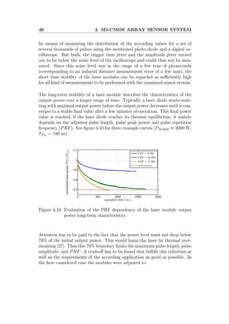
46 4. 3D-CMOS ARRAY SENSOR SYSTEM
by means of measuring the distribution of the according values for a set ofseveral thousands of pulses using the mentioned photo diode and a digital os-cilloscope. But both, the trigger time jitter and the amplitude jitter turnedout to be below the noise level of the oscilloscope and could thus not be mea-sured. Since this noise level was in the range of a few tens of picoseconds(corresponding to an induced distance measurement error of a few mm), theshort time stability of the laser modules can be regarded as sufficiently highfor all kind of measurements to be performed with the examined sensor system.
The long-term stability of a laser module describes the characteristics of theoutput power over a longer range of time. Typically a laser diode starts emit-ting with maximal output power before the output power decreases until it con-verges to a stable final value after a few minutes of operation. This final powervalue is reached, if the laser diode reaches its thermal equilibrium; it mainlydepends on the adjusted pulse length, pulse peak power and pulse repetitionfrequency (PRF ). See figure 4.10 for three example curves (PModule ≈ 2000 W,TPw = 180 ns).
0 500 1000 1500 2000
0.7
0.8
0.9
1
1.1
operation time t in s
norm
alized
lase
rpow
er
P(t
)/P
max
PRF = 5 kHz
PRF = 10 kHz
PRF = 11 kHz
critical level
Figure 4.10: Evaluation of the PRF dependency of the laser module outputpower long-term characteristics
Attention has to be paid to the fact that the power level must not drop below70% of the initial output power. This would harm the laser by thermal over-straining [27]. Thus this 70% boundary limits the maximum pulse length, pulseamplitude, and PRF . A tradeoff has to be found that fulfills this criterium aswell as the requirements of the according application as good as possible. Inthe here considered case the modules were adjusted to

4.2 System Characterization 47
Pulse amplitude: PModule ≈ 2000 W
Pulse length: TPw = 180 ns (⇔ 27 m theoreticalmeasurement range)
Pulse repetition frequency: PRF = 10 kHz
For these settings the equilibrium laser output power levels off at a value shortabove the 70% threshold. Further increase of the PRF causes the laser outputpower to drop below the 70% threshold and thus leads to thermal damageduring longer operation (see output power curve for PRF = 11 kHz ).
4.2.2.4 Eye Safety
The laser produces an intense, high directional beam of light, which can espe-cially harm the eyes of human beings. Therefore, laser sources are classifiedinto laser safety classes from 1 to 4 [28]. Only class 1 guarantees the operationof a laser source without any danger for people (especially their eyes) in thesurrounding. Thus one major goal of the laser module development was theobservance of the regulations for laser class 1. The theoretical limit betweensafe and potentially harmful is called maximum permissible exposure (MPE1)for laser safety class 1. The MPEi – the maximum permissible exposure forlaser safety class i – levels are set by the ’International Commission on Non-Ionizing Radiation Protection’ and are internationally accepted and adoptedby the standardization committees such as IEC TC 76 and ANSI for the re-spective laser safety standards IEC 60825-1 and ANSI Z136.1. MPEi levelsare determined as a function of
• pulse duration,
• pulse repetition frequency (PRF ),
• light emitting area, and
• laser wavelength.
To derive the laser safety class of a laser light source, a measured exposurevalue at a distance of 0.1 m from the light emitter has to be compared to theaccording calculated MPEi value; in the here considered case MPE1.Figure 4.11 shows the measurement result for the UseRCams laser illuminationmodule. Basis for the calculation of the MPE1 are a pulse duration of 180 nsat a PRF of 20 kHz; for the measurement of the radiant exposure coming fromthe laser module, the output power was set to maximum. It homogeneouslydistributes on an illumination field of 30◦x9◦. All values are normalized to the

48 4. 3D-CMOS ARRAY SENSOR SYSTEM
MPE1 (e.g. MPE1(0.1m) =0.00205J/m2), i.e. a normalized exposure valueof 1 or below fulfills the safety class 1 requirements. This condition is notfulfilled for the specified measuring distance of 0.1 m. For measuring distancesof 0.3 m and above it is. To classify the device as class 1 device, it has to beassured, that no human can get nearer to the laser source than 0.3 m, whatis guaranteed under normal operation conditions when the camera is mountedbehind a vehicles windshield. For additionally safety an electronic guard couldbe developed that switches off the laser modules if the vehicle is not moving.
0 0.2 0.4 0.6 0.8 10
1
2
3
4
5
observation distance in m
ener
gy
den
sity
norm
alize
dto
the
MP
E1
MPE
normalized energy density
Figure 4.11: Fulfillment of laser class 1 regulations for different observationdistances
4.2.3 Over-all System Characterization
This chapter characterizes the camera system as a whole after integration of allcomponents. Goal is an overall analysis of the distance measuring capabilitiesof the camera by means of evaluation of different characterizing measurements,which are closely described in the following sections.
4.2.3.1 System Noise / System NEE
Noise investigation
The system noise σU stands for the noise which is inherent to the systemoutput voltage USensor (cf. section 4.1.1.1). As USensor is the measure accessiblefor further processing like distance calculation, this noise value significantlyinfluences the global system performance.Figure 4.12 shows a model for the composition of the noise. Basic components

4.2 System Characterization 49
are the so-called sensor noise σS and the readout noise σR. The sensor noisevoltage is here the standard deviation of the output voltage of the sensor(i.e. sensor noise power is the variance of the sensor output voltage) for asingle accumulation. This noise contains the photodiode noise (σPD−noise),reset switch noise (σRS−noise), shutter switch noise (σSh−noise), source followernoise (σSF−noise), noise of the operational transconductance amplifier (OTA)(σOP−noise), select switch noise (σSl−noise), discharge switch noise (σDS−noise),and accumulate switch noise (σAS−noise). Reference voltages (Uddpix, Uref3, andUref4) also add some noise (σUddpix
, σUref3, and σUref4
). The photodiode noiseconsists of dark photodiode noise and photon shot noise. It must be notedthat all the noise generated in front of the OTA is amplified by the capacitor
ratio CCl
CF, while the OTA noise is amplified by
(1 + CCl
CF
).
The readout noise describes the noise which is added to the sensor signal duringthe readout process. It includes noise contributions from the sensor readoutbuffer (σReadoutBuffer), noise injected due to perturbations on the circuit board(σBoard) and quantization noise (σQuantization) due to signal digitization by theADC.
σUref4
-...
σS
-σPD−noise
-σRS−noise
-σSh−noise
-σSF−noise
-σOP−noise
-σSl−noise
-σDS−noise
-σAS−noise
Sensor (nacc accumulations)
Readout
-σBoard
-σQuantization
-...
σ =√nacc · σ2
SσR σU =
√nacc · σ2
S + σ2R
-σReadoutBufferσUddpix
σUref3
Figure 4.12: Sources of the system noise
Assuming Gaussian distribution (cf. appendix B.2) of the single noise compo-nents, the resulting over-all noise σU is calculated as the square root of thesum of the accumulated sensor noise and the readout noise [29]:
σU =√nacc · σ2
S + σ2R (4.21)

50 4. 3D-CMOS ARRAY SENSOR SYSTEM
with
σS = f(σUddpix, σUref3
, σUref4, σPD−noise, σRS−noise, σSh−noise, σSF−noise,
σOP−noise, σSl−noise, σDS−noise, σAS−noise, ...)
σR = f(σReadoutBuffer, σBoard, σQuantization, ...)
A more thorough noise analysis is a quite complex task. Thus a further re-finement of the noise analysis is not performed here. [30] gives insight into theimage sensors noise behavior.
Noise measurements
Noise measurements were conducted in order to derive the noise characteris-tics of the system. Figure 4.13(a) shows a measurement of σU without laserillumination for different numbers of analog accumulations and shutter length.While the shutter length has no influence on the amplitude of the noise level,the noise increases as expected with increasing numbers of analog accumula-tions. The attempt to fit the function given by equation 4.21 through themeasured curves to derive σS and σR yielded no good results. The reason isthat the noise curves are subject of the same damping as it happens to theprocessed photocharges (cf. chapter 4.2.1.3). Thus in advance of the curvefitting the noise curves have to be weighted with the inverse damping func-tion d(nacc)
−1 of chapter 4.2.1.3. Figure 4.13(b) shows the resulting inverselydamped noise curve for a shutter length of 240 ns and the fitted curve accord-ing to equation 4.21. The parameters of the function that describe σS and σR
are:
σS = 0.379 mV (4.22)
σR = 0.442 mV (4.23)
Figure 4.14 shows the probability density function (PDF, see annex B.1) ofmeasured sensor signal noise values. The histogram is generated from 16000single shutter values at 100 analog accumulations. Result is a Gaussian dis-tribution (compare the histogram to the fitted Gaussian), what justifies the

4.2 System Characterization 51
0 20 40 60 80 100 120 140
0.5
1
1.5
2
x 10−3
nacc
σU
inV
shutter = 30 ns
shutter = 60 ns
shutter = 120 ns
shutter = 240 ns
(a) Dark noise of the system
0 20 40 60 80 100 120 140
1
2
3
4
5x 10
−3
nacc
σU
inve
rsel
ydam
ped
inV
measured
fitted
(b) Dark noise weighted with inverse damping function d(nacc)−1
Figure 4.13: System dark noise mean values original and inversely damped
−0.01 −0.005 0 0.005 0.01 0
0.02
0.04
0.06
0.08
0.1
0.12
U in V
pU
Se
ns
or(U
)
histogram
fitted Gaussian
Figure 4.14: PDF of the dark noise values

52 4. 3D-CMOS ARRAY SENSOR SYSTEM
assumptions given above. The Gaussian property of the signal error distribu-tion will also be of importance for the image processing approach in chapter 6.
Another important measurement is the noise measurement in the presence oflaser illumination. Figure 4.15 shows the result of noise measurements of thesensor output for different illumination values resp. sensor output signals for16 analog accumulations; the illumination strength was thereby changed bytuning the input voltage of the laser illumination module what directly tunesthe module output power.
The additional photon shot noise σPS is derived as follows:
σPS(USensor) =
rQphoto(USensor)·6.242·1018 1
C6.242·1018 1
C·(CD+Csense)
· gSF · CCl
CF(4.24)
Eq. 4.3=
rUSensor·(CD+Csense)· 1
gSF· CFCCl
·6.242·1018 1
C6.242·1018 1
C·(CD+Csense)
· gSF · CCl
CF(4.25)
=
√USensor
6.242·1018 1
C·(CD+Csense)
·√gSF · CCl
CF(4.26)
The resulting overall bright noise σ∗U(USensor, nacc) can then be computed asequation 4.28 shows:
σ∗U(USensor, nacc) =
√√√√nacc ·
(σ2
S +
(σPS(USensor)√
nacc
)2)
+ σ2R (4.27)
=√nacc · σ2
S + σ2R + σPS(USensor)2 (4.28)
Comparing this with the noise as defined in equation 4.21 gives the error inthe computation of σU(nacc) without considering the photon shot noise σPS:
σ∗U(USensor, nacc)
σUD(nacc)
=
√nacc · σ2
S + σ2R + σPS(USensor)2
nacc · σ2S + σ2
R
(4.29)
=
√1 +
σPS(USensor)2
nacc · σ2S + σ2
R
(4.30)

4.2 System Characterization 53
But inserting the values of the capacitors and of the noise contributions σS
and σR known from sections 4.1.1.1 and 4.2.3.1 respectively, results in com-paratively small errors when omitting the photon shot noise. Considering amaximum sensor output voltage of 1.5 V results in a error of 18% for nacc = 1,which is the maximum error value. For increasing values of nacc the errorshrinks rapidely to e.g. 2.7% at nacc = 16 and 0.46% at nacc = 100. Thisshows that especially for high numbers of analog accumulations (i.e. measure-ments where the measurement signals and thus the SNR is low) the photonshot noise can be disregarded compared to the other noise components. Forsimplicity reasons the photon shot noise is not regarded at all in the furtherconsiderations of this thesis; the dark noise value is taken for all computationswithout making much error. Basic equation for noise calculations is thus equa-tion 4.21. This result is important in view of the later image processing, as onecan always suppose the same noise level independently from any illuminationcharacteristics.
−0.2 0 0.2 0.4 0.6 0.8 1 1.2 1.40
0.5
1
1.5
2
2.5
3x 10
−3
µUSensor
in V
σU
inV
Figure 4.15: σU value of the sensor outputs for different sensor signal ampli-tudes
NEE derivation
The sensor noise equivalent exposure NEESensor is defined as the x-coordinatevalue of the intersection point between the interpolated responsivity charac-teristics Rλ and the dark noise of the sensor, i.e. the value of radiant exposurethat generates a sensor output signal which is equal to the sensor noise σS .Analogously a system NEESystem defines the necessary radiant exposure toobtain a sensor output similar to the system noise level σU . As stated earlier

54 4. 3D-CMOS ARRAY SENSOR SYSTEM
in this chapter, the system noise depends on the fixed readout noise and thenacc-dependent sensor noise; the system noise level is defined as the noise atone analog accumulation as this case is the worst case in view of the SNR, ashere the readout noise has the largest influence.
NEESystem|nacc=1 = 225 nJ/m2 (4.31)
NEESensor = 145 nJ/m2 (4.32)
0 1 2 3 4 5 6
x 10−7
0
0.5
1
1.5x 10
−3
radiant exposure in J/m2
US
en
sor,
σU
and
σS
inV
NEESystem = 225 nJ/m2
NEESensor = 145 nJ/m2
extrapolated curve
system dark noise level
sensor dark noise level
Figure 4.16: Determination of the NEE by extrapolating the fitted sensor re-sponsivity curve of figure 4.6
Note that these values are valid for the typical laser light wavelength of λ= 905 nm.For other wavelengths the NEE-values can change due to the λ-dependencyof Rλ.
4.2.3.2 Shutter-Window-Pulse Correlation
The shutter-window-pulse correlation of the 3D-CMOS system was gained bymeasurement and by calculation. For the measurement, the laser pulses triggerwas shifted in time by using a delay element located on the circuit board. Theresulting sensor signal plotted against the laser delay forms the measured corre-lation curve. Additionally, the shutter-window-pulse correlation functions werecalculated as correlation integral of the measured shutter window functions (cf.section 4.2.1.2) and the measured laser pulse shapes (cf. section 4.2.2.1). Theresult of both procedures for a shutter length of 390 ns and a laser pulse lengthof 180 ns is depicted in figure 4.17(a). Only the trailing edge of the function

4.2 System Characterization 55
is shown for reasons of the recognizability of details; the results are the samefor the rest of the curve. In addition to the two curves a straight line is fittedthrough the middle range of the measured curve for linearity investigation,which is shown in figures 4.17(b).
550 600 650 700 750 800 850−0.5
0
0.5
1
1.5
2
Data for fit
laser pulse delay in ns
US
en
sorin
V
measured curve
simulated curve
fitted curve
(a) Trailing edge of the measured and the calculated correlationcurve with linear fit
550 600 650 700 750 800 850−0.1
−0.05
−0.0050.005
0.05
0.1
Linear range
laser pulse delay in ns
dev
iation
from
linea
rity
inV
(b) Deviation of the measured values from the linear fit
Figure 4.17: Shutter-window-pulse correlation investigations
Following results can be gained from the figures:
• The measured correlation curve and the calculated correlation curveagree very well indeed. This means that the sensor model of equation3.16 fits the real behavior of the sensor chip quite well. Thus the calcu-lated sensor output signal can be taken for simulations or the like withoutthe risk of getting large deviations from real sensor signals.

56 4. 3D-CMOS ARRAY SENSOR SYSTEM
• For laser delays between 625 ns and 770 ns the correlation curve exhibitsa range of 145 ns – corresponding to a measurement range of 21.75 m, i.e.for example 2 m - 23.75 m – in which the curve coincides with the fittedstraight line quite good; in this range distance measurement is applicablewithout any further adaption.
• Figure 4.17(b) shows that within the measurement range the deviationof the measured signal from linearity is always below 0.005 V.
• The discrepancies of the shutter functions and the laser pulse shapes fromthe ideal rectangular shape, noted in chapters 4.2.1.2 and 4.2.2.1, do onlyaffect the begin and the end of the edges of the correlation function. Inbetween these corrupted regions good distance measurement is possible.
4.2.3.3 Dynamic Range
Dynamic range is defined as the ratio of the maximum level of a parameter toa minimum detectable value of that parameter.Thus the dynamic range of the photodiode in terms of radiant exposure istheoretically defined as
DRPD,theor = 20 · log
(ESensor,max · TInt,max
NEESensor
)dB (4.33)
for a single accumulation (nacc =1).
Note that this yields (using equation 4.13)
DRPD,theor = 20 · log
(USensor,max
Rλ ·NEESensor
)dB (4.34)
= 20 · log
(USensor,max
σS
)dB . (4.35)
Taking the analog accumulation and digital averaging capabilities of the cam-era system into account the system dynamic range in terms of radiant exposurecan be derived from this as follows:
DRSystem,theor = 20 · log
ESensor,max · TInt,max
NEESystem
nacc,max· 1√
nav,max
dB (4.36)
= 20 · log
USensor,max√nacc,max·σ2
S+σ2R
nacc,max· 1√
nav,max
dB (4.37)

4.2 System Characterization 57
Estimating ESensor,max = 1.5 V (the power supply voltage is only 3.3 V)and taking into account the measured sensor and system noise values σS =0.379 mV and σR = 0.442 mV and the maximum applied number of analogaccumulations nacc = 100 we obtain a dynamic range of the sensor system of
DRSystem,theor = 91.9 dB + 20 · log(√
nav,max
)dB . (4.38)
Now consider the required input range of the camera from the point of view ofthe application specific requirements. In the UseRCams front view applicationthe specified target values are a range of the distance d to be measured from2 m - 20 m and a reflectivity range from 5% - 100% (Lambertian reflectance)at a distance accuracy σd/d of 3%.This leads to following required input range of the camera (see equation 3.11):
20·log
(ESensor,max · TInt,max
NEESystem,min
)= 20·log
(dmax
dmin
)2
︸ ︷︷ ︸distancedynamics
· ρmax
ρmin︸ ︷︷ ︸reflectivitydynamics
· USensor
σU︸ ︷︷ ︸SNRmin
dB
(4.39)
where USensor
σUdefines the signal-to-noise ratio (SNRmin) which even the mini-
mum measured signal has to satisfy to fulfill the 3% distance accuracy require-ment. This SNRmin is derived in the following:
With equations 3.20 and 5.6 one can express the normalized distance accuracyσd/d (use of MDSI3 algorithm assumed, TDL = TDS = 0) as
σd
d=
c2· TPw · 1
(Ua+Ub)2·√U2
a + U2b · σU
c2·(TPw − TPw · Ua
Ua+Ub
) (4.40)
=
1(Ua+Ub)2
·√U2
a + U2b · σU
Ub
Ua+Ub
(4.41)
=1
(Ua + Ub) · Ub
·√U2
a + U2b · σU . (4.42)
As the most critical measurements regarding the signal-to-noise ratio are mea-surements of object which are far away of the camera, equation 4.42 is evalu-ated for high target distances, i.e. Ub → Uc (see figure 3.6) and Ua → U0. Thisyields

58 4. 3D-CMOS ARRAY SENSOR SYSTEM
σd
d|Ub→Uc
Ua→U0
=σU
Ub/c
, (4.43)
and thus
SNRmin =USensor
σU
=d
σd
=1
3%= 33.3 . (4.44)
Hence the required input range of the camera results as
20 · log
(ESensor,max · TInt,max
NEESystem,min
)= 20 · log
((20 m2 m
)2
· 100 %5 %
· 33.3
)dB(4.45)
= 20 · log(66.6 · 103) dB (4.46)
= 96.5 dB (4.47)
Comparison with the theoretical value shows that the system dynamic rangewithout digital averaging (DRSystem,theor = 91.9 dB + 0 dB = 91.9 dB) is notsufficient to cope with the specified input range of the planned applications.Introducing averaging over 3 camera frames (nav = 3) increases the theoreticaldynamic range to 96.7 dB. Hence the camera system fulfills the above men-tioned application requirements if digital averaging over 3 frames or more isapplied. As the DRSystem,theor-value of 96.7 dB exceed the required 96.5 dB(see eq. 4.47) only marginal, the better choice is an averaging value of nav = 4– leading to DRSystem,theor = 97.9 dB – to keep some reserve. This on the otherhand lowers the camera frame rate (cf. section 4.2.3.5) by a factor of 4.
For practical examination of the dynamic range of the camera system measure-ments were conducted for different target distances dr and different target re-flectivities ρ with adaptive number of accumulations nacc (see section 4.1.1.3);from these the standard deviations σdm of the measured distance values dm
were calculated. Figure 4.18 shows the measurement errors normalized to theappropriate target distances dr, i.e. the normalized distance accuracy σdm/dr.Distance derivation algorithm MDSI3 is used.
The curves can now be evaluated according to the above mentioned UseRCamsspecifications. As no target with 100% Lambertian reflectivity could be found(this value is only theoretical; a small fraction of the incident light is alwaysabsorbed by the target), a white paper target with 80% reflectivity was choseninstead. Although for calculation of the dynamic range 100% is set as ρmax,as experiments showed that also for a reflectivity of 100% distance measure-ment over the whole specified measurement range is possible. From figure 4.18

4.2 System Characterization 59
2 4 6 8 10 12 14 16 18 200
1
2
3
4
5
6
7
real target distance dr in m
σd
min
%ofd
r
16100
100
100100 100
100
100
100
100
16 100100
100100 100 100
100100
100
1
44 4
16 16100 100 100
specified error value
5%-target
5%-target; averaged over 4 frames
80%-target
Figure 4.18: Accuracy of the measured distance dm for different targets andcamera parametrizations over a measurement range from 2 m to20 m; the according nacc is added to each data point
one can see, that the 5%-target exceeds the specified error of 3% already fordistances larger then 8 m. Thus the dynamic range is not sufficient to fulfillthe specified requirements without digital averaging, as stated already abovein the theoretical derivation of the dynamic range. But by applying averagingover 4 subsequent frames, the accuracy can be increased what leads to a ful-fillment of the requested values (see figure 4.18). This is a good match withthe theoretical computations.
4.2.3.4 Distance Measurement Performance
Figure 4.19 shows the distance measuring performance of the camera system.Basis is a distance measurement of a plywood target with a reflectivity of∼50%for distances between 3 m and 21 m; pixel 32 of sensor line 6 is examined, sincethis pixel coincides with the center of the target here. Adaptive accumulationis applied with nacc ∈ {1, 4, 16, 64}. This means that at each distance step nacc
is chosen in such way as to get the maximum non-saturated signal.
The blue curve shows the mean values of the measured distances for the dif-ferent distance steps. Good agreement of real with measured distance values(compare measured curve to dashed bisecting line) and good linearity of thedistance measuring characteristics (deviation from the bisecting line, see alsosection 4.2.3.2) can be observed. The green line indicates the standard devia-tion σd of the measured distance values at each distance step. The sawtooth-shaped curve is characteristic for the adaptive accumulation. Each time nacc isincreased to the next level, the distance error drops due to the increased SNR(cf. section 4.1.1.3). The distance error is directly proportional to the target

60 4. 3D-CMOS ARRAY SENSOR SYSTEM
0 5 10 15 20 250
5
10
15
20
25
dr in m
dm
inm
mean measured distance
bisecting line
standard deviation
0 5 10 15 20 250
0.05
0.1
0.15
0.2
0.25
σd
min
m
Figure 4.19: Distance measurement performance using MDSI3 algorithm andadaptive accumulation
reflectivity. Hence to derive the expected distance error for targets with otherreflectivity, the error has to be weighted accordingly.
Besides the good measurement performance described in the previous sectionsalso some shortcomings of the 3D-CMOS sensor system have to be mentionedhere:
• Due to the large pixel dimensions of 130 µm times 300 µm, which arenecessary to collect enough reflected photons in the extremely short in-tegration windows, the resolution of the camera system is comparativelylow. This can cause blurred distance measurement values when one pixel’sees’ two or more different objects. Especially on the edges of objectsthese blurring effects occur.
• The sequential acquisition of the shutters is a drawback when having fastmoving objects in the observed scene, as the two shutters ’see’ actuallydifferent images, as the objects are moving on during the acquisitiontimes of the shutters. Especially on object edges this leads to corrupteddistance measurement results. An improved sensor design implementingalternating acquisition of the single accumulations of the two shutters(what would require additional storage capacitors in the pixel readoutstage) could reduce this effect significantly.
• Scenes with large irradiance gradients on the sensor surface reveal crosstalkbetween the sensor pixels. See chapter 4.2.1.4 for a deeper examinationof this topic.
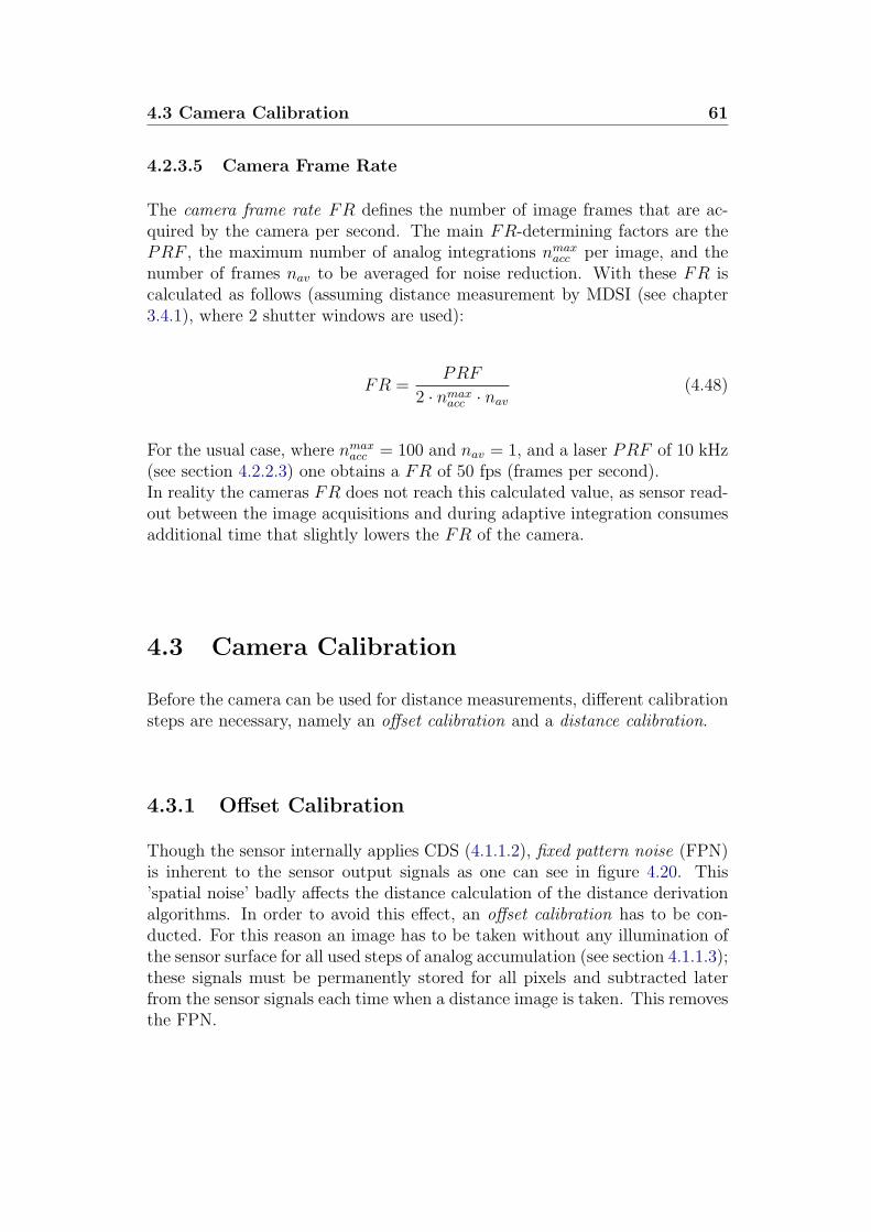
4.3 Camera Calibration 61
4.2.3.5 Camera Frame Rate
The camera frame rate FR defines the number of image frames that are ac-quired by the camera per second. The main FR-determining factors are thePRF , the maximum number of analog integrations nmax
acc per image, and thenumber of frames nav to be averaged for noise reduction. With these FR iscalculated as follows (assuming distance measurement by MDSI (see chapter3.4.1), where 2 shutter windows are used):
FR =PRF
2 · nmaxacc · nav
(4.48)
For the usual case, where nmaxacc = 100 and nav = 1, and a laser PRF of 10 kHz
(see section 4.2.2.3) one obtains a FR of 50 fps (frames per second).In reality the cameras FR does not reach this calculated value, as sensor read-out between the image acquisitions and during adaptive integration consumesadditional time that slightly lowers the FR of the camera.
4.3 Camera Calibration
Before the camera can be used for distance measurements, different calibrationsteps are necessary, namely an offset calibration and a distance calibration.
4.3.1 Offset Calibration
Though the sensor internally applies CDS (4.1.1.2), fixed pattern noise (FPN)is inherent to the sensor output signals as one can see in figure 4.20. This’spatial noise’ badly affects the distance calculation of the distance derivationalgorithms. In order to avoid this effect, an offset calibration has to be con-ducted. For this reason an image has to be taken without any illumination ofthe sensor surface for all used steps of analog accumulation (see section 4.1.1.3);these signals must be permanently stored for all pixels and subtracted laterfrom the sensor signals each time when a distance image is taken. This removesthe FPN.

62 4. 3D-CMOS ARRAY SENSOR SYSTEM
0 10 20 30 40 50 600
0.05
0.1
0.15
0.2
0.25
0.3
pixel-number
Uoffset
inV
line 1
line 2
line 3
line 4
line 5
line 6
line 7
line 8
Figure 4.20: Fixed pattern noise of the sensor chip for 16 analog accumulationsand a shutter length of 240 ns
4.3.2 Distance Calibration
In order to obtain accurate distance values from the raw data of the 3D-CMOScamera, also a distance calibration procedure has to be performed before start-ing measurements. According to the functional principle of the 3D-CMOScamera and the used distance derivation algorithm (cf. chapter 3.4), in the pro-cess of distance calculation an algorithm specific function f(Ui), i ∈ {a, b, c},of shutter signals (MDSI 1: f(Ui) = Ua
Uc, MDSI 3: f(Ui) = Ua
Ua+Ub, etc.) of
each pixel is interpreted as a certain distance value. The right assignmentof quotient to distance value is thereby managed by two so-called calibrationparameters per pixel, which have to be derived using the camera calibrationprocedure.
In a first step images of a plain target at several known distances dr arerecorded, and the appropriate sensor signal function f(Ui) is calculated. Thesecond step is the fitting of a straight line through the measured quotientvalues, which are plotted over the known distances. Thirdly, the slope and in-tercept values (calibration parameters) of the fitted curve are extracted, whatallows an one-to-one mapping of each possible quotient value to a distancevalue. See figure 4.21 to get an example of the above described procedure.
As the calibration parameters slightly differ for different pixels this procedure isconducted for all 64x8 pixels of the imaging sensor at the moment. This and thefact that the camera (or the target) has to be moved during calibration makesthis procedure fairly complex. Further investigations will show, if a simplifiedcalibration procedure, which simulates the different target distances by defined

4.3 Camera Calibration 63
6 7 8 9 10 11 12 130.2
0.25
0.3
0.35
0.4
0.45
0.5
dr in m
quotien
tU
a
Ua+
Ub
measured data
linear fitting
Figure 4.21: Example of a distance calibration measurement curve for 16 ana-log accumulations
delays of the laser pulse, is also feasible with respect to the measurementaccuracy of the camera system.

64 4. 3D-CMOS ARRAY SENSOR SYSTEM

Chapter 5
Optimization of the DistanceMeasurement
5.1 Comparison of the Distance Measurement
Algorithms
In order achieve the best possible measurement results with respect to absoluteand relative measurement accuracy and measuring time, an intensive compari-son of the different distance measurement algorithms (cf. section 3.4) has beenconducted and will be described in this chapter. It includes mathematical in-vestigations, computer simulations, as well as laboratory experiments with the3D-CMOS camera introduced in chapter 4.
5.1.1 Mathematical Investigation
As first investigation method a mathematical derivation of the expected dis-tance measurement error σd is carried out. It enables a fast estimation ofperformance of the employed algorithms, but does not consider some effectsthat occur during the measurement in reality, like non-ideal shutter windowfunctions and laser pulse shapes, signal quantization noise, and the use ofvalue-discrete sensor values for distance calculation. In the following – basedon the well-known law of propagation of uncertainties – the expected distancemeasurement error using the different algorithms is derived; additionally anevaluation example is shown in figure 5.1.

66 5. OPTIMIZATION OF THE DISTANCE MEASUREMENT
5.1.1.1 Propagation of Uncertainties
Let f = f(x1, x2, ..., xn) be a function depending on n variables x1, x2, ..., xn.The uncertainty of each variable is given by ∆xi. Assuming uncorrelatedvariables, the random uncertainty ∆f of f that results from the random un-certainties of the variables can be calculated as:
∆f = ∆f(x1, x2, ..., xn,∆x1,∆x2, ...,∆xn) =
√√√√( n∑1
(∂f
∂xi
·∆xi
)2)
(5.1)
where ∂f∂xi
designates the partial derivative of f for the i-th variable.
This equation is the basis for the mathematical investigation and comparisonof the distance derivation algorithms. Inputs are the sensor output valuesU1, U2, ..., Un, n depending on the algorithm and the according Gaussian dis-tributed signal uncertainties. As the value of ∆Ui is not known in advance, σUi
is used as measure of the signal uncertainty, which is known from the systemnoise measurements in chapter 4.2.3.1. Subsequently one obtains the expectedstandard deviation of the measured distances σd as result. Thus equation 5.1changes to
σd = σd(U1, U2, ..., Un, σU1 , σU2 , ..., σUn) =
√√√√( n∑1
(∂f
∂Ui
· σUi
)2)
. (5.2)
Due to the fact that the signal amplitude Ui has no influence on the signalnoise level σUi
(cf. chapter 4.2.3.1), the noise level for a certain camera setupis measured once and is then valid for any measurement with the accordingcamera settings, yielding
σU1 ≈ σU2 ≈ ... ≈ σUn ≈ σU . (5.3)
In the following, formula 5.2 is evaluated for the different distance calculationmethods described in chapter 3.4:
MDSI1
σd =
√(c
2· TPw ·
1
Uc
· σUa
)2
+
(c
2· TPw ·
−Ua
U2c
· σUc
)2
≈ c
2· TPw ·
1
Uc
·
√1 +
U2a
U2c
· σU (5.4)

5.1 Comparison of the Distance Measurement Algorithms 67
MDSI2
σd =
√(c
2· TPw ·
1
Uc
· σUb
)2
+
(c
2· TPw ·
−Ub
U2c
· σUc
)2
≈ c
2· TPw ·
1
Uc
·
√1 +
U2b
U2c
· σU (5.5)
MDSI3
σd =
√(c
2· TPw ·
Ub
(Ua + Ub)2· σUa
)2
+
(c
2· TPw ·
−Ua
(Ua + Ub)2· σUb
)2
≈ c
2· TPw ·
1
(Ua + Ub)2·√U2
a + U2b · σU (5.6)
MDSI4
σd =
√(c
2· TPw ·
−Ub
(Ua + Ub)2· σUa
)2
+
(c
2· TPw ·
Ua
(Ua + Ub)2· σUb
)2
≈ c
2· TPw ·
1
(Ua + Ub)2·√U2
a + U2b · σU (5.7)
Gradient Method 1
σd =
√(c
2· (TInt,a1 − TInt,a2) ·
−Ua1
(Ua1 + Ua2)2· σUa1
)2
+
+
(c
2· (TInt,a1 − TInt,a2) ·
Ua2
(Ua1 + Ua2)2· σUa2
)2
≈ c
2· (TInt,a1 − TInt,a2) ·
1
(Ua1 + Ua2)2·√U2
a1 + U2a2 · σU (5.8)

68 5. OPTIMIZATION OF THE DISTANCE MEASUREMENT
Gradient Method 2
σd =
√(c
2· (TInt,b1 − TInt,b2) ·
−Ub1
(Ub1 + Ub2)2· σUb1
)2
+
+
(c
2· (TInt,b1 − TInt,b2) ·
Ub2
(Ub1 + Ub2)2· σUb2
)2
≈ c
2· (TInt,b1 − TInt,b2) ·
1
(Ub1 + Ub2)2·√U2
b1 + U2b2 · σU (5.9)
DCSI
σd =c
2·
√(∂TDL0
∂U1
· σU1
)2
+
(∂TDL0
∂U2
· σU2
)2
+ · · ·+(∂TDL0
∂Un
· σUn
)2
(5.10)
with∂TDL0
∂Uibeing calculated according to equation C.8 in the annex.
Figure 5.1 shows the result of the evaluation of the above σd-equations for a vir-tual measurement of distances from 5 m to 20 m. The according shutter signalamplitudes are calculated by means of equations 3.11 and 3.16; the noise levelis taken from the system noise measurement in chapter 4.2.3.1. For reasons ofclarity adaptive accumulation is not considered in the calculation. Though thiswould lower σd for large distances for all of the examined algorithms, it wouldnot change the ratios of the σd. Thus the use of adaptive accumulation has noinfluence on the result of the comparison of the distance derivation methodsexamined here.
As a result it can be seen that especially the gradient methods denoted GRAD1and GRAD2 exhibit bad performance in terms of σd compared to the othermethods. Also MDSI2 shows bad measurement noise behavior; the inaccuracyis here more than twice the inaccuracy of MDSI3 and MDSI4 over long regionsof the measurement range. Thus – according to this mathematical investi-gation – only MDSI1, MDSI3, MDSI4 and DCSI seem to be well suited fordistance measurements.

5.1 Comparison of the Distance Measurement Algorithms 69
5 10 15 200
0.05
0.1
0.15
0.2
0.25
0.3
0.35
d in m
σcalc
din
m
MDSI1
MDSI2
MDSI3
MDSI4
GRAD1
GRAD2
DCSI
Figure 5.1: Calculation of the expected distance measurement accuracy ac-cording to equations 5.4-5.10
5.1.2 Investigation using Simulation
The next step of the comparison of the distance derivation algorithms is a com-puter simulation of the distance measuring process of the 3D-CMOS camerasystem. For good comparability to the mathematical investigation the rangeof the simulation is again 5 m - 20 m; adaptive accumulation is not consid-ered for the above mentioned reasons. Basis for the simulation are calculatedsensor output signal amplitudes (equations 3.11 and 3.16), to which Gaussiandistributed random signals having a standard deviation according to chapter4.2.3.1 are added. These synthetic noisy sensor output values are then pro-cessed for distance calculation using MDSI1, MDSI3, and DCSI, the algorithmsthat showed to be suitable in the mathematical investigation above. Iterationof this procedure for a set of 5000 values leads to the standard deviation of thereceived distance values as shown in figure 5.2.
Result is that the simulation leads to the same results as the calculation, though– in contrast to the calculation – quantization and value-discrete character ofthe sensor signals are considered here. However, these factors seem to haveonly marginal influence on the measured distance at the considered systemsetup.
5.1.3 Experimental Results
From the three methods examined by simulation, only the MDSI algorithmsproved to be suitable for the current 3D-CMOS camera. The reasons for therefusal of the DCSI method are the worse accuracy characteristics and partic-ularly the complexity of the algorithm, i.e. the use of a series of laser pulses for

70 5. OPTIMIZATION OF THE DISTANCE MEASUREMENT
5 10 15 200
0.05
0.1
0.15
0.2
d in m
σsim
din
m
MDSI1
MDSI3
DCSI
Figure 5.2: Simulation of the expected distance measurement accuracy forMDSI1, MDSI3 and DCSI
a single measurement that reduces the camera frame rate below a level whichwould be acceptable for the image processing described in chapter 6.Thus the experimental exploration is directed at the comparison between mea-surement procedures MDSI1 or MDSI3.Until the development of the UseRCams camera prototype, MDSI1 was thedeployed distance derivation method, though the better theoretical noise per-formance of MDSI3 was known. But MDSI3 was not applicable with thepredecessors of the UseRCams 3D image sensor due to insufficient steepness ofthe trailing edge of the shutter window; thus all procedures that make use ofa pulse to shutter window alignment of type b) (according to figure 3.6: thepulse is emitted before the shutter window ’opens’, i.e., the pulse ’moves into’the shutter window for increasing distances resp. τTOF ) were not applicablewith this sensor generation. The trailing edge of these sensors showed a start ofincrease up to 300 ns prior to reaching the final value, what made a reasonablemeasurement of distance dependent sensor signals impossible. The decreasedtrailing edge width of the 3D-CMOS array chip used here of about 60 ns (cp.section 4.2.1.2) makes shutter alignment b) and thus MDSI3 applicable.A measurement was conducted, which determined the standard deviation ofthe measured distance for MDSI1 and MDSI3 at target distances between 3.0 mand 21.0 m in steps of 1.0 m and for different numbers of analog accumulations.Using a plywood target with a reflectivity ρ of ∼50% we got the results shownin figures 5.3 and 5.4.It can clearly be seen that the distance noise using MDSI3 is below the distancenoise using MDSI1 at any distance or integration step. This fact confirms theresults of the accuracy calculations and simulations of the algorithms. To whatextent the ratios between the measured distance accuracy of the two methods

5.1 Comparison of the Distance Measurement Algorithms 71
0 5 10 15 20 25 30 350
0.1
0.2
0.3
0.4
0.5
0.6
0.7
d in m
σd
inm
MDSI1, nacc = 1
MDSI1, nacc = 4
MDSI1, nacc = 16
MDSI1, nacc = 64
MDSI3, nacc = 1
MDSI3, nacc = 4
MDSI3, nacc = 16
MDSI3, nacc = 64
Figure 5.3: Experimental comparison of the distance measurements for MDSI1and MDSI3 (ρ ∼50%)
match with the calculated values is closer examined in figure 5.4 for a mea-surement setup with 16 analog accumulations. The values are normalized withrespect to the measurement accuracy using the MDSI3 method, i.e. the dis-tance noise using MDSI3 is 1.0 for any distance step. The dashed line gives thecalculated error values for the MDSI1 method, the crosses forming the blueline the measured distance errors for MDSI1, which even exceeds the valuepredicted by the calculation and the simulation.
5 10 15 20 250
0.5
1
1.5
2
2.5
3
d in m
σd
/σ
dM
DS
I3
MDSI1, nacc = 16
MDSI3, nacc = 16
calculated
Figure 5.4: Comparison of the measurement result and the calculation resultfor the ratio of the errors of MDSI1 and MDSI3
Thus the calculations, simulations, and measurements correspondingly showedthat the use of MDSI3 is superior due to its good distance error performance

72 5. OPTIMIZATION OF THE DISTANCE MEASUREMENT
compared to all other distance derivation procedures. Serious disadvantages ofMDSI3 did not become evident during a considerable number of test measure-ments under various conditions. Thus MDSI3 was chosen as distance derivationmethod for the UseRCams camera system; also the camera performance mea-surements in section 4.2.3 and the considerations in chapter 6 are based ondistance measurements using MDSI3. See also section 4.2.3.4 for evaluation ofthe system distance measurement performance using MDSI3.
5.2 Further Enhancement Approaches
Besides the internal camera noise, there are also effects from outside the 3D-CMOS camera system, that can negatively influence the measurement result.For the road safety applications, as considered in this thesis, these are envi-ronmental influences as well as sensor saturation caused by highly reflectivetargets. In the following the handling of these perturbations is discussed.
5.2.1 Treatment of Environmental Influences
Environmental influences account for the main group of the exterior pertur-bations of the 3D-CMOS distance image acquisition. They include all kind ofprecipitation, temperature fluctuations, and ambient light.
5.2.1.1 Temperature Fluctuations
At the present state of the system development it was operated at temperaturesbetween 0◦C and 50◦C. The fluctuation of the ambient temperature turnedout to influence the offset of the sensor output signals; for this reason offsetcalibration as described in section 4.3.1 has to be executed when large changesof the ambient temperature (10◦C or more) occur. It has also to be consideredthat the heat dissipation of the laser diodes to the surrounding becomes lessefficient for higher ambient temperatures. The diodes heat up and thus loseoutput power and can even suffer damage (cf. section 4.2.2.3).Further temperature effects are not yet known.
5.2.1.2 Ambient Light
Ambient light, i.e. light from sources different from the laser modules, con-tributes to the photo current of the sensor pixels, and affects the measurementsignal. For this reason correlated double sampling (described in chapter 4.1.1.2)has been introduced into the image acquisition procedure. This means that inaddition to the normal shutter measurement a second measurement with the

5.2 Further Enhancement Approaches 73
same shutter parametrization, but without sending a laser pulse is performed.Subtracting the sensor output signal of this ’dark’ measurement from the sig-nal of the measurement with laser illumination eliminates the influence of anyambient light sources. Prerequisite is that the light emitted by the externalsources is correlated in time over the duration of the two measurements. Asthe measurements are carried out within less than 10 µs, this is obvious forall natural and artificial light sources to be considered here (sunlight, streetlighting, automobile headlights, ...). To make this technique effective, it has tobe ensured that the amount of charges caused by the background light is only asmall fraction of the overall photo charge. Otherwise the sensor dynamic rangecould be seriously reduced. The pulse based measurement technique with in-tegration times in the range of 30 ns to 1 µs and illumination pulses, power ofwhich exceeds the ambient light by a multiple, ensure this at the UseRCamssensor system. Bandpass filters for cutting the laser light wavelength from thelight spectrum – indispensable at the continuous wave approaches [8, 9, 11] –could additionally lower the effect of the ambient light, but they are not reallynecessary.
5.2.1.3 Rain / Snowfall
As it is known, precipitation like rain or snowfall badly influences optical imag-ing systems, especially, if active illumination is used. The reason for this canbe explained by considering the distance ratio of the interfering object (rain-drop or snowflake) and the object to be measured. Thus small objects closeto the camera can reflect more light into the camera objective than a largeobject farther away from the camera (water drop radius typically varies be-tween 102 µm and 104 µm). For clarification figure 5.5 shows the light poweron a single sensor pixel caused by a raindrop with a diameter of 6 mm and byan object with a Lambertian reflectivity of 0.1, which coveres the whole pixel.The raindrop is modeled as a sphere of water, partially reflecting the incidentlight from its surface according to the well-known optical reflection laws. Apart of this reflected light is collected by the camera objective and imaged onthe sensor surface. It can be seen that drops at near distances (0 m - 1 m) caneasily induce higher light power than objects at the usual observation distances(over 2 m).
The effect of such interferences on the distance measurement is shown in figure5.6. Here the measurement result of the distance of an object with a surfacereflectivity of 0.1 at a distance of 8 m is considered under the presence of araindrop. The red curve shows the measured object distance in dependenceof the distance of the raindrop from the camera. The conclusion is that thecorruption of the measured value is very significant up to a distance of 1 m;

74 5. OPTIMIZATION OF THE DISTANCE MEASUREMENT
0 1 2 3 4 5 6 7 810
−12
10−10
10−8
10−6
10−4
10−2
d in m
light
pow
erper
pixe
lin
W
raindrop (diameter 6 mm)
object (whole pixel covered)
Figure 5.5: Radiant power on the sensor surface resulting from a raindrop resp.a Lambertian reflecting object
between 1 m and 2 m a small effect can be observed, for raindrop distancesover 2 m the influence is not significant anymore. Reason for this fast decreaseof the raindrop influence is the constant size of the raindrop in the objectspace for increasing distances. As the raindrop is smaller than a pixel in theobject space, the size of its image on the sensor surface decreases accordingto square law for increasing distances. So does the irradiance induced by theraindrop. The result is a dependence of the light power on the sensor surfacegenerated by the drop, which is proportional to d4. In contrast to the drop theproportionality factor is only d2 for observed objects which totally cover thepixel area in the object space. This is guaranteed for the major part of objectsconsidered in the road safety applications.
0 1 2 3 4 5 6 7 80
1
2
3
4
5
6
7
8
9
dr in m
dista
nce
inm
raindrop-distance
object-distance
measured-distance
Figure 5.6: Measured distance for a object with reflectivity ρ = 0.1 with asingle raindrop in the VOV at different distances

5.2 Further Enhancement Approaches 75
Thus the idea is to suppress the influences by means of shifting the shutterwindow in such a manner that the light reflected from objects in near distancerange does not contribute to the shutter signal. Figure 5.7 illustrates theprocedure. The proposed shutter window shift is only possible for a distancecalculation method using two type b) shutter alignments (cf. figure 3.6). Hencethe gradient method has to be applied. In order to gate a distance range from0 m to dG, the gating time TG has to be adjusted to
TG = 2 · dG
c. (5.11)
Caused by the shutter alignment of the gradient method, a transition regionfollows the gated region, where no measurement is possible, as only one of theshutters gets a signal here. It reaches from dG to dT with
dT =c
2· (TG + ∆TInt) , (5.12)
where ∆TInt, the delay between the two shutter windows, typically lies between5 ns and 50 ns depending on the cameras distance range. After this transitionregion the normal measurement range begins. Measurements are possible upto a distance of
dmax =c
2· (TG + TInt,b1) . (5.13)
Figure 5.8 shows the results of laboratory measurements of a scene consistingof a large target at a distance of 5.0 m and a glass bead in front of the target ata distance of 0.5 m. The 4 mm diameter glass bead acted as rain drop dummyand was hung on a flimsy wire in the VOV of a certain pixel. Several distancemeasurements were conducted for different values of the gating time TG. Ac-cording to the theory (green curve) no influence on the distance measurementshould have been present for gating times above 3.33·10−9 s (correspondingto the bead distance of 0.5 m). But the real measurement yields an influenceup to a TG of 10·10−9 s. This is caused by the non-ideal shape of the shut-ter window function and the laser pulse, introduced in chapters 4.2.1.2 and4.2.2.1. The missing rectangular shape causes blurring of the gating distance.Nevertheless, the measurement error could be lowered by a factor of 10.5 from1.05 m to 0.10 m by introducing a gating time TG of 10·10−9 s.
5.2.2 Saturation Treatment
Independent of the used distance derivation algorithm, sensor saturation canadversely influence distance measurement. This happens if the sense capacitorCsense (see chapter 4.1.1.1) is completely discharged during a single integration

76 5. OPTIMIZATION OF THE DISTANCE MEASUREMENT
t
t
t
EL,ideal(t)
Sensor output signals:
TPw
Shutter alignment b1)
Shutter alignment b2)
TInt,b2
TInt,b1
τTOF,maxτTOF,min
τTOF
TG
TInt,a2
TInt,a1
∆TInt
TG
Ub1(τTOF )
Ub2(τTOF )
with gating of the close-up range:Temporal laser pulse and shutter window alignment for the gradient method
Emitted laser pulse
SλSensor(t)
SλSensor(t)
Figure 5.7: Alignment of a shutter windows relatively to the incident lightpulse at the gradient method with gating of the close-up range
0 2 4 6 8 10
x 10−9
3.8
4
4.2
4.4
4.6
4.8
5
5.2
TG in s
measure
ddista
nce
inm
measured data
ideal measurement curve
Figure 5.8: Distance measurement results for different gating times TG for atarget at 5 m and a glass bead at 0.5 m distance

5.2 Further Enhancement Approaches 77
step, and thus the amount of photo charges generated by the incident light can-not be evaluated. This means that with the actual sensor parametrization adistance measurement is not possible for this pixel. Reason for the saturationis a unusually high irradiance on the sensor surface, which is not covered bythe sensors dynamic range (cf. section 4.2.3.3). It is ether caused by targetsbeing very close to the camera system or by targets with retro-reflective targetsurfaces, because they redirect the incident light to the light source, i.e., thelaser light emitted by the camera is directly reflected to the camera. Comparedto Lambertian reflecting targets, which reflect the incident light into the wholehalf-sphere over the target surface, the resulting irradiance on the sensor chipcan reach values up to a few 100 times higher at equal target distances.A technique was developed in order to manage distance measurement for sat-urated pixels. The approach is similar to the gating approach above; alsohere the gradient method is applied. In order to decrease the generated photocharge, the overlap between laser window and shutter pulse is decreased byshifting the laser pulse by means of a electronic delay component on the sensorboard. This procedure is done according to a certain shift pattern, until unsat-urated sensor signals are received that allow distance calculation. Disadvantageof this algorithm is the increased time consumption; several measurement stepscan be necessary to receive unsaturated sensor signals. Also the measurementaccuracy drops due to the use of the gradient measurement method (cf. section5.1.1)The procedure was successfully tested in the laboratory; yet it was not imple-mented in the standard sensor firmware. The reason is that the above men-tioned time consumption of the saturation mitigation algorithm is not feasiblewith the presently available budget of laser pulses, i.e. the technique lowersthe frame rate of the system too much.

78 5. OPTIMIZATION OF THE DISTANCE MEASUREMENT

Chapter 6
Novel 3D Real-Time ImageProcessing Approach
Classical 3D real-time image processing is usually based on stereo images [5],and thus suffers from the problems mentioned in 2.2.2.1. Very few applicationsin 3D image processing rely on direct distance image acquisition: a rare exam-ple are geometry acquisition systems which employ scanning methods [14], e.g.for machine vision. They, however, are cumbersome and slow. Since the 3Dcamera presented in this work provides 3D real-time images, a new approachto real-time 3D image processing had to be developed in this work [31]. Goalis thereby the extraction of the needed information from the raw data andproviding it in an appropriate data format. These procedures are subject ofthe following chapters. Background is the use of the camera in road safetyapplications as described in chapter 1; though the described procedures couldalso be applied to many other tasks of todays computer vision. The basic flowof the proposed image processing is shown in figure 6.1.
Result
Lists
Distance
Images
processingKalmanFiltering
Pre-processing
Post-
Classification andAction EstimationTrackingSegmentation
Figure 6.1: Image processing chain
The image processing chain is divided into three main tasks, which are repeatedfor each image frame in real time, i.e. parallel to the image acquisition of the

80 6. NOVEL 3D REAL-TIME IMAGE PROCESSING
3D-CMOS camera. First part is the segmentation of the images, that mainlyaims at the isolation and position determination of objects from single 3Dimages. Following the tracking module performs Kalman filtering to derivefurther object properties like velocity or even acceleration extracted from thetemporal movement of an object over a sequence of frames. The last step is theprocessing of the entire information for classification of the detected objectsand action prediction that should give a reliable prediction of the movementsof the object in the next moments.
6.1 Raw Data Properties
Basis for the image processing are the raw data delivered by the 3D-CMOScamera. What differs from conventional 2D image processing, where onlyamplitude values – representing gray scale values or colors of the observedscene – are available for each pixel, is that additional distance information ispresent here and can be utilized in the image processing algorithms. Further,the raw data contain the number of analog accumulations (cf. section 4.1.1.3)that were used for the acquisition of the corresponding pixel signal. Togetherwith the knowledge of the systems noise behavior described in chapter 4.2.3.1,the expected standard deviation of the sensor signals and the resulting distanceuncertainty value can be derived (chapter 5.1.1). This capability will be utilizedin section 6.4.3.3.Thus the pixels raw data contain the following information as input to theimage processing chain:
• Pixel position in pixel coordinates
• Distance value
• Sensor signal amplitudes
• Number of analog accumulations
6.2 Coordinate Systems and Coordinate Trans-
formations
For description of the image acquisition with the 3D-CMOS camera and theimage processing, the introduction of several different coordinate systems isnecessary. Even though each coordinate system (CS) itself enables the de-scription of point coordinates in the 3D-space sufficiently, switching between

6.2 Coordinate Systems and Coordinate Transformations 81
different CSs during the image acquisition and processing processes is unavoid-able for reasons of observational clearness, computational efforts or feasibilityin potential applications. If the relative position between two CSs is known,point coordinates can be transformed arbitrarily between them. In the follow-ing the here used coordinate systems as well as the transformation rules aredescribed.
6.2.1 Pixel and Sensor Coordinate System
The fundamental CS of the 3D-CMOS camera is the pixel coordinate system,since the camera raw data on sensor level are represented in pixel coordinates.A point position PP is here described by three coordinates (see figure 6.2):The first two are the horizontal (defining the sensor pixel column) and the ver-tical (defining the sensor pixel row) pixel index uP and vP respectively, whichdescribe the sensor plane position of the projection of a real-world object point.Third is the distance dPP
measured for the according pixel. Thus no furtherknowledge of sensor or camera geometry is necessary for a unique localizationof a point in the 3D-space. Up to the end of the segmentation, all image pro-cessing is performed on the level of the pixel CS.
Quite similar to the pixel CS is the sensor coordinate system, which is alsodepicted in figure 6.2. A point position in sensor coordinates is described bymeans of two coordinates xSP
and ySP, assigning the position of the points
image on the sensor surface, and the measured distance dSP= dPP
. xSPand
ySPare measured from an arbitrary origin on the sensor plane; normally the
intersection point of the cameras optical axis and the sensor surface is assignedas origin.
ys
u
v
M
+ (dPP= dSP
= dP )
xs
Figure 6.2: Pixel and sensor coordinate systems
In order to convert the representation of a point P from pixel to sensor coor-

82 6. NOVEL 3D REAL-TIME IMAGE PROCESSING
dinates, following transformation has to be conducted:
PS =
xSP
ySP
dP
=
(uP − uM) ·∆x
(vP − vM) ·∆y
dp
(6.1)
where ∆x and ∆y define the horizontal and the vertical pixel pitch of the imagesensor. Thus the knowledge of the sensors geometrical parameters is necessaryfor this transformation.
6.2.2 Camera and Reference / World Coordinate Sys-tems
yW
φM
W
xWzW
zC
yC
xC
P
f
C
Sensor
plane
P’
d = CP
xS
yS
θ
Figure 6.3: Sensor, camera, and world coordinate systems
The camera coordinate system represents points in common Cartesian coor-dinates xC , yC and zC . As figure 6.3 shows, its origin C is located in theoptical center of the camera, i.e. in the center of the imaging lens. The x-axisis oriented along the optical axis of the camera, the y-axis to the left, lookingin positive x-direction, and the z-axis upwards, each forming an angle of 90◦
between each other. This results in a clockwise oriented Cartesian coordinatesystem. Point representation in camera coordinates is used in the trackingmodule of the image processing procedure. The transformation from sensorcoordinates is described below.With f being the focal length of the camera imaging optics one can derive theangles φ and θ describing the angle between the view ray to a point P and thexz-plane resp. xy-plane. Thus one obtains an polar point description PS′ of P

6.2 Coordinate Systems and Coordinate Transformations 83
based on the sensor coordinate description.
φ = arctan
(xSP
f
)(6.2)
θ = arctan
(ySP
f
)(6.3)
PS′ =
φ
θ
dP
(6.4)
Starting with this description, the transformation from sensor to camera coor-dinates of a scene point P is executed by following equation:
PC =
xCP
yCP
zCP
=
d · cos(φ) · cos(θ)
d · sin(φ) · cos(θ)
d · sin(θ)
(6.5)
As in most applications the camera coordinate system is not the reference,which position values are related to, the point coordinates in camera coordinaterepresentation have to be related to a reference coordinate system. This CS –often called world coordinate system – is also clockwise oriented and Cartesianand is defined in the application using the 3D data. In the UseRCams front-view application (see chapter 1) for instance, the reference system is a vehicleinherent coordinate system with its origin being located on floor level on theintersection point of the axes in longitudinal and transverse directions of thevehicle; the x-axis is directed parallel to the longitudinal axis. Its relativeposition to the camera CS is described by a translation vector T and a rotationmatrix R [32].
PC =
xCP
yCP
zCP
= R ·
xWP
yWP
zWP
+ T = R · PW + T (6.6)
with T being the translation vector between the coordinate system origins Wand C represented in world coordinates

84 6. NOVEL 3D REAL-TIME IMAGE PROCESSING
T =
xWC
− xWW
yWC− yWW
zWC− zWW
=
xWC
yWC
zWC
, (6.7)
and R the rotation matrix describing the orientation of the camera and thusalso of the camera image with respect to the world CS. It can be assembledfrom three elementary rotation around the three coordinate system axes [33].
R(ψ, θ, φ) = Rx(φ) ·Ry(θ) ·Rz(ψ) = (6.8)
=
cos(θ) cos(ψ) cos(θ) sin(ψ) − sin(φ)
sin(φ) sin(θ) cos(ψ)− cos(φ) sin(ψ) sin(φ) sin(θ) sin(ψ)− cos(φ) cos(ψ) sin(φ) cos(θ)
cos(φ) sin(θ) cos(ψ)− sin(φ) sin(ψ) cos(φ) sin(θ) sin(ψ)− sin(φ) cos(ψ) cos(φ) cos(θ)
(6.9)
where ψ, θ and φ denote the rotation angles around the coordinate axes. Thecompliance of the order of the three basic rotations is mandatory to obtain theright rotation matrix R.
Analogous to equation 6.6, the transformation from a point in camera coordi-nates to world coordinates is carried out by applying equation 6.10:
PW =
xWP
yWP
zWP
= R−1 ·
xCP
yCP
zCP
− T
= R−1 · (PC − T ) (6.10)
6.3 Object Segmentation
The first stage of the image processing chain is the spatial segmentation ofthe 3D raw images on single frame level. Goal is a reliable partitioning ofthe images into a set of sub-regions, each of them representing a single ob-ject in the VOV of the camera. In contrary to 2D image segmentation [34,35],where segmentation is based on color, signal amplitude or texture, the (x, y, z)-information of each pixel is used here as basic decision criterion for segmenta-tion algorithms. Thus effects of lighting conditions or object surface propertieson the segmentation results are not considered.
The proposed algorithm performs following processing steps:

6.3 Object Segmentation 85
• Data preparation:Here the raw data are preprocessed for the segmentation. First 3x1or 3x3 median filtering [36] is performed, what proved to be useful toreduce noise and outliers that are due to edge effects, adverse objectsurface properties (reflective/retro-reflective), and other effects. For theUseRCams front view application a subtraction of the floor level is alsoaccomplished, where all pixels, that are supposed to image a part of thefloor are removed from the image frame (only objects different from thefloor level are of interest in this application). The decision if a pixel isimaging a part of the floor is done by a comparison of the pixels distancevalue with a stored floor plane, which is either taken from an earlieracquired image of the floor or calculatively derived from the knowledgeof the cameras position and rotation in the reference coordinate system.Compare the two lower pixel lines of figures 6.5(e) and 6.5(f) to see theeffect of the floor level subtraction on example scene in figure 6.5(d).
• Segmentation:The actual segmentation is done by a region growing algorithm [36], asregions exhibiting similar distance values in the raw image must belongto the same object in the cameras VOV with high probability. Startingat an arbitrary image point (in practice one of the image corners), thealgorithm goes through the image pixel by pixel. For each pixel with avalid distance value, the adjacent pixels are checked for region affiliation.The criterion if the pixel belongs to the region or not is the differencebetween the distance value of the pixel and the present mean distanceof the object, which has to be lower than an adjustable threshold. Ifa pixel (exhibiting the measured point coordinates PPi
, i ∈ {u, v, d})is found to be the nth member of the current object, an update of theobject position coordinates POi
is performed:
P ′Oi
=POi
· (n− 1) + PPi
n, i ∈ {u, v, d} (6.11)
Analogously, also other object description parameters (see table 6.1) areupdated.Two segmentation examples for a synthetic model scene and a real sceneare given in figure 6.5. Each starts with a 2D image of the scene (fig.6.12(a) and fig. 6.5(d)), giving the reflectivity and shape properties of thescenes objects. Secondly, the raw 3D images are given for both scenes (fig.6.12(b) and fig. 6.5(e)); the distance value measured by a pixel is codedin the pixel color. The distance measurement noise is clearly visible inthe changing pixel color within the objects. White areas do not contain

86 6. NOVEL 3D REAL-TIME IMAGE PROCESSING
pixels with valid distance values, which means in the most cases thatno signal was received as no object is reflecting the emitted laser light.Last figures 6.5(c) and 6.5(f) show the segmented images. The objectscontained in the above figures are accurately isolated as image regions,the position in pixel coordinates (u, v, d) and the number of pixel (NPix)the object consists of are given by the associated text.
• Output:As information source for the following image processing steps (trackingand classification), the segmentation algorithm outputs a list contain-ing object description records for all objects found in the current frame,called object list (OL) of the k-th frame, OL(k). Additionally someglobal parameters like the acquisition time tacqu of the corresponding im-age frame and the number of objects NO contained in the OL are stored.Figure 6.4 shows the basic structure of an OL and the essential contentsof a object description record; table 6.1 explains these parameters.
OL(k)
NO
tacqu
O1
O2...
...Om
Oi
Oi
PO
US
NPix
hO
wO
NInt
Figure 6.4: Structure of the object list of an image frame

6.3 Object Segmentation 87
Table 6.1: Main parameter of the description format for segmented objects
Parameter Description
PO Position of the object centroid in pixel coordinates
wO Object width in pixels
hO Object height in pixels
NPix Number of pixels the object consists of
NInt Average of the analog integrations used for image acqui-sition over all object pixels
Us Average of the sensor signal amplitude over all objectpixels

88 6. NOVEL 3D REAL-TIME IMAGE PROCESSING
(a) Synthetic scene
(b) Synthetic 3D-CMOS depth image of the sceneabove
(c) Result of the segmentation of the synthetic depthimage
(d) Real scene
(e) 3D-CMOS depth image of the real scene
(f) Result of the segmentation of the real depth im-age
Figure 6.5: Segmentation examples of synthetic and real depth images

6.4 Object Tracking 89
6.4 Object Tracking
Object tracking includes all processing steps that account for the tracing andthe extraction of state parameters of moving objects based on a sequence ofobservations over time. Several techniques – applied on 2D camera data, radardata, or the like – are known in literature [37,38,34].Accordingly the object tracking module developed in this work was designedfor the tracing and the extraction of kinematic parameters – including objectposition, velocity and acceleration – of segmented objects in the image framesequences of the 3D-CMOS camera. The tracking procedure is divided intothree parts, namely preprocessing, Kalman filtering, and postprocessing (cf.figure 6.1), which are addressed in the following sections.
6.4.1 Preprocessing
To provide the information necessary for the Kalman filtering, several prepro-cessing steps have to be carried out. They include:
• Coordinate transformation from pixel to reference coordinates accordingto section 6.2; in the case considered here the reference coordinate systemis a vehicle inherent coordinate system (c.f. section 6.2.2). From here anyposition or distance measures are given in Cartesian coordinates.
• Evaluation of the time T elapsed between the last and the current imageframe:
T = tacqu(k)− tacqu(k − 1) , k ∈ N (6.12)
with tacqu(k) being the point of time of the acquisition of the k-th frame.
• Frame to frame object recovery
While the coordinate transformation and the evaluation of T are trivial math-ematical operations performed on the output data of the segmentation proce-dure, the recovery of the objects of the last frame in the current frame, requireselaborate image processing, which is described below.
6.4.2 Frame to Frame Object Recovery
The frame to frame object recovery procedure (also known as tracing) linksthe single frames of an 3D image sequence to each other. Basis are the objectlists generated during segmentation. Goal of this procedure is the reliableassignment of objects contained in the object list OL(k − 1) of the last frameto the objects contained in the object list OL(k) of the current frame (fig.

90 6. NOVEL 3D REAL-TIME IMAGE PROCESSING
6.6). This tracing of objects over a sequence of 3D image frames is an essentialpart in the proposed image processing approach. Wrong assignments entirelydistort the tracking results and thus influence the scene recognition capabilityof the camera system in a very severe way. Sections 6.4.2.1 and 6.4.2.2 describethe algorithms implemented to solve this task.
OL(k + 1)
99K 99KO1
O2
On
...
O1
O2
Om
...
O1
O2
Ol
...
NO
tacqu
OL(k)
NO
tacqu
NO
tacqu
OL(k − 1)
Figure 6.6: Series of consecutive object lists for the (k − 1)-th, the k-th, andthe (k + 1)-th time step
6.4.2.1 Inter-Object Distance Computation
The object recovery algorithm developed in this work is based on the evaluationof the distance between the centroids of the objects of the (k − 1)-th and thek-th frame. As distance between two centroids P and S at position ~s and ~prespectively one could choose the Euclidean distance
aE =
√√√√ n∑i=1
(pi − si)2, (6.13)
with n being 3 in the here considered case for the three dimensions x, y, andz of the Cartesian space.
But using this distance computation method, it is not possible to weight themeasurements acquired for different spatial directions. This is necessary, how-ever, since the quality of distance measurement for the different spatial dimen-sions x, y, and z varies. A large measurement variance is an indication of noisy,and ,therefore, inaccurate determination of that particular spatial dimension.For this reason it should be handled in a different way than a measurementof another spatial dimension exhibiting small variance, which is obviously lessnoisy and thus more reliable. Using the Mahalanobis distance instead solves

6.4 Object Tracking 91
this problem as weighting of the distance components is performed here. TheMahalanobis distance between P and S is computed by equations 6.14-6.15;thereby the component distances (pi − si) are weighted with the reciprocal ofthe according distance measurement noise σx, σy, or σz. This accounts for thevariations in distance measurement due to the measurement noise.
aM =
√(~p− ~s)T S−1(~p− ~s) (6.14)
with
S−1 =
1σx
0 0
0 1σy
0
0 0 1σz
(6.15)
As shown in figure 6.7, all points with equal Mahalanobis distance aM lie onthe surface of a 3-dimensional ellipsoid with the three radii rx, ry, and rz whichcorrespond to the diagonal elements of matrix S.
x
xS3
rx
xP
rz
ry
xS2
xS1
z
y
Figure 6.7: Example ellipsoid of constant Mahalanobis distance

92 6. NOVEL 3D REAL-TIME IMAGE PROCESSING
6.4.2.2 Object to Object Assignment
For assigning an object i of OL(k−1) to an object j of OL(k) the Mahalanobisdistance (see equation 6.14) between O(i) of OL(k − 1) and O(j) of OL(k) iscomputed for all j. If the lowest of these distances is lower than an adjustabledistance threshold, O(j) of OL(k) is assumed to be the same object as O(i) ofOL(k − 1).Once an object O(j) of OL(k) is assigned, it is not available for further as-signments anymore. As measure for the ’age’ of an object the number ofassignments, i.e. the number since how many frames the object exist is storedin an object associated counter.In order to prevent wrong assignments that ’snatch away’ the potential suc-ceeding objects, prioritization rules for the order of object assignments areimplemented. Basis for the prioritization is a priority value that is computedfrom
• the object age (counted in frames),
• the number of pixels NPix the object consists of, and
• the reliability of the measurement derived from US and NInt (cf. table6.1).
As a result of the object recovery procedure each object contained in OL(k) iseither assigned to an object of OL(k − 1) or identified as a new object, thatappeared the first time in the current frame. This information is then used bythe Kalman filter introduced below.
6.4.3 Kalman Filtering
Kalman filtering [39, 40] basically yields the best possible estimation of thepresent state of a time-varying system. Sources of information are therebyknowledge about the temporal behavior of the system and state measurements,which contain information about the system states plus inherent measurementnoise, which is unavoidable for observations of any physical process. Retrievingthe available information during minimizing the influence of the noise is thusthe goal of the Kalman filtering operation. The Kalman filtering approach ofthis work is closely described below, following [41] and [42].
6.4.3.1 Process Description
The process to be estimated has to be discrete-time controlled and describableby a linear differential equation as shown in equation 6.16. Here the considered

6.4 Object Tracking 93
process is the movement process of objects in the VOV of the camera. Byadequate choice of the equation parameter, the process is being modeled asgood as possible.
x(k) = A(k) · x(k − 1) + B(k) · u(k − 1) + w(k − 1) , (6.16)
with
x(k) : n-dimensional system state vector, x ∈ Rn at the k-th time step
u(k) : l-dimensional control input vector, u ∈ Rl at the k-th time step
w(k) : n-dimensional process noise vector, w ∈ Rn at the k-th time step
A(k) : n× n-dimensional state transition matrix at the k-th time step
B(k) : n× l-dimensional matrix relating u to x at the k-th time step
The state vector x(k) of the system is the smallest dimension vector thatcontains all the parameters of the system which are of interest in the accordingcase of use. In the here considered application, the object position (x, y, z),velocity (x, y, z), and acceleration (x, y, z) in all three space dimensions are thesubjects of interest, i.e. a 3-dimensional accelerated object movement model isused. This leads to the 9-dimensional state vector:
x(k) =
xx(k)
xy(k)
xz(k)
9×1
where xx =
x(k)
x(k)
x(k)
, xy =
y(k)
y(k)
y(k)
and xz =
z(k)
z(k)
z(k)
(6.17)
The state transition matrix A(k) relates the system state at the (k − 1)-thtime step to the system state at the k-th time step according to the physicalbehavior of the system. Thus for the accelerated movement model in the 3-dimensional space one obtains by applying the well-known Newtonian motionequations :
A(k) =
Ax(k) 0 0
0 Ay(k) 0
0 0 Az(k)
9×9
, Ai(k) =
1 T 1
2T 2
0 1 T
0 0 1
(6.18)
Analogously to A, B relates the optional control input u to the system state.In the considerations of this work no control input is present at any time, i.e.

94 6. NOVEL 3D REAL-TIME IMAGE PROCESSING
u(k) = 09×1∀k ∈ N. This means that the expression B(k) · u(k − 1) does notinfluence the equation and is thus omitted in the following.
The noise vector w(k) describes the noise of the process at the k-th timestep. It is a very important part of the process model, as it models the uncer-tainty of the object movements, i.e. the deviation from the course describedby matrix A. For the description of process noise the piecewise constant ac-celeration increment model [42] was chosen. This models the acceleration as aWiener process, i.e. process with independent increments, which are modeledas zero-mean white noise. Thus the single noise contributions are assumed asuncorrelated. The process noise vector is:
w(k) =
wx(k)
wy(k)
wz(k)
9×1
, wi(k) = Γ(k) · wi(k) =
12T 2
T
1
· wi(k) (6.19)
p(w) ∼ N(0,Q) (6.20)
The conducted measurements result in a measurement vector z ∈ Rm, whichis here, like in most systems, different to x, as not all system state variablesare accessible to direct measurement. The matrix H relates the state vectorto the measurement vector as described by equation 6.21.
z(k) = H · x(k) + v(k) (6.21)
with v being additive measurement noise, assumed to be white, uncorrelatedand normally distributed:
p(v) ∼ N(0,R) (6.22)
In the here considered case H is
H =
1 0 0 0 0 0 0 0 0
0 1 0 0 0 0 0 0 0
0 0 1 0 0 0 0 0 0
(6.23)
6.4.3.2 Basics of Kalman Filtering
State estimation based on Kalman filtering is a recursive process according tofigure 6.8, that consists of a prediction and a correction step. Basic principleis the sophisticated combination of the knowledge about the object history

6.4 Object Tracking 95
and its expected behavior (time update) and the new information introducedby the measurement result (measurement update). Each time a new measure-ment result z(k) is available, a prediction/correction-cycle is performed for thederivation of the corresponding estimate x(k).
Measurement Update(Prediction)Time Update
(Correction)
Figure 6.8: Kalman filter principle
Derivation of the Kalman Filter Equations
Let x− be the a priori and x the a posteriori state estimate of a system statevector x, where x− indicates the state determined in the time update and xthe result of the measurement update. The errors of the a priori and the aposteriori state estimates, i.e. their deviations from the state x(k), are definedby
e−(k) = x(k)− x−(k) (6.24)
e(k) = x(k)− x(k) . (6.25)
From this one obtains the a priori respectively a posteriori error covariance ma-trix P−(k) and P (k) as autocovariance matrix of e−(k) and e(k)(E[·]: expectation):
P−(k) = E[e−(k)e−(k)T ] (6.26)
P (k) = E[e(k)e(k)T ] (6.27)
The Kalman filter cycle starts with the time update. It contains two steps, theprediction of the new a priori state estimate x−(k) state by inserting x(k − 1)into equation 6.16 and the update of the of its error covariance matrix P−(k).The according formulas are shown in figure 6.9 in the time update box. Initial-ization of x(k − 1) and P (k − 1) has to be done at the first run of the cycle;different procedures for that are proposed in literature [42,43].

96 6. NOVEL 3D REAL-TIME IMAGE PROCESSING
Following the measurement update is executed. It contains the computation ofthe so-called Kalman gain K, the calculation of the a posteriori state estimatex – the actual Kalman filter output – as a linear combination of the a prioriestimate x−(k) and a weighted difference between an actual measurement zand a measurement prediction (Hx−), as well as the update of the a posteriorierror covariance matrix P (k). The measurement update box in figure 6.9 showsthe three equations, [39,40,43] give a close description of the derivation of them,especially of the weighting factor K (Kalman gain).
x(k) = x−(k) + K(k)(z(k)−Hx−(k))
Measurement Update (Correction)
Time Update (Prediction)(1) Compute the Kalman gain
(2) Project the error covariance ahead
(1) Project the state ahead
P−(k) = A(k)P (k − 1)A(k)T + Q(k)
x−(k) = A(k)x(k − 1) (2) Update estimate with measurement zk
K(k) = P−(k)HT (HP−(k)HT + R(k))−1
(2) Update the error covariance
P (k) = (I −K(k)H)P−(k)
Figure 6.9: Kalman filter formulas
6.4.3.3 Derivation of the Noise Covariance Matrices Q(k) and R(k)
As defined in equations 6.20 and 6.22, in Kalman filtering the uncertaintiesof the observed process and the uncertainty of the Kalman filter inputs, i.e.the measurement results z(k), are described by the noise covariance matricesQ(k) and R(k). While the process description matrix A(k) is governed byphysical laws describing the system (cf. equation 6.18) and H only containsassignment rules between the measurement vector components and the statevector components, Q(k) and R(k) are the two parameters that directly in-fluence the dynamical behavior of the Kalman filter. Thus it is important toreproduce the reality as good as possible when determining these matrices inorder to obtain good filtering results. On the other hand specific changes ofQ(k) and R(k) allow tuning of the estimation behavior of the filter (see filtertuning in chapter 6.4.3.4). The following paragraphs show the derivation of

6.4 Object Tracking 97
Q(k) and R(k) in view of the traffic object tracking task considered in thisthesis.
The Process Noise Covariance Matrix Q(k)
Q(k) describes the random input of an observed process, i.e. the deviationsof the process from the behavior described in the process description matrixA(k), as they are expected in almost every real system. In the here consideredcase of the estimation of position, velocity and acceleration of an object in allthree dimensions of space, Q(k) is a 9× 9 matrix, that consists of three 3× 3sub-matrices, which are located on the matrices diagonal, as shown in equation6.28.
Q(k) =
Qx(k) 0 0
0 Qy(k) 0
0 0 Qz(k)
(6.28)
Using the piecewise constant acceleration increment model as introduced in6.4.3.1, the process noise covariance sub-matrix Qi results as
Qi
[29]= E[(wi(k)− E[wi(k)]︸ ︷︷ ︸
=0
) · (wi(k)− E[wi(k)]︸ ︷︷ ︸=0
)′] (6.29)
= E[wi(k) ·wi(k)′] (6.30)
Eq.6.19= E[(Γ(k) · wi(k)) · (Γ(k) · wi(k))
′] (6.31)
= Γ(k) · σ2wi· Γ(k)′ (6.32)
=
14T 4 1
2T 3 1
2T 2
12T 3 T 2 T
12T 2 T 1
· σ2wi
, (6.33)
with T being the time elapsed between the (k − 1)-th and the k-th time step.The values of the σwi
have to be closely investigated in order to determinethe parameters of the Kalman filter correctly. See chapter 6.4.3.4 for a deeperinvestigation of this of this topic.

98 6. NOVEL 3D REAL-TIME IMAGE PROCESSING
The Measurement Noise Covariance Matrix R
To derive the measurement noise covariance matrix R, we start with a noiseanalysis on sensor level, as is obvious, that the three basic measurement noisecomponents are related to the three dimensions of a point in sensor coordi-nates. Thus the basic noise components are noise of the determination of thecoordinates of a point on the sensor surface (angular noises σφ and σθ accord-ing to figure 6.3) and noise of the distance measurement (distance noise σd).As a good approximation these values are assumed as zero mean and uncor-related between each other. Hence one obtains following covariance matrix ofthe measurement noise in polar sensor coordinates:
RS =
σ2
φ 0 0
0 σ2θ 0
0 0 σ2d
(6.34)
As this representation of the measurement noise is not of use for the consideredKalman filtering approach on the basis of object movements in a Cartesianspace (world coordinates), RS has to be translated to the world coordinatesystem [44]. The result is the measurement covariance matrix R described byequations 6.35-6.37.
R =
σ2
vxCov(vx,vy) Cov(vx,vz)
Cov(vx,vy) σ2vy
Cov(vy,vz)
Cov(vx,vz) Cov(vy,vz) σ2vz
(6.35)
where
σ2vi
= σ2φi
+ σ2θi
+ σ2di
, i ∈ {x, y, z} (6.36)
Cov(vi,vj) = σφi· σφj
+ σθi· σθj
+ σdi· σdj
, i, j ∈ {x, y, z} , i 6= j (6.37)
A noise component σpc in equations 6.36 and 6.37 represents the noise of themeasurement of coordinate p, p ∈ {φ, θ, d} in polar representation that reap-pears in the noise of coordinate c, c ∈ {x, y, z}, in Cartesian representation.The 9 different σpc for all possible combinations of polar and Cartesian coor-dinates are displayed in table 6.2.

6.4 Object Tracking 99
Table 6.2: Component noise contributions σpc for σφ � 1 and σθ � 1
x y z
φ σφx = d · σφ · sin(φ) σφy = d · σφ · cos(φ) σφz = 0
θ σθx = d ·σθ ·cos(φ) ·sin(θ) σθy = d ·σθ ·sin(φ) ·sin(φ) σθz = d · σθ · cos(θ)
d σdx = σd · cos(φ) · cos(θ) σdy = σd · sin(φ) · cos(θ) σdz = σd · sin(θ)
Thus the calculation of the basic noises σφ, σθ, and σd is crucial for a properfunctionality of the Kalman filter. They depend on several system parameters,the segmentation results of the observed object, as well as on the utilizeddistance calculation procedure. 6.38-6.40 show the set of equations; use ofdistance derivation method MDSI3 (cf. chapter 3.4) is assumed. Using otherdistance derivation methods the deviation of the distance measurement σd hasto be adapted according to section 5.1.1.1.
σφ =
∣∣∣∣arctan
(xs
f
)− arctan
(xs + σxs
f
)∣∣∣∣ (6.38)
with σxs
Eq. 6.1= σu ·∆x
σθ =
∣∣∣∣arctan
(ys
f
)− arctan
(ys + σys
f
)∣∣∣∣ (6.39)
with σys
Eq. 6.1= σv ·∆y
σd =c
2· TPw ·
1
Uc
·
√√√√1 +Ub
2
Uc2 · σU (6.40)
with σU
Eq. 4.21≈
√σ2
R +NInt · σ2S
with

100 6. NOVEL 3D REAL-TIME IMAGE PROCESSING
∆x, ∆y : horizontal and vertical pixel pitch of the image sensor
f : focal length of the camera lens
TPw : laser pulse width used for image acquisition
xs, ys, d : coordinates of the centroid of the observed object in sen-sor coordinates
Ub, Uc : amplitudes of the two shutter signals averaged over allobject pixels
NInt : analog integrations averaged over all object pixels
σu, σv, σR, σS : component uncertainties on pixel/system level
Basic task for the computation of R(k) is thus the determination of the stan-dard deviations σu, σv, σR, and σS. This has to be done experimentally.The standard deviations σR, σS, which describe the noise of the sensor signalamplitude, can be simply measured as described in 4.2.3.1.The horizontal and vertical pixel uncertainty σu and σv are governed by spatialquantization noise due to the finite pixel dimensions and by sensor signal noise,which can induce flickering pixels, if the pixels sensor signal values are closeto the noise threshold (cf. section 4.1.5). Both effects strongly depend on themeasured objects properties (reflectivity, shape, pixel number, etc.), and thuscannot be determined definitely in advance like σR and σS. Furthermore, thehorizontal and vertical errors of a object centroid determination do not ful-fill the Kalman filter assumption of being normally distributed measurementnoises, due to their quantized nature.Nevertheless it is possible to find appropriate σu- and σv-values to guaranteea good filter functionality by means of filter tuning, which is described below.
6.4.3.4 Filter Tuning
As described in 6.4.3.1, the basic process model of the Kalman filtering ap-proach assumes uncorrelated and normally distributed noise sources that de-scribe the uncertainty of the objects movement process and the uncertainty ofthe position measurement. For a proper functionality of the filter, knowledgeof the description parameter is necessary. The easiest way to do this was tomeasure a set of test data from which the noise values can be calculated. Asmentioned in 6.4.3.3 this is possible for the distance measurement noise σd asperformed in section 4.2.3.1, but not for the horizontal and vertical measure-ment noises σu and σv or σφ and σθ, respectively. Further it is not possibleto adjust the process noise descriptors σwx , σwy , and σwz in advance without

6.4 Object Tracking 101
any reference to the objects and scenarios to be acquired later. Another in-compatibility to the Kalman filtering postulate is the temporal correlation ofthe process noise which is typical for movement process of real objects due totheir maneuvering behavior and inertia properties [42].Thus these parameters can only be adjusted empirically by measuring scenar-ios that are similar to the scenarios one expects in later measurement. Byfiltering these image sequences using different sets of filter parameters, andanalyzing the Kalman tracking results with respect to the deviation from thereal values that were measured, the sought-after parameter are obtained. Thisprocedure is called filter tuning, and is subject of the following chapter.Note that in the following all filter estimates are written withoutˆ, i.e. x(k) →x(k). To prevent confusion with the real values, they are provided with theindex r standing for ’real’.
Synthetic Camera Data
A principal problem in filter tuning is that for comparison of measured valueswith real values the exact knowledge of the real values is necessary. In thehere considered case, one thus has to know the exact position, velocity, andacceleration data of the centroid of an observed object at each time step k.For traffic scenarios like walking persons or driving cars, this is actually notpossible. Even with major technical efforts like differential GPS for positiondetermination [45] and additional sensors for velocity and acceleration deriva-tion, the required accuracy in measuring the real kinematic data can hardlybe reached.For this reason synthetic camera sequences are used here for filter tuning, i.e.a MATLAB c© program was developed, which generates data files similar tothe 3D-CMOS cameras files, containing predefined objects which are movingon programmable paths. After definition of objects and paths (i.e. all posi-tion, velocity, and acceleration parameters of the centroids of the objects atany time step are exactly known), the software calculates for each time stepk the related virtual scene and the image of the scene on an imaginary sensorsurface. With knowledge of all parameters describing the scene (illumination,object reflectivities, object distances, etc.) and the camera (sensor responsiv-ity, sensor geometry, etc.) the according sensor signal amplitudes for all sensorpixels are computed; also adaptive accumulation is considered here. Addingnoise to the sensor signals appropriate to the noise behavior of the systemintroduced in chapter 4.2.3.1, leads to sensor signals and thus distance data,which are supposed to have quite similar properties as real 3D-CMOS cameradata. Figures 6.10(a) and 6.10(b) show two example frames of synthetic cam-era sequences.

102 6. NOVEL 3D REAL-TIME IMAGE PROCESSING
(a) Example image frame of the syn-thetic ’breaking car’ scenario
(b) Example image frame of the syn-thetic ’person crossing’ scenario
Figure 6.10: Synthetically produced camera frames
To verify the usability of the synthetic camera sequences a performance com-parison was conducted (see figure 6.11). A plywood target of 2 m × 0.7 m sizewas measured at different distances; after the segmentation of the images, thestandard deviation of the calculated x-positions of theses measurements (red+-signs in the figure) were determined. The ’same’ target was emulated as syn-thetic camera file and fed into the segmentation module. Again the standarddeviation values of the x-position values after segmentation were calculculated,which are displayed as blue line. As one can see, the results are quite similar;the synthetic data can thus be accepted as modeling a real scene sufficientlyrealistic.
0 5 10 15 20 250
0.02
0.04
0.06
0.08
0.1
0.12
0.14
0.16
target distance in m
dista
nce
inacu
racy
inm
simulation
measurement
Figure 6.11: Comparison of the distance measurement inaccuracy of real andsynthetic camera data

6.4 Object Tracking 103
Filter Tuning Scenarios
Figure 6.12 describes the two model scenarios that were used for Kalman filtertuning in the here described work. Two synthetic courses of objects moving inthe VOV of the camera were used, firstly a car (as in fig. 6.10(a)) acceleratingtowards the camera, secondly a person (see 6.10(b)) crossing in front of thecamera with a stop in the middle of the VOV. The sub-figures show the coursesof the objects in bird’s eye view on the left side, and the characteristic of theexamined state components over the observed time steps on the right side.
Filter Tuning in x-Direction
Starting point of the filter tuning procedure is the tuning by means of the ob-servation of a object, centroid of which moves along the x-axis of the cameracoordinate system, as it is defined in the ’approaching car’ scenario in figure6.12(a). This scenario was chosen, because mitigation of collisions with pre-ceding cars is one of the main scenarios addressed in the UseRCams project(cf. chapter 1). Goal of this filter tuning step is the derivation of the optimalσwx that minimizes the measurement error in x-direction. Therefore, the imagesequence was fed into the image processing chain under variation of σwx severaltimes. See the resulting values for x(k), x(k) and x(k) for three selected valuesof σwx and the according real values xr(k), xr(k) and xr(k) (denoted with ’real’in the legends) in figure 6.13. The whole procedure was repeated 50 times for50 realizations of the synthetic sequence (i.e. different noises for the differentrealizations lead to slightly different image data, while the ’real’ scene remainsthe same), in order to be able to make statistical calculations of the behaviorof the filter.By this means, the residual errors rx(k), rx(k), and rx(k) at the k-th timeinstance can be calculated as
rx(k) = xr(k)− E[x(k)] (6.41)
rx(k) = xr(k)− E[x(k)] (6.42)
rx(k) = xr(k)− E[x(k)] (6.43)
The standard deviations σx(k), σx(k), and σx(k) are calculated from the 50iterations of the sequence as well; figure 6.14 shows the results for the examplescenario.From the above values the second order moments – also well known as meansquare error (MSE) – of the Kalman filter outputs at each time step (k) canbe calculated according to

104 6. NOVEL 3D REAL-TIME IMAGE PROCESSING
−6−3036
0
5
10
15
20
25
Camera
y in mx
inm
0 1 2 3 4 50
10
20
30
xin
m
t in s
0 1 2 3 4 5−20
−10
0
xin
m/s
t in s
0 1 2 3 4 5−10
−5
0x
inm
/s2
t in s
(a) Scenario for the synthetic data of a car accelerating towards the camera (analogous to apreceding car breaking in a traffic scenario)
−6−3036
0
5
10
15
20
25
Camera
y in m
xin
m
0 2 4 6−5
0
5
yin
m
t in s
0 2 4 6
0
1
2
yin
m/s
t in s
0 2 4 6
−2
0
2
yin
m/s
2
t in s
(b) Scenario for the synthetic data of a person crossing at 15 m in front of the camera fromthe right, stopping in the middle, and then leaving the cameras VOV on the left side
Figure 6.12: Synthetically produced example scenarios

6.4 Object Tracking 105
0 50 100 150 2000
10
20
30
time step k
x(k
)in
m
0 50 100 150 200−20
−10
0
10
time step k
x(k
)in
m/s
0 50 100 150 200−20
−10
0
10
20
time step k
x(k
)in
m/s
2
real
σwx= 0.01 m/s2
σwx= 1 m/s2
σwx= 100 m/s2
real
σwx= 0.01 m/s2
σwx= 1 m/s2
σwx= 100 m/s2
real
σwx= 0.01 m/s2
σwx= 1 m/s2
σwx= 100 m/s2
∆k = 0.025 s
Figure 6.13: Tracking results in x-direction for the synthetic car breaking sce-nario for different values of σwx

106 6. NOVEL 3D REAL-TIME IMAGE PROCESSING
0 50 100 150 200
−0.2
0
0.2
0.4
time step k
σx(k
)an
drx(k
)in
m
σr
0 50 100 150 200−5
0
5
time step k
σx(k
)an
drx(k
)in
m/s
σr
0 50 100 150 200−20
−10
0
10
20
time step k
σx(k
)an
drx(k
)in
m/s
2
σr
∆k = 0.025 s
Figure 6.14: Residual error and standard deviation of the tracking results offigure 6.13
6.4 Object Tracking 107
MSEx(k) = σx(k)2 + rx(k)
2 , MSEx(k) and MSEx(k) accordingly (6.44)
Next step is the computation of an average MSE (AMSE), of the MSEs of x(k),x(k) and x(k) over a observation period kmin ≤ k ≤ kmax. In the example scenethe period 40 ≤ k ≤ 160 was chosen to cut off filter transient effects at thebeginning of the sequence.
AMSEx(σwx)|k≤kmaxk≥kmin
= E[MSEx(k)]|k≤kmaxk≥kmin
(6.45)
=1
(kmax − kmin) + 1·
kmax∑k=kmin
MSEx(k) (6.46)
AMSEx(σwx) and AMSEx(σwx) accordingly
Figure 6.15 depicts the AMSEs of x(k), x(k) and x(k) in dependence of theadjusted σwx . Five values – namely 0.01 m/s2, 0.1 m/s2, 1 m/s2, 10 m/s2,and 100 m/s2 – were taken. In order to get the optimal filter parameter σwx
minimization over AMSEx(σwx) is now performed:
σwx = min(AMSEx(σwx)) (6.47)
Analogously σwxand σwx
are determined by minimizing over all AMSEx(σwx)and AMSEx(σwx). The +-signs in figure 6.15 indicate the according minima.In case that the results for x(k), x(k), and x(k) do not coincide, a trade-offhas to be found for the setting of the process noise parameter.Here the results coincide for all three measures, a σwx of 1 m/s2 minimizes theAMSEs of x, x, and x.As the movement behavior of objects in world coordinates is normally the samein x- and y-direction, σwy is also set to 1 m/s2 for the following considerations.The movement in z-direction is actually of no interest in the here addressed ap-plications. For reasons of completeness z-movement is also filtered; therefore,σwz is also set to 1 m/s2.
Filter Tuning in y-Direction
Similar to filter tuning in x-direction, the filter must be tuned in y-direction.But the process noise and the measurement noise have changed their roles here.When tuning in x-direction the process noise σwx is tuned while the measure-ment noise is fixed (measurement noise is known due to chapter 6.4.3.3), here

108 6. NOVEL 3D REAL-TIME IMAGE PROCESSING
10−2
100
102
0
0.5
1
1.5
2
2.5x 10
−3
σwxin m/s2
AM
SE
x(σ
wx)
inm
10−2
100
102
0
0.01
0.02
0.03
0.04
0.05
σwxin m/s2
AM
SE
x(σ
wx)
inm
/s
10−2
100
102
0
1
2
3
4
5
6
σwxin m/s2
AM
SE
x(σ
wx)
inm
/s2
Figure 6.15: Determination of the optimal process noise value by minimizingthe average normalized error of x, x, and x
the measurement noise adjustment is tuned for fixed process noise σwy , whichwas already set after the determination of σwx above. This approach is neces-sary as the measurement noise in y-direction cannot be determined adequatelyby offline measurements. Also its properties to be non-Gaussian-distributedand correlated (cf. chapter 6.4.3.3) make a determination of the optimal valueby filter tuning necessary. Again the procedure ends in three curves (figure6.16) whose minima assign the optimal adjustment of the horizontal measure-ment noise σv with respect to the errors in the estimation of y, y, and y.Here the minima do not coincide; y is minimal for σu = 5 · 10−2 (pixel), y andy for σu = 1.5 · 10−2. Though σu was set to 1.5 · 10−2 as the error of y is onlyslightly higher for σu = 1.5 · 10−2 compared to σu = 5 · 10−2.
10−4
10−3
10−2
10−1
100
3
3.5
4
4.5
5
5.5x 10
−4
σu in pixel
AM
SE
y(σ
u)
inm
10−4
10−3
10−2
10−1
100
0.01
0.02
0.03
0.04
0.05
σu in pixel
AM
SE
y(σ
u)
inm
/s
10−4
10−3
10−2
10−1
100
0.5
1
1.5
2
2.5
3
σu in pixel
AM
SE
y(σ
u)
inm
/s2
Figure 6.16: Determination of the optimal measurement noise value in y-direction by minimizing the average error of y, y and y

6.4 Object Tracking 109
As it was presented here by means of the ’approaching car’ and the ’crossingpedestrian’ scenarios, the filter tuning procedure can be similarly executedwith any other test scenario data, what would perhaps lead to similar or evenbetter tuning results. It is only important to use tuning data, that resemblethe later application area of the system best possible.
6.4.3.5 Measurement Results
After the filter tuning procedure test measurements with real scenarios werecarried out in order to test the performance of the overall system includingthe camera and the image processing software. An example is given in thefollowing. The scene is shown in figure 6.17(a); a person is walking in front ofthe camera, a tree is located on the right border of the cameras VOV. Figures6.17(b) 6.17(c) display the camera distance image and the segmented distanceimage of an exemplary frame of the image sequence in color coded representa-tion.
(a) Photograph of the exam-ple scenario
(b) Single camera frame ofthe example scenario
(c) 6.17(b) segmented
Figure 6.17: Real example scenario
The course of the walking person and the tracker outputs are given in figure6.18. The left graph displays the projection of the x-y-positions of the seg-mented objects over the whole scene. Starting point of the object path is theend of the path marked with the path number (here 3 in the case of the pedes-trian). First the person approaches the camera from the right, where it standsstill for about 1 s at a distance of 11 m; then it moves away from the camerawith another stop and a change of direction at a distance of 18 m until it isnot visible anymore to the camera at distances over 23 m.The three diagrams on the right side of figure 6.18 show the Kalman filterestimates for the pedestrian’s position, velocity, and acceleration in x- and y-direction. The estimates of the z-direction are not plotted, as they are only oflow importance in the here considered scenario. In general the quality of theresults in z-direction is comparable to the quality of the results in y-direction.

110 6. NOVEL 3D REAL-TIME IMAGE PROCESSING
−6−3036
0
5
10
15
20
25
Camera
y in mx
inm
1
3
Filter outputs for object nr. 3
0 50 100 150 200 250 300−10
0
10
20
30
time step k
pos
itio
nin
m
x(k)y(k)
0 50 100 150 200 250 300−5
0
5
time step k
velo
city
inm
/s
x(k)y(k)
0 50 100 150 200 250 300−5
0
5
time step k
acce
lera
tion
inm
/s2
x(k)y(k)
∆k = 0.066 s
Figure 6.18: Results of the tracking of a moving person
As already remarked in section 6.4.3.4, quantitative evaluation of the measure-ment results of real scenes could not be performed in this work. Reason is thefact the the real values of the state vector x cannot be determined exactly forall time steps of the examined image sequence. Only a qualitative evaluationby inspection of the filter outputs is possible:It can be stated that the position estimation works very good. Also the ve-locity estimation gives reasonable values; noise is superposed to the estimates,but the course of the real velocity is estimated well for both, the x- and they-direction. The acceleration estimates yield even more noise, but at least forthe x-direction the course of the real acceleration can be reconstructed quitereliably from the filter estimates. The second stop of the walking person attime step 220 and its moving on at time step 240 become clearly visible in adeflection of the x(k)-curve in negative resp. positive direction at the corre-sponding time steps.

6.5 Object Classification and Action Recognition 111
One reason for the noise of the x(k)- and x(k)-estimates, is the rather lowframe repetition rate of 15 fps at the current prototype system. An improvedsystem yielding image sequences with 50 fps will significantly improve the re-sults.
6.5 Object Classification and Action Recogni-
tion
Based on the results of object segmentation and object tracking, object clas-sification and action prediction is performed.
Goal of the classification is in the case of the road safety application the dif-ferentiation into following object classes:
• Vulnerable road users (VRUs): pedestrian, cyclist, baby buggy, ...
• Vehicles: car, truck, ...
• Obstacles: tree, wall, pole, ...
At the present state of the image processing simple evaluation algorithms wereimplemented that classify the objects according to their size, shape, and kine-matical properties. A moving object with a width of 0.4 m for example canhardly be an obstacle, which is assumed to have a fixed position, and also novehicle due to its narrow horizontal dimension. Thus it is correctly classifiedas VRU.Of course this classification procedure yields only basic results and is quitesusceptible to errors (a person standing without movement is not distinguish-able from a tree trunk or a concrete column), but more complex classificationalgorithms with more object classes seem inapplicable at the present state ofthe system development. Increasing the camera resolution or combined imageprocessing including high resolution 2D-images of the observed scene couldconsiderably improve the object classification capabilities.
Further prediction of future incidents is tried by means of extrapolation of theimage processing results. Main objectives are a reliable decision if there is therisk of a collision with one of the objects observed by the camera and – if sucha risk situation emerges – the evaluation of the time to collision, which is avery important measure in view of the actions to be conducted for collisionavoidance or mitigation. Starting with the x-distance dOC(k, t) between an

112 6. NOVEL 3D REAL-TIME IMAGE PROCESSING
object O and the camera C at time t, where t starts with 0 at the k-th timestep,
dOC(k, t) = (xO(k)−xC(k))−t·(xO(k)−xC(k))− t2
2·(xO(k)−xC(k)) , (6.48)
the time when the distance in x-direction becomes zero is
t0 =(xO(k)−xC(k))−
√(xO(k)−xC(k))2−2·(xO(k)−xC(k))·(x0(k)−xC(k))
(xO(k)−xC(k)).
(6.49)With this t0 one can check, if at this or close to this time the y-distance (yO−yC)is also zero or close to zero. If this is the case, a collision between object Oand the camera C – or probably with the vehicle the camera is mounted in –is predicted. The time remaining until to the collision is then
tTTC = t0 ,
which is basis for the choice of mitigation actions to be performed in futureapplications.
6.6 Conclusion
As the measurement results of chapters 4 and 6 show, the 3D-CMOS arraycamera system in combination with the image processing software fulfills theapplication specific requirements of the UseRCams project (see chapter 1).Thus the camera development part of the project, which was our task atSiemens CT PS 9, was successfully accomplished with promising results inview of future applications in the automotive and the safety sector (see chap-ter 7 for some application examples).A deeper analysis of the performance of the camera system is presently exe-cuted at the UseRCams project partners of the automotive industry, includingBMW, FIAT, RENAULT, and VOLVO. They integrated the camera in testvehicles to test the system in real traffic scenarios. Results of these evaluationswill soon be published on [1].Further research for camera enhancement, especially by combination of the3D image with a high-resolution 2D camera image, is presently done in theresearch project MIDIAS [46].

Chapter 7
Some Examples of Applications
The combination of direct distance measurement capability with considerablehorizontal and vertical resolution represents a great advantage of the 3D-CMOS sensor over most of the established imaging or ranging techniques.Radar sensor data, for instance, provide good distance information with re-spect to individual or very few well-separated objects, but poor or no lateralresolution. Video data, on the other hand, feature excellent lateral resolution,but no direct depth information.This property offers a variety of areas of applications for the 3D-CMOS tech-nology. The following sections give an overview over the most promising ap-proaches.
7.1 Road Safety (UseRCams)
A main application area for the 3D-CMOS camera system in connection withthe 3D real-time image processing proposed in chapter 6 are the road safetyapplications introduced in chapter 1. For the sake of completeness they areshortly mentioned here again. The range of application as sensor for advanceddriver assistance systems for vehicles comprises (see scenarios depicted in fig-ure 7.1):
• Front looking applications for pedestrian protection and mitigation ofcollisions with preceeding cars
• Utilisation of a camera for recognition and mitigation of side crash situ-ations with static objects or other vehicles
• Surveillance of the blind areas of trucks during stops for reliable recogni-tion of objects located in this areas combined with a start inhibit function
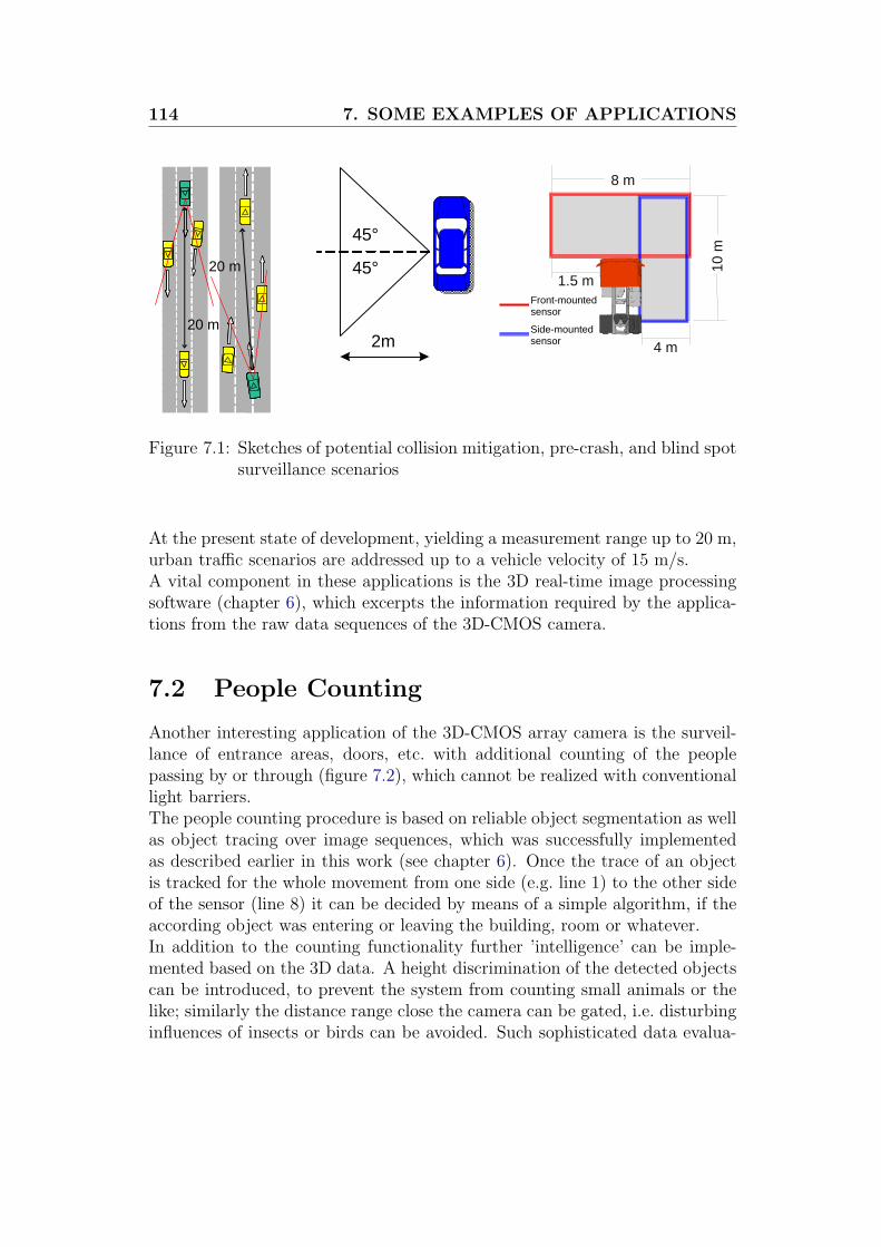
114 7. SOME EXAMPLES OF APPLICATIONS
20 m
20 m
8 m
4 m
1.5 mFront-mountedsensor
Side-mounted sensor
10 m
45°
45°
2m
Figure 7.1: Sketches of potential collision mitigation, pre-crash, and blind spotsurveillance scenarios
At the present state of development, yielding a measurement range up to 20 m,urban traffic scenarios are addressed up to a vehicle velocity of 15 m/s.A vital component in these applications is the 3D real-time image processingsoftware (chapter 6), which excerpts the information required by the applica-tions from the raw data sequences of the 3D-CMOS camera.
7.2 People Counting
Another interesting application of the 3D-CMOS array camera is the surveil-lance of entrance areas, doors, etc. with additional counting of the peoplepassing by or through (figure 7.2), which cannot be realized with conventionallight barriers.The people counting procedure is based on reliable object segmentation as wellas object tracing over image sequences, which was successfully implementedas described earlier in this work (see chapter 6). Once the trace of an objectis tracked for the whole movement from one side (e.g. line 1) to the other sideof the sensor (line 8) it can be decided by means of a simple algorithm, if theaccording object was entering or leaving the building, room or whatever.In addition to the counting functionality further ’intelligence’ can be imple-mented based on the 3D data. A height discrimination of the detected objectscan be introduced, to prevent the system from counting small animals or thelike; similarly the distance range close the camera can be gated, i.e. disturbinginfluences of insects or birds can be avoided. Such sophisticated data evalua-

7.3 Orientation Aid for Blind People 115
tion possibilities are not available when using conventional 2D-camera or lightbarrier systems.
Figure 7.2: People counting application
7.3 Orientation Aid for Blind People
In the CASBliP project [47], which aims at the development of a system capa-ble of interpreting and managing real world information from different sourcesto assist blind or visually impaired users, a portable 3D-CMOS sensor systemin the shape of eyeglasses is being presently developed. In combination witha space/audio processing unit which maps the distance information to specialsounds [48] the sensor should act as orientation aid for blind people (see figure7.3).A 64x1 pixel 3D-CMOS line sensor (one pixel line of a 64x4 pixel sensor [22]is used) is mounted together with the laser illumination unit and a circuitboard (including power supply, sensor control and raw data processing) in aeyeglasses-like housing and serves as device for the perception of the surround-ing. Sensor output of a single aquisition phase is a distance profile along theobserved line. Distance range of the system is from 0.5 m to 5 m with a rep-etition rate of 25 fps. Due to the position of the sensor system on the usershead, the environment is intuitively scanned by the head movements. Thegained distance data are then transferred to a main processing unit, where
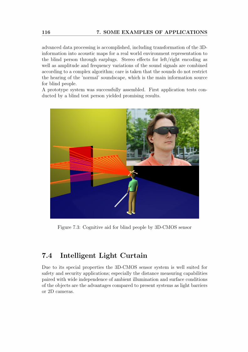
116 7. SOME EXAMPLES OF APPLICATIONS
advanced data processing is accomplished, including transformation of the 3D-information into acoustic maps for a real world environment representation tothe blind person through earplugs. Stereo effects for left/right encoding aswell as amplitude and frequency variations of the sound signals are combinedaccording to a complex algorithm; care is taken that the sounds do not restrictthe hearing of the ’normal’ soundscape, which is the main information sourcefor blind people.A prototype system was successfully assembled. First application tests con-ducted by a blind test person yielded promising results.
Figure 7.3: Cognitive aid for blind people by 3D-CMOS sensor
7.4 Intelligent Light Curtain
Due to its special properties the 3D-CMOS sensor system is well suited forsafety and security applications; especially the distance measuring capabilitiespaired with wide independence of ambient illumination and surface conditionsof the objects are the advantages compared to present systems as light barriersor 2D cameras.

7.4 Intelligent Light Curtain 117
Prototypes were assembled to demonstrate the capabilities of the systems asreflector-less intelligent light curtain. Special feature is here the structuredillumination that allows to cover a defined area with a light curtain (see figure7.4). Together with special compression optics, which images the illuminatedshape on a 64x1 pixel line sensor, curved light curtains can be realized. In thisway arbitrary surveillance fields can be realized.The distance information can here be used for definition of active and not ac-tive regions of the light curtain.
Figure 7.4: Intelligent light curtain
Many different applications can be envisioned for the intelligent light curtain.Some of them are:
• Object protection in museums (glassless show case)
• Area surveillance with possibility of defining active and non-active areas;e.g. a wall with doors and windows
• Intelligent light barrier for distances up to 100 m for small opening angles(invisible light fence), with exact localization of intrusion events by meansof the distance information

118 7. SOME EXAMPLES OF APPLICATIONS

Chapter 8
Conclusions and Further Work
This thesis is divided into two major parts. The first deals with the descriptionand evaluation of the newly developed 3D-CMOS camera system, the secondaddresses the image processing of the data acquired with the aforesaid camera.The following paragraphs give a conclusion of the results of the research donein these areas:
A novel 64x8 pixel range measurement system was successfully developed andassembled. The system evaluation yielded good results for the basic systemparameters. A noise equivalent exposure (NEE) of the sensor of 145 nJ/m2 ismeasured, the NEE of the over-all system results as 225 nJ/m2. Significantimprovement of the 64x8 pixel image sensor compared to the previous imagesensor generation is discovered in view of the rectangular shape of the shutterwindow function, which is crucial for good distance measurement results.Further we conclude that the perfomance of the developed camera systemagrees with the specified requirements (see chapter 1). Measurements showgood distance measurement linearity of the 3D-CMOS system and a distanceaccuracy lower than 3% of the measured distance over a distance range from2 m to over 20 m, for objects with surface reflectivities varying between 5%and 100% (Lambertian reflection). This means a dynamic range of the camerasystem in terms of radiant exposure of the sensor of over 96.5 dB.
The optimization of the distance measuring procedure showed that MDSI3,which was not applicable with the previous image sensor due to afore men-tioned insufficient shutter window properties, performs best with regard tomeasurement linearity, measurement accuracy, and measurement time. Thisresult was verified by calculations, simulations and experiments. Thus MDSI3has been taken as standard distance derivation algorithm for the camera sys-tem.

120 8. CONCLUSIONS AND FURTHER WORK
A further result of this work is a measurement technique that makes a gat-ing of the adverse signals, which come from raindrops or snowflakes in theclose range, possible; such a feature is indispensible for outdoor applications.Drawback is increased measurement noise due to the modified measurementmethod. Measurement results show the enhancements compared to a mea-surement without gating, but also reveal the shortcomings arising from thenon-ideal shutter window functions and laser-pulse shapes.
A main outcome of this thesis is the novel real-time image processing soft-ware, specifically developed for the image sequences of the 3D-CMOS camerasystem. It includes the segmentation, the tracking, and the classification ofobjects in the cameras volume of view (VOV).Highly robust object segmentation results as compared to the segmentationof 2D images could be achieved. The procedure is based on a suitable regiongrowing algorithm utilizing the distance information provided by the rangecamera.The newly developed tracking module showed preeminent performance as well.The object tracking is here accomplished by adaptive Kalman filtering, cus-tomized to the output data properties of the 3D CMOS sensor system withreal-time adaption to the scene properties. The filter tuning approach and thegood results of estimation of object positions, velocities and even accelerationsare demonstrated by means of example scenes.Based on the results of object segmentation and object tracking, object classi-fication and action prediction is performed. The basic concepts are describedin this work.
Finally we can conclude – as the measurement results in chapters 4 and 6show – that the 3D-CMOS array camera system in combination with the im-age processing software fulfills the application specific requirements. Thus thesystem development was successfully accomplished with promising results inview of future applications in the automotive and the safety sector.A deeper analysis of the performance of the camera system is presently exe-cuted at the UseRCams [1] project partners of the automotive industry, in-cluding BMW, FIAT, RENAULT, and VOLVO. They integrated the camerain test vehicles to evaluate the system in real traffic scenarios.

121
The work of this thesis could be extended by following further investigations:
Further investigations should address the crosstalk problem described in chap-ter 4.2.1.4. This could improve the 3D imaging capabilities of the system,especially for scenes with large reflectivity and/or distance dynamics.
Efforts should also be made to further decrease the noise and/or increase theresponsivity of the sensor. This could help to save laser diodes and reducetheir power, which presently are the most costly components of the camerasystem, or to increase the systems VOV.
The sensor could be improved with respect to alternating shutters during ana-log accumulation instead of the sequential shutters to reduce corruption ofmeasurement values on the edges of moving objects.
Efforts should be made to increase the pulse repetition rate of the laser lightsource. This would increase the frame repetition rate and decrease the afore-said edge effects on moving objects, and thus significantly improve the imageacquisition and image processing results.
The object recovery algorithm could be enhanced by shape or size comparisonof the objects in addition to the presently considered Mahalanobis distancecriterion. Also the number of previous frames used for object recovery shouldbe increased from a single frame to make backtracking of object merging andsplitting possible.
The tracking procedure could be improved by implementing
- autocorrelated process noise to consider the high-grade temporal cor-relation of the process noise in reality
- adjustable level process noise that could adapt the process noise levelto the behavior of the observed object
- multiple model tracking with model switching to adapt the processmodel and the state vector dimensions to the properties of the observedobject.
These improvement approaches are closely described in [42].
For improvement of the object classification capabilities of the 3D imaging sys-tem an increase of the sensor resolution and/or a combined image processingincluding high resolution 2D-images of the observed scene should be addressed.Efforts are already undertaken in the research project MIDIAS [46].

122 8. CONCLUSIONS AND FURTHER WORK

Appendix A
Basic Signals
A.1 The Rectangular Impulse
The standardized rectangular impulse is defined as
rect(t) =
1 , | t |≤ 1
2
0 , | t |> 12
for t ∈ R. (A.1)
Scaling by T and shifting by τ in direction of the t-axis leads to the generaldescription of a rectangular signal:
rect(t, T, τ) = rect
(t− τ
T
)=
1 , | t−τ
T|≤ 1
2
0 , | t−τT|> 1
2
(A.2)
A.2 The Dirac Impulse (Dirac δ-function)
The Dirac δ-function is defined by
δ(t) =
∞ , t = 0
0 , t 6= 0
mit t ∈ R (A.3)

124 A. BASIC SIGNALS
and ∫ ∞
−∞δ(t)dt = 1 . (A.4)
It is appropriate to describe the sampling of signals, as the integral over theproduct of a function f(t) with δ(t− τ) yields the sampled value f(τ) of f(t):
f(τ) =
∫ ∞
−∞f(t) · δ(t− τ)dt (A.5)

Appendix B
Random Variables
B.1 Probability Density Function (PDF)
For derivation of the pdf of a discrete random variable x, which can take thevalues in the set (ξi, i = 1, ..., n), firstly the probability mass function (pmf) isintroduced:
µx(ξi) = P (x = ξi) i = 1, ..., n (B.1)
with µi beeing the point masses.By means of the Dirac impulse function (cf. chapter A.2) the discrete pdfresults as
px(ξi) =N∑
i=1
µi · δ(x− ξi) . (B.2)
B.2 Gaussian Distribution
A continuously distributed random variable x is called Gaussian distributed[25], if its values are distributed according to equation B.3:
fx(ξ) =1√
2πσ2· e−
(ξ−µ)2
2σ2 (B.3)
Its probability density function pdf(x) looks like shown in figure B.1. The twoparameter µ and σ define the shape of the resulting distribution. Thereby isµ the offset of the function in ξ-direction; σ is a spread factor of the functionwith µ beeing the center of the spread.A short notation equivalent to B.3 is
pdf(x) ∼ (µ, σ2)

126 B. RANDOM VARIABLES
ξ
pdf (x) = fx(ξ)
σ
µ
Figure B.1: Gaussian distributed probability density function
For a Gaussian distribution fx(ξ) of a random variable x one can keep in mindtable B.1 which displays the portions of all drawn values x lying within aninterval µ− n · σ ≤ x ≤ µ+ n · σ for different values of n.
Table B.1: Portion of x-values contained in the µ± n · σ-interval
Interval Portion
µ− 1 · σ ≤ x ≤ µ+ 1 · σ 0.683
µ− 2 · σ ≤ x ≤ µ+ 2 · σ 0.954
µ− 3 · σ ≤ x ≤ µ+ 3 · σ 0.997
These numbers count for large numbers of draws, and must be seen as approx-imate values for small numbers.

Appendix C
Line Fitting
For a given set of N observations consisting of the xi- and yi-value vectors xand y, the line
yf = m · x+ b (C.1)
with
m =x · y − x · yx2 − (x)2
(C.2)
and
b =x2 · y − x · x · y
x2 − (x)2(C.3)
minimizes the quadratic error sum
N∑i=1
(yi − (m · xi + b))2 . (C.4)
The intersection of the fitted line with the x-axis
x|yf=0 = x0 =−bm
(C.5)
results from the above derived parameters as
x0 =x · x · y − x2 · y
x · y − x · y. (C.6)
This can also be expressed as
x0 =
−N−1∑i=1
[N∑
j=i+1
((yi − (yi−yj)
(xi−xj)· xj
)· (i− j)2
)]N−1∑i=1
[N∑
j=i+1
((yi−yj)
(xi−xj)· (i− j)2
)] (C.7)

128 C. LINE FITTING
which is actually a weighted mean of all possible combinations of two datapoints, and thus a weighted mean of all possible MDSI3 (see chapter 3.4) dis-tance calculations.
For accuracy calculation of the DCSI distance measuring method in chapter5.1.1 the partial derivative ∂x0
∂yiof x0 is required. It is computed according to
following equation:
∂x0
∂yi
=(x · y − x · y) · (x · xi
N− x2 · 1
N)− (x · x · y − x2 · y) · (x · xi
N− x · 1
N)
(x · y − x · y)2
(C.8)

Bibliography
[1] Ertico, “PReVENT project homepage,” http://www.prevent-ip.org/, sta-tus: 06/01/2007.
[2] P. Mengel and R. Wertheimer et al., “D52.300.1 camera re-quirements and specifications,” UseRCams project deliverable, avail-able from http://www.prevent-ip.org/en/public documents/deliverables/d523001 usercams general specifications.htm, status: 06/01/2007.
[3] Rudolf Millner, Ultraschalltechnik: Grundlagen und Anwendungen,Physik-Verlag, Weinheim, Germany, 1987.
[4] Erich Pehl, Mikrowellen in der Anwendung, Huthig, Heidelberg, Germany,1993.
[5] Bernd Jahne, Digital Image Processing, Springer, Berlin, Germany, 2005.
[6] F. Forster, Real-Time Range Imaging for Human-Machine Interface,Ph.D. thesis, Technische Universitat Munchen, 2005.
[7] D. Modrow et al., “3D face scanning systems based on invisible infraredcoded light,” in Proceedings ISVC07, Lake Tahoe, USA, Nov. 2007.
[8] S. Hsu et al., “Performance of a time-of-flight range camera for intelli-gent vehicle safety applications,” in Advanced Microsystems for Automo-tive Applicatioons 2006, J. Valldorf and W. Gessner, Eds., pp. 205–219.Springer, Berlin, Germany, 2006.
[9] R. Lange, 3D Time-of-Flight Distance Measurement with Custom Solid-State Image Sensors in CMOS/CCD-Technology, Ph.D. thesis, Univer-sitat Siegen, 2000.
[10] T. Oggier et al., “3D-imaging in real-time with miniturized optical rangecamera,” in Proceedings Opto-Conference, Nurnberg, Germany, 2004.

130 BIBLIOGRAPHY
[11] T. Oggier et al., “Novel pixel architecture with inherent background sup-pression for 3D time-of-flight imaging,” in Proceedings SPIE-IS&T, SanJose, USA, 2005, vol. 5665.
[12] C. Niclass et al., “A single photon detector array with 64x64 resolutionand millimetric depth accuracy for 3D imaging,” in Proceedings ISSCC,2005, pp. 364–365.
[13] M. Spies and H. Spies, “Automobile Lidar Sensorik: Stand, Trends undzukunftige Herausforderungen,” Advances in Radio Science, vol. 4, pp.99–104, 2006.
[14] K. Furstenberg and R. Schulz, “Laserscanner for driver assistance,” inProceedings WIT, Hamburg, Germany, 2006.
[15] G. Doemens P. Mengel and L. Listl, “Fast range imaging by CMOS sen-sor array through multiple double short time integration (MDSI),” inProceedings ICIP, Thessaloniki, Greece, Oct. 2001, vol. 2, pp. 333–336.
[16] D. Stoppa et al., “A 16x16-pixel range-finding CMOS image sensor,” inProceedings ESSCIRC, Leuven, Belgium, Sept. 2004, pp. 419–422.
[17] Graham Saxby, The Science of Imaging, Institute of Physics Publishing,Bristol, England, 2002.
[18] R. Kuhla, Hardware-Modellierung und Algorithmus-Optimierung furdie dreidimensionale Objekterfassung durch CMOS-Bildsensoren mitKurzzeitintegration und Laserpulsbeleuchtung, Ph.D. thesis, UniversitatDuisburg-Essen, 2007.
[19] Peter Gulden and Marc Fischer, “Verschiedene halbleiterbasierte Ver-fahren zur Bestimmung der Objektentfernung mit Hilfe der Lichtlaufzeit,”Sept. 2003, Internal research report Siemens AG.
[20] P. Mengel et al., “Three-dimensional CMOS image sensor for pedestrianprotection and collision mitigation,” in Advanced Microsystems for Auto-motive Applications 2006, J. Valldorf and W. Gessner, Eds., pp. 23–39.Springer, Berlin, Germany, 2006.
[21] P. Mengel et al., “Time-of-flight camera for pedestrian protection andcollision mitigation,” in Proceedings ITS, Aalborg, Denmark, June 2007.
[22] O. M. Schrey et al., “A 4x64 pixel CMOS image sensor for 3D mea-surement applications,” in Proceedings ESSCIRC, Estoril, Portugal, Sept.2003, pp. 169–172.

BIBLIOGRAPHY 131
[23] O. Elkhalili et al., “A 64x8 pixel 3-D CMOS time of flight image sensor forcar safety applications,” in Proceedings ESSCIRC, Montreux, Switzerland,Sept. 2006.
[24] FEMTO Messtechnik GmbH, “Photoreceiver HSA-Y-S,” informationavailable from http://www.femto.de, status: 06/01/2007.
[25] Lennart Rade and Bertil Westergren, Springers Mathematische Formeln,Springer, Berlin, Germany, 2nd edition, 1997.
[26] Eli Kapon, Semiconductor Lasers I, Academic Press, San Diego, USA,1998.
[27] “Communication with LEWICKI microelectronic GmbH,” informationavailable from http://www.lewicki.de, status: 06/01/2007.
[28] Normenstelle Informationstechnik im DIN Deutsches Institut fur Nor-mung e.V., “DIN EN 60825-1:2003-10 - Sicherheit von Lasereinrichtun-gen - Teil 1: Klassifizierung von Anlagen, Anforderungen und Benutzer-Richtlinien,” 2003.
[29] G. Hauske, “Statistische Signaltheorie,” Skriptum zur Vorlesung,Lehrstuhl fur Nachrichtentechnik, Technische Universitat Munchen, 2003.
[30] O. Elkhalili, Entwicklung von optischen 3D CMOS-Bildsensoren auf derBasis der Pulslaufzeitmessung, Ph.D. thesis, Universitat Duisburg-Essen,2004.
[31] B. Koenig, B. Hosticka, P. Mengel, and L. Listl, “Novel long distancecamera system with real-time 3D Image processing,” in Proceedings SPIEOptics & Photonics, San Diego, USA, Aug. 2007.
[32] E. Steinbach, “Medientechnik,” Skriptum zur Vorlesung, Lehrstuhl furKommunikationsnetze, Technische Universitat Munchen, 2002.
[33] Normenstelle Luftfahrt im DIN Deutsches Institut fur Normung e.V.,“DIN 9300 - Begriffe Großen und Formelzeichen der Flugmechanik,” 1990.
[34] David A. Forsyth and Jean Ponce, Computer Vision: A Modern Approach,Prentice Hall, Upper Saddle River, USA, 2003.
[35] Dana H. Ballard and Christopher M. Brown, Computer Vision, PrenticeHall, Englewood Cliffs, USA, 1986.
[36] Kenneth R. Castleman, Digital Image Processing, Prentice Hall, UpperSaddle River, USA, 1996.

132 BIBLIOGRAPHY
[37] A. Yilmaz, O. Javed, and M. Shah, “Object tracking: A survey,” ACMComput. Surv., vol. 38, no. 4, Dec. 2006, Article 13.
[38] Samual Blackman and Robert Popoli, Modern Tracking Systems, ArtechHouse, Boston, USA, 1999.
[39] R. E. Kalman, “A new approach to linear filtering and prediction prob-lems,” Transaction of the ASME-Journal of Basic Engineering, pp. 35–45,Mar. 1960.
[40] Peter Maybeck, Stochastic Models, Estimation, and Control, AcademicPress, San Diego, USA, 1979.
[41] G. Welch and G. Bishop, “An introduction to the Kalman filter,”http://www.cs.unc.edu/˜welch/kalman/, status: 06/01/2007.
[42] Yaakov Bar-Shalom and Xiao-Rong Li, Estimation and Tracking: Prin-ciples, Techniques, and Software, Artech House, Boston, USA, 1993.
[43] Robert Grover Brown and Patrick Y. C. Hwang, Introduction to RandomSignals and Applied Kalman Filtering, John Wiley & Sons, New York,USA, 3rd edition, 1997.
[44] Brian D.O. Anderson and John B. Moore, Optimal Filtering, DoverPublications, Mineola, USA, 2005.
[45] Elliott Kaplan, Understanding GPS: Principles and Applications, ArtechHouse, Boston, USA, 1996.
[46] FORWISS Passau, “MIDIAS project description,” http://www.forwiss.uni-passau.de/de/projectsingle/61/main.html, status: 07/01/2007.
[47] GITG Universidad Politecnica de Valencia, “CASBliP project homepage,”http://www.casblip.upv.es/, status: 07/01/2007.
[48] A. F. Rodrıguez Hernandez et al., “Figure perception from real and virtualsounding surfaces,” in Proceedings Technology and Persons with Disabili-ties Conference, Los Angeles, USA, 2003.
[49] EMVA European Machine Vision Association, “EMVA Standard 1288 -standard for characterization and presentation of specification data forimage sensors and cameras,” Aug. 2005, Release A1.00.

List of Abbreviations
2D 2-Dimensional3D 3-Dimensional3D-CMOS Acronym for the sensor chip technologyADC Analog to Digital ConverterAMSE Average Mean Square ErrorCCT Color Coded TriangulationCDS Correlated Double SamplingCMOS Complementary Metal Oxide SemiconductorCS Coordinate SystemCSI Correlated Short-time IntegrationCW Continuous waveDCSI Difference Correlated Short-time IntegrationDR Dynamic RangeFF Fill FactorFOV Field Of ViewFPGA Field Programmable Gate ArrayFPN Fixed Pattern NoiseFR Frame RateIR Infra-RedLASER Light Amplification by Stimulated Emission of RadiationLED Light Emitting DiodeLIDAR LIght Detection And RangingMDSI Multiple Double Short-time TntegrationMPE Maximum Permissible ExposureMSE Mean Square ErrorNEE Noise Equivalent ExposureNIR Near Infra-RedOL Object ListOTA Operational Transconductance AmplifierPD Photo DiodePDF Probability Density FunctionPRF Pulse Repetition Frequency

134 List of Abbrevations
RADAR RAdio Detection And RangingSF Source FollowerSNR Signal-to-Noise RatioSONAR SOund Navigation Rnd RangingTOF Time Of FlightVOV Volume Of ViewVRU Vulnerable Road User

List of Important Symbols
A state transition matrixAIll illuminated areaAObject object areaAPixel active pixel areaASensor active sensor areaAMSE average mean square errorC capacitanceCacc readout capacitanceCD diode capacitanceCH hold capacitanceCInt integrator capacitanceCsense sense capacitanceD aperture diameterDR dynamic rangeE irradianceESensor(t) irradiance characteristic on the sensor surface (from active illumination)EBack(t) background light irradiance characteristic on the sensor surfaceF camera focusFR camera frame rateH measurement matrixH radiant exposureI identity matrixID photo diode currentK Kalman gain matrixM magnification factor, shutter switchMSE mean square errorN number variableNEE noise equivalent exposureP estimate error covariance matrixPDiode incident power on the reference diodePModule output power of a laser modulePLaser(t) ideal laser pulse function

136 List of Symbols
PL laser pulse amplitudePRF pulse repetition frequencyQ process noise covariance matrixQphoto photo chargeR measurement noise covariance matrixRλ sensor responsivity for a given wavelength λSλSensor sensor sensitivity for a given wavelength λSλSensor(t) ideal shutter window functio for a given wavelength λ
SλS sensor sensitivity amplitude for a given wavelength λT discrete time periodTDL delay time of the laser pulseTDS delay time of the shutter windowTInt integration timeTPw pulse widthUCout ideal pixel output voltageUi ideal sensor output signal for shutter pulse alignment i, i ∈ a, b, c, dUInt integrator output voltageUDiode reference diode output voltageUddpix reference voltageUSensor ideal sensor output voltage
aE Euclidean distanceaM Mahalanobis distanceb basis lengthc speed of lightd distancedm measured target distancedr real target distanced(nacc) damping functionf focal length, frequencygSF amplification factor of the source followerf# f-numberk discrete time step instancenacc number of analog accumulationsnav number of averaged framesp disparityri residual of varaible irblur radius of a blur disct timetacqu acquisition timetTr laser trigger length

List of Symbols 137
u object distance, horizontal pixel indexuSensor sensor output voltagev measurement noise vectorv image distance, vertical pixel indexw process noise vectorx distance value in x-coordinate directionx system state vectory distance value in y-coordinate directionz distance value in z-coordinate directionz measurement vector
∆ difference operatorΦi digital control signal i
α angle variableβ angle variableθ angle variableκ optical loss factorλ wavelengthµi mean value of signal iρ surface reflectivityσi standard deviation of signal iσR readout noiseσS sensor noiseσU over-all system noiseσ∗U bright noiseτTOF time of flightφ angle variableψ angle variable

138 List of Symbols

List of Figures
1.1 UseRCams covered areas . . . . . . . . . . . . . . . . . . . . . . 2
2.1 Non-contact distance measurement methods . . . . . . . . . . . 62.2 Principle of time of flight measurements . . . . . . . . . . . . . 72.3 Michelson interferometer . . . . . . . . . . . . . . . . . . . . . . 82.4 Principles of stereo vision and active triangulation . . . . . . . . 92.5 Principle of continuous wave time of flight distance measure-
ment according to [8] . . . . . . . . . . . . . . . . . . . . . . . . 12
3.1 3D-CMOS measuring principle . . . . . . . . . . . . . . . . . . . 153.2 Imaging geometry . . . . . . . . . . . . . . . . . . . . . . . . . . 163.3 Ideal laser-pulse function . . . . . . . . . . . . . . . . . . . . . . 183.4 Ideal sensor sensitivity function . . . . . . . . . . . . . . . . . . 203.5 Ideal integrator output function for variation of the laser pulse
delay . . . . . . . . . . . . . . . . . . . . . . . . . . . . . . . . . 213.6 Possible alignments of a shutter window relatively to the inci-
dent light pulse . . . . . . . . . . . . . . . . . . . . . . . . . . . 233.7 Alignment of a shutter window relatively to the incident light
pulse at the gradient method . . . . . . . . . . . . . . . . . . . . 253.8 Example for the temporal alignment of laser pulses and shutter
windows at the CSI method . . . . . . . . . . . . . . . . . . . . 273.9 Distance measurement principle of the DCSI method . . . . . . 28
4.1 3D-CMOS array sensor system . . . . . . . . . . . . . . . . . . . 294.2 64x8 pixel 3D CMOS sensor . . . . . . . . . . . . . . . . . . . . 314.3 Pixel circuit with CDS readout stage [23] . . . . . . . . . . . . . 324.4 Simplified sensor timing [22] . . . . . . . . . . . . . . . . . . . . 324.5 Analog accumulation principle . . . . . . . . . . . . . . . . . . . 344.6 Sensor responsivity measurement at λ = 905 nm . . . . . . . . . 404.7 Sampled shutter window function for different shutter lengths tsh 414.8 Damping of the output signal increase during analog accumulation 424.9 Laser module output pulse shape . . . . . . . . . . . . . . . . . 45

140 LIST OF FIGURES
4.10 Evaluation of the PRF dependency of the laser module outputpower long-term characteristics . . . . . . . . . . . . . . . . . . 46
4.11 Fulfillment of laser class 1 regulations for different observationdistances . . . . . . . . . . . . . . . . . . . . . . . . . . . . . . . 48
4.12 Sources of the system noise . . . . . . . . . . . . . . . . . . . . 494.13 System dark noise mean values original and inversely damped . 514.14 PDF of the dark noise values . . . . . . . . . . . . . . . . . . . . 514.15 σU value of the sensor outputs for different sensor signal ampli-
tudes . . . . . . . . . . . . . . . . . . . . . . . . . . . . . . . . . 534.16 Determination of the NEE by extrapolating the fitted sensor
responsivity curve of figure 4.6 . . . . . . . . . . . . . . . . . . . 544.17 Shutter-window-pulse correlation investigations . . . . . . . . . 554.18 Accuracy of the measured distance dm for different targets and
camera parametrizations over a measurement range from 2 mto 20 m; the according nacc is added to each data point . . . . . 59
4.19 Distance measurement performance using MDSI3 algorithm andadaptive accumulation . . . . . . . . . . . . . . . . . . . . . . . 60
4.20 Fixed pattern noise of the sensor chip for 16 analog accumula-tions and a shutter length of 240 ns . . . . . . . . . . . . . . . . 62
4.21 Example of a distance calibration measurement curve for 16analog accumulations . . . . . . . . . . . . . . . . . . . . . . . . 63
5.1 Calculation of the expected distance measurement accuracy ac-cording to equations 5.4-5.10 . . . . . . . . . . . . . . . . . . . . 69
5.2 Simulation of the expected distance measurement accuracy forMDSI1, MDSI3 and DCSI . . . . . . . . . . . . . . . . . . . . . 70
5.3 Experimental comparison of the distance measurements for MDSI1and MDSI3 (ρ ∼50%) . . . . . . . . . . . . . . . . . . . . . . . . 71
5.4 Comparison of the measurement result and the calculation resultfor the ratio of the errors of MDSI1 and MDSI3 . . . . . . . . . 71
5.5 Radiant power on the sensor surface resulting from a raindropresp. a Lambertian reflecting object . . . . . . . . . . . . . . . . 74
5.6 Measured distance for a object with reflectivity ρ = 0.1 with asingle raindrop in the VOV at different distances . . . . . . . . . 74
5.7 Alignment of a shutter windows relatively to the incident lightpulse at the gradient method with gating of the close-up range . 76
5.8 Distance measurement results for different gating times TG fora target at 5 m and a glass bead at 0.5 m distance . . . . . . . . 76
6.1 Image processing chain . . . . . . . . . . . . . . . . . . . . . . . 796.2 Pixel and sensor coordinate systems . . . . . . . . . . . . . . . . 816.3 Sensor, camera, and world coordinate systems . . . . . . . . . . 82

LIST OF FIGURES 141
6.4 Structure of the object list of an image frame . . . . . . . . . . 866.5 Segmentation examples of synthetic and real depth images . . . 886.6 Series of consecutive object lists for the (k−1)-th, the k-th, and
the (k + 1)-th time step . . . . . . . . . . . . . . . . . . . . . . 906.7 Example ellipsoid of constant Mahalanobis distance . . . . . . . 916.8 Kalman filter principle . . . . . . . . . . . . . . . . . . . . . . . 956.9 Kalman filter formulas . . . . . . . . . . . . . . . . . . . . . . . 966.10 Synthetically produced camera frames . . . . . . . . . . . . . . 1026.11 Comparison of the distance measurement inaccuracy of real and
synthetic camera data . . . . . . . . . . . . . . . . . . . . . . . 1026.12 Synthetically produced example scenarios . . . . . . . . . . . . . 1046.13 Tracking results in x-direction for the synthetic car breaking
scenario for different values of σwx . . . . . . . . . . . . . . . . . 1056.14 Residual error and standard deviation of the tracking results of
figure 6.13 . . . . . . . . . . . . . . . . . . . . . . . . . . . . . . 1066.15 Determination of the optimal process noise value by minimizing
the average normalized error of x, x, and x . . . . . . . . . . . . 1086.16 Determination of the optimal measurement noise value in y-
direction by minimizing the average error of y, y and y . . . . . 1086.17 Real example scenario . . . . . . . . . . . . . . . . . . . . . . . 1096.18 Results of the tracking of a moving person . . . . . . . . . . . . 110
7.1 Sketches of potential collision mitigation, pre-crash, and blindspot surveillance scenarios . . . . . . . . . . . . . . . . . . . . . 114
7.2 People counting application . . . . . . . . . . . . . . . . . . . . 1157.3 Cognitive aid for blind people by 3D-CMOS sensor . . . . . . . 1167.4 Intelligent light curtain . . . . . . . . . . . . . . . . . . . . . . . 117
B.1 Gaussian distributed probability density function . . . . . . . . 126

142 LIST OF FIGURES

List of Tables
4.1 Properties of the customized imaging lenses . . . . . . . . . . . 37
6.1 Main parameter of the description format for segmented objects 876.2 Component noise contributions σpc for σφ � 1 and σθ � 1 . . . 99
B.1 Portion of x-values contained in the µ± n · σ-interval . . . . . . 126

144 LIST OF TABLES
![Tyson’s Corner • Bethesda Fhg]Zr](https://static.fdocuments.net/doc/165x107/606aa5af8b89964d9d2fbe06/tysonas-corner-a-bethesda-fhgzr-.jpg)


![= heh]bcg Fhg]he:elZc l'k'e - Geology · Fhg]he Q_obcgo»]`ebcgoZflugZ`beeZ]ZZguo¯jwwg^ Fhg]heMekZ^owjw]`¯¯e`[mcl»ke¯¯^bc]Zcf]ZZjgvoZjmmeZ\ …](https://static.fdocuments.net/doc/165x107/5e5e8a54f962267dfa24ff01/-hehbcg-fhgheelzc-lke-fhghe-qobcgoebcgozflugzbeezzzguojwwg-fhghemekzowjwemclkebczcfzzjgvozjmmez.jpg)


