OPTIMISATION OF WAISTED TENSILE TEST SPECIMEN …

A thesis submitted in partial fulfilment of the requirements for the degree of

Doctor of Philosophy

OPTIMISATION OF WAISTED TENSILE TEST SPECIMEN GEOMETRY AND DETERMINATION OF TENSILE ENERGY WELDING FACTORS FOR DIFFERENT POLYETHYLENE PIPE WALL THICKNESSES

MOHAMMAD TAGHIPOURFARD College of Engineering, Design and Physical Sciences

I

Abstract

High-density polyethylene (HDPE) pipes are employed in a wide range of industries such as water, gas,

nuclear and energy. HDPE pipes have steadily replaced clay, copper, asbestos-cement, aluminium, iron

and concrete pipes in various applications. Butt fusion welding is one of the most commonly used

techniques to weld HDPE pipes. There are many test methods available for assessing the short-term

performance of butt fusion welded joints in HDPE pipes. Recent research publications have shown

that waisted tensile test specimen is the most discriminating short-term examination in a tensile test,

such as those described in ISO 13953, EN 12814-2, EN 12814-7 and WIS 4-32-08.

The current challenge of using the abovementioned standards is to quantify the quality of welds since

the same waisted geometry is used for any pipe size diameter with any thickness. As the thickness of

the specimen increases, the degree of ductility reduces significantly in both welded and unwelded

specimens. Therefore, a new specimen geometry that can be used for specimens with all thicknesses

must be defined to allow a more accurate measurement of weld quality.

In order to simplify the aforementioned problem, specimens using an unwelded flat sheet made from

HDPE were used to investigate the geometry parameters, which believed to have the most influence

on the fracture of the specimen. The effects of parameters such as width and radius of the waisted

section, diameter and distance of loading holes, and overall width of the specimen were investigated

through various experimental procedures, tensile tests, and Central Composite Design (CCD)

optimisation.

After understanding the effect of geometry parameters, Finite Element Analysis (FEA) techniques

using constitutive equations are used to confirm experimental findings. FEA modelling also covered a

wide range of specimen geometries, where the experimental investigation was not feasible due to

machining and testing limitations of specimens with large thicknesses (e.g., 20-100mm).

The final contribution of this thesis is to propose a modified geometry, which could be used for all pipe

sizes and demonstrate its advantages over the standard geometry specimen. This task was carried out

on pipes with Outer Diameter (OD) of 140, 160, 250, 280, 500 and 630mm. Improvements on 140, 160

and 250mm with a thickness of less than 20mm, are providing more considerable elongation using

parent pipe material and necking starting at earlier stages of the tensile test. Improvements on 280,

500 and 630mm OD with a thickness of over 20mm, are having the specimen fail in a ductile manner

with ductility in welded and unwelded specimen whereas, no ductility could be observed when

standard geometry was used. X-ray photography was taken to verify the types of failures accrued in

specimens. The outcome of the research conducted in this thesis, which proposed a modified

geometry for tensile tests, paves the way to enhance reliability in the examination of HDPE weld

qualities.

II

Table of Contents

Abstract ................................................................................................................................. I

List of Figures ..................................................................................................................... VIII

List of Tables ...................................................................................................................... XIX

List of Abbreviations .......................................................................................................... XXI

List of Symbols ................................................................................................................. XXIII

Statement of original Authorship ...................................................................................... XXV

Acknowledgments ........................................................................................................... XXVI

Chapter 1. Introduction ...................................................................................................... 1

Industrial needs ................................................................................................................... 3

Aim and Objectives .............................................................................................................. 4

Thesis Structure ................................................................................................................... 5

Chapter 2. Background Theory ........................................................................................... 7

Chapter Overview ................................................................................................................ 7

2.1.1 Introduction to Polymers ................................................................................................. 7

2.1.2 Polymer Types ................................................................................................................. 7

2.1.3 Polymerisation ................................................................................................................. 9

2.1.4 Amorphous and Semi-Crystalline Thermoplastics, .......................................................... 10

2.1.5 Polymer Molecular weight ............................................................................................. 11

2.1.6 Polyethylene .................................................................................................................. 12

III

PE Pipes and Applications .................................................................................................. 13

2.2.1 PE Pipe Manufacturing ................................................................................................... 14

2.2.2 Pipe Extrusion ................................................................................................................ 15

2.2.3 Classification .................................................................................................................. 18

Welding of Thermoplastics ................................................................................................ 19

2.3.1 Welding theory .............................................................................................................. 22

2.3.2 Hot Plate Welding .......................................................................................................... 23

The integrity of Plastic Joints ............................................................................................. 24

2.4.1 Safety-critical applications.............................................................................................. 24

2.4.2 Different types of Defects .............................................................................................. 24

2.4.3 Modes of Failure ............................................................................................................ 25

Mechanical Testing ............................................................................................................ 27

2.5.1 Bend Tests ..................................................................................................................... 27

2.5.2 Short-Term Testing ........................................................................................................ 29

2.5.3 Tensile test using dumb-bell specimens ......................................................................... 30

2.5.4 Tensile test using waisted specimen ............................................................................... 32

2.5.5 Tensile Impact tests ....................................................................................................... 35

2.5.6 Hydrostatic pressure test ............................................................................................... 36

Mechanics of Materials ..................................................................................................... 38

2.6.1 Introduction ................................................................................................................... 38

IV

2.6.2 Stress Distribution at the Neck ....................................................................................... 38

2.6.3 Fracture in High-Density Polyethylene ............................................................................ 38

2.6.4 Fracture toughness range in high-density polyethylene .................................................. 42

2.6.5 Triaxiality ....................................................................................................................... 43

Summary ........................................................................................................................... 44

Chapter 3. Effect of the width of the waisted section on the properties of the waisted tensile

test specimen ..................................................................................................................... 45

Chapter overview .............................................................................................................. 45

Literature review ............................................................................................................... 45

Problem definition and research methodology .................................................................. 48

Experimental setup............................................................................................................ 49

Results and discussion ....................................................................................................... 51

Summary ........................................................................................................................... 64

Chapter 4. Effect of different parameters of waisted tensile test specimen using DOE

optimisation 65

Chapter Overview .............................................................................................................. 65

Literature review ............................................................................................................... 66

Experiment ........................................................................................................................ 68

4.3.1 The material, sample preparation, and testing ............................................................... 68

4.3.2 Design of experiment and characterisation .................................................................... 69

Results and Discussions ..................................................................................................... 71

V

4.4.1 Optimisation of Total Energy Factor ............................................................................... 72

4.4.2 Optimisation of Region 3 Energy Factor.......................................................................... 76

4.4.3 Optimisation for Loading Pin Holes Factor ...................................................................... 79

Maximisation and minimisation of the responses .............................................................. 81

Conclusion ......................................................................................................................... 84

Chapter 5. Modelling of necking in HDPE specimen and effect of triaxiality factor ............ 86

Chapter overview .............................................................................................................. 86

Literature Review .............................................................................................................. 86

Materials and experimental method .................................................................................. 88

5.3.1 Materials........................................................................................................................ 88

Numerical Study ................................................................................................................ 89

5.4.1 FEA Validation ................................................................................................................ 91

Results............................................................................................................................... 96

5.5.1 Effect of Specimen thickness .......................................................................................... 96

5.5.2 Effect of the width of the waisted section on triaxiality .................................................. 99

5.5.3 Effect of the radius of the waisted section on triaxiality ............................................... 102

5.5.4 Effect of the width of the waisted section and loading hole diameter on elongation in the

loading hole ............................................................................................................................... 103

5.5.5 Ductile and micro-ductile failure .................................................................................. 108

Conclusion ....................................................................................................................... 112

VI

Chapter 6. Proposed specimen geometry and its application on welded and unwelded HDPE

pipes…………….................................................................................................................... 114

Chapter overview ............................................................................................................ 114

Introduction .................................................................................................................... 114

Designed geometry for different thicknesses ................................................................... 115

Pipe Sizes ........................................................................................................................ 119

Butt Fusion Welding ........................................................................................................ 120

Pipe with 140mm outer diameter .................................................................................... 123






Comparison of Welding Factors ....................................................................................... 160

Conclusion ....................................................................................................................... 161

Chapter 7. Conclusions and future works ....................................................................... 162

Main findings of this thesis .............................................................................................. 162

Recommendations for future work .................................................................................. 165

Bibliography ...................................................................................................................... 166

Chapter 8. Appendix ...................................................................................................... 179

VII

Part A (Chapter 3) ............................................................................................................ 179

Part B (Chapter 4) ............................................................................................................ 181

Part C (Chapter 5) ............................................................................................................ 188

Part D (Chapter 6) ............................................................................................................ 192

VIII

List of Figures

Figure 1-1, Waisted tensile test specimen (EN12814-7) ......................................................... 1

Figure 1-2 Three different types of failures in a waisted tensile test. From left; brittle, mixed

and ductile failure ................................................................................................................. 2

Figure 2-1 Schematic diagram of the polymer structure [9] ................................................... 8

Figure 2-2 Reactions to the productions of polyethylene terephthalate [11] ....................... 10

Figure 2-3, Typical Extrusion Line [17] ................................................................................. 16

Figure 2-4 Single-Screw Extruder [18] .................................................................................. 17

Figure 2-5, Determination of bend angle and the ram displacement (BS EN 12814-1) ......... 28

Figure 2-6, Type 2 specimen geometry and dimensions (mm) (EN-12814-2) ........................ 32

Figure 2-7, Recommended Waisted tensile test specimen by WIS standard [46].................. 33

Figure 2-8 Notched tensile specimen geometry and dimensions [45] .................................. 33

Figure 2-9, Type A tensile test specimen for wall thickness less than 25mm (ISO 13953) ..... 34

Figure 2-10 Type B tensile test specimen for wall thickness greater than 25mm (ISO 13953)

........................................................................................................................................... 34

Figure 2-11, Tensile impact test specimen (all dimensions are in inches) (ASTM F2634) ...... 36

Figure 2-12, Dent Specimen with FPZ zone shown ............................................................... 42

IX

Figure 3-1. Dent Specimen with FPZ zone shown [48].......................................................... 48

Figure 3-2 from left ductile, brittle and mixed failure mode according to WIS 4-32-08 ........ 50

Figure 3-3, from left tensile testing with and without side plates ........................................ 50

Figure 3-4 Graph shows the total energy to break value per CSA against the width of the

waisted section for 15mm sheet thickness with side plates (Experiment 1) ......................... 52

Figure 3-5 Graph shows the force-displacement curve for specimen no PEW02, divided into

four regions ........................................................................................................................ 53

Figure 3-6, Energy to break values of different regions against the width of the waisted section

for the first experiment ....................................................................................................... 54

Figure 3-7, Load-displacement for 20mm and 40mm width of the waisted section.............. 55

Figure 3-8 Total energy to break value per CSA against the width of the waisted section for

25mm sheet thickness with side plates (experiment 2) ....................................................... 56

Figure 3-9, Force-displacement curve divided into two regions ........................................... 56

Figure 3-10, Total energy to break value per CSA against the width of the waisted section for

25mm sheet thickness with side plates (experiment 2) ....................................................... 58

Figure 3-11, Energy per CSA against the width of the waisted section on 15mm thick specimen

with and without side plates for Region 1 ........................................................................... 59



X





Figure 3-15, Load vs displacement for 15mm thick specimen with and without side plates . 62

Figure 3-16, Load-Displacement curve for 25mm thickness with 15mm to 27.5mm in width of

the waisted section (in order, from the smallest to largest graph, where 15mm is the smallest

and 27.5 is the largest) ........................................................................................................ 63

Figure 4-1: Waisted tensile test specimen (EN 12814-7) (dimensions in mm) ...................... 66

Figure 4-2: Central Composite Design (CCD) experimental space [77] .................................. 68

Figure 4-3: Example of a typical Force-Deformation graph .................................................. 71

Figure 4-4, Tensile tested specimens for the DOE experiment ............................................. 72

Figure 4-5: Total energy to break values per unit CSA .......................................................... 74

Figure 4-6: Main effect plot for total energy to break per unit CSA value for specific terms . 75

Figure 4-7: Region 3 energy to break values per unit CSA .................................................... 77

Figure 4-8: Main effect plot for Region 3 energy ................................................................. 78

Figure 4-9: Elongation in the loading pinhole ...................................................................... 80

Figure 4-10: Main effect plot for elongation in the loading pinhole. .................................... 81

XI

Figure 4-11, Desirability and parameters ............................................................................. 83

Figure 5-1, True stress-true strain graph for HDPE ............................................................... 90

Figure 5-2, Necking steps in the dumbbell test specimen .................................................... 91

Figure 5-3, Validation of the FEA model on a particular specimen with a thickness of 15mm,

the Loading hole diameter of 20mm and width of the waisted section of 17.5mm (refer to

figure 8-2 to figure 8-6 for the necking of the specimen) ..................................................... 92

Figure 5-4, Geometry configuration for determining the geometry effects on triaxiality ...... 93

Figure 5-5, Triaxiality measurement point locations in the specimens ................................. 94

Figure 5-6, Boundary conditions and fixed point for the geometry used .............................. 95

Figure 5-7, Mesh setting for the geometry used .................................................................. 95

Figure 5-8, Early increment of neck development modelling ............................................... 96

Figure 5-9, later increment of neck development modelling ................................................ 97

Figure 5-10, Variation of triaxiality across the width of the waisted section for specimens with

different thicknesses (width of the waisted section 25mm and radius of the waisted section

10mm) ................................................................................................................................ 98

Figure 5-11, Experimental Load-Displacement for 15 and 25mm thickness .......................... 99

Figure 5-12, Validation of across the width of the waisted section for specimens with different

widths of the waisted section (wall thickness 25mm, the radius of the waisted section 5mm)

......................................................................................................................................... 100

XII

Figure 5-13, Load-displacement curves on 25mm thick specimens varying the width of the

waisted section ................................................................................................................. 101

Figure 5-14, Variation of triaxiality across the width of the waisted section for specimens with

a different radius of the waisted section (width of the waisted section 25mm) ................. 103

Figure 5-15, Boundary conditions and meshing used for determining the effect of the width of

the waisted section on elongation in loading hole diameter .............................................. 104

Figure 5-16, Detailed mesh configuration at the wasited area ........................................... 105

Figure 5-17, Early increment of neck modelling using symmetry geometry........................ 106

Figure 5-18, Later increment of neck modelling using symmetry geometry ....................... 106

Figure 5-19, Elongation of the loading hole versus the deformation in the specimen for

different widths of the waisted section and constant loading hole diameter of 20mm (wall

thickness 30mm, the radius of waisted section 5mm) ....................................................... 107

Figure 5-20, Elongation of the loading hole versus deformation of the specimen for different

widths of the waisted section (wall thickness 30mm, the radius of waisted section 5mm,

loading hole diameter same as the width of the waisted section) ..................................... 108

Figure 5-21, Xray photography of micro ductile failure for specimen number 42 ............... 109

Figure 5-22, X-Ray Photography of micro ductile failure for specimen number 42 ............. 110

Figure 5-23, X-Ray photography of ductile failure for specimen no 37 ............................... 111

Figure 5-24, X-Ray photography of ductile failure for specimen no 37 ............................... 111

XIII

Figure 5-25, from left, fully ductile and micro ductile failure ............................................. 112

Figure 6-1, reduced section specimen related to the table below ...................................... 117

Figure 6-2, Schematic diagram of the pressure cycle during the butt fusion welding process)

......................................................................................................................................... 121

Figure 6-3, Modified geometry on the left used for thicknesses less than 20mm vs standard

12814-7 geometry on the right ......................................................................................... 124

Figure 6-4, Force-Deformation graph for modified and standard geometry on unwelded

140mm OD pipe ................................................................................................................ 125

Figure 6-5, Fracture surface of the parent standard on the left and parent modified geometry

on the right from 140mm OD pipe .................................................................................... 126

Figure 6-6, Nominal stress-Deformation graph for modified and standard geometry on

unwelded 140mm OD pipe ............................................................................................... 127

Figure 6-7, Nominal stress-Deformation graph for modified and standard geometry on welded

140mm OD pipe ................................................................................................................ 128

Figure 6-8, Fracture surface of welded standard specimen on the left and welded modified

specimen geometry on the right from 140mm OD pipe ..................................................... 128

Figure 6-9, From Left, fracture surface of standard, modified, standard and modified specimen

geometry from 140mm OD welded pipe ........................................................................... 129


welded with beads off on 140mm OD pipe........................................................................ 130

XIV

Figure 6-11, Fracture surface of the welded standard specimen on the left and welded

modified specimen geometry on the right from 140mm OD beads off pipe ....................... 130

Figure 6-12, Total Energy per CSA for different scenarios on 140mm OD SDR 11 pipe ....... 131


parent 160mm OD pipe..................................................................................................... 132

Figure 6-14, Nominal Stress-Deformation graph for modified and standard geometry on

welded 160mm OD pipe ................................................................................................... 133

Figure 6-15, Total Energy per CSA (mJ/mm2) for different scenarios on 160mm OD SDR 11 pipe

......................................................................................................................................... 134

Figure 6-16, Fracture surface of the welded modified specimen on the left and welded

standard specimen geometry on the right from 160mm OD pipe ...................................... 134


parent 250mm OD pipe..................................................................................................... 135

Figure 6-18, From left, fracture surface of standard, standard, modified and modified

specimen geometry on 250mm OD parent pipe ................................................................ 136


welded 250mm OD pipe ................................................................................................... 137


......................................................................................................................................... 137

XV

Figure 6-21, From left, fracture surface of modified, modified, modified, standard, standard

and standard specimen geometry on 250mm OD welded pipe .......................................... 138

Figure 6-22, from left to right, standard and modified geometry used for thickness in between

25mm and 30mm.............................................................................................................. 139


parent 280mm OD pipe..................................................................................................... 140


welded 280mm OD ........................................................................................................... 141

Figure 6-25, Fracture surface of the welded standard specimen on the left and modified

welded geometry on the right from welded 280mm OD pipe ............................................ 141

Figure 6-26, Total Energy per CSA (mJ/mm2) for different cases on 280mm OD SDR 11 pipe

......................................................................................................................................... 142

Figure 6-27, Fracture surface for welded 280mm OD pipe using standard and modified

geometry .......................................................................................................................... 143

Figure 6-28, Fracture surface of modified welded specimen from 280mm pipe (PEB195) .. 144

Figure 6-29, Fracture surface of standard welded specimen from 280mm pipe (PEB191) .. 145

Figure 6-30, From top left clockwise, Trimming, pipe position in the machine, heater plate in

place, final weld ................................................................................................................ 146


parent 500mm OD SDR 11 pipe ......................................................................................... 147

XVI


welded 500mm OD ........................................................................................................... 148


......................................................................................................................................... 149

Figure 6-34, Fracture surface for parent 500mm OD SDR 11 pipe using standard and modified

geometry .......................................................................................................................... 150

Figure 6-35, Fracture surface for parent modified specimen on the left (PEB204) and parent

standard specimen on the right (PEB197) from 500mm OD pipe ....................................... 151

Figure 6-36, Fracture surface for welded 500mm OD pipe SDR 11 using standard and modified

geometry .......................................................................................................................... 152

Figure 6-37, Fracture surface for welded modified specimen on the left (PEB213) and welded

standard specimen on the right (PEB206) from 500mm OD pipe and from the same weld 153


parent 630mm OD SDR11 pipe .......................................................................................... 154


welded 630m OD SDR11 pipe ............................................................................................ 155


......................................................................................................................................... 155

Figure 6-41, Fracture surface for parent 630mm OD pipe SDR11 using standard and modified

geometry .......................................................................................................................... 156

XVII

Figure 6-42, Fracture surface for parent 630mm OD pipe SDR 11 using standard on right and

modified geometry on the left .......................................................................................... 157

Figure 6-43, Fracture surface for welded 630mm OD pipe SDR 11 using standard and modified

geometry .......................................................................................................................... 158

Figure 6-44, Fracture surface for welded modified specimen on the left (PEB233) and welded

standard specimen on the right (PEB226) from 630mm OD pipe and from the same weld 159

Figure 6-45, Welding factors for different pipe sizes .......................................................... 160

Figure 8-1, Tensile test engineering design for DIC purpose............................................... 189

Figure 8-2, Initial increment and mesh for PEW36 specimen for FEA result Figure 5-3 ....... 189

Figure 8-3, Mesh configuration for the wasited area of specimen PEW36 for FEA result Figure

5-3 .................................................................................................................................... 190

Figure 8-4, Increment 7 for PEW36 specimen for FEA result in Figure 5-3 .......................... 190

Figure 8-5, Increment 26 for PEW 36 specimen for FEA result in Figure 5-3 ....................... 191

Figure 8-6, Increment 39 for PEW 36 for FEA result in Figure 5-3 ....................................... 191

Figure 8-7, Weld report for the first 500mm OD pipe weld ................................................ 200

Figure 8-8, Weld report for the second 500mm OD pipe ................................................... 201

Figure 8-9, Weld report for first 630mm OD pipe weld ...................................................... 202

Figure 8-10, Weld report for the second 630mm OD pipe weld ......................................... 203

XVIII

Figure 8-11, Weld reports for 250mm OD SDR17............................................................... 204



XIX

List of Tables

Table 2-1, Cell Classification System from ASTM D 3350-06 [19] .......................................... 18

Table 2-2 Code letter presentation (D3350) ........................................................................ 19

Table 2-3 Ram displacement corresponding to the bend angle of 160˚ ................................ 28

Table 2-4, Dimensions of the tensile test specimens in ISO 13953 ....................................... 35

Table 3-1, Set of Experiments carried out to investigate the effect of the waisted section ... 51

Table 4-1, Variables used in the central composite design ................................................... 70

Table 4-2, Optimisation results for predicted vs actual values ............................................. 84

Table 6-1, Dimensions for reduced section specimen geometry given in WIS 4-32-08:2-17 and

the proposed optimised geometry from this study ............................................................ 117

Table 6-2, Dimensions for BS EN 12814-7 standard and improved geometry ..................... 118

Table 6-3, Pipes used for this study with their dimensions and welding machines used ..... 119

Table 6-4, Recommended values for the heated tool butt welding of pipes (DVS-2207-01) 122

Table 8-1, Data for Experiment 1 (15mm thickness unwelded flat sheet with side plates) . 179

Table 8-2, Data for experiment 2 (25mm thickness, unwelded flat sheet with side plates) 179

Table 8-3, Data for Experiment 3 (15mm thickness, unwelded flat sheet).......................... 180

Table 8-4, Data for DOE analysis (15mm flat sheet specimen) ........................................... 181

XX

Table 8-5, ANOVA results for total energy response .......................................................... 184

Table 8-6, ANOVA results for Region 3 energy ................................................................... 185

Table 8-7, ANOVA results for elongation in loading pin holes ............................................ 187

Table 8-8, Constants used in constitutive equation ........................................................... 188

Table 8-9, data for 140mm OD pipes ................................................................................. 192

Table 8-10, Data for 160mm OD pipe ................................................................................ 193





Table 8-15, Data for all the weldings in this research ......................................................... 199

XXI

List of Abbreviations

ANN Artificial Neural Network

ANOVA Analysis of Variance

ASTM American Society for Testing and Materials

AWS American Welding Society

AWWA American Water Works associations

BS EN British Standard European Norm

CCD Central Composite Design

CSA Cross Sectional Area

CSA Canadian Standards Association

CTOD Crack Tip Opening Displacement

DIC Digital Image Correlation

DOE Design of Experiment

DP Degree of Polymerization

ESCR Environmental Stress Crack Resistance

EWF Essential Work of Fracture

FE Finite Element

FEA Finite Element Analysis

FPZ Fracture Process Zone

HDPE High-Density Polyethylene

ISO International Organization for Standardization

LB Larger Better

LEFM Linear Elastic Fracture Mechanic

XXII

MS Mean Square

MW Molecular Weight

NB Nominal Better

NLEFM Non-Linear Elastic Fracture Mechanic

OD Outer Diameter

PE Polyethylene

RSM Response Surface Methodology

SB Smaller Better

SCG Slow Crack Growth

SDR Ratio of Diameter to wall Thickness

SS Sum of Square

WIS water Industry Specification

XXIII

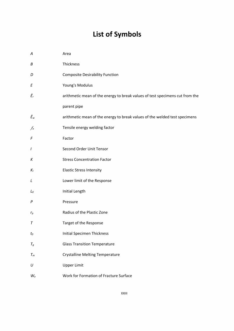
List of Symbols

A Area

B Thickness

D Composite Desirability Function

E Young's Modulus

Ēr arithmetic mean of the energy to break values of test specimens cut from the

parent pipe

Ēw arithmetic mean of the energy to break values of the welded test specimens

e Tensile energy welding factor

F Factor

I Second Order Unit Tensor

K Stress Concentration Factor

KI Elastic Stress Intensity

L Lower limit of the Response

L0 Initial Length

P Pressure

rp Radius of the Plastic Zone

T Target of the Response

t0 Initial Specimen Thickness

Tg Glass Transition Temperature

Tm Crystalline Melting Temperature

U Upper Limit

We Work for Formation of Fracture Surface

XXIV

wf Total Work of Fracture

Wp Work for Plastic Deformation

X Vector of the designed Variables

y Response

α f Final Angle

β Shape Factor

σ Average Stress

σ_r Radial Stress

σ_t Transverse Stress

σ1 First Principal Stress

σ2 Second Principal Stress

σ3 Third Principal Stress

σeqv Von-Mises Equivalent Stress

σh Hydrostatic Pressure Stress

𝑀𝑛 Number average

𝑀𝑤 Weight Average

ni Number of Molecules

Wi Weight

KIC Plane-Strain Fracture Toughness

σy Yield Stress

σ∗ Stress Triaxiality

XXV

Statement of original Authorship

The work contained in this thesis has not been previously submitted to the requirement for

an award at this or any other higher education institution. To the best of my knowledge and

belief, the thesis contains no material previously published or written by another person

except where due reference is made.

Signature:

Date:

XXVI

Acknowledgments

I would like to take this opportunity to thank everyone who helped me in different ways to achieve

this valuable milestone in my life.

First of all, I would like to thank my family, especially my younger brother Amir, for their love and

support throughout my life. Without you, I could have never got to this stage.

Special praise should be reserved for my industrial supervisor, Dr. Mike Troughton. Not only I have

gained technical knowledge from him throughout my PhD programme, I have learned how approach

and solve challenging problems. Mike, your contribution to this work cannot be overstated.

I would like to offer special thanks to Dr. Amir Khamsehnezhad and Steve Willis for their constant care,

guidance and supervision. They have always given me assurance and believed in the integrity of my

research work. I am also grateful to Prof. Jim Song, Dr. Bin Wang and Prof. Luis Wrobel for their

continuous support throughout the research.

I gratefully acknowledge my friends and colleagues within TWI and Brunel University London,

especially Dr. Sina Fateri for giving me guidance and motivation to finish this work and Dr. Mario

Kostan for making my life in Cambridge more enjoyable.

Finally I would like to thank the Engineering and Physical Sciences research Board (EPSRC), Brunel

University London and TWI for providing the funding for this research.

1

Chapter 1. Introduction

The first plastic pipes were installed in the mid-1930s, with their usage increasing rapidly in the 1950s.

Plastics have steadily replaced clay, copper, asbestos-cement, aluminium, iron and concrete pipes in

various applications. Polyethylene (PE) is employed in about 20% of plastic pipe applications [1, 2].

High-density polyethylene (HDPE) pipes are used extensively for the transportation and distribution

of natural gas, with over 80% of the new piping installations using HDPE.

There are many tests available for assessing the short-term performance of butt fusion welded joints

in HDPE pipes. Previous work [3, 4] has shown that the most discriminating short-term test is a tensile

test using waisted test specimen (Figure 1-1), such as those described in ISO 13953, EN 12814-2,

EN12814-7 and WIS 4-32-08.

Figure 1-1, Waisted tensile test specimen (EN12814-7)

2

This type of test is therefore specified in some standards relating to the qualification of butt fusion

welding procedures and welding operators for PE pipes (EN 13067, AWS B2.4).

In tensile tests using a waisted specimen [4], it is shown that the most discriminating test parameter

is the energy to break the specimen. Standards such as ISO 13953, EN 12814-2, EN 12814-6 and EN

12814-7 describe tensile tests on butt fusion welds in PE pipes where the Cross-Sectional Area (CSA)

is at minimum at the weld interface. Most of these tests specify that the tensile strength of the welded

specimen is determined and compared to that of a specimen cut from the parent pipe. However,

Chipperfield & Troughton [4] showed that tensile strength is a poor discriminator of weld quality. ISO

13953 specifies that the fracture surfaces of the tested specimen should be examined and categorised

as either ductile (large-scale deformation and yielding of material at the weld interface) or brittle (little

or no large-scale deformation of material at the weld interface). However, as can be seen in Figure 1-2

this categorisation is subjective, qualitative and the degree of ductility reduces significantly with wall

thickness [5].

Figure 1-2, Three different types of failures in a waisted tensile test. From left; brittle, mixed and ductile failure

3

EN 12814-7 does specify measuring the energy to break of the specimen and determining a tensile

energy welding factor, e, defined as:

𝑓𝑒 = 𝐸𝑤

𝐸𝑟 Equation 1-1

Where Ēw is the arithmetic mean of the energy to break values of the welded test specimens and Ēr is

the arithmetic mean of the energy to break values of test specimens cut from the parent pipe.

The values of energy to break have been shown to be dependent on wall thickness [6] and specimen

geometry [7] and may also be dependent on PE resin and butt fusion welding procedure.

Industrial needs

HDPE pipes are employed in a wide range of industries such as water, gas, nuclear, and energy. A

government review of the UK’s electrical energy requirements for 2025 has indicated that 60 GW of

net new capacity will be required to meet demand. This need comes from new nuclear fission

installations, which require joining of HDPE pipes. The implementation of these pipes in nuclear power

plants with strict policies, regulations, and inspection practices require a vote of confidence for

structural integrity and accurate prediction of welds’ lifetime. Currently, standard BS EN 12814-7 is

used to quantify between different qualities of welds. This standard fails to provide accurate

discrimination among different weld qualities, especially for pipes with large thicknesses (25mm and

above). Therefore, an updated specimen geometry is required to provide accurate testing methods

for the abovementioned industries.

4

Aim and Objectives

This research aims to investigate and improve the current standard geometry in quantifying the quality

of welds in HDPE pipes. Specific objectives of this research are:

• To investigate the current standard specimen geometry and identify factors indicating the

quality of the welds.

• To investigate the effect of geometry parameters on the value of the tensile energy to break

of welds experimentally.

• To determine the effect of specimen thickness on the failure of the waisted specimen via Finite

Element Analysis (FEA).

• To propose the most appropriate specimen geometry for tensile tests using waisted

specimens, which provides the most discrimination between different weld qualities.

• To provide a quantitative comparison between energy to break values of the standard and

proposed/improved geometry for pipes with different wall thicknesses and dimensions.

5

Thesis Structure

A combination of laboratory experiments, optimisation modelling, and FEA analysis are employed to

evaluate the effect of geometry parameters on specimen failure. This led to four distinct contributions

to knowledge which are listed below:

• The effect of the width of waisted section specimen on waisted geometry at 15 and 25mm

thickness using different test techniques are investigated. Total energy to break value of

specimen has been considered in recent literature as an indication of ductility in a specimen.

Therefore, specimen tensile tests have been compared against energy to break values. During

the observation of tensile tests, elongation around the loading hole could be observed;

therefore, in this research, different regions for the energy consumed are defined as the area

of interest (waisted area). Thus, Region 3 (energy consumed in necking of the specimen) is

proposed to be used as an indication of ductility in the waisted region. The most suitable width

of the waisted section, for a particular thickness, was found to have an aspect ratio of 1 to the

thickness.

• Optimisation modelling technique is employed to investigate five different parameters of

waisted specimen geometry to understand their effects on responses. Parameters used for

this investigation are:

o Width and radius of the waisted section.

o Diameter and distance between loading holes.

o The overall width of the specimen.

o Responses of total energy to break value.

6

o Region 3 energy to break value and elongation in loading holes of the specimen.

For each response, a mathematical model has been found, including a combination of factors

with great significance. As a result of this optimisation modelling, the most suitable specimen

geometry is proposed for 15mm thickness specimens.

• Different FEA modelling methods in combination with constitutive equations are performed

to model the waisted tensile test (made of polyethylene), which can undergo large

deformations. The triaxiality factor is used to compare different models investigating the

effect of thickness, radius and width of the waisted section. Different modes of failure are

identified, which have been found to be related to triaxiality factors used in FEA. These two

modes of failure, ductile and micro ductile, are verified using X-ray photography.

• Three different specimen geometries are proposed based on studies summarised above.

According to best of author’s knowledge, this investigation has not been undertaken in the

field prior. Welding of different pipe diameters has been carried out, and standard geometry

(offered by BSEN1284) has been compared to the proposed modified geometry for each case.

Fully ductile failure has taken place on all specimen with modified geometry in all thicknesses

whereas, failure mode using standard geometry on the specimen with thickness over 20mm

have been challenging, even on parent material. On welded specimen, the proposed geometry

provided ductility on all thicknesses, unlike standard geometry where any thickness above

20mm, the fracture surface is entirely flat, which provides no useful information on the quality

of welds.

7

Chapter 2. Background Theory

Chapter Overview

In this chapter, a brief background theory of polymers and their categorisation is explained. PE pipes,

their application, classifications and manufacturing techniques used are also explained in this section.

Towards the end of this chapter, welding theory is described, and a review of current test methods is

provided.

2.1.1 Introduction to Polymers

High molecular weight materials which have a variety of applications are called polymers. Unlike low

molecular weight compounds, polymers do not follow a uniform structure and are combinations of

macromolecules of different length and different structural arrangements. The average molecular

weight of these macromolecules can vary from 10,000 to more than 100,000g/mol, which is produced

by joining many mers through chemical bonding.

2.1.2 Polymer Types

Polymers get classified in different ways, but the most common ones are classified based on their

reaction to heat and their molecular structure.

To classify polymers based on their response to heat, the polymers are divided into two types, namely,

thermoplastics and thermosets. When the polymer is softened upon heating and solidifies on cooling

and ability to repeat this cycle without affecting the property of the material, the polymer is classified

as thermoplastics.

8

One of the reasons that thermoplastics can melt and flow refers to their linear structure, comprising

chains of repeated chemical units called monomers which, when linked together end to end, form

linear chain-like polymer molecules [8].

Thermosets are from large numbers of repeated chemical units with the difference that instead of

linking together in linear chains, same for thermoplastics, thermosets cross-link to form a covalently

bonded network. The reason that thermosets will not melt or flow refers to their cross-linked nature,

which does not follow this behaviour [9].

Another classification of polymers is based on their molecular structure, which divides the polymers

into three sections of linear, Branched and cross-linked-chain polymers.

For monomers to be able to form polymers, they must have a reactive functional group or double or

triple bonds. The number of these functional groups is the factor for defining the functionality of these

monomers. Double bonds are equivalent to the functionality of two, whereas a triple bond has the

functionality of four (Figure 2-1).

Figure 2-1, Schematic diagram of the polymer structure [9]

9

2.1.3 Polymerisation

When a product molecule can grow indefinitely in size as long as reactants are supplied in a chemical

reaction, it is called polymerisation. The functionality of the monomers plays a significant role in

polymerisation as monomers involved in polymerisation should have proper functionalities.

Polymerisation divides into two different mechanisms, based on reaction kinetics or the mechanism

by which the chain grows. Polymerisation reactions are step and chain polymerisation.

In chain polymerisation, which is represented by the addition polymerisation, the reaction takes place

by successive addition of monomer molecules to reactive end of a growing polymer chain. During the

chain polymerisation at the beginning, the long chain appears, and steadily monomers are added to

these long chains and slowly disappear during the process. During this process, molecules with high

molecular weights can be obtained (105 to 2 ×106). The continuation of polymerisation increases only

the conversion length, not the chain length [10].

The polymerisation of Vinyl monomers such as ethane, propane, styrene and vinylchloride is one of

the main groups of chain-growth polymerisation. To start a chain-growth reaction, an initiator or a

catalyst is required.

𝑛𝐶𝐻2 = 𝐶𝐻𝑋 → − (𝐶𝐻2 − 𝐶𝐻𝑋)𝑛 – 𝑖𝑛 𝑤ℎ𝑖𝑐ℎ 𝑋 = 𝐻, 𝐶𝐻3, 𝐶5𝐻6, 𝑜𝑟 𝐶𝑙 Equation 2-1

The process in step-growth polymerisation is different from chain polymerisation, in which in step-

growth, the reaction is between the functional groups of any two molecules. At the beginning of the

process as mention dimers, trimers and tetramers are formed from the reacting pairs of opposing

functional groups which also causes the monomers to disappear at the beginning.

10

As monomers were disappearing slowly during the process of chain polymerisation, in step

polymerisation, monomers disappear at the early stages of the process. During this process, molecules

with low to medium molecular weights can be obtained. For this process, continuation of

polymerisation increases both the conversion length and the chain length (Figure 2-2) [11].

Figure 2-2, Reactions to the productions of polyethylene terephthalate [11]

2.1.4 Amorphous and Semi-Crystalline Thermoplastics

The thermoplastic group divides into groups of materials based on their structure which are

crystalline (ordered) and amorphous (random). It is impossible to have a completely crystalline

structure for a moulded plastic, and it is mainly because of its complex physical nature of the molecular

chain [12].

In more details, when a linear thermoplastic follows a regular pattern within repeated units with the

least or no chain branching, then it can be said that it is in crystalline form.

11

In amorphous thermoplastics, there is no order on the repeat units, which is the main reason for

producing long chain macromolecule, which is called short-range order.

Plastics such as polyethylene and nylon can have a high degree of crystallinity, but as it is not entirely

crystalline, it is described as partially crystalline or semi-crystalline. Plastics such as polystyrene and

acrylic are always amorphous because of their structure.

2.1.5 Polymer Molecular weight

Mechanical properties and processing behaviour of solid thermoplastics at certain temperature

depend strongly on the average size and the distribution of sizes of macromolecules in the sample. It

is the main reason that there are different grades for each polymer on the plastic market [13].

For a substance to be called polymer, there is an exact molecular weight required, there are arguments

about this number, but often polymer scientists put the number at about 25,000 g/mol. To have

excellent physical and mechanical properties minimum molecular weight of 25,000 g/mol is required

for many vital polymers [14]. There are chains of different lengths so only the average molecular

weight can be determined. To have full characterization, the width of the molecular weight

distribution is required [12].

The number of repeating units (mers) defines the chain length of the polymer. In polymer science, this

term is called the degree of polymerisation (DP). To calculate the molecular weight (MW) of the

polymer, the DP is multiplied by the molecular weight of the repeating units.

There are different mathematical averaging methods, but for this case, number average, 𝑀𝑛 and

weight average, 𝑀𝑤 methods have been used.

12

𝑀𝑛 =

𝑛1𝑀1+𝑛2𝑀2+...+𝑛𝑛𝑀𝑛

𝑛1+𝑛2+...+𝑛𝑁=

∑ 𝑛𝑖𝑀𝑖

∑ 𝑛𝑖=

∑ 𝑊𝑖

∑𝑊𝑖𝑀𝑖

Equation 2-2

𝑛𝑖 = 𝑛𝑢𝑚𝑏𝑒𝑟 𝑜𝑓 𝑚𝑜𝑙𝑒𝑐𝑢𝑙𝑒𝑠

𝑀𝑤 =

𝑊1𝑀1+𝑊2𝑀2+...+𝑊𝑛𝑀𝑛

𝑊1+𝑊2+...+𝑊𝑁=

∑ 𝑊𝑖𝑀𝑖

∑ 𝑊𝑖=

∑ 𝑛𝑖𝑊𝑖2

∑ 𝑛𝑖𝑀𝑖 Equation 2-3

𝑊𝑖 = 𝑤𝑒𝑖𝑔ℎ𝑡 𝑜𝑓 𝑎 𝑐ℎ𝑎𝑖𝑛 𝑡ℎ𝑎𝑡 ℎ𝑎𝑠 𝑀𝑊 = 𝑀𝑖

The relation between weight 𝑊𝑖and the number of chains 𝑛𝑖 is as follows: 𝑊𝑖=𝑛𝑖𝑀𝑖 . It can be proven

that by definition, 𝑀𝑤 > 𝑀𝑛

and therefore the ratio 𝑀𝑤 /𝑀𝑛

can be taken to measure the breath of

the distribution.

2.1.6 Polyethylene

Polyethylene is a polymer with one of the most straightforward molecular structure ([𝐶𝐻2𝐶𝐻2]𝑛). The

largest tonnage plastics material was first produced in 1939, and it was mainly used for electric

insulations. To name a few advantages of polyethylene which reason was to be an attractive material

were the excellent insulation properties over a wide range of frequencies, good chemical resistance,

easy processability, toughness, flexibility and easy transparency [15].

There are some difficulties over the agreed name of this polymer; despite it is one of the simplest

molecular structures of all polymers but still, it does not have a complete agreed name. As it is a

polymer of ethylene therefore in most scientific publications, it is called polyethylene. The word

ethylene does not accord with the terminology for alkenes (olefins) adopted by the international union

of pure and applied chemistry and which would indicate the word ethane, therefore mainly, for this

reason, polyethene is sometimes and more likely to be used in chemistry compared to industry [15].

13

PE Pipes and Applications

PE plastic has become one of the world’s widely used thermoplastic materials since its discovery in

1933 [16]. Due to the unique properties of this material, there is a broad range of application for which

this material is used. It is also used as a substitute for rubber in electrical insulations during World War

II which was one of the first applications for PE materials.

The new and unique properties of polyethylene pipe provided an alternative to traditional material

like steel and copper and in non-pressure applications where clay and fibre cement pipes are used.

One of the first industrial applications of PE pipes in North America was for these pipes used for rural

water and oil field production, where a flexible, robust and lightweight piping product was required

for the rapidly growing oil and gas production industry.

Natural gas distribution industry which requires coilable, corrosion-free piping material that can

assure a leak-free method, has also used PE piping. As the installation of this PE pipe in different critical

applications been successful, it has led to being the material of choice for the natural gas distribution

industry. Other properties of PE pipes, such as impact resistance and resistance to abrasion, have

turned PE pipes to be a good choice in mining and industrial markets.

PE pipes also provide reliable, long-term service durability and cost-effectiveness properties which are

the main factors for designers, owners and contractors while selecting a piping material. There are

also some specific benefits of PE pipe which are as follows; Life cycle cost savings, Leak-free, fully

restrained Joints, corrosion and chemical resistance, Fatigue resistance and flexibility, ductility and

visco-elasticity behaviour.

14

2.2.1 PE Pipe Manufacturing

The main steps of PE pipe and fitting production are to melt and convey the material into shape and

hold that shape during the cooling process.

Different diameters of solid wall PE pipe extrude through an annular die. For large diameter profile PE

pipes, the outline is spirally wound onto a mandrel and heat-fusion sealed along the seams. The range

of substantial wall PE pipe diameter under production is currently from ½ inch to 63 inches in

diameter. Spirally wound profile pipe could be made up to 10 feet in diameter or more.

Industry standards and specifications such as ASTM (American Society for Testing and Materials) and

AWWA (American Water Works Associations) are usually used to produce solid wall type and the

profile wall type PE pipes, which are due to the different requirements of each industry. ASTM

standards are also used to produce PE fittings used with solid wall PE pipe.

The primary standards for solid wall and profile pipe manufacturing processes are as follows;

• ASTM D2239 Standard Specification for Polyethylene (PE) plastic pipe (SIDR_PR) Based on

Controlled Inside Diameter

• ASTM D2447 Standard Specification for Polyethylene (PE) plastic pipe, Schedules 40 and 80,

Based on Outside Diameter

• ASTM D2513 Standard Specification for Thermoplastic Gas Pressure Pipe, Tubing, and Fittings

• ASTM D3035 Standard Specification for Polyethylene (PE) Plastic Pipe (SDR-PR) Based on

controlled outside Diameter

• ASTM F714 Standard Specification for Polyethylene (PE) Plastic Pipe (SDR-PR) Based on Outside

Diameter

15

• ASTM F894 Standard Specification for Polyethylene (PE) Large Diameter Profile Wall Sewer

and Drain Pipe

• AWWA C906 AWWA Standard for Polyethylene (PE) Pressure Pipe and Fittings

Injection or compression mouldings are methods usually used for thermoplastic fittings, fabricated

using sections of pipe, or machined from moulded plates.

2.2.2 Pipe Extrusion

The main aspects of a solid wall PE pipe manufacturing facility are shown in Figure 2-3. The steps which

form the production of solid wall pipe are raw material handling, extrusion, sizing, cooling, printing,

and cutting through finished product handling.

A battery of tests is used at the resin manufacturing site to ensure that the resin is of prime quality.

Important physical properties of resins such as melt index, density, ESCR (environmental stress crack

resistance), SCG (slow crack growth) and stabiliser tests are usually sent to the pipe and fitting

manufacturer.

The raw material, which is known as PE compound, is supplied to the producer as non-pigmented

pellets. Heat and UV protection are the two factors in which PE pellets are used to stabilise them. The

two common colours used are black and yellow, which are dependent on the application of the pipe.

For water, industrial, sewer and above ground uses, carbon black is the most common pigment used,

whereas yellow is mainly for natural gas applications.

16

Figure 2-3, Typical Extrusion Line [17]

After the resins are delivered to the pipe manufacturer, some quality control testing is applied against

specification requirements. The parameters could be, melt flow rate, density, moisture content and

checks for contamination.

As mentioned, one of the methods of processing plastics is extrusion using a screw inside a barrel, as

shown in Figure 2-4.

The main principles of the extruder are based on heat, melt, mix, and convey the material to the die,

which then it is shaped into a pipe [18]. An extruder is divided into three different parts of the feed

zone, Compression zone and metering zone.

In producing a homogeneous mix and high-quality pipe, extruder screw design has a big factor;

therefore, it is an essential section of the extruder which requires good design.

17

Figure 2-4 Single-Screw Extruder [18]

The function of the feed zone is to heat the plastic and carry it to the subsequent zones. Supplying

enough material to the metering zone is very important as supplying less or more material to the

metering zone it should not be starved or overrun.

In the compression zone, the screw depth decreases slowly to compact the plastic. Apart from

compacting the plastic, in this zone, when the plastic is squeezed, the trapped air pockets back into

the feed zone and also improve the heat transfer through the reduced thickness of the material.

In the metering zone, the depth is also constant but less than the feed zone. In this zone, as the supply

rate is constant and the material has a uniform temperature and pressure, therefore, the melt is

homogenised.

During the sizing and cooling operation of the pipe, the dimensions and tolerances are usually

determined. During the sizing operation, the pipe is being held in its required dimensions during the

cooling of the molten material. There are two types of sizing which are vacuum and pressure sizing

technique, but in both techniques, the pipe must be cold enough, so it finds its rigidity before it exits

the cooling tank.

18

2.2.3 Classification

Different standard specifications which are issued by different organisations such as; ASTM, AWWA,

and Canadian Standards Association (CSA) have been set up to have the correct design and use of PE

piping.

As there is a wide range of property variations that has applications in piping, ASTM has issued

standard D3350, “Standard Specification for Polyethylene Plastic Pipe and fitting Materials”. This

standard has introduced six properties that have the most effects on in manufacturing of PE piping,

heat fusion joining and defining the long-term performance of the pipe. Each of these properties is

assigned into a “cell” which each cell includes some numbers indicated a wide range of the large

overall range that is covered by a property “cell”. Table 2-1 shows the D3350 property cells and classes.

Table 2-1, Cell Classification System from ASTM D 3350-06 [19]

Property Test Method

0 1 2 3 4 5 6 7 8

Density, g/cm3

D1505 Un-specified

0.925 or

lower

>0.925-0.940

>0.940-0.957

>0.947-0.955

>0.955 - Specify value

-

Melt Index D1238 Un-specified

1.0 1.0 to 0.4

<0.4 to 0.15

<0.15 A - Specify value

-

Flexural Modules,

MPa

D790 Un-specified

<138 138-<246

276-<552

552-<758

758-<1103

>1103 Specify value

-

Tensile Strength,

MPa

D638 Un-specified

<15 15-<18 18-<21 21-<24 24-<28 >28 Specify value

-

Slow Crack Growth.

ESCR

D1693 Un-specified

a. Test Conditions b. Test duration, hours c. Failure, max, %

A

48 50

B

24 50

C

192 20

C

600 20

- - -

- - -

- - -

Specify value

Slow Crack Growth

Resistance, Pent

F-1473 Un-specified

- - - 10 30 100 500 Specify value

Hydraulic Strength 1. Hydrostatic

design basis, MPa

D2837 NPR 5.52 6.89 8.62 11.03 - - - -

19

Hydraulic Strength 2. Minimum required strength,

MPa

ISO 12162

- - - - - 8 10 - -

To identify if the material contains a colourant and the nature of the stabiliser that has been added to

the material to have protection against damaging effects such as sunlight, code letters are produced

and used in D3350, which is shown in Table 2-2.

Table 2-2 Code letter presentation (D3350)

Code Letter Colour and UV Stabilizer A Natural

B Coloured

C Black with 2% minimum carbon black

D Natural with UV stabilizer

E Coloured with UV stabilizer

As mentioned before, the cell number for each cell property is identified for defining each material

following ASTM D 3350. The same order as shown in table 1 which is then followed by an

appropriate code letter has also been used.

Welding of Thermoplastics

Thermal welding of thermoplastic is based on the temperature of thermoplastics, where it must be

above Tg for amorphous thermoplastics and above Tm for semi-crystalline thermoplastics. The

temperature region in which the amorphous thermoplastics changes from a viscous or rubbery

condition above this temperature to a hard and brittle material below it is called glass transition

temperature Tg.

20

As discussed in section one, semi-crystalline thermoplastics are made up both from crystalline regions

and amorphous regions. For flow to occur in semi-crystalline thermoplastics, all the crystalline regions

must be disappeared which happens when the temperature is above the crystalline melting point Tm

[19]. In semi-crystalline thermoplastics, as there are also amorphous regions, there is Tg related to

that. It must be considered that viscous flow in semi-crystalline thermoplastics only happens above

Tm.

There are other possible techniques of welding thermoplastics apart from thermal welding. One of

these techniques is solvent welding which is described as when the joint is formed with self-bond

between two polymeric components with the presence of a solvent [20].

The principle for solvent welding is that the surfaced of the thermoplastic is breached by the solvent

which causes the thermoplastic to have a swelling and plasticization surface. Amorphous polymers

can be welded using this technique while the material is in the glassy state and below Tg without

thermal activation.

Thermal welding divides into three different techniques. The differences between these groups are

the way heat is applied. In some techniques, heat is generated by an external movement of the

components to be joint, an external source generates some heat, and this source heats the joint by

thermal conduction and the last group uses electromagnetism directly [21].

1. Techniques where heat is generated by mechanical movement

• Spin welding

• Vibration welding

• Ultrasonic welding

• Orbital welding

• Friction Stir Welding

21

2. Techniques employing an external heat source

• Hot Plate welding

• Hot bar welding

• Impulse welding

• Hot gas welding

• Extrusion welding

• Forced Mixed extrusion welding

• Flash-free (BCF) welding

3. Techniques that directly employ electromagnetism

• Resistive implant welding

• Induction welding

• EMA weld

• Dielectric welding

• Microwave welding

• Infrared welding

• Laser welding

The most common techniques in thermoplastic welding are techniques employing an external heat

source. One of the main factors which have enabled these techniques to be applied extensively is the

thermal conductivity of thermoplastics.

Low coefficients of thermal conductivity for thermoplastics cause the temperature gradient normal to

the surface to be high when the heat is applied. This heat can be used to soften or melt the surface of

the thermoplastic without causing a high-temperature increase in the rest of the thermoplastic.

22

Several welding techniques where heated metal plates or heated gas is used are based on this

principle. The high melt viscosity of thermoplastics does also help the welding procedure by

preventing the hot area following away, and the weld area does not need support.

2.3.1 Welding theory

A joint can be made between two pieces of uncross-linked natural rubber when these two pieces are

brought together under enough pressure to guarantee intimate contact at the interface. Molecular

theories to explain this phenomenon based on the concept of diffusion [22].

As mentioned in thermoplastics, the weld is formed when two pieces of thermoplastics above their

glass transition temperature or melting point are brought together under enough pressure to ensure

intimate contact at the joint interface, and after some time at temperature, a weld is formed.

When some polymers pass their glass transition temperature, the polymer possesses a characteristic

called tack. Tack is defined as ‘the property of an adhesive that enables it to form a bond of measurable

strength immediately after adhesive and adherend are brought into contact under low pressure’. This

phenomenon has many uses in the field of adhesive bonding as well as welding.

One of the most significant advances in the theory of thermoplastics is from the development of

reputation theory. It was first coined by de Gennes [23], to explain the motion of polymer chains under

certain circumstances. He described the movement of a linear chain as the movement of sneak inside

a strongly cross-linked polymer gel. The gel provided a regular array of fixed obstacles through which

the chain could not pass. Instead, the linear chain had to wriggle between the obstacles. The reason

for this approach was that theories for the motion of polymer molecules in their molten state could

not be made to agree with the experimental observations of viscosity and self-diffusion.

23

2.3.2 Hot Plate Welding

Hot plate welding or heated tool welding is one of the most straightforward techniques for

thermoplastics. The parts to be welded are held in fixtures and then against a heated tool. The heating

usually happens in two steps. The first step is when the heated tool melts the thermoplastic surfaces

and material is placed against the tool so that full contact with the heater plate is obtained.

The parts continue to be heated until they are softening some distance away from them. The next

step is when the fixtures are open, the heated tools are withdrawn, and the fixture forces the parts

together. Pressure controllers in the device are usually used to control the pressure applied to the

parts during the welding process. The parts are usually held together during this stage of the welding

process.

The heat in this process is usually applied electrically by resistance heaters or by the use of hot gas or

gas burners. PTFE is used to cover the surface of the hot plate to prevent the adherence of molten

plastic. To produce a consistent weld, the temperature across the surface of the hot plate should not

vary more than 5⁰C.

The parameters which are critical in this process are the temperature of the hot plate, the heating

time, the welding pressure, the plate removal time and the welding time. The tolerances to variations

in the welding conditions are different from material to material.

Hot plate welding is being used to manufacture hydraulic reservoirs and battery cases in the

automotive industry and welding plasticised PVC door and window frames for the building industry.

The most critical application for hot plate welding is the welding of thermoplastic pipes for gas and

water distribution. The needs to weld pipes of diameter up to 1500mm with high integrity have made

hot plate welding one of the best options for this process.

24

The integrity of Plastic Joints

2.4.1 Safety-critical applications

An industry example of PE pipe installation in a safety-critical application is the service water pipe

replacement by Duke Energy at Catawba. The main reason for using PE pipes for this application was

the general corrosion and microbiologically influenced corrosion (MIC) which had plagued carbon

steel piping in-service water systems in operating reactors. This has brought the industry to believe

that the use of plastic piping, like that used in water, sewer, petrochemical and natural gas distribution

applications, is quite viable for nuclear applications because of its resistance to general corrosion,

bacteria, fungi and microbiological corrosion.

Due to excellent operating experience, Duke Energy plans to submit a relief request (license

amendment) to replace safety relate portions of the Catawba Nuclear Station low-pressure service

water system with polyethylene piping. Duke has proposed criteria for the production, design,

material specifications, installation and inspection of the polyethylene piping.

2.4.2 Different types of Defects

There are different sources of defects in butt fusion welds of polyethylene pipes. These sources are as

follows:

2.4.2.1 Weld beads

During the process of butt fusion welds, weld bead appears, which rolls towards the pipe surface. The

interface of the rolling bead and the pipe surface creates a notch. This notch is the site of crack

initiation [24, 25]. It is also shown that in fatigue tests, the removal of the bead has relocated the

failure away from the welded joints in fatigue test [25].

25

2.4.2.2 Cold Weld

During the butt fusion welding process, crystallising the surfaces of the pipe ends before they come

to contact must be avoided; otherwise, a ‘cold’ weld would occur. Such welds tend to fail in a brittle

manner at the weld interface in internal pressure tests.

2.4.2.3 Contamination at the weld interface

The welding of PE pipes is frequently carried out on construction sites. Welding takes place in all

weathers with no protection for equipment during the welding operation, which is not an ideal

environment and in addition to that standard joining procedures may not be followed. There is,

therefore, the possibility that wind or other external factors may introduce contaminants such as dust,

soil water and grease to the welding surfaces of the pipe and the heater plate.

As part of the standard joining procedure, cleaning the welding surfaces just before the heating step

and the use of a clean heated plate is essential (ASTM D 2657-97). However, it is impractical to clean

the surfaces of the heater plate manually while they are hot working temperature. It has been

recommended for preventing contamination, which might be present on the heater plate, to make a

dummy weld (or two dummy welds for pipe walls thicker than 20mm) before production welding [26].

2.4.3 Modes of Failure

The failure modes for butt fusion welding joints can generally be divided into three modes of fracture

behaviour mode, fatigue behaviour mode and stress rupture behaviour mode.

2.4.3.1 Fracture Behaviour

Different types of empirical test have been developed which are suitable to measure the impact

strength of welds in polymers [27].

26

Polymers exhibit a transition from robust ductile behaviour to low energy brittle failure as either

increase in strain rate or decrease in temperature. Ductile fracture is usually associated with extensive

shear yielding, a process which is tough to arise from crystalline regions in the polymer undergoing

processes such as slip or twinning [28].

Crazing is the predominant initiating mechanism for brittle fracture, which is a cavitation process in

which micro voids are nucleated under applied tensile stress but do not coalesce to form a crack

because they are bridged by fibrils spanning the craze [28]. By rupture of these fibrils the crack

propagation occurs. Crazing does not follow a metallic failure mode analogue; polymeric materials do

not possess a failure mode analogous to cleavage. The failure mechanism and toughness are also being

affected by a critical factor called the chemical environment.

There has been a need to develop a quantitative relationship between tolerable flaw size and applied

stress which Charpy testing does not allow that, despite it is suitable for comparing the toughness of

weld joints in plastics.

2.4.3.2 Fatigue behaviour

Stress range is the critical variable controlling fatigue behaviour, but for polymers, there are numbers

of factors that are essential in polymers but are insignificant in metals. These factors could be the

environment and ambient temperature cyclic frequency, which all strongly influences behaviour. The

main reason that these factors do have significant effects on polymers is the viscoelastic nature of

them. The viscoelastic behaviour exhibits mechanical hysteresis even at low strains.

It must be considered that under cycling loading, energy dissipates as heat, which causes an increase

in specimen temperature, which can rise significantly above ambient. This does influence the fatigue

27

performance; therefore, to obtain appropriate fatigue data, the test conditions and the cycling

frequency must closely parallel the service conditions.

2.4.3.3 Stress rupture Behaviour

When a welded PE specimen is under stress, depending on the stress, it will fail after a certain length

of time, and a log-log graph of stress versus time to failure can be produced.

When the stress is high in a short period, the failure occurs by local, large-scale deformation. This can

be called a ‘ductile’ failure and is due to shear yielding.

When the stress is low in a more significant period, the failure occurs as a ‘brittle’ failure and is due to

a crazing process known as ‘slow crack growth’ (SCG), which is a phenomenon based on the initiation

of a crack from defect in the specimen which eventually propagates through the thickness.

At lower stresses with longer times, the specimen will fail due to degradation of PE. This type of failure

becomes important at only high service temperatures or environments which accelerate degradation.

Maximum local stress and its position determine the lifetime of a PE pipe system in service and

whether it will have a ductile or brittle failure.

Mechanical Testing

2.5.1 Bend Tests

There are three different cases for the bend test using BS EN 12814-1, which are; asymmetrical welds,

symmetrical welds and side bend test (Figure 2-5).

28

In cases where the weld thickness is equal to or above 30mm, the side bend can be used, or the

thickness of the test specimen can be reduced to less than 30 mm by machining from the side in

contact with the ram end.

The test consists of subjecting a test specimen to deformation by bending at a constant speed without

reversing the direction of bending during the test. The bend angle (ram displacement) and fracture

appearance provide a guide to the ductility of a welded joint and hence the weld quality.

The final angle, α f, (final ram position), is recorded when the fracture occurs, a crack is visible with

the naked eye, or a maximum load is reached. If no crack occurs, the test is terminated at either a

bend angle of 160° or at a ram displacement given in Figure 2-5.

Table 2-3 Ram displacement corresponding to the bend angle of 160˚

Thickness of Test Specimens Ram Displacement (mm) 3 < a ≤ 5 60

5 < a ≤ 15 70

15 < a ≤ 20 85

20 < a ≤ 25 170

25 < a ≤ 30 150

Figure 2-5, Determination of bend angle and the ram displacement (BS EN 12814-1)

29

2.5.2 Short-Term Testing

Among the short-term testing methods, the tensile test is one of the popular tests applied to the

routine evaluation of the weld because the sample preparation is straight forward to carry out, the

test is inexpensive, and analysis of the results is not time-consuming process.

In a butt fused pipe, the samples are taken in the longitudinal direction from the weld such that the

weld is in the middle of the test specimen. In order to compare the tensile properties of the weld with

parent material and assess the quality of the joint. The results obtained from these tests then can be

compared with the tensile results obtained from testing of the parent material. A welding factor

related to yield strength can be defined as can be seen below:

𝑓 =𝑌𝑖𝑒𝑙𝑑 𝑠𝑡𝑟𝑒𝑛𝑔𝑡ℎ 𝑜𝑓 𝑤𝑒𝑙𝑑𝑒𝑑 𝑚𝑎𝑡𝑒𝑟𝑖𝑎𝑙

𝑌𝑖𝑒𝑙𝑑 𝑠𝑡𝑟𝑒𝑛𝑔𝑡ℎ 𝑜𝑓 𝑝𝑎𝑟𝑒𝑛𝑡 𝑚𝑎𝑡𝑒𝑟𝑖𝑎𝑙 Equation 2-4

The tensile tests have been used previously to evaluate the optimum welding conditions and

parameters by Atkinson et al. [29, 30, 31, 32, 33]. In the studies carried out by Atkinson et al., the

results were reported concerning the welding factor, and the change in welding factor observed within

the range of the welding conditions examined was negligible. The highest variation observed in

welding factor was found to vary between 0.89 and 0.95 for the welding temperature variation of 150

to 250°C.

Malguarnera reported tensile test results regarding yield strength, where a significant decrease in

yield strength observed for specimens welded under the following conditions:

a) Very low (204°C) and very high (370°C) welding temperature

b) Low heating time

c) Low heating pressure

30

d) Low fusion pressure

Tensile test is not the preferred testing method as suggested by several investigators [34, 35, 36, 37,

38] as the results obtained from tensile tests vary only slightly, as exemplified by Atkinson [29, 30] and

Malguarnera [33] work. This method overestimates the weld strength, welding factor of 0.95 to 1, and

it is only capable of detecting a weld with inferior quality.

Also, it is known that the mechanical properties of thermoplastic materials are time-dependent;

bearing in mind that pipe systems are usually designed for 50 years, the tensile test provides, at its

very best, only a limited guide to the long-term behaviour. Furthermore, the failure obtained under a

tensile test is not like service failures.

Although Potente et al. [39, 40] disagree with the use of the tensile test, they agree with two modified

short-term testing procedures proposed by Herfort, Hessel [41, 42, 43] and Menges and co-workers.

Herfort proposed using the low temperature bending test, and Menges and co-workers proposal [43,

44] involves the tensile test to be carried with a hole notch at the butt weld to concentrate the stress

on the joint and also use the breaking strain rather than yield stress for the evaluation.

Currently, there are several test methods which are suggested by available butt fusion joining

standards to be used for qualifying the butt fusion joints. These tests are summarised below.

2.5.3 Tensile test using dumb-bell specimens

To use tensile test using dumb-bell specimens for butt fusion joints, the European standard BS EN

12814-2 should be used (Figure 2-6).

Specimens are cut perpendicular to the welded joint and also from the parent pipe away from the

joint. The minimum width of the parallel section can be 6mm with a tolerance of ±1mm. Where the

31

weld beads are left intact in service, they shall remain intact for testing, and if the beads are going to

be removed in service, they shall be removed before the test.

The distance between the grips shall be approximately 220mm, and the specimens shall be tested at

room temperature with a crosshead speed of 50mm/min. The tensile strain at break, as defined in BS

EN ISO 527-1 [45], and the energy to break value can be determined by calculating the area under the

curve for the force-displacement curve.

32

Figure 2-6, Type 2 specimen geometry and dimensions (mm) (EN-12814-2)

2.5.4 Tensile test using waisted specimen

This method, as outlined in BS EN 12814-7, includes measurement of the energy to break as well as a

visual assessment of the fracture surface. Specimen geometry of this test is illustrated in Figure 2-7.

33

Figure 2-7, Recommended Waisted tensile test specimen by WIS standard [46]

Energy to break values obtained from this test is dependent on CSA of the waist and aspect ratio of

width to thickness of the waist, as reported by Hill et al. [43, 47]. Based on this, data obtained for

energy to break at any aspect ratio can be corrected for the effects of thickness by dividing the energy

to break values by aspect ratio to allow comparison of the results in samples with different

thicknesses. The test is carried out at a speed of 5 mm/min at 23°C.

The tests shall be carried out at room temperature. The specimen geometry and dimensions of the

notched tensile test specimen are shown in Figure 2-8.

Figure 2-8 Notched tensile specimen geometry and dimensions [45]

34

Two more tensile test specimens with similar geometry to waisted tensile test specimen are defined

in ISO 13953. This test can only be performed on pipes with an outside diameter greater than 90mm.

The specimen types, A or B, are defined by the thickness of the pipe wall.

The failure mode and tensile strength are used as criteria for the evaluation of the butt-fused joint.

The specimen geometry for type A and B with dimensions given in Figure 2-9, Figure 2-10 and Table

2-4, respectively.

Figure 2-9, Type A tensile test specimen for wall thickness less than 25mm (ISO 13953)

Figure 2-10, Type B tensile test specimen for wall thickness greater than 25mm (ISO 13953)

35

Table 2-4, Dimensions of the tensile test specimens in ISO 13953

Symbol Description Dimensions of type A test piece Dimensions of type B test piece A Overall Length(min) 180 180

B Width at ends 60 ± 3 80 ± 3 250

C Length of narrow parallel-sided portion

Not applicable Not applicable 25 ± 1

D Width of narrow portion 25 ± 1 25 ± 1 25 ± 1

E Radius 5 ± 0.5 25 ± 1

G Initial distance between grips

90 ± 5 90 ± 5 165 ± 5

H Thickness Full wall thickness Full wall thickness Full wall thickness

I Diameter of the traction holes

20 ± 5 20 ± 5 30 ± 5

2.5.5 Tensile Impact tests

Impact tests are not mainly well developed. The results are strongly dependent on the specimen

geometry and strain rate of the test. Potential variability of the results may lead to a change of

behaviour and a misleading result.

The current standard that is being used for testing butt fusion joints in tensile impact mode is defined

in ASTM F2634. The test can be carried out on pipes with an outer diameter larger than 60.3 mm and

wall thicknesses not smaller than 6.3 mm. The specimen shall conform to the geometry and

dimensions given in Figure 2-11.

36

Figure 2-11, Tensile impact test specimen (all dimensions are in inches) (ASTM F2634)

The speed of the test shall be decided based on Young's modulus of the material being tested and the

wall thickness of the pipe. The speed of testing for wall thicknesses smaller than 32mm is 152mm/s,

and for wall thicknesses greater than 32mm, the speed of testing shall be adjusted to 102mm/s.

Specimens shall be tested to failure, and the energy to yield and to failure shall be calculated and along

with failure mode (ductile or brittle) shall be compared with results obtained from parent pipe.

2.5.6 Hydrostatic pressure test

The extruded pipe, joints and fittings are the components that form the integrity of pressure pipeline

systems. To take into account the possible difference between the performance of the pipe and the

components, the industry merely tends to increase the safety factor. It can be understood that there

is a need to assess the long-term performance of joints in order to define a safety that is not

overestimated.

37

The primary test for ensuring a 50 years lifetime for PE pipe systems is the internal hydrostatic

pressure test which is stated in BS 4728:1971 and ISO 1167:1973, where the length of the pipe sample

is typically higher than three times the outside diameter. These pipe samples are fitted with end caps

designed to make a pressure-tight connection between the pipe sample and pressuring equipment.

These samples are then filled with water and immersed unconstrained in a water bath, which is

maintained at a constant temperature, and after a conditioning period (usually an hour), the

hydrostatic pressure is applied and the time to failure measured.

The hydrostatic pressure test also forms the basis of quality control and type test, which are generally

performed at a temperature of 80 and for the period between 120 and 1000 hours, depending on the

hydrostatic test pressure used.

It has to be taken into account that these tests cannot be regarded as adequate methods for assessing

the performance of butt fusion welds since joints are more vulnerable to stress in the axial direction.

In the hydrostatic pressure tests, the axial stress in the pipe wall, due to pressure against the end caps,

is only half the hoop stress and therefore, except in the case of very poor-quality welds, failure always

occurs in the pipe wall first. It can be seen these tests suggest that the weld is as strong as the pipe,

but in reality, the only real information they give is that the weld has a strength higher than 50% of

that of the pipe. Therefore, it can be said that as in service, a pressure pipe has to withstand additional

axial stress due to bending, thermal contraction, misalignment, etc.

38

Mechanics of Materials

2.6.1 Introduction

Mechanical behaviour refers to the response of materials to forces. Different factors cause a material

to deform or break under load. The factors that influence the material’s resistance to deform are

entirely different from the factors that affect the resistance to fracture.

2.6.2 Stress Distribution at the Neck

A complex triaxle state of stress is usually produced by the formation of a neck in the tensile specimen.

A notch under tension produces radial stress (𝜎𝑟) and transverse stress (𝜎𝑡). These stresses raise the

value of longitudinal stress and would cause the plastic flow. It can be understood that the true stress

at the neck, which is determined by dividing the axial tensile load by the minimum CSA of the specimen

at the neck, is higher than the stress that would be required to cause flow in simple tension.

2.6.3 Fracture in High-Density Polyethylene

Since engineering plastics have begun to be used in critical structural applications, the fracture

behaviour of polymeric materials has become a significant concern for engineers. It must be

considered that in some products from polymers, the fracture may not be an essential safety issue (.

e.g., toys, garbage bags, ice chests, etc.), but when the fracture comes to critical applications such as

plastic, natural gas piping systems or aircraft wings, however, can have dire consequences.

Fracture and yielding are the primary failure mechanisms in metals. As it has been mentioned before,

in cases where yielding is difficult, the failure tends towards brittle fracture. In ductile metals, the

material experiences an extensive plastic deformation before the reach the fracture step. Low

39

temperature, high strain rates, and triaxial tensile stresses tend to suppress yielding and favour brittle

fracture.

Polymers do not contain crystallographic planes, dislocations and grain boundaries; instead, they

consist of long molecular chains. Therefore the microscopic details of yielding and fracture in plastics

are different from metals. One of the main reasons for this difference refers to the two types of bonds

in polymers: the covalent bond between carbon atoms and the secondary van der waals forces

between molecule segments.

ASTM E 399 is the standard test method used to evaluate the toughness of materials by fracture

toughness testing. Standard test methods and specimen geometries have been defined in this

standard for measuring the critical stress intensity factor for metals. Similar standards have not yet

been produced for plastics, but it has been recommended that the test procedures for metals used in

ASTM E 399 are equally worthwhile for plastics, except the ductile nature and low yield strength of

plastics causes problems in specimen size.

For applying ASTM E 399 in fracture toughness testing of polymers, the sample size can be reduced as

long as all dimensions of the laboratory specimen are much larger than the plastic zone size. According

to ASTM E 399, the thickness, B, must be:

𝐵 ≥ 2.5 (𝐾𝐼𝐶

𝜎𝑦)

2

≈ 16𝑟𝑝 equation 2-5

Where 𝐾𝐼𝐶 is the plane-strain fracture toughness, 𝜎𝑦is the yield stress, and 𝑟𝑝 is the radius of the plastic

zone, which is given by:

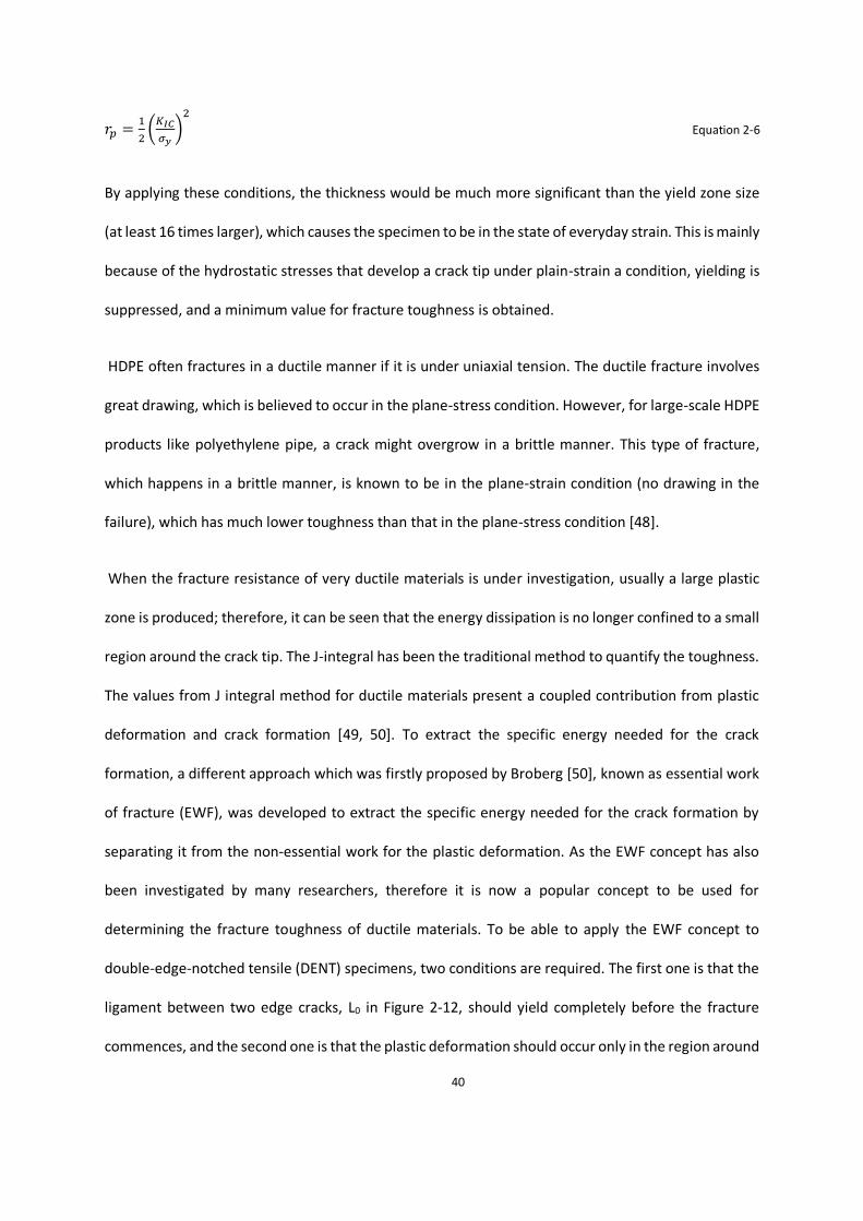
40

𝑟𝑝 =1

2(

𝐾𝐼𝐶

𝜎𝑦)

2

Equation 2-6

By applying these conditions, the thickness would be much more significant than the yield zone size

(at least 16 times larger), which causes the specimen to be in the state of everyday strain. This is mainly

because of the hydrostatic stresses that develop a crack tip under plain-strain a condition, yielding is

suppressed, and a minimum value for fracture toughness is obtained.

HDPE often fractures in a ductile manner if it is under uniaxial tension. The ductile fracture involves

great drawing, which is believed to occur in the plane-stress condition. However, for large-scale HDPE

products like polyethylene pipe, a crack might overgrow in a brittle manner. This type of fracture,

which happens in a brittle manner, is known to be in the plane-strain condition (no drawing in the

failure), which has much lower toughness than that in the plane-stress condition [48].

When the fracture resistance of very ductile materials is under investigation, usually a large plastic

zone is produced; therefore, it can be seen that the energy dissipation is no longer confined to a small

region around the crack tip. The J-integral has been the traditional method to quantify the toughness.

The values from J integral method for ductile materials present a coupled contribution from plastic

deformation and crack formation [49, 50]. To extract the specific energy needed for the crack

formation, a different approach which was firstly proposed by Broberg [50], known as essential work

of fracture (EWF), was developed to extract the specific energy needed for the crack formation by

separating it from the non-essential work for the plastic deformation. As the EWF concept has also

been investigated by many researchers, therefore it is now a popular concept to be used for

determining the fracture toughness of ductile materials. To be able to apply the EWF concept to

double-edge-notched tensile (DENT) specimens, two conditions are required. The first one is that the

ligament between two edge cracks, L0 in Figure 2-12, should yield completely before the fracture

commences, and the second one is that the plastic deformation should occur only in the region around

41

the ligament. When these conditions are followed, the energy absorbed during the test, after

normalised by the original ligament area, is known to be a linear function of the ligament length.

By using the concept above, work provided to fracture the specimen can mainly be divided into two

sections. The first section is the work for plastically deforming the region around the ligament, which

is expected to be proportional to the volume of the plastic deformation zone. If we assume that the

plastic deformation is completely developed before the crack growth commences, then it can be said

that the width of the plastic deformation zone, d in is then proportional to the initial ligament length,

L0, and the total work for plastic deformation, Wp, is proportional to L02×t0.

The second part is the essential work used for the formation of the fracture surface, We, which is

proportional to the CSA of the ligament L0×t0. By adding these two parts, it can be said that the total

work of fracture, Wf is;

𝑊𝑓 = 𝑊𝑒 + 𝑊𝑝 = 𝑤𝑒𝐿0𝑡0 + 𝛽𝑤𝑝𝐿20𝑡0 Equation 2-7

Where t0 is the initial specimen thickness, we the specific EWF, Wp the average plastic work density,

and β the shape factor for the plastic deformation zone. By measuring the total work of fracture for

specimens of different ligament lengths, and dividing Wf by the ligament CSA L0×t0, to the specific work

of fracture, wf can be expressed as;

𝑊𝑓 = 𝑤𝑒𝛽𝑤𝑝𝐿0 Equation 2-8

The specific EWF, we, can then be determined by extrapolating wf to zero ligament length.

42

Figure 2-12, Dent Specimen with FPZ zone shown

2.6.4 Fracture toughness range in high-density polyethylene

As polyethylene is one the most ductile materials, therefore its fracture at room temperature is usually

higher than 100%. As the fracture of polyethylene involves extensive necking, therefore it is

categorised to have ductile fracture; however, a pressurised polyethylene pipe can fail in a brittle

manner without any sign of necking. These kinds of failures are known as rapid crack propagation.

Different factors, such as high crack growth speed (sometimes exceeding the sound speed), low

ambient temperature, deformation constraint, etc. [50, 48, 51, 52]are known to prohibit neck

formation, resulting in brittle fracture behaviour. These are usually called plane-strain fracture, which

is opposite the plane-stress fracture that involves extensive necking. The toughness of polyethylene

in the two fracture modes is expected to be significantly different in the plane-stress fracture; the

toughness of polyethylene was reported to be above 30 kJ/m2. Some types of high-density

polyethylene (HDPE) were reported to show toughness around 35 kJ/m [53, 48]. The main reason it

must be considered that these values are measured in the plane-stress condition, with the

43

involvement of necking in the fracture process. These values are much higher than the steady-state

dynamic fracture toughness (Gd) of polyethylene pipe, estimated to be around 6 kJ/m2 [49].

2.6.5 Triaxiality

The stress triaxiality is usually represented as the dimensionless stress triaxiality ratio 𝜎∗. The

definition of stress triaxiality was shown by Hancock and Mackenzie [54].

𝜎∗ =𝐼1

3√3𝐽2 Equation 2-9

First stress invariant,𝐼1 = 𝑡𝑟𝜎, second stress invariant 𝐽2 =1

2𝜎𝑑𝑒𝑣: 𝜎𝑑𝑒𝑣 , 𝑤ℎ𝑒𝑟𝑒 𝜎 is the Cauchy stress

tensor, 𝜎𝑑𝑒𝑣 = 𝜎 −1

3𝑡𝑟(𝜎)𝐼 𝑖𝑠 𝑡ℎ𝑒 𝑑𝑒𝑣𝑖𝑎𝑡𝑜𝑟𝑖𝑐 𝑠𝑡𝑟𝑒𝑠𝑠 𝑡𝑒𝑛𝑠𝑜𝑟 and I is the second-order unit tensor.

Based on the above definition, it can be said that a uniaxial stress state in tension gives 𝜎∗=1/3

whereas a complete hydrostatic stress state in tension produces an infinity high-stress triaxiality ratio.

The triaxiality factor can also be defined as the ratio of hydrostatic pressure stress, or mean stress, σh,

to the Von-Mises equivalent stress, σeqv. The formula for the triaxiality factor is given below, where σ1,

σ2, and σ3 are the first, second and third principal stresses, respectively.

𝜎ℎ

𝜎𝑒𝑞𝑣=

1

3(𝜎1+𝜎2+𝜎3)

1

√2√(𝜎1−𝜎2)2+(𝜎2−𝜎3)2+(𝜎3−𝜎1)2

Equation 2-10

The influence of stress triaxiality on the failure mechanism of polymers has been investigated by

researchers recently. It has been found that an increase in stress triaxiality would accelerate void

growth, which is one main form of polymer failures, especially at higher thicknesses. It has also been

found that different triaxiality rate would not have an effect on the yield load but influences the

yielding of the failure directly. As yielding of a specimen (more yield means energy to break the

specimen) is an indication for the failure therefore, triaxiality would be an important factor in this

research [55] [56].

44

In chapter 5, the application of triaxiality in this study is demonstrated, and it is shown how triaxiality

could affect the failure behaviour of plastics.

Summary

In summary, in this section, different types of mechanical testing used for quantifying the quality of

butt fusion welding and HDPE are explained. Current methods of investigating the fracture toughness

of plastic materials, including their advantages and disadvantages, are also explained. The testing

geometry selected to be optimised and the factors such as energy to break which is a similar approach

as EWF concept, are selected and are fully described in the sections which they have been used.

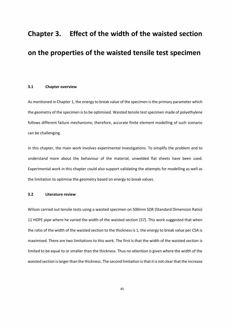
45

Chapter 3. Effect of the width of the waisted section

on the properties of the waisted tensile test specimen

Chapter overview

As mentioned in Chapter 1, the energy to break value of the specimen is the primary parameter which

the geometry of the specimen is to be optimised. Waisted tensile test specimen made of polyethylene

follows different failure mechanisms; therefore, accurate finite element modelling of such scenario

can be challenging.

In this chapter, the main work involves experimental investigations. To simplify the problem and to

understand more about the behaviour of the material, unwelded flat sheets have been used.

Experimental work in this chapter could also support validating the attempts for modelling as well as

the limitation to optimise the geometry based on energy to break values.

Literature review

Wilson carried out tensile tests using a waisted specimen on 500mm SDR (Standard Dimension Ratio)

11 HDPE pipe where he varied the width of the waisted section [57]. This work suggested that when

the ratio of the width of the waisted section to the thickness is 1, the energy to break value per CSA is

maximised. There are two limitations to this work. The first is that the width of the waisted section is

limited to be equal to or smaller than the thickness. Thus no attention is given where the width of the

waisted section is larger than the thickness. The second limitation is that it is not clear that the increase

46

in the energy to break per CSA is only from the extension in the middle of the specimen and not the

elongation in holes.

One of the methods which have been used widely to determine the fracture toughness of the

polymers is linear elastic fracture mechanics (LEFM), which uses the K IC and GIC parameters in the

brittle region of polymers [58, 59]. The brittle region of polymers is usually at a high strain rate or low-

temperature testing condition. When polymer behaviour is in the region of ductile behaviour, the

linear elastic stress intensity factor KI cannot be used to describe the stress condition in this type of

failure, and different methodology which is a non-linear elastic fracture mechanic methodology

(NLEFM) by using either CTOD or J integral [60, 61, 62].

When investigating the fracture behaviour of polymers in the ductile-to-brittle region is neither

completely brittle nor entirely ductile [63, 64, 64, 65]. Load-displacement data for polymers are always

non-linear, and consequently, LEFM presents difficulties when used within the transition region. While

using these techniques for polymers, operating in the ductile and the ductile-brittle transition region

present doubt about their toughness value. The abovementioned methods, regardless of covering the

linear and nonlinear behaviour of polymers are mainly based on a small plastic zone around the crack

tip. However, the values found from techniques such as J-integral presents coupled contribution from

plastic deformation and crack formation [66].

As a result of these complications to quantify the toughness of polymers, a different approach was

proposed by Broberg [50] known as essential work of fracture (EWF), which was developed to identify

the specific energy needed for the crack formation by separating it from the non-essential work for

the plastic deformation.

Different researchers investigated and applied this technique to quantify the toughness

characterisation of ductile materials. To apply the EWF concept correctly, there are some

47

requirements. The first requirement is to have the ligament between two edges crack and yield

completely before the fracture takes place. The other requirement is to have all the plastic

deformation to be around the ligament. When these procedures and requirements are met, the

energy used to deform the specimen, after getting normalised by the ligament area, will be a function

of the ligament length (Figure 3-1).

The specific EWF contains energy for mainly two deformations. The first one is the energy for necking

inside the fracture process zone (FPZ), which is the circle around the ligament or width of the waisted

section. The second one is the energy for generating a new fracture surface [52]. As mentioned

previously, some polymers especially high-density polyethylene, undergoes a high strain-hardening

behaviour in large deformation, which usually produces a stable neck development. The techniques

to measure the fracture toughness of polymers as mentioned above have mostly been tested on thin

sheets of polymer (maximum 6mm) [48] and have investigated transition of plane strain to plane

stress by adjusting the ligament length. The ability of the polymeric material to undergo a stable neck

development before it fails or fractures is essential for HDPE in applications such as pipeline or

pressure vessels that are used to distribute oil and gas. However, despite extensive research [67, 68,

69, 70] and its importance in industries, the mechanism involved in necking and its criteria requires

more investigations due to a lack of quantitative investigations.

48

Figure 3-1. Dent Specimen with FPZ zone shown [48]

The previous studies on necking behaviour or the fracture of polymers such as HDPE were mainly on

strain rate, temperature and initial imperfection size and less on geometry effect of the specimens.

Thus, the objective of this part of this chapter is to understand the geometry influence, especially the

width of the waisted section or ligament on different thicknesses (15 and 25mm) and aspect ratio

(width of the waisted section to thickness) of the specimen.

Problem definition and research methodology

The specimen which is under investigation in this chapter is waisted tensile test specimen used in ISO

13953, EN 12814-2, EN12814-7 and WIS 4-32-08 and is used to quantify the quality of butt fusion

welds. Regardless of the thickness of the pipe, many of these standards use similar geometries to

quantify the quality of the weld. The examination is usually by tensile testing and by examining the

fracture surface quality for acceptance of the weld quality. As mentioned in Chapter 1. , the work

carried out by Chipperfield [71] has shown that as well as fracture surface quantification, energy to

break the specimen per CSA could be a suitable indication to quantify the quality of the weld. The

visual assessment of butt fusion weld sample in WIS 4-32-08 is shown below.

49

In WIS4-32-08 different fracture surface modes is shown in Figure 3-2, and from the left, it has been

called Ductile, Mixed and brittle failure. When investigating the waisted specimen geometry

experimentally, it should be tested and cut from a welded pipe, but HDPE failure behaviour in normal

conditions performs a complex behaviour with different uncertainty and still with difficulties to predict

its failure behaviour. Having specimens from welded pipes adds two parameters into our problem

equation with no data on how they will affect the failure mode of the specimen:

◼ The first parameter is the curved geometry which will lead the specimen to be bending

perpendicular to the loading axis

◼ The other parameter has welded specimen, which will have a polymer with slightly different

material property in our waited area as well as some difference in thickness due to the weld around

the specimen.

Experimental setup

In order to focus on the effect of the width of the waisted section, unwelded flat sheet HDPE has been

used. The sheets had thicknesses of 15mm and 25mm. All the specimens in this work have been cut

and tested in the extrusion direction. The first sets of experiments are designed to fully understand

the effect of the width of the waisted section in thickness of 15mm. The thickness of 15mm has been

chosen to assure all the specimen fail in a complete ductile manner. As unwelded flat sheets are used

to only study the effect of the width of the waisted section, side plates have also been used to limit

the movement and extension of the specimen to be only around the waisted area (Figure 3-3).

50

Figure 3-2, from left ductile, brittle and mixed failure mode according to WIS 4-32-08

.

Figure 3-3, from left tensile testing with and without side plates

There are mainly four experiments carried out in this chapter. The first experiment is carried out on

15mm thickness with side plates, and the width of the waisted section varied from 3 to 35mm. Having

the width of the waisted section to be varied from 3 to 35mm will give an aspect ratio of 0.2 to 2.3 for

the width to thickness of the specimen.

The second experiment is carried out on 25mm thickness using side plates, and the width of the

waisted section is varied from 5 to 45mm, which produces an aspect ratio ranging from 0.2 to 1.8.

51

Experiments 3 and 4 are designed after the results from the first two experiments are investigated,

which will be described fully in the result and discussion section.

Table 3-1, Set of Experiments carried out to investigate the effect of the waisted section

Experiment

no

Specimens Thickness

(mm)

Width

(mm)

Side

plate

Welded Flat

1 11 15 3 to 35 Yes No Yes

2 10 25 5 to 45 Yes No Yes

3 6 15 12.5 to 22.5

No No Yes

4 6 25 15 to 27.5 No No Yes

Results and discussion

For each specimen, the force-deformation curve is recorded, which total energy to break of the

specimen per CSA calculated from force-deformation data. Before tensile testing, each specimen is

measured accurately to know the exact CSA. This CSA is the initial CSA before the test takes place,

and the CSA is not updated or calculated during deformation; therefore, the energy to break over the

CSA is based on a constant value for the CSA.

Figure 3-4 shows the total energy per CSA against the width of the waisted section for experiment 1.

As mentioned before, for these specimens, all the geometric parameters have been kept constant

(same value as stated in BS EN 12814-7 standard), which means 20mm for loading hole diameter,

90mm for the distance between loading holes, 60mm for width of the specimen, 5mm for radius of

the waisted section and 170mm for total length of the specimen. It is evident that, by increasing the

width of the waisted section, the energy to break per CSA increases, except from 20mm to 25mm.

From the overall result by comparing total energy to break against the width of the waisted section, it

52

could be concluded that more investigation regarding this type of comparison and measurement must

take place.

Figure 3-4, Graph shows the total energy to break value per CSA against the width of the waisted section for 15mm sheet

thickness with side plates (Experiment 1)

Since the necking of the specimen is in the area of interest, the first step for in-depth investigation is

to quantify the amount of total energy to break that has been consumed for the necking of the

specimen. This is shown in Figure 3-5, where the force-displacement curve is divided into four

different regions:

• Region one is from the beginning of the test till the beginning of necking.

• Region two is from the beginning of the necking to the start of the cold drawing, and this can

also be called the neck formation region.

• Region three is mainly a cold drawing region.

• Region four is the tearing section.

53

The method used to distinguish these regions is that the differentiation of the data, which is energy

per CSA, is taken, and on the step or the moment, the differentiation value reached zero (means a

complete change in gradient of the curve) is assumed to be the moment where the different region in

these fractures has started.

As shown in Figure 3-6, Regions 1, 2 and 3 indicate that when the width of the waisted section

increases, the energy to break value per CSA also increases accordingly. Region three is the cold

drawing region with the highest energy per CSA.

Figure 3-5, Graph shows the force-displacement curve for specimen no PEW02, divided into four regions

54

Figure 3-6, Energy to break values of different regions against the width of the waisted section for the first

experiment

Experiment 2 is also designed to investigate the effect of the width of the waisted section. The

specimen numbers with the dimension can be seen in Appendix A. By investigating the force-

displacement curves Figure 3-7 it can be seen that region three is non-existent for this experiment.

When the width of the waisted section just reached 25mm, Region 3 seems to be appearing again,

which could be mainly due to two reasons. First is mainly because it is becoming closer to the thickness

value (it would have a more uniform cross-section and reduces the triaxiality factor), the second

reason is that the pin diameter is 20mm, and as the width is becoming larger than the loading hole

55

diameter, it causes more deformation throughout the specimen; therefore the specimen consumes

more energy to break.

Figure 3-7, Load-displacement for 20mm and 40mm width of the waisted section

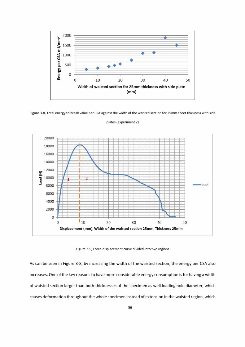
56

Figure 3-8, Total energy to break value per CSA against the width of the waisted section for 25mm sheet thickness with side

plates (experiment 2)

Figure 3-9, Force-displacement curve divided into two regions

As can be seen in Figure 3-8, by increasing the width of the waisted section, the energy per CSA also

increases. One of the key reasons to have more considerable energy consumption is for having a width

of waisted section larger than both thicknesses of the specimen as well loading hole diameter, which

causes deformation throughout the whole specimen instead of extension in the waisted region, which

57

is our area of interest. To eliminate other factors (energy consumed to elongate the hole), the force-

displacement graph is divided into two sections (Figure 3-9), and energy per CSA against the width of

the specimen is displayed Figure 3-10. It can be concluded from both regions that increase in the width

of the waisted section gives rise to an increase in the energy content of region one as well as the

energy in after the yield section. This experiment could not be conclusive as most of the failures are

not ductile, and if they are ductile, they failed due to void growth. The few specimens that failed in a

ductile manner had substantial deformation in loading pin diameters which shows a significant error

in the test result. This is also including the energy consumed for the deformation of the areas which

are not in our area of interest (the waisted area).

Side plates are used to limit the deformation on the waisted area and eliminate deformation over the

specimen as well as understand its effect on the failure behaviour. However, in standards used to

quantify the quality of welds, specimens that are cut from welded pipes are tested without side plates.

It is notable that using side plates can have some disadvantages not only from time and cost, which

would require side plates for every pipe size but also as it fully limits the deformation of the specimen

to the waisted region, it does not allow a uniform stress distribution in the waisted section. Due to the

factors mentioned above, the next few experiments are designed without having side plates in the

test.

58

Figure 3-10, Total energy to break value per CSA against the width of the waisted section for 25mm sheet thickness with

side plates (experiment 2)

Experiment 3 is on 15 mm HDPE sheet but without using side plates. The results from this experiment

have been compared with the first experiment against energy consumption per CSA for each of the

four mentioned regions. As can be seen in Figure 3-11, energy per cross-section area increased with

an increase in width of the waisted section, which shows a similar trend for both experiments, which

59

are carried out with or without side plates. As described briefly earlier, the energy consumed in Region

one is used to take the specimen up to the yield point. As the width of the waisted section increases,

regardless of any other parameter, it would increase the energy consumed to yield the waisted region.

In the case of specimens without side plates, there has been higher energy used compared to the

condition with the side plate on larger width of the waisted section. This is due to the ability of larger

width, which has caused more deformation through the specimen compared to the condition with the

side plate; the deformation is limited in the waisted area. As the distance between the centre of the

specimen (waisted area) to the loading point is higher on the cases without side plates, more material

(plastics) is used to transfer the loads to the waisted area. This transformation of the load, which is a

larger area on specimens with no side plates would use energy to elongate and transfer the

deformation, which would affect the energy consumed and explains why there is more consumed on

the cases with no side plates. As the specimen with 25mm width was not following the trend, it was

repeated, and therefore, two sets of data points are available 25mm width with side plates.

Figure 3-11, Energy per CSA against the width of the waisted section on 15mm thick specimen with and without side plates

for Region 1

60

Energy used in Region 2 is an indication of energy used to bring the specimen from the necking or

yield point to the start of cold drawing. The energy consumed in this part does not provide any

discriminative information for experiments in both cases with or without side plates (Figure 3-12).


for Region 2

The comparison for Region 3 cold drawing and the main indication of ductility in a specimen provides

useful discriminative information. The average total energy used for specimens without side plates is

higher than the set of experiments using side plates. This is due to limiting the deformation in the

surface area of the specimen except for the waisted area while using the side plates, therefore

transferring all the strain rate directly to the waisted area. When the specimen is tested without side

plates, there are deformations throughout the whole specimen. Also, the strain rates applied from

loading holes are much lower in the middle of the specimen. This makes the tensile testing without

side plates more reliable.

The other finding from this analysis is that in both cases (with and without side plates) when the width

of the waisted section is equal to the thickness (both 15mm) the energy to break per CSA for Region

61

3 is maximised. One of the reasons is having a square CSA and therefore, more normal and axial

stresses (Figure 3-13).


for Region 3

Region 4 did not provide useful information, as it is an indication of tearing, and it is the step after the

cold drawing (Figure 3-14). To check and understand the effect of side plates on tensile tests, two

specimens, one from each set of experiment is selected. Load-displacement data is shown in Figure

3-15. The geometry factor for both specimens is the same, and the width of the waisted section for

the specimen is set to be 15mm. The behaviour of both specimens is similar throughout most of the

test except in the necking section. The necking points are the same as well as the stress for necking

the specimen. This comparison suggests that using side plates produces limitation to the test and

decreases the ductility in the specimen.

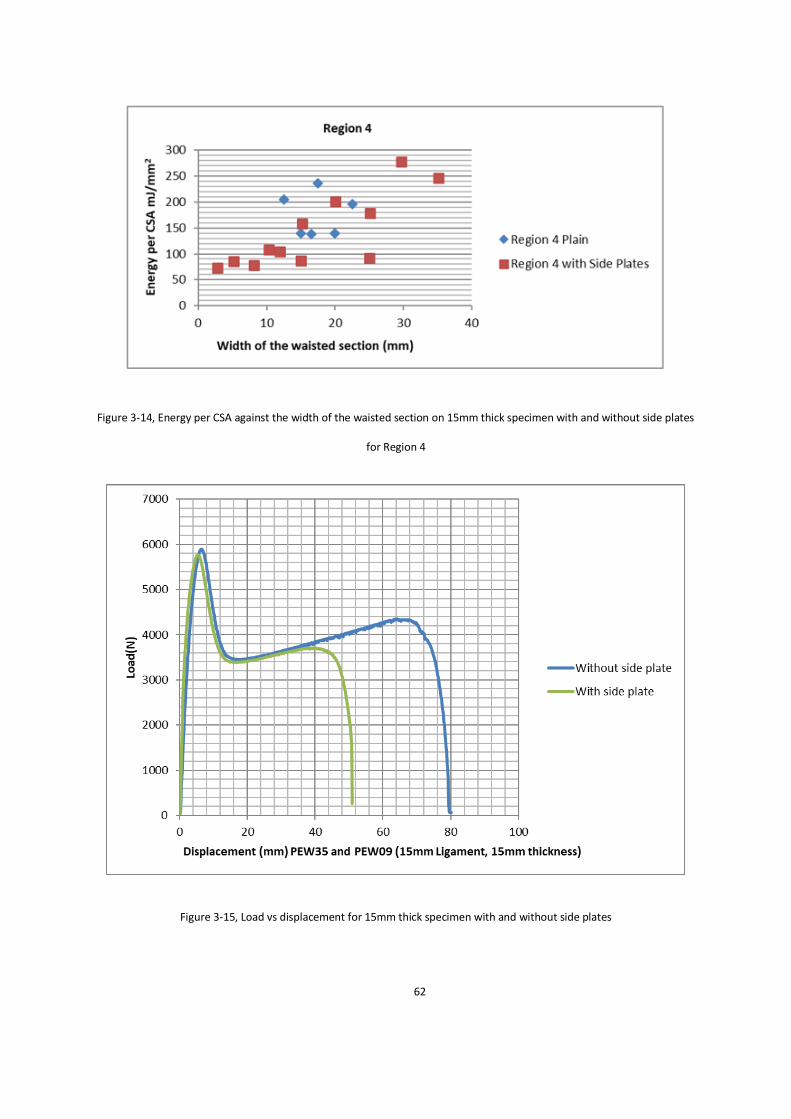
62


for Region 4

Figure 3-15, Load vs displacement for 15mm thick specimen with and without side plates

63

After understanding the effect of side plates and the width of the waisted section, the next experiment

is carried out without side plates using specimens with 25mm thickness. The width of the waisted

section for this set of experiment is varied from 15mm to 27.5 mm (Figure 3-16).

Figure 3-16, Load-Displacement curve for 25mm thickness with 15mm to 27.5mm in width of the waisted section (in order,

from the smallest to largest graph, where 15mm is the smallest and 27.5 is the largest)

In this set of experiment, most of the specimens failed in a manner that no cold drawing occurred in

most of the specimens. The only specimen where Region 3 (cold drawing region) appeared is the

specimen with 27.5mm width of the waisted section. Since the thickness of the specimen is 25mm,

large elongation in loading pinholes appeared during the tensile test. The fracture surface of a

specimen from this experiment is the right specimen in Figure 5-25 which has a width of the waisted

section of 27.5mm.

64

Summary

Experimental investigations carried out in this chapter resulted in useful information as to how the

parent material fails using waisted specimen geometry, specifically 25mm thickness specimens. This

shows the gap in the knowledge and confirms the need to solve this substantial industrial problem in

assessing the quality of butt fusion welds.

Experiments were carried out on a non-welded, flat sheet of specimens without any particle (Carbon

Black). Despite these simplifications, there was yet no possibility of ductile failure in specimens with

25mm thickness as they failed from void growth. This indicates the lack of appropriate procedure and

an acceptable standard to quantify the quality of welds at this thickness or above.

The other conclusion is the effect of the side plates which reduces the ductility of the specimen. Also,

the effect of the width of the waisted section has shown to be at maximum energy to break when it

has an aspect ratio of one to the thickness. This finding is further investigated using FEA analysis to

confirm this phenomenon.

It can also be hypothesised that, as the thickness of the material exceeds a specific value, the fracture

behaviour of the specimen completely changes. This means, if any optimisation is carried out on these

specimens, the first step is expected to involve making sure that all specimens fail in the same manner

(ideally ductile with elongations) so that the effect of each parameter can be observed and recorded

accordingly. This investigation is covered in the next chapter.

65

Chapter 4. Effect of different parameters of waisted

tensile test specimen using DOE optimisation

Chapter Overview

This chapter investigates the geometry effect of the waisted tensile test specimen (Figure 4-1) on the

energy to break value using CCD (Central Composite Design) optimisation technique. This technique

which is one of the design of experiments (DOE) optimisation methods combined with response

surface methodology, is explained in the literature section of this chapter and used in this chapter.

CCD applied to understand the effect of geometry factors such as; width of the waisted section, the

radius of the waisted section, loading hole diameter, distance between the loading holes and width of

the specimen independently and dependently against different responses. Responses used in this

study are;

• Total Energy to Break value of the specimen

• Energy consumed in the cold drawing stage

• Elongation of the loading hole

Justifications for selecting the named factors and responses are explained in depth in this chapter.

Experimental methodology, as well as the findings in the forms of graphs and equations, are presented

in this chapter. At the end of this chapter new optimised geometry with different dimensions for the

thickness of 15mm is proposed.

66

Literature review

As mentioned in the overview section, to optimise the specimen geometry, the following parameters

are investigated; width of the waisted section, the radius of the waisted section, loading holes, the

distance between loading hole diameter and width of the specimen.

Figure 4-1, Waisted tensile test specimen (EN 12814-7) (dimensions in mm)

To investigate the effect of these parameters, a set of experiments had to be designed. Previously,

experiments were carried out by changing one-factor at-a-time; however, this type of approach is

expensive and time-consuming due to the many tests required. Another disadvantage of changing the

factors one-at-a-time is that the factor interactions cannot be identified. Therefore, techniques that

can provide better solutions with a lower number of experiments, such as the design of experiments

(DOE), Artificial Neural Network (ANN) etc., are preferable [72, 73].

67

The design of experiments is a statistical technique that is used for multi factors system optimisation.

As mentioned earlier design of experiments will be used to carry out a lower number of experiments

rather than experimenting with every combination. Based on the number of factors and the number

of experiments we can carry out, there are different optimisation types within DOE that could be

selected to design the experiments. Central Composite Design (CCD) and Box-Behnken Design (BBD)

are two common types where more than three factors are being optimised [74].

A review study carried out by Benyonis and Olabi [75] on different techniques of optimisation for

mechanical properties of different welding techniques suggested that a response surface

methodology (RSM) performs better than other techniques, especially when a large number of tests

cannot be carried out. The main benefit of applying the RSM technique is its ability to indicate each

factor's effect on different responses from coefficients in the regression model. This advantage can be

used in identifying the insignificant factors main effect, insignificant interactions and insignificant

quadratic terms in the model, which means that those factors can be removed, which helps in reducing

the complexity of the model. The most popular methods within the RSM techniques are CCD and BBD.

RSM technique generally is widely used in mathematics, and statistics is a known tool for modelling,

which eases the process of optimisation when the effect of factors are interactions are required. This

will also allow having a great estimate on a condition where the actual test has not taken place [76].

To be able to apply the RSM technique to optimisation, the factorial design of the experiment must

include centre points in the experimental space plus edge centre points or face centre points. These

multilevel experimental points allow fitting the responses to quadratic or cubic equations. CCD is one

the best methods which would be suitable for RSM due to being a two-level factorial design with

additional points to be outside the range of the factors, points between the axes (star points) and

repeated points at the centre. Depends on the application where CCD is used, the start points at the

face may extend, but in most cases, it is located on the plane with other coordinates. Below is the

experimental space for a three-factor CCD [77, 78].

68

Figure 4-2, Central Composite Design (CCD) experimental space [77]

If optimisation is carried using any of DOE techniques, it can still be processed without RSM, but only

the result of the carried out tests from the experiments could be seen, and the results for the

interaction of factors would be unknown.

In summary, CCD, a method of DOE, is used just to design the experiment and RSM is used to analyse

the data and the output of the experiment.

For this study, the CCD technique is applied to have the minimum number of runs and get the full

information regarding the effect of each factor and factor interactions effect.

Experiment

4.3.1 The material, sample preparation, and testing

A commercial extruded HDPE sheet of 15mm supplied by Amari Plastics (UK) was used for this study.

The tensile yield strength of the material is 22MPa with a modulus of elasticity of 900MPa. The

specimens were prepared and machined using an Isel CNC machine and were conditioned for a

minimum of 24 hours before performing the tensile test. The tensile tests were carried out according

to EN12814-7 condition (not the geometry dimensions) with a speed rate of 5mm/min. The tensile

69

test machine used to carry out this experiment is a Hounsfield servo-electric tensile machine with a

maximum tensile capacity of 50kN.

4.3.2 Design of experiment and characterisation

Design expert software (stat-ease) is used to design a 5-factorial CCD. As the objective of this study is

to investigate the effect of each parameter in the geometry, the effect of specimen thickness is not

investigated in this study because increasing thickness changes the failure mode from ductile to

brittle, making the DOE invalid as it will not allow the specimen to fail in the same manner.

The initial test matrix consisted of 50 test specimens, and the limits of each parameter are based on

the specimen dimensions given in the current standard. To set the limits for the width of the waisted

section, 25 mm is set for the high limit, and 15 mm is set for the low limit. The high limit is the value

given in BS EN 12814-7, and the low limit is selected as 15 as previous work carried by Wilson et al. [7]

suggests that a ratio between the specimen thickness and the width of the waisted section of one to

one produces the highest energy to break per unit area.

The low limit of the radius of the waisted section, 5mm, is therefore defined in BS EN 12814-7 since

an increase in radius will reduce the stress concentration. The high limit of this parameter is selected

as 10mm. The other three parameters' effect is not apparent, so the standard dimensions given in BS

EN are set to be at the middle of the design. The table below shows the values and limits of the design.

70

Table 4-1, Variables used in the central composite design

Parameters Levels used

Low (-1) Middle (0) High (+1)

The width of the waisted section, mm

15 20 25

The radius of the waisted section, mm

5 7.5 10

Loading hole diameter, mm 15 20 25

The distance between the loading hole, mm

80 90 100

The width of the specimen, mm 60 70 80

The different regions of a typical force-displacement graph for HDPE are shown in (Figure 4-3). Like

any other optimisation design, the optimum solution is based on having an optimum response. The

primary response and characterization used in this study is the total energy to break value per unit

cross-sectioned area at the waisted section, i.e., the area under the force-displacement curve divided

by the CSA of the waisted section. Indicating Region 3 is mainly an indication of energy being used for

the cold drawing region. The cold drawing or necking region starts when the neck is fully developed

and ends just before tearing (completed shear yielding) of the specimen.

The other response that is investigated is the Region 3 energy per unit CSA. The final response is the

deformation in the loading holes. When the energy to break the specimen is calculated from the area

under the curve of force vs displacement of the loading pins, any deformation of the loading pin holes

introduces energy since the measured energy will consist of the energy to break the specimen as well

as the energy to elongate the loading pin holes.

71

Figure 4-3, Example of a typical Force-Deformation graph

Results and Discussions

To understand the effect of each parameter on a particular response, a model is fitted for each

response. All three responses are analysed statistically using analysis of variance (ANOVA) in order to

determine the effect of the five specimen geometry parameters (width of the waisted section, the

radius of the waisted section, the diameter of loading holes, the distance between loading holes and

width of the specimen). Complete tensile tested specimens for this study are shown in Figure 4-4.

72

Figure 4-4, Tensile tested specimens for the DOE experiment

4.4.1 Optimisation of Total Energy Factor

Table 8-5 in the Appendix shows the results of the ANOVA analysis for the total energy to break value.

The ANOVA table shows the sum of the squares (SS) and means square (MS) of each parameter where

the P-value and F-ratio are defined as the ratio of respective mean square effect and the mean square

error. To consider a constant, any confidence level can be used considering how vital the parameter

is to the design, but for a 95% confidence level, an effect is called significant when the P-value is less

than 0.05. By investigating the P-values in Table 8-5, the whole model, which consists of 18 terms, is

a significant model with P-value of <0.0001. The three parameters that show the most significant are

the width of the waisted section, the radius of the waisted section and distance between the loading

holes with P-values of 0.0009, 0.0002 and 0.0043 respectively. The diameter of loading holes and

width of the specimen which in order had P-values of 0.3466 and 0.3495 despite having a lower

73

significance but as they have about 65% confidence level, it is decided to consider them for analysis.

As shown in Table 8-5 interaction effects of AE, BD, C2 and A2 also are also statistically significant.

To be able to model this optimisation for one response, an equation is produced by the stat ease

software, which works based on principle curve fitting similar to finding an equation of a line used in

excel. The line is the equation of the experiments carried out, and it must be as close to experimental

values as possible. This line could be 1st order or curved of the 2nd order or 3rd order with some

constants and coefficients as listed in equation 4-1 as an example. The target is to find this equation

so we can discover the values of areas (factor combinations) where we did not carry out experiments,

but they are interesting areas. To have a more accurate curve fitting technique or equation, the

coefficient of combination of factors are checked, and they are used as constants in the equation,

which represents how significant their effects are on the response. As mentioned, if these coefficients

are large, then they will be used in the equation, and if they are small, it means the effect of the

interaction for these factors are small, and they should be removed. As equations 4-1, 4-2, 4-3 are a

multiple dimension equation, graphically, it is not possible to show the curve fitting image.

Before finalising the ANOVA table, many model types with a different number of terms are studied,

but after investigating the significance of the terms and comparing the predictions with the actual

values, this model, which is a modified quadratic model, is chosen. The total energy to break (per unit

CSA) value can be calculated using the equation below.

𝑇𝑜𝑡𝑎𝑙 𝐸𝑛𝑒𝑟𝑔𝑦 = 1678.75 + 41.80𝐴 + 402.33𝐵 + 45.34𝐶 + 151.01𝐷 + 5.04𝐸 −

108.98𝐴𝐸 + 102.21𝐵𝐷 + 62.99𝐶𝐷 − 69.47 𝐴2 − 235.98 𝐶2 + 44.14 𝐷2 −

51.05 𝐸2 Equation 4-1

In Equations 4-1, 4-2 and 4-3, A stands for width of waisted section, B for radius of the waisted section,

C for diameter of loading hole, D for distance between loading holes and E for width of the specimen.

74

Equation 4-1 includes a large number of terms. Some terms with low coefficient could be removed

from the equation, but then it would reduce the model's accuracy. A graph to analyse the model's

adequacy by showing the relationship between the actual and predicted values of total energy to

break is shown in Figure 4-5. Figure 4-5 is produced to show the quality of the fitting process. The

points (each point is a combination of factors) near the diagonal line indicate a better model as they

have a value closer to the actual value, therefore if a combination is selected with conditions close to

these points, there would be more confident in the accuracy of the results.

Figure 4-5, Total energy to break values per unit CSA

This figure indicates that the overall developed model is adequate. This is because residuals of many

terms in predictions of each response are minimal since the residuals tend to be close to the diagonal

line. The main effects and surface plots are generated to represent the results of the polynomial model

analysis. The main effects of each parameter on the total energy to break value response is presented

in Figure 4-6. This figure is a direct output of the software.

75

Figure 4-6, Main effect plot for total energy to break per unit CSA value for specific terms

There are two facts to be considered when investigating graphs in Figure 4-6. The first fact is

understanding the graph indicates the main effects, which show the deviation of the average between

high and low levels for each parameter. The second important fact is that the effect of each parameter

on a specific graph is only valid for the stated value of the other factor; these factors interact with

each other, and when investigating one of the parameters, the other four parameters are kept

constant. If these constants changes, these factors would have a different effect on the total energy

to break per CSA value.

From Figure 4-6, it can be seen that increasing the width of the specimen, the distance between the

loading holes and the radius of the waisted section increases the total energy to break values. There

76

are several reasons for this increase. Increasing the distance between the loading holes or width of

the specimen increases the volume of material between the loading pin holes, which causes more

loads to be allowed due to the larger amount of material, which leads to higher total energy to break

values. The increase in distance between loading holes and the radius of the waisted section also

causes the stress distribution to be more uniform in the waisted section, which will help the specimen

to have a longer necking stage.

Increasing the radius of the waisted section will also reduce the stress concentration in the waisted

section. Despite calculating the energy to break values based on CSA to eliminate the effect of the

volume of material in the waisted section, but the effects still can easily be seen due to the behaviour

and characteristics of the material. This can also be explained with the mechanism polymers handle

the load, which to transfer load on each particle, the material could undergo elastic and hyper-elastic

deformation before transforming the load.

The increase in diameter of the loading hole leads to a decrease in total energy to break value in the

specimen. This could be because of the larger contact surface of the loading pin to the specimen hole’s

which causes a more significant stress distribution around the pin and the specimen. The optimum

value for the width of the waisted section is around 17mm, which then reduces when the width of the

waisted is increased.

4.4.2 Optimisation of Region 3 Energy Factor

Table 8-6 shows the results of the ANOVA analysis for the Region 3 of the force-displacement curve

as indicated in Figure 4-3. From the P-value in Table 8-6, it can be seen that the width of the waisted

section, the radius of the waisted section and the distance between the loading holes and their

interactions are statistically significant. The diameter of the loading hole and width of the specimen

have large P-values, but they have been included in the analyses because they are two of the main

77

parameters in the analysis and some of their interactions with other parameters are also statistically

significant. After considering the significance of the parameters and analysing the predicted vs actual

values, the model in coded units is found. The total Region 3 energy to break value based on coded

levels can be calculated using Equation 4-2.

𝑅𝑒𝑔𝑖𝑜𝑛 3 𝐸𝑛𝑒𝑟𝑔𝑦 = +1166.83 − 42.73𝐴 + 390.03𝐵 + 76.69𝐶 + 144.69𝐷 + 32.12𝐸 −

88.11𝐴𝐸 + 123.18𝐵𝐷 − 49.12𝐴2 − 257.90𝐶2 + 41.13𝐷2 − 73.52𝐸2

Equation 4-2

From the coefficients of The total Region 3 energy to break value based on coded levels can be

calculated using Equation 4-2, the distance between the loading holes has the most significant effects

on the Region 3 energy, followed by the radius of the waisted section and width of the waisted section.

Figure 4-7, shows the plot of actual versus predicted values for Region 3 energy per unit area. It shows

the adequacy of the model is certain small points and there few points with low Region 3 energy and

very high Region 3 energy which have large adequacy.

Figure 4-7, Region 3 energy to break values per unit CSA

78

The main effects of each parameter on the Region 3 energy are shown in Figure 4-8, which shows the

increase in the radius of waisted section and distance between the loading holes increases the Region

3 energy. Figure 4-8 also shows that the width of the waisted section increases the Region 3 energy

when it is in the range of 15 to 17mm. Other two parameters, which are the width of the specimen

and diameter of the loading holes, do not seem to have much effect on Region 3 energy.

Figure 4-8, Main effect plot for Region 3 energy

When performing the tensile test on the standard geometry of waisted tensile test geometry, the

deformation applied to the specimen does not always fully deforms the waisted section but deforms

the loading hole pin and the materials between the loading holes as well as the waisted section. As

the weld line is in the waisted section and energy used to deformed the specimen is the indication of

the quality of the weld; therefore, it is important to have most of the deformation in the waisted

79

section. One way to make sure the deformation has taken place in the waisted section is to check the

elongation in the loading pin diameter. For example, if the loading hole diameter is 20mm before

performing the tensile test, and the loading hole diameter after the specimen's failure is 20.2 mm, the

loading hole has gone through more considerable deformation. After recovering the elastic

deformations, the permanent plastic deformation in the hole is about 0.2mm. The permanent

elongation in the loading pinhole has been taken as one of the minimise responses for this analysis.

4.4.3 Optimisation for Loading Pin Holes Factor

The ANOVA analysis results for elongation in the loading pinhole is shown in Table 8-7.

As can be seen from P-value in Table 8-7, the width of the waisted section and the width of the

specimen are statically significant. The distance between the loading hole and the radius of the listed

section does not seem to have any effect; therefore, they have not been included in the ANOVA table.

The obtained model is coded units are presented in Equation 4-3 as;

𝐷𝑒𝑓𝑜𝑟𝑚𝑎𝑡𝑖𝑜𝑛 𝑎𝑡 𝑙𝑜𝑎𝑑𝑖𝑛𝑔 𝑝𝑖𝑛 ℎ𝑜𝑙𝑒 (𝑚𝑚) = +0.38 + 0.30𝐴 − 4.709𝐸 − 003𝐵 − 0.063𝐶 −

0.051𝐷 − 0.098𝐸 Equation 4-3

From the coefficients in Equation 4-3, it can be seen that two parameters are missing due to their low

effect and the diameter of loading holes have a slightly lower coefficient compared to the width of the

waisted section and width of the specimen. Figure 4-9 shows the plot of actual versus predicted values

for the elongation in the loading pinhole. As a linear model is fitted for this analysis, the difference

between the predicted and actual values are not perfectly aligned due to the simple modelling of this

response. The line is fitted as an estimate to have an equation to predict the actual values using the

stat ease software. This is similar to excel when a line (with equation) is fitted to a graph, and it can

become more accurate by increasing the order of the equation.

80

Figure 4-9, Elongation in the loading pinhole

The main effect of each parameter on the elongation in the loading pinhole is shown in Figure 4-10.

From Figure 4-10, the increase in width of the waisted section leads to an increase in deformation at

the loading pinhole. This is mainly due to increasing the cross-sectional area of the waisted section,

which is also the area of interest to perform the necking. By increasing the cross-sectional area, the

force to neck that region is increased, which would require the whole specimen to undergo a more

considerable amount of force that leads to elongation in the loading pinhole. Increasing the diameter

of the loading hole leads to a decrease in deformation at the loading pinhole. This could mainly be due

to the increase in the top surface area of the loading pin, which helps to transfer the load required to

neck the material to more regions of the specimen without elongating the hole. The increase in the

total width of the specimen also leads to a decrease in deformation at a loading pinhole. This could

be due to the increase in the material on the sides of the loading pin hole, which reduces deformation

on regions around the loading hole by holding the materials together.

81

Figure 4-10, Main effect plot for elongation in the loading pinhole.

Maximisation and minimisation of the responses

For this optimisation study, three energy responses are required to get maximised simultaneously,

and one response which is the deformation in the loading pinhole is required to get minimised. One

of the methods to solve multiple response optimisation problems is to use the desirability function

which is a useful approach to cut the dimensionality of a simultaneous optimisation problem to just

one. In this technique, each response equation is first transformed to an individual desirability

function (d) that varies over the range 0 ≤ d ≤1. Based on the need of the response there are, three

forms of a desirability function can be set to which are [79] :

• Larger better (LB) – for an object function of the response to be maximum;

82

• Smaller better (SB) – for an object function of the response to be minimized;

• and nominal better (NB) – for an object function of the response to attaining a specific goal.

In this study, three responses desirability function is the larger better (LB), and one response which is

the elongation in the loading hole is the smaller better (SB). The desirability function LB can be written

in an overall form shown in;

𝑑 = {

0 𝑦 < 𝐿

(𝑌−𝐿

𝑇−𝐿)𝑟 𝐿 ≤ 𝑦 ≤ 𝑇

1 𝑦 > 𝑇

Equation 4-4

Where y can be called as the response, L would be the lower limit of the response, T is the target of

the response, and r is the weight factor. The desirability function of the smaller better (SB) where U

would be the upper limit and the function can also be written as in the form of [79];

𝑑 = {

0 𝑦 > 𝑈

(𝑌−𝐿

𝑇−𝐿)𝑟 𝑈 ≥ 𝑦 ≥ 𝑇

1 𝑦 < 𝑇

Equation 4-5

In this study, the desirability (d) for each response is a unity that makes the composite desirability (D)

also unity. The composite desirability function (D) used in this study can be calculated as Equation 4-

6.

𝐷 = √𝑑1(𝑇𝑜𝑡𝑎𝑙 𝐸𝑛𝑒𝑟𝑔𝑦(𝑋)) × 𝑑2(𝑅𝑒𝑔𝑖𝑜𝑛 3 𝐸𝑛𝑒𝑟𝑔𝑦(𝑋)) × 𝑑3(𝐸𝑙𝑜𝑛𝑔𝑎𝑡𝑖𝑜𝑛 𝑖𝑛 𝑡ℎ𝑒 𝑝𝑖𝑛(𝑋))3

Equation 4-6

In the equation above, as mentioned before, D is the composite desirability function, X is the vector

of the designed variables (coded values), d1 is the individual desirability function corresponding to the

first response (i.e., total energy), d2 is the individual desirability function corresponding to the second

response (i.e., energy in Region 3) and d3 is the individual desirability function corresponding to the

83

third response. The desirability of all response and composite desirability have all been calculated

using STATE EASE software with the weight factor of r = 0.5. The result of the total desirability function

analysis is given in Figure 4-11. From Figure 4-11, it can also be seen that the desirability changes by

varying the value of the parameters. The least desired are shown by gree, and most desired are shown

by the orange, the colouring in between is the transition.

Figure 4-11, Desirability and parameters

The optimum solution suggested by the model had a combined desirability of 0.87 and individual

desirability of 0.822 for total energy, 0.825 for Region 3 energy and 1 for loading pinhole response.

The optimum solution, which considers all the responses, suggested 16mm in width of the waisted

section, 10mm for the radius of the waisted section, 20.8mm for the diameter of loading holes,

100mm for the distance between the loading holes and 68mm for the width of the waisted section.

To select the optimum geometry, these values have been rounded for ease of machining and have

been tested against BS-EN 12814-7 standard geometry, and the results can be seen in the figure

below.

84

Table 4-2, Optimisation results for predicted vs actual values

Parameters 12814-7 Geometry Improved Geometry

The width of Waisted Section (mm)

25 15

The radius of Waisted Section (mm)

5 10

The diameter of Loading Hole (mm)

20 20

Distance Between Loading Hole (mm)

90 100

Width of Specimen (mm) 60 70

Predicted/Actual Total Energy (mJ/mm2)

1250/1252 2330/2145

Predicted/Actual Region 3 Energy (mJ/mm2)

688/666 1906/1800

Predicted/Actual Elongation in Pin Hole (mJ/mm2)

0.67/0.6 0/0

In Table 4-2, parameter values for standard and improved geometries are shown. In addition to

parameters dimensions, predicted versus the actual values for three responses have been shown in

Table 4-2. The primary response, which is the total energy, has been improved from 1250 mJ/mm2 to

2140mJ/mm2, which is around 70% improvement. The Region 3 response, which is the cold drawing

region, had around 170% improve which shows a significant improvement. The elongation in the pin

has been reduced to 0, which is ideal and could not be improved in a better way.

Conclusion

The result of the ANOVA for total energy response and Region 3 response analysis shows that the

radius of the waisted section and distance between the loading holes were two of the most influenced

parameters which had the lowest P value. Despite some parameters such as the width of the waisted

85

section and width of the specimen, had larger P values in the first two responses (total energy and

Region 3), but these two parameters were two of the most influential in the elongation in the loading

pin response. The increase of parameters such as the width of the specimen, the distance between

loading holes and the radius of the waisted section has led to improving the total energy and Region

3 energy responses. Based on desirability function, the best combination for waisted geometry on

total energy, Region 3, and elongation in the pin response is 15mm for the width of the waisted

section, 70mm for the width of the specimen, 10mm for the radius of the waisted section, 20mm for

the diameter of the loading holes, and 100mm for the distance between the loading holes. Finally, all

the responses have been improved significantly with 70% of total energy, 170% for Region 3 energy

and zero elongation in loading pinholes and this trend can be used for larger thickness specimen.

86

Chapter 5. Modelling of necking in HDPE specimen

and effect of triaxiality factor

Chapter overview

This chapter investigates the effect of geometry parameters on the deformation of the waisted tensile

test specimen made of HDPE and the triaxiality in the middle section. The mechanical behaviour under

various stress triaxialities induced by different specimen thickness, notch radius, and width of the

cross-section of the specimen is investigated. The capacities of a constitutive model based on macro

deformation of polymers to model this material are also studied.

Literature Review

Plastic dilation and energy to break the specimen are the critical response parameters to evaluate the

ductility of the specimen and the flow potential of the constitutive model. It is found that plastic

dilatation and energy to break the specimen are highly sensitive to stress triaxiality [80].

The two key elements which perform an essential role in obtaining different failure modes are

different thicknesses of the pipes as well as the radius of the notch at the welded area of the specimen.

These are the two main reasons which can cause more production of the tension-dominated triaxial

stress state.

The geometry shown in Figure 4-1 is known to introduce transverse components to the stress tensor,

which produces a large triaxial stress state. The larger the thickness and smaller the radius of the

waisted section, the higher the stress triaxiality would be.

87

In a previous study [81] on a bar specimen made of HDPE, where the tension and compression are

equal, the plastic dilation in a uniaxial stress state is minor, whereas micro holes started to grow in

the centre of the HDPE specimens subjected to biaxial tension. This study shows that higher stress

triaxialities may trigger a damage mechanism that leads to micro ductile failure.

To investigate the triaxial stress state as well as experimental trials, modelling of HDPE with the

suitable material’s behaviour must be carried out. The problem in modelling polymers such as high-

density Polyethylene is their complex behaviour such as, strain localisation (Necking) which takes

place from large deformation. The ability to model and predict necking in polymers have crucial

industrial applications, where polyethylene is used, such as pipelines and pressure vessels.

There have been several approaches to propose a stress-strain relationship for polymer deformation.

One of those approaches is known as slip-link or tube links [82] which offers minor improvements

from rubber elasticity, taking into account chain entanglements in the molecular network for the

mechanical response during the deformation. This approach is known as Edward-vilgis theory [83].

Another approach that was carried out by drozdov and Christiansen [84] considered the interactions

at the molecular level to relate the molecular interactions with macroscopic deformation behaviour.

This approach mimics plastic and visco-plastic deformation in semi-crystalline polymers.

Phenomenological models was developed mainly by taking into account the deformation at the

macroscopic scale. Research works which employs this technique is based on elastic-plastic

deformation [85, 86, 87, 88, 89, 67, 90, 91, 92, 93] and [94].

The technique used in this chapter is using the phenomenological modelling approach that uses finite

element (FE) technique to mimic the deformation while the neck develops.

In this section, the technique and constants used by Muhammad [95] were used as the same material,

88

HDPE, was used for his study and had access to equipment where it was able to measure the strains

in both directions.

Despite applying advanced material properties to model HDPE specimens, the failure mechanisms

cannot be modelled due to different types of failure mechanisms such as shear yielding or micro

ductile failure from void growth [96].

Some of the trials which had been carried on waisted tensile test specimen using parent material with

larger thicknesses has shown significant evidence of failure due to void growth which has caused micro

ductile failures.

Parent specimens which were in a lower thickness range (around 15mm) failed in a ductile manner

which is also called failure from shear yielding.

In this chapter, validation of the model has been carried out by comparing Force-Deformation graph

from experiment to the modelling, and different sets of modelling have been used to understand the

geometry effect of the specimen on triaxiality stress state. Some practical experiments have also been

carried on the parent material to understand the effect of thickness as well as other parameters (such

as the width of the waisted section) on the failure mechanism (Practical experiments are from

Chapter3).

Materials and experimental method

5.3.1 Materials

Natural PE100 extruded HDPE sheet of 15 and 25mm thickness supplied by Amari Plastics (UK) is used

in this study (the same material used in experiments for chapter 3). As Moura et al. [97] found a

direction dependency about the mechanical behaviour when pipes are tested, they are in the

89

extrusion direction. Therefore, it was asked by the provider to mark the extrusion direction, and all

specimens were cut in the extrusion direction. The quoted tensile yield strength of the material is

~22MPa with the modulus of elasticity being ~900 MPa.

Numerical Study

FE modelling is carried out using ABAQUS Standard Explicit model. To model HDPE material in this

study, (C3D20R) 3-dimensional 20 node quadratic brick elements are used. This element was

particularly used because of its reduced integration properties, allowing large deformations and

yielding without causing hourglass issues. Initially, when this element was not used, the hourglass was

one of the modelling challenges which was solved using this element.

Equation 5-1 is the stress-strain relationship employed to carry out the current modelling. The

equation contains four equations for elastic and plastic deformation.

𝑌(𝜀) = {

𝐸𝜀 (𝜀≤𝜀𝑦) (𝑎)

𝑑[𝑎(𝜀+𝑏)𝑐−1−𝑎(𝜀+𝑏)−𝑐]+𝑒 (𝜀𝑦≤𝜀≤𝜀𝑛) (𝑏)

𝛼𝑘𝜀𝑁 (𝜀𝑛≤𝜀≤𝜀𝑡) (𝑐)

𝐾 𝑒𝑥𝑝(𝑀𝜀𝛽) (𝜀≥𝜀𝑡) (𝑑)

Equation 5-1

In Equation 5-1 σ is the effective stress in MPa, ε is the equivalent strain, εy is the critical strain for the

transition from linear to nonlinear deformation, εn is the strain for the onset of necking, εt is the

transitional strain for strain hardening, E is Young’s modulus, and the rest of the parameters (a, b, c,

d, e, 𝛼, k, B, M, A, n, m and β) are user-defined constants. The constants used for this study are from

work carried out by S.Muhammad [95]. The corresponding graph for the above equation is shown in

Figure 5-1.

90

Figure 5-1, True stress-true strain graph for HDPE

It has to be noted that the graph shown in Figure 5-1, is implemented into the FEA model using more

than 2000 discrete points in data format. Using a large number of data points allows minor adjustment

to satisfy continuity in the stress-strain relationship. The number of data points in use and their

increments investigated by running an enormous number of FEA models starting from simple

geometry with a minimum number of boundary conditions. Having an element to follow a specific

stress/strain curve is not sufficient to run this model computing waisted geometry. The real challenge

appeared when the model was unable to perform necking, and the hourglass (massive distortion)

appeared in models just after few millimetres of elongation in the specimen. This was another

indication for starting the modelling with a simple geometry which is the dumbbell test specimen.

Challenges of performing large deformation in specimen raised mainly from large distortion in

elements and difficulties to perform necking in the specimen. To overcome these challenges, different

steps and techniques are applied, which are mainly mesh sizing, pattern, and correct use of boundary

conditions. Necking is first performed on the dumbbell test specimen, and similar pattern and data

points are transferred to other geometries.

91

Different time steps for dumbbell test specimen from the beginning to the final stage is also presented

to show how the necking develops on this material and geometry.

Figure 5-2, Necking steps in the dumbbell test specimen

5.4.1 FEA Validation

To validate FEA findings, validation is carried out by comparing the load-displacement graph generated

for a specimen geometry with 15mm thickness and 17.5mm in width of the waisted section. In order

to validate the model, the predicted load-displacement curve from the FEA is compared with the

experimental curve using the same specimen geometry (Figure 5-3).

Mesh configuration of the specimen (PEW36) used in this validation is shown in Figure 8-2 and Figure

8-3. Different increments of the modelling for this specimen are also shown in Figure 8-4 and Figure

8-5 with a more clear pattern of the necking inFigure 8-6. Boundary conditions used for this numerical

modelling is same as conditions used in section 5.5.4.

92

Figure 5-3, Validation of the FEA model on a particular specimen with a thickness of 15mm, the Loading hole diameter of

20mm and width of the waisted section of 17.5mm (refer to Figure 8-2 to Figure 8-6 for the necking of the specimen)

As shown in Figure 5-3, although it is not possible to model the specimen’s fracture, there are trends

and correlations between the FEA model and experimental results displacement values up to 60mm,

particularly the essential features of the load at yield and the cold drawing load. The main reasons for

the differences in displacement at yield are due to having different constants in Equation 5-1 for

different HDPE resins, strain rates or specimen geometry that are used for the experimental trials.

However, this will not have a significant effect on the FEA results.

Another challenge to model the reduced section tensile test is to define the failure mechanism. Unlike

metals, the failure mechanism for polymers cannot be solely based on von Mises stresses; HDPE in

large thicknesses using waisted geometry often fractures due to the growth of cavitation during

deformation, resulting in a micro-ductile failure.

FEA modelling of cavitation growth in polymers during deformation is yet an open topic for research.

However, recent research publications explain the cause of void formation in polymers [80], which as

93

the triaxiality of the stress state to be an influential factor, this is also known as to have a great

influence on the amount of plastic strain that a material can undergo before ductile failure occurs.

As mentioned in chapter 2, the triaxiality factor is defined as the ratio of hydrostatic pressure stress,

or mean stress, σh, to the Von-Mises equivalent stress, σeqv. The formula for the triaxiality factor is

given below, where σ1, σ2, and σ3 are the first, second and third principal stresses, respectively.

𝜎ℎ

𝜎𝑒𝑞𝑣=

1

3(𝜎1+𝜎2+𝜎3)

1

√2√(𝜎1−𝜎2)2+(𝜎2−𝜎3)2+(𝜎3−𝜎1)2

Equation 5-2

The average triaxiality is calculated at the minimum waisted section versus displacement during the

tensile test. As a result, the maximum average triaxiality during the test is recorded.

The geometry used for sections 5.5.1 to 5.5.3 is shown in Figure 5-4, and the triaxiality measurement

point are shown in Figure 5-5. the displacement value at which the average triaxiality is at maximum,

the variation of the triaxiality factor is then calculated along the line at the mid-wall thickness (Figure

5-5).

Figure 5-4, Geometry configuration for determining the geometry effects on triaxiality

94

Figure 5-5, Triaxiality measurement point locations in the specimens

The boundary condition for this set is to have the top surface subjected to 100mm displacement to

the top and the bottom surface to be fixed points (Figure 5-6). No symmetry condition was used on

this set as the recording data was from the middle of the specimen, and preferred not to have readings

close the edges subjected to constraints.

The mesh configuration for sections 5.5.1 to 5.5.3 is shown in Figure 5-7, where the specimen is

sectioned from the middle to seed the middle of the specimen for more detailed analyses. All the

edges of the specimen are seeded and designed to be denser in essential areas.

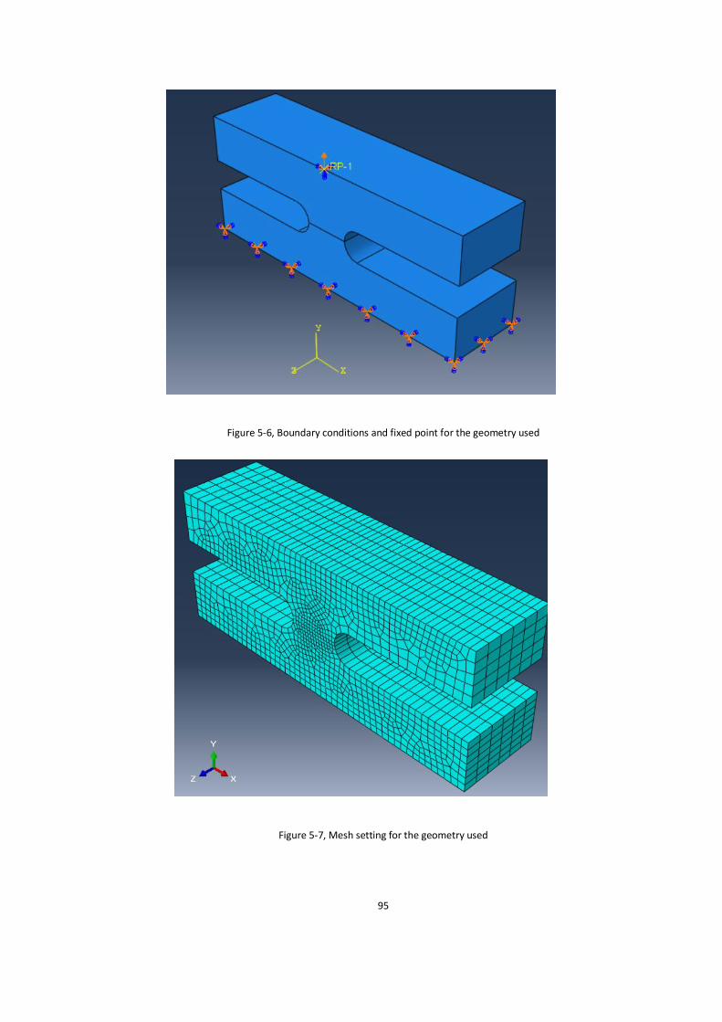
95

Figure 5-6, Boundary conditions and fixed point for the geometry used

Figure 5-7, Mesh setting for the geometry used

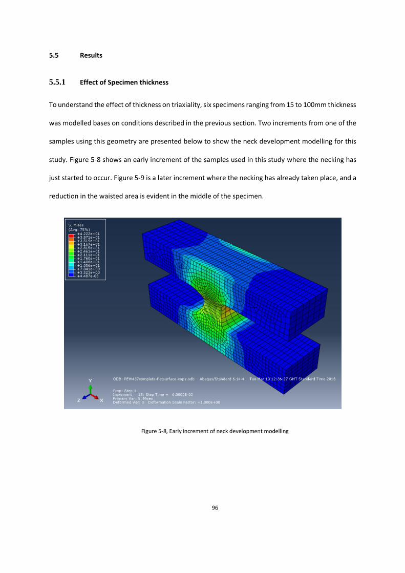
96

Results

5.5.1 Effect of Specimen thickness

To understand the effect of thickness on triaxiality, six specimens ranging from 15 to 100mm thickness

was modelled bases on conditions described in the previous section. Two increments from one of the

samples using this geometry are presented below to show the neck development modelling for this

study. Figure 5-8 shows an early increment of the samples used in this study where the necking has

just started to occur. Figure 5-9 is a later increment where the necking has already taken place, and a

reduction in the waisted area is evident in the middle of the specimen.

Figure 5-8, Early increment of neck development modelling

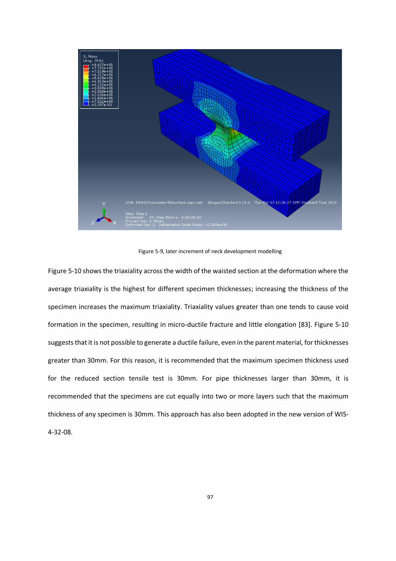
97

Figure 5-9, later increment of neck development modelling

Figure 5-10 shows the triaxiality across the width of the waisted section at the deformation where the

average triaxiality is the highest for different specimen thicknesses; increasing the thickness of the

specimen increases the maximum triaxiality. Triaxiality values greater than one tends to cause void

formation in the specimen, resulting in micro-ductile fracture and little elongation [83]. Figure 5-10

suggests that it is not possible to generate a ductile failure, even in the parent material, for thicknesses

greater than 30mm. For this reason, it is recommended that the maximum specimen thickness used

for the reduced section tensile test is 30mm. For pipe thicknesses larger than 30mm, it is

recommended that the specimens are cut equally into two or more layers such that the maximum

thickness of any specimen is 30mm. This approach has also been adopted in the new version of WIS-

4-32-08.

98

Figure 5-10, Variation of triaxiality across the width of the waisted section for specimens with different thicknesses (width

of the waisted section 25mm and radius of the waisted section 10mm)

The experimental tests to indicate the thickness effect were carried on 15 and 25mm thickness (from

Chapter 3). The Force-Deformation graphs for these two specimens are shown in Figure 5-11. The

dimensions used in these specimens are from BE EN 12814-7, which is shown in Figure 1-1.

99

Figure 5-11, Experimental Load-Displacement for 15 and 25mm thickness

In Figure 5-11, it can be seen that the yield point for 25mm thickness is higher than 15mm thick

specimen which is due to the larger CSA in the specimen. The cold drawing region in 15mm thick

specimen provides a long elongation which shows a high ductility in the specimen. The 25mm thick

specimen has failed to undergo cold drawing region and has started to fail from micro voiding growth.

Photos from the fracture surface of these two specimens are shown in Figure 5-25.

5.5.2 Effect of the width of the waisted section on triaxiality

To determine the effect of the width of the waisted section on triaxiality the same geometry

configuration as given in Figure 5-4 is used; however, the specimen thickness is kept constant at

25mm. This was selected purposely to have the failure due to void growth, which is from triaxiality.

The radius of the waisted section is kept constant at 5mm, and the width of the waisted section is

varied between 15 and 27.5mm.

This set of experiment is also carried out empirically by varying the width of the waisted section and

keeping other parameters constant.

100

The distance between loading holes also has some effects, but in this study, it has been considered to

have it close to its initial value and increase the amount that would be lost from an increase in loading

hole diameter. Loading hole diameter is adjusted to be equal to the width of the waisted section to

avoid elongation of the loading pinhole.

Figure 5-12 shows the variation of triaxiality factor across the width of the waisted section at the

displacement value where the average triaxiality is the highest for a 5mm radius of the waisted

section. From this figure, it can also be seen that for a 25mm thick specimen, the larger the width of

the waisted section is the lower the maximum triaxiality point is.

Figure 5-12, Validation of across the width of the waisted section for specimens with different widths of the waisted

section (wall thickness 25mm, the radius of the waisted section 5mm)

Recording the highest triaxiality point on the specimen during the tensile testing is essential as it is the

main factor to trigger the void formation. Void formation in the specimen would trigger the failure

and stops the cold drawing to take place.

101

In Figure 5-12, it can also be seen that the specimen with a 15mm width of the waisted section had

the most substantial triaxiality factor value. From 15mm to 27.5mm width of the waisted section, all

specimens have triaxiality values of over one except 27.5mm, where the maximum triaxiality point

reaches one and have the lowest triaxiality value across other specimens.

Figure 5-13 shows experimental tensile test specimen load-displacement curves for 25mm thick

specimens with different width of the waisted section specimens. 5 out of 6 specimens in this

experiment failed due to void growth. One specimen, which is PEW45 with 27.5mm width of the

waisted section is failed after going through a long cold drawing and failed from tearing.

Figure 5-13, Load-displacement curves on 25mm thick specimens varying the width of the waisted section

The experimental results shown in Figure 5-13 provides sufficient evidence for the effect of the

triaxiality on the failure of HDPE due to geometric effects.

102

The primary purpose of performing these modellings and experiments is to propose a new specimen

geometry for the geometry shown in Figure 1-1. The other parameter which would be used for the

investigation of triaxiality is the radius of the waisted section, which can be seen in the next section.

5.5.3 Effect of the radius of the waisted section on triaxiality

Effects of the thickness and width of the waisted section of the specimen are investigated in the last

two parts of this chapter. Taking into account the trends seen in the effect of the thickness and effect

of the width of the waisted section on failure behaviour, a similar analysis is carried on the radius of

the waisted section. To investigate the effect of the radius, four types of assessments are carried out

using radiuses of 5mm, 7.5mm, 10mm and 12.5mm accordingly. The result of this analysis is shown in

Figure 5-14, where the triaxiality factor for each point across the width of the waisted section is

recorded.

From Figure 5-14, it can be seen that the increase in the radius of the waisted section reduces the

maximum triaxiality during the test. Therefore, adjusting the radius is one of the geometry parameters

that can prevent failures occurring due to void growth in this scenario, the specimen with a radius of

5mm has the maximum triaxiality of 1.07, whereas the specimen with a radius of 12.5mm has a

triaxiality of 0.97.

103

Figure 5-14, Variation of triaxiality across the width of the waisted section for specimens with a different radius of the

waisted section (width of the waisted section 25mm)

It can be noted that specimens have the highest stress triaxiality at the centre of the specimen. This is

the location where the void grows and initiates the failure of the specimen. However, in a situation

where the thickness is larger or the width of the waisted section larger (than 30mm), then the areas

where the maximum triaxiality is high (over 1) is not only localised in the centre of the specimen, it is

also localised throughout the fracture surface. In this situation, the failure is not only due to one void

growth but also many other points on the fracture surface.

5.5.4 Effect of the width of the waisted section and loading hole diameter on elongation in the

loading hole

As the effect of the loading hole is being investigated from this study, changes were made to the

geometry. Figure 5-15 shows the boundary conditions and meshing for the geometry used in this

study; the Left figure shows the geometry configuration and the areas where partition has taken place.

104

As this geometry is 1/8th of the actual geometry, symmetric boundary conditions have been applied

on the surfaces and edges where the yellow dots indicate their separations. The top quarter of the

hole has been taken as the pin effect where displacement is used to pull the specimen. Overall meshed

geometry is on the right side of Figure 5-15 where partitions are used to produce a more dense mesh

area on the areas of interest. As the mesh is very dense on the waisted area it is shown separately in

Figure 5-16.

Figure 5-15, Boundary conditions and meshing used for determining the effect of the width of the waisted section on

elongation in the loading hole diameter

105

Figure 5-16, Detailed mesh configuration at the waisted area

To present the necking that occurred in these specimens, two geometries from early and later

increments of the modelling is presented in Figure 5-17 and Figure 5-18. This clearly shows the neck

development in the symmetric configuration used. This geometry and conditions are used in this

study to investigate the effect of wasited section on the elongation in loading hole for two cases. One

is when the pin is a constant value and the second case is when the pin diameter is changed with the

size of the waisted section.

106

Figure 5-17, Early increment of neck modelling using symmetry geometry

Figure 5-18, Later increment of neck modelling using symmetry geometry

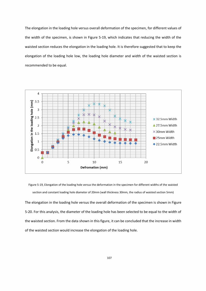
107

The elongation in the loading hole versus overall deformation of the specimen, for different values of

the width of the specimen, is shown in Figure 5-19, which indicates that reducing the width of the

waisted section reduces the elongation in the loading hole. It is therefore suggested that to keep the

elongation of the loading hole low, the loading hole diameter and width of the waisted section is

recommended to be equal.

Figure 5-19, Elongation of the loading hole versus the deformation in the specimen for different widths of the waisted

section and constant loading hole diameter of 20mm (wall thickness 30mm, the radius of waisted section 5mm)

The elongation in the loading hole versus the overall deformation of the specimen is shown in Figure

5-20. For this analysis, the diameter of the loading hole has been selected to be equal to the width of

the waisted section. From the data shown in this figure, it can be concluded that the increase in width

of the waisted section would increase the elongation of the loading hole.

108

Figure 5-20, Elongation of the loading hole versus deformation of the specimen for different widths of the waisted section

(wall thickness 30mm, the radius of waisted section 5mm, loading hole diameter same as the width of the waisted section)

5.5.5 Ductile and micro-ductile failure

As shown in Figure 5-21, an X-ray computed tomography (XCT) is used to observe the fracture surfaces

for PEW42&37 specimens. The motive behind applying XCT method is being able to scan and

investigate the fracture surface in 3 dimensions. To investigate the fracture surfaces of specimens

using XCT, unlike many other techniques, the surface is not required to be flat.

The XCT system used to obtain XCT scans during this study is an HMX 225 originally supplied by Metrix

X-Tek Ltd. The source, manipulator, detector and XCT data acquisition are controlled by X-Tek InspectX

software which digitizes the radiographic images to 16-bit format. One of the specimens in this

observation is PEW42 with the thickness of 25mm and width of the waisted section of 20mm with

failures from void growth in the centre of the specimen.

109

Figure 5-21, Xray photography of micro ductile failure for specimen number 42

The initial observation and analysis of the fracture surface show that the failure is due to one void, but

more in-depth visualisation lead through x-ray photography lead to the discovery of three central

voids mostly in the centre of the fracture surface. By zooming at the images found from X-Ray, at the

surface of the fracture surface in Figure 5-22, a large number of small circles (voids which have not

grown) could be seen, but most are in small dimensions which can be said that they have not been

triggered. This phenomenon and creation of these circles could be due to reaching a certain amount

of triaxiality, but few are triggered, which caused the failure, and the rest are not triggered entirely

due to the reduction of triaxiality value after the failure starts to happen.

110

Figure 5-22, X-Ray Photography of micro ductile failure for specimen number 42

The other type of failure mode occurs on specimens with different thicknesses (usually lower), and

different geometry configuration is the ductile failure, where the failure happens after the specimen

has gone through large deformation. The X-Ray photography of ductile failure can be seen in Figure

5-23 and Figure 5-24.

111

Figure 5-23, X-Ray photography of ductile failure for specimen no 37

Figure 5-24, X-Ray photography of ductile failure for specimen no 37

112

Figure 5-25, from left, fully ductile and micro ductile failure

The specimens used to carry out X-Ray for the demonstration of fully ductile and micro ductile failure

are shown in Figure 5-25. The difference between the fracture surfaces of these specimens is also

visible by visual inspections.

Conclusion

In this chapter, a summary of the techniques used to model polymers is compared and explained. The

constitutive model used in this study is explained with constants used in the equation revealed. A step

by step methodology is explained as to how the numerical modelling is set up and what criteria are

used for measurements in modelling.

Despite the possibility of modelling necking in the specimen, failure of the specimen could not be

modelled due to different challenges and complex failure mechanism of polymers. To be able to

113

compare the experiments in modelling, the triaxiality factor, which is an indication of the state of the

stress at a certain point, is used. As the maximum triaxiality is the point where it triggers the voids in

the specimen, triaxiality points at increments and locations with the highest triaxiality value are used.

Two types of failures seen in parent material specimens, ductile and micro ductile, are displayed from

experimental work carried out in previous chapter 3 and are related to triaxiality values found using

FE analysis. Two types of ductile failure modes are exposed and explained with in-depth X-Ray

photography, which explains these failures' reasons.

Using numerical modelling techniques, comparison against thickness, width and radius of the waisted

section of the specimen are carried out and compared with their triaxiality stress state in the middle

of the specimen. Elongation in the loading hole diameter against the width of the waisted section and

loading hole diameter is also investigated.

This part of the research suggests that for specimens with a thickness of over 30mm, the triaxiality

factor would be around the value of one, which means any specimen with a thickness of over 30mm

would have a high chance of failing from void growth in the specimen. An increase in width and radius

both reduces the triaxiality factor, but the study suggests there should be a limit to the increase as

this would affect the elongation in the loading hole as well as where the failure in the specimen takes

place.

114

Chapter 6. Proposed specimen geometry and its

application on welded and unwelded HDPE pipes

Chapter overview

In this chapter, an enhanced geometry is proposed, experimentally tested, and been applied to

different pipes with different thicknesses having welded and unwelded conditions. This chapter also

clarifies the motives for selecting specific pipe sizes. Welding parameters, as well as the location of

each sample on the pipe, is also explained.

Introduction

In previous chapters, the effect of different parameters on waisted tensile geometry was investigated

both experimentally and using FEA analysis techniques. The principal reason to conduct this research

is to identify a geometry that can be utilised to quantify the quality of butt fusion joints for different

thicknesses and provides useful quantitative information to allow discrimination among different weld

qualities. Standard geometry using a flat sheet for the thickness of 25mm is tested in Chapter 3, which

showed that a fully ductile failure could not be achieved, and the specimens with 25mm thickness

failed from void growths. The benefits of the proposed modified geometry are confirmed after the

comparison provided against the standard geometry.

For each condition (each weld and pipe size), few samples (4-5-6) using standard and proposed

modified geometry have been machined and tested at different angles of the pipe to investigate all

factors which could affect the results.

115

Finally, the results are compared, and the effect of different pipe sizes will also be investigated using

both current standard geometry (BS-EN 12814-7) as well as the proposed enhanced geometry.

Designed geometry for different thicknesses

FEA results revealed the challenges of generating a ductile fracture in a reduced section specimen for

specimen thicknesses greater than 30mm. This challenge is present for both flat specimens and

specimens cut from the parent pipe. This means that for thicknesses greater than 30mm, it can be

difficult to differentiate between good and bad welds using this test method.

Since all specimens fail in a brittle (micro ductile) manner, it is therefore suggested that, for pipe wall

thicknesses greater than 30mm, the specimens are cut equally into two or more layers such that the

maximum thickness of the specimen is 30mm.

Based on the DOE study (provided in chapter 4), increasing the radius of the waisted section increases

the energy to break the specimen. This means, the triaxiality factor reduces as the radius increases

and also it is highly likely that failures occur outside of the weld region in a welded specimen.

Therefore, it is recommended to use a radius of 10mm for the waisted section in different scenarios.

The DOE study, as well as the work carried out in chapter three, suggested that for a specimen with

15mm thickness, the width of the waisted section should be equal to the specimen’s thickness in order

to achieve higher energy to break value (specifically Region 3 energy). The FEA study suggested that

for a specimen with 30mm thickness, the width of the waisted section should not be less than the

specimen thickness in order to achieve a low triaxiality factor. However, increasing the width of the

waisted section also increases the elongation in the loading hole. Therefore, it is suggested that the

width of the waisted section of 30mm should be used for 30mm thick specimen.

116

The DoE study on 15mm thick specimens suggests that a loading hole diameter of 20mm will give the

highest energy to break. However, for 30mm thick specimens, the FEA suggests that, in order to

reduce the elongation in the loading hole, it is better to keep the loading hole diameter equal to the

width of the waisted section, i.e. 30mm.

The DoE study on 15mm thick specimens suggests that the energy to break increases as the distance

between the loading hole increases. This is due to the decrease in strain rate at the waisted region.

The suggested distance between the loading holes for a 15mm thick specimen with a diameter of

20mm is 100mm. Therefore, the suggested distance between the loading holes for a 30mm thick

specimen, with a diameter of 30mm is 110mm, to compensate for the larger diameter.

From the DoE study on 15mm thick specimens, the energy to break increases as the overall width of

the specimen increases. There have to be limits on how much the width can be increased. This limit

is set not to have the specimen being failed or elongated from the side of the specimen. Therefore,

the proposed overall width for specimens with thickness of lower than 20mm, between 20 to 25mm

and between 25 to 30mm are 70, 80 and 80mm, respectively.

Based on these results, the proposed optimised geometry of 30mm thick reduced section specimens

is given in Table 6-1, where it is compared with the geometry specified in WIS 4-32-08-2017.

117

Figure 6-1, reduced section specimen related to the table below

Table 6-1, Dimensions for reduced section specimen geometry given in WIS 4-32-08:2-17 and the proposed optimised

geometry from this study

Symbol Description WIS 4-32-08 Enhanced Geometry

(For 30mm Thickness)

A Overall length (mm) ≥180 210

B Overall width (mm) 80 80

C The distance between loading holes (mm)

90 110

D Width of waisted section (mm) 25 30

E The diameter of loading holes (mm)

20 30

F The radius of the waisted section (mm)

10 10

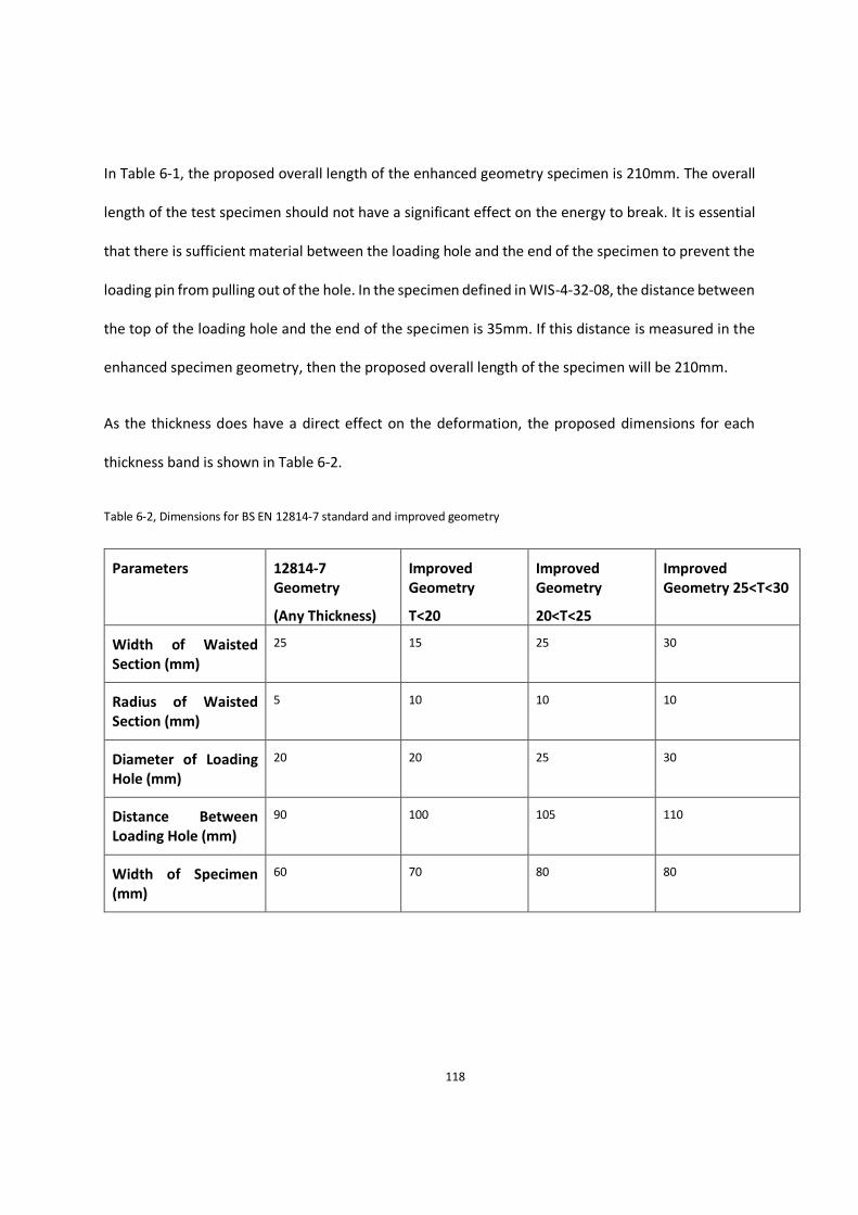
118

In Table 6-1, the proposed overall length of the enhanced geometry specimen is 210mm. The overall

length of the test specimen should not have a significant effect on the energy to break. It is essential

that there is sufficient material between the loading hole and the end of the specimen to prevent the

loading pin from pulling out of the hole. In the specimen defined in WIS-4-32-08, the distance between

the top of the loading hole and the end of the specimen is 35mm. If this distance is measured in the

enhanced specimen geometry, then the proposed overall length of the specimen will be 210mm.

As the thickness does have a direct effect on the deformation, the proposed dimensions for each

thickness band is shown in Table 6-2.

Table 6-2, Dimensions for BS EN 12814-7 standard and improved geometry

Parameters 12814-7 Geometry

(Any Thickness)

Improved Geometry

T<20

Improved Geometry

20<T<25

Improved Geometry 25<T<30

Width of Waisted Section (mm)

25 15 25 30

Radius of Waisted Section (mm)

5 10 10 10

Diameter of Loading Hole (mm)

20 20 25 30

Distance Between Loading Hole (mm)

90 100 105 110

Width of Specimen (mm)

60 70 80 80

119

Pipe Sizes

To compare the modified geometry with the current standard’s geometry using welded specimens,

pipes with different dimensions had to be prepared. The requests on quotations were to have all the

pipes from the same resin batch and the length to be around 2 meters. Suppliers informed to have

resins from one batch is not possible, and the minimum order quantity is 5 meters for each pipe size

requested. The main task after finding the right manufacturer was to start the selection process with

the least number of pipes and have the maximum combination for different factors. The main factor

in this study is the thickness of the pipe, and therefore while selecting the pipe sizes, it is assumed to

have a full range of thicknesses. The other factor is to understand the effect of curvature for the pipe,

and that is shown with the standard dimension ratio SDR (ratio of the outside diameter to the wall

thickness of the pipe) of the pipe.

The pipe dimensions selected for this study are shown in Table 6-3. The thicknesses selected starts

from 12.7mm to 57.3mm with an outer diameter of 140mm to 630mm. Pipe sizes with an outer

diameter of 160mm and 250mm were explicitly used to have a similar thickness (closest thickness

among available pipe sizes) to precisely compare the SDR of the pipe. The other pipe sizes were mainly

to check the effect of the thickness except for 140 and 160mm, which provide the closest outer

diameter but different thicknesses.

Table 6-3, Pipes used for this study with their dimensions and welding machines used

Outer Diameter (mm)

SDR Thickness (mm)

No of Welds

Welding Machine

140 11 12.7 4 BF315

160 11 14.5 4 BF315

250 17 14.7 2 BF315

280 11 25.5 2 BF315

500 11 45.5 2 Mc1236

630 11 57.3 2 Mc1236

120

Butt Fusion Welding

As mentioned in the literature review section, the principle of the fusion welding technique is to melt

two pipe surfaces sufficiently so that molecular segments can diffuse across the contact surface and

form bonds in which extend to provide a joint with comparable strength to the parent component.

For joining pipes with an outer diameter of lower than 250mm, butt fusion and electrofusion

techniques could be used. For PE pipes with an outer diameter greater than 250mm, butt fusion

welding is the primary technique, and it is the only technique available for pipes greater than 500mm

outer diameter.

The steps for butt fusion welding is shown below in Figure 6-2, Schematic diagram of the pressure

cycle during the butt fusion welding process with a few steps before starting this welding procedure.

The first step of the welding procedure is placing pipes into the clamp of the butt fusion machine and

check for alignment. The next step is trimming the pipe ends to ensure they are flat and square. After

these two steps, the primary procedure starts by applying the heater plate and increasing the pressure

to reach the bead-up pressure, where the schematic diagram of the pressure cycle is shown in Figure

6-2.

121

Figure 6-2, Schematic diagram of the pressure cycle during the butt fusion welding process)

To carry out a butt fusion welding, similar welding machine procedures and welding processes apply

to pipes with different outer diameter and thicknesses, but the factors such as time, hydraulic pressure

and temperature of the heater plate are entirely based on the dimensions and thickness of the pipe.

The standard followed to carry out the welding for this research is DVS 2207-1. As mentioned in the

introduction section and shown in the diagram above, the process after alignment and trimming is

divided into bead-up, heat soak, changeover and finally joining or fusion.

The bead-up step starts with pressing the pipe surfaces to the heated tool, and it is carried out to

make sure all angles and surface area of the pipe is pressing the heated tool. This process is carried

out by measuring the bead height. When the bead height has reached an absolute value (0.5mm for

pipes up to 355mm and 1mm for pipes with an outside diameter of 400 and 630mm according to DVS-

2207-01, Table 8-15 ), it is an indication that the joining areas are all in contact with the heated tools.

122

The heat-soak or heating-up stage takes place after the confirmation of full contact between the

joining area and the heater plate. The pressure for this process is reduced to zero and the time varies

based on the thickness of the pipe.

After completing the heating-up stage, the heated tool should be withdrawn from the welding

machine without causing any damage or contamination to the heated joining zones. The changeover

stage must take place as quick as possible. Otherwise, the plasticised area will be cooled down. The

quality of the weld will be highly be influenced if this procedure is not carried out on the targeted time

given in Table 6-4.

Table 6-4, Recommended values for the heated tool butt welding of pipes (DVS-2207-01)

The joining or fusion stage takes place when the joining area is pressed together, starting with very

low pressure and once reached each other; the pressure increases linearly to 0.15N/mm2. The joining

pressure must be constant during the cooling time (mentioned in Table 6-4). After the cooling time,

the pressure can be released, and the pipe with the joint can be removed from the welding machine

only if very slight loads applies to the weld.

123

Welding reports have been prepared for each well and are available for each pipe diameter.

Pipe with 140mm outer diameter

The first set of experiments were carried out using pipes with 140mm outer diameter. The welding

was carried out using a BF315 welding machine, where the welding machine has different advantages

and disadvantages.

An advantage of the machine is its automatic feature, where after placing the pipes and selecting

welding standard with the right pipe diameter, the welding process can be carried out automatically.

However, this automatic feature has a drawback, where each weld is required to be fully completed

before starting a new weld. This made the process of dummy welds (used to clean contamination from

a hot plate) time-consuming. The only manual works required for this machine is to replace the

trimmer with a heater over the welding machine, and the rest of the welding process is carried out

automatically.

The primary purpose of these experiments is to compare the standard geometry with the enhanced

geometry for welded pipes as well as parent material cut from the pipes. To assure the reliability of

the data, for every pipe size, a minimum of 5 repeated specimens for every condition is tested. For

every weld or parent pipe, the experiment is designed to cut the modified and standard geometry at

adjacent positions. For this case, as the outer diameter is 140mm, a maximum of four specimens could

be taken from each weld or parent pipe. The position of each specimen with specimen numbers is

provided in Appendix part D (Table 8-9).

The standard and modified geometry dimensions for this set of the experiment are shown in Figure

6-3.

124

Figure 6-3, Modified geometry on the left used for thicknesses less than 20mm vs standard 12814-7 geometry on the right

The comparison of 140mm pipe for a specimen that is cut from parent pipe material, using standard

and modified geometry is shown in Figure 6-4. The graph shows the force-deformation data for both

specimens. As the CSA of specimens is different, there is a significant difference in the maximum loads

of specimens. The cold drawing region in the modified specimen is much higher than the standard

specimen. This proves higher ductility for unwelded modified geometry specimen compared to

unwelded standard geometry specimen. The other advantage of the modified specimen geometry is

the necking at earlier stages of the test, compared to the standard geometry. When the necking occurs

125

in earlier stages of the deformation, it is an indication of lower elongation throughout the specimen

surface (lower elongations in loading hole diameter), and deformations are likely taking place in the

waisted area of the specimen. The fracture surfaces of these two specimens are shown in Figure 6-5,

which shows longer elongation for the modified specimen geometry. As discussed in previous

chapters, longer elongation is desirable in this application due to providing a suitable condition for the

welded area to be assessed.

Figure 6-4, Force-Deformation graph for modified and standard geometry on unwelded 140mm OD pipe

126

Figure 6-5, Fracture surface of the parent standard on the left and parent modified geometry on the right from 140mm OD

pipe

As the CSA is different for the mentioned specimens, the force is divided by the CSA to provide nominal

stress and allow a uniform comparison condition (Figure 6-6). In this figure, it is shown how the

modified geometry has improved the deformation in the specimen comparing to the standard

geometry. Necking also starts at an earlier stage which is a great indication of lower elongation in

holes.

Parent, Standard

Parent, Modified

127

Figure 6-6, Nominal stress-Deformation graph for modified and standard geometry on unwelded 140mm OD pipe

The next set of comparison shows the two specimens (modified and standard) from welded pipes.

Their positions are adjacent to each other on the pipe to minimise uncertainties affecting the result

of the tensile tests introduced by heater plate or extrusion machines. In both specimens, cold drawing

region has disappeared, which is due to having an additional material with different material property

(weld) as well as the effect of the shape produces by the beads (Figure 6-7).

The fracture surfaces shown in Figure 6-8 indicate ductility for both modified and standard geometry

with elongations in both cases. Specimens that have formed one of the welded pipes, including two

modified and two standard geometry, are shown in Figure 6-9, and ductility can be confirmed in all

cases.

128

Figure 6-7, Nominal stress-Deformation graph for modified and standard geometry on welded 140mm OD pipe

Figure 6-8, Fracture surface of the welded standard specimen on the left and welded modified specimen geometry on the

right from 140mm OD pipe

Welded, Standard

Welded, Modified

129

Figure 6-9, From Left, the fracture surface of standard, modified, standard and modified specimen geometry from 140mm

OD welded pipe

For 140mm OD welded pipe, one experiment is carried out where the weld beads are removed

internally and externally. The comparison graph for modified and standard geometry specimens from

welded pipes without beads are shown in Figure 6-10. Cold drawing region can be observed in the

graph, which confirms the effect of the beads on the specimen. Taking beads off from the welded

pipes has led to more elongation in both specimens using both standard and modified geometry. The

fracture surfaces for these specimens are shown in Figure 6-11. Comparison of these fracture surfaces

indicates a longer elongation in the welded area for modified specimen geometry, despite a more

extended deformation in the tensile test for the whole standard geometry.

Welded, Standard

Welded, Standard

Welded, Modified

Welded, Modified

130

Figure 6-10, Nominal stress-Deformation graph for modified and standard geometry on welded with beads off on 140mm

OD pipe

Figure 6-11, Fracture surface of the welded standard specimen on the left and welded modified specimen geometry on the

right from 140mm OD beads off pipe

Welded, Standard, No Beads

Welded, Modified, No Beads

131

Total energy per CSA for different conditions of 140mm OD SDR 11 pipe is shown in Figure 6-12. The

conditions shown are; standard and modified specimen using the unwelded welded and welded pipes

with no beads. Each bar represents the average of five samples, with error lines representing the

standard deviation for the five repeated experiments carried out for 140mm OD pipes.

From Figure 6-12, it can be seen that the modified specimen using unwelded pipe provides the

maximum total energy per CSA. When comparing the specimens with the welded condition, the

modified geometry did not provide higher total energy compared to the standard geometry specimen.

However, as can be seen in the graph, the energy indicated in the modified geometry test is a better

indication of the energy consumed in the waisted area of the specimen. On conditions where beads

are taken off, the total energy is higher compared to the welded with beads, despite removing the

extra material from around the welded area. This can be due to a more uniform cross-sectional area

of the specimen, which allows longer necking.

Figure 6-12, Total Energy per CSA for different scenarios on 140mm OD SDR 11 pipe

132


Similar to 140mm OD pipes, welding is carried using a BF315 welding machine. The modified geometry

for lower than 20mm is the geometry used for specimens with a thickness of lower than 20mm.

The first comparison is provided for a standard against modified geometry using unwelded pipe

specimens (Figure 6-13). The specimen with modified geometry provides a much larger elongation

compared to standard geometry, which is more desirable in this application.

Figure 6-13, Nominal stress-Deformation graph for modified and standard geometry on parent 160mm OD pipe

The next comparison is provided for modified and standard specimen geometry for 160mm OD

welded pipes. From the graph in Figure 6-14, necking starts after ~ 7.5mm deformation on the

modified specimen, whereas the necking starts after about 16mm deformation on the standard

geometry. This suggests that, despite the larger area under the curve (energy consumption) for

133

standard geometry, the data in modified geometry represent the energy consumed are mainly in the

area of interest (waisted region of the specimen).

The fracture surfaces for standard and modified geometry of 160mm OD welded pipe is shown in

Figure 6-16. For four cases of parent and welded specimen using standard and modified geometry,

comparison of the average energy per CSA for these different conditions are shown in Figure 6-15.

Modified specimen provided the largest energy to break value, and welded modified specimen

provided lower total energy compared to the standard geometry. However, it is a better indication of

energy consumed in the welded area due to necking initiating at earlier stages of the tensile test.

Figure 6-14, Nominal Stress-Deformation graph for modified and standard geometry on welded 160mm OD pipe

134


Figure 6-16, Fracture surface of the welded modified specimen on the left and welded standard specimen geometry on the

right from 160mm OD pipe

Welded, Modified

Welded, Standard

135


This experiment is carried out on 250mm SDR 17 pipes which are the only pipes with SDR 17 in this

study, whereas the other pipes are SDR11. Similar to 140mm and 160mm OD pipes, the geometry for

specimens with a thickness of less than 20mm is used against the standard geometry. The experiment

is carried out on both the unwelded and welded pipes. Welding is carried out using the BF315

machine. The result for the unwelded specimen is similar to 140mm and 160mm OD pipe cases. The

modified geometry has larger elongation and earlier necking stage compared to the standard

geometry (Figure 6-17).

Figure 6-17, Nominal stress-Deformation graph for modified and standard geometry on parent

250mm OD pipe

Figure 6-18, which confirm longer elongation in modified geometry. For welded case, similar to

140mm and 160mm pipes, the necking started in much earlier stages compared to the standard

geometry, which means again, the energy for the modified geometry is mainly consumed to elongate

the waisted area (Figure 6-19). Fracture surfaces of these conditions are shown in Figure 6-21, in which

136

all fracture surfaces pass the welding criteria and count as ductile failure. Figure 6-20 shows the

comparison of energy to break values for different cases with more considerable value for parent

modified condition, which is approximately twice as the standard parent material. The standard

deviation value is at its highest for parent modified, which indicates the differences between energy

to break the value of specimens.

Figure 6-18, From left, fracture surface of standard, standard, modified and modified specimen geometry on 250mm OD

parent pipe

Parent, Standard

Parent, Standard

Parent, Modified

Parent, Modified

137

Figure 6-19, Nominal stress-Deformation graph for modified and standard geometry on welded 250mm OD pipe


138

Figure 6-21, From left, fracture surface of modified, modified, modified, standard, standard and standard specimen

geometry on 250mm OD welded pipe


For 280mm OD pipe, the wall thickness is ~ 25.5mm. Therefore the modified geometry for a specimen

with a wall thickness of between 25mm to 30mm is used. The standard geometry next to the modified

geometry used for this set of the experiment can be seen in Figure 6-22. As it was mentioned in

previous chapters, thickness is one of the main factors affecting the failure modes of the specimen.

Welded, Modified

Welded, Standard

139

Figure 6-22, from left to right, standard and modified geometry used for thickness in between 25mm and 30mm

When the tensile test is applied to the standard specimen on the unwelded pipe situation, the

specimen did not experience any elongation or cold drawing and resulted in a rapid failure after

necking. In opposite, the modified geometry did go through a complete cold drawing region and failed

from tearing (shear yielding) at the end of the test (Figure 6-23). This highlights the standard geometry

challenges where ductile failures do not occur despite using unwelded parent material. As discussed

in the introduction, this standard has been used in industrial applications for a long time; however,

this geometry is not necessarily providing useful information about the weld's quality. Our proposed

modified geometry overcomes this challenge by providing desirable ductile failures in all parent pipe

specimens.

140

Figure 6-23, Nominal stress-Deformation graph for modified and standard geometry on parent 280mm OD pipe

The same geometries are applied to the welded specimen, where the comparison is shown in Figure

6-24. As expected in welded condition, the specimen with standard geometry failed just after the

necking point, whereas the modified geometry had more drawing before the failure. The fracture

surface for this condition is shown in Figure 6-25, where more ductility can be seen on the modified

geometry. From the fracture surface of these specimen in Figure 6-25, the fracture surface of the

specimen using standard geometry does not contain any yielding or drawing in its surface and contains

large number dots, which have been the points of failure for this specimen geometry. By checking

these two fracture surfaces, it is clear that the failure mechanism for these specimens is different. Two

more specimens from the same pipe and weld are shown for 280mm pipes which are Figure 6-28 and

Figure 6-29.

141

Figure 6-24, Nominal stress-Deformation graph for modified and standard geometry on welded 280mm OD

Figure 6-25, Fracture surface of the welded standard specimen on the left and modified welded geometry on the right from

welded 280mm OD pipe

Welded, Standard

Welded, Modified

142

For both conditions of the welded and unwelded specimen, five samples are selected for each

geometry. The chart given in Figure 6-26 shows that the modified geometry for both conditions has

higher energy to break values compared to the standard geometry. Unwelded condition using

modified geometry provided the most substantial energy to break value, which is approximately twice

as the energy to break for standard geometry on unwelded parent pipe. As expected, the welded

specimen using the standard geometry has the lowest energy to break value which can be seen in the

graph provided as well as their fracture surfaces.


Fracture surfaces for welded 280mm OD pipes are shown in Figure 6-27. As mentioned earlier, the

position for each specimen is selected to have the standard and modified geometries adjacent to each

other in a particular weld or pipe. As can be seen in Figure 6-27, the specimen with wider widths are

the specimens with modified geometries, which indicates more elongation at their fracture surfaces

compared to the standard geometry (Figure 6-28).

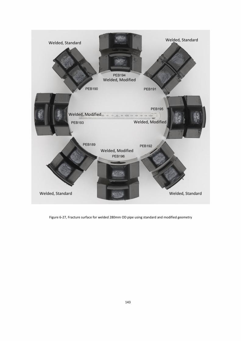
143

Figure 6-27, Fracture surface for welded 280mm OD pipe using standard and modified geometry

Welded, Modified

Welded, Modified

Welded, Modified

Welded, Modified

Welded, Standard

Welded, Standard

Welded, Standard

Welded, Standard

144

Figure 6-28, Fracture surface of modified welded specimen from 280mm pipe (PEB195)

Looking at the specimen (PEB 191) at one o’clock position shown in Figure 6-27, which is a standard

(BS EN 12814-7) geometry, it can be seen that the specimen did not experience any elongation and

the fracture surface is entirely flat. This brittle fracture surface does not repeat for the neighbouring

specimens (PEB 194 &195), as modified specimen geometries are used. This also proves that the

fracture surface of (PEB 191, Figure 6-29) exhibits poor/flat condition, which is not representing the

quality of the weld, as changing the specimen geometry (modified geometry) has fully transformed

the fracture surface of the specimens from the same weld.

145

Figure 6-29, Fracture surface of standard welded specimen from 280mm pipe (PEB191)


For 500mm OD pipes different welding machine, called MC1236, is used. Welding for 500 and 630mm

pipes was one of the most challenging tasks in this research. Operating the machine required extensive

training by McElroy Manufacturing. Pipes were placed and removed from the welding machine using

a 5-ton overhead crane. Some of the welding steps using this machine are shown in Figure 6-30.

146

Figure 6-30, From top left clockwise, Trimming, pipe position in the machine, heater plate in place, final weld

Each weld for 500mm and 630mm pipe diameters provide enough number of specimens for the

experiment (more than 10), but for assurance, two welds are produced for each pipe size. Welding

reports with corresponding graphs are available in Appendix D.

Thickness for 500mm OD Pipe is 45.5mm, therefore as WIS-32-04-08 standard suggested and findings

presented in chapter 5 recommended, the modified geometries for this experiment are cut to half

from the middle. It is also discussed in chapter 5 that specimen with a large thickness (over 20mm)

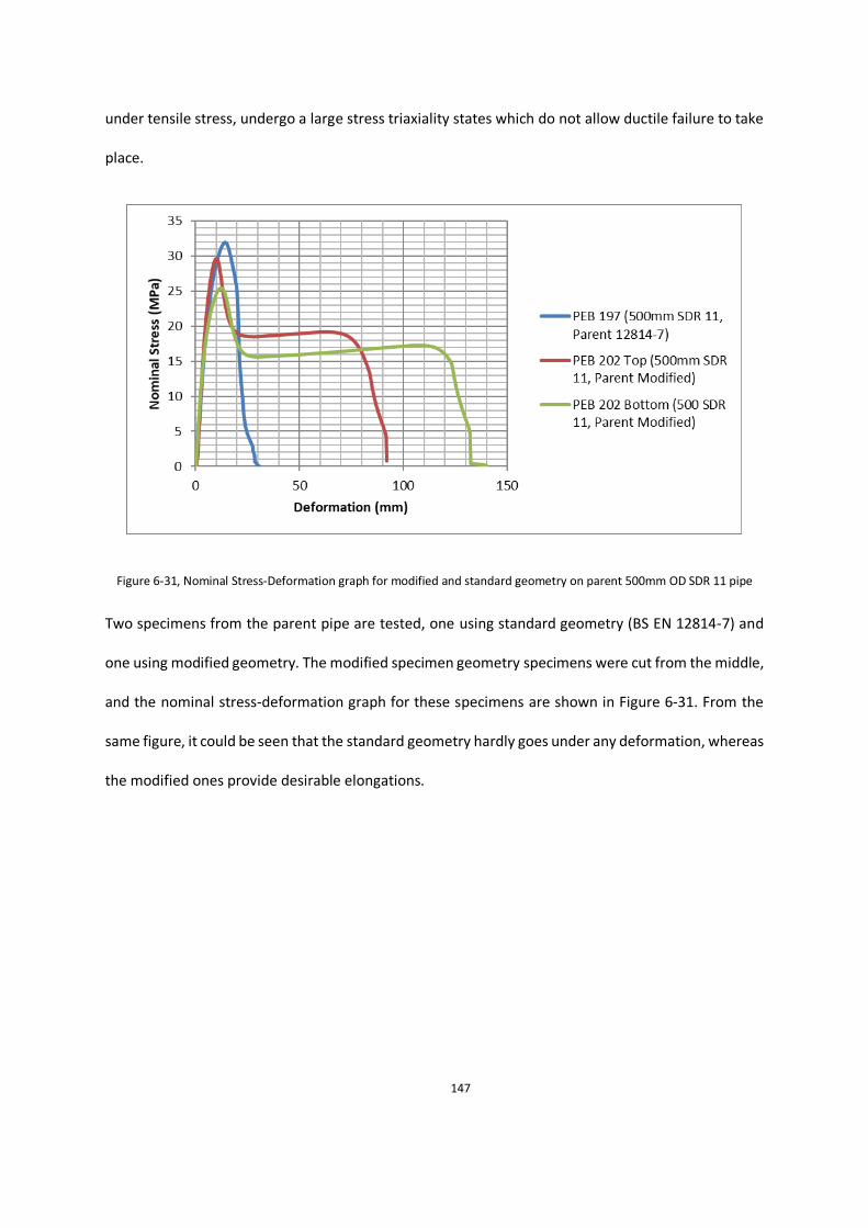
147

under tensile stress, undergo a large stress triaxiality states which do not allow ductile failure to take

place.

Figure 6-31, Nominal Stress-Deformation graph for modified and standard geometry on parent 500mm OD SDR 11 pipe

Two specimens from the parent pipe are tested, one using standard geometry (BS EN 12814-7) and

one using modified geometry. The modified specimen geometry specimens were cut from the middle,

and the nominal stress-deformation graph for these specimens are shown in Figure 6-31. From the

same figure, it could be seen that the standard geometry hardly goes under any deformation, whereas

the modified ones provide desirable elongations.

148

Figure 6-32, Nominal stress-Deformation graph for modified and standard geometry on welded 500mm OD

A similar procedure and specimen geometries are used for welded pipes. The nominal stress-

deformation graph for these two specimens is shown in Figure 6-32, which exhibit little elongation for

the standard geometry with a sharp drop in force absorbed by the specimen. The modified geometries

provide some elongation which can be confirmed using fracture surface photos provided later in this

chapter (Figure 6-36).

149


Energy per CSA for different conditions of 500mm OD SDR 11 is shown in Figure 6-33. Modified

geometry in an unwelded situation provides the maximum energy per CSA on average. Modified

geometry also provides more considerable energy per CSA compared to welded standard geometry,

as expected.

Fracture surfaces of modified and standard geometry for unwelded 500mm OD SDR 11 pipe are shown

in Figure 6-34 and Figure 6-35. The fracture surfaces for parent material using standard geometry

shows that the specimen was failed due to void growth and had limited elongation before the

specimen failed entirely. The fracture surface for the modified geometry on parent material indicates

yielding and elongation, which has led to having more energy to break the specimen and indicates a

ductile failure.

150

Figure 6-34, Fracture surface for parent 500mm OD SDR 11 pipe using standard and modified geometry

Parent, Standard

Parent, Standard

Parent, Standard

Parent, Standard

Parent, Standard

Parent, Modified

Parent, Modified

Parent, Modified

Parent, Modified

151

Figure 6-35, Fracture surface for parent modified specimen on the left (PEB204) and parent standard specimen

on the right (PEB197) from 500mm OD pipe

Fracture surfaces of modified and standard geometry for welded 500mm OD SDR 11 pipe are shown

in Figure 6-36 and Figure 6-37. It can be seen that on specimens where the standard geometry has

been used, there is minimal deformation and specimen are broken off from the middle with an entirely

flat surface which is undesirable. This study suggests the modified geometry experienced necessary

elongations to provide useful, measurable data about the quality of the weld as opposed to the

standard geometry, which provides little evidence for the quality of the welded joint.

152

Figure 6-36, Fracture surface for welded 500mm OD pipe SDR 11 using standard and modified geometry

Welded, Modified

Welded, Modified

Welded, Modified

Welded, Modified

Welded, Modified

Welded, Standard

Welded, Standard

Welded, Standard

Welded, Standard

153

Figure 6-37, Fracture surface for welded modified specimen on the left (PEB213) and welded standard specimen

on the right (PEB206) from 500mm OD pipe and from the same weld


630mm OD SDR 11 pipe was the largest pipe size in diameter and thickness, which is experimented in

this chapter. A similar welding machine as 500mm OD SDR 11 pipe (MC 1236 machine) is used for this

pipe size diameter. The pipe was cut to half as the length of the pipes was 5 meters for each pipe size,

which had to be welded. This was carried using a hand drill and jigsaw manually. The industrial saws

available are not used as they are all used previously to cut metal pieces and are contaminated.

154

For unwelded parent pipe specimens, the standard specimen geometry is tested in full-thickness, and

after being tensile tested, the specimens are failed with no elongation or ductility. Specimens with

modified geometry are cut into half from the thickness, and after being tensile tested, they provided

elongation in tensile tests which are shown in Figure 6-38.

The same geometry and procedure are used for the welded specimen. Specimens with standard

geometry are failed with no elongation at the welded area of the specimen, and the specimen with

modified geometry provided some elongations. The nominal stress-deformation graph for these

specimens is shown in Figure 6-39.

Figure 6-38, Nominal stress-Deformation graph for modified and standard geometry on parent 630mm OD SDR11 pipe

155

Figure 6-39, Nominal Stress-Deformation graph for modified and standard geometry on welded 630m OD SDR11 pipe


Energy per CSA for different conditions in 630mm OD SDR 11 pipe is shown in Figure 6-40. As expected,

the largest average energy to break was for parent modified condition. For welded condition, the

modified geometry also provided more sustainable energy to break value and from the specimen

156

geometry and fracture surface after the tensile test. It can be seen that most of the energy

consumption for standard geometry are for areas throughout the specimen and not the welded area.

Figure 6-41, Fracture surface for parent 630mm OD pipe SDR11 using standard and modified geometry

Parent, Modified

Parent, Modified

Parent, Modified

Parent, Modified

Parent, Modified

Parent, Standard

Parent, Standard

Parent, Standard

Parent, Standard

Parent, Standard

157

Figure 6-42, Fracture surface for parent 630mm OD pipe SDR 11 using standard on the right and modified geometry

on the left

The fracture surfaces for parent 630mm OD pipes are shown in Figure 6-41. It is clear that the

specimens with standard geometry are failed from micro void growth (PEB 220-219-218-217-216).

Specimens with modified geometry experienced large elongations and failed from tearing (shear

yielding) after complete elongation. Some of the specimens at the inner section of the pipe, despite

tensile elongations, had single void growth (Figure 6-42), which might be due to the way the large-

diameter pipes are cooled down in extruders.

Parent, Modified

Parent, Standard

158

Figure 6-43, Fracture surface for welded 630mm OD pipe SDR 11 using standard and modified geometry

The fracture surfaces for welded 630mm OD pipe are shown in Figure 6-43. Welded specimen with

standard geometry shows very little ductility, and as seen in 500mm OD pipe, the fracture surfaces

are flat (PEB 230, 229, 228, 227, 226). The specimens with modified geometry provided some

elongations, but as can be seen, the inner specimens provided less ductility both in the welded and

unwelded situation (Figure 6-44).

Welded, Standard

Welded, Standard

Welded, Standard

Welded, Standard

Welded, Modified

Welded, Modified

Welded, Modified

Welded, Modified

Welded, Modified

Welded, Standard

159

Figure 6-44, Fracture surface for welded modified specimen on the left (PEB233) and welded standard specimen

on the right (PEB226) from 630mm OD pipe and from the same weld

160

Comparison of Welding Factors

Welding factor, which is the ratio of total energy to break value of welded specimen against parent

material, are calculated and compared for the modified and standard geometry. Figure 6-45 shows

the welding factor for all pipe size diameters used in this experiment which are 140, 160, 250, 280,

500, 630mm OD.

Figure 6-45, Welding factors for different pipe sizes

In this chapter, modified geometries are proposed, which exhibited superior performance compared

to the standard geometry (BS EN 12814-7) regarding elongation in parent pipe specimens. This

improvement has led to a reduction in the value of the welding factor for modified geometry.

The reason for modified geometry to have a lower welding factor is having welded specimen using

modified geometry to start necking at earlier stages of the test. This means although more

considerable energy to break value for some welded specimen using standard geometry, the energy

for the modified specimen is a better indication of the energy consumed to elongate the welded area.

161

Conclusion

In conclusion, in this chapter, three different modified geometries (thickness related) were proposed

based on the findings of works carried out in chapters 3, 4 and 5. The reason behind the selection of

different pipe sizes and welding machines used were explained in this chapter.

The main work carried out was to compare the performance of the modified geometry to the standard

geometry (BS EN 12814-7) on different pipe sizes using parent and welded pipes.

It was shown that the modified geometry could differentiate the quality of the weld in all selected

pipe sizes producing the right failure (ductile) and not allowing the test to fail from micro voids. The

other advantage of the modified specimen is to have all failures occur in the welded area, which helps

to have a more accurate reading for energy to break value of the specimen.

The failure comparison of specimens on modified and standard geometry in this chapter was carried

from the same weld. The position of each modified and standard geometry was adjacent to each other

in order to minimise uncertainties (weld quality, the position of the specimen on the pipe) which might

affect the measurements. Despite all these conditions and having specimens (both standard and

modified geometry) from one weld, it is seen on 280, 500 and 630mm OD pipe specimen using

standard geometry have entirely flat fracture surface, where according to BS EN 12814-7 standard,

this count as a cold weld. Assessing the weld using modified geometry provided elongation on the

fracture surface, which proves the weld passes the criteria to be counted as a good weld.

162

Chapter 7. Conclusions and future works

Main findings of this thesis

The aim of this research was to investigate and improve the current standard geometry in quantifying

the quality of welds in HDPE pipes. A comprehensive literature investigation, series of laboratory

experiments (tensile tests, X-ray, DIC) were carried out to study the current standard geometry

problems. The problem with the current standard is that the same waisted tensile test specimen

geometry is used for all thicknesses. As stated in recent literature, when specimen thickness increases,

ductility decreases and because of this change, the mode of failure in the specimen varies accordingly.

One of the geometry factors which was investigated in the literature and had an influence on the

failure mode of specimens was the width of the waisted section. Chapter 3 of this thesis was fully

based on four sets of experiments carried out to investigate the effect of the width of the waisted

section on two thicknesses of 15 and 25mm. In two experiments, side plates were used to limit the

movement in the waisted region of the specimen. In this chapter, the suggested total energy to break

the value of a specimen was divided into different regions. Region 3, which was selected to be the

cold drawing region, was proposed to be the most relevant parameter to indicate ductility. Specimen

with 15mm thickness all failed in a fully ductile mode with maximum Region 3 energy taking place

when the width of the waisted section is equal to the thickness. Specimen with 25mm thickness failed

mostly due to void growth in a micro ductile manner. This specimen experienced little elongation,

which could not be used entirely to investigate the effect of the width of the waisted section on this

thickness due to its failure mode.

Specimens using 15mm thickness specimen all failed in ductile manner therefore, the next set of

163

experiments to investigate the effect of different geometry parameters, and to avoid changes in

failure mode, 15mm thickness was used to carry out necessary tests. CCD optimisation technique was

employed to investigate five different parameters of waisted geometry to understand their effects on

responses. The parameters used in this investigation are width and radius of the waisted section,

diameter, and distance between the loading holes. The responses used in this study are; total energy

to break value, Region 3 to break value and elongation in loading holes of the specimen. Findings in

this study suggest that, for total energy and Region 3 response, the radius of the waisted section and

distance between the loading holes were two of the most influenced parameters which had the lowest

P value. The width of the waisted section and width of the specimen were two of the most influential

factors found in the elongation in the loading pin response. Based on desirability function, the best

combination for waisted geometry on total energy, region 3, and elongation in the pin response is

15mm for width of the waisted section, 70mm for width of the specimen, 10mm for radius of the

waisted section, 20mm for diameter of the loading holes, and 100mm for distance between the

loading holes.

FEA technique was employed to model HDPE specimens. The use of FEA overcomes the challenges

present in experiments such as machining and testing specimens with large thicknesses. Challenges of

this modelling were producing necking in modelling as well as large deformation behaviour and failure

mechanism. These challenges were tackled by using constitutive equations as well as using triaxiality

as an indication of failure in this study. Using this technique, comparison against thickness, width and

radius of the waisted section were carried out and compared with their triaxiality stress state. The

study suggests that an increase in thickness would increase the triaxiality, and an increase in width

and radius would reduce triaxiality, i.e. the limitation to increase the width is due to the increase in

elongation around the loading hole. The limitation in increasing the radius of the waisted section could

result in the specimen not failing from the welded area of interest.

164

As a result of the findings summarised above, three modified geometries were proposed (dimensions

given in chapter 6). The proposed specimen geometry was then compared to standard geometry using

welded and unwelded specimens on 140, 160, 250, 280, 500 and 630mm OD pipes. The thickness of

12.7 to 57.3mm was covered in these experiments, and for each condition (welded, unwelded,

modified or standard geometry), around five specimens were tested. The results showed that

modified specimen geometry has improved testing method in all range of thicknesses compared to

traditional methods (BS-EN 12814-7). Despite having a ductile failure in all specimen, up to a thickness

of 20mm (140, 160, 250mm), it could be seen that modified geometry using parent material provided

the most extended elongation. On welded specimen with a thickness of lower than 20mm, the testing

was improved by having necking take place at earlier stages of the test and have most of the yielding

take place on the welded area. This would suggest that total energy data using a modified specimen

would be a better indication of ductility in that specific test.

On specimens with thicknesses of over 20mm (280, 500, 640mm OD), welded and unwelded

specimens using standard geometry failed rapidly just after reaching the necking in the test. In

unwelded case standard geometry, the specimen failed in micro ductile mode from void growth and

welded specimen barely any elongation, which an indication of the complete cold weld is. Specimen

cut from the weld using modified geometry provided elongation, which is a pass criteria for the weld

and specimen on unwelded modified geometry failed on fully ductile mode. The outcome of the

research conducted in this thesis, which proposed a modified geometry for tensile tests, paves the

way to enhance reliability in the examination of HDPE weld qualities.

165

Recommendations for future work

As mentioned in chapter 1, the quality examination of welds using the current standard geometry on

specimens with thicknesses of over 20mm is challenging. The primary challenge is that all specimens

fail in the same manner (brittle or micro ductile), which provides no useful information about the

quality of welds. It is, therefore, necessary to run more tests in different applications to validate and

inform the standard bodies regarding the improvement suggested in this thesis. Improvements have

to be carried out on current standards for welding HDPE pipes. As one of the best methods of assessing

the quality of welds (waisted tensile test using standard geometry) has failed to provide useful

discrimination for larger thicknesses (e.g. 20mm) specimen, there is a question on how the welding

procedure has been optimised prior. This research provided a test method to improve the quality of

the weld by optimisation parameters involved in welding HDPE pipes.

Failure mechanisms of plastic using FEA is still a challenge in the field of material testing. Thus, more

research is called regarding the failure mechanism of plastics, as in many cases, real experiments may

not be feasible or practical. FEA has the potential to deliver valuable information on this research

subject.

166

Bibliography

[1] D. Energy, “Use of PE Pipe in Non-Safety Related Service Water Piping at

Catawba Nuclear Station,” 2006.

[2] N-755, ASME Code N-755''Use of Polyethylene (PE) Plastic Pipe for Section 3,

Devision1, Construction and section Xt Repair/Replacement Activiti3es'',

Revision 6a, September 12, 2006., September 12, 2006.

[3] C. I. Brown and M. J. Troughton, “Qualifying long-term performance of butt

fusion wleds in PE pipes from short-term test,” Baveno, Italy, 2004.

[4] F. A. Chipperfield and M. A. Troughton, “Comparision of short-term coupon

tests for assessing the performance of butt fusion wleds in polyethyelne

pipes,” New Orleans, 1999.

[5] M. G. Murch and M. J. Troughton, “A study of the applicability of the tensile

weld test for thick walled polyethylene pipe,” 1995.

[6] M. G. Murch and . M. J. Troughton, “A study of applicability of the tensile weld

test for thick walled polyethylene pipe,” 1995.

167

[7] K. A. Wilson, “Verification of butt fusion weld quality in large diamter PE100

water pipes,” Edinburgh, UK, 1995.

[8] P. J. Flory, “Principles of Polymer Chemistry,” 1953.

[9] L. H. Sperling, Introduction to Physical Polymer Science, New York: Wiley, 1986.

[10] J. W. Nicholson, The Chemistry of Polymers, Cambridge: Royal Society of

Chemistry, 2006.

[11] S. L. Rosen, Fundamental Principles of Polymeric Materials, New York: Wiley,

1982.

[12] A. Ram, Fundamentals of Polymer Engineering, Plenum Press, 1997.

[13] A. Rudin, The Elements of Polymer Science and Engineering, San Diego:

Academic Press, 1999.

[14] L. H. Sperling, Introduction to Physical Polymer Science, New York: Wiley, 1992.

[15] J. Brydson, Plastic Materials, Oxford: Butterworth-Heinemann, 1999.

[16] T. H. o. Plastics, “The History of Plastics,” 2005. [Online]. Available:

www.americanplasticscouncil.org. [Accessed 11 January 2015].

168

[17] “RollePaaLinc,” 1 2019. [Online]. Available:

https://www.rollepaalinc.com/introduction.html. [Accessed 1 1 2019].

[18] c. Rauwendaal, “Polymer Extrusion,” MacMillan Publishing Company, New

York, 1986.

[19] P. W. Richard, Polymer Interfaces, Munich: Hnaser Publisher, 1994.

[20] W. V. Titow, “Solvent Welding of Plastics,” 1977.

[21] G. Haim and H. P. Zade , “Welding of Thermoplastics,” 1946.

[22] S. S. Voyutskii, Autohesion and adhesion of high polymers, 1963: John Wiley

and Sons.

[23] P. G. De Gennes, “Reptation of a polymer chain in the presence of fixed

obstacles,” Journal of chemical Physics, pp. 552-572, 1971.

[24] P. Barber and J. R. Atkinson , “The use of tensile tests to determine the

optimum consitions for butt fusion welding certain grades of polyethylene,”

Journal of Material Science, p. 1456, 1974.

[25] R. Parmar and J. Bowman, “Crack initiation and propagation paths for brittle

failures in aligned and misaligned pipe butt fusion joints,” Polymer engineering

and science, vol. 29 (19), p. 1396, 1989.

169

[26] W. N. 4-32-08, Specification for site fusion joining of MDPE pipe and fittings,

August 1988.

[27] A. J. Kinloch and R. J. Young , Fracture Behaviour of Polymers, London:

Elesevier, 1983.

[28] X. Lu, X. Wang and N. Brown, “Slow fracture in homopolymer and copolymer

of Polyethylene,” Journal of Material Science, vol. 23, p. 643, 1988.

[29] J. R. Atkinson and D. R. Decourcy, “Assessment of Fusion Joint Quality and

Some Evidence for hte presence of molecular orientations in Butt-Fusion

Welds in Polyethyelene Pipes,” Plastics and Rubber processing and

applications, vol. 1, no. 4, 1981.

[30] J. R. Atkinson, “The use of tensile tests to determine the optimum conditions

for butt welding polyethylene pipes of different melt flow index,” Journal of

Material Science, vol. 12, no. 8, pp. 1535-1551, 1977.

[31] P. Barber and J. R. Atkinson, “Some microstructural features of hte welds in

butt welded polyethtylene and polybutene pipes,” Journal of Material Scince,

vol. 7, pp. 1131-1136, 1972.

[32] P. Braber and J. R. Atkinson, “The use of tensile tests to detemine the optimum

conditions for butt fusion welding certain grades of polyethyelene,

170

polybutene-1 and polypropylene pipes,” Journal of material science , vol. 9, no.

9, pp. 1456-1466, 1974.

[33] S. C. Malguarnera and L. L. Earles, “The quality assurance of heat fused

thermoplastic pipeline joints,” Texas A&M University, San Francisco, 1982.

[34] G. Diedrich and E. Gaube, Kunststoffe, vol. 60, pp. 74-80, 1970.

[35] K. Kempe and G. Diedrich , Kunstsoffe, vol. 70, p. 8, 1980.

[36] J. M. Greig, Pipes Pipelines International, vol. 22, no. 1, pp. 16-24.

[37] P. John, Kunststoffe, vol. 72, pp. 713-715, 1982.

[38] I. K. Richard, B. Gaube and I. G. Diedrich, Kunatatoffe, vol. 50, no. 3, 1960.

[39] H. Potente and P. Tappe, Material and Design, vol. 5, no. 6, p. 273, 1985.

[40] H. Herforth, Plastrevarbeiter, vol. 33, no. 5, pp. 14-67, 1982.

[41] J. Hessel and P. John, Kunststoffe, vol. 74, 1984.

[42] Y. Mai and J. G. Williams, Journal of Material Science, vol. 14, 1973.

[43] G. Menges, “Arbeitsgemeinschaft Industrieller Forschungsvereiningungen

Reserch Report”.

171

[44] G. Menges, DVS-Berichte, pp. 62-65.

[45] M. J. Troughton and G. S. Booth, “Structural Integrity of butt fusion welded

polyethyelene pipe-a review,” Abington Publishing, Cambridge, 2000.

[46] W. 4-32-08, Fusion joining of polyethyelne pressure pipeline systems using

PE80, UK Water Industry, 2002.

[47] N. Wolters and B. Venema, “Mechanical quality of welds in polyethyelene pipe

systems,” York University, 1982.

[48] H. J. Kwon, P. Y. B. Jar, “Toughness of High-Density Polyethylene in Plane-Strain

Fracture,” Polymer Engineering and science, 2006.

[49] A. G. Atkins, Y. W. Mai, “Elastic and Plastic Fracture,” Chichester, England,

1985.

[50] K. B. Broberg, “Critical review of some theories in fracture mechanics,”

International Journal of Fracture Mechanic, vol. 4, no. 11, 1968.

[51] X. H. Chen, Y. W. Mai, L. C. Zhang, Fracture of Polymers, Composies and

Adhesives,, Amsterdam: Elsevier, 1999.

[52] T. Pardoen,F. Hachez, B. Marchioni, P.H. Blyth, J. Atkins, “Mode 1 fracture of

sheet metal,” J. Mech. Phys. Solids,, pp. 52, 423, 2004.

172

[53] K. W. Neale,P. Tugcu, “Analysis of necking and neck propagation in polymeric

materials,” J. Mech. Phys. Solids, vol. 33, pp. 323-337, 1985.

[54] J. W. Hancock and A. C. Mackenzie, “Mechanism of ductile failure in high-

strength steels subjected to multi axial street states,” J. mech. Phys. Solids, vol.

24, pp. 147-169, 1976.

[55] A. C. A. O. H. A.S. Ognedal, “Behaviour of PVC and HDPE under highly triaxial

stress state: An experimental and numerical study,” Mehcnaics of Materials,

vol. 72, no. 0167-6636, pp. 94-108, 2014.

[56] A. C. O. H. S Olufsen, “Influence of stress triaxiality and strain rate on stress-

strain behaviour and dilation of mineral-filled PVC,” Polymer Testing, vol. 75,

pp. 350-357, 2019.

[57] K. Wilson, “Verification of butt fusion weld quality in large diameter PE100

water pipes,” in Int. Conf on Plastic Pipes, Edinburgh, 1995.

[58] ISO13586, “Plastics- Determination of fracture toughness (GIC and KIC). Linear

elastic fracture mechanics (LEFM) approach.,” 2000.

[59] ASTMD5045, “Standard test methods for plane-strain fracture toughness and

strain energy release rate of plastic materials,” 1993.

173

[60] T. Anderson, “Fracture Mechanics: Fundamentals and applications.,” Boca

Raton: CRC Press; 1995. p. 297-9., pp. 297-9, 1995.

[61] J. M. Hodgkinson, J. G. William, “J and Gc analysis of hte tearing of a high ductile

polymer,” J mater Sci, pp. 16:50-6, 1981.

[62] R. Frassine, M. Rink, A. Pavan, “Size effects in the fracture of a pipe-grade high

density polyethyelene,” fatig Fract Engng Mate Struct, pp. 20:1217-23, 1997.

[63] C. Grein, HH. Kausch, P. Beguelin, , “Characterisation of toughened polymers

by LEFM using an experimental determination of plastic zone correction,”

Polym Test, pp. 22:733-46, 2003.

[64] T. Vu-Khanh, FX. De Charentenay, “Mechanics and mechanisms of impact

fracture in semi-ductile polymers,” Polym engng Sci, pp. 25:841-50, 1985.

[65] PM. Frontini, A. Fave , “Assessment of impact fracture toughness of PP-

elastomeric poluolefin blends,” J Macromol Sci, pp. 30:2446-54, 2002.

[66] A. G. Atkins, Y. W. Mai, Elastic and plastic Fracture, Chichester, England: Ellis

Horwood, 1985.

[67] K. W. Neal, P. Tugcu, “Analysis of necking and neck propagation in polymeric

materials,” J. Mech. Phys. Solids, pp. 33: 323-337, 1985.

174

[68] H. J. Kwon, P. Y. B. Jar, “On the application of FEM to deformation of high

denstiy polyethylene,” Int. J. Solid Structures, pp. 45:3521-3543, 2008.

[69] C. G'Sell, N. A. Aly-Helal, J.J. Jonas , “Effect of stress triaxility on neck

propagation during tensile stretching of solid polymers,” J. Mater. Sci., pp.

18:1731-1742, 1983.

[70] C. M. Buckley c, “Neck propagation in Polyethylene,” J. Polym. Sci. Part : Polym.

Phys, pp. 42:2081-2091, 2004.

[71] F. A. Chipperfiled and M. J. Troughton, “Comparison of short-term coupon test

for assessing the performance of butt fusion wleds in Polyethyelne pipes,” in

16th international plastic pipe fuel gas symposium, New Orleans, 1999.

[72] K. Y. Benyounis, A. G. Olabi, M. S. J. Hashmi, “Effect of laser welding parameters

on the heat input and weld bead profile,” Journal of Materials Processing

technology, Vols. 164-165, pp. 978-985, 2005.

[73] M. J. Tsai, C. H. Li, “The use of grey relational analysis to determine laser cutting

parametrs for QFN packages with multiple performance characteristics,”

Optics and Laser Technology, vol. 41, no. 8, pp. 914-921, 2009.

[74] K. J. V. Charles RH, Fundamental concepts in the design of experiments, Oxford:

University Press, 1999.

175

[75] K. Y. Benyounis, A. G. Olabi, “Optimisation of different welding process using

statistical and numerical approaches- A reference guide,” Journal of Advances

in engineering software, vol. 39, pp. 483-496, 2008.

[76] H. S. E. P. A. A. N. F. S. M. Barabadi H, “Optimization of myco-syntheized silver

nanoparticles by respose surface methodology emplying Box-Behnken desgn,”

Inorganic and Nano-Metal Chemistry, vol. 49, no. 2, pp. 33-43, 2019.

[77] E. M. M. H. F. G. John R. Wagner, “25 - Design of Experiments,” in Extrusion

(Second Edition), William Andrew Publishing, 2014, pp. 291-308.

[78] M. D. A.-C. C. Myers RH, Response Surface methodology: Process and Product

Optimization Using Designed Experiments, New York: John Wiley & Sons, 2016.

[79] D. L. K.J. Kim, “Simultaneous optimization of mechanical properties of steel by

maximizing exponential desirability functios,” Journal of the Royak atatistical

Society, vol. Series C, no. 49 (3), pp. 311-325, 2000.

[80] A. C. Rudy, D. J. Deblieck, M. van Beek, K. Remerie, I. M. Ward, “Failure

mechanisms in polyolefines: The role of crazing, shear yielding and the

entanglement network,” Polymer, vol. 52, pp. 2979-2990, 2011.

[81] A. S. Ognedal, A. H. Clausen, M. Polanco-Loria, A. Benallal, B. Raka, O. S.

Hopperstad,, “Experimental and numerical study on the behaviour of PVC and

HDPE in biaxial tension,” Mechanics of Material, vol. 54, pp. 18-31, 2012.

176

[82] P. G. Higgs, R. J. Gaylord, “Slip-links, hoops and tubes: test of entanglement

models of rubber elasticity,” Polymer, vol. 31, pp. 70-74, 1990.

[83] S. F. Edwards, T. H. Vilgris, “The effect of entaglement in rubber elasticity,”

Polymer, vol. 27, pp. 483-492, 1986.

[84] M. G. Brereton and P. G. Klein, “Analysis of the rubber elasticity of polyethylene

networks based on the slip link model of S.F. Edwards et al,” Polymer, vol. 27,

pp. 970-974, 1988.

[85] P. Wu and E. V. D. Giessen, “On neck propagation in amorphous glassy

polymers under plane starin tension,” Int. J. Plast, pp. 211-235, 1995.

[86] Q. Z. Fang, T. J. Wang and H. P. Z. H. G. Beom, “rate-dependent large

deformation behaviour on PC/ABC,” Polymer, no. 50, pp. 296-304, 2009.

[87] C. G. Sell and J. J. Jonas, “Determination of the plastic behaviour of solid

polymers at constant true strain rate,” J, material Science , vol. 14, pp. 583-

589, 1979.

[88] B. D. Coleman, “Neching and drawing in polymeric fibres under tension,” Arch.

Rat. mechanical, vol. 83, no. 2, pp. 115-137, 1983.

[89] J. W. Hutchinson and K. W. Neale, “Neck Propagation,” J. Mech. Phys. Solids,

vol. 31, no. 5, pp. 405-426, 1983.

177

[90] Y. Takahashi, T. Tomita, A. Shindo,, “Neck bulge propagation in polymeric

clinders under internal pressure,” Int. J. Mech. Sci, vol. 32, no. 4, pp. 335-343,

1990.

[91] L. O. Fager and J. L. Bassani, “Plane strain neck propagation,” Int. J. Solids Strut,

vol. 22, pp. 1243-1257, 1986.

[92] P. Tugcu and K. W. Neale, “Analysis of plain-starin neck propagation in

viscoplastic polymeric fils,” Int. J. Mech. Sci, vol. 29, no. 12, pp. 793-805, 1987.

[93] P. Tugcu and K. W. Neale, “Analysis of neck propagation in polymeric fibres

including the effect of viscoplasticity,” ASME J. Eng. Mater. Tech, vol. 100, pp.

395-400.

[94] P. Tugcu and K. W. Neale, “Necking and neck propagation in polymeric

materials under pain-strain tension,” Int. J. Solid Strut, vol. 23, no. 7, pp. 1063-

1085, 1987.

[95] S. Muhammad, P. Y. B and Jar, “Dtermining stress-strain relationship for

necking in polymers based on macro deformatio nbehaviour,” Journal of finite

element analysis and design, vol. 70, no. 71, pp. 36-43, 2013.

[96] H. H. Kausch, Polymer Fracture, Berlin: Springer Veralg, 1987.

178

[97] R. T. Moura, A. H. Clausen, E. Fagerholt, M. Alves and M. Langseth, “Impact on

HDPE and PVC plates - experimental tests and numerical simulation,” Int. J.

Impact Eng, vol. 37, pp. 580-598, 2010.

[98] ASTM D3100-8.03, ASTM Annual Book of Standards, West Conshohocken:

American Society of Testing and Materials.

[99] X. H. Chen and L. C. Zhang, “Fracture of Polymers, Composites and Adhesives,”

Amsterdam, 1999.

[100] A. S. Ognedal, A. H. Clausen, M. Polanco-Loria, A. Benallal, B. Raka, O. S.

Hopperstad,, “Experimental and numerical study on the behaviour of PVC and

HDPE in biaxial tension,” Mechanics of Materials, vol. 54, pp. 18-31, 2012.

[101] K. Broberg, “Critical review of some theories in fracture mechanics,” Int. J.

Fractt. Mech.,, pp. 4,11, 1968.

[102] “Rollepaalinc,” 3 2019. [Online]. Available:

https://www.rollepaalinc.com/introduction.html. [Accessed 3 2019].

179

Chapter 8. Appendix

Part A (Chapter 3)

Table 8-1, Data for Experiment 1 (15mm thickness unwelded flat sheet with side plates)

Specimen Number

Ligament A/R

Region 1 mJ/mm²

Region 2 mJ/mm²

Region 3 mJ/mm²

Region 4 mJ/mm²

Energy per mJ/mm²

PEW1 25.15

1.676666667

146.3189

210.7829

186.7131

178.4177 722.232647

PEW2 15.2

1.013333333

98.55252

130.3081

445.7758

158.5483 833.184787

PEW3 10.3

0.686666667

61.15668

128.2256

454.1524

107.7772

751.3117809

PEW4 29.7 1.98

165.8866

281.6164

259.5868

277.2348

984.3246531

PEW5 35.15

2.343333333

214.7209

299.7811

295.3159

246.2795 1056.0973

PEW6 20.1 1.34

119.9251

197.3659

363.5994

201.1019

881.9923326

PEW7 11.95

0.796666667 73.5119

171.3825

436.0891

103.8492

784.8326534

PEW8 5.15

0.343333333

30.53173

83.73915

161.4517

85.06378

360.7863143

PEW9 15.05

1.003333333

99.85865

160.6913

481.9659

87.43594 829.951784

PEW10 2.75

0.183333333

18.47355

38.34407

99.05549

72.78805 228.661155

PEW11 8.15

0.543333333 54.3501

125.1737

113.4392

78.52077

371.4837801

PEW20 25

1.666666667

137.3628

212.5516

288.6015

91.86147

730.3773557

Table 8-2, Data for experiment 2 (25mm thickness, unwelded flat sheet with side plates)

Specimen Number

Ligament Length

Total E/ mJ/mm²

Region 1/ mJ/mm²

After yield / mJ/mm² A/R

21 17.5 471.6191597 132.3915966 339.2275632 0.7

22 30 1093.876458 201.0629568 892.8135008 1.2

23 15 423.0128151 132.0820149 290.9308003 0.6

24 20 545.3362198 144.1109422 401.2252776 0.8

26 5 278.027867 45.61039305 232.417474 0.2

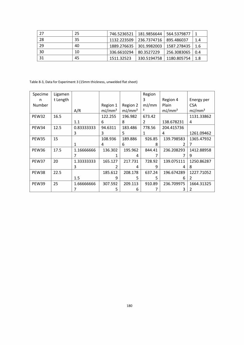
180

27 25 746.5236521 181.9856644 564.5379877 1

28 35 1132.223509 236.7374716 895.486037 1.4

29 40 1889.276635 301.9982003 1587.278435 1.6

30 10 336.6610294 80.3527229 256.3083065 0.4

31 45 1511.32523 330.5194758 1180.805754 1.8

Table 8-3, Data for Experiment 3 (15mm thickness, unwelded flat sheet)

Specimen

Number

Ligament Length

A/R Region 1 mJ/mm²

Region 2 mJ/mm²

Region3 mJ/mm²

Region 4 Plain mJ/mm²

Energy per CSA mJ/mm²

PEW32 16.5 1.1

122.2556

196.9828

673.422 138.678231

1131.338624

PEW34 12.5 0.833333333

94.63113

183.4865

778.561

204.4157364 1261.09462

PEW35 15 1

108.9364

189.8866

926.858

139.7985832

1365.479327

PEW36 17.5 1.166666667

136.3021

195.9624

844.417

236.2082937

1412.889589

PEW37 20 1.333333333

165.1272

217.7314

728.929

139.0751114

1250.862878

PEW38 22.5 1.5

185.6129

208.1785

637.245

196.6742896

1227.710522

PEW39 25 1.666666667

307.5925

209.1136

910.897

236.7099753

1664.313252

181

Part B (Chapter 4)

Table 8-4, Data for DOE analysis (15mm flat sheet specimen)

std The width of waisted section mm

The radius of the waisted section mm

The diameter of loading

holes mm

The distance between loading holes mm

Width of Specimen

mm

Energy to Break

(J/mm2)

Region3 (J/mm2)

Elongation in Pin(mm)

PEW101 14.9 5.1 15.2 80 45.2 809.1961 364.3367 0.13

PEW102 24.9 5.1 15.2 80 45.2 1080.742 259.7089 1.24

PEW103 14.9 10.15 15.2 80 45.2 1132.874 616.336 0.12

PEW104 24.9 10.15 15.2 80 45.2 1834.252 1068.009 1

PEW105 14.9 5.1 15.2 80 65.2 835.1929 431.7355 0.12

PEW106 24.9 5.1 15.2 80 65.2 942.9599 258.1319 0.8

PEW107 14.9 10.15 15.2 80 65.2 1509.592 1013.874 0.12

PEW108 24.9 10.15 15.2 80 65.2 1304.365 648.2134 0.76

PEW109 14.9 5.1 25.2 80 55.2 688.7907 250.0623 1.2

PEW110 24.9 5.1 25.2 80 55.2 484.2177 376.8149 0.2

PEW111 14.9 10.15 25.2 80 55.2 1264.639 689.5782 0.2

PEW112 24.9 10.15 25.2 80 55.2 1757.6 919.177 1.2

PEW113 14.9 5.1 25.2 80 75.2 910.1076 486.4859 0.21

PEW114 24.9 5.1 25.2 80 75.2 1164.935 498.2933 0.7

182

PEW115 14.9 10.15 25.2 80 75.2 1649.092 1216.461 0.2

PEW116 24.9 10.15 25.2 80 75.2 986.8058 694.4145 0.5

PEW117 14.9 5.1 15.2 100 45.2 822.3246 378.4455 0.1

PEW118 24.9 5.1 15.2 100 45.2 1178.127 387.454 0.35

PEW119 14.9 10.15 15.2 100 45.2 1334.236 864.1671 0.15

PEW120 24.9 10.15 15.2 100 45.2 1999.388 1199.178 1.2

PEW121 14.9 5.1 15.2 100 65.2 1129.612 685.9159 0

PEW122 24.9 5.1 15.2 100 65.2 1032.216 384.0297 0.9

PEW123 14.9 10.15 15.2 100 65.2 2054.445 1649.253 0.2

PEW124 24.9 10.15 15.2 100 65.2 2526.694 1969.593 0.85

PEW125 14.9 5.1 25.2 100 55.2 1121.507 696.5928 0

PEW126 24.9 5.1 25.2 100 55.2 1388.922 708.0142 0.37

PEW127 14.9 10.15 25.2 100 55.2 2482.264 2121.505 0

PEW128 24.9 10.15 25.2 100 55.2 2703.693 2093.886 0.9

PEW129 14.9 5.1 25.2 100 75.2 1111.588 727.3299 0.2

PEW130 24.9 5.1 25.2 100 75.2 1104.976 487.3565 0.5

PEW131 14.9 10.15 25.2 100 75.2 1991.228 1567.873 0.6

PEW132 24.9 10.15 25.2 100 75.2 1645.587 933.4105 0.2

PEW133 8 7.65 20.2 90 60.2 1391.585 1112.596 0.15

PEW134 30.2 7.65 20.2 90 60.2 1252.616 771.1275 1.35

PEW135 20.2 3 20.2 90 60.2 752.8557 269.7414 0.2

PEW136 20.2 13.5 20.2 90 60.2 2757.398 2259.556 0.4

PEW137 20.2 7.65 20.2 90 36.2 1012.117 647.7364 fail

PEW138 20.2 7.65 20.2 90 84.2 1553.965 967.6948 0.35

PEW139 20.2 7.65 8 90 48 0 0 0

PEW140 20.2 7.65 32 90 72 0 0 0

183

PEW141 20.2 7.65 20.2 66 60.2 2034.212 1529.164

PEW142 20.2 7.65 20.2 114 60.2 1886.057 1327.891 0.3

PEW143 20.2 7.65 20.2 90 60.2 1636.997 1065.347 0.35

PEW144 20.2 7.65 20.2 90 60.2 1669.388 1138.499 0

PEW145 20.2 7.65 20.2 90 60.2 1803.916 1317.454 0.35

PEW146 20.2 7.65 20.2 90 60.2 1729.729 1194.575 0.6

PEW147 20.2 7.65 20.2 90 60.2 1733.368 1188.844 0

PEW148 20.2 7.65 20.2 90 60.2 1713.618 1230.86 0.38

PEW149 20.2 7.65 20.2 90 60.2 1883.536 1393.809 0

PEW150 20.2 7.65 20.2 90 60.2 1486.788 938.9248 0.32

184

Table 8-5, ANOVA results for total energy response

Source SS DF MS F p-value

Model 1.043E+007 12 8.694E+005 11.51 < 0.0001

A-Width of Waisted Section 71422.35 1 71422.35 0.95 0.3377

B-Radius of the Waisted Section 6.727E+006 1 6.727E+006 89.07 < 0.0001

C-Diameter of Loading Holes 51454.19 1 51454.19 0.68 0.4149

D-Distance between Loading Holes 9.867E+005 1 9.867E+005 13.07 0.0010

E-Width of Specimen 865.66 1 865.66 0.011 0.9154

AE 4.752E+005 1 4.752E+005 6.29 0.0171

BD 3.410E+005 1 3.410E+005 4.52 0.0409

CD 1.270E+005 1 1.270E+005 1.68 0.2035

A2 2.005E+005 1 2.005E+005 2.66 0.1124

C2 4.690E+005 1 4.690E+005 6.21 0.0177

D2 1.086E+005 1 1.086E+005 1.44 0.2388

185

E2 1.509E+005 1 1.509E+005 2.00 0.1665

Residual 2.568E+006 34 75519.09 N/A N/A

Lack of Fit 2.471E+006 27 91519.54 6.63 0.0075

Pure Error 96621.43 7 13803.06 N/A N/A

Total 1.300E+007 46 N/A N/A N/A

Table 8-6, ANOVA results for Region 3 energy

ANOVA for Response Surface Reduced Quadratic model

Analysis of variance table [Partial sum of squares - Type III]

Source Sum of Square df Mean Square F Value p-value Prob >

F

Model 1.014E+007 11 9.221E+005 13.14 < 0.0001

A-Width of Waisted Section 74658.54 1 74658.54 1.06 0.3094

B-Radius of the Waisted Section 6.322E+006 1 6.322E+006 90.07 < 0.0001

186

C-Diameter of Loading Holes 1.472E+005 1 1.472E+005 2.10 0.1565

D-Distance between Loading

Holes

9.078E+005 1 9.078E+005 12.93 0.0010

E-Width of Specimen 35187.82 1 35187.82 0.50 0.4836

AE 3.106E+005 1 3.106E+005 4.43 0.0427

BD 4.953E+005 1 4.953E+005 7.06 0.0118

A2 1.003E+005 1 1.003E+005 1.43 0.2400

C2 5.601E+005 1 5.601E+005 7.98 0.0078

D2 94239.13 1 94239.13 1.34 0.2544

E2 3.130E+005 1 3.130E+005 4.46 0.0419

Residual 2.456E+006 35 70182.05 N/A N/A

Lack of Fit 2.316E+006 28 82714.35 4.12 0.0295

Pure Error 1.404E+005 7 20052.85 N/A N/A

Cor Total 1.260E+007 46 N/A N/A N/A

187

Table 8-7, ANOVA results for elongation in loading pin holes

ANOVA for Response Surface Linear model

Analysis of variance table [Partial sum of squares - Type III]

Source Sum of Squares df Mean Square F Value p-value Prob >

F

Model 4.56 5 0.91 10.62 < 0.0001

A-Width of

Waisted Section

3.69 1 3.69 43.02 < 0.0001

B-Radius of the

Waisted Section

9.220E-004 1 9.220E-004 0.011 0.9180

C-Diameter of

Loading Holes

0.10 1 0.10 1.21 0.2787

D-Distance

between

Loading Holes

0.11 1 0.11 1.32 0.2571

E-Width of

Specimen

0.36 1 0.36 4.20 0.0469

188

Residual 3.52 41 0.086 N/A N/A

Lack of Fit 3.24 34 0.095 2.35 0.1207

Pure Error 0.28 7 0.041 N/A N/A

Cor Total 8.08 46 N/A N/A N/A

Part C (Chapter 5)

Table 8-8, Constants used in constitutive equation

189

Figure 8-1, Tensile test engineering design for DIC purpose

Figure 8-2, Initial increment and mesh for PEW36 specimen for FEA result Figure 5-3

190

Figure 8-3, Mesh configuration for the wasited area of specimen PEW36 for FEA result Figure 5-3

Figure 8-4, Increment 7 for PEW36 specimen for FEA result in Figure 5-3

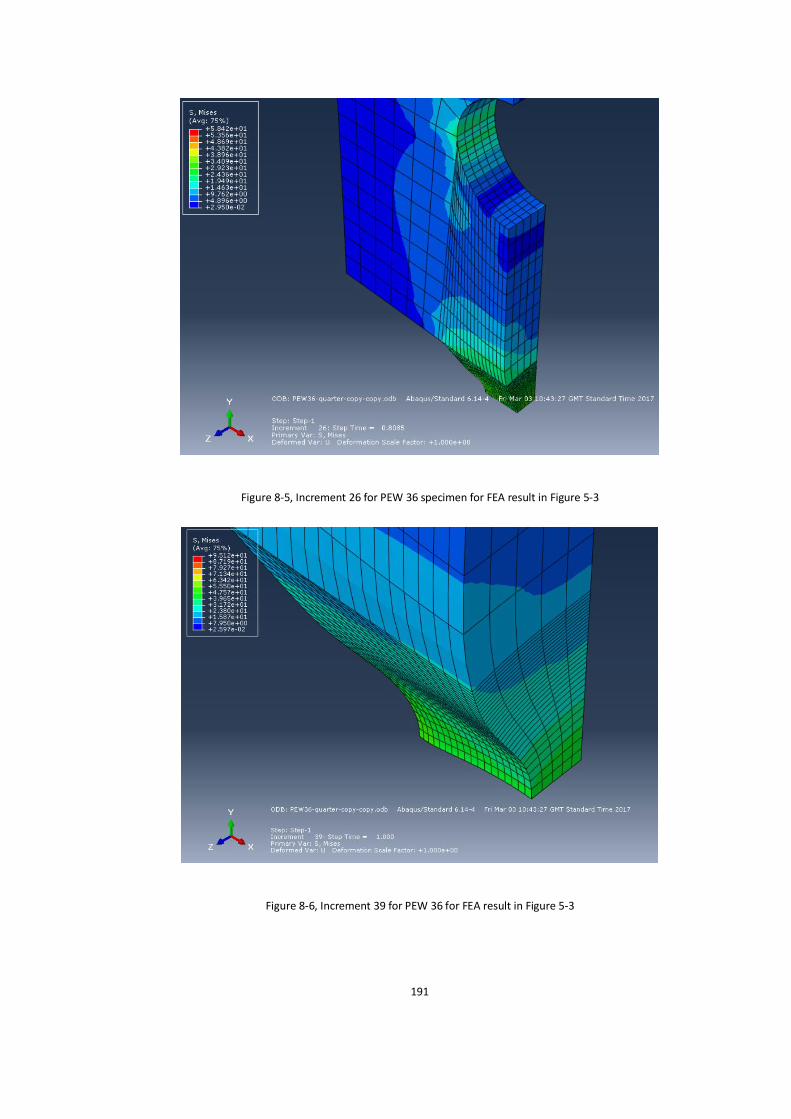
191

Figure 8-5, Increment 26 for PEW 36 specimen for FEA result in Figure 5-3

Figure 8-6, Increment 39 for PEW 36 for FEA result in Figure 5-3

192

Part D (Chapter 6)

Table 8-9, data for 140mm OD pipes

Specimen No Parent/Weld Geometry Position Pipe size Pipe/weld no

PEB149 Parent 12814-7 2 140SDR11 140P01

PEB150 Parent 12814-7 8 140SDR11 140P01

PEB151 Parent Modified 4 140SDR11 140P01


PEB153 Parent 12814-7 2 140SDR11 140P02

PEB154 Parent 12814-7 8 140SDR11 140P02



PEB157 Parent 12814-7 2 140SDR11 140P03

PEB158 Parent 12814-7 8 140SDR11 140P03



PEB161 Weld 12814-7 2 140SDR11 140W01

PEB162 Weld Modified 10 140SDR11 140W01

PEB163 Weld 12814-7 8 140SDR11 140W01


PEB165 Weld 12814-7 2 140SDR11 140W02


PEB167 Weld 12814-7 8 140SDR11 140W02


PEB169 Weld 12814-7 2 140SDR11 140W03


PEB171 Weld 12814-7 8 140SDR11 140W04

193


Specimen No

Parent/Weld Geometry Position Pipe size Pipe/Weld no

PEB173 Weld-No Bead 12814-7 2 140SDR11 140W01-B


PEB175 Weld-No Bead Modified-1

4 140SDR11 140W01-B

PEB176 Weld-No Bead Modified-1

10 140SDR11 140W01-B



PEB179 Weld-No bead

Modified-1

4 140SDR11 140W02-B

PEB180 Weld-No bead Modified-1

10 140SDR11 140W02-B

Table 8-10, Data for 160mm OD pipe

Specimen No Parent/Weld Geometry Position Pipe size Pipe/weld no

PEB101 Parent 12814-7 2 160SDR11 160P05

PEB102 Parent 12814-7 8 160SDR11 160P05



PEB105 Parent 12814-7 2 160SDR11 160P06

PEB106 Parent 12814-7 8 160SDR11 160P06



194

PEB109 Parent 12814-7 2 160SDR11 160P07

PEB110 Parent 12814-7 8 160SDR11 160P07



PEB113 Weld 12814-7 2 160SDR11 160W05


PEB115 Weld 12814-7 8 160SDR11 160W05


PEB117 Weld 12814-7 2 160SDR11 160W06


PEB119 Weld 12814-7 8 160SDR11 160W06


PEB121 Weld 12814-7 2 160SDR11 160W07

PEB122 Weld modified 10 160SDR11 160W07

PEB123 Weld 12814-7 8 160SDR11 160W07

PEB124 Weld modified 4 160SDR11 160W07


Specimen No

Parent/Weld Geometry Position Pipe size Pipe/weld no

PEB125 Parent 12814-7 12 250SDR17 250P013

PEB126 Parent 12814-7 4 250SDR17 250P013

PEB127 Parent 12814-7 8 250SDR17 250P013




195

PEB131 Parent 12814-7 12 250SDR17 250P014

PEB132 Parent 12814-7 4 250SDR17 250P014

PEB133 Parent 12814-7 8 250SDR17 250P014




PEB137 Weld 12814-7 12 250SDR17 250W013

PEB138 Weld 12814-7 4 250SDR17 250W013

PEB139 Weld 12814-7 8 250SDR17 250W013




PEB143 Weld 12814-7 12 250SDR17 250W014

PEB144 Weld 12814-7 4 250SDR17 250W014

PEB145 Weld 12814-7 8 250SDR17 250W014





PEB181 Parent 12814-7 1 280SDR11 280P15

PEB182 Parent 12714-7 4 280SDR11 280P15

PEB183 Parent 12814-7 7 280SDR11 280P15

PEB184 Parent 12814-7 10 280SDR11 280P15

PEB185 Parent Modified-3 3 280SDR11 280P15



196


PEB189 Welded 12814-7 1 280SDR11 280W15

PEB190 Welded 12814-7 4 280SDR11 280W15

PEB191 Welded 12814-7 7 280SDR11 280W15

PEB192 Welded 12814-7 10 280SDR11 280W15

PEB193 Welded Modified-3 3 280SDR11 280W15



PEB196 welded Modified-3 11 280SDR11 280W15


PEB197 Parent 12814-7 12 500SDR11 500P19

PEB198 Parent 12814-7 2 500SDR11 500P19

PEB199 Parent 12814-7 5 500SDR11 500P19

PEB200 Parent 12814-7 8 500SDR11 500P19

PEB201 Parent 12814-7 10 500SDR11 500P19

PEB202T Parent-Cut/2 Modified 1 500SDR11 500P19

PEB202B Parent-Cut/2 Modified 1 500SDR11 500P19









PEB206 Weld 12814-7 12 500SDR11 500W19

PEB207 Weld 12814-7 2 500SDR11 500W19

197

PEB208 Weld 12814-7 5 500SDR11 500W19

PEB209 Weld 12814-7 8 500SDR11 500W19

PEB210 Weld 12814-7 10 500SDR11 500W19

PEB211T Weld-cut/2 Modified 1 500SDR11 500W19

PEB211B Weld-cut/2 Modified 1 500SDR11 500W19










Specimen No

Parent/Weld Geometry Position Pipe size Pipe/weld no

PEB216 Parent 12814-7 12 630SDR11 630P21

PEB217 Parent 12814-7 2 630SDr11 630P21

PEB218 Parent 12814-7 5 630SDR11 630P21

PEB219 Parent 12814-7 8 630SDR11 630P21

PEB220 Parent 12814-7 10 630SDR11 630P21








198




PEB226 Weld 12814-7 12 630SDR11 630W21

PEB227 Weld 12814-7 2 630SDR11 630W21

PEB228 Weld 12814-7 5 630SDR11 630W21

PEB229 Weld 12814-7 8 630SDR11 630W21

PEB230 Weld 12814-7 10 630SDR11 630W21











199

Table 8-15, Data for all the weldings in this research

OD SDR Thickness No of Welds

Temp(⁰C) Heating up time(s)

Changeover time (S)

Cooling Time (min)

Weld No Welding Machine

Pressure(N/mm2)

140 11 12.7 2 211 127 8 to 10 16 to 24 140W01-02 BF315 0.15

140 11 12.7 2 211 127 8 to 10 16 to 24 140W03-04 BF315 0.15

160 11 14.5 2 209 145 8 to 10 16 to 24 160W05-06 BF315 0.15

160 11 14.5 2 209 145 8 to 10 16 to 24 160W07-08 BF315 0.15

200 11 18.2 2 206 182 8 to 10 16 to 24 200W09-10 BF315 0.15

200 11 18.2 2 206 182 8 to 10 16 to 24 200W11-12 BF315 0.15

250 17 14.7 1 209 147 8 to 10 16 to 24 250W13 BF315 0.15

250 17 14.7 1 209 147 8 to 10 16 to 24 250W14 BF315 0.15

280 11 25.5 1 202 255 10 to 12 24 to 32 280W15 BF315 0.15

280 11 25.5 1 202 255 10 to 12 24 to 32 280W16 BF315 0.15

500 11 45.5 1 200 455 16 to 20 45 to 60 500W19 Mc1236 0.15

500 11 45.5 1 200 455 16 to 20 46 to 60 500W20 Mc1236 0.15

630 11 57.3 1 200 573 20 to 25 60 to 80 630W21 Mc1236 0.15

630 11 57.3 1 200 573 20 to 25 60 to 80 630W22 Mc1236 0.15

OPTIMISATION OF WAISTED TENSILE TEST SPECIMEN …

Documents

Transcript of OPTIMISATION OF WAISTED TENSILE TEST SPECIMEN …