Optimisation of Thickener Performance: Incorporation of ...

Optimisation of Thickener Performance:

Incorporation of Shear Effects

by

Adam Anthony Holden Crust

B.E.Chem (Hons.)

Submitted in total fulfilment of the requirements for the degree of

Doctor of Philosophy

March 2017

Particulate Fluids Processing Centre

Department of Chemical Engineering

The University of Melbourne

Victoria, 3010, Australia

Produced on archival quality paper

ORCID iD: 0000-0003-0693-7788

“All models are approximations. Essentially, all models are wrong, but some are useful.

However, the approximate nature of the model must always be borne in mind.”

George E.P. Box

i

ABSTRACT

Dewatering processes such as sedimentation and consolidation of colloidal suspensions are

important to a wide range of industries, including waste water and mining. Within the

mining industry, massive quantities of tailings comprising mineral suspensions are processed

daily. The ability to effectively dewater tailings plays a major role in the successful operation

of the process. Modern dewatering theory developed by Buscall and White (1987) can

predict the dewatering behaviour of such suspensions. Combining modern dewatering theory

with a phenomenological model can be utilised in the design, operation and understanding of

a dewatering process. A lab scale batch settling test can be accurately predicted through the

combination of modern dewatering theory and developed phenomenological models. For a

mineral suspension settling within a laboratory batch settling test, the combination of modern

dewatering theory and phenomenological model can accurately predict the result of the

settling test. However, using the same approach, the ability to accurately predict the full

scale performance of gravity thickeners (Usher and Scales 2005, Usher et al. 2009, Zhang et

al. 2013, Grassia et al. 2014) eludes. Instead, current full scale gravity thickener models

result in an under estimation of thickener solids flux by a factor up 100 (Usher 2002).

Shear effects, introduced by raking within a thickener for example, are known to affect the

settling of suspensions; however, these have not been completely accounted for within

current phenomenological models. Shear alters the structure of a flocculated aggregate and

subsequently alters the dewatering behaviour of the overall suspension. This effect, known

as aggregate densification, can be attributed to the enhancement in dewatering observed when

a suspension experiences shear. Aggregate densification theory has previously been partially

included into thickener models (Usher et al. 2009, Zhang et al. 2013, Grassia et al. 2014);

however these models assume time independent densification and do not account for the

dynamic nature of the process. The dependencies on densification parameters have not been

critically studied.

Abstract

ii

This thesis investigates the role of shear effects on suspension dewatering. The key aim of

this research is to quantify the effect of shear on dewatering and in particular, the

enhancement of dewatering in a thickener induced through shear. The research objective is

to develop a process, in which simple batch settling tests can be performed, the results

analysed and utilised to predict the full scale thickener performance that correctly takes

dynamic shear effects into account.

Aggregate densification theory was applied to sheared laboratory batch settling scenarios to

quantify the effect of shear on material property characterisation. Sheared laboratory batch

settling tests were performed using a polymer flocculated calcite as a representative mineral

suspension and further analysed using novel analysis methods based on modifications to

current techniques such as predictive modelling and densification analysis developed by van

Deventer (2012). Batch settling tests were performed to investigate the relationship between

aggregate densification parameters and both network stress and the magnitude of shear.

Manipulating the shear magnitude showed no significant trend in the extent of densification

however trends were observed in the rate of densification. The rate of aggregate

densification increased with shear up until a critical shear value. Above this critical shear

value, the rate of densification was observed to be constant. It is believed that this critical

shear value corresponds to the minimum requirement for particles to collide such that below

this value, there is insignificant kinetic energy to cause any noteworthy deformation to the

aggregates. The effect of network strength on aggregate densification parameters was also

investigated. It was observed that a flocculated suspension with sufficiently high solids

concentration such that the aggregates interact and become networked, densify a further 5%

compared to shearing un-networked aggregates. In terms of thickener performance, raking

the networked solids resulted in an order of magnitude increase in thickener throughput.

Raking within a thickener is currently performed at the base of the thickener in order to aid

transport of the suspension. This increase in thickener throughput due to raking the

networked suspension is therefore already implemented however unaccounted for within

current thickener models. The implementation of these findings into thickener models has

the potential to account for the current underestimation.

Abstract

iii

To completely exploit the phenomenon of aggregate densification, the results of the work

suggest that the shear within the system needs to be at or above a critical value and that a

network bed must be present, maintained, and raked.

Current one-dimensional (pseudo two dimensional) steady state thickener models were

modified so as to account for the time dependent nature of aggregate densification. This

exercise involved combining the theories of aggregate densification; sedimentation and

suspension bed consolidation. The model uses material dewatering properties obtained from

laboratory batch settling tests and thickener operational parameters as inputs to produce

steady state solids flux predictions for a range of underflow solids concentrations. Modelling

scenarios involved manipulating thickener operational and aggregate densification

parameters. The results indicate that an order of magnitude increase in thickener

performance can be achieved when the shear rate is above the critical value determined

during sheared laboratory batch settling tests. Additionally, model applications to real

systems have been discussed and methods of utilisation to achieve process optimisation have

been demonstrated.

As a result of this experimental and modelling work, a new method for full scale thickener

modelling from simple laboratory batch settling tests has been developed. This method

incorporates the rate dependence of aggregate densification and hence provides increased

accuracy in the estimation of thickener performance compared to previous models. It is

important to note that this newly developed model has a few assumptions and limitations.

Assumptions and limitations include line settling, negligible wall effects, all aggregates are

equal, no solids exit the overflow, steady state operation, straight walled, equal distribution of

shear and no aggregate breakage. Although some assumptions are inherent to the model

being one dimensional it is suggested that further work goes into addressing such issues as

particle and aggregate size polydispersity and aggregate breakage in order to further increase

the accuracy of the model. Additionally, the development of a transient model in which shear

history is included is recommended.

v

DECLARATION

This is to certify that:

i. The thesis comprises only my original work towards the PhD

ii. Due acknowledgement has been made in the text to all other materials used,

iii. The thesis is less than 100,000 words in length, exclusive of tables, maps,

bibliographies and appendices

Adam Anthony Holden Crust

vii

ACKNOWLEDGEMENTS

First and foremost I would like to thank my supervisors, Prof. Peter Scales and Dr. Shane

Usher. This thesis would not be possible without their guidance and support. It was an

honour being able to work with true professionals who are amongst the greatest in their

corresponding fields. I would like to thank Peter, for continually reminding me of the goals

and aims of this project and keeping my on the path to provide truly useful results. Your

encouragement and insightful ideas over the years kept me going. I genuinely appreciate the

effort and time you spent guiding me to be the best I can.

Massive gratitude goes to Shane. Your door was always open for me to discuss any issues I

had, whether it was a gap in my understanding or troubles with modelling. You were always

able help, despite our discussions often leading towards more questions than answers. Your

constant ideas and new directions always kept me busy. Without your support and assistance

a lot of this thesis would not exist. To ensure I was writing and not stuck on anything, you

provided daily check-ups and discussions over the last month, which are unequivocally

appreciated. Without your assistance, this thesis would not have materialised in time.

I would like to acknowledge and thank all that contributed to the research presented within

this thesis. Firstly, to all the research project students over the years; James, Justin, Xun,

Rizal, and Almir, thank you for your assistance with performing experiments. Because of

your efforts, more batch settling experiments were able to be performed. I would also like to

thank Adrian Knight; you were always available for assistance with anything lab related,

which most often included trying to find “borrowed” equipment. To Dr. Stefan Berres, I

appreciate the knowledge and expertise you provided leading to the development and

application of a transient batch settling implicit scheme. To Prof. Paul Grassia, my

understanding of thickener modelling was significantly increased through the meetings and

discussions we had.

Acknowledgements

viii

This research was conducted as part of the AMIRA P266G: Improving Thickener

Technology project. I would like to acknowledge the industry sponsors of this project. I

would particularly like to thank all at CSIRO involved with this project especially Dr. Phillip

Fawell for his management of the project and his thorough and invaluable critique and

proofing of every project report and presentation.

As with all research funding is required, hence I would like to acknowledge the Australian

Postgraduate Award (APA) for my PhD scholarship and the AMIRA P266G project for

additional funding and support from the Particulate Fluids Processing Centre (PFPC), a

Special Research Centre of the Australian Research Council (ARC).

To everyone within the office over the years; Sam Skinner, Tiara Kusuma, Emma Brisson,

Eric Hoefgen, Sui So, Dr. Catherine Sutton, Hui-En Teo, Dr. Rudolf Spehar, Edward Ross,

Dr. Erin Spiden, thankyou for creating a vibrant, enthusiastic working environment.

Overcoming the commute and getting myself into the office every day was made easier,

knowing I would be walking into a friendly, supportive office.

I would like to thank my parents, without your support, hard work and discipline over the

years; I wouldn’t be the person I am today. Not only did you provide me with the

opportunities that I have in life, but you always supported and loved me. Your hard working

attitudes have encouraged me through my educational journey. A special gratitude goes to

Dad, you motivated me to pursue engineering as you did, and I have always looked up to you

as a role model and an inspiration. To my siblings, Angus, Madeline and Phoebe, we have all

grown to be different, free-spirited thinkers, however your support and interest in what I was

doing never wavered.

Lastly, I would like to thank my beautiful wife, Kylie, for your practical and emotional

support as well as your love as I travelled across my PhD journey. Thank you for tolerating

and supporting me as I went through the ups and downs that is a PhD rollercoaster. You

always cheered me up whenever I was upset with how my research was going, and you also

always managed to bring me back to earth when I thought everything was going perfectly. I

am amazed at your patience, and unrelenting love for me. Kylie, for your continuous support

throughout this adventure, and for all adventures to come, I dedicate this thesis to you.

ix

KEYWORDS

aggregate densification, aggregate restructuring, batch settling modelling, batch settling tests,

compressive yield stress, dewaterability characterisation, dynamic densification, flocculated

suspension, gravity thickening, hindered settling function, permeability enhancement,

thickener modelling

xi

TABLE OF CONTENTS

Abstract i

Declaration v

Acknowledgements vii

Keywords ix

Table of Contents xi

Publications xxi

List of Figures xxiii

List of Tables xli

Nomenclature xliii

Chapter 1. Thesis Overview 1

1.1 Background 1

1.2 Gravity Thickening 4

1.3 Raking and Shear Forces 6

1.4 Motivation for this Work 7

1.5 Research Objective 8

1.6 Thesis Outline 9

TableofContents

xii

Chapter 2. Theory 11

2.1 Dewatering Mechanics 12

2.1.1 Sedimentation 13

2.1.2 Consolidation 16

2.2 Modern Dewatering Theory 17

2.3 Shear Rheology 21

2.3.1 Shear rheology characterisation 22

2.3.2 Shear rheology models 22

2.4 Dewatering Material Properties 23

2.4.1 Gel point 23

2.4.2 Compressibility 23

2.4.3 Permeability 25

2.4.4 Solids flux 28

2.4.5 Solids diffusivity 29

2.5 Dewatering Material Properties: Characterisation 30

2.5.1 Batch settling 30

2.5.2 Centrifugation 34

2.5.3 Pressure filtration 34

2.6 Aggregation 37

2.6.1 Colloidal forces 38

TableofContents

xiii

2.6.2 Aggregation mechanisms 45

2.6.3 Aggregate formation and structure 47

2.7 Aggregate Densification 48

2.7.1 Experimental observations of aggregate densification 50

2.7.2 Aggregate parameters 52

2.7.3 Material properties: Incorporating densification 54

2.7.4 Modified Kynch method: Predicting settling curves with aggregate densification

58

2.7.5 Aggregate densification characterisation 61

2.8 Modelling of Transient Batch Settling 62

2.8.1 Finite discretisation 63

2.8.2 Implicit scheme 66

2.8.3 Accounting for aggregate densification 68

2.9 Thickener Modelling 69

2.9.1 1D steady state thickener modelling 70

2.9.2 Sedimentation theory 71

2.9.3 Consolidation theory 76

2.9.4 Solids residence time 78

2.9.5 Entropy condition 79

TableofContents

xiv

Chapter 3. Thickener Modelling 81

3.1 Background Theory 81

3.2 Model Assumptions and limitations 82

3.3 Model Inputs 84

3.3.1 Material properties 84

3.3.2 Operating conditions 86

3.3.3 Solids flux boundaries 86

3.4 Sedimentation Theory 88

3.4.1 Thickener sedimentation limited solids flux, qs 88

3.4.2 Solids concentration profile, φ(z) 89

3.4.3 Feed concentration limitations 89


3.4.5 Overall sedimentation flux 91

3.5 Un-networked and Networked Bed 92

3.6 Compression Theory 93

3.7 Model Algorithm 96

3.7.1 Core algorithm 96

3.7.2 Standard steady state thickener algorithm 100

3.7.3 Sedimentation limited solids flux algorithm 101

3.7.4 Dilute zone algorithm 102

TableofContents

xv

3.7.5 Permeability zone algorithm 102

3.7.6 Compressibility algorithm 103

3.7.7 Alternative networked bed method 104

3.8 Outputs: Model Thickener Performance Prediction 104

3.8.1 Alternative algorithm for networked bed 107

3.8.2 Mode 1: Permeability and q0 limited 108

3.8.3 Mode 2: Permeability, q0 and tres limited 110

3.8.4 Mode 3: Permeability limited 113

3.8.5 Mode 4: Networked permeability and compression limited 114

3.8.6 Mode 5: Compression limited 115


3.9 Impact of Process Variables 120

3.9.1 Suspension bed height 121

3.9.2 Feed concentration 123

3.9.3 Rate of aggregate densification 127

3.9.4 Shear during sedimentation 129

3.9.5 Feed densification state 132

3.10 Conclusions 134

TableofContents

xvi

Chapter 4. Raked Batch Settling 137

4.1 Experimental Outline 138

4.1.1 Material preparation 138

4.1.2 Experimental apparatus 139

4.1.3 Shear distributions within the raking rig 141

4.1.4 Experimental conditions 144

4.2 Confirmation of Aggregate Densification 146

4.2.1 Experimental procedure 146

4.2.2 Results 148

4.2.3 Discussion and conclusions 148

4.3 Stationary Rake 149

4.3.1 Analysis 150

4.3.2 Results 150

4.4 Experimental Consistency 155

4.4.1 Analysis 155

4.4.2 Results 155

4.5 Standard Raked Settling 158

4.5.1 Expected trends 158

4.5.2 Analysis 160


TableofContents

xvii

4.5.4 Results: Base conditions 161

4.5.5 Results: Rake rotation rate 166

4.5.6 Results: Initial height 172

4.5.7 Results: Flocculant dosage 179

4.6 Shear during Sedimentation 182

4.6.1 Expected trends 182

4.6.2 Analysis 183


4.6.4 Results 185

4.7 Shear during Consolidation 187

4.7.1 Expected trend 188

4.7.2 Analysis 188


4.7.4 Results: Base conditions 190

4.7.5 Results: Rake rotation rate 194

4.7.6 Results: Initial height 198

4.8 Overall Discussion and Conclusions 201

4.8.1 Raking zones 201

TableofContents

xviii

Chapter 5. Full Scale Prediction from Lab Scale Characterisation 205

5.1 Material Characterisation 206

5.1.1 Compressibility 206

5.1.2 Permeability 207

5.1.3 equationequationShear rheology 208

5.2 Aggregate Densification Parameters 210

5.2.1 Extent of aggregate densification 210

5.2.2 Shear during sedimentation 210

5.2.3 Shear during consolidation 226

5.3 Summarised Thickener Model Inputs 227

5.3.1 Operational conditions 227

5.3.2 Material properties 227

5.4 Results: Solids Flux vs. Underflow Solids Concentration 227

5.5 Conclusion 231

Chapter 6. Model Applications 233

6.1 Changes in Material Properties 233

6.1.1 Flocculation 234

6.1.2 Feed densification state 235

6.1.3 Stimuli responsive polymers 238

TableofContents

xix

6.1.4 Aggregate densification 239

6.1.5 Aggregate breakage 240

6.2 Shear during Sedimentation 240

6.2.1 Mechanical shear during sedimentation 240

6.3 Shear during Compression 241

6.3.1 Solids concentration effect on densification parameters 242

6.3.2 Channelling 246

6.3.3 True effect of bed height 246

6.3.4 Underflow limitations: Rake torque 247

6.4 Process Optimisation 257

6.4.1 Feed concentration 258

6.4.2 Flocculant type and flocculation conditions 260

6.4.3 Bed height 261

6.4.4 Feed particle size 262


6.4.6 Rate of aggregate densification 263

Chapter 7. Conclusions 267

7.1 Conclusions and Major Outcomes 268

7.1.1 Incorporation of dynamic densification into thickener models 268

TableofContents

xx

7.1.2 Impact of process variables on thickener performance 269

7.1.3 Effect of shear rate on densification parameters 269

7.1.4 Effect of network stress on densification parameters 270

7.1.5 Effect of shear zone 271

7.1.6 Method for full scale prediction from lab scale tests 271

7.1.7 Densification due to sedimentation 271

7.1.8 Rake torque estimates 272

7.2 Further Work and Future Directions 272

7.2.1 Aggregate densification parameter dependencies 273

7.2.2 Model short comings 273

7.2.3 Actual thickener performance 274

7.2.4 Flocculant dose 274

7.2.5 Dimensionless analysis 274

7.3 Overview 275

References 277

xxi

PUBLICATIONS

A. H. Crust, P. J. Scales, S. P. Usher (2015). Shear induced densification of flocculated

aggregates – characterising the effects on rheology. APCChE 2015 Congress incorporating

Chemeca 2015. Melbourne, Australia.

P. J. Scales, S. P. Usher, A. H. Crust (2015). Thickener modelling - from laboratory

experiments to full-scale prediction of what comes out the bottom and how fast. Paste 2015:

Proceedings of the 18th International Seminar on Paste and Thickened Tailings. Cairns,

Australia, Australian Centre for Geomechanics.

P. Grassia, Y. Zhang, A. D. Martin, S. P. Usher, A. H. Crust and R. Spehar (2014). Effects of

Aggregate Densification upon Thickening of Kynchian Suspensions. Chemical Engineering

Science. 111: 56-72

xxiii

LIST OF FIGURES

Figure1.1: Schematicofatypicalgravitythickener.............................................................5

Figure1.2: Schematic of the proposed effect of shear on aggregates. (Usher et al. 2009)..7

Figure2.1: SettlingofflocculatedsuspensionfromCoeandClevenger(1916)showingthe

differentzonesinthickening.(A)clearliquidzone,(B)Initialconcentrationzone,(C)

transitionzone,(D)consolidationzone..........................................................................18

Figure2.2: Typicalcompressiveyieldstress,Py(φ),asafunctionofsolidsvolumefraction,

φ.(A)Linearcoordinatesand(B)Semi-logarithmiccoordinates(AdaptedfromUsher

(2002)). ..........................................................................................................................25

Figure2.3: Typicalhinderedsettlingfunctionplot,R(φ),asafunctionofsolidsvolume

concentration,φ.(A)Linearcoordinatesand(B)Semi-logarithmiccoordinates.

(AdaptedfromUsher(2002))..........................................................................................28

Figure2.4: Typicalsolidsfluxvs.solidsconcentrationforaflocculatedmineralslurry.

Graphproducedusingadensitydifference,Δρ=2200kgm-3,andequation2.34to

describethehinderedsettlingfunctionwithparametersvalues,ra=5x1012,rg=-0.05,rn

=5andrb=0...................................................................................................................29

Figure2.5: Pressurefiltrationrigfordeterminationofmaterialpropertiesathighsolid

concentrations(Usheretal.(2001))...............................................................................36

Figure2.6: Theelectricaldoublelayereffectonanegativelychargedparticle(A)ionic

distributionand(B)electricalsurfacepotentialasafunctionofdistancefromthe

particlesurface(AdaptationfromGreen(1997))...........................................................41

Figure2.7: Netinterparticleforce(FT)asafunctionofparticleseparation(H)(Adapted

fromThomasetal.(1999))..............................................................................................44

ListofFigures

xxiv

Figure2.8: (a)Netinter-particleforce(FT)vsseparationdistance(H)astheelectrical

doubleandnetattractiveforcesaredepleted.(Adaptedfrom(Lim2011))(b)Particle

chargesandassociatedinteractionwithotherparticlesfordifferentmagnitudesofnet

attractiveforce................................................................................................................45

Figure2.9: Aggregationofparticlesduetobridgingflocculationwithhighmolecular

weightpolymers..............................................................................................................46

Figure2.10: (Left)Scaledaggregatediametervs.time.(AdaptedfromvanDeventeret

al.(2011))(Right)Changeinaggregatediametervs.time.(Dagg∞=0.9andA=0.01s-1).

.......................................................................................................................54

Figure2.11: Typicalcompressiveyieldstresscurves,Py(φ,Dagg),atvariousextentsof

aggregatedensification.(Dagg=1,0.95,0.90,0.85)(Usheretal.2009).......................56

Figure2.12: (A)Variationinsettlingvelocitieswithsolidsvolumefractionwhereu1isthe

flowaroundtheaggregatesandu2istheflowthroughtheaggregates.Examplegivenis

forDagg=1(Usheretal.2009).(B)Typicalhinderedsettlingfunctionvs.solidsvolume

fractionatdifferentextentsofaggregatedensification(Usheretal.2009)..................58

Figure2.13: Scaledaggregatediameterasafunctionoftime,Dagg(t),asdescribedby

equation2.106usingparameters:A=0.01s-1,Dagg,∞=0.9,tstart=100sandtstop=300s.

.......................................................................................................................69

Figure2.14: Steadystatethickenerperformancepredictionsofsolidsflux,q,vs.

underflowsolidsconcentration,φu,forarangeofextentsofaggregatedensificationand

abedheightof1m.(UsherandScales2005,Usheretal.2009)...................................71

ListofFigures

xxv

Figure2.15: Solidsflux,q(ms-1)calculatedviamaterialbalance(equation2.108)ata

rangeofsolidsconcentration,φ(v/v),forapermeability-limitedthickenerwithout

densification.Typicalmineralsuspensionmaterialpropertiesandanoperating

underflowconcentration,φu,of0.1v/vwereused.Thelocalminima,q=3.5x10-5ms-1,

providesthemaximumoperatingsolidsflux,qop.Atqop,twopotentialsolids

concentrationsarepossible,φ1andφ2,whichrepresentthesolidsconcentrationprofile.

.......................................................................................................................73

Figure2.16: Examplesolidsconcentrationprofile,z(φ),forapermeabilitylimited

thickenerwithoutdensificationoperatingatanunderflowsolidsconcentrationand

solidsfluxofφu=0.1v/vandqop=3.5x10-5ms-1.Afeedandbedheightof5and1m

wereused.Solidsconcentrations,φ1andφ2,weredeterminedviaequation2.108

(illustratedinFigure2.15)...............................................................................................74

Figure2.17: Examplesolidsflux,q(ms-1)vs.solidsconcentration,φ(v/v),foragiven

underflowsolidsconcentration,φu(v/v)atvaryingextentsofdensification.Solving

equation2.81resultsinoperatingfluxesof3.8x10-5,5.6x10-5and9x10-5ms-1forDagg=

1,0.95and0.90respectively(shownbyhorizontaldashedlines).Notethatthisresult

assumestimeindependentmaterialproperties.............................................................75

Figure2.18: Exampleofasolidsconcentrationprofile,z(φ),forathickeneroperated

withinpermeabilitylimitationsatarangeofdensificationextents.Forthisexamplea

feedandbedheightof5and1mwereusedalongwithanunderflowconcentrationof

0.1v/v.Notethateachsolidsconcentrationprofileisatadifferentoperatingfluxand

thatthisresultassumestimeindependentmaterialproperties....................................76

ListofFigures

xxvi

Figure3.1: Undensified(Dagg=1)andfullydensified(Dagg=Dagg,∞=0.8)hinderedsettling

function,R(φ,t),andcompressiveyieldstressfunction,Py(φ,t),usedinthemodelcase

studytopredictthickenerthroughput,q,asafunctionofunderflowsolids

concentrations,φu.Thehinderedsettlingfunctionisgovernedbyequations2.34and

2.73withparametervaluesra=5x1012,rg=-0.05andrn=5.Thecompressiveyield

stressfunctionalformisgovernedbyequations2.24,2.64and2.66withparameter

valuesa0=0.9,b=0.002andk0=11..............................................................................85

Figure3.2: Undensified(Dagg=1)andfullydensified(Dagg=Dagg,∞=0.8)solidsflux,f(φ,t)

vs.solidsconcentration,φ,wheref(φ,t)=φ.u(φ,t)..........................................................86

Figure3.3: Steadystatethickenerperformancepredictionsintermsofsolidsflux,q,

versusunderflowsolidsvolumefraction,φu,fornodensification,Dagg=1,andfull

densification,Dagg=Dagg,∞=0.8.....................................................................................87

Figure3.4: Sedimentationlimitedsolidsfluxboundariesaccordingtothefeedlimited

solidsflux,q0,andsteadystatethickenerperformancepredictionsintermsofsolids

flux,q,versusunderflowsolidsvolumefraction,φu,fornodensification,Dagg=1,and

fulldensification,Dagg=Dagg,∞=0.8...............................................................................90

Figure3.5: Profileofsolidsconcentrationφandsolidsgelpointφgvs.heightzforthecase

ofsedimentationlimitedsettlingwhere(left)q=0.29tonnesm-2hr-1,φu=0.18v/v,A(z

>hb)=0,A(z≤hb)=10-4s-1andDagg∞=0.8 (right)q=0.29tonnesm-2hr-1,φu=0.30v/v,

A(z>hb)=0,A(z≤hb)=10-4s-1andDagg∞=0.8.Thehorizontaldashedlinesindicatethe

(uniform)bedandnetworkedheights,hb(2m)andhn(0and0.89m)..........................93

Figure3.6: Profileofsolidsconcentrationφandsolidsgelpointφgvs.heightzforthecase

ofcompressionlimitedsettlingwhere(left)q=0.17tonnesm-2hr-1,φu=0.30v/v,A(z>

hb)=0,A(z≤hb)=10-3s-1andDagg∞=0.8(right)q=0.07tonnesm-2hr-1,φu=0.32v/v,

A(z>hb)=0,A(z≤hb)=10-3s-1andDagg∞=0.8.Thehorizontaldashedlinesindicatethe

(un-networked)bedandnetworkedbedheights,hb(2m)andhn(0and1.85m).........96

ListofFigures

xxvii

Figure3.7: Blockflowdiagramofcorealgorithmusedtopredictsteadystatethickener

performanceintermsofsolidsfluxvs.underflowsolidsconcentrationaswellassolids

concentrationprofiles.....................................................................................................99

Figure3.8: Steadystate(straightwalled)thickenermodelpredictionofthesolidsfluxasa

functionofunderflowsolidsvolumefractionforA(z>hb)=0,A(z≤hb)=10-4s-1,Dagg,∞=

0.8,φ0=0.05v/v,hf=5mandhb=2m.Upperandlowersolidsfluxpredictions(Dagg=

1andDagg=Dagg,∞)arealsoshown...............................................................................106

Figure3.9: Steadystate(straightwalled)thickenermodelpredictionofthesolidsfluxasa

functionofunderflowsolidsvolumefractionforA(z>hb)=0,A(z≤hb)=10-4s-1,Dagg,∞=

0.8,φ0=0.05v/v,hf=5mandhb=2m.Thickenerpredictionshavebeenperformed

usingtwoalgorithms,onemorecomputationallydemandingthantheother.Upperand

lowersolidsfluxpredictions(Dagg=1andDagg=Dagg,∞)arealsoshown....................108

Figure3.10: Solidsflux,q(tonneshour-1m-2),vs.solidsconcentration,φ(v/v),and

correspondingsolidconcentrationprofile,φ(z)foranunderflowsolidsconcentrationof

0.06v/v,operatingunderfeedfluxlimitations.Aggregatedensificationparametersof

Dagg,∞=0.8,A(z>hb)=0andA(z≤hb)=10-4s-1..........................................................109

Figure3.11: Theprofileoftheheightinthethickenervs.thesolidsvolumefraction–for

comparatively‘small’underflowsolidsconcentrations,φu=0.06,0.07and0.08v/v,in

whichthethickenerisoperatedunderfeedfluxlimitationsandnobedisachievable.

AggregatedensificationparametersofDagg,∞=0.8,A(z>hb)=0andA(z≤hb)=10-4s-1...

.....................................................................................................................110


correspondingsolidconcentrationprofiles,φ(z)foranunderflowsolidsconcentrationof

0.10v/v,operatingunderfeedflux,q0,andsolidresidencetime,tres,limitations.


.....................................................................................................................111

ListofFigures

xxviii


comparatively‘small’underflowsolidsconcentrations,φu=0.10,0.12,0.14and0.16

v/v,inwhichthethickenerisoperatedunderfeedfluxandsolidresidencetime

limitations.Thespecifiedbedheightisunobtainableandsmallerbedsareachieved.


.....................................................................................................................112


correspondingsolidconcentrationprofile,φ(z)foranunderflowsolidsconcentrationof

0.18v/v,operatingunderpermeabilitylimitations.Aggregatedensificationparameters

ofDagg,∞=0.8,A(z>hb)=0andA(z≤hb)=10-4s-1.......................................................113


comparatively‘intermediate’underflowsolidsconcentrations,φu=0.17,0.18,0.19and

0.20v/v,inwhichthethickenerisoperatedunderpermeabilitylimitations.Aggregate

densificationparametersofDagg,∞=0.8,A(z>hb)=0andA(z≤hb)=10-4s-1.............114


comparatively‘intermediatetohigh’underflowsolidsconcentrations,φu=0.20,0.25

and0.30v/v,inwhichthesuspensionbedisoperatedunderbothpermeabilityand

compressibilitylimitations.AggregatedensificationparametersofDagg,∞=0.8,A(z>hb)

=0andA(z≤hb)=10-4s-1..............................................................................................115


comparatively‘high’underflowsolidsconcentrations,φu=0.31v/v,inwhichthe

thickenerisoperatedundercompressibilitylimitations.Aggregatedensification

parametersofDagg,∞=0.8,A(z>hb)=0andA(z≤hb)=10-4s-1....................................116

ListofFigures

xxix

Figure3.18: Solidsresidencetime,tres(hr),vs.underflowsolidsconcentration,φu(v/v),for

hf=5m,hb=2m,A(z>hb)=0,A(z≤hb)=10-4s-1,Dagg,∞=0.8andφ0=0.05aswellas

thepredictedsolidsresidencetimefortimein-dependentmaterialpropertieswithDagg

=1andDagg=Dagg,∞=0.8.Thedashedlinerepresentsthedilutezonewithbedheight<

hb,theopensquaresaresedimentationlimitedandclosedsquaresarecompression

limitedsolutionpoints..................................................................................................118

Figure3.19: Overallsolidsresidencetime,tres(hr),vs.underflowsolidsconcentration,φu

(v/v),forhf=5m,hb=2m,A(z>hb)=0,A(z≤hb)=10-4s-1,Dagg,∞=0.8andφ0=0.05as

wellasthepredictedsolidsresidencetimeineachzoneofthethickener..................120

Figure3.20: Steadystate(straightwalled)thickenermodelpredictionofthesolidsfluxas

afunctionofunderflowsolidsvolumefractionfordifferentbedheights,hb=1,2and4

m.AggregatedensificationandthickeneroperationparametersofA(z>hb)=0,A(z≤

hb)=10-4s-1,Dagg,∞=0.8andφ0=0.05v/vwereused.Upperandlowersolidsflux

predictions(Dagg=1andDagg=Dagg,∞)arealsoshown................................................122


hb=1,2and4m,A(z>hb)=0,A(z≤hb)=10-4s-1,Dagg,∞=0.8andφ0=0.05v/v........123


afunctionofunderflowsolidsvolumefractionfordifferentfeedconcentrations,φ0=

0.005,0.02,0.05and0.08v/v.Aggregatedensificationandthickeneroperation

parametersofA(z>hb)=0,A(z≤hb)=10-4s-1,Dagg,∞=0.8,hf=5mandhb=2mwere

used.Upperandlowersolidsfluxpredictions(Dagg=1andDagg=Dagg,∞)arealso

shown. .....................................................................................................................125


afunctionofunderflowsolidsvolumefractionfordifferentfeedconcentrations,φ0=

0.005,0.02,0.05and0.08v/v.Aggregatedensificationandthickeneroperation

parametersofA(z>hb)=0,A(z≤hb)=10-4s-1,Dagg,∞=0.8,hf=5mandhb=2mwere

used.Upperandlowersolidsfluxpredictions(Dagg=1andDagg=Dagg,∞)arealso

shown. .....................................................................................................................126

ListofFigures

xxx


hb=2m,A(z>hb)=0,A(z≤hb)=10-4s-1,Dagg,∞=0.8andφ0=0.005,0.02,0.05and

0.08v/v. .....................................................................................................................127


afunctionofunderflowsolidsvolumefractionforratesofaggregatedensification,A(z≤

hb)=10-5,10-4,10-3-1.Aggregatedensificationandthickeneroperationparametersof

Dagg,∞=0.8,A(z>hb)=0,hf=5m,hb=2mandφ0=0.05v/vwereused.Upperand

lowersolidsfluxpredictions(Dagg=1andDagg=Dagg,∞)arealsoshown.....................128


hb=2m,A(z>hb)=0,A(z≤hb)=10-4s-1,Dagg,∞=0.8andφ0=0.005,0.02,0.05and0.08

v/v.Dashedlinesrepresentfeedfluxlimitedscenarios,un-filledsquaresare

sedimentationlimited,andfilledsquaresarecompressionlimited.............................129

Figure3.27: Performanceenhancementfactor,PE,vs.underflowsolidsvolumefraction,

φu,forsteadystate(straightwalled)thickenermodelpredictionsquantifyingtheeffect

ofdensificationwithinthedilutezoneofthethickener...............................................131


afunctionofunderflowsolidsvolumefractionforarepresentativemineralslurryfor

differentfeeddensificationstates,Dagg,0=1and0.95.Aggregatedensificationand

thickeneroperationparametersofA(z>hb)=0,A(z≤hb)=10-4s-1,Dagg,∞=0.8,hf=5,hb

=5andφ0=0.05v/vwereused....................................................................................133

Figure3.29: Steadystate(straightwalled)thickenermodelpredictionofthesolids

residencetimeasafunctionofunderflowsolidsvolumefractionforarepresentative

mineralslurryfordifferentfeeddensificationstates,Dagg,0=1and0.95.Aggregate

densificationandthickeneroperationparametersofA(z>hb)=0,A(z≤hb)=10-4s-1,

Dagg,∞=0.8,hf=5,hb=5andφ0=0.05v/vwereused.................................................134

ListofFigures

xxxi

Figure4.1: (a)Variableheightcylinderswithdetachablesegments.(b)Cylindersegment

joints.(c)Rakingrigusedforshearedbatchsettlingexperiments.(d)Rakesusedto

impartshearontosettlingsuspension(vanDeventer,Usheretal.2011)....................140

Figure4.2: Chainandgearsystemusedwithintherakedbatchsettlingrigtoimpart

differentshearratestotheaggregatedsuspensions...................................................141

Figure4.3: ShearrheologiesofmaterialsusedwithinCFDsimulationstodeterminethe

relationbetweenshearrateandrakerotationratewithintherakedbatchsettling

apparatus.MaterialrheologyprofilesareapproximatedtoaHerschel-Bulkleyfluid

(DataobtainedfromSpehar(2014)).............................................................................142

Figure4.4: Averagemaximumshearrateasafunctionofrakerotationrateintheraked

batchsettlingrig(DataobtainedfromSpehar(2014)).................................................143

Figure4.5. ProjecteddiametersfoundusingPVMprobeforOmyacarb2(0.03v/v),

Omyacarb10(0.03v/v)andkaolin(0.025v/v,10-3MKNO3,pH8).Flocculation

performedinapipereactorat40gt-1usingAN934SH.Rakingwasperformedfor1hour

atω=0.85rpm.Dotsindicateoutlierswithinthedata...............................................148

Figure4.6: Transientinterfacesettlingheightforthesettlingofflocculated(40gt-1

AN934SH)calcite(Omyacarb2,φ0=0.03v/v)withandwithoutastationaryrake......151

Figure4.7: CompressiveYieldStress,Py(φ)asafunctionofsolidsconcentration,φ,for

flocculated(AN934SHat40gt-1)calcite(Omyacarb2,φ0=0.03v/v)determinedvia

batchsettlingtestswithandwithoutastationaryrakepresent..................................152

Figure4.8: Hinderedsettling,R(φ)asafunctionofsolidsconcentration,φ,forflocculated

(AN934SHat40gt-1)calcite(Omyacarb2,φ0=0.03v/v)determinedviabatchsettling

tests,withandwithoutastationaryrakepresent........................................................153

Figure4.9: Hinderedsettlingfunction,R(φ)asafunctionofsolidsvolumefractionfora

rangeofun-shearedbatchsettlingtestsofflocculated(AN934SHat40gt-1)calcite

(Omyacarb2,φ0=0.03v/v)withaninitialheightof0.3m..........................................156

ListofFigures

xxxii

Figure4.10: Compressiveyieldstress,Py(φ),asafunctionofsolidsvolumefractionfora

rangeofun-shearedbatchsettlingtestsofflocculated(AN934SHat40gt-1)calcite


Figure4.11: Sedimentinterfaceheight,h(t)forsheared(ω=0.21rpm)andun-sheared

batchsettlingtestsofflocculated(AN934SHat40gt-1)calcite(Omyacarb2,φ0=0.03

v/v)withaninitialheightof0.3m...............................................................................162

Figure4.12: Compressiveyieldstress,Py(φ)asafunctionofsolidsvolumefractionforun-

densified(Dagg=1)anddensified(Dagg=Dagg,∞=0.88)batchsettlingtestsofflocculated

(AN934SHat40gt-1)calcite(Omyacarb2,φ0=0.03v/v)withaninitialheightof0.3m...

.....................................................................................................................163

Figure4.13: Hinderedsettlingfunction,R(φ)asafunctionofsolidsvolumefractionforun-

densified(Dagg=1)anddensified(Dagg=Dagg,∞=0.88)batchsettlingtestsofflocculated

(AN934SHat40gt-1)calcite(Omyacarb2,φ0=0.03v/v)withaninitialheightof0.3m...

.....................................................................................................................164

Figure4.14: Meanproportionalerrorintimeversusthedensificationrateparameter,A,

calculatedfortheoptimisationofthepredictedinterfaceheightagainstexperimental

dataforthesheared(ω=0.21rpm)settlingofflocculated(40gt-1AN934SH)calcite

(Omyacarb2,φ00.03v/v).............................................................................................165

Figure4.15: Predictedsedimentinterfaceheight,h(t),curvefitincorporatingaggregate

densificationusingtheoptimumvalueofA(0.00135s-1).Predictedandexperimental

datarepresentsbatchsettlingtestsofflocculated(AN934SHat40gt-1)calcite


Figure4.16: Normalisedsedimentinterfaceheight,H(t)forbatchsettlingtestsof

flocculated(AN934SHat40gt-1)calcite(Omyacarb2,φ0=0.03v/v)withaninitial

heightof0.3mandshearedatrotationrates,ω,of0,0.21,2.09,4.2and8.63rpm.

Dataatotherrotationrateswereomittedforclarity...................................................167

ListofFigures

xxxiii

Figure4.17: Extentofaggregatedensificationasafunctionofrotationrate,ω,for


settlingheightof0.3m.Theresultsarecombinedfromthreesetsofdata................168

Figure4.18: Aggregatedensificationrateparameter,A,(s-1),asafunctionofrake

rotationrate,ω,forflocculated(AN934SHat40gt-1)calcite(Omyacarb2,φ0=0.03v/v)

withaninitialsettlingheightof0.3m.Thedatawasextractedusingthemodified

Kynchmethodtooptimisepredictedsettlingcurves(vanDeventeretal.(2011))......170

Figure4.19: Sedimentinterfaceheight,h(t)forun-shearedbatchsettlingtestsof

flocculated(AN934SHat40gt-1)calcite(Omyacarb2,φ0=0.03v/v)withinitialheights

of0.26,0.6,0.9and1.2m............................................................................................174

Figure4.20: Hinderedsettlingfunction,R(φ),asafunctionofsolidsconcentration,φ(v/v),

forthesettlingofflocculated(40gt-1AN935SH)calcite(Omyacarb2atφ0=0.03v/v)at

variousinitialsettlingheights.Solidsconcentrationrangehasbeenrestrictedbetween

φ0=0.03v/vandthefanlimitsolidsconcentration,φfl=0.13v/v...............................175

Figure4.21: Compressiveyieldstress,Py(φ),asafunctionofsolidsconcentration,φ(v/v),

forthesettlingofflocculated(40gt-1AN935SH)calcite(Omyacarb2atφ0=0.03v/v)at

variousinitialsettlingheights.......................................................................................176

Figure4.22: Normalisedtransientinterfaceheight,H(t)forthesettlingforflocculated(40

gt-1)Omyacarb2(φ00.03v/v)un-shearedandsheared(ω = 0.21rpm)forinitialheights

of0.26and1.22m........................................................................................................178

Figure4.23: Normalisedtransientheight,H(t),forshearedandun-shearedsettlingtests

ofcalcite(Omyacarb2at0.03v/v)flocculatedwithAN934SHat0,40and80gt-1.The

shearedsettlingtestswererakedatarotationrateof0.2rpmuntildewatering

effectivelyceased(72hr)..............................................................................................180

ListofFigures

xxxiv

Figure4.24. TransientheightversustimeforrakedsettlingtestsofOmyacarb2at0.03

v/v,flocculatedwithAN934SHat40gt-1conductedatarotationrateof0.072rpmand

variousrakestoptimes,tstop=179,840and1300s.Filledsymbolsindicateraked

portionofthesettlingcurve.Initialheightsrangefrom0.25to0.28m......................186

Figure4.25: Sedimentinterfaceheight,H(t)forun-shearedandsheared(ω=0.21rpm)

batchsettlingtestsofflocculated(AN934SHat40gt-1)calcite(Omyacarb2,φ0=0.03

v/v)withaninitialheightof0.3m.Rakingwasperformedsolelywithinthenetworked

suspensionbycommencingrakingoncethemajorityofaggregateshadsettled(approx.

1hr) .....................................................................................................................191

Figure4.26: Compressiveyieldstress,Py(φ,Dagg)curvefitasafunctionofsolidsvolume

fractionforun-densified(Dagg=1)anddensified(Dagg=Dagg,∞=0.84)batchsettling

testsofflocculated(AN934SHat40gt-1)calcite(Omyacarb2,φ0=0.03v/v)withan

initialheightof0.3m....................................................................................................193

Figure4.27: Hinderedsettlingfunction,R(φ,Dagg)curvefitasafunctionofsolidsvolume

fractionforun-densified(Dagg=1)anddensified(Dagg=Dagg,∞=0.84)batchsettling

testsofflocculated(AN934SHat40gt-1)calcite(Omyacarb2,φ0=0.03v/v)withan

initialheightof0.3m....................................................................................................194

Figure4.28: Unshearedandsheared(ω=0.10,0.21and4.24rpm)batchsedimentation

dataforflocculatedOmyacarb2usingAN934SHat40gt-1.Rakingcommencedonce

themajorityofaggregateshadsettled(approx.1hr,T=1).........................................195

Figure4.29: Focusoftheunshearedandsheared(ω=0.10,0.21and4.24rpm)batch

sedimentationdataforflocculatedOmyacarb2usingAN934SHat40gt-1.Raking

commencedoncethemajorityofaggregateshadsettled(approx.1hr).....................196

Figure4.30: Finalscaledaggregatediameterasafunctionofrotationrateforsheared

settlingtestsofcalcite(Omyacarb2,φ0=0.03v/v)flocculatedwithAN934SHata

dosageof40gt-1.Shearwasperformedexclusivelyduringtheconsolidationregime.....

.....................................................................................................................198

ListofFigures

xxxv

Figure4.31: Averagebedsolidsconcentration,φf,aveforunshearedandnetworked

shearedsedimentationtestsofpolymerflocculatedOmyacarb2(40and80gt-1

AN934SH).Foraguidetoextentofdensification,linesofconstantDagg,∞areshown......

.....................................................................................................................199

Figure4.32: Finalscaledaggregateddiameter,Dagg,∞,forunshearedandnetworked

shearedsedimentationtestsofpolymerflocculatedOmyacarb2(40and80gt-1

AN934SH)......................................................................................................................200

Figure4.33: Scaledequilibriumaggregatediameterasafunctionofrakerotationrate,

Dagg,∞(ω),forvariousshearedsettlingexperimentsofflocculated(AN934SHat40gt-1)

calcite(Omyacarb2,φ0=0.03v/v)withaninitialsettlingheightof0.3m..................202

Figure4.34: Rateofdensification,A,(s-1),asafunctionofrakerotationratefor


settlingheightof0.3m.Thezoneinwhichshearwasimpartedishighlight.Additional

resultbyvanDeventer(2012)isalsoincluded.............................................................203

Figure5.1: Un-densifiedcompressiveyieldstressandhinderedsettlingfunctions,Py,0(φ)&

R0(φ),usedwithinthemodelcasestudy.Py,0(φ)andR0(φ)weredeterminedviafitting

equations2.24and2.34toexperimentaldataresultinginfittingparametervaluesofra

=6.37x1012,rg=-0.028,rn=4.14,a0=0.80,b=0.01,k0=5.52,φg,=0.188v/vandφcp,=

0.63v/v.........................................................................................................................208

Figure5.2: Herschel-Bulkleyparamters,K(φ)andn(φ)usedtodescribetheshearrheology

offlocculatedOmyacarb2.DatafromSpehar(2014)..................................................209

Figure5.3: Shearstress,τ,andviscosity,η,asafunctionofshearrate,γforflocculated

calcite(Omyacarb2)atvarioussolidsconcentrations,φ,givenbyequations2.21and

2.22.ShearrheologyhasbeenmodelledusingaHerschel-Bulkleyfitwithparameter’s,

K(φ)andn(φ)describedbyequation5.1and5.2.Anominalvalueof20hasbeenused

fortheratiobetweenthecompressiveandshearyieldstresses,α,forsolids

concentrationsof0.2and0.3v/v.................................................................................210

ListofFigures

xxxvi

Figure5.4: Flowregimedragcoefficientcorrectionfactor,χRep,asafunctionofparticle

ReynoldsnumbertoaccountforthedeviationinthedragcoefficientfromtheStokes

dragcoefficient.............................................................................................................216

Figure5.5: Ratioofperfectsliptonoslipdragcoefficients,χBC=CD,slip/CD,non-slip,asa

functionofsolidsvolumefraction,φ.Ratioscalculatedbasedondragcoefficientvalues

determinedbyDattaandDeo(2002)...........................................................................218

Figure5.6: (a)Shearstress,τ,asafunctionofrakerotationratedeterminedviaequation

5.21atsolidsconcentration,φ=φ0=0.03,φ=φfl=0.118andφ=φave=0.074v/v.(b)

Densificationrateparameter,A(s-1),asafunctionofrakerotationrate,ω,givenby

equation4.4anddeterminedfromshearedbatchsettlingtestsofflocculated(40gt-1

AN934SH)calcite(Omyacarb2,φ0=0.03v/v)..............................................................220

Figure5.7: Densificationrateparameter,A(s-1),asafunctionofshearstress,τ,basedon

CFDsimulationsandexperimentallyobservedtrends(equations5.21and4.4)..........221

Figure5.8: Particlesettlingvelocity,u,andReynoldsnumber,Rep,vs.solids

concentration,φ,foranundensified(Dagg=1)andfullydensified(Dagg=Dagg,∞=0.86)

calciteaggregate,ρsol=2710kgm-3anddagg,0=116µm,settlinginwater,ρliq=1000kg

m-3andη=0.001Pas...................................................................................................223

Figure5.9: (a)Aggregatedragcoefficient,CD,agg,asafunctionofsolidsvolumefraction

forthesedimentationofflocculatedcalcite(Omyacarb2,40gt-1AN934SH).Thedrag

coefficienthasbeencorrectedtoaccountforflowregimeandfullslipboundary

condition.(b)Averageandmaximumshearstress,τ0,onthesurfaceofanundensified

(Dagg=1)andfullydensified(Dagg=Dagg,∞=0.86)calciteaggregate,dagg,0=116µmand

ρsol=2710kgm-3,duetotheflowofwater,ρliq=1000kgm-3andη=0.001Pas,

aroundtheaggregate.Shearstresshasbeenadjustedtoaccountforflowregimeand

slipboundarycondition................................................................................................224

ListofFigures

xxxvii

Figure5.10: Densificationrateparameter,As(s-1),asafunctionofsolidsvolumefraction,

φ,duetotheflowoftheprocessliquoraroundanundensified(Dagg=1)andfully

densified(Dagg=Dagg,∞=0.86)flocculatedcalcite(Omyacab2)aggregate.As

determinedatφ0=0.03andφfl=0.118arealsoshown(dashedlines)toindicatedthe

maximum(φ0)andminimum(φfl)possiblevalues........................................................225


afunctionofunderflowsolidsvolumefractionforratesofaggregatedensificationAbed=

10-4s-1andAs=0and10-4s-1.Aggregatedensificationandthickeneroperation

parametersofDagg,∞=0.86,hf=5m,hb=2mandφ0=0.03v/vwereused.Upperand

lowersolidsfluxpredictions(Dagg=1andDagg=Dagg,∞)arealsoshown.Opensymbols

representpermeabilitylimited(PL)solutionswhilefilledsymbolsrepresent

compressibilitylimited(CL)solutions.Solidlinesindicatethemaximumorminimum

potentialsolutions........................................................................................................228

Figure5.12: Performanceenhancementfactor,PE,asafunctionofunderflowsolids

concentrationsduetotheincorporationofAs=10-4s-1...............................................229


afunctionofunderflowsolidsvolumefractionforratesofaggregatedensificationAbed=

10-4s-1andAs=10-4s-1.Aggregatedensificationandthickeneroperationparametersof

Dagg,∞=0.86,hb=1and2mandφ0=0.03v/vwereused.Upperandlowersolidsflux

predictions(Dagg=1andDagg=Dagg,∞)arealsoshown.Opensymbolsrepresent

permeabilitylimited(PL)solutionswhilefilledsymbolsrepresentcompressibilitylimited

(CL)solutions.Solidlinesindicatethemaximumorminimumpotentialsolutions.....230

Figure6.1: Effectoffeedaggregatediameter,Dagg,0,onunderflowsolidsconcentration,φu

(v/v),foroperationatvarioussolidsflux,q(tonneshr-1m-2).Resultsbasedonthickener

predictionsusingamodelmaterialwithhf=5m,hb=2m,φ0=0.05v/v,Dagg,∞=0.80,As

=0andAbed=10-4s-1.Anypointswithintheshadedregionareatareducedbedheight

(hb<2m)........................................................................................................................237

ListofFigures

xxxviii

Figure6.2: Effectoffeedaggregatediameter,Dagg,0,onsolidsflux,q(tonneshr-1m-2)for

operationatvariousunderflowsolidsconcentrations,φu(v/v).Resultsbasedon

thickenerpredictionsusingamodelmaterialwithhf=5m,hb=2m,φ0=0.05v/v,Dagg,∞

=0.80,As=0andAbed=10-4s-1.Anypointsabovethedashedlineareatareducedbed

height(hb<2)................................................................................................................238

Figure6.3: Rateofdensification,A,(s-1),asafunctionofshearrateforaflocculated

calcitesuspension(φ0=3vol%)flocculatedat40gt-1(AN934SH).ThevaluesforAwere

extractedmodifiedKynchmethod,involvingcurvefittingtovarioussettlingregions......

........................................................................................................................245

Figure6.4: Predictedsolidsconcentrationprofiles,φ(z),forarangeofunderflowsolids

concentrations,φu=0.2to0.32v/v.Predictionswereperformedforarepresentative

flocculatedmineralslurry(seeChapter3)withhf=5m,hb=2m,As=0s-1,Abed=10-4s-

1,φ0=0.05v/vandDagg,∞=0.80.Suddenchangesinthegradientresultfromthe

transitionfromsedimentationtocompressionlimitedsolution..................................250

Figure6.5: Predictedshearstressprofiles,τy(z),forarangeofunderflowsolids

concentrations,φu=0.2to0.32v/v.Predictionswereperformedforarepresentative

flocculatedmineralslurry(seeChapter3)withα=10,hf=5m,hb=2m,As=0s-1,Abed

=10-4s-1,φ0=0.05v/vandDagg,∞=0.80......................................................................252

Figure6.6: Estimatedtorque,Tq,asafunctionofunderflowsolidsconcentrationsfora

representativeflocculatedmineralslurry(characterisedinChapter3)calculatedvia

equation6.4.Arakeshapefactor,S0,andzeroshearyieldstresstorque,Tq,0,of0.695

m3and3.35Nmwereused.Aggregatedensificationandthickeneroperation

parametersof:hf=5m,hb=2m,hr=2m,As=0,Abed=10-4s-1,Dagg,∞=0.80,andφ0=

0.05v/v.Torqueestimatesbasedonundensifiedandfullydensifiedunderflowrheology

alsodepicted.................................................................................................................255

ListofFigures

xxxix

Figure6.7: Estimatedtorque,Tq,asafunctionofunderflowsolidsconcentrationsfora

representativeflocculatedmineralslurry(characterisedinChapter3)forvariousbed

heightscalculatedviaequation6.4.Arakeshapefactor,S0,andzeroshearyieldstress

torque,Tq,0,of0.695m3and3.35Nmwereused.Aggregatedensificationand

thickeneroperationparametersof:hf=5m,hb=1,2and4m,hr=2m,As=0,Abed=10-

4s-1,Dagg,∞=0.80,andφ0=0.05v/v.Torqueestimatesbasedonundensifiedandfully

densifiedunderflowrheologyalsodepicted.................................................................256

Figure6.8: Effectoffeedsolidsconcentration,φ0,onsolidsflux,q(tonneshr-1m-2),for

operationatvariousunderflowsolidsconcentrations,φu(v/v).Resultsbasedon

thickenerpredictionsusingamodelmaterialwithhf=5m,hb=2m,Dagg,∞=0.80,As=0

andAbed=10-4s-1.Anypointswithintheshadedregionareatareducedbedheight(hb

<2m). ........................................................................................................................260

Figure6.9: Effectofbedheight,hb(m),onsolidsflux,q(tonneshr-1m-2)foroperationat

variousunderflowsolidsconcentrations,φu(v/v).Resultsbasedonthickener

predictionsusingamodelmaterialwithhf=5m,φ0=0.05v/v,Dagg,∞=0.80,As=0and

Abed=10-4s-1.Withintheshadedregion,nosolutionexistsforthecorrespondingbed

heightandsolidsflux....................................................................................................262

Figure6.10: Effectofdensificationrateparameter,Abed(s-1),onunderflowsolids

concentration,φu(v/v),foroperationatvarioussolidsflux,q(tonneshr-1m-2).Results

basedonthickenerpredictionsusingamodelmaterialwithhf=5m,hb=2m,φ0=0.05

v/v,Dagg,∞=0.80andAs=0s-1.Anypointswithintheshadedregionareatareduced

bedheight(hb<2m)......................................................................................................264

Figure6.11: Effectofdensificationrateparameter,Abed(s-1),onsolidsflux,q(tonneshr-1

m-2)foroperationatvariousunderflowsolidsconcentrations,φu(v/v).Resultsbasedon

thickenerpredictionsusingamodelmaterialwithhf=5m,hb=2m,φ0=0.05v/v,Dagg,∞

=0.80andAs=0s-1.Anypointswithintheshadedregionareatareducedbedheight

(hb<2m). .....................................................................................................................265

ListofFigures

xl

xli

LIST OF TABLES

Table4-1: TestmatrixforPVMprobeexperimenttodeterminetherelationbetweenthe

macrochangeinmaterialdewateringpropertieswiththemicroscalechangein

aggregateshapeandsize..............................................................................................147

Table4-2: Operatingconditionsforthedeterminationoftheeffectofastationaryrakeon

batchsettling.................................................................................................................150

Table4-3: Comparisonofdewateringextentduetothepresenceofastationaryrake.154

Table4-4: Experimentalerrorrelatingtoreproducibilityandconsistencybetweenall

unshearedsettlingtestsconductedwithinthisthesis.%Errorcalculatedusingequation

4.3anddatapresentedinTable4-5.............................................................................154

Table4-5: Summaryofhinderedsettlingfunctionandcompressiveyieldstressvariations

betweenaseriesofun-shearedsettlingtestsperformed.Measuresofvariation

include;Py(φ)valuesat1Paand1kPa,finalaveragesolidsconcentration,φf,avesolids

gelpoint,φg,andR(φ)valuesattheinitialandtwicetheinitialsolidsconcentration..158

Table4-6: Operatingconditionsforaseriesofbatchsettlingtestsinvestigatingtheeffect

ofinitialsettlingheight,flocculantdose,rakerotationrateandrakestartandstop

timesonaggregatedensificationparameters..............................................................161

Table4-7: Equilibriumbedheightdataforun-shearedandsheared(0.21rpm)Omyacarb

2settlingdataflocculatedat40gt-1(AN934SH)withaninitialsettlingheightof0.3m...

.........................................................................................................................163

Table4-8. Extentofaggregatedensification,Dagg,∞,initialandfinalgelpoints,φg,o&φg,∞,

atvariousrotationrates,ω,forflocculated(AN934SHat40gt-1)calcite(Omyacarb2,φ0

=0.03v/v)withaninitialsettlingheightof0.3m.Rakingwasfor72hr.....................169

Table4-9: Materialpropertyanalysisfordifferentinitialsettlingheightsusingflocculated

(40gt-1AN935SH)calcite(Omyacarb2atφ0=0.03v/v)data.Measuresofvariation

ListofTables

xlii

include;Py(φ)valuesat1Paand1kPa,finalaveragesolidsconcentration,φf,ave,solids

gelpoint,φg,andR(φ)valuesattheinitialandtwicetheinitialsolidsconcentration..176

Table4-10. Finalscaledaggregatediameter,Dagg,∞,initialandfinalgelpoints,φg,0,φg,∞,

forflocculated(40gt-1)Omyacarb2(φ00.03v/v)un-shearedandsheared(ω=0.21

rpm)forinitialheightsof0.26and1.22m...................................................................178

Table4-11: Finalextentofaggregatedensification,Dagg,∞,initialandfinalgelpoints,φg0,

φg,∞,forOmyacarb2(φ00.03v/v),rakedat0.2rpmandflocculatedat0,40and80gt-1

ofsolids. ......................................................................................................................181

Table4-12: Operatingconditionsforbatchsettlingteststodetermineaggregate

densificationparametersduetoshearingexclusivelyduringsedimentation...............185

Table4-13. Finalextentofaggregatedensification,Dagg,∞,initialandfinalgelpoints,φg,0,

φg,∞,forflocculatedOmyacarb2using40gt-1ofsolidsAN934SH,rakedat0.072rpm

andvariousrakestoptime,tstop....................................................................................186

Table4-14: Operatingconditionsforbatchsettlingteststodetermineaggregate

densificationparametersduetoshearingexclusivelyduringconsolidation................190

Table4-15: Equilibriumbedheightdataforun-shearedandsheared(0.21rpm)Omyacarb

2settlingdataflocculatedat40gt-1(AN934SH).Rakingcommencedoncethemajority

ofaggregateshadsettled(approx.1hr)andcontinuedfor70hours.Resultsobtained

byvanDeventer(2012)(ω=1.6rpm)hasalsobeenincludedforcomparison...........192

Table4-16: Equilibriumbedheightdataforun-shearedandsheared(0.1,0.21,and4.24

rpm)Omyacarb2settlingdataflocculatedat40gt-1(AN934SH).Rakingcommenced

oncethemajorityofaggregateshadsettledandcontinueduntilsteadystatehadbeen

reached.Therakerotationratewas0.1,0.21,and4.24rpm......................................197

Table5-1: Summaryofsteadystatethickenermodelinputsforthepredictionofthickener

performanceusingflocculatecalciteasthesuspension...............................................227

Table6-1: Calculatedaverageshearstressandraketorque...........................................254

xliii

NOMENCLATURE

Latin Symbols

A (s-1) aggregate densification rate parameter

Abed (s-1) aggregate densification rate parameter within the suspension bed

Acrit (s-1) critical aggregate densification rate parameter

AD (m s-2) integral of the solids diffusivity

Aeffective (s-1) effective aggregate densification rate parameter

Afan (s-1) fan aggregate densification rate parameter

AH (J) Hamaker constant

Alatefan (s-1) late-fan aggregate densification rate parameter

Ap (m2) cross sectional area of particle

Aprefan (s-1) pre-fan aggregate densification rate parameter

Aproj (m2) projected area of particle

As (s-1) aggregate densification rate parameter during sedimentation

AT (m2) thickener cross sectional area

a0 (Pa) curve fitting parameter for Py

a1 (Pa) curve fitting parameter for Py,1

b (-) curve fitting parameter for Py

C (s-1) aggregate densification rate fitting parameter

CD (-) drag coefficient

Nomenclature

xliv

CD,agg (-) aggregate drag coefficient

CD,int (-) drag coefficient within the intermediate region

CD,Newton (-) drag coefficient within the Newton region

CD,non-slip (-) drag coefficient with a non-slip boundary condition

CD,slip (-) drag coefficient with a slip boundary condition

CD,Stokes (-) drag coefficient within the Stokes region

ci (m-3) concentration of the ith ion

D (m2 s-1) solids diffusivity

Dagg (-) scaled aggregate diameter

dagg (m) aggregate diameter

Dagg,0 (m) initial scaled aggregate diameter

dagg,0 (m) initial aggregate diameter

Dagg,∞ (-) equilibrium scaled aggregate diameter

dagg,∞ (m) equilibrium aggregate diameter

Dp (-) scaled particle diameter

dp (m) particle diameter

dt (m) thickener diameter

dproj (m) projected diameter

E (-) mean proportional error in optimisation of densification rate

parameter

Nomenclature

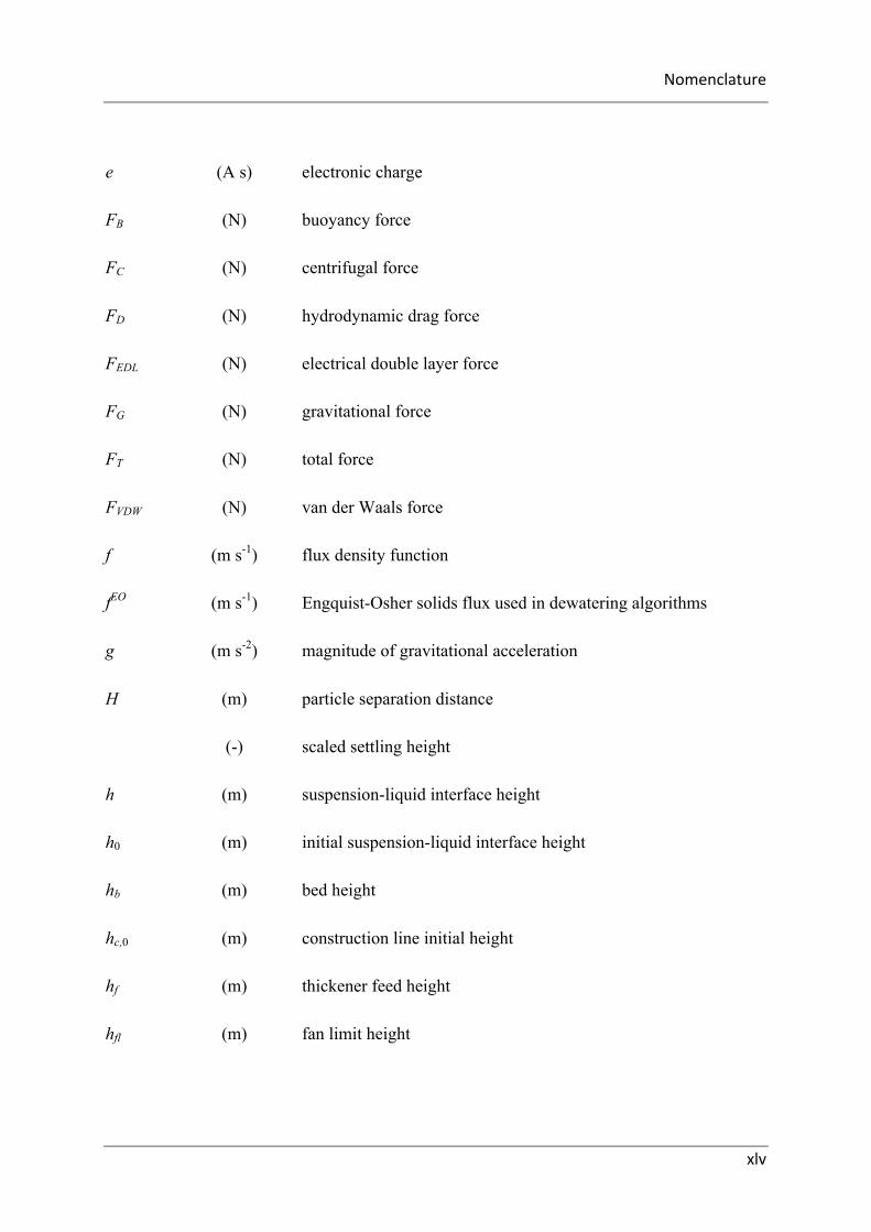
xlv

e (A s) electronic charge

FB (N) buoyancy force

FC (N) centrifugal force

FD (N) hydrodynamic drag force

FEDL (N) electrical double layer force

FG (N) gravitational force

FT (N) total force

FVDW (N) van der Waals force

f (m s-1) flux density function

fEO (m s-1) Engquist-Osher solids flux used in dewatering algorithms

g (m s-2) magnitude of gravitational acceleration

H (m)

(-)

particle separation distance

scaled settling height

h (m) suspension-liquid interface height

h0 (m) initial suspension-liquid interface height

hb (m) bed height

hc,0 (m) construction line initial height

hf (m) thickener feed height

hfl (m) fan limit height

Nomenclature

xlvi

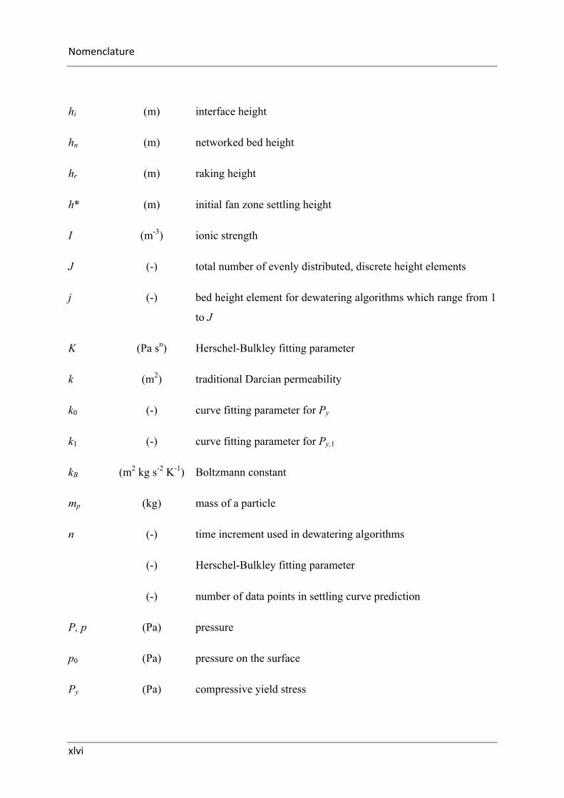
hi (m) interface height

hn (m) networked bed height

hr (m) raking height

h* (m) initial fan zone settling height

I (m-3) ionic strength

J (-) total number of evenly distributed, discrete height elements

j (-) bed height element for dewatering algorithms which range from 1

to J

K (Pa sn) Herschel-Bulkley fitting parameter

k (m2) traditional Darcian permeability

k0 (-) curve fitting parameter for Py

k1 (-) curve fitting parameter for Py,1

kB (m2 kg s-2 K-1) Boltzmann constant

mp (kg) mass of a particle

n (-)

(-)

(-)

time increment used in dewatering algorithms

Herschel-Bulkley fitting parameter

number of data points in settling curve prediction

P, p (Pa) pressure

p0 (Pa) pressure on the surface

Py (Pa) compressive yield stress

Nomenclature

xlvii

Py,0 (Pa) undensified compressive yield stress function

Py,1 (Pa) densified compressive yield stress function

Pbase (Pa) solids network pressure at the base of the settling cylinder

q (m s-1) solids flux

q0 (m s-1) feed solids limiting flux

qfs (m s-1) free settling limited solids flux

qmin (m s-1) minimum solids flux

qmax (m s-1) maximum solids flux

qs (m s-1) sedimentation limited solids flux

qs,min (m s-1) minimum sedimentation limited solids flux

q s,max (m s-1) maximum sedimentation limited solids flux

R (Pa s m-2) hindered settling function

R0 (Pa s m-2) undensified hindered settling function

Rep (-) particle Reynolds number

r (-)

(-)

hindered settling factor

r-direction in spherical coordinates

ra (-) curve fitting parameter for R

ragg (m) aggregate radius

rb (-) curve fitting parameter for R

Nomenclature

xlviii

rc (m) centrifugal radius

rg (-) curve fitting parameter for R

rn (-) curve fitting parameter for R

rp (m) particle radius

S (m3) rake shape factor

S0 (m-3) initial rake shape factor

T (K)

(-)

temperature

scaled time

t (s) time

tb (s) solids residence time within the suspension bed

tcalc (s) time datum point on predicted curve

texp (s) time datum point on experimental curve

tn (s) solids residence time at the networked bed height

tp (m) particle thickness

Tq (N m) torque

Tq,0 (N m) zero yield stress torque

tres (s) solids residence time

tres,0 (s) undensified solids residence time

tres,∞ (s) densified solids residence time

Nomenclature

xlix

tstart (s) raking start time

tstop (s) raking stop time

u (m s-1) settling velocity

u0 (m s-1) undensified hindered settling velocity

u1 (m s-1) fluid flow within aggregates

u2 (m s-1) fluid flow around aggregates

u∞ (m s-1) terminal settling velocity

ufs (m s-1) free settling velocity

ur (m s-1) velocity in the r-direction

us (m s-1) sedimentation limited settling velocity

uΦ (m s-1) velocity in the Φ-direction

uθ (m s-1) velocity in the θ-direction

V (m3) volume

v (m s-1) centrifugal velocity

Vp (m3) average floc or particle volume

x (-) direction coordinate

xφ (m) iso-concentration line height

xφ* (m) initial fan limit settling height via iso-concentration line

z (-) vertical coordinate

Nomenclature

l

zeqm (m) equilibrium bed height

zmin (m) bed height obtained at sedimentation limited solids flux

zi (-) ionic valence of the ith ion

Greek Symbols

α (-)

(-)

thickener diameter correction factor

ratio compressive to shear stress

αv (m-2) specific cake resistance

β2 (m2 s-1) filtration parameter

γ! (s-1) shear rate

γ! (s-1) average shear rate

ΔP (Pa) change in pressure

Δρ (kg m-3) density difference (ρsol-ρliq)

Δσ (Pa) network stress gradient across consolidating solids bed

Δt (s) change in time

Δx (m) change in x direction

Δz (m) change in z direction

δ (m) stern plane

ε (-) safety factor

Nomenclature

li

(-) dielectric constant

ε0 (A2 s4 kg m-3) permeability of free space

ζ (V) electrokinetic or zeta potential

η (Pa s) viscosity

θ (-) θ-direction in spherical coordinates

κ (m) Debye length

κjn (-) parameter for 1-D algorithms presented in Chapter 3

µ (-) mean

ρagg (kg m-3) aggregate density

ρagg,0 (kg m-3) initial aggregate density

ρagg∞ (kg m-3) fully densified aggregate density

ρliq (kg m-3) fluid density

ρsol (kg m-3) solids density

σ (Pa)

(-)

stress

standard deviation

τ (Pa) shear stress

τ0 (Pa) shear stress on the surface

τ0,agg (Pa) shear stress on surface of aggregate

τ0,ave (Pa) average shear stress on the surface

Nomenclature

lii

τ0,max (Pa) maximum shear stress on the surface

τ0,sphere (Pa) shear stress on surface of sphere

τ1 (s) initial settling time

τy (Pa) shear yield stress

τy,ave, yτ (Pa) average shear yield stress

τy,max (Pa) maximum shear yield stress

Φ (-) Φ-direction in spherical coordinates

φ (-) solids volume concentration/fraction

φ0 (-) initial solids volume fraction

φ0,opt (-) optimum initial solids volume fraction

φ1 (-) solids volume fraction above the bed

φ2 (-) solids volume fraction at within the bed

φ∞ (-) equilibrium solids volume fraction

φagg (-) solids volume fraction within an aggregate

φagg,0 (-) initial aggregate solids volume fraction

φagg,∞ (-) fully densified aggregate solids volume fraction

φave (-) average solids volume fraction

φbase (-) solids volume fraction at z = 0

Nomenclature

liii

φcp (-) close packing volume fraction

φf (-) final solids volume fraction

φf,ave (-) average final solids volume fraction

φfl (-) fan limit solids volume fraction

φfl,0 (-) undensified fan limit solids volume fraction

φfl,∞ (-) equilibrium densified fan limit solids volume fraction

φg (-) solids gel point

φg0 (-) initial solids gel point

φg,∞ (-) equilibrium densified solids gel point

φi (-) interface solids volume fraction

φjnL (-) parameter for 1-D algorithms presented in Chapters 2

φjnR (-) Parameter for 1-D algorithms presented in Chapters 2

φlimit (-) solids volume fraction at sedimentation/consolidation limit transition

φmax (-) maximum potential solids volume fraction

φmin (-) minimum potential solids volume fraction

φprefan (-) solids volume fraction within the pre-fan

φs (-) sedimentation limited solids volume fraction

φu (-) underflow solids volume volume fraction

Nomenclature

liv

φ∗ (-) initial solids volume fraction within the fan region

ϕ (-) aggregate volume fraction within a suspension

ϕp (-) aggregate packing fraction at the gel point

χBC (-) drag coefficient correction factor for slip boundary condition

χint (-) drag coefficient correction factor for intermediate flow regime

χNewton (-) drag coefficient correction factor for Newton flow regime

χRep (-) overall drag coefficient correction factor for flow regime

ψ (V) electrical surface potential

ψ0 (V) initial electrical surface potential

ψδ (V) electrical surface potential at the Stern plane

ω (rpm) rake rotation rate

Nomenclature

lv

Abbreviations

1D one-dimensional

CFD computational fluid dynamics

CFL Courant-Friedrichs-Lewy

DLVO Derjaguin, Landau, Verwey, Overbeek

EDL electrical double layer

max maximum

min minimum

MW molecular weight

NR no stationary rake

PE performance enhancement

pH potential hydrogen

PVM particle vision measurement

SR stationary rake

SST steady state thickener

TBS transient batch settling

UV ultra violet

VDW van der Waals

Nomenclature

lvi

Units

cm centimetre

hr hour

J joule

kg kilogram

M molar concentration

m metre

min minute

mm millimetre

N Newton

Pa pascal

rpm revolutions per minute

s second

v/v solids volume fraction

µm micron/micrometre

1

Chapter 1. THESIS OVERVIEW

Chapter 1

Thesis Overview

1.1 Background

Many industries, including minerals, pulp and paper, dairy, water and waste water, require

solid-liquid separation, otherwise known as dewatering as an integral part of operations.

These industries generally tend to create a significant amount of liquid with suspended solids

as waste each year (Boger 2009). As an example, within Australia, 20 million tonnes of

Alumina was produced from bauxite in 2015, accounting for 17 % of world production (BGS

2015). This corresponds to approximately 40 million tonnes of waste tailings. Along with

environmental and safety considerations, this provides motivation for research into

dewatering and solid liquid separations.

Dewatering is performed with two different aims, either thickening of the particulate phase or

clarification of the liquid phase. In some operations, both outcomes are desirable and often

the terms clarification and thickening are used interchangeably. Thickening is performed in

order to increase the solids concentration within the suspension by the removal of the fluid,

most commonly water, while clarification aims to remove finely dispersed particles within a

fluid. The suspension with increased solids concentration is then either sent for further

processing or disposal while the fluid is commonly recycled in the process. As an example,

within the waste water industry, residual solids are sometimes sent to an incinerator to

Chapter1

2

dispose of where dewatering to concentrations greater than 30% is extremely desirable

(Brechtel and Eipper 1990).

A common process used within the mineral industry is simplified into the following steps.

After mining, the ore firstly undergoes crushing to allow the valuable mineral to be freed

from so-called gangue materials. A separation process then ensues to retrieve the valuable

mineral from the gangue. Often, both the crushing and separation stages are completed in an

aqueous environment. Once separation is completed, the residual particulate suspension is

dewatered; the recovered water is recycled while the waste material suspensions, referred to

as tailings, are disposed of in settling ponds/dam or an impoundment area. Due to the low

concentration within the tailings and high production rate, tailing dams are large in size

demanding vast areas and often containment becomes costly. As ore grades decline and

liberation requirements produce finer grained tailings, an increase in tailings volume is

consequential. Insufficient dewatering of the tailings can result in both environmental and

economic consequences (Sofra and Boger 2002).

Not only are there environmental and economic concerns associated with tailing disposal, but

also great safety risks. Due to the difficulties associated with containment of such large

volumes of waste, dam rupture and failure are common resulting in loss of human life along

with damage to property and land. On October 4th, 2010, a bauxite tailings dam in Kolontár

in Hungary failed sending up to 1.3 million cubic meters of tailings into settlements via the

Torna creek. The rupture did not only flood 8 square kilometres, but also injured over a

hundred people as well as 10 deceased (Szépvölgyi 2011). More recently, in 2015, a tailings

dam in Brazil burst releasing between 55 and 62 million cubic meters of tailings resulting in

at least 19 casualties affecting the lives of more than 1 million people (Fernandes et al. 2016).

Optimisation of the dewatering process, including modelling and application has the

possibility to provide major improvements in particulate separations, in particular the mineral

industry. Many environmental, safety and economic implications show that dewatering

optimisation and enhancement is extremely valuable. Greater dewatering results in an

increase of solids concentration and has the possibility of reducing waste volume and water

ThesisOverview

3

losses. This allows for a reduction in land required, as well as reduced safety concerns due to

fluidisation of the tailings.

Within industry, many methods for dewatering are employed, including filtration,

centrifugation and gravity thickening. These processes differ in the driving force, be it

gravitational, centrifugal or mechanical. The dewatering method employed will greatly

depend on economic, environmental and safety considerations as well as the required extent

of separation. Often a combination of methods are used in stages (Svarovsky 1990).

Gravity thickening, as its name suggests, uses gravity as the driving force for separation.

Thickening is generally used either on its own or a precursor to further dewatering. It has

several advantages over other methods of dewatering such as an ability to handle high and

fluctuating throughputs, as well as the ability to handle a fluctuating solids concentrations and

mineral composition in the feed. Thickeners are also inexpensive to operate (relative to other

devices) due to their relatively simple design. Although high solids concentrations can be

reached within a thickener, further dewatering may still be required.

Further dewatering after thickening is often achieved via centrifugation or filtration as these

methods both have driving forces that can be greater in magnitude compared to gravity in

thickening. Due to this larger driving force, a higher compressive stress can be applied

resulting in a higher solid volume fraction, if enough time is allowed for the process to reach

equilibrium. The higher solids may be a statutory requirement or be necessary to achieve an

energy balance in incineration, as mentioned previously. Further recovery and recycling of

water can be achieved along with a reduced waste volume. Applying further dewatering after

thickening can help to reduce environmental factors, however, economic constraints usually

drive decision making. The cost of centrifugation and filtration can typically be up to 100

times higher than thickening. Another downside of filtration is that to operate economically, a

concentrated and homogenous feed is desirable (Bemer and Calle 2000).

Different methods of dewatering exist, but the emphasis on the optimisation of gravitational

thickening is the focus of this thesis. Despite this focus, the improved understanding of

suspension dewatering can be applied to all methods of solid-liquid separation.

Chapter1

4

1.2 Gravity Thickening

The idea of exploiting the density difference between solids and fluids has been around for

centuries. Documents dating back to 200 BC suggest that Egyptians used this idea in order to

recover alluvial gold (Burger and Wendland 2001). Today, gravity thickening uses the same

concept, albeit operation and design are more sophisticated and better separation is achieved.

The process generally uses a tank inclusive of a feed at the top, an overflow weir for recovery

of liquor and an underflow for recovery of a thickened particulate suspension.

Dewatering can be performed either to clarify liquor, increase the underflow solids

concentration or both. Hence the tanks in which dewatering occur are often called thickeners,

settlers or clarifies. Essentially they are the same equipment and the name depends on the

main objective for the vessel.

The tanks are often large and shallow with a flat or slightly sloped bottom where the feed is

introduced and two output streams are produced as shown in Figure 1-1. It is possible to run

thickeners as a batch processes; however, a continuous approach is more common. The feed

consists of a dilute particulate suspension. The first product stream is the underflow, which

contains the majority, if not all, of the feed solid particles and has a solids volume fraction,

φu. The second product stream is the overflow, where the separated liquid is recovered. Most

thickeners operate so that no or minimal solids are present in the overflow. The liquid in this

stream is quite often recycled and reused within the upstream process or further processed to

remove dissolved products.

ThesisOverview

5

Figure 1.1: Schematic of a typical gravity thickener

The feed generally consists of small dispersed particles, sometimes even colloidal, and is

passed through a feed well prior to entering the thickener. The feed well serves as a method

to allow for the addition of flocculant to aggregate particles, causing an increased settling

rate. The feed well also provides as a means to reduce the disturbance to the material within

the thickener by decreasing the momentum of the feed stream.

Three distinct zones within a thickener are operationally important and defined depending on

settling method. These zones, from the top of the thickener, include the clarification,

hindered settling, and compression zone, as shown in Figure 1-1. Within the thickener, the

particles settle to the bottom due to gravity and form a bed. The movement of the suspension

bed into the underflow is aided by the use of a rake as well as a little help from the conical

slope of the base of the thickener. As the particles settle and are removed in the underflow,

the top of the thickener becomes a zone in which liquor becomes virtually free of solids.

For further, more detailed workings of thickeners, the reader is referred to texts, such as

Perry’s Chemical Engineer’s Handbook (Green and Perry 2008), the Kirk-Othmer

Encyclopaedia of Chemical Technology (Svarovsky 1997), and the Chemical Engineer’s

Condensed Encyclopaedia of Process Equipment (Cheremisinoff 2000).

ClarificationZone

HinderedSettlingZone

FeedOverflow

(Clearliquid)

Underflow

(Conc.Solids)

FeedWell

RakeConsolidationZone

Chapter1

6

1.3 Raking and Shear Forces

Traditionally, the rake was initially introduced and designed as a means to transport material

to the underflow as it is important to continuously supply sediment to the discharge pump to

prevent both caking (locally high solids concentrations) and channel formation. However

observations indicate that raking causes shear induced dewatering (Novak and Bandak 1994,

Channell et al. 2000, Johnson et al. 2000).

Gentle shear forces have been observed to improve the rate of thickening for flocculated

feeds. An empirical parameter has been attributed to this rate enhancement and is well

known as the permeability enhancement factor (Usher 2002). Such a parameter can be used

to quantify improvements to thickener performance, however, due to the lack of

understanding of physical properties that govern the rate and extent of dewatering, it does not

allow for the quantitative prediction (Usher and Scales 2009). The mechanisms, by which

rakes provide enhancements, to dewatering is not yet fully understood, but ideas such as

channelling, compression by the blades in the direction of flow and aggregate densification,

have been suggested (Gladman 2006).

The concept of aggregate densification is an important one. Aggregate densification occurs

when shear is applied to a weak aggregate structure and if the shear is great enough, the

aggregate goes from an open structure to a more dense and packed structure, resulting in

removal of water from inside the aggregate (See Figure 1-2). Observations of settling tests

indicate gentle shearing by a rake can greatly increase the extent of dewatering (Usher et al.

2009).

Within this thesis, the term “shear” in the context of within a thickener refers to all sources of

shear including, but not limited to raking, aggregate collisions, mixing etc. The term

“raking” refers to the specific application of shear through a mechanical moving rake. Hence

raking is one method to enhance the shear within a thickener.

ThesisOverview

7

Figure 1.2: Schematic of the proposed effect of shear on aggregates. (Usher et al. 2009)

1.4 Motivation for this Work

The idea of exploiting density difference through gravity thickening to separate solids and

liquids is relatively simplistic. Despite this, a thickener model able to predict full-scale

operations is unavailable. Many challenges surrounding thickener modelling exist, with a

large gap in understanding being attributed to our knowledge of the effect of shear on

dewatering through changes in aggregate structure and location distribution.

A review of the literature shows that a lot of research does not consider the effect of changes

in aggregate structure post flocculation on the sedimentation process (Brinkman 1949,

Mueller et al. 1966, Sutherland and Tan 1970, Neale et al. 1973, Tambo and Watanabe 1979,

Li et al. 1986, Li and Fanczarczyk 1988, Chellam and Wiesner 1993, Johnson et al. 1996,

Gregory 1997, Li and Logan 2001, Franks et al. 2004, Gruy and Cugniet 2004). Rather,

research looks to develop an understanding of the effect of aggregate structure; size and

strength determined via flocculation conditions (Gregory 1987, Yeung et al. 1997, Spicer et

al. 1998, Swift et al. 2004).

The motivation for this project is to provide an understanding of shear induced processes in

thickeners and develop experimental methods to produce material parameters that when used

as inputs into thickener models, allow for optimisation of thickener performance. Currently,

thickeners are designed with rakes primarily to transport sediment to the outlet. This work

Chapter1

8

explores the advantages of raking within a thickener and in turn, develops a better

understanding of the role of shear processes. The aim is to answer the following question: In

what settling zone, for how long, and at what shear rate should a rake or shear device be

operated within a thickener to achieve maximum dewatering performance?

1.5 Research Objective

The objective of this research is to further understand the role shear plays in dewatering. The

research will focus on providing a method for extracting parameters relating to shear induced

dewatering and using these parameters as inputs into dewatering models.

Furthermore, this project aims to provide a guide to thickener operation in relation to raking

operating conditions. This will be achieved through providing insight into determining how

long and at what rate raking needs to be performed to achieve maximum thickener throughput

for a given underflow solids concentration.

To answer these questions and accomplish the objective, a number of tasks were undertaken

including:

• Aggregate densification theory was applied to the results of sheared laboratory batch

settling tests in order to quantify the effects of shear on aggregate densification.

These experiments were aimed at understanding aggregate densification

dependencies. Dependencies included shear rate, localised solids concentration and

particulate network stress.

• Existing 1-D transient batch settling models were updated via incorporation of a new

numerical scheme, which allows for reduced simulation times.

• A 1-D steady state thickening model was developed that incorporates the time

dependency of aggregate densification. This was used to further understand the

discrepancies between current models and industrial observations.

• The above tasks were combined to demonstrate the procedure to predict full-scale

thickener performance from laboratory scale characterisation.

• Practical applications towards process optimisation are discussed and impact of

process variables quantified.

ThesisOverview

9

Although the main objective of this work is to facilitate optimised thickener performance

through increased knowledge of aggregate densification, the limitation of aggregate breakage

exists. This work assumes that shear effects positively influence thickener performance and

the concept and effect of aggregate breakage is not investigated. It should be noted that

aggregate breakage is expected to be important and lead to a decrease in the rate of

dewatering. The likely consequence of ignoring this effect is discussed briefly at a latter

juncture.

Other issues not covered but likely important to a comprehensive analysis of this problem

include polydispersity and particle size distributions. Investigations of these issues would

consider as examples, the effect of particle segregation on thickener performance.

As mentioned earlier, the understanding of the role shear plays within gravity thickening can

be applied to other dewatering methods. However, the transfer of this knowledge to other

dewatering applications is not covered herein.

1.6 Thesis Outline

This thesis is intended to help further understand and explain dewatering behaviour of

aggregated (flocculated) particulate suspensions under shear and applying this knowledge to

investigate the effect on thickener performance. This work is broken into 7 chapters, as

described below:

In Chapter 1, the incentive for research in dewatering processes is considered and in

particular, thickening and its importance to the minerals and other industries. The research

objectives and scope of the thesis are defined.

Chapter 2 outlines the theory used as a base for this work. Dewatering fundamentals are

outlined, followed by a description of the current aggregate densification theory and the

models used to describe and predict dewatering with densification. The outline and summary

of dewatering fundamentals are reviewed including the evolution of dewatering theory along

with the material properties that describe dewatering. The experimental methods used to

determine these properties are also considered. The effect of aggregate densification on

Chapter1

10

dewatering parameters is important and hence typical effects are shown for demonstration.

Current computational algorithms and modelling theory are also presented to show how the

theory of aggregate densification and dewatering theory can be used to predict both batch

settling and continuous thickener operations.

Chapter 3 describes a new computational algorithm used to predict one dimensional (1D)

steady state thickening (SST) with the incorporation of dynamic aggregate densification. The

development of this model is based on sedimentation and densification theory. This model is

subsequently used to predict thickener throughput based on material properties representative

of a mineral slurry. The impact of operational variables is also presented.

Chapter 4 introduces raked batch settling experiments that are consequently used to

characterise materials through aggregate densification. This chapter extracts aggregate

densification parameters from simple methods and describes their behaviour and

dependencies.

Chapter 5 highlights the full package, from laboratory scale material characterisation tests to

full thickener operational prediction. This chapter utilises material characterisation results

from Chapter 4 as inputs into the developed 1D SST model in Chapter 3. A novel method of

obtaining a densification rate due to sedimentation is also presented and applied within model

predictions.

Chapter 6 utilises the experimental observations in Chapter 4 and the steady state thickener

model developed in Chapter 3 to further discuss practical applications. A novel method of

determining the rake torque and shear yield stress based on underflow rheology has been

presented to aid in determination of underflow limitations. Response curves resulting from

investigating the impact of process variables are also presented to further understand

optimisation methods.

Chapter 7 summarises the major outcomes from experimental reality and theoretical

modelling. An overview of the conclusions and major outcomes of the work is included,

which are than measured against the research objectives. Scope for further research within

this field is also presented.

11

Chapter 2. THEORY

Chapter 2

Theory

A particulate suspension is a mixture of solid particles in a liquid phase, whereby the solids

are visible with a microscope or to the naked eye. If left undisturbed, provided the solid

particles are non-colloidal, they will settle due to density differences between the solid and

liquid phases. Examples of everyday particulate suspensions include; mud (dirt in water),

sand in water and pulp containing juice. Particulate suspensions are of high importance to a

wide range of industries including mining and wastewater treatment. Within the mining

industry, a vast quantity of waste particulate suspensions, termed tailings, are produced.

Increasing the solids concentration through water removal, known as dewatering, can be

performed via gravity thickening, centrifugation, or pressure filtration, and can be a very

important part of an industrial operation.

Gravity thickeners are commonly used within the mining industry to expedite the dewatering

of particulate suspensions due to their ability to handle high throughputs and relatively low

operating costs. Often, thickeners are referred to as the workhorse of the industry due to the

importance of this step in the overall process (Mular and Barratt 2002). To increase the

settling rates of the solids in the suspension, flocculation is commonly performed within a

thickener. Flocculation involves the addition of a binding agent, often polymer, to aggregate

the primary particles in the suspension. Increased aggregate size improves the settling rate

and can dramatically improve separation performance. Thus, understanding the dewatering

Chapter2

12

behaviour of aggregated particulate suspensions is crucial to the thickener operation in

industries such as mining and waste-water treatment.

The first section of this chapter introduces dewatering fundamentals – sedimentation and

consolidation, followed by the fundamentals of modern dewatering theory including material

characterisation techniques. Relevant to this work is the effect of shear on the dewaterability

of a suspension, in particular shear induced structure changes within aggregates. Hence, an

overview of aggregation, including colloidal forces, mechanisms, and the resulting aggregate

structure is presented. The theory behind dewatering enhancement due to aggregate

restructure, known as the phenomena of aggregate densification, is subsequently presented

along with methods for incorporation into modern dewatering theory. The method of

characterising aggregate densification is also presented. With the knowledge of dewatering

and densification theory, current batch settling and thickener prediction models are

summarised.

2.1 Dewatering Mechanics

Two mechanisms exist during the dewatering of a solid-liquid suspension in gravity

thickening, sedimentation, and consolidation. Sedimentation refers to the settling of the solid

particles over time due to the net downward buoyancy force leading to discontinuity between

the liquid and particles. If the concentration of the solids were to be sufficiently high such

that a solids bed is formed, any settling would occur solely through compression or

consolidation of the solids bed under its own weight. Over time, consolidation slows as the

gravitational force due to the particles is matched by the resistive strength of the solids bed

network of particles.

The dewatering mechanism present in any system is greatly affected by the local solids

concentration. Sedimentation is predominant at low solids concentrations, while

consolidation is predominant at high solids concentration. Hence, the phenomena of

dewatering can be categorised as, sedimentation in the hindered settling zone and

consolidation within the solids bed.

Theory

13

2.1.1 Sedimentation

Sedimentation refers to particles that, due to forces acting on them, separate from the fluid in

which they are entrained until an external boundary is met. The force acting on the particles

can be gravitational, centrifugal, or mechanical. This research investigates gravity thickening

and hence will look predominately into the role of the gravitational force. Although a

gravitational force is also applied to the fluid the solid particles in the suspension experience

a greater gravitational acceleration due to the different densities. This causes the solid

particles to settle while the fluid is displaced. The viscosity of the fluid limits the rate of

sedimentation.

Stokes (1851) derived an expression for the terminal velocity, u∞, of an isolated spherical

particle in an infinite Newtonian medium through a simple force balance. A balance of all

the forces acting on a settling particle results in;

(2.1)

where FD, FB and FG are the drag, buoyancy and gravitational forces (N) respectively. Note

that this force balance neglects forces such as osmotic pressure, inter-particle forces such as

van der Waal’s, electrostatic repulsion, bridging and steric forces as well as Brownian motion

(Lester 2002). The buoyant force, FB is the force arising due to the displacement of fluid

caused by the particle. Due to the fluid supporting the weight of the particles, FB is related to

the weight of the displaced fluid such that;

(2.2)

where g is the gravitational acceleration (m s-2), rp is the particle radius (m) and ρliq is the

density of the liquid (kg m-3). FG is the force due to gravity acting on the particles, such that;

(2.3)

GBD FFF =+

liqpB grF ρπ 3

34

=

grF solpG ρπ 3

34

=

Chapter2

14

where ρsol is the density of the solid particle (kg m-3). The drag force, FD, in equation 2.1

represents the hydrodynamic drag that results due to the flow of fluid past the particle,

effectively reducing the settling rate of the particle. Stokes determined a solution to FD for a

single spherical particle in an infinite viscous medium in creeping flow. From the equations

of motion, Stokes derived that FD for creeping flow is,

pD ruF ∞= πη6 , (2.4)

where η is the fluid viscosity (N s m-2). As stated, equation 2.4 is valid for creeping flow,

corresponding to a low particle Reynolds number, Rep, such that;

12

Re <<= ∞

η

ρ ur liqpp .

(2.5)

For Reynolds numbers above 0.2, inertial terms become important and an empirical drag

coefficient, CD, is required such that,

2

2projDliq

D

ACuF ∞=

ρ.

(2.6)

where Aproj is the projected cross sectional area of the particle (m2). The drag coefficient has

been measured at a range of particle Reynolds numbers (Lapple and Shepherd 1940). The

results showed the drag coefficient to be a strong function of the particle Reynolds number.

Observed within the results were three distinct settling regimes, defined as the Stokes,

intermediate and Newton’s law regions. Application of curve fitting within the three regions,

allows for the drag coefficient to be expressed as a function of particle Reynolds number.

Within the Stokes regime, Rep < 0.1, equating equations 2.4 and 2.6 results in a Stokes drag

coefficient of

CD,Stokes =24Re p

. (2.7)

Within the intermediate regime (0.1 < Rep < 1000), the intermediate drag coefficient, CD,int

can be approximated by (Lapple and Shepherd 1940),

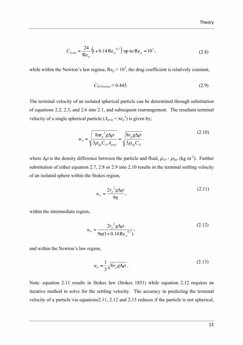
Theory

15

, (2.8)

while within the Newton’s law regime, Rep > 103, the drag coefficient is relatively constant,

CD,Newton ≈ 0.445. (2.9)

The terminal velocity of an isolated spherical particle can be determined through substitution

of equations 2.2, 2.3, and 2.6 into 2.1, and subsequent rearrangement. The resultant terminal

velocity of a single spherical particle (Aproj = πrp2) is given by;

Dliq

p

projDliq

p

Cgr

ACgr

uρ

ρ

ρ

ρπ

38

38 3 Δ

=Δ

=∞ . (2.10)

where Δρ is the density difference between the particle and fluid, ρsol - ρliq, (kg m-3). Further

substitution of either equation 2.7, 2.8 or 2.9 into 2.10 results in the terminal settling velocity

of an isolated sphere within the Stokes region,

η

ρ

92 2 Δ

=∞

gru p ,

(2.11)

within the intermediate region,

)Re14.01(92

7.0

2

p

p gru+

Δ=∞η

ρ , (2.12)

and within the Newton’s law region,

ρΔ≈∞ gru p631 .

(2.13)

Note: equation 2.11 results in Stokes law (Stokes 1851) while equation 2.12 requires an

iterative method to solve for the settling velocity. The accuracy in predicting the terminal

velocity of a particle via equations2.11, 2.12 and 2.13 reduces if the particle is not spherical,

( ) 37.0int, 10Re toup Re14.01

Re24

=+= ppp

DC

Chapter2

16

the fluid is compressible or if there are interactions with other particles within the suspension.

An interconnected particle network in which stress can be transmitted is formed when a

critical solids concentration is reached in which the particles begin to interact. Dewatering

mechanics transition from sedimentation to consolidation at this critical solids concentration.

The critical solids concentration (further discussed in Section 2.4.1) at which this occurs at is

dependent on the suspension and settling vessel.

2.1.2 Consolidation

A density difference between the fluid and solid particles allows for consolidation to occur.

As the concentration of particles increases, a network or gel point concentration will be

observed. When a compressive stress is applied, the particle network is dewatered to a higher

solids volume fraction. An applied compressive stress may cause dewatering by either,

compression of individual particles or aggregates, compression of fluid or compression of the

particle network. The compressibility of the fluid and individual particles are usually

insignificant relative to the compression of the network. Thus, compression of the particle

network dominates consolidation and the fluid and particles are assumed incompressible.

As noted, within a thickener or batch settling test, once a critical solids volume fraction is

reached, a networked bed is formed through which inter-particle forces can transmit.

Applying high enough pressure onto this networked bed will cause failure and hence

consolidation/dewatering. During consolidation the particles become more closely packed

and the fluid travels between the particles towards the top of the bed. Therefore, the

following force balance may represent the consolidation mechanics:

(2.14)

where Δσ is the network stress gradient. Equation 2.14 is also valid for sedimentation

mechanics, where the network stress term is non-existent.

The stress required to consolidate can be applied by various means however within thickeners

and batch settling tests, the bed itself is the most common cause of this stress. The top layer

of the bed exerts a pressure onto the layer below due to self-weight and hence consolidation

GBD FFF =Δ++ σ

Theory

17

of the networked bed occurs. Due to the different gravitational pressures exerted within the

bed as a function of depth, a concentration profile is created within the bed.

2.2 Modern Dewatering Theory

Research into the understanding of dewatering and its behaviour has an extensive history.

For example, as mentioned in Burger and Wendland (2001), the understanding that gold can

be removed through density difference provided economic benefits for the early Egyptians.

A more up to date example shows that the knowledge of dewatering has allowed more

efficient and cost effective thickeners to be built. Early research into dewatering theory was

conducted in order to determine the forces present when a particle settles within a fluid. The

result of this research was Stokes Law as outlined in equation 2.11.

Due to the discrepancies between Stokes Law prediction and actual settling times, research

into the operation of settling tanks was conducted. Coe and Clevenger (1916) considered this

and discovered that the settling rate is largely dependent on the local solids volume fraction,

φ. In other words, the observed variation in the settling velocity upon comparison to the

predictions via Stokes law was due to particle-particle interactions. Settling velocity is

therefore a function of solids concentration and Stokes law only applies for an isolated

particle in an infinite medium. By conducting a series of batch settling tests, Coe and

Clevenger devised a method in which a flux plot could be created showing the relationship

between solids flux and solids volume fraction. While observing and conducting batch

settling tests, Coe and Clevenger also postulated that during settling, distinct sedimentation

and consolidation zones existed, as shown in Figure 2.1.

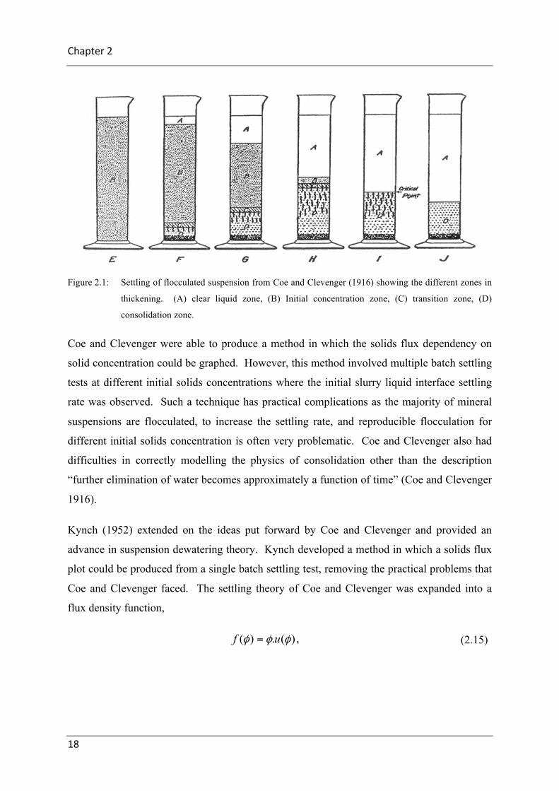
Chapter2

18

Figure 2.1: Settling of flocculated suspension from Coe and Clevenger (1916) showing the different zones in

thickening. (A) clear liquid zone, (B) Initial concentration zone, (C) transition zone, (D)

consolidation zone.

Coe and Clevenger were able to produce a method in which the solids flux dependency on

solid concentration could be graphed. However, this method involved multiple batch settling

tests at different initial solids concentrations where the initial slurry liquid interface settling

rate was observed. Such a technique has practical complications as the majority of mineral

suspensions are flocculated, to increase the settling rate, and reproducible flocculation for

different initial solids concentration is often very problematic. Coe and Clevenger also had

difficulties in correctly modelling the physics of consolidation other than the description

“further elimination of water becomes approximately a function of time” (Coe and Clevenger

1916).

Kynch (1952) extended on the ideas put forward by Coe and Clevenger and provided an

advance in suspension dewatering theory. Kynch developed a method in which a solids flux

plot could be produced from a single batch settling test, removing the practical problems that

Coe and Clevenger faced. The settling theory of Coe and Clevenger was expanded into a

flux density function,

, (2.15) )(.)( φφφ uf =

Theory

19

where f(φ) is the solids volumetric flux (m3 solid m-2 s-1) and u(φ) is the particle velocity

(m s-1). The solid flux density function, f(φ), in equation 2.15 allows for the determination of

the slurry-liquid interface height at different times through a graphical method. In order to

determine the solid flux density function, a continuity equation was proposed;

, (2.16)

where z describes the vertical coordinate of the particle. While developing the above

continuity equation, 2.16, it was assumed that once a certain concentration is reached, φg, all

sedimentation stops and the networked bed is incompressible. In other words, no

consolidation effects are taken into account. This assumption is not valid for most real

systems; however Kynch’s method was still able to explain transient sedimentation behaviour

with the need for only one settling test. For a column of height h0 and initial homogeneous

concentration φ0, a set of boundary conditions can be described in order to solve equation

2.16;

00),(0),0(

0)0,(

0

00

>=

>=

<<=

tthtt

hzz

g

φ

φφ

φφ

. (2.17)

Solving of the continuity equation is possible through an iso-concentration characteristic

method. A solution is obtained where along a characteristic, φ is constant along the straight

lines propagating from the boundary, z = h0;

∫=−=t

tdtuhtz

00 )()( φ , (2.18)

and straight lines propagating from the boundary, z = 0;

. (2.19)

0)( =∂

∂+

∂

∂φ

φ fzt

∫= ∂∂

=t

t

dtftz0

)()( φφ

Chapter2

20

The initial settling region is defined by equation 2.18 for the initial solids concentration, φ0.

Once this settling line intersects the characteristic given by equation 2.19 for φ0, a

discontinuity arises, resulting in a non-linear settling region defined as the fan region. The

fan region continues until the suspension is at φg. The nonlinear settling behaviour within the

fan region is defined by the intersection of the lines in equations 2.18 and 2.19 for all solids

concentrations between φ0 and φg. The transition between settling regions within a batch

settling test is dependent on the initial solids concentration and the materials flux density

function. Up to 7 modes of batch settling have been identified. For further information

regarding the different settling modes refer to Bustos and Concha (1988), Bustos et al. (1999)

and (Lester et al. 2005).

As mentioned, Kynch’s theory assumes that once a suspension reaches φg, consolidation does

not ensue. In real systems, this is not the case due to the solids network creating a self-

initiated stress onto the bed below, allowing for an increase in solids concentration. This

suggests that Kynch theory is valid up to the gel point, however, this is not the case due to the

effect of the build-up of the networked bed at the base on the sedimentation zone (Lester et

al. 2005). Hence, an analytical limit for Kynch theory is defined as the so called fan limit, φfl.

Validation of Kynch’s theory was considered by numerous authors (Shannon et al. 1963,

Tory and Shannon 1965, Shannon and Tory 1966, Davis et al. 1991, Chang et al. 1997);

through the use of glass beads to represent hard spheres in which network consolidation is not

possible. The authors found excellent agreement with Kynch but made no advancement in

addressing the omission of consolidation from the theory. On the other hand, work by

Michaels and Bolger (1962) and Gibson et al. (1967) managed to define the compressive

yield capacity of a networked suspension although they were not able to combine

sedimentation and consolidation theory. Modification of the flux density function as an

extension of the work of Michaels and Bolger was achieved by Fitch (1966, 1983), but still

did not unify sedimentation and consolidation theory.

Buscall and White (1987) were able to define the fundamental theory of dewatering through

the examination of an element of suspension in a vertical force balance, including

gravitational and hydrodynamic forces balanced by the solids pressure gradient. As a result,

Theory

21

they defined three underlying materials properties that govern dewaterability, namely the

compressive yield stress, Py(φ), the hindered settling function, R(φ), and gel point, φg.

Buscall and White (1987) along with Concha and Bascur (1977) changed the way in which

dewatering research is conducted, signifying the beginning of modern dewatering theory.

Although Buscall and White were able to develop the idea of underlying material properties,

quantifying such properties created a problem. This lead to the development of models by

numerous authors (Landman et al. 1988, Landman and White 1994, Garrido et al. 2003)

resulting in a conservation equation;

, (2.20)

where D(φ) is the solids diffusivity (m2 s-1). Note that equation 2.20 assumes a one-

dimensional process in which compression is irreversible. Also note that the solids

diffusivity is a function of both the compressive yield stress and hindered settling function as

described later in section 2.4.5. In the case of no compression, the solids diffusivity goes to

zero. Equation 2.20 also includes a flux term, q(t), which is zero for batch settling and non-

zero for filtration and thickening. Equation 2.20 becomes the same equation as derived by

Kynch, equation 2.16, under conditions of zero flux (batch settling) and no compression

(D(φ) = 0).

2.3 Shear Rheology

A simple measure of fluid flow is the concept of a fluid viscosity developed by Newton (Bird

et al. 2006). Fluid viscosity, η, is defined as the shear stress, τ, divided by the shear rate, !γ ,

where the shear rate is the velocity gradient, du/dz.

The simplest rheological behaviour is of a Newtonian fluid, where the viscosity is constant

over a wide range of shear rates. Non-Newtonian fluids have a viscosity that varies with

shear rate, but can also vary with time as well as the shear and temperature history of the

material. The rheological behaviour of particulate suspensions is considered time

( ) ( ) ( )⎥⎦⎤

⎢⎣

⎡ ++∂

∂

∂

∂=

∂

∂φφ

φφ

φ ftqz

Dzt

Chapter2

22

independent when rheological properties are a reproducible function of shear rate and do not

depend on the material’s shear history (Pashias 1997).

For particulate suspensions at high enough solids concentrations, the flow behaviour is

between that of a solid and liquid (Nguyen and Boger 1992). This behaviour is characterised

by the presence of a critical shear stress, known as the shear yield stress, τy. At shear rates

below the shear yield stress, the suspension does not flow, but instead deforms plastically

(Nguyen and Boger 1992). At shear rates above the shear yield stress, the suspension yields

and flows like a liquid with a viscosity that varies with shear rate. This section overviews

shear rheology characterisation methods and constitutive models. For more detailed review

of shear rheology and in particular particulate suspension rheology, beyond the scope of this

thesis, the reader is directed to the work of Pashias (1997), Metzner (1956), Cheremisinoff

(1986) and Barnes et al. (1989).

2.3.1 Shear rheology characterisation

Shear rheology characterisation in terms of shear stress vs. shear rate behaviour and the shear

yield stress can be determined by many techniques including concentric cylinder rheometry

with the bob rotating in an infinite media suspension or very large gap (cup and bob) and the

vane technique (Nguyen and Boger 1985). Determination of the shear stress vs. shear rate

and shear yield stress can be determined via experiments using these techniques at a range of

solids concentration, φ. The resultant shear stress vs. shear rate data can be fitted to empirical

models to describe the rheological behaviour of the suspension.

2.3.2 Shear rheology models

Two commonly used models exist to describe the shear stress vs. shear rate behaviour for

yield stress materials, the Hershel-Bulkley model (Herschel and Bulkley 1926) and the

Casson model (Casson 1959). Work conducted within this thesis employs the Hershel-

Bulkley model.

The Hershel-Bulkley model employs empirical parameters K and n to relate shear stress, τ,

shear rate, !γ , and shear yield stress, τy, according to,

Theory

23

. )()()( )(φγφφτφτ ny K !+=

(2.21)

At the limit of low solids volume fraction, φ ≈ 0, n(φ) approaches 1 while K(φ) approaches

the viscosity of the fluid. Herschel-Bulkley rheology parameters can be fitted to the obtained

shear stress vs. shear rate rheograms for a range of solids concentrations. The dynamic

viscosity, η(φ), can therefore be given by;

. (2.22)

2.4 Dewatering Material Properties

In the theory of Buscall and White (1987), it was suggested that three important material

properties govern dewatering, namely the suspension gel point, compressive yield stress, and

hindered settling function. Along with the flux density function and solids diffusivity, these

properties help to characterise a suspension and will now be described. The experimental

methods by which quantification of these properties is achieved are described in section 2.5.

2.4.1 Gel point

The minimum solids volume fraction at which individual flocs or particles come into contact

to form a continuous networked bed with the ability to support a stress is defined as the gel

point, φg. In other words, the gel point is the maximum solids concentration a suspension can

obtain due to sedimentation alone. Once the gel point has been achieved, due to the

interconnected particle network, a quantifiable strength can be measured subject to the solids

volume fraction.

2.4.2 Compressibility

Compressibility refers to the ability of a suspension to increase in solids volume fraction, φ,

due to an applied stress. To quantify the compressibility of a material, a compressive yield

stress, Py(φ), has been defined, analogous to the shear yield stress. The compressive yield

stress is the maximum stress that can be applied to a suspension at a given solids volume

( ) ( ) ( )( ) ( ) 1−+== φγφ

γ

φτ

γφτ

φη ny K !!!

Chapter2

24

fraction before failure resulting in dewatering to a higher concentration. As a compressive

yield stress is only observed when the suspension has a networked structure, the compressive

yield stress and gel point are inherently related such that,

cpg

gyP φφφ

φφφ

≤<

≤

⎩⎨⎧

>=

00

)( , (2.23)

where φcp is the solids close packing volume fraction. The particles or aggregates of the

suspension are disconnected at concentrations below the gel point and hence stress cannot be

transmitted and the compressive yield stress is zero. Above the gel point, Py(φ) increases

exponentially until the close packing solids concentration, φcp is reached, in which Py(φ) is

determined by the compressive strength of the solid particles and hence can be considered as

infinite. Figure 2.2 illustrates this behaviour.

The determination of the compressive yield stress can be achieved by a variety of tests

including equilibrium batch settling (Lester et al. 2005), centrifugal settling (Buscall and

White 1987, Usher et al. 2013) and pressure filtration tests (de Kretser et al. 2001, Usher et

al. 2001, Stickland et al. 2008). The following equation, described by Lester et al. (2005), has

been shown to be appropriate to model the compressive yield stress as a function of solids

volume fraction for some particulate systems.

( )( )( )

0

0)(k

g

gcpy

baP

−

⎥⎥⎦

⎤

⎢⎢⎣

⎡

−

−+−=

φφ

φφφφφ , (2.24)

where a0, b and k0 are curve fitting parameters. For Figure 2.2, curve fitting parameters of

0.7, 0.01 and 7 were used for a0, b and k0 respectively. Gel point and close packing solids

volume fractions of 0.1 and 0.63 respectively, were also used. Alternative equations used

within literature (Landman et al. 1988) to model the compressive yield stress include;

⎟⎟

⎠

⎞

⎜⎜

⎝

⎛−⎟

⎟⎠

⎞⎜⎜⎝

⎛= 1)(

0

0

k

gy aP

φφ

φ , (2.25)

and

Theory

25

0

1)( 0

k

gy aP

⎟⎟

⎠

⎞

⎜⎜

⎝

⎛−⎟⎟⎠

⎞⎜⎜⎝

⎛=

φφ

φ . (2.26)

The relation between τy(φ) and Py(φ) has been measured experimentally for a number of

systems (Buscall et al. 1987, Meeten 1994, Channell and Zukoski 1997, Green 1997, Zhou et

al. 2001, de Kretser et al. 2003, Kristjansson 2008, Spehar 2014) and generally follows a

constant ratio, α, such that,

)()(

φτ

φα

y

yP= . (2.27)

Figure 2.2: Typical compressive yield stress, Py(φ), as a function of solids volume fraction, φ. (A) Linear

coordinates and (B) Semi-logarithmic coordinates (Adapted from Usher (2002)).

2.4.3 Permeability

During dewatering, the solid particles experience a drag force due to the interactions with the

liquor as it flows past, causing hydrodynamic resistance to flow. The permeability of a

suspension is inversely related to the hydrodynamic resistance and influences the rate of

dewatering. Permeability and the resistance of flow through a suspension can be defined and

quantified by many different methods. Most commonly defined parameters, but not limited

0

50

100

150

200

250

300

0 0.05 0.1 0.15 0.2 0.25 0.3 0.35 0.4

Compressiv

eYieldStress,P

y(φ)(kPa)

SolidsVolumeConcentranon,φ,(v/v)

1.E-03

1.E-02

1.E-01

1.E+00

1.E+01

1.E+02

1.E+03

0 0.05 0.1 0.15 0.2 0.25 0.3 0.35 0.4

Compressiv

eYieldStress,P

y(φ)(kPa)


0

0.5

1

0.05 0.1 0.15

Py(φ

)(kPa)

φ,(v/v)

GelPoint

Chapter2

26

to, include; the hindered settling function, R(φ), a settling velocity, u(φ), a traditional Darcian

permeability, k(φ), and a specific cake resistance, αv (m-2).

This research will use the hindered settling function method in order to determine and

quantify the permeability of suspension settling. The hindered settling function is a measure

of the hydrodynamic resistance to flow though a suspension, which is inversely related to the

permeability and settling velocity of the suspension.

Stokes Law adequately describes the sedimentation velocity of an isolated particle, but needs

to be modified in order to account for non-isolated particles. A reduction in the settling

velocity occurs due to the presence of long-range hydrodynamic interactions between

particles within a suspension. Early modifications such as those due to Richardson and Zaki

(1954) simply added a constant to Stokes Law to account for non-isolated systems. This

approach was limited in application and Landman and White (1994) introduced a solids

concentration dependence called the hindered settling factor, r(φ). The hindered settling

factor is a fractional representation of how close the ideal Stokes settling velocity, u∞, is to

the actual velocity of the particle, u(φ);

. (2.28)

This function displays the following inherent properties:

. (2.29)

Incorporation of the hindered settling factor, r(φ), to modify the drag force on a particle in a

suspension of material at a solids concentration, φ, results in (Gladman 2006);

)()(1

φφφφ ur

VCFp

DD −= , (2.30)

where Vp is the particle volume (m3). While it is possible to determine the inter-phase drag

coefficient, CD, of ideal fractals (Huilgol et al. 1995), CD and Vp are difficult parameters to

2)1()(

)r( φφ

φ −= ∞

uu

0)(lim1)(lim

1

0

→

→

→

→

φ

φ

φ

φ

rr

Theory

27

determine experimentally for systems with non-ideal fractal aggregates. De Kretser et al.

(2001) defined a hindered settling function, R(φ) due to the difficulty in obtaining the inter-

phase drag coefficient, CD, and particle volume, Vp, for non-ideal fractal aggregates. The

hindered settling function incorporated these difficult to measure parameters as well as the

hindered settling factor as such;

)()( φφ rVCRp

D= , (2.31)

where the hindered settling function can be quantified using,

. (2.32)

Theoretically, determining the hindered settling factor is possible for ideal systems.

Batchelor (1972), determined r(φ) for monodisperse suspension of spheres to first order in φ.

Determination of the hindered settling function is unfeasible for real systems due to the

complex nature of the system causing significant difficulties. Hence, the hindered settling

function, R(φ), is determined experimentally and curve fits such as equations 2.33 and 2.34

have been fitted to a wide range of data (Lester et al. 2005, Usher and Scales 2005);

( )

( ) br

ga

ra

rrrR

rR

n

n

+−=

−=

−

−

φφ

φφ

)(

1)(,

(2.33)

(2.34)

where ra, rn, rg and rb are curve fitting parameters. Details on the methods used to determine

R(φ) experimentally can be found in section 2.5. Figure 2.3 illustrates a typical hindered

settling function as a function of solids volume concentration plot for flocculated

suspensions. Figure 2.3 is based on a curve fit to equation 2.34, with curve fitting parameters

ra = 5×1012, rb = 0, rg = – 0.05 and rn = 5 (Usher and Scales 2005, Usher et al. 2009, van

Deventer et al. 2011, Grassia et al. 2014). It should be noted that the hindered settling

function can become large in magnitude as the solids concentration increases and hence inter-

( )( )φφρ

φugR

21)( −Δ=

Chapter2

28

phase drag is the limiting stage of dewatering resulting in many systems being defined as

permeability limited.

Figure 2.3: Typical hindered settling function plot, R(φ), as a function of solids volume concentration, φ. (A)

Linear coordinates and (B) Semi-logarithmic coordinates. (Adapted from Usher (2002))

2.4.4 Solids flux

The solids flux function, f(φ,t), is defined as a solids volume fraction multiplied by a settling

velocity, equation 2.15. Substituting in equation 2.32 results in the solids flux function in

terms of the hindered settling function, R(φ), according to,

( ))(

1)(.)(2

φφρ

φφφφRguf −Δ

== . (2.35)

Figure 2.4 illustrates a typical solids flux as a function of solids volume concentration for

flocculated suspensions.

0

1E+10

2E+10

3E+10

4E+10

5E+10

6E+10

7E+10

8E+10

9E+10

1E+11

0 0.05 0.1 0.15 0.2 0.25 0.3 0.35 0.4

Hind

ered

Sep

lingFuncno

n,R(φ)(kgs-

1 m-2)


1.00E+06

1.00E+07

1.00E+08

1.00E+09

1.00E+10

1.00E+11

0 0.05 0.1 0.15 0.2 0.25 0.3 0.35 0.4Hind

ered

Sep

lingFuncno

n,R(φ)(kgs-

1 m-2)


Theory

29

Figure 2.4: Typical solids flux vs. solids concentration for a flocculated mineral slurry. Graph produced

using a density difference, Δρ = 2200 kg m-3, and equation 2.34 to describe the hindered settling

function with parameters values, ra = 5x1012, rg = -0.05, rn = 5 and rb = 0.

2.4.5 Solids diffusivity

A property commonly used in filtration, namely the solids diffusivity, D(φ), combines the

effects of compressibility and permeability into a single term. The solids diffusivity is

directly related to the compressive yield stress, Py(φ), and the hindered settling function, R(φ),

such that;

( ))(

1)()(2

φφ

φ

φφ

RddP

D y −= . (2.36)

As shown in equation 2.36, the solids diffusivity is inversely related to the hindered settling

function, implying that a suspension of high solids diffusivity has greater dewaterability.

0.E+00

1.E-05

2.E-05

3.E-05

4.E-05

5.E-05

6.E-05

0 0.05 0.1 0.15 0.2

SolidsF

lux,f(φ)(m

s-1 )

SolidsConcentranon,φ(v/v)

Chapter2

30

This is not always the case due to the dependence on the compressive yield stress and as

such, using the diffusivity as a means of gauging the material properties should be done with

care.

2.5 Dewatering Material Properties: Characterisation

Material properties, such as the compressive yield stress, Py(φ), hindered settling function,

R(φ), gel point, φg, and solids diffusivity, D(φ), are very system specific due to differences in

particle size, material density and flocculation. They need to be determined experimentally.

The most common material property characterisation techniques involve transient and

equilibrium batch settling and pressure filtration tests although other methods such as

centrifugation and gravity permeation are also useful. Due to the large range in concentration

over which material properties can occur, a combination of experimental methods is often

required to determine the complete functional form, 0 < φ < 1. Most commonly, as a

minimum, batch settling tests are combined with pressure filtration experiments to determine

material properties at low and high solid concentrations respectively (Lester et al. 2005).

A description of standard methods and theory used for material property characterisation in

this thesis are now presented.

2.5.1 Batch settling

A significant amount of data can be obtained from the moderately simplistic method of batch

settling. A batch settling test consists of filling a cylinder with a suspension at a given initial

and uniform solids concentration and allowing it to settle due to gravity. This simple method

allows for a comprehensive analysis to be performed. Two data analysis methods are

available, namely transient and equilibrium analysis. Transient analysis, as its name

suggests, takes the suspension interface height over time, and determines the hindered settling

function. Additionally, equilibrium analysis, utilizing the final bed height and pressure

filtration data, is used to determine the compressive yield stress and the networked gel point.

Due to the low network pressure associated with batch settling tests (relative to filtration), the

compressive yield stress, and hindered settling function determined from this analysis is

restricted to low solids concentrations.

Theory

31

Due to characterisation methods, knowledge of the compressibility of the suspension at high

solids volume fractions, via pressure filtration, is required before batch settling equilibrium

analysis can be performed. Transient batch settling analysis requires the knowledge of the

solids gel point, φg, and hence is to be performed after equilibrium batch settling analysis.

2.5.1.1 Transient batch settling analysis

Transient batch settling analysis is used to determine the hindered settling function of the

suspension through analysis of transient height against time data. The hindered settling

function from batch settling tests at low solid concentrations is calculated using;

. (2.37)

As outlined earlier, Kynch (1952) proposed a graphical method in which a batch settling

curve can be constructed from a material flux plot. The reverse is possible, where an

experimentally determined settling curve can be used graphically to determine the material

flux values at φ0 > φ > φg. Through the method of Kynch (1952), interface heights are used to

determine the settling rate, u(φ), through exploiting the fan of iso-concentration curves.

Usher et al. (2013) proposed an adaption of this method involving the following easy to apply

steps:

For a given solids concentration, φi, the corresponding initial height, hi(0) is

determined through the material balance,

. (2.38)

On a graph of height vs. time, h(t), a straight line is constructed from the point (0,

hi(0)) to tangentially intersect the settling curve at (ti, h(ti)). The gradient of the

constructed curve is the settling velocity, u(φi), such that,

)()1()(2

φφρ

φugR −Δ

=

ii hh 00φφ =

Chapter2

32

i

iii t

thhu )()0()(

−=φ . (2.39)

This process is repeated for different solid concentrations until a settling velocity is

acquired for the range of solid concentrations. Increasing the number of solid

concentration points analysed will increase the accuracy of the material flux

functional form. With the settling velocity data and using equation 2.15, a material

flux function can be determined. Using equation 2.32 the hindered settling function

can also be determined.

The graphical method of Kynch (1952) and adaption by Usher et al. (2013) involves

constructing the flux density function, f(φ), and corresponding settling velocities. Lester et al.

(2005) developed a method in which the hindered settling function could be directly obtained

from the settling curve. Lester’s method involved fitting an analytical expression to the

settling curve, and through inversion, the flux function can be determined. Both methods are

indistinguishable when applied to mineral slurries providing the correct analytical limits are

applied (van Deventer 2012). Settling velocities are then converted to R(φ) through equation

2.32.

Kynch defined the analytical limit of batch settling analysis as the solids gel point, φg, which

is valid only for incompressible materials. For compressible materials, Lester et al. (2005)

defined the fan limit concentration, φfl, as the maximum concentration before the build-up of

the bed starts to affect the dynamics of the settling behaviour and hence the analytical limit

for batch settling tests. The fan limit concentration is defined as;

, (2.40)

where f(φ) is the solids flux according to equation 2.15. Grassia et al. (2011) defined a

simpler method. This method allowed for the fan limit to be determined without the need for

the reconstruction of the flux function. Only the gel point and transient settling data is

required. For an incompressible bed with a uniform concentration, φg, and a linear bed

gfl

flfl ffφφ

φ

φ

φ

−=

∂

∂ )()(

Theory

33

growth, the fan limit, hfl can be obtained from the intercept of the actual bed thickness and the

height-settling curve, through a mass balance;

. (2.41)

2.5.1.2 Equilibrium batch settling analysis

Equilibrium analysis allows for the determination of the gel point and compressive yield

stress through an equation based approach. Once equilibrium is reached, no further

consolidation takes place and the solids network pressure within the bed is equal to the

compressive yield stress;

, (2.42)

where p is the solids network pressure within the bed (Pa). The pressure gradient within a

networked bed is a function of gravitational acceleration, the solid liquid density difference

and the solid volume fraction such that;

, (2.43)

re-arranging,

. (2.44)

The solids network pressure at the base of the bed, z = 0, is;

, (2.45)

By definition the pressure at the top of the bed, z = hb, is zero. Substituting this boundary

condition and the boundary condition of equation 2.45 as well as equation 2.42;

gfl

hhφφ 00=

)(φyPp =

φρgdzdp

Δ−=

∫∫−

Δ= dp

gdz

φρ11

00φρghpbase Δ=

Chapter2

34

. (2.46)

Using a functional form for Py(φ), for example equation 2.24, rearranging and substitution

into equation 2.46 allows for a numerical approach where the curve fitting parameters and the

gel point can be manipulated until prediction of the bed height, hb, matches the

experimentally obtained bed height.

2.5.2 Centrifugation

Sedimentation is the result of an external force being applied to a suspension. In the case of

batch settling, this is gravity. Centrifugation is a commonly used method to increase the

magnitude of the gravitational force and hence increase the rate of sedimentation. Therefore,

centrifugation can provide details of the compressive yield stress, Py(φ), and hindered settling

function, R(φ), at solid concentrations greater than that obtained from batch settling.

Commonly, centrifugation is omitted from full characterisation, as the combination of batch

settling and filtration provides enough data to create a full material property profile. The

centrifugal force can be expressed as

, (2.47)

where FC is the centrifugal force (N), v is the velocity (m s-1), rc is the circular radius (m) and

mp is the mass of the particle (kg). The analysis method for centrifugation is similar to that of

batch settling, however the gravitational force is now replaced with equation 2.47 (Buscall

and White 1987, Usher et al. 2013).

2.5.3 Pressure filtration

A networked bed within a thickener has a pressure gradient throughout due to self-weight;

consolidation occurs resulting in a solids concentration gradient where high solids

concentrations are experienced towards the bottom of the thickener. Consequently, material

characterisation needs to be performed at higher solid concentrations than achievable via

∫Δ

−

−

Δ=

0

10

)(11

φρρogh y

b dppPg

h

cpc rvmF2

=

Theory

35

batch settling and centrifugation tests. A lot of work has gone into developing pressure

filtration as a technique to determine compressive yield stress and hindered settling function

for solid concentrations above the gel point (Landman et al. 1995, Green and Boger 1997,

Green et al. 1998, Aziz et al. 2000).

Pressure filtration test methods are not as simple as batch settling tests, but important, and a

significant quantity of data is still obtained as it allows for compressional effects to be

incorporated (de Kretser et al. 2001, Usher et al. 2001, Lester et al. 2005). Pressure filtration

tests consist of filling a cylinder with a sample of initial concentration, φ0, and height, h0, and

subjecting it to an applied constant pressure. This applied pressure forces dewatering to

occur and fluid to pass through a permeable membrane at the base of the cylinder. A cake

also builds up from the base of the cylinder (i.e. at the membrane) where the solids

concentration is at equilibrium, φ∞, at the base of the cake and concentrations greater than or

equal to the gel point, φg, at the top.

Reaching equilibrium can take from hours to several days and the tests needs to be repeated

for a range of different applied constant pressures resulting in a long testing time for some

materials. In order to reduce the required testing time, de Kretser et al. (2001) and Usher et

al. (2001) devised a stepped pressure filtration device and method where R(φ) and Py(φ) can

be determined in minimal time as well as allowing for time dependent materials to undergo

real time optimization of filtration and characterization. A schematic of the step pressure

filtration device is shown in Figure 2.5.

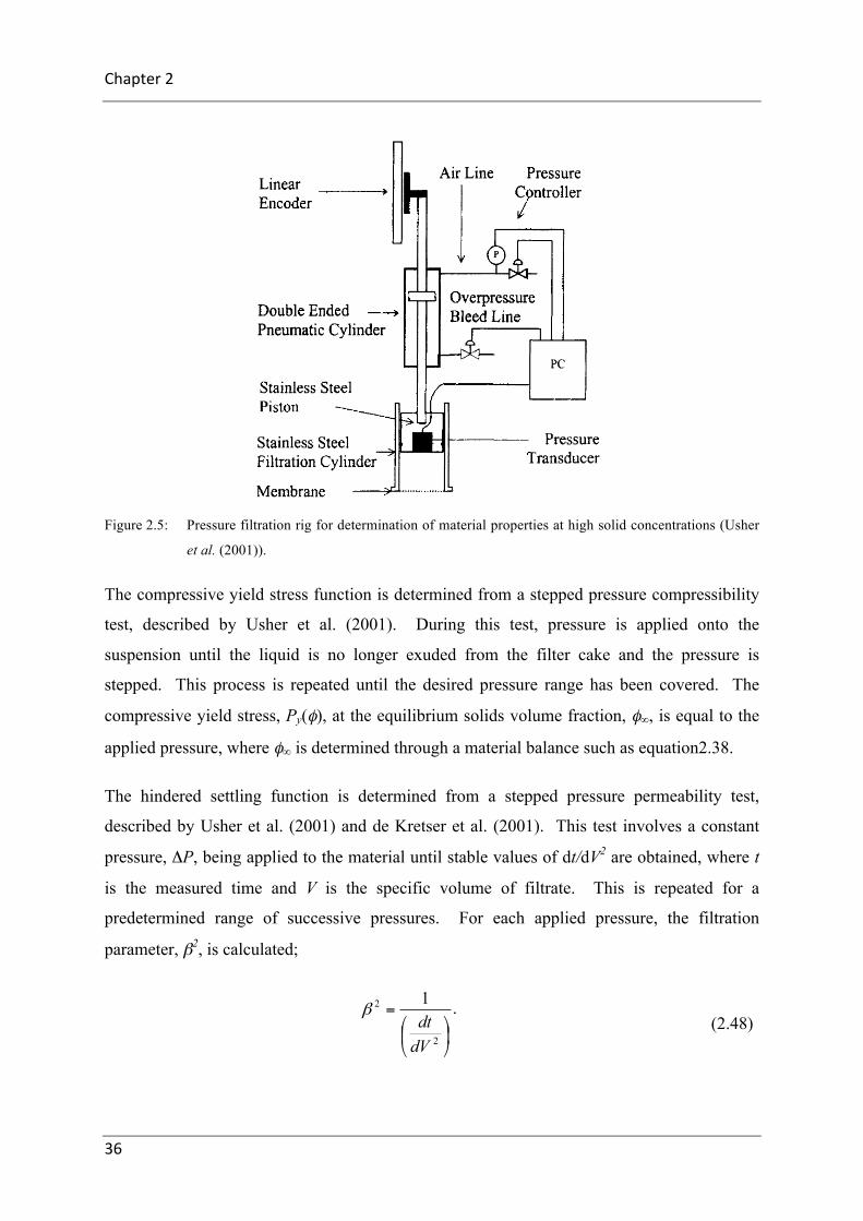
Chapter2

36

Figure 2.5: Pressure filtration rig for determination of material properties at high solid concentrations (Usher

et al. (2001)).

The compressive yield stress function is determined from a stepped pressure compressibility

test, described by Usher et al. (2001). During this test, pressure is applied onto the

suspension until the liquid is no longer exuded from the filter cake and the pressure is

stepped. This process is repeated until the desired pressure range has been covered. The

compressive yield stress, Py(φ), at the equilibrium solids volume fraction, φ∞, is equal to the

applied pressure, where φ∞ is determined through a material balance such as equation2.38.

The hindered settling function is determined from a stepped pressure permeability test,

described by Usher et al. (2001) and de Kretser et al. (2001). This test involves a constant

pressure, ΔP, being applied to the material until stable values of dt/dV2 are obtained, where t

is the measured time and V is the specific volume of filtrate. This is repeated for a

predetermined range of successive pressures. For each applied pressure, the filtration

parameter, β2, is calculated;

. (2.48)

⎟⎠

⎞⎜⎝

⎛=

2

2 1

dVdt

β

Theory

37

The filtration parameter, β2, is plotted against the applied pressure at which it was

determined, ΔP, and a power law curve is fitted. Determination of the gradient of the power

law curve fit allows for the determination of the hindered settling function at high solids

concentration through the equation;

( )20

2 1112)( ∞∞

∞ −⎟⎟⎠

⎞⎜⎜⎝

⎛−

Δ

= φφφβ

φ

Pdd

R , (2.49)

where φ∞ has already been determined for each applied pressure from the compressibility test

data.

2.6 Aggregation

Aggregation is commonly employed to improve the settling rate of particles in industry. Poor

settling predominantly occurs due to the small size of the particles whereby large

hydrodynamic forces dominate over gravitational forces. This domination of hydrodynamic

forces can dramatically slow setting rates, even to a point where Brownian motion inhibits

settling altogether. Aggregation solves this by amassing fine particles into flocs to provide an

increased mass and hence increased gravitational force allowing for higher settling velocities

to be obtained. An increased settling rate allows for increased thickener throughputs to be

achieved (Pearse and Barnett 1980). Aggregation solves the issue of low settling rates but

causes another issue in terms of common dewatering goals. Due to the open nature of flocs,

the bed in a thickener is networked at a lower solids concentration than for an unflocculated

system and given that the upper limit of thickening is usually determined by the suspension

rheology, flocculation can limit the underflow solids concentration. Despite this problem,

aggregate densification provides the opportunity to offset this issue.

Aggregation can be achieved in numerous ways, all allowing for individual fine particles to

amass and bind. The aggregation mechanisms differ depending on the method. Within this

thesis, the focus will be predominately on bridging flocculation by high molecular weight

polymers. Other mechanisms for aggregation include but are not limited to: coagulation,

capillary condensation, and chemical bonding (Fendler 1996). It should be noted that

Chapter2

38

aggregation, flocculation, and coagulation are often used interchangeably within the

literature.

A comprehensive review of inter-particle forces has been extensively covered within the

literature ((Robins and Fillery-Travis 1992, Fendler 1996, Johnson et al. 2000, Hunter 2001)).

Based on readings, a brief introduction into the theory of inter-particle forces is presented to

further discuss the methods for aggregation.

2.6.1 Colloidal forces

This section is provided as an introduction into the surface forces present within suspensions

in order to better understand the effect of these forces on aggregation and as a precursor to

the study of aggregate densification. Colloids are small sized particles where their behaviour

is strongly affected by inter-particle forces. These forces can be either attractive or repulsive

in nature. Major inter particle forces present within colloidal systems include:

• Van der Waals

• Electrical double layer

• Structural (‘hydration’) forces

• Hydrophobic forces

• Steric and electrostatic forces

• Polymer bridging and depletion

A brief definition of these forces is now provided. For a more comprehensive and detailed

description into surface chemistry and forces, the reader is referred to the works of Hunter

(2001), Israelachvili (1991) and Larson (1998).

2.6.1.1 Van der Waals forces

Van der Waals forces are ever present within a suspension as they are due to the

instantaneous dipole moments produced within the atoms of each particle (Israelachvili and

Pashley 1983). Although atoms are non-polar, the shift in the centre of mass of the electron

cloud relative to the positive nucleus allows for the formation of instantaneous dipoles. The

electromagnetic field created due to the instantaneous dipole interacts with neighbouring

Theory

39

atoms causing in induced dipole and so on with other neighbouring atoms. These

instantaneous or induced dipoles arrange in order to reduce their interaction energy however

on a macroscopic scale; these dipoles give rise to a net attractive force in systems where the

density of particles is higher than that of the fluid. Van der Waals forces are inversely related

to the separation distance and hence are of interest for suspensions where there is small

separation between particles. As an example, equation 2.50 (Mahanty and Ninham 1976)

describes the van der Waals force between two flat particles in a fluid with a separation

distance H;

( ) ( ) ⎟⎟

⎠

⎞

⎜⎜

⎝

⎛

+−

++−= 222

2211

12 pp

HVDW tHtHH

AF

π, (2.50)

where FVDW is the attractive van der Waals force (N), AH is the Hamaker costant (J) (Hamaker

1937), H is the separation distance between surfaces (m) and tp is the thickness of the

particles (m).

2.6.1.2 Electrical double layer forces

Within suspensions, particles acquire a surface charge due to the presence of a polar

environment (Caruso 2006). For a mineral oxide particle (M) in water, substitution, surface

site dissociation or adsorption of hydrogen (H+) and hydroxyl (OH-) ions takes place (Healy

and White 1978, Everett 1988);

. (2.51)

The substitution/adsorption of ions results in a net positive or negative charged surface where

oppositely charged ions are attracted and like ions repelled. Overall an ionic neutralisation of

the surface charge over a short distance is experienced where the co and counter ions in

solution are distributed unevenly, although not randomly, as shown in Figure 2.6 (A).

These molecular interactions cause two regions or layers to be created, namely the Stern and

diffuse layer as shown in Figure 2.6. The Stern layer is the inner layer in which oppositely

charged ions are tightly bound to the surface of the particle. This layer has a thickness of

+− −↔−↔−++

−

+

− 22 OHMOHMOMOHH

OH

H

OH

Chapter2

40

approximately one hydrated ion diameter with the outer boundary known as the Stern plane

(Robins and Fillery-Travis 1992). A shear plane is present at the boundary between the Stern

and diffuse layers of the electrical double layer. On the particle surface side of the shear

plane, water molecules and ions are effectively immobilised during particle motion.

The diffuse layer comprises of dispersed ions that are attracted due to a coulomb force. The

thickness of the electrical double layer is characterised by the Debye length, which represents

the length scale of the electrical double layer. The Debye length is often determined as the

length in which a decrease of one exponential factor in the surface potential occurs (Hunter

2001). For a simple symmetrical electrolyte species, the Debye length, κ-1, can be calculated

as (Hunter 2001);

, (2.52)

where Ι istheionicstrengthofthebulksolution,determinedvia;

∑=

=i

iii zCI

1

2

21 , (2.53)

where e is the electronic charge, ε0 is the permeability of free space, ε is the dielectric

constant of the bulk solution, kB is the Boltzmann constant, T is the temperature, zi is the ionic

valence of the ith ion and Ci is the concentration of the ith ion. The arrangement of co and

counter ions affects the magnitude of the surface potential; ψ. Figure 2.6 (B) demonstrates

the change in electrical potential over the electrical double layer. Initially the surface

potential, ψ0, decreases linearly up to the Stern plane, where the electrical potential is ψδ. As

distance is increased from the Stern plane, the electric potential decreases exponentially to

zero. The shear plane electrical potential is called the zeta potential, ζ, often used as the

charge of a particle in electrokinetic studies.

21

0

21 2

−

−

⎟⎟⎠

⎞⎜⎜⎝

⎛=

TkIeBεε

κ

Theory

41

Figure 2.6: The electrical double layer effect on a negatively charged particle (A) ionic distribution and (B)

electrical surface potential as a function of distance from the particle surface (Adaptation from

Green (1997)).

When two particles come into range such that the electrical double layers overlap, a high

concentration of ions between the surfaces occur compared to the bulk solution. This

increase in concentration of ions produces an increase in osmotic pressure and free energy

resulting in a repulsive inter-particle force, FEDL (Hunter 2001);

. (2.54)

Due to the difficulty in measuring the potential at the Stern plane, ψδ, it is often equated with

the zeta potential, ζ. As seen from equations 2.51 to2.54, the electrical double layer force can

be altered through the modifications to the suspension or experimental parameters. The most

common manipulation of FEDL is done by altering the zeta potential through modifications to

the pH (Johnson et al. 2000). A special case where the pH is modified such that the zeta

potential is zero is known as the iso-electric point (Johnson et al. 2000). Other changes in

FEDL can be performed through the addition of charged surface-associating species and,

controlling the type and quantity of the electrolyte. Again, similar to van der Waals forces,

the particle size will also alter the final electrical double layer force experienced. Altering the

surface charge on a particle to cause particle attraction is referred to as coagulation.

( )HFEDL κεκψε δ −= exp2 20

Chapter2

42

2.6.1.3 Structural (‘hydration’) forces

Due to the presence of water between two interacting particles, a short repulsive force is

frequently detected. This short repulsive force is believed to be caused by a layer of water

that has a strong association with the surface of the particle (Israelachvili and Pashley 1983).

For example, this strong water to particle surface association can arise in clays due to the

presence of hydroxyl groups. Through hydrogen bonding, the hydroxyl groups on the clay

surface and the hydrogen cations from the water molecules will interact. When two particles

approach, this water layer between the particles causes repulsion.

2.6.1.4 Hydrophobic forces

The hydrophobic effect describes the tendency for nonpolar molecules to aggregate within an

aqueous solution and in so doing, displace water molecules to create a water poor

environment (Johnson et al. 2000). Overall, this reformation decreases the energy of the

mixture and in the case of adsorbed molecules on a surface, can result in a long range

attractive inter-particle force.

2.6.1.5 Steric and electrosteric forces

Steric and electrosteric forces arise due to the reduction in polymer configurational freedom

when two surfaces with an adsorbed polymer layer are brought together (Johnson et al. 2000).

This repulsive force is non-existent for rigid, smooth surfaces. This force will become

significant within a separation distance of twice the thickness of the adsorbed polymer layer.

It is believed this force is the consequence of a rise in osmotic pressure due to the increased

concentration of polymer between the layers. Once the separation distance is less than the

length of the adsorbed polymers, an elastic repulsive effect also takes place due to the

compression of the polymer.

2.6.1.6 Other polymer based interactions – bridging and depletion forces

The addition of polymer into solution with particles can result in additional attractive forces

(Israelachvili 1991). Bridging forces arise when the added polymer adsorbs onto more than

Theory

43

one surface, resulting in the aggregation of particles. Bridging forces are commonly used

within the minerals industry in order to aggregate particles and increase settling rates.

Another attractive force can arise when particles are in a solution of non-adsorbing polymer.

As particles interact and come together due to Brownian movement, the non-absorbing

polymer is displaced from between the particles and into the bulk solution. This results in an

osmotic pressure due to the polymer concentration difference between the bulk and the

polymer depleted zone between the surfaces (Israelachvili 1991).

2.6.1.7 Net inter particle forces

DLVO theory (Derjaguin and Landau 1941, Verwey and Overbeek 1948) describes the net

inter particle force as the sum of the van der Waals and electrical double layer forces as

shown in equation 2.55;

. (2.55)

DLVO theory is predominately concerned with only these two forces, as they are best

understood both theoretically and experimentally. In practice, the other forces not identified

in DLVO theory such as those mentioned above can also be summated into equation 2.54 to

give a new total inter particle force. For the purpose of this thesis, only van der Waals and

electrical double layer forces will be considered. Using equations 2.50 and 2.54, the net inter

particle force can be expressed as;

( ) ( ) ( )HtHtHH

AF

pp

HT κεκψε

π δ −+⎟⎟

⎠

⎞

⎜⎜

⎝

⎛

+−

++−= exp2

2211

122

0222. (2.56)

As seen from equation 2.56, the inter particle force is expected to be a strong function of

separation distance between particles. It also has an exponential dependency on the double

layer thickness, κ, which according to equation 2.52, is related to the strength of the ionic

medium. Hence, altering the ionic medium will allow for the best control of the inter particle

force. An increase in the ionic strength of the medium will reduce the force and can be

EDLVDWT FFF +=

Chapter2

44

achieved by increasing the electrolyte concentration or using electrolyte solutions with high

valence ions.

Figure 2.7 illustrates the summation of the electrical double layer and van Der Waals forces

where negative in the inter particle force, FT, represents an overall attraction. It can be seen

at low separations; van Der Waals forces dominate creating an energetically favourable

minimum. The increase in electrolyte concentration will cause the electrical double layer

force to reduce and the overall inter particle force to approach the van der Waals forces.

Figure 2.7: Net inter particle force (FT) as a function of particle separation (H) (Adapted from Thomas et

al.(1999))

Figure 2.7 also illustrates that although it is energetically favourable for particles to come into

close contact and coagulate, seen by the minimum in FT at low H, this is not always the case

due to an energy barrier. That is, if the particles have enough thermal energy to overcome

this barrier then coagulation will occur. Often if coagulation is desired, the addition of some

types of so called ‘coagulant’ will decrease this energy barrier and in so doing, reduce the

thermal energy needed to reach the energetically favourable state.

FT

EnergyBarrier

FVDW

FEDL

F

H

Theory

45

2.6.2 Aggregation mechanisms

There are various mechanisms by which particles can be aggregated. This thesis primarily

focusses on coagulation and bridging flocculation, as these mechanisms are the main

approaches used within the minerals industry (van Deventer 2012). As noted, other

mechanisms involve using osmotic, capillary, and chemical bonding forces to cause particle-

particle attraction (Hunter 2001).

Coagulation refers to the aggregation of particles due to the depletion or neutralisation of

their repulsive forces, such as double layer and structural forces as mentioned above.

Depletion of the repulsive forces allows for the surface of the particles to bond via the

attractive van der Waals force. Neutralisation of repulsive forces are often performed via pH

modification or the addition of low molecular weight (MW) highly charged moieties of

opposite charge compared to the particle surface (Verrelli 2008). Equations 2.54 and 2.56

above illustrates variables within the system that when modified will directly result in a

change in the magnitude of the electrical double layer force. Figure 2.8 below shows the

change in net particle energy as the electrical double layer is neutralised. During

neutralisation, the energy barrier decreases and at a critical point it becomes zero and the

suspension coagulates.

Figure 2.8: (a) Net inter-particle force (FT) vs separation distance (H) as the electrical double and net attractive

forces are depleted. (Adapted from (Lim 2011))

(b) Particle charges and associated interaction with other particles for different magnitudes of net

attractive force.

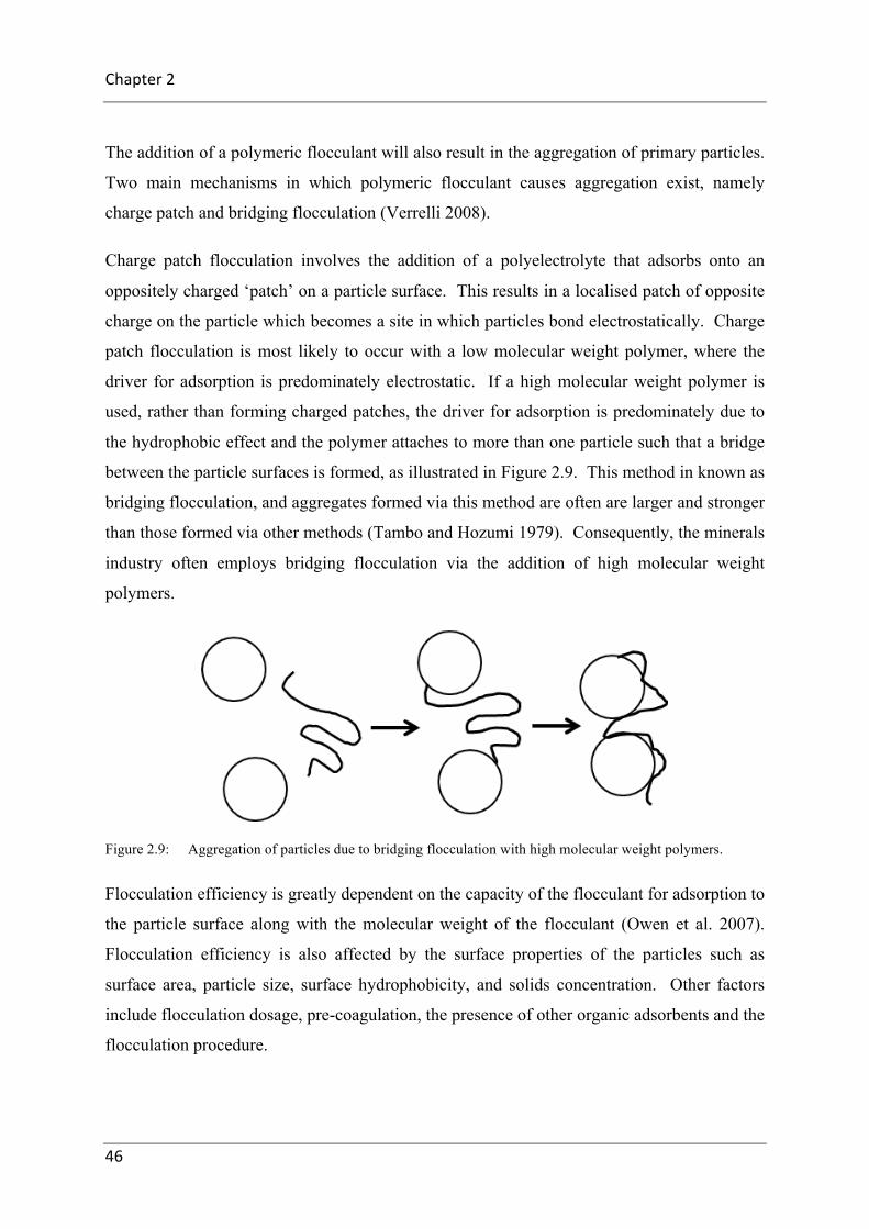
Chapter2

46

The addition of a polymeric flocculant will also result in the aggregation of primary particles.

Two main mechanisms in which polymeric flocculant causes aggregation exist, namely

charge patch and bridging flocculation (Verrelli 2008).

Charge patch flocculation involves the addition of a polyelectrolyte that adsorbs onto an

oppositely charged ‘patch’ on a particle surface. This results in a localised patch of opposite

charge on the particle which becomes a site in which particles bond electrostatically. Charge

patch flocculation is most likely to occur with a low molecular weight polymer, where the

driver for adsorption is predominately electrostatic. If a high molecular weight polymer is

used, rather than forming charged patches, the driver for adsorption is predominately due to

the hydrophobic effect and the polymer attaches to more than one particle such that a bridge

between the particle surfaces is formed, as illustrated in Figure 2.9. This method in known as

bridging flocculation, and aggregates formed via this method are often are larger and stronger

than those formed via other methods (Tambo and Hozumi 1979). Consequently, the minerals

industry often employs bridging flocculation via the addition of high molecular weight

polymers.

Figure 2.9: Aggregation of particles due to bridging flocculation with high molecular weight polymers.

Flocculation efficiency is greatly dependent on the capacity of the flocculant for adsorption to

the particle surface along with the molecular weight of the flocculant (Owen et al. 2007).

Flocculation efficiency is also affected by the surface properties of the particles such as

surface area, particle size, surface hydrophobicity, and solids concentration. Other factors

include flocculation dosage, pre-coagulation, the presence of other organic adsorbents and the

flocculation procedure.

Theory

47

2.6.3 Aggregate formation and structure

Extensive experimental and theoretical work has been reported in the area of aggregation

kinetics and the evolution of aggregate structures (Gregory 1987, Spicer et al. 1998, Biggs et

al. 2000, Heath et al. 2006, Runkana et al. 2006). During flocculation, aggregate growth can

be considered as a reaction pathway and separated into four main stages. (i) Dispersed, (ii)

Mixing and adsorption, (iii) Aggregation and (iv) Rupture (Gregory 1987).

i. The dispersed stage is pre-addition of flocculant and all solid particles are dispersed.

ii. During the mixing and adsorption stage, the polymer begins to adsorb to the particles

creating large porous aggregates with high settling rates. Dispersed particles still

exist and clarity is still low.

iii. In the aggregation stage, significant capture of particles occurs and aggregates start to

be eroded in size. This results in a slight decrease in settling rate and an increase in

clarity.

iv. Further mixing past the aggregation stage results in irreversible aggregate rupture

decreasing both clarity and settling rate.

The rate of the flocculation pathway is largely dependent on the particle-particle collision

frequency, the hydrodynamic conditions as well as the robustness to shear of the aggregate

structures (Gregory 1987, Krutzer et al. 1995).

The majority of research into the understanding of aggregate formation has been conducted to

further understand the relationship between flocculation conditions and aggregate structure.

The work shows that shear rate during flocculation greatly affects aggregate structure, size

and strength (Yeung et al. 1997, Swift et al. 2004). The relationship between aggregate

structure and dewatering behaviour is less well understood.

Initially, Tambo and Watanabe (1979) used Stokes velocity to describe the settling rate of an

aggregate. The difficulty here is that aggregates are porous and often fractal solid structures

(Mueller et al. 1966, Li et al. 1986, Li and Fanczarczyk 1988). The porous nature of the

aggregate structure, led Johnson et al. (1996) to use a permeability factor to predict the

sedimentation velocity based on aggregate size. As a consequence, Sutherland and Tan

Chapter2

48

(1970) treated the flow of liquid around and through the aggregates separately. Flow of

liquid around the aggregate was evaluated using Stokes law, while flow through the

aggregate was calculated using Darcy’s law (Darcy 1856). The Debye-Brinkman extension

of Darcy’s law was suggested (Neale et al. 1973), due to the uncertainty of applying Darcy’s

law to a highly porous material, such as a flocculated aggregate.

Gregory (1997) suggested that flocculated aggregates are fractal and hence their permeability

is dependent on not only their size, but also the radial distribution of mass. Using the idea of

a fractal aggregate, Chellam and Wiesner (1993), used the Carmen-Kozeny equation (Carman

1956) to predict the permeability of an aggregate. This worked showed that the aggregate

permeability is inversely related to its fractal dimension. Li and Logan (2001) showed that

the Carmen-Kozeny equation is not adequate for aggregates with low permeability and that

Brinkman and Happel correlations are better suited at predicting the scaling of aggregate

properties with fractal dimension.

Aggregate structures as a result of polymer bridging flocculation can be predicted with

reasonable accuracy for given flocculation conditions. Common methods employed include

the Monte Carlo method used by Dickinson and Euston (1991) and population balance

models (Heath and Koh 2003, Heath et al. 2006, Runkana et al. 2006).

Further work in relation to aggregation, agglomeration, flocculation and floc characterisation

can be found within the research by R. Amal. This includes but is not limited to Spicer et al.

(1998), Condie et al. (2001), Selomulya et al. (2003), Lee et al. (2003) and Selomulya et al.

(2004).

The literature pays scant attention to the effect of change in aggregate structure post

flocculation on the settling velocity. The interaction forces in the suspension will largely

influence the restructure of an aggregate post flocculation. The role of shear and

compression forces in modifying the aggregate structure is rarely considered.

2.7 Aggregate Densification

Application of dewatering theory and in particular equation 2.20 have been successful in

describing one dimensional dewatering on both a laboratory and industrial scale (Landman et

Theory

49

al. 1995, de Kretser et al. 2001). However, for gravity thickening, significant discrepancies

still exist between dewatering theory prediction and actual industrial data indicating a

limitation in the phenomenological models. These discrepancies have been accounted for in

gravity thickening through the use of an empirical correction factor known as the

permeability enhancement factor (Usher 2002). Typical enhancement factors range between

1 and 100 (Usher and Scales 2009).

As implied, the dewatering behaviour of aggregates is greatly dependant of the structure of

the aggregate and any structure change during dewatering can result in a change in the

dewatering behaviour. Raking within a thickener is the main contributor to aggregate

restructuring by imparting shear onto the aggregates (Usher et al. 2009). Other sources of

shear include aggregate-aggregate and aggregate-wall interactions. Experiments have shown

that the rate at which aggregates densify is related to the magnitude and time of shear(Kiviti-

Manor 2016). It has also been shown that a critical shear rate exists at which shear rates

above this value is detrimental to dewatering as aggregates start to erode, causing a decrease

in settling rate and permeability (Gladman et al. 2005).

Application of a shear force onto the aggregates is known to cause a structure change

whereby the aggregates densify and expel inter-aggregate liquid. This results in a decrease in

aggregate size and intra-aggregate permeability. However, the tortuosities around the

aggregates will decrease resulting in an overall increase in suspension permeability and as a

consequence, settling rate of the suspension (Mills et al. 1991, Farrow et al. 2000, Gladman et

al. 2005, Usher and Scales 2009). The main trends from experimental observations of

increased permeability due to shear are discussed below.

Modifications to the fundamental dewatering theory developed by Buscall and White (1987)

have been made to account for aggregate densification and the equations to be used within

this thesis are now outlined, the reader is referred to the literature for more detail (Gladman et

al. 2005, Usher et al. 2009, van Deventer et al. 2011, Grassia et al. 2014).

Chapter2

50

2.7.1 Experimental observations of aggregate densification

Many researchers (Farrow et al. 2000, Gladman 2006, Usher and Scales 2009, Gladman et al.

2010, van Deventer et al. 2011, Buratto et al. 2014, Spehar et al. 2015, Kiviti-Manor 2016)

have performed experiments to understand shear enhanced dewatering. Types of experiments

performed include; batch settling, Couette fluidisation and pilot scale thickening in a tall

column. Discussion of the experimental process and results for each type of experiment is

discussed below. For all experiments conducted, an increase in permeability was observed

due to the presence of shear. Measurements by Kiviti-Manor (2016) confirmed aggregate

size to decrease with shear while settling rate increased, implying aggregate densification as

the phenomena for shear enhanced dewatering.

2.7.1.1 Batch settling

van Deventer et al. (2011) performed raked batch settling tests to as a method of determining

the densification properties of a suspension. Raked batch settling tests resulted in a clear

dewatering enhancement, the suspension settling further and faster, compared to an

unsheared settling test. Application of aggregate densification theory provides a mechanism

of inferring a change in aggregate diameter through quantification of the enhancement in

permeability and compressibility. Further details regarding sheared batch settling analysis

are presented in section 2.7.5.

Batch settling tests with various means of imparting shear onto the aggregates, such as sloped

walls (Usher and Scales 2009) and curved surfaces such as vertical pickets or rods (Buratto et

al. 2014), have also been performed. Again, these experiments showed a clear dewatering

enhancement compared to a standard batch settling test, indicating shear enhanced

permeability and compression.

2.7.1.2 Couette fluidisation

A Couette shear rig was used by Gladman (2006) to investigate shear effects on flocculated

aggregates. This consisted of a Couette geometry in which the central cylinder was rotated in

order to apply shear to the aggregates within the annular region. The outer cylinder was

transparent such that aggregate restructure effects could be observed. However, due to the

Theory

51

high settling rates at the low solids concentrations required to distinguish individual

aggregates, such observations could not be made.

A constant suspension solids volume fraction can be obtained by off-setting gravity through

fluidisation. Adjustment of the fluidisation velocity allows for minimal aggregate

displacement. This allows restructuring effects to be observed. Kiviti-Manor (2016)

constructed and operated a fluidised Couette shear rig. The fluidised bed was sampled at

various fluidisation times and shear rates to quantify the change in aggregate diameter due to

Couette shear. Results indicated a significant decrease in aggregate size with shear rate,

fluidisation time and solids concentration. This decrease in aggregate size provides strong

evidence of aggregate densification due to shear.

Spehar (2014) applied novel techniques to quantify the extent of shear enhanced dewatering

within a Couette fluidisation rig. Due to a decrease in bed height and increase in fluidisation

velocity with fluidisation time, an increase in settling velocity was calculated. A hindered

settling function and subsequent aggregate diameter was inferred from the settling velocity.

Results indicate a decrease in aggregate diameter with increasing rotation rate, providing

evidence of aggregate densification due to shear.

2.7.1.3 Pilot scale tall column

A tall column (5 m high, 0.285 m internal diameter) was used by Gladman (2006), Spehar et

al. (2015) and Kiviti-Manor (2016) as a pilot scale thickener in order to quantify shear

induced dewatering. The tall column consisted of sampling ports every 20 cm along to allow

for sampling and determination of the solids concentration profile. This data allowed the

hindered settling function to be inferred along the column. Results indicate significant

performance enhancement was achieved when introducing shear through raking (Kiviti-

Manor 2016).

Spehar (2014) applied novel techniques to quantify the extent of shear enhanced dewatering

due to raking within a pilot scale thickener. Results indicate a reduction in aggregate

diameter of 14 % was achieved at moderate rake rotation rates.

Chapter2

52

2.7.2 Aggregate parameters

Aggregate densification is the change in aggregate size during dewatering due to shear and

collision processes. The theory and equations presented below were developed by Usher et

al. (2009) to describe aggregate densification. This theory assumes that the aggregates are

roughly spherical with an average diameter, dagg. The overall solids volume fraction within

the suspension is represented by φ, and defined as the total solids volume divided by the total

suspension volume. The average solids volume fraction within the aggregates is represented

by φagg, and defined as the total solids volume fraction within the aggregate divided by the

total aggregate volume. Furthermore, the aggregate volume fraction, ϕ, represents the

volume fraction of the suspension that the aggregates occupy such that;

. (2.57)

As aggregates densify, the aggregate diameter decreases while the solids fraction within the

aggregate, φagg, increases. Given that the solids concentration within an aggregate is

constant, performing a material balance results in;

, (2.58)

where φagg,0 and dagg,0 are the initial conditions before densification and Dagg is the scaled

diameter respect to the initial diameter. The density of the aggregate is therefore given by,

. (2.59)

Aggregate densification is a time dependant phenomenon, in which the aggregates diameter

follows an exponentially decaying trend under simple shear. In the absence of breakage,

there is a limit to the change in aggregate diameter than can be reached for a given applied

shear rate. This limit corresponds to a steady state diameter, Dagg,∞, in which further shear (at

the same level) will have no impact on the aggregate diameter. Dagg,∞, represents the

maximum possible extent of densification for a given system.

aggφφ

ϕ =

30,

3

30,

0,agg

agg

agg

aggaggagg Dd

d φφφ ==

( )aggliqaggsolagg φρφρρ −+= 1

Theory

53

The transient behaviour of aggregate densification has been characterised and the behaviour

has been shown to follow a simple linear first order differential equation;

, (2.60)

where A is a proportionality constant, or first order rate constant (s-1). In equation 2.60 the

rate and extent parameter have been assumed to be constant. More complex functions of

time, shear history and local solids concentration can be applied (van Deventer et al. 2011).

An analytical solution to 2.60 can be easily obtained via integration and application of the

necessary boundary conditions. Using the common boundary condition of initially un-

densified aggregates, (dagg = dagg, 0), integration of equation 2.60 results in,

. (2.61)

Other boundary conditions can arise due to pre-shearing of the aggregates. Figure 2.10

illustrates a typical aggregate diameter evolution when subject to shear. Also illustrated is

how the rate of change in aggregate diameter changes over time. As previously mentioned,

excessive shear will result in aggregate breakage and this has not been considered within this

theory.

( )∞−−= ,aggaggagg DDAdtdD

( ) ( ) ∞−

∞ +−= ,,1 aggAt

aggagg DeDtD

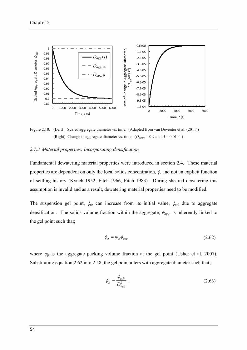
Chapter2

54

Figure 2.10: (Left) Scaled aggregate diameter vs. time. (Adapted from van Deventer et al. (2011))

(Right) Change in aggregate diameter vs. time. (Dagg∞ = 0.9 and A = 0.01 s-1)

2.7.3 Material properties: Incorporating densification

Fundamental dewatering material properties were introduced in section 2.4. These material

properties are dependent on only the local solids concentration, φ, and not an explicit function

of settling history (Kynch 1952, Fitch 1966, Fitch 1983). During sheared dewatering this

assumption is invalid and as a result, dewatering material properties need to be modified.

The suspension gel point, φg, can increase from its initial value, φg,0 due to aggregate

densification. The solids volume fraction within the aggregate, φagg, is inherently linked to

the gel point such that;

, (2.62)

where ϕp is the aggregate packing volume fraction at the gel point (Usher et al. 2007).

Substituting equation 2.62 into 2.58, the gel point alters with aggregate diameter such that;

. (2.63)

0.890.9

0.910.920.930.940.950.960.970.980.99

1

0 1000 2000 3000 4000 5000 6000

Scaled

AggregateDiameter,D

agg

Time,t(s)

Dagg

Dagginf

Dagg0

-1.E-04

-9.E-05

-8.E-05

-7.E-05

-6.E-05

-5.E-05

-4.E-05

-3.E-05

-2.E-05

-1.E-05

0.E+00

0 2000 4000 6000 8000

RateofC

hangeinAggregateDiameter,

dDagg/dt(s-1)

Time,t(s)

aggpg φϕφ =

30,

agg

gg D

φφ =

Dagg (t)

Dagg, ∞

Dagg, 0

Theory

55

This indicates a decrease in aggregate diameter, Dagg, causes the gel point to increase

(equation 2.63), and therefore a reduction in the compressive yield stress, Py(φ). At ϕ ≥ 1, the

aggregates are by definition, compressed. As the solids concentration further increases, the

material dewatering parameters revert to the undensified properties. Incorporating aggregate

densification, Py(φ) becomes:

, (2.64)

where Py,0 is the original undensified compressive yield stress, valid between the undensified

gel point, φg,0, and the close packing volume fraction, φcp, given by equations 2.24 to 2.26.

Py,1(φ) represents the densified compressive yield stress which is valid between the gel point,

φg, and the aggregate volume packing fraction, φagg. Py,1(φ) is defined such that it is zero at

the gel point and equal to Py,0(φ) at φagg. Figure 2.11 provides typical compressive yield

stress curves. For simplicity, it will also be assumed that the gradient, dPy/dφ is single valued

at φ = φagg, such that;

. (2.65)

The functional form for Py,1, will depend on the equation used to describe Py,0. As an

example, using equation 2.24 for Py,0 results in:

, (2.66)

where a1 and k1 are determined such that the gradient is smooth and continuous at φ = φagg

(equation 2.63), giving

, (2.67)

( )⎪⎩

⎪⎨

⎧

<≤

<≤

<

=

CPagg

aggg

g

y

yy forPPP

φφφ

φφφ

φφ

φ

0

1

0

( )( ) ( )( )aggyaggy PP φφ

φφ 0,1, ∂

∂=

∂

∂

1

)())((

),( 11,

k

g

gCPaggy

baDP

−

⎥⎥⎦

⎤

⎢⎢⎣

⎡

−

−+−=

φφ

φφφφφ

( )( )

( )( )( )( ) ( )20,

0,1

gagggCP

gagggaggaggCP

aggy

aggy

bb

PP

kφφφφ

φφφφφφ

φ

φ

−+−

−+−−⎟⎟⎠

⎞⎜⎜⎝

⎛ ʹ=

Chapter2

56

and

, (2.68)

where the gradient, P’y,0(φ) is calculated as

. (2.69)

Figure 2.11: Typical compressive yield stress curves, Py(φ,Dagg), at various extents of aggregate densification.

(Dagg = 1, 0.95, 0.90, 0.85) (Usher et al. 2009)

From fundamental dewatering theory (Buscall and White 1987), equation 2.32 can be

rearranged to obtain an expression for the settling velocity in terms of the hindered settling

function. As densification alters the aggregate structure, the fraction of fluid passing through

the aggregate decreases, while the fraction passing around increases. Hence in order to

account for aggregate densification, the settling velocity needs to be considered to have two

separate contributions, such that;

( )( ) ( )( )( )gaggaggCP

gaggk

aggy

bP

aφφφφ

φφφ

−+−

−=

− 110,

1

( )

( )( )( )

( )⎟⎟⎟⎟⎟⎟

⎠

⎞

⎜⎜⎜⎜⎜⎜

⎝

⎛

⎟⎟

⎠

⎞

⎜⎜

⎝

⎛

⎟⎟⎠

⎞⎜⎜⎝

⎛−

−

−−+

−

−+−−−

−

−

−=ʹ+1

0,

0,0,0

20,

0,0,

0,

0,

000, 0

1

1

k

g

gCPg

g

ggCP

g

gCP

y

ba

b

kaP

φφ

φφφφ

φφ

φφφφ

φφ

φφ

φ

1.E-03

1.E-02

1.E-01

1.E+00

1.E+01

1.E+02

0 0.2 0.4 0.6

Compressiv

eYieldStress,P

y(φ,D

agg)(kPa)


Dagg=1Dagg=0.95Dagg=0.90Dagg=0.85

Dagg = 1

Dagg = 0.95

Dagg = 0.90

Dagg = 0.85

Theory

57

, (2.70)

where u1 is from the flow of fluid around the aggregate and u2 is from the flow of fluid

through the aggregates. In order to obtain an expression for the flow of fluid around the

aggregates, u1, the aggregates are modelled as hard, spherical particles. Utilising equation

2.32 and the concept of an aggregate volume fraction, ϕ, an expression can be determined.

The flow of fluid through the aggregate, u2, is determined by the settling velocity at the solids

volume fraction within the aggregate, u(φagg), and normalised by the aggregate volume

fraction, ϕ. Combining and rearranging these two expression results an overall expression

for the settling velocity as a function of aggregate diameter (van Deventer et al. 2011),

, (2.71)

where u0 is the original undensified settling velocity given by,

. (2.72)

The change in the settling velocity components is illustrated in Figure 2.12. The following

expression for the hindered settling function incorporating densification is obtained from

equation 2.32,

, (2.73)

such that u(φ,Dagg) is determined via equation 2.71. Figure 2.12 (B) illustrates this behaviour.

( ) ( ) ( )tututu ,,, 21 φφφ +=

( ) ( ) ( )⎥⎥⎦

⎤

⎢⎢⎣

⎡−⎟⎟⎠

⎞⎜⎜⎝

⎛+=

agg

agg

agg

agg

agg

agg

agg

aggagg D

uD

uD

DDu

Du 0,030,

00,

330,

φφ

φ

φφφ

( )( )φφρ

φ0

2

01)(Rgu −Δ

=

( )( )agg

agg DugDR,1),(

2

φφρ

φ−Δ

=

Chapter2

58

Figure 2.12: (A) Variation in settling velocities with solids volume fraction where u1 is the flow around the

aggregates and u2 is the flow through the aggregates. Example given is for Dagg = 1 (Usher et al.

2009).

(B) Typical hindered settling function vs. solids volume fraction at different extents of aggregate

densification (Usher et al. 2009).

2.7.4 Modified Kynch method: Predicting settling curves with aggregate densification

The Kynch method, as outlined in sections 2.2 and 2.5.1.1, is a graphical method in which

iso-concentration lines are exploited to determine the flux density function. The settling

velocity and subsequently the hindered settling function can be determined from the flux

density function. The Kynch method, however assumes the settling velocity to be a function

of only the solids concentration and not a function of settling history (Kynch 1952, Fitch

1966, Fitch 1983).

A modified Kynch method has been developed by van Deventer et al. (2011) to determine the

hindered settling function, accounting for the effect of settling history through aggregate

densification. The modified Kynch method assumes shear to be the sole cause of any

dewatering enhancement observed, as compared to the standard settling test. An overview of

the modified Kynch method developed by van Deventer et al. (2011) is presented below.

1.E-07

1.E-06

1.E-05

1.E-04

1.E-03

1.E-02

1.E-01

0 0.1 0.2 0.3

SeplingVe

locity,u(φ)(ms-

1 )


u1Dagg1

u2Dagg1

utotDagg1

1.E+06

1.E+07

1.E+08

1.E+09

1.E+10

1.E+11

0 0.1 0.2 0.3 0.4R(φ,Dagg)(kgs-

1 m-2)


Dagg=1

Dagg=0.95

Dagg=0.90

Dagg=0.85

Dagg = 1

Dagg = 0.95

Dagg = 0.90

Dagg = 0.85

u1

u2

utotal

Theory

59

On a plot of height vs. time, the suspension interface height, h(t), comprises of three main

settling regions, namely the initial, fan and compression region. As discussed in section 2.2,

the possibility of additional regions and various settling modes can occur however the

modified Kynch method is valid for settling analogous to mode 3a type settling, typical of

most industrial settling problems (Lester et al. 2005). For mode 3a settling, there is a smooth

transition from the initial settling zone to the primary fan region without a discontinuity in the

solids concentration. For descriptions of other modes, the reader is directed to work by

Lester et al. (2005).

Analogous with Kynch analysis, the modified Kynch method is valid for all solids

concentrations up to a defined fan limit, φfl,0, determined using the condition given by Lester

et al. (2005),

0,0,

)(:)max(

gfl

ffφφφ

φφφ

−=

∂

∂= . (2.74)

A fan limit can be defined based on a densified gel point, however, the applicability of this

densified fan limit is not clear (van Deventer et al. 2011) and the undensified fan limit is

utilised as the maximum.

Within the fan region, iso-concentration lines, xφ(t), propagate upward from the base of the

settling cylinder, with a propagation velocity, dxφ/dt, related to the solids flux, given by,

( )φ

φφ

φ

φφ

∂

−∂=

∂

∂=

),(.),( aggagg DuDf

dt

dx, (2.75)

where the settling velocity accounting for densification is given by equation 2.71.

Determination of a rising iso-concentration line, xφ(t), is via integration of the propagation

velocity, equation 2.75, from time zero such that,

( )dt

Dutx

t

t

agg∫= ∂

−∂=

0

),(.)(

φ

φφφ . (2.76)

A construction line can also be evaluated such that,

Chapter2

60

∫=

−=t

taggcaggc dttDuhttDh

00, ))(,()),(,( φφ , (2.77)

where the initial height of the construction line, hc,0, is given by the mass balance,

φφ 00

0,h

hc = . (2.78)

For a given settling interface solids concentration, the intersection of the iso-concentration

line, equation 2.77, and the construction line, equation 2.78, such that,

)()),(,( txttDh aggc φφ = , (2.79)

provides a predicted height vs. time, h(ti) datum point. Solving for the intersections of the

iso-concentration lines, equations 2.76, and construction lines, equation 2.77, at a range of

solids concentrations up to the fan limit, φfl,0, provides a method by which settling interface

height vs. time function data within can be predicted for times greater than τ1 and solids

concentrations from φ* to φfl,0 (with φ* and τ1 defined below).

At early times, t < τ1, where the solids concentration at the settling interface is equal to the

initial solids concentration, φ0, the height of the interface with aggregate densification is

given by equation 2.77 evaluated at the initial solids concentration and initial settling height,

φ = φ0 and hc,0 = h0, such that h(t) = hc(φ0,Dagg(t),t). A transition arises at t = τ1, where the

interface solids concentration is no longer φ0 (Lester et al. 2005). This occurs when the

interface at the initial solids concentration intersects the iso-concentration line at the lowest

solids concentration present in the primary fan, φ*. This occurs at xφ*, given by:

)()),(,()( 1*1101 τττφτ φxDhh aggc == . (2.80)

This transition represents the end of the initial settling zone and the beginning of the fan

zone. At times greater than τ1, the solids concentration increases while settling velocity

decreases. Due to densification, a discontinuity in solids concentration may occur at the

Theory

61

transition between the initial settling zone and the start of the fan region. Hence the solids

concentration at the start of the fan zone, φ*, will be greater than or equal to the initial solids

concentration. The value of φ* for mode 3a settling is equal to the initial solids

concentration, therefore τ1 can be determined by solving for the intersections of the iso-

concentration line, equation 2.76, and construction line, equation 2.77, at the initial solids

concentration. For solution methods where φ* is greater than φ0, the reader is directed to

Lester et al. (2005).

2.7.5 Aggregate densification characterisation

In order to determine the rate and extent of aggregate densification for a given shear rate,

both raked and unraked settling tests are performed. The standard batch settling test provides

the undensified material properties, (R(φ), Py(φ), φg) through analysis methods outlined in

section 2.4. The equilibrium scaled aggregate diameter, Dagg,∞, is determined via equilibrium

bed height analysis similar to equilibrium batch settling analysis. The densification rate

parameter, A, is determined via optimisation methods utilising the modified Kynch method

described above.

Classical material property characterisation requires high solids data from pressure filtration

experiments. Densified material properties revert back to the undensified properties at φ >>

φagg, and hence sheared pressure filtration experiments are unnecessary.

The scaled equilibrium aggregate diameter, Dagg,∞, is determined via equilibrium analysis

similar to that performed on a standard settling test. Taking equation 2.46 and accounting for

densification gives,

. (2.81)

Given an assumed form that describes the behaviour of the compressive yield stress as a

function of aggregate densification, the equilibrium aggregate densification can be

determined. Dagg in equation 2.81 is determined via varying the densified gel point estimate

( ) ∫Δ

−

−

Δ=

0

10

),(11

φρρogh aggy

aggb dpDpPg

Dh

Chapter2

62

until the predicted bed height matches the bed height obtained experimentally. This value is

the final densification, defined as Dagg,∞.

The rate of aggregate densification is determined through optimisation. For given

densification parameters, Dagg,∞, and A, the modified Kynch method provides a prediction of

the suspension interface over time. Actual sheared batch settling data is compared to this

prediction, and the densification rate parameter is varied until an optimum fit is obtained.

The goodness of the fit of the predicted data versus the actual experimental data is quantified

though a mean square proportional error function, Ē,

, (2.82)

where texp is the experimental time taken to reach a certain height, tcalc is the time to reach the

same given height and n is the total number of data points fitted.

2.8 Modelling of Transient Batch Settling

This section covers the basic equations and theory used in compressional rheology with

specific applications to modelling transient batch settling. More comprehensive details can

be found in Landman and White (1994), de Kretser et al. (2003), Stickland and Buscall

(2009), Usher et al. (2009), Zhang et al. (2013) and Grassia et al. (2014).

Modern dewatering theory results in the following one dimensional conservation equation,

(as described in 2.2 – Modern Dewatering Theory);

. (2.83)

Given the correct application of boundary conditions, equation 2.83 can be used to predict

settling in many one-dimensional dewatering processes within a range of applications

(Auzerais et al. 1990, Howells et al. 1990, Bergstrom 1992, Burger and Concha 1998, Bustos

et al. 1999, Karl and Wells 1999, Diehl 2000, Bürger and Karlsen 2001). The solution

∑ ⎟⎟⎠

⎞⎜⎜⎝

⎛ −=

2

exp

exp1ttt

nE calc

( )⎥⎦

⎤⎢⎣

⎡ −Δ++

∂

∂

∂

∂=

∂

∂

)(1)()(

2

φφ

ρφφφ

φφ

Rgtq

zD

zt

Theory

63

methods used to predict transient batch settling is now outlined. Solution methods used to

predict thickener performance are outlined in section 2.9.

2.8.1 Finite discretisation

Based on background dewatering theory, transient batch settling can be predicted using an

upwind finite difference algorithm. The transient batch settling prediction algorithm employs

an semi-implicit finite difference method, based on the work of Burger et al. (2001). An

explicit scheme also exists, but this was converted into the semi-implicit scheme due to

computational time constraints (Spehar 2014). The theory and solution method for the semi-

implicit scheme, developed by Spehar (2014), is now presented. For details of the explicit

scheme or further information on the semi-implicit scheme, the reader is referred to (Spehar

2014)

Incorporation of the underlying dewatering material properties, Py(φ) and R(φ), into a single,

elegant differential equation results in the following one dimensional conservation equation

in which compression is irreversible;

, (2.84)

where f(φ) is the solids flux and D(φ) is the solids diffusivity defined by equations 2.15 and

2.36 respectively, and q(t) is the overall linear suspension flowrate in the z-coordinate

direction.

For the case of simple transient batch settling, the boundary condition where no net material

flows from the base to the top of the sedimentation column is

for all z; , (2.85)

where h0 is the initial height of the suspension. Applying this boundary condition, simplifies

equation 2.84 to:

⎟⎠

⎞⎜⎝

⎛∂

∂

∂

∂=+

∂

∂+

∂

∂

zD

zftq

ztφ

φφφφ )())()((

0)( =tq ],0[ 0hz∈

Chapter2

64

, (2.86)

where AD(φ) is an integrated diffusion coefficient of D(φ) such that

. (2.87)

The solids volume fraction over J evenly distributed, discrete height elements, , is

determined in n increments of time, t, over time steps, Δt. For the initial condition, where n =

0 and t = 0, the solids volume fraction of each height element is set at the initial solids

volume fraction such that, for all j from 1 to J.

The values of for are defined by the following implicit finite difference

discretisation of the governing differential equation,

(2.88)

where is the Engquist-Osher flux function scheme (Engquist and Osher 1981)

defined by,

. (2.89)

A number of intermediate functions are determined via,

, , (2.90)

where the slopes are

)()(2

2φ

φφDAzz

ft ∂

∂=

∂∂

+∂∂

∫=φ

φφφ0

)()( dDAD

njφ

,00 φφ =j

,1+njφ ,,..., 12 −= Jj

( ) ( )( )

,)()()()(1

,,1

11

,,1

,1

,1

⎟⎟⎠

⎞⎜⎜⎝

⎛

Δ

−−

Δ

−

Δ=

−Δ

+Δ

−

−+

−+

+

xAA

xAA

x

ffxt

njD

njD

njD

njD

Lnj

Rnj

EOLnj

Rnj

EOnj

nj

φφφφ

φφφφφφ

( )⋅⋅,EOf

( ) ∫ ∫++=u v

EO dssfdssffvuf0 0

)}(',0min{)}(',0max{)0(,

2,

njn

jLn

j

κφφ −=

2,

njn

jRn

j

κφφ +=

Theory

65

, (2.91)

and the min-mod limiter function, MM(a,b,c) is given by

( )otherwise

0,, if0,, if

0

},,max{},,min{

,, ≤

>

⎪⎩

⎪⎨

⎧

= cbacba

cbacba

cbaMM . (2.92)

The min-mod limiter function requires the following boundary conditions due to no flow at

the ends of the column such that;

. (2.93)

With no flow of solids (or fluid) at the upper or lower boundary of the column, the following

boundary conditions apply:

, (2.94)

and

. (2.95)

The solids concentrations for all subsequent times are determined by application of the above

equations, for incremented values of n, until sedimentation and consolidation effectively

ceases. Solving the above equations is achieved through matrix methods as outlined by

Spehar (2014).

Initially, n = 0 (t = 0), the solids volume fraction at all height elements is set to the initial

solids concentration, φj0 = φ0 for all j from 1 to J. The maximum stable time step, Δt, is given

by;

⎟⎟⎠

⎞⎜⎜⎝

⎛−

−−= +

−+−

nj

nj

nj

njn

jnj

nj MM φφ

φφφφκ 1

111 ,

2,

01 == nJ

n κκ

( )( ) ⎟⎟⎠

⎞⎜⎜⎝

⎛

Δ−

Δ=

Δ+

ΔΔ

xAA

xf

xt

nD

nDLnRnEO

n )()(1,1 12,2

,1

1 φφφφ

φ

( )( ) ⎟⎟⎠

⎞⎜⎜⎝

⎛

Δ−

−Δ

=−Δ

+ΔΔ −

− xAA

xf

xt

nJD

nJDLn

JRn

JEO

nJ )()(1,1 1,,

1φφ

φφφ

Chapter2

66

, (2.96)

where ε is the safety factor and φmax is the maximum potential solids volume fraction

anywhere within the suspension given by,

. (2.97)

In solving equations 2.84 to2.97, a solids concentration profile within the settling column is

calculated at incremental n, (or time steps, Δt) until sedimentation and consolidation ends.

2.8.2 Implicit scheme

For a single settling test at reasonable accuracy, J = 100, on a standard desktop computer, the

semi-implicit scheme without densification has a computational time of order 2-4 hours.

Incorporation of aggregate densification increased the simulation time by an order of

magnitude (depending on accuracy). The computational time was further increased to

approximately 60 to 120 hours using the required accuracy. Given the method proposed in

Chapter 4 to analyse experimental batch settling data, an implicit scheme was developed to

overcome the issue of the vastly slower computational times.

Berres et al. (2005) developed an implicit scheme that predicts the transient dewatering

behaviour of a particulate suspension within a centrifuge. The application of this method to

transient batch settling is outlined below. The implicit scheme utilises the finite discretisation

equations 2.84 to 2.95, however a different solution method. The solution method is outlined

below.

For the implicit scheme, further manipulation of equation 2.88 is achieved by performing

Taylor expansions on the flux and diffusion terms followed by rearrangement into the form:

, (2.98)

which can be put into a diagonal matrix of the form , where

( )( )( )φε

φφfMax

xt

ʹ−Δ

=Δ≤< max0

312

( ) 00hgP Maxy φρφ Δ=

jnjj

njj

njj

njj

njj Bedcba =Δ+Δ+Δ+Δ+Δ ++−− 2112 φφφφφ

BA =Δφ̂

Theory

67

. (2.99)

The matrix A is a diagonal matrix made up of the following components;

, (2.100)

, (2.101)

, (2.102)

, (2.103)

and

. (2.104)

The terms in matrix B are defined as

. (2.105)

⎟⎟⎟⎟⎟⎟⎟⎟⎟

⎠

⎞

⎜⎜⎜⎜⎜⎜⎜⎜⎜

⎝

⎛

=

⎟⎟⎟⎟⎟⎟⎟⎟⎟⎟

⎠

⎞

⎜⎜⎜⎜⎜⎜⎜⎜⎜⎜

⎝

⎛

−

−

−

−

−

⎟⎟⎟⎟⎟⎟⎟⎟⎟⎟

⎠

⎞

⎜⎜⎜⎜⎜⎜⎜⎜⎜⎜

⎝

⎛

−

+−

+−

+

+

+

−−−−

J

J

j

nJ

nJ

nJ

nJ

nj

nj

nn

nn

JJJ

JJJJ

jjjjj

BB

B

BB

cbadcba

edcba

edcbedc

1

2

1

11

11

1

21

2

11

1

1111

2222

111

0

0

!

!

!

!

"#

$$$$$!

!$$$$$#

"

φφ

φφ

φφ

φφ

φφ

( )nj

Lnj

Rnj

EO

j

fx

a2

,,1 ,1

−

−

∂

∂

Δ−=

φ

φφ

( ) ( )nj

Dnj

Lnj

Rnj

EO

nj

Lnj

Rnj

EO

jA

xf

xf

xb

11

,,1

1

,1

, 1,1,1

−−

−

−

+

∂

∂

Δ−

∂

∂

Δ−

∂

∂

Δ=

φφ

φφ

φ

φφ

( ) ( )nj

Dnj

Lnj

Rnj

EO

nj

Lnj

Rnj

EO

jA

xf

xf

xtc

φφ

φφ

φ

φφ

∂∂

Δ+

∂

∂

Δ−

∂

∂

Δ+

Δ= −+ 2,1,11 ,,

1,1

,

( ) ( )nj

Dnj

Lnj

Rnj

EO

nj

Lnj

Rnj

EO

jA

xf

xf

xd

11

,,1

1

,1

, 1,1,1

++

−

+

+

∂∂

Δ−

∂

∂

Δ−

∂

∂

Δ=

φφ

φφ

φ

φφ

( )nj

Lnj

Rnj

EO

j

fx

e2

,1

, ,1

+

+

∂

∂

Δ=

φ

φφ

( ) ( ) ⎟⎟⎠

⎞⎜⎜⎝

⎛

Δ

+−+−

Δ= −+

+− xAAA

ffx

BnjD

njD

njDLn

jRn

jEOLn

jRn

jEO

j

)()(2)(,,1 11,

1,,,

1

φφφφφφφ

Chapter2

68

The solids concentrations for all subsequent times are determined by solution of the tri-

diagonal matrix, for incremented values of n, until sedimentation and consolidation

effectively ceases.

2.8.3 Accounting for aggregate densification

Current implementation of both the explicit and semi-implicit schemes account for aggregate

densification through recalculation of the material dewatering properties at each time step

(Spehar 2014). This is a crude method of incorporating aggregate densification but it has

been shown to be adequate for the purposes required and employing this method and it is

feasible to turn on or off aggregate densification at any time step. This provides the

possibility of predicting settling behaviour where shearing/raking was not present over the

entirety of the settling test, for example, if raking either ceases before complete settling or

starts at times greater the t = 0. Further possibilities include changing the rate or extent of

aggregate densification at any time step, allowing for aggregate densification parameters to

be more complex functions of for instance, solids concentration.

Incorporation of a delayed raking start time, tstart, and raking stop time, tstop, were included

into the equation describing the change in aggregate diameter with time, Dagg(t) (equation

2.60). This resulted in;

, (2.106)

where Dagg,0 is the initial scaled aggregate diameter (most often Dagg,0 = 1). Equation 2.106

has been implemented within the Transient Batch Settling algorithm through recalculation of

aggregate properties at every time step. Figure 2.13 depicts the effect of tstart and tstop on the

reduction in aggregate diameter over time.

( ) ( ) ( )

( ) ( )stop

stopstart

start

aggttA

aggagg

aggttA

aggagg

agg

agg

ttttt

tt

DeDDDeDD

DtD

startstop

start

>

≤<

≤

⎪⎩

⎪⎨

⎧

+−

+−=

∞−−

∞

∞−−

∞

,,0,

,,0,

0,

Theory

69

Figure 2.13: Scaled aggregate diameter as a function of time, Dagg(t), as described by equation 2.106 using

parameters: A = 0.01 s-1, Dagg,∞ = 0.9, tstart = 100 s and tstop = 300 s.

2.9 Thickener Modelling

This section covers the basic equations and theory used in compressional rheology with

specific applications to modelling steady state thickener performance. More comprehensive

details can be found in (Landman and White 1994, de Kretser et al. 2003, Usher and Scales

2005, Stickland and Buscall 2009, Usher et al. 2009, Zhang et al. 2013, Grassia et al. 2014).

Modern dewatering theory elegantly describes dewatering through a simple one-dimensional

conservation equation, equation2.20. The solution methods used to predict steady state

thickening is now outlined. Transient thickener prediction is considered outside of the scope

of this thesis however for information on transient thickener prediction and further

information on steady state thickening, the reader is referred to Burger et al. (2001), Usher

and Scales (2005), Usher et al. (2009) and Spehar (2014).

0.9

0.92

0.94

0.96

0.98

1

0 100 200 300 400

Sca

led

Agg

rega

te D

iam

eter

, Dag

g

Time, t (s)

Standard Modified Raking

tstart = 100 s tstop = 300 s

Chapter2

70

2.9.1 1D steady state thickener modelling

Numerous authors have combined the theory of free settling and compression in order to

produce a one-dimensional steady state thickener (1D SST) model that predicts thickener

operation from fundamental material properties (Usher and Scales 2005, Bürger and Narváez

2007, Usher et al. 2009, Zhang et al. 2013, Grassia et al. 2014).

An algorithm was developed by Usher and Scales (2005) in which one dimensional steady

state thickener operation could be predicted from fundamental material properties. This

model provided thickener throughput as a function of underflow concentration. It was then

adapted (Usher et al. 2009) to account for the extent of aggregate densification through

incorporation of the dependency on aggregate diameter into the fundamental dewatering

properties. The theory and algorithms behind these models are outlined below. The reader is

referred to the work of Usher and Scales (2005) and Usher et al. (2009) for further details.

Both of these 1D-SST models involve the determination of the solids throughput versus

underflow concentration in two parts, sedimentation, and consolidation. The limiting flux

within the sedimentation zone is determined via the simple Coe and Clevenger (1916)

method. Predicting the consolidation component requires taking bed compression into

account and is solved through integration of a differential equation developed from the

fundamental dewatering theory. The overall limiting solids flux at a given underflow

concentration and bed height is simply the minimum of the two predicted fluxes. Example

predictions of operating fluxes are illustrated in Figure 2.14.

Theory

71

Figure 2.14: Steady state thickener performance predictions of solids flux, q, vs. underflow solids

concentration, φu, for a range of extents of aggregate densification and a bed height of 1 m.

(Usher and Scales 2005, Usher et al. 2009)

2.9.2 Sedimentation theory

Rearrangement of equation 2.32, provides the following expression for the free settling

velocity of particles undergoing sedimentation:

( ))(

1)(2

φφρ

φRgu −Δ

= . (2.107)

The traditional Coe and Clevenger method suggests that this settling rate be used in a

material balance to determine the thickener steady state solids flux (for the maximum

thickener cross sectional area), q, for suspension at any solids concentration, φ, and for a

given underflow solids concentration, φu (Fitch 1966);

1.E-07

1.E-06

1.E-05

1.E-04

1.E-03

0 0.1 0.2 0.3

SolidsF

lux,q(m

s-1 )

UnderflowSolidsConcentranon,φu(v/v)

Dagg=1

Dagg=0.95

Dagg=0.90

Dagg = 1

Dagg = 0.95

Dagg = 0.90

φ0

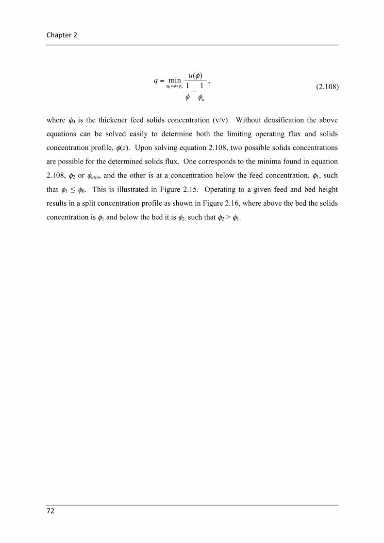
Chapter2

72

, (2.108)

where φ0 is the thickener feed solids concentration (v/v). Without densification the above

equations can be solved easily to determine both the limiting operating flux and solids

concentration profile, φ(z). Upon solving equation 2.108, two possible solids concentrations

are possible for the determined solids flux. One corresponds to the minima found in equation

2.108, φ2 or φmin, and the other is at a concentration below the feed concentration, φ1, such

that φ1 ≤ φ0. This is illustrated in Figure 2.15. Operating to a given feed and bed height

results in a split concentration profile as shown in Figure 2.16, where above the bed the solids

concentration is φ1 and below the bed it is φ2, such that φ2 > φ1.

u

uqu

φφ

φφφφ 11

)(min0

−=

>>

Theory

73

Figure 2.15: Solids flux, q (m s-1) calculated via material balance (equation 2.108) at a range of solids

concentration, φ (v/v), for a permeability-limited thickener without densification. Typical mineral

suspension material properties and an operating underflow concentration, φu, of 0.1 v/v were used.

The local minima, q = 3.5x10-5 m s-1, provides the maximum operating solids flux, qop. At qop,

two potential solids concentrations are possible, φ1 and φ2, which represent the solids

concentration profile.

1.E-05

1.E-04

1.E-03

0 0.02 0.04 0.06 0.08 0.1

SolidsF

lux,q(m

s-1 )


φu

qop φ1 φ2

Chapter2

74

Figure 2.16: Example solids concentration profile, z(φ), for a permeability limited thickener without

densification operating at an underflow solids concentration and solids flux of φu = 0.1 v/v and qop

= 3.5 x10-5 m s-1. A feed and bed height of 5 and 1 m were used. Solids concentrations, φ1 and

φ2, were determined via equation 2.108 (illustrated in Figure 2.15).

During aggregate densification, the fundamental material properties become a function of

local solids concentration, φ, as well as time, t. Incorporating this into equations 2.107 and

2.108 results in:

, (2.109)

and;

0

1

2

3

4

5

0 0.02 0.04 0.06 0.08 0.1

Height,z(m

)

SolidsConcentration,φ(v/v)

( ) ( )( )tRgtu,1,

2

φφρ

φ−Δ

=

φ0

φu

φ1 φ2

Theory

75

. (2.110)

Usher et al. (2009) solved equations 2.109 and 2.110 by assuming time independent material

properties, and that the aggregates have a specified aggregate diameter limit defined as,

Dagg,∞. The resultant 1D SST model provides boundaries of what can be achieved through

incorporation of aggregate densification, despite the assumption of time independent

properties being unrealistic. The limiting flux can be easily solved via the same method as

without densification. An example result is shown in Figure 2.17 and Figure 2.18.

Figure 2.17: Example solids flux, q (m s-1) vs. solids concentration, φ (v/v), for a given underflow solids

concentration, φu (v/v) at varying extents of densification. Solving equation 2.81 results in

operating fluxes of 3.8x10-5, 5.6x10-5 and 9x10-5 m s-1 for Dagg = 1, 0.95 and 0.90 respectively

(shown by horizontal dashed lines). Note that this result assumes time independent material

properties.

u

tuqu

φφ

φφφφ 11

),(min0

−=

>>

1.E-05

1.E-04

1.E-03

0 0.02 0.04 0.06 0.08 0.1

SolidsF

lux,q(m

s-1 )


Dagg=1

Dagg=0.95

Dagg=0.90

φu

Dagg = 1

Dagg = 0.95

Dagg = 0.90

Chapter2

76

Figure 2.18: Example of a solids concentration profile, z(φ), for a thickener operated within permeability

limitations at a range of densification extents. For this example a feed and bed height of 5 and 1m

were used along with an underflow concentration of 0.1 v/v. Note that each solids concentration

profile is at a different operating flux and that this result assumes time independent material

properties.

2.9.3 Consolidation theory

It is possible that the operational flux predicted via sedimentation is unachievable due to the

compressibility of the suspension. Consolidation often results is a much lower achievable

solids flux for a given underflow concentration. Consolidation occurs when the solids

concentration within the thickener is greater than the gel point, φ > φg. In order to account for

consolidation, the compressive yield stress must be considered in the force balance equation

(along with buoyancy and drag forces) such that;

. (2.111)

Rearrangement of equation 2.111 gives;

0

1

2

3

4

5

0 0.02 0.04 0.06 0.08 0.1

Height,z(m

)


Dagg=1

Dagg=0.95

Dagg=0.90

φ0

( )( )

( )01

1 2 =Δ−−⎟⎟⎠

⎞⎜⎜⎝

⎛−

−φρ

φφ

φ

φφ

φφ g

dzd

ddP

qR y

u

φu

Dagg = 1

Dagg = 0.95

Dagg = 0.90

Theory

77

.

(2.112)

Solving equation 2.112 for a given solids flux, q, and underflow solids concentration, φu,

along with the appropriate boundary conditions will result in the determination of the solids

concentration profile within the thickener, φ(z). Inverting equation 2.112 relates the change

in height with solids concentration and has been shown to provide improved computational

speed (Usher and Scales 2005). The addition of a thickener shape factor, α(z) allows for any

variations in cross sectional area in the thickener to be taken into account (Usher and Scales

2005). The resultant differential equation to solve is;

, (2.113)

where α(z) is defined as

, (2.114)

where dt is the thickener diameter (m). Given the top of the bed, hb, is at the gel point, φg,

and the bottom is at the underflow concentration, φu, the following boundary conditions,

, (2.115)

and

, (2.116)

( )( )

( )φ

φ

φρφφ

φφ

φ

ddP

gqR

dzd

y

u

Δ−⎟⎟⎠

⎞⎜⎜⎝

⎛−

−=

11 2

( )

( )( ) ( )

φραφ

φφφ

φφ

φg

zqRd

dP

ddz

u

y

Δ−⎟⎟⎠

⎞⎜⎜⎝

⎛⎟⎟⎠

⎞⎜⎜⎝

⎛−

−

=

11 2

( ) ( )2

max,⎟⎟⎠

⎞⎜⎜⎝

⎛=

t

t

dzdzα

( ) 0=uz φ

( ) bg hz =φ

Chapter2

78

can be applied to determine the solids concentration profile within the bed for a given solids

flux, q, and underflow concentration, φu. Equation 2.113 is solved for a given underflow

concentration, φu, via iterating on the solids flux, q, until equation 2.116 is satisfied. Iteration

is possible as the solids flux is bounded between zero and the solids flux obtained in the

sedimentation solution. As an addition, the solids residence time within the bed can be

calculated given,

. (2.117)

Again, Usher et al. (2009) solved for the limiting flux during consolidation equations 2.111 to

2.117 by assuming time independent material properties and that the aggregates have a

specified aggregate diameter limit, Dagg. This assumption removes the time dependency

within the equations and hence can be solved in the same method as for without densification.

An example thickener performance prediction result is shown in Figure 2.14.

2.9.4 Solids residence time

The above methods for determination of the steady state solids flux as a function of

underflow solids concentration assume that the permeability and compressibility of the

suspension does not alter with solids residence time. Aggregate densification is a dynamic

process in which the diameter of the aggregate is reduced with solids residence time

according to equation 2.60. Subsequently the permeability and compressibility of the

suspension also change with solids residence time, equations 2.66 and 2.73.

Other models have modified the above one-dimensional steady state thickening theory in

order to account for dynamic densification and in turn dynamic material properties. Zhang et

al. (2013) developed a model in which the thickener feed was at the initial solids gel point,

φg,0, and hence only consolidation was considered. Grassia et al. (2014) developed a model

to calculate the free settling limiting flux, ignoring any compression. These models however

do not combine the theory of sedimentation and consolidation to provide an overall limiting

flux. Combining these two is not as straight forward as the previous method, and hence this

is the focus of the work presented in Chapter 3.

( )qz

dzdt φ=

Theory

79

2.9.5 Entropy condition

As solutions to equation 2.20 are in general discontinuous, Bürger and Narváez (2007)

utilised the entropy condition (or selection criterion) by (Kružkov 1970) to select physically

relevant solutions. This entropy condition permits solids concentration profiles produced by

vanishing hydrodynamic diffusion. For application to steady state thickener modelling, this

entropy condition implies the solids concentration must increase down the thickener. Further

details on the entropy condition and derivation, which is beyond the scope of this paper, refer

to Kružkov (1970), Bürger et al. (2005) and Bürger and Narváez (2007).

Steady state modelling by Usher and Scales (2005), Usher et al. (2009), Zhang et al. (2013)

and Grassia et al. (2014) do not directly calculate the entropy condition due to difference in

methods, however it is believed that such condition has been satisfied. Modelling methods

within this thesis are based on those by Usher and Scales (2005), Zhang et al. (2013) and

Grassia et al. (2014) and therefore the entropy condition is not calculated however believed to

be satisfied. Further work involving the calculation of the entropy condition is recommended

however outside the scope of this thesis.

Chapter2

80

81

Chapter 3. THICKENER MODELLING

Chapter 3

Thickener Modelling

This chapter outlines the theory developed to account for the time dependent nature of

aggregate densification within a one-dimensional steady state thickener (1D SST) model.

Using this theory along with material properties representative of industrial mineral slurries,

predictions of steady state thickener performance have been produced. The effects of

operational variables, such as thickener feed rate, concentration, bed height and aggregate

densification parameters, on thickener performance have been investigated. Model

development was aimed at providing a relatively simplistic, fast, and easy to use model to aid

in both thickener operation and design.

3.1 Background Theory

A one dimensional steady state thickening model that looks to incorporate the effects of shear

induced aggregate densification (both rate and extent) has been developed. Previous work

has shown that the bounds of thickening can be predicted (the expected maximum and

minimum performance points) based on laboratory and pilot column testing to extract

material properties, but a knowledge of the dynamics between these bounds has not been

available.

A one dimensional steady state thickening model was developed by Usher and Scales (2005)

but without shear induced aggregate densification effects. This was upgraded to incorporate

Chapter3

82

the extent of aggregate densification (Usher et al. 2009) and current development takes the

next step to incorporate the rate of shear induced aggregate densification. This model

combines the theories of; sedimentation, suspension bed consolidation and aggregate

densification. Other workers have looked at the sedimentation and consolidation problems in

isolation but the difficult task of linking the two together is the next step (Zhang et al. 2013,

Grassia et al. 2014). This model uses material dewatering properties and thickener

operational parameters as inputs to produce steady state solids flux predictions for a range of

underflow solids concentrations.

Prediction of the solids throughput as a function of underflow solids concentration is

calculated in two parts. The first part considers sedimentation limited settling, previously

referred to as the permeability limit (Usher and Scales 2005), while the second considers

consolidation and compression of the suspension bed. The sedimentation limited settling and

compression calculations are combined to predict the steady state solids flux for each

underflow solids concentration.

It is important to note that in all the following equations, the solids flux, q, is defined as the

volume of solids per unit time per thickener cross sectional area, with SI units of m s-1.

However, to adhere to industry conventions, all graphs of solids flux are presented in tonnes

of solids per hour per square meter, where solids throughput in tonnes of solids per hour is

simply the solids flux multiplied by the cross-sectional area of the thickener. In all the

following equations and discussions, t is the solids residence time, while tres is the overall

solids residence time such that t(z = 0) = tres.

3.2 Model Assumptions and limitations

As with all models, there are a number of assumptions and limitations, which should be kept

in mind when utilising the model output. The assumptions and limitations of the model

presented within this chapter are:

• The model is one-dimensional

The model does not account for short circuiting and mixing and all dewatering

occurs in the vertical direction, with no horizontal flow of liquor or solids. Mixing

ThickenerModelling

83

and short-circuiting within a thickener is expected to be present, however minimal

providing efficient operation. Converting to a three-dimensional model to account

for dewatering in all directions significantly increases the complexity moving away

from the aim of producing a simplistic, fast and easy to use model.

• Line settling

This implies that the settling rate and permeability are functions of solids volume

fraction and all solid particles at the same height, settle at the same rate, with no

size segregation.

• Wall effects are negligible

This model assumes the thickener diameter is sufficiently large compared to the

suspension bed height such that any material hold up through wall effects can be

neglected.

• All aggregates produced during flocculation are equal

This implies that all aggregates settle at the same rate and have the same aggregate

densification properties.

• No solids exit via the overflow

• Steady state operation

• The thickener is straight walled

This model does not account for the cross sectional effects of a converging base

thickener

• Shear enhanced dewatering is accounted for through Aggregate Densification

All dewatering enhancement is assumed to be caused by aggregate densification

and described via equations presented within section 2.6.

• Equal distribution of shear

Along with the assumption of line settling, this also implies that all aggregates at

the same height are exposed to the same shear rate and for the same length of time.

• Aggregates do not break with excessive shear

In reality this is not the case, however the incorporation of aggregate breakage into

aggregate densification theory is yet to be performed. Hence for simplicity the

limitation of no breakage has been applied.

Chapter3

84

3.3 Model Inputs

The inputs required for the steady state thickener model include:

• Compressive yield stress, Py(φ), curve fit

• Hindered settling function, R(φ), curve fit

• Solid and liquor densities, ρsol and ρliq.

• Aggregate densification parameters, A and Dagg,∞

• Thickener feed and bed heights, hf and hb

• Feed solids concentration, φ0

All model results presented within this chapter utilise the following parameter values and

material property curve fits as model inputs.

3.3.1 Material properties

Functional forms and parameter values for undensified Py,0(φ) and R0(φ) properties have been

chosen such that they represent a typical flocculated industrial mineral slurry produced in the

feedwells of large scale gravity thickeners. Typical aggregate densification parameters,

A = 10-4 s-1 and Dagg,∞ = 0.8, shown by experiments in Chapter 4, have been used to describe

material aggregate densification behaviour.

The initial un-densified hindered settling function, R0(φ) = R(φ, Dagg = 1) is chosen here as

that described by equation 2.34. The values of the functional parameters are as used by

Usher and co-workers (Usher and Scales 2005, van Deventer et al. 2011), where ra, rg, rn and

rb are 5 x 1012, 0.05, 5 and 0, respectively. Additionally, the liquid is assumed to be water,

with a viscosity of η = 0.001 Pa s and density ρliq = 1000 kg m-3. The solid density is

assumed to be ρsol = 3200 kg m-3. The change in the hindered settling function with

densification is described by equation 2.73. The functional form for undensified, Dagg = 1,

and fully densified, Dagg = Dagg,∞ = 0.8, hindered settling function is shown in Figure 3.1.

In this model case study, the network strength is defined by the constitutive compressive

yield stress function shown in equations 2.24, 2.64 and 2.66. Functional parameters for

ThickenerModelling

85

equation 2.24, a0, b and k0, have chosen values of 0.9, 0.002 and 11, respectively as used by

Usher et al. (2009) and van Deventer et al. (2011).

The close packing volume fraction is the maximum possible solids concentration achievable,

and is assumed to be φcp = 0.8 for a polydisperse system. The initial gel point and aggregate

packing volume fraction are φg,0 = 0.1 and ϕp = 0.6 respectively. The value of φg,0 chosen

influences the solids concentration at which consolidation within the thickener needs to be

taken into consideration. The compressive yield stress function described by these equations

and parameters is shown in Figure 3.1.

Figure 3.1: Undensified (Dagg = 1) and fully densified (Dagg = Dagg,∞ = 0.8) hindered settling function, R(φ,t),

and compressive yield stress function, Py(φ,t), used in the model case study to predict thickener

throughput, q, as a function of underflow solids concentrations, φu. The hindered settling function

is governed by equations 2.34 and 2.73 with parameter values ra = 5 x 1012, rg = -0.05 and

rn = 5. The compressive yield stress functional form is governed by equations 2.24, 2.64 and 2.66

with parameter values a0 = 0.9, b = 0.002 and k0 = 11.

The shear yield stress is not utilised by this model, however it provides insight in determining

if the output suspension can be raked or pumped. The relation between τy(φ) and Py(φ) is

given by equation 2.27. For this case study, a scalar ratio of α = 20 will be used. The solids

flux function has been calculated for the model material properties at no densification, Dagg =

1, and full densification, Dagg = Dagg,∞ = 0.8, as shown in Figure 3.2.

1.E+06

1.E+07

1.E+08

1.E+09

1.E+10

1.E+11

0 0.1 0.2 0.3 0.4

Hin

dere

d S

ettli

ng F

unct

ion,

R(φ)

(Pa

s m

-2)

Solids Volume Fraction, φ (v/v)

R0RinfGelPoint

0.01

0.1

1

10

100

0 0.1 0.2 0.3 0.4 Com

pres

sive

Yie

ld S

tress

, Py(φ)

(k

Pa)


PyPy1

Py(φ)

Py(φ,Dagg,∞)

R(φ,Dagg =1)

R(φ,Dagg,∞)

φg

Chapter3

86

Figure 3.2: Undensified (Dagg = 1) and fully densified (Dagg = Dagg,∞ = 0.8) solids flux, f(φ,t) vs. solids

concentration, φ, where f(φ,t) = φ.u(φ,t).

3.3.2 Operating conditions

A thickener feed height of 5 m, a bed height of 2 m and a feed solids concentration of

0.05 v/v have been used, representing typical values seen within industry. Previous models

(Usher and Scales 2005) include a factor to account for change in cross sectional area but for

the purposes of the model here, the thickener will be assumed to be straight walled with no

cross sectional area variation (α(z) = 1).

3.3.3 Solids flux boundaries

The model by Usher et al. (2009) predicts the solids flux, q, for a range of underflow solids

concentrations, φu, for time independent material properties, Dagg = constant. The theory for

this model can be found in section 2.9.1. Application of this model for no densification,

0.E+00

2.E-05

4.E-05

6.E-05

8.E-05

1.E-04

1.E-04

1.E-04

0 0.05 0.1 0.15 0.2 0.25 0.3 0.35 0.4

SolidsF

lux,f(φ)(m

s-1 )


q_Dagginf

f0

Dagg = Dagg,∞ = 0.8

Dagg = 1

ThickenerModelling

87

Dagg = 1, and full densification, Dagg = Dagg,∞,provides lower and upper limits in solids flux

for each underflow solids concentration.

Aggregate densification is a dynamic process and the real solids flux will lie within these

limits. Dagg is sensitive to the overall solids residence time, tres, and the rate of aggregate

densification and therefore it is expected that q will be close to an un-densified value when

A.tres is small and will approach the fully densified case as A.tres increases.

Figure 3.3 shows the predicted steady state thickener performance in terms of solids flux, q,

versus underflow solids volume fraction, φu, for no densification, Dagg = 1, and full

densification, Dagg = Dagg,∞ = 0.8.

Figure 3.3: Steady state thickener performance predictions in terms of solids flux, q, versus underflow solids

volume fraction, φu, for no densification, Dagg = 1, and full densification, Dagg = Dagg,∞ = 0.8.

0.001

0.01

0.1

1

10

100

0 0.05 0.1 0.15 0.2 0.25 0.3 0.35

SolidsF

lux,q(ton

nesh

r-1m

-2)


Dagg = 1


Chapter3

88

3.4 Sedimentation Theory

Sedimentation is the dewatering of a suspension due to density differences through external

forces such as gravity, where no mechanical support is contributed from layers of suspension

below. This section provides the necessary theory to determine the sedimentation limited

steady state solids flux, qs, for a given underflow solids concentration, φu, in the absence of a

compressive yield stress. The sedimentation limited solids flux, qs, has been previously

referred to as the permeability limit or free settling flux, qfs (Usher and Scales 2005). Due to

the dynamic properties of aggregate densification, the effect of both the overall solids

residence time, tres, and the un-densified solids flux at the feed concentration, q0 = q(φ0,t = 0),

needs to be considered. The effect tres and q0 have on qs is discussed within this section. The

theory required to determine the sedimentation limited solids concentration profile, φs(z), is

also presented.

3.4.1 Thickener sedimentation limited solids flux, qs

Using the theory of Buscall and White (1987), the sedimentation rate, us(φ), of a suspension

in the absence of a compressive yield stress is predicted to be a function of the solids volume

fraction, φ. The traditional Coe and Clevenger (1916) method incorporates this

sedimentation rate into a thickener material balance to determine the thickener steady state

solids flux, q, as a function of solids concentration, φ, for a given underflow solids

concentration, φu. Incorporating the hindered settling function, this material balance results

in,

. (3.1)

For a given underflow solids concentration, φu, the maximum thickener capacity possible in

sedimentation, qs, is the minimum value of the solids flux, q, over the solids concentration

range φ(t) from φ0 to φu evaluated at t = tres.

( ) ( ) ( )

( ) ⎟⎟⎠

⎞⎜⎜⎝

⎛−

−Δ=

⎟⎟⎠

⎞⎜⎜⎝

⎛−

=

uu

s

tR

gtutq

φφφ

φρ

φφ

φφ

11,

111,,

2

ThickenerModelling

89

The solids concentration at which q(φ, tres) = qs is denoted as φBase and is the solids

concentration at the base of the thickener, φ(z=0) (except in the case of no suspension bed as

discussed below).

3.4.2 Solids concentration profile, φ(z)

For a given solids flux, q, and underflow solids concentration, φu, the profile of φ vs. t is

governed by equation 3.1 evaluated from t = 0 to t = tres subject to the restrictions; φ ≤ φ0 for t

≤ tb and φ ≥ φ0 for t ≥ tb where tb is the time at the top of the suspension bed, z = hb. As tb is

unknown, conversion of φ vs. t to a spatial profile φ vs. z via equation 2.117 is performed

simultaneously while solving equation 3.1. z(t) is determined parametrically in terms of φ

and therefore tb is determined.

The suspension settling velocity, us(φ,t), increases with time due to aggregate densification.

According to equation 3.1, the solids concentration must decrease within the dilute zone, z >

hb, and increase within the suspension bed, z ≤ hb, in order to remain at a constant solids flux

throughout the thickener. Note, by contrast, previous models predicted a fixed value of φ in

both the dilute zone and suspension bed (see Figure 2.16).

3.4.3 Feed concentration limitations

According to the model assumption of line settling, all material moves directly away from the

feed height without mixing. However, in real systems there are aggregate density

distributions, flow of particles in all directions and mixing, effectively causing densification

at the feed height. These effects will be discussed Chapter 6.

Along with the assumption of line settling, the dynamic nature of aggregate densification

restricts the maximum possible solids flux achievable. The solids flux, q, cannot exceed the

feed limited flux, q0 = q(φ0,t = 0) according to the Coe and Clevenger equation, equation 3.1,

for a given underflow solids concentration, φu, due to the dynamic nature of aggregate

densification.

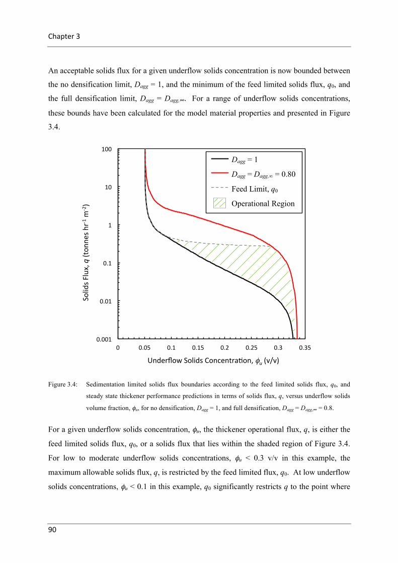
Chapter3

90

An acceptable solids flux for a given underflow solids concentration is now bounded between

the no densification limit, Dagg = 1, and the minimum of the feed limited solids flux, q0, and

the full densification limit, Dagg = Dagg,∞. For a range of underflow solids concentrations,

these bounds have been calculated for the model material properties and presented in Figure

3.4.

Figure 3.4: Sedimentation limited solids flux boundaries according to the feed limited solids flux, q0, and

steady state thickener performance predictions in terms of solids flux, q, versus underflow solids

volume fraction, φu, for no densification, Dagg = 1, and full densification, Dagg = Dagg,∞ = 0.8.

For a given underflow solids concentration, φu, the thickener operational flux, q, is either the

feed limited solids flux, q0, or a solids flux that lies within the shaded region of Figure 3.4.

For low to moderate underflow solids concentrations, φu < 0.3 v/v in this example, the

maximum allowable solids flux, q, is restricted by the feed limited flux, q0. At low underflow

solids concentrations, φu < 0.1 in this example, q0 significantly restricts q to the point where

0.001

0.01

0.1

1

10

100

0 0.05 0.1 0.15 0.2 0.25 0.3 0.35

SolidsF

lux,q(ton

nesh

r-1m

-2)


Dagg = 1


Feed Limit, q0

Operational Region

ThickenerModelling

91

aggregate densification no longer provides a solids flux performance enhancement, q =

q(Dagg = 1) = q0.


Knowledge of the solids residence time is unknown prior to determining the sedimentation

limited settling flux. As tres is sensitive to the densification rate parameter, A, it is expected

that tres will be close to an un-densified value when A is small, say tres = tres,0, and will

approach the fully densified case as A increases, tres = tres,∞.

Usher et al. (2009) assumed the aggregates enter the thickener in a fully densified state thus

implying the material properties, in particular the hindered settling function, are no longer a

function of time, R = R(φ) only. Therefore qs could easily be determined without prior

knowledge of tres. tres can then subsequently be determined using equation 2.117. This

method is acceptable if, for the given rate of aggregate densification, the overall solids

residence time, tres, is sufficient for full densification, Dagg(z = 0) = Dagg,∞ (subject to the

limitations identified in section 3.4.3.

For a given underflow solids concentration, φu, full densification may not be possible as the

maximum tres is restricted by the feed limited solids flux. Hence, tres needs to be quantified

when calculating qs. In order to solve equation 3.1, an iterative approach is performed in

which the solids residence time is adjusted until φ(z) produces the feed and bed heights, hf

and hb, specified in the model inputs. Under certain scenarios, the specified bed height is

unobtainable due to the restriction of the feed limiting solids flux and maximum solids

residence time. For these scenarios, the model predicts the steady state solution for the

maximum bed height obtainable. The algorithm used to solve for tres is outlined in section

3.7.

3.4.5 Overall sedimentation flux

Based on the knowledge that the solids flux at a given solids concentration increases with

aggregate densification, if the minimum value of q over the domain from φ0 to φu is greater

than q0, then q0 limits the solids flux. Alternatively if the minimum value of q over the same

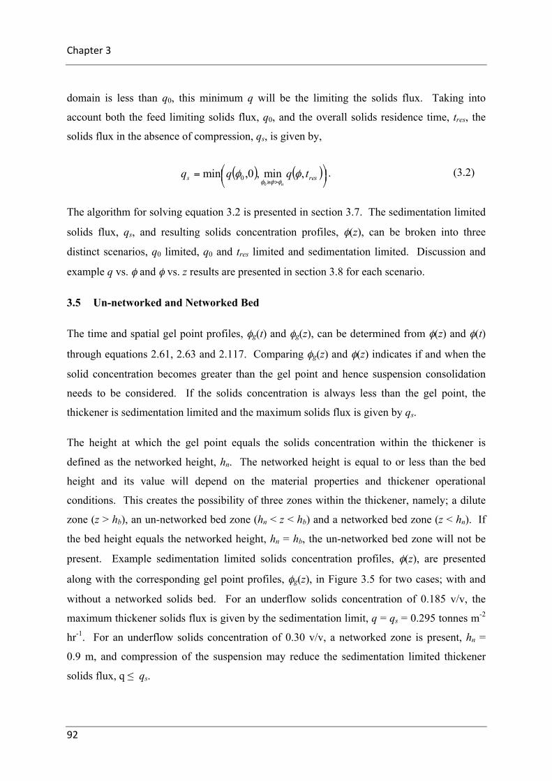
Chapter3

92

domain is less than q0, this minimum q will be the limiting the solids flux. Taking into

account both the feed limiting solids flux, q0, and the overall solids residence time, tres, the

solids flux in the absence of compression, qs, is given by,

. (3.2)

The algorithm for solving equation 3.2 is presented in section 3.7. The sedimentation limited

solids flux, qs, and resulting solids concentration profiles, φ(z), can be broken into three

distinct scenarios, q0 limited, q0 and tres limited and sedimentation limited. Discussion and

example q vs. φ and φ vs. z results are presented in section 3.8 for each scenario.

3.5 Un-networked and Networked Bed

The time and spatial gel point profiles, φg(t) and φg(z), can be determined from φ(z) and φ(t)

through equations 2.61, 2.63 and 2.117. Comparing φg(z) and φ(z) indicates if and when the

solid concentration becomes greater than the gel point and hence suspension consolidation

needs to be considered. If the solids concentration is always less than the gel point, the

thickener is sedimentation limited and the maximum solids flux is given by qs.

The height at which the gel point equals the solids concentration within the thickener is

defined as the networked height, hn. The networked height is equal to or less than the bed

height and its value will depend on the material properties and thickener operational

conditions. This creates the possibility of three zones within the thickener, namely; a dilute

zone (z > hb), an un-networked bed zone (hn < z < hb) and a networked bed zone (z < hn). If

the bed height equals the networked height, hn = hb, the un-networked bed zone will not be

present. Example sedimentation limited solids concentration profiles, φ(z), are presented

along with the corresponding gel point profiles, φg(z), in Figure 3.5 for two cases; with and

without a networked solids bed. For an underflow solids concentration of 0.185 v/v, the

maximum thickener solids flux is given by the sedimentation limit, q = qs = 0.295 tonnes m-2

hr-1. For an underflow solids concentration of 0.30 v/v, a networked zone is present, hn =

0.9 m, and compression of the suspension may reduce the sedimentation limited thickener

solids flux, q ≤�qs.

( ) ( )⎟⎠⎞⎜

⎝⎛=

>≥ress tqqq

u

,min,0,min0

0 φφφφφ

ThickenerModelling

93

Figure 3.5: Profile of solids concentration φ and solids gel point φg vs. height z for the case of sedimentation

limited settling where (left) q = 0.29 tonnes m-2 hr-1, φu = 0.18 v/v, A(z > hb) = 0, A(z � hb) =

10-4 s-1 and Dagg∞ = 0.8 (right) q = 0.29 tonnes m-2 hr-1, φu = 0.30 v/v, A(z > hb) = 0, A(z � hb) = 10-4

s-1 and Dagg∞ = 0.8. The horizontal dashed lines indicate the (uniform) bed and networked

heights, hb (2 m) and hn (0 and 0.89 m).

3.6 Compression Theory

The solids flux calculated by sedimentation alone is often not achieved due to the

compressibility of the suspension, which limits the maximum possible underflow solids

concentration. As discussed above, compression calculations are required if a networked

zone is present within the thickener. The technique used to account for compression involves

integration of the differential equations determined from fundamental dewatering theory.

The differential equations used to account for compression in the presence of dynamic

aggregate densification are (Zhang et al. 2013);

,

(3.3)

and

0

1

2

3

4

5

0 0.05 0.1 0.15 0.2

Height,z(m

)


phi

phig

0

1

2

3

4

5

0 0.1 0.2 0.3

Height,z(m

)


phi

Series4

( )( )

( )

( )φ

φ

φ

φφφφ

φρφ

∂

∂∂

∂−⎟⎟⎠

⎞⎜⎜⎝

⎛−

−−Δ

=resy

res

resy

u

res

res tPttP

qtRg

dtd

,

,111, 2

2

hb

φu

φ0 φ(z)

φg(z)

hb

φu

φ0

hn

φ(z)

φg(z)

Chapter3

94

.

(3.4)

These differential equations describe the change in solids concentration with time and height

within the suspension bed of a thickener for a given solids flux, q, and underflow solids

concentration, φu. The determination of the solids flux, q, required to produce a steady state

suspension bed height, hb, at an underflow solids concentration, φu, is performed in two parts.

The first part deals with sedimentation above the networked bed height while the second part

considers compression in the networked suspension bed.

Sedimentation theory is used to determine the networked bed height, hn, the solids residence

time at the top of the networked bed, tn, and the concentration profiles for the dilute and un-

networked bed zone (z > hn). Within these zones, aggregates are un-networked and settling is

sedimentation limited. If there is a networked bed, the differential equations, 3.3 and 3.4, are

integrated simultaneously from z = hn to z = 0 subject to the boundary condition, φ(hn,tn) =

φg(tn). This integration determines the solids concentration profile within the networked

zone, φ(z) for z < hn.

An alternative description of equation 3.3 can improve computational speed. The inverted

differential equation, shown below,

, (3.5)

relates the change in time with solids concentration in the thickener, dtres/dφ, for a given

steady state solids flux, q, and underflow solids concentrations, φu. The differential equation

is integrated from the top of the networked bed, φ = φg to φu.

( )( )

( ) ( )φ

φ

φ

φφφ

φφ

φρφ

ddt

ttPtP

qtRg

dzd

res

res

resyresy

u

res

∂

∂+

∂

∂

⎟⎟⎠

⎞⎜⎜⎝

⎛−

−−Δ

= ,,

11,

2

( )

( )( )

( )res

resy

u

res

resy

res

ttP

qtRg

tP

ddt

∂

∂−⎟⎟⎠

⎞⎜⎜⎝

⎛−

−−Δ

∂

∂

=,11

1,

,

22

φ

φφφ

φφρ

φ

φ

φ

ThickenerModelling

95

Calculations are performed with an initial guess for q and iteratively adjusted until the solids

concentration at the base of the thickener equals the underflow solids concentration,

φ(z = 0) = φu. The value of q is bounded between the no densification solution, q(Dagg = 1),

and the minimum of the sedimentation limited settling flux, qs, and fully densified solid flux,

q(Dagg,∞), for the given φu.

At solids concentrations equal to or just above the gel point, it is possible for the suspension

to be sedimentation limited although networked. In order to determine the limiting

mechanism, a simplified version of the entropy condition outlined by Burger has been

implemented in which ensures the solids concentration profile is smooth and continuous

throughout the suspension bed. The limiting mechanism of dewatering is determined by

comparison of the change in height with respect to solids concentration, dz/dφ, when applying

both sedimentation and compression theory. The thickener is sedimentation limited until

|dz/dφ|sedimentation < |dz/dφ|compression, after which compression is the limiting mechanism of

dewatering. The height and solids concentration at which the transition from sedimentation

to compression limited operation occurs is defined as hlimit and φlimit. Equation 3.4 and 3.5 are

integrated from z = hlimit and φ = φ limit to z = 0 and φ = φu. The algorithm used is presented in

section 3.7. Example predicted solids concentration profiles for

φu = 0.30 and 0.32 v/v are shown in Figure 3.6. At φu = 0.30 v/v, the suspension bed is both

permeability and compression limited, with the transition occurring at z = hn = 1.85 m and

φ = φg = 0.15 v/v. For φu = 0.32 v/v, the entire suspension bed is compression limited, hb = hn

and φ(hb) = φg(hb).

Chapter3

96

Figure 3.6: Profile of solids concentration φ and solids gel point φg vs. height z for the case of compression

limited settling where (left) q = 0.17 tonnes m-2 hr-1, φu = 0.30 v/v, A(z > hb) = 0, A(z � hb) = 10-3s-1

and Dagg∞ = 0.8 (right) q = 0.07 tonnes m-2hr-1, φu = 0.32 v/v, A(z > hb) = 0, A(z � hb) = 10-3s-1 and

Dagg∞ = 0.8. The horizontal dashed lines indicate the (un-networked) bed and networked bed

heights, hb (2 m) and hn (0 and 1.85 m).

3.7 Model Algorithm

The computational algorithm that can be applied to predict steady state thickening

performance with dynamic aggregate densification is now described. The algorithm is split

into the core and subsections; standard steady state thickener, dilute zone, un-networked bed

zone and networked bed zone. A block flow diagram representing the main steps within the

core algorithm is depicted in Figure 3.7. An alternative algorithm for determining the solids

flux for a thickener operated under compressional limits is also presented. This alternative is

computationally less demanding however, is less accurate due to the inherent approximations

and assumptions.

3.7.1 Core algorithm

1. Define the model inputs:

Thickener geometry including feed height, hf. (in this case, straight walled thickener)

Material properties, R(φ), Py(φ), A, Dagg,∞, ρsol, ρliq

Operational parameters including hb and φ0.

0

1

2

3

4

5

0 0.1 0.2 0.3

Height,z(m

)


phi

phig

φ(z)

φg(z)

hb

hn

φ0

φu0

1

2

3

4

5

0 0.1 0.2 0.3

Height,z(m

)


phi

phig

φ(z)

φg(z)

φu

φ0

hb

ThickenerModelling

97

2. Create a φu list:

Create a list of underflow solids volume fractions, φu, with values bounded between

the initial solids volume fraction, φ0, and a high value that exceeds the maximum

achievable underflow solids concentration (e.g. φcp).

3. Determine Solids Flux Boundaries:

For each underflow solids concentration, φu, determine the solids flux boundaries

using the Standard steady state thickener algorithm.

a. Determine the minimum solids fluxes;

qs,min = qs(Dagg = 1) and qmin = q(Dagg =1)

b. Determine the maximum solids fluxes;

qs,max = qs(Dagg = Dagg,∞) and qmax = q(Dagg = Dagg,∞)

4. Determine the Sedimentation Limited Settling Flux:

For each underflow solids concentration, φu, determine the sedimentation limited

settling flux, qs, using the Sedimentation limited flux algorithm

5. Determine the Gel Point Profile:

For each underflow solids concentration,

a. Determine z(t) from φ(z) and φ(t)

b. Determine φg(z) from z(t) via eq. 2.61 and 2.63

6. Determine the Solids Flux:

For each underflow solids concentration; If φu ≥ φg(z = 0), then q = qs. Else, if φu <

φg(z = 0) then;

a. Determine the relevant bed height bounds zmin and zfree,

i. The minimum bed height required to achieve φu, defined as zmin = z(φg),

is determined by the Compressibility algorithm with q = qmin.

ii. The bed height beyond which thickener operation is sedimentation

limited is defined as zfree = z(φg), is determined by the Compressibility

algorithm with q = min[0.99qs, qmax]

b. Create a list of q values corresponding to the list of φu values such that;

i. If hb < zmin, φu is unattainable and there was no corresponding q value

ii. If zequil ≤ hb ≤ zmin, q is determined via Compressibility algorithm

Chapter3

98

iii. If hb ≥ zmin, then q = qs

An alternative method that utilises the standard steady state thickener algorithm can be

applied to estimate an upper bound for thickener performance with significantly less

computational overhead, but subject to a loss of accuracy. When applying the Alternative

networked bed method algorithm, step 6 becomes;

6. Determine the Solids Flux:

For each underflow solids concentration; If φ(z = 0) ≤ φg(z = 0), then q = qs. Else, if

φ(z = 0) > φg(z = 0) then, q is determined via Alternative networked bed algorithm.

ThickenerModelling

99

Figure 3.7: Block flow diagram of core algorithm used to predict steady state thickener performance in terms

of solids flux vs. underflow solids concentration as well as solids concentration profiles.

1.Definethemodelinputs• Py(φ),R(φ),Δρ,A,Dagg,∞,hb,

hf,φ0

2.Createaφulist

3.Determinesolidsfluxboundaries

• qs,min,qs,max,qmin,qmax

4.Determinesedimentanonlimitedsolidsflux

• qs,φ(z),t(z)

5.Determineφg(z)

6.DeterimineSolidsflux

Chapter3

100

3.7.2 Standard steady state thickener algorithm

This is a reproduction of the algorithm for steady state thickener performance prediction with

time independent material properties as presented in Usher and Scales (2005). Note, that for

a cylindrical thickener with constant cross sectional area, α(z) = 1 in equation 2.113.

1. For each underflow solids concentration, φu, the minimum sedimentation limited flux,

qs, is determined by application of eq. 3.1 for all solids concentrations, φ, ranging

from φ0 to φu as described in the Sedimentation Theory.

2. The relevant bed height bounds zequil and zmin are calculated for each specified

underflow solids concentration, φu, where φu > φg. The minimum bed height required

to achieve φu, defined as zequil = z(φg), is determined by integration of eq. 2.113 with q

= 0. The bed height beyond which thickener operation is permeability limited is

defined as zmin = z(φg). For a cylindrical vessel (α(z) = 1), zmin is determined by

integration of eq. 2.113 with q = 0.99qs (Note that if q ≥ qs, then eq. 2.113 cannot be

solved to uniquely satisfy the boundary conditions). When the thickener has a

converging base (α(z) < 1), it is more difficult to avoid unstable integrations. In this

case, the value of zmin is initially guessed as 0, and then iteratively determined as zmin

= z(φg), by integration of eq. 2.113 with q = α(zmin)qs. eq. 2.113 is iteratively solved

until the variation of zmin between iterations is insignificant (e.g. <10−8).

3. A list of q values is created corresponding to the list of φu values such that; if φu < φg

then q = min[qs,q(φ0,t=0)]. Else, if φu ≥ φg then;

a. if hb < zequil, φu is unattainable and there is no corresponding q value,

b. if zequil ≤hb < zmin, q is determined via a shooting method described below and

c. if hb ≥zmin, then q = qs.

The shooting method for determining q, given φu and hb, involved initially setting the left and

right bounds of q such that ql = 0 and qr = α(zfree)qs. Using the midpoint between ql and qr as a

guess for q, qguess = (ql + qr)/2, eq. 2.113 is solved to determine z(φg). If z(φg) > hb, then qr =

ThickenerModelling

101

qguess, else ql = qguess. The process is iteratively repeated until the required accuracy was

achieved (e.g. |qr −ql|<10−8).

3.7.3 Sedimentation limited solids flux algorithm

The algorithm for determining the sedimentation limited solids flux, qs, for a given underflow

solids concentration, φu, is described below:

1. Determine feed limited solids flux:

Determine q0 = q(φ0,t = 0) via eq. 3.1.

2. Determine maximum overall solids residence time:

If qs,max ≤ q0, then

a. Dagg,max = Dagg,∞ and tmax = (φu/qs,min).hf

b. Else tmax is given when q0 = min[(q(φ, t))] according to eq. 3.1 evaluated over

the solids concentration range from φ0 to φu.

Determine Dagg,max from tmax using eq. 2.61

3. Determine mode:

Solve Dilute zone algorithm evaluated at q = q0;

a. If [q(φ, t)] = q0 or tb ≥ tmax, Mode 1: q0 limited.

b. Else with qs = q0, solve eq. 3.1 and 2.117 for φ(t) and φ(z) for all solids

concentrations, φ, and time, t, ranging from φ0 to φu and tb to tmax. If z(tres) ≥ 0,

Mode 2: q0 and tres limited, else Mode 3: Sedimentation limited.

4. Determine qs:

Determine φ(t), z(t) and hence φ(z) (parametrically in terms of t)

a. If Mode 1: qs =q0. Solve Dilute zone algorithm with hb = 0 and

b. Mode 2: Solve Eqs. 3.1 and 2.117 for φ(t) and φ(z) for all solids

concentrations, φ, and time, t, ranging from φ0 to φu and tb to tmax with qs = q0.

Iterate on hb via midpoint shooting method until z(tmax) = 0 or within

reasonable accuracy, i.e. | z(tmax) | < 10-5

c. Mode 3: Solve Dilute zone and Permeability Zone algorithms

uφφφ ≤≤0min

Chapter3

102

3.7.4 Dilute zone algorithm

The algorithm for determining both φ(t) and φ(z) within the dilute zone, z ≥ hb, for a given q

and φu is described below:

1. Initially set the left and right bounds of tres such that tres,l = 0 and tres,r = (φ0/qmin)(hf-hb)

2. Using the midpoint between tres,l and tres,r as a guess for tres, tres,guess = (tres,l+tres,r)/2,

φ(t) and φ(z) is determined by application of eq. 3.1 and 2.117 for all solids

concentrations, φ, and time, t, ranging from 0 to φ0 and 0 to tres,guess.

3. If z(tres) > hb, then tres,l = tres,guess, else tres,r = tres,guess.

4. The process is iteratively repeated until the required accuracy was achieved (e.g.

|z(tres) – hb| < 10-5).

5. The time an aggregate spends within the dilute zone of the thickener, is noted as tb.

3.7.5 Permeability zone algorithm

The algorithm for determining both φ(t) and φ(z), for a given φu and hb in the absence of

compression is described below:

1. Initially set the left and right bounds of qs such that qs,l = qs,min and qs,r = qs,max

2. Using the midpoint between qs,l and qs,r as a guess for qs, qs,guess = (qs,l+qs,r)/2,

a. Solve for φ(t) and φ(z) for z > hb via Dilute Zone algorithm.

b. Solve for φ(t) and φ(z) for z < hb by,

i. Initially set the left and right bounds of tres such that tres,l = tb and tres,r =

tmax

ii. Using the midpoint between tres,l and tres,r as a guess for tres, tres,guess =

(tres,l+tres,r)/2, φ(t) and φ(z) is determined by application of eq. 3.1 and

2.117 for all solids concentrations, φ, and time, t, ranging from φ0 to φu

and tb to tres,guess.

iii. If z(tres) > hb, then tres,l = tres,guess, else tres,r = tres,guess.

iv. The process is iteratively repeated until the required accuracy is

achieved (e.g. |z(tres)| < 10-5).

ThickenerModelling

103

c. If qs,guess < [q(φ, tres)] then qs,r = qs,guess, else qs,l = qs,guess.

d. The process is iteratively repeated until the required accuracy is achieved (e.g.

| qs,guess – [q(φ, tres)] | < 10-5).

3.7.6 Compressibility algorithm

The algorithm for determining both φ(t) and φ(z), for a given φu and hb including the effect of

compression is described below:

1. Initially set the left and right bounds of q such that ql = qmax and qr = min[0.99qs, qmax]

2. Using the midpoint between ql and qr as a guess for q, qguess = (qr+ql)/2,

a. Solve φ(t) and φ(z) for z ≥ hb using the Dilute Zone algorithm.

b. Calculate both q(φ, t = ∞) and q(φ, tb) for all solids concentrations, φ, ranging

from φ0 to φu using eq. 3.1.

i. If (q(φ, tb)) ≥ qguess, then there is no un-networked zone.

ii. Else if (q(φ, t = ∞)) ≤ qguess, solve φs(t) and φ s(z) for z ≤ hb using

the Permeability Zone algorithm.

iii. Else tmax is given by (q(φ, t)) = qguess. Solve φ s(t) and φ s(z) for z

≤ hb using the Permeability Zone algorithm at tres = tmax, noting a full

bed may not be obtained.

c. Solve φg(z) (parametrically in terms of t) via eq. 2.61 and 2.63. Subsequently

solve φ(t) and φ(z). In turn determine hn, tres(hn) and φ(hn).

d. From φ s(t), determine (dt/dφ)s via finite difference.

e. Create a list of φ values from φs(hn, tb) to φu with spacing Δφ

f. Numerically solve for t via: tn+1 = tn + Δφ.max[(dt/dφ)s, dt/dφ] where dt/dφ is

given by eq. 3.5.

g. Using eq. 2.117 convert φ(t) to φ(z) via trapezoidal method

3. If z(tres) > 0, then ql = qguess, else qr = qguess.

uφφφ ≤≤0min

uφφφ ≤≤0min

uφφφ ≤≤0min

uφφφ ≤≤0min

uφφφ ≤≤0min

Chapter3

104

4. The process is iteratively repeated until the required accuracy was achieved

(e.g. | z(tres)| < 10-5).

3.7.7 Alternative networked bed method

The algorithm for solving the solids concentration distribution in the suspension bed is

complex and computationally demanding. However, a close approximation can be more

easily determined by equating solids residence times.

For a given rate of aggregate densification, there is a solids residence time required to achieve

a given extent of aggregate densification. Similarly using time independent material

properties, a solids residence time can be calculated for a range of underflow solids

concentrations for a given Dagg. Equating the two solids residence times provides an

approximation of the solids flux achievable for a given underflow solids concentration.

The algorithm for this approximation method used to determine q vs. φu for a given hb and A

is presented below:

1. A list of scald aggregate diameters, Dagg, is created with values bounded between the

un-densified value, Dagg = 1, and the fully densified value, Dagg = Dagg,∞.

2. For each Dagg value;

a. Determine the solids residence time required to reach Dagg via eq. 2.61

b. Apply the Solids flux boundaries algorithm for the Dagg value over the range

of φu values to find q(Dagg) vs. φu

c. Calculate the solids residence time for each q vs. φu point via eq. 2.117,

tres(φu,Dagg)

d. Match tres in (a.) with a tres in (c.) to determine the correct Dagg and q for the

given φu.

3.8 Outputs: Model Thickener Performance Prediction

An algorithm has been developed in Matlab code to take the above mentioned model inputs

and predict steady state solids flux for a range of underflow solids concentrations. Using this

ThickenerModelling

105

algorithm, a model case study has been performed to demonstrate the impact of time

dependent aggregate densification on steady state thickener performance.

For this case study, Py(φ) and R(φ) curve fits (Figure 3.1) have been used along with feed and

bed heights of 5 and 2 m, and a feed solids concentration of 0.05 v/v (Usher and Scales 2005,

Usher et al. 2009, Zhang et al. 2013, Grassia et al. 2014). Aggregate densification parameters

representing a moderate shear rate have been used, As = A(z > hb) = 0, Abed =

A(z ≤ hb) = 10-4 s-1 and Dagg∞ = 0.8. These values are in agreement with both experimental

observations and measurements in Chapter 4 and previous authors (Usher et al. 2009, van

Deventer et al. 2011). For this case study, only raking within the solids bed is considered

(z ≤ hb). The effects and benefits of shear processes above the bed (As > 0) are considered

and discussed in section 3.9.4 and Chapter 5.

The steady state thickener performance predictions, in terms of solids flux versus underflow

solids volume fraction is shown in Figure 3.8 for operation of a straight walled thickener (no

cross sectional area variation). The effect of process variables such as bed height, feed

concentration, and rate of aggregate densification are investigated and discussed in section

3.8.7. It should be noted, that at high solids fluxes where operation is limited by the feed

solids flux, the specified bed height could not be obtained, and instead the solution represents

a solids flux when operated at the maximum possible bed height.

Chapter3

106

Figure 3.8: Steady state (straight walled) thickener model prediction of the solids flux as a function of

underflow solids volume fraction for A(z > hb) = 0, A(z ≤ hb) = 10-4 s-1, Dagg,∞ = 0.8, φ0 = 0.05 v/v,

hf = 5 m and hb = 2 m. Upper and lower solids flux predictions (Dagg = 1 and Dagg = Dagg,∞) are

also shown.

Both sedimentation and compression theory are combined to predict the limiting steady state

solids flux, q, for a range of underflow solids concentrations, φu. Steady state thickener

operation can be split into five distinct modes of operation, each of which will be discussed in

turn.

As underflow solids concentration increases, the predicted steady state thickener solids flux

with dynamic densification transitions from mode 1 through to mode 5. Note that the

underflow solids concentration in which the transition between modes occurs is dependent on

the material properties and operational parameters. In the following discussions, the stated

0.001

0.01

0.1

1

10

100

0 0.05 0.1 0.15 0.2 0.25 0.3 0.35

SolidsF

lux,q(ton

nesh

r-1m

-2)


q_Dagg0

q_Dagginf

q

qk

qk_feed

Dagg = 1


q

qs

q0 limit

ThickenerModelling

107

underflow solids concentrations for transition between modes is unique to the model inputs as

described in section 3.3.

3.8.1 Alternative algorithm for networked bed

The algorithm for solving the solids concentration distribution in the suspension bed is

complex and computationally demanding. However, using time in-dependent material

properties and equating solids residence times can easily determine a close approximation.

The algorithm for calculating the solids flux via this alternative method is presented in

section 3.7.7. The predicted steady state thickener performance using this less

computationally demanding algorithm is presented in Figure 3.9.

Chapter3

108


underflow solids volume fraction for A(z > hb) = 0, A(z ≤ hb) = 10-4 s-1, Dagg,∞ = 0.8, φ0 = 0.05 v/v,

hf = 5 m and hb = 2 m. Thickener predictions have been performed using two algorithms, one

more computationally demanding than the other. Upper and lower solids flux predictions

(Dagg = 1 and Dagg = Dagg,∞) are also shown.

This alternative networked bed method assumes; no un-networked bed zone (hn = hb), zero

solids residence time within the dilute zone, tb = tn = 0, and assumes the aggregates are at the

final densification state across the entire suspension bed. Due to these assumptions, this

alternative method will be less computationally demanding, but provides an overestimate of

the solids flux, q, for a given underflow solids concentration, φu, as shown in Figure 3.9.

3.8.2 Mode 1: Permeability and q0 limited

At low underflow solids concentrations, φu < 0.08 v/v for this model material, aggregate

densification does not provide any performance enhancement in terms of solids flux. Here, qs

0.001

0.01

0.1

1

10

100

0 0.05 0.1 0.15 0.2 0.25 0.3 0.35

SolidsF

lux,q(ton

nesh

r-1m

-2)


Series9

Dagg = 1


Feed Limit

A = 10-4 s-1, q = qs

A = 10-4 s-1

Approximation

ThickenerModelling

109

will always be equal to the feed flux, q0, and the un-densified (Dagg = 1) solids flux. This is

inherently due to the nature of the solid flux curves, q vs. φ, in which there is an absence of a

local minima and maxima causing equation 3.1 to be a minimum at φ = φ0 over the solids

concentration range φ0 to φu for all t. To illustrate this, an example q vs. φ and φ(z) is shown

in Figure 3.10 for an underflow solids concentration, φu, of 0.06 v/v.

Figure 3.10: Solids flux, q (tonnes hour-1 m-2), vs. solids concentration, φ (v/v), and corresponding solid

concentration profile, φ(z) for an underflow solids concentration of 0.06 v/v, operating under feed

flux limitations. Aggregate densification parameters of Dagg,∞ = 0.8, A(z > hb) = 0 and

A(z ≤ hb) = 10-4 s-1.

Due to the lack of a local minima and maxima in the solid flux curves, q vs. φ, only one

solids concentration, φ, over the entire range from 0 to φu, satisfies equation 3.1 for a given

underflow solids concentration, solids residence time and solids flux. Hence thickeners

operated within this region will not have a bed present (either un-networked or networked);

instead the suspension will dilute due to aggregate densification from the feed down to the

base of the thickener. The solids concentration profiles for underflow solids concentrations

of 0.06, 0.07, and 0.08 v/v are presented in Figure 3.11.

0.1

1

10

100

0 0.02 0.04 0.06

SolidsF

lux,q(ton

nesh

r-1m

-2)


q(Dagg0)q(Dagginf)Phi

φ0 φu

q(Dagg=1)

q(Dagg=Dagg,∞)

φrange

0

1

2

3

4

5

0 0.02 0.04 0.06

Height,z(m

)


phi0

phiuφ0

φu

Chapter3

110

Figure 3.11: The profile of the height in the thickener vs. the solids volume fraction – for comparatively

‘small’ underflow solids concentrations, φu = 0.06, 0.07 and 0.08 v/v, in which the thickener is

operated under feed flux limitations and no bed is achievable. Aggregate densification parameters

of Dagg,∞ = 0.8, A(z > hb) = 0 and A(z ≤ hb) = 10-4 s-1.

3.8.3 Mode 2: Permeability, q0 and tres limited

The solids concentration increases with time within the suspension bed due to the dynamic

behaviour of aggregate densification. This increase in solids concentration may cause the

specified thickener operational bed height to be unattainable. This occurs at low to moderate

solids fluxes, 0.08 < φu < 0.16 v/v, where for large t, no solids concentrations within the range

φ0 to φu satisfies equation 3.1 for the given q and φu. This is due to the nature of the solids

flux curves, q vs. φ, whereby a local minimum is initially present but then disappears as the

calculated q exceeds q0 with densification.

0

1

2

3

4

5

0 0.02 0.04 0.06 0.08

Height,z(m

)


0.06

0.07

0.08

phi0

phiu

φu

φ0φu

ThickenerModelling

111

For this scenario, qs is given by the feed limited solids flux, qs = q0, and the solids residence

time is given by equation 3.1 evaluated such that q0 = min[q(φ,tmax)] over the solids

concentration, φ, range from φ0 to φu. The bed height is than iterated between 0 and the

specified operational bed height, hb, until tres = tmax. Note, for this operational mode, no

solids flux for the given underflow solids concentration will achieve the specified bed height,

albeit a smaller bed can be achieved. An example solid flux curve, q vs. φ, and

corresponding solids concentration profile, φ(z), for q0 and tres limited operation is illustrated

in Figure 3.12. This illustrated example is for an underflow solids concentration of 0.1 v/v

and solids flux of q = q0 = 0.45 tonnes m-2 hr-1. For this example, tres = tmax = 0.3 hr

restricting the maximum bed height to 0.42 m. Solids concentration profiles for underflow

solids concentrations of 0.10, 0.12, 0.14, and 0.16 v/v are presented in Figure 3.13 illustrating

an increase in obtainable bed height with increasing underflow solids concentration.


concentration profiles, φ(z) for an underflow solids concentration of 0.10 v/v, operating under feed

flux, q0, and solid residence time, tres, limitations. Aggregate densification parameters of Dagg,∞ =

0.8, A(z > hb) = 0 and A(z ≤ hb) = 10-4 s-1.

0.1

1

10

100

0 0.05 0.1

SolidsF

lux,q(ton

nesh

r-1m

-2)



φ0 φu

q(Dagg=1)

q(Dagg=Dagg,∞)

φrange

0

1

2

3

4

5

0 0.05 0.1

Height,z(m

)


phi0

phiu

φ0

φu

Chapter3

112


‘small’ underflow solids concentrations, φu = 0.10, 0.12, 0.14 and 0.16 v/v, in which the thickener

is operated under feed flux and solid residence time limitations. The specified bed height is

unobtainable and smaller beds are achieved. Aggregate densification parameters of Dagg,∞ = 0.8,

A(z > hb) = 0 and A(z ≤ hb) = 10-4 s-1.

q0 and tres limited scenarios only occur when the local minima in q vs. φ exceeds q0 at a

critical solids residence time, tmax, and are thus highly dependent on the rate of aggregate

densification (along with φu and R(φ,t)). For a given underflow solids concentration, a

critical rate of densification parameter, Acrit, exists in which the specified bed height, hb, can

be achieved. At A ≥ Acrit, the solids flux is limited by both q0 and tres, however at smaller

rates, A < Acrit, the solids flux is only limited by the permeability of the suspension as

discussed below.

0

1

2

3

4

5

0 0.05 0.1 0.15

Height,z(m

)


0.1

0.12

0.14

0.16

φu

ThickenerModelling

113

3.8.4 Mode 3: Permeability limited

At moderate underflow solids concentrations (0.17 > φu > 0.20 v/v) thickener performance is

limited only by the permeability of the suspension. This implies that the rate at which the

solids are passed through the thickener is high enough for there to be no transmission of

compressive forces within the suspension bed. The limiting factor is the rate at which the

liquid can escape from the solids network, dictated by the permeability of the suspension.

Unlike Mode 2, permeability limited operation is not limited by q0 or tres. This is due to

either; a small rate of aggregate densification such that q(φ, tres) < q0 meaning a specified bed

height can be obtained, or if min[q(φ, t = ∞)] < q0 as commonly seen at larger underflow

solids concentrations. Figure 3.14 illustrates an example solid flux curve, q vs. φ, and solids

concentration profile, φ(z). The solids concentration profiles, φ(z) for underflow solids

concentrations within the permeability range are displayed in Figure 3.15 .


concentration profile, φ(z) for an underflow solids concentration of 0.18 v/v, operating under

permeability limitations. Aggregate densification parameters of Dagg,∞ = 0.8, A(z > hb) = 0 and

A(z ≤ hb) = 10-4 s-1.

0.01

0.1

1

10

100

0 0.05 0.1 0.15 0.2

SolidsF

lux,q(ton

nesh

r-1m

-2)



φ0 φu0

1

2

3

4

5

0 0.05 0.1 0.15 0.2

Height,z(m

)

SolidsConcentanon,φ(v/v)

phi0phiuphig

φ0

φu

φg(z)

Dagg = 1


φ range

Chapter3

114


‘intermediate’ underflow solids concentrations, φu = 0.17, 0.18, 0.19 and 0.20 v/v, in which the

thickener is operated under permeability limitations. Aggregate densification parameters of

Dagg,∞ = 0.8, A(z > hb) = 0 and A(z ≤ hb) = 10-4 s-1.

As discussed in section 3.6, it is possible for the networked suspension bed to be permeability

limited. For this case, the solids flux is given by the sedimentation limiting solids flux,

q = qs.

3.8.5 Mode 4: Networked permeability and compression limited

At moderate to high underflow solids concentrations, φu between 0.2 and 0.3 v/v in this

example, the suspension bed is comprised of both an un-networked and networked zone. The

un-networked zone is sedimentation limited while the networked zone is at solids

concentrations above the gel point and potentially compression limited. Overall the thickener

performance is limited by both the permeability and the compressibility of the suspension.

0

1

2

3

4

5

0 0.05 0.1 0.15 0.2

Height,z(m

)


0.17

0.18

0.19

0.2

φu

ThickenerModelling

115

Figure 3.16 shows the resultant solids concentration profile, φ(z), for underflow solids

concentrations of φu = 0.20, 0.25 and 0.3 v/v. The transition between sedimentation and

compressional limiting effects can be at a solids concentration greater than the gel point,

indicating some of the networked bed is sedimentation limited. This is the case for underflow

solids concentrations of 0.25 and 0.3 v/v as indicated by the difference in the solids gel point

and sedimentation/compression limit transition line, as shown in Figure 3.16.


‘intermediate to high’ underflow solids concentrations, φu = 0.20, 0.25 and 0.30 v/v, in which the

suspension bed is operated under both permeability and compressibility limitations. Aggregate

densification parameters of Dagg,∞ = 0.8, A(z > hb) = 0 and A(z ≤ hb) = 10-4 s-1.

3.8.6 Mode 5: Compression limited

At high underflow solids concentrations, φu > 0.3 in this example, thickener operation is

compressibility limited. This implies that the solids residence time is sufficient such that

0

1

2

3

4

5

0 0.05 0.1 0.15 0.2 0.25 0.3

Height,z(m

)


0.30.250.2phigphi0

Sedimentanon/Compressionlimittransinon

φg

φ0

φu

φg

Chapter3

116

compressive dewatering can occur over the entire suspension bed. As such, the amount of

compressive force transmitted by the network structure of the suspension bed is the dominant

effect that governs the underflow solids concentration.

Figure 3.17 shows the resultant solids concentration profile, φ(z), for an underflow solids

concentration, φu = 0.31 v/v in which the thickener performance is limited by the

compressibility of the suspension.

Figure 3.17: The profile of the height in the thickener vs. the solids volume fraction – for comparatively ‘high’

underflow solids concentrations, φu = 0.31 v/v, in which the thickener is operated under

compressibility limitations. Aggregate densification parameters of Dagg,∞ = 0.8, A(z > hb) = 0 and

A(z ≤ hb) = 10-4 s-1.

0

1

2

3

4

5

0 0.05 0.1 0.15 0.2 0.25 0.3

Height,z(m

)


0.31

phi0

phiu

phig

z(φ)

φ0

φu

φg(z)

ThickenerModelling

117


As a result of the steady state thickener model prediction method, the solids residence time

within the thickener, tres, is also determined. Figure 3.18 shows the solids residence time

versus underflow solids concentration based on model predictions. Figure 3.18 also displays

the solids residence time for time in-dependent material properties with Dagg = 1 and

Dagg = Dagg,∞. The solids residence time is influenced by competing terms, the solids flux

and the solids concentration profile as shown in equation 2.117. Therefore the solids

residence time is also dependent on the settling mode due to the resultant solids concentration

profiles.

As expected, the solids residence for steady state thickener operation with dynamic

densification transitions between the two time independent solutions from Dagg = 1 to

Dagg = Dagg,∞. The exception here is at low underflow solids concentrations, between φu =

0.07 and 0.1 v/v, where the solids residence time is less for the dynamic case compared to

when fully densified, further discussed below. Overall an increase in solids residence time is

observed with increasing underflow solids concentration as expected due to the decrease in

solids flux.

Chapter3

118

Figure 3.18: Solids residence time, tres (hr), vs. underflow solids concentration, φu (v/v), for hf = 5 m, hb = 2 m,

A(z > hb) = 0, A(z ≤ hb) = 10-4 s-1, Dagg,∞ = 0.8 and φ0 = 0.05 as well as the predicted solids

residence time for time in-dependent material properties with Dagg = 1 and Dagg = Dagg,∞ = 0.8.

The dashed line represents the dilute zone with bed height < hb, the open squares are

sedimentation limited and closed squares are compression limited solution points.

The solids residence time trends within mode 1, φ < 0.08 v/v, can be split into two section, φ

< 0.065 v/v and 0.065 < φ < 0.08 v/v. For φ < 0.065 v/v the solids residence time with

densification is the same as the un-densified case. This is due to the high solids flux

dominating over the average solids concentration resulting in tres solely given by q. Adding

to this, the high flux result in a low solids residence and hence minimal densification occurs.

For 0.065 < φ < 0.08 v/v, a rapid drop in tres is observed due to the integrated solids

concentration profile becoming of similar order to that of the solids flux and hence decreasing

tres. Due to the need of constant operating flux, aggregate densification causes auto-dilution

0.01

0.1

1

10

100

1000

10000

0 0.1 0.2 0.3 0.4

Solidsresiden

cetime,t r

es(h

r)

Underflowsolidsconcentration,φu(v/v)

total

Dagg=1

Dagg=Dagginf

totalpts

totalpermpts

nobedline

tres(Abed=10-4s-1)

tres(Dagg=1)

tres(Dagg=Dagg,∞=0.8)

CLsolution

PLsolution

hb<2m

φ0

ThickenerModelling

119

resulting in the possibility for the solids residence time with time dependent densification to

be lower than the fully densified case.

During modes 2 to 5, φu > 0.16 v/v, a solids bed is present. Initially at φu = 0.08 v/v, the

solids bed is 0 m and grows to the specified bed height, hb, at φu = 0.016 v/v. Further

increase in φu causes an increase in the average solids concentration within the bed, as

discussed above. This increase in solids bed and solids concentration increases the overall

solids residence time. The discontinuity in the solids residence time at the transition between

mode 3 and 4, φu = 0.20 v/v, is due to discontinuity in the solids flux resulting from the

presence of a networked zone within the suspension bed.

The solids residence time within each zone of the thickener; namely the dilute, un-networked

and networked zones are displayed in Figure 3.19. The relative magnitudes of the solids

residence time in each zone can be observed for a given underflow solids concentration,

providing insight into the rate of aggregate densification required within a zone to achieve a

similar final underflow extent of aggregate densification. For example, for lower underflow

solids concentrations, a significant portion of the solids residence time is in the dilute zone

where shear processes could cause aggregate densification and impact performance, as

discussed in Chapter 5. The range of underflow solids concentrations for each mode of

operation is also indicated in Figure 3.19. Each operation mode corresponds to different

limiting factors and is discussed in detail below.

Chapter3

120

Figure 3.19: Overall solids residence time, tres (hr), vs. underflow solids concentration, φu (v/v), for hf = 5 m,

hb = 2 m, A(z > hb) = 0, A(z ≤ hb) = 10-4 s-1, Dagg,∞ = 0.8 and φ0 = 0.05 as well as the predicted

solids residence time in each zone of the thickener

3.9 Impact of Process Variables

Process optimisation aims to maximise the solids throughput and underflow solids

concentration while maintaining overflow clarity and underflow yield stress. Of the model

inputs, suspension bed height, feed concentration and the rate of aggregate densification can

be manipulated in order to optimise the process. Thickener performance subject to variations

in these operational parameters has been predicted. Trends in the predicted thickener

performance as a function of these operational variables have been observed, providing

further knowledge to aid in optimisation.

0.01

0.1

1

10

100

1000

10000

0 0.1 0.2 0.3 0.4

Solidsresiden

cenme,t r

es(hr)

Underflowsolidsconcentranon,φu(v/v)

total

dilute0

un-net

net

Feed

totalpts

totalpermpts

nobedline

zoneboundaries

φ0

Total

Dilute zone

Un-networked zone

Networked Zone

Feed Concentrations

CL solution

PL solution

Reduced bed height

Mode Boundaries

Mod

e 1

Mod

e 2

Mod

e 3

Mod

e 4

Mod

e 5

ThickenerModelling

121

3.9.1 Suspension bed height

Steady state (straight walled) thickener model prediction of the solids flux as a function of

underflow solids volume fraction has been determined for a range of suspension bed heights,

hb, as shown in Figure 3.20.

As expected and in agreement with previous models (Usher and Scales 2005, Usher et al.

2009) an increase in the suspension bed height results in the potential for increased underflow

solids concentration. Also for a given underflow solids concentration, the increase in

suspension bed height results in an increase in the maximum solids flux, q. Thickener

performance increase due to suspension bed is limited by the feed height (hb cannot exceed

hf) and the feed limiting flux, q0.

The solids residence time, tres, as a function of underflow solids concentration, φu, for bed

heights, hb, of 1, 2, and 4 m is shown in Figure 3.21. As the suspension bed height is

increased, both the average solids concentration and the solids flux increases. This results in

minimal difference between solids residence times for different bed heights at most


Chapter3

122


underflow solids volume fraction for different bed heights, hb = 1, 2 and 4 m. Aggregate

densification and thickener operation parameters of A(z > hb) = 0, A(z ≤ hb) = 10-4 s-1, Dagg,∞ = 0.8

and φ0 = 0.05 v/v were used. Upper and lower solids flux predictions (Dagg = 1 and Dagg = Dagg,∞)

are also shown.

0.001

0.01

0.1

1

10

100

0 0.05 0.1 0.15 0.2 0.25 0.3 0.35 0.4

SolidsF

lux,q(ton

nesh

r-1m

-2)


1 1

2 2

4 4Dagg=0.8

φ0

hb Perm. Comp.

Dagg = 1

ThickenerModelling

123

Figure 3.21: Solids residence time, tres (hr), vs. underflow solids concentration, φu (v/v), for hb = 1, 2 and 4 m,

A(z > hb) = 0, A(z ≤ hb) = 10-4 s-1, Dagg,∞ = 0.8 and φ0 = 0.05 v/v.

3.9.2 Feed concentration


underflow solids volume fraction has been determined for a range of feed solids

concentrations, φ0, as shown in Figure 3.22 (and Figure 3.23 separately). A low φ0 value,

φ0 = 0.005 v/v, has been included in order to demonstrate the impact of a very low feed solids

concentration where φ0 is less than the peak in the solids flux function.

As expected, at high underflow solids concentrations, the thickener is compression limited

and the feed solids concentration has little to no impact on overall thickener performance. At

low to moderate underflow solids concentration, the solids flux is given by the feed limited

solids flux, q0, and hence dependent on φ0. q0 is proportional to the flux function and hence

0.01

0.1

1

10

100

1000

10000

0 0.1 0.2 0.3 0.4

Solidsresiden

cenme,t r

es(hr)


φ0

Reducedbedheight

hb tres Perm. Comp.

1

2

4

Chapter3

124

the optimum feed solids concentration, φ0,opt., corresponds to the peak in the flux function

curve. For the model material, φ0,opt. = 0.012 v/v. Operation at feed solids concentrations

either side of φ0,opt. results in a decreased q0 and hence a decrease in the potential maximum

thickener solids flux, q.

If operating under feed flux limitations, an increase in thickener operational solids flux can be

achieved via altering the feed solids concentration so that φ0 = φ0,opt.. However, due to the

comparatively large gradient in the flux functions at solids concentrations less than this

minimum, ait is recommended to operate at a feed solids concentration slightly above this.

Any slight decreases in the feed solids concentrations due to upstream variances or

disturbances can cause the solids flux to drastically decrease causing un-stable operation.

The solids residence time vs. underflow solids concentration for various feed concentrations

is shown in Figure 3.24.

ThickenerModelling

125


underflow solids volume fraction for different feed concentrations, φ0 = 0.005, 0.02, 0.05 and 0.08

v/v. Aggregate densification and thickener operation parameters of A(z > hb) = 0, A(z ≤ hb) =

10-4 s-1, Dagg,∞ = 0.8, hf = 5 m and hb = 2 m were used. Upper and lower solids flux predictions


0.001

0.01

0.1

1

10

100

0 0.05 0.1 0.15 0.2 0.25 0.3 0.35 0.4

SolidsF

lux,q(ton

nesh

r-1m

-2)

UnderflowSolidsConcentranon,φ(v/v)

φ0 Sed. Comp.

0.005 0.02 0.05 0.08

Bounds q0 limit

Chapter3

126


underflow solids volume fraction for different feed concentrations, φ0 = 0.005, 0.02, 0.05 and 0.08

v/v. Aggregate densification and thickener operation parameters of A(z > hb) = 0, A(z ≤ hb) =

10-4 s-1, Dagg,∞ = 0.8, hf = 5 m and hb = 2 m were used. Upper and lower solids flux predictions


0.001

0.01

0.1

1

10

100

0 0.1 0.2 0.3 0.4

SolidsF

lux,q(ton

nesh

r-1m

-2)


0.001

0.01

0.1

1

10

100

0 0.1 0.2 0.3 0.4

SolidsF

lux,q(ton

nesh

r-1m

-2)


φ0 = 0.02 v/v

0.001

0.01

0.1

1

10

100

0 0.1 0.2 0.3 0.4

SolidsF

lux,q(ton

nesh

r-1m

-2)


φ0 = 0.05 v/v

0.001

0.01

0.1

1

10

100

0 0.1 0.2 0.3 0.4

SolidsF

lux,q(ton

nesh

r-1m

-2)


φ0 = 0.08 v/v

φ0 = 0.005 v/v

ThickenerModelling

127

Figure 3.24: Solids residence time, tres (hr), vs. underflow solids concentration, φu (v/v), for hb = 2 m,

A(z > hb) = 0, A(z ≤ hb) = 10-4 s-1, Dagg,∞ = 0.8 and φ0 = 0.005, 0.02, 0.05 and 0.08 v/v.

3.9.3 Rate of aggregate densification


underflow solids volume fraction has been determined for a range of aggregate densification

rate parameters, A (s-1), as shown in Figure 3.25. The solids residence time vs. underflow

solids concentration for various rates of aggregate densification is shown in Figure 3.26.

As expected, the increase in the rate of aggregate densification results in an increase in the

solids flux for a given underflow solids concentration up to the feed flux limit, q0. At high

rates of aggregate densification, the feed flux limit is dominant for a larger range of


0.01

0.1

1

10

100

1000

10000

0 0.1 0.2 0.3 0.4

Solidsresiden

cenme,t r

es(hr)


φ0 Dilute Sed. Comp.

0.005 0.02 0.05 0.08

φ0φ0φ0φ0

Chapter3

128

According to the model assumption of line settling, all material moves directly away from the

feed height without mixing. However, in real systems there are aggregate density

distributions, flow of particles in all directions and mixing effectively causing densification at

the feed height. Alternatively, densification at the feed height can be caused by shear within

the feedwell, both resulting in an effective initial scaled aggregate diameter, Dagg,0, less than

1. Under these conditions, the feed limiting flux would be increased, allowing for an overall

increase in thickener performance. Prediction of Dagg,0 < 1 is presented in section 3.9.5.


underflow solids volume fraction for rates of aggregate densification, A(z ≤ hb) = 10-5, 10-4, 10-3

s-1. Aggregate densification and thickener operation parameters of Dagg,∞ = 0.8, A(z > hb) = 0, hf =

5 m, hb = 2 m and φ0 = 0.05 v/v were used. Upper and lower solids flux predictions (Dagg = 1 and

Dagg = Dagg,∞) are also shown.

0.001

0.01

0.1

1

10

100

0 0.05 0.1 0.15 0.2 0.25 0.3 0.35

SolidsF

lux,q(ton

nesh

r-1m

-2)


Dagg = 1 Dagg,∞ Feed limit Boundaries

Perm. Limited

Comp. Limited

ThickenerModelling

129

Figure 3.26: Solids residence time, tres (hr), vs. underflow solids concentration, φu (v/v), for hb = 2 m, A(z > hb)

= 0, A(z ≤ hb) = 10-4 s-1, Dagg,∞ = 0.8 and φ0 = 0.005, 0.02, 0.05 and 0.08 v/v. Dashed lines

represent feed flux limited scenarios, un-filled squares are sedimentation limited, and filled

squares are compression limited.

3.9.4 Shear during sedimentation

Predictions of steady state thickener performance so far have assumed all shear and aggregate

densification occurs within the suspension bed and all aggregates are un-densified, Dagg = 1,

at the top of the bed, z = hb. Shear within the dilute zone of the thickener has the potential to

increase aggregate densification and consequently an increase in thickener performance.


underflow solids volume fraction has been determined for an aggregate densification rate of

As = 10-4 s-1 within the dilute zone. Material properties and operational parameters used for

0.01

0.1

1

10

100

1000

10000

0 0.1 0.2 0.3 0.4

Solidsresiden

cenme,t r

es(hr)


A (s-1) 10-3

10-4

10-5

Chapter3

130

predictions are those specified in section 3.3. A rate of aggregate densification parameter of

Abed = 10-4 s-1 was used within the suspension bed.

The resultant thickener performance in terms of solids flux vs. underflow solids concentration

showed no significant performance enhancement when a densification rate was applied

during sedimentation with difficulties distinguishing between solutions. To quantify the

variation in predicted solids flux, a performance enhancement factor is defined such that,

2condition at flux Solids1condition at flux SolidsPE = . (3.6)

For quantification of the performance enhancement due to shearing within the dilute zone,

condition 1 refers to As = 10-4 s-1 while for condition 2, As = 0. The performance

enhancement due to As is shown in Figure 3.27.

ThickenerModelling

131

Figure 3.27: Performance enhancement factor, PE, vs. underflow solids volume fraction, φu, for steady state

(straight walled) thickener model predictions quantifying the effect of densification within the

dilute zone of the thickener.

Insignificant performance enhancement is achieved by application of shear during the dilute

zone. For comparison, a performance enhancement factor as high as 100 can be achieved

when comparing the solids flux obtained for shear in compression compared to the

undensified solids flux. The low performance enhancement observed here is due to the feed

limiting flux as well as the relative solids residence times.

At low underflow concentration, φu < 0.17 v/v, the thickener is operating under feed solids

flux limitations (q = q0) and hence the solids flux cannot increase with increasing shear. At

φu = 0.17 v/v thickener operation transitions from feed flux limited to permeability limited

where any extra shear will cause an increase in the operating solids flux. It should be

reiterated that the underflow solids concentration this transition occurs is highly dependent on

1

1.01

1.02

1.03

1.04

1.05

0 0.05 0.1 0.15 0.2 0.25 0.3 0.35

PerformanceEnh

ancemen

tFactor,PE


Chapter3

132

the shear rate. An increase in shear rate increases the concentration of the transition. As the

underflow solids concentration is further increased, the conditions within the bed starts to

dominate the overall behaviour of the thickener and hence the PE due to shear during

sedimentation decreases.

As depicted in Figure 3.19, the solids residence time within the dilute zone is orders of

magnitude less than that within the un-networked or networked zone albeit during feed

limiting scenarios. For feed limiting scenarios, the solids flux is governed by the feed

concentration and any subsequent aggregate densification only results in changes in the solids

concentration profile.

As the bed height decreases, the solids residence time during sedimentation increases while

the solids residence time within the suspension bed decreases. For scenarios in which the

suspension bed height is sufficiently small such that the two solids residence times are of

similar order, the presence of densification above the bed becomes important.

3.9.5 Feed densification state

The feed densification state, Dagg,0, for all previous modelling was assumed to be 1. Recycle

loops, shear during flocculation and non-ideal mixing at the feed can all result in Dagg,0 < 1.

Further discussions regarding feed densification state can be found in Chapter 6. Steady state

(straight walled) thickener model predictions, in terms of solids flux vs. underflow

concentration for Dagg,0 = 1 and 0.95 is shown in Figure 3.28. These predictions provide

further understanding on the effect of mixing and non-uniform flow patterns at the feed.

ThickenerModelling

133


underflow solids volume fraction for a representative mineral slurry for different feed

densification states, Dagg,0 = 1 and 0.95. Aggregate densification and thickener operation

parameters of A(z > hb) = 0, A(z � hb) = 10-4s-1, Dagg,∞ = 0.8, hf = 5, hb = 5 and φ0 = 0.05 v/v were

used.

0.001

0.01

0.1

1

10

100

0 0.05 0.1 0.15 0.2 0.25 0.3 0.35

SolidsF

lux,q(ton

nesh

r-1m

-2)


Dagg,0 Perm. Comp. φ0 limit

1

0.95

Bounds

Chapter3

134

Figure 3.29: Steady state (straight walled) thickener model prediction of the solids residence time as a function

of underflow solids volume fraction for a representative mineral slurry for different feed

densification states, Dagg,0 = 1 and 0.95. Aggregate densification and thickener operation

parameters of A(z > hb) = 0, A(z � hb) = 10-4s-1, Dagg,∞ = 0.8, hf = 5, hb = 5 and φ0 = 0.05 v/v were

used.

Figure 3.28 shows little variation in the thickener performance curve due to feed densification

states at larger underflow solids concentrations. At low to moderate underflow solids

concentrations, the initial densification state increases the feed flux limit allowing for an

increase in the solids flux. Minimal variations in the overall solids residence time exist

between the two initial densification states.

3.10 Conclusions

Combining the theories of sedimentation, consolidation, and dynamic aggregate densification

has developed a steady state thickening model incorporating time dependent shear effects.

0.01

0.1

1

10

100

1000

10000

0 0.1 0.2 0.3 0.4

SolidsR

esiden

ceTim

e,t r

es(hr)


φ0 Dagg,0 φ0 limit Perm. Comp. 1 0.95

ThickenerModelling

135

This model uses fundamental compressive yield stress and hindered settling function data,

aggregate densification parameters and thickener operational conditions as inputs. Model

outputs of steady state solid flux vs. underflow solids concentration have been presented to

provide an improved understanding of how process variables affect steady state thickener

performance. Consequently, the role of industrial variables such as flocculent dose, raking

and bed height can be quantitatively predicted, improving the potential for process

optimisation.

These predictions demonstrate not only the significant potential for aggregate densification to

increase overall solids throughput, but also the effect both solids residence time and dynamic

aggregate densification can have on achieving the maximum performance enhancement due

to shear.

137

Chapter 4. RAKED BATCH SETTLING

Chapter 4

Raked Batch Settling

Chapter 2 identified the theory and methods that serve to characterise the dewatering and

aggregate densification behaviour of flocculated particulate suspensions based on

sedimentation behaviour in batch settling tests. This material characterisation can then be

incorporated into predictive models to gain insight into the potential dewatering enhancement

due to shearing the suspension. These models and some typical outcomes were presented in

Chapter 3.

van Deventer et al. (2011) showed that aggregate densification parameters can be extracted

from sheared batch settling tests, but very little work has investigated the effect of

manipulating experimental conditions. In literature, where aggregate densification

parameters are used as inputs into models, the parameters are simply chosen as typical values

one might expect. Influences such as shear rate, network stress, raking duration, and

flocculant dosage have not previously been considered in detail.

This chapter investigates the aggregate densification parameters and methods of altering

these parameters with the aim of increasing the rate and extent of aggregate densification.

Increasing the rate and or extent of densification is expected to increase the overall

dewatering of a suspension. A series of raked batch settling tests have been conducted to

achieve this goal. Variables such as flocculant dosage, network stress and shear rate have

been investigated to determine the optimal condition for shear enhanced dewatering.

Chapter4

138

4.1 Experimental Outline

Raked batch settling tests were conducted to probe the effects of experimental and

operational variables on the rate and extent of aggregate densification. The aim of these

experiments was to further our understanding of shear induced dewatering, in particular, the

possible methods of increasing aggregate densification and in turn overall suspension

dewatering. A suspension representative of a mineral slurry was used to allow for direct

application to gravity thickening within the mineral industry. The amount of shear imparted

onto the suspension was controlled through rotating pickets, allowing for sheared transient

settling data to be collected. The shear imparted by the rotating pickets as a function of

rotation rate has been quantified through computational fluid dynamic (CFD) modelling

elsewhere (Spehar 2014). Experimental material preparation, apparatus and conditions

utilised to further investigate the extraction of aggregate densification parameters from batch

settling tests are now outlined.

4.1.1 Material preparation

All materials, preparation, and methods were identical to previous research in the group

(Gladman 2006, van Deventer et al. 2011, Kiviti-Manor 2016). This enabled consistency and

allowed direct comparison to previous work.

Industrial calcite (Omyacarb 2 supplied by Omya Australia Pty Ltd) with an average particle

size and density of 2 µm and 2710 kg m-3 respectively was chosen to represent an industrial

mineral slurry. It was able to be flocculated with great reproducibly, is available in large

quantities and is chemically stable (van Deventer et al. 2011).

The mineral slurry (approx. 15 L) was prepared to create an initial solids volume fraction, φ0,

of 0.03 v/v by the addition of Melbourne tap water (TDS <14 mg l-1) to the industrial calcite

within a suspension vessel (25L Cylindrical bucket with diameter 290 mm and height 400

mm). An initial solids concentration of 0.03 v/v allowed for reasonable settling rates and

final bed heights to be achieved. The slurry was first mixed for 24 hours at 350 rpm using an

overhead stirrer and a cross blade impeller (4 blades, 40 x 95 mm). The impeller was

positioned 10 cm above the base of the suspension vessel to ensure adequate mixing.

RakedBatchSettling

139

Previous studies had shown that stirring a homogenous mixture for this time and rate allowed

for the suspension to be dispersed, easily sub-sampled and achieve the desired 0.03 v/v solids

volume fraction.

A high molecular weight polyacrylamide-acrylate copolymer (AN934SH) was used to

flocculate the calcite slurries. A stock solution was initially created followed by a dilution

just prior to use. For maximum activity, the stock solution was used within 24-48 hours of

make-up and re-made for each run. Water used to produce the polymer solutions were

sourced from a Milli-Q system. A stock solution of 2 g L-1 was produced by adding 0.20 g of

dry polymer to 2 mL of ethanol, followed by the addition of Milli-Q water required to create

a 2 g L-1 solution (100 mL). Ethanol was added to ensure thorough wetting of the dry

polymer so as the granules did not adhere to each other during the addition of water. Due to

UV degradation, aluminium foil was used to protect the polymer solution. The stock solution

was then shaken vigorously for approximately one minute to ensure dispersion of the

flocculant granules in water. To ensure a homogenous mixture was created, the stock

polymer solution was placed on a laboratory roller for 24 hours.

A dilute polymer solution was produced once the stock solution had finished mixing. 25 mL

of the stock solution was added to Milli-Q water to create a 0.01 wt % solution (500 mL) and

then used to flocculate the calcite suspension. Once diluted, the solution was placed on a

magnetic stirrer for one hour to produce a homogenous solution.

A pipe reactor (7 m long, 12.5 mm internal diameter (ID)) was used to mix the calcite slurry

during flocculation. The slurry was delivered at 4.45 L min-1 using a progressive cavity

pump, while the polymer was dosed via a peristaltic pump, where the flowrate depended on

the desired flocculant dose. For a dose of 40 g t-1 of solids, the polymer flow rate was 0.14 L

min-1. Both slurry and polymer pumps were ran for approximately 60 seconds before filling

the first settling cylinder to ensure stable and homogenous flow (Gladman 2006).

4.1.2 Experimental apparatus

The experimental equipment used to conduct raked batch settling tests is shown in Figure 4.1.

The majority of experiments were performed in variable height cylinders (ID = 53.7 mm)

Chapter4

140

(Figure 4.1 (a) and (b)) in which a measure with 1 mm increments was placed along the side

to measure the height of the liquid solid interface. Experiments within Section 4.2 utilised

standard glass volumetric cylinders (500 mL, ID 48.6 mm) as the variable height cylinders

were fabricated after this experiment. Cylinder segments of heights 0.3 and 0.6 m allowed for

a wide range of initial settling heights to be achieved. These cylinder segments could be

added creating taller settling cylinders, as shown in Figure 4.1 (a). Teflon tape was used

between cylinders to eliminate leakage. Figure 4.1 (c) displays the raking rig used to impart

shear onto the settling suspension via raking. An overhead motor with two-step down gear

boxes are used to provide rotation to the rakes. Figure 4.1 (d) shows the rakes used to impart

shear onto the aggregates. The rakes consist of four vertical pickets (2.5 mm diameter, 12

mm separation) combined at the top by a horizontal bar. Rake lengths varied from 0.3 to 1.2

m depending on the experiment conducted. The rakes were rotated by the use of a chain and

gear system as shown in Figure 4.2. The raking rig allowed for up to 6 raked settling tests to

be conducted simultaneously.

Figure 4.1: (a) Variable height cylinders with detachable segments. (b) Cylinder segment joints. (c) Raking

rig used for sheared batch settling experiments. (d) Rakes used to impart shear onto settling

suspension (van Deventer, Usher et al. 2011)

RakedBatchSettling

141

Figure 4.2: Chain and gear system used within the raked batch settling rig to impart different shear rates to

the aggregated suspensions

Different sized gears were used to allow for different rotation rates. At any one time, there

can be six settling tests being raked where 4 are at a base rotation rate and the other two are

either half or double this base rotation rate. If preferred, all gears can be changed allowing all

6 settlings tests to be at the same base rotation rate.

A high definition video recorder was used to monitor the solid liquid interface height along

with a timer to provide a means of reviewing data obtained during the experiment.

4.1.3 Shear distributions within the raking rig

Spehar (2014) quantified the shear fields and shear rates experienced within the raked settling

rig via steady state CFD simulations. Simulations were completed for water and a range of

non-Newtonian yield stress materials, all with varying shear rheology. The shear rheologies

for the range of non-Newtonian yield stress materials were approximated to a Herschel-

Bulkley fluid and are depicted in Figure 4.3. The resultant average maximum shear rate for

various rake speeds is depicted in Figure 4.4.

Chapter4

142

Figure 4.3: Shear rheologies of materials used within CFD simulations to determine the relation between

shear rate and rake rotation rate within the raked batch settling apparatus. Material rheology

profiles are approximated to a Herschel-Bulkley fluid (Data obtained from Spehar (2014)).

1.E-04

1.E-03

1.E-02

1.E-01

1.E+00

1.E+01

1.E+02

1.E+03

0 20 40 60 80 100

ShearS

tress,τ(P

a)

Shearrate,(s-1)

Water

Calcite,25%v/v

Nickel-Laterite,40.2%wt

1.E-051.E-041.E-031.E-021.E-011.E+001.E+011.E+021.E+031.E+041.E+05

0 20 40 60 80 100

Viscosity

,η(P

as)

Shearrate,(s-1)

WaterCalcite,25%v/vNickel-Laterite,40.2%wt

RakedBatchSettling

143

Figure 4.4: Average maximum shear rate as a function of rake rotation rate in the raked batch settling rig

(Data obtained from Spehar (2014)).

Results in Figure 4.4 indicate the average maximum shear rate is virtually independent of the

shear rheology of the suspension. The fitted linear relationship between the maximum

average shear rate, maxγ! (s-1) and rake rotation rate, ω (rpm), is given by,

ωγ 6.0max =! . (4.1)

Although shear rate is material independent, it should be noted that the pressure in front of

the rakes is highly dependent on the yield stress of the material (Spehar 2014). The relation

between the average maximum shear rate and rake rotation rate within the rake settling rig

provides the ability to determine an effective rake rotation rate in laboratory scale

experiments that match the shear rates within a full scale thickener.

0

0.2

0.4

0.6

0.8

1

1.2

1.4

0 0.5 1 1.5 2 2.5

Averagemaxim

umsh

earrate(s

-1)

Rakerotanonrate,ω(rpm)

Water

Calcite,25%v/v

Nickel-Laterite,40.2%wt

lineLine fit

Chapter4

144

4.1.4 Experimental conditions

To investigate the influences on aggregate densification parameters, the following

experimental variables were manipulated; rake rotation rate, flocculant dosage, initial settling

height, rake start time and raking duration. All settling tests were performed using a calcite

(Omyacab 2) suspension at an initial solids concentration of 0.03 v/v.

An initial solids concentration of 0.03 v/v allowed for reasonable settling rates and final bed

heights to be achieved. The initial solids concentration was held constant for all settling tests

herein due to reproducibility issues regarding flocculation. It is impossible to achieve the

same state of flocculation across a range of solids concentrations, as flocculation dynamics

are highly reliant on the concentration of a suspension. Furthermore, dilution or

consolidation of a material post flocculation requires high shear processes to re-suspend the

suspension, resulting in material property alterations.

Quantification of the effect of each experimental variable was performed through comparison

to a reference sheared settling tests. This reference sheared settling test refers to the settling

of Omyacarb 2 flocculated at 40 g t-1 with an initial suspension solids concentration, φ0, of

0.03 v/v. This reference settling test had an initial settling height of 0.3 m and was raked at

0.2 rpm. All subsequent sheared settling tests were at these same conditions, albeit one

manipulated variable. The reasoning behind the base conditions and range of variation for

each variable are now discussed.

These conditions were also selected for consistency with previous work on aggregate

densification (Gladman 2006, van Deventer et al. 2011, van Deventer 2012, Spehar 2014).

4.1.4.1 Flocculant dosage, D

40 g t-1 base flocculant dosage provided settling rates suitable for data collection and

aggregates susceptible to densification. A lower flocculant dosage created a weak aggregate

network susceptible to aggregate breakage while flocculant over dosing created strong

aggregates resistant to densification. A range of flocculant dosages, 0 – 80 g t-1 was chosen

to investigate the extremes from no flocculation to heavily over dosed.

RakedBatchSettling

145

4.1.4.2 Initial settling height, h0

The initial height of 0.3 m was selected due to both rake constraints. The initial height has to

be large enough to allow reasonable raking during sedimentation but not too large that the

rake deforms due to the rheology of the consolidating bed. As the experimental regime

progressed, issues regarding the accuracy of the final bed height arose. For this reason

settling tests at initial heights up to 2.7 m were conducted.

4.1.4.3 Rake rotation rate, ω

A base rake rotation rate of 0.2 rpm provided an optimum rate of densification without

causing significant breakage. This result is shown in section 4.5.5. Rake rotation rate was

varied from 0 up to 8.36 rpm. At the higher rotation rates, aggregate breakage was observed.

The maximum rotation rate of 8.36 rpm was chosen to ensure aggregate breakage. Rotation

rates beyond this caused significant vibrations within the experimental apparatus, resulting in

compromised settling data.

4.1.4.4 Time of raking

Raking for the entire settling test is commonly employed when determining the rate and

extent of aggregate densification (van Deventer et al. 2011). However altering the start and

stop times allows for investigation into raking during either sedimentation or consolidation in

isolation. For shear during sedimentation, raking was performed for up to 20 mins. After 20

mins, the majority of aggregates are within the suspension bed. For shear during

consolidation, raking commenced once the majority of aggregates were present within the

suspension bed and performed until an equilibrium bed height was obtained.

Due to experimental variations in initial settling height, sediment interface height data

obtained for each settling test was converted to a dimensionless form via scaling referenced

to the initial settling height, h0. Where displayed, dimensionless height is given by,

. (4.2) 0hhH =

Chapter4

146

4.2 Confirmation of Aggregate Densification

Aggregate densification theory is the phenomenon of shear enhanced dewatering through the

reduction of aggregate diameter, releasing inter-aggregate liquor. Although aggregate

densification theory has been presented in the literature (Farrow et al. 2000, Usher et al.

2009, Usher et al. 2010, van Deventer et al. 2011, van Deventer 2012, Zhang et al. 2013,

Grassia et al. 2014, Spehar 2014, Spehar et al. 2015, Kiviti-Manor 2016), most of the

experimental work has involved The University of Melbourne group.

In this experimental work, there is limited investigation of the relationship between the micro

scale change in aggregate structure with the macro scale change in material properties such as

the hindered settling function, R(φ), and the compressive yield stress, Py(φ). Limited work

within this area outside to The University of Melbourne group include Spicer et al. (1998),

Condie et al. (2001), Lee et al. (2003), Selomulya et al. (2003) and Selomulya et al. (2004).

Further research into the link between micro and macro scale changes further develops our

understanding of the phenomenon of aggregate densification.

Investigation of this relationship was attempted through the development of a small scale test

procedure in which aggregates produced from raked batch settling tests were photographed

and analysed. Images of the sheared aggregates were captured using a particle vision and

measurement (PVM, Mettler Toledo PVM® V825 Ex) probe and analysed using image

analysis software, ImageJ (version 1.47). The experimental procedure is now presented.

4.2.1 Experimental procedure

Raked batch settling tests were conducted in 500 mL glass measuring cylinders with a

diameter of 48.6 mm. Calcite suspensions (0.03 v/v) were flocculated with AN934SH (a high

molecular weight acrylamide/acrylate copolymer from SNF) at a dosage of 40 g t-1.

Flocculation was performed via the plunger method (4 even plunges over 16 seconds).

Raking was performed for one hour at a rate of 0.85 rpm.

To verify the utility of our methods, flocculated clay suspensions (kaolinite) was also used

within this experiment. The kaolinite chosen was a run of mine sample sourced from

RakedBatchSettling

147

Skardon River, North Queensland, Australia. Kaolin samples were also characterised in a

similar manner to that of calcite, however at an initial solids concentration of 0.025 v/v with a

background electrolyte concentration of 10-3 M potassium nitrate (KNO3) and pH 8. The

material and dewatering properties of the Kaolin sample have been extensively characterised

by previous research (Lim 2011). The Kaolin sample had a mean particle diameter of 4.1 µm

and density of 2650 kg m-3.

A small portion of each test material was sampled and transferred into a beaker of deionized

water. Samples needed to be dilute to conduct PVM measurements. The overhead stirrer for

the PVM was operated at 300 rpm. The PVM was set to take 1000 photos at a rate of 1

photo/sec. The high image collection rate ensured that adequate data was collected to

produce a statistically representative sample.

The PVM was also used for unraked and un-flocculated samples for comparison. Table 4-1

shows the experimental test matrix. Samples 1-9 were prepared at The University of

Melbourne and transported for PVM imaging. Sample 10, 11, and 12 where flocculated

immediately prior to imaging with the PVM probe.

Table 4-1: Test matrix for PVM probe experiment to determine the relation between the macro change in

material dewatering properties with the micro scale change in aggregate shape and size.

Sample Material Flocculant dosage (g t-1)

Raking time (hr)

1

Omyacarb 2

40 1 2 40 0 3 0 0 10 40 0 4

Omyacarb 10

40 1 5 40 0 6 0 0 11 40 0 7

SR Kaolin

40 1 8 40 0 9 0 0 12 40 0

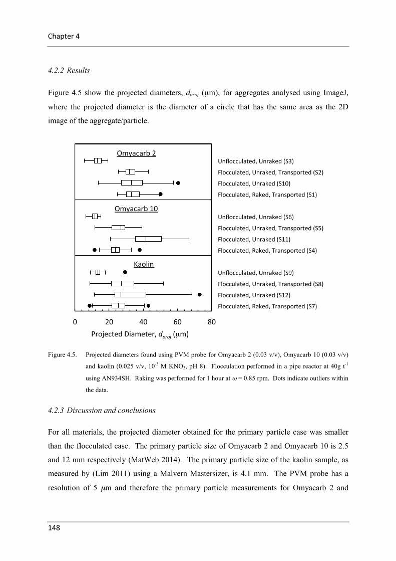
Chapter4

148

4.2.2 Results

Figure 4.5 show the projected diameters, dproj (µm), for aggregates analysed using ImageJ,

where the projected diameter is the diameter of a circle that has the same area as the 2D

image of the aggregate/particle.

Figure 4.5. Projected diameters found using PVM probe for Omyacarb 2 (0.03 v/v), Omyacarb 10 (0.03 v/v)

and kaolin (0.025 v/v, 10-3 M KNO3, pH 8). Flocculation performed in a pipe reactor at 40g t-1

using AN934SH. Raking was performed for 1 hour at ω = 0.85 rpm. Dots indicate outliers within

the data.

4.2.3 Discussion and conclusions

For all materials, the projected diameter obtained for the primary particle case was smaller

than the flocculated case. The primary particle size of Omyacarb 2 and Omyacarb 10 is 2.5

and 12 mm respectively (MatWeb 2014). The primary particle size of the kaolin sample, as

measured by (Lim 2011) using a Malvern Mastersizer, is 4.1 mm. The PVM probe has a

resolution of 5 µm and therefore the primary particle measurements for Omyacarb 2 and

0 20 40 60 80

Unflocculated,Unraked(S3)

Flocculated,Unraked,Transported(S2)

Flocculated,Unraked(S10)

Flocculated,Raked,Transported(S1)









ProjectedDiameter,dproj(µm)

Omyacarb2

Omyacarb10

Kaolin

RakedBatchSettling

149

kaolin are nonsensical and thus disregarded. A median particle size of 11.6 µm was obtained

for Omyacarb 10, which is around the expected value of 12 µm (MatWeb 2014).

For all materials tested, the sample flocculated just prior to using the PVM, (Samples 10, 11

and 12) resulted in a greater median particle size and standard deviations compared to the

sample flocculated at The University of Melbourne and transported (Samples 2, 5 and 8).

This indicates that the transport between facilities affected the samples by the addition of

shear through unwanted vibrations. Due to this, further discussions of results ignore samples

2, 5 and 8.

Comparing the raked samples (1, 4, and 7) to unraked samples (10, 11, and 12) shows an

overall slight decrease in median particle size. A reduction in the standard deviation is also

observed. This agrees with aggregate densification whereby raking causes a reduction in

aggregate diameter.

Only limited data was obtained and a number of key issues were not addressed, including:

• Shear on the aggregates during transport and handling from the raked column to the

PVM measurement system was not ideal.

• Data analysis is completely manual and hence time consuming. Development of an

automated system via macros is recommended.

Based on the limitations and key issues of this experiment, values obtained for aggregate

diameter cannot be used to specify aggregate diameter as a function of shear. However, the

trends in the data indicate the expected reduction in aggregate diameter when exposed to

shear.

4.3 Stationary Rake

Current raked batch settling test data analysis requires that the experimentalist first conduct

an un-raked settling test to determine material properties such as Py(φ) and R(φ). Previously,

unraked experiments of this type had assumed (untested) the presence of the rake would be

minimal. Other authors have indicated that the presence of a large rod, or other similar

Chapter4

150

object, can influence the settling rate (Buratto et al. 2014). Experiments were performed to

determine if in fact the presence of a stationary rake alters the settling rate and/or aggregate

densification. Table 4-2 outlines the operating conditions used for this work.

Table 4-2: Operating conditions for the determination of the effect of a stationary rake on batch settling.

Operating Conditions Initial solids volume fraction φ0 (v/v) 0.03 Flocculant dosage D (g t-1) 40 Initial settling height h0 (m) 0.3 Rake rotation rate ω (rpm) 0

4.3.1 Analysis

Un-raked settling tests were analysed using classical settling techniques, (de Kretser et al.

2001, Usher et al. 2001, Lester et al. 2005), to obtain standard dewatering material properties

such as hindered settling function, R(φ), compressive yield stress, Py(φ) and gel point, φg.

The theory and method for characterising fundamental dewatering material properties from

batch settling and pressure filtration experiments were presented in section 2.5.

4.3.2 Results

Measured transient and equilibrium height data were recorded for the batch settling tests and

are presented in Figure 4.6. The height data shows that the presence of a stationary rake

slightly decreases the initial rate of settling without significant variations in the final bed

height. The decrease in initial settling rate is expected due to the slight reduction in volume

available for the aggregates to settle, causing a greater drag. The insignificant variation in

final bed height indicates little variation in the extent of aggregate densification and hence

there are few, if any, interactions between the stationary rake and aggregates that cause

aggregate densification.

RakedBatchSettling

151

Figure 4.6: Transient interface settling height for the settling of flocculated (40 g t-1 AN934SH) calcite

(Omyacarb 2, φ0 = 0.03 v/v) with and without a stationary rake.

Figure 4.7 and Figure 4.8 display the difference in material properties between batch settling

with and without a stationary rake. As expected from the trends in the transient height data,

only a minor difference is observed in the functional forms of both the compressive yield

stress and hindered settling function.

0

0.05

0.1

0.15

0.2

0.25

0.3

1 10 100 1000 10000 100000 1000000

Hei

ght,

h (m

)

Time, t (s)

Rake 1 Rake 2 No Rake 1 No Rake 2

Chapter4

152

Figure 4.7: Compressive Yield Stress, Py(φ) as a function of solids concentration, φ, for flocculated

(AN934SH at 40 g t-1) calcite (Omyacarb 2, φ0 = 0.03 v/v) determined via batch settling tests with

and without a stationary rake present.

0.001

0.01

0.1

1

0.15 0.2 0.25 0.3 0.35

Com

pres

sive

Yie

ld S

tress

, Py(φ)

(kP

a)


No Rake Stationary Rake

RakedBatchSettling

153

Figure 4.8: Hindered settling, R(φ) as a function of solids concentration, φ, for flocculated (AN934SH at 40

g t-1) calcite (Omyacarb 2, φ0 = 0.03 v/v) determined via batch settling tests, with and without a

stationary rake present.

Table 4-3 shows the quantification of the difference in trends in the material properties

between the tests, with and without a stationary rake. Quantification of the deviation in

material properties due to the presence of a stationary rake is given by

, (4.3)

where SRave is the stationary rake average and NRave is the no rake average. Due to the use of

the same set of high-pressure filtration data, it is expected that the material properties

converge at higher solids volume fractions.

1.E+07

1.E+08

1.E+09

0.03 0.04 0.05 0.06 0.07 0.08

Hin

dere

d S

ettli

ng F

unct

ion,

R(φ

) (k

g s-

1 m-3

)


No Rake 1

No Rake 2

Stationary Rake 1

Stationary Rake 2

%100% ×−

=ave

aveave

NRSRNR

Error

Chapter4

154

Table 4-3: Comparison of dewatering extent due to the presence of a stationary rake

Compressive Yield Stress, Py(φ) (Pa) Hindered Settling Function,

R(φ) (kg s-1 m-3)

φave, f φg φ @ 1Pa φ @ 1kPa R(φ0) (107) R(0.06) (108)

SR1 0.212 0.190 0.194 0.331 4.57 2.99 SR2 0.227 0.206 0.210 0.337 4.86 3.30

SRave 0.220 0.198 0.202 0.334 4.72 3.14

NR1 0.231 0.210 0.214 0.339 3.06 2.96 NR2 0.225 0.204 0.208 0.336 2.90 2.89

NRave. 0.228 0.207 0.211 0.338 2.98 2.92

Difference 0.009 0.009 0.009 0.004 1.74 0.22 % Error 3.730 4.348 4.214 1.161 58.38 % 7.53 %

Below in Section 4.4, experimental consistency was investigated to determine experimental

errors relating to reproducibility and consistency between each experimental run. The %

Errors calculated from these results (Table 4-5) is shown in Table 4-4.

Table 4-4: Experimental error relating to reproducibility and consistency between all unsheared settling tests

conducted within this thesis. % Error calculated using equation 4.3 and data presented in Table

4-5.

Compressive Yield Stress, Py(φ) (Pa) Hindered Settling Function,

R(φ) (kg s-1 m-3) φave, f φg φ @ 1Pa φ @ 1kPa R(φ0) R(0.06)

% Error 12.5 7.4 6.8 2.0 60 64

Comparison of table 4-3 and 4-4 shows the % Error obtained due to the presence of a

stationary rake fall within the experimental errors. Hence the variance observed in settling

data and material properties is not significant and the presence of a stationary rake within un-

raked settling tests is not required. To further this point, equilibrium data analysis of raked

settling tests was completed using both sets of material properties. The results show a 0.8%

error in the final scaled aggregate diameter, Dagg,∞. Again, this value falls within the

expected error due to experimental reproducibility.

RakedBatchSettling

155

4.4 Experimental Consistency

All experiments were performed under the same conditions except for the one variable that

was under investigation. Variables manipulated are listed in section 4.1.4. To evaluate

consistency and flocculation reproducibility, an un-sheared settling test was performed with

every experiment. Assessment of consistency and flocculation reproducibility is now

presented.

4.4.1 Analysis





batch settling and pressure filtration experiments were presented in section 2.5.

4.4.2 Results

Fundamental dewatering material properties, R(φ) and Py(φ), for all the un-sheared settling

tests are shown in Figure 4.9 and Figure 4.10. As expected, slight variations in the material

properties exist between experiments due to reproducibility issues relating to flocculating a

particulate suspension. Table 4-5 quantifies differences in the material properties between

experiments. Due to the use of the same set of high pressure filtration data, it is expected that

the compressive yield stress converge at higher solids volume fractions. The results indicate

reasonable consistency was maintained throughout the experimental program.

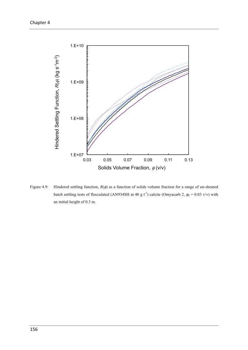
Chapter4

156

Figure 4.9: Hindered settling function, R(φ) as a function of solids volume fraction for a range of un-sheared

batch settling tests of flocculated (AN934SH at 40 g t-1) calcite (Omyacarb 2, φ0 = 0.03 v/v) with

an initial height of 0.3 m.

1.E+07

1.E+08

1.E+09

1.E+10

0.03 0.05 0.07 0.09 0.11 0.13

Hin

dere

d S

ettli

ng F

unct

ion,

R(φ

) (kg

s-1

m-3

)


RakedBatchSettling

157

Figure 4.10: Compressive yield stress, Py(φ), as a function of solids volume fraction for a range of un-sheared

batch settling tests of flocculated (AN934SH at 40 g t-1) calcite (Omyacarb 2, φ0 = 0.03 v/v) with

an initial height of 0.3 m.

0.001

0.01

0.1

1

0.15 0.2 0.25 0.3

Com

pres

sive

Yie

ld S

tress

, Py(φ)

(kP

a)


Chapter4

158

Table 4-5: Summary of hindered settling function and compressive yield stress variations between a series of

un-sheared settling tests performed. Measures of variation include; Py(φ) values at 1 Pa and 1

kPa, final average solids concentration, φf,ave solids gel point, φg, and R(φ) values at the initial and

twice the initial solids concentration.

Test R(φ0)

(kg s-1 m-3) (107)

R(0.06) (kg s-1 m-3)

(108) φf,ave φg φ @ 1Pa φ @ 1kPa

1 1.19 1.05 0.217 0.194 0.199 0.303 2 1.61 1.54 0.218 0.195 0.198 0.303 3 1.93 1.79 0.210 0.187 0.193 0.302 4 2.60 2.95 0.217 0.194 0.199 0.303 5 1.97 1.58 0.219 0.196 0.201 0.302 6 2.99 2.32 0.229 0.196 0.200 0.298 7 1.61 1.98 0.238 0.194 0.197 0.303 8 1.61 1.70 0.240 0.202 0.207 0.304

Mean, µ 1.94 1.86 0.224 0.195 0.199 0.302 Standard Deviation, σ 0.59 0.57 0.011 0.004 0.004 0.002

4.5 Standard Raked Settling

A series of standard sheared settling tests were performed to investigate the influence of

experimental variables such as shear rate (rake rotation rate), raking duration, flocculant

dosage, and initial settling height. For all settling tests presented within this section, raking

commences as the settling test commences, tstart = 0. Settling tests where raking commenced

once the majority of aggregates had settled, are presented in section 4.7.

The expected trends between aggregate densification parameters, A and Dagg,∞, and

experimental conditions for standard sheared settling tests is described below.

4.5.1 Expected trends

4.5.1.1 Rotation rate

Aggregate densification is the dewatering enhancement due to shear imparted on aggregates.

Hence, rake rotation rate, ω, is directly proportional to shear rate and therefore the rate

parameter for aggregate densification, A, is expected to be a strong function of rake rotation

rate, ω. As shear rates are increased, there becomes a point in which the excessive shear

causes aggregate breakage. Competing effects between densification and breakage is

RakedBatchSettling

159

expected to create an optimum shear rate with respect to A, with a corresponding critical rake

rotation rate.

The equilibrium scaled aggregate diameter, Dagg,∞, is proportional to the rate parameter for

densification multiplied by the raking time, A.t. Providing the raking duration is sufficient,

Dagg,∞ is likely to be independent of rake rotation rate. The time required to achieve Dagg,∞

therefore is a function of rake rotation rate and inversely proportional to A.

4.5.1.2 Initial height

Increasing the initial height results in an increase in the time an aggregate spends within the

sedimentation zone and an increase in the final bed height. Dewatering within the suspension

bed is limited by the rate in which the water can escape (flux limited). Dewatering is not flux

limited during sedimentation and hence, increasing the time within this zone is expected to

positively affect the rate of densification. With increased suspension bed, compressive forces

increase, resulting in an increased average solids concentration and yield stress. The pressure

the rakes apply onto aggregates is a strong function of the yield stress of the suspension

(Spehar 2014), resulting in an increase in both the extent and rate of densification with

suspension bed height.

Wall effects are expected to be increased with increasing initial settling heights. Lester and

Buscall (2015) showed an increase in the observed compressive yield stress with decreasing

bed heights and cylinder diameters. The relation between Dagg,∞and initial settling height is

governed by the competing effects of wall adhesion and yield stress driven dewatering.

4.5.1.3 Flocculant dose

The number of polymer molecules per volume of suspension increases with increasing

flocculant dosage. As a result, increasing flocculant dose results in an increase in formation

of particle bonds and the overall strength of the aggregate also increases. The ability to

densify aggregates through shear is largely dependent on the strength of the aggregate. The

stronger the aggregate the larger the force required overcoming the bonds and causing


Chapter4

160

Aggregate densification is the result of shear rearranging aggregates such that inter-aggregate

liquid is removed, reducing the overall size of the aggregate, and increasing the aggregate

settling rate. As individual (un-aggregated) particles are relatively incompressible compared

to flocculated aggregates, shearing an un-flocculated suspension is expected to result in no

aggregate densification and therefore no shear enhanced dewatering.

Therefore an optimum flocculation dose is expected to occur such that the corresponding

optimum aggregate strength results in a maximum rate and extent of aggregate densification.

Often, an optimum flocculant dose exists whereby the settling rate is maximised while

majority of particles are captured (La Mer and Healy 1963). Optimising the flocculant dose

with respect to aggregate densification parameters should also consider the effect on settling

rates and capture of fine particles.

4.5.2 Analysis





batch settling and pressure filtration experiments was presented in section 2.5

Combining the material properties obtained from un-raked settling tests, with transient and

equilibrium raked settling data allows for the determination of the rate, Α (s-1), and extent,

Dagg,∞, parameters describing aggregate densification. Analysis of sheared settling tests to

extract aggregate densification parameters was outlined in section 2.7.5.


Calcite (Omyacarb 2) was prepared at a solids concentration of 0.03 v/v and flocculated.

Suspension and polymer preparation along with subsequent flocculation was performed as

stated in section 4.1. The suspension and flocculant flow rates were adjusted to give the

desired flocculant dosage. Once flocculated, the calcite suspension was transferred into

settling cylinders up to the desired initial settling height. The raking apparatus was turned on

RakedBatchSettling

161

to commence raking as soon as all cylinders were filled. Raking continued for 72 hours

during which, the sediment interface height as a function of time was recorded. Table 4-6

summarises the operating conditions.

Table 4-6: Operating conditions for a series of batch settling tests investigating the effect of initial settling

height, flocculant dose, rake rotation rate and rake start and stop times on aggregate densification

parameters.

Operating Conditions: Base Variation Initial solids volume fraction φ0 (v/v) 0.03 - Initial settling height h0 (m) 0.3 0.6, 0.9, 1.2 Flocculant dose D (g t-1) 40 0, 80 Rake rotation rate ω (rpm) 0.2 0, 0.1, 4.2 Rake start time tstart (hr) 0 - Rake stop time tstop (hr) 72 -

4.5.4 Results: Base conditions

The base conditions, as defined in section 4.1.4 and Table 4-6, refers to the settling of

Omyacarb 2 flocculated at 40 g t-1 with an initial suspension solids concentration, φ0, of 0.03

v/v. This reference settling test had an initial settling height of 0.3 m and was raked at 0.2

rpm until equilibrium was obtained.

Transient sediment interface height data for the reference settling tests, both sheared and un-

sheared, are shown in Figure 4.11. The sheared settling test shows a clear dewatering

enhancement compared to the un-sheared case. It settles faster and further.

Chapter4

162

Figure 4.11: Sediment interface height, h(t) for sheared (ω = 0.21 rpm) and un-sheared batch settling tests of

flocculated (AN934SH at 40 g t-1) calcite (Omyacarb 2, φ0 = 0.03 v/v) with an initial height of

0.3 m.

Un-sheared settling tests resulted in a final bed height of 0.050 m, giving rise to an average

final solids concentration of 0.158 v/v. Using these values, high pressure filtration data and

equation 2.46, an optimised curve fit was obtained for the compressive yield stress, Py0(φ),

using a constitutive equation described by equation 2.24. The un-sheared, Py,0(φ), curve

fitting parameter values obtained for φg,0, a0, b, k0 and φcp were 0.188, 0.80, 0.01, 5.52 and

0.63 respectively. Using the un-sheared compressive yield stress curve and the equilibrium

bed height for the sheared test, 0.027m, the final extent of aggregate densification was Dagg,∞

= 0.88 and the final gel point, φg∞ = 0.280. These values are summarised in Table 4-7.

0

0.05

0.1

0.15

0.2

0.25

0.3

1 10 100 1000 10000

Height,h(m

)

Time,t(s)

Unraked

Raked,0.21rpm

RakedBatchSettling

163

Table 4-7: Equilibrium bed height data for un-sheared and sheared (0.21 rpm) Omyacarb 2 settling data

flocculated at 40 g t-1 (AN934SH) with an initial settling height of 0.3 m.

h0 (m)

hf (m)

φ0 (v/v)

φf,ave (v/v)

φg,0 (v/v)

φg,∞ (v/v)

Dagg∞ (-)

Unsheared 0.263 0.050 0.030 0.158 0.188 1 Sheared 0.263 0.027 0.030 0.219 0.280 0.88

An optimised curve fit was obtained for the compressive yield stress of the sheared

suspension, Py(φ,Dagg∞) though solving equation 2.81 and utilising the values obtained for

Py,0(φ). The sheared Py(φ, Dagg∞) curve fitting parameter values obtained for φg, a1, b, k1 and

φcp were determined to be 0.280, 0.75, 0.01, 5.39 and 0.63 respectively. Py(φ,Dagg∞) and

Py,0(φ) are presented in Figure 4.12 along with the pressure filtration data.

Figure 4.12: Compressive yield stress, Py(φ) as a function of solids volume fraction for un-densified (Dagg = 1)

and densified (Dagg = Dagg,∞ = 0.88) batch settling tests of flocculated (AN934SH at 40 g t-1)

calcite (Omyacarb 2, φ0 = 0.03 v/v) with an initial height of 0.3 m.

0.01

0.1

1

10

100

0 0.1 0.2 0.3 0.4 0.5

Com

pres

sive

Yie

ld S

tress

, Py(φ)

(kP

a)


Dagg = 1

Dagg = 1

Dagg = 0.75

Filtration Data Dagg = 1 Dagg,∞ = 0.88

Chapter4

164

The un-sheared hindered settling function, R0(φ), was determined and is shown in Figure

4.13. Using equations 2.71 – 2.73 and Dagg,∞ = 0.88, the hindered settling function for the

sheared reference, R(φ,Dagg,∞), is also shown in Figure 4.13.

Figure 4.13: Hindered settling function, R(φ) as a function of solids volume fraction for un-densified (Dagg = 1)

and densified (Dagg = Dagg,∞ = 0.88) batch settling tests of flocculated (AN934SH at 40 g t-1)

calcite (Omyacarb 2, φ0 = 0.03 v/v) with an initial height of 0.3 m.

Figure 4.14 shows the mean proportional error for the reference sheared settling test,

calculated via equation 2.82, as the densification rate parameter is varied. Upon refinement,

the optimum densification rate parameter, A, was determined to be 1.32 x 10-3 s-1 with a mean

proportional error, Ē, of 0.114.

Using the modified Kynch method, the optimised fit of the interface height, using Dagg∞ =

0.88 and A = 1.32 x 10-3 s-1, is shown in Figure 4.15. The predicted settling curve is of

reasonable accuracy, however, it under-predicts the interface height at early times and over-

1.E+05

1.E+06

1.E+07

1.E+08

1.E+09

1.E+10

1.E+11

1.E+12

0 0.1 0.2 0.3 0.4 0.5

Hin

dere

d S

ettli

ng F

unct

ion,

R(φ

) (kg

s-1

m-3

)


Dagg = 1 Dagg = 0.75 Dagg = 1

Dagg = 1

Dagg,∞ = 0.88

Data points

RakedBatchSettling

165

predicts at later times. For the case presented, this transition occurs after 710 seconds (height

of 0.065 m). This trend is commonly observed in the majority of the following experimental

analysis within this thesis and by previous authors (van Deventer 2012). Although not

performed herein, this trend indicates that the use of a variable rate parameter (for example a

solids concentration dependence) could yield a more accurate prediction.

Figure 4.14: Mean proportional error in time versus the densification rate parameter, A, calculated for the

optimisation of the predicted interface height against experimental data for the sheared (ω = 0.21

rpm) settling of flocculated (40g t-1 AN934SH) calcite (Omyacarb 2, φ0 0.03 v/v)

0.1

1

0 0.002 0.004 0.006 0.008 0.01

Mea

n P

ropo

rtion

al E

rror

, Ē

Densification Rate Parameter, A (s-1)

Chapter4

166

Figure 4.15: Predicted sediment interface height, h(t), curve fit incorporating aggregate densification using the

optimum value of A (0.00135 s-1). Predicted and experimental data represents batch settling tests

of flocculated (AN934SH at 40 g t-1) calcite (Omyacarb 2, φ0 = 0.03 v/v) with an initial height of

0.3 m.

4.5.5 Results: Rake rotation rate

Raked sedimentation tests were conducted to quantify the effect of shear rate (through rake

rotation rate, ω, on the rate and extent of aggregate densification. Experiments were at the

base conditions except the rake rotation rate, which varied between 0 and 8.36 rpm.

Normalised transient interface height data is shown in Figure 4.16. For clarity, only

experimental data at rotation rates of 0, 0.21, 2.09, 4.2 and 8.63 rpm are shown. Settling tests

at 11 other rotation rates were also performed however, yielded similar results and trends. A

full summary of settling tests with variable rake rotation rate is shown in Table 4-8. A clear

enhancement in dewatering due to shearing when compared to the un-sheared transient

0

0.05

0.1

0.15

0.2

0.25

0.3

1 10 100 1000 10000

Hei

ght,

h (m

)

Time, t (s)

Sheared Sedimentation

Predicted Settling

RakedBatchSettling

167

settling data was observed. The determined aggregate densification parameters as functions

of rake rotation rate, A(ω) and Dagg,∞ (ω), are shown in Figure 4.17 and Figure 4.18 and

summarised in Table 4-8.

Figure 4.16: Normalised sediment interface height, H(t) for batch settling tests of flocculated (AN934SH at

40 g t-1) calcite (Omyacarb 2, φ0 = 0.03 v/v) with an initial height of 0.3 m and sheared at rotation

rates, ω, of 0, 0.21, 2.09, 4.2 and 8.63 rpm. Data at other rotation rates were omitted for clarity.

0

0.1

0.2

0.3

0.4

0.5

0.6

0.7

0.8

0.9

1

1 10 100 1000

Nor

mal

ised

hei

ght,

H

Time, t (s)

0rpm

0.21rpm

2.09rpm

4.2rpm

8.63rpm

Chapter4

168

Figure 4.17: Extent of aggregate densification as a function of rotation rate, ω, for flocculated (AN934SH at

40 g t-1) calcite (Omyacarb 2, φ0 = 0.03 v/v) with an initial settling height of 0.3 m. The results

are combined from three sets of data.

0.8

0.82

0.84

0.86

0.88

0.9

0.92

0.94

0.96

0.98

1

0.01 0.1 1 10 100

Scaled

AggregateDiameter,D

agg∞

RakeRoatanonRate,ω(rpm)

Average

RakedBatchSettling

169

Table 4-8. Extent of aggregate densification, Dagg, ∞, initial and final gel points, φg,o & φg,∞, at various rotation

rates, ω, for flocculated (AN934SH at 40 g t-1) calcite (Omyacarb 2, φ0 = 0.03 v/v) with an initial

settling height of 0.3 m. Raking was for 72 hr.

ω (rpm)

h0 (m)

hf (m)

ϕf

ϕg,0

ϕg, ∞

Dagg,∞

A (x103 s-1)

0 0.263 0.050 0.158 0.187 - 1 - 0.037 0.317 0.031 0.307 0.295 0.85 0.03 0.076 0.303 0.029 0.313 0.303 0.85 0.08 0.152 0.311 0.031 0.301 0.289 0.87 0.10 0.170 0.262 0.026 0.299 0.291 0.86 4.06 0.210 0.263 0.027 0.296 0.280 0.87 1.35 0.340 0.261 0.026 0.307 0.290 0.86 4.56 0.420 0.266 0.025 0.314 0.309 0.85 0.95 0.620 0.264 0.026 0.300 0.294 0.86 1.00 0.700 0.263 0.026 0.298 0.293 0.86 14.50 0.860 0.254 0.024 0.314 0.308 0.85 1.70 1.240 0.283 0.029 0.297 0.281 0.87 1.20 2.090 0.268 0.026 0.314 0.299 0.86 7.50 2.550 0.281 0.029 0.291 0.278 0.88 1.05 4.19 0.262 0.025 0.314 0.304 0.85 0.69 4.20 0.285 0.028 0.302 0.294 0.86 3.20 8.630 0.265 0.026 0.306 0.295 0.86 1.62

Chapter4

170

Figure 4.18: Aggregate densification rate parameter, A, (s-1), as a function of rake rotation rate, ω, for

flocculated (AN934SH at 40 g t-1) calcite (Omyacarb 2, φ0 = 0.03 v/v) with an initial settling

height of 0.3 m. The data was extracted using the modified Kynch method to optimise predicted

settling curves (van Deventer et al. (2011)).

The final scaled aggregate diameter, Dagg,∞, at different rake rotation rates varied between

0.85 and 0.88 and showed an average value of 0.86. The range is assumed to represent the

experimental error in this system. The extent of aggregate densification is observed to be

independent of shear rate, providing the time of raking is sufficient such that Dagg,∞ can be

obtained. The raking time required to obtain Dagg,∞ depends on the rate of aggregate

densification according to equation 2.61.

Α ranges from 3.5 x 10-5 s-1 (at 0.037 rpm) to 4.2 x 10-3 s-1 (at 0.17 rpm) and is clearly a

function of rake rotation rate, ω. At low rake rotation rates, Α slowly increases until it

reaches a critical rotation rate. Above this critical rotation rate, variation in Α becomes

0.00001

0.0001

0.001

0.01

0.01 0.1 1 10

RateParam

eterfo

rDen

sificano

n,A(s

-1)

RakeRotanonRate,ω(rpm)

Series1Curve Fit

RakedBatchSettling

171

scattered and weakly dependent on the rake rotation rate. For flocculated (AN934SH at 40 g

t-1) calcite (Omyacarb 2, φ0 = 0.03 v/v), this critical rotation rate is between 0.15 and 0.17

rpm.

Although the reason for the trend in the rate of aggregate densification with rotation rate is

unknown, it is thought to be the result of a minimum required force to cause permanent

deformation to the aggregates. Due to the distribution of aggregate size and strength, at low

rotation rates, the corresponding shear rate and rake pressure is sufficient to cause permanent

deform to only the weaker aggregates. As the rotation rate increases, the force increases and

more and more aggregates are able to be permanently deformed. Beyond the critical rotation

rate, the shear rate and rake pressure is sufficient to cause permanent deformation to the

majority of the aggregates. Further increase in rotation rate provides the ability to

permanently deform the stronger aggregates however aggregate breakage occurs resulting in

a plateau region. Further work investigating this trend is highly recommended.

Based on the data obtained, a curve fit was applied to the data to obtain a hypothetical

aggregate densification rate parameter as a function of rake rotation rate. The functional

form of the curve fits that are depicted in Figure 4.18 is given by,

( )⎭⎬⎫

≥

<≤

⎩⎨⎧

×

×=

−

−

16.016.00

1068.17

1086.7 4

4

ω

ωωωA . (4.4)

Incorporation of the relation between the average maximum shear rate and rake rotation rate,

equation 4.1, results in A( maxγ! ) given by,

( )⎭⎬⎫

≥

<≤

⎩⎨⎧

×

×=

−

−

096.0096.00

1061.10

1072.4

max

max4max

4

max γ

γγγ

!!!

!A . (4.5)

Equation 4.4 and 4.5 describes A as a linear function of ω (or γ) below a critical value and

independent of ω (or γ) above this critical value. Difficulties arose for experiments at low

rotation rates due to the increased potential for compromised experimental data to be

obtained. For example, due to the low shear rates; minimal bumps/vibrations to the raking

apparatus can cause further densification that cannot be separated from densification due to

Chapter4

172

raking. Providing these issues can be overcome, it is highly recommended to perform

experiments at rotation rates below the critical value to enable a proper statistical analysis and

draw conclusions regarding the relationship between A and ω (or γ).

Equation 4.4 and 4.5 models the rate of aggregate densification as undergoing a step change

at the critical rotation rate. This is not expected to be the case according to the proposed

theory above. Due to the lack of data below the critical rotation rate, a step change is

currently the best option in order to provide an equation describing the effect of rotation rate

on the densification rate parameter. Use of equations 4.4 and 4.5 around the critical value

should be avoided until further experiments are performed and the trend further defined.

Once breakage completely dominates over densification, the transient interface height

approaches that of an un-flocculated suspension. Compromised experimental data is obtained

at such high rotation rates where breakage completely dominates due to experimental

restrictions. For example, the raking apparatus vibrated and caused a range of other issues

that could not be separated from densification effects.

The data for Omyacarb 2 flocculated at 40 g t-1 implies that a shear rate corresponding at least

0.16 rpm (shear rate of 0.096 s-1) provides optimal dewatering enhancement due to aggregate

densification. It is believed that this critical shear value corresponds to the minimum

requirement for particles to collide such that below this value, natural aggregate kinetics

allow for them to move out of the way.

4.5.6 Results: Initial height

Sheared and un-sheared settling tests were performed at initial settling heights of 0.6, 0.9, and

1.2 m to quantify the effect of initial settling height on dewatering enhancement due to


All previous batch settling tests were conducted with an initial settling height of 0.3 m

resulting in the aggregates having a maximum sedimentation residence time of 20 mins and

the equilibrium bed formed having a height of order 0.025 m. Previous studies showed little

variation and did not explain trends in the extent of aggregate densification with rake rotation

RakedBatchSettling

173

rate. Variations in the initial settling height are aimed at investigating this trend through

increased accuracy of equilibrium bed height measurements. Through increasing the initial

height, the effect of increased sedimentation time and yield stress on aggregate densification

was also probed.

Current equilibrium analysis utilises the initial and final bed heights to determine the

compressive yield stress, Py(φ), solids gel point, φg, and the extent of aggregate densification

as described in section 2.5.1.2. These three parameters are therefore heavily dependent on

the accuracy of the final bed height reading. It is therefore beneficial to consider the

accuracy of these measurements. For example, if the final bed height on the sheared and un-

sheared reference were distorted by 1 mm the resultant φg and Dagg∞ would change by 4.3 %

and 1.5 % respectively. Increasing the initial height proportionally increases the final bed

height and therefore increases the accuracy of the equilibrium analysis.

4.5.6.1 Un-sheared

One concern with increasing the initial settling height is that wall effects start to reduce the

overall settling rate and compressive yield stress. Previous results have shown that wall

effects are significant in the majority of batch settling experiments, resulting in errors

associated with the estimation of the compressive yield stress of a strongly flocculated

suspension (Lester et al. 2013, Lester and Buscall 2015).

Transient interface height data obtained for un-sheared batch settling tests of flocculated

(AN934SH at 40 g t-1) calcite (Omyacarb 2, φ0 = 0.03 v/v) with initial heights of 0.26, 0.6,

0.9, and 1.2 m is shown in Figure 4.19. Fundamental dewatering material properties, R(φ),

Py(φ) and φg, have been obtained and presented in Figure 4.20 and Figure 4.21.

Quantification of the variation in material properties is presented in Table 4-9.

Chapter4

174

Figure 4.19: Sediment interface height, h(t) for un-sheared batch settling tests of flocculated (AN934SH at

40 g t-1) calcite (Omyacarb 2, φ0 = 0.03 v/v) with initial heights of 0.26, 0.6, 0.9 and 1.2 m.

0

0.2

0.4

0.6

0.8

1

1.2

1.4

1.E+00 1.E+01 1.E+02 1.E+03 1.E+04 1.E+05 1.E+06

Hei

ght,

h (m

)

Time, t (s)

0.26

0.6

0.9

1.2

h0 (m)

RakedBatchSettling

175

Figure 4.20: Hindered settling function, R(φ), as a function of solids concentration, φ (v/v), for the settling of

flocculated (40 g t-1 AN935SH) calcite (Omyacarb 2 at φ0 = 0.03 v/v) at various initial settling

heights. Solids concentration range has been restricted between φ0 = 0.03 v/v and the fan limit

solids concentration, φfl = 0.13 v/v.

1.E+07

1.E+08

1.E+09

1.E+10

0.03 0.05 0.07 0.09 0.11 0.13

Hin

dere

d S

ettli

ng F

unct

ion,

R

(φ) (

kg s

-1 m

-3)


0.26

0.6

0.9

1.2

h0 (m)

Chapter4

176

Figure 4.21: Compressive yield stress, Py(φ), as a function of solids concentration, φ (v/v), for the settling of

flocculated (40 g t-1 AN935SH) calcite (Omyacarb 2 at φ0 = 0.03 v/v) at various initial settling

heights.

Table 4-9: Material property analysis for different initial settling heights using flocculated (40 g t-1

AN935SH) calcite (Omyacarb 2 at φ0 = 0.03 v/v) data. Measures of variation include; Py(φ)

values at 1 Pa and 1 kPa, final average solids concentration, φf,ave, solids gel point, φg, and R(φ)

values at the initial and twice the initial solids concentration.

h0 (m)

hf (m)

φf.ave (v/v)

φg (v/v)

R(φ0) (kg s-1 m-3)

(x107)

R(2φ0) (kg s-1 m-3)

(x107)

φ @ 1Pa (v/v)

(x103)

φ @ 1kPa (v/v)

0.260 0.034 0.229 0.187 1.971 18.272 0.192 0.302 0.600 0.072 0.252 0.232 1.732 16.699 0.236 0.305 0.913 0.107 0.257 0.234 1.969 17.889 0.237 0.297 1.226 0.137 0.268 0.245 1.598 16.148 0.248 0.297

Mean, µ 1.818 17.252 0.228 0.300 Standard Deviation, σ 0.184 0.995 0.025 0.004

0.01

0.1

1

10

100

0 0.1 0.2 0.3 0.4 0.5

Com

pres

sive

Yie

ld S

tress

, Py(φ)

(kP

a)

Solids Concentration, φ (v/v)

0.26

0.6

0.9

1.2

FiltranonData

h0 (m)

RakedBatchSettling

177

Comparison of the hindered settling function is restricted to the solids concentration range

from the initial solids concentration, φ0 = 0.03 v/v, to the fan limit, φfl = 0.13 v/v. The

analysis method used to determine R(φ) extrapolates for values beyond these solids

concentrations. Minimal variation in R(φ) is observed between these limits with variations

within expected experimental consistency. Therefore it is concluded that the initial settling

height has no impact on the determination of the hindered settling function.

Little variation in the compressive yield stress is experienced at solids concentrations above

0.3 v/v, corresponding to a compressive yield stress Py(0.3) = 1 kPa. At solids concentrations

below this, significant variations in Py(φ) exist. This is highlighted by the gel point, which

increases with increasing initial heights from 0.187 to 0.245 v/v. The reason for significant

discrepancies between compressive yield stresses for various initial heights at low solids

concentration is unknown.

4.5.6.2 Sheared

A sheared sedimentation test was conducted to investigate the effect of initial height on the

rate and extent of aggregate densification. The following settling test was performed at the

base conditions (φ0 = 0.03 v/v, D = 40 g t-1, ω = 0.2 rpm) except for the initial settling height,

h0 = 1.2 m.

The normalized sediment-liquid interface height versus time data is shown in Figure 4.22 for

both un-sheared and sheared sedimentation tests at initial heights of 0.26 and 1.22 m. The

sheared case shows a clear performance enhancement over the un-sheared case. Standard

densification analysis was performed on the settling data, with the resultant aggregate

densification parameters presented in Table 4-10.

Chapter4

178

Figure 4.22: Normalised transient interface height, H(t) for the settling for flocculated (40 g t-1) Omyacarb 2

(φ0 0.03 v/v) un-sheared and sheared (ω = 0.21 rpm) for initial heights of 0.26 and 1.22 m.

Table 4-10. Final scaled aggregate diameter, Dagg,∞, initial and final gel points, φg,0, φg,∞, for flocculated (40

g t-1) Omyacarb 2 (φ0 0.03 v/v) un-sheared and sheared (ω = 0.21 rpm) for initial heights of 0.26

and 1.22 m.

h0 (m)

ω (rpm)

hf (m)

φ0 (v/v)

φf (v/v)

φg,0 (v/v)

φg,∞ (v/v)

Dagg,∞

A (x103) (s-1)

0.263 0 0.050 0.03 0.158 0.187 - 1 0 1.226 0 0.137 0.03 0.268 0.245 - 1 0 0.263 0.2 0.027 0.03 0.296 - 0.280 0.88 1.32 1.211 0.2 0.109 0.03 0.333 - 0.316 0.85 0.96

The resultant aggregate densification rate parameter for an initial settling height of 1.2 m is of

similar order as the result for an initial settling height of 0.3 m and agrees with the trends

observed in section 4.5.5. The equilibrium scaled aggregate diameter however, is slightly

0

0.1

0.2

0.3

0.4

0.5

0.6

0.7

0.8

0.9

1

0 2000 4000 6000 8000

Nor

mal

ised

hei

ght,

H

Time, t (s)

Raked Unraked

h0 (m) 0.26 1.22

RakedBatchSettling

179

less for the initial settling height of 1.2 m compared against the 0.3 m case. It is believed that

the following contribute to the observed difference in Dagg,∞;

• External disturbances and vibrations due to the practicality of performing a batch

settling test with an initial height of 1.2 m.

• As initial height increases, batch settling tests become more susceptible to mixing

with height and the assumption of line settling, inherent within the material properties

no longer applies.

• The yield stress of the suspension bed causes rake deformation, which is more

prevalent for longer rakes.

• A 1.2 m settling column, at the experimental suspension flow rate, has a fill time of

order 60 seconds. As a result a uniform initial solids concentration is not present.

Modifications to the suspension flow rate to reduce the fill time are impractical as it

results in extra shear during flocculation. Re-homgenisation is also unreasonable as

this in itself involves applying extra shear.

The data presented is insufficient to adequately describe the trends between aggregate

densification parameters and initial height. Although not performed herein, the data suggests

sheared settling tests at a range of initial heights be conducted to further investigate the trend

between initial settling height and aggregate densification parameters. An alternative of

fluidisation could also be applied.

4.5.7 Results: Flocculant dosage

A series of sheared batch settling tests were performed at flocculant doses of 0, 40 and

80 g t-1 to investigate the effect of over and under dosing on the dewatering performance

enhancement achieved due to aggregate densification. The effect of over and under dosing

was also investigated for un-sheared settling tests at these doses. The resultant transient

settling data is shown in Figure 4.23.

It should be noted that floc size or density measurements were not performed in this work,

although by visual observations, floc size considerably increased with flocculant dosage.

Chapter4

180

Figure 4.23: Normalised transient height, H(t), for sheared and un-sheared settling tests of calcite (Omyacarb 2

at 0.03 v/v) flocculated with AN934SH at 0, 40 and 80 g t-1. The sheared settling tests were raked

at a rotation rate of 0.2 rpm until dewatering effectively ceased (72 hr).

No variation is observed between the un-flocculated (0 g t-1) sheared and un-sheared settling

data indicating that raking seems to have no effect on non-flocculated (un-aggregated)

slurries. The individual (un-aggregated) particles are incompressible compared to flocculated

aggregates and dewatering enhancement due to shearing is not expected. No variation in the

rate of settling indicates that raking during settling does not create any material hold up or

negative settling effects. Insignificant variations in the un-flocculated settling data at large

times indicates that the creation of channels behind the rakes allowing for liquor to escape,

has little to no enhancement in dewatering of the sediment bed.

Conversely, the sheared 80 g t-1 settling test experienced a slower settling rate compared to

the un-sheared test and as a consequence, an aggregate densification rate parameter was not

0

0.1

0.2

0.3

0.4

0.5

0.6

0.7

0.8

0.9

1

1 10 100 1000 10000

Nor

mal

ised

hei

ght,

H

Time, t (s)

0 g t-1, Sheared 40 g t-1, Sheared 80 g t-1, Sheared 0 g t-1, Unsheared 40 g t-1, Unsheared 80 g t-1, Unsheared

RakedBatchSettling

181

obtained. One explanation for this decrease in settling rate is due to over dosing where

excess polymer within the system causes brief attachment of the aggregates to the rake.

Alternatively, the aggregates are sufficiently large such that aggregate flow around the rakes

cannot be achieved and instead the rakes tear and stretch the aggregates causing breakage.

An increase in the extent of aggregate densification was still observed with Dagg,∞ = 0.82 and

an increase in the gel point, φg, of Δφg = 0.09 v/v.

Another source of error is due to the experimental procedure; in which flocculation occurs

within a pipe reactor and aggregates are subsequently transferred to a settling cylinder. The

time scale for filling the settling cylinders to an initial height of 0.3 m is between 10 and 20

seconds. For the 80 g t-1 settling tests, a significant proportion of the settling occurred within

the time scale of filling resulting in compromised data. All results from the 80 g t-1 settling

tests are compromised and therefore have been discarded.

Overall, the settling rate increases with flocculant dose due to the increase in aggregate size.

Due to each flocculant dosage having a different initial gel point, φg,0, comparison of the

change in gel point is used as a measure of the change in the extent of aggregate

densification. A change in gel point of 0, 0.093 and 0.090 v/v was observed for flocculant

dosages of 0, 40 and 80 g t-1 respectively. A summary of the equilibrium data is presented in

Table 4-11.

Table 4-11: Final extent of aggregate densification, Dagg,∞, initial and final gel points, φg0, φg,∞, for Omyacarb 2

(φ0 0.03 v/v), raked at 0. 2 rpm and flocculated at 0, 40 and 80 gt-1 of solids.

D (g t-1)

ω (rpm)

h0 (m)

hf (m)

ϕf,ave (v/v)

ϕg,0 (v/v)

ϕg, ∞ (v/v)

Dagg,∞

A (103 s-1)

0 0 0.261 0.017 0.461 0.212 - 1 - 0 0.2 0.258 0.017 0.461 - 0.212 1 0 40 0 0.238 0.034 0.158 0.187 - 1 - 40 0.2 0.263 0.027 0.292 - 0.280 0.87 1.35 80 0 0.258 0.057 0.136 0.114 - 1 - 80 0.2 0.258 0.036 0.214 - 0.204 0.82 NA

The data presented is insufficient to adequately describe the trends between aggregate

densification parameters and flocculant dosage. Although not performed herein, the data

suggests that further investigations of the effect flocculant dose be performed.

Chapter4

182

4.6 Shear during Sedimentation

In earlier experiments in which A(ω) and Dagg(ω) were investigated, raking was performed

until dewatering effectively ceased (approx. 7hr). This procedure is not useful in

understanding the individual contributions to dewatering either during sedimentation or

consolidation. Under the given experimental conditions, the majority of aggregates have

settled and are within the consolidating bed within 20 mins; hence results are closer related to

shear during consolidation. To understand the effect of shear during the sedimentation

regime, raking during was restricted, with a maximum duration of 20 mins.

4.6.1 Expected trends

Within the sedimentation zone during batch settling and thickening, the solids concentration

is sufficiently low such that open pathways are available between aggregates for water to

flow through and escape, not inhibiting dewatering of the suspension. Conversely, the time

an aggregate spends within the sedimentation zone of a thickener is often orders of magnitude

smaller than the residence time in the suspension bed.

Besides for the ability for water to escape, the rake torque is another limiting factor during

thickener operation. Rudman et al. (2008) showed the rake torque within a thickener can be

modelled as a linear function of the shear yield stress. Within the sedimentation zone, the

shear yield stress of the suspension is zero due as the solids concentration is below the gel

point. Therefore, raking during settling imparts less torque onto the rakes compared to raking

during compression, where the shear yield stress in non-zero.

Therefore, the overall residence time an aggregate can potentially be sheared for is orders of

magnitude less than within the suspension bed. For previous sheared batch settling tests, the

solids residence time during sedimentation was a maximum 20 mins compared to the overall

raking duration of 7 hr. The difference in solids residence time within either the

sedimentation or consolidation regime within a thickener is highlighted in Chapter 3 and

Chapter 5. Another shortcoming of shear during sedimentation arises due to the low solids

concentration, reducing aggregate-rake and aggregate-aggregate interactions. van Deventer

RakedBatchSettling

183

(2012) quantified this through a solids concentration dependency on the rate of aggregate

densification.

Due to the above rational, the expected relation between aggregate densification parameters

and sedimentation raking time is as follows;

• A is independent of raking duration for a constant rake rotation rate.

• Dagg,∞ scales with raking duration according to equation 2.61.

• Both A and Dagg,∞ obtained for shear during sedimentation is significantly less than

values obtained for shear during both sedimentation and consolidation and shear only

during consolidation.

4.6.2 Analysis





batch settling and pressure filtration experiments was presented in section 2.5.


equilibrium raked settling data allows for the determination of the densification rate

parameter, Α, and equilibrium scaled aggregate diameter, Dagg,∞. Analysis of sheared settling

tests to extract aggregate densification parameters was outlined in section 2.7.5. Settling

height prediction was performed using the implicit transient batch settling (TBS) model

modified to account for variations in tstop. TBS model theory was presented in section 2.8.

These results are the first in which the developed implicit TBS model was applied. Hence,

discussion regarding the accuracy and computational time is also presented.

Chapter4

184

4.6.2.1 Implicit model: Accuracy and computational time

The implicit scheme showed reasonable accuracy compared to the experimental data and had

the same order of magnitude errors when compared to both the explicit and semi-implicit

schemes. As the time step was increased for the implicit scheme, no notable differences in

the accuracy was observed, indicating that the use of a greater time step is practical.

Currently, the TBS model is implemented with a constant time step based on the Courant–

Friedrichs–Lewy (CFL) condition for the semi-implicit scheme given by equation 2.96. Due

to the increased number of equations to solve, the implicit scheme at the semi-implicit CFL

condition resulted in increased computational time. Theoretically, the implicit scheme is

numerically stable and convergent at any time step. At a time step greater than ~0.95s, the

implicit scheme failed.

Although an implicit scheme is theoretically always numerically stable and convergent, an

inherent constraint on the maximum allowable time step exists such that the material cannot

settle at a rate faster than one height element, j, per time step, Δt. Initially the sedimentation

rate is at a maximum and hence this constraint is particularly problematic at the start of the

simulation.

A proposed method to overcome this inherent time step constraint involves the

implementation of a variable time step. A scheme for this is currently not readily available

and it is suggested that an adhoc method of altering the time step based on the interface

height change is used. Implementation issues were encountered trying to incorporate a

variable time step and as such, all data analysis used either the semi-implicit scheme or the

new implicit scheme with a time step of 0.95s.


Calcite (Omyacarb 2) was prepared at solids concentration of 0.03 v/v and flocculated.

Suspension and polymer preparation along with subsequent flocculation was performed as

stated in section 4.1.4. The flocculated calcite suspension was transferred into settling

cylinders up to the initial settling height of 0.3 m. The raking apparatus was turned on to

RakedBatchSettling

185

commence raking as soon as all cylinders were filled. Raking continued for 3, 14, and 20

mins during which, the sediment interface height as a function of time was recorded. To

ensure the networked bed was unraked, the bottoms of the rakes were positioned 3 cm above

the base of the cylinder. The experiment used a rake rotation rate of 0.072 rpm, chosen to

ensure aggregate breakage was not significant. Table 4-12 summarises the operating

conditions used to investigate shear during sedimentation.

Table 4-12: Operating conditions for batch settling tests to determine aggregate densification parameters due

to shearing exclusively during sedimentation.

Operating Conditions: Base Variation Initial solids volume fraction φ0 (v/v) 0.03 - Initial settling height h0 (m) 0.3 - Flocculant dosage D (g/t) 40 - Rake rotation rate ω (rpm) 0.072 - Rake start time tstart (min) 0 - Rake stop time tstop (min) 20 0, 3, 14

4.6.4 Results

Normalised transient sediment interface height data for shear during sedimentation settling

tests at various raking durations are shown in Figure 4.24. Dewatering enhancement

compared to the un-sheared case cannot be observed from the transient sediment interface

data. A full summary of shear during sedimentation settling tests with variable raking

duration is summarised in Table 4-13 along with the calculated aggregate densification

parameters, A and Dagg,∞.

Results indicate no trends in both the rate and extent of aggregate densification with respect

to the raking duration. However, the analysis produces a rate parameter of 7 x 10-5 s-1 (a low

value in agreement with equation 4.4 and Dagg,∞ ranging between 0.92 and 0.96. These

values have been referenced within section 4.8 to compare raking during sedimentation and

consolidation.

Chapter4

186

Figure 4.24. Transient height versus time for raked settling tests of Omyacarb 2 at 0.03 v/v, flocculated with

AN934SH at 40 g t-1 conducted at a rotation rate of 0.072 rpm and various rake stop times, tstop =

179, 840 and 1300 s. Filled symbols indicate raked portion of the settling curve. Initial heights

range from 0.25 to 0.28 m.

Table 4-13. Final extent of aggregate densification, Dagg,∞, initial and final gel points, φg,0, φg,∞, for flocculated

Omyacarb 2 using 40 g t-1 of solids AN934SH, raked at 0.072 rpm and various rake stop time,

tstop.

tstop (s)

h0 (m)

hf (m)

φ0 (v/v)

φf (v/v)

φg,0 (v/v)

φg,∞ (v/v)

Dagg,∞

A (s-1)

0 0.263 0.050 0.03 0.158 0.187 - 1 - 179 0.277 0.033 0.03 0.252 0.236 0.93 7x10-5 840 0.262 0.034 0.03 0.231 0.213 0.96 7x10-5 1300 0.271 0.032 0.03 0.254 0.239 0.92 7x10-5

Sheared average 0.246 0.229 0.94 7x10-5

0

0.1

0.2

0.3

0.4

0.5

0.6

0.7

0.8

0.9

1

1.E+00 1.E+01 1.E+02 1.E+03 1.E+04 1.E+05 1.E+06

Nor

mal

ised

Hei

ght,

H

Time, t (s)

179s 840s 1300s

179s2 840s2 1300s2

tstop (s) Raked: 179 840 1300 Unraked: 179 840 1300

RakedBatchSettling

187

Due to the nature of the experiment, the raking duration (tstop – tstart) is representative of the

maximum possible duration an aggregate is exposed to shear. The raking duration of each

aggregate depends on the individual initial settling height; hence in reality a distribution of

raking durations was applied. If all aggregates were to be exposed to shear for the specified

raking duration, via fluidisation for example, a reduced final scaled aggregate diameter would

be observed.

Although not performed herein, the data suggests that further investigations of the effect of

reduced raking duration should consider using a greater initial height and an increased rake

rotation rate. A greater initial height creates an increase in sedimentation time, allowing for

the aggregates to be exposed to shear for a longer period of time. An increased rake rotation

rate causes the rate of aggregate densification to increase, as seen in section 4.5.5. These

modifications should increase the rate and extent of aggregate densification allowing for a

trend, if it exists, to be elucidated.

4.7 Shear during Consolidation

Raking in the sheared batch settling tests within sections 4.5 and 4.6 were conducted for

either the entirety of the experiment or during the sedimentation regime only. Raking during

sedimentation has shown to be beneficial to dewatering (see section 4.6, Gladman et al.

(2005), Gladman et al. (2010) and Usher et al. (2009)). However, to ensure transport of the

sediment, the majority of real thickeners are designed with raking within the bed, where

concentrations are well above the gel point of the suspension. Hence, it is beneficial to

understand densification effects at solids concentration above the gel point. Results have

been compared against those obtained in section 4.5 and 4.6 to provide an indication of where

within a thickener to shear to achieve optimum dewatering enhancement.

It is important to note, that although aggregate densification theory is used to explain

dewatering enhancement due to shear, at solids concentrations above the gel point, individual

aggregate identities are lost within the suspension network. Instead, it is the rearrangement of

particles within the solids network that creates a dewatering enhancement. Aggregate

densification theory has still been used to quantify the observed dewatering enhancement.

Chapter4

188

4.7.1 Expected trend

Spehar (2014) concluded, through CFD simulations, that the pressure in front of the rakes is

independent of rake rotation rate and a strong function of the yield stress of the suspension.

Furthermore, the rake pressure was found to be the main driving force for shear enhanced

dewatering for suspensions exhibiting a shear yield stress. With this result, the extent of

aggregate densification is expected to be independent of rake rotation rate. With increased

suspension bed, compressive forces increase, resulting in an increased average solids

concentration and yield stress. As a result, the extent of densification is expected to increase

with suspension bed height.

Based on previous research by van Deventer (2012), whilst an increase in the rate of

aggregate densification may occur due to the increased solids concentration, the rate of

consolidation will become dependent on the ability for the water to navigate the tortuosities

within the suspension bed and escape, often termed flux limited. Therefore, a decrease in the

observed rate of aggregate densification based on the rate of change in interface height is

expected. If channels where water could easily escape are formed, the rate of aggregate

densification should drastically increase.

4.7.2 Analysis




The un-raked tests were also used as a standard to check for consistency and reproducibility

between experiments. The theory and method for characterising fundamental dewatering

material properties from batch settling and pressure filtration experiments was presented in

section 2.5.


equilibrium raked settling data allows for the determination of the rate parameter, Α, and

extent, Dagg,∞ of aggregate densification. Analysis of sheared settling tests to extract

aggregate densification parameters was outlined in section 2.7.5.

RakedBatchSettling

189

For experiments where rake start times, tstart, and duration, tdur, have been varied, the implicit

transient batch settling (TBS) model is utilised to determine the predicted sheared settling

height. Similar to previous analysis, Α is determined through optimisation of the predicted

settling curve against the obtained experimental data.

Due to the variations in initial settling height and raking start time, sediment interface height

data obtained for each settling test was converted to dimensionless form via scaling

referenced to the initial settling height, h0, and the rake start time, tstart. Dimensionless height

is given by equation 4.2 while dimensionless time is given by,

. (4.6)


Un-sheared and sheared settling tests were performed using the same method as in section 4.5

albeit raking was exclusively at solids concentration above the gel point. Raking solely at

solids concentrations above the gel point is achieved by allowing for sedimentation to cease

before applying shear. Due to flocculant degradation with time, ensuring the settling test was

at equilibrium before raking was not possible, as this may take several days. Instead, raking

commenced once the majority of sedimentation was close to complete. For an initial height

of 0.3 m, raking commenced after approximately 1 hour of settling.

To understand the effect of shear in compression, sheared batch settling tests were performed

with varying shear rate, initial settling height, and flocculant dosage. Except for the variable

in question, all settling tests within this section used flocculated (40 g t-1 AN934SH)

Omyacarb 2 (0.03 v/v) with an initial settling height of 0.3 m and the sediment bed raked at a

rate of 0.2 rpm. Table 4-14 summarises the operating conditions used to investigate shear

during consolidation.

startttT =

Chapter4

190

Table 4-14: Operating conditions for batch settling tests to determine aggregate densification parameters due

to shearing exclusively during consolidation.

Operating Conditions: Base Variation Initial solids volume fraction φ0 (v/v) 0.03 - Initial settling height h0 (m) 0.3 0.6, 0.9, 1.2, 2.4, 2.7 Flocculant dosage D (g/t) 40 0, 80 Rake rotation rate ω (rpm) 0.21 0, 0.1, 4.24 Rake start time tstart (hr) 11 - Rake stop time tstop (hr) 80 -

4.7.4 Results: Base conditions

Transient sediment interface height data for sheared and un-sheared batch settling tests at the

base conditions is shown in Figure 4.25. The sheared settling test shows a clear dewatering

enhancement compared to the un-sheared case. It settles faster and further.

1 Raking commenced once the majority of aggregates had settle into the suspension bed.

This value varied between 70 mins and 2 hours depending on initial height.

RakedBatchSettling

191

Figure 4.25: Sediment interface height, H(t) for un-sheared and sheared (ω = 0.21 rpm) batch settling tests of

flocculated (AN934SH at 40 g t-1) calcite (Omyacarb 2, φ0 = 0.03 v/v) with an initial height of 0.3

m. Raking was performed solely within the networked suspension by commencing raking once

the majority of aggregates had settled (approx. 1 hr)

The un-sheared compressive yield stress curve and the equilibrium bed height for the sheared

test, 0.031m, resulted in a final scaled aggregate diameter, Dagg,∞ = 0.84 and the final gel

point, φg,∞ = 0.320. The densification rate parameter, A, was determined to be of order 5 x

10-4 s-1. These values are enhanced relative to experiments conducted at a lower initial height

and raking in only the sedimentation zone (Dagg∞ = 0.84 and A = 7 x 10-5 s-1). This rate of

aggregate densification is of the order observed by (van Deventer 2012). These values are

summarised in Table 4-15.

0

0.1

0.2

0.3

0.4

0.5

0.6

0.7

0.8

0.9

1

1 10 100 1000 10000 100000 1000000

Nor

mal

ised

inte

rface

hei

ght,

H

Time, t (s)

Unraked Raked

Chapter4

192

Table 4-15: Equilibrium bed height data for un-sheared and sheared (0.21 rpm) Omyacarb 2 settling data

flocculated at 40 g t-1 (AN934SH). Raking commenced once the majority of aggregates had

settled (approx. 1 hr) and continued for 70 hours. Results obtained by van Deventer (2012)

(ω = 1.6 rpm) has also been included for comparison.

h0 (m)

hf (m)

φ0 (v/v)

φf,ave (v/v)

φg,0 (v/v)

φg,∞ (v/v) Dagg,∞ A

(s-1) Un-sheared Reference 0.263 0.050 0.030 0.158 0.188 - 1 -

Post-Equilibrium Sheared 0.347 0.031 0.030 0.330 0.188 0.320 0.84 5 x 10-4 van Deventer (2012) 0.290 0.071 0.072 0.296 0.222 0.282 0.92 10-4

An optimised curve fit was obtained for the compressive yield stress of the sheared

suspension, Py(φ,Dagg∞) though solving equation 2.81 and utilising the values obtained for

Py,0(φ). Py(φ,Dagg∞) and Py,0(φ) are presented in Figure 4.26 along with the pressure filtration

data.

RakedBatchSettling

193

Figure 4.26: Compressive yield stress, Py(φ,Dagg) curve fit as a function of solids volume fraction for un-

densified (Dagg = 1) and densified (Dagg = Dagg,∞ = 0.84) batch settling tests of flocculated

(AN934SH at 40 g t-1) calcite (Omyacarb 2, φ0 = 0.03 v/v) with an initial height of 0.3 m.

The un-sheared hindered settling function, R(φ), is shown in Figure 4.27. Using equations

2.71 – 2.73 and a Dagg,∞ = 0.84, the hindered settling function for the sheared reference, R(φ,

Dagg), is also shown.

0.01

0.1

1

10

100

0 0.1 0.2 0.3 0.4 0.5

Com

pres

sive

Yie

ld S

tress

, Py(φ)

(kP

a)


Dagg = 1

Dagg = 0.837

Dagg = 1

Dagg,∞ = 0.84

Experimental Data

Chapter4

194

Figure 4.27: Hindered settling function, R(φ, Dagg) curve fit as a function of solids volume fraction for un-

densified (Dagg = 1) and densified (Dagg = Dagg,∞ = 0.84) batch settling tests of flocculated

(AN934SH at 40 g t-1) calcite (Omyacarb 2, φ0 = 0.03 v/v) with an initial height of 0.3 m.

4.7.5 Results: Rake rotation rate

The transient interface settling height data for settling tests with various rake rotation rates

where raking is solely at concentrations greater than the gel point is presented in Figure 4.28.

At all rotation rates, clear dewatering enhancement is observed compared to the un-sheared

case, it settled further and faster. The post equilibrium region is shown in Figure 4.29.

1.E+05

1.E+06

1.E+07

1.E+08

1.E+09

1.E+10

1.E+11

1.E+12

0 0.1 0.2 0.3 0.4 0.5 0.6

Hin

dere

d S

ettli

ng F

unct

ion,

R(φ

) (kg

s-1

m-3

)


Dagg = 1

Dagg = 0.837

Dagg = 1

Dagg,∞ = 0.84

Experimental Data

RakedBatchSettling

195

Figure 4.28: Unsheared and sheared (ω = 0.10, 0.21 and 4.24 rpm) batch sedimentation data for flocculated

Omyacarb 2 using AN934SH at 40 g t-1. Raking commenced once the majority of aggregates had

settled (approx. 1 hr, T = 1)

0

0.1

0.2

0.3

0.4

0.5

0.6

0.7

0.8

0.9

1

1.E-04 1.E-02 1.E+00 1.E+02

Nor

mal

ised

inte

rface

hei

ght,

H

Scaled time, T

Unraked

Raked

0.10 rpm 0.21 rpm 4.24 rpm

Raked Unraked

Chapter4

196

Figure 4.29: Focus of the unsheared and sheared (ω = 0.10, 0.21 and 4.24 rpm) batch sedimentation data for

flocculated Omyacarb 2 using AN934SH at 40 g t-1. Raking commenced once the majority of

aggregates had settled (approx. 1 hr)

Using the un-sheared compressive yield stress curve and the equilibrium bed height for the

sheared test, 0.031m, aggregate densification parameters, A and Dagg∞ and the final gel point,

φg∞, were determined for all rake rotation rates and summarised in Table 4-16. These values

are enhanced relative to experiments conducted with raking in only the sedimentation zone

(Dagg,∞ = 0.84 and A = 7 x 10-5 s-1).

0

0.05

0.1

0.15

0.2

0.25

0.3

0 1 2 3 4 5

Nor

mal

ised

inte

rface

hei

ght,

H

Scaled time, T

Raked

ω 0 0.10 0.21 4.24

Unraked

(rpm)

RakedBatchSettling

197

Table 4-16: Equilibrium bed height data for un-sheared and sheared (0.1, 0.21, and 4.24 rpm) Omyacarb 2

settling data flocculated at 40 g t-1 (AN934SH). Raking commenced once the majority of

aggregates had settled and continued until steady state had been reached. The rake rotation rate

was 0.1, 0.21, and 4.24 rpm.

ω (rpm)

h0 (m)

hf (m)

tstart (hr)

tstop (hr)

φ0 (v/v)

φf,ave (v/v)

φg,0 (v/v)

φg,∞ (v/v) Dagg,∞ A

(s-1) 0 0.263 0.050 – – 0.030 0.158 0.188 – 1 0

0.10 0.304 0.030 1.87 120 0.030 0.304 – 0.292 0.86 1x10-4 0.21 0.341 0.031 1.08 65 0.030 0.330 – 0.320 0.84 5x10-4 4.24 0.332 0.024 2.00 128 0.030 0.415 – 0.378 0.79 5x10-4

Suspension dewatering, both extent and rate, is observed to increase with increasing rake

rotation rate. The rate of aggregate densification, A, at different rake rotation rates were of

order 10-4 s-1 which is enhanced compared to shearing during sedimentation, however less

than that obtained when raking is performed during both sedimentation and consolidation.

The calculated value of A also agrees with the notation found in section 4.5.5, in which a

critical rake rotation rate exists where A no longer increases with shear rate due to (assumed)

the competing nature of densification and breakage.

The equilibrium scaled aggregate diameter, Dagg,∞ is clearly a function of rake rotation rate,

ω, as it decreases from 1 to 0.79 as rake rotation rate is increased from 0 to 4.21 rpm. A

curve fit was applied to the data to obtain the extent of densification as a function of rake

rotation rate for shearing during compression of flocculated (40 g t-1) Omyacarb 2. The

functional form of the curve fit is depicted in Figure 4.30: and given by,

. (4.7) 79.021.0 8 += −∞

ωeDagg

Chapter4

198

Figure 4.30: Final scaled aggregate diameter as a function of rotation rate for sheared settling tests of calcite

(Omyacarb 2, φ0 = 0.03 v/v) flocculated with AN934SH at a dosage of 40 g t-1. Shear was

performed exclusively during the consolidation regime.

4.7.6 Results: Initial height

Sheared batch settling tests were performed to investigate the effect of solids network

pressure on the extent of aggregate densification. Experimental conditions for this series of

batch settling tests are as the base conditions given in Table 4-14, albeit the initial height was

varied as a method to vary the solids network pressure. Batch settling tests at a flocculant

dose of 80 g t-1 and the base conditions were also performed at various initial heights.

The average final solids concentration was determined using a mass balance, while a measure

of the solids network pressure can be represented by the difference in pressure at the base of

the settling column, ΔPbase, given by,

0.75

0.8

0.85

0.9

0.95

1

0 1 2 3 4 5

Fina

l Sca

led

Agg

rega

te D

iam

eter

, Dag

g∞

Rake Rotation Rate, ω (rpm)

CurveFit

RakedBatchSettling

199

00hgPbase φρΔ=Δ . (4.8)

The networked compressive yield stress can be approximated as half the difference in

pressure at the base of the settling column. Figure 4.31 and Figure 4.32 both show plots of

the same data against different parameters. Figure 4.31 shows how changing the final solids

concentration relates to the network pressure. The expected result for a constant Dagg,∞ is also

shown. Figure 4.32 shows the variation in the extent of aggregate densification with respect

to increasing network pressure.

Figure 4.31: Average bed solids concentration, φf,ave for unsheared and networked sheared sedimentation tests

of polymer flocculated Omyacarb 2 (40 and 80 g t-1 AN934SH). For a guide to extent of

densification, lines of constant Dagg,∞ are shown.

0.0

0.1

0.2

0.3

0.4

0.5

0.6

0 0.2 0.4 0.6 0.8 1 1.2 1.4

AverageSolidsC

oncentrano

n,φ

f,ave(v

/v)

SolidsNetworkPressure,ΔPbase(kPa)

Dagginf 1 Dagginf 0.9 Dagginf 0.85 Dagginf 0.766 0 rpm, 40 g/t 0.1 rpm, 40 g/t 0.2 rpm, 40 g/t 0.2 rpm, 80 g/t 4 rpm, 40 g/t

Dagg,∞ = 1 Dagg,∞ = 0.90 Dagg,∞ = 0.85 Dagg,∞ = 0.77

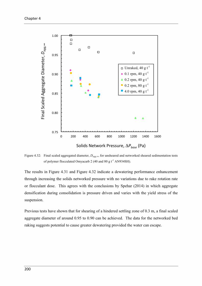
Chapter4

200

Figure 4.32: Final scaled aggregated diameter, Dagg,∞, for unsheared and networked sheared sedimentation tests

of polymer flocculated Omyacarb 2 (40 and 80 g t-1 AN934SH).

The results in Figure 4.31 and Figure 4.32 indicate a dewatering performance enhancement

through increasing the solids networked pressure with no variations due to rake rotation rate

or flocculant dose. This agrees with the conclusions by Spehar (2014) in which aggregate

densification during consolidation is pressure driven and varies with the yield stress of the

suspension.

Previous tests have shown that for shearing of a hindered settling zone of 0.3 m, a final scaled

aggregate diameter of around 0.95 to 0.90 can be achieved. The data for the networked bed

raking suggests potential to cause greater dewatering provided the water can escape.

0.75

0.80

0.85

0.90

0.95

1.00

0 200 400 600 800 1000 1200 1400 1600

FinalScaledAg

gregateDiam

eter,D

agg,∞

SolidsNetworkPressure,ΔPbase(Pa)

Unraked,40gt

0.1rpm,40gt

0.2rpm,40g/t

0.2rpm,80gt

4rpm,40gt

Unraked, 40 g t-1

0.1 rpm, 40 g t-1

0.2 rpm, 40 g t-1

0.2 rpm, 80 g t-1

4.0 rpm, 40 g t-1

RakedBatchSettling

201

4.8 Overall Discussion and Conclusions

A series of sheared and un-sheared batch settling tests have been performed using calcite

(Omyacarb 2) at various conditions. The rate and extent of aggregate densification as a

function of experimental conditions were determined. Results have shown enhancements in

aggregate densification can be achieved depending on operational conditions.

It was predicted that the rate of aggregate densification is independent of initial height and a

strong function of shear rate. The extent of aggregate densification is proportional to the

raking duration multiplied by the rate of aggregate densification. Given sufficient raking

time, the final scaled aggregate diameter, a measure of extent of densification, was shown to

be independent of rake rotation rate. The extent of aggregate densification however increased

with network pressure indicating rake pressure on the aggregates is the driving force for

densification.

So far results have looked at the effect of experimental variables while raking either during

the entire settling test or within a single dewatering regime, sedimentation, or consolidation.

Comparison between these sets of experiments is discussed below with the aim of providing

insight into rake location within a thickener for optimal dewatering due to shear.

4.8.1 Raking zones

To recognise the optimal rake location within a thickener, this chapter considered the effects

of raking a suspension during either sedimentation or consolidation in isolation. Raked batch

settling tests with raking during both dewatering regimes were also performed. Figure 4.33

and Figure 4.34 presents the resultant aggregate densification parameters for all settling tests

performed within this experimental program as a function of rake rotation rate. Results from

batch settling tests by van Deventer (2012) have also been included. The zone in which

raking was performed for each batch settling test has been highlighted.

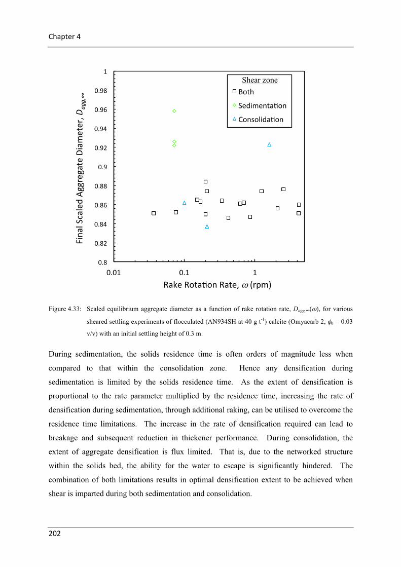
Chapter4

202

Figure 4.33: Scaled equilibrium aggregate diameter as a function of rake rotation rate, Dagg,∞(ω), for various

sheared settling experiments of flocculated (AN934SH at 40 g t-1) calcite (Omyacarb 2, φ0 = 0.03

v/v) with an initial settling height of 0.3 m.

During sedimentation, the solids residence time is often orders of magnitude less when

compared to that within the consolidation zone. Hence any densification during

sedimentation is limited by the solids residence time. As the extent of densification is

proportional to the rate parameter multiplied by the residence time, increasing the rate of

densification during sedimentation, through additional raking, can be utilised to overcome the

residence time limitations. The increase in the rate of densification required can lead to

breakage and subsequent reduction in thickener performance. During consolidation, the

extent of aggregate densification is flux limited. That is, due to the networked structure

within the solids bed, the ability for the water to escape is significantly hindered. The

combination of both limitations results in optimal densification extent to be achieved when

shear is imparted during both sedimentation and consolidation.

0.8

0.82

0.84

0.86

0.88

0.9

0.92

0.94

0.96

0.98

1

0.01 0.1 1

FinalScaledAg

gregateDiam

eter,D

agg,∞


Both

Sedimentanon

Consolidanon

Shear zone

RakedBatchSettling

203

Figure 4.34: Rate of densification, A, (s-1), as a function of rake rotation rate for flocculated (AN934SH at

40 g t-1) calcite (Omyacarb 2, φ0 = 0.03 v/v) with an initial settling height of 0.3 m. The zone in

which shear was imparted is highlight. Additional result by van Deventer (2012) is also included.

Again, due to residence time limitations during sedimentation and flux limitations during

consolidation, results indicate an optimal rate of aggregate densification is obtained when

raking during both sedimentation and consolidation. Further sheared batch settling tests of

raking during sedimentation at higher rake rotation rates is recommended in order to confirm

this conclusion.

0.00001

0.0001

0.001

0.01

0.01 0.1 1

RateParam

eterfo

rAggregateDen

sificano

n,

A(s

-1)


Both

Sedimentanon

Consolidanon

Chapter4

204

205

Chapter 5. FULL SCALE PREDICTION FROM

LAB SCALE CHARACTERISATION

Chapter 5

Full Scale Prediction from Lab Scale

Characterisation

Chapter 3 presented both thickener performance and solids concentration profile predictions

for a model material representative of a flocculated industrial slurry. Chapter 4 provided

material characterisation and aggregate densification parameter trends through a series of

experiments using a representative industrial slurry, calcite (Omyacarb 2). This chapter

utilises the experimental results and model to predict thickener performance based on a real

material. This demonstrates the ability to predict full scale thickener performance from

laboratory scale batch settling tests and characterisation techniques.

Typically within industry, dynamic thickening in the way of small scale thickeners with rakes

and continuous feed, overflow and underflow is employed to perform the majority of

practical thickener sizing and test work. The advantage of dynamic testing is that a

relationship between the solids flux, underflow concentration, and overflow clarity can be

determined. However, as it is a dynamic test, there are also disadvantages including the large

amount of material required, time required to achieve steady state and issues regarding

achieving constant flocculation conditions. Also present is the subjective nature of scale up

and related full scale thickener performance predictions.

The proposed method within this thesis of predicting thickener performance through from a

series of batch settling tests and theoretical modelling overcomes the issues related to

dynamic testing such as those mentioned above. However, this method is unable to provide

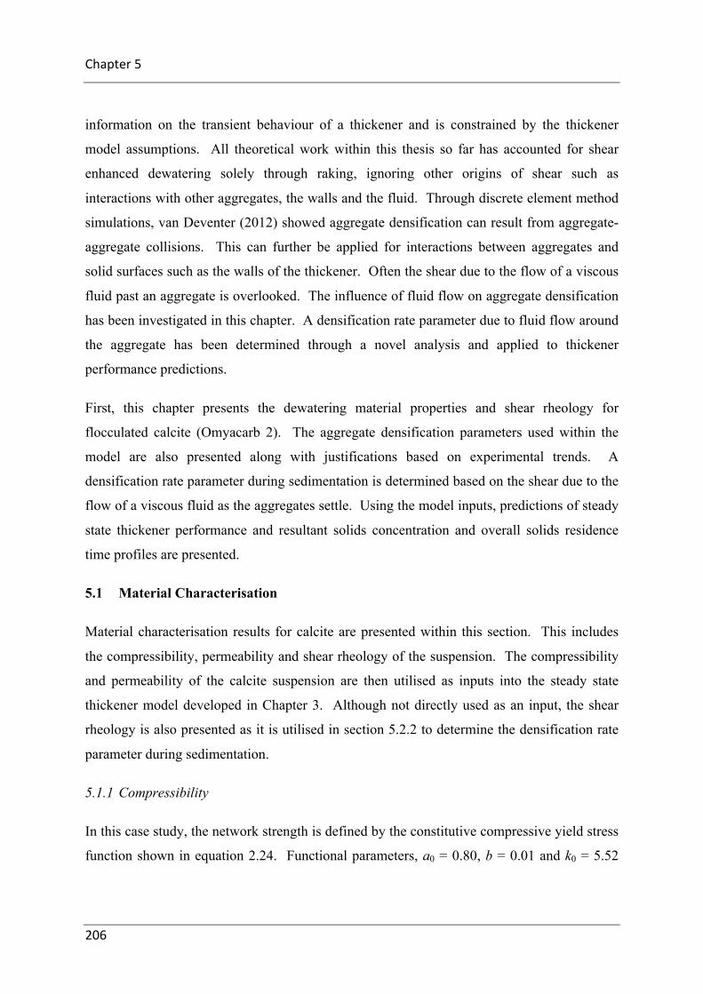
Chapter5

206

information on the transient behaviour of a thickener and is constrained by the thickener

model assumptions. All theoretical work within this thesis so far has accounted for shear

enhanced dewatering solely through raking, ignoring other origins of shear such as

interactions with other aggregates, the walls and the fluid. Through discrete element method

simulations, van Deventer (2012) showed aggregate densification can result from aggregate-

aggregate collisions. This can further be applied for interactions between aggregates and

solid surfaces such as the walls of the thickener. Often the shear due to the flow of a viscous

fluid past an aggregate is overlooked. The influence of fluid flow on aggregate densification

has been investigated in this chapter. A densification rate parameter due to fluid flow around

the aggregate has been determined through a novel analysis and applied to thickener

performance predictions.

First, this chapter presents the dewatering material properties and shear rheology for

flocculated calcite (Omyacarb 2). The aggregate densification parameters used within the

model are also presented along with justifications based on experimental trends. A

densification rate parameter during sedimentation is determined based on the shear due to the

flow of a viscous fluid as the aggregates settle. Using the model inputs, predictions of steady

state thickener performance and resultant solids concentration and overall solids residence

time profiles are presented.

5.1 Material Characterisation

Material characterisation results for calcite are presented within this section. This includes

the compressibility, permeability and shear rheology of the suspension. The compressibility

and permeability of the calcite suspension are then utilised as inputs into the steady state

thickener model developed in Chapter 3. Although not directly used as an input, the shear

rheology is also presented as it is utilised in section 5.2.2 to determine the densification rate

parameter during sedimentation.

5.1.1 Compressibility

In this case study, the network strength is defined by the constitutive compressive yield stress

function shown in equation 2.24. Functional parameters, a0 = 0.80, b = 0.01 and k0 = 5.52

FullScalePredictionfromLabScaleCharacterisation

207

were used to described the compressibility of flocculated calcite, as indicated by

experimental analysis (see section 4.5.4). The close packing volume fraction is the maximum

possible solids concentration achievable, set to φcp = 0.63 v/v. The initial gel point and

aggregate packing volume fraction are φg,0 = 0.188 and ϕp = 0.6 respectively. The resultant

compressive yield stress function is depicted in Figure 5.1.

5.1.2 Permeability

The steady state thickener model developed in Chapter 3 requires the hindered settling

function in terms of a constitutive equation as an input. In this case study, the permeability is

defined by the constitutive hindered settling function shown in equation 2.34. The hindered

settling function dictated by experimental analysis resulting from the settling of flocculated

(40 g t-1 AN934SH) calcite (Omyacarb 2, φ0 = 0.03 v/v) (see section 4.5.4) is fitted to

equation 2.34. Resultant fitting parameters values; ra, rg, rn and rb are; 6.37 x 1012, -0.028,

4.14 and 0, respectively. Experimental hindered settling data and the curve fit are presented

in Figure 5.1.

Additionally, the liquid is assumed to be water, with a viscosity of η = 0.001 Pa s and density

ρliq = 1000 kg m-3. The density of Omyacarb 2 is ρsol = 2710 kg m-3 as given by MatWeb

(2014).

Chapter5

208

Figure 5.1: Un-densified compressive yield stress and hindered settling functions, Py,0(φ) & R0(φ), used within

the model case study. Py,0(φ) and R0(φ) were determined via fitting equations 2.24 and 2.34 to

experimental data resulting in fitting parameter values of ra = 6.37 x 1012, rg = -0.028, rn = 4.14, a0

= 0.80, b = 0.01, k0 = 5.52, φg,= 0.188 v/v and φcp, = 0.63 v/v.

5.1.3 Shear rheology

Spehar (2014) presented the rheological parameters for flocculated calcite at a range of solids

volume fractions, φ, through both cup and bob and vane techniques (Nguyen and Boger

1985). For modelling purposes, the Herschel-Bulkley model was used to describe the shear

stress, τ, vs. shear rate, γ! , behaviour. The resultant fitting parameters, K and n, as functions

of solids concentration, φ, are depicted in Figure 5.2. Ensuring K and n approach the values

for water as solids concentration approaches zero (K(φ=0) = 0.001 Pa s and n(φ=0) = 1),

Herschel–Bulkley fitting parameters as functions of solids concentration were obtained from

curve fits of the data. K(φ) and n(φ) are given by,

⎭⎬⎫

⎩⎨⎧

≥

≤=

v/v034.0:v/v034.0:

0695.0001.0

)( 7243.9

39.134

φ

φφ

φ

φ

ee

K (5.1)

and

1.E-02

1.E-01

1.E+00

1.E+01

1.E+02

0 0.1 0.2 0.3 0.4 0.5

Compressiv

eYieldStress,P

y(φ)(KP

a)

SolidsVolumeFracnon,φ(v/v)

Series1CurveFitData

1.E+06

1.E+07

1.E+08

1.E+09

1.E+10

1.E+11

1.E+12

0 0.1 0.2 0.3 0.4

Hind

ered

Sep

lingFuncno

n,

R(φ)(Kgs-

1 m-3)


Curve Fit Data


209

⎭⎬⎫

⎩⎨⎧

≥

≤=

−

v/v03.0:v/v03.0:

3724.0

)(925.32

φ

φφ

φen . (5.2)

Figure 5.2: Herschel-Bulkley paramters, K(φ) and n(φ) used to describe the shear rheology of flocculated

Omyacarb 2. Data from Spehar (2014)

The shear stress, τ, and suspension viscosity, η, for a given solids concentration, φ, as a

function of shear rate, γ! , is given by the Herschel-Bulkley model equations, equations 2.21

and 2.22. For a range of solids concentrations, φ, the functional form of the shear stress, τ

and viscosity, η, as a function of shear rate, γ! , is shown in Figure 5.3. A scalar ratio, α =

Py/τy, of order 20 can be expected for mineral flocculated suspensions.

1.E-03

1.E-02

1.E-01

1.E+00

1.E+01

1.E+02

0 0.1 0.2 0.3 0.4 0.5Herschel-BulkleyFiu

ngParam

eter,

K(φ)(Pasn)


K

KCurveFitData

0.E+00

2.E-01

4.E-01

6.E-01

8.E-01

1.E+00

1.E+00

0 0.1 0.2 0.3 0.4 0.5Herschel-BulkleyFiu

ngParam

eter,

n(φ)


nnCurveFitData

Chapter5

210

Figure 5.3: Shear stress, τ, and viscosity, η, as a function of shear rate, γ for flocculated calcite (Omyacarb 2)

at various solids concentrations, φ, given by equations 2.21 and 2.22. Shear rheology has been

modelled using a Herschel-Bulkley fit with parameter’s, K(φ) and n(φ) described by equation 5.1

and 5.2. A nominal value of 20 has been used for the ratio between the compressive and shear

yield stresses, α, for solids concentrations of 0.2 and 0.3 v/v.

5.2 Aggregate Densification Parameters

The aggregate densification parameters used to predict full-scale thickening of a flocculated

calcite suspension are presented within this section. Aggregate densification parameters

include the equilibrium scaled aggregate diameter, Dagg,∞, and the densification rate

parameter during sedimentation, As, and consolidation, Abed.

5.2.1 Extent of aggregate densification

An equilibrium scaled aggregate diameter, Dagg,∞, of 0.86 was used to describe the maximum

extent of aggregate densification. This value is representative of the results obtained from the

analysis of sheared settling tests of flocculated (40 g t-1 AN934SH) calcite (Omyacarb 2, φ0 =

0.03 v/v), (see section 4.5.5).

5.2.2 Shear during sedimentation

In Chapter 4, the densification rate parameter for shear during sedimentation due to raking

was determined to be of order 7 x 10-5 s-1. Shear on a settling aggregate may also arise from

0.00001

0.0001

0.001

0.01

0.1

1

10

100

0.1 1 10 100 1000

ShearS

tress,τ(P

a)

ShearRate(s-1)

00.030.120.20.3

1.E-04

1.E-03

1.E-02

1.E-01

1.E+00

1.E+01

1.E+02

1.E+03

1.E+04

1.E+05

0.1 1 10 100 1000

Viscosity

,η(P

a.s)

ShearRate(s-1)

00.030.120.20.3

φ

φ


211

the flow of the viscous process liquor past the surface of the aggregate. This section explores

the impact of shear during sedimentation by deriving from first principles the shear stress on

an isolated settling particle in creeping flow. The implications of the inherent assumptions

within this derivation are discussed along with methods to account for these assumptions

upon application to settling aggregates. Furthermore, the shear stress on an aggregate due to

settling is converted to an effective densification rate parameter using experimental results.

This rate parameter, As, is then incorporated into thickener modelling as in input in section

5.4.

5.2.2.1 Theory: Shear stress on a settling sphere

During sedimentation, within the dilute zone in a thickener, the solids concentration is

sufficiently small such that aggregates effectively settle as isolated spheres in the process

liquor. The shear rate imparted on an aggregate due to settling can be determined by

considering the creeping flow of an incompressible fluid around a fixed solid sphere of radius

rp and diameter dp. The definition and implications of creeping flow are discussed later. The

velocity distribution for creeping flow around a sphere can be determined via Navier-Stokes

equations in spherical coordinates (r, θ, Φ). The velocity distribution is given by,

θcos21

23

13

⎥⎥⎦

⎤

⎢⎢⎣

⎡⎟⎟⎠

⎞⎜⎜⎝

⎛+⎟⎟⎠

⎞⎜⎜⎝

⎛−= ∞ r

rrr

uu ppr , (5.3)

θθ sin41

231

3

⎥⎥⎦

⎤

⎢⎢⎣

⎡⎟⎟⎠

⎞⎜⎜⎝

⎛+⎟⎟⎠

⎞⎜⎜⎝

⎛+−= ∞ r

rrr

uu pp , (5.4)

and

0=Φu , (5.5)

where ur, uθ, uΦ are the velocities in the r, θ and Φ directions (Bird et al. 2006) and θ is

measured such that θ = 0° at the front of the particle and θ = 180° at the rear. The pressure

due to fluid motion, p, is given by

Chapter5

212

θη

cos23

2

⎟⎟⎠

⎞⎜⎜⎝

⎛−= ∞

rr

rup p

p

, (5.6)

while the pressure at the surface of the sphere, p0, is given by,

θη

cos3

0p

rr dupp

p

∞= −== . (5.7)

The components of the stress tensor τ are obtained by substituting the velocity distributions,

equations 5.3, 5.4 and 5.5, into the stress tensor according to Newton’s law of viscosity. The

stress distribution is given by,

θη

τττ θθ cos3

2242

⎥⎥⎦

⎤

⎢⎢⎣

⎡⎟⎟⎠

⎞⎜⎜⎝

⎛+⎟⎟

⎠

⎞⎜⎜⎝

⎛−=−=−= ∞

ΦΦ rr

rr

ru pp

prr (5.8)

and

θη

ττ θθ sin23

4

⎟⎟⎠

⎞⎜⎜⎝

⎛== ∞

rr

ru p

prr , (5.9)

where all other components are zero. Equation 5.8 describes the normal stresses while

equation 5.9 gives the shear stress. The shear stress at the surface of the sphere, τ0, due to

fluid motion is therefore given as,

θη

ττ sin30

prr d

up

∞= == . (5.10)

Accounting for the non-isolated nature of the settling particle, the shear stress at the surface

of the particle as a function of solids concentration, φ, is given by rearrangement and

substitution of the modified Stokes law, equation 2.32, resulting in

( )θ

φφρη

θφη

θφτ sin),(

13sin),(3),,(2

0pp

pp

p DRg

dDu

dD −Δ

== . (5.11)


213

The maximum shear stress on the particle surface, when θ = 90°, is

),(3

),(max,0 pp

p Dud

D φη

φτ = . (5.12)

The average shear stress across the entire sphere surface is given by,

),(23

)(

)()(),(

0

0,0 p

pp

p

pave Dud

dA

dAD φ

η

θθ

θθφτ

φτ π

π

==

∫

∫, (5.13)

where Ap(θ) is the surface area of the aggregate at θ given by

θπθ sin)( pp dA = . (5.14)

Thus, equation 5.13 can be used to determine the average shear stress on the surface of an

aggregate within a thickener due to sedimentation. Derivation of equation 5.13 assumes

creeping flow around the particle and that the settling particle is both spherical and behaves

as a rigid body with no flow occurring within the particle. These assumptions must be

considered when applying equation 5.13 to determine the shear stress within the dilute zone

of a thickener.

5.2.2.2 Shear stress on an aggregate

A flocculated aggregate is neither solid, spherical nor a rigid body. Application of equation

5.13 on a settling aggregate must consider the implications of the inherent assumptions

during derivation. Within this section, drag coefficient correction factors are presented as a

method to account for the assumptions of creeping flow and a non-slip boundary condition.

The assumption of a solid spherical particle is also discussed.

Providing the assumptions are reasonable or have been corrected, along with an

understanding of the relationship between shear rate and rate of aggregate densification

through experimental results, equation 5.13 can be used to determine an effective

Chapter5

214

densification rate parameter due to settling alone. Application of equation 5.13 to an

aggregate is such that the particle radius, diameter and scaled diameter is given by the

aggregate radius, diameter and scaled diameter, rp = ragg, dp = dagg, and Dp = Dagg.

Creeping flow

Creeping flow is defined such that the particle Reynolds number, Rep, is less than about 0.1

with an absence of eddy formation downstream from the aggregate. The particle Reynolds

number is given by equation 2.5 where u∞ is the free stream velocity which when applied to a

settling aggregate, is given by the aggregate settling velocity, u(φ, Dagg). The aggregate

diameter can be expressed in terms of the original undensified aggregate diameter, dagg,0, and

the extent of densification such that Dagg = dagg/dagg,0. Substituting for the scaled diameter

and the aggregate settling velocity results in a particle Reynolds number as a function of

solids concentration, φ, and densification extent, given by,

( )),(

1),(),(Re2

0,0,

aggagg

aggliqagg

agg

aggliqaggp DRD

dDu

Dd

Dφ

φρη

ρφ

η

ρφ

−Δ== , (5.15)

where Dagg is the scaled particle diameter due to densification and Δρ is the density

difference (ρsol-ρliq). For a given densification extent and solids concentration, equation 5.15

can be used to calculate the particle Reynolds number to be used in subsequent calculations

to determine the drag coefficient.

Depending on the particle Reynolds number, the drag coefficient is given by either CD,Stokes,

CD,int, or CD,Newton (equations 2.7, 2.8 and 2.9). Thus, a drag force correction factor, χint and

χNewton, can be defined to account for deviations from the Stokes drag coefficient as the

particle Reynolds number increases (creeping flow no longer applies). The correction factor,

χint, and χNewton is therefore given by,

7.0

,

int,int Re14.01 p

stokesD

D

CC

−==χ , (5.16)

and


215

54Re

,

, p

stokesD

NewtonDNewton C

C≈=χ . (5.17)

As the drag coefficient is inversely proportional to the settling velocity, assuming creeping

flow at Rep > 0.1 will result in an error in the settling velocity equivalent to the drag

coefficient error. At Rep = 1, Stokes law predicts a drag force that is about 10% too low

(Bird et al. 2006). The drag coefficient correction factor as a function of particle Reynolds

number due to the flow regime, χRep, is shown in Figure 5.4 and given by,

3

37.0Re

10Re10Re1.01.0Re

for 54Re

Re14.011

)(Re>

≤<

≤

⎪⎩

⎪⎨

⎧

+=

p

p

p

p

pppχ . (5.18)

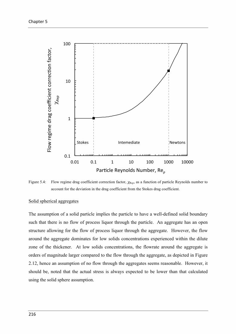
Chapter5

216

Figure 5.4: Flow regime drag coefficient correction factor, χRep, as a function of particle Reynolds number to

account for the deviation in the drag coefficient from the Stokes drag coefficient.

Solid spherical aggregates

The assumption of a solid particle implies the particle to have a well-defined solid boundary

such that there is no flow of process liquor through the particle. An aggregate has an open

structure allowing for the flow of process liquor through the aggregate. However, the flow

around the aggregate dominates for low solids concentrations experienced within the dilute

zone of the thickener. At low solids concentrations, the flowrate around the aggregate is

orders of magnitude larger compared to the flow through the aggregate, as depicted in Figure

2.12, hence an assumption of no flow through the aggregates seems reasonable. However, it

should be, noted that the actual stress is always expected to be lower than that calculated

using the solid sphere assumption.

0.1

1

10

100

0.01 0.1 1 10 100 1000 10000

Flow

regimedragcoe

fficien

tcorrecnon

factor,

χ Rep

ParncleReynoldsNumber,Rep

StokesIntemediateNewtons


217

Slip boundary condition

Derivation of equation 5.13 also assumed aggregates as rigid bodies and hence applied a non-

slip boundary condition at the surface of the sphere. An aggregate has no clearly defined

solid boundary resulting in a perfect slip condition at the surface. A perfect slip condition

results in a decreased velocity gradient at the surface of the sphere and a subsequent

reduction in the shear stress. For application to settling aggregates, a drag coefficient

correction factor due to the slip boundary condition, χBC, can be applied, where χBC is given

by,

slipnonD

slipDBC C

C

−

=,

,χ . (5.19)

Datta and Deo (2002) presented the drag coefficient as a function of solids concentration for

rigid body spheres (no slip) and bubbles (perfect slip). The reduction in drag coefficients for

rigid bodies and bubbles is presented in Figure 5.5.

Chapter5

218

Figure 5.5: Ratio of perfect slip to no slip drag coefficients, χBC = CD,slip/CD,non-slip, as a function of solids

volume fraction, φ. Ratios calculated based on drag coefficient values determined by Datta and

Deo (2002).

Utilising a perfect slip boundary, the resultant drag coefficient is approximately 40 to 60 %

less than that obtained using a no slip boundary condition. These values agree with

observations by Faltas and Saad (2011) and Kishore and Ramteke (2016). A drag coefficient

factor, χBC, of 0.5 has been applied to calculations of the shear stress and aggregate diameter

in order to account for the presence of a non-slip boundary.

Overall drag coefficient

Accounting for non-creep flow and a slip boundary condition, the overall drag coefficient of

an aggregate is given by,

0

0.1

0.2

0.3

0.4

0.5

0.6

0.7

0.8

0.9

1

0 0.02 0.04 0.06 0.08 0.1

Slipdragcoeffi

cien

tcorrecnon

factor,χ

BC

SolidsConcentreanon,φ(v/v)


219

BCStokesDpaggD pCC χχRe,, )(Re = , (5.20)

where χBC and χRep are drag coefficient correction factors and CD,Stokes is the Stokes drag

coefficient, 24/Rep. Equation 5.20 can subsequently be implemented in shear stress

calculations in order to apply equation 5.13 and calculate the shear stress on a settling

aggregate.

5.2.2.3 Experimental trends

As noted earlier, a Herschel-Bulkley model can be applied to describe the relationship

between the shear stress and shear rate. CFD simulations resulted in a linear relationship

between shear rate and rake rotation rate, equation 4.1. The relationship between shear stress

and rake rotation rate for a given solids concentration is given by combining the two, such

that,

( )ny K ωττ 6.0+= . (5.21)

The relationship between the densification rate parameter, A (s-1), and rake rotation rate, ω

(rpm), for flocculated (40 g t-1 AN934SH) calcite (Omyacarb 2, φ0 = 0.03 v/v) was

determined through a series of raked settling tests (see section 4.5.5). The result is depicted

in Figure 5.6 and given by equation 4.4, reiterated below:

⎭⎬⎫

⎩⎨⎧

>

≤

×

×=

−

−

16.016.0

1068.17

1086.7)( 4

4

ω

ωωωA . (4.4)

The solids concentration, φ, ranged from the initial solids concentration, φ0 = 0.03, up to the

fan limit, φfl = 0.118, in the sheared batch settling tests and subsequent analysis used to

determine equation 4.4. Application of equation 5.21 at φ = φ0 and φ = φfl, provides the

minimum and maximum shear stress as a function of rake rotation rate experienced within the

sheared settling tests, depicted in Figure 5.6. At these concentrations the Herschel-Bulkley

fitting parameters were determined to be K(φ0) = 0.056, K(φfl) = 0.22, n(φ0) = n(φfl) = 0.3724

via equations 5.1 and 5.2. The average solids concentration during the settling tests can be

Chapter5

220

approximated as the average between the initial and fan limit concentration, φave = (φ0+φfl)/2 =

0.074 v/v. The resultant shear stress from the average solids concentration is also depicted in

Figure 5.6. Utilising τ(ω) and Α(ω), the densification rate parameter can be expressed as a

direct function of shear stress, as depicted in Figure 5.7.

Figure 5.6: (a) Shear stress, τ, as a function of rake rotation rate determined via equation 5.21 at solids

concentration, φ = φ0 = 0.03, φ = φfl = 0.118 and φ = φave = 0.074 v/v.

(b) Densification rate parameter, A (s-1), as a function of rake rotation rate, ω, given by equation

4.4 and determined from sheared batch settling tests of flocculated (40 g t-1 AN934SH) calcite

(Omyacarb 2, φ0 = 0.03 v/v)

00.10.20.30.40.50.60.70.80.91

0.0001 0.01 1 100

ShearS

tress,τ(P

a)


0.030.0740.118

1.E-08

1.E-07

1.E-06

1.E-05

1.E-04

1.E-03

1.E-02

1.E-01

1.E+00

0.00010.001 0.01 0.1 1 10 100

Densificano

nRa

teParam

eter,A


φ0 φave φfl


221

Figure 5.7: Densification rate parameter, A (s-1), as a function of shear stress, τ, based on CFD simulations

and experimentally observed trends (equations 5.21 and 4.4)

For an average shear stress on the surface of a settling aggregate in a viscous fluid, an

effective densification rate parameter due to sedimentation, As, can be determined via the

results depicted in Figure 5.7.

5.2.2.4 Application: Flocculated calcite

This section utilises the above theory, experimental trends and correction factors to determine

a densification rate parameter due to the settling of flocculated calcite within the

sedimentation zone of a thickener. This includes the calculation of; the undensified (Dagg =

Dagg,0 = 1) and fully densified (Dagg = Dagg,∞ = 0.86) aggregate properties, particle Reynolds

number, average shear stress on a settling particle, equivalent rake rotation rate and finally

the densification rate parameter due to sedimentation.

1.E-07

1.E-06

1.E-05

1.E-04

1.E-03

1.E-02

0.001 0.01 0.1 1

Densificano

nRa

teParam

eter,A

(s-1)

ShearStress,τ(Pa)

0.03

0.074

0.118

φ0

φave

φfl

Chapter5

222

For gel points, φg,0 = 0.188 v/v and φg,∞ = 0.30 v/v, and aggregate packing fraction, ϕp = 0.6,

the solids concentrations within the aggregate, φagg,0 and φagg,∞, were determined to be 0.32

and 0.50 v/v, via equation 2.62. The densities of undensified and fully densified aggregates,

ρagg,0 and ρagg,∞, are given by equation 2.59 and were calculated to be 1541 and 1851 kg m-3

respectively.

The hindered settling function of an isolated aggregate, using the R(φ, Dagg) parameter values

in section 5.1, is calculated to be, R(0, 1) = 2.37 x 106 kg s-1 m-3 and R(0, Dagg,∞) = 2.04 x 10-6

kg s-1 m-3. For a solid particle settling in water, ρliq = 1000 kg m-3 and η = 0.001 Pa s, and g

= 9.8 m s-2, the undensified and fully densified isolated aggregate settling velocities are

calculated to be u(0, 1) = 0.0071 m s-1 and u(0, Dagg,∞) = 0.0082 m s-1, via equation 2.71.

Assuming the liquid flow through the aggregate is negligible relative to the flow around the

aggregate, the initial aggregate diameter can be inferred through a force balance, equation

2.1. Substituting in terms for the gravitational, buoyancy and drag force, results in the

settling velocity as a function of the drag coefficient, equation 2.10. The drag coefficient for

an aggregate, given by equation 5.20, is a function of particle Reynolds number and

subsequently dependent on the aggregate diameter. Through iterative methods, an isolated

calcite aggregate, φ ≈ 0, has an inferred initial aggregate diameter, dagg,0 = 116 µm with a

particle Reynolds number of Rep = 0.82. A fully densified isolated aggregate subsequently

has an aggregate diameter of dagg,∞ = 100 µm and a particle Reynolds number, Rep = 0.82.

The aggregate drag coefficient of an isolated aggregate was calculated to be CD,agg(φ = 0) =

16.4.

The settling velocity, u(φ, Dagg), and particle Reynolds number, Rep(φ, Dagg), for calcite was

calculated via the modified Stokes equation, 2.73, and the particle Reynolds number

equation, 5.15. The resultant values are depicted in Figure 5.8.


223

Figure 5.8: Particle settling velocity, u, and Reynolds number, Rep, vs. solids concentration, φ, for an

undensified (Dagg = 1) and fully densified (Dagg = Dagg,∞ = 0.86) calcite aggregate, ρsol = 2710 kg

m-3 and dagg,0 = 116 µm, settling in water, ρliq = 1000 kg m-3 and η = 0.001 Pa s.

At high solids concentrations, φ > φagg, aggregate structure becomes independent of formation

conditions. As a result, the particle Reynolds number at these high concentrations is given by

the undensified particle Reynolds number, Rep(φ, Dagg = 1).

From the particle Reynolds numbers, the assumption of creeping flow is reasonable for solids

concentrations greater than 0.018 v/v for un-densified aggregates, Dagg = 1, and 0.028 v/v for

fully densified aggregates, Dagg = Dagg,∞= 0.86. Accounting for non-creeping flow and a

full-slip boundary condition, the shear stress on the surface of a settling aggregate, τ0,agg, is

given by equation 5.13 multiplied by the drag coefficient correction factors, χRep and χBC

such that,

BCsphereagg pχχττ Re,0,0 = , (5.22)

where τ0,sphere is the average shear stress on the surface of a settling sphere given by equation

5.13. As stated above, χBC = 0.5 while χRep is given by equations and 5.18. The average and

maximum shear stress, τ0,ave and τ0,max, experienced by the aggregate at a range of solids

1.E-08

1.E-07

1.E-06

1.E-05

1.E-04

1.E-03

1.E-02

0 0.1 0.2 0.3 0.4 0.5

SeplingVe

locity,u(m

s-1 )


Dagg=1uinf

1.E-06

1.E-05

1.E-04

1.E-03

1.E-02

1.E-01

1.E+00

0 0.1 0.2 0.3 0.4 0.5

ParncleRe

ynoldsNum

ber,Re

p


Re0Reinf

Dagg = 1

Dagg = Dagg,∞ = 0.86 Dagg, = 1


Chapter5

224

concentrations has been calculated for the settling of flocculated calcite via equations 5.12,

5.13 and 5.22 and is depicted in Figure 5.9.

Figure 5.9: (a) Aggregate drag coefficient, CD,agg, as a function of solids volume fraction for the

sedimentation of flocculated calcite (Omyacarb 2, 40 g t-1 AN934SH). The drag coefficient has

been corrected to account for flow regime and full slip boundary condition.

(b) Average and maximum shear stress, τ0, on the surface of an undensified (Dagg = 1) and fully

densified (Dagg = Dagg,∞ = 0.86) calcite aggregate, dagg,0 = 116 µm and ρsol = 2710 kg m-3, due to

the flow of water, ρliq = 1000 kg m-3 and η = 0.001 Pa s, around the aggregate. Shear stress has

been adjusted to account for flow regime and slip boundary condition.

From equations 5.21 and 5.22, the relationship between the shear stress on a settling

aggregate and an experimental rake rotation rate can be defined. Utilising equation 4.4

provides the densification rate parameter as a function of the shear stress on the surface of the

aggregate. The settling densification rate parameter as a function of solids concentration,

As(φ), for flocculated calcite is depicted in Figure 5.10.

Experimentally, a maximum densification rate parameter of 1.77 x 10-3 s-1 was obtained

corresponding to a critical rake rotation rate of 0.16 rpm. For the majority of solids

concentrations, the settling rate alone produces a densification rate less than that obtained

through raking. This result is significant in that it illustrates that settling alone is insufficient

1.E+00

1.E+01

1.E+02

1.E+03

1.E+04

1.E+05

1.E+06

1.E+07

1.E+08

0 0.1 0.2 0.3 0.4 0.5

AggreegateDragCo

efficien

t,CD,agg


0

inf

1.E-08

1.E-07

1.E-06

1.E-05

1.E-04

1.E-03

1.E-02

1.E-01

1.E+00

0 0.1 0.2 0.3 0.4 0.5ShearS

tress,τ0,agg


0inf0inf

τ0,max(φ, Dagg = 1)

τ0,max(φ, Dagg,∞)

τ0,ave(φ, Dagg = 1)

τ0,ave(φ, Dagg,∞)

Dagg = 1 Dagg = Dagg,∞ = 0.86


225

to maximise the aggregate densification rate. Additional shear through raking is suggested to

further increase the rate of densification during sedimentation.

Figure 5.10: Densification rate parameter, As (s-1), as a function of solids volume fraction, φ, due to the flow of

the process liquor around an undensified (Dagg = 1) and fully densified (Dagg = Dagg,∞ = 0.86)

flocculated calcite (Omyacab 2) aggregate. As determined at φ0 = 0.03 and φfl = 0.118 are also

shown (dashed lines) to indicated the maximum (φ0) and minimum (φfl) possible values.

The one-dimensional steady state thickener model algorithm presented in Chapter 3 utilises a

constant densification rate parameter above the suspension bed, As. As seen in Figure 5.10,

As is a strong function of solids concentration and densification extent, which in the current

form of the model algorithm, cannot be implemented.

The solids residence time of an aggregate within the sedimentation zone of a thickener is

related to the settling rate. Increasing the settling rate reduces the solids residence time.

However, the densification rate due to sedimentation is at a maximum at low solids

1.E-12

1.E-11

1.E-10

1.E-09

1.E-08

1.E-07

1.E-06

1.E-05

1.E-04

1.E-03

1.E-02

0 0.02 0.04 0.06 0.08 0.1 0.12

Densificano

nRa

teParam

eter,A

s(s-1)


0

inf

phi0

phi0

phifl

phifl

As(φ, Dagg = 1)

As (φ, Dagg = 0.86)

As,max(φ, Dagg = 1)

As,max((φ, Dagg = 0.86)

As,min(φ, Dagg = 1)

As,min(φ, Dagg = 0.86)

Chapter5

226

concentration, corresponding to high settling rates. This results in high densification rates

with low residence time at high fluxes and low densification rates with high residence times

at low fluxes. This trade-off between solids residence time and densification rate renders any

densification during sedimentation to be of insignificant impact to the overall thickener

performance. This was demonstrated in Chapter 3, where thickener predictions using a

model material were performed with a densification rate during sedimentation of 10-4 s-1.

This value corresponds to the maximum observed due to sedimentation shown in Figure 5.10

above.

To demonstrate the maximum potential increase in thickener throughput, although expected

to be insignificant, a value of 10-4 s-1 will be implemented in thickener predictions using the

material properties of calcite.

5.2.3 Shear during consolidation

The rate of aggregate densification achieved in a sheared batch settling test within the lab is

expected to be greater than the rate of densification achieved during the practical operation of

a thickener. Within close proximity of the rakes, the rate of densification observed should

represent a value similar to that obtained experimentally, however the majority of the bed is

only exposed to the shear and compressive stresses from the rakes for a portion of the time.

This periodic exposure occurs within laboratory raking, but is more significant in full scale

thickener operation. For the rest of the time, the aggregates are not exposed to significant

shear. The overall result is that the expected rate of densification in a thickener is a fraction

of that observed experimentally. A good indicator of the fraction would be to quantify the

proportion of time that an aggregate is exposed to shear stresses greater than a critical

threshold where aggregate densification is significant. This fraction can be quantified

through CFD modelling and can vary with geometry and rake speed. In general, a laboratory

raking rig is expected to apply shear more consistently than a full scale thickener. Therefore,

a laboratory raking rig might expose particles to the critical shear rate only 10% of the time,

but this exposure might only occur 1% of the time in a full scale thickener. As a result, for a

laboratory measured densification rate parameter of A = 10-3 s-1, the effective value in full

scale operation might be as low as Aeffective = 10-4 s-1.


227

An average densification rate parameter value of order 10-3 s-1 was observed experimentally.

However, in order to model full scale thickener performance, a densification rate parameter

within the suspension bed, Abed, of 10-4 s-1 has been used for the modelling of flocculated

calcite thickening.

5.3 Summarised Thickener Model Inputs

5.3.1 Operational conditions

A thickener feed height of 5 m, a bed height of 2 m and a feed solids concentration of 0.03

v/v will be used, representing typical values seen within industry. Some models such as

(Usher and Scales 2005) include a factor to account for change in thickener cross sectional

area but for the purposes of the model here, the thickener will be assumed to be straight

walled with no cross sectional area variation.

5.3.2 Material properties

All modelling results presented within this chapter utilise the material properties, including

Py(φ) and R(φ) curve fits and densification parameters, applicable to the prediction of

flocculated calcite thickening as presented above. A summary of the model inputs is

presented in Table 5-1.

Table 5-1: Summary of steady state thickener model inputs for the prediction of thickener performance using

flocculate calcite as the suspension.

Py(φ) & R(φ) ρsol

(kg m-3) ρliq

(kg m-3) Dagg,∞

(-) As

(s-1) Abed

(s-1) hb

(m) hf

(m) φ0

(v/v) Curve fits as presented in

Section 5.1 1000 2710 0.86 10-4 10-4 2 5 0.03

5.4 Results: Solids Flux vs. Underflow Solids Concentration

Predictions of steady state solids flux vs. underflow solids concentrations are shown in Figure

5.11 for operation of a straight walled thickener (no cross sectional area variation). These

predictions are based on suspension characterisation through small scale batch settling

experiments and subsequent analysis. This prediction shows significant improvement in both

the solids flux and underflow solids concentration due to aggregate densification. The

Chapter5

228

improvement due to densification within the sedimentation zone can be quantified via a

performance enhancement factor given by equation 3.6, and depicted in Figure 5.12.


underflow solids volume fraction for rates of aggregate densification Abed = 10-4 s-1 and As = 0 and

10-4 s-1. Aggregate densification and thickener operation parameters of Dagg,∞ = 0.86, hf = 5 m,

hb = 2 m and φ0 = 0.03 v/v were used. Upper and lower solids flux predictions (Dagg = 1 and

Dagg = Dagg,∞) are also shown. Open symbols represent permeability limited (PL) solutions while

filled symbols represent compressibility limited (CL) solutions. Solid lines indicate the maximum

or minimum potential solutions.

0.0001

0.001

0.01

0.1

1

10

0 0.1 0.2 0.3 0.4 0.5

SolidsF

lux,q(ton

nesh

r-1m

-2)


0

As = 0, CL

As = 10-4 s-1, CL

As = 0, PL

As = 10-4 s-1, PL

Dagg = 1


Feed flux limit


229

Figure 5.12: Performance enhancement factor, PE, as a function of underflow solids concentrations due to the

incorporation of As = 10-4 s-1.

Comparing the performance enhancement obtained for As = 0 and 10-4 s-1 indicates that

densification due to sedimentation on the overall solids flux is minimal. If densification is to

be exploited during sedimentation, where rake torque and flux limitations are minimised,

additional shear through raking is required. Prior to φu = 0.12 v/v, steady state solids flux for

the modelled system is feed flux limited and hence raking during sedimentation results in no

performance enhancement (PE = 1). At φu = 0.12 v/v, the solution becomes permeability

limited and therefore raking during sedimentation results in a performance enhancement.

This performance enhancement diminishes as φu becomes greater as raking during

compression becomes more prevalent. At underflow concentrations above 0.25 v/v, the

solids residence time and rate of densification within the networked bed is sufficient such that

complete densification occurs resulting in no performance enhancement (PE = 1).

1

1.01

1.02

1.03

1.04

1.05

0 0.1 0.2 0.3 0.4 0.5

PerformanceEnh

acem

ent,PE


Chapter5

230

Steady state (straight walled) thickener predictions for a bed height of 1 m have been

performed. The predicted solids flux vs. underflow solids concentration for both bed heights,

1 m and 2 m, is depicted in Figure 5.13. The solids flux at a bed height of 1 m is observed to

approach the solids flux for a bed height of 2 m while sedimentation limited, however upon

compression diverges.


underflow solids volume fraction for rates of aggregate densification Abed = 10-4 s-1 and

As = 10-4 s-1. Aggregate densification and thickener operation parameters of Dagg,∞ = 0.86, hb = 1

and 2 m and φ0 = 0.03 v/v were used. Upper and lower solids flux predictions (Dagg = 1 and

Dagg = Dagg,∞) are also shown. Open symbols represent permeability limited (PL) solutions while

filled symbols represent compressibility limited (CL) solutions. Solid lines indicate the maximum

or minimum potential solutions.

0.0001

0.001

0.01

0.1

1

10

0 0.1 0.2 0.3 0.4 0.5

SolidsF

lux,q(ton

nesh

r-1m

-2)


qk

q

qk

q

hb = 2 m, PL

hb = 2m, CL

hb = 1m, PL

hb = 1m, CL

Dagg = 1

Dagg = Dagg,∞

q(φ0)


231

5.5 Conclusion

Flocculated calcite has been characterised through lab scale sheared and unsheared settling

tests. Characterisation results have been presented and subsequently used as inputs into the

one-dimensional steady state thickener model incorporating dynamic densification outlined in

Chapter 3. The procedure for full scale thickener prediction from lab scale characterisation

has been demonstrated through utilising experimentally determined material properties for

flocculated calcite as inputs into the developed 1D SST model.

Methods have been developed to quantify the rate of aggregate densification due to the flow

of a viscous fluid past a settling aggregate. Experimental results have shown a densification

rate parameter of 10-3 s-1 can be achieved within laboratory sheared settling tests when raking

at shear rates above 0.1 s-1. Due to the uneven distribution of shear within a thickener, this

can potentially correspond to a lower effective densification rate of 10-4 s-1 within a thickener.

Due to the flow of fluid around an aggregate, a densification rate parameter of 10-4 s-1 can be

achieved for a highly diluted suspension, similar to values obtained through raking.

However, densification due to sedimentation rapidly decreases with solids concentration due

to the decrease in settling velocity. Application of a densification rate parameter during

sedimentation was performed, with results showing a minimal impact on thickener

performance. The extent of densification is proportional to both solids residence time and the

rate of aggregate densification. This minimal impact of densification during sedimentation is

a result of the very low solids residence time and a densification rate which diminishes as the

solids concentration increases. Note however, that even though the addition of mechanical

shear through raking within the sedimentation zone has the potential to increase the rate of

densification, the impact will be limited by the low solids residence time.

Chapter5

232

233

Chapter 6. MODEL APPLICATIONS

Chapter 6

Model Applications

This chapter utilises the experimental observations in Chapter 4 and the one-dimensional

steady state thickener (1D SST) model developed in Chapter 3 to further explore practical

applications. Discussion topics include;

• Changes in suspension dewatering material properties

• Shear during sedimentation

• Shear during compression

• Underflow limitations

• Process optimisation

6.1 Changes in Material Properties

Changes in material properties occur due to flocculation, feed mixing, aggregate

densification, polymer behaviour, and aggregate breakage. A change in the dewatering

properties of a material via all of these mechanisms can occur within a thickener and will

affect the overall performance. The model developed in Chapter 3 accounts for flocculation

and aggregate densification, while the effects of feed mixing, polymer behaviour and

aggregate breakage are not taken into account. The various methods by which the material

properties of a suspension can vary and effect overall thickener performance are discussed

below.

Chapter6

234

6.1.1 Flocculation

Flocculation is most commonly performed within the feed well, pipe or launder system of a

thickener. Flocculation involves the aggregation of fine particles into aggregates to increase

the sedimentation rate. The increase in sedimentation rate comes at a cost, as the gel point

decreases with flocculant dose, decreasing the extent of compression in the networked

suspension bed.

The model developed in Chapter 3 accounts for flocculation by using the material properties,

R(φ) and Py(φ), of the flocculated suspension as inputs. For the polyacrylamide flocculant

used within this thesis, maximum activity is achieved between 48 and 72 after which minimal

change in polymer activity occurs (Owen et al. 2002). Flocculant used within this thesis for

experiments have a time frame up to 140 h (including material preparation time) while

modelling results in Chapter 3 indicate a maximum solids residence time of 3 h. As a result

any changes in the properties of the flocculant over time, such as polymer degradation, are

not taken into account.

In determining the optimum flocculant dose, the following must be considered; the shear

yield stress of the suspension, flocculation efficiency and the ability to effectively shear and

densify the aggregates.

The shear yield stress of the suspension gives rise to limitations on the maximum rake speed

through operational limitations on the rake torque. In order to pump the underflow stream,

the shear yield stress also provides an upper limit on underflow solids concentration. The

shear yield stress increases with increasing flocculant dose. Therefore, as flocculant dose

increases, the maximum rake speed and underflow solids concentration decreases.

The type and dose of flocculant greatly influences the resultant aggregate size, shape, and

response to shear. An increase in aggregate strength, and size results from increasing the

number of bonds formed through an increase in flocculant dose. As a consequence, overall

settling velocity increases. This increase in strength results in an aggregate that is less

responsive to shear induced densification. On the other hand, reduction in flocculant dose

results in floc structures that are weak. This allows for either fast and efficient densification

ModelApplications

235

or complete aggregate breakage in the presence of shear. An unflocculated particle has a

significantly reduced settling velocity. As solid particles are relatively incompressible, shear

has virtually no impact on the structure or density in a thickener.

At high flocculant doses, large, fast settling aggregates can form quickly, but they may also

settle before all of the fine particles are aggregated. The consequence is poor flocculation

resulting in an aggregate size distribution and subsequent size segregation within the

thickener. The thickener model used herein assumes line settling and with this, no variation

in particle/aggregate size. Further research and development is required to incorporate

particle size distributions into the model.

Using the material properties, R(φ) and Py(φ), for various flocculant dosages and the 1D SST

model in Chapter 3, predictions of thickener performance offer a simple method for

determining the optimal flocculant dose. These predictions also describe the change in

underflow shear yield stress with flocculant dose given knowledge of the shear rheology of

the suspension. This provides the ability to optimise flocculant dosage based on raking and

pumping limitations. Full characterisation of the densification parameters through lab scale

settling tests is required to investigate the response to shear due to flocculant dose.

6.1.2 Feed densification state

The size, shape, and strength of an aggregate leaving the feedwell of a thickener are generally

dependent on the flocculation regime within the feedwell. Upon exiting the feedwell,

according to the model assumption of line settling, all material moves directly away from the

feed height without mixing and therefore aggregates enter the thickener in an un-densified

state, Dagg = 1 at z = hf. However, in real systems there are aggregate density distributions,

flow of particles in all directions and mixing effectively causing aggregates at the feed height

to have an average aggregate diameter less than that produced during flocculation within the

feedwell.

Although the thickener model does not account for mixing at a given feed height, this can be

modelled by altering the initial densification state, Dagg,0, to a value less than 1. A reasonable

knowledge on the amount of aggregate densification caused by feed mixing is required. The

Chapter6

236

operation of a recycle loop or shear within the feedwell during flocculation may also result in

an effective initial scaled aggregate diameter less than 1. This is difficult given the need for

dilution but may happen naturally in some systems.

As an example, steady state (straight walled) thickener model predictions using the material

properties and operational conditions presented in Chapter 3 were predicted for a feed

densification state of Dagg,0 = 1, 0.95 and 0.80 as depicted in Figure 3.28. Utilising these

predictions, response curves can be generated indicating the effect of Dagg,0 on the underflow

solids concentration when operating at constant solids flux, as depicted in Figure 6.1. As

expected, an increase in the underflow solids concentration is obtained through decreasing

the feed aggregate diameter at a given operating flux. Less densification is required within

the thickener. This effect is most significant at solids fluxes between 0.5 and 2 tonnes hr-1

m-2. It should be noted that Figure 6.1 provides the steady state solution when the aggregate

diameter of the feed is altered. It does not provide any indication of the time scale required to

reach these steady states.

Alternatively, the effect of Dagg,0 on the solids flux while operating at constant underflow

concentration can also be generated and is depicted in Figure 6.2. Here reduction in the feed

aggregate diameter results in increased solids flux for a given operating underflow

concentration.

ModelApplications

237

Figure 6.1: Effect of feed aggregate diameter, Dagg,0, on underflow solids concentration, φu (v/v), for operation

at various solids flux, q (tonnes hr-1 m-2). Results based on thickener predictions using a model

material with hf = 5 m, hb = 2m, φ0 = 0.05 v/v, Dagg,∞ = 0.80, As = 0 and Abed = 10-4 s-1. Any points

within the shaded region are at a reduced bed height (hb < 2m).

0

0.05

0.1

0.15

0.2

0.25

0.3

0.35

0.4

0.45

0.5

0.8 0.85 0.9 0.95 1

Und

erflo

wSolidsC

oncentrano

n,φ

u(v/v)

FeedScaledAggregateDiameter,Dagg,0

0.01 0.20.5 12 10

q (tonnes hr-1 m-2)

Chapter6

238

Figure 6.2: Effect of feed aggregate diameter, Dagg,0, on solids flux, q (tonnes hr-1 m-2) for operation at

various underflow solids concentrations, φu (v/v). Results based on thickener predictions using a

model material with hf = 5 m, hb = 2m, φ0 = 0.05 v/v, Dagg,∞ = 0.80, As = 0 and Abed = 10-4 s-1. Any

points above the dashed line are at a reduced bed height (hb < 2).

6.1.3 Stimuli responsive polymers

Changes in the solubility and adsorptions properties of a flocculant are known to change the

dewatering properties of a suspension within the thickener. Stimuli responsive flocculants

have been the topic of numerous research programs (Li et al. 2007, Franks et al. 2014, Yang

et al. 2015). Polymer stimuli include time, temperature, pH, light, and solvent conditions.

Within thickening, it is desirable to have a high sedimentation rate within the dilute zone and

high extent of compression within the suspension bed. One method to achieve this is to have

a stimuli responsive polymer that de-activates with a stimulus such as reduced temperature.

1.E-02

1.E-01

1.E+00

1.E+01

0.8 0.85 0.9 0.95 1

SolidsF

lux,q(ton

nesh

r-1m

-2)

FeedScaledAggregateDiameter,Dagg,0

0.060.10.150.20.250.3

φu (v/v)

ModelApplications

239

Therefore temperature control of the suspension bed would than allow for the polymer to

deactivate, potentially increasing the overall thickener performance.

The thickener model does not account for changes in dewatering material properties due to

the change in flocculant-particle interactions. However, with slight modifications to the

algorithm, stimuli responsive polymers can be partially accounted for through incorporation

of a switch in R(φ) and Py(φ) parameter values at a given residence time or height.

Development of material properties that are not only functions of aggregate densification, but

also the properties of the polymer requires further work.

6.1.4 Aggregate densification

Aggregate structure changes through shear are accounted for via aggregate densification

whereby the aggregate size is reduced and intra-aggregate liquid is expelled. The tortuosities

around the aggregates decrease resulting in an overall increase in suspension permeability

and as a consequence, an increase in the settling rate of the suspension. This decrease in

aggregate diameter also increases the gel point of the suspension, lowering the overall

compressibility. The magnitude of the changes in the material properties is dependent on the

magnitude and time scale of shear applied to the aggregates. The changes in material

properties due to aggregate densification have been discussed in detail in section 2.7.

Parameters, A and Dagg,∞, are used as model inputs for time dependent material properties,

Py(φ,t) and R(φ,t), in order to account for shear effects through aggregate densification.

Currently, constant aggregate densification parameters are used as model inputs and are

determined based on experimental results and analysis as outlined in sections 2.7.5 and 3.3.

Previous research (van Deventer et al. 2011, Spehar 2014), along with the associated

experimental results observed (see section 4.5.4 and 6.3.1), indicates that constant aggregate

densification parameters are inadequate to fully capture the rate and extent of aggregate

densification. Observations suggest aggregate parameters are sensitive to solids

concentration, bed depth, and pressure, with an optimum rate of densification occurring

above a critical shear rate. For improved SST predictions, incorporation of aggregate

densification functionality is recommended, however not preformed within this work.

Chapter6

240

6.1.5 Aggregate breakage

At high shear rates, there arises the potential for aggregates to break and create either smaller

aggregates or erode small aggregates and isolated particles, effectively reducing the

sedimentation rate and increasing the compressibility. The model assumes all shear effects

are accounted for through aggregate densification and hence the influence of aggregate

breakage is neglected. Breakage leads to smaller aggregates which settle a little slower

overall. Incorporation of the combination of smaller aggregates and primary particles

requires the removal of the line settling assumption and hence further work involving the

further development of the theory to account for particle size distributions is required.

6.2 Shear during Sedimentation

Traditionally raking within a thickener is used to transport material to the underflow, with

raking and subsequent direct shearing of aggregates only performed within the suspension

bed at the base of the thickener. Hence, the majority of steady state thickener performance

predictions so far, have assumed all shear and aggregate densification occurs within the

suspension bed and all aggregates are un-densified, Dagg = 1, at the top of the bed, z = hb.

In reality, this is not the case as shear during sedimentation can occur due to the flow of the

process liquor past the surface of a settling aggregate (see section 5.2.2) as well as from

aggregate-aggregate and aggregate-wall interactions plus rake disturbances. Providing

mechanical shear through raking within the dilute zone of the thickener will also cause shear

and subsequent aggregate densification during sedimentation.

The solids residence time during sedimentation is often orders of magnitude less when

compared to the consolidation zone (see section 3.8.7). The extent of densification is

proportional to the rate of densification and the shear exposure time. Hence, dewatering

enhancement due to shear during sedimentation is limited by the low solids residence time.

6.2.1 Mechanical shear during sedimentation

The rate of aggregate densification achieved from settling aggregates alone is non-trivial,

however it can be further increased through the addition of mechanical shear, such as raking,

ModelApplications

241

within the dilute zone of the thickener. Previous research has investigated raking during

sedimentation with results indicating a significant improvement in overall thickener

performance (Loan and Arbuthnot 2010).

During sedimentation, the settling rate is not hindered by a suspension network which would

resist consolidation. By definition, the compressive and shear yield stress during

sedimentation is zero, resulting in a significantly reduced rake torque. However, scaling and

solids build-up on the rake can be problematic over long operating campaigns.

6.3 Shear during Compression

Traditionally, raking is used as a means to transport material to the underflow in order to

supply sediment to the discharge pump to prevent both caking (locally high solids

concentrations) and channel formation. However recent observations, including results

presented within this thesis, indicate that raking causes shear induced dewatering (Novak and

Bandak 1994, Johnson et al. 1996, Channell and Zukoski 1997, Gladman et al. 2005, Usher et

al. 2009, Gladman et al. 2010, Usher et al. 2010, van Deventer et al. 2011, Grassia et al.

2014, Spehar et al. 2015). As raking is predominately implemented within the networked

suspension bed, logically, discussions regarding the implications of shear during compression

within a thickener are required. Discussion topics on shear during compression presented

below include; solids concentration effects, flux limitations, bed height effects and rake

torque limitations.

It should be noted that aggregate densification describes the phenomenon of shear induced

reduction in aggregate diameter in which intra-aggregate liquor is expelled. Within the

networked bed, an interconnected network is formed in which an aggregate is less defined.

Aggregate densification theory can be applied to quantify the extent and rate of shear induced

dewatering enhancement, however it is the tearing, and rearrangement of the networked

structure due to shear that can enable enhanced dewatering. Note however, that over-

shearing has been shown to produce a relatively homogenous mixture with poor permeability

(Usher 2002)

Chapter6

242

6.3.1 Solids concentration effect on densification parameters

It has been demonstrated (see Chapter 2, Chapter 4 and van Deventer et al. (2011)) that

aggregate densification parameters can be inferred from simple sheared batch settling tests

using a modified Kynch method. This method assumes constant rate and extent parameters,

without consideration of the solids concentration and the subsequent effect on densification.

Figure 4.15 (replotted below) depicts the sediment interface height for the sheared settling of

flocculated calcite. The predicted sediment interface height determined using the modified

Kynch analysis method is also depicted. A predicted increase in the settling velocity at low

solids concentrations and decreased settling velocity at high solids concentrations results

from the application of a constant densification rate parameter, A. This trend was observed

for the majority of sheared batch settling tests conducted throughout this work as well as in

the experimental results presented by van Deventer (2012). This implies a constant

densification rate parameter is insufficient and the possibility of a local solids concentration,

φ(t) dependence (as well as shear rate, ω, see section 4.5.5). Other possible dependences

include non-uniform changes in aggregate density and aggregate dimensions as densification

occurs.

ModelApplications

243

Figure 4-15: Predicted sediment interface height, h(t), curve fit incorporating aggregate densification using the

optimum value of A (0.00135 s-1). Predicted and experimental data represents batch settling tests

of flocculated (AN934SH at 40 g t-1) calcite (Omyacarb 2, φ0 = 0.03 v/v) with an initial height of

0.263 m.

At larger times, the majority of aggregates are present within a networked suspension bed at

the base of the settling cylinder. By definition, the networked suspension bed is at solids

concentrations greater than or equal to the solids gel point, φg. At these concentrations the

suspension exhibits a compressive and shear yield stress. Due to the shear yield stress, an

uneven distribution of shear is imparted onto the suspension, such that significant shear is

experienced near the rake pickets with comparatively less shear between the rake pickets.

Furthermore, Spehar (2014) concluded that densification is driven by the pressure imparted

by the rakes, which in turn is a strong function of shear yield stress. This implies that an

increased rate of densification is achieved at larger times due to the presence of the shear

yield stress.

0

0.05

0.1

0.15

0.2

0.25

0.3

0 500 1000 1500 2000

Hei

ght,

h (m

)

Time, t (s)

Sheared Sedimentation

Predicted Settling

Chapter6

244

At early time, the majority of aggregates are within the hindered settling regime and at solids

concentrations less than the gel point, resulting is a shear yield stress of zero. This zero shear

yield stress significantly reduces the pressure in front of the rakes, resulting in an expected

reduction in the rate of densification compared to larger times, when a shear yield stress is

present. The reduced solids concentrations also result in a reduced number of aggregate

interactions resulting in densification. This implies that the rate of densification increases as

concentration increases.

Methods utilised in Chapter 4 optimise the curve fit across the sedimentation portion of the

settling curve to obtain an average densification rate parameter. Application of curve fitting

over different time scales or settling regimes provides a simple method to account for the

solids concentration dependence in the densification rate. It is recommended to determine the

densification rate through application of curve fitting over the fan region, obtaining a value

for the rate parameter for the fan region as well as a value for both the start and end of the

fan, pre-fan and late fan respectively. Using the fitting method for the start and the end of the

fan region allows for a split function where A has a different value, such that:

⎪⎩

⎪⎨

⎧

=

≤<

=

= )(

fl

flprefan

prefan

latefan

fan

prefan

AAA

Aφφ

φφφ

φφ

φ , (6.1)

where φprefan and φfl are the solids concentrations at the start and end of the fan region.

Utilisation of a split function provides a reduced curve fit error through empirical methods.

Optimisation of the densification rate parameter to the pre-fan, fan and late fan settling zones

provides results as shown in Figure 6.3.

Data for Figure 6.3 was produced via 18 raked settling tests of flocculated (40 g t-1

AN934SH) calcite suspension (Omyacarb 2, φ0 = 0.03 v/v) with each test raked at a different

rotation rate (see section 4.5.5). Figure 6.3 illustrates that the densification rate parameter

can change significantly depending on the settling zone. For a given rake rotation rate, no

clear trend in the progression of the densification rate parameter can be observed. For

example, a rotation rate of 4.2 rpm indicates a decrease in the rate of densification over time,

whereas a rotation rate of 1.24 rpm produces no clear change in the rate. It is unclear whether

ModelApplications

245

these results are due to experimental error, poor analysis method or an actual trend that needs

investigating. This lack of clarity indicates further work into improving the current analysis

method and investigating the experimental error needs to be performed before any statements

can be made about the evolution of the rate of aggregate densification over time in a settling

test or within a thickener. The scatter presented in Figure 6.3 indicates that other phenomena,

which have not been accounted for, could be present such as aggregate breakage, or that the

relationship between the rate of aggregate densification and shear rate is weaker than other

influences such as local solids concentration.

Figure 6.3: Rate of densification, A, (s-1), as a function of shear rate for a flocculated calcite suspension (φ0 =

3 vol%) flocculated at 40 g t-1 (AN934SH). The values for A were extracted modified Kynch

method, involving curve fitting to various settling regions.

van Deventer et al. (2011) proposed a solids concentration dependence in the densification

rate parameter such that,

0.00001

0.0001

0.001

0.01

0.1

1

0.01 0.1 1 10

RateParam

eterfo

rDen

sificano

n,A(s

-1)


FiungZone

PreFan

Fan

LateFan

Chapter6

246

2)( φφ CA = , (6.2)

where C is a curve fitting parameter. Analysis using this functional form showed increased

accuracy and robustness can be achieved in sedimentation, but was not investigated in

consolidation. Within this thesis, a concentration dependent densification rate parameter was

not implemented for the analysis of sheared batch settling tests as results were used to

indicate trends and relative magnitudes as opposed to absolute values. Also, the application

of equation 6.2 resulted in an increased computational time in an already computationally

demanding process.

The developed steady state thickener model in Chapter 3 incorporates dynamic densification

through the use of a constant densification rate parameter with the option for different values

within the sedimentation and consolidation zones. The densification rate parameter is highly

dependent on the solids concentration and hence, any subsequent thickener modeller should

be aware of the subsequent implications of utilizing a constant densification rate parameter.

6.3.2 Channelling

Within the networked bed, the solids concentration is such that the particles are in close

proximity to neighbouring particles. Any dewatering, with or without shear, requires the

water to navigate between the particles within the suspension bed to reach the top of the

networked bed. These pathways are often very tortuous as indicated by the relatively large

magnitudes of the hindered settling function.

Application of shear is believed to cause rearrangement and breakage within the networked

suspension allowing for less tortuous paths to be formed. Experimental observations have

also shown the formation of channels behind the rakes, in which water has an unobstructed

pathway (Usher and Scales 2009).

6.3.3 True effect of bed height

Steady state thickener models utilise aggregate densification parameters, A and Dagg,∞, to

describe the rate and extent of dewatering enhancement due to shear. These models

ModelApplications

247

implement these densification parameters as constants. As discussed above, a constant rate

parameter is insufficient to fully capture the dynamic nature of aggregate densification.

Furthermore, experimental results (see Chapter 4) indicate a constant parameter for the extent

of aggregate densification may also be insufficient.

Experimental results show an increase in dewatering extent can be achieved through

increased bed height. Although observed, this trend is not easy to predict quantitatively as a

range of factors such as; bed depth, local solids concentration, shear rate, shear yield stress,

shear and particle/aggregate history as well as wall adhesion may influence the resultant

extent of densification. Within the networked bed, the solids concentration and shear yield

stress vary with height and therefore the experimental values for Dagg,∞as a function of solids

network pressure, Figure 4.32, represent an average value across the entire networked bed.

Although this result cannot quantitatively predict the extent of densification due to network

pressure, it illustrates the potential to increase the extent of densification through increased

network pressure.

Within the steady state thickener model (Chapter 3) the extent of densification parameter,

Dagg,∞, is implemented as a constant, with the option of different constants for the

sedimentation and consolidation regimes. Again, significant work into the theory and

implementation of the dependencies of the extent of densification is required to fully capture

and model this phenomenon.

6.3.4 Underflow limitations: Rake torque

The torque on a thickener rake arm is dependent on operational conditions such as the rake

speed, suspension bed height and the shear yield stress of the material (Usher 2002, Rudman

et al. 2008). Rake and thickener geometry also influences the resultant rake torque.

Mechanical constraints often provide an upper limit to the allowable rake torque, often due to

the limitations in the strength of the rake arms or power of the rake motor (Green and Perry

2008).

Discussion of common operational rake control methods and the impact on aggregate

densification is presented below. Application of the steady state thickener model developed

Chapter6

248

in Chapter 3 can be utilised to provide an estimate of the rake torque. The theory along with

application to a representative mineral slurry is also presented.

6.3.4.1 Operational control of rake torque

Rake torque is often controlled by either adjusting the suspension bed height, the underflow

pumping rate or the rake speed. Although reduction in the bed height or rake speed can result

in a reduction in rake torque (Rudman et al. 2008), it can also significantly impact the

resultant extent and rate of aggregate densification with implications on the overall thickener

throughput. Additionally, variations in the flocculation regime can alter the shear yield

stress, in turn influencing the rake torque (Green and Perry 2008).

Shearing the suspension bed can result in a significant increase in thickener throughput

through aggregate densification. Hence, adjusting the suspension bed height to control the

rake torque can alter thickener performance through changes in the shear regime. A

reduction in the suspension bed height such that less of the rake is submerged within the

networked bed, reduces the area for shearing of the suspension, resulting in a reduced extent

of aggregate densification and subsequent reduction in thickener output. Alternatively, an

increase in the suspension bed height such that the whole rake is submerged, reduces

pathways for channelling, and liquor escape, again resulting in a decreased thickener output.

An increase in the bed height can sometimes increase the solids concentration in the raked

portion of the bed. This increase in solids concentration increases the shear yield stress

resulting in an increase in densification extent and a further increase in the rake torque.

Providing rake torque is of no issue, it is recommended to have the top of the bed slightly

below the top of the rake, such that the entire bed is sheared and a clear pathway is available

for channels to the top of the bed.

Through lab scale experiments (see section 4.5.5), the rate of aggregate densification has

been shown to greatly depend on the shear rate, and in turn the rake speed. Hence, a

reduction in the rake speed to control the rake torque will likely decrease the extent of

aggregate densification and the overall thickener output. Conversely, high rake speeds has

the potential for breakage, particularly at the outer radii of the thickener.

ModelApplications

249

6.3.4.2 Estimates of Rake Torque: Theory

The one-dimensional steady state thickener model presented in Chapter 3 can be utilised to

obtain estimates of the rake torque based on the resultant solids concentration profiles, φ(z).

This is achieved using empirical correlations (Rudman et al. 2008) and through CFD

modelling results (Rudman et al. 2010).

Given a knowledge of the shear yield stress of the material being dewatered, τy(φ), the shear

yield stress profile, τy(z) can be determined utilising the predicted solids concentration

profiles, φ(z). The average shear yield stress, yτ , within the raking zone is given by;

( ) ( )

( )∫

∫=

r

r

h

T

h

yT

y

dzzA

dzzzA

0

0

ττ , (6.3)

where hr is the raking zone height and AT(z) is the cross-sectional area of the thickener.

Rudman et al. (2008) observed the rake torque to be relatively independent of rake speed and

a strong linear function of the suspension yield stress. The relation between the average yield

stress, yτ , and rake torque, Tq, can thus be approximated by;

0,qyq TST += τ , (6.4)

where S is a shape factor based on the rake configuration and Tq,0 is the torque experienced at

zero shear yield stress. Both S and Tq,0 are dependent on rake configuration and thickener

geometry. S and Tq,0 can be determined via direct experimental measurement or through

CFD modelling (Rudman et al. 2008, Rudman et al. 2010). The shape factor, S, would be

expected to scale with the utilised rake height which is submerged within the networked

suspension bed and raking radius. The zero shear yield stress torque, Tq,0, would be expected

to vary slightly with solids concentration due to the apparent change in viscosity.

Application of steady state thickener model predictions with equations 6.3 and 6.4 allow for

an estimate of the rake torque within a thickener.

Chapter6

250

6.3.4.3 Estimates of Rake Torque: Example application

Predictions of steady state (straight walled) thickener performance for a representative

flocculated mineral slurry were performed and presented in Chapter 3. An example of the

predicted solids concentration profiles, φ(z), for a 2 m bed height with underflow solids

concentrations ranging from 0.2 to 0.32 v/v are depicted in Figure 6.4. For underflow solids

concentrations less than 0.2 v/v, no networked bed was present within the solids

concentration profile. Hence the rake torque, Tq, at these underflow concentrations is given

by Tq,0.

Figure 6.4: Predicted solids concentration profiles, φ(z), for a range of underflow solids concentrations,

φu = 0.2 to 0.32 v/v. Predictions were performed for a representative flocculated mineral slurry

(see Chapter 3) with hf = 5 m, hb = 2 m, As = 0 s-1, Abed = 10-4 s-1, φ0 = 0.05 v/v and Dagg,∞ = 0.80.

Sudden changes in the gradient result from the transition from sedimentation to compression

limited solution.

0

0.5

1

1.5

2

2.5

3

3.5

4

4.5

5

0 0.05 0.1 0.15 0.2 0.25 0.3 0.35

Height,z(m

)


0.20.220.240.260.280.30.32

φu

ModelApplications

251

The relationship between τy(φ) and Py(φ) has been measured experimentally for a number of

systems (Buscall et al. 1987, Meeten 1994, Channell and Zukoski 1997, Green 1997, Zhou et

al. 2001, de Kretser et al. 2003, Kristjansson 2008, Spehar 2014). Based on these results, the

ratio between the shear yield stress and compressive yield stress can be approximated as a

constant. A scalar ratio of α = Py/τy = 10, will be used to relate the compressive yield stress

and shear yield stress for the representative flocculated mineral slurry. Although not used

here, other correlations (Lester et al. 2013, Lester and Buscall 2015) have proposed α to

range from an equilibrium value at high φ and approach 1 as φ approaches φg.

The compressive yield stress as a function of height, Py(z), can be determined from the

predicted z(φ), t(φ) and the constitutive equations describing Py(φ, t). The scalar ratio

between the compressive yield stress and shear yield stress, α = 10, provides τy(z) from Py(z).

The resultant shear stress profiles, τy(z) are depicted in Figure 6.5. Assuming a constant

thickener area (straight walled, AT = const.) and the entire bed is raked, hr = hb = 2 m, the

average shear stress has been calculated via equation 6.3, for each underflow concentration

and presented in Table 6-1.

Chapter6

252

Figure 6.5: Predicted shear stress profiles, τy(z), for a range of underflow solids concentrations, φu = 0.2 to

0.32 v/v. Predictions were performed for a representative flocculated mineral slurry

(see Chapter 3) with α = 10, hf = 5 m, hb = 2 m, As = 0 s-1, Abed = 10-4 s-1, φ0 = 0.05 v/v and

Dagg,∞ = 0.80.

Rudman et al. (2008) performed pilot scale thickener experiments with tailor made yield

stress slurries to measure the rake torque as a function of shear yield stress and rake rotation

rate. The pilot thickener has a height of 2 m, a diameter of 2 m and a 14° sloped floor. The

rakes comprised of two arms (geometrically opposed) spanning the pilot thickener floor.

Each arm comprised of 5 blades (290 x 75 mm) equally spaced apart at an angle of 30° to the

arm. Each blade was positioned such that no blade overlap occurred. For this rake and

thickener geometry, S and Tq,0 were determined to be 0.695 m3 and 3.35 N m respectively

(Rudman et al. 2008).

0

0.5

1

1.5

2

2.5

3

3.5

4

4.5

5

0 200 400 600 800 1000

Height,z(m

)

ShearYieldStress,τy(Pa)

0.20.220.240.260.280.30.32

φu

ModelApplications

253

Though thickener rake systems can have complex geometries, in this analysis we make the

simplifying assumption that the shape factor varies linearly with height such that S = S0hr

where S0 = 0.695 m3. Utilising the values for S0 and Tq,0 mentioned above, the rake torque,

Tq, as a function of underflow solids concentration has been calculated, via equation 6.4,

utilising the solids concentration profiles presented in Figure 6.5. The average shear yield

stress and the resultant rake torque as functions of underflow solids concentration is

summarised in Table 6-1. The rake torque is also depicted in Figure 6.6. As expected the

rake torque is constant for underflow concentrations where no networked solids bed is

present. As the networked solids bed grows with increasing solids underflow concentration,

the rake torque increases.

A simple method often employed within industry, utilises the rheology of the underflow

solids concentration as an indication of rake torque. The shear yield stress and resultant rake

torque based on the underflow rheology for the case of undensified, Dagg = 1, and fully

densified, Dagg = Dagg,∞, = 0.80, is also summarised in Table 6-1 and depicted in Figure 6.6.

Variation in rake torque with bed height is depicted in Figure 6.7.

Chapter6

254

Table 6-1: Calculated average shear stress and rake torque

φu (v/v)

τy,ave (Pa)

Tq (N m)

τy(φu,Dagg0) (Pa)

Tq(φu,Dagg,0) (N m)

τy(φu,Dagg,∞) (Pa)

Tq(φu,Dagg,∞) (N m)

0.06 - 0.10 0 3.35 0 3.35 0 3.35 0.11 0 3.35 2.54 6.88 0 3.35 0.12 0 3.35 7.77 14.2 0 3.35 0.13 0 3.35 12.8 21.2 0 3.35 0.14 0 3.35 18.0 28.4 0 3.35 0.15 0 3.35 23.7 36.2 0 3.35 0.16 0 3.35 30.1 45.2 0 3.35 0.17 0 3.35 37.7 55.7 0 3.35 0.18 0 3.35 46.7 68.2 0 3.35 0.19 0 3.35 57.5 83.3 0 3.35 0.20 4.09 9.03 70.6 102 2.20 6.40 0.21 5.99 11.7 86.7 124 29.4 44.3 0.22 8.68 15.4 106 151 59.9 86.6 0.23 12.5 20.7 131 185 90.8 130 0.24 17.9 28.3 161 226 125 177 0.25 25.6 39.0 198 278 164 232 0.26 36.8 54.5 244 343 212 297 0.27 52.9 76.9 302 424 269 378 0.28 76.7 110 375 525 341 477 0.29 112 158 468 654 430 601 0.30 164 232 585 816 541 756 0.31 244 342 734 1024 683 952 0.32 365 510 926 1290 862 1202 0.34 922 1285 1321 1839 1230 1713

ModelApplications

255

Figure 6.6: Estimated torque, Tq, as a function of underflow solids concentrations for a representative

flocculated mineral slurry (characterised in Chapter 3) calculated via equation 6.4. A rake shape

factor, S0, and zero shear yield stress torque, Tq,0, of 0.695 m3 and 3.35 N m were used. Aggregate

densification and thickener operation parameters of: hf = 5 m, hb = 2 m, hr = 2 m, As = 0, Abed = 10-

4 s-1, Dagg,∞ = 0.80, and φ0 = 0.05 v/v. Torque estimates based on undensified and fully densified

underflow rheology also depicted.

1

10

100

1000

10000

0 0.1 0.2 0.3 0.4

Torque

,Tq(N

m)


As (s-1) Abed (s-1) Dagg

0 10-4 Varies 0 0 Dagg,0 ∞ ∞ Dagg,∞

Chapter6

256

Figure 6.7: Estimated torque, Tq, as a function of underflow solids concentrations for a representative

flocculated mineral slurry (characterised in Chapter 3) for various bed heights calculated via

equation 6.4. A rake shape factor, S0, and zero shear yield stress torque, Tq,0, of 0.695 m3 and 3.35

N m were used. Aggregate densification and thickener operation parameters of: hf = 5 m, hb = 1, 2

and 4 m, hr = 2 m, As = 0, Abed = 10-4 s-1, Dagg,∞ = 0.80, and φ0 = 0.05 v/v. Torque estimates based

on undensified and fully densified underflow rheology also depicted.

Practical operation of a thickener is limited by physical constraints such as an upper limit in

applied rake torque and an upper limit in the operational rate of the underflow pump for the

underflow rheology. A simple method for determining the rake torque has been presented

above, using the thickener model to predict the suspension concentration. It is noted however

that the shear yield stress at the underflow provides a simpler indication of the ability to rake

and pump the underflow. Many paste thickener rakes and pump are unable to operate at

shear yield stresses in excess of 200 Pa (Usher and Scales 2005).

1

10

100

1000

10000

0 0.1 0.2 0.3 0.4

Torque

,Tq(N

m)


hb = 1 m

hb = 2 m

hb = 4 m

Dagg = 1

Dagg = Dagg,∞

ModelApplications

257

The scenario investigated corresponds to an approximate underflow solids concentration of

0.305 v/v. If the simple method of determining the rake torque via the underflow rheology is

applied, a resultant maximum underflow concentration between 0.25 v/v and 0.26 v/v

(depending on densification extent) is obtained. Figure 6.6 and Figure 6.7 highlights the

reduction in rake torque due to aggregate densification.

The steady state thickener model in Chapter 3 does not require knowledge of the suspension

shear rheology or underflow pump and torque limitations. Therefore, underflow solids

concentrations resulting in a shear yield stress above torque and pump limitations are

predicted (see section 3.8). In practise these underflow solids concentration are not obtained,

based on underflow rheology limitations.

6.4 Process Optimisation

It should be noted that model predictions are subject to limitations regarding the idealised

nature and assumptions of the model, however, these assumptions almost certainly represent

an upper limit to thickener performance since observed affects such as disturbed beds and

unequal redial distribution of solids (so called ‘donut’ formation) are likely to reduce

thickener performance. The steady state thickener model, developed in Chapter 3, is subject

to errors arising from the curve fitting of the compressibility and permeability of the material,

experimental errors, and the assumption of a constant rate and extent of aggregate

densification. As a result, the model predictions cannot be applied for extremely accurate

predictions, however it can provide an improved understanding of why certain underflow

solids concentrations and solids fluxes can be achieved, the trends involved and how

performance can be improved by adjustment of process variables. Process variables that can

be examined include;

• Feed concentration

• Influence of type of flocculant and flocculation conditions

• Sensitivity to process variations such as bed height

• The impact of upstream processes where the material properties such as particle size

are altered

Chapter6

258

• Solids residence time

• Rate of aggregate densification

Due to the limitation on the operational solids flux resulting from the feed solids flux, as seen

in Chapter 3, under certain conditions, the specified bed height cannot be obtained. In order

to satisfy all other operational conditions, a bed height of less than the specified height will

be obtained. In all results below, the condition where this occurs has been highlighted in

yellow on all figures displaying results.

Again, it is important to note that in all the following equations, the solids flux, q, is defined

as the volume of solids per unit time per thickener cross sectional area, with SI units of m s-1.

However, to adhere to industry conventions, all graphs of solids flux are presented in tonnes

of solids per hour per square meter, where solids throughput in tonnes of solids per hour is

simply the solids flux multiplied by the cross-sectional area of the thickener.

6.4.1 Feed concentration

Upstream processes and their efficiency dictate the feed conditions of gravity thickeners.

This can result in fluctuations in the feed conditions. The effect of feed solids concentration

was investigated in section 3.9.2. The feed solids concentration was shown to have little

impact on thickener performance at moderate to low solids fluxes. However, at very high

solids fluxes, the underflow solids concentration achieved is feed flux, q0, limited. If

operating under feed flux limitations, the underflow solids concentration is significantly

affected by both the feed solids concentration and feed flow rate.

Trends in thickener performance due to feed solid concentration fluctuations, as seen in

section 3.9.2, can be investigated by performing steady state thickener model predictions with

various feed solids concentration. As an example, steady state (straight walled) thickener

model predictions using the material properties and operational conditions presented in

Chapter 3 were performed for a feed solids concentration of φ0 = 0.005, 0.02, 0.05 and 0.08

as depicted in Figure 3.22. Additional predictions of solids flux vs. underflow solids

concentrations at various feed solids concentrations have also been performed. Utilising

ModelApplications

259

these predictions, response curves can be generated indicating the effect of φ0 on the

underflow solids concentration when operating at constant solids flux, depicted in Figure 6.8.

The solids flux is constrained by the feed limiting solids flux, q0 = q(φ0,0), as discussed in

Chapter 3. The feed limited solids flux is given by the Coe and Clevenger (1916) thickener

material balance, equation 2.108, evaluated at the feed concentration and zero time. The feed

limiting solids flux has a maximum, which corresponds to an optimum feed solids

concentration, hence the peak in the solids flux when operating at low underflow

concentrations. At high underflow concentrations, where the solids flux is less than the feed

limited solids flux, the solids flux is independent on the feed solids concentration.

Alternatively the response curves describing the impact of feed concentration on underflow

solids concentrations at constant solids flux can also be generated. Again, these response

curves provide steady state solutions and do not provide any indication of the time scale to

reach these solutions.

Chapter6

260

Figure 6.8: Effect of feed solids concentration, φ0, on solids flux, q (tonnes hr-1 m-2), for operation at various

underflow solids concentrations, φu (v/v). Results based on thickener predictions using a model

material with hf = 5 m, hb = 2m, Dagg,∞ = 0.80, As = 0 and Abed = 10-4 s-1. Any points within the

shaded region are at a reduced bed height (hb < 2m).

6.4.2 Flocculant type and flocculation conditions

Flocculation conditions, including flocculant type, can significantly alter dewatering and

densification properties of the suspension. These alterations in material properties are

discussed in 6.1.1.

Flocculation characteristics can be determined via either CFD simulations (Kahane 1999,

Nguyen 2012) or experimental methods. Experimental methods include lab scale in-line pipe

flocculation (as used within this work) or pilot scale feedwell flocculation (Farrow and Swift

1996, Heath et al. 2006, Heath et al. 2006, Heath et al. 2006). Once flocculated, performing

unsheared and sheared batch settling tests allow for material properties as a function of the

0.01

0.1

1

10

0.0001 0.001 0.01

SolidsF

lux,q(ton

nesh

r-1m

-2)

FeedSolidsConcentranon,φ0(v/v)

0.06 0.1

0.15 0.2

0.25 0.3

φu (v/v)

ModelApplications

261

flocculation conditions to be determined. Incorporation of these material properties into the

steady state thickener model in Chapter 3 provides further knowledge on the effect of

flocculation conditions on thickener throughput.

6.4.3 Bed height

Bed height can operationally be controlled and often varied in order to manipulate the rake

torque. As discussed in section 6.3.3, Dagg,∞, a measure of the extent of aggregate

densification, is strongly related to bed height. The effect of bed height on densification

extent can be investigated through a series of sheared batch settling tests with variable initial

height (see section 4.7.6). As seen in section 3.9.1, a decrease in the bed height results in a

decrease in the predicted underflow solids concentrations for a given solids flux. This change

in the extent of densification and subsequent underflow solids concentration due to bed

height change can be investigated through a series of thickener performance predictions at

various bed heights.

The impact of bed height, assuming Dagg,∞ does not vary with bed depth, can be quantified

through steady state thickener modelling. As an example, steady state (straight walled)

thickener model predictions using the material properties and operational conditions

presented in Chapter 3 were performed for bed heights of hb = 1, 2 and 4 m as depicted in

Figure 3.20. Utilising these predictions, response curves can be generated indicating the

effect of hb on the underflow solids concentration when operating at constant solids flux. The

resultant response curves are depicted in Figure 6.9. Results show an increase in the solids

flux for an increase in the bed height for a given operating flux. This effect is most

significant at high underflow solids concentrations where a bed height of a certain value must

be present in order to achieve the desired underflow solids concentration. The developed

model in Chapter 3 assumes no solids exit via the overflow. Increasing the bed height,

although it increases the solids flux, may result in a reduction in overflow clarity, which

needs to be considered.

Alternatively, a response curve can be generated that describes the change in underflow

solids concentration, φu, with bed height for operation at constant solids flux, q.

Chapter6

262

Figure 6.9: Effect of bed height, hb (m), on solids flux, q (tonnes hr-1 m-2) for operation at various underflow

solids concentrations, φu (v/v). Results based on thickener predictions using a model material

with hf = 5 m, φ0 = 0.05 v/v, Dagg,∞ = 0.80, As = 0 and Abed = 10-4 s-1. Within the shaded region, no

solution exists for the corresponding bed height and solids flux.

6.4.4 Feed particle size

Again, as a result of thickening often being the last unit in the process, the feed conditions are

subject to upstream units and their efficiency. As a result, the thickener feed stream average

particle size can fluctuate. To understand the effect of feed particle size, characterisation of

the dewatering properties and densification parameters for various particle sizes needs to be

performed. Characterisation is performed through a series of sheared and unsheared batch

settling tests (see Chapter 4). Once characterisation of a range of feed particles sizes has

been performed, the results are used within the steady state thickener model to predict the

impact of particle size and size distributions on thickener throughput.

0.0001

0.001

0.01

0.1

1

0.1 1

SolidsF

lux,q(ton

nesh

r-1m

-2)

BedHeight,hb(m)

0.15

0.2

0.25

0.3

φu

ModelApplications

263


The overall solids residence time within a thickener is of particular importance in the alumina

industry due to the presence of unstable suspensions and pregnant liquors (Usher 2002).

Significant solids residence time can result in precipitation of alumina from solution. The

steady state thickener model in Chapter 3 predicts the overall solids residence time. Hence,

solids residence time trends can be alluded to through performing steady state thickener

predictions for a range of process conditions, material properties, and densification

parameters.

6.4.6 Rate of aggregate densification

As illustrated in Chapter 3, the rate of aggregate densification can significantly alter thickener

performance. The increase in solids flux or underflow solids concentration due to variations

in densification rate can be quantified through modelling at various values for A.

As an example, steady state (straight walled) thickener model predictions using the material

properties and operational conditions presented in Chapter 3 were performed for densification

rate parameters within the suspension bed of Abed = 10-3, 10-4 and 10-5 s-1 as depicted in

Figure 3.25. Utilising these predictions, response curves can be generated indicating the

effect of Abed on the underflow solids concentration when operating at constant solids flux.

The resultant response curve is depicted in Figure 6.10. As expected, increasing the

densification rate parameter leads to an increase in the underflow solids concentration for a

given operating flux. This effect is most significant at solids fluxes between 0.05 and 0.3

tonnes hr-1 m-2.

Chapter6

264

Figure 6.10: Effect of densification rate parameter, Abed (s-1), on underflow solids concentration, φu (v/v), for

operation at various solids flux, q (tonnes hr-1 m-2). Results based on thickener predictions using a

model material with hf = 5 m, hb = 2m, φ0 = 0.05 v/v, Dagg,∞ = 0.80 and As = 0 s-1. Any points


Alternatively, the effect of Abed on the solids flux while operating at constant underflow

concentration can also be generated and is depicted in Figure 6.11. Here, an increase in the

densification rate parameter results in increased solids flux for a given operating underflow

concentration.

0

0.05

0.1

0.15

0.2

0.25

0.3

0.35

0.4

0.45

0.5

1.00E-07 1.00E-06 1.00E-05 1.00E-04 1.00E-03 1.00E-02

Und

erflo

wSolidsC

oncentrano

n,φ

u(v/v)

DensificanonRateParameter,Abed(s-1)

0.001 0.01 0.050.1 0.2 0.30.4 1 10

q

ModelApplications

265

Figure 6.11: Effect of densification rate parameter, Abed (s-1), on solids flux, q (tonnes hr-1 m-2) for operation at

various underflow solids concentrations, φu (v/v). Results based on thickener predictions using a

model material with hf = 5 m, hb = 2m, φ0 = 0.05 v/v, Dagg,∞ = 0.80 and As = 0 s-1. Any points


0.001

0.01

0.1

1

10

1.00E-07 1.00E-06 1.00E-05 1.00E-04 1.00E-03 1.00E-02

SolidsF

lux,q(ton

nesh

r-1m

-2)

DensificanonRateParameter,Abed(s-1)

0.06

0.1

0.15

0.2

0.25

0.3

φu

Chapter6

266

267

Chapter 7. CONCLUSIONS

Chapter 7

Conclusions

The objective for the research within this thesis was to provide an increased understanding of

the effect of shear on aggregates and subsequent dewatering performance of aggregated

suspensions, with specific application to gravity thickening. Through understanding the

effect of shear, the goal was to develop experimental methods that produce material

parameters to be used as inputs into thickener models, resulting in a method of process

optimisation. Overall, this research set out to answer the following question: In what settling

zone, for how long and at what shear rate should a rake or shear device be operated to

maximise dewatering performance?

To achieve these goals and answer this question, the dewatering behaviour of flocculated

suspensions under shear was investigated through a series of experimental tests while the

impact of shear on thickener performance was quantified though thickener modelling.

Incorporating experimental results into thickener modelling established a method of

quantifying influences of process variables leading to process optimisation.

Laboratory scale batch settling tests provide a simple method of characterising the dewatering

properties of suspensions. Through the addition of shear, this simple test also provides a

means of characterising the densification behaviour of flocculated suspensions. Utilising the

Chapter7

268

simple method of batch settling, the influences of process variables on densification

behaviour has been investigated.

One-dimensional thickener models that utilise material properties to predict steady state

thickener performance have been modified to account for the rate of aggregate densification.

This is the first time dynamic densification has been correctly accounted for within a

thickener model. Methods of process optimisation through utilisation of the model have been

identified.

Combining modelling and experimental results indicate shearing during compression

maximises thickener performance providing torque does not limit rake speed substantially.

Results also suggest raking the entire networked bed at a rotation rate slightly above that

which provides an optimised aggregate densification rate. This is primarily due to the solids

residence time and densification rate during sedimentation being orders of magnitude less

than that within the compression zone. This thesis provides another piece of the puzzle in

understanding the short falls of thickener modelling and how shear enhanced dewatering can

be utilised to optimise thickener performance. It also provides a simple method of predicting

full scale thickener performance through relatively simple batch settling tests and subsequent

modelling. An outline of the major outcomes resulting from this thesis is presented below.

This is followed by suggestions for further work.

7.1 Conclusions and Major Outcomes

7.1.1 Incorporation of dynamic densification into thickener models

For the first time, the dynamic nature of aggregate densification has been correctly accounted

for within thickener modelling. Theory developed for the one-dimensional steady state

thickener model combines the theories of sedimentation, consolidation, and aggregate

densification. The model takes material properties, densification parameters, and thickener

operational conditions to predict steady state thickener performance in terms of solids flux vs.

underflow solids concentration. As a result of the solution method, the model also predicts

the solids residence time and solids concentration profiles for each solids flux/underflow

solids concentration operational point.

Conclusions

269

Highlighted by the model is the presence of various operational modes depending on the

limiting factor. Previous models only considered the limiting effect of either sedimentation

or compression. Due to the dynamic nature of densification, the solids flux may also be

limited by the feed solids flux or limited by both sedimentation and compression. Under feed

solid flux limitations, the specified operational bed height cannot be obtained. For these

scenarios, the model determines the operational point based on a maximum allowable bed

height.

7.1.2 Impact of process variables on thickener performance

Methods to quantify the impact of process variables on thickener performance have been

developed. This method involves performing a sequence of thickener predictions where the

process variable of interest is altered for each prediction. Comparison of thickener

predictions provides an initial guide to the impact of the manipulated process variable.

The impact of feed aggregate diameter, bed height, feed solids concentration and

densification rate has been demonstrated for a representative mineral slurry. Response curves

for each process variable investigated have been generated. Response curves illustrate the

impact of the process variable of interest on underflow solids concentration when operating at

a constant solids flux. The inverse, effect on solids flux for constant underflow solids

concentration can also be generated.

This novel method to quantify the impact of process variables leads to improved process

optimisation. These response curves can be applied to thickener control applications. It

should be noted however, these response curves only provide the steady state solution due to

a change in proves variables, and do not provide any indication on the time scale required to

reach the steady state solution.

7.1.3 Effect of shear rate on densification parameters

Through a series of sheared batch settling tests, the effect of shear rate on densification

parameters, Dagg,∞ and A, have been quantified.

Chapter7

270

The densification rate parameter, A, was shown to be strongly related to the shear rate. At

low shear rates, A slowly increases until it reaches a critical shear rate. Above this critical

value, variation in A becomes scattered and weekly dependent on shear rate. For flocculated

calcite, a critical shear rate of 0.1 s-1 (ω = 0.16 rpm) was observed. This critical shear rate is

believed to correspond to the minimum requirement for particles to collide such that below

this value, natural aggregate kinetics allow for them to move out the way. Above this critical

shear rate, the densification rate parameter was increased by an order of magnitude compared

to values obtained below the critical value. This highlights the importance to provide

sufficient shear in order to optimise the thickening process.

The scaled equilibrium aggregate diameter, Dagg,∞, (a measure of densification extent), was

shown to be independent on shear rate providing the aggregates were exposed to shear for a

significant period of time. The change in aggregate diameter due to densification is

proportional to both the time of shear and densification rate parameter. Therefore, any

reductions in these variables have the possibility of reducing the densification extent and

compromising the operational flux of the thickener to achieve a given underflow density.

7.1.4 Effect of network stress on densification parameters

Through a series of sheared batch settling tests, the effect of network stress on densification

extent has been quantified. The initial settling height of the batch settling test was

manipulated in order to vary the network stress; with shear occurring solely on aggregates

within a networked bed.

The equilibrium scaled aggregate diameter, Dagg,∞, was observed to decrease with increasing

network stress (increase in densification extent). Variations in shear rate and flocculant dose

provided little to no variation in the values obtained, indicating the network stress as the

dominant influence. Agreeing with previous research, this trend further suggests that the

driving force for aggregate densification during consolidation is the pressure exerted by the

rakes, which varies with the shear yield stress of the suspension.

Conclusions

271

7.1.5 Effect of shear zone

One of the goals of this thesis was to provide an indication on which zone within a thickener,

sedimentation or consolidation, provides the greatest benefit in dewatering due to shear. To

answer this, sheared batch settling tests were performed in which shear was solely within

either the sedimentation or compression zones.

The densification extent achieved within the sedimentation zone was significantly less

compared to within the compression zone; however this is due to the significantly reduced

time the aggregates were exposed to shear. Comparison of densification parameters between

these sets of experiments resulted in minimal variations. However, shear during both

sedimentation and compression showed increased dewatering. This is believed to be the

result of trade-off between benefits and limitations within each zone, where shearing in both

zones maximises the benefits. Limitations include; the solids residence time, solids

concentration, network stress and flux limitations.

7.1.6 Method for full scale prediction from lab scale tests

As a tool for thickener design and optimisation, the method of predicting full scale thickener

performance from laboratory scale techniques has been developed. The method involves

characterisation of material properties and dewatering parameters through batch settling and

pressure filtration experiments, with the results employed as inputs into a 1D steady state

thickener model. This procedure has been demonstrated within this thesis based on the

material and dewatering properties of flocculated calcite.

7.1.7 Densification due to sedimentation

Shear within a thickener is predominately due to raking at the base of the thickener; however

shear also arises from aggregate interactions with the walls of the thickener and other

aggregates, as well as from the flow of the viscous fluid past the aggregate. The shear stress

on the surface of an aggregate as a result of fluid flow has been determined based on fluid

motion equations. Through experimental observations, a densification rate parameter due to

shear from the fluid, As, was determined.

Chapter7

272

The densification rate parameter due to sedimentation is proportional to the settling rate and

inversely proportional to the aggregate diameter. Hence, As decreased with increasing solids

concentration. At low solids concentrations, where settling velocity was a maximum, the

maximum value of As = 10-4 s-1, corresponds to a value obtained experimentally at low shear

rates, below the critical value. Hence, sedimentation alone is insufficient to maximise

densification within the sedimentation zone, where addition of mechanical shear such as

rakes would provide added benefit.

7.1.8 Rake torque estimates

A novel method of estimating the rake torque has been presented. Utilising predictions of

solids concentration profiles and a knowledge of the shear rheology, shear yield stress

profiles, τy(z), can be obtained. Utilising correlations between rake torque and shear yield

stress (determined experimentally or via CFD); an estimate of rake torque was obtained. The

method of obtaining rake torque has been demonstrated for a representative mineral slurry.

At low underflow solids concentrations, where the suspension is un-networked, the rake

torque remained constant. At high underflow solids concentrations, rake torque

exponentially increased with increasing underflow concentration. The effect of bed height

showed little variation in rake torque albeit at high underflow concentrations, in the limit of

approaching the maximum achievable underflow solids concentration.

7.2 Further Work and Future Directions

As with all research, there are always the unanswered questions and the endless possibilities

of further work. Research advances any understanding that we do have while adding

questions we did not know needed answering beforehand. The result of this research has

increased the knowledge of shear enhanced dewatering and points to future directions.

Suggested further work in order to expand on this research and answer any uncertainties is

presented below.

Conclusions

273

7.2.1 Aggregate densification parameter dependencies

Current aggregate densification analysis determines the densification rate parameter and

equilibrium extent of densification as constants for a given set of experimental conditions.

Experimental results presented within this thesis suggest constant densification parameters to

be insufficient in describing shear enhanced dewatering. Results indicate the possibility of a

dependency on both the local solids concentration and network stress. Other possible

dependencies include non-uniform changes in aggregate density and aggregate dimensions as

densification occurs.

Upon further work incorporating the above dependencies into densification, the resultant

theory can be included within both experimental analysis methods and additionally

incorporated into both transient batch settling and 1D steady state thickener models.

7.2.2 Model short comings

The one-dimensional steady state thickener model incorporating dynamic densification, like

all models, has its limitations. Albeit some of these limitations are inherent in the type of

model, a few limitations can be corrected for or eliminated through future research and

development.

First, the model algorithm does not account for the change in thickener cross sectional area

with height (assumes straight walled). In practise, most thickeners have a sloped base and

hence this variation should be incorporated into the model. Previous models have accounted

for this through incorporation of a shape factor; however, this term caused significant issues

with the stability of the calculation when dynamic densification was introduced. Second, the

model currently utilises constant densification parameters as inputs. As discussed above,

experiments have indicated this to be insufficient in describing aggregate densification.

Other model short comings include the assumption of equal sized aggregates with no

polydispersity and breakage. Development of the theory through accounting for

polydispersity is required before it can be subsequently incorporated into thickener

modelling.

Chapter7

274

It is suggested that further work goes into addressing such issues as particle and aggregate

size polydispersity and aggregate breakage. Furthermore, the development of a transient

model in which shear history is included is recommended.

7.2.3 Actual thickener performance

The scope of this thesis is limited to improving thickener modelling and understanding. The

one-dimensional steady state thickener model incorporating dynamic densification was used

to predict thickener performance in terms of flux vs. underflow solids concentrations along

with the solids concentration profiles. These predictions have not been compared against

actual full scale thickener measurements. Such comparisons are highly recommended as

future work and would provide invaluable insight into model discrepancies.

7.2.4 Flocculant dose

Minimal work on the effect of flocculant dose has been conducted within this thesis. The

majority of settling tests were performed at a flocculant dose that provides optimal settling

and densification conditions. The effect of flocculant dose on both material properties and

densification parameters needs to be quantified through further work. With the

characterisation of material properties and densification parameters for various flocculant

doses, the developed steady state thickener model can be employed to provide knowledge in

process optimisation due to flocculant dose.

7.2.5 Dimensionless analysis

Further work into converting parameters such as floc properties, aggregate conditions,

material properties, applied shear etc. to dimensionless values would provide a more generic

description of the phenomenon of dewatering enhancement due to shear. Conversion to

dimensionless parameters, although would provide a generic overview, practical applications

and expected values are lost in which this thesis was aimed at providing. Hence, this further

work was outside the scope of this thesis and not performed.

Conclusions

275

7.3 Overview

The work in this thesis has increased the understanding of aggregate densification and

subsequent shear enhanced dewatering. It has quantified the extent and rate of aggregate

densification for a flocculated calcite suspension and provides a new direction in laboratory

scale settling tests and subsequent characterisation. It has provided a practical tool for the

design and operation of thickeners in the minerals and other particulate fluids processing

industries.

Chapter7

276

277

REFERENCES

Auzerais, F. M., R. Jackson and W. B. Russel (1990). "The transient settling of stable and flocculated dispersions." J. Fluid Mech 221: 613-639.

Aziz, A. A. A., R. G. de Kretser, D. R. Dixon and P. J. Scales (2000). "The characterization of slurry dewatering." Water Science and Technology 41: 9-16.

Barnes, H. A., J. F. Hutton and K. Walters (1989). An introduction to rheology. Amsterdam.

Batchelor, G. K. (1972). "Sedimentation in a dilute dispersion of spheres." Journal of Fluid Mechanics 52(2): 245-268.

Bemer, D. and S. Calle (2000). "Evolution of the efficiency and pressure drop of a filter media with loading." Aerosol Science and Technology 33(5): 427-439.

Bergstrom, L. (1992). "Sedimentation of flocculated alumina suspensions: Gamma-ray measurements and comparison with model predictions." Journal of the Chemical Society, Faraday Transactions 88(21): 3201-3211.

Berres, S., R. Burger, A. Coronel and M. Sepulveda (2005). "Numerical identification of parameters for a strongly degenerate convection-diffusion problem modelling centrifugation of flocculated suspensions." Applied Numerical Mathematics 52(4): 311-337.

BGS (2015). World mineral production 2011 - 2015. Keyworth, Nottingham, British Geological Survey.

Biggs, S., M. Habgooda, G. J. Jameson and D. Yan (2000). "Aggregate structures formed via bridging flocculation mechanism." Chemical Engineering Journal(80): 13-22.

Bird, B., W. Stewart and E. Lightfoot (2006). Transport phenomena John Wiley & Sons, Inc.

Boger, D. V. (2009). "Rheology and the resource industries." Chemical Engineering Science 64(22): 4525-4536.

Brechtel, H. and H. Eipper (1990). "Improved efficiency of sewage sludge incineration by preceding sludge drying." Water Science and Technology 22(12): 269-276.

Brinkman, H. (1949). "A calculation of the viscous force exerted by a flowing fluid on a dense swarm of particles." Applied Scientific Research 1: 27-34.

Buratto, B., S. P. Usher, D. Parris and P. J. Scales (2014). "Wall effects during settling in cylinders." Colloids and Surfaces A: Physicochemical and Engineering Aspects 449: 157-169.

References

278

Burger, R. and F. Concha (1998). "Mathematical model and numerical simulation of the settling of flocculated suspensions." International Journal of Multiphase Flow 24(6): 1005-1023.

Burger, R., F. Concha and K. H. Karlsen (2001). "Phenomenological model of filtration processes: 1. Cake formation and expression." Chemical Engineering Science 56(15): 1537-4553.

Bürger, R. and K. H. Karlsen (2001). "On some upwind difference schemes for the phenomenological sedimentation-consolidation model." J. Eng. Math. 41: 145-166.

Bürger, R., K. H. Karlsen and J. D. Towers (2005). "A Model of Continuous Sedimentation of Flocculated Suspensions in Clarifier-Thickener Units." SIAM Journal on Applied Mathematics 65(3): 882-940.

Bürger, R. and A. Narváez (2007). "Steady-state, control, and capacity calculations for flocculated suspensions in clarifier–thickeners." International Journal of Mineral Processing 84(1): 274-298.

Burger, R. and W. L. Wendland (2001). "Sedimentation and suspension flows: Historical perspective and some recent developments." Journal of Engineering Mathematics 41(2): 101-116.

Buscall, R., I. J. McGowan, P. D. A. Mills, R. F. Stewart, D. Sutton, L. R. White and G. E. Yates (1987). "The rheology of strongly-flocculated suspensions." Journal of Non-Newtonian Fluid Mechanics 24(2): 183-202.

Buscall, R. and L. R. White (1987). "The consolidation of concentrated suspensions. Part 1.-The theory of sedimentation." Journal of the Chemical Society, Faraday Transactions 1: Physical Chemistry in Condensed Phases 83(3): 873-891.

Bustos, M. C. and F. Concha (1988). "In the construction of global week solutions in the Kynch theory of sedimentation." Mathematical Methods in the Applied Sciences 10: 245-264.

Bustos, M. C., F. Concha, R. Burger and E. M. Tory (1999). Sedimentation and thickening. Dordrecht, The Netherlands, Kluwer Academic Publishers.

Carman, P. C. (1956). Flow of gases through porous media, New York, Academic Press.

Caruso, F. (2006). Colloids and Colloid Assemblies: Synthesis, Modification, Organization and Utilization of Colloid Particles, Wiley.

Casson, N. (1959). Rheology of disperse systems. Ed. C.C. Mill, Pergamon Press, Oxford.

Chang, D., T. Lee, Y. Jang, M. Kim and S. Lee (1997). "Non-colloidal sedimentation compared with Kynch theory." Powder Technology 92: 81-87.

References

279

Channell, G. M., K. T. Miller and C. F. Zukoski (2000). "Effects of Microstructure on the Compressive Yield Stress." AIChE Journal 46: 72-78.

Channell, G. M. and C. F. Zukoski (1997). "Shear and compressive rheology of aggregated alumina suspensions." AIChE Journal 43: 1700-1708.

Chellam, S. and M. R. Wiesner (1993). "Fluid mechanics and fractal aggregates." Water Research 27: 1493-1496.

Cheremisinoff, N. P. (1986). Encyclopedia of fluid mechanics. G. P. Publishing. Houston.

Cheremisinoff, N. P., Ed. (2000). Gravity separation. Chemical Engineer's Condensed Encyclopedia of Process Equipment. Housten, Gulf Publishing Company.

Coe, H. S. and G. H. Clevenger (1916). "Methods for determining the capacity of slime-settling tanks." Transactions of the American Institute of Mining Engineers 60: 356-363.

Concha, F. and O. Bascur (1977). Phenomenological model of sedimentation. XII International Mineral Processing Congress, Sao Paulo, Brazil.

Condie, D., C. J. Veal, R. Amal and I. Tsui (2001). "Improving understanding of the effect of floc properties on the vacuum filtration of fine coal." Transaction Filtration Society 1: 111 - 116.

Darcy, H. (1856). "Les fontaines publiques de la ville de Dijon. Dalmont, Paris."

Datta, S. and S. Deo (2002). "Stokes flow with slip and kuwabara boundary conditions." Proceedings Mathematical Sciences 112(3): 463-475.

Davis, K. E., W. B. Russel and W. J. Glantschnig (1991). "Settling suspensions of colloidal silica: Observations and X-ray measurements." J. Chem. Soc. Faraday Trans 87: 411-424.

de Kretser, R. G., P. J. Scales and D. V. Boger (2003). "Compressive rheology: An overview." Rheology Reviews 2003: 125-166.

de Kretser, R. G., S. P. Usher, P. J. Scales, D. V. Boger and K. A. Landman (2001). "Rapid filtration measurement of dewatering design and optimization parameters." AIChE Journal 47(8): 1758-1769.

Derjaguin, B. V. and L. Landau (1941). "Theory of the stability of strongly charged lyophobic sols and of the adhesion of strongly charged particles in solutions of electrolytes." Acta Physicochim(URSS 14): 633-662.

Dickinson, E. and S. R. Euston (1991). "Computer simulation of bridging flocculation." Journal of the Chemical Society, Faraday Transactions 87: 2193-2199.

Diehl, S. (2000). "On boundary conditions and solutions for ideal clarifier-thickener units." Chemical Engineering Journal 80: 119-133.

References

280

Engquist, B. and S. Osher (1981). "One-sided difference approximations for non-linear conservation laws." Mathematics of Computation 36: 321-351.

Everett, D. H. (1988). Chapter 3: Why are colloidal dispersions stable? II. Interparticle forces, Basic principles of colloid science. London, Royal Society of Chemistry: 30-53.

Faltas, M. S. and E. I. Saad (2011). "Stokes flow past an assemblage of slip eccentric spherical particle-in-cell models." Mathematical Methods in the Applied Sciences 34(13): 1594-1605.

Farrow, J. B., R. R. M. Johnston, K. Simic and J. D. Swift (2000). "Consolidation and aggregate densification during gravity thickening." Chemical Engineering Journal 80(1–3): 141-148.

Farrow, J. B. and J. D. Swift (1996). "A new procedure for assessing the performance of flocculants." International Journal of Mineral Processing 46(3): 263-275.

Fendler, J. H. (1996). The colloidal domain: Where physics, chemistry, biology, and technology meet. . Advanced Materials, WILEY-VCH Verlag GmbH. 8: 260-260.

Fernandes, G. W., F. F. Goulart, B. D. Ranieri, M. S. Coelho, K. Dales, N. Boesche, M. Bustamante, F. A. Carvalho, D. C. Carvalho, R. Dirzo, S. Fernandes, P. M. Galetti, V. E. G. Millan, C. Mielke, J. L. Ramirez, A. Neves, C. Rogass, S. P. Ribeiro, A. Scariot and B. Soares-Filho (2016). "Deep into the mud: ecological and socio-economic impacts of the dam breach in Mariana, Brazil." Natureza & Conservação 14(2): 35-45.

Fitch, B. (1966). "Current theory and thickener design." Industrial and Engineering Chemistry 58(10): 18-28.

Fitch, B. (1983). "Kynch theory and compression zones." AIChE Journal 29(6): 940-947.

Franks, G. V., J.-P. O'Shea and E. Forbes (2014). "Controlling thickener underflow rheology using a temperature responsive flocculant." AIChE Journal 60(8): 2940-2948.

Franks, G. V., Y. Zhou, Y. D. Yan, G. J. Jameson and S. Briggs (2004). "Effect of aggregate size on sediment bed rheological properties." Physical Chemistry Chemical Physics 6: 4490-4498.

Garrido, P., R. Burgos, F. Concha and R. Burger (2003). "Software for the design and simulation of gravity thickeners." Minerals Engineering 16: 85-92.

Gibson, R. E., G. L. England and M. J. L. Hussey (1967). "The theory of one-dimensional consolidation of saturated clays." Geotechnique 17: 261-273.

Gladman, B. R. (2006). The effect of shear on dewatering of flocculated suspensions. PhD, The University of Melbourne.

References

281

Gladman, B. R., R. G. de Kretser, M. Rudman and P. J. Scales (2005). "Effect of shear on particulate suspension dewatering." Chemical Engineering Research and Design 83(7): 933-936.

Gladman, B. R., M. Rudman and P. J. Scales (2010). "The effect of shear on gravity thickening: Pilot scale modelling." Chemical Engineering Science 65(14): 4293-4301.

Grassia, P., S. P. Usher and P. J. Scales (2011). "Closed-form solutions for batch settling height from model settling flux functions." Chemical Engineering Science 66(5): 964-972.

Grassia, P., Y. Zhang, A. D. Martin, S. P. Usher, P. J. Scales, A. H. Crust and R. Spehar (2014). "Effects of aggregate densification upon thickening of kynchian suspensions." Chemical Engineering Science 111: 56-72.

Green, D. W. and R. H. Perry (2008). Perry's Chemical Engineers' Handbook (8th Edition), McGraw-Hill.

Green, M. D. (1997). Characterisation of suspensions in settling and compression. Ph.D., The University of Melbourne.

Green, M. D. and D. V. Boger (1997). "Yielding of suspensions in compression." Ind. Eng. Chem. Res. 36: 4984-4992.

Green, M. D., K. A. Landman, R. G. de Kretser and D. V. Boger (1998). "Pressure filtration technique for complete characterisation of consolidating suspensions." Ind. Eng. Chem. Res. 37: 4152-4156.

Gregory, J. (1987). "Polymer adsorbtion and flocculation in sheared suspensions." Colloids and Surfaces 31: 231-253.

Gregory, J. (1997). "The density of particle aggregates." Water Science and Technology 36.

Gruy, F. and P. Cugniet (2004). "Experimental study of small aggregate settling." Journal of Colloid and Interface Science 272: 465-471.

Hamaker, H. C. (1937). "The London-van der Waals attraction between spherical particles." Physica 4: 1058-1072.

Healy, T. W. and L. R. White (1978). "Ionizable surface group models of aqueous interfaces." Advances in Colloid and Interface Scienve 9: 303-345.

Heath, A. R., P. A. Bahri, P. D. Fawell and J. B. Farrow (2006). "Polymer flocculation of calcite: Experimental results from turbulent pipe flow." AIChE Journal 52(4): 1284-1293.

Heath, A. R., P. A. Bahri, P. D. Fawell and J. B. Farrow (2006). "Polymer flocculation of calcite: Population balance model." AIChE Journal 52(5): 1641-1653.

References

282

Heath, A. R., P. A. Bahri, P. D. Fawell and J. B. Farrow (2006). "Polymer flocculation of calcite: Relating the aggregate size to the settling rate." AIChE Journal 52(6): 1987-1994.

Heath, A. R. and P. T. L. Koh (2003). Cobined population balance modelling of particle aggregation by polymeric flocculant. Third International Conference on CFD in the Minerals and Process Industries.

Herschel, W. H. and R. Bulkley (1926). "Konsistenzmessungen von Gummi-Benzollösungen." Kolloid-Zeitschrift 39(4): 291-300.

Howells, I., K. A. Landman, A. Panjkov, C. Sirakoff and L. R. White (1990). "Time dependent batch settling of flocculated suspensions." Appl. Math. Model 14: 77-86.

Huilgol, R. R., M. Panizza, N. Phan-Thien and R. Zheng (1995). "Application of the boundary integral method to the sedimentation of irregular shaped particles." Journal of Non-Newtonian Fluid Mechanics 57: 49-60.

Hunter, R. J. (2001). "Foundations of colloid science." Oxford, Oxford University Press.

Israelachvili, J. H. (1991). "Intermolecular and surface forces." London, Academic Press Limited.

Israelachvili, J. N. and R. M. Pashley (1983). "Molecular layering of water at surfaces and origin of repulsive hydration forces." Nature 306: 249-250.

Johnson, C. P., Z. Li and B. E. Logan (1996). "Settling velocities of fractal aggregates." Enviromental Science & Technology 30: 1911-1918.

Johnson, S. B., G. V. Franks, P. J. Scales, D. V. Boger and T. W. Healy (2000). "Surface chemistry–rheology relationships in concentrated mineral suspensions." International Journal of Mineral Processing 58(1–4): 267-304.

Johnson, S. B., P. J. Scales, D. R. Dixon and M. Pascoe (2000). "Use of a superthickener device to concentrate potable water sludge." Water Research 34(1): 288-294.

Kahane, R. B. (1999). Technical advance and cost benefit from CFD modelling. Fifth International Alumina Quality Workshop, Bunbury, Western Australia.

Karl, J. R. and S. A. Wells (1999). "Numerical model of sedimentation/thicking with inertial effects." Journal of Enviromental Engineering 125(9): 792-806.

Kishore, N. and R. R. Ramteke (2016). "Slip in flow through assemblages of spherical particles at low to moderate Reynolds numbers." Chemical Engineering & Technology 39(6): 1087-1098.

Kiviti-Manor, A. (2016). Thickener dewatering optimisation for the minerals industry. Ph.D Thesis, The University of Melbourne.

References

283

Kristjansson, M. (2008). Comparison of shear and compressive yield stress ratio for sewage sludge and inorganic particulate suspensions. Masters, Aalborg University.

Krutzer, L. L. M., A. J. G. v. Diemen and H. N. Stein (1995). "The influence of the type of flow on the orthokinetic coagulation rate." Journal of Colloid and Interface Science 171: 429-438.

Kružkov, S. N. (1970). "FIRST ORDER QUASILINEAR EQUATIONS IN SEVERAL INDEPENDENT VARIABLES." Mathematics of the USSR-Sbornik 10(2): 217.

Kynch, G. J. (1952). "A theory of sedimentation." Journal of the Chemical Society: Faraday Transactions 48: 166-176.

La Mer, V. K. and T. W. Healy (1963). "Adsorption-flocculation reactions of macromolecules at the solid-liquid interface." Rev. Pure & Applied Chem. 13: 112-132.

Landman, K. A. and L. R. White (1994). "Solid/liquid separation of flocculated suspensions." Advances in Colloid and Interface Science 51(0): 175-246.

Landman, K. A., L. R. White and R. Buscall (1988). "The continuous flow gravity thickener: Steady state behaviour." AIChE Journal 34(2): 239-252.

Landman, K. A., L. R. White and M. Eberl (1995). "Pressure filtration of flocculated suspensions." AIChE Journal 41(7): 1687-1700.

Lapple, C. E. and C. B. Shepherd (1940). "Calculation of particle trajectories." Ind. Eng. Chem. 32: 605-617.

Larson, R. G., Ed. (1998). The structure and rheology of complex fluids, Oxford University Press, USA.

Lee, S. A., A. G. Fane, R. Amal and T. D. Waite (2003). "The Effect of Floc Size and Structure on Specific Cake Resistance and Compressibility in Dead-End Microfiltration." Separation Science and Technology 38(4): 869-887.

Lester, D. R. (2002). Colloidal suspension dewatering analysis. PhD Thesis, The University of Melbourne.

Lester, D. R. and R. Buscall (2015). "Correction of wall adhesion effects in batch settling of strong colloidal gels." Journal of Non-Newtonian Fluid Mechanics 221: 18-27.

Lester, D. R., R. Buscall, A. D. Stickland and P. J. Scales (2013). "Wall adhesion and constitutive modeling of strong colloidal gels." Journal of Rheology 58(1247).

Lester, D. R., S. P. Usher and P. J. Scales (2005). "Estimation of the hindered settling function from batch-settling tests." AIChE Journal 51(4): 1158-1168.

References

284

Li, D. H. and J. Fanczarczyk (1988). "Flow through activated sludge flocs." Water Research 22: 789-792.

Li, D. H., J. J. Ganczarczyk and D. Jenkins (1986). "Physical characteristics of activated sludge flocs." Critical Reviews in Environmental Control 17: 53-87.

Li, H., J. Long, Z. Xu and J. H. Masliyah (2007). "Flocculation of kaolinite clay suspensions using a temperature-sensitive polymer." AIChE Journal 53(2): 479-488.

Li, X. Y. and B. E. Logan (2001). "Permeability of fractal aggregates." Water Research 35: 3373-3380.

Lim, J. (2011). Controlling clay behaviour in suspension: Developing a new paradigm for the minerals industry. Doctor of Philosophy, The University of Melbourne.

Loan, C. and M. Arbuthnot (2010). Transforming paste thickener technology. Proceedings of the 13th International Seminar on Paste and Thickened Tailings, PASTE 2010, Toronto, Canada, Australian Centre for Geomechanics.

Mahanty, J. and B. W. Ninham (1976). Dispersion forces: Volume 1 of colloid science, Academic Press, 1976.

MatWeb. (2014). "Omya OMYACARB 10 - AZ Calcium Carbonate." Retrieved 21/2/14, from http://www.matweb.com/search/datasheet.aspx?matguid=faf74f7ab7854909bd0b12f1d13ed832&ckck=1.

Meeten, G. H. (1994). "Shear and compressive yield in the filtration of a bentonite suspension." Colloids and Surfaces A: Physicochemical and Engineering Aspects 82(1): 77-83.

Metzner, A. B., Ed. (1956). Non-newtonian technology: Fluid mechanics, mixing and heat transfer. Advances in Chemical Engineering. New York, Academic Press.

Michaels, A. S. and J. C. Bolger (1962). "Settling rates and sediment volumes of flocculated kaolin suspensions." Industrial and Engineering Chemistry Fundamentals 1: 24-33.

Mills, P. D. A., J. W. Goodwin and B. W. Grover (1991). "Shear field modification of strongly flocculated suspensions — Aggregate morphology." Colloid & Polymer Science 269(9): 949-963.

Mueller, J. A., K. G. Voelkel and W. C. Boyle (1966). "Nominal diameter of floc related to oxygen transfer." Am. Soc. Civ. Eng. J.Sanit. Eng. Div. 92: 9-20.

Mular, A. L. and D. J. Barratt (2002). Mineral processing plant design, practice and control: proceedings. 1, SME.

References

285

Neale, G., N. Epstein and W. Nader (1973). "Creeping flow relative to permeable spheres." Chemical Engineering Science 28: 1865-1874.

Nguyen, Q. D. and D. V. Boger (1985). "Direct yield stress measurement with the vane method." Journal of Rheology 29(3): 335-347.

Nguyen, Q. D. and D. V. Boger (1992). "Measuring the flow properties of yield stress fluids." Annu. Rev. Fluid Mech. 24: 47-88.

Nguyen, T. V. (2012). "Design and development of a novel thickener feedwell using computational fluid dynamics." Journal of the South African Institute of Mining and Metallurgy 112(11): 939.

Novak, J. T. and N. Bandak (1994). "The effect of shear on the dewatering of water-treatment residuals." Journal American Water Works Association 86: 84-91.

Owen, A. T., P. D. Fawell and J. D. Swift (2007). "The preparation and ageing of acrylamide/acrylate copolymer flocculant solutions." International Journal of Mineral Processing 84.

Owen, A. T., P. D. Fawell, J. D. Swift and J. B. Farrow (2002). "The impact of polyacrylamide flocculant solution age on flocculation performance." International Journal of Mineral Processing 67(1): 123-144.

Pashias, N. (1997). The characterisation of bauxite residue suspenions in shear and compression. PhD Thesis, The University of Melbourn.

Pearse, M. J. and J. Barnett (1980). "Chemical treatments for thickening and filtration." Filtration and Separation 17: 460-470.

Richardson, J. F. and W. N. Zaki (1954). "The sedimentation of a suspension of uniform spheres under conditions of viscous flow." Chemical Engineering Science 3: 65-73.

Robins, M. and A. Fillery-Travis (1992). "Colloidal dispersions. Edited by W. B. Russel, D. A. Saville & W. R. Schowalter." Journal of Chemical Technology & Biotechnology 54(2): 201-202.

Rudman, M., D. A. Paterson and K. Simic (2010). "Efficiency of raking in gravity thickeners." International Journal of Mineral Processing 95: 30-39.

Rudman, M., K. Simic, D. A. Paterson, P. Strode, A. Brent and I. D. Šutalo (2008). "Raking in gravity thickeners." International Journal of Mineral Processing 86(1–4): 114-130.

Runkana, V., P. Somasundaran and P. C. Kapur (2006). "A population balance model for flocculation of colloidal suspensions by polymer bridging." Chemical Engineering Science 61: 182-191.

References

286

Selomulya, C., G. Bushell, R. Amal and T. D. Waite (2003). "Understanding the role of restructuring in flocculation: The application of a population balance model." Chemical Engineering Science 58(2): 327-338.

Selomulya, C., G. Bushell, R. Amal and T. D. Waite (2004). "Aggregate properties in relation to aggregation conditions under various applied shear environments." International Journal of Mineral Processing 73(2): 295-307.

Shannon, P. T., E. P. Stroupe and E. M. Tory (1963). "Batch and continuous thickening." Ing. Eng. Chem. Fund. 2: 203-211.

Shannon, P. T. and E. M. Tory (1966). "The analysis of continuous thickening." SME Trans. 235: 375-382.

Sofra, F. and D. V. Boger (2002). "Enviromental rheology for waste minimization in the minerals industry." Chemical Engineering Journal 86(3): 319-330.

Spehar, R. (2014). Modelling the role of shear in compressional dewatering. Doctor of Philosophy, The University of Melbourne.

Spehar, R., A. Kiviti-Manor, P. Fawell, S. P. Usher, M. Rudman and P. J. Scales (2015). "Aggregate densification in the thickening of flocculated suspensions in an un-networked bed." Chemical Engineering Science 122: 585-595.

Spicer, P. T., S. E. Pratsinis, J. Raper, R. Amal, G. Bushell and G. Meesters (1998). "Effect of shear schedule on particle size, density, and structure during flocculation in stirred tanks." Powder Technology 97: 26-34.

Stickland, A. D., C. Burgess, D. R. Dixon, P. J. Harbour, P. J. Scales, L. J. Studer and S. P. Usher (2008). "Fundamental dewatering properties of wastewater treatment sludges from filtration and sedimentation testing." Chem. Eng. Sci. 63: 5283-5290.

Stickland, A. D. and R. Buscall (2009). "Whither compressional rheology?" Journal of Non-Newtonian Fluid Mechanics 157(3): 151-157.

Stokes, G. G. (1851). "On the effect of the internal friction of fluids on the motion of pendulums." Transactions of the Cambridge Philosophical Society 9: 8-106.

Sutherland, D. N. and C. T. Tan (1970). "Sedimentation of porous sphere." Chemical Engineering Science 25: 1948-1950.

Svarovsky, L. (1997). Sedimentation. Kirk-Othmer Encyclopedia of Chemical Technology. J.I.Kroschwitz and M.Howe-Grant. New York, John Wiley & Sons. 21: 667-685.

Svarovsky, L. E., Ed. (1990). Solid-liquid separation. London; Boston, Butterworths.

References

287

Swift, J. D., K. Simic, R. R. M. Johnston, P. D. Fawell and J. B. Farrow (2004). "A Study of the polymer flocculation reaction in a linear pipe with a focused beam reflectance measurement probe." International Journal of Mineral Processing 73: 103-118.

Szépvölgyi, J. (2011). "A chemical engineer's view of the red mud disaster." Nachrichten aus der Chemie 59: 5-7.

Tambo, N. and H. Hozumi (1979). "Physical characteristics of flocs 2: Strength of floc." Water Research 13: 421-427.

Tambo, N. and Y. Watanabe (1979). "Physical characteristics of flocs 1. The floc density function and aluminium floc." Water Research 13: 409-419.

Thomas, D. N., S. J. Judd and N. Fawcett (1999). "Flocculation modelling: A review." Water Research 33(7): 1579-1592.

Tory, E. M. and P. T. Shannon (1965). "Reappraisal of the concept of settling in compression." Ind. Eng. Chem. Fund. 4(194-204).

Usher, S. P. (2002). Suspension dewatering: Characterisation and optimisation. Ph.D, The University of Melbourne.

Usher, S. P., R. G. de Kretser and P. J. Scales (2001). "Validation of a new filtration technique for dewaterability characterization." AIChE Journal 47(7): 1561-1570.

Usher, S. P. and P. J. Scales (2005). "Steady state thickener modelling from the compressive yield stress and hindered settling function." Chemical Engineering Journal 111(2-3): 253-261.

Usher, S. P. and P. J. Scales (2009). "Predicting settler/clarifier behaviour: The role of shear effects." Filtration 9(4): 308-314.

Usher, S. P., R. Spehar and P. J. Scales (2009). "Theoretical analysis of aggregate densification: Impact on thickener performance." Chemical Engineering Journal 151: 202-208.

Usher, S. P., R. Spehar and P. J. Scales (2010). Shear effects in thickening. Paste 2010: Proceedings of the 13th International Seminar on Paste and Thickend Tailings. R. Jewell and A. Fourie. Toronto, Canada, Australian Centre for Geomechanics.

Usher, S. P., L. J. Studer, R. Wall and P. J. Scales (2013). "Characterisation of dewaterability from equilibrium and transient centrifugation test data." Chemical Engineering Science 93: 277-291.

Usher, S. P., Y. Zhou, G. V. Franks and P. J. Scales (2007). Determination of the gel point from the fractal dimension. Proceedings of CHEMECA 2007, Melbourne, Australia, Engineers Australia.

References

288

van Deventer, B. B. G. (2012). Aggregate densification behaviour in sheared suspensions. Ph.D Thesis, University of Melbourne.

van Deventer, B. B. G., S. P. Usher, A. Kumar, M. Rudman and P. J. Scales (2011). "Aggregate densification and batch settling." Chemical Engineering Journal 171(1): 141-151.

Verrelli, D. I. (2008). Drinking water treatment sludge production and dewaterability. PhD, The University of Melbourne.

Verwey, E. J. W. and J. Overbeek (1948). "Theory of the stability of lyophobic colloids." Elsevier, Amsterdam.

Yang, Z., S. Jia, N. Zhuo, W. Yang and Y. Wang (2015). "Flocculation of copper(II) and tetracycline from water using a novel pH- and temperature-responsive flocculants." Chemosphere 141: 112-119.

Yeung, A., A. Gibbs and R. Pelton (1997). "Effect of shear on the strength of polymer-induced flocs." Journal of Colloid and Interface Science 196: 113-115.

Zhang, Y., P. Grassia and A. D. Martin (2013). "Prediction of thickener performance with aggregate densification." Chemical Engineering Science 101: 346-358.

Zhang, Y., A. Martin and P. Grassia (2013). "Mathematical modelling of time-dependent densified thickeners." Chemical Engineering Science(99).

Zhou, Z., P. J. Scales and D. V. Boger (2001). "Chemical and physical control of the rheology of concentrated metal oxide suspensions." Chemical Engineering Science 56. 5a1ta

Minerva Access is the Institutional Repository of The University of Melbourne

Author/s:

Crust, Adam

Title:

Optimisation of thickener performance: incorporation of shear effects

Date:

2017

Persistent Link:

http://hdl.handle.net/11343/194699

File Description:

Complete Thesis: Optimisation of Thickener Performance: Incorporation of Shear Effects

Terms and Conditions:

Terms and Conditions: Copyright in works deposited in Minerva Access is retained by the

copyright owner. The work may not be altered without permission from the copyright owner.

Readers may only download, print and save electronic copies of whole works for their own

personal non-commercial use. Any use that exceeds these limits requires permission from

the copyright owner. Attribution is essential when quoting or paraphrasing from these works.

Optimisation of Thickener Performance: Incorporation of ...

Documents

Transcript of Optimisation of Thickener Performance: Incorporation of ...