Optimisation of Multiplier-less FIR Filter Design Techniques
145
Optimisation of Multiplier-less FIR Filter Design Techniques Radovan Cemes A thesis submitted in partial fulfillment of the requirements of Bournemouth University for the degree of Doctor of Philosophy October 1996 Bournemouth University
Transcript of Optimisation of Multiplier-less FIR Filter Design Techniques
Optimisation of Multiplier-less FIR
Filter Design Techniques
Radovan Cemes
A thesis submitted in partial fulfillment of the requirements of
Bournemouth University for the degree of Doctor of Philosophy
October 1996
Bournemouth University

Optimisation of Multiplier-less FIR
Filter Design Techniques
Radovan Cemes
ABSTRACT
This thesis is concerned with the design of multiplier-less (ML) finite impulse response (FIR) digital filters. The use of multiplier-less digital filters results in simplified filtering structures, better throughput rates and higher speed. These characteristics are very desirable in many DSP systems. This thesis concentrates on the design of digital filters with power-of-two coefficients that result in simplified filtering structures.
Two distinct classes of ML FIR filter design algorithms are developed and compared with traditional techniques. The first class is based on the sensitivity of filter coefficients to rounding to power-of-two. Novel elements include extending of the algorithm for multiple-bands filters and introducing mean square error as the sensitivity criterion. This improves the performance of the algorithm and reduces the complexity of resulting filtering structures.
The second class of filter design algorithms is based on evolutionary techniques, primarily genetic algorithms. Three different algorithms based on genetic algorithm kernel are developed. They include simple genetic algorithm, knowledge-based genetic algorithm and hybrid of genetic algorithm and simulated annealing. Inclusion of the additional knowledge has been found very useful when re-designing filters or refining previous designs. Hybrid techniques are useful when exploring large, N- dimensional searching spaces. Here, the genetic algorithm is used to explore searching space rapidly, followed by fine search using simulated annealing. This approach has been found beneficial for design of high-order filters. Finally, a formula for estimation of the filter length from its specification and complementing both classes of design algorithms, has been evolved using techniques of symbolic regression and genetic programming. Although the evolved formula is very complex and not easily understandable, statistical analysis has shown that it produces more accurate results than traditional Kaiser's formula.
In summary, several novel algorithms for the design of multiplier-less digital filters have been developed. They outperform traditional techniques that are used for the design of ML FIR filters and hence contributed to the knowledge in the field of ML FIR filter design.
11

To my precious wife Martina and daughter Alexandra.
This work would not exist without their support and sacrifice.
iii

Contents
Abstract .................................................................................................................. ii
Dedication ............................................................................................................. iii
Contents ................................................................................................................ iv
List of figures ........................................................................................................ vii
List of tables .......................................................................................................... ix
Symbols and abbreviations ................................................................................... xi
Acknowledgments ............................................................................................... xiv
CHAPTER 1: INTRODUCTION ........................................................................ 1
1.1 INTRODUCTION ........................................................................................... 1
1.2 CONTRIBUTION OF THE RESEARCH ........................................................ 4
1.3 OUTLINE OF THE THESIS ........................................................................... 6
CHAPTER 2: REVIEW OF MULTIPLIER-LESS FIR DIGITAL FILTERS.. 8
2.1 DIGITAL FILTERING ..................................................................................... 8
2.1.1 FIR digital filters ................................................................................ 11
2.2 DESIGN TECHNIQUES FOR THE MULTIPLIER-LESS LINEAR-PHASE
FIR DIGITAL FILTERS ................................................................................ 17
2.2.1 Algorithmic methods ........................................................................ 18
iv
2.2.1.1 Rounding of infinite precision filter coefficients ............................ 18
2.2.1.2 Mixed Integer Linear Programming .............................................. 19
2.2.1.3 Local search ................................................................................. 23
2.2.1.4 Proportional relation-preserve/simple symmetric sharpening ........ 24
2.2.1.5 Samueli's method .......................................................................... 25
2.2.1.6 Coefficient sensitivity method ....................................................... 28
2.2.1.7 Design of multiplier-less FIR filters using genetic algorithms ....... 30
2.2.2 Architecture-optimising methods ...................................................... 31
2.3 CONCLUSION .............................................................................................. 33
CHAPTER 3: NOVEL TECHNIQUES OF MULTIPLIER-LESS FIR
FILTER DESIGN ................................................................................................ 35
3.1 EVOLUTIONARY LOCAL SEARCH ........................................................... 36
3.2 ROUNDING OF FILTER COEFFICIENTS BASED ON COEFFICIENT
SENSITIVITY ............................................................................................... 42
3.2.1 Coefficient sensitivity ....................................................................... 42
3.2.2 Modified coefficient sensitivity ......................................................... 42
3.2.3 Mean square error and mean absolute error sensitivity criterion ........ 46
3.3 CONCLUSION .............................................................................................. 53
CHAPTER 4: DESIGN OF MULTIPLIER-LESS FIR FILTERS USING
GENETIC ALGORITHMS ................................................................................ 56
4.1 GENETIC ALGORITHMS ............................................................................ 57
4.1.1 Model of genetic algorithm .............................................................. 61
4.1.2 How does the genetic algorithm work? ............................................ 62
4.2 SIMPLE GENETIC ALGORITHM FOR THE FIR FILTER DESIGN ........... 70
4.2.1 Encoding .......................................................................................... 71
4.2.2 Fitness evaluation ............................................................................. 79
4.2.3 Implementation of GA-1 algorithm .................................................... 82
4.2.4 Experimental results .......................................................................... 85
4.3 KNOWLEDGE-BASED GENETIC ALGORITHM .......................................
88
4.4 HYBRID GA-SA ALGORITHM .................................................................... 92
V

4.4.1 Simulated annealing .......................................................................... 92
4.4.2 ML FIR filter design using simulated annealing ................................ 96
4.5 CONCLUSIONS ............................................................................................ 99
CHAPTER 5: PREDICTION OF FILTER LENGTH .................................... 100
5.1 KAISER'S FORMULA ................................................................................ 101
5.2 GENETIC PROGRAMMING AND SYMBOLIC REGRESSION ................ 102
5.3 DESCRIPTION OF EXPERIMENTS .......................................................... 104
5.4 ANALYSIS OF RESULTS ........................................................................... 106
5.5 CONCLUSIONS .......................................................................................... 110
CHAPTER 6: CONCLUSIONS AND FUTURE WORK ............................... 112
6.1 SUMMARY OF THE RESULTS ................................................................. 113
6.1 FURTHER WORK ....................................................................................... 115
BIBLIOGRAPHY .............................................................................................. 116
APPENDIX A. FILTER SPECIFICATIONS .................................................. 127
APPENDIX B. LIST OF PUBLISHED WORK .............................................. 130
V1

List of figures
Fig. 2.1 A graphical representation of linear programming
Fig. 2.2 Branch-and-bound algorithm
Fig. 3.1 Pseudo-code of the evolutionary local search
Fig. 3.2 Comparison of simple rounding (SR) and evolutionary local search
(ELS)
Fig. 3.3 Comparison of the original and improved sensitivity criterion
Fig. 3.4 Graphic interpretation of sensitivity
Fig. 3.5 Pseudo-code of the rounding algorithm using the improved sensitivity
Fig. 3.6 Frequency response of the low-pass filter LP 1
Fig. 3.7 Frequency response of the low-pass filter LP2
Fig. 4.1 Crossover
Fig. 4.2 Mutation
Fig. 4.3 Pseudo-code of Simple Genetic Algorithm
Fig 4.4 Distribution of PWR2 coefficients in the interval (- 03, +05)
Fig. 4.5 Pseudo-code of the GA-1 filter design algorithm
vi'
Fig. 4.6 Frequency responses for the GA-LP1 and GA-BP1 filter specifications
Fig. 4.7 Pseudo-code of the knowledge-based (GA-2) filter design algorithm
Fig. 4.8 Pseudo-code of Simulated Annealing procedure
Fig. 4.9 Pseudo-code of the hybrid GA-SA filter design algorithm
Fig. 4.10 Frequency responses of the low-pass filter LP2 designed using GA-1
and GA-3 algorithms
Fig. 5.1 Pseudo-code of genetic programming
Fig. 5.2 Tree structure crossover
Fig. 5.3 Error analysis of formula for estimating the filter length for low-pass
filters (5-dimensional training set)
Fig. 5.4 Error analysis of equation EQU3 following the removalof high-order
filters
VI"

List of tables
Table 2.1 Algorithmic methods for the multiplier-less digital filter design
Table 3.1 Comparison between simple rounding (SR) to the nearest PWR2 and
evolutionary local search (ELS) algorithm
Table 3.2 Examples of filters designed using modified sensitivity criterion
Table 3.3 Comparison of the original and improved sensitivity criterion
Table 3.4 Comparison of Shaffeu's and novel (MSE based) sensitivity criterion
Table 4.1 GA's initial population, normalised fitness values and actual number
of strings selected for recombination
Table 4.2 First generation of GA computer simulation
Table 4.3 Comparison of evolution speed for various gene representations
Table 4.4 Comparison of the number of coefficients using simple rounding,
simple genetic algorithm and coefficient sensitivity design methods
Table 4.5 Coefficient values for band-pass filter GA-BP1
Table 4.6 Comparison of evolution speed (knowledge-based genetic algorithm)
lx

Table 5.1 Comparisons of SR runs
Table 5.2 Maximum and average errors following the removal of high-order
filters
Table 5.3 Comparison of Kaiser formula, Maximum and average errors
following the removal of high-order filters
X

Symbols and abbreviations
ACF amplitude change function
ADC analogue to digital converter
B coefficient wordlength
Bgene number of bits to encode genes
CSD canonical signed-digit
D(e'W) desired frequency response
DFT discrete Fourier transform
S,, S2 pass-band and stop-band ripples
E(e'W) frequency response error function
tf transition band width
ELS evolutionary local search
FIR finite impulse response
FWL finite wordlength
xi

h(n) filter coefficients
ho(n) infinite precision filter coefficients
H(e'w) frequency response
H(z) transfer function
IDFT inverse discrete Fourier transform
HR infinite impulse response
ILP integer linear programming
MAE mean absolute error
MSE mean square error
MILP mixed integer linear programming
ML multiplier-less
N filter length
Nceff number of folded coefficients
NAP size of population
Np number of pass-bands
NS number of stop-bands
Nf, size of frequency step
Ngenes number of genes
Nxover number of crossover points
(N-1) filter order
o(H) order of schema
PTV-SS periodically time-varying state space structures
PWR2 power-of-two
X11
2PWR2 sum of two powers-of-two
Pchromosome probability that a population contains a valid chromosome
pc crossover probability
Pm mutation probability
PRP proportional relation-preserve method
SD signed digit
S. coefficient sensitivity
SR simple rounding
SSS simple symmetric sharpening method
x(n) discrete signal sequence
X(f) discrete-time Fourier transform ofx(n)
Y(e1°) output sequence of digital filter
W(e'') weight function
CO normalised frequency
cop , ws normalised pass-band and stop-band cut-off frequencies
Xli'

Acknowledgements
I would like to thank to the staff of the Department of Electronics at Bournemouth
University for their help with my research and contribution to this thesis. I am
particularly indebted to my supervisor, Dr. Djamel Ait-Boudaoud, for his support,
help, advice, and many, many hours of his time spent discussing the ideas. This thesis
would not exist without Djamel's support. Many thanks are due to Professor Sa'ad
Medhat and Mr. David Knight for the offer of PhD bursary and to Committee of
Vice-Chancellors and Principals for the support in the form of Overseas Research
Students Awards Scheme.
I would also like to thank Mr. Jaco Greeff from the Department of Chemical
Engineering, University of Stellenbosch, South Africa for the source code of his
implementation of symbolic regression.
Finally, I would like to thank to my wife Martina and daughter Alexandra for their
continuous support, patience and sacrifice of the family life during last three years.
XIV

Chapter 1
Introduction
"An engineer can build a better mousetrap, but evolution can create a cat. "
Andy Singleton
1.1 Introduction
The evolution of human society has been always closely tied with the effective
communication and exchange of information enabling to pass human knowledge and
skills from generation to generation. The last three decades of the twentieth century,
in particular, are often termed as "information age". The way in which information
are transmitted, stored and processed has changed entirely with the availability of
powerful and fast computers and the rapid advances in telecommunications fueled by
the growth of Internet and multimedia. One of the key enabling technologies in the
development of communication infrastructure wassignal processing.
1
Chapter 1 Introduction
The field of signal processing embodies the algorithms and hardware that allow
processing of signals produced by natural or artificial means. These signals might be
speech, audio, video, images, seismic signals, satellite and weather data, etc.
Processing of these signals can involve acquisition, conversion, coding, compression,
transmission, display, etc. When signals are represented in the discrete form and
processed by computers or special purpose digital hardware, we identify an exciting
and rapidly expanding field of Digital Signal Processing (DSP). In recent years,
DSP has been spreading rapidly both in new software algorithms and hardware
implementations.
Digital filters form an essential component in many DSP systems. They are simple
algorithms that can be implemented either in software or in a hardware. Their task is
to change signal properties that will satisfy a desired goal, for example shaping of
signals, noise removal, edge sharpening in images, etc. Several commercial products
make use of digital filtering and digital filters, including digital compact cassette,
video-phones, NICAM TVs, CD players, tape-less telephone answering machines,
cellular and satellite-based mobile telephony, etc.
The main component in a digital filter is a multiplier. As the requirements for higher
speed and throughput rates are increasing, they can be best met by using a hardware
multiplier. However, the hardware multiplier is the most power consuming and area
occupying component in the filter structure. Hence the need to optimise multiplier
structures and to reduce computational complexity is essential. This can be achieved by specific arrangements and alternations of the multiplier structures to reduce the
size of multipliers. Alternatively, an elimination of multipliers from filtering
structures is possible. This is generally accomplished by restricting the filter
coefficients to powers-of-two exploiting the fact that powers-of-two coefficients
reduce the multiplication operation to the simple shift and add operation. The
approach to the design of digital filters with no multipliers is often referred to as a
multiplier-less (or multiplier-free) approach.
2
Chapter 1 Introduction
Digital filters are the most researched topic in DSP. The multiplier-less (ML)
subclass is coming to the forefront as a result of increased demand for further
reduction in multiplier hardware. Despite the increased research effort in past years,
no methodology or design approach for multiplier-less digital filters has been
formalised. This is a consequence of limitations of calculus-based methods, a quasi
non availability of software tools for the design of multiplier-less digital filters and the
NP-complete nature of the multiplier-less filter design problem. The design of ML
digital filters has been recognised as a hard optimisation problem, because the
approximation of infinite precision coefficients by powers-of-two coefficients yields a
very poor performance [Ben92] and methods developed for discrete coefficient filters
are very slow in the case of high order filters.
This thesis is concerned with the design of multiplier-less finite impulse response
digital filters based on evolutionary algorithms. Evolutionary algorithms are
powerful search optimisation algorithms, which imitate the process of the biological
evolution in the nature. Genetic algorithms (GAs) particularly have emerged as a
powerful technique for searching in high dimensional spaces, capable of solving
problems despite their lack of knowledge of the problem being solved. They have
been shown to be robust optimisation algorithms for real-valued functions, whilst
their application to the combinatorial optimisation (the precise nature of the digital
filter design with PWR2 coefficients) possesses several obstacles [Ree94, Suh87].
The aims of this research are:
(i) to investigate and develop novel design techniques based on classical methods
and evolutionary algorithms for the design of multiplier-less digital filters,
(ii) to establish and develop a solid framework for the design of ML digital filters.
This would alleviate the designer from the burden of evaluating the appropriate
3

Chapter 1 Introduction
method for a particular application and to provide him/her with a powerful
evolution-based tool applicable to a broad range of filter design tasks.
(iii) to instigate research in the area of "Genetic Design & Synthesis", what could
represent a way of designing and synthesising electronic circuits in the
foreseeable future.
1.2 Contribution of the research
The work presented in this thesis is concerned with the design of multiplier-less finite
impulse response (ML FIR) digital filters. The use of multiplier-less digital filters
results in simplified filtering architectures, better throughput rates and higher
operational speed - highly desirable characteristics in a number of DSP systems. The
review of classical design techniques demonstrates that despite the intense research
effort in past years, no design approach for the design of ML FIR digital filters has
been formalised and the problem is far from being solved.
The core of this research work presents two distinct approaches to the design of ML
FIR digital filters. Following the study of classical design techniques, one of the best
performing methods based on the sensitivity of filter coefficients has been selected
and further improved. A novel algorithm uses a different approach to the calculation
of the coefficient sensitivity that is based on the mean square error (MSE) between
the desired and the actual frequency response of the filter. The novel coefficient
sensitivity criterion originates from the theoretical analysis of the original sensitivity
criterion that has identified its deficiency. It is shown that the mean square error
sensitivity criterion is more accurate measure of the influence of filter coefficients'
quantisation on the frequency response. Theoretical foundations of the novel
algorithm and the novel criterion are strengthened by the numerical analysis that
shows that the MSE criterion outperforms the original sensitivity criterion [Sha91].
4

Chapter 1 Introduction
Filters designed using the novel criterion benefit from a lower complexity, simplified
architectural implementations and shorter design times than those designed using
other techniques. The only disadvantage of the proposed algorithm is that optimal
designs cannot be guaranteed. Indeed, better filter designs can be achieved using
evolutionary algorithms. Evolutionary design techniques represent the second
approach to the ML FIR filter design investigated in this thesis.
The theoretical analysis of genetic algorithms shows that they are very suitable for
combinatorial optimisation problems, the very nature of the ML filter design with
coefficients limited to the set of power-of-two values. As a result, a design technique
based on genetic algorithms is proposed. The distinct feature of the novel design
technique is that no prior knowledge of infinite precision filter coefficients is
required. The algorithm is not restricted to approximating of infinite precision
coefficients to power-of-two (PWR2) terms. Instead, the entire space of discrete
PWR2 coefficients is open for exploration by genetic algorithms. Benefits of this
approach are numerous. The calculation of infinite precision coefficients is not
required and this part can be removed from the design method thus resulting in
shorter design times. Further, sub-optimal (possibly optimal) solutions can be
attained. The GA-based technique has been favorably compared with other
techniques, including the improved coefficient sensitivity criterion based method.
The designs that have been realised could not be accomplished using other reported
techniques [Sha91, Cem93a, Cem93c]. Further improvements of the basic algorithm
have been achieved by introducing advanced genetic operators and hybrid
evolutionary techniques.
GA-based and classical techniques can further benefit from the prior knowledge of
minimum number of discrete power-of-two coefficients, i. e. the filter length, that is
required to satisfy the filter design constraints. The prior knowledge of the filter
length would decrease a number of iterations that is required for a particular
technique to converge to the solution. Empirical formula that would predict the
minimum number of discrete power-of-two coefficients from the filter's specification
S

Chapter 1 Introduction
is not known yet. No research work attempting to devise such formula has been
known to the author in time of writing up this thesis. Hence the concluding part of
this research work presents an empirical formula that has been evolved from a large
number of realised filter designs using the technique of genetic programming.
Although the devised formula is very complex and difficult to understand it can
achieve better predictions of filter length for ML FIR filters than classical Kaiser's
formula. However, further research in this area is required to obtain a formula that is
both simple and accurate.
To summarise, the design of ML FIR digital filters is very complex problem involving
many factors that have to be considered. This work concentrates on development of
novel design techniques that reduce the computational complexity of filtering
structures and well outperform classical design methods. The improvements that
have been achieved justify the relevance of the research that has been undertaken.
1.3 Outline of the thesis
This thesis is organised as follows:
Chapter 1 presents the research described in this thesis and briefly introduces the
reader to the problem of multiplier-less digital filter design. Genetic algorithms are
briefly highlighted as a powerful procedures for solving complex problems. This
chapter also lists the contributions of the thesis.
The background to the field of digital filters and a survey of related design methods is
provided in Chapter 2. Two classes of design methods are distinguished.
Algorithmic methods focus on filter design algorithms that would produce filter
coefficients with a low complexity thus resulting in simplified filter architectures,
6
Chapter 1 Introduction
while architecture-optimising methods concentrate solely on optimisation of
hardware structures.
Two new algorithms are presented in Chapter 3. The first algorithm describes an
evolutionary local search, which produces better results than simple rounding of
infinite precision Remez coefficients to power-of-two terms. The second algorithm is
an improvement of the coefficient sensitivity based method [Sha91], used for efficient
rounding of infinite precision Remez coefficients to the single power-of-two terms
(PWR2) or sums/differences of two power-of-two terms (2PWR2).
The background on genetic algorithms is introduced in Chapter 4. GAs are
explained in depth, concentrating on various methods of encoding, selection,
reproduction and fitness assignment and their implications. The application of
genetic algorithms to the multiplier-less digital filter design and the experimental
results are described in the second part of the chapter. Chapter 4 also presents
further improvements of the basic GA-based filter design technique, including a
knowledge-based genetic algorithm and hybrid techniques.
Chapter 5 describes the research concerned with estimating a formula characterising
the relationship between the required number of single power-of-two coefficients and
the filter's specification. The application of genetic programming and symbolic
regression to evolve the empirical formula is illustrated.
Finally, conclusions and further work related to improving of the multiplier-less filter
design algorithms are presented in Chapter 6.
7
h. -

Chapter 2
Review of multiplier-less FIR digital
filters
This chapter presents current development in multiplier-less digital filter design. The
basic theory and principles of digital filtering are briefly explained in section 1
together with advantages and disadvantages of digital filters. Section 2 presents an
extended review of multiplier-less FIR digital filters. Two approaches to multiplier-
less FIR filter design are identified namely, an algorithmic approach and an
architecture-optimising approach. The main methods used for both approaches are
reviewed. The chapter concludes with the results of a comparative study of
algorithmic design methods.
2.1 Digital filtering
Digital filtering algorithms were developed from computer simulations of algorithms describing analogue filters. As the technology advanced and provided essential
8

Chapter 2 Review of multiplier-less FIR digital filters
hardware components (ADC converters, memories, multipliers, adders) with a
reasonable speed and price, those algorithms were implemented in hardware. Over
the years, digital filters replaced analogue filters in most applications because of their
numerous advantages:
" digital filters can be designed with an exactly linear phase
" they do not suffer from the degradation mechanisms of passive and active
components of analogue filters
" digital filters have better stability, reproducibility and higher orders of precision
" it is possible to realise filters with very low cut-off frequencies
" they can be realised as integrated circuits.
Digital filtering in the frequency domain can be easily considered as a multiplication
of the signal X(e1 ) with a specific "mask" H(e'w) that allows certain frequencies to
pass through a filter and discriminates other frequencies. The "mask" H(e'W) is
called a frequency response and describes the change in magnitude and phase of the
filter at the frequency co.
A convenient and useful form of describing the behaviour of filters in terms of their
frequency response is by using the z-transform. To obtain a z-transform of a digital
filter, the term ej' is replaced by a complex number z. The z-transform of the unit-
impulse response is also called the transfer function of the filter. The generalised
expression of the transfer function is given by:
9
Chapter 2 Review of multiplier-less FIR digital filters
_ bo +b, z-'+... +bNz-" H(z) l+alz"'+... +aMz_M (2.1)
Digital filters can be classified into two main categories by considering the length of
unit-impulse response. If all the coefficients ai in the denominator of (2.1) are set to
zero, then the filter has a finite impulse response and is referred to as FIR filter. The
output of the FIR filter depends on the input signal and filter coefficients only. When
some of the coefficients a; #0, then the filter has an infinite impulse response and is
referred to as IIR filter. The output of the IIR filter depends on the input signal, filter
coefficients and past output values. FIR filters are preferred because of a number of
their advantages over UR filters:
9 an exactly linear-phase response can be achieved to preserve the shape of the input
signal
" they are inherently stable (unless they are implemented with recursive blocks)
" excellent design methods are available
" the output round-off noise is generally very low
9 multidimensional FIR filters can be easily designed from one-dimensional filter
prototypes
" they allow easy implementation of multirate signal processing algorithms.
The main disadvantage of FIR digital filters is that they usually require a large
number of coefficients and hence the overall group delay is large for higher order
filters. The overall amount of hardware components required to implement a FIR
filter is also much higher than the one for an implementation of IIR filters.
10
Chapter 2 Review of multiplier-less FIR digital filters
2.1.1 FIR digital filters
Finite impulse response digital filters of length N are described in the time domain by
the following equation:
N-1
y(k) =E h(n)x(k - n) (2.2) n=0
The corresponding frequency response of the FIR filter is given as:
N-1
H(e'') =I h(n)e-'' (2.3) n=0
The transfer function of FIR filter in z-domain based on its frequency response is a
polynomial:
H(z) = h(O) + h(1)z-1+... +h(N -1)z'("-'" (2.4)
The process of designing FIR filters is to select a set of filter coefficients h(n), so that
the frequency response H(e'w) approximates a desired frequency response D(e'w )
with a minimum error function E(e'w ). The frequency response error function is
defined as:
IIE(ej' )II = II H(e'w) - D(eiw )II (2.5)
where the symbol 1111 represents one of the following approximation criteria:
" LS approximation is based on the average squared error and is therefore suitable
for the design of noise separating filters as the energy of a signal is related to the
square of the signal,
" Chebyshev (or minimax) approximation minimises the maximum error between
the approximating and the desired frequency response,
11
hhh,
Chapter 2 Review of multiplier-less FIR digital filters
" maximally flat approximation is suitable when smoothness of the frequency
response is required.
There are a number of available design methods in the design of digital FIR filters
based on these approximations. Amongst them, windowing [Par87, Kin89],
McClellan-Parks-Rabiner algorithm [MC73a, MC73b] and linear programming
[Kin89, Rab72] have established themselves as traditional FIR filter design methods.
(i) Windowing: one of the earliest design techniques for FIR filters. The technique
is based on the inverse discrete Fourier transform (IDFT) of the desired frequency
response D(e'u'). The infinite series of corresponding impulse response coefficients
obtained by the IDFT is subsequently truncated to the finite-length sequence by
multiplying with the window function. Windowing techniques attempt to reduce the
error between the desired frequency response and the actual frequency response.
However, they do not guarantee that designed filters will be optimal (i. e. that they
will have a minimum length for a given specification). Another disadvantage is that
they do not allow control of pass-band and stop-band errors separately, which are
restricted to be approximately equal. Therefore, design of multiple band filters with
different attenuation in different bands may be difficult to realise.
(ii) McClellan-Parks-Rabiner (MPR) algorithm: probably the most popular and
widely used technique for the design of FIR digital filters. MPR algorithm was
advanced by Parks and McClellan [Par72] and further improved by McClellan, Parks,
and Rabiner [MC73a, MC73b]. The algorithm can design linear-phase FIR filters
which satisfy given specifications (cut-off frequencies and the maximum deviation
from the desired frequency response) with a minimum filter order. The Chebyshev
approximation, exploiting the alternation theorem, is used to approximate the desired
frequency response.
12
h, 6,

Chapter 2 Review of multiplier-less FIR digital filters
Alternation theorem.
Let F be an interval (0, n) . Let P(e'`)) be a linear combination of cosines:
M
P(ej') =I a(n) cos(con) (2.6) n=0
and D(e'w) the desired frequency response defined on the interval F. Let W(e'w) be
a positive weight function defined on the interval F. To design a linear-phase FIR
filter we want to minimise the weighted error function E(e'w) :
E(e'`)) =W (el') " [D(e'w) - P(e'`° )] (2.7)
by choice of a(n) in (2.6).
The alternation theorem states that P(e'W) is the unique, best weighted Chebyshev
approximation to a given function D(e'') on F if and only if weighted error
function (2.7) exhibits at least M+2 extremal frequencies. The extremal frequencies
are points w, EF such that wl < w2 <... ' M+2 and such that
E(e'° )= -E(ei°;. ') (2.8)
for i=1,2, ..., M+1, and
IE(e'°")I = max IE(e'w )I (2.9)
for i=1,2,..., M+2 and co, EF.
Because of the alternation theorem, filters designed using Chebyshev approximation
necessarily exhibit an equiripple behaviour in their frequency response. Hence, they
are often referred in a literature as equiripple filters or optimum Chebyshev filters.
13

Chapter 2 Review of multiplier-less FIR digital filters
The alternation theorem does not determine how to choose the filter coefficients, so how can it help to design optimal FIR filters? The answer is that the alternation
theorem precisely characterises the optimum solution by the M+2 extremal frequencies. If they are known, the impulse-response coefficients can be easily determined by interpolation. The problem of fording filter coefficients is thus reduced
to the problem of fording the extremal frequencies. The Remez multiple exchange
algorithm [Rem57] is the most powerful algorithm to ford these extremal frequencies,
from which the filter coefficientsh(n) can be determined.
(iii) Linear programming techniques: they were originally introduced by Rabiner
gt al. [Rab72]. They allow linear constraints in the time or the frequency domain to
be imposed on a design. These constraints can be a fixed pass-band error, a flatness
constraint on frequency response in a pass-band, etc. Under these circumstances the
Remez exchange algorithm is not applicable.
The general linear programming problem can be considered as a set of M linear
equations:
N (2.10) cix, <_ bý j=1,2,..., M and i=1,2,..., N
where {x, } is a set of unknowns. The objective of linear programming is to find
values of {x, } such that the objective function
ai'xi i=l
(2.11)
is maximised (minimised). It means that from the infinite number of solutions of
(2.10) we have to select a solution that maximises (minimises) the objective function
(2.11). Equations (2.10) are the constraints of the system and a,, bb, cj are given
constants.
14
Chapter 2
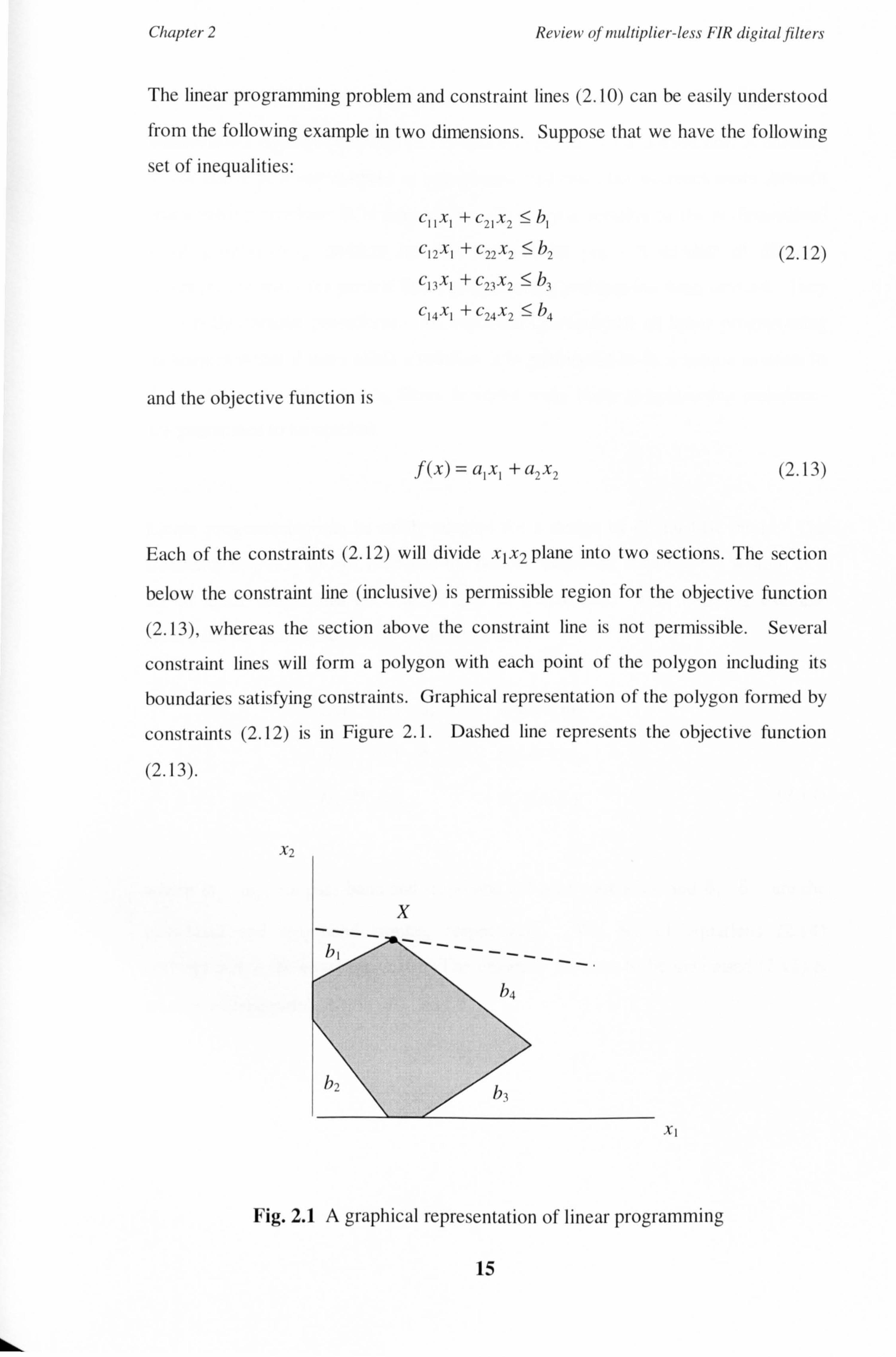
The linear programming problem and constraint lines (2.10) can be easily understood
from the following example in two dimensions. Suppose that we have the following
set of inequalities:
and the objective function is
Review u/ mirlliplicr--less /%R rligitul filze rs
Cl I XI +c21 x2 b,
CIA + c22x2 h2 (2.12) CIA +c23x2 b3
c14xI + c24x2 < h4
f(x) = u, x, +u2x2 (2.13)
Each of the constraints (2.12) will divide xIx2 plane into two sections. The section
below the constraint line (inclusive) is permissible region for the objective function
(2.13), whereas the section above the constraint line is not permissible. Several
constraint lines will form a polygon with each point of the polygon including its
boundaries satisfying constraints. Graphical representation of the polygon formed by
constraints (2.12) is in Figure 2.1. Dashed line represents the objective function
(2.13).
X2
XI
Fig. 2.1 A graphical representation of linear programming
15
bb..,

Chapter 2 Review of multiplier-less FIR digital filters
The objective here is to find values of {x; } which are within the polygon and
maximise the objective function (2.13) that is depicted by the dashed line. A solution
of the above problem is trivial in two-dimensional case, but becomes more difficult
when solving problems in N dimensions. An analytic solution to the N-dimensional
linear programming problem has not been found yet. A number of different
techniques to solve the general linear programming problem has been devised. They
are mostly iterative procedures. An important characteristic of linear programming
techniques is that if there exists a solution, it is guaranteed to be a unique solution to
the problem. In other words, filters designed using linear programming techniques
are guaranteed to be optimal.
Linear programming can be easily adapted for a design of digital FIR filters. The
frequency response of FIR filter and the desired frequency response are written as a
set of linear inequalities on a dense grid of frequencies. The following example
shows the set of inequalities for a low-pass filter:
H(e'w)51+51 0: 5 wSwP
H(e'w) _ 1-S, 0<_w<-wp
S2 cu, <_ (»: 5 7r (2.14)
where co,, 9 w, , are pass-band and stop-band cut-off frequencies, and 5 1,62 are the
pass-band and stop-band ripples, respectively. The set of equations (2.14)
corresponds to the equation (2.10). The objective function to be minimised (2.11) is
usually a linear combination of6, and S2.
16

Chapter 2 Review of multiplier-less FIR digital filters
2.2 Design techniques of multiplier-less linear-phase FIR digital
filters
Despite the large number of algorithms developed for the design and implementation
of infinite precision FIR filters, no closed-form design formulas for the multiplier-less
FIR filter design have been developed yet. The main methods for optimal FIR filter
design, such as the Remez exchange algorithm and linear programming, are not
suitable because they do not allow an inclusion of discrete coefficient set constraint.
Essentially, there are two possible approaches to the design of multiplier-less FIR
digital filters. We have denoted these approaches as algorithmic methods and
architecture-optimising methods.
The concept of algorithmic methods is to design multiplier-less digital filters with
discrete coefficients selected from the discrete domain of powers-of-two. Therefore,
a multiplication operation is converted to simple shift and add operations. As a result
of that, multipliers can be removed from the filtering structures. Algorithmic
methods are not limited to a particular filter structure and are suitable for any
implementation of the filtering structure (direct form, transposed form, cascades,
etc. ). Algorithmic methods are mostly iterative procedures based on the algorithms
which have been established as the main techniques in the design of FIR digital filters
with infinite precision coefficients.
A different design philosophy can be seen in architecture-optimising methods. These
methods attempt to optimise the hardware realisation of filtering structures so that
some (or all) of the multipliers can be removed. Architecture-optimising methods
include design of FIR filters using various number systems [Kin7l], recursive
architectures [Ram89], numerous arrangements of filter structures [Gre85, Sha87,
Sar9l, Bu191], systems with the filtering operation distributed in time and space
[Gha93], etc.
17

Chapter 2
2.2.1 Algorithmic methods
Review of multiplier-less FIR digital filters
Algorithmic methods focus on design of filter coefficients with lower complexity
rather than on the optimisation of hardware structures. This in turn leads to lower
implementation complexity of filtering structures. There are two categories of
algorithms to solve an approximation problem for FIR filters with powers-of-two
coefficients (PWR2): exact and approximate. Exact algorithms guarantee the optimal
filter design, i. e. a minimum order of the filter for a given specification. An example
of exact algorithms is an exhaustive search (examines all possibilities) and a branch-
and-bound algorithm [Lim83a]. Approximate algorithms do not guarantee the
optimality of the design, although they can deliver near-optimal designs in less time
than exact algorithms. The majority of algorithms for the multiplier-less FIR filter
design belongs to the category of approximate algorithms.
The following sections list and explain design methods and techniques used in the
design of multiplier-less digital filters as they chronologically appeared. Benefits and
restrictions for each method are explained.
2.2.1.1 Rounding of infinite precision filter coefficients
Rounding of infinite precision filter coefficients to nearest powers-of-two is the
simplest method for the multiplier-less FIR filter design. It is often used as a
benchmark to test performance of other more complex algorithms. The rounding
algorithm is relatively simple:
Step 1) obtain infinite precision filter coefficients for a given filter specification and
a given length of filterN by any of the methods described in 2.1.1,
18

Chapter 2 Review of multiplier-less FIR digital filters
Step 2) round the infinite precision coefficients to the nearest power-of-two (or a
sum/difference of two powers-of-two),
Step 3) evaluate the frequency response,
Step 4) if the frequency response satisfies the desired frequency response D(e3(')
then finish, otherwise increment the length of filter and go to the Step 1.
The advantage of this method is its simplicity and the possibility to utilise any of the
methods described earlier in the process of designing infinite precision coefficients,
thus allowing to choose a preferred approximation criterion. However, filters
designed by rounding of optimal infinite precision coefficients are not guaranteed to
be optimal. This is because of the fact that the domain of powers-of-two is not
searched for a solution. Instead, searching is conducted in the real domain and
subsequently mapped onto powers-of-two domain. In general, most of the methods
described below are able to design multiplier-less FIR filters with a smaller deviation
from the desired frequency response or fewer coefficients for a fixed error.
2.2.1.2 Mixed Integer Linear Programming
Linear Programming has been shown beneficial in the design of infinite precision FIR
filters (see section 2.1.1) as it is able to handle additional linear constraints.
Unfortunately, linear programming cannot be applied to the design of discrete
(PWR2) coefficient filters, since it does not allow the inclusion of this type of
constraint. When the coefficient domain is discrete and uniformly distributed, the
integer linear programming (ILP), an extension of linear programming techniques,
can be used. ILP techniques were successfully applied to the design of FIR digital
filters with integer coefficients to minimise finite wordlength (FWL) effects by Kodek
[Kod80].
19

Chapter 2 Review of multiplier-less FIR digital filters
The design problem is more difficult when considering FIR filters with powers-of-
two coefficients since powers-of-two are non-uniformly distributed. General integer
linear programming techniques cannot be used for optimisation in a domain that is
non-uniformly distributed, unless they are modified. Modified integer linear
programming techniques applicable to the design of FIR filters with PWR2
coefficients in the minimax sense has been first reported in [Lim79] and then
subsequently in [Lim82, Lim83a, Lim83b, Lim88, Lim90]. Lim proposed mixed
integer linear programming (MILP), a combination of ILP techniques with a branch-
and-bound algorithm, to solve the design problem in non-uniformly distributed
coefficient domain.
The branch-and-bound algorithm limits the number of solutions needing to be
examined by calculating upper and lower bounds on partial solution of the problem.
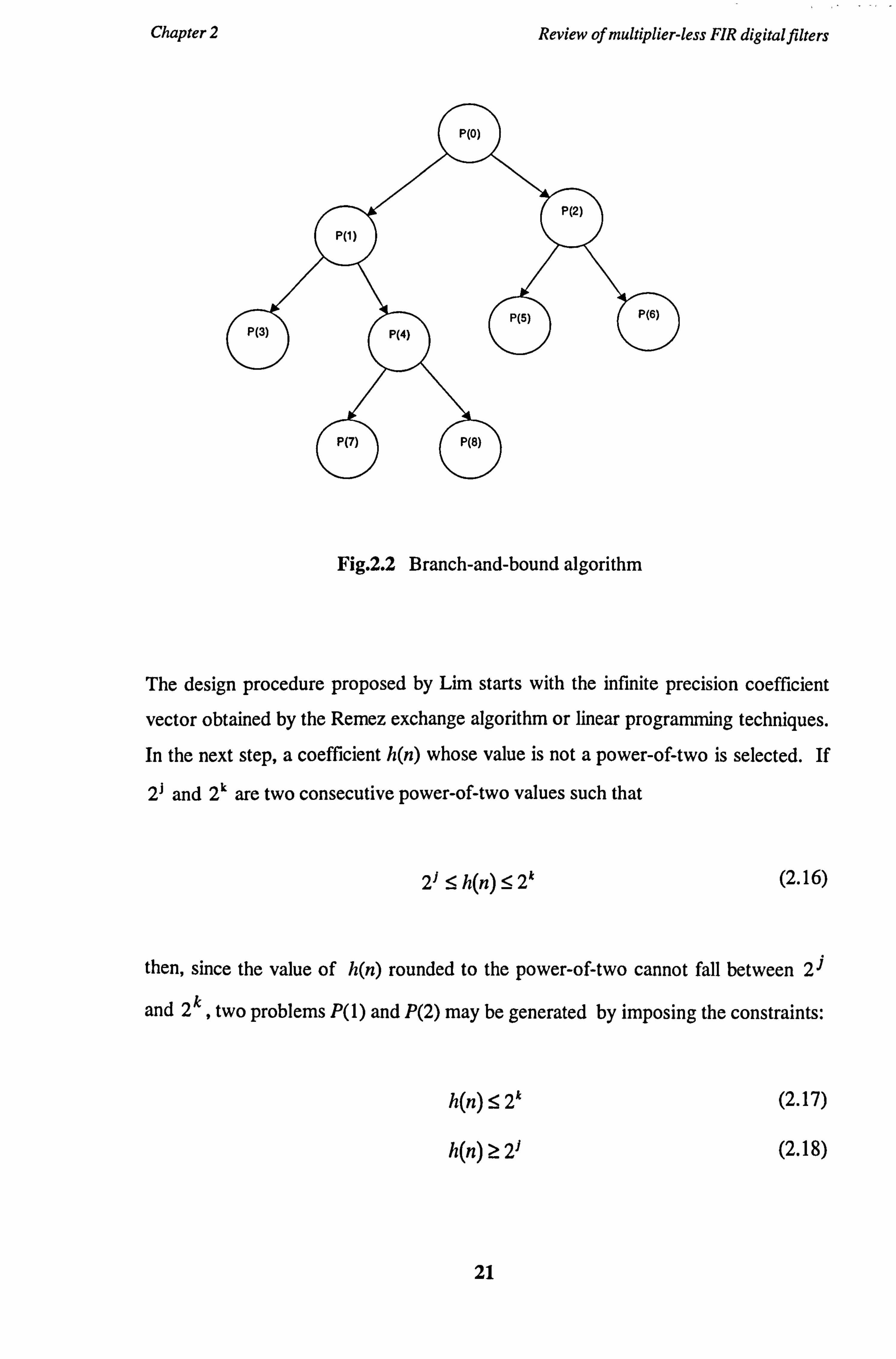
The algorithm creates an enumeration tree starting with an unsolved problem P(O).
A solution of the problem P(O) is S(O). The problem P(O) is resolved into smaller
problems P(i) with solutions S(i) satisfying the following condition:
Vi: u S(i) = S(0) (2.15)
This process is further continued by resolving subproblems P(i) into smaller
subproblems. Bounds are used to prune a search tree as the enumeration process
proceeds. The process continues until the problem P(O) is solved. An illustration of
Branch-and-bound algorithm is shown in Fig. 2.2.
20
hkhý.
Chapter 2 Review of multiplier-less FIR digital filters
Fig. 2.2 Branch-and-bound algorithm
The design procedure proposed by Lim starts with the infinite precision coefficient
vector obtained by the Remez exchange algorithm or linear programming techniques.
In the next step, a coefficient h(n) whose value is not a power-of-two is selected. If
2J and 2k are two consecutive power-of-two values such that
2f <_ h(n) 5 2k (2.16)
then, since the value of h(n) rounded to the power-of-two cannot fall between 2i
and 2k , two problems P(1) and P(2) may be generated by imposing the constraints:
h(n) S 2k (2.17)
h(n) > 2J (2.18)
21

Chapter 2 Review of multiplier-less FIR digital filters
as shown in Fig. 2.2. Problems P(1) and P(2) are solved individually and further
branching is performed on P(1) and P(2). The process of branching continues until
the problem P(O) is completely solved. The number of branches required can be
reduced by removing those branches, where no improvements can be predicted (only
subproblems with better subsolutions are selected for further branching).
The MILP algorithm is at the present the only known algorithm to guarantee the
optimal design of FIR filters with powers-of-two coefficients in the minimax sense, i. e. minimising a peak weighted error function in the frequency domain using:
max{W(w) " [D(co; ) - H(w; )]} (2.19)
O)i
If the LMS approximation is required, it can be achieved by minimising the mean
squared weighted error function:
1: 1'V(wt) - ID(col)
- H(cw1 )I2 (2.20)
coi
Minimising of (2.20) is an integer quadratic programming problem, which is also
capable to produce optimal designs.
Frequency responses of filters designed by the MILP algorithm have been shown
superior to those obtained by simply rounding of infinite precision coefficients
[Lim83a]. Unfortunately, a very high computation cost of the MILP algorithm
prohibits its practical application to the design of high-order PWR2 FIR filters. The
upper bound on the filter length was found to be less than 70 in order to converge in
reasonable times [Lim90].
22
Chapter 2 Review of multiplier-less FIR digital filters
The design of high-order PWR2 has been presented in [Lim83b]. This has been
achieved by incorporating the least mean square (LMS) criterion into the MILP
algorithm. The LMS approach can be also used to design FIR filters in the minimax
sense, approximating the minimax criterion by adjusting the least squares weighting.
PWR2 filters with the filter length N: 5 90 were realised. However, the LMS criterion
algorithm does not guarantee an optimal solution.
2.2.1.3 Local search
A useful alternative to the branch-and-bound algorithm, particularly when designing
high-order FIR filters with PWR2 coefficients is the local search algorithm. It has
been applied to the design of finite wordlength filters [Kod81], but can be also
applied to the design of PWR2 filters. The local search algorithm iteratively explores
a neighbourhood of a given starting point for improvements until a local optimum is
found. Hence, the local search algorithm requires a good choice of starting point and
a good searching strategy. A starting point is usually an infinite precision coefficient
vector obtained by the Remez exchange algorithm or linear programming.
There are generally two types of searching strategies:
a) changing each coefficient, one at a time, in both directions and repeating the
process until no further improvement is registered,
b) changing two or more coefficients over all possible pairs of coefficients, thus
allowing to analyse searching space in more extensive manner.
Local search can yield to substantial improvements of the frequency response when
compared with rounding of infinite precision coefficients to their nearest neighbours.
A performance of the local search can be severely reduced when the landscape of frequency response contains deep local minima, as local search tends to be easily
trapped in those minima.
23

Chapter 2 Review of multiplier-less FIR digital filters
2.2.1.4 Proportional relation-preserve/ simple symmetric sharpening method
A simple suboptimal algorithm for the design of PWR2 filters enabling sharp cut-off
frequencies and capable to design filters with filter length N> 200 was proposed by
Zhao and Tadokoro [Zha88]. The algorithm embodies two methods. The first
method is a suboptimal design that determines PWR2 coefficients from the set of
infinite precision coefficient vectors. The method, referred to as the proportional
relation-preserve (PRP) method, preserves a proportional relation between the
optimal infinite precision coefficients and the PWR2 coefficients. When filters
designed using the PRP method cannot satisfy given filter specifications, the second
method, referred to as simple symmetric-sharpening (SSS) method, is employed.
The PRP method minimises the maximum error with a constraint on coefficients h(n),
allowing coefficients to be single power-of-two or powers-of-two values only. The
design strategy is as follows:
(1) The infinite precision filter coefficients ho(n) are calculated by the Remez
algorithm.
(2) The filter gain A of the filter with PWR2 coefficients is determined by varying
the gain A from 0.5 to 1.0 to minimise error function E(A) :
(N-1)12 [A x h0(n)] 2
E(A) = I ho(n) -A (2.21) n=0
where the symbol [] represents rounding to PWR2 values: ± 2-p- ± 2-q.. A
set of coefficients hA(n), which minimisesE(A) of (2.21) is defined.
(3) The filter coefficients h(n) of the PWR2 filter are determined by local
optimisation to preserve, as far as possible, the proportional relation between the
24

Chapter 2 Review of multiplier-less FIR digital filters
coefficients ho(n) and h(n). This is accomplished by selecting the optimum
combination of nl adjacent coefficients hA(n) and n2 discrete values of these
coefficients to minimise the maximum error 5. The optimal values of nl and n2
have been experimentally found to be 4 and 5, respectively.
(4) The previous operation is carried out recursively for all coefficients and the
maximum error 5 is recorded.
(5) The same operation is continued using coefficient values obtained from the
previous operation as initial values. If the maximum error 8 is larger than error
in the previous operation, the local optimisation is stopped.
(6) If the designed filter does not satisfy the given specification on the maximum
error S, the filter length Nis incremented and the algorithm starts again.
The SSS method on the other hand, can greatly improve the approximation errors of
the PRP method. It is based on the sharpening of the frequency response of the
symmetric FIR filter by multiple use of the same filter, a technique described by
Kaiser in [Kai77]. The filter designed by the PRP method is considered as a subfilter
HS(z) of the filter H(z) designed by SSS method. The SSS method is applied when
the filter length N becomes greater than N,,, = 59.
2.2.1.5 Samueli's method
A technique of rounding infinite precision filter coefficients to their nearest power-of-
two values described in section 2.2.1.1 has been adopted by Samueli for the design of
multiplier-less FIR filters with the canonical signed-digit (CSD) coefficients [Sam88]. To define canonical signed-digit numbers, signed-digit numbers must be
explained first.
25

Chapter 2 Review of multiplier-less FIR digital filters
Signed-digit (SD) numbers were formally defined by Hwang [Hwa79]:
Given a radix r, each digit of an SD number can assume the following 2x+1 values:
(2.22)
r
where the maximum digit magnitudes must be within the following region:
r2 cc !5r -I (2.23)
II
In (2.23), the symbol rxl represents the smallest integer that is more than or equal to
the real number x. Because integer a must be bigger or equal to one, the minimum
radix r bigger or equal to two must be assumed.
The radix-r signed-digit representation of a fractional numberx has the general form
x=ýakr P.
k=1 (2.24)
where L is the number of nonzero digits, p. E {O, 1,..., B-1} determines positions of
nonzero bits and B is the total number of bits.
A minimal signed-digit representation that contains no adjacent nonzero digits ak is
called a canonical signed-digit representation. The CSD representation has some
interesting properties. For example, a number of adders/subtracters required to
realise a CSD coefficient is one less than the number of nonzero digits in the code.
The added redundancy and the added flexibility of negative digits allows most
26

Chapter 2 Review of multiplier-less FIR digital, filters
numbers to be represented with fewer nonzero digits. This can be used in the design
of totally parallel adders and fast hardware multipliers.
The starting point for the Samueli's algorithm is an infinite precision coefficient
vector obtained by the Remez exchange algorithm. Infinite precision coefficients are
scaled prior to rounding to avoid a possible overflow and also to minimise the error introduced by rounding. Scaled coefficients must satisfy a condition:
N-1
Ih(n)l :51. n=0
(2.25)
Samueli has found, that the best results are achieved when the filter coefficients are
scaled so that the largest coefficient can be represented exactly by two-bit CSD
coefficient. Scaled filter coefficients h(n) are rounded to the nearest sum or
difference of at most two powers-of-two and represented by a CSD numbers with at
most two nonzero bits. This resulted in at most one adder required to implement
each coefficient.
An improved, two-stage optimisation algorithm has been presented in [Sam89]. In
the first stage, a search for an optimum scale factor is performed. The algorithm
allocates one additional nonzero digit in the CSD representation to those coefficients
whose magnitudes exceed 0.5. This is to compensate for the very non uniform
distribution of the CSD coefficient set. When the optimum scale factor is found, a set
of infinite precision filter coefficients is scaled and rounded to the nearest CSD
coefficients.
The process of scaling and rounding of coefficients is followed by a bivariate local
search [Kod8l] in the neighbourhood of CSD coefficients. All possible pairs of
coefficients are varied by one quantisation step size in both directions and the
resulting peak ripple 8 is calculated. A coefficient vector resulting in the minimum
27

Chapter 2 Review of multiplier-less FIR digital filters
value of S is selected for further optimisation. The bivariate local search is repeated
with this coefficient vector as the starting point. The process of bivariate local search
stops when no further improvement is obtained. Filters with CSD coefficients
designed using Samueli's algorithm were found to have nearly optimal performances
when compared with the ideal infinite precision filters.
2.2.1.6 Coefficient sensitivity method
An improved optimisation algorithm based on Samueli's algorithm [Sam89] was
presented in [Sha9l]. The improved algorithm replaces a scaling procedure by
evaluating the sensitivity S� of the coefficients h(n) rounded to the nearest power-of-
two.
Prior to the optimisation procedure, the optimal infmite-precision coefficient vector is
obtained by one of the conventional design methods (Remez exchange algorithm or
linear programming). The optimisation procedure evaluates the sensitivity S� of the
frequency response to each of the coefficientsh(n).
The sensitivityS� is calculated as follows:
" each coefficient, in turn, is set to its nearest power-of-two, yielding in each case a 9 response An (co)
,
" the sensitivity is calculated as the sum of the increase in the pass-band ripple and
the increase in the stop-band ripple:
28

Chapter 2 Review of multiplier-less FIR digital filters
sn = (IAn
(w)Imax - IAn
(w)Imin )passband
- (IA((t')Imax -
IA((')Imin)
passband
+ An (0))Lax) - (IA(co)lmax )stopband
stopband
(2.26)
All coefficients are then set to their nearest power-of-two. If the frequency response
at this stage does not satisfy a prescribed specification, the coefficients are set one
after another, in the decreasing order of sensitivity, to the nearest sum or difference
of two powers-of-two. The frequency response is evaluated after each change of
coefficient and the entire process is repeated until the frequency response does not
satisfy a given filter specification. When all coefficients are changed and the given
filter specifications are not met, the design procedure may be repeated with an
increased filter length.
An alternative approach is to re-calculate the coefficient sensitivity S� with each
coefficient set to the nearest sum or difference of two powers-of-two. Then all
coefficients are set to the nearest sum or difference of two powers-of-two and the
frequency response is evaluated. If the frequency response is not within the
prescribed specification, the coefficients are set one after another, in the decreasing
order of sensitivity, to the nearest sum or difference of three powers-of-two. The
frequency response is evaluated at each stage and the optimisation procedure
continues until a satisfying frequency response is obtained.
The coefficient sensitivity method has been compared with other algorithms described
in the literature (rounding to the nearest power-of-two, Samueli's algorithm, etc. ).
Superiority of the improved algorithm has been demonstrated in terms of savings of
the number of PWR2 coefficients required to realise a given filter specification.
29

Chapter 2 Review of multiplier-less FIR digital filters
2.1.1.7 Design of multiplier-less FIR filters using genetic algorithms
Research into the design of multiplier-less digital filters using genetic algorithms has
been initiated by Suckley in [Suc9l]. Suckley described synthesis of FIR filter
structures by cascading of simple elements from a library of primitive filters. All
primitives in the library were computationally simple blocks with a multiplication
reduced to shift-and-add operations, hence producing multiplier-less FIR structures.
A genetic algorithm was used to select the best combination of primitives. Suckley's
method is a further development of integer linear programming techniques applied to
the synthesis of cascades of primitive elements described by Wade et al. [Wad90].
Recently, Wade et al. also reported a synthesis technique for multiplier-less FIR filter
design using genetic algorithms [Wad94]. A drawback of the above techniques is
that a filtering structure is determined at the same time as the filter coefficients.
Therefore filters designed using these methods are not suitable to implement with
direct or transposed filtering structures.
Schaffer et al. presented a software tool Fil-E using a genetic algorithm to evolve
digital filters with PWR2 coefficients [Sch93]. The approach used in Fil-E to design
ML FIR filters is similar to that of Suckley's and Wade's work: cascades of FIR
filters. Schaffer suggests that the 3-stage cascades are suitable for most designs. If
the frequency response is not within the specified boundaries, either the number of
cascades or number of coefficients in each cascade is changed and a population of
filter structures is re-evaluated. Fil-E uses Gray coding with only four bits to encode
PWR2 coefficients onto chromosomes. To estimate the order of the filter, heuristics
formulas used for the design of infinite-precision coefficients have been applied.
Gentilli et al. described an evolutionary design of ML FIR filters that introduces the
pass-band gain G criterion [Gen94] as the additional parameter of the optimisation
problem. The pass-band G preserves a proportionality between the power-of-two
and infinite-precision coefficients similar to that described by Zhao et al. in [Zha88].
The pass-band gain G is relevant when rounding infinite-precision coefficients to
30

Chapter 2 Review of multiplier-less FIR digital filters
powers-of-two using heuristics methods, yet it limits searching space for the genetic
algorithm.
2.2.2 Architecture-optimising methods
Architecture-optimising methods focus rather on the optimisation and implementation
aspects of filter structures than on the design and optimisation of filter coefficients.
They are usually associated with specific architectures, what does not make them
very practical when considering, for example, implementation of digital filtering
algorithms using digital signal processors (DSP).
One of the first multiplier-less architectures was proposed by Greenberger [Gre85]
and improved by Shah [Sha87]. It was achieved by rearranging the order of
convolution operations so that the convolution has been replaced with simple SHIFT
and ADD operations. Although the proposed architecture is multiplier-less, the final
number of gates was approaching the complexity of filter structures using multipliers.
In addition, the proposed arrangement does not have an advantage of higher speed
than multiplier based filter structures.
Filter structures using the logarithmic system [Kin7l] do not require multipliers as
the multiplication of two operands is achieved by adding their logarithms. On the
other hand, the addition operation is fairly complex and there is also a need to
convert numbers between binary and logarithmic representations.
It has been observed that better frequency responses can be achieved by multiple use
of the same filter. This has been described by Kaiser et al. as the Amplitude Change
Function (ACF) technique [Kai77]. Ramakrishnan et al. [Ram89] adopted this
technique for the multiplier-less filter design by choosing a recursive running sum
(RRS) filter as the prototype filter for cascading. As a result, their filter structure
uses fewer multipliers and adders. However, the number of delay units has doubled
31

Chapter 2 Review of multiplier-less FIR digital filters
when compared to conventional methods and the technique assumes a prefixed filter
architecture.
Tai et al. has further improved Ramakrishnan's technique by using the cascade of a
cosine function (CCOS) as the prototype filter [Tai92]. The resulting filter structure
in [Tai92] does not use any multipliers. However, this method also assumes a
prefixed architecture for the filter implementation.
Other multiplier-less filter design approaches include the use of primitive operators
described by Bull et al. [Bu187, Bu188, Bu191], or periodically time-varying state-
space structures (PTV-SS) distributing the filtering operation over space and time.
The principle of the primitive operator method exploits the redundancy in the direct-
form filter structure. This has been achieved by decomposition of each product in the
convolution operation into a number of primitive arithmetic operations and reusing of
partial results to form other product terms.
The use of periodically time-varying state-space structures using ternary coefficients
({0, ±1)) and therefore multiplier-less, has been described by Ghanekar in [Gha93].
Because PTV-SS structures use upsampling and downsampling and therefore
effectively operate at N times the input signal rate, where N is the rate of upsampling,
they are not practical for high-speed applications. The PTV-SS structures are
applicable also to the design of multiplier-less IIR filters [Gha94].
32
Chapter 2 Review of multiplier-less FIR digital filters
2.3 Conclusion
A number of design techniques and algorithms used for the design of multiplier-less
digital filters have been presented. Each method has its advantages and
disadvantages. For instance, architecture-optimising methods are generally not
suitable for software implementation. Some of these architectures need a special
hardware to convert between different number systems. However, they do not need
specific algorithms for the design of filter coefficients, as they can usually operate
with Remez coefficients.
Algorithmic methods are not limited by implementation issues. They use infinite
precision coefficients calculated by Remez algorithm as an initial coefficient vector
and iteratively search for a coefficient vector that is composed from power-of-two
terms only. Apart from mixed integer linear programming incorporating the branch-
and-bound algorithm, and the enumerative search, which is not practical, they are not
optimal in the minimax sense. To date, the MILP algorithm developed by Lim is the
only method that guarantees an optimal solution in minimax sense. However, the
MILP algorithm is not practical for higher order filters as the computational cost
becomes excessive. The summary of the algorithmic methods is in Table 2.1.
We conclude this chapter with the observation that Shaffeu et al. [Sha91] presented a
method that outperformed other classical techniques used in multiplier-less FIR filter
design. Shaffeu's method is simple, it has a relatively short design time when
compared to MILP and authors claim that a minimum filter length required to satisfy
the desired frequency response is shorter than with other methods. We will analyse
this method in more detail and investigate further improvements in the next chapter.
33

Chapter 2 Review of multiplier-less FIR digital filters
Table 2.1 Algorithmic methods for the multiplier-less digital filter design
Method Initial set of Optimal Max. length of Features and
coefficients filter N limitations
Rounding Remez No unlimited simple
(nearest PWR2)
MILP Remez Yes N :: g 70 to date this is the
(branch-and- only optimal bound)
method
MILP Remez No N <_ 90
(LMS criterion)
Local search Remez No
PRP/SSS Remez No N<_59 (PRP method
only)
N>200
(PRP+SSS)
Samueli's Remez No uses CSD
method coefficients
Coefficient Remez No not limited produces best sensitivity results from non- method
opt. methods
34

Chapter 3
Novel techniques of multiplier-less FIR
filter design
This chapter presents two novel design methods for ML FIR digital filters based on
classical design methods. First, a modification of a local search algorithm, an
evolutionary local search is described [Cem93c]. The evolutionary local search is
very simple, but it can produce better results than simple rounding of infinite
precision coefficients to nearest power-of-two numbers. An advantage of the
evolutionary local search is that there is no need to calculate Remez coefficients.
The rest of this chapter is devoted to two novel algorithms based on Shaffeu's
method of rounding of filter coefficients based on coefficient sensitivity. The first
algorithm is an improvement of the coefficient sensitivity criterion for filters with
multiple bands. The improved sensitivity criterion yields better frequency responses
and lesser complexity of filter coefficients (i. e. more coefficients are represented as
35

Chapter 3 Novel techniques of multiplier-less FIR filter design
single PWR2 and less coefficients as 2PWR2). The second algorithm replaces
Shaffeu's sensitivity criterion with a novel sensitivity criterion that is based on a mean
square error (MSE) or a mean absolute error (MAE). The novel coefficient
sensitivity criterion yields better frequency responses and lesser complexity of
coefficients for all types of filters, including filters with multiple bands. The most
significant contribution of the novel sensitivity criterion is that it can result in shorter
filter lengths than the original Shaffeu's criterion. A shorter filter length represents a
number of advantages, e. g. shorter design times, lesser complexity and a smaller
group delay.
3.1 Evolutionary local search
A modification of the local search algorithm, an evolutionary local search (ELS), is
presented in this section. The evolutionary local search for the design of multiplier-
less FIR filters uses sequential and modified sequential searching methods. The
minimum solution is acquired from a set of power-of-two coefficients and does not
pre-empt the filter architecture prior to the calculation of the coefficients, thus
supporting a variety of alternative implementations. It also eliminates the use of
sensitivity procedures to map real coefficients to their nearest power of two
coefficients as no standard procedure is used to obtain the initial real coefficients.
Evolutionary local search guarantees the optimal solution for low-order filters and
suboptimal for higher orders.
An alternative approach to the Remez-based technique could search for a suitable
coefficient vector from the possible arrangement of the values over the range defined
by the coefficient wordlength. This suggestion is impractical as the complexity of the
searching process increases beyond the capability of existing computing machines.
However, since we are interested in multiplier-less FIR filters, the restriction of the
coefficients to power of two values reduces dramatically the number of possible
arrangements of coefficients.
36

Chapter 3 Novel techniques of multiplier-less FIR filter design
The proposed coefficient approximation procedure uses the following concept.
Initially, a basic set of possible power of two coefficients is defined. The band
tolerances are then entered, and the minimum length filter is evaluated using Kaiser's
formula. Starting from this order, all possible arrangements of coefficients extracted
from the basic set have their frequency responses computed and compared with the
desired frequency response. When a satisfactory solution is obtained, the algorithm
terminates, otherwise the next arrangement is used until all combinations have been
evaluated. When no solution is found, the order of the filter is increased and the
process is repeated. The nature of this sequential search guarantees minimum order
multiplier-less filters.
For more complex filters that require a large number of coefficients to approximate
the desired frequency response, this method has shortcomings due to the excessive
amount of computations resulting from the complexity of the search process. A
modified procedure is proposed for these categories. The pseudo-code of the
modified procedure is illustrated in Figure 3.1. The source code written in Pascal is
included on the accompanying disk.
The minimum length is evaluated again by Kaiser's formula and the coefficients'
values randomly assigned. The procedure searches through all possible powers of
two for the best value for each coefficient. The value that provides the best
frequency response approximation is saved and the procedure continues with the next
coefficient. This procedure is repeated until no further improvements in the
approximation of the desired frequency response are obtained. If no solution is
found, the order of filter is increased and the process repeated. This approach adopts
the principle of keeping the best and rejecting the rest through sequential exchange.
The method is faster than the sequential searching, and computer simulations have
shown better results compared to conventional methods of simple rounding (SR) to
nearest power-of-two.
37

Chapter 3
Evolutionary local search ()
begin
Novel techniques of multiplier-less FIR f lter design
evaluate the minimum length of filter
initialise coefficient values randomly
repeat
for each coefficient do
search all PWR2 values
evaluate frequency response
keep the best coefficient
end for
if unsatisfactory frequency response then
increment the length of filter
end if
until satisfactoryfrequency response
end
Fig. 3.1 Pseudo-code of the evolutionary local search
A more powerful method that produces better results can be obtained when the
discrete space of the coefficients to be explored is extended. This is done by a small
variation of the searching procedure when the coefficients are arranged into groups
of two or three. Thereafter, all possible combinations of powers of two terms for
each group of coefficients are explored. There are three possible modes of
arrangements of these coefficients into groups: randomly, sequentially and according
to their fitness. The arrangement of the coefficients that gives the least mean square
error in the frequency response is saved and the searching procedure continued with
another group of coefficients.
The evolutionary local search (ELS) algorithm has been compared with the
conventional rounding of infinite precision coefficients. The conventional rounding
38

Chapter 3 Novel techniques of multiplier-less FIR filter design
method uses McClellan - Parks algorithm to obtain an initial set of coefficients and
then this set is approximated to the nearest power of two coefficients. The ELS
algorithm is shown to produce superior results to the more conventional approach.
Results obtained using the evolutionary local search algorithm are compared to the
conventional rounding to nearest power-of-two coefficients in Table 3.1. Typical
frequency responses for filters from Table 3.1 are shown in Figure 3.2.
Table 3.1 Comparison between simple rounding (SR) to the nearest PWR2 and
evolutionary local search (ELS) algorithm
Filter Frequency Desired Max. error Filter Filter Coeffs.
No. Bands response allowed Length Length saving
(SR) (ELS)
0-0.05
1 0.20-0.30 band-pass 0.1 13 13 0
0.45-0.50
0-0.30
2 0.45-0.50 high-pass 0.1 15 11 27 %
0-0.25
3 0.37-0.50 low-pass 0.15 14 8 43 %
0-0.30
4 0.45-0.50 low-pass 0.1 10 8 20 %
0-0.10
5 0.20-0.30 band-pass 0.2 13 10 23 %
0.40-0.50
39

Chapter 3 Novel techniques of multiplier-less FIR filter design
Pass-band region
0.05 0.1 0.15 0.
vv0 0.1 0.2 0.3 0.4 Normalised Frequency
(a) frequency response of the filter No. 3
10
0
-10
-20
m -30
-40
-50
-60
-70
_un
0
-20
-40
-60 v S _ -80
-100
-120
-i do
Pass-band region
.2
-4
-6
-8
. tp 0.05 0.1 0.15 02 0.25 0.3
Tv0 0.1 0.2 0.3 0.4 0.5 Normalised Frequency
(b) frequency response of the filter No. 4
Fig. 3.2 Comparison of simple rounding (SR) and evolutionary local search (ELS)
40
Chapter 3 Novel techniques of multiplier-less FIR filter design
Figure 3.2 (a) depicts the frequency responses for the filter No. 3 with the solid line
representing the conventional method and the dotted line representing the ELS
algorithm. Both frequency responses are well within the specification, however, the
filter designed using the ELS algorithm requires only eight coefficients in comparison
with fourteen coefficients required when the conventional method of infinite-
precision coefficients is used. This represents 43% saving in the number of
coefficients. Figure 3.2 (b) shows the frequency responses for the filter No. 4. While
the saving in terms of the number of coefficients required is less (20%), the filter
designed using the ELS algorithm has better attenuation in the stop-band than the
filter designed using the conventional approach.
The ELS algorithm is applicable to any filter type, and because it does not assume a
prefixed architecture for the implementation, it could be implemented on any
processor that can perform a Multiply-Accumulate function. Furthermore, the
elimination of multipliers makes the resulting structure ideal for fast, low area, high
throughput rate ASIC implementations.
41

Chapter 3 Novel techniques of multiplier-less FIR filter design
3.2 Rounding of filter coefficients based on coefficient sensitivity
3.2.1 Coefficient sensitivity
The coefficient sensitivity reflects the degree of influence on the frequency response
of digital filter resulting from rounding of infinite precision coefficient to the nearest
power-of-two. The sensitivity of each coefficient as defined by Shaffeu in [Sha9l]
was calculated as the sum of the increase in the pass-band and stop-band ripples:
Sn = (IA,
w)i - IAn (w)l
min) passband
-(IA(co)l - IAcw>Imin )Passband
Passbund
+1 ,,
((0)lmaa )
smpband -
`IA(O)Imax
)slopband
where A(w) is the amplitude response of infinite precision coefficient vector and
A�(co)is the amplitude response with n-th coefficient changed to the nearest power-
of-two. As we will show later, this sensitivity measure does not yield a minimum
number of canonical coefficients (having more than one power-of-two term). It is
also not suitable for the design of multiple-band filters with power-of-two
coefficients. This is because in equation 3.1 the sensitivity is calculated using only six
extremes of the frequency response, ignoring extremes in different bands.
3.2.2 Modified coefficient sensitivity
We propose two novel approaches for the evaluation of the sensitivity criterion, both
maximising the number of single power-of-two coefficients and therefore reducing
the overall complexity of the filter. The first approach is a generalised version of the
sensitivity criterion in (3.1). The sensitivity is calculated using local maxima and
minima in each band, while Shaffeu used only global extrema. The improved
coefficient sensitivityS� is calculated as follows:
42

Chapter 3 Novel techniques of multiplier-less FIR filter design
Sn- ýj Ani (co)! max
- IAni (O)l
min /Passband i=1
-`IA(o !,,
- (A(0)Imin
)Passband (3.2)
N
+J: ([4,:
i (CO
),,
t,, pb.,, d -
`IA((o)lmax
)stopband
j=1
where NN and Ns represent the number of pass-bands and stop-bands, respectively.
The improved sensitivity criterion (3.2) has been shown superior to the original
sensitivity criterion (3.1), when designing PWR2 filters with multiple bands. Its
performance has been verified on several filter designs. Examples of the filter
specifications (band-pass and multiple-band filters) that have been used to evaluate
the performance of the modified sensitivity criterion are given in Table 3.2.
Comparisons of frequency responses for the band-pass filter BP1 are illustrated in
Figures 3.3 (a) and 3.3 (b), respectively. Solid lines represent frequency responses of
filters that have been designed using the original sensitivity measure, while frequency
responses of filters that have been designed using the improved criterion are
represented by the dashed line. Solid and dashed lines in Figure 3.3 (a) and 3.3 (b)
are aligned as frequency responses for both methods are approximately the same.
However, the design based on the improved sensitivity criterion cuts the total number
of canonical coefficients by 4 %. This results in a lower complexity of the filter
implementation.
Figures 3.3 (c) and 3.3 (d) show frequency responses of the filter with multiple bands
(example MB1). The improved sensitivity criterion resulted in smaller errors in the
pass-bands and slightly increased errors in the stop-bands. However, the number of
canonical coefficients has been decreased by more than 30 %. The results comparing
the minimum filter length and the total number of single PWR2 coefficients that are
required to satisfy frequency response constraints are summarised in Table 3.3.
43

Chapter 3 Novel techniques of multiplier-less FIR filter design
Table 3.2 Examples of filters designed using modified sensitivity criterion
Filter type Number of Cutoff Desired Attenuation Maximum error
bands frequencies freq. resp. [dB] allowed
(f) (D) (6)
Bandpass 3 0-0.22, 0, > -26 dB 0.05,0.03,0.05
BP1 0.24-0.26, 1,
0.28-0.5 0
0-0.05, 1, 0.1,
Multiple bands 6 0.10-0.15, 0, 0.1,
MB1 0.20-0.23, 1, 0.1,
0.27-0.30, 0, 0.1,
0.35-0.4, 1, 0.1,
0.45-0.5 0 0.1
Multiple bands 0-0.04, 1, 0.1,
MB2 7 0.08-0.12, 0, 0.1,
0.16-0.22, 1, 0.1,
0.245 - 0.275, 0, 0.1,
0.30-0.34, 1, 0.1,
0.38-0.42, 0, 0.1,
0.46-0.5 1 0.1
Lowpass 2 0-0.27, 1, 0.02,
LP1 0.31-0.5 0 0.02
Lowpass 2 0-0.24, 1, 0.05,
LP2 0.25-0.5 0 0.05
44

Chapter 3 Novel techniques of multiplier-less FIR filter design
H (F)
1.5
0.5
0 0.1 0.2 0.3 0.4 0.5
F
(a)
0.5
0 0.1 0.2 0.3 0.4 0.5
H [dB]
50
-50
-100 0 0.1 0.2 0.3 0.4 0.5 F
(b)
H [dB]
(c) (d)
Fig. 3.3 Comparison of the original and improved sensitivity criterion:
(a) frequency response of band-pass filter BP1,
(b) as (a), but in logarithmic scale,
(c) frequency response of the multiple-bands filter MB 1,
(d) as (c), but in logarithmic scale.
45

Chapter 3 Novel techniques of multiplier-less FIR filter design
Table 3.3 Comparison of the original and improved sensitivity criterion
Filter Filter length Number of canonical coeffs.
with the criterion: with the criterion:
original improved original improved
BP1 74
MB1 31
74
31
50
17
48
11
MB2 41 41 39 23
3.2.3 Mean square error and mean absolute error sensitivity criterion
Although the sensitivity criterion (3.2) reflects the changes in the frequency response
for each band, it still overlooks the fact that by approximating infinite precision
coefficients with power-of-two terms, the entire frequency response is influenced at
more than few isolated points. Therefore, we propose a novel sensitivity criterion,
based either on a mean square error (MSE) or on a mean absolute error (MAE).
Both criteria make use of the entire information acquired within the process of
searching for extrema of the frequency response. The MSE criterion is more suitable
for the design of noise separating filters as the energy of signal is related to the square
of the signal. The MAE criterion can be used when a minimax design is preferred.
As we will show later in this section, MSE and MAE based sensitivity criteria
maximise further the number of coefficients that are single power-of-two [Cem93a].
Better interpretation and visualisation of the coefficient sensitivity as proposed by
Shaffeu in [Sha9l] can be achieved by re-arranging individual sensitivity terms in
equation 3.1. The re-arranged sensitivity criterion Sn is given as follows:
46

Chapter 3 Novel techniques of multiplier-less FIR filter design
S. =Jn (w)I. - IA(w)l, )Psbd
+(IA(w)Imin - IAn (° )Passband
Passband
" "ý sropband
where A(co) is the infinite precision coefficients' frequency response, and A'. (CO) is
the frequency response with the n-th coefficient changed to the nearest power-of-
two. The first term in (3.3) represents the difference between maximum ripples in the
pass-band for a filter with infinite precision coefficients and a filter with the n-th
coefficient changed to the nearest power-of-two. The second term represents the
difference between the smallest errors in the pass-band. The last term depicts the
difference between maximum ripples in the stop-band. Graphic interpretation of
individual sensitivity terms is illustrated for a low-pass filter in Figure 3.4.
IAI (ei(o)
1.2 r ý., ýý...... ..............
first term
] \\J/.. second term
........ .... ............ ......
0.8 \ \A, n
A 0.6
0.4
0.2 third term
4 """" ........
0 0.1 0.2 0.3 0.4 0.5
Normalised frequency
Fig. 3.4 Graphic interpretation of sensitivity
47

Chapter 3 Novel techniques of multiplier-less FIR filter design
Because the sensitivity is calculated using the global extrema in both bands, it is
necessary to seek their location across the whole frequency range. When searching
for maxima and minima in (3.1) and (3.2), the frequency response at each discrete
frequency point is evaluated. Except for the global extrema, this information is later
disregarded. In fact, the calculation of coefficients' sensitivity does not consider that
rounding of infinite precision coefficients to nearest powers-of-two influences the
frequency response across the whole range and not only in extrema points.
The MSE sensitivity criterion is based on the mean square error between the
frequency response of the filter with infinite precision coefficients and the frequency
response of the filter with the n-th coefficient changed to the nearest power-of-two.
The MSE criterion embodies every discrete frequency point across the entire
frequency range that has been evaluated. The MSE coefficient sensitivity is
calculated as follows:
SMSE(n)= L [An'(wi)-A(w; )]2 (3.4)
L , _,
Equally, the MAE criterion is based on the mean absolute error between the
frequency response of the filter with infinite precision coefficients and the frequency
response of the filter with the n-th coefficient changed to the nearest power-of-two:
L SMAE(n)
= (3.5) L ; _t
where CO, is a set of discrete frequency points:
fS ý' 0' 2N' 2N ' 2N "', wP, ws,.... 0.5 (3.6)
{Nft2. Nft 3"N
48

Chapter 3 Novel techniques of multiplier-less FIR filter design
where cop, co, are normalised pass-band and stop-band cut-off frequencies,
respectively and L is the number of discrete frequency points for evaluating the
frequency response given as:
2N"wp [2N. (o. 5_w) N13 Nfs
In equation (3.7), N represents the length of filter and Nfs is the size of desired
frequency step. The symbol LxJ means an integer less than or equal to the real
number x. By varying Nfs we can adjust the precision for the calculation of the mean
square error or the mean absolute error. The pseudo-code of the improved design
algorithm is shown in Figure 3.5, while the Matlab source code is included on the
accompanying disk.
49

Chapter 3 Novel techniques of multiplier-less FIR filter design
Rounding of filter coefficients based on coefficient sensitivity ()
begin
read initial specification of filter
repeat
calculate infinite precision coefficients
evaluate frequency response
choose criterion (MSE or MAE)
/* evaluate sensitivity of each coefficient using MSE(MAE) criterion
for each coefficient do
round i-th coefficient to PWR2
evaluate frequency response with changed i-th coefficient
calculate sensitivity Si
end for
/* round to the nearest PWR2 */
round all coefficients
repeat
evaluate frequency response
if unsatisfactory frequency response then
/* round to the combination of two PWR2 */
round next coefficient with the highest sensitivity
end if
end
until satisfactory frequency response
increment filter length
until satisfactoryfrequency response
Fig. 3.5 Pseudo-code of the rounding algorithm using the improved sensitivity
50
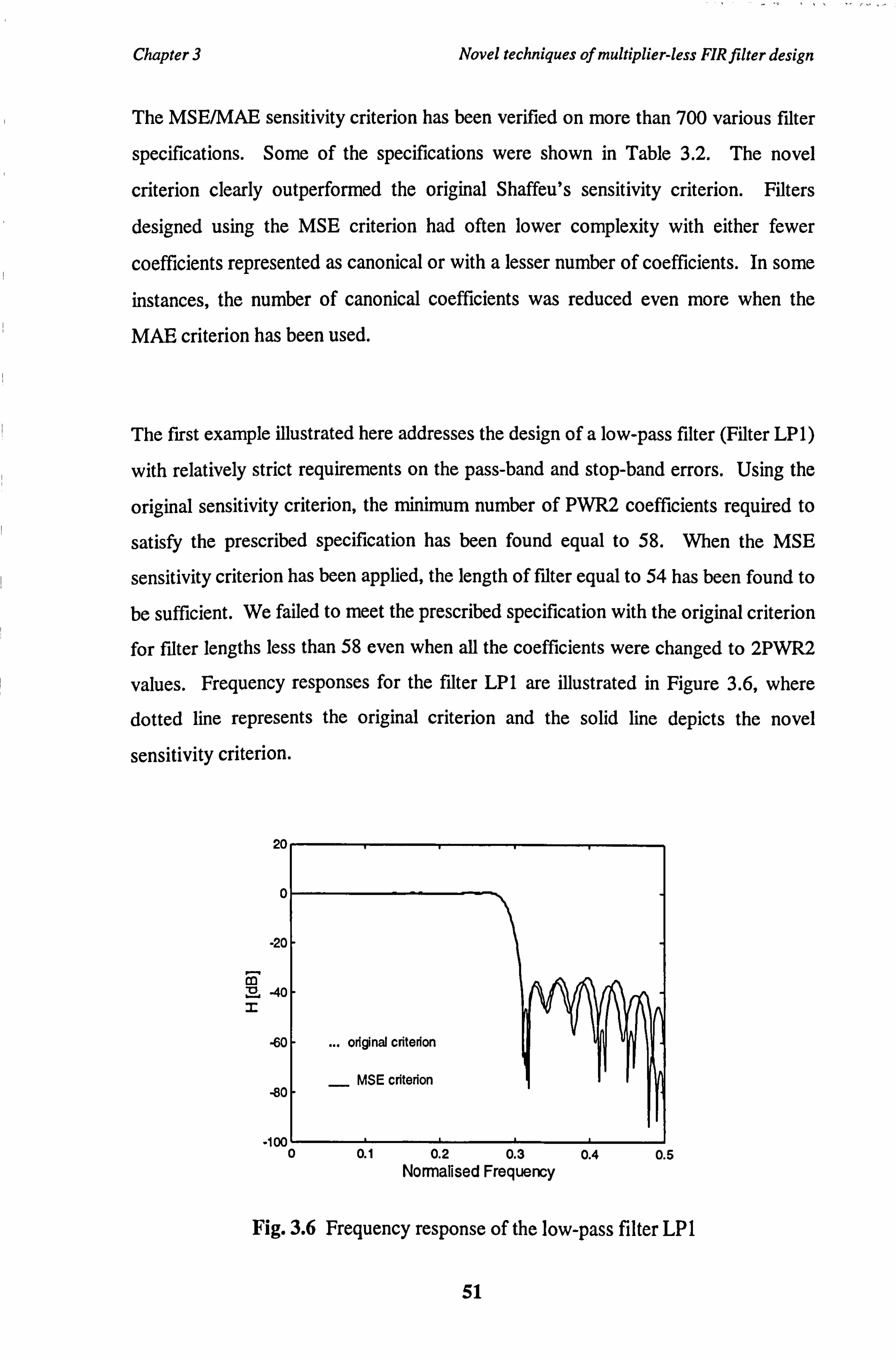
Chapter 3 Novel techniques of multiplier-less FIR filter design
The MSE/MAE sensitivity criterion has been verified on more than 700 various filter
specifications. Some of the specifications were shown in Table 3.2. The novel
criterion clearly outperformed the original Shaffeu's sensitivity criterion. Filters
designed using the MSE criterion had often lower complexity with either fewer
coefficients represented as canonical or with a lesser number of coefficients. In some
instances, the number of canonical coefficients was reduced even more when the
MAE criterion has been used.
The first example illustrated here addresses the design of a low-pass filter (Filter LP1)
with relatively strict requirements on the pass-band and stop-band errors. Using the
original sensitivity criterion, the minimum number of PWR2 coefficients required to
satisfy the prescribed specification has been found equal to 58. When the MSE
sensitivity criterion has been applied, the length of filter equal to 54 has been found to
be sufficient. We failed to meet the prescribed specification with the original criterion
for filter lengths less than 58 even when all the coefficients were changed to 2PWR2
values. Frequency responses for the filter LP I are illustrated in Figure 3.6, where
dotted line represents the original criterion and the solid line depicts the novel
sensitivity criterion.
20
0
-20
m
-40
-60
-80
-100 0 0.1 0.2 0.3 0.4 0.5 Normalised Frequency
Fig. 3.6 Frequency response of the low-pass filter LP 1
original criterion
- MSE criterion
51

Chapter 3 Novel techniques of multiplier-less FIR filter design
The next example illustrates the design of low-pass filter (Filter LP2) with very
narrow transition band, where the MSE sensitivity criterion failed to deliver expected
results. This can be caused by the fact, that the amplitude of ripples attributed to the
narrow transition band is averaged with other ripples when using the mean square
error approach. This is not the case of the original sensitivity criterion that
emphasises maximum error peaks. Bearing this in mind, we can conclude that in the
majority of cases the mean square error sensitivity criterion is superior to the original
sensitivity criterion proposed by Shaffeu. Frequency responses for the filter LP2 are
illustrated in Figure 3.7. They are almost aligned as there was very small difference
between both responses. However, the minimum number of coefficients when using
the MSE criterion has been found to be higher.
1c
-1
-2
U-3 v X-4
-5
-61
. 71
-80 0 0.1 0.2 0.3 0.4 0.5 Normalised Frequency
Fig. 3.7 Frequency response of the low-pass filter LP2
Results for all five filter examples using the original , MSE and MAE criteria are
summarised in the Table 3.4.
0.4
52

Chapter 3 Novel techniques of multiplier-less FIR filter design
Table 3.4 Comparison of Shaffeu's and novel (MSE based) sensitivity criterion
Filter Filter length Single PWR2 coe fficient Shaffeu MSE MAE Shaffeu MSE MAE
BP1 74 74 74 24 28 28 MB 1 31 31 31 14 20 20 MB2 41 41 41 2 18 18 LP1 58 54 54 16 18 18 LP2 133 141 141 82 64 39
3.3 Conclusion
In this chapter, we analysed the problem of designing multiplier-less digital FIR
filters. We presented three novel algorithms that are based on classic rounding of infinite precision filter coefficients. They include evolutionary local search, modified
coefficient sensitivity and mean squared error coefficient sensitivity for rounding filter
coefficients, respectively. These algorithms outperformed their counterparts and the
results are particularly encouraging for the MSE based method for rounding filter
coefficients.
However, there are still number of issues that have not been addressed. For instance,
the design of filters with phase requirements other than linear cannot be realised in a
straightforward manner. The algorithms are not suitable for the design of IIR digital
filters and they cannot guarantee the optimal design in the minimax sense. In fact,
none of the algorithms previously described can guarantee that the coefficients are
optimal (except the exhaustive search and mixed integer linear programming). Let us
summarise the observations and draw some conclusions for the multiplier-less FIR
filter design.
53

Chapter 3 Novel techniques of multiplier-less FIR filter design
(i) The algorithms presented in previous chapters are essentially searching
algorithms approximating infinite-precision coefficients by the discrete
coefficients (powers-of-two) that would satisfy the desired frequency response.
They use either the Remez algorithm or linear programming to obtain the initial
infinite-precision coefficient vector and they explore only the vicinity of
infinite-precision coefficients.
(ii) The set of discrete filter coefficients obtained by rounding of infinite-precision
coefficients is suboptimal. This is because the Remez algorithm and linear
programming methods can design filters that are optimal in the minimax sense
only with infinite-precision coefficients. By approximating these coefficients
with powers-of-two, we are ignoring a vast searching space where potential
optimal filter designs might occur. We still know very little about properties of
filters with power-of-two coefficients and no closed analytical solutions for the
design of multiplier-less filters with powers-of-two coefficients have been
developed yet.
(iii) Essentially, the problem of discrete coefficient filter design is a combinatorial
optimisation problem of an enormous computational complexity. For example,
let us consider a design of linear-phase FIR digital filter with 50 coefficients,
using 16 bit wordlength. By restricting the coefficients to single power-of-two
numbers and reserving one bit as a sign bit, we have 30 possible values for each
coefficient. Because of the symmetry of the impulse response, the number of
unknown variables is halved from 50 to 25. To find an optimal coefficient
vector, we are dealing with the 25-dimensional combinatorial optimisation
problem. The total number of coefficient combinations is given as:
C= Bw2 = 3025 = 8.472886.1036 (3.7)
54

Chapter 3 Novel techniques of multiplier-less FIR filter design
where B is the number of all possible discrete values for each coefficient and N is
the length of filter.
Imagine now, that we have extremely powerful computer facilities able to
calculate the frequency response and to evaluate one combination of coefficients
each picosecond. The time t that is needed to evaluate all combinations would
be
8.472886.1036 1=8.4 . 1024 sec = 2.7.10" years !!! Ps
Simple analysis of (3.7) will show that the time t increases exponentially with increasing filter length N. When the filter coefficients would be sums/ differences
of two (or more) power-of-two numbers, the total number of combinations
would be even bigger. Problems where the computing cost increases
exponentially with the dimension of the problem are in complexity theory
denoted as NP-complete problems (non-deterministic polynomial time complete
problems). For solving of NP-complete problems we need robust searching
algorithms that will handle combinatorial optimisation problems efficiently.
Natural algorithms, primarily genetic algorithms, offer themselves as ideal candidates.
They are powerful searching and optimisation algorithms, based on natural processes
and systems. An advantage of genetic algorithms is that the computing cost of GA's
grows linearly with the size of problem. Therefore we suggest that the kernel of
techniques for the design of ML FIR filters should be based upon natural algorithms,
primarily genetic algorithms. In the next chapter, we will show how genetic
algorithms can be applied to the design of multiplier-less FIR digital filters.
55

Chapter 4
Design of multiplier-less FIR filters
using genetic algorithms
This chapter presents a new robust technique for the design of multiplier-less FIR
digital filters based on natural algorithms. Natural algorithms are problem solving
methods based on natural processes and systems. They are an alternative to
traditional optimisation techniques for solving complex optimisation problems. They
tend to perform well where the traditional (calculus-based) techniques failed to
deliver successful results. Natural algorithms include neural networks, simulated
annealing and evolutionary algorithms based on natural selection and evolution
principles. Amongst evolutionary algorithms, Genetic Algorithms have emerged as
very powerful searching and optimisation techniques. They are capable of solving
problems with no previous knowledge. This makes them very attractive in the design
of digital filters.
56
Chapter 4 Design of multiplier-less FIR filters using genetic algorithms
The structure of this chapter is as follows. First, the principles of genetic algorithms
are thoroughly explained. The emphasis is placed on a thorough understanding of
how genetic algorithms work. This is vital for further improvements of the basic
implementation of the genetic algorithm (simple genetic algorithm). In the following
section we develop and test our proposed genetic filter design method, that
represents foundations for advanced techniques that are presented in the second part
of the chapter. This chapter closes with conclusions.
4.1 Genetic Algorithms
Genetic algorithms (GAs) are robust search and optimisation algorithms based on
genetic processes of biological organisms. They combine the mechanics of natural
selection with the Darwinian principle of "the survival of the fittest". GAs have
been developed by John Holland in 1975, but have only been considered by few
researchers for 15 more years (primarily because of the complexity of Holland's book
[Ho175]). The breakthrough came after the distinguished work of Goldberg
[Go189a], that sparked intense research in the field of genetic algorithms and, more
importantly, their applications to real world problems.
What makes genetic algorithms so attractive is that they really work very well for
broad range of problems. This is because they emulate the process of natural
evolution that has been exercised and proven in nature for millions of years. In
nature, living creatures have to compete with each other for resources for survival. If
they want to reproduce themselves, they must also attract a mate. They must be also
able to adapt to the ever changing environment. Thus they can have a large number
of offsprings and naturally increase their numbers. Individuals unable to provide
enough resources will produce either weak offsprings or only few offsprings and will
gradually degenerate.
57

Chapter 4 Design of multiplier-less FIR filters using genetic algorithms
Genetic algorithms are direct analogy of the process of natural evolution. They work
with a population of chromosomes that represent encoded potential solutions to a
given problem. Unlike calculus based algorithms, genetic algorithms work with the
encoded unknown variables, not with the variables themselves. Chromosomes are
built up of genes, which represent particular parameters of the problem. The values
of genes are called alleles and the position of the gene is referred to as locus. The
chromosomes in genetic algorithms are represented as strings of symbols, most often
as binary strings. Each chromosome is assigned a fitness value that reflects the
performance of the chromosome as a potential solution of the problem.
In genetics terms, the chromosome is often called the genotype (an encoded potential
solution), while the solution itself is referred to as the phenotype. In nature, an
analogy of genotype is the DNA (deoxyribonucleic acid, the main constituent of the
chromosomes of all organisms), while humans, animals or plants are various
examples of phenotypes. A gene is a piece of DNA that is expressed as a particular
feature (e. g. hair) in the phenotype and can have a number of possible values
(alleles). A particular gene can characterize a human's hair color, for example, and
the allele value can be black.
Chromosomes are selected for a recombination according to their fitness values.
Those having a high fitness are more likely to be selected and have better chances to
reproduce than others. Hence, the genes of the fittest chromosomes will survive and
spread themselves in further generations, while the genes of the chromosomes with a
low fitness will gradually die out. The process of natural selection therefore leads not
only to the "survival of the fittest" individuals, but also to the survival of their genes.
The "fittest genes" will propagate themselves from population to population.
Therefore, what natural evolution actually selects for is genes with high fitness.
The process of selection is followed by the recombination process, where the
exchange of a genetic material occurs. Parent chromosomes swap sections of DNA
58

Chapter 4 Design of multiplier-less FIR filters using genetic algorithms
to form offsprings and as a result they pass their genetic information to the
offsprings. This is the very moment, when the evolution process begins. An
analogous operation in genetic algorithms is a crossover operation, when the selected
chromosomes are recombined. The crossover operator randomly generates a
crossover point (site) and sections of parent chromosomes before and after the
crossover point are swapped to form offsprings. Parents' genetic information is
propagated to the offsprings. Offspring chromosomes combine the information
gained in previous cycles to direct subsequent moves in the searching space. This is a
very important aspect, distinguishing genetic algorithms from the random search.
Figure 4.1 illustrates the most simple, one-point crossover.
Crossover site
Parent 1
Parent 2 OOý O
Offspring 1 ýýý
Offspring 2 OOO""-
Fig. 4.1 Crossover
The operation of crossover is followed by a mutation. In the process of mutation,
every allele of each chromosome in the population is randomly mutated (altered) with
a certain probability. The mutation probability pis generally very low, hence
producing only few changes. The role of the mutation is to regenerate a lost genetic
material and to introduce new genetic structures. This allows us to explore the
regions of the searching space which are not represented by chromosomes in the
current population. For example, if all chromosomes in the population have the same
59

Chapter 4 Design of multiplier-less FIR filters using genetic algorithms
allele at the n-th locus and this allele is wrong, the mutation can regenerate the
correct allele. This cannot be realised by the crossover. Figure 4.2 illustrates the
mutation of the allele at the second locus.
Original chromosome =AMVD
Mutated chromosome
Fig. 4.2 Mutation
A genetic algorithm operates in a cycle of three stages. Prior to this cycle, an initial
population of chromosomes is created. This is generally accomplished by random
initialisation of chromosomes. Following the process of initialisation, chromosomes
are decoded and evaluated for their fitness values. Chromosomes are selected for
recombination according to their fitness and the preferred selection method. The
combined process of fitness evaluation and selection is called reproduction and is
followed by the last stage of the genetic cycle - recombination. The genetic
information from parent chromosomes is recombined to form offsprings using the
crossover and mutation operators. The process of fitness evaluation, reproduction
and recombination is repeated for a given number of generations. We may wish to
stop the evolution process when the entire population has converged (reached a
certain degree of homogeneity).
60

Chapter 4 Design of multiplier-less FIR filters using genetic algorithms
4.1.1 Model of genetic algorithm
Goldberg's Genetic Algorithm (Simple Genetic Algorithm) consists of the following
components:
" population of strings (chromosomes)
" control parameters (population size, crossover probability, mutation probability)
" genetic operators (crossover, mutation)
" fitness function
and the following operations are defined on the GA components:
" encoding/decoding of strings
" fitness evaluation
" selection
" recombination (crossover and mutation)
We have implemented Goldberg's Simple Genetic Algorithm in Matlab and further in
this thesis it is referred to as the SGA model. This model also creates a basic
framework for the implementation of more complex genetic algorithms that are built
upon this model. The pseudo-code of the Simple Genetic Algorithm (SGA) is
illustrated in Figure 4.3:
61
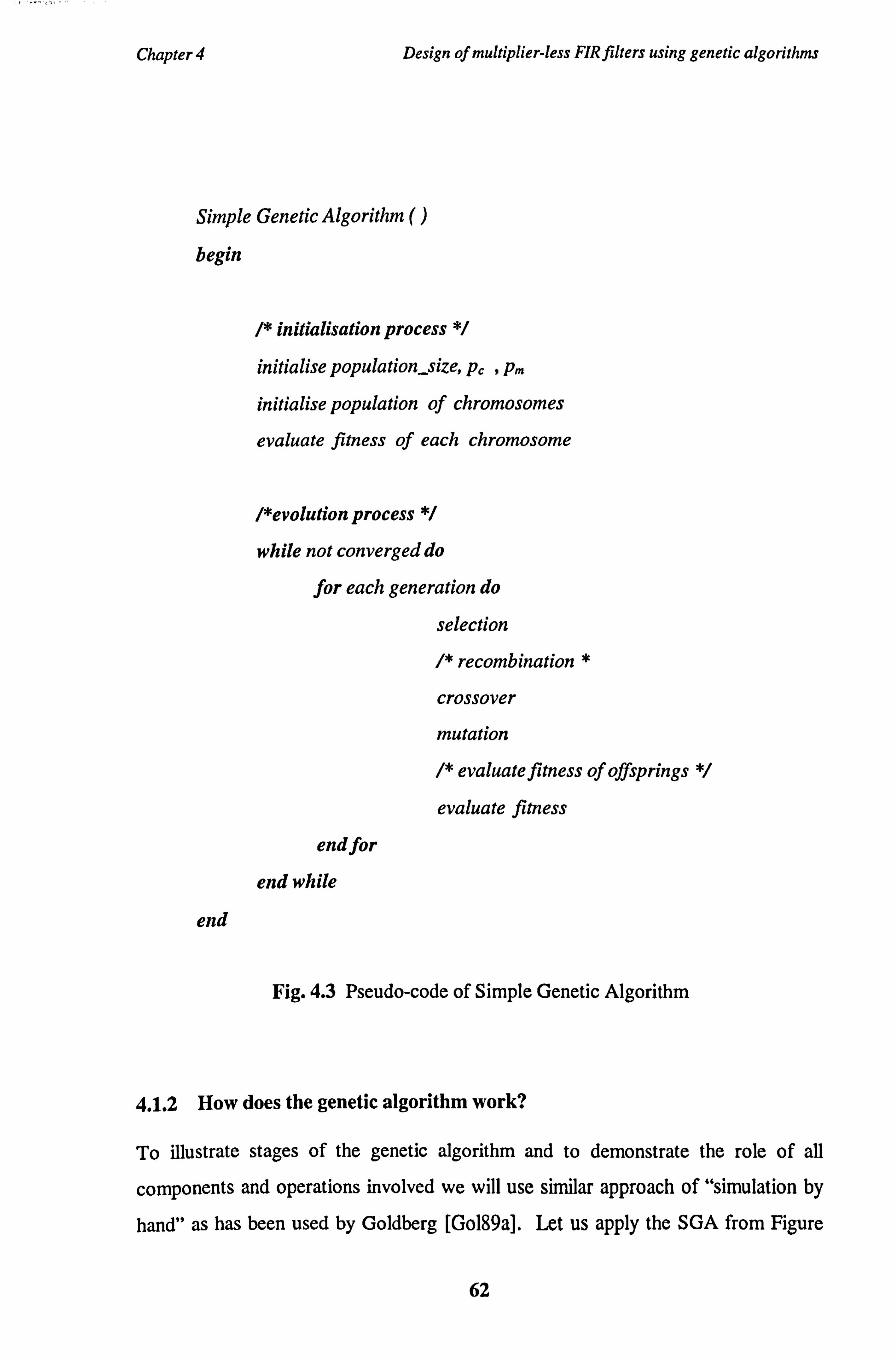
Chapter 4 Design of multiplier-less FIR filters using genetic algorithms
Simple Genetic Algorithm ()
begin
/* initialisation process */
initialise population-size, p, , pm
initialise population of chromosomes
evaluate fitness of each chromosome
/*evolution process */
while not converged do
for each generation do
selection
/* recombination
crossover
mutation
/* evaluate fitness of offsprings
evaluate fitness
end for
end while
end
Fig. 4.3 Pseudo-code of Simple Genetic Algorithm
4.1.2 How does the genetic algorithm work?
To illustrate stages of the genetic algorithm and to demonstrate the role of all
components and operations involved we will use similar approach of "simulation by
hand" as has been used by Goldberg [Go189a]. Let us apply the SGA from Figure
62
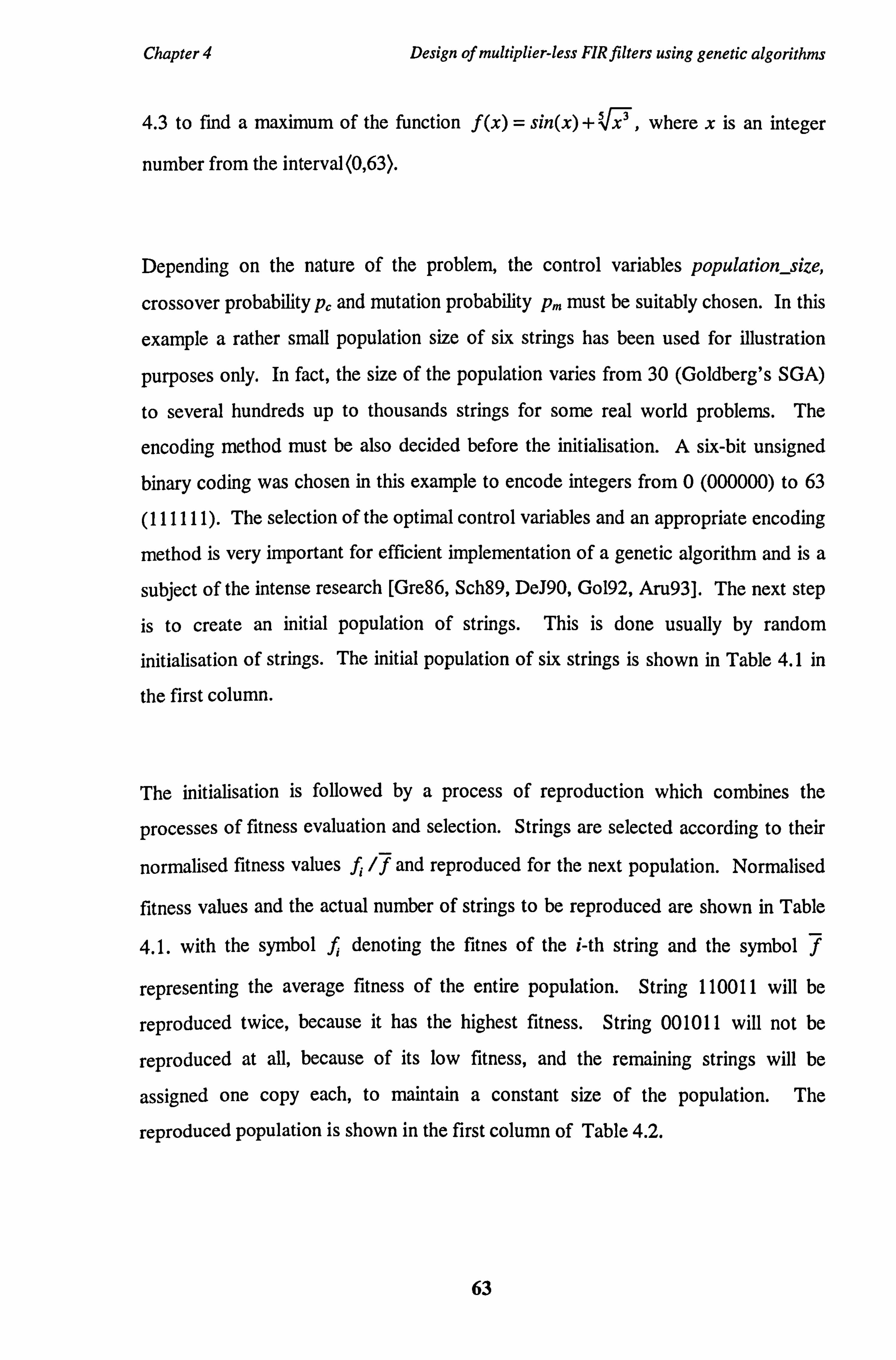
Chapter 4 Design of multiplier-less FIR filters using genetic algorithms
4.3 to find a maximum of the function f (x) = sin(x) +V x' , where x is an integer
number from the interval (0,63).
Depending on the nature of the problem, the control variables population_size,
crossover probability p, and mutation probability p�, must be suitably chosen. In this
example a rather small population size of six strings has been used for illustration
purposes only. In fact, the size of the population varies from 30 (Goldberg's SGA)
to several hundreds up to thousands strings for some real world problems. The
encoding method must be also decided before the initialisation. A six-bit unsigned
binary coding was chosen in this example to encode integers from 0 (000000) to 63
(111111). The selection of the optimal control variables and an appropriate encoding
method is very important for efficient implementation of a genetic algorithm and is a
subject of the intense research [Gre86, Sch89, DeJ90, Go192, Aru93]. The next step
is to create an initial population of strings. This is done usually by random
initialisation of strings. The initial population of six strings is shown in Table 4.1 in
the first column.
The initialisation is followed by a process of reproduction which combines the
processes of fitness evaluation and selection. Strings are selected according to their
normalised fitness values f,. /7 and reproduced for the next population. Normalised
fitness values and the actual number of strings to be reproduced are shown in Table
4.1. with the symbol f,. denoting the fitnes of the i-th string and the symbol 7
representing the average fitness of the entire population. String 110011 will be
reproduced twice, because it has the highest fitness. String 001011 will not be
reproduced at all, because of its low fitness, and the remaining strings will be
assigned one copy each, to maintain a constant size of the population. The
reproduced population is shown in the first column of Table 4.2.
63
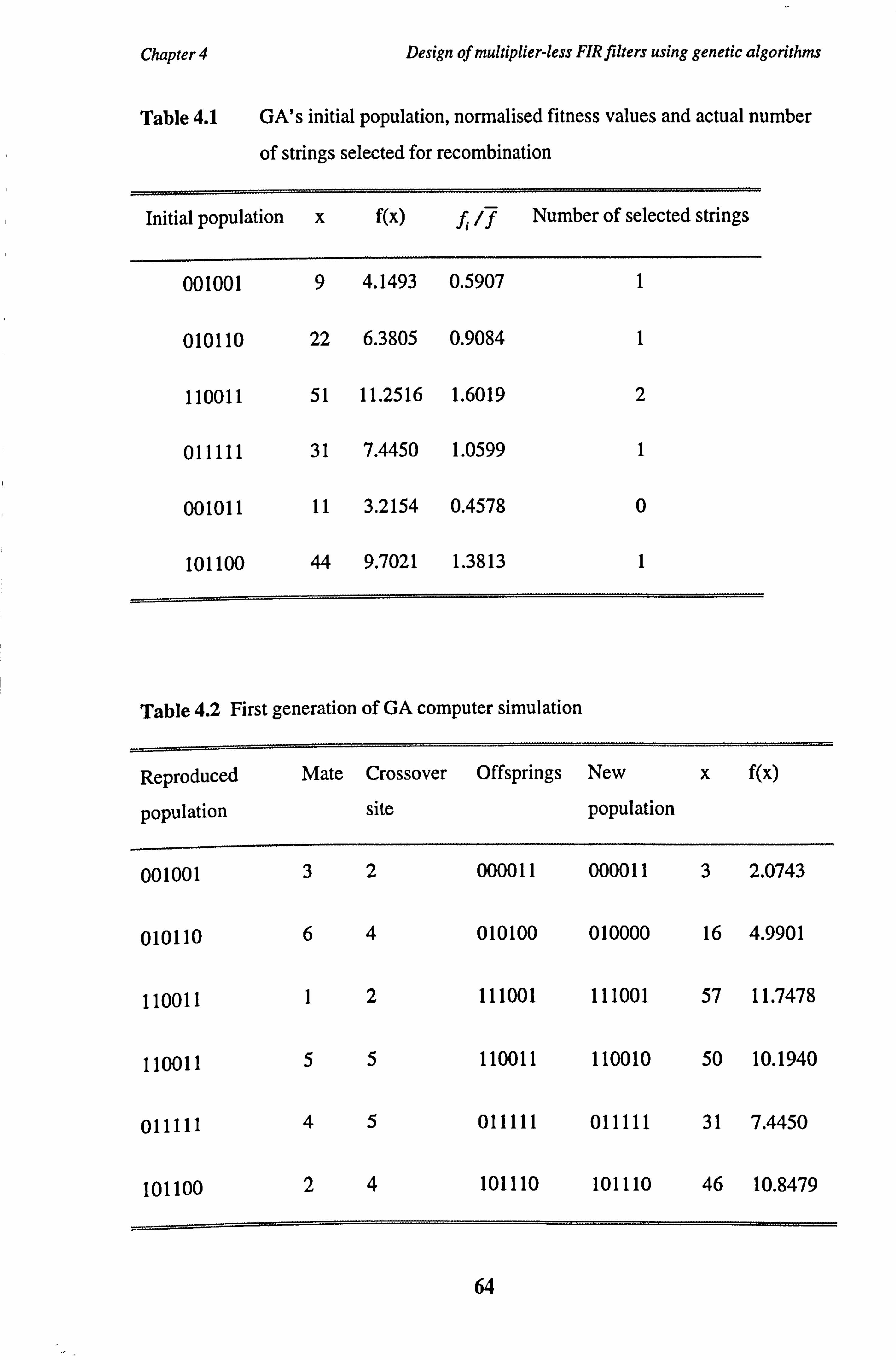
Chapter 4 Design of multiplier-less FIR filters using genetic algorithms
Table 4.1 GA's initial population, normalised fitness values and actual number
of strings selected for recombination
Initial population x f(x) f. /7 Number of selected strings
001001 9 4.1493 0.5907 1
010110 22 6.3805 0.9084 1
110011 51 11.2516 1.6019 2
011111 31 7.4450 1.0599 1
001011 11 3.2154 0.4578 0
101100 44 9.7021 1.3813 1
Table 4.2 First generation of GA computer simulation
Reproduced
population
Mate Crossover
site
Offsprings New
population
x f(x)
001001 3 2 000011 000011 3 2.0743
010110 6 4 010100 010000 16 4.9901
110011 1 2 111001 111001 57 11.7478
110011 5 5 110011 110010 50 10.1940
011111 4 5 011111 011111 31 7.4450
101100 2 4 101110 101110 46 10.8479
64

Chapter 4 Design of multiplier-less FIR filters using genetic algorithms
Following the process of reproduction, the crossover operator is applied in two steps.
In the first step, strings are randomly mated, using coin tosses to pair mates. In this
example, the first string was paired with the third, the second with the sixth and
fourth with fifth string. In the second step, a biased coin toss will decide if the
crossover will occur. If the result is heads, the strings swap their parts before and
after a randomly chosen crossover site (shown in the third column of Table 4.2), thus
generating offsprings. If the result is tails, the offsprings are the exact copies of
parent strings. After crossover, the mutation operator is applied, mutating randomly
string's bits with the probability pm. String 010100 was mutated at the fourth locus
(position) creating thus the string 010000 and string 110011 was mutated at the sixth
locus, creating the string 110010. Mutated strings are shown as the new population
in fifth column of Table 4.2. In this example, the SGA after first generation
produced a string 111001 which when decoded, returns higher value of the function
to be maximised, than the best string from the initial population (the string, its
decoded value and the function value is shown in italics in Table 4.2). Subsequent
generations would produce "better" strings, eventually a global maxima of the
function is attained. The algorithm terminates, when the total number of generations
has exceeded a specified amount or when the population has converged. The
population is converged, when all of the genes have converged. A gene is said to be
converged, when 95% of the population have identical value [DeJ75]. But why is the
Genetic Algorithm able to produce better strings by just selecting, copying and
crossing strings together?
The first explanations how GAs work was given by Holland's schema theorem
[Ho175]. A schema is a pattern of gene values describing a subset of chromosomes
which have similarities at certain positions. A chromosome contains a particular
schema if it matches that schema. For example, when using a binary coding with the
three symbols 1,0 and * (the symbol * can represent either 1 or 0), the string 111001
from the previous example contains schemata 11****, 11*0*1, **1001, etc.
Goldberg [Go189a] introduces the following two properties for schemata: defining
length and order. The defining length 8 of a schema H is the distance between the
65

Chapter 4 Design of multiplier-less FIR filters using genetic algorithms
outermost chromosome's position that are fixed (in this example, 8=1,5, and 3,
respectively). The order of a schema, denoted in GA literature as o(H), is the total
number of fixed positions. Schema theorem states:
Schema theorem.
The optimum way to explore a searching space is to allocate chances to individuals
to reproduce proportionally to their fitness relative to the average fitness of the
population. Good schemata are then exponentially increasing in numbers in
successive generations.
Holland also showed that the number of schemata processed in each generation is of
the order N pop 9 where Npop is the size of the population. This is very important and
powerful feature of genetic algorithms known as implicit parallelism.
The proof of the schema theorem and a theoretical analysis of the effect of
reproduction, crossover and mutation on a particular schema H was shown by
Goldberg in [Go189a]. We will repeat the proof here as it is a foundation for
understanding how genetic algorithms work. Let's suppose that in the discrete time
step t there are m examples of a schema H in a current population. We will denote
this as m= m(H, t), meaning that there are different numbers of different schemata H
at different times t. Each discrete time step represents one generation. An expected
number of schemataH in the next generation is therefore denoted as m= m(H, t+ 1).
The first step is to determine the effect of reproduction. Let's suppose that a
population contains n strings and the average fitness of all strings representing
schema H at time t isf(H). The expected number of schemata H at time t+1 is then
given by the following equation:
66

Chapter 4 Design of multiplier-less FIR filters using genetic algorithms
m(H, t+1)=m(H, t)"n"f(H) (4.1)
1f
As the average fitness of the population was defined as f=. f/n, equation (4.1) can
be rewritten as
m(H, t+ l) = m(H, t) f f) (4.2)
Equation (4.2) states that, during reproduction, schemata with fitness values above
the population average will receive increased number of copies for the next
generation and schemata with low fitness values will decrease in numbers (and
gradually will die off). To complete the proof of the schema theorem Goldberg has
also shown in [Gol89a] that good schemata are increasing in their numbers
exponentially.
Suppose that a schema H has an above average fitness f(H) =7+ C" f, where C is a
constant. Equation (4.2) after substituting f(H) and assuming a stationary value of C
becomes:
m(H, t+1)=m(H, t)`J +CfJ=(1+C)"m(H,
t) (4.3) f
and this can be rewritten as:
m(H, t+ 1) = m(H, O) " (1 + C)` (4.4)
This equation is also known as a discrete form of an exponential function. Hence, we have a proof that good schemata during reproduction are increasing in numbers
exponentially.
67

Chapter 4 Design of multiplier-less FIR filters using genetic algorithms
To analyse the effect of crossover, suppose a binary string of length L that contains a
particular schema H with defining length S(H). Schema H will be destroyed
(disrupted) by crossover, whenever a crossover point falls between any two bits
corresponding to schema H. Generally, the probability that a schema H will be
destroyed is:
Pd = PC L- (4.5)
where p, is the probability of crossover. The probability that a schema H will survive
crossover is defined as the mutation survival probabilityps,
psc z 1- pd =1- pc " L5(H) l (4.6)
Because the crossover operation is independent of the reproduction and follows the
reproduction stage, equation (4.2) can be multiplied by the survival probability psc to
obtain a combined effect of reproduction and crossover:
m(H, t+ 1) >_ m(H, t)- f (H) 1I-P,. L(Hi
(4.7)
The last step is to determine the effect of mutation. Mutation randomly alters each
allele of the string with the probability p, �. If a schema H has the o(H) fixed alleles,
each allele has to survive in order for a schema H to survive. The probability that an
allele survives mutation is (1 - p). Because there is no correlation between
mutations, the probability that a particular schema H with the o(H) fixed alleles
survives mutation is:
Pam = (1
- P. )o(H) (4.8)
68
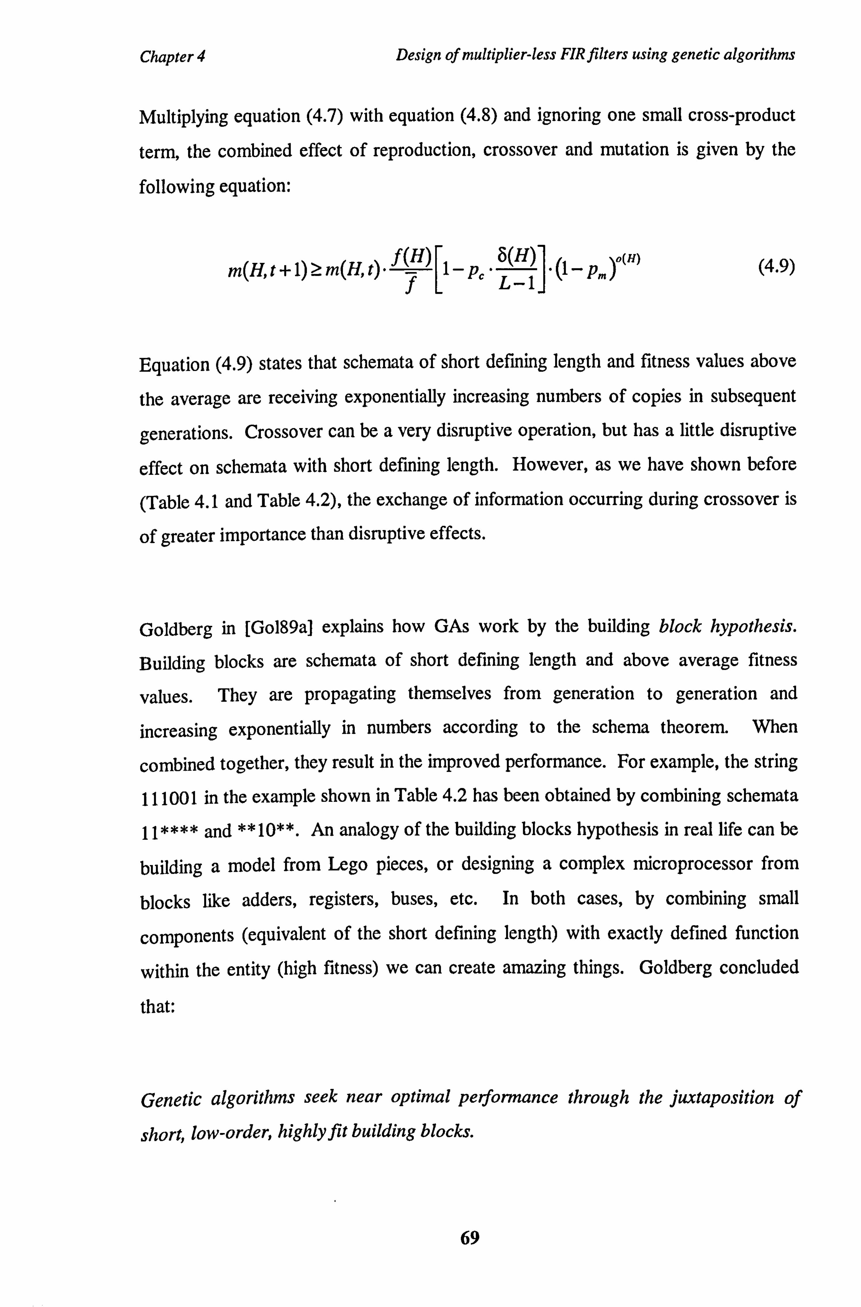
Chapter 4 Design of multiplier-less FIR filters using genetic algorithms
Multiplying equation (4.7) with equation (4.8) and ignoring one small cross-product
term, the combined effect of reproduction, crossover and mutation is given by the
following equation:
m(H, t+ 1) >- m(H, t) f (H)
1- pý " 8(H)
" ](1_Pm)(H)(4.9)
Equation (4.9) states that schemata of short defining length and fitness values above
the average are receiving exponentially increasing numbers of copies in subsequent
generations. Crossover can be a very disruptive operation, but has a little disruptive
effect on schemata with short defining length. However, as we have shown before
(Table 4.1 and Table 4.2), the exchange of information occurring during crossover is
of greater importance than disruptive effects.
Goldberg in [Gol89a] explains how GAs work by the building block hypothesis.
Building blocks are schemata of short defining length and above average fitness
values. They are propagating themselves from generation to generation and
increasing exponentially in numbers according to the schema theorem. When
combined together, they result in the improved performance. For example, the string
111001 in the example shown in Table 4.2 has been obtained by combining schemata
11**** and **10**. An analogy of the building blocks hypothesis in real life can be
building a model from Lego pieces, or designing a complex microprocessor from
blocks like adders, registers, buses, etc. In both cases, by combining small
components (equivalent of the short defining length) with exactly defined function
within the entity (high fitness) we can create amazing things. Goldberg concluded
that:
Genetic algorithms seek near optimal performance through the juxtaposition of
short, low-order, highly fit building blocks.
69
Chapter 4 Design of multiplier-less FIR filters using genetic algorithms
The formation of building blocks can be encouraged by a suitable coding method. A
good coding method will encode genes that are related to each other so that they will
appear close on the chromosome and the interaction between them will be as low as
possible. The crossover and mutation operations should also support a formation of
building blocks, with a minimum disruption. We will follow these principles in our
implementation of a simple genetic algorithm that is presented next.
4.2 Simple genetic algorithm for the FIR filter design
A mapping of the discrete combinatorial optimisation problem onto a genetic
algorithm is not a straightforward task. A thorough analysis of the optimisation
problem has to precede the mapping of the problem onto a genetic algorithm. When
this is omitted, the performance of genetic search is low and the results are more-less
random. This is in agreement with previous claims that genetic algorithms can find a
solution without any knowledge about the problem. This is true, yet the genetic
algorithm must:
perform the searching process in a domain where the problem is defined,
" know whether chromosomes represent good or poor potential solutions to the
problem.
The first requirement can be satisfied by a choice of an appropriate encoding scheme
and the second requirement is accomplished by constructing of a specific problem-
related fitness function.
The process of mapping the filter design problem onto the genetic algorithm is shown
next. The filter coefficients are encoded onto a population of chromosomes as they
are the parameters that need to be designed. The chromosomes can have any data
structure, in case of the simple genetic algorithm they are just binary strings. The
filter coefficients are evolved by the genetic manipulating of chromosomes.
70
Chapter 4 Design of multiplier-less FIR filters using genetic algorithms
When designing digital FIR filters the following considerations must be known:
" the desired frequency response, i. e. magnitude and phase response
" the filter order (N-1)
" coefficient wordlength
In case of multiplier-less FIR digital filters, additional restrictions on the range of
coefficient values must be also taken into account. These considerations greatly
influence the chromosome structure and the associated encoding method and also the
fitness function. The chromosome structure and the fitness function vary for each
particular filter.
The algorithm proposed here (further referred as GA-1) employs the SGA model and
can design linear-phase ML FIR filters of the following types: low-pass, high-pass,
band-pass, band-stop, multiple-band filters or filters with an arbitrary frequency
response. No other magnitude or phase constraints can be realised with the GA-1
algorithm. The filter coefficients are restricted to the PWR2 or 2PWR2. The source
code of GA-1 algorithm written in Matlab is included on the accompanying disk.
4.2.1 Encoding
In living organisms, the DNA carries an important genetic information of organisms
by the information onto the chromosomes. Genetic algorithms must have also a
similar system to encode parameters of the problem to be solved. Each individual
parameter (representing an individual gene) is encoded and genes are concatenated to
form chromosomes (strings of values). Encoding of the problem's parameters must
be decided before genetic algorithm can be considered to solve any problem. A
particular method of encoding depends on the nature of the problem and is very
critical to the performance of genetic algorithms.
71
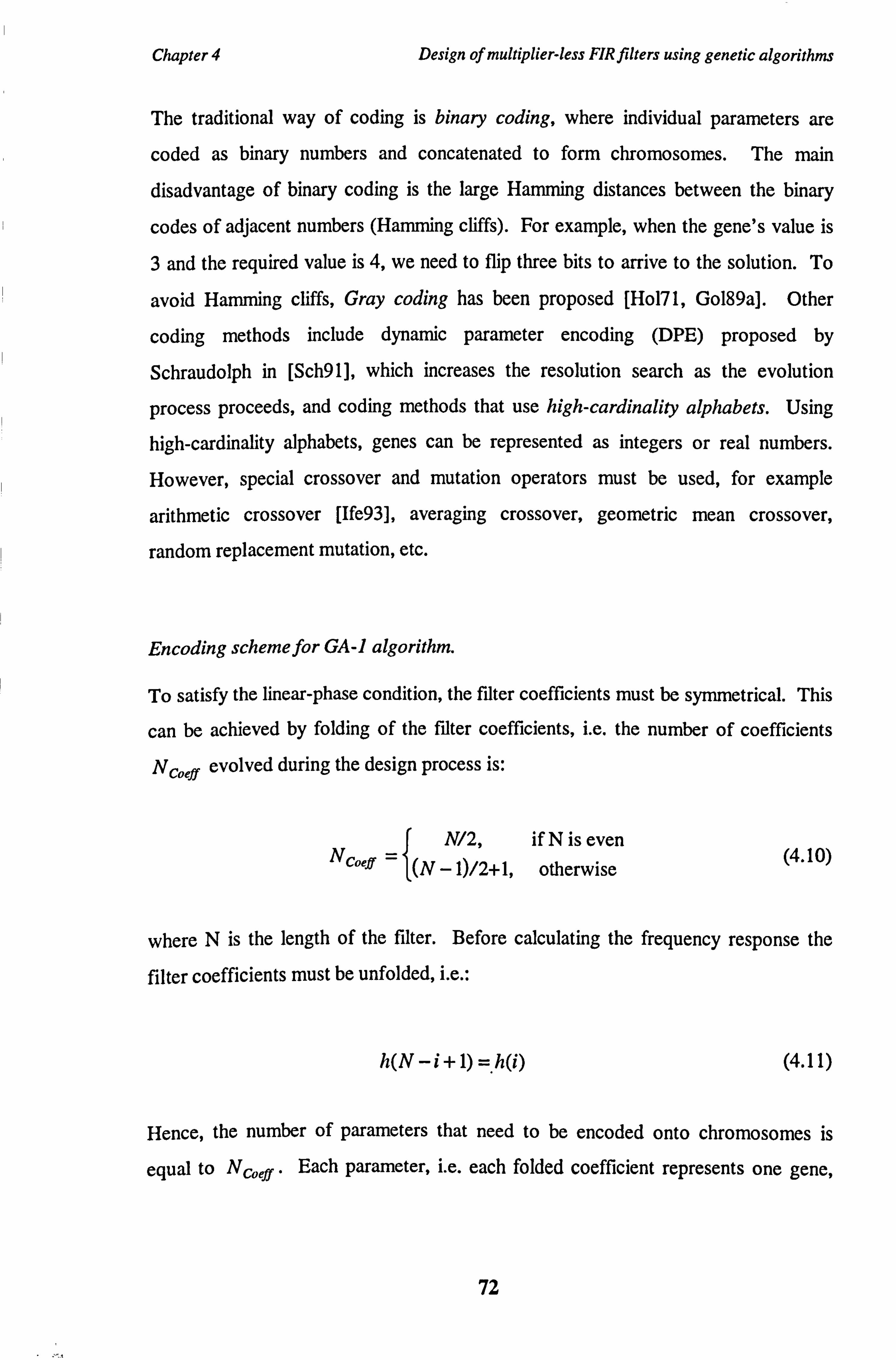
Chapter 4 Design of multiplier-less FIR filters using genetic algorithms
The traditional way of coding is binary coding, where individual parameters are
coded as binary numbers and concatenated to form chromosomes. The main
disadvantage of binary coding is the large Hamming distances between the binary
codes of adjacent numbers (Hamming cliffs). For example, when the gene's value is
3 and the required value is 4, we need to flip three bits to arrive to the solution. To
avoid Hamming cliffs, Gray coding has been proposed [Ho171, Go189a]. Other
coding methods include dynamic parameter encoding (DPE) proposed by
Schraudolph in [Sch9l], which increases the resolution search as the evolution
process proceeds, and coding methods that use high-cardinality alphabets. Using
high-cardinality alphabets, genes can be represented as integers or real numbers.
However, special crossover and mutation operators must be used, for example
arithmetic crossover [Ife93], averaging crossover, geometric mean crossover,
random replacement mutation, etc.
Encoding scheme for GA-1 algorithm.
To satisfy the linear-phase condition, the filter coefficients must be symmetrical. This
can be achieved by folding of the filter coefficients, i. e. the number of coefficients
NCOef evolved during the design process is:
N/2, if N is even NcOe (N -1)/2+1, otherwise
(4.10)
where N is the length of the filter. Before calculating the frequency response the
filter coefficients must be unfolded, i. e.:
h(N-i+1)=h(i) (4.11)
Hence, the number of parameters that need to be encoded onto chromosomes is
equal to Nook . Each parameter, i. e. each folded coefficient represents one gene,
72

Chapter 4 Design of multiplier-less FIR filters using genetic algorithms
therefore the chromosomes will have NCoeff genes in total. The values of the filter
coefficients h; (alleles) are assumed to be either single power-of-two values (PWR2):
h; E {a: a= c; " 2-b' , c; E {-1,1}, b, E {1,2, ..., B -1}} (4.12)
or the sum (or the difference) of two power-of-two values (2PWR2):
2
h; ýdi-2 -bý�d ; E{-1,0,1}, b; E{1,..., B-1} (4.13)
where B is the coefficient wordlength. For example, when the coefficient wordlength
B= 16, the filter coefficients can be any of the following values:
a) PWR2 12-i
_2-2 ..., -2-15, +2 -u +2-2 +2-11 (4.14)
b) 2PWR2
2-1-2-1, -2-1-2'2,..., -2-1s, (4.15) +2-'s,..., +2-1 +2-2, +2-1 +2-1
When designing ML FIR filters, the choice of filter coefficients is limited to discrete
values with highly non-uniform distribution. The distribution of PWR2 coefficients
in the interval (- 05, +05) is shown in Figure 4.4.
73
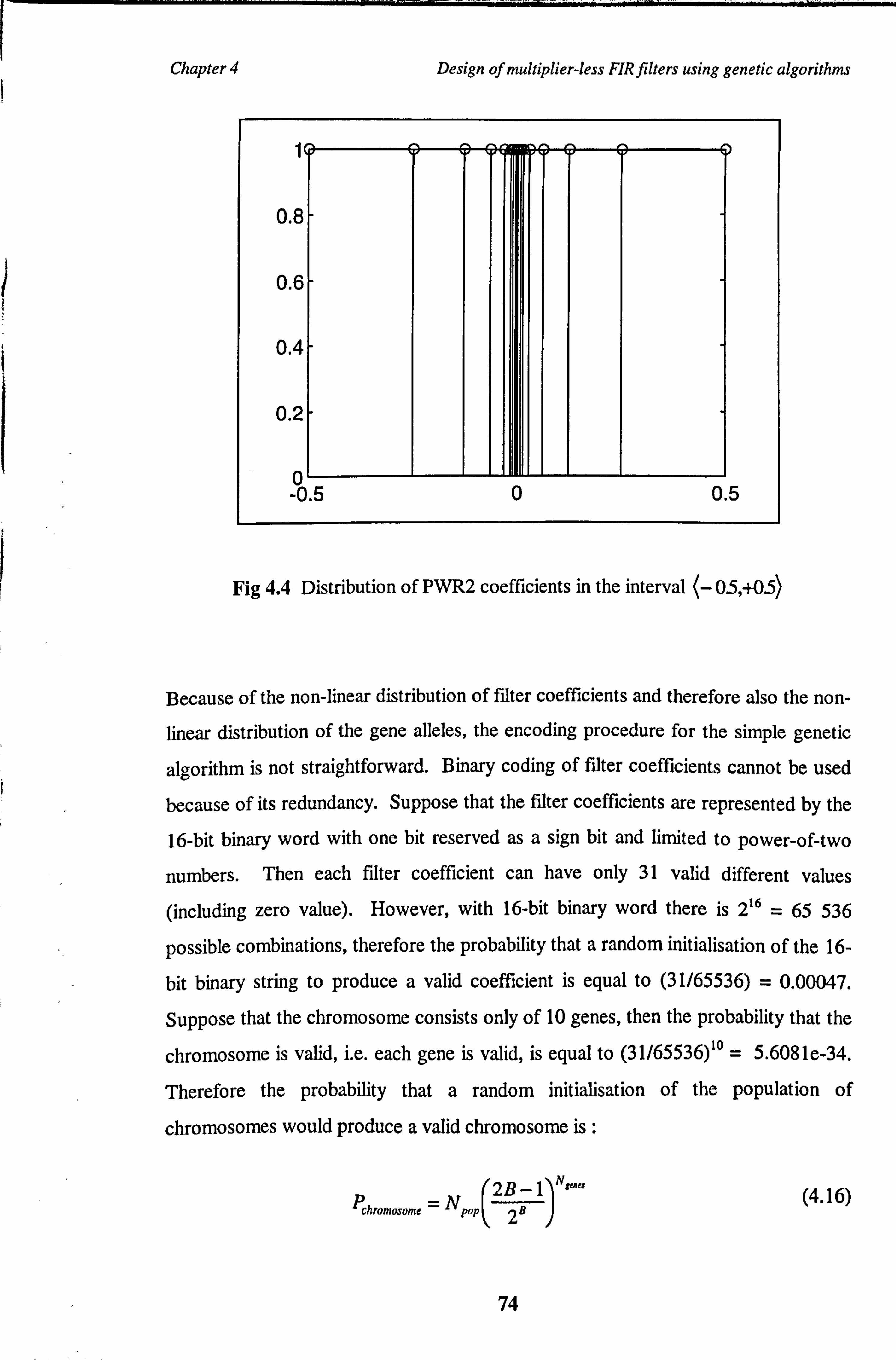
Chapter 4 Design of multiplier-less FIR filters using genetic algorithms
0.8-
0.6-
0.4-
0.2-
0 -0.5 0 0.5
Fig 4.4 Distribution of PWR2 coefficients in the interval (- 05, +05
Because of the non-linear distribution of filter coefficients and therefore also the non-
linear distribution of the gene alleles, the encoding procedure for the simple genetic
algorithm is not straightforward. Binary coding of filter coefficients cannot be used
because of its redundancy. Suppose that the filter coefficients are represented by the
16-bit binary word with one bit reserved as a sign bit and limited to power-of-two
numbers. Then each filter coefficient can have only 31 valid different values
(including zero value). However, with 16-bit binary word there is 216 = 65 536
possible combinations, therefore the probability that a random initialisation of the 16-
bit binary string to produce a valid coefficient is equal to (31/65536) = 0.00047.
Suppose that the chromosome consists only of 10 genes, then the probability that the
chromosome is valid, i. e. each gene is valid, is equal to (31/65536)10 = 5.6081e-34.
Therefore the probability that a random initialisation of the population of
chromosomes would produce a valid chromosome is :
2B -1 "sexes (4.16) Pchromosomc =N pop 2B
74

Chapter 4 Design of multiplier-less FIR filters using genetic algorithms
where Np0 is the size of the population (number of chromosomes) and Ngene, is the
number of genes in each chromosome:
Ngenes - Ncoeff
, 2- Ncoeff
for PWR2 coefficients for 2PWR2 coefficients
(4.17)
This redundancy produces a number of invalid strings that need to be removed from
the population in each generation. As a consequence, the performance of genetic
algorithm radically deteriorates.
Because of the redundancy problems we propose a different coding method. It follows
from the analysis of (4.14) and (4.15) that only the exponents of power-of-two
coefficients and the signs of coefficients need to be encoded. The exponent signs can be
ignored as they are always minus. As only 30 different coefficients are to be encoded
(when B= 16), only 5-bit binary word is needed where one bit is reserved for the sign.
The chromosome length Lchrom is a product of the number of genes Ngenes and the
number of bits Bgene required to encode each allele:
Lchrom = Ngenes * Bgene (4.18)
The encoding method is demonstrated by the following example.
Example:
We will demonstrate the encoding procedure using a 10-th order FIR filter with PWR2
coefficients and the coefficient wordlength B equal to 16, thus restricting the coefficient
values to be power-of-two values in the range (-2 -15 +2-15). A set of the filter
coefficients can have, for example, the following values:
h= {2-s, 2-a'2-15 2-2'2-15,2-1 , 2_15 2-2 , 2-15X2-4,2-s } (4.19)
75
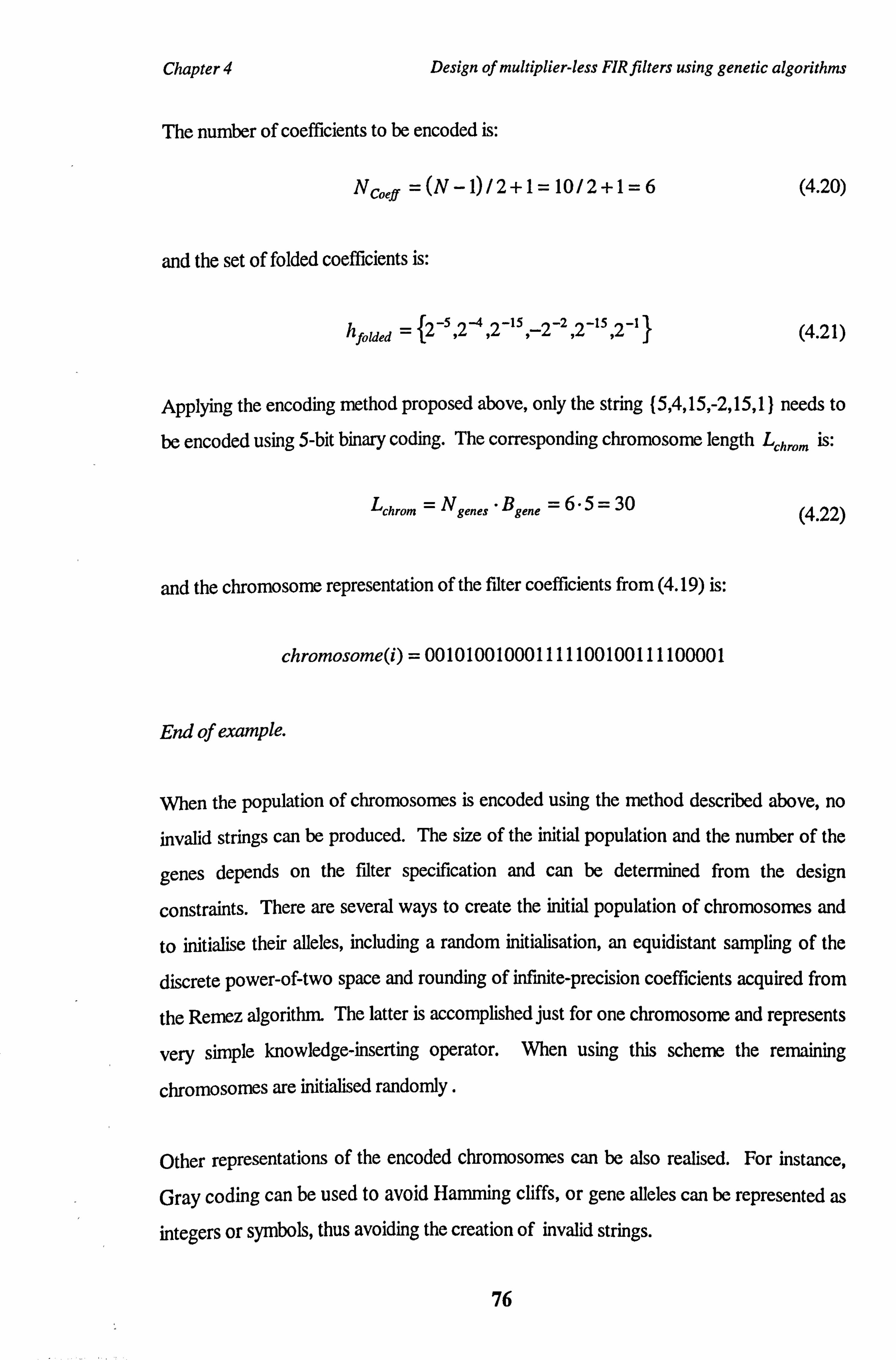
Chapter 4 Design of multiplier-less FIR filters using genetic algorithms
The number of coefficients to be encoded is:
NCoeff =(N-1)12+1=10/2-x-1=6 (4.20)
and the set of folded coefficients is:
hfolded = 12-5,2 -4
ý2-15 2-z
ý2-15 ý2-11 (4.21)
Applying the encoding method proposed above, only the string (5,4,15, -2,15,1 } needs to
be encoded using 5-bit binary coding. The corresponding chromosome length Lchrom is:
Lchrom = Ngenes ' Bgene =6 .5= 30 (4.22)
and the chromosome representation of the filter coefficients from (4.19) is:
chromosome(i) = 001010010001111100100111100001
End of example.
When the population of chromosomes is encoded using the method described above, no
invalid strings can be produced. The size of the initial population and the number of the
genes depends on the filter specification and can be determined from the design
constraints. There are several ways to create the initial population of chromosomes and
to initialise their alleles, including a random initialisation, an equidistant sampling of the
discrete power-of-two space and rounding of infinite-precision coefficients acquired from
the Remez algorithm The latter is accomplished just for one chromosome and represents
very simple knowledge-inserting operator. When using this scheme the remaining
chromosomes are initialised randomly .
Other representations of the encoded chromosomes can be also realised. For instance,
Gray coding can be used to avoid Hamming cliffs, or gene alleles can be represented as
integers or symbols, thus avoiding the creation of invalid strings.
76

Chapter 4 Design of multiplier-less FIR filters using genetic algorithms
There is an ongoing discussion between GA researchers concerning which
representation of genes is better. Goldberg has shown in [Go189a, Go190] that the
representation of genes with the minimal binary alphabet is more natural to genetic
algorithms. Representation with the smallest alphabet allows better sampling of the
searching space. This is because genes' alleles that can be either 0 or 1 effectively cut
the searching space in half. Goldberg also investigated Gray coding and concluded
that although it can help to avoid Hamming cliffs, it introduces non-linearity in the
recombination process [Go189b]. Davis [Dav9l] argues in favour of nonbinary
higher cardinality alphabets as the larger range of operators can be applied to the
problem.
When using binary and Gray coding, crossover operator can have very disruptive
effects on the overall performance of the algorithm. This occurs when the crossover
point falls between any two bits of the gene that has converged to the genuine (and
correct) value. Therefore, we have implemented non disruptive crossover methods,
where the crossover point is guaranteed to be between outermost bits of the adjacent
genes. The influence of various gene representations on a performance of genetic
algorithm has been investigated, using the evolution speed as a criterion to measure
the effects of various gene representation. We have defined the evolution speed as
follows:
Definition 1.
Evolution speed is a number of generations that is necessary for genetic algorithm to
produce a chromosome that represents an acceptable solution to the problem being
solved.
Statistical analysis has shown that there is a little difference between results achieved
with various gene representations for ML FIR filter design problems. Therefore we
77
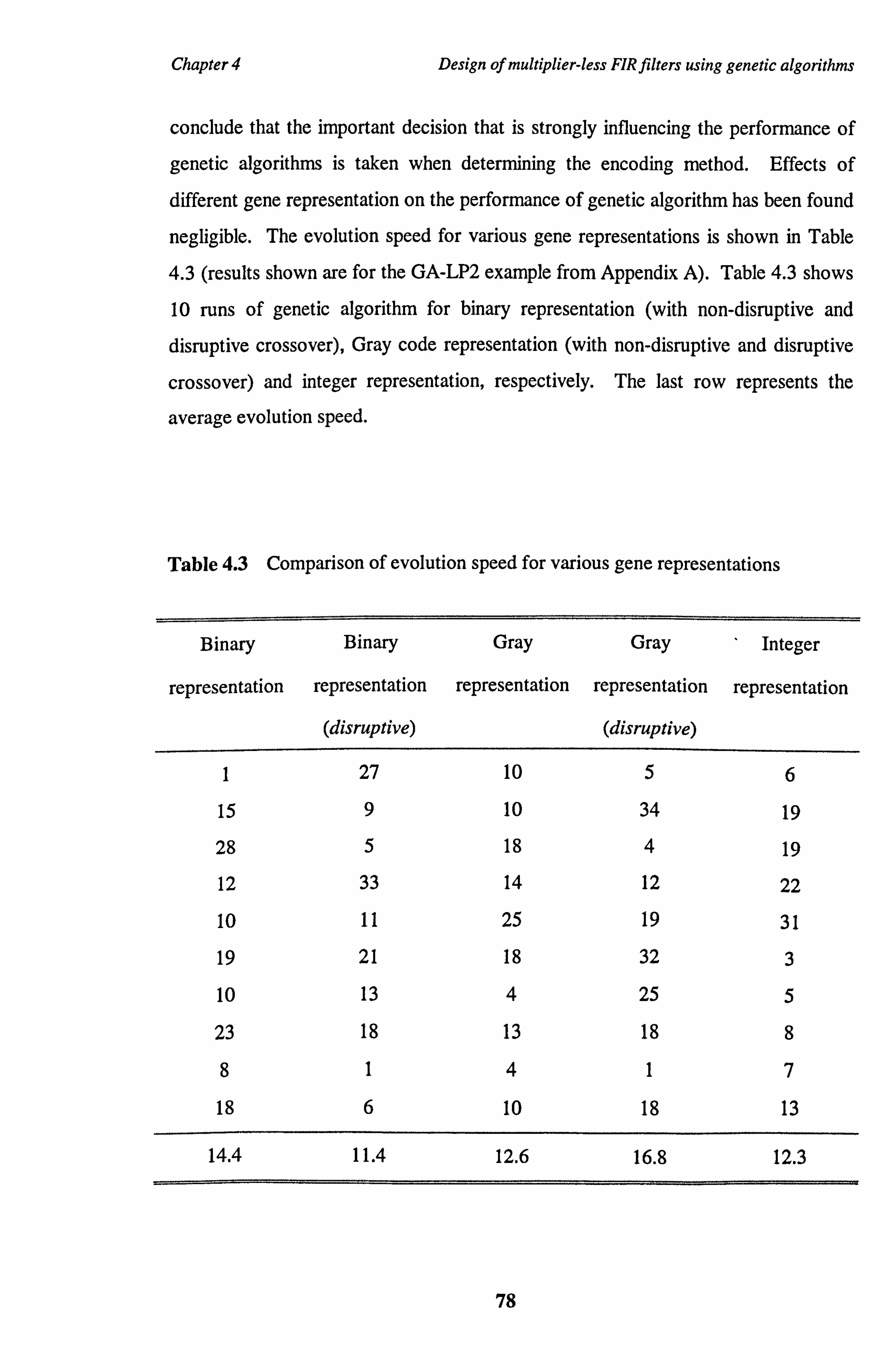
Chapter 4 Design of multiplier-less FIR filters using genetic algorithms
conclude that the important decision that is strongly influencing the performance of
genetic algorithms is taken when determining the encoding method. Effects of
different gene representation on the performance of genetic algorithm has been found
negligible. The evolution speed for various gene representations is shown in Table
4.3 (results shown are for the GA-LP2 example from Appendix A). Table 4.3 shows
10 runs of genetic algorithm for binary representation (with non-disruptive and
disruptive crossover), Gray code representation (with non-disruptive and disruptive
crossover) and integer representation, respectively. The last row represents the
average evolution speed.
Table 4.3 Comparison of evolution speed for various gene representations
Binary Binary Gray Gray Integer
representation representation representation representation representation
(disruptive) (disruptive)
1 27 10 5 6
15 9 10 34 19
28 5 18 4 19
12 33 14 12 22
10 11 25 19 31
19 21 18 32 3
10 13 4 25 5
23 18 13 18 8
8 1 4 1 7
18 6 10 18 13
14.4 11.4 12.6 16.8 12.3
78

Chapter 4 Design of multiplier-less FIR f lters using genetic algorithms
The decoding procedure is a reverse process of encoding. The chromosomes are
split into the genes that are decoded creating thus folded filter coefficients. The filter
coefficients are constructed by unfolding of the folded filter coefficients.
4.2.2 Fitness evaluation
The fitness function is the most important part of any genetic algorithm influencing its
overall performance. GA assigns a fitness value to each string, reflecting a potential
of the string to be a solution to the problem. To choose the fitness function is
straightforward in many cases. For instance, when maximising (minimising) function
f(x), where xE (x,, x2)1 the fitness value can be simply a value of the function at a
given point x (or a reciprocal function value). For complex design problems, when
many parameters are to be optimised, the fitness function should reflect all these
parameters. To construct a fitness function for multi-parameter optimisation
problems is non trivial task. When the values of decoded chromosomes have no
actual meaning for guiding a searching process, they cannot be used as a fitness
measure. Therefore, the fitness function that describes how well are chromosomes
progressing towards the local (global) optimum, must be constructed.
Fitness function for GA-1 algorithm.
The fitness function should express how accurately the desired frequency response is
approximated by the frequency response of the potential solution (decoded
chromosome) over the entire frequency range. The difference between both
frequency responses can be expressed as the weighted error function E(fi):
E(fi)= W(fi). [H(f, )_D(fi)] (4.23)
where H(f; ) is the actual frequency response of the FIR filter, D(ff) is the desired
frequency response and W(fj) is the weight function that controls the error ripples in
different bands (see also (2.13) in Chapter 2).
79

Chapter 4 Design of multiplier-less FIR filters using genetic algorithms
The FIR filter design problem can be then viewed as a minimisation of the error
function E(f j) over the frequency range fE (0, ir) for a given filter specification :
min 11 E(f, ) = W(fý) .[ H(f) - D(fi)] 11 (4.24) which must satisfy the filter specification
E(f; ) = W(fi) "[ H(f; ) - D(. f; )] Sf (4.25)
The fitness function should guarantee that the genetic algorithm will minimise an
error between the desired and actual frequency response, therefore it should be an
inverse function of the error function. The error function can be calculated as a mean
square error over the entire frequency range. Hence, the fitness function for the j-th
chromosome is given as follows:
fitness = 1
1+ [D(f) - Hi (f)]2 (4.26) Nf, f, =,
where Nfs represents the number of frequency samples. Within the process of fitness
evaluation, the frequency response is calculated and compared with the desired frequency
response at N fs discrete frequencies. The algorithm is terminated when the frequency
response is within the specification. Considering four basic types of FIR filters, the
fitness function (4.26) can be rewritten to reflect a specific frequency response of
each filter type:
80
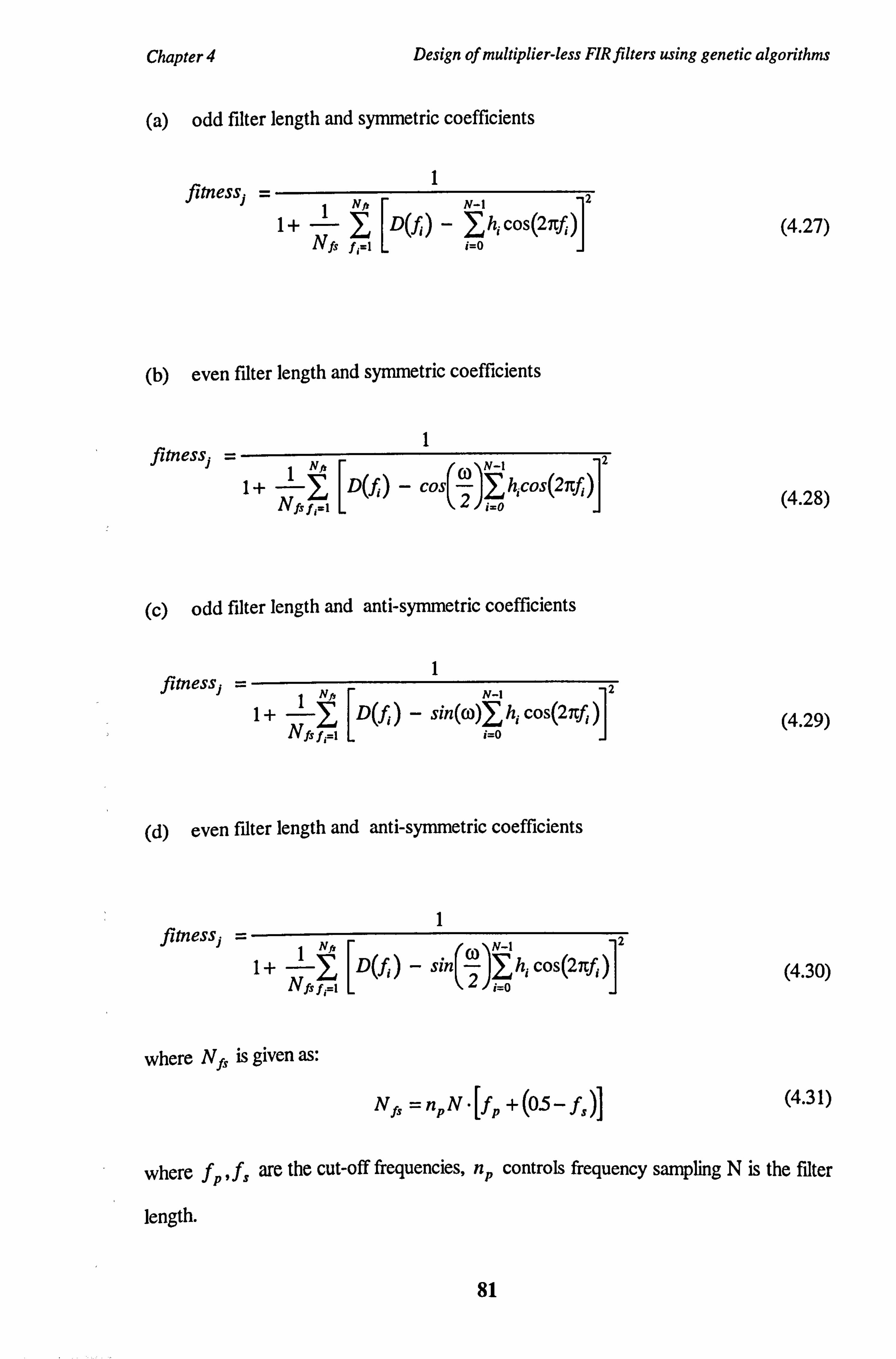
Chapter 4 Design of multiplier-less FIR filters using genetic algorithms
(a) odd filter length and symmetric coefficients
fitness -12 Nfi N-1
1+ 1 D(f) - lh; cos(21fi) (4.27) Nfs f, =i i=O
(b) even filter length and symmetric coefficients
i fitness = Nft N-t 2 1+1
[D(3) CO (4.28)
I- cos Ntst1
h cos(2) i=o
(c) odd filter length and anti-symmetric coefficients
1 fitness f2 Nf, N-1
1+1 D(f. ) - sin(co)1 h; cos(2nf) (4.29) Nfs fi ; _o
(d) even filter length and anti-symmetric coefficients
fitness] = 1
(l2 1+1 D(fi) - sing Jý hi cos(2nf
NfSf, =i \
i-o
where N f, is given as:
N fs = npN " [f
p +(05- fs)]
(4.30)
(4.31)
where fp, fs are the cut-off frequencies, np controls frequency sampling N is the filter
length.
81

Chapter 4 Design of multiplier-less FIR filters using genetic algorithms
4.2.3 Implementation of GA-1 algorithm.
It follows from the analysis of (4.27-4.30) that a design of digital FIR filters of (N-1)
order can be considered as N-dimensional combinatorial optimisation problem. The
algorithm proposed here uses Goldberg's Simple Genetic Algorithm (SGA) to search in
the discrete domain of powers-of-two for a combination of filter coefficients that best
satisfy the filter specification.
The GA-1 algorithm starts with a random population of chromosomes. The length and
the structure of chromosomes are determined by the filter length, filter type and the
applied encoding method. The default size of the population is 40 and can be changed by
the designer. Increasing of the size of the population Nn0 greatly influences searching
capabilities of the genetic algorithm, as the number of schemata processed in each
generation is of the order Np0 [Ho175]. Therefore a compromise between the size
of the population, the available computer memory and the convergence speed of
genetic algorithm has to be made.
In the next stage, the fitness values of chromosomes are evaluated. This is done in
two steps. First, chromosomes are decoded and unfolded, thus creating vectors of
filter coefficients. Then the frequency response of each coefficient vector is
calculated. The fitness values are determined according to the equations (4.27),
(4.28), (4.29) and (4.30).
Following the calculation of fitness values, offspring population is selected from the
parent population according to the fitness values of parent chromosomes. Fitness-
proportionate selection has been used in GA-1 algorithm. Half of the offspring
population represents father chromosomes, while the other half represents mother
chromosomes. Crossover sites are randomly choosen and the single point crossover
operator is applied to father and mother chromosome pairs with the probability P,,
thus creating a population of child chromosomes. The crossover probability P, 51,
82

Chapter 4 Design of multiplier-less FIR filters using genetic algorithms
hence allowing to keep some parent chromosomes in children population with no
changes. (default value of P, = 0.7). The process of crossover is followed by the
mutation. The probability of mutation P. is kept very low (default value of
Pm=0.001), otherwise genetic algorithms are reduced to a random search. During
the process of crossover and mutation, the parent population is replaced with the
population of offsprings.
Two generation replacement models have been tested with GA-1 algorithm. Initially,
a model using only one father chromosome has been used. We have denoted this
model as one father model. In one father model, the parent population is copied into
the offspring population and the chromosome with the highest fitness in the parent
population is selected as a father chromosome. This model preserves the best
chromosome in successive generations (population elitism), therefore it can be used
to refine the solution that has been found earlier or that has been found by other
algorithms. The father chromosome is crossed with other chromosomes in the parent
population (mothers) at every possible crossing point resulting in the creation of
offspring chromosomes. The frequency response of every offspring chromosome is
calculated, then compared with the desired frequency response and finally, the fitness
value is calculated. When the offspring chromosome has better fitness than the
chromosome with the worst fitness in the parent population, then it replaces the
worst chromosome. This process is repeated until all possible combinations of
[father I mother] crossing sites are exhausted. Following the process of selection
and crossover, the supervised mutation operator is applied. This is accomplished by
the inversion of every allele for each chromosome. A mutated chromosome is
inserted into the offspring population when its fitness is better than the fitness of the
worst chromosome. However, we have found that the one father model was very
slow and did not produce better results than the traditional generation-replacement
model.
83

Chapter 4 Design of multiplier-less FIR filters using genetic algorithms
The cycle of fitness evaluation, selection, crossover and mutation is repeated until no further improvements in the fitness function are achieved. If no solution is found, the
filter length is incremented and the GA-1 algorithm is repeated. Pseudo-code of the
proposed filter design algorithm is illustrated in Figure 4.5.
Genetic Filter Design ()
begin
*/filter specification */
specify the frequency response, filter type and coefficient type
while no acceptable solution was found do
create the initial population of chromosomes
evaluate fitness of chromosomes
while not converged do
for each generation do
select parent chromosomes for recombination
perform crossover
perform mutation
evaluate fitness of offspring chromosomes
/* generation replacement */
replace parent population with offsprings
end for
end while
/* increment the length of filter and run GA again */
if no acceptable solution was found
increment the length of f lter
end if
end while
end
Fig. 4.5 Pseudo-code of the GA-1 filter design algorithm
84
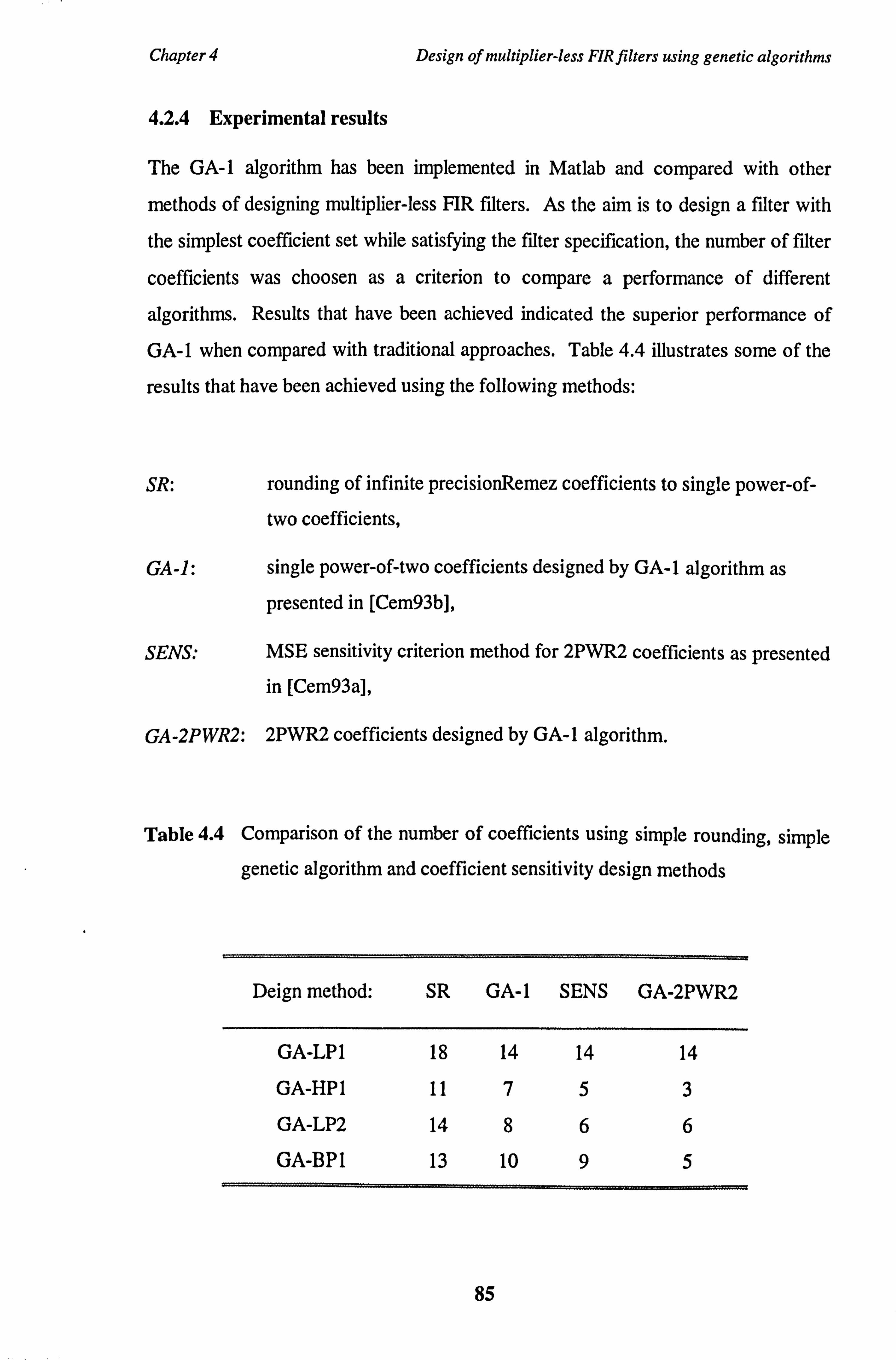
Chapter 4 Design of multiplier-less FIR filters using genetic algorithms
4.2.4 Experimental results
The GA-1 algorithm has been implemented in Matlab and compared with other
methods of designing multiplier-less FIR filters. As the aim is to design a filter with
the simplest coefficient set while satisfying the filter specification, the number of filter
coefficients was choosen as a criterion to compare a performance of different
algorithms. Results that have been achieved indicated the superior performance of
GA-1 when compared with traditional approaches. Table 4.4 illustrates some of the
results that have been achieved using the following methods:
SR: rounding of infinite precisionRemez coefficients to single power-of-
two coefficients,
GA-1: single power-of-two coefficients designed by GA-1 algorithm as
presented in [Cem93b],
SENS: MSE sensitivity criterion method for 2PWR2 coefficients as presented in [Cem93a],
GA-2PWR2: 2PWR2 coefficients designed by GA-1 algorithm.
Table 4.4 Comparison of the number of coefficients using simple rounding, simple
genetic algorithm and coefficient sensitivity design methods
Deign method: SR GA-1 SENS GA-2PWR2
GA-LP1 18 14 14 14
GA-HP I 11 753
GA-LP2 14 866
GA-BPI 13 10 95
85
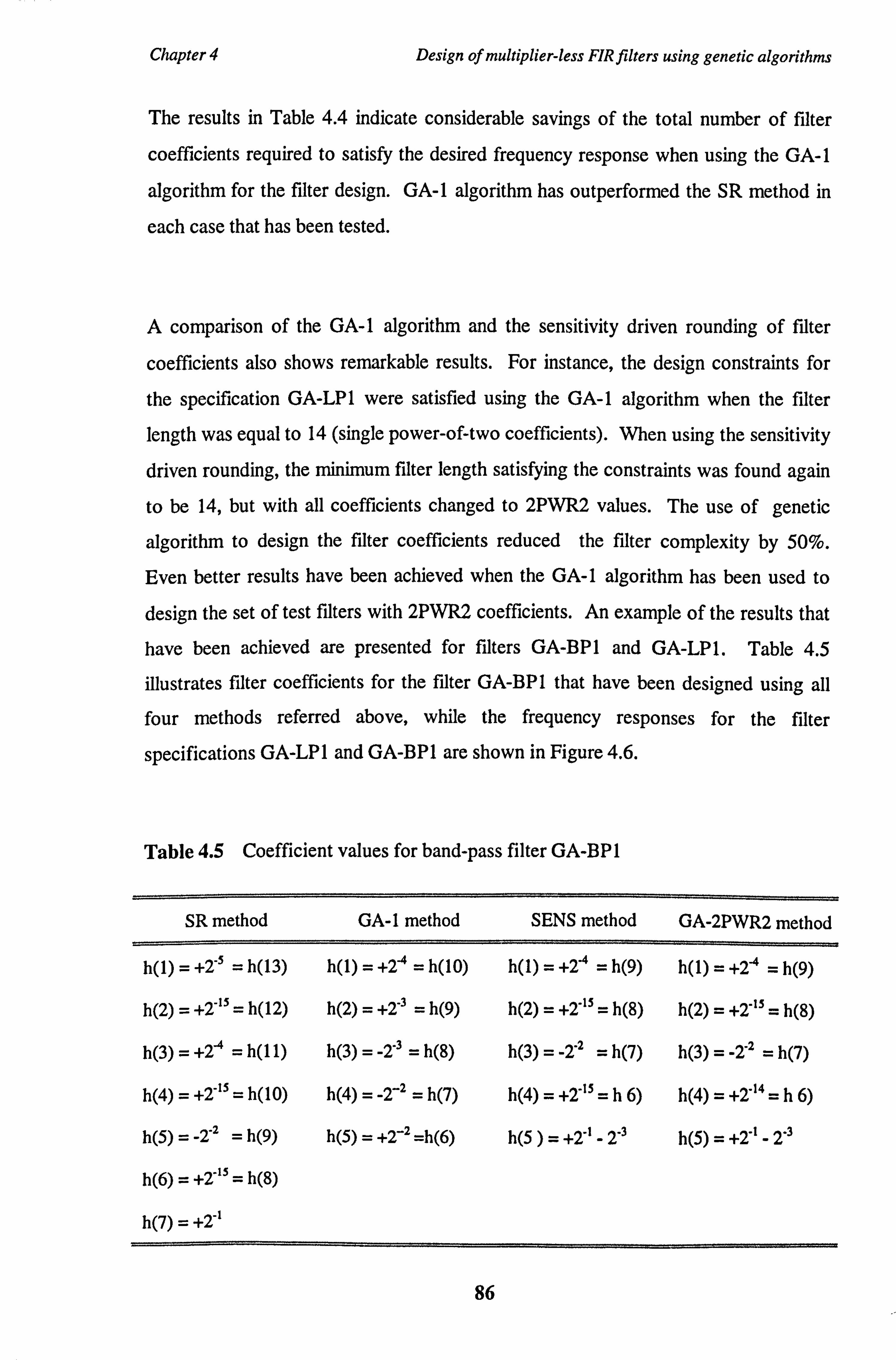
Chapter 4 Design of multiplier-less FIR filters using genetic algorithms
The results in Table 4.4 indicate considerable savings of the total number of filter
coefficients required to satisfy the desired frequency response when using the GA-1
algorithm for the filter design. GA-1 algorithm has outperformed the SR method in
each case that has been tested.
A comparison of the GA-1 algorithm and the sensitivity driven rounding of filter
coefficients also shows remarkable results. For instance, the design constraints for
the specification GA-LP1 were satisfied using the GA-1 algorithm when the filter
length was equal to 14 (single power-of-two coefficients). When using the sensitivity
driven rounding, the minimum filter length satisfying the constraints was found again
to be 14, but with all coefficients changed to 2PWR2 values. The use of genetic
algorithm to design the filter coefficients reduced the filter complexity by 50%.
Even better results have been achieved when the GA-1 algorithm has been used to
design the set of test filters with 2PWR2 coefficients. An example of the results that
have been achieved are presented for filters GA-BPI and GA-LP1. Table 4.5
illustrates filter coefficients for the filter GA-BP1 that have been designed using all
four methods referred above, while the frequency responses for the filter
specifications GA-LP1 and GA-BPI are shown in Figure 4.6.
Table 4.5 Coefficient values for band-pass filter GA-BPI
SR method GA-1 method SENS method GA-2PWR2 method
h(1) = +2"5 = h(13) h(1) = +24 = h(10) h(1) = +2-4 = h(9) h(1) = +2-4 = h(9)
h(2) = +2"15 = h(12) h(2) = +2-3 = h(9)
h(3) = +274 = h(11) h(3) = -2'3 = h(8)
h(4) = +2-15 = h(10) h(4) = -2-2 = h(7)
h(5) = -2'2 = h(9) h(5) = +2_2 =h(6)
h(6) = +2-ß5 = h(8)
h(2) _ +2'15 = h(8) h(2) _ +2"15 = h(8)
h(3) _ -2'2 = h(7) h(3) _ -2'Z = h(7)
h(4)=+2'15 =h6) h(4)=+2'14=h6)
h(5 )= +2" -2 '3 h(5) _ +27' - 2'3
h(7) = +2 i
86

Chapter 4 Design of multiplier-less FIR filters using genetic algorithms
10
0
-10 -20
-so C ßö-40
-50
-60
-70
-Pn
SGA algorithm
_ SR algorithm
0 0.1 0.2 0.3 0.4 0.5 Normalised Frequency
(a)
1.2
.... SGA algorithm
1_ SR algorithm
0.8
«r- 0.6 C) 2
0.4
OL 0
0.2
0.1 0.2 0.3 0.4 Normalised Frequency
(b)
0.5
Fig. 4.6 Frequency responses for the GA-LP1 and GA-BPI filter specifications
87

Chapter 4 Design of multiplier-less FIR filters using genetic algorithms
4.3 Knowledge-based genetic algorithm
GA-1 algorithm based on SGA model that has been described in previous sections
does not require any prior information about the problem being solved. However, in
certain situations genetic algorithms can benefit from the additional knowledge that
would support the evolution process. Considering the design of multiplier-less FIR
filters, the knowledge can be inserted into the initial population in the form of
knowledge-based chromosome. This chromosome can be a coefficient vector that
has been designed using Remez algorithm or other suitable technique and rounded to
the nearest single power-of-two coefficients. The rationale behind this approach is to
refine the coefficient vectors that have been acquired by other techniques.
Coefficient vector that has been inserted into the initial population can be refined
during the evolution process, because genetic algorithm cannot converge to worse
chromosome (with lower fitness) as the knowledge-based chromosome. However,
the following requirements must be satisfied:
" genetic algorithm should propagate the best chromosome from population to
population,
" suitable mechanisms to avoid premature convergence must be implemented.
The first requirement can be implemented within the generation replacement process
that must guarantee that the best chromosome is copied from the parent population
into the offspring population without changes. The proportion of strings in the
population, which is replaced in each generation following the operation of selection,
reproduction and recombination, is defined as the generation gap. Traditionally,
researchers have used generation gap equal to 1 (Goldberg's Simple Genetic
Algorithm). It means, that the entire population is replaced in each population. This
method of replacement is often referred to as generational-replacement. It is not
suitable for our purpose, because there is no guarantee that the best chromosome will
be always propagated from generation to generation.
88

Chapter 4 Design of multiplier-less FIR filters using genetic algorithms
The other method, termed as steady-state replacement [Sys89, Whi89, Dav9l]
replaces only a part of the population, usually chromosomes with the lowest or below
the average fitness, while preserving the best chromosomes. Preservation of best
chromosomes for future generations is referred to as population elitism. The steady-
state replacement might be a better model of what is happening in nature, because it
allows coexistence of parents and offsprings. Goldberg and Deb examined [Go191 ]
both replacement methods and did not find any replacement method fundamentally
better than other. However, for our purpose the steady-state replacement model is
more suitable.
The problem of premature convergence is associated with the chromosomes with
high fitness values that are well above the average fitness value of the population.
These highly fit chromosomes can take over the entire population during the first few
generations, causing a convergence to a local maximum (minimum). To avoid the
premature convergence, various fitness re-mapping methods have been proposed,
including fitness scaling and fitness ranking [Go189a, Whi89]. Among several fitness
scaling and ranking methods, we have choosen linear scaling because of its simplicity.
Linear fitness scaling ensures that the maximum value of the scaled fitness is only 1.5
to 2.0 times higher than the average fitness of the population. In this way, the
maximum number of offsprings allocated to highly fit strings is two. The scaled
fitness values are calculated as follows:
fscaled = of +b
(4.32)
where a, b are constants which must be calculated in each generation. Constants a, b
must be chosen to prevent negative fitness values to be generated.
89

Chapter 4 Design of multiplier-less FIR filters using genetic algorithms
The pseudo-code of the knowledge-based genetic algorithm for the design of FIR
filters (further referred to as GA-2 algorithm) is shown in Figure 4.7. GA-2
algorithm has been tested on the set of filter specifications (Appendix A).
Knowledge-based chromosomes were represented as Remez coefficients rounded to
nearest single power-of-two terms. Results are shown in Table 4.6 (results shown
are for the GA-LP2 example). The improvement of evolution speed has been
achieved, when compared with Table 4.3 that shows results for the same experiment,
but without the knowledge chromosomes inserted into the initial population. The last
row represents the average evolution speed for various gene representation using
knowledge-based chromosomes.
Table 4.6 Comparison of evolution speed (knowledge-based genetic algorithm)
Binary Binary Gray Gray Integer
representation representation representation representation representation
(disruptive) (disruptive)
7 9 9 6 5
5 1 10 4 5
8 5 14 13 3
16 7 15 17 17
7 12 7 5 8
10 12 13 19 19
19 4 6 21 30
9 22 19 8 9
4 5 2 16 14
15 8 7 19 20
10.0 8.5 10.2 12.8 13.0
90
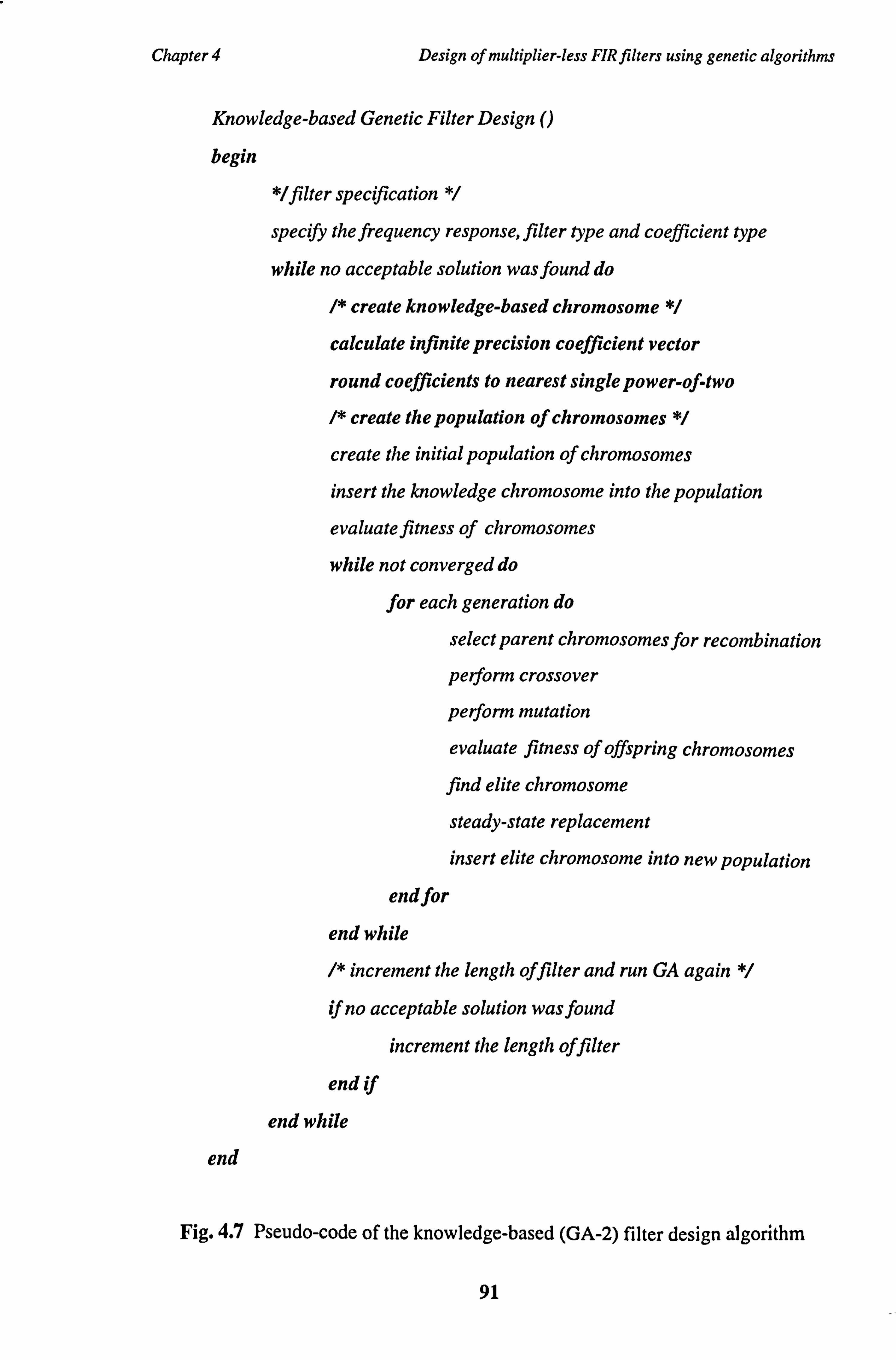
Chapter 4 Design of multiplier-less FIR filters using genetic algorithms
Knowledge-based Genetic Filter Design ()
begin
*/filter specification
specify the frequency response, filter type and coefficient type
while no acceptable solution was found do
/* create knowledge-based chromosome */
calculate infinite precision coefficient vector
round coefficients to nearest single power-of-two
/* create the population of chromosomes */
create the initial population of chromosomes
insert the knowledge chromosome into the population
evaluate f tness of chromosomes
while not converged do
for each generation do
select parent chromosomes for recombination
perform crossover
perform mutation
evaluate fitness of offspring chromosomes
find elite chromosome
steady-state replacement
insert elite chromosome into new population
end for
end while /* increment the length of filter and run GA again
if no acceptable solution was found
increment the length of filter
end if
end while
end
Fig. 4.7 Pseudo-code of the knowledge-based (GA-2) filter design algorithm
91

Chapter 4 Design of multiplier-less FIR filters using genetic algorithms
4.4 Hybrid GA-SA algorithm
In next section we describe the technique of Simulated Annealing and we discuss
improvements that can be achieved by hybridising of Simulated Annealing with
genetic algorithms.
4.4.1 Simulated annealing
Simulated Annealing (SA) is a stochastic optimisation technique based on modeling
of the physical process of annealing and interactions between particles in systems that
consist of a large number of atoms (typically of order 1023 atoms per cubic
centimeter). Such systems have many degrees of freedom in thermal equilibrium at a
finite temperature and the state dynamics of these systems behave according to the
theory of statistical and thermal mechanics [Rei65] which states:
The probability that the system is in a state with energy E is proportional to the
Boltzmann distribution, e-E'`BT , where T is the temperature of the bath.
This statement can be expressed in the equation form:
P(E) = exp(-E/kBT) (4.33)
where kB is Boltzmann's constant.
According to equation (4.33), the system is in equilibrium with high probability when
it is in a state of low energy. But this is not a sufficient condition to determine the
states of matter. Kirkpatrick et al. [Kir83] have shown an analogy between the
process of solidifying melted substances and the properties of combinatorial
optimisation. For example, when growing a single silicon crystal from a melt, it must
be done by careful annealing process which involves melting, lowering the
92

Chapter 4 Design of multiplier-less FIR filters using genetic algorithms
temperature slowly, allowing enough time to be spent in the vicinity of solidifying
point. When this process is not realised properly, the resulting Si crystal will have
many defects or will not form a crystalline structure at all.
Metropolis et al. [Met53] has developed an algorithm which simulates the process of
annealing and uses Monte Carlo techniques. Metropolis algorithm generates a
sequence of points in the searching space according to the annealing schedule and the
energy values of generated points starting from the initial point xo describing the
initial configuration of the system. In each step of the algorithm, a new point x,,,,, is
generated. This corresponds to the random displacement of the atom within the
complex system of atoms and results in the change of the energy of the system AE.
The new point x�ew is accepted upon Monte Carlo criterion. If the new point x,, ew
resulted in the change of energy DE_O, that places the system in a state of lower
energy, the point x�ew is always accepted and used as a starting point xx in the next
step. When the change of system's energy DE>O and the system is placed in a state
of higher energy, the new point is accepted with the probability P(AE), which
depends on the difference between the energy states DE and the temperature T of the
system described by:
P(EE) = exp(-DE/kßT) (4.34)
By repeating this procedure and lowering the temperature, Metropolis algorithm
iteratively converges to the state with the lowest energy corresponding to the
optimum point. The optimum point can be a global optimum, but because of the
nature of the searching process, it cannot be guaranteed.
The Metropolis algorithm can be applied to the combinatorial optimisation problems,
as there is an obvious connection between statistical mechanics and combinatorial
optimisation shown by Kirkpatrick in [Kir83]. Hence, simulated annealing has been
applied to various optimisation tasks, including VLSI routing and placement,
93
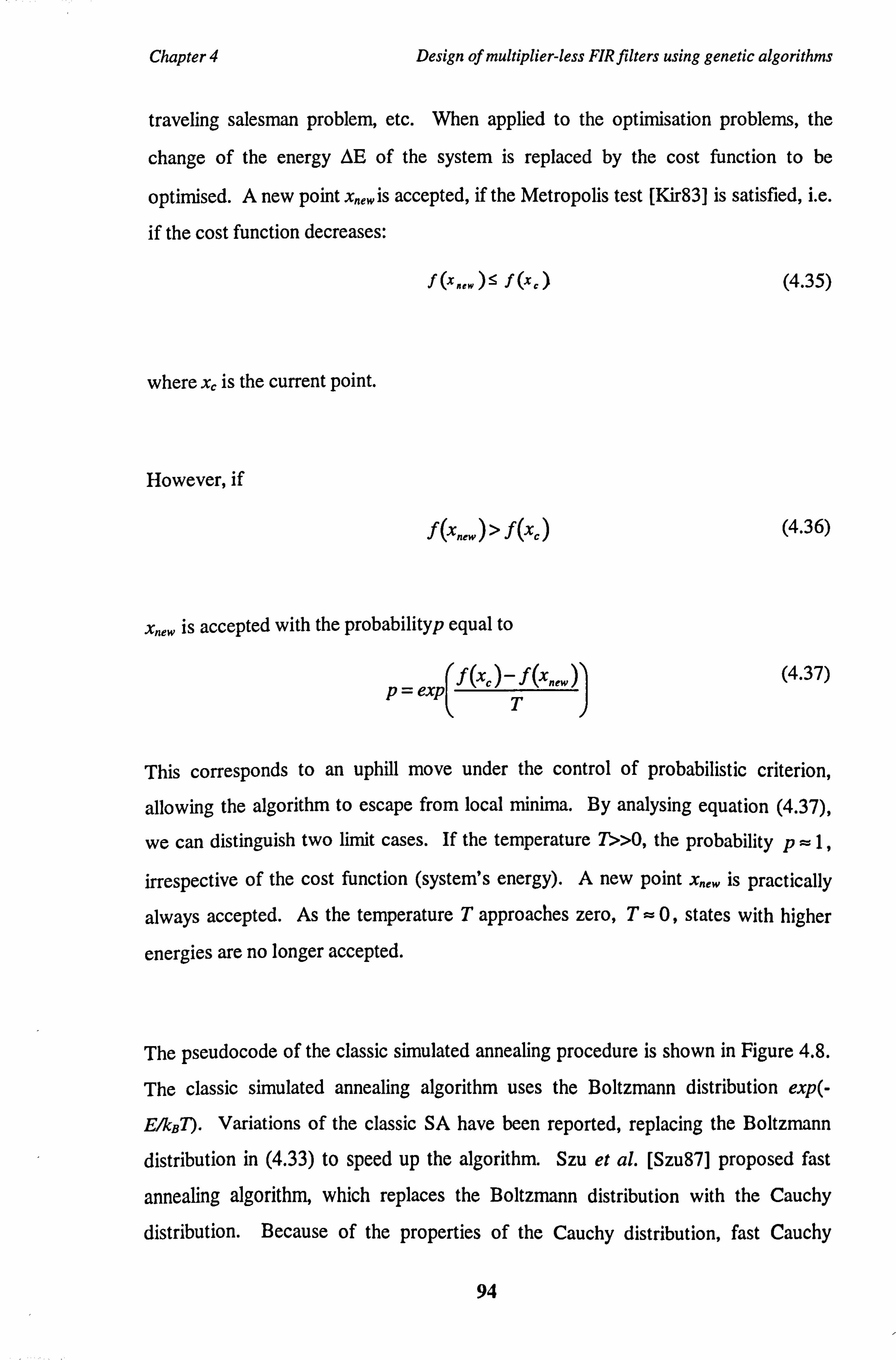
Chapter 4 Design of multiplier-less FIR filters using genetic algorithms
traveling salesman problem, etc. When applied to the optimisation problems, the
change of the energy DE of the system is replaced by the cost function to be
optimised. A new point xneW is accepted, if the Metropolis test [Kir83] is satisfied, i. e.
if the cost function decreases:
f (x. ) sf (xý) (4.35)
where x, is the current point.
However, if
f (xnew) >f
(xc) (4.36)
x,,,,, is accepted with the probabilityp equal to
p=exp f(xc)-J (xnew) (4.37)
T
This corresponds to an uphill move under the control of probabilistic criterion,
allowing the algorithm to escape from local minima. By analysing equation (4.37),
we can distinguish two limit cases. If the temperature 7'>>O, the probability p =1,
irrespective of the cost function (system's energy). A new point Xnew is practically
always accepted. As the temperature T approaches zero, T=0, states with higher
energies are no longer accepted.
The pseudocode of the classic simulated annealing procedure is shown in Figure 4.8.
The classic simulated annealing algorithm uses the Boltzmann distribution exp(-
E/kBT). Variations of the classic SA have been reported, replacing the Boltzmann
distribution in (4.33) to speed up the algorithm. Szu et al. [Szu87] proposed fast
annealing algorithm, which replaces the Boltzmann distribution with the Cauchy
distribution. Because of the properties of the Cauchy distribution, fast Cauchy
94

Chapter 4 Design of multiplier-less FIR filters using genetic algorithms
annealing (FCA) have an annealing schedule exponentially faster than classic
Boltzmann annealing. Further improvement of FCA was proposed by Ingber
[Ing92]. Ingber claims that his method of very fast simulated reannealing (VFSR) is
exponentially faster than the fast Cauchy annealing and is also statistically guaranteed
to find the function optima.
Simulated Annealing ()
begin
initialise
for each temperature do
for number of search moves do
create new point x�ew=Xc + step
if Metropolis test passed then
accept new point
compare with optimal point x0
end if
adjust step
end for
decrease temperature
end for
if termination test passed then
return xop,
else
restart SA from xot
end if
end
Fig. 4.8 Pseudo-code of Simulated Annealing procedure
95

Chapter 4 Design of multiplier-less FIR filters using genetic algorithms
4.4.2 ML FIR filter design using simulated annealing
Because of its hill-climbing properties and the advantage to escape from local
minima, several authors attempted to use simulated annealing for design of digital
filters. Diethorn et al. [Die86] used simulated annealing for of finite wordlength
digital filters and his work has been later extended by Benvenuto et al. [Ben89a,
Ben89b]. Benvenuto et al. applied simulated annealing also in design of multiplier-
less FIR digital filters [Ben90, Ben92]. However, their approach is based on refining
of infinite precision coefficients obtained by Remez algorithm, that might limit
searching space that is explored by simulated annealing. We have shown earlier, that
genetic algorithm can produce better coefficient vectors than methods that use
infinite precision coefficients as a starting point. Finally, Cemes et al. proposed
simulated annealing as a technique for fine tuning of filter coefficients obtained by
genetic algorithm [Cem93d].
We propose a hybrid technique for the design of ML FIR filters based on robust
genetic algorithm kernel and simulated annealing operator. Genetic algorithm is used
to rapidly explore the discrete space of power-of-two coefficients. We have
implemented advanced genetic algorithms using tournament selection [Go191 ], two-
point crossover [Cav70], linear fitness scaling [Gol89a] and steady-state generation
replacement [Dav91] that is retaining the elite chromosome. In each generation, the
elite chromosome is selected and simulated annealing is applied. We follow the same
annealing schedule as in [Ben92]. Pseudo-code of the proposed hybrid algorithm
(GA-3) is shown in Figure 4.9.
96

Chapter 4 Design of multiplier-less FIR f lters using genetic algorithms
Hybrid GA-SA Genetic Filter Design ()
begin
*/filter specification */
specify the frequency response, filter type and coefficient type
while no acceptable solution was found do
create the initial population of chromosomes
evaluate fitness of chromosomes
while not converged do
for each generation do
select parent chromosomes for recombination
perform crossover
perform mutation
evaluate fitness of offspring chromosomes
find elite chromosome
run simulated annealing on elite chromosome
steady-state replacement
insert elite chromosome into new population
end for
end while
/* increment the length of filter and run GA again
if no acceptable solution was found
increment the length of filter
end if
end while
end
Fig. 4.9 Pseudo-code of the hybrid GA-SA filter design algorithm
97

Chapter 4 Design of multiplier-less FIR filters using genetic algorithms
The hybrid GA-3 algorithm was compared with both simple and knowledge-based
genetic algorithms. Results have indicated that GA-3 algorithm is superior to GA-1
and GA-2 algorithms, especially for high-order filters. Figure 4.10 illustrates the
frequency responses for the low-pass filter LP2 designed using GA-1 and GA-3
algorithms. The dotted line represents the frequency response that has been achieved
by using GA-1 algorithm, while the solid line represents the frequency response that
have been achieved by fine tuning of the coefficient vector using GA-3 algorithm. A
similar frequency response to that obtained with the GA-1 algorithm has been
obtained with the GA-2 algorithm.
10
0
-10
-20
L -30 2
-40
-50
-60
-70 0 0.1 0.2 0.3 0.4 0.5 Normalised Frequency
Fig. 4.10 Frequency responses of the low-pass filter LP2 designed using GA-1 and
GA-3 algorithms
98

Chapter 4 Design of multiplier-less FIR filters using genetic algorithms
4.5 Conclusions
The results presented in this chapter have shown the superiority of genetic algorithms
for the design of FIR digital filters with discrete coefficients limited to power-of-two
values. They confirmed our expectations and conclusions drawn in Chapter 3.
Although limited to the simple genetic algorithm, the performance of the designed
algorithm is dramatic when compared to conventional techniques. Further
improvements of the basic technique have been also developed. They include
knowledge-based genetic algorithm and hybrid technique based on genetic algorithm
kernel using the simulated annealing operator that outperform design techniques
based on a simple genetic algorithm mainly for high-order filters.
99

r,
Chapter 5
Prediction of minimum filter length
Several methods for multiplier-less FIR filter design have been described in previous
chapters. The majority of the design methods are iterative in a sense that the
minimum filter length that is required to satisfy the filter specification is not known in
advance. In this chapter, we attempt to fill-in this knowledge gap and to devise a
formula that would predict the minimum number of power-of-two coefficients. The
techniques of genetic programming and symbolic regression are used to evolve the
formula describing the relationship between the filter length and its specification. The
rest of this chapter is organised as follows. First, Kaiser's empirical formula that is
used to estimate a number of infinite precision filter coefficients is described. The
technique of genetic programming and symbolic regression is briefly introduced next.
Section 6.3 describes our experiments and the results achieved. The chapter finishes
with conclusions.
100

Chapter 5
6.1 Kaiser's formula
Prediction of minimum filter length
A common drawback of all methods for the design of filters with power-of-two
coefficients is that the filter length is not known prior to the design procedure.
Therefore most designers adopted iterative design approach where design algorithms
operate between lower and upper boundaries on the filter length. The upper
boundary is set to the highest filter length that is still acceptable. The lower bound is
estimated using the empirical formula that has been devised by Kaiser and can be
found in classic DSP textbooks [Rab75]. Kaiser's formula has two different forms
depending on whether the windowing design method (5.1) or equiripple design
method (5.2) has been used:
N= -201og, 06 - 7.95 +1
14.360f (5.1)
N= -201og, o S, S2 -13 +1 14.6Af (5.2)
where 51952 are the frequency response ripples (they might be different when the
equiripple design method is used) and Of is the width of the transition band.
It should be noted that Kaiser's empirical formulas (5.1) and (5.2) have been devised
for infinite-precision coefficients. When filters are realised using power-of-two
coefficients only, the minimum number of coefficients is usually much higher,
rendering (5.1) and (5.2) only partially useful. Another disadvantage associated with
the use of (5.1) and (5.2) in the design of PWR2 filters is that the widely adopted
iterative approach starting from lower boundary on filter length is both time
consuming and costly. If some formula estimating the minimum filter length from the
filter specification would be known, it could save many unnecessary iterations
independently of the design method. This would be particularly useful for higher
BOURNEMOOUI 101
UNIVERSIT II rn rrA Y%r r
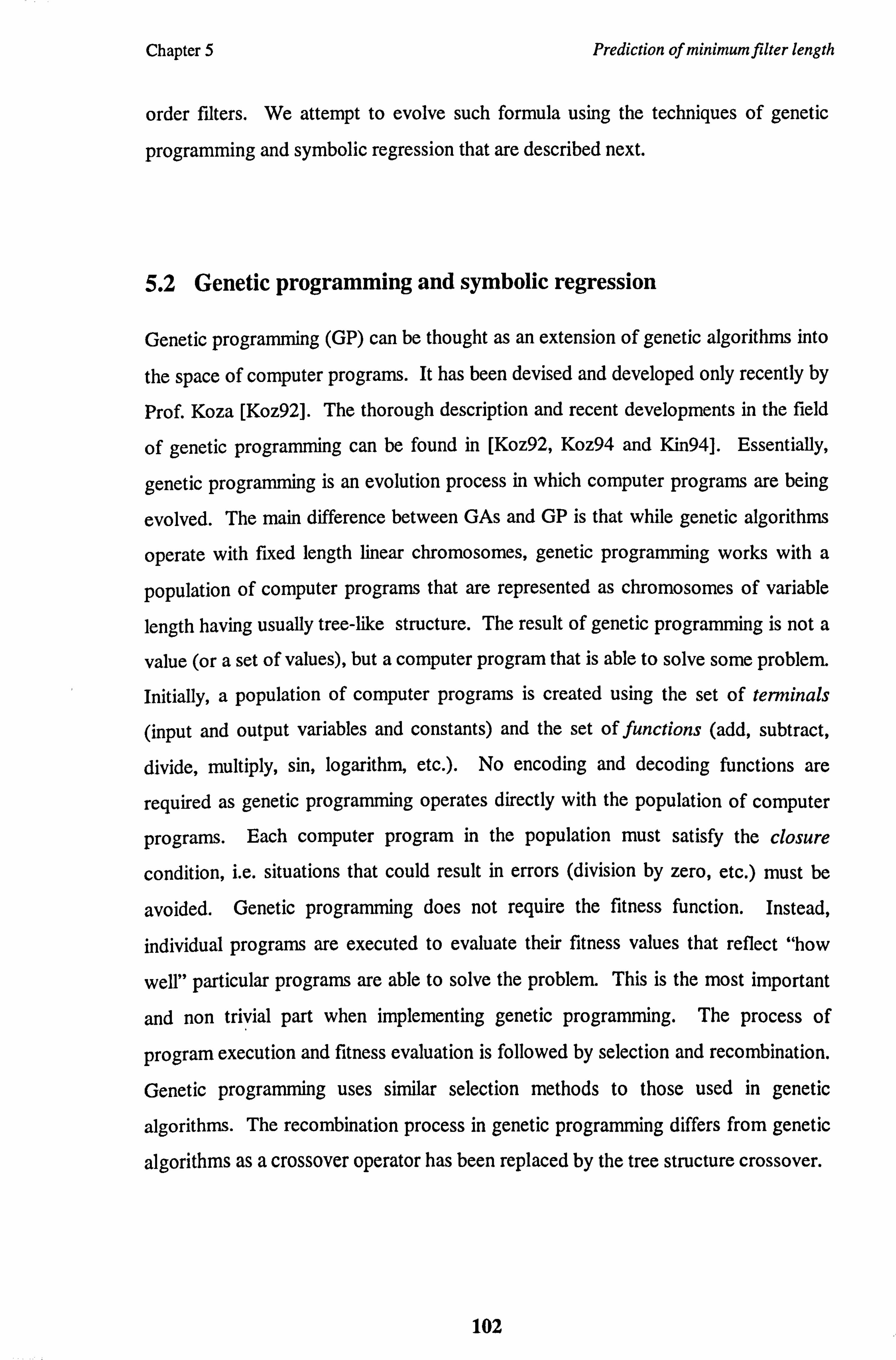
Chapter 5 Prediction of minimum filter length
order filters. We attempt to evolve such formula using the techniques of genetic
programming and symbolic regression that are described next.
5.2 Genetic programming and symbolic regression
Genetic programming (GP) can be thought as an extension of genetic algorithms into
the space of computer programs. It has been devised and developed only recently by
Prof. Koza [Koz92]. The thorough description and recent developments in the field
of genetic programming can be found in [Koz92, Koz94 and Kin94]. Essentially,
genetic programming is an evolution process in which computer programs are being
evolved. The main difference between GAs and GP is that while genetic algorithms
operate with fixed length linear chromosomes, genetic programming works with a
population of computer programs that are represented as chromosomes of variable
length having usually tree-like structure. The result of genetic programming is not a
value (or a set of values), but a computer program that is able to solve some problem.
Initially, a population of computer programs is created using the set of terminals
(input and output variables and constants) and the set of functions (add, subtract,
divide, multiply, sin, logarithm, etc. ). No encoding and decoding functions are
required as genetic programming operates directly with the population of computer
programs. Each computer program in the population must satisfy the closure
condition, i. e. situations that could result in errors (division by zero, etc. ) must be
avoided. Genetic programming does not require the fitness function. Instead,
individual programs are executed to evaluate their fitness values that reflect "how
well" particular programs are able to solve the problem. This is the most important
and non trivial part when implementing genetic programming. The process of
program execution and fitness evaluation is followed by selection and recombination.
Genetic programming uses similar selection methods to those used in genetic
algorithms. The recombination process in genetic programming differs from genetic
algorithms as a crossover operator has been replaced by the tree structure crossover.
102

Chapter 5 Prediction of minimum filter length
The process of program execution, fitness evaluation, selection and recombination is
repeated for a given number of generations. With the exception of program
execution stage, the process is identical to genetic algorithms. Pseudo-code of
genetic programming is illustrated in Figure 5.1, while the tree structure crossover is
shown in Figure 5.2.
Genetic Programming( )
begin
identify set of functions and terminals
randomly create population of computer programs
while termination criterion is not satisfied do
for each generation do
execute each program to evaluate its fitness
for each program do
select genetic operator (crossover, mutation, reproduction)
perform genetic operator
end for
end for
end while
end
Fig. 5.1 Pseudo-code of genetic programming
Genetic programming has been successfully applied to a wide range of problems that
are difficult to solve, including prediction of protein characteristics, forecasting of the
weather, automatic programming, image compression, etc. Amongst a number of
successful applications of genetic programming, we are particularly interested in
symbolic regression (SR) described by Koza [Koz92]. Koza defines symbolic
regression as "seeking for a mathematical expression that would approximately fit a
given sample of data". Symbolic regression is different from the polynomial
103
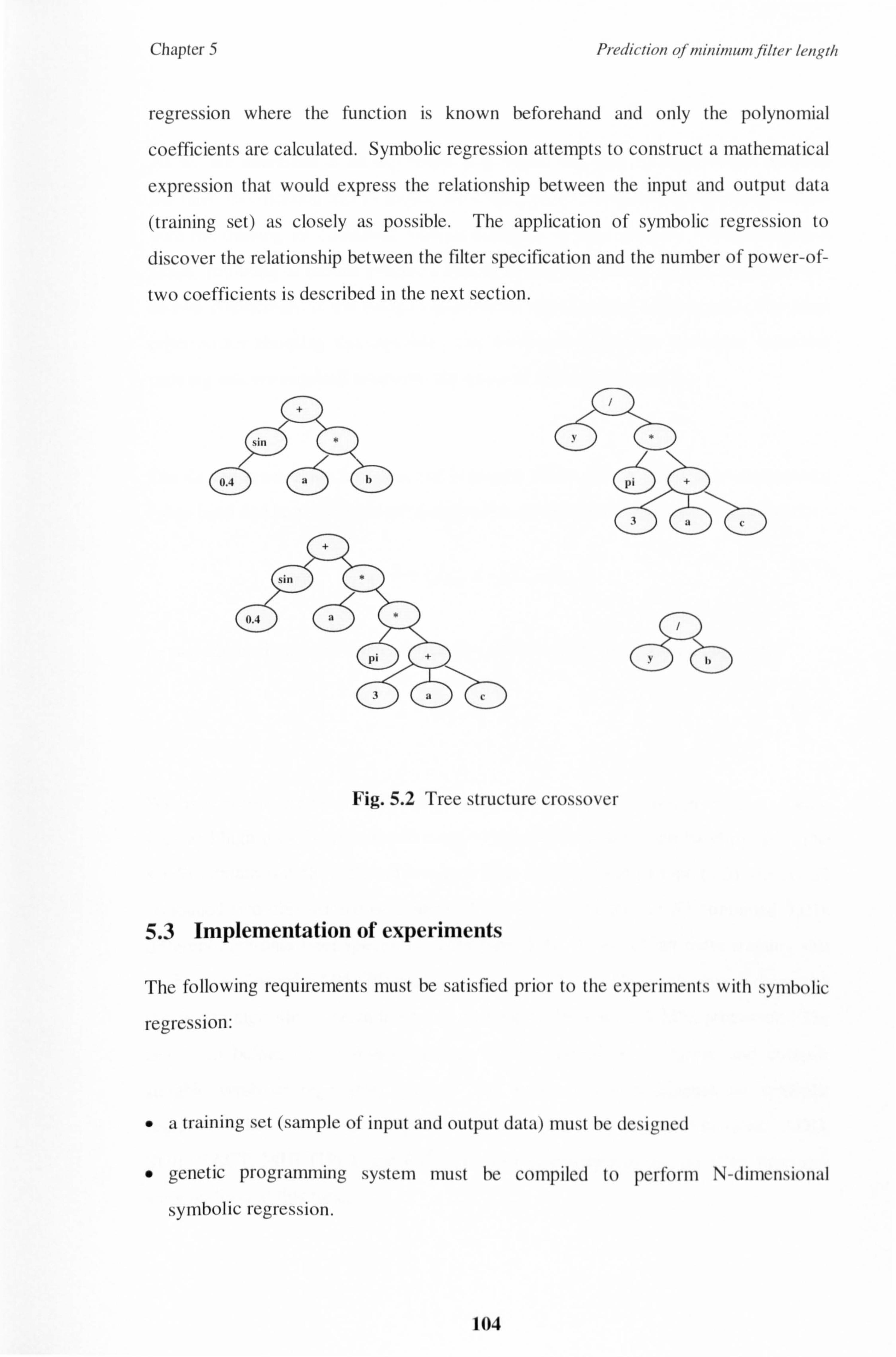
Chapter 5 Predicviail of imnimi wn filter length
regression where the function is known beforehand and only the polynomial
coefficients are calculated. Symbolic regression attempts to construct a mathematical
expression that would express the relationship between the input and output data
(training set) as closely as possible. The application of symbolic regression to
discover the relationship between the filter specification and the number of power-of-
two coefficients is described in the next section.
sin "
0.4 (a1 i'
Yb
Fig. 5.2 Tree structure crossover
5.3 Implementation of experiments
The following requirements must be satisfied prior to the experiments with symbolic
regression:
"a training set (sample of input and output data) must be designed
" genetic programming system must he compiled to perform N-dinlensional
symbolic regression.
104

Chapter 5 Prediction of minimum filter length
As we are interested in an expression that would describe the relationship between
the filter specification and its length, we must provide the symbolic regression system
with the training set containing various examples of filter designs. We have chosen
simple rounding of infinite precision Remez coefficients to the nearest single power-
of-two coefficients as the design algorithm to construct the training set. The main
criterion for choosing this algorithm was its simplicity and the speed, as extensive
training sets are required to sample the space of filter specifications.
The design space S for low-pass and high-pass filters can be either four-dimensional
(pass-band and stop-band cut-off frequencies and pass-band and stop-band ripples):
ý' Spass 9k op
(5.3) `S - fpars
ý Jstop +V
or two-dimensional (the width of transition band and the max. ripple allowed):
S= {Af, s} (5.4)
We have constructed three different training sets sampling the design space S of low-
pass and high-pass filters in broad range of cut-off frequencies and band ripples. The
set S1 contained 3,487 different low-pass filter specifications of type (5.3), the set S2
contained two-dimensional equivalent of the set Si and the set S3 contained 3,018
different high-pass filter specifications of type (5.4). To construct these training sets
we have performed 6,505 different filter designs in total. This took several days with
the design algorithm written in Matlab running on Pentium 120 Mhz processor. The
next step before the evolution process can be started is to choose and compile
suitable symbolic regression system We have chosen N-dimensional symbolic
regression that has been compiled with the following set of functions: ADD,
SUBTRACT, MULTIPLY and DIVIDE. For simplicity reasons, no other functions
were realised at this time.
105

Chapter 5 Prediction of minimum filter length
Upon completion of these preparatory steps, the process of five-dimensional (for the
set Si) and three-dimensional (for the sets S2 and S3) symbolic regression has been
performed. Symbolic regression in terms of memory and execution time is extremely
costly process. The time to finish our experiments varied from 8 to 14 days as shown
in Table 5.1. Each experiment has been repeated six times to produce more results
that would allow us to choose the most suitable expression and to compare different
runs. The results are analysed in the next section.
Table 5.1 Comparisons of SR runs
Dataset Training set Training set size Time to complete SR
cardinality
Si 5 3,487 14 days
S2 3 3,487 9 days
S3 3 3,018 8 days
5.4 Analysis of results
The mathematical expressions resulting from the application of symbolic regression
to the training sets Si, S2 and S3 are rather complex. This is because symbolic
regression does not simplify the evolved expressions from generation to generation.
This does not constitute a problem as we were mainly interested whether the
expression describing the relationship between the filter specification and its length
could be attained using the symbolic regression. We have performed the error
analysis of the resulting expressions to evaluate how close the evolved expressions
approximate the given training sets. For this purpose, the error has been defined as
the difference between the actual filter length and its estimated length.
106
Chapter 5 Prediction of minimum filter length
The error analysis of six different expressions that have been evolved by the five-
dimensional symbolic regression using the training se61 is shown in Figure 5.3.
Ui W
50 Co
so
00 50 III
ID Eqi bon EQll1
ö t w
b
Equaton EW-3
w w
--0 500 1000 1500 2000 2500 3000 3500
Equation EOU-5
g W
w W
260
zoo
160
100
60
0
LL
o 600 1000 1500 2000 2500 8000 3600
Equatlon EQU-6
Fig. 5.3 Error analysis of expressions EQU-1 to EQU-6 for estimating the filter
length for low-pass filters (five-dimensional training set)
107
--o coo 1000 1900 2000 2500 3000 3500
Equation EOU-2
15 2 000 2500 3000 3500 Equation EOU-4

Chapter 5 Prediction of minimum filter length
Studies of the error analysis and the corresponding training sets have shown that
large errors, represented as peaks in Figure 5.3, have occurred mainly for high-order
filters. As the high-order filters (with the actual filter length bigger than 50)
represented less than 5% of the entire training set, we have removed them from the
training set S1 and re-evaluated the error analysis. In these circumstances the
evolved expressions produced more realistic results. The maximum and average
errors for the expressions EQU-1 to EQU-6 are shown in Table 5.2. The error
analysis for the expression EQU-3 that yields in lowest errors is illustrated in Figure
5.4.
Table 5.2 Maximum and average errors following the removal of high-order filters
Expression Maximum error Average error
EQU-1 32.60 0.2162
EQU-2 33.35 0.2387
EQU-3 32.22 0.0988
EQU-4 32.76 0.1600
EQU-5 33.70 0.4355
EQU-6 34.31 2.3418
108

Chapter 5
40
30
20
10
W 0
-10
-20
-30 0 500 1000 1500 2000 2500 3000 3500
Equation EQU-3 (high-order filters removed)
Fig 5.4 Error analysis of expression EQU-3 following the removal of high-order
filters
The equation EQU-3 evolved by the five-dimensional symbolic regression using the
training set Si that contained 3,487 filter designs is as follows:
Nestimated = (fstop'fpass) - (((fpasl(2*(fstop'fpass)))*fpass)/fstop) + fstop
Prediction of minimum filter length
+ (((fstop'2*fpass)-(fp. /SS))-i(fp. Jfstop)/(fstop*fstop)))/6
+ fpass/(fstap* ftop*Ss) +2 *Sp- fpasifstop
+ 5ý ((Estop'((fpass/fstop)/(fstop*fstop)))/fstop)) + i(('stop*(fstop'fpass))-fpass)
+ (((fpasJ(((fstop'fpass)-(fstop*fstop))+Ss))*fpass)/(fstop'fpass))
+ ((SS ((fP jSs)*'pass))-fsýoP)/(2*SS)
(5.5)
109

Chapter 5 Prediction of minimum filter length
The equation (5.5) has been tested with the set of filters not contained in the training
set. Table 5.3 shows comparisons between the actual filter length, the filter length
estimated using the Kaiser's formula and the equation (5.5) evolved using symbolic
regression.
Table 5.3 Comparison of Kaiser formula, Maximum and average errors following
the removal of high-order filters
fpass Estop Sp 88s NKaiser Nestimated Nactual
0.02 0.2 0.1 0.1 4 6 15
0.2 0.3 0.2 0.2 2 10 10
0.2 0.4 0.1 0.1 3 10 10
0.316 0.432 0.18 0.10 4 38 16
0.316 0.432 0.18 0.12 3 25 20
0.183 0.375 0.1 0.1 4 11 14
5.5 Conclusions
This chapter presents the application of symbolic regression to discovery of filter
length when the filter coefficients are restricted to single power-of-two only. Several
expressions describing approximate relationship between the filter specification and
its length have been evolved. The error analysis has shown that the results are
reasonably good for low-order filters (filter length N: 5 30). Although the training set
for symbolic regression contained large amount of data, higher order filters (N>30)
represented less than 5% of the training set. This could explain large difference
110

Chapter 5 Prediction of minimum filter length
between the actual and estimated filter length for higher order filters. Further work is
required to evolve a simplified expression that would achieve high accuracy.
However, any of the evolved equation EQU-1 to EQU-6 can be included in any
design technique for filters with single power-of-two coefficients in the present form.
To increase the accuracy of the expressions, two alternatives are possible, including
adding more functions into the function set and using better methods to generate the
training set. This constitutes the aim of our future research.
111

Chapter 6
Conclusions and future work
The aim of this chapter is to review achievements that have been made and the
contribution of this research work to the field of multiplier-less FIR filter design.
Novel approaches to the design of multiplier-less FIR filters with coefficient vectors
limited to power-of-two terms that have been proposed in this thesis can be classified
into three separate classes:
" improvements of calculus-based design methods,
" design of ML FIR filters based on evolutionary algorithms,
" evolution of the formula for estimation of ML FIR filter length.
The advances that have been made and the limitations of the developed algorithms
are analysed in the next section. The chapter concludes with a suggestions for further
research to enhance proposed techniques.
112

Chapter 6 Conclusions and future work
6.1 Summary of the results
Two novel design techniques have been developed following the analysis of available
calculus-based methods. The first technique has been referred to as evolutionary
local search (ELS). ELS is a combination of exhaustive search with a refined local
search technique. The algorithm differs from the majority of calculus-based
techniques as it does not require the initial set of infinite-precision filter coefficients
as a starting point. Although the algorithm is simple in its principle, it can design
optimal low-order ML FIR and sub-optimal higher-order filters. It has outperformed
the traditional rounding of infinite-precision filter coefficients.
The second technique has been termed as MSE coefficient sensitivity based
rounding. In our view, this technique represents development of one of the best
classic design techniques for ML FIR filter design available. We have suggested
improvements to the basic technique to include among other types the design of
filters with multiple-bands. Major improvements stem from the replacement of the
original sensitivity criterion with the mean square error sensitivity criterion. The
results that have been achieved and presented have demonstrated the superiority of
this design technique. However, both ELS and MSE coefficient sensitivity based
rounding techniques are able to produce only suboptimal designs as they limit
searching to the vicinity of the starting vector.
Our work in the field of multiplier-less FIR filter design using genetic algorithms
represents one of the earliest works in the field. Several novel algorithms, named as
GA-l, GA-2 and GA-3, have been proposed. The kernel of these algorithms is based
on a simple genetic algorithm model. The GA-1 algorithm uses unique encoding
scheme that guarantees that each population contains only valid chromosomes
without adverse effects on the performance of genetic algorithm The GA-1
algorithm has been compared with other techniques, namely with the rounding of
infinite precision coefficients based on MSE coefficient sensitivity criterion. Results
have indicated that the GA-1 algorithm has greatly outperformed traditional ML FIR
113

Chapter 6 Conclusions and future work
filter design techniques as further reduction of the filter complexity has been
achieved. It has to be stressed at this point that the filter vectors that have been
designed using GA-1 algorithm could not be designed using other techniques that are
based on rounding of infinite precision coefficients, as these techniques limit the
searching space to the vicinity of infinite precision coefficients only. The power of
the GA-1 algorithm to explore the entire searching space is its main advantage
opposite calculus-based algorithms. Even better results have been achieved with GA-
2 algorithm that uses inserting of knowledge-based chromosome into the initial
population. Here, the knowledge based chromosome represents a Remez coefficient
vector rounded to nearest single power-of-two coefficients. To overcome the
problem of premature convergence, fitness scaling has been applied.
Hybrid evolutionary techniques are represented by GA-3 algorithm. The kernel of
GA-3 algorithm embodies powerful genetic algorithm with a class of advanced
genetic operators and simulated annealing. Here, the main genetic kernel is used to
explore searching space rapidly, while simulated annealing is applied to refine the
solution that has been obtained with genetic algorithms. GA-3 algorithm
outperforms GA-1 and GA-2 mainly for higher-order filters. However, there is a
price to be paid for the algorithm's ability to explore N-dimensional searching space
as many control parameters have to be tuned.
A common drawback of all design methods that have been presented is that the filter
length, i. e. the number of coefficients that is required to satisfy the filter specification,
is not known beforehand. Instead, lower and upper boundaries on the filter length
are specified and design techniques work iteratively within these boundaries. It
would be advantageous to have a formula that would be able to estimate the filter
length from its specification. In the last chapter, we have shown that it is possible to
evolve such formula using the technique of genetic programming and symbolic
regression. Although the expression that has been evolved is rather approximate, it
does compare very well with Kaiser's formula that is used in majority of FIR filter
design methods, either calculus-based or based on evolutionary algorithms. The
114

Chapter 6 Conclusions and future work
accuracy of the formula can by further improved either by extending the function set
that is used by symbolic regression or using mixed integer linear programming to
create a training set that would contain optimal coefficient vectors.
6.2 Further work
The aims of this research work as stated in Chapter 1 have been accomplished.
However, the research has uncovered some problems that need to be addressed. We
have shown that genetic algorithms are robust optimisation techniques, but they can
suffer from undesired effects, such as premature or slow convergence. To overcome
these problems, we suggest to use robust genetic kernels based on distributed genetic
algorithms (DGA) described by Tanese in [Tan89]. Distributed genetic algorithms
operate with several populations of chromosomes, with each population having
different control parameters and using different genetic operators. Initially, there is
no interaction between the populations. After a pre-specified number of generations,
the average fitness values of different populations are compared and genetic
operators that are related to the best performing population are selected for further
evolution process.
Finally, the use of genetic programming for the design of multiplier-less FIR filters
should lead to further improvements, as the filter coefficients and the filter
architecture can be evolved at the same time. The approach using genetic
programming would further benefit from variable length chromosome representation,
effectively exploring the searching space between lower and upper boundaries in
highly parallel fashion. The novel techniques that have been presented in this thesis
can be also extended to the design of multiplier-less infinite impulse response filters.
115

References
[Aru93] Arunkumar, S., and Chockalingam, T.: `Genetic search algorithms and
their randomized operators', Computers and Mathematics with
applications, No. 5,1993, pp. 91-100
[Ben89a] Benvenuto, N., and Marchesi, M.: A.: `Digital filter design by simulated
annealing', IEEE Trans. on Circuits and Systems, Vol. 36, No. 3, pp. 459-
460 (March 1989)
[Ben89b] Benvenuto, N., Marchesi, M., Orlandi, G., Piazza, F., and Uncini, A.:
`Finite wordlength digital filter design using an annealing algorithm',
Proc. of Int. Conference on Acoustics, Speech and Signal Processing,
Glasgow, UK, Vol. 2, pp. 861-864 (May 1989)
[Ben90] Benvenuto, N., Marchesi, M., and Uncini, A.: `Results on the application
of simulated annealing algorithm for the design of digital filters with
powers-of-two coefficients', Proc. of Int. Conference on Acoustics,
Speech and Signal Processing, Albuquerque, USA, Vol. 3, pp. 1301-
1304 (April 1990)
[Ben92] Benvenuto, N., Marchesi, M., and Uncini, A.: `Applications of simulated
annealing for the design of special digital filters', IEEE Trans. on Signal
Processing, Vol. 40, No. 2, pp. 323-332 (February 1992)
[Bu187] Bull, D. R., and Horrocks, D. H.: `Reduced complexity digital filtering
structures using primitive operations', Electronics Letters, Vol. 23,
No. 15,1991, pp. 7699-7771
116

[Bu188] Bull, D. R., and Horrocks, D. H.: `Primitive operator digital filter
synthesis using a shift biased algorithm', IEEE Int. Symposium on
Circuits and Systems, Helsinki, Finland, June 1988, pp. 1529-1532
[Bu191] Bull, D. R., and Horrocks, D. H.: `Primitive operator digital filters', IEE
Proceedings-G, Vol. 138, No. 3, pp. 401-411 (June 1991)
[Cav7O] Cavicchio, D. J.: Adaptive search using simulated evolution, unpublished
doctoral dissertation, University of Michigan, Ann Arbor
[Cem93a] Cemes, R., and Ait-Boudaoud, D.: `Modified sensitivity criterion for the
design of powers-of-two FIR filters', Electronics Letters, Vol. 29,
No. 16, pp. 1467-1469 (August 1993)
[Cem93b] Cemes, R., and Ait-Boudaoud, D.: `Genetic approach to the design of
multiplier-less FIR filters', Electronic Letters, Vol. 29, No. 24, pp. 2090-
2091 (November 1993)
[Cem93c] Cemes, R., and Ait-Boudaoud, D.: 'Multiplier-less FIR filter design with
power-of-two coefficients', Thirteenth Saraga Colloquium on digital and
analogue filters and filtering systems, 2nd November 1993, London
[Cem93d] Cemes, R., Ait-Boudaoud, D., and Holloway, S.: `Evolutionary adaptive filtering, International Conference on Artificial neural Networks and Genetic Algorithms, Ales, France, 18th-21 st April 1995
[Dav9l] Davis, L.: Handbook of Genetic Algorithms, Van Nostrand Reinhold,
1991
[DeJ75] DeJong, K.: The analysis and behaviour of a class of genetic adaptive
systems. PhD thesis, University of Michigan, 1975
117

[DeJ90] DeJong, K. A., and Spears, W. M.: `An analysis of the interacting roles of
population size and crossovber in genetic algorithms', Proc. First
Workshop Parallel Problem Solving from Nature, Springer-Verlag,
Berlin, 1990, pp. 38-47
[Die86] Diethorn, E. J., and Munson, D. C.: `Finite word length FIR digital filter
design using simulated annealing', Proc. IEEE Int. Symp. on Circuits and
Systems, San Jose, pp. 217-220 (May 1986)
[Gen94] Gentilli, P., Piazza, F., and Uncini, A.: `Evolutionary design of FIR
digital filters with power-of-two coefficients', Proceedings of the First
IEEE Conference on Evolutionary Computation, Orlando, Florida, USA,
1994
[Gha93] Ghanekar, S., Tantaratana, S., and Franks, L. E.: `Design and architecture
of multiplier-free FIR filters using periodically time-varying ternary
coefficients', IEEE Trans. on Circuits and Systems - I, Vol. 40, No. 5,
pp. 364-370 (May 1993)
[Gha94] Ghanekar, S., Tantaratana, S., and Franks, L. E.: `Multiplier-free IIR
filter realization using periodically time-varying state-space structure',
IEEE Trans. on Signal Processing, Vol. 42, No. 5, pp. 1008-1025 (May
1994)
[Go189a] Goldberg, D. E.: Genetic algorithms in search, optimization, and
machine learning, Addison-Wesley Publishing Company, Inc., USA,
1989
[Go189b] Goldberg, D. E.: Genetic algorithms and Walsh functions: Part I, a gentle
introduction, Complex systems, Vol. 3,1989, pp. 129-152
118

[Go190] Goldberg, D. E.: Real-coded genetic algorithms, virtual alphabets, and
blocking, IlliGAL Report No. 90001,
ftp: //gal4. ge. uiuc. edu/pub/papers/I11iGALs/90001. ps. Z
[Go191] Goldberg, D. E., and Deb, K.: 'A comparative analysis of selection
schemes used in genetic algorithms'. in the book Foudations of Genetic
Algorithms, (Edited by G. J. E. Rawlins), Morgan Kaufmann Publishers,
San Mateo, California, 1991, pp. 69-93
[Go192] Goldberg, D. E., Deb, K., and Clark, J. H.: 'Genetic algorithms, noise and
the sizing of populations'. Complex systems, Vol. 6, Part. 4,1992, pp. 333-
362
[Gre85) Greenberger, A. J.: `Digital tranversal filter architecture', Electronic
Letters, Vol. 21, No. 3, pp. 86-88 (January 1985)
[Gre86] Grefenstette, J. J.: `Optimisation of control parameters for genetic
algorithms', IEEE Trans. Systems, Man, and Cybernetics, Vol. SMC-16,
No. 1, pp. 122-128 (Jan. /Feb. 1986)
[Ho171] Hollstien, R. B.: `Artificial Genetic Adaptation in Computer Control
Systems', PhD thesis, University of Michigan, 1971
[Ho175] Holland, J. H.: Adaptation in natural and artificial systems, The
University of Michigan Press, Ann Arbor, Michigan, USA, 1975
[Hwa79] Hwang, K.: Computer arithmetic, principles, architecture, and design,
New York: Wiley, 1979
119
[Ife93] Ifeachor, E. C., and Harris, S. P.: 'A new approach to frequency sampling
filter design using genetic algorithms'. Natural Algorithms in Signal
Processing, Workshop at Danbury Park Conference Centre, Chelmsford,
UK, November 1993
[Ing92] Ingber, L.: `Genetic Algorithms and very fast Simulated Reannealing: A
comparison', Mathematical and Computer Modelling, 16(11), pp. 87-100
(1992)
[Kai77] Kaiser, J. F., and Hamming, R. W.: `Sharpening of the response of
symmetric nonrecursive filter by multiple use of the same filter', IEEE
Trans. Acoustics, Speech, Signal Processing, Vol. ASSP-25, pp. 415-422
(October 1977)
[Kin71] Kingsbury, N. G., and Rayner, P. J. W.: `Digital filtering using logarithmic
arithmetic', Electronics Letters, Vol. 7, No. 2, pp. 56-58 (January 1971)
[Kin89] King, R., Ahmadi, M., Gorgui-Naguib, R., Kwabwe, A., and Azimi-
Sadjadi, M.: Digital filtering in one and two dimensions, Plenum Press,
New York, 1989
[Kin94] Kinnear, E. Jr.: Advances in genetic programming, MIT Press,
Cambridge, Massachusetts, 1994
[Kir83] Kirkpatrick, S., Gelatt, C. D., and Vecchi, M. P.: `Optimisation by
simulated annealing', Science, Vol. 220, No. 4598, pp. 671-680 (13 May
1983)
[Kod80] Kodek, D. M.: `Design of optimal finite wordlength FIR digital filters
using Integer Programming techniques', IEEE Transactions on
Accoustics, Speech, and Signal Processing, Vol. ASSP-28, No. 3,
pp. 304-308 (June 1980)
120
[Kod8l] Kodek, M. D., and Steiglitz, K.: 'Comparison of optimal and local search
methods for designing finite wordlength FIR digital filters', IEEE Trans.
on Circuits and Systems, Vol. CAS-28, No. 1, pp. 28-32 (January 1981)
[Koz92] Koza, J. R.: Genetic Programming: On the programming of computers
by means of natural selection, MIT Press, Cambridge, Massachusetts,
1992
[Koz94] Koza, J. R.: Genetic Programming II: Automatic discovery of reusable
programs, MIT Press, Cambridge, Massachusetts, 1994
[Lim79] Lim, Y. C., and Constantinides, A. G.: `Linear phase FIR digital filter
without multipliers', Proc. 1979 IEEE Int. Symp. Circuits and Systems,
pp. 185-188
[Lim82] Lim, Y. C., Parker, S. R., and Constantinides, A. G.: `Finite word length
FIR filter design using integer programming over a discrete coefficient
space', IEEE Trans. on Acoustics, Speech, and Signal Processing, Vol.
ASSP-30, No. 4, pp. 661-664 (August 1982)
[Lim83a] Lim, Y. C., and Parker, S. R.: `FIR filter design over a discrete powers-of-
two coefficient space', IEEE Trans. on Acoustics, Speech, and Signal
Processing, Vol. ASSP-31, No. 3, pp. 583-591 (June 1983)
[Lim83b] Lim, Y. C., and Parker, S. R.: 'Discrete coefficient FIR digital filter design
based upon an LMS criteria', IEEE Trans. on Circuits and Systems, Vol.
CAS-30, No. 10, pp. 723-739 (October 1983)
121

[Lim88] Lim, Y. C., and Liu, B.: Design of cascade form FIR filters with discrete
valued coefficients', IEEE Trans. on Acoustics, Speech, and Signal
Processing, Vol. 36, No. 11, pp. 1735-1739 (November 1988)
[Lim90] Lim, Y. C.: `Design of discrete-coefficient-value linear phase FIR filters
with optimum normalized peak ripple magnitude', IEEE Trans. on
Circuits and Systems, Vol. 37, No. 12, pp. 1480-1486 (December 1990)
[MC73a] McClellan, J. H., Parks, T. W.: `A unified approach to the design of
optimum FIR linear-phase digital filters', IEEE Transactions on Circuit
Theory, CT-20, pp. 697-701 (November 1973)
[MC73b] McClellan, J. H., Parks, T. W., and Rabiner, L. R.: `A computer program
for designing optimum FIR linear phase digital filters', IEEE
Transactions on Audio Electroacoustics, AU-21, pp. 506-526 (1973)
[Met53] Metropolis, N., Rosenbluth, S., Rosenbluth, M., Teller, A., and Teller,
E.: `Equations of state calculations by fast computing machines', J.
Chem. Phys., Vol. 21, pp. 1087-1091 (1953)
[Par72] Parks, T. W., and McClellan, J. H.: `Chebyshev approximation for
nonrecursive digital filters with linear phase', IEEE Transactions on
Circuit Theory, CT-19, pp. 189-194 (1972)
[Par87] Parks, T. W., and Burrus, C. S.: Digital filter design, John Wiley & Sons,
New York, 1987
[Rab72] Rabiner, L. R.: `Linear program design of FIR digital filters', IEEE Trans.
Audio Electroacoustics, 20, pp. 280-288 (October 1972)
122

[Ram89] Ramakrishnan, K. V., and Gopinathan, E.: `Design of FIR filters with
reduced computations', Circuits, Systems and Signal Processing, Vol. 8,
No. 1,1989, pp. 17-23
[Ree94] Reeves, C. R.: 'Genetic algorithms and combinatorial optimization',
Adaptive computing and information processing, Seminar held at Brunel
Conference Centre, London, January 25-77 1994, Unicorn Seminars
1994, pp. 711-723
[Rei65] Reif, F.: Fundamentals of statistical and thermal physics, New York,
McGraw-Hill, 1965
[Rem57] Remez, E. Ya.: `General computational methods of Tchebycheff
approximation', Atomic Translation 4491, pp. 1-85, Kiev, 1957
[Sam88] Samueli, H.: `The design of multiplier-less FIR filters for compensating
D/A converter frequency response distortion', IEEE Transactions on
Circuits and Systems, Vol. 35, No. 8, pp. 1064-1066 (August 1988)
[Sam89] Samueli, H.: `An improved search algorithm for the design of
multiplierless FIR filters with powers-of-two coefficients', IEEE
Transactions on Circuits and Systems, Vol. 36, No. 7, pp. 1044-1047
(July 1989)
[Sar9l] Saramäki, T.: `A systematic technique for designing highly selective
multiplier-free FIR filters', Proc. IEEE Int. Conf. Circuits Syst.,
Singapore 1991, pp. 484-487 (1991)
123

[Sch9l] Schraudolph, N. N., and Belew, R. K.: `Dynamic parameter encoding for
genetic algorithms', UCCD Technical Report CS 90-175, University of
California, San Diego (September 1991)
[Sha87] Shah, I. A., and Bhattacharya, A. K.: `A fast multiplierless architecture for
general purpose VLSI FIR digital filters', IEEE Trans. on Consumer
Electronics, Vol. CE-33, No. 3, pp. 129-135 (August 1987)
[Sha9l] Shaffeu, H., Jones, M. M., Griffiths, H. D., and Taylor, J. T.: `Improved
design procedure for multiplierless FIR digital filters', Electronics
Letters, Vol. 27, No. 13, pp. 1142-1144
[Sch89] Schaffer, J. D.: `A study of control parameters affecting on-line
performance of genetic algorithms for function optimization', Proc. of
the Third International Conference on Genetic Algorithms, Morgan
Kaufmann Publishing, San Mateo, California, 1989, pp. 51-60
[Sch93] Schaffer, J. D., and Eshelman, L. J.: `Designing multiplierless digital
filters using genetic algorithms', Proc. of the Fifth International
Conference on Genetic Algorithms, Morgan Kaufmann Publishing, San
Mateo, California, 1993, pp. 439-444
[Suc91] Suckley, D.: 'Genetic algorithm in the design of FIR filters', IEE
Proceedings-G, Vol. 138, No. 2, April 1991, pp. 234-238
[Suh87] Suh, J. Y., and Gucht, D. V.: 'Incorporating heuristic information into
genetic search', Proceedings of the Second International Conference on Genetic algorithms, (Edit. by J. J. Grefenstette), MIT, Cambridge, USA,
July 28-31,1987, Lawrence Erlbaum Associates, Hillsdale, USA,
pp. 100-107
124

[Szu87] Szu, H., and Hartley, R.: `Fast simulated annealing', Phys. Letters A,
Vol. 122 (3-4), pp. 157-162 (1987)
[Sys89] Syswerda, G.: 'Uniform crossover in genetic algorithms', Proceedings of
the Third International Conference on Genetic Algorithms, George
Mason University, June 4-7,1989, Morgan Kaufmann Publishers, Inc.,
San Mateo, California, pp. 2-9
[Tai92] Tai, Y. L., and Lin, T. P.: `Design of multiplierless FIR filters by multiple
use of the same filter', Electronics Letters, Vol. 28, No. 2, pp. 122-123
(January 1992)
[Tan89] Tanese, R.: `Distributed genetic algorithms', Proc. of the Third Int.
Conference on genetic Algorithms', ed. by J. D. Schaffer, Morgan
Kaufmann Publishers, 1989
[Wad90] Wade, G., Van-Eetvelt, P., and Darwen, H.: `Synthesis of efficient low-
order FIR filters from primitive sections', IEE Proceedings-G, Vol. 137,
No. 5, pp. 367 - 372 (October 1990)
[Wad94] Wade, G., Roberts, A., and Williams, G.: `Multiplier-less FIR filter
design using a genetic algorithm', IEE Proceedings - Vision, Image,
Signal Processing, Vol. 141, No. 3, pp. 175-180 (June 1994)
[Whi89] Whitley, D.: `The GENITOR algorithm and selection pressure: why
rank-based allocation of reproductive trials is best', Proceedings of the
Third International Conference on Genetic Algorithms (Edit. by
J. D. Schaffer), Morgan Kaufmann, 1989, pp. l 16-121
125

[Zha88] Zhao, Q., and Tadokoro, Y.: 'A simple design of FIR filters with powers-
of-two coefficients ; IEEE Transactions on Circuits and Systems, Vol.
35, No. 5, pp. 566-570 (May 1988)
126
Appendix A
Filter specifications
127

Filter type Number of Cutoff Desired Attenuation Maximum error
bands frequencies freq. resp. [dB] allowed
(f) (D) (S)
Bandpass 3 0-0.22, 0, > -26 dB 0.05,0.03,0.05
BP1 0.24-0.26, 1,
0.28-0.5 0
0-0.05, 1, 0.1,
Multiple bands 6 0.10-0.15, 0, 0.1,
MB1 0.20-0.23, 1, 0.1,
0.27-0.30, 0, 0.1,
0.35-0.4, 1, 0.1,
0.45-0.5 0 0.1
Multiple bands 0-0.04, 1, 0.1,
MB2 7 0.08-0.12, 0, 0.1,
0.16-0.22, 1, 0.1,
0.245 - 0.275, 0, 0.1,
0.30-0.34, 1, 0.1,
0.38-0.42, 0, 0.1,
0.46-0.5 1 0.1
Lowpass 2 0-0.27, 1, 0.02,
LP1 0.31-0.5 0 0.02
Lowpass 2 0-0.24, 1, 0.05,
LP2 0.25-0.5 0 0.05
Table A. 1 Some examples of filters designed using modified sensitivity criterion
128

Filter type Number of Cutoff Desired Weighting Maximum error
bands frequencies freq. resp. function allowed
(1) (D) W) (3)
Low-pass 2 0-0.25, 1, 1, 0.125,
GA-LP1 0.35-0.5 0 10 0.032
High-pass 2 0-0.1218, 0, 1, 0.1,
GA-HP 1 0.377-0.5 1 1 0.1
Low-pass 2 0-0.1875, 1, 1, 0.1,
0.4011-0.5 1 GA-LP2 0 0.1
Band-pass 3 0-0.1, 0, 1, 0.2,
GA-BPI 0.2-0.3, 1, 1, 0.2, 1
0.4-0.5 0 0.2
Table A. 2 Filter specifications used with simple genetic algorithm
129

Appendix B
List of published work
Cemes, R., and Ait-Boudaoud, D.: `Modified sensitivity criterion for the design of
powers-of-two FIR filters', Electronics Letters, Vo1.29, No. 16, August 1993,
pp. 1467-1469
Cemes, R., and Ait-Boudaoud, D.: `Multiplier-less FIR filter design with power-of-
two coefficients', Thirteenth Saraga Colloquium on Digital and analogue filters and
filtering systems, The Institution of Electrical Engineers, Savoy Place, London, 2nd
November 1993
Cemes, R., and Ait-Boudaoud, D.: `Genetic approach to the design of multiplier-less
FIR filters', Electronic Letters, Vol. 29, No. 24, November 1993, pp. 2090-2091
130
Cemes, R., and Ait-Boudaoud, D.: `Random search techniques for the design &
synthesis of multiplier-less filters', International Conference on Concurrent
Engineering and Electronic design Automation, Bournemouth, UK, 7th-8th April
1994
Cemes, R., and Ait-Boudaoud, D.: `A Matlab based development tool for multiplier-
less filter design using Genetic Algorithm', International Conference on Signal
Processing Applications & Technology, Dallas, Texas, USA, October 18-21,1994
Cemes, R., Ait-Boudaoud, D., and Holloway, S.: `Evolutionary adaptive filtering,
International Conference on Artificial neural Networks and Genetic Algorithms,
Ales, France, 18th-21st April 1995
131