Optimisation of chest radiology by computer modelling of ...328150/FULLTEXT01.pdf · Optimisation...
63
Institutionen för medicin och vård Avdelningen för radiofysik Hälsouniversitetet Optimisation of chest radiology by computer modelling of image quality measures and patient effective dose Gustav Ullman, Michael Sandborg, David R Dance Roger Hunt and Gudrun Alm Carlsson Department of Medicine and Care Radio Physics Faculty of Health Sciences
Transcript of Optimisation of chest radiology by computer modelling of ...328150/FULLTEXT01.pdf · Optimisation...
Institutionen för medicin och vård Avdelningen för radiofysik
Hälsouniversitetet
Optimisation of chest radiology by computer modelling of image quality measures and patient effective dose
Gustav Ullman, Michael Sandborg, David R Dance Roger Hunt and Gudrun Alm Carlsson
Department of Medicine and Care Radio Physics
Faculty of Health Sciences

Series: Report / Institutionen för radiologi, Universitetet i Linköping; 97 ISRN: LIU-RAD-R-097 Publishing year: 2004 © The Author(s)
Report 97 Dec. 2004 ISRN ULI-RAD-R--97--SE
Optimisation of chest radiology by computer modelling of image quality measures and patient effective dose
G Ullman1, M Sandborg1, D R Dance2, R Hunt2 and G Alm Carlsson1
1. Department of Radiation Physics, Linköping University 2. Department of Physics, The Royal Marsden NHS Trust Full addresses:
1. Department of Radiation Physics, IMV, Faculty of Health Sciences, Linköping University,
SE-581 85 LINKÖPING, Sweden
2. Joint Department of Physics, The Royal Marsden NHS Trust and
Institute of Cancer Research, Fulham Road,
London SW3 6JJ, United Kingdom
1

Abstract A set of modelled computed radiography (CR) systems are compared with a reference system. Calculations are performed, which compares the effective dose and a set of figures of merit corresponding to the image quality of both the modelled systems and the reference system. For a nodule with soft tissue corresponding, the signal-to-noise ratio, SNR, is found to decrease with increasing tube voltage. On the other hand, the ratio of the contrast of the nodule compared to the contrast of a rib (nodule-to-rib contrast-ratio) is found to increase with increasing tube voltage.
Introduction Because of the risks of ionising radiation it is important to make effort in reducing the doses in diagnostic radiology without loosing the information needed. In chest radiography the doses are relatively low, but on the other hand, it is also a common type of examination. The image quality in chest radiography is difficult to quantify since there are several diagnostic tasks. The computational model used in this work has previously produced results that agree with the assessment of clinical images by a group of radiologists but has only been applied to screen-film chest radiography. With digital chest radiography, the image detector has different characteristics compared to the screen-film system, which needs to be addressed in an optimisation. Optimisation in this work means finding the imaging parameters that minimizes effective dose while keeping sufficient image quality. A review of chest radiography can be found in ICRU (2003). In earlier work on optimisation in chest radiography (Asai et al 1998, Sandborg et al. 1993, 1994, 2001, Dobbins et al. 1992, Chotas et al. 1993, Launders et al. 2001, Tingberg and Sjöström 2003), the selection of optimal tube voltage and scatter-rejection technique in both screen-film and digital radiography has been addressed. They suggest using lower tube voltage than typically used in Sweden today. However, they quantify image quality in terms of the signal-to-noise ratio or visual appearance of structure details in chest radiographs and do not consider the appearance of the normal anatomy that may interfere with the detection of lesions. In this work we also consider the contrast of overlaying structures, such as ribs, in relation to the contrast of nodules (metastasis). We also quantify the contrast of the nodule relative to the dynamic range of the image data. The objective of this work is to investigate which tube voltage and scatter-rejection technique should be used in digital chest PA radiography in order to maintain or improve image quality and still maintain patient absorbed doses at a low level. To reach this end, we compare a set of modelled computed radiography (CR) systems with a reference system, which is a clinical chest system in the Swedish city of Motala which is recognized to produce acceptable images at a dose that complies with national reference values. With the model we calculate the effective dose and a set of figures of merit corresponding to the image quality of both the modelled systems and the reference system. By comparing the modelled systems with the reference system, configurations that performed better are identified.
2

Method Computer model The calculations are made using a Monte Carlo computer program written originally for modelling chest and lumbar spine screen-film radiography (Sandborg et al 2001, McVey et al 2003), in this work adapted to model also digital image detectors (Sandborg et al 2003). A voxel phantom (Zubal et al 1994) is used to make the computations more realistic as variations of contrast and noise in the image, corresponding to different positions in the anatomy, can be explored. The Monte Carlo code employs a collision density estimator to facilitate the efficient calculation of the energy imparted per unit area to the image receptor at any point in the image plane. The imaging system was simulated by modelling the x-ray tube (focal spot size, anode material and angle, peak tube voltage and ripple, added filtration), anti-scatter grid (strip frequency, lead strip width, grid ratio and material in interspaces and covers) or air gap length, chest stand and the image receptor (cassette front, detector active layer). The number of photon histories was chosen so that the statistical precision (1 S.D.) in the estimated image quality quantities (contrast and signal-to-noise ratio) is 3% or better. X-ray spectra were obtained from Birch et al (1979), photon interaction cross-sections from Berger and Hubbell (1987), atomic form factors and incoherent scattering functions from Hubbell and Överbö (1979) and Hubbell et al (1975), respectively. Data on grid design was obtained from Sandborg et al (1993) or from the grid manufacturers. Scattered radiation generated in the grid and reaching the image detector was considered in the simulation. The modelled patient effective dose was normalised to a specific air kerma at the automatic exposure control (AEC) ion-chambers in front of the image detector. The model has been tested and validated by comparison to measurements performed on a Philips PCR system in Linköping and Motala. The results of the comparison are given in Ullman et al 2003. Models of the imaging systems Reference system A reference system was used in this study as a baseline for comparison with the performance of alternative (hypothetical) modelled imaging system configurations. The reference system uses a CR (Computed radiography) system as image detector and its general configuration is listed in table 1. It uses an AEC setting of 5 µGy comprising a speed class of approximately 200. Modelled systems Several modelled systems are compared with the reference system. The parameters that are varied are the tube voltage and scatter rejection technique (air gap or anti-scatter grid). The parameters of the modelled systems are given in table 2.
3
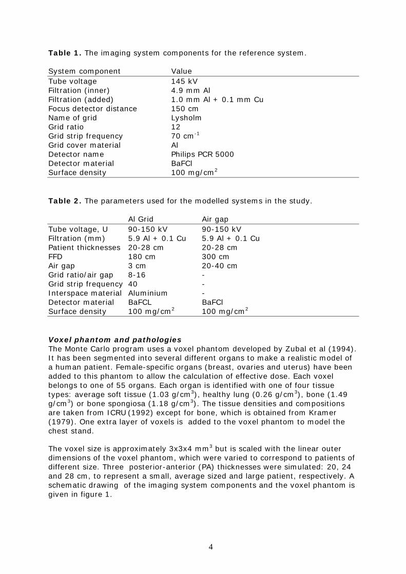
Table 1. The imaging system components for the reference system. System component Value Tube voltage 145 kV Filtration (inner) 4.9 mm Al Filtration (added) 1.0 mm Al + 0.1 mm Cu Focus detector distance 150 cm Name of grid Lysholm Grid ratio 12 Grid strip frequency 70 cm-1 Grid cover material Al Detector name Philips PCR 5000 Detector material BaFCl Surface density 100 mg/cm2 Table 2. The parameters used for the modelled systems in the study. Al Grid Air gap Tube voltage, U 90-150 kV 90-150 kV Filtration (mm) 5.9 Al + 0.1 Cu 5.9 Al + 0.1 Cu Patient thicknesses 20-28 cm 20-28 cm FFD 180 cm 300 cm Air gap 3 cm 20-40 cm Grid ratio/air gap 8-16 - Grid strip frequency 40 - Interspace material Aluminium - Detector material BaFCL BaFCl Surface density 100 mg/cm2 100 mg/cm2 Voxel phantom and pathologies The Monte Carlo program uses a voxel phantom developed by Zubal et al (1994). It has been segmented into several different organs to make a realistic model of a human patient. Female-specific organs (breast, ovaries and uterus) have been added to this phantom to allow the calculation of effective dose. Each voxel belongs to one of 55 organs. Each organ is identified with one of four tissue types: average soft tissue (1.03 g/cm3), healthy lung (0.26 g/cm3), bone (1.49 g/cm3) or bone spongiosa (1.18 g/cm3). The tissue densities and compositions are taken from ICRU (1992) except for bone, which is obtained from Kramer (1979). One extra layer of voxels is added to the voxel phantom to model the chest stand. The voxel size is approximately 3x3x4 mm3 but is scaled with the linear outer dimensions of the voxel phantom, which were varied to correspond to patients of different size. Three posterior-anterior (PA) thicknesses were simulated: 20, 24 and 28 cm, to represent a small, average sized and large patient, respectively. A schematic drawing of the imaging system components and the voxel phantom is given in figure 1.
4

We use six pathological nodules, which are positioned in different regions, corresponding to those used in a clinical trial by Håkansson et al (2004). The diameters of these (spherical) details are chosen so that their object contrast corresponds to the threshold contrast of details determined in the study by Håkansson et al (2004). The chemical compositions of the nodules are taken from Ullman et al (2003) and from references therein. Figure 1. Schematic drawing of the model of the imaging system including the main components of the x-ray unit and a voxel phantom representing the patient.
Figure 2. The regions used in this work, corresponding to the regions in Håkansson et al (2004) (the figure to the right). The regions are A: Apical pulmonary region, B: Lateral pulmonary region, C: Retrocardial region, D: Lower mediastinal region, E: Hilar region, F: Upper mediastinal region.
X-ray tube
Filter
Collimators
Voxel phantom Chest stand
Grid
Cassette-front
Image detector
5
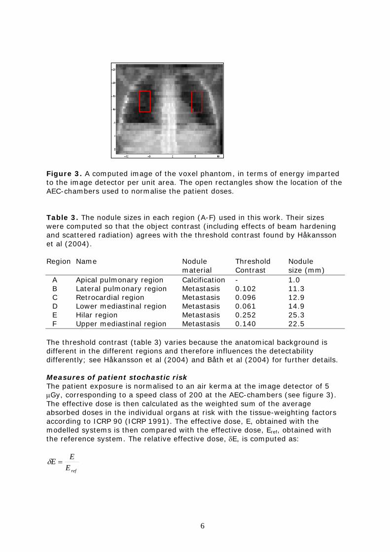
Figure 3. A computed image of the voxel phantom, in terms of energy imparted to the image detector per unit area. The open rectangles show the location of the AEC-chambers used to normalise the patient doses.
Table 3. The nodule sizes in each region (A-F) used in this work. Their sizes were computed so that the object contrast (including effects of beam hardening and scattered radiation) agrees with the threshold contrast found by Håkansson et al (2004). Region Name Nodule Threshold Nodule material Contrast size (mm) A Apical pulmonary region Calcification - 1.0 B Lateral pulmonary region Metastasis 0.102 11.3 C Retrocardial region Metastasis 0.096 12.9 D Lower mediastinal region Metastasis 0.061 14.9 E Hilar region Metastasis 0.252 25.3 F Upper mediastinal region Metastasis 0.140 22.5 The threshold contrast (table 3) varies because the anatomical background is different in the different regions and therefore influences the detectability differently; see Håkansson et al (2004) and Båth et al (2004) for further details. Measures of patient stochastic risk The patient exposure is normalised to an air kerma at the image detector of 5 µGy, corresponding to a speed class of 200 at the AEC-chambers (see figure 3). The effective dose is then calculated as the weighted sum of the average absorbed doses in the individual organs at risk with the tissue-weighting factors according to ICRP 90 (ICRP 1991). The effective dose, E, obtained with the modelled systems is then compared with the effective dose, Eref, obtained with the reference system. The relative effective dose, δE, is computed as:
refEEE =δ
6

Measures of image quality Optimisation is a complex procedure that may be facilitated if physical image quality measures can be found that correlate to the radiologists’ evaluation of the diagnostic information in clinical patient images (Sandborg et al 2001, Tingberg et al 2004, Ullman et al 2004). Here, four ‘figures of merits’ are used to describe physical image quality. These are:
• SNR (ideal observer signal-to-noise ratio) • SNR2/E (dose to information conversion efficiency) • C/Cr (nodule-contrast to rib-contrast ratio • Cdyn (nodule-contrast to image dynamic range ratio)
that are described below. Signal-to-noise, SNR Since the image contrast is readily modified in a digital image, the ideal observer signal-to-noise ratio SNR (ICRU 1996) was used as one measure of image quality. The computer program calculates this SNR for a contrasting detail (nodule) with the area of a pixel, here called the SNRM
2211
2211
sspp
pppp
MNN
NNSNR
εε
εε
′⋅+′⋅
′⋅−′⋅= (1)
where N is the number of photons incident on each pixel. The indices p and s represent contributions from primary and secondary (scattered) photons, respectively. The index n=1 refers to a pixel in the image if the detail is present, and n=2 refers to the same pixel with the detail absent. The quantities ε´ and ε´2 are the mean and mean squared values of the energy imparted per incident photon for the specific pixel. The operator <…> denotes the statistical expectation (mean) value of the specified quantity. From the SNRM it is possible to get the SNR for a given detail as
222DF
pM r
aASNRSNR ⋅⋅= (2)
where A is the projection area of the detail, ap is the pixel area and r2DF is the
signal to noise ratio degradation factor. The latter arises from imaging system unsharpness and additional detector noise and is derived separately according to Sandborg et al (2003). Included in this factor r2 are the geometrical (focal spot- and magnification unsharpness), motion unsharpness and detector unsharpness as described by the pre-sample MTF. The visual transfer function of the human eye-brain system is included in an approximate way. To be able to compare the modelled system with the reference system we define a quantity, δSNR, which is the average of the quotients of the SNR for a given pathology in the modelled system divided by the SNR for the same pathology in the reference system:
∑=q refq
q
SNRSNR
NSNR
,
1δ
7
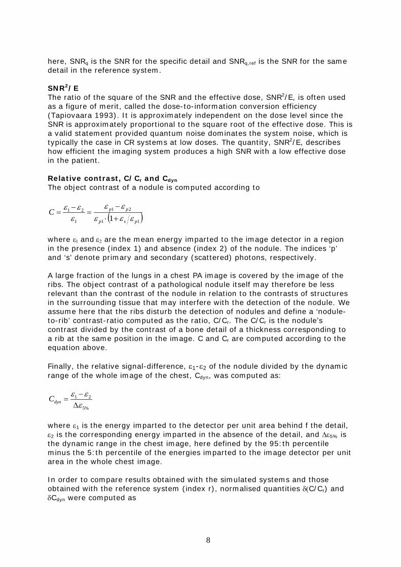
here, SNRq is the SNR for the specific detail and SNRq,ref is the SNR for the same detail in the reference system. SNR2/E The ratio of the square of the SNR and the effective dose, SNR2/E, is often used as a figure of merit, called the dose-to-information conversion efficiency (Tapiovaara 1993). It is approximately independent on the dose level since the SNR is approximately proportional to the square root of the effective dose. This is a valid statement provided quantum noise dominates the system noise, which is typically the case in CR systems at low doses. The quantity, SNR2/E, describes how efficient the imaging system produces a high SNR with a low effective dose in the patient. Relative contrast, C/Cr and Cdyn The object contrast of a nodule is computed according to
( )11
21
1
21
1 psp
ppCεεε
εεε
εε+⋅−
=−
=
where ε1 and ε2 are the mean energy imparted to the image detector in a region in the presence (index 1) and absence (index 2) of the nodule. The indices ‘p’ and ‘s’ denote primary and secondary (scattered) photons, respectively. A large fraction of the lungs in a chest PA image is covered by the image of the ribs. The object contrast of a pathological nodule itself may therefore be less relevant than the contrast of the nodule in relation to the contrasts of structures in the surrounding tissue that may interfere with the detection of the nodule. We assume here that the ribs disturb the detection of nodules and define a ‘nodule-to-rib’ contrast-ratio computed as the ratio, C/Cr. The C/Cr is the nodule’s contrast divided by the contrast of a bone detail of a thickness corresponding to a rib at the same position in the image. C and Cr are computed according to the equation above. Finally, the relative signal-difference, ε1-ε2 of the nodule divided by the dynamic range of the whole image of the chest, Cdyn, was computed as:
%5
21
εεε
∆−
=dynC
where ε1 is the energy imparted to the detector per unit area behind f the detail, ε2 is the corresponding energy imparted in the absence of the detail, and ∆ε5% is the dynamic range in the chest image, here defined by the 95:th percentile minus the 5:th percentile of the energies imparted to the image detector per unit area in the whole chest image. In order to compare results obtained with the simulated systems and those obtained with the reference system (index r), normalised quantities δ(C/Cr) and δCdyn were computed as
8

( ) ∑=q refrqq
rqqr CC
CCN
CC,,
,1δ
∑ ∆∆
=q refrefq
qdyn C
CN
Cεε
δ,
1
The summation is over q=N nodules in the image. Results The computations were completed for three patient AP-dimensions, 20, 24 and 28 cm and are presented in a group of three subsequent figures, representing each patient size.
Effective dose Figures 4-6 show the effective dose and the entrance air kerma without backscatter, Kc,air, for 20-28 cm thick patients. The effective dose for fixed AEC-setting is fairly constant with varying tube voltage using the air gap technique, but increases with increasing air gap length. With the grid technique, E, increases with increasing grid ratio and also increases slowly with decreasing tube voltage. The effective dose is generally lower using the air gap technique compared to the grid technique, particularly at lower tube voltages and higher grid ratios due to increased attenuation of primary and secondary (scattered) photons in the grid. The dose-advantage of the air gap technique is between 25-70% for an average sized patient (24 cm PA thickness). The effective dose for a 20 cm thick patient is 25% larger at 150 kV for the grid with ratio 8 compared to using a 20 cm air gap at the same tube voltage. For the same patient thickness and tube voltage, using a grid with ratio 16 would give 67% larger dose compared with a 20 cm air gap. The effective dose increases approximately 50% when the patient PA-thickness increases from 20 cm to 28 cm. The figures also show the variation of the incident air kerma without backscatter, Kc,air, with increasing grid ratio, air gap length and tube voltage. The same general trend is found as for the effective dose, except that the variation with tube voltage is stronger, resulting in comparably lower air kerma at high tube voltages. This is mainly due to the increase of the conversion factor E/ Kc,air, with increasing tube voltage (see for example Hart et al 1994).
Figures of merit SNR The variation of SNR with imaging parameters are given in figures 7-15. In the apical pulmonary region (A), the SNR increases rapidly (60-70%) with decreasing tube voltage (90-150 kV). It is approximately 20% higher with the air gap compared to the grid technique and decreases with 20% when the patient thickness increases from 20 cm to 28 cm. In the laterally pulmonary (B) and hilar (E) regions there is a 30-40% increase in SNR with decreasing tube voltage. The increase is larger with the grid technique
9

than with the air gap technique. There is a small (10-20%) SNR-advantage of using the air gap compared to the grid technique. As expected the SNR decreases with increasing patient thickness. Similar trends are observed in the retrocardial (C) and lower (D) and upper (F) mediastinal regions, except that the SNR advantage of the air gap technique is smaller. In the mediastinal regions there is, contrary to in the other regions, a significant SNR-advantage with using a grid with a high ratio (16) over the air gap lengths used in this study. SNR2/E The variation of SNR2/E with imaging parameters are given in figures 16-24. In all regions the SNR2/E decreases with increasing tube voltage. The decrease is more rapid in the apical region (A) since the nodule (calcification) contains materials with higher atomic numbers than the soft tissue nodules in the other five regions (B-F). In the apical, lateral, and hilar pulmonary regions as well as in the retrocardial pulmonary regions (i.e. the less dense regions) for thin patients, the SNR2/E is only slowly depending on the grid ratio and air gap length. In regions with more tissue material in the primary beam, such as the upper- and lower mediastinal regions and in the retrocardial pulmonary regions for thicker patients, SNR2/E increases more rapidly with increasing grid ratio and air gap length. The rate of increase of the SNR2/E with increasing grid ratio is larger for thicker patients than for thin patients and is also larger at lower tube voltages. In the less dense regions, the air gap technique provides a higher SNR2/E than the grid technique, at equal tube voltage, even when the largest grid ratio (r=16) is used. However in the densest upper- and lower mediastinal regions for thickest patients, the use of the highest grid ratio (r=16) provides a slightly higher SNR2/E than with the air gap technique. Nodule to rib contrast-ratio, C/Cr The variation of C/Cr with imaging parameters are given in figures 25-33. The ratio, C/Cr, is independent of grid ratio, air gap length and patient thickness. In the apical and laterally pulmonary regions, it is also constant with tube voltage. In the other regions (C-F), C/Cr increases approximately 10-20% with increasing tube voltage providing a comparably higher contrast of the soft tissue nodule compare to the overlaying ribs. Both the contrast of the metastasis nodule and the rib decreases with increasing tube voltage but the rate of decrease is larger for the bony structure (rib) due to a more pronounced influence of the photoelectric effect on the contrast for details with higher atomic number. Contrast relative to the dynamic range, Cdyn The variation of Cdyn with imaging parameters are given in figures 34-42. In the apical region (A), Cdyn decreases 30-40% with increasing tube voltage, indicating better performance for detecting the calcification at lower tube voltages. The values are 20-25% higher with the air gap technique compared to the grids, again giving the air gap technique an advantage over the grids.
10
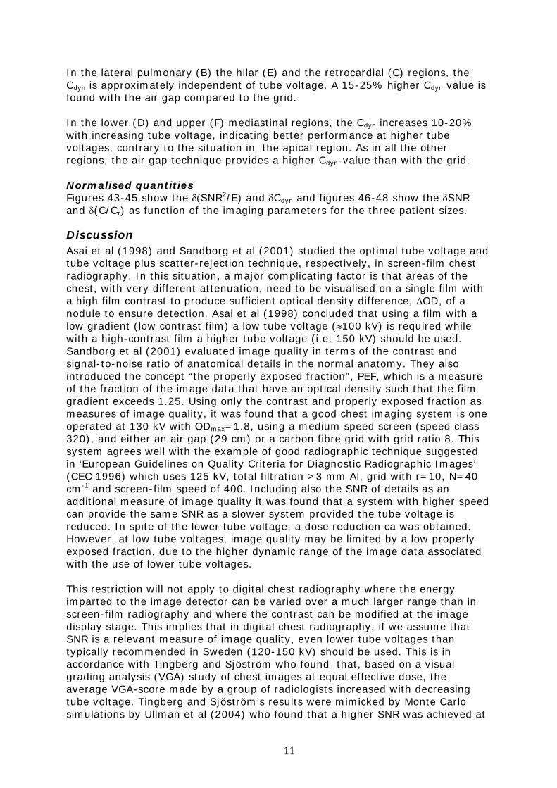
In the lateral pulmonary (B) the hilar (E) and the retrocardial (C) regions, the Cdyn is approximately independent of tube voltage. A 15-25% higher Cdyn value is found with the air gap compared to the grid. In the lower (D) and upper (F) mediastinal regions, the Cdyn increases 10-20% with increasing tube voltage, indicating better performance at higher tube voltages, contrary to the situation in the apical region. As in all the other regions, the air gap technique provides a higher Cdyn-value than with the grid. Normalised quantities Figures 43-45 show the δ(SNR2/E) and δCdyn and figures 46-48 show the δSNR and δ(C/Cr) as function of the imaging parameters for the three patient sizes.
Discussion Asai et al (1998) and Sandborg et al (2001) studied the optimal tube voltage and tube voltage plus scatter-rejection technique, respectively, in screen-film chest radiography. In this situation, a major complicating factor is that areas of the chest, with very different attenuation, need to be visualised on a single film with a high film contrast to produce sufficient optical density difference, ∆OD, of a nodule to ensure detection. Asai et al (1998) concluded that using a film with a low gradient (low contrast film) a low tube voltage (≈100 kV) is required while with a high-contrast film a higher tube voltage (i.e. 150 kV) should be used. Sandborg et al (2001) evaluated image quality in terms of the contrast and signal-to-noise ratio of anatomical details in the normal anatomy. They also introduced the concept “the properly exposed fraction”, PEF, which is a measure of the fraction of the image data that have an optical density such that the film gradient exceeds 1.25. Using only the contrast and properly exposed fraction as measures of image quality, it was found that a good chest imaging system is one operated at 130 kV with ODmax=1.8, using a medium speed screen (speed class 320), and either an air gap (29 cm) or a carbon fibre grid with grid ratio 8. This system agrees well with the example of good radiographic technique suggested in ‘European Guidelines on Quality Criteria for Diagnostic Radiographic Images’ (CEC 1996) which uses 125 kV, total filtration >3 mm Al, grid with r=10, N=40 cm-1 and screen-film speed of 400. Including also the SNR of details as an additional measure of image quality it was found that a system with higher speed can provide the same SNR as a slower system provided the tube voltage is reduced. In spite of the lower tube voltage, a dose reduction ca was obtained. However, at low tube voltages, image quality may be limited by a low properly exposed fraction, due to the higher dynamic range of the image data associated with the use of lower tube voltages. This restriction will not apply to digital chest radiography where the energy imparted to the image detector can be varied over a much larger range than in screen-film radiography and where the contrast can be modified at the image display stage. This implies that in digital chest radiography, if we assume that SNR is a relevant measure of image quality, even lower tube voltages than typically recommended in Sweden (120-150 kV) should be used. This is in accordance with Tingberg and Sjöström who found that, based on a visual grading analysis (VGA) study of chest images at equal effective dose, the average VGA-score made by a group of radiologists increased with decreasing tube voltage. Tingberg and Sjöström’s results were mimicked by Monte Carlo simulations by Ullman et al (2004) who found that a higher SNR was achieved at
11

tube voltages below 100 kV than at tube voltages above 125 kV. Dobbins et al (1992) also concluded that with CR digital radiography, detection was superior at 100 kV compared to at 140 kV Chotas et al (1993) studied a CR system (ST III plates) in bedside chest AP radiography at equal effective dose and concluded that using 60 kV compared to typically 120 kV resulted in a 15% higher SNR in the lung regions. The SNR in the mediastinum and subdiaphragm regions were not significantly affected by the change in tube voltage. They expected that the SNR-advantage of using lower tube voltage to be even higher in the PA projection (which is the standard projection for erect patients). They further argue that even if image SNR cannot perfectly predict observer performance in any diagnostic task, it is reasonable to assume that trends in SNR will be matched by trends in detectability performance, as SNR is a primary determiner of perceptibility in an image. Launders et al (2001) investigated the optimal tube voltage with a Thoravision digital detector that uses an air gap for scatter-rejection. They found a minimum in effective dose at 90-110 kV, and concluded that image quality decreases with increasing tube voltage. This is in agreement with Sandborg et al (2001) in their evaluation of a 29 cm air gap technique in screen-film chest radiography. Launders et al (2001) also claim that objective measurements can be used to optimise radiographic technique without prolonged patient trials. This contradicts the conclusions by Håkansson et al (2004), which are discussed below. Håkansson et al (2004) explored how the value of the threshold contrast depends on the location of a 10 mm nodule in the chest PA image and the relative influence of different sources of noise; system quantum noise, anatomical noise and anatomical background structures. The latter factor is not noise in the common sense but merely variability (‘busyness’) of the background in the chest region that may interfere with the radiologist’s detection of nodules in the lungs. The trend found by Håkansson et al (2004) was that in the hilar region, a significantly higher threshold contrast was needed for accurate detection compared to in the lateral pulmonary and retrocardial regions. Implications of this is found in table 3 where the size of the nodule (Ullman et al 2004) required to result in the threshold contrast found by Håkansson et al (2004) is over twice as large in the hilar region as in the retrocardial region. Their study imply that quantum noise is not limiting the observers detection of the nodules, but instead the anatomical background structures, which are of major concern, particularly, in the hilar region. If anatomical background structures is the most important factor influencing the detection of nodules in the chest PA radiograph, i.e. more important than system quantum noise, then it is important to identify such structures and to reduce their negative influence on detection of pathological structures (i.e. metastasis nodules). One way to quantify the perception of the pathological nodules in relative to the anatomical background is to compute the contrast ratio, C/Cr. This study shows that in most regions in the chest (C-F) this contrast-ratio increases with increasing tube voltage indicating that the contrast of the metastasis nodule is enhanced compared to the contrast of the ribs, here interpreted as an anatomical background structure. This is in agreement with Samei (2004) who also pointed out the importance of reducing the relative contrast of the ribs. Fransson (2004) however, also argued that in some cases it is also important to
12

see the ribs clearly in order to detect possible lesions in them. ICRU (2003) and references therein, discuss various other factors influencing the selection of tube voltage and scatter-rejection technique. Sandborg et al (1993 and 1994) studied the selection of tube voltage and scatter-rejection technique in screen-film and digital chest radiography with a simple (water-box) model of the patient. In examinations with relatively small amounts of scatter, the air gap technique was advantageous but it needs to be used in combination of lower tube voltages to achieve the same contrast as with the grid. The optimal tube voltage was defined as the one that minimises the mean absorbed dose in the phantom for a fixed SNR. In chest frontal view, the optimal tube voltage was approximately 80 kV. The minimum was very shallow and the mean absorbed dose was only 25% higher at 120 kV compared to at 80 kV. In the figures for the SNR2/E, all show a decreasing SNR2/E with increasing tube voltage. This would suggest that the tube voltage could be lowered from the conventional range of 120-150 kV down to 90 kV to produce images with lower noise. However, in the figures concerning the nodule-to-rib contrast, C/Cr and the Cdyn, the relation is the opposite, with the figures of merit increasing with increasing tube voltages. This is valid in all regions except in the apical pulmonary region, where a calcification detail is used. Maintaining the current dose level, where the quantum noise is low enough not to limit the radiologist’s performance, would suggest using high tube voltages if the diagnostic task is to detect metastasis nodules in the lungs. If, on the other hand, the diagnostic task is detection of calcifications, use of low tube voltages in the range of 90 kV should be recommended.
Conclusions In all regions, but in the densest regions in the thickest patients, the air gap technique provides higher SNR and object contrast than the grid technique and at a lower patient dose, yielding a significantly higher SNR2/E with the air gap. The selection of tube voltage is less straightforward. The figures of merit SNR and SNR2/E, indicate that lower tube voltages should be selected since higher values are obtained for nodules using lower tube voltages. On the other hand, the C/Cr nodule-to-rib contrast-ratio increases with increasing tube voltage, indicating that the relative contrast of soft tissue compared to bone increases with increasing tube voltage. If anatomical background structures (such as ribs) are believed to interfere with the radiologist’s detection of low-contrast soft-tissue details, higher tube voltages should be preferred as the contrast of the nodules increases compared to the contrast of the ribs as the tube voltage increases.
Acknowledgement This report was completed under the 5th framework program contract number FIGM-CT-2000-00036.
13

References Y. Asai, Y. Tanabe, Y. Ozaki, H. Kubota, and M. Matsumoto. Optimum tube voltage for chest radiographs obtained by psychophysical analysis, Med. Phys. 25, 2170-2175, 1998. M. J. Berger and J. H. Hubbell. XCOM: Photon Cross Section on a Personal Computer, NBSIR 87-3597, U.S. Department of Commerce, National Bureau of Standards, Office of Standard Reference Data, Gaithersburg MD 20899 (1987). R. Birch, B. Marshall and G. M. Ardran. Catalogue of spectral data for diagnostic X-rays, The Hospital Physicists' Association, Scientific Report Series 30, 47 Belgrave Square (London, 1979). Båth M, Börjesson S, Håkansson H, Kheddache S, Grahn A, Bochud FO, Verdun FR and Månsson LG. Nodule detection in digital chest radiography: part of image background acting as pure noise. (Submitted to Rad Prot Dosim) Båth M, Börjesson S, Håkansson M, Hoeschen C, Tischenko O, Kheddache S, Vikgren J and Månsson LG. Nodule detection in digital chest radiography: effect of anatomical noise. (Submitted to Rad Prot Dosim 2004). CEC 1996. European Guidelines on Quality Criteria for Diagnostic Radiographic Images, EUR 16260 EN, ISBN 92-827-7284-5, (Luxembourg Office for publication of the European Communities; 1996) H G Chotas, C F Floyd, J T Dobbins 3rd, CE Ravlin. Digital chest radiography with photostimuable storage phosphors: signal-to-noise ratio as a function of kilovoltage with matched exposure risk Radiology 186, 395-398, 1993. D R Dance, S A Lester, G Alm Carlsson, M Sandborg and J Persliden. The use of fibre material in radiographic cassettes: estimation of the dose and contrast advantages British Journal of Radiology 70, 383-390, 1997. J T Dobbins 3rd, J J Rice, C A Beam, C E Ravin. Threshold perception performance with computed and screen-film radiography: Implications for chest radiography, Radiology, 183, 179-187, 1992. S-G Fransson. (Private communication 2004, Chest Radiologist, Thoracic Radiology Department, Linköping University Hospital) ICRP, 1990 Recommendations of the International Commission on Radiological Protection. Annals of the ICRP, publication 60 (Pergamon Press, Oxford, 1991). ICRU, Photon, electron, proton, and neutron interaction data for body tissues, Report No. 46 International Commission on Radiation Units and Measurements (Bethesda, USA, 1992). ICRU, Medical Imaging - The Assessment of Image Quality. ICRU Report 54 International Commission on Radiation Units and Measurements (Bethesda, USA, 1996). J H Launders, A R Cowen, R F Bury, P Hawkridge. Towards image quality, beam energy and effective dose optimisation in digital thoracic radiography. Eur. Radiol., 11, 870-875, 2001. ICRU. Image quality in chest radiography. Journal of the ICRU ISSN 1473-6691, Vol 3 no 2 (Nuclear Technology Publishing, 2003)
14

M Håkansson, M Båth, S Börjesson, S Khedache, G Ullman, L-G Månsson. Nodule detection in digital chest radiography: effect of nodule location (Submitted to Rad Prot Dosim) D Hart, DG Jones, BF Wall. Estimation of effective dose in diagnostic radiology from entrance surface dose and dose-area product measurements NRPB-R262 Chilton: National Radiological Protection Board, 1994. J. H. Hubbell and I. Överbö. Relativistic atomic form factors and photon coherent scattering cross section, J. Phys. Chem. Ref. Data 8, 69-105 (1979). J. H. Hubbell, Wm. J. Veigele, E. A. Briggs, R. T. Brown, D. T. Cromer and R. J. Howerton. Atomic form factors, incoherent scattering functions and photon scattering cross sections, J. Phys. Chem. Ref. Data 4, 471-538, 1975. R. Kramer. Determination of conversion factors between body dose and relevant radiation quantities for external x-and γ radiation, GSF Bericht-S-556 (GSF, Neuherberg, Germany, 1979). G McVey, M Sandborg, D R Dance, and G Alm Carlsson. A study and optimisation of lumbar spine x-ray imaging systems Br J Radiol 76: 177-188, 2003. E. Samei (Private communication, Malmö Congress on Medical Imaging April 2004) Sandborg M, Dance DR, Alm Carlsson G, Persliden J and Tapiovaara M J. Monte Carlo study of grid performance in diagnostic radiology: task dependent optimisation for digital imaging. Phys Med Biol. 39, 1659-1676, 1994. Sandborg M, Dance D R, Alm Carlsson G and Persliden J. Monte Carlo study of grid performance in diagnostic radiology; factors which affect the selection of tube potential and grid ratio. Brit J Radiol 66, 1164-1176, 1993. M. Sandborg, G. McVey, D.R. Dance and G. Alm Carlsson. Schemes for the optimization of chest radiography using a computer model of the patient and x-ray imaging system. Medical Physics 28 2007-2019, 2001. Sandborg M, Dance D R, Alm Carlsson G and Persliden J Selection of antiscatter grids for different imaging tasks: the advantage of low atomic number cover and interspace materials. Brit J Radiol 66, 1151-1163, 1993. M Sandborg, D R Dance and G Alm Carlsson. Calculation of contrast and signal-to-noise degradation factors for digital detectors in chest and breast imaging ISRN ULI-RAD-R-93—SE, 2003. M Sandborg, A Tingberg, D R Dance, B Lanhede, A Almén, G McVey, P Sund, S Kheddache, J Besjakov, S Mattsson, L G Månsson, and G Alm Carlsson. Demonstration of correlations between clinical and physical image quality measures in chest and lumbar spine screen-film radiography British Journal of Radiology 74, 520-528, 2001. M J Tapiovaara. SNR and noise measurement for medical imaging: II. Application to fluoroscopy x-ray equipment. Med Phys, 38, 1761-1788, 1993. A Tingberg, M Båth, M Håkansson, J Medin, M Sandborg, G Alm Carlsson, S Mattsson and L G Månsson. Comparison of two methods for evaluation of image quality of lumbar spine radiographs SPIE vol 5372, 2004.
15

G Ullman, M Sandborg and G Alm Carlsson. Validation of a voxel-phantom based Monte Carlo model and calibration of digital systems. ISRN ULI-RAD-R-95—SE, 2003. I. G. Zubal, C. R. Harrell, E. O. Smith, Z. Rattner, G. Gindi and P. B. Hoffer. Computerized three-dimensional segmented human anatomy, Med Phys. 299-302, 1994.
16

Figure 4. The effective dose and entrance air kerma for a 20 cm thick patient17

Figure 5. The effective dose and entrance air kerma for a 24 cm thick patient18

Figure 6. The effective dose and entrance air kerma for a 28 cm thick patient19

Figure 7. The SNR in the apical and lateral pulmonary regions for a 20 cm thick patient
20

Figure 8. The SNR in the apical and lateral pulmonary regions for a 24 cm thick patient
21

Figure 9. The SNR in the apical and lateral pulmonary regions for a 28 cm thick patient
22

Figure 10. The SNR in the hilar and lower mediastinal regions for a 20 cm thick patient
23

Figure 11. The SNR in the hilar and lower mediastinal regions for a 24 cm thick patient
24

Figure 12. The SNR in the hilar and lower mediastinal regions for a 28 cm thick patient
25

Figure 13. The SNR in the retrocardial and upper mediastinal regions for a 20 cm thick patient
26

Figure 14. The SNR in the retrocardial and upper mediastinal regions for a 24 cm thick patient
27
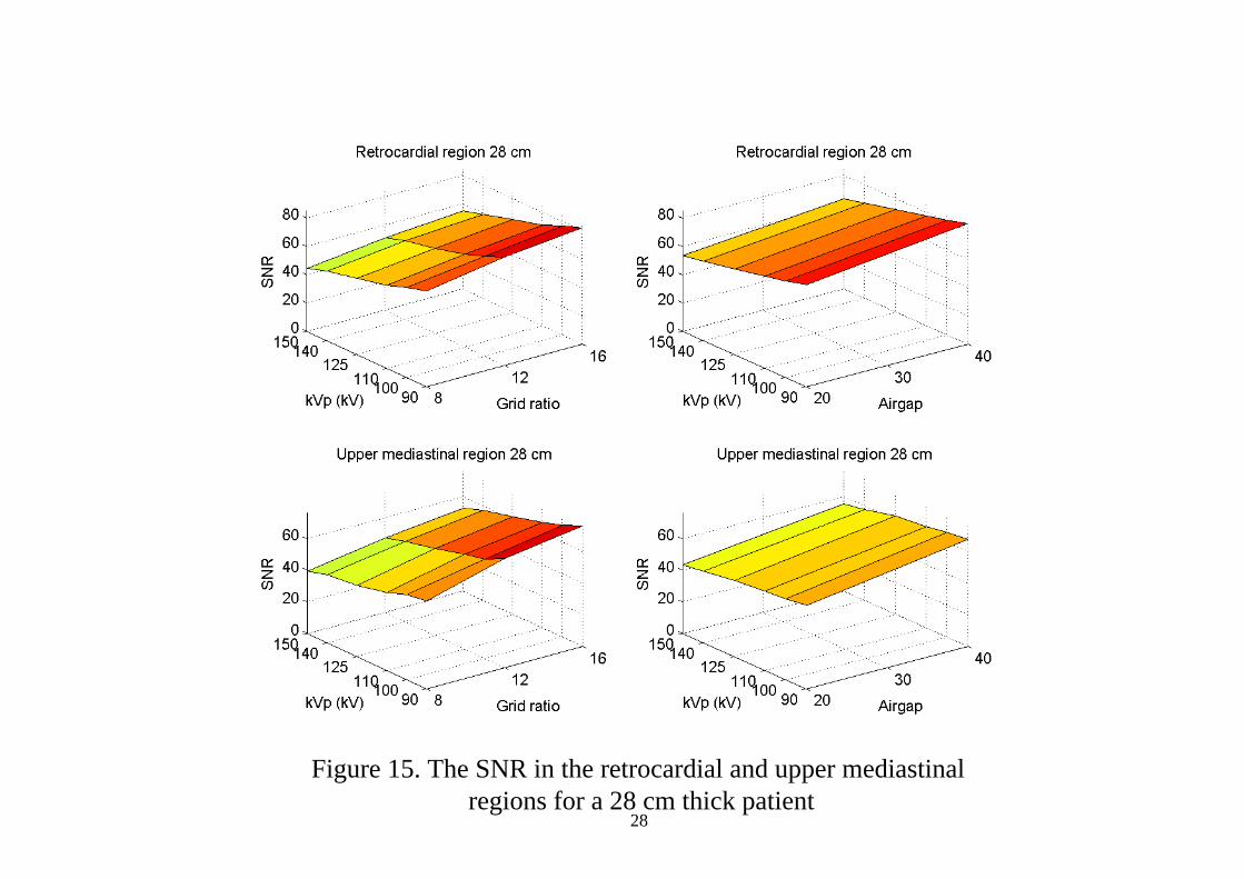
Figure 15. The SNR in the retrocardial and upper mediastinal regions for a 28 cm thick patient
28

Figure 16. The SNR2/E in the apical and lateral pulmonary regions for a 20 cm thick patient
29

Figure 17. The SNR2/E in the apical and lateral pulmonary regions for a 24 cm thick patient
30

Figure 18. The SNR2/E in the apical and lateral pulmonary regions for a 28 cm thick patient
31

Figure 19. The SNR2/E in the hilar and lower mediastinal regions for a 20 cm thick patient
32

Figure 20. The SNR2/E in the hilar and lower mediastinal regions for a 24 cm thick patient
33

Figure 21. The SNR2/E in the hilar and lower mediastinal regions for a 28 cm thick patient
34

Figure 22. The SNR2/E in the retrocardial and upper mediastinal regions for a 20 cm thick patient
35

Figure 23. The SNR2/E in the retrocardial and upper mediastinal regions for a 24 cm thick patient
36

Figure 24. The SNR2/E in the retrocardial and upper mediastinal regions for a 28 cm thick patient
37

Figure 25. The C/Cr in the apical and lateral pulmonary regions for a 20 cm thick patient
38

Figure 26. The C/Cr in the apical and lateral pulmonary regions for a 24 cm thick patient
39

Figure 27. The C/Cr in the apical and lateral pulmonary regions for a 28 cm thick patient
40
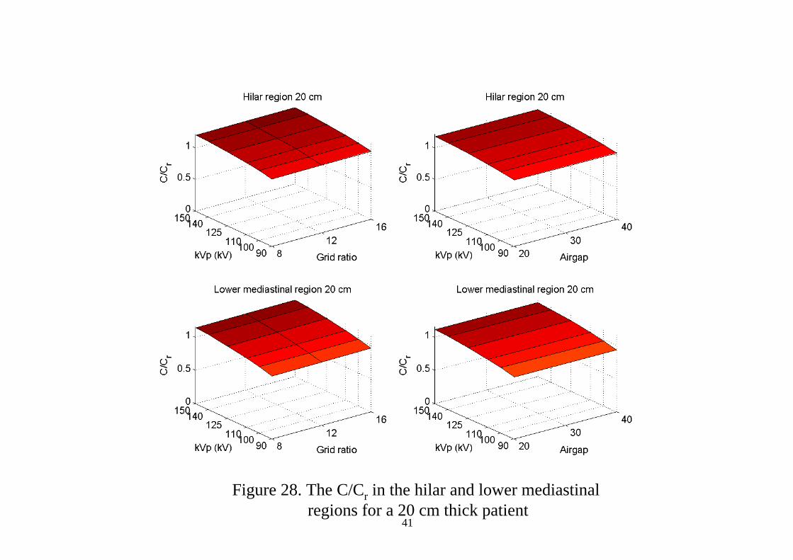
Figure 28. The C/Cr in the hilar and lower mediastinal regions for a 20 cm thick patient
41

Figure 29. The C/Cr in the hilar and lower mediastinal regions for a 24 cm thick patient
42

Figure 30. The C/Cr in the hilar and lower mediastinal regions for a 28 cm thick patient
43

Figure 31. The C/Cr in the retrocardial and upper mediastinal regions for a 20 cm thick patient
44

Figure 32. The C/Cr in the retrocardial and upper mediastinal regions for a 24 cm thick patient
45

Figure 33. The C/Cr in the retrocardial and upper mediastinal regions for a 28 cm thick patient
46
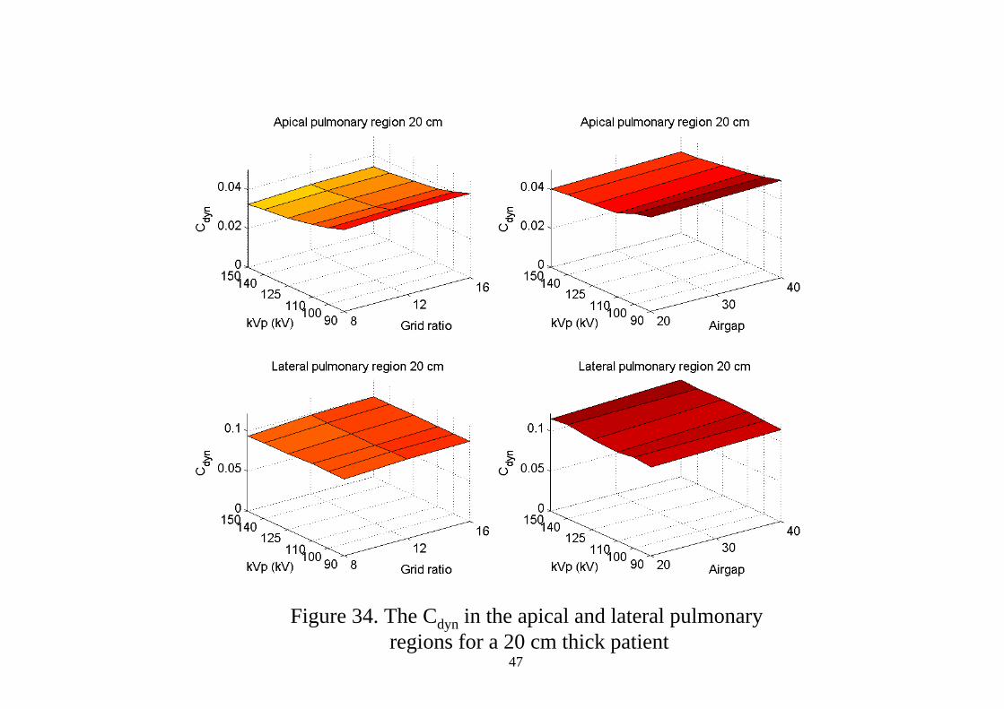
Figure 34. The Cdyn in the apical and lateral pulmonary regions for a 20 cm thick patient
47

Figure 35. The Cdyn in the apical and lateral pulmonary regions for a 24 cm thick patient
48
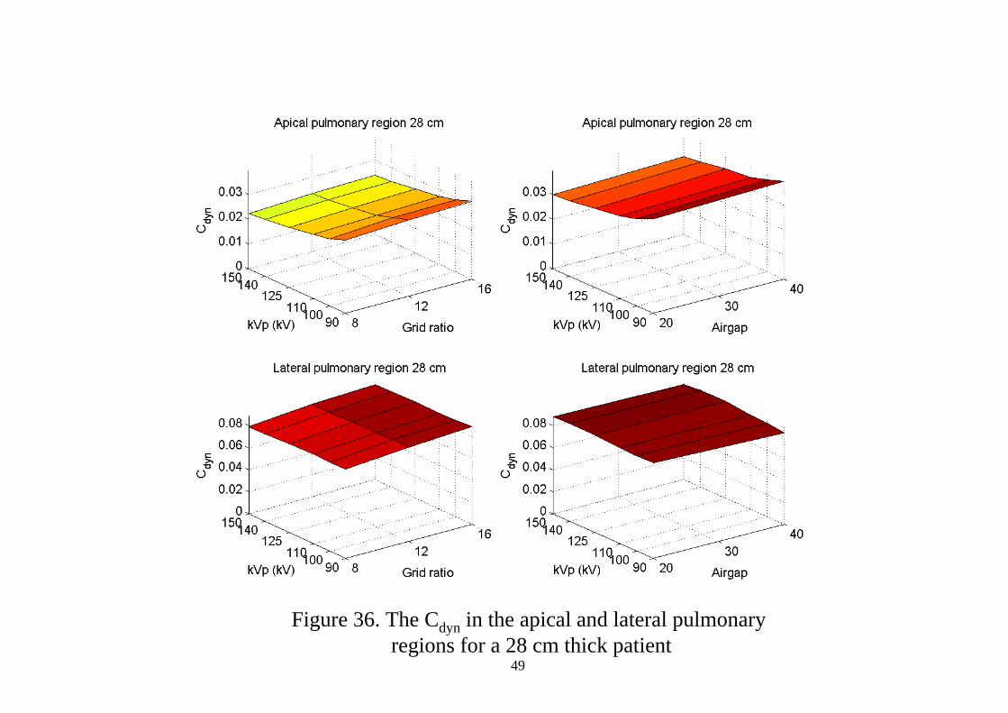
Figure 36. The Cdyn in the apical and lateral pulmonary regions for a 28 cm thick patient
49

Figure 37. The Cdyn in the hilar and lower mediastinal regions for a 20 cm thick patient
50

Figure 38. The Cdyn in the hilar and lower mediastinal regions for a 24 cm thick patient
51
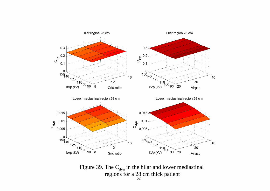
Figure 39. The Cdyn in the hilar and lower mediastinal regions for a 28 cm thick patient
52

Figure 40. The Cdyn in the retrocardial and upper mediastinal regions for a 20 cm thick patient
53
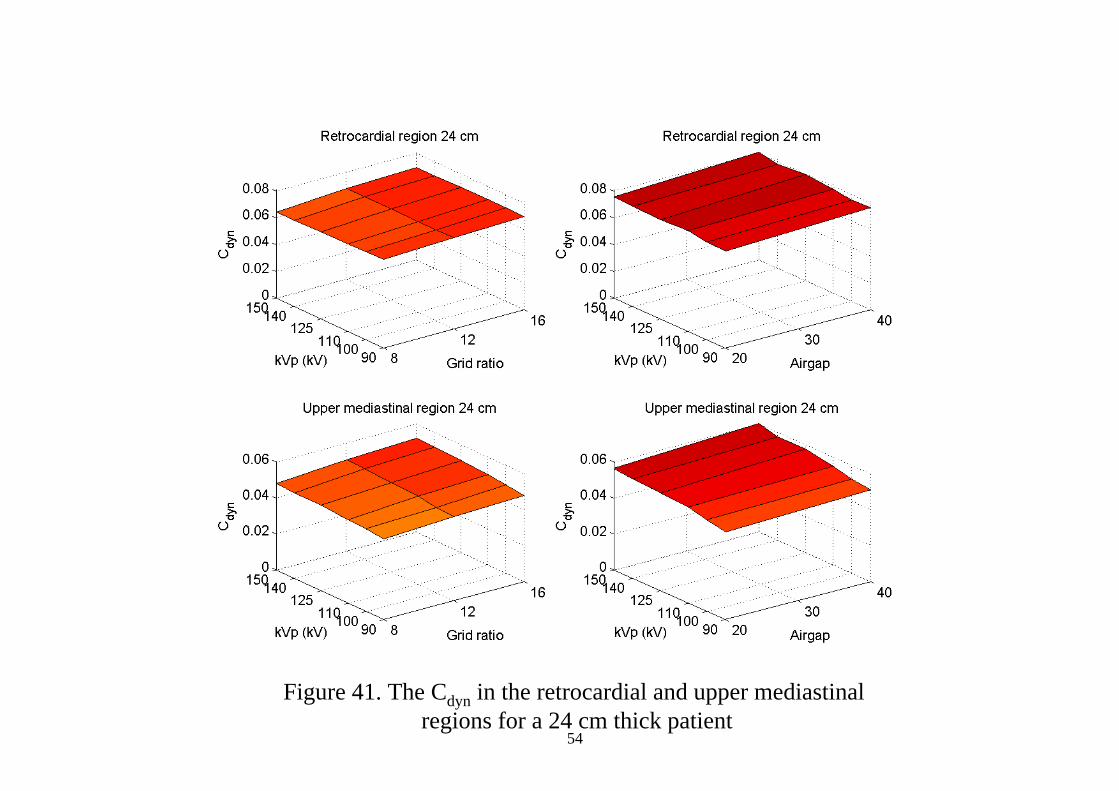
Figure 41. The Cdyn in the retrocardial and upper mediastinal regions for a 24 cm thick patient
54

Figure 42. The Cdyn in the retrocardial and upper mediastinal regions for a 28 cm thick patient
55

Figure 43. The δSNR2/δE and δCdyn for a 20 cm thick patient56

Figure 44. The δSNR2/δE and δCdyn for a 24 cm thick patient57

Figure 45. The δSNR2/δE and δCdyn for a 28 cm thick patient58

Figure 46. The δSNR and δC/δCr for a 20 cm thick patient59
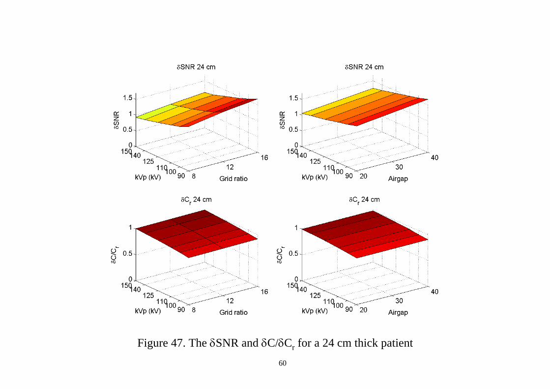
Figure 47. The δSNR and δC/δCr for a 24 cm thick patient60

Figure 48. The δSNR and δC/δCr for a 28 cm thick patient61