Optimisation of a non-linear tuned vibration absorber in a...

Optimisation of a non-linear tuned vibrationabsorber in a hand-held impact machine

Master’s Thesis in Applied Mechanics

MATTIAS JOSEFSSONSNÆVAR LEO GRETARSSON

Department of Applied MechanicsCHALMERS UNIVERSITY OF TECHNOLOGYGoteborg, Sweden 2015

MASTER’S THESIS IN APPLIED MECHANICS

Optimisation of a non-linear tuned vibration absorber in a hand-held

impact machine

MATTIAS JOSEFSSONSNÆVAR LEO GRETARSSON

Department of Applied MechanicsDivision of Dynamics

CHALMERS UNIVERSITY OF TECHNOLOGY

Goteborg, Sweden 2015

Optimisation of a non-linear tuned vibration absorber in a hand-held impact machineMATTIAS JOSEFSSONSNÆVAR LEO GRETARSSON

c© MATTIAS JOSEFSSON, SNÆVAR LEO GRETARSSON, 2015

Master’s Thesis 2015:19ISSN 1652-8557Department of Applied MechanicsDivision of DynamicsChalmers University of TechnologySE-412 96 GoteborgSwedenTelephone: +46 (0)31-772 1000

Cover:Previous pneumatic breaker prototype made by Swerea IVF, standing in a stone in Avja quarry. In thebackground is one of the older machines without any vibration reduction.

Chalmers ReproserviceGoteborg, Sweden 2015

Optimisation of a non-linear tuned vibration absorber in a hand-held impact machineMaster’s Thesis in Applied MechanicsMATTIAS JOSEFSSONSNÆVAR LEO GRETARSSONDepartment of Applied MechanicsDivision of DynamicsChalmers University of Technology

Abstract

Traditionally, hand-held impact machines (HHIM) such as pneumatic breakers have little or no means ofvibration reduction. Consequently, vibration injuries are a common problem for individuals working with themon a daily basis. Some existing HHIM utilise vibration isolation between the handle and the impact mechanism,but the vibrations are still above the levels defined by health standards.

Swerea IVF is currently running a project with the long-term goal to prevent all vibration injuries in industry. Abreakthrough towards that goal was to successfully implement a non-linear tuned vibration absorber (TVA) ona pneumatic HHIM prototype and thereby lowering the vibrations significantly on a wide frequency band. Someelectric machines have previously been fitted with a TVA but the varying operating frequency of pneumaticmachines has been a problem since traditional linear TVAs are only effective in a very narrow frequency range.

This thesis investigates how the new non-linear TVA parameters can be optimised to minimise the vibrations ofthe prototype while keeping the suppression band wide enough. An efficient, verified and validated simulationmodel of a pneumatic breaker utilising a non-linear TVA is developed and implemented in Matlab. The modelis used to optimise the 3 parameters of the TVA and to investigate the sensitivity of the solution to differentmodel parameters. It is also investigated how the mass ratio of the TVA affects the optimal solution. Theresults show that using a non-linear TVA can significantly reduce the vibration of a pneumatic HHIM over abroad frequency range and thereby reduce the risk of vibration injuries significantly.

Keywords: Impact machine, Non-linear, Tuned vibration absorber, Tuned mass damper, Multi-body simulation,Hand-arm vibration

, Applied Mechanics, Master’s Thesis, 2015:19 V

Preface

This thesis work is submitted as the final requirement for our MSc degrees in Applied Mechanics from ChalmersUniversity of Technology. The work was carried out during a period of 20 weeks, from January to June 2015.It was conducted on behalf of and in close cooperation with Swerea IVF, a Swedish research institute withinproduction and product development. Hans Lindell was our supervisor at IVF and Professor Viktor Berbyukwas our examiner at Chalmers.

Acknowledgements

There are two people we would like to thank for the opportunity to be part of this exciting work and forgreat help along the way to successfully finishing this thesis. Our first thanks goes to our examiner ViktorBerbyuk, for his good feedback, ideas and endless help. Secondly, we are truly grateful to Hans Lindell, oursupervisor at Swerea IVF, for consistently being there with insightful thoughts and unsurpassed enthusiasm forthis technology and engineering thinking in general. Many thanks to both of you.

Goteborg, June 2015

Mattias Josefsson Snævar Leo Gretarsson

, Applied Mechanics, Master’s Thesis, 2015:19 VII

Nomenclature

Symbol Unit Descriptionmm kg Main massma kg Auxiliary massmh kg Housing massmpist kg Piston masskm N/m Stiffness between main mass and groundka N/m Stiffness between main mass and auxiliary masskh N/m Stiffness between main mass and housingkp N/m Hand-arm stiffness between housing and groundcm N s/m Damping between main mass and groundca N s/m Damping between main mass and auxiliary massch N s/m Damping between main mass and housingcp N s/m Hand-arm damping between housing and grounda m Gap of auxiliary springF0 N Preload of auxiliary springb m Compression length of auxiliary springFe N Exciting force from piston acting on main mass|Fe| N Amplitude of exciting forceFk N Non-linear auxiliary spring force acting on main massx1, x2, x3 m Displacements of main mass, auxiliary mass and housing respectivelyxrel m Auxiliary mass displacement relative the main mass; x2 − x1z(t) State vector as a function of timeP Set of parametersP0 Set of parameters, nominal valuesp Set of normalised parameterspx Normalised parameter x, where x is any of the model parametersf Hz Operating frequency (or excitation frequency)fnom Hz Nominal operating frequencyfres Hz Resonance frequency of non-linear auxiliary systemW (f) Weighting as a function of frequencyL Objective function value

Abbrevations

Abbrevation DescriptionTVA Tuned Vibration AbsorberLTVA Linear Tuned Vibration AbsorberNLTVA Non-Linear Tuned Vibration AbsorberHAVS Hand-Arm Vibration SyndromeHHIM Hand-Held Impact MachineDOF Degree Of FreedomRMS Root Mean SquareODE Ordinary Differential EquationFFT Fast Fourier Transform

, Applied Mechanics, Master’s Thesis, 2015:19 IX

Contents

Abstract V

Preface VII

Acknowledgements VII

Nomenclature IX

Abbrevations IX

Contents XI

1 Introduction 11.1 Background . . . . . . . . . . . . . . . . . . . . . . . . . . . . . . . . . . . . . . . . . . . . . 11.2 Purpose . . . . . . . . . . . . . . . . . . . . . . . . . . . . . . . . . . . . . . . . . . . . . . . 11.3 Limitations . . . . . . . . . . . . . . . . . . . . . . . . . . . . . . . . . . . . . . . . . . . . . 2

2 Theory and method 22.1 Tuned vibration absorbers . . . . . . . . . . . . . . . . . . . . . . . . . . . . . . . . . . . . . 22.2 Hand-arm vibration . . . . . . . . . . . . . . . . . . . . . . . . . . . . . . . . . . . . . . . . . 42.3 The prototype machine . . . . . . . . . . . . . . . . . . . . . . . . . . . . . . . . . . . . . . . 52.4 Analytical formulas for the auxiliary system . . . . . . . . . . . . . . . . . . . . . . . . . . . . 72.5 Measurements . . . . . . . . . . . . . . . . . . . . . . . . . . . . . . . . . . . . . . . . . . . . 72.6 Computations . . . . . . . . . . . . . . . . . . . . . . . . . . . . . . . . . . . . . . . . . . . . 8

3 The model 83.1 Non-linear tuned vibration absorber . . . . . . . . . . . . . . . . . . . . . . . . . . . . . . . . 83.2 Equation of motion . . . . . . . . . . . . . . . . . . . . . . . . . . . . . . . . . . . . . . . . . 93.3 Numerical model . . . . . . . . . . . . . . . . . . . . . . . . . . . . . . . . . . . . . . . . . . 10

3.3.1 ODE solver . . . . . . . . . . . . . . . . . . . . . . . . . . . . . . . . . . . . . . . . . . . 113.3.2 Strategy of computation . . . . . . . . . . . . . . . . . . . . . . . . . . . . . . . . . . . . 113.3.3 Spring force smoothing . . . . . . . . . . . . . . . . . . . . . . . . . . . . . . . . . . . . . 12

3.4 Model parameters and sensitivity analysis . . . . . . . . . . . . . . . . . . . . . . . . . . . . . 133.4.1 Mass of parts . . . . . . . . . . . . . . . . . . . . . . . . . . . . . . . . . . . . . . . . . . 133.4.2 Stiffness . . . . . . . . . . . . . . . . . . . . . . . . . . . . . . . . . . . . . . . . . . . . . 133.4.3 Damping . . . . . . . . . . . . . . . . . . . . . . . . . . . . . . . . . . . . . . . . . . . . 153.4.4 Optimisation parameters . . . . . . . . . . . . . . . . . . . . . . . . . . . . . . . . . . . . 183.4.5 Exciting force . . . . . . . . . . . . . . . . . . . . . . . . . . . . . . . . . . . . . . . . . . 18

3.5 Verification . . . . . . . . . . . . . . . . . . . . . . . . . . . . . . . . . . . . . . . . . . . . . 233.6 Validation . . . . . . . . . . . . . . . . . . . . . . . . . . . . . . . . . . . . . . . . . . . . . . 26

4 Optimisation method 304.1 Objective function. . . . . . . . . . . . . . . . . . . . . . . . . . . . . . . . . . . . . . . . . . 304.2 Non-linear least squares formulation . . . . . . . . . . . . . . . . . . . . . . . . . . . . . . . . 324.3 Optimisation algorithm . . . . . . . . . . . . . . . . . . . . . . . . . . . . . . . . . . . . . . . 32

5 Optimisation results 325.1 Nominal auxiliary mass . . . . . . . . . . . . . . . . . . . . . . . . . . . . . . . . . . . . . . . 33

5.1.1 Comparison with an LTVA . . . . . . . . . . . . . . . . . . . . . . . . . . . . . . . . . . . 345.1.2 The solution’s sensitivity . . . . . . . . . . . . . . . . . . . . . . . . . . . . . . . . . . . . 365.1.3 Different exciting force assumptions . . . . . . . . . . . . . . . . . . . . . . . . . . . . . . 37

5.2 Sensitivity to mass ratio. . . . . . . . . . . . . . . . . . . . . . . . . . . . . . . . . . . . . . . 405.2.1 Chaotic behaviour with low mass ratios . . . . . . . . . . . . . . . . . . . . . . . . . . . . 42

, Applied Mechanics, Master’s Thesis, 2015:19 XI

5.3 Free damping . . . . . . . . . . . . . . . . . . . . . . . . . . . . . . . . . . . . . . . . . . . . 445.4 Free auxiliary mass . . . . . . . . . . . . . . . . . . . . . . . . . . . . . . . . . . . . . . . . . 455.5 Removing a resonance with the proposed NLTVA . . . . . . . . . . . . . . . . . . . . . . . . . 46

6 Conclusions 49

7 Recommendations 50

References 50

A Derivation of analytical formulas for the non-linear auxiliary system 53

B Pictures of measurement set-up 56

C Flowchart of the optimisation routine 57

XII , Applied Mechanics, Master’s Thesis, 2015:19

1 Introduction

This project is performed in close cooperation with Swerea IVF, a Swedish research institute. In the project, acomputational model is developed, validated against experimental results and used to minimise vibration in ahand-held impact machine. The background and goals of the project are described below.

1.1 Background

Vibration is a common issue in industrial working environments and can cause severe injuries, especially foroperators of pneumatic hand-held impact machines (HHIM) such as pneumatic hammer drills and breakers.The injuries are commonly denoted Hand-Arm Vibration Syndrome (HAVS) and are often manifested as the socalled “white fingers”. Some of the symptoms experienced in the hands are cold intolerance, tingling sensation,impaired sensation and impaired fine motor skills [1, 2]. Reducing vibration levels in HHIMs is highly desirable.

One common strategy is to construct some sort of isolating layer of springs between the impact mechanism andthe handles, but that still requires a very large mass at the handles in order to achieve satisfactory vibrationlevels. The isolating layer could also consist of semi-active components, e.g. MR-dampers, or actuators foractive vibration control, but that increases the complexity of the machine greatly and also requires electricpower. A different approach is to absorb vibration at the source using a tuned vibration absorber (TVA)attached to the impact mechanism. This can reduce vibration without significantly increasing the overall massof the machine.

TVA is a well-known classical concept for reducing vibration in a primary structure by attaching an auxiliarysystem consisting of a small mass with a spring, which are tuned to a certain frequency, and thereby creating acounterforce that counteracts the vibration in the primary structure. Traditionally, this technology has beengreatly restricted to operate only in a very narrow frequency range. It is therefore unsuitable for pneumaticimpact machines since their operating frequency can vary considerably. However, it has been shown thatthe useful frequency range can be broadened substantially by introducing non-linearities into the auxiliarysystem [3].

Recent breakthrough concerning pneumatic HHIMs has been done at Swerea IVF using a non-linear tunedvibration absorber (NLTVA) in combination with a vibration isolating layer. The effective non-linearity isachieved by a simple construction consisting of a gap and a preload in the auxiliary spring. This has paved theway for a large project starting in 2015, run by Swerea IVF and funded by Vinnova, with the overall purposeto eliminate vibration injuries. A patent covering this technology was filed in 2012 [4]. The technique of usingNLTVA in combination with vibration isolation has already been tried out in a handful of prototype machinesand opens up a wide field of new possible applications [5, 6].

1.2 Purpose

The main purpose is to improve the NLTVA technology developed at Swerea IVF, in terms of minimisingthe vibrations experienced by operators of the machines. In order to do this, a reliable model of a pneumaticimpact machine prototype as well as an optimisation routine is developed and implemented in Matlab. Themodel is verified mathematically and validated experimentally against an existing prototype. It is based on anolder model that has previously been validated in a specially designed test rig. The new model is more refinedand efforts are made to make it more computationally efficient.

The model is used to optimise the NLTVA on pneumatic HHIMs as well as investigating its general behaviour.In particular, it is desired to answer the following questions:

• How “refined” does the model need to be in order to capture all the relevant phenomena?

• How should the model be parametrised and how does the different parameters affect performance?

• What is a suitable objective function for evaluating the level of vibration?

• How well can the NLTVA be optimised to reduce vibration?

• How does the mass ratio affect the performance of the NLTVA?

, Applied Mechanics, Master’s Thesis, 2015:19 1

• Can the current NLTVA be used to remove resonances?

1.3 Limitations

Some specific tasks that will not be treated in this project include testing on optimised machines, building newprototypes and performing any strength or fatigue analysis on the machine.

2 Theory and method

This chapter covers basic information that is useful before developing a model and obtaining results. Abrief study of tuned vibration absorbers in general is presented, followed by a section concerning hand-armvibration including some relevant standards and regulations. The prototype machine is explained and its modelparameters introduced. A few analytical results are shown. The experimental and computational set-up andmethodology is described.

2.1 Tuned vibration absorbers

Tuned vibration absorbers (TVA) have been used for over a century to suppress vibrations in structures andmechanical systems. Civil applications include skyscrapers, bridges and power lines where the absorbers aretuned to suppress vibration at frequencies excited by the environment. The first patented tuned vibrationabsorber was Frahm’s Device for damping vibrations of bodies, granted in 1911 [7].

The theory of the linear tuned vibration absorber (LTVA) was first published in 1928 by Den Hartog [8].Undamped LTVAs are practical when an undamped 1-DOF system is excited at its eigenfrequency, cf. Figure 2.1.By tuning the eigenfrequency of the added auxiliary system to the main system’s eigenfrequency, all vibration

mm

ma

F sin(ωt) ka

km

Auxiliary mass

Main mass

Figure 2.1: An undamped LTVA (red) applied to an undamped linear main system (blue) that is excited bya harmonic force.

of the main system is suppressed at that frequency, which is called the tuned frequency. A drawback using anundamped LTVA is that the system, now being a 2-DOF system, has two undamped eigenfrequencies, oneslightly below the excitation frequency and the other slightly above it, with infinitely high resonance peaks.This is problematic when passing one of the eigenfrequencies during operation start-up and if the excitationfrequency varies. A small variation can move the excitation frequency close to one of the two new resonancepeaks and cause vibration in the main system to be amplified. Therefore the use of undamped LTVAs is limitedto very well-controlled systems [9].

Damping can be introduced in the system to lower the two resonance peaks to finite values. Using a dampedLTVA is very common in buildings and machines where the excitation frequency can vary significantly and theresponse at an eigenfrequency is too large for the structure to handle. The LTVA can be tuned using DenHartog’s equal-peaks method resulting in a response curve where, instead of having one unacceptably highresonance peak, you get two equally high peaks that are significantly lower [9]. The drawback of introducingdamping to the system is that the vibration of the main system is no longer completely suppressed at the

2 , Applied Mechanics, Master’s Thesis, 2015:19

tuned frequency. Typical unitless response of a 1-DOF system with and without an LTVA, for various dampingratios, tuned using the equal-peaks method, can be seen in Figure 2.2.

0.7 0.8 0.9 1 1.1 1.2 1.3 1.40

2

4

6

8

10

12

14

16

18

20

ω/Ωn

x/x

static

No LTVA

c/ccritical = 0

c/ccritical = 0.01

c/ccritical = 0.05

c/ccritical = 0.1

c/ccritical = 0.127

c/ccritical = 0.15

Figure 2.2: Typical unitless response of a 1-DOF main system, with and without an LTVA, around its unitlesseigenfrequency. Ωn is the eigenfrequency of the main system and ω is the excitation frequency. The response isshown for several damping ratios.

As can be seen in Figure 2.2, increasing the damping does not at all widen the suppression band, i.e. the bandof frequencies in which the unitless response of the main system is below unity. The effect is only loweredpeaks and decreased vibration suppression between the peaks, i.e. a flattening of the response curve. Notethat the tuned frequency (antiresonance at the minimum in the figure) is slightly below the eigenfrequencyof the system. The equal-peaks method does this to keep the resonance peaks of equal height. When thedamping ratio of the LTVA in Figure 2.2 is c/ccritical = 0.127, the peaks are as low as they can get. This isoften used in buildings or machines that are excited at varying frequencies and cannot handle to be excitedat their eigenfrequency because that would cause too large and damaging vibration. Nor can they handlebeing excited at the two new high resonance peaks that would be introduced if the damping was very low.A relatively high damping is therefore needed. The trade-off is a limited vibration suppression at the mainsystem’s eigenfrequency compared to the undamped case.

Although the most obvious use of TVAs may be to suppress vibration caused by excitation at the resonancefrequencies of systems, it is also common to use them to limit vibration at other excitation frequencies that arewell controlled. For example, the excitation frequency ω in Figure 2.1 may be different from the eigenfrequencyof the main system. A few examples are in hair clippers, electric impact machines and torsional TVAs on driveshafts. In these situations, the damping in the auxiliary system should be very low for maximum suppression.It is though very important that the excitation frequency is well controlled and can be held constantly veryclose to the TVA’s tuned frequency. Remember that, by adding the TVA, a new resonance frequency is addedjust next to the tuned frequency.

A different approach to using LTVAs is to control the placement of nodes in a vibrating beam. This has recentlybeen used by Hao et al. In 2011, they reduced the acceleration of the handle on an electric grass trimmer by67 % by moving the nodal points of the beam closer to the handles [10]. In 2013, they showed that a similarreduction in acceleration can be achieved for a petrol engine grass trimmer [11].

Historically TVAs where linear and, as explained above, the vibration attenuation was limited to a very narrowfrequency range around their eigenfrequency. Consequently, engineers have been investigating non-linear TVAs(NLTVA) for over 60 years to broaden the suppression frequency band for non-linear structures or mechanicalsystems with varying excitation frequencies. Roberson’s synthesis from 1952 [3] showed theoretically that a TVAwith cubic softening would have much broader suppressing frequency band than a linear one. Pipes showedsimilar results in 1953 [12] and Arnold in 1955 [13]. In 1982, Hunt and Nissen showed that the suppression


band can be doubled by using softening springs of Belleville type [14], and in 2011, Min Wang showed thatswitching from a linear to a non-linear TVA for chatter suppression in a milling machine would increase thecritical cutting depth by around 30 % [15].

Several patents have been filed regarding the use of TVAs to reduce the vibration of HHIMs, but most of themare for electric impact machines and not pneumatic. One of those is US20120279741 [16] where the TVA is givennon-linear characteristics using two parallel springs of different length at each side of the auxiliary mass. Thelonger springs are always in contact with the auxiliary mass giving it normal linear characteristics. When theamplitude of vibration of the auxiliary mass becomes grater than the length difference of the springs the shortersprings come in contact with the auxiliary mass giving it increased stiffness. This increases the eigenfrequencyof the auxiliary system and prevents too high loads on the longer springs. The patent also includes a centrifugalmechanism that can vary the preload of the springs with frequency to change the eigenfrequency of the TVA.There is also US8434565 [17] where two LTVAs are tuned to slightly different frequencies to give a broadersuppression band. US8066106 [18] uses an LTVA which eigenfrequency can be increased by the operator, via aswitch that connects extra springs. US7712548 [19] covers a pneumatic power tool with an LTVA attached toboth the impact mechanism and the housing, i.e. it is placed in the middle of an isolating layer between theimpact mechanism and housing.

In 2012, the European Research Council started funding a 5 year long project called The Nonlinear TunedVibration Absorber, led by Prof. Gaeten Kerschen at Universite De Liege in Belgium. The project’s goal isto investigate how the intentional use of non-linearities in TVAs can be used to solve non-linear vibrationproblems in aircraft as well as other applications [20]. Some preliminary results, where cubic non-linearity isused, include [21] where they introduced a tuning rule for NLTVAs and [22] where they showed that a 3Dprinted NLTVA was superior to an LTVA when applied on a non-linear primary system.

2.2 Hand-arm vibration

The amount of vibration transferred from machine, through hand, to body depends on several factors such asfrequency, handling force, arm position, wrist angle and the operator’s physique. Low frequency vibration tendsto propagate to the entire hand-arm system, while high frequency vibration is damped closer to the handle [23].

Swedish Work Environment Authority regulations [24] and European Agency for Safety and Health at Workregulations [25] specify that hand-arm vibration exposure is assessed according to the adopted standard (ISO5349-1:2001) [26]. A vibration value is given in terms of root mean square (RMS) of the frequency-weightedacceleration on the machine’s handle surface. The RMS value corresponds to the vibration’s energy contentper unit time. The frequency weighting is performed to account for the human body’s sensitivity to differentfrequencies. Effectively, frequencies below about 5 Hz and above about 1300 Hz are filtered out in the weighting.The weighting filter is also designed such that, at frequencies above about 20 Hz, acceleration is integrated tovelocity to reflect the vibration energy absorption to the hand which is believed to cause the injuries. Thestandard frequency-weighting curve is seen in Figure 2.3.

1 2 4 8 16 31.5 63 125 250 500 1000 20000.01

0.1

1

Frequency [Hz]

Weightingfactor

Figure 2.3: Frequency-weighting curve for hand-arm vibration.


Vibration exposure is expressed as an 8-hour energy-equivalent frequency-weighted vibration value, denotedA(8) [26]. That value is used to compare the daily exposure to the exposure action value of 2.5 m/s2 and theexposure limit value of 5.0 m/s2 [24]. When exceeding the action value, action on the working environment isrequired by the employer. The limit value should never be exceeded. A long-term goal is therefore to be ableto produce machines with vibration values less than the action value 2.5 m/s2, meaning the machine can beoperated for 8 hours straight without any action required by the employer.

2.3 The prototype machine

The prototype machine that is modelled and investigated in this project is a pneumatic HHIM named P3B andmanufactured by Swerea IVF, see Figure 2.4b. It comprises an impact mechanism (main mass and piston),auxiliary mass, housing and chisel, cf. Figure 2.4a. The main mass and housing is considered as the primarysystem, while the auxiliary mass with its damper and non-linear spring is an auxiliary system.

x2(t)

x1(t)x3(t)

x

ma mpist

mm

mh

kp

km

kh

ka, a, F0

cp

cm

ca

ch

Fp

Fe(t)

Housing

Main massAuxiliary mass

Piston

Cylinder

Chisel

Handle

Air outlet

Air inlet (high pressure)

Valve

(a) Engineering model of the prototype machine, introducing model parameters. (b) Current prototype ver-sion; P3B.

Figure 2.4: The prototype machine.

The impact mechanism is very simple. It basically consists of the piston reciprocating inside the cylinder in themain mass due to pneumatic air pressure and hitting the working tool, in this case a chisel, see Figure 2.4a. Inthe cylinder there are two air inlets, one at the top and one at the bottom, and one air outlet at the middle. Avalve controls the inlet air flow so that it only enters either at the top or the bottom. The basic functional stepsof the impact mechanism during one period of vibration are illustrated in Figure 2.5. Each time the pistonpasses the outlet hole, the currently active inlet becomes connected to the outlet and atmospheric pressure, cf.Figures 2.5c and 2.5f. The valve then closes that inlet due to pressure difference and at the same time opensthe other inlet. The piston is then forced to accelerate in the other direction. So the point at which the shift ofinlets happens is always the same. The piston hits the chisel on its way down, cf. Figure 2.5d, and the locationof this impact depends on the downward feeding force from the operator. For maximum impact energy, thepiston should have as great velocity as possible at impact. The feeding force must not be too small nor toolarge. Experienced operators are very good at finding the best operating condition for their machines. Via theair pressure, the piston exerts a periodic force on the main mass causing it to vibrate. This exciting force is


(a) (b) (c) (d) (e) (f)

Figure 2.5: Function of the impact mechanism during one period of vibration.

approximately sinusoidal as will be seen in a later section. Note that the main mass practically has no axialconnection to the chisel and the connection to ground via air pressure is very weak.

The auxiliary mass is allowed to vibrate alongside the main mass and is restricted by a non-linear springcharacteristic, cf. Figure 2.4a. This is the NLTVA. It creates a force acting on the main mass that is oppositethe exciting force. A more detailed description of the non-linear spring construction is given in a later section.The impact mechanism and NLTVA are encapsulated inside a housing on which the handles are attached. Aspring between main mass and housing functions as a layer of isolation. The isolation acts in axial, radial androtational direction. Most of the vibration is axial and rotational, but a portion is radial. The axial vibration isobvious since that is the working direction. Rotational vibration has been observed during high-speed filming.It consists of some very high transients and is much less regular. The cause of rotational vibration is believedto be when the shape of the stone hole and the chisel tip, which is oblong, are misaligned rotationally. Carehas been taken by Swerea not to make the axial and rotational stiffness of the isolation too low which wouldcompromise the controllability. Consistent with this, a study by Golysheva et al. concluded that the axialstiffness of the isolation would not need to be the lowest possible if a TVA was used to remove the low frequencyaccelerations [27]. On the other hand, the isolation cannot be too stiff for it to be effective. The resonant modebetween the housing and main mass is kept at a frequency well below the operating frequency by not havingthe isolation too stiff. The housing also provides considerable noise reduction since it covers the air outlet ofthe impact mechanism.

Existing HHIMs, especially older types still in use, often have no means of vibration reduction except forbeing built heavy. But heavy machines are severely disadvantageous for ergonomic reasons. Some HHIMshave vibration isolation between the handles and impact mechanism [28, 29] and some electric machines utilisea linear TVA [17, 18, 30]. Since this prototype is pneumatic, the operating frequency is not well known orcontrollable and a linear TVA is infeasible for reasons previously discussed.

Some analytical results for an HHIM were obtained by Babitsky in 1998 to optimise the excitation from thepiston by considering it as an optimal control problem [31]. The work was built on further by Golysheva etal. in 2003 where they added a flexible element to the piston to make the excitation itself more beneficial forthe machine performance [32]. Their results were supported by numerical simulations in Matlab. In 2007,Sokolov et al. considered different concepts other than TVA to suppress vibration at the handles [33]. Theystate that the simplest optimal solution that suppresses vibration completely is to let the housing be pushedagainst the ground, but severe disadvantages such as inconvenience for the operator and a high required feedingforce were noted. They also suggested a theoretical zero-stiffness mechanism between the impact mechanismand housing. In other words this mechanism is a non-linear stiffness element that can transfer feeding forceup to a point, above which the force does not change with displacement and thereby does not transmit anyvibration. However, this mechanism turns out to be hard to realise and implement in practice.

Parameters of the prototype

The nominal model parameters of the current prototype machine can be seen in Table 2.1. If nothing else isstated, these are the model parameters that have been used in simulations. All parameters are introduced inFigure 2.4a, except Fe,ref and fref which are reference values for exciting force amplitude and corresponding


excitation frequency, respectively. Detailed descriptions of how the model parameters were determined will bepresented in Section 3.4.

Table 2.1: Nominal model parameters of the prototype machine.

TVA parametersParameter Value Unitka 40 kN/ma 5 mmF0 190 Nma 1 kgca 1 N s/m

Other model parametersParameter Value Unitmm 2.7 kgmh 3.1 kgkm 500 N/mkh 14000 N/mkp 1000 N/mcm 100 N s/mch 20 N s/mcp 60 N s/mFe,ref 351 Nfref 26.1 Hz

2.4 Analytical formulas for the auxiliary system

An exact analytical solution has been derived for the resonance frequency fres of the non-linear auxiliary systemwith spring stiffness ka, gap a and preload F0. The assumption is that the main mass is completely still andthere is no damping or gravity. The complete derivation is included in Appendix A and results in the followingformula:

fres =

√kama

[2π − 4 arcsin

(F0

F0 + kab

)+ 4a

√ka

kab2 + 2F0b

]−1

(2.1)

for which the model parameters are introduced in Figure 2.4a and b is the spring compression in the NLTVA.This equation is used as a reference for verification of the mathematical and numerical model.

A solution for the spring compression b as a function of exciting force amplitude |Fe| acting on the main massby the piston is also derived in Appendix A. It is based on the same assumptions as the above formula; mainmass completely still and no damping or gravity. It reads

b =1

ka

√ kama

(|Fe|2πf

)2

+ F 20 − F0

(2.2)

where f is the excitation frequency of the reciprocating piston.

2.5 Measurements

Measurements were performed on the prototype machine P3B mainly for two reasons; estimating modelparameters, especially concerning the exciting force Fe, and for validating the developed computational model.The measurements were done running the machine in a test rig at Swerea IVF. The test rig, a so calledball absorber, is manufactured in accordance with standard ISO 28927-10 [34]. It consists of a horizontallysupported chisel with its tip down in a closed cavity filled with small zirconium oxide balls. The balls absorb


the impact energy from the chisel, mainly into heat by friction, thus mimicking the rock-breaking. To supportthe machine vertically, either elastic bands or hands were used. The machine was pulled down with a force ofapproximately 80 N, which was measured with a personal scale.

Two different types of techniques were used to measure the motion of the machine running in the test rig:accelerometer and high-speed camera. The accelerometer was of type Dytran 3035B5 and the data was collectedin National Instruments LabVIEW, SignalExpress module. The high-speed camera was a Casio EX-ZR1000,which is a digital camera that can film in 1000 fps at 224× 64 resolution. The camera was placed about 1.5 maway from the machine to eliminate perspective distortion. It was zoomed in optically and tilted, resulting invery useful footage despite the low resolution. The footage was processed in the video analysis software Tracker4.87. This gave the displacements of the filmed masses at a sampling frequency of 1000 Hz.

Pictures of the machine in the test rig, the accelerometer placement and an example of the video footage areshown in Appendix B.

2.6 Computations

All computations, simulations and processing of data were done in Matlab, versions R2013b and R2014a.Only built-in Matlab functions and code written by the authors of this thesis were used. In particular,spectral analysis was done using a Hann (Hanning) window and the built-in FFT implementation fft formagnitude and the cross power spectral density implementation cpsd for phase angles. The heavy computationsduring optimisation were performed using the parfor loop, a built-in parallel computing tool for distributingcomputation on several processors. Solving the system of ordinary differential equations (ODEs) was doneusing the solver ode45, which is based on an explicit Runge-Kutta formula and utilise adaptive time steppingand error control [35]. The optimisation was performed using the trust-region-reflective method and theLevenberg-Marquardt method, both implemented in the built-in lsqnonlin [36]. A brief description of thedeveloped optimisation routine including a flowchart is presented in Appendix C. More information about theODE solver and the optimisation is found in later sections.

3 The model

The following sections describe in detail how the HHIM was modelled and how its response was computed.The mathematical and numerical models are based on an earlier Matlab code written at Swerea, whichhas been validated over a range of frequencies against test data from a specially designed test rig employingnon-linearity from a gap [37]. This test rig has adjustable frequency, exciting force amplitude, TVA stiffnessand gap so it is a much more controllable test set-up than the prototype itself. For example, it is not possibleto sweep a range of operating frequencies in the prototype machine. The current model and computationalimplementation has been modified and improved on several points including: 1) adding the housing as a thirdDOF, 2) updated nominal parameters, 3) updated exciting force, 4) faster computations, e.g. by detecting limitcycles and smoothing the non-linear spring force, 5) more stringent solver tolerances for reducing errors, and 6)ensuring more accurate results by improving the code.

A few sections are then devoted to motivating the model parameter values and the exciting force used, includinga sensitivity analysis of the system with respect to these parameters. The final sections cover verification andvalidation of the model.

3.1 Non-linear tuned vibration absorber

The non-linearities in the prototype’s TVA are introduced by the gap length a as well as the preload F0 of theauxiliary spring, cf. Figure 3.1a. The pins travel either with the auxiliary mass or the main mass dependingon whether they are in contact with the main mass. This effect is not modelled since the mass of the pins isnegligible in comparison with the other masses. Figure 3.1b shows the auxiliary spring force Fk acting on themain mass by the auxiliary mass as a function of their relative displacement xrel = x2 − x1.


a

ka, F0

a

x2(t)ma

Pin

x

Main mass

Auxiliary mass

(a) Construction of the non-linear spring characteristicrestricting the auxiliary mass. Ground represents themain mass.

xrel

Fk

a b

ka

F0

(b) Non-linear auxiliary spring force as a functionof relative displacement between auxiliary and mainmass.

Figure 3.1: NLTVA stiffness characteristic for the prototype machine, with spring stiffness ka, gap length a,spring preload F0 and spring compression b. The displacement amplitude of the auxiliary mass relative themain mass is a+ b.

3.2 Equation of motion

The prototype machine is modelled mathematically according to Figure 3.2. Nominal model parameters weredefined earlier in Table 2.1. Only axial vibration is modelled, i.e. vibration in the x-direction, since that is thedirection in which the TVA functions. The behaviour of the operator’s arms holding the machine is modelled asa spring and a viscous damper connected to ground in parallel. The mass of the hand-arm system is neglectedfor a couple of reasons. The effective mass of the hand-arm system is quite small and will have a minor influenceof the TVA performance due to the housing as isolation layer. Moreover, including it would add one DOF tothe model and increase computation time. The constant feeding force Fp supplied by the operator, as seenin Figure 2.4b, is neglected in the model since it would only contribute a constant downward displacement.Gravity, however, is still included in the model since it affects the behaviour of the NLTVA because of the gapand preload. Note though that the machine may sometimes be operated horizontally, which would correspondto gravity g = 0 in the model.

mh

mm

ma

x3(t)

x2(t)

x1(t)Fe(t)

ch

cm

cp

ka, a, F0

khca

km

kp

x

Figure 3.2: Mathematical model of the prototype P3B, a pneumatic HHIM.


The equation of motion for the 3-DOF system in Figure 3.2 is written as:mm 0 00 ma 00 0 mh

x+

cm + ch 0 −ch0 0 0−ch 0 ch + cp

x+

km + kh 0 −kh0 0 0−kh 0 kh + kp

x =

Fe(t, f) + Fk(x) + Fc(x, x)−mmg−Fk(x)− Fc(x, x)−mag

−mhg

(3.1)

where x(t) = [x1(t), x2(t), x3(t)]T and Fk is the non-linear auxiliary spring force acting on the main mass bythe auxiliary mass and is defined as:

Fk(x) =

F0 + ka(xrel − a) if xrel > a−F0 − ka(−xrel − a) if xrel < −a0 else

(3.2)

where xrel = x2−x1 is the relative displacement between auxiliary mass and main mass. The auxiliary dampingforce Fc acting on the main mass by the auxiliary mass is here modelled as a linear viscous damper and isdefined as:

Fc(x, x) = c xrel (3.3)

The exciting force Fe, created by the piston and acting on the main mass, is in this machine assumed to bequadratically increasing with frequency. It is also approximated as a sinusoidal excitation. This is describedand motivated in the later Section 3.4.5. The explicit expression of the exciting force that is used is

Fe(t, f) = Fe,ref · (f/fref)2 · sin(2πft) (3.4)

with time t [s], excitation frequency f [Hz] and the reference values Fe,ref and fref given in Table 2.1 alongwith all other model parameter values.

It was considered whether to model damping as linear viscosity or friction between housing and main mass (ch)and between auxiliary mass and main mass (ca). It is assumed that friction is the main cause of dissipationin these two areas. But friction can be difficult to model and there exists a variety of different theories tochose from. Even a simple theory as Coulomb friction with a single friction coefficient has the disadvantage ofdiscontinuity in the friction force. Also, no notable differences in the results of interest are expected. It wastherefore decided to stay with linear viscous damping to keep the model simple and faster in computation. Onan additional note, the auxiliary mass will be allowed to decrease and thus have larger amplitude in a laterstage. Then viscous damping might even be closer to reality due to increased velocity and air resistance.

3.3 Numerical model

The equation of motion is non-linear so finding an analytical solution is not possible. Therefore, it is transformedto a system of first order ordinary differential equations (ODE) to be solved numerically by one of Matlab’sODE solvers. The equation of motion (3.1) is rewritten in state-space form. The system of ODEs is stated as:

z(t) = f(t, z(t),u(t)

)z(0) = z0

(3.5)

where z(t) = [x1(t), x2(t), x3(t), x1(t), x2(t), x3(t)]T is the state vector, u(t) is the input vector, z0 is theinitial state and f is a non-linear function. The initial displacements at time t = 0 are an approximation of thestatic deflection of the system when subjected to gravity: xst = −g(mm +ma +mh)/(km + kp). The initialvelocity of the auxiliary mass is set to −

√2ga, which is the free fall velocity after falling the gap length a. An

initial velocity of the auxiliary mass has been seen to ease the computation in many situations. The other twomasses have no initial velocity, giving the initial state vector as

z0 = [xst, xst, xst, 0, −√

2ga, 0]T (3.6)

Note that if the machine was operated horizontally, gravity would be set to zero and the initial condition wouldsimply be z0 = 0.


Explicitly, the state equation in (3.5) reads:

d

dt

x1x2x3x1x2x3

=

x1x2x3(

Fe + Fk + Fc − cmx1 + ch(x3 − x1)− kmx1 + kh(x3 − x1))/mm − g

(−Fk − Fc)/ma − g(− cpx3 + ch(x1 − x3)− kpx3 + kh(x1 − x3)

)/mh − g

(3.7)

where auxiliary spring force Fk (3.2), auxiliary damper force Fc (3.3) and exciting force Fe (3.4) are defined inSection 3.2.

3.3.1 ODE solver

The ODE solver used to solve the equations of motions in state-space form throughout the project was decidedto be the built-in Matlab function ode45. Accurate enough results was ensured by tightening both the relativeand absolute error tolerances to 10−8 from their default values of 10−3 and 10−6 respectively. With this setting,the solver is denoted ode45x, while ode45 indicates default settings. The solver has a medium order of accuracy,is relatively fast, designed for non-stiff ODEs and is seen as the standard first choice ODE solver in Matlab [35].Motivation of using ode45 and said error tolerances is given in the model verification in Section 3.5.

3.3.2 Strategy of computation

This section presents some important details regarding how the actual computation of model response isperformed. The system of ODEs (3.5) must be solved numerically, due to non-linearities, over a certain timedomain. It is desired to find when the system has stabilised into a limit cycle and to then compute the requiredresponses. A limit cycle is a closed trajectory in phase space, meaning that all states (displacements andvelocities) in a limit cycle will reoccur after some time period. Such a vibration in the system is periodicand may have a time period that is any multiple of the excitation period 1/f . The system may however notstabilise into a limit cycle, but instead continue in an irregular vibration indefinitely. An example of a vibrationstabilising into a limit cycle after a few seconds is shown in Figure 3.3.

0 0.5 1 1.5 2 2.5 3 3.5

−50

−45

−40

−35

−30

−25

Time [s]

Displacementx1[m

m]

(a) Displacement signal, beginning to stabilise after about2 s.

−41.8 −41.6 −41.4 −41.2 −41 −40.8 −40.6 −40.4 −40.2−0.4

−0.3

−0.2

−0.1

0

0.1

0.2

0.3

0.4

Displacement x1 [mm]

Velocity

x1[m

/s]

(b) Phase space plot of the limit cycle, for t > 3.5 s.

Figure 3.3: Main mass vibration in an example simulation at a single excitation frequency f .

The ODE solver is run for approximately 1 second at a time. It is made sure that this time is exactly an integermultiple of the excitation period 1/f , so the exciting force always starts and ends the same. The resultingstates after simulation are checked for limit cycles by comparing the very last state vector with previous statevectors at times that are multiples of 1/f , using a certain relative tolerance for each state vector component. Ifno limit cycle is found, then continue with new simulation steps until one is found, but stop anyway if more


than 10 seconds have been simulated since the vibration may never stabilise. When resuming the simulationafter each limit cycle check, the last state from previous simulation step is used as initial state in the nextsimulation step. The same is done when the response at the current excitation frequency f is computed andstepping to the next frequency. Thus the initial state in (3.6) is only used once when simulating the system atseveral excitation frequencies. Connecting the states between different excitations in this manner often helps todecrease the time it takes for the vibration to stabilise in a limit cycle a lot. Moreover, adaptive simulationtime by detecting limit cycles enables major savings of computational time, since the time it takes for thevibration to stabilise in a limit cycle, if it even does, varies widely with system parameters.

System response is calculated using standard deviation of the time signals (displacements, velocities and/oracceleration). Standard deviation is the same as RMS if the vibration is about the zero level, but in this caseit is not about the zero level because of gravity, cf. Figure 3.3a. System response will although be referredto as RMS response hereafter. Only the last piece of the time signals, the limit cycles, are used to calculatethe response. The state vectors obtained from ode45 are pertinent to non-equidistant time points tk since thesolver uses adaptive time step size by default. The states are interpolated to equidistant time points tj beforecalculating the response with the standard deviation.

The standard deviation of a signal x sampled at N equidistant time points tj is defined as

std =

√√√√ 1

N

N∑j=1

(xj − x)2 (3.8)

where the mean value x is

x =1

N

N∑j=1

xj (3.9)

Compare this with the definition of RMS. It is the same except that the mean value is not subtracted at eachtime point:

RMS =

√√√√ 1

N

N∑j=1

x2j (3.10)

Phase angles for all mass displacements are calculated using cross power spectral density, the cpsd functionin Matlab. In particular, phase angle of a displacement signal is taken for its frequency component thatcorresponds to the excitation frequency, i.e. the dominating frequency component. The exciting force is alwaysused as reference (0 phase).

A brief description of the methodology can be seen in a flowchart in Figure C.1 in Appendix C.

3.3.3 Spring force smoothing

The non-linear auxiliary spring force Fk acting between the main mass and the auxiliary mass, as it is definedin (3.2), is discontinuous at xrel = ±a. An accurate numerical solution in this condition requires extremelysmall time steps at the discontinuity and will thus be computationally expensive. To decrease computationtime and errors, smoothing of the spring force was applied. The force smoothing was carried out by definingtransition regions around the discontinuities for ±xrel ∈ [a − δ, a + δ], see Figure 3.4a. In these transitionregions, the spring force Fk is given by a third order polynomial. The polynomial is defined such that thespring force Fk and its first derivative is continuous and defined for all xrel. The transition width parameterδ is kept as small as possible, to not distort the force curve too much, but large enough to keep the numberof time steps in simulation small. The curvature of the polynomial is always kept smaller than a referencecurvature κref = 4.69 · 109 N/m2, that was tested to work fine. The polynomial of transition is calculated as:

Fk(xrel) = − F0

4δ3x3rel + sgn(xrel)

kaδ2 + 3F0a

4δ3x2rel −

(a− δ)(2kaδ2 + 3F0δ + 3F0a)

4δ3xrel

+ sgn(xrel)(a− δ)2(kaδ

2 + 2F0δ + F0a)

4δ3

(3.11)

for a− δ ≤ |xrel| ≤ a+ δ when the normal force smoothing could be used, where:

δ =ka√k2a + 24F0κref

4κref(3.12)


0 1 2 3 4 5 6 7

0

50

100

150

200

250

xrel [mm]

Fk[N]

(a) Nominal spring parameters used. 3rd order transitionpolynomial for xrel ∈ [a− δ, a+ δ]. Note that the springforce is symmetric about the origin.

−5 −4 −3 −2 −1 0 1 2 3 4 5

−300

−200

−100

0

100

200

300

xrel [mm]

Fk[N

]

(b) Spring parameters: ka = 40 kN/m, a = 0.2 mmand F0 = 190 N. 3rd order transition polynomial forxrel ∈ [−ε, ε].

Figure 3.4: Auxiliary spring force Fk with smoothing (thick blue line) and without smoothing (thin blackline).

A special case is when the gap is smaller than the transition regions, i.e. a < δ, due to restrictions on thecurvature. Instead of using two separate transition regions around xrel = ±a, one transition region is used forxrel ∈ [−ε, ε]. The requirements on the polynomial with respect to smoothness and curvature of Fk are thesame as in the above case. A typical case of smoothed spring force when the gap is very small can be seen inFigure 3.4b. The polynomial of this single transition region is calculated as:

Fk(xrel) =aka − F0

2ε3x3rel +

3F0 + ka(2ε− 3a)

2εxrel (3.13)

where

ε =

√3|F0 − aka|

κref(3.14)

3.4 Model parameters and sensitivity analysis

This section discusses the values of the different model parameters and the model’s sensitivity to theseparameters. In general, there are large uncertainties in the parameters. Especially for the damping coefficients,but also in the stiffness between main mass and ground as well as the hand-arm stiffness. It shall be seenthough that many of these uncertainties have little or even no effect on the system’s behaviour around thenominal operating frequency.

The first parts of this section regards mass, stiffness and damping in the model. This is followed by the NLTVAspring parameters that are primarily subject to optimisation. The last part regards the exciting force createdby the reciprocating piston.

3.4.1 Mass of parts

All parts of the prototype were weighed prior to simulation and optimisation. The weight of the three DOFsand the piston can be seen in Table 3.1.

3.4.2 Stiffness

The only stiffness that could be obtained correctly is the stiffness of the spring between the housing and themain mass. This stiffness value was given by the supplier as kh = 14 kN/m. Changing this stiffness affectsthe vibration isolation and controllability of the machine. It should also be noted that the second resonancefrequency, seen just below 15 Hz in the following response plots, is mainly determined by the stiffness kh and


Table 3.1: Mass of all parts of the machine.

Part Mass [kg]Main mass, mm 2.7Auxiliary mass, ma 1.0Housing mass, mh 3.1Piston mass, mpist 0.52

it should be kept on a safe distance from the excitation frequency f . Other stiffness values are not based onmeasurements or data from manufacturer since they are not created by mechanical springs.

Main stiffness

The stiffness between the main mass and the ground could not be measured since this stiffness comes fromthe machine’s hovering connection to the chisel via air pressure in the cylinder. Figure 3.5 shows how theresponse of the system changes for different values of the main stiffness km. Figure 3.5 clearly shows that themodel is not sensitive to the value of km around the operating frequency 28 Hz. The only difference is that thelowest resonance frequency moves upwards with increased stiffness. To keep the lowest resonance frequencylow, around 2 Hz as is estimated from operating the machine, the main stiffness was set to km = 500 kN/m.

0 5 10 15 20 25 30 35 40 450

0.5

1

1.5

2

2.5

3

3.5

Frequency [Hz]

Displacementx3rm

s[m

m]

km = 50km = 100km = 5000km = 1000km = 3000km = 5000

Figure 3.5: Response of the handle for different values of km. All other parameters are kept constant at theirnominal values given in Table 2.1.

Operator stiffness

One of the design goals of the prototype has been to have the handle height adjustable such that the operatoris standing almost straight with his arms almost straight [6]. The machine is also supposed to be constructedsuch that the operator does not have to put much effort into holding it down. Measuring of the arm’s endpoint stiffness, kp, is not within the scope of this thesis. Studies have been done to measure the stiffness. In1985, Mussa-Ivaldi et al. [38] tested the arm’s end point stiffness by making test subjects hold a handle that isdisplaced by a motor while recording the impedance of the arm. They published stiffness values of 641 and436 N/m when the hands are in distal (horizontal, almost straight) position. A similar study conducted by Tsuji


et al. [39] in 1995 resulted in similar values of 506 and 474 N/m per hand, for two different testers. Althoughboth these tests were performed with the arms horizontal, the results show at which order of magnitude thestiffness is when arms are in vertical position, supporting the machine.

Figure 3.6 shows how insensitive the model is to the value of kp. Based on this insensitivity of the model andthe values from the presented studies, the stiffness for each hand was chosen as 500 N/m or kp = 1000 N/m forboth hands.

0 5 10 15 20 25 30 35 40 450

0.5

1

1.5

2

2.5

3

Frequency [Hz]

Displacementx3rm

s[m

m]

kp = 1

kp = 50

kp = 100

kp = 500

kp = 1000

kp = 3000

Figure 3.6: Response of the handle for different values of kp. All other parameters were kept constant attheir nominal values given in Table 2.1.

3.4.3 Damping

All damping was assumed to be continuous and viscous, not including friction as discussed in Section 3.2. Thisassumption was made to keep the simulation as efficient and fast as possible since the optimisation requiresmany simulations. The damping parameters were chosen as follows.

Main damping

The same applies for the damping to the ground as for the stiffness. The damping is similarly created by themain mass’s hovering connection to the chisel. The sensitivity of the model to the main damping can be seen inFigure 3.7. One sees that the model is quite sensitive to cm in the lower frequencies but the difference betweendifferent values disappears when we approach 25 Hz. The sensitivity increases again after 34 Hz. It is thereforesafe to assume that the value for cm can be chosen quite freely without changing the fundamental behaviour ofthe system in the frequency range of interest, around 28 Hz. It is also clear that higher damping will alwaysgive less vibration so it is more conservative to choose this damping value low. As a result the main dampingwas chosen as cm = 100 N s/m.

TVA damping

The damping of a TVA is an important parameter in all cases. LTVAs give the best effect at the tunedfrequency when no damping is used, but the downside of having no damping is that the unwanted resonancepeak, slightly above the tuned frequency becomes very large. Looking at the sensitivity to the NLTVA damping,


0 5 10 15 20 25 30 35 40 450

1

2

3

4

5

6

Frequency [Hz]

Displacementx3rm

s[m

m]

cm = 1cm = 10cm = 50cm = 100cm = 200cm = 500cm = 1000

Figure 3.7: Response of the handle for different values of cm. All other parameters are kept constant at theirnominal values given in Table 2.1.

seen in Figure 3.8, one sees that the same applies here, i.e. the resonance peak around 38 Hz is lowered at thecost of reduced vibration suppression at the tuned frequency when the damping is increased. The goal with theproposed NLTVA is to widen the effective frequency range as much as possible to eliminate the risk of excitingthe unwanted resonance frequency. Therefore the focus was kept on keeping the damping low with maximumsuppression while optimising the non-linearities to keep the unwanted resonance frequency far enough away tosafely operate below it. As a result the damping of the NLTVA was set to ca = 1 N s/m.

Operator damping

The damping of the operator was decided the same way as the operator stiffness. From the study conducted byTsuji et al. [39] in 1995, the damping of each hand of the operator can be approximated as 30 N s/m per hand.Therefore the damping of the operator’s hand-arm system was chosen as cp = 60 N s/m. Figure 3.9 shows howinsensitive the model is to the operator damping cp around the operating frequency 28 Hz.

Damping between housing and main mass

The damping between housing and main mass of the prototype could unfortunately not be measured. Thesensitivity to this parameter can be seen in Figure 3.10. It clearly shows that keeping this value low is beneficial,since that gives lower response around the tuned frequency. It can also be seen that the response of the systemis not dramatically changed in the region of interest when the damping is 100 N s/m or less. It is howeverobvious that this kind of machine should be designed with ch as low as possible.

To help setting a realistic value, the following reasoning was made. Mainly friction, e.g. Coulomb frictionwith a friction coefficient of about 0.1, is assumed to be causing the dissipation between housing and mainmass. The radial normal force is caused by imbalances from the operator’s handling during operation andperhaps some small preload in between. The radial normal force is assumed not to exceed 40 N, which waschosen as a rough estimation. High-speed video measurements of housing and main mass during operationwere differentiated numerically to get the relative velocity x3 − x1. The viscous damping force (x3 − x1)chshould exert the same absolute impulse, i.e. have the same area under a time curve, as the friction force Ffr.


0 5 10 15 20 25 30 35 40 450

0.5

1

1.5

2

2.5

3

3.5

Frequency [Hz]

Displacementx3rm

s[m

m]

ca = -5ca = 0ca = 0.1ca = 1ca = 10ca = 25ca = 50

Figure 3.8: Response of the handle for different values of ca. All other parameters are kept constant at theirnominal values given in Table 2.1.

0 5 10 15 20 25 30 35 40 450

1

2

3

4

5

6

Frequency [Hz]

Displacementx3rm

s[m

m]

cp = 0

cp = 1

cp = 10

cp = 60

cp = 100

cp = 500

Figure 3.9: Response of the handle for different values of cp. All other parameters are kept constant at theirnominal values given in Table 2.1.


0 5 10 15 20 25 30 35 40 450

0.5

1

1.5

2

2.5

3

3.5

4

4.5

5

Frequency [Hz]

Displacementx3rm

s[m

m]

ch = 0ch = 1ch = 10ch = 20ch = 100ch = 500

Figure 3.10: Response of the handle for different values of ch. All other parameters are kept constant at theirnominal values given in Table 2.1.

This leads to an expression for the viscous damping coefficient ch as

ch =Ffr

f ·(∫ 1/f

0|x3 − x1| dt

) ≈ 0.1 · 40 N

27.95 Hz · 6.82 mm≈ 21.0 N s/m (3.15)

The damping was chosen as ch = 20 N s/m.

3.4.4 Optimisation parameters

Optimisation parameters are the three NLTVA spring parameters that are primarily subject to optimisation:linear stiffness coefficient ka, gap length a and preload F0. The sensitivity of the model to changes in theoptimisation parameters ka, a and F0 can be seen in Figures 3.11, 3.12 and 3.13, respectively. Looking at thesefigures, one clearly sees that all parameters affect the frequency where the NLTVA gives maximum vibrationsuppression, i.e. the tuned frequency. It can also be seen how different parameters effect the shape of theresponse differently. Figure 3.11 shows how increasing the stiffness ka increases the tuned frequency as well asmoves the unwanted resonance peak significantly upwards in frequency, i.e. making the safe operating zonewider. Figure 3.12 shows how decreasing the gap a increases the tuned frequency, but the unwanted resonancepeak does not move as much upwards as when changing ka. Similar behaviour can be seen in Figure 3.13 whenchanging F0, i.e. the tuned frequency can be moved up and down but the resonance peak does not move thatmuch. These results clearly show how any one of the optimisation parameters can be changed to move thetuned frequency, but the shape of the response around that frequency depends on how they are combined.

3.4.5 Exciting force

The shape and amplitude of the exciting force, i.e. the force caused by the piston periodically moving up anddown, was unknown. To estimate the shape and amplitude, measurements on the prototype machine wereperformed. The machine was stripped of the housing and the TVA was fixed to the main mass creating asingle DOF system, see Figure 3.14. The machine was then mounted in the ball absorber test rig, describedin Section 2.5, and pulled down with elastic bands creating an approximately constant feeding force. Anaccelerometer was glued on top of the main mass, see Appendix B for pictures.


0 5 10 15 20 25 30 35 40 450

0.5

1

1.5

2

2.5

3

Frequency [Hz]

Displacementx3rm

s[m

m]

ka = 20000ka = 30000ka = 35000ka = 40000ka = 45000ka = 50000ka = 70000

Figure 3.11: Response of the handle for different values of ka. All other parameters are kept constant at theirnominal values given in Table 2.1.

0 5 10 15 20 25 30 35 40 450

0.5

1

1.5

2

2.5

3

3.5

Frequency [Hz]

Displacementx3rm

s[m

m]

a = 0.002a = 0.004a = 0.006a = 0.008a = 0.01a = 0.012

Figure 3.12: Response of the handle for different values of a. All other parameters are kept constant at theirnominal values given in Table 2.1.


0 5 10 15 20 25 30 35 40 450

0.5

1

1.5

2

2.5

3

3.5

Frequency [Hz]

Displacementx3rm

s[m

m]

F0 = 0F0 = 50F0 = 100F0 = 190F0 = 250F0 = 300F0 = 500

Figure 3.13: Response of the handle for different values of F0. All other parameters are kept constant attheir nominal values given in Table 2.1.

mm +ma

x1(t)Fe(t)

cm kmx

Figure 3.14: Model of the experimental set-up when measuring the exciting force.

The measured acceleration signal had large non-physical narrow peaks. Most of the peaks were removed using amoving average filter with 2 points. The measured acceleration filtered can be seen in Figure 3.15a. Remaininglarge noises in the valleys are believed to come from when the piston hits the chisel. A fitting of the measuredacceleration using a 5-term Fourier series is also included in Figure 3.15a. The Fourier coefficients were obtainedfrom an FFT with a Hann window performed on 1 second of the acceleration signal, see Figure 3.15b. The fiveterms correspond to excitation frequency, in this case 26.1 Hz, and the following four harmonics. As a result ofthe harmonics, the shape of the 5-term Fourier series is quite far from being a pure sine wave.

The exciting force Fe is believed to have a shape similar to that of the 5-term Fourier curve in Figure 3.15a. Toget from measured acceleration to exciting force, consider the model of the experimental set-up illustrated inFigure 3.14. The exciting force can be calculated from the 1-DOF equation of motion:(

mm +ma

)x1(t) + cmx1(t) + kmx1(t) = Fe(t) (3.16)

where velocity x1(t) and displacement x1(t) can be obtained by integrating the 5-term Fourier series foracceleration x1(t) once and twice respectively. The Fourier series based exciting force is then given by (3.16).

To investigate the sensitivity of the model’s response to the shape of the force, a comparison was made betweenusing a pure sinusoidal force and the Fourier series force obtained from (3.16). To make the comparison accurateand fair, the amplitude of the sinusoidal force was tuned such that the absolute impulse, i.e. the area under thecurve, was the same as for the Fourier series force. The equivalent sine force amplitude and the frequency at


4.1 4.15 4.2 4.25

−150

−100

−50

0

50

100

150

Time [s]

Accelerationx1[m

/s2]

Measured signal5-term Fourier series

(a) The measured acceleration fitted with a 5-term Fourierseries.

0 50 100 1500

10

20

30

40

50

60

70

80

90

100

Frequency [Hz]

Accelerationamplitude[m

/s2]

(b) FFT of the measured acceleration signal.

Figure 3.15: Acceleration measurements of the 1-DOF system, main and auxiliary mass fixed together.

which it was measured was

Fe,ref = 351 N

fref = 26.1 Hz(3.17)

It turns out from testing that the equivalent sinusoidal force amplitude in (3.17) is rather insensitive to thevalues of damping cm and stiffness km used in (3.16), or if the elastic band stiffness is included, or if thedamping and stiffness are neglected entirely. There are however larger experiment uncertainties in whether theused feeding force and the ball absorber test rig creates sufficiently normal operating conditions for measuringa realistic exciting force.

The stroke length of the reciprocating piston creating the exciting force Fe is assumed to be constant for allfrequencies. With a piston mass of 0.520 kg and assuming sinusoidal motion, the piston amplitude becomes351 N/

(0.52 kg ·(2π ·26.1 Hz)2

)≈ 25.1 mm. The assumption of constant amplitude is not based on measurement

data since it is currently not possible to measure the piston’s movement within the cylinder and it is hard tocontrol the excitation frequency in the prototype machine. It is based on the construction of the pneumaticimpact mechanism, as described in Section 2.3. Since the point at which the shift of air inlets happens is alwaysthe same, the piston is somewhat geometrically conditioned. It suggests that the stroke length of the piston isapproximately the same regardless of frequency. For other reciprocating machines with electric or combustionengines, the piston stroke length is always the same, and this assumption is perhaps even more realistic. Theamplitude of the periodic exciting force created by the piston will thus increase quadratically with frequency.The exciting force amplitude is updated for different excitation frequencies f as:

|Fe(f)| = Fe,ref · (f/fref)2 (3.18)

This quadratic scaling is used to update the amplitude of the measured exciting force in (3.17) during simulations.

A comparison of displacements for the main mass, auxiliary mass and housing can be seen in Figures 3.16a,3.16b and 3.16c respectively. Figure 3.16 clearly shows that the difference between using a force with themeasured shape and a sinusoidal force is negligible for all DOFs. There is however a significant difference in thetime it takes to calculate the response. Calculating these graphs, on an average computer, with a resolution of0.5 Hz took 64 s using a sinusoidal force versus 157 s when the measured shape was used. Therefore a sinusoidalforce is used for all further simulations and optimisations. The explicit expression of the exciting force that isused is

Fe(t, f) = Fe,ref · (f/fref)2 · sin(2πft) (3.19)

with time t [s], excitation frequency f [Hz] and the reference values Fe,ref and fref given by (3.17). Thesensitivity to variations in exciting force, cf. Figure 3.17, is solely due to the TVA non-linearity. It causes thetuned frequency to move, even though all other model parameters are constant.


0 5 10 15 20 25 30 35 40 450

2

4

6

8

10

12

14

16

18

Frequency [Hz]

Displacementx1rm

s[m

m]

Sinusoidal5-term Fourier series

(a) Main mass.

0 5 10 15 20 25 30 35 40 450

5

10

15

20

25

30

35

40

Frequency [Hz]

Displacementx2rm

s[m

m]


(b) Auxiliary mass.

0 5 10 15 20 25 30 35 40 450

2

4

6

8

10

12

14

16

18

Frequency [Hz]

Displacementx3rm

s[m

m]


(c) Housing.

Figure 3.16: Comparison of model responses between sinusoidal force and fitting of the measured excitingforce.

0 5 10 15 20 25 30 35 40 450

1

2

3

4

5

6

Frequency [Hz]

Displacementx3rm

s[m

m]

Fe,ref = 105.3

Fe,ref = 175.5

Fe,ref = 263.25

Fe,ref = 315.9

Fe,ref = 351

Fe,ref = 386.1

Fe,ref = 438.75

Fe,ref = 526.5

Fe,ref = 596.7

Figure 3.17: Response of the handle for different values of Fe,ref . All other parameters are kept constant attheir nominal values given in Table 2.1


3.5 Verification

Verifying the computational methods and the model is a required step to be able to trust its outputs. Verification,as opposed to validation, consists of ensuring the correctness and accuracy of the numerical solutions obtainedfrom the computational model. It does not involve comparison with experimental results as in validation.Instead, comparison is done with rigorously known reference results such as analytic ones.

A thorough verification of the mathematical and computational model will be done here by comparison againstanalytical results. First of all, however, the developed Matlab model is compared to the older model usedpreviously to simulate the machine without housing, cf. Figure 3.18. Keeping the models as they are, theresponses are given as seen in Figure 3.18a. There is a notable difference that is nearly entirely eliminated by asmall correction in the old model, cf. Figure 3.18b. The correction consists in interpolating the signals to getsamples at equidistant time points before calculating the signal’s RMS. There still remain a lot of fluctuationsin the response of the old model, which can be glimpsed slightly in the figure. This is explained by the lack ofother precautions such as tightened error tolerances and always measuring the RMS over an integer number ofperiods.

0 5 10 15 20 25 30 35 40 450

10

20

30

40

50

60

Frequency [Hz]

Displacementrm

s[m

m]

New model - main massNew model - aux. massOld model - main massOld model - aux. mass

(a) The new and old models as they are.

0 5 10 15 20 25 30 35 40 450

10

20

30

40

50

60

Frequency [Hz]

Displacementrm

s[m

m]

New model - main massNew model - aux. massOld model - main massOld model - aux. mass

(b) Applying a small correction to the old model.

Figure 3.18: Comparison of the new and old Matlab model. No housing included, otherwise nominalparameters used.

Results from a numerical simulation of the 3-DOF system utilising a completely linear TVA, i.e. gap andpreload a = F0 = 0, is compared with the analytical solution of the same system. The analytical solution of the3-DOF system (with damping) is obtained by considering the continuous time-invariant state-space model andderiving the transfer function from exciting force to displacements, velocities and accelerations. The state-spacemodel is given as

z(t) = Az(t) + Bu(t)

y(t) = Cz(t) + Du(t)(3.20)

Performing the Laplace transform gives

sZ(s) = AZ(s) + BU(s)

Y(s) = CZ(s) + DU(s)(3.21)

with the complex variable s = ωi and Z(s), U(s) and Y(s) are the Laplace transforms of the state vector z(t),the input u(t) and the output y(t) respectively. The transfer function is then defined and given as

H(s) =Y(s)

U(s)= C(sI−A)−1B + D (3.22)


The amplitudes of the outputs are then given as

|Y(s)| = |H(s)||U(s)| (3.23)

and their phase angles are given asϕ = arg

(H(s)

)(3.24)

There is only one input, the exciting force, so |U(s)| is simply the exciting force amplitude |Fe| and variesquadratically with frequency according to (3.18). Response of a linear system is always harmonic. Therefore,the RMS response is easily obtained by multiplying output amplitudes |Y(s)| with the factor 1/

√2. Analytical

RMS responses are then compared to the Matlab model’s RMS response, cf. Figure 3.19a, 3.19b and 3.19c.The phase angles are corrected to produce smooth curves by adding multiples of ±2π when jumps occur. Seethe verification of phase angles in Figure 3.19d. Analytic and numerical simulation results are practicallyidentical.

0 5 10 15 20 25 30 35 40 450

5

10

15

20

25

30

35

40

Frequency [Hz]

Displacementrm

s[m

m]

Anal. - main massAnal. - aux. massAnal. - housingModel - main massModel - aux. massModel - housing

(a) Displacement RMS.

0 5 10 15 20 25 30 35 40 450

1

2

3

4

5

6

7

8

9

10

Frequency [Hz]

Velocity

rms[m

/s]


(b) Velocity RMS.

0 5 10 15 20 25 30 35 40 450

500

1000

1500

2000

2500

Frequency [Hz]

Accelerationrm

s[m

/s2]


(c) Acceleration RMS.

0 5 10 15 20 25 30 35 40 45−350

−300

−250

−200

−150

−100

−50

0

Frequency [Hz]

Phase[]


(d) Phase angle of displacements relative exciting force.

Figure 3.19: Comparison between analytical solution and model outputs for the 3-DOF system with a linearTVA, ka = 40 kN/m and a = F0 = 0.

To test the performance of different solvers, and especially the chosen-to-be-used ode45, a numerically challengingtest was devised. In the test, the auxiliary system, as seen in Figure 3.1a, is simulated in free vibration withoutdamping or gravity for 20 seconds. The resulting frequency is then compared to the analytic resonance frequencyof this non-linear system according to (2.1). It is also assessed whether the response is realistic. For example,the amplitude of the auxiliary mass should stay constant since there is no dissipation or external force. Theresult after testing all different ODE solvers with the nominal configuration ka = 40 kN/m, a = 5 mm andF0 = 190 N, and with an initial displacement amplitude of 10 mm can be seen in Table 3.2. Correspondingdisplacement in the beginning and end of simulation for three of the cases are shown in Figure 3.20. The


Table 3.2: Comparison of different ODE solvers as well as with and without spring force smoothing. Nominalconfiguration of auxiliary system used: ka = 40 kN/m, a = 5 mm and F0 = 190 N. Initial amplitude of theauxiliary mass is 10 mm. ode45x has tightened error tolerances.

SolverAnalytical Sim. (smoothing) Sim. (no smoothing)

Freq. Ampl. Freq. Ampl. Comp. Freq. Ampl. Comp.[Hz] [mm] [Hz] [mm] time [s] [Hz] [mm] time [s]

ode45x 30.36 10.00 30.36 10.00 12.32 30.36 10.00 15.94ode45 ” ” 16.50 5.37 1.40 0.80 5.00 0.35ode23 ” ” 16.98 5.37 2.20 6.00 5.03 1.40ode113 ” ” 31.80 66.09 2.14 31.82 92.42 2.18ode15s ” ” 31.84 98.04 8.11 31.11 13.28 14.11ode23s ” ” 29.68 8.81 13.39 30.15 9.58 15.48ode23t ” ” 8.98 5.07 9.84 30.43 9.94 12.66ode23tb ” ” 29.90 9.11 10.61 30.61 10.72 13.92

results suggest that ode45x (ode45 with tightened error tolerances) should be used in order to get correctresults and that force smoothing shortens the computation time. Moreover, no sign is seen of the ODE systembeing stiff since the stiff solvers ode15s, ode23s, ode23t and ode23tb also have great problems to solve correctlyand do not offer reduced computation time.

Table 3.3 verifies that the solver ode45x in fact gives reliable results for a few different configurations of theauxiliary system, i.e. different parameters ka, a and F0, and different displacement amplitudes. The conclusionsthat are drawn from this are:

• Force smoothing decreases computation time without affecting result.

• Numerical simulation of the auxiliary system is verified to be correct if solver’s error tolerances aretightened. Otherwise, integration might very well fail.

0 0.1 0.2 0.3

−8

−6

−4

−2

0

2

4

6

8

10x 10

−3

Time [s]

Displacement[m

]

19.7 19.8 19.9 20

Time [s]

(a) Failed integration with ode45, default settings.

0 0.1 0.2 0.3

−8

−6

−4

−2

0

2

4

6

8

10x 10

−3

Time [s]

Displacement[m

]

19.7 19.8 19.9 20

Time [s]

(b) Failed integration with ode45, default settings andforce smoothing.

0 0.1 0.2 0.3−0.01

−0.005

0

0.005

0.01

Time [s]

Displacement[m

]

19.7 19.8 19.9 20

Time [s]

(c) Successful integration with ode45, tightened errortolerances and force smoothing.

Figure 3.20: Simulation of free vibrating auxiliary mass with nominal parameters ka = 40 kN/m, a = 5 mmand F0 = 190 N.


Table 3.3: Verification of the simulation of auxiliary system when using ode45 with tightened error tolerancesand spring force smoothing. The analytical amplitude is the initial auxiliary mass amplitude used in simulation.

Parameters Analytical Sim. (smoothing)ka a F0 Frequency Amplitude Frequency Amplitude

[kN/m] [mm] [N] [Hz] [mm] [Hz] [mm]40 5 190 30.36 10.00 30.36 10.0040 5 190 23.38 6.00 23.40 6.0040 5 190 31.52 20.00 31.52 20.0140 0.5 800 150.6 1.000 156.8 1.00040 0.5 800 76.91 5.00 76.92 5.01200 5 190 49.51 10.00 49.52 10.00200 5 190 61.35 20.00 61.35 20.01

3.6 Validation

A comparison of results from the Matlab model and experimental results has been done. The experimentwas done in the ball absorber test rig without housing. Both the main and auxiliary mass displacements weremeasured with a high-speed video camera. An accelerometer was placed on top of the main mass, next to theair inlet, to also measure the main mass acceleration. It could not be placed on the auxiliary mass due topractical reasons. Model parameters, such as excitation frequency f , gap length a etc., were adjusted as well aspossible to correspond to the actual measurement performed.

First of all, an excellent correspondence is seen between accelerometer data and high-speed video data, whichleads to the conclusion that the measurements are correct. A comparison of the two measurement methods,used at exactly the same occasion, is shown in Figure 3.21. Here, displacement is obtained from accelerometerdata by integrating it twice, using a simple trapezoidal integration implementation in Matlab. After eachintegration, a 5th order high-pass Butterworth filter with a cut-off frequency of 10 Hz was applied to removelarge low frequency fluctuations.

0 10 20 30 40 50 60 70 80 90 1000

0.1

0.2

0.3

0.4

0.5

0.6

0.7

Frequency [Hz]

Amplitude[m

m]

Experiment (high-speed video)Experiment (accelerometer)

Figure 3.21: Comparison between FFT of accelerometer and high-speed video data.

The model validation was done from measurements with three different gap lengths. The gap a is by far theeasiest parameter to control. The original gap in the machine at the time of measurement was a = 9.65 mm.Two smaller gaps, 6.07 mm and 3.15 mm, were set by gluing small aluminium blocks in the gap, see Figure 3.22.


Two plastic blocks were used to compress the large free housing spring, usually connected to the housing, tofasten it more to the main mass and to prevent it from vibrating at an overtone of the operating frequency.

Some great uncertainties in the model parameters during measurements made it impossible to run correspondingsimulations for comparison. Mainly the exciting force amplitude and the preload were uncertainties havingsignificant effect on model response at the machine’s operating frequency. The preload was measured in themachine a long time before, only using a personal scale, and may have changed since. The exciting forcevaries with, for example, applied feeding force and inlet air pressure, both of which can vary considerably fromoccasion to occasion. The machine was kept in place by hand, trying to apply approximately the same feedingforce during each measurement. This allowed to easier find a feeding force at which the machine worked well,i.e. ran stable without sudden jumps. On the other hand, the feeding force was not measured accurately, but ona personal scale, and may have varied for the three different gap lengths. The way to resolved the uncertaintieswas to use the measurement with the largest gap to calibrate both exciting force amplitude and preload. Thesame values were then used when running simulations for the two smaller gaps. The calibration is not explainedin detail. Basically, it consisted in minimising the relative difference in amplitude at the excitation frequency(≈ 26 Hz) and the third harmonic (≈ 78 Hz), cf. Figure 3.21, since these frequency components are usuallydominant. This resulted in an exciting force reference of Fe,ref = 508 N and a preload of F0 = 228 N. Comparewith the nominal values of Fe,ref = 351 N and F0 = 190 N. Note that the measuring of exciting force was doneat a separate time and under slightly different conditions, e.g. using elastic bands to keep the machine in place.

Aluminium blocks

Plastic blocks

High-contrastmarkers

Housing spring (kh)

Auxiliary mass (ma)

Figure 3.22: Measurement set-up with aluminium blocks to decrease the gap and with high-contrast markersfor the video processing software.

FFT analysis was made on the model’s displacement response and the raw high-speed video data for both masses,with a Hann window applied to 1.5 seconds of data. The comparison for all three gap lengths a = 9.65 mm,6.07 mm and 3.15 mm can be seen in Figures 3.23, 3.24 and 3.25 respectively. Displacement signals for bothmasses during half a second are compared between model and and experiment for all three gap lengths inFigures 3.26, 3.27 and 3.28. It is not possible to make a good comparison of the displacement RMS values sincethere is always some low frequency disturbances in measurements which do not exist in simulation.

The amplitudes in the FFT plots at excitation frequency and third harmonic are mostly quite similar inmodel and experiment for all three gap lengths. The frequency components below the excitation frequency aremostly due to disturbances in the experiment. For the largest gap, see Figure 3.23, there is however significantfrequency components at about 51 Hz and 102 Hz, the second and fourth harmonics respectively, that are notpredicted in the model. The second harmonic as well as an additional component between the excitation andsecond harmonic is significant in the experiments with the two smaller gaps, see Figures 3.24 and 3.25, butagain not predicted in simulation. It is interesting though that the simulation for the smallest gap gives adisplacement signal with a period much longer than the excitation period, quite similar to the experimentaldata, cf. Figure 3.28. This is manifested as the two peaks at about 9 Hz and 44 Hz in the FFT plots inFigure 3.25.


0 10 20 30 40 50 60 70 80 90 100 1100

0.1

0.2

0.3

0.4

0.5

0.6

0.7

Frequency [Hz]

Amplitude[m

m]

ModelExperiment (video)

(a) Main mass.

0 10 20 30 40 50 60 70 80 90 100 1100

2

4

6

8

10

12

14

16

18

Frequency [Hz]

Amplitude[m

m]


(b) Auxiliary mass.

Figure 3.23: FFT of model response vs. high-speed video data, with gap length a = 9.65 mm. Excitationfrequency is 25.4 Hz.

0 10 20 30 40 50 60 70 80 90 100 1100

0.5

1

1.5

2

2.5

Frequency [Hz]

Amplitude[m

m]


(a) Main mass.

0 10 20 30 40 50 60 70 80 90 100 1100

2

4

6

8

10

12

14

Frequency [Hz]

Amplitude[m

m]


(b) Auxiliary mass.


0 10 20 30 40 50 60 70 80 90 100 1100

0.5

1

1.5

2

2.5

3

3.5

Frequency [Hz]

Amplitude[m

m]


(a) Main mass.

0 10 20 30 40 50 60 70 80 90 100 1100

1

2

3

4

5

6

7

8

Frequency [Hz]

Amplitude[m

m]


(b) Auxiliary mass.



0 0.05 0.1 0.15 0.2 0.25 0.3 0.35 0.4 0.45 0.5

−20

−15

−10

−5

0

5

10

15

20

Time [s]

Displacement[m

m]

Main massAux. mass

(a) Model.

0 0.05 0.1 0.15 0.2 0.25 0.3 0.35 0.4 0.45 0.5

−20

−15

−10

−5

0

5

10

15

20

Time [s]

Displacement[m

m]

Main massAux. mass

(b) Experiment.

Figure 3.26: Displacement history from model vs. high-speed video data, with gap length a = 9.65 mm.

0 0.05 0.1 0.15 0.2 0.25 0.3 0.35 0.4 0.45 0.5

−15

−10

−5

0

5

10

15

Time [s]

Displacement[m

m]

Main massAux. mass

(a) Model.

0 0.05 0.1 0.15 0.2 0.25 0.3 0.35 0.4 0.45 0.5

−15

−10

−5

0

5

10

15

Time [s]

Displacement[m

m]

Main massAux. mass

(b) Experiment.


0 0.05 0.1 0.15 0.2 0.25 0.3 0.35 0.4 0.45 0.5

−10

−5

0

5

10

Time [s]

Displacement[m

m]

Main massAux. mass

(a) Model.

0 0.05 0.1 0.15 0.2 0.25 0.3 0.35 0.4 0.45 0.5

−10

−5

0

5

10

Time [s]

Displacement[m

m]

Main massAux. mass

(b) Experiment.



The overall level of vibration, as seen in the displacement signals in Figures 3.26, 3.27 and 3.28, is similar inmodel and experiment. Even if the model is currently not capable of predicting the full frequency content, thisis good enough for the purpose of this project, namely to predict the overall vibration level based on changes inthe NLTVA parameters. It is clearly seen that vibration increases with decreased gap length in the experiment,just as it is in the model.

4 Optimisation method

Prior to optimising the NLTVA, there are issues concerning defining the objective function, parametrising themodel, choice of optimisation algorithm and computational set-up that need to be addressed.

The initial parametrisation has the following three free parameters: auxiliary spring stiffness ka, gap lengtha and spring preload F0. The optimal performance, as defined by the objective function, will be found withrespect to these parameters. In a later stage, it will also be investigated how the mass ratio µ = ma/mm

influences the performance and how small the auxiliary mass ma can be made and still be effective. Someadditional optimisations will also be run with free auxiliary mass ma and free auxiliary damping ca. However,the parametrisation is here explained in a general way to be used in any optimisation case.

The set of free parameters is denoted P . Optimisation is run using the set of normalised parameters p, which isdefined by the relation

P = P0 · (p+ 1) (4.1)

where P0 is the set of nominal free parameters. Both P and P0 contain physical values, while p containsnormalized values where a 0 simply means the nominal value. The normalisation provides scaling and centringof the problem, i.e. all normalised parameters have the same order of magnitude and have approximately equaleffect on the objective function, which is beneficial for the solver to succeed [40]. The optimisation problem isstated as

poptim = arg minp

L(p) (4.2)

where poptim is the optimal parameters (normalised) and L is the value of the objective function which isdescribed below. The goal is to find the global minimum of the objective function, or to come very close to it.Whether any of the found minima is the global minimum will not be possible though. The likelihood to getthere increases with the number of optimisation runs of different starting guesses. Therefore, a large numberof optimisations are run, each with a starting guess randomised uniformly within the parameter bounds. Toincrease speed, the starts are run in parallel using the parfor statement in Matlab as recommended in thedocumentation [41]. The optimisation routine is described further in a flowchart in Appendix C.

4.1 Objective function

A quantitative measure of the performance of the machine is given by the objective function L. It is importantto think through exactly what is sought for in the performance and to define the objective function accordingly.The goal here can be seen as a combination of two different objectives: 1) a low vibration level in 2) a widefrequency band. These have to be weighted relatively. For the purpose of minimising vibration around anominal operating frequency fnom, the objective function is based on the area under the frequency responsecurve for a certain predefined range in frequency. Although the frequency can vary considerably for pneumaticmachines, the minimum of the response should be concentrated towards the nominal frequency, since that iswhere most machines are most likely to operate. A weighting function W (f) is therefore used to provide mostpriority to minimising the response at the nominal point f = fnom, but to still give some relevance to deviatingfrequencies. Based on observations of the current prototype machine operating under different conditions, thenominal operating frequency is set to

fnom = 28 Hz (4.3)

The frequency response used in the objective function is measured in velocity RMS at the handles, i.e. at thehousing mass. It is seen as a function of the operating frequency and the model parameters and is denotedx3,RMS(f, p). Velocity is used since it is closest to the standardised frequency weighting used to measurehand-arm vibration, cf. Section 2.2.


It was decided to consider frequency variations within ±15 % of the nominal frequency. That means a frequencyrange of interest of

f ∈ [flb, fub] = [0.85fnom, 1.15fnom] (4.4)

It was also decided that the weight at the lower and upper bound frequencies flb and fub should be 1/3 of theweight at the nominal frequency fnom, i.e.

W (flb) = W (fub) =1

3W (fnom) (4.5)

Both these values, 15 % and 1/3, were estimated and do most likely have a great effect on the objective function:how important a low vibration level at the nominal frequency is and how important a wide effective frequencyband is. The main thing to remember is that a TVA that suppresses vibration really well at the nominalfrequency but has inferior effectiveness or even causes amplified vibration at slight variation in frequency, suchas a linear TVA with low damping, is never acceptable.

The weighting function W (f) is a normal distribution centred around the nominal frequency fnom:

W (f) = N (fnom, σ2) =

1

σ√

2πe−

(f−fnom)2

2σ2 (4.6)

Its standard deviation σ is derived from (4.6) using the frequency band in (4.4) and the weight condition in(4.5), resulting in

σ =

√(0.15fnom)2

−2 ln (1/3)(4.7)

For the nominal frequency fnom = 28 Hz in (4.3), this becomes σ ≈ 2.83 Hz.

Instead of discretising a grid of equidistant frequencies and multiplying the response at each frequency withthe weighting function, the weighting is realized by concentrating frequency points toward fnom. The grid offrequencies is easiest defined in terms of the intervals ∆i which are inversely proportional to the weightingfunction:

∆i = fi+1 − fi ∝ W

(i− 1

N − 2(fub − flb) + flb

)−1

, i = 1, 2, . . . , N − 1

f1 = flb

fN = fub

(4.8)

This defines the grid of frequencies fi, i = 1, 2, . . . , N . In this way, the density of grid points at a certainfrequency is proportional to the weighting function, cf. Figure 4.1. Note that the number of frequency pointsN should not be too small for this to work. 15 points are used and that works fine.

23 24 25 26 27 28 29 30 31 32 33

Frequency [Hz]

Figure 4.1: Discretisation of the frequency band into N = 15 grid points centred around fnom = 28 Hz, withthe density of points concentrated towards the middle according to the weighting function.

The objective function L can now be formulated as a function of the set of model parameters p. Trapezoidalintegration rule is used for the response curve, but the different frequency intervals are not accounted for inorder for the weighting to work. The objective function L is given as

L(p) =1

2

N−1∑i=1

x3,RMS(fi, p) + x3,RMS(fi+1, p) (4.9)

where the discrete frequency points fi are given implicitly in (4.8). This is the objective function used throughoutthe project to solve the optimisation problem stated above in (4.2).


Great effort has been put into making the objective function continuous and smooth by trying to eliminatenumerical and systematic errors as described in Section 3.3. The smoothness is required for the chosenoptimisation algorithms to work properly.

4.2 Non-linear least squares formulation

The objective function L in (4.9) is defined as a sum of velocity RMS responses at different frequencies. Bycreating the vector l that is basically the square root of all responses, then L can be defined as the sum ofsquares of the elements in l. The elements of l are defined by

li(p) =√x3,RMS(fi, p), i = 2, . . . , N − 1

li(p) =

√1

2x3,RMS(fi, p), i = 1, N

(4.10)

The non-linear least squares formulation of the objective function can then be written as

L(p) =

N∑i=1

l2i (p) (4.11)

which is equivalent to (4.9) and minimised according to (4.2).

4.3 Optimisation algorithm

There exist a wide range of built-in optimisation routines for non-linear problems in Matlab. Mainly twofunctions were considered: lsqnonlin and fmincon. They both use gradient-based minimisation methods andare designed to work for problems with an objective function that is continuous and has continuous first partialderivatives. The non-linear least squares solver lsqnonlin is in this case advantageous, since the problem caneasily be formulated as a least squares problem as in (4.11). It exploits the structure of non-linear least squareproblems to enhance efficiency compared to general minimisation problems [36]. fmincon is a more generalminimisation solver for objective functions that are scalar valued, such as L in (4.9). fmincon also works formore complicated problems with bounds, linear equalities/inequalities and non-linear constraints, which arenot needed in this problem, while lsqnonlin only allows for parameter bounds.

The non-linear least squares solver lsqnonlin implements two different algorithms; the trust-region-reflectivemethod and the Levenberg-Marquardt method. Trust-region-reflective does not handle underdeterminedproblems while Levenberg-Marquardt does not handle problems with bounds. The problem requires somebounds on the free parameters; the gap length cannot be negative for example and it is generally desired tokeep all values within realistic bounds. Therefore, the trust-region-reflective method is used and the problemmust not be underdetermined, i.e. there must be at least as many equations (frequency points) as the numberof variables (free parameters).

It should be noted that this is not a global optimisation, but merely a multi-start optimisation giving localoptima, some of which are likely to be close to the global optimum due to a large number of randomisedstarts.

5 Optimisation results

In this chapter, results and discussion from different optimisations of the NLTVA are presented. The first sectionfocuses on optimisation of the NLTVA in the current prototype with nominal auxiliary mass. Comparisonis made with an LTVA and the sensitivity of the optimal solution is investigated. The section ends with acomparison of different exciting force assumptions as well as looking into where the NLTVA is operating withrespect to the analytical resonance frequency for the different exciting force assumptions. The second sectionshows the sensitivity to weight of the auxiliary mass. The third section shows the results from an optimisationfor a light auxiliary mass where the damping of the NLTVA is optimised as well. The fourth section shows a


case where the weight of the auxiliary mass is optimised. The last section showcases a study where the proposedNLTVA is used for the more traditional task; to suppress vibration at the resonance of a one-mass system.

As a reference, the optimised non-linear system (NLTVA) will often be compared with the corresponding linearsystem (LTVA). It will also be compared with a system where the TVA is deactivated by fixing it to the mainmass (fixed TVA) and with a system where all masses are fixed together (1 mass). The last case (1 mass)corresponds to having no means of vibration reduction. Figure 5.1 summarises how these four configurationswere modelled and how they are referred to in the following text.

Fe(t)

mh

mm+ma

Fe(t)

mh

mm

ma

Fe(t)

mh

mm

ma

Fe(t)

x

mm+ma+mh

1 mass Fixed TVA LTVA NLTVA

Figure 5.1: Different model configurations used in comparisons of system response. They are referred to as 1mass, fixed TVA, LTVA and NLTVA. The optimised non-linear system is the rightmost NLTVA.

5.1 Nominal auxiliary mass

In the first optimisation of the prototype’s NLTVA, the auxiliary mass ma was kept fixed at its nominal valueof 1 kg. The bound values set in the optimisation for the free parameters are shown in Table 5.1.

Table 5.1: Physical values of the free parameters in optimisation.

Parameter Nominal value Lower bound Upper boundka [kN/m] 40 0 500a [mm] 5 0 40F0 [N] 190 0 500

Figure 5.2 shows the resulting objective function values sorted in ascending order with corresponding normalisedparameters for all optimisation starts. The optimal result is thus the first, leftmost in the graph. When lookingat Figure 5.2 one sees that 131 out of 262 optimisations resulted in a very low objective function. This showsthat although multiple starts are needed to get the best possible parameter values, a relatively good parameterset can be obtained with much fever starts than were used. Another interesting thing to notice is that thestiffness ka and preload F0 vary substantially among the results that give a low objective function. Theseparameters can thus be chosen rather freely and still give essentially the optimal found performance. Variationin the gap a is however much smaller. The key thing is the combination of the three parameters. A combinationof ka, a and F0 that tunes the NLTVA to a certain operating frequency for a certain exciting force amplitudecould be found theoretically using the derived results (2.1) and (2.2). A wide effective frequency band can thenbe achieved by moving the last resonance far up in frequency, which is done by choosing a high stiffness ka asnoted previously in Section 3.4.4. The best and the 100th best parameter set of the optimisation can be seen inTable 5.2.

The best run (#1) gives the objective function value L = 0.0878 and the optimal parameters ka = 164.24 kN/m,a = 10.21 mm and F0 = 98.22 N. The 100th best run (#100) gives the objective function value L = 0.0966 and


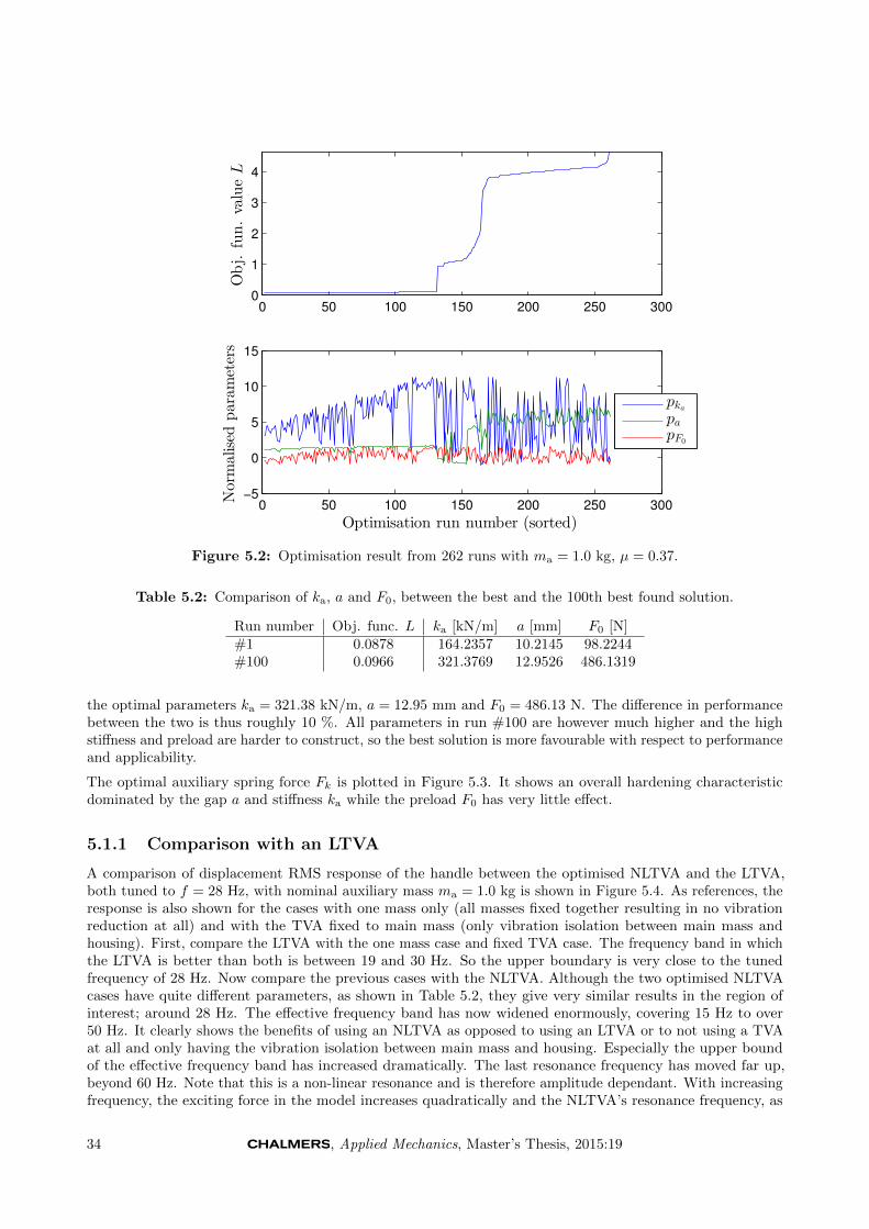
0 50 100 150 200 250 3000

1

2

3

4

Obj.

fun.valueL

0 50 100 150 200 250 300−5

0

5

10

15

Normalised

param

eters

Optimisation run number (sorted)

pkapapF0

Figure 5.2: Optimisation result from 262 runs with ma = 1.0 kg, µ = 0.37.

Table 5.2: Comparison of ka, a and F0, between the best and the 100th best found solution.

Run number Obj. func. L ka [kN/m] a [mm] F0 [N]#1 0.0878 164.2357 10.2145 98.2244#100 0.0966 321.3769 12.9526 486.1319

the optimal parameters ka = 321.38 kN/m, a = 12.95 mm and F0 = 486.13 N. The difference in performancebetween the two is thus roughly 10 %. All parameters in run #100 are however much higher and the highstiffness and preload are harder to construct, so the best solution is more favourable with respect to performanceand applicability.

The optimal auxiliary spring force Fk is plotted in Figure 5.3. It shows an overall hardening characteristicdominated by the gap a and stiffness ka while the preload F0 has very little effect.

5.1.1 Comparison with an LTVA

A comparison of displacement RMS response of the handle between the optimised NLTVA and the LTVA,both tuned to f = 28 Hz, with nominal auxiliary mass ma = 1.0 kg is shown in Figure 5.4. As references, theresponse is also shown for the cases with one mass only (all masses fixed together resulting in no vibrationreduction at all) and with the TVA fixed to main mass (only vibration isolation between main mass andhousing). First, compare the LTVA with the one mass case and fixed TVA case. The frequency band in whichthe LTVA is better than both is between 19 and 30 Hz. So the upper boundary is very close to the tunedfrequency of 28 Hz. Now compare the previous cases with the NLTVA. Although the two optimised NLTVAcases have quite different parameters, as shown in Table 5.2, they give very similar results in the region ofinterest; around 28 Hz. The effective frequency band has now widened enormously, covering 15 Hz to over50 Hz. It clearly shows the benefits of using an NLTVA as opposed to using an LTVA or to not using a TVAat all and only having the vibration isolation between main mass and housing. Especially the upper boundof the effective frequency band has increased dramatically. The last resonance frequency has moved far up,beyond 60 Hz. Note that this is a non-linear resonance and is therefore amplitude dependant. With increasingfrequency, the exciting force in the model increases quadratically and the NLTVA’s resonance frequency, as


0 2 4 6 8 10 12 14 16 18

0

200

400

600

800

1000

1200

xrel [mm]

Fk[N

]

Optimal Fk (3-par: ka, a, F0)

xrel amplitude at flb = 23.8 Hz

xrel amplitude at fub = 32.2 Hz

Figure 5.3: Auxiliary spring force Fk for optimal parameter ka, a and F0 as given in Table 5.2. The squareand triangle markers show the amplitude of the auxiliary mass relative main mass at the lower and upperexcitation frequency bounds used in the objective function.

0 10 20 30 40 50 600

0.2

0.4

0.6

0.8

1

1.2

1.4

1.6

1.8

2

Frequency [Hz]

Displacementrm

sx3[m

m]

1 massFix TVALTVANLTVA #1

NLTVA #100

Figure 5.4: Displacement RMS of the handle for five different configurations. 1 mass: the machine is modelledas one single mass of mm +ma +mh. Fix TVA: the TVA is deactivated by fixing it to the main mass, so theonly vibration reduction is from the isolation between main mass and housing. LTVA: linear system tuned to28 Hz by adjusting the auxiliary spring ka. NLTVA: non-linear system using optimised parameter set #1 and#100 from Table 5.2.


stated analytically in (2.1), is expected to increase with it. This should be the reason why the last resonanceis moved so far up. A further discussion on the assumption of quadratically increasing exciting force and itsconsequences is given in Section 5.1.3.

Plotting the phase angles, as seen in Figure 5.5, also shows the superior effect of the NLTVA. At 28 Hz theauxiliary mass is in almost perfect counterphase with the exciting force. Here the main mass (and the housing)makes a 180 phase shift in both the linear and non-linear system, however much more abrupt in the linearsystem. For the linear system, the last resonance occurs rather soon afterwards, around 34 Hz. At this point,all masses make a 180 shift and the LTVA amplifies vibration since it is no longer in counterphase with theexciting force, cf. the curves for fixed TVA and LTVA in Figure 5.4. The LTVA is thus only effective in a verynarrow band above the tuned frequency. For the non-linear system, the last resonance and phase shift comes ata very high frequency. The auxiliary mass can therefore stay close to perfect counterphase (-180) up to a muchhigher frequency than in the linear system. With the NLTVA, the lag between main and auxiliary mass around20 Hz as well as the slower shift around 28 Hz is believed to be caused mainly by the gap length a. The gapand preload are also the reason why vibration is not suppressed as much as with the LTVA exactly at the tunedfrequency 28 Hz, cf. Figure 5.4. The non-linearities basically cause a small mismatch between exciting forceand auxiliary spring force so that they cannot counteract each other perfectly. In the big picture, however, thisis unimportant since the pneumatic machine can never be assured to operate at the tuned frequency exactly.

0 10 20 30 40 50 60

−350

−300

−250

−200

−150

−100

−50

0

Frequency [Hz]

Phase

angle

[]

Main massAuxiliary massHousing

(a) System with LTVA tuned to 28 Hz.

0 10 20 30 40 50 60

−350

−300

−250

−200

−150

−100

−50

0

Frequency [Hz]

Phase

angle

[]

Main massAuxiliary massHousing

(b) System with optimised NLTVA (#1).

Figure 5.5: Phase angles of all masses taken for the excitation frequency f relative the exciting force, withauxiliary mass ma = 1.0 kg.

5.1.2 The solution’s sensitivity

The optimal parameters are delivered with very high precision from the optimisation. A precision of this kindcan of course not be used when manufacturing impact machines. To investigate how sensitive the optimalsolution is to variations in the optimal parameters a simple sensitivity analysis was performed. Each parameterwas varied from -50 % to +50 % of the optimal value and the objective function L was calculated. Theamplitude of the force Fe was also included in the sensitivity analysis because it can be influenced by operatingconditions and air pressure and between machines. The results from varying single parameters from the optimalparameters in Table 5.2, with ma = 1 kg, can be seen in Figure 5.6.

From Figure 5.6 it is clear that, for the optimal parameters used, the objective function is most sensitiveto variations in the weight of the auxiliary mass ma and the length of the gap a. The objective function issignificantly less sensitive to the amplitude of the force Fe. The preload F0 can be varied within ±50 % withoutany significant changes in the objective function. Although the sensitivity to stiffness ka is much grater than forthe preload there is a rather wide range around 0 where the changes in L are minimal. The greater sensitivityto changes in weight of the auxiliary mass ma and the gap length a should not be problematic since they arethe parameter that are easiest to control. On the other hand the sensitivity to the amplitude of the force canbe problematic, since it is hard to measure and control. The forcing amplitude should therefore be measured as


−50 0 500

50

100

150

200

250

300

350

400

450

500

Change

ofL

from

optimalvalue[%

]

Change in parameter [%]

kaaF0Fe,refma

Figure 5.6: Changes in the objective function L when a single parameter and the forcing amplitude are variedfrom the optimal values #1 from Table 5.2. The amplitude of the force is varied from it’s nominal value seen inTable 2.1 and the mass ma from its nominal value of 1 kg.

well as possible as well as investigating how it varies to be able to use a correct value and possibly include somevariation of it in the objective function for future optimisations.

5.1.3 Different exciting force assumptions

As described in Section 3.4.5, the amplitude of the exciting force is assumed to increase quadratically withexcitation frequency. To investigate how crucial this assumption is, the proposed NLTVA was also tuned forcases where the amplitude is constant, as well as with a linearly increasing amplitude. The only changes madewere that the equation for the exciting force was changed to:

|Fe(f)| = Fe,ref (5.1)

to have a constant force amplitude and

|Fe(f)| = Fe,ref · (f/fref) (5.2)

to use a linearly increasing amplitude. All other parameters and bounds used were exactly the same as inSection 5.1. The resulting parameters that gave the lowest objective function using all three equations for theamplitude of the force can be seen in Table 5.3.

Table 5.3: The parameters ka, a and F0 that gave the lowest objective function value with a constant, linearlyincreasing and quadratically increasing exciting force amplitude.

Obj. func. L ka [kN/m] a [mm] F0 [N]Constant |Fe(f)| 0.1868 256.2161 9.7451 17.3061Linear |Fe(f)| 0.1352 253.0793 10.3159 2.1978Quadratic |Fe(f)| 0.0878 164.2357 10.2145 98.2244

As can be seen in Table 5.3, the gap length a is similar in all cases. The gap length is slightly lower for a


constant force amplitude and slightly higher when a linearly increasing is used. The stiffness ka is however muchhigher for both linear and constant amplitudes than the quadratic. The preload F0 is only 2 N for the linearcase and only 17 N for the constant case. A comparison of the objective function value L for all three casesand for different system configurations can be seen in Table 5.4 and the response of the handle at frequenciesaround 28 Hz can be seen in Figure 5.7.

Table 5.4: Comparison of the lowest objective function value with a constant, linearly increasing andquadratically increasing exciting force amplitude. The difference in objective function between using theNLTVA and an LTVA is shown on the right.

Obj. func. L

Fixed TVA LTVA NLTVAReduction of L

NLTVA vs LTVA [%]Constant |Fe(f)| 1.1207 0.4880 0.1868 -61.72Linear |Fe(f)| 1.1793 0.5346 0.1352 -74.71Quadratic |Fe(f)| 1.2477 0.5913 0.0878 -85.15

15 20 25 30 35 400

0.2

0.4

0.6

0.8

1

1.2

1.4

1.6

1.8

2

Frequncy f [Hz]

Displacementx3rm

s[m

m]

Fix. TVALTVANLTVA

(a) Constant force amplitude |Fe(f)|, according to (5.1).

15 20 25 30 35 400

0.2

0.4

0.6

0.8

1

1.2

1.4

1.6

1.8

2

Frequncy f [Hz]

Displacementx3rm

s[m

m]

Fix. TVALTVANLTVA

(b) Linearly increasing force amplitude |Fe(f)|, accordingto (5.2).

15 20 25 30 35 400

0.2

0.4

0.6

0.8

1

1.2

1.4

1.6

1.8

2

Frequncy f [Hz]

Displacementx3rm

s[m

m]

Fix. TVALTVANLTVA

(c) Quadratically increasing force amplitude |Fe(f)|, ac-cording to (3.18).

Figure 5.7: Response of the housing for different formulations of exciting force amplitude |Fe(f)|. Comparisonbetween having the TVA fixed to main mass, LTVA and NLTVA.


Figure 5.7 shows that the NLTVA gives a much wider suppression band than an LTVA for all cases. Table 5.4shows that the reduction in the objective function is over 60 % for all cases. An interesting finding is that thereduction is lowest for the constant amplitude, a bit greater for the linearly increasing amplitude and greatestfor the quadratically increasing amplitude.

Resonance frequency for different exciting force amplitudes

Equation (2.1) shows that the resonance frequency fres of the NLTVA depends on the spring compression b. Toinvestigate where the NLTVA is operating with regards to the resonance frequency, the analytical resonancefrequency was calculated. The spring compression b was taken from the simulation and the resonance frequencywas calculated using (2.1) for the different force amplitudes |Fe(f)|. Comparison between the working frequencyand the operating frequency, for all cases using the optimal parameters in Table 5.3, can be seen in Figure 5.8.

20 25 30 35 40 4520

25

30

35

40

45

Analytical

resonan

cefrequen

cyfres[H

z]

20 25 30 35 40 452

6

10

14

18

22

Com

pressionof

theNLTVA

springb[m

m]

Operating frequency f [Hz]

f

fres

b

(a) Constant force, according to (5.1).

20 25 30 35 40 4520

25

30

35

40

45

Analytical

resonan

cefrequen

cyfres[H

z]

20 25 30 35 40 452

6

10

14

18

22

Com

pressionof

theNLTVA

springb[m

m]


f

fres

b

(b) Linearly increasing force, according to (5.2).

20 25 30 35 40 4520

25

30

35

40

45

Analytical

resonan

cefrequen

cyfres[H

z]

20 25 30 35 40 452

6

10

14

18

22

Com

pressionof

theNLTVA

springb[m

m]


f

fres

b

(c) Quadratically increasing force, according to (3.18).

Figure 5.8: Analytical resonance frequency fres versus the operating frequency f , for different formulations ofthe exciting force amplitude |Fe(f)|. The operating frequency is plotted against itself, with a dashed line, asan ideal reference case. The compression of the NLTVA’s spring b, which is used to calculate the resonancefrequency, is plotted with a dash-dot line. The scale on the right y-axis belongs to b.

The operating frequency is plotted against itself as a reference. This straight line is used as a reference becausewhen the resonance frequency fres is the same as the operating frequency f , the NLTVA gives (theoretically)maximum suppression. The compression b is also plotted with a secondary y-axis on the right.

As can be seen in Figure 5.8c the operating frequency f is very close to the resonance frequency over a widefrequency range when a quadratically increasing exciting force amplitude is used. It is slightly below the


resonance frequency fres when the machine is operated below 33 Hz and when the operating frequency f movespast 33 Hz it overtakes the resonance frequency. When the forcing amplitude grows linearly, cf. Figure 5.8b,the difference between the operating frequency f and the resonance frequency fres is larger for both the lowerand higher frequencies and when a constant force amplitude is used, cf. Figure 5.8a, the difference is evengreater. This difference between the three cases is most likely the reason for the larger difference betweenthe performance of an NLTVA vs. an LTVA seen in Table 5.4 when a quadratically increasing exciting forceamplitude |Fe(f)| is used.

5.2 Sensitivity to mass ratio

To investigate how the weight of the auxiliary mass affects the performance of the NLTVA, the model wasoptimised multiple times with 9 different values of ma. Lighter masses were chosen because HHIMs in generalare desired to be as light as possible for easier handling and better ergonomics. As conventionally done inliterature, the weight of the auxiliary mass is expressed relative the main mass as the mass ratio µ defined as:

µ =ma

mm(5.3)

The optimised parameters, ka, a and F0, that gave the lowest value of the objective function L for all 9mass ratios can be seen in Table 5.5 and the value of the objective function versus mass ratio can be seen inFigure 5.9.

Table 5.5: Optimised parameter changes and the corresponding objective function values L for different massratios µ. The reference value Lref = 1.248 is the value of the objective function with vibration isolation and afixed TVA.

ma [kg] µ ka,opt [kN/m] aopt [mm] F0,opt [N] L ∆L/Lref [%]1.0 0.3704 164.2357 10.2145 98.2244 0.0878 -92.96590.9 0.3333 157.3752 11.3816 76.7169 0.0917 -92.65120.8 0.2963 140.5606 12.7339 70.5280 0.0975 -92.18760.7 0.2593 105.5335 14.3572 128.8133 0.1072 -91.40870.6 0.2222 95.4965 16.3216 74.2882 0.1201 -90.37340.5 0.1852 75.4409 18.1274 4.5437 0.1436 -88.49340.4 0.1481 49.5826 21.9811 75.6339 0.1893 -84.82470.3 0.1111 38.5226 27.3383 28.8508 0.2833 -77.29490.2 0.0741 13.1234 27.8495 80.0670 0.5362 -57.0270

When looking at the best parameters for different mass ratios, cf. Table 5.5, two trends can be seen. First theexpected reduction in stiffness ka when the mass ratio is decreased and secondly that the gap gets larger whenthe mass ratio is decreased. No clear trend can be seen for the value of the preload, except that it is alwayslower than the nominal value of 190 N. The lack of a trend correlates well with the low sensitivity to preload inthe case of 1 kg auxiliary mass, as previously seen in Figure 5.6.

Figure 5.9 clearly shows the benefit of having a higher mass ratio. A more surprising finding is however thatthe growth of L, with decreased mass ratio µ is very gradual down to µ = 0.2222, but when the mass ratio isdecreased further the growth becomes much more rapid. To investigate this further, it was necessary to lookat the response of the housing, that is used to calculate the objective function, as well as the velocity anddisplacement of the auxiliary mass. The response, as calculated in the objective function during optimisation,can be seen in Figure 5.10 and the displacement and velocity amplitudes of the auxiliary mass relative to themain mass in Figure 5.11.

Inspection of the response of the housing, for the frequencies used during the optimisation, seen in Figure 5.10,shows that the response is as expected for the higher mass ratios but for the lower mass ratios the NLTVAseems to be out of tune, i.e. the response does not have a minimum at 28 Hz.

Figure 5.11 shows that the amplitudes of both the displacement and velocity of the auxiliary mass relative tothe main mass grow with frequency. The displacement and velocity are also higher for lower mass ratio whichis expected since a lighter auxiliary mass needs a higher velocity to create the same counter force on the main


0.05 0.1 0.15 0.2 0.25 0.3 0.35 0.4−95

−90

−85

−80

−75

−70

−65

−60

−55

Mass ratio µ

Red

uctionof

theob

jectivefunctionL

[%]

Figure 5.9: Minimised objective function L for different mass ratios µ. Reduction in L is given relative thereference value Lref = 1.248 which is pertinent to a system with vibration isolation and a fixed TVA. Theresults are obtained from over 250 optimisation starts for each mass ratio.

24 25 26 27 28 29 30 31 320

0.01

0.02

0.03

0.04

0.05

0.06

0.07

Frequency [Hz]

Velocity

x3rm

s[m

/s]

µ = 0.074µ = 0.111µ = 0.148µ = 0.185µ = 0.222µ = 0.259µ = 0.296µ = 0.333µ = 0.370

Figure 5.10: Velocity RMS response of the housing in the frequency range of interest for different mass ratiosµ. For each mass ratio, the optimal parameters from Table 5.5 are used.

23 24 25 26 27 28 29 30 31 32 3310

20

30

40

50

60

70

80

Frequency [Hz]

Relativedisplacementam

plitudexrel[m

m]

µ = 0.074µ = 0.111µ = 0.148µ = 0.185µ = 0.222µ = 0.259µ = 0.296µ = 0.333µ = 0.370

(a) Displacement amplitude.

23 24 25 26 27 28 29 30 31 32 330

2

4

6

8

10

12

14

Frequency [Hz]

Relative

velocity

amplitudexrel[m

/s]

µ = 0.074µ = 0.111µ = 0.148µ = 0.185µ = 0.222µ = 0.259µ = 0.296µ = 0.333µ = 0.370

(b) Velocity amplitude.

Figure 5.11: Amplitudes of the auxiliary mass relative the main mass in the frequency range of interest fordifferent mass ratios µ. For each mass ratio, the optimal parameters from Table 5.5 are used.


mass. Having a higher velocity does however increase the dissipation through viscous damping resulting in lessvibration suppression when the mass ratio is lowered. Another interesting thing worth mentioning is that thegrowth of the auxiliary mass amplitude with frequency is much steeper for lower mass ratio. That depends onthe lower optimal stiffnesses ka,opt obtained for the lower mass ratios as seen in Table 5.5.

5.2.1 Chaotic behaviour with low mass ratios

As described in Section 3.3.2, the response in the computational model is calculated for the first frequencyusing a defined initial state z0. When the motion stabilises, the last state at that frequency is used as theinitial state at the next frequency to reduce the time needed to stabilise into a limit cycle at each frequency.The stable motion of a non-linear system can however depend heavily on the initial state, i.e. there can existseveral limit cycles, and in certain cases the motion will not stabilise at all and instead be chaotic.

To investigate how changes in the initial state affect the solution, two tests were performed. The first approachwas to evaluate the response backwards, i.e. starting at the highest frequency of interest (32.2 Hz), with theinitial state z0, and continue to use the final state at that frequency as the initial state at the frequency below.This analysis showed that the response is identical for mass ratios µ ≥ 0.158 but for the three lowest massratios the response is different. Comparison between beginning at the highest and lowest frequency can be seenin Figure 5.12 for µ = 0.074, 0.111 and 0.148.

22 24 26 28 30 32 340.02

0.04

0.06

0.08

0.1

0.12

0.14

0.16

0.18

Frequency [Hz]

Velocity

x3rm

s[m

/s]

Fixed auxiliary mass

NLTVA, f →

NLTVA, f ←

(a) µ = 0.074.

22 24 26 28 30 32 340

0.02

0.04

0.06

0.08

0.1

0.12

0.14

0.16

0.18

0.2

Frequency [Hz]

Velocity

x3rm

s[m

/s]


NLTVA, f →

NLTVA, f ←

(b) µ = 0.111.

22 24 26 28 30 32 340

0.02

0.04

0.06

0.08

0.1

0.12

0.14

0.16

0.18

Frequency [Hz]

Velocity

x3rm

s[m

/s]


NLTVA, f →

NLTVA, f ←

(c) µ = 0.148.

Figure 5.12: Response of the housing within the frequency range of interest by the optimisation for differentmass ratios µ. Comparison between starting at the highest frequency vs the lowest.


Figure 5.12 shows that when the simulation goes down the frequency range, different response curves areobtained. When the response, beginning at the highest frequency is compared with the response of the systemwith fixed auxiliary mass we see that the vibrations are greater, i.e. the TVA has switched from reducingthe vibration of the handle to increasing vibration. This unwanted behaviour continues to the second lowestfrequency when µ = 0.074, seen in Figure 5.12a. At the lowest frequency, the response drops down to thesame value as when the response is calculated from the lowest frequency. Therefore the stability of thevibrations seems to be independent of the initial state for the lowest frequency. This stabilisation similarlyhappens between 24.9 and 25.7 Hz when µ = 0.111. When µ = 0.148, the chaotic motion only occurs for thehighest frequency. Comparison between the highest and second highest frequency, with µ = 0.148 and optimalparameters, can be seen in Figure 5.13. The time history is displayed in Figure 5.13a and 5.13b for 31.11 Hzand 32.2 Hz respectively. Note that the chaotic response at 32.2 Hz is only displayed between 6 and 7.5 s toshow the typical chaotic response. Phase space plots from the same data are shown in Figure 5.13c and 5.13dfor 31.11 and 32.2 Hz respectively. Note that the phase space plots only include the very last part of the timehistory that is used to evaluate the RMS during the computation.

0 0.5 1 1.5 2 2.5 3 3.5 4−0.09

−0.08

−0.07

−0.06

−0.05

−0.04

−0.03

−0.02

−0.01

0

0.01

t [s]

Displacement[m

]

31.11 Hz, 59449 time steps

Main massAux. massHousing

(a) Response of the system at f = 31.11 Hz until thevibrations become stable with optimal parameters, µ =0.148.

6 6.5 7 7.5−0.08

−0.07

−0.06

−0.05

−0.04

−0.03

−0.02

−0.01

t [s]

Displacement[m

]

32.20 Hz, 112289 time steps


(b) Typical chaotic response of the system at f =32.20 Hz with optimal parameters, µ = 0.148.

−0.08 −0.07 −0.06 −0.05 −0.04 −0.03 −0.02 −0.01 0−6

−4

−2

0

2

4

6 Phase space

x [m]

v[m

/s]

Main mass

Aux. mass

Housing

(c) Phase space plot of the vibrations seen in 5.13a.

−0.07 −0.06 −0.05 −0.04 −0.03 −0.02 −0.01−3

−2

−1

0

1

2

3

4 Phase space

x [m]

v[m

/s]


(d) Phase space plot of the vibration seen in 5.13b.

Figure 5.13: Comparison between stable and chaotic vibrations for µ = 0.148. When the system is simulatedfrom the lowest frequency to the highest.

The second test was to calculate the response individually for each frequency always with the initial state z0.This gave chaotic behaviour at the same frequencies as in the first test for all mass ratios.

Some efforts were made, for the lower mass ratios, to move the minimum of the response lower in frequency,i.e. tuning it to 28 Hz, by increasing the gap and lowering the stiffness manually. These efforts all resultedin a chaotic response within the frequency range of interest, even when starting at the lowest frequency andstepping upwards as usual. This suggests that the optimisation finds the parameters that give the lowest


eigenfrequency, without introducing chaotic response within the frequency range of interest. With the lowestmass ratios though, the system seem to be very sensitive to initial condition and will probably be infeasible inreality.

The results show that the proposed NLTVA can work well for lower mass ratios. Lowering the mass ratio doeshowever reduce the vibration suppression. For very low mass ratios, chaotic response can be an issue and mighteven cause increased vibration, at least for the large exciting force that is used in this thesis.

5.3 Free damping

The results in the previous section showed that chaotic behaviour can occur when the mass ratio is lowered. Asshown in Figure 5.11b, a light auxiliary mass needs to move at a higher velocity and is therefore more affectedby the damping. To investigate what would be the optimal damping for the lightest auxiliary mass ma = 0.2 kgand to see if the chaotic behaviour could be avoided if the damping was lowered further, an optimisation wasperformed with the damping ca as a fourth free parameter. The parameter bounds that were used duringoptimisation can be seen in Table 5.6.

Table 5.6: Physical values of the free parameters in optimisation with free damping ca.

Parameter Nominal value Lower bound Upper boundka [kN/m] 40 0 500a [mm] 5 0 40F0 [N] 190 0 700

ca [N s/m] 1 -30 30

Negative damping was allowed due to interest from the supervisor to see if it could improve the performance.The equivalence of negative damping could be achieved by using the outlet air from the impact mechanism togive the auxiliary mass a boost.

The parameter values that minimised the objective function can be seen in Table 5.7 and a comparison betweenthe optimised NLTVA with free damping, nominal damping, LTVA and fixed TVA can be seen in Figure 5.14.

Table 5.7: The parameters that gave the lowest value of the objective function L when the damping ca wasfree and the auxiliary mass ma = 0.2 kg.

ka,opt [kN/m] aopt [mm] F0,opt [N] ca,opt [N s/m]11.351 36.7 188 0.0857

As can be seen in Table 5.7, the damping becomes negligibly low but not negative. Very low damping wasexpected since the performance of TVAs is generally better when there is no damping present. Compared tothe previous case where the damping is fixed to its nominal value ca = 1 N s/m, cf. Table 5.5, the stiffnesska is slightly lower but approximately the same. The gap length a and preload F0 are however significantlylarger. The increase in the gap length is expected since the auxiliary damping here is close to zero and thereforethe NLTVA’s dissipation of vibration energy is very low. Figure 5.14 shows that the NLTVA with optimiseddamping is better tuned to the target frequency, i.e. the minimum lies closer to 28 Hz. The vibration is alsosignificantly lower when the damping is smaller.

Chaotic vibrations appeared at the same frequencies as in Section 5.2.1 if the response was calculated from thehighest frequency to the lowest and if single frequencies where calculated, which suggests that lowering thedamping ca does not reduce the risk of chaotic motion.


23 24 25 26 27 28 29 30 31 32 330

0.05

0.1

0.15

0.2

0.25

Frequency [Hz]

Velocity

x3rm

s[m

/s]

Housing, NLTVA with ca,opt

Housing, NLTVA, ca = 1 [Ns/m]

Housing, LTVA, ca = 1 [Ns/m]

Housing, fix TVA

Figure 5.14: Response of the housing within the frequency range of interest. Comparison between optimisationresult for the NLTVA with free ca and the nominal value as well an LTVA and fixed auxiliary mass.

5.4 Free auxiliary mass

In another batch of optimisation runs, the auxiliary mass was allowed free. That is the four parameters ka,a, F0 and ma were allowed to be varied for optimisation. The bound values set in the optimisation for thesefree parameters are shown in Table 5.8. The resulting sorted objective function values and correspondingparameters are shown in Figure 5.15 and the parameters that minimised the objective function can be seen inTable 5.9.

Table 5.8: Physical values of the free parameters in optimisation.

Parameter Nominal value Lower bound Upper boundka [kN/m] 40 0 500a [mm] 5 0 40F0 [N] 190 0 500ma [kg] 1 0.1 3

Table 5.9: The parameters that gave the lowest value of the objective function L when the the auxiliary massma was free.

Obj. func. L ka,opt [kN/m] aopt [mm] F0,opt [N] ma,opt [kg]0.0748 273.464 4.5 52 2.0878

The optimisation results seen in Figure 5.15 are similar to the results when ma was fixed, i.e. a large proportionof the runs resulted in a very low objective function, and the stiffness ka, and preload F0 vary significantlyamong the good results. Another interesting thing is that none of the results with a very low objective functionlie on the upper bound of 3 kg for ma. Most of them do however lie close to a normalised value of pma

= 1giving an auxiliary mass ma around 2 kg. As seen in Table 5.9 the best parameter set has ma = 2.0878 kgand gives an objective function value of L = 0.0748. This low objective function value fits the trend seen inSection 5.2, i.e. heavier auxiliary mass gives more suppression. The interesting fact is however that the upperbound on the auxiliary mass ma was set to 3 kg. This suggests that there is a limit to the improvement possible


0 200 400 600 800 1000 12000

2

4

6

8

Obj.

fun.valueL

0 200 400 600 800 1000 1200−5

0

5

10

15

Normalised

param

eters

Optimisation run number (sorted)

pkapapF0

pma

Figure 5.15: Optimisation result from 1038 runs with the weight of the auxiliary mass ma as a free parameter.

by increasing the auxiliary mass. When put in perspective with the weight of the main mass, the optimal massratio is:

µ =2.0878 kg

2.7 kg= 0.773

So the auxiliary mass can hardly be considered an auxiliary mass since its weight is such a large proportion ofthe total mass of the system.

5.5 Removing a resonance with the proposed NLTVA

Traditionally, the common use of TVAs is to remove or minimise the response at an unwanted resonance. Thisis desirable when a system is excited at its resonance frequency, as opposed to the studied prototype machinein which the operating frequency is well above all of the primary system’s resonances. To investigate theproposed NLTVA’s ability to be used in this sense, a case study was performed. All model parameters exceptthe main stiffness km were kept the same as in other parts of the project. The housing was however removedfrom the model to make the study more general. There was thus only two masses in the model as illustrated inFigure 5.16.

The stiffness km between the ground and the main mass was set to

km = (2π · 28)2 ·mm (5.4)

in order for the eigenfrequency of the primary system to be 28 Hz. The stiffness ka, gap length a and preloadF0 were then optimised using the same objective function as earlier, for ma = 1.0, 0.7 and 0.3 kg.

A comparison of the response of the main mass between 1 and 60 Hz with an NLTVA, LTVA and without TVAcan be seen in Figures 5.17, 5.18 and 5.19 for ma = 1.0, 0.7 and 0.3 kg respectively. The wider suppressionband of the NLTVA can be seen clearly in these figures. For the lighter mass, a strange peak is shown around35 Hz. To find the reason for this small peak, the time history was studied at these frequencies. A typicalexample of the motion can be seen in Figure 5.20. Looking at the time history in Figure 5.20, one sees how theamplitude of the displacement of the main mass varies periodically with a frequency that is one fifth of the


mm

ma

x2(t)

x1(t)Fe(t)

cm

ka, a, F0ca

kmx

Figure 5.16: 2-DOF model with only main mass and auxiliary mass.

main frequency or 6.5 Hz. Therefore the amplitude of the displacement of main mass varies with the samefrequency giving a higher RMS value than at frequencies where the amplitude is constantly low. Although thisslight beat is present, the vibration is still much lower than when the LTVA is used up to 50 Hz for both the0.7 and 0.3 kg auxiliary mass. After the resonance around 55 Hz, the motion becomes chaotic and the level ofvibration is slightly higher than when an LTVA or no TVA is used. This shows that the non-linearities presentcan be beneficial to reduce a resonance, if the system has quadratically increasing excitation as used here andthe excitation frequency does not go too high above the resonance frequency. In this case, excitations above40 Hz give increased vibration compared to the system without the NLTVA.

For more general results and conclusions, this study should be continued by investigating different damping andexciting force scenarios. For example, optimisation should be performed with several different values of maindamping cm and auxiliary damping ca. It should also include different exciting force assumptions; constant,linearly increasing and quadratically increasing exciting force amplitude.

0 10 20 30 40 50 600

2

4

6

8

10

12

14

16

18

Frequency [Hz]

Displacementx1rm

s[m

m]

NLTVALTVANo TVA

Figure 5.17: Response of the main mass when the resonance between the ground and the main mass hasbeen set to 28 Hz. The response is shown without a TVA, with an optimised NLTVA and an LTVA. ma = 1 kg.Note that the amplitude of the force grows quadratically.


0 10 20 30 40 50 600

2

4

6

8

10

12

14

16

18

Frequency [Hz]

Displacementx1rm

s[m

m]

NLTVALTVANo TVA

Figure 5.18: Response of the main mass when the resonance between the ground and the main mass hasbeen set to 28 Hz. The response is shown without a TVA, with an optimised NLTVA and LTVA. ma = 0.7 kg.Note that the amplitude of the force grows quadratically.

0 10 20 30 40 50 600

2

4

6

8

10

12

14

Frequency [Hz]

Displacementx1rm

s[m

m]

NLTVALTVANo TVA

Figure 5.19: Response of the main mass when the resonance between the ground and the main mass hasbeen set to 28 Hz. The response is shown without a TVA, with an optimised NLTVA and LTVA. ma = 0.3 kg.Note that the amplitude of the force grows quadratically.


8 8.1 8.2 8.3 8.4 8.5 8.6−0.06

−0.04

−0.02

0

0.02

0.04

0.06

t [s]

Displacement[m

]

32.50 Hz

Main massAux. mass

Figure 5.20: Example of time history of the motion at the small peak for ma = 0.3 kg. The amplitude of thedisplacement of the auxiliary mass varies sinusoidally with a frequency one fifth of the operating frequency.

6 Conclusions

The main goal of the project was to optimise the performance of the NLTVA currently in use in the prototypeP3B. A numerical Matlab model has been built that predicts the vibration of the machine by solving thenon-linear 3-DOF equation of motion using a built-in ODE solver. Investigation of the model showed thatthe error tolerances on the numerical solution had to be tighter than the default ones in Matlab to givetrustworthy results. The model was verified against analytical results and validated against experimental datafrom the prototype. Comparison of different ODE solvers showed that ode45 with tightened error tolerancesperformed best, i.e. it solved the ODE fastest with high accuracy. The calculation time was reduced further bymaking the auxiliary spring force acting between the auxiliary mass and the main mass continuous and smoothat all points. This was achieved using a third order polynomial in the areas of non-smoothness. The excitingforce was measured experimentally to give a realistic input in the model. It was approximated as a sinusoidalforce and assumed to increase quadratically in amplitude with excitation frequency.

An objective function was defined in such way that it sums up the level of vibration around the nominaloperating frequency, thus taking into account the possible variations in the operating frequency. The frequencypoints used are distributed around the nominal frequency using a normal distribution, thereby putting moreemphasis on minimising the response in the region closest to the nominal operating frequency. The minimisationfunction lsqnonlin was used to minimise the vibration of the handle at the frequencies defined in the objectivefunction. The three parameters subject to optimisation were spring stiffness ka, gap length a and spring preloadF0. The optimisation results for the current prototype suggests that the level of suppression and the width ofthe suppression band can be increased significantly. The optimal solutions were highly non-linear and includeda significant increase in the gap length a and the spring stiffness ka which suggests that the best performanceis achieved when the auxiliary mass barely compresses the springs to create a counterforce. That means thatthe auxiliary mass is bouncing against the main mass in an impact-like manner.

A comparison has been made between different ways of varying the amplitude of the exciting force withoperating frequency. The formulations used were; quadratically increasing, linearly increasing and a constantamplitude. The results show that the NLTVA gives a much wider suppression band than an LTVA for allthe amplitude formulations tested. The superiority of the NLTVA is greatest when a quadratically increasingamplitude is used, slightly less for a linearly increasing amplitude and yet a bit smaller for a constant amplitude.


A likely reason for this superiority of the NLTVA is that its resonance frequency moves up with the operatingfrequency as it increases. The operating frequency and the resonance frequency stay closest together when theamplitude increases quadratically.

Optimisations with lower mass ratios showed that the vibration suppression decreases with a lighter auxiliarymass. That relation was as expected but the more surprising finding was that the decrease in suppression is verygradual down to ma = 0.6 kg, but below that the performance decreases much more rapidly. For auxiliary massweights below 0.5 kg the initial state was critical, i.e. the response became chaotic in certain cases. Anotherinteresting finding regarding the weight of the auxiliary mass was that, when the optimisation was performedwith the weight of the auxiliary mass as a free parameter with an upper bound at 3 kg, the lowest values of theobjective function were obtained when ma was around 2 kg. This suggests that there is a limit on how muchthe performance of the NLTVA can be improved by increasing the weight of the auxiliary mass.

A study was performed to investigate the proposed NLTVA’s performance when it comes to the traditionaltask, to suppress a resonance in a system. The study showed that, for the exciting force used, the suppressionat the target frequency was almost as good as when an LTVA is used but the suppression band is much wider.For lighter auxiliary masses, slight beats were observed above the target frequency but although those beatsgave a reduction in vibration suppression, the suppression at these frequencies was still much better than ifan LTVA was used. An interesting further investigation would be to consider resonance removal for differentexcitation forces numerically and validate the results experimentally if they suggest that the NLTVA is superiorto the LTVA.

Unfortunately, none of the results from the optimisations have been validated against test data from theprototype. That is a matter for future work. Therefore the question whether the already low vibration ofthe prototype will decrease significantly in reality if the parameters from the optimisation are used remainsunanswered. The results do however strongly suggest that it will. Validation should be done by tuningthe available prototype using the optimised parameters and measure if the level of vibration becomes lowerthan it already is. If these experiments agree with the optimisation results presented, the NLTVA can beoptimised and implemented on reciprocating machines of other dimensions and characteristics rather easilywith the help of the developed Matlab code. Since the sensitivity analysis showed that the tuned frequencyis sensitive to the amplitude of the exciting force, variations of it should be accounted for in the objective function.

7 Recommendations

The optimisations showed that a very low objective function can be achieved using a variety of parameter sets.The parameter sets are however delivered with such high precision that manufacturing the NLTVA could beproblematic. One obvious problem is that manufacturing a spring that has a stiffness over 250 kN/m with aprecision of less than 1 kN/m would be very expensive and complex, if possible at all. An approach to solvethis problem would be to decide the combination of parameters in three steps:

1. Run an optimisation where all three parameters are free and sufficiently broad bounds.

2. Inspect the parameter sets that give a low objective function value L and pick out a value of ka. Thevalue would then be compared to available springs. Choose the spring with a stiffness closest to thechosen ka.

3. Run another optimisation using the stiffness of the chosen spring as a fixed parameter and the preload F0

and gap length a as free parameters with rather tight bounds around the values obtained in step 1. Thiswill give more correct values for these parameters to use with the chosen spring.

This method should give good results since the preload F0 and gap length a are much more controllable thanthe stiffness ka. Using this method should therefore minimise the loss of vibration suppression due to using aspring that is not exactly as stiff as the solution recommends.


References

[1] T. Nilsson. “Arbete med handhallna vibrerande maskiner och skadlig exponering”. Arbetssjukdom -skadlig inverkan - samband med arbete. Ett vetenskapligt underlag for forsakringsmedicinska bedomningar(sju skadeomraden). Arbete och Halsa. Ed. by P. Westerholm. 15. Stockholm: Arbetslivsinstitutet, 2002,pp. 245–271.

[2] P. Rehfisch and R. Walinder. ABC om vibrationsskador. Lakartidningen 106.7 (2009), 439–442.[3] R. E. Roberson. Synthesis of a nonlinear dynamic vibration absorber. Journal of the Franklin Institute

254.3 (1952), 205–220.[4] H. Lindell. “Impact machine”. WO2014095936A1. 2014.[5] H. Lindell. Redesign of hand-held impact machines to reduce hand-arm vibration. Canadian Acoustics

39.2 (2011), 80–81.[6] H. Lindell. Vibrationer i stenindustrin. Slutrapport. Swerea IVF, 2012.[7] H. Frahm. “Device for damping vibrations of bodies”. US989958. 1911.[8] J. Ormondroyd and J. P. Den Hartog. Theory of the dynamic vibration absorber. Transactions of the

American Society of Mechanical Engineers 50.7 (1928), 11–22.[9] J. P. Den Hartog. Mechanical vibrations. 4th ed. 1956.

[10] K. Y. Hao, L. X. Mei, and Z. M. Ripin. Tuned vibration absorber for suppression of hand-arm vibrationin electric grass trimmer. International Journal of Industrial Ergonomics 41.5 (2011), 494–508.

[11] K. Y. Hao and Z. M. Ripin. Nodal control of grass trimmer handle vibration. International Journal ofIndustrial Ergonomics 43.1 (2013), 18–30.

[12] L. A. Pipes. Analysis of a nonlinear dynamic vibration absorber. Journal of Applied Mechanics 20 (1953),515–518.

[13] F. R. Arnold. Steady-state behavior of systems provided with nonlinear dynamic vibration absorbers.Journal of Applied Mechanics 22.4 (1955), 487–492.

[14] J. Hunt and J.-C. Nissen. The broadband dynamic vibration absorber. Journal of Sound and Vibration83.4 (1982), 573–578.

[15] M. Wang. Feasibility study of nonlinear tuned mass damper for machining chatter suppression. Journalof Sound and Vibration 330.9 (2011), 1917–1930.

[16] G. Schlesak et al. “Variation of the natural frequency of vibratory means in electric tools”. US20120279741.2012.

[17] J. Hecht et al. “Hand-held power tool”. US8434565. 2013.[18] F. Moessnang. “Oscillation damper for hand-held power tool”. US8066106. 2011.[19] F. Moessnang. “Hand-held power tool with an oscillation damper”. US7712548. 2010.[20] The Nonlinear Tuned Vibration Absorber, The European Research Council (ERC). url: http://erc.

europa.eu/nonlinear-tuned-vibration-absorber (visited on 2015-04-13).[21] T. Detroux et al. Performance, robustness and sensitivity analysis of the nonlinear tuned vibration

absorber. Mechanical Systems and Signal Processing 60–61 (2015), 799–809.[22] G. Habib et al. Nonlinear generalization of Den Hartog’s equal-peak method. Mechanical Systems and

Signal Processing 52–53 (2015), 17–28.[23] L. Burstrom, R. Lundstrom, and A. Sorensson. “Kunskapsunderlag for atgarder mot skador och besvar

i arbete med handhallna vibrerande maskiner. Tekniska Aspekter.” Arbete och Halsa. 17. Stockholm:Arbetslivsinstitutet, 2000.

[24] Arbetsmiljoverkets forfattningssamling. AFS 2005:15 - Vibrationer. 2005.[25] European Parliament, Council of the European Union. Directive 2002/44/EC - vibration. 2002. url:

https://osha.europa.eu/en/legislation/directives/exposure-to-physical-hazards/osh-

directives/19 (visited on 2015-01-20).[26] ISO 5349-1, 2001. Mechanical vibration – Measurement and evaluation of human exposure to hand-

transmitted vibration – Part 1: General Requirements.[27] E. Golysheva, V. Babitsky, and A. Veprik. Vibration protection for an operator of a hand-held percussion

machine. Journal of Sound and Vibration 274.1–2 (2004), 351–367.[28] A. Fischer, R. Meuer, and M. Weber. “Hand-held power tool”. US8443912. 2013.[29] S. R. Henriksson and O. B. S. Ostenssn. “Impact tool with a movably supported impact mechanism”.

US7614460. 2009.[30] N. Hahn. “Vibration dampening mechanism”. US7451833. 2008.


http://erc.europa.eu/nonlinear-tuned-vibration-absorber

http://erc.europa.eu/nonlinear-tuned-vibration-absorber

https://osha.europa.eu/en/legislation/directives/exposure-to-physical-hazards/osh-directives/19

https://osha.europa.eu/en/legislation/directives/exposure-to-physical-hazards/osh-directives/19

[31] V. Babitsky. Hand-held percussion machine as discrete non-linear converter. Journal of Sound andVibration 214.1 (1998), 165–182.

[32] E. Golycheva, V. Babitsky, and A. Veprik. Dynamic correction of excitation in hand-held electro-pneumaticpercussion machines. Journal of Sound and Vibration 259.4 (2003), 829–843.

[33] I. Sokolov, V. Babitsky, and N. Halliwell. Hand-held percussion machines with low emission of hazardousvibration. Journal of Sound and Vibration 306.1–2 (2007), 59–73.

[34] ISO 28927-10, 2009. Hand-held portable power tools – Test methods for evaluation of vibration emission –Part 10: Percussive drills, hammers and breakers.

[35] MATLAB Documentation. ode45. Version R2015a. Mathworks, 2015. url: http://se.mathworks.com/help/matlab/ref/ode45.html (visited on 2015-02-02).

[36] MATLAB Documentation. Least-Squares (Model Fitting) Algorithms. Trust-Region-Reflective LeastSquares. Version R2015a. Mathworks, 2015. url: http://se.mathworks.com/help/optim/ug/least-squares-model-fitting-algorithms.html#broz0i4 (visited on 2015-04-07).

[37] A. Nilsson and T. Ostgardh. “Verifiering av matematisk modell for vibrationsdampare”. Bachelor’s thesis.Chalmers University of Technology, 2014.

[38] F. A. Mussa-Ivaldi, N. Hogan, and E. Bizzi. Neural, mechanical, and geometric factors subserving armposture in humans. The Journal of Neuroscience 5.10 (1985), 2732–2743.

[39] T. Tsuji et al. Human hand impedance characteristics during maintained posture. Biological Cybernetics72.6 (1995), 475–485.

[40] MATLAB Documentation. When the Solver Fails. Version R2015a. Mathworks, 2015. url: http://se.mathworks.com/help/optim/ug/when-the-solver-fails.html (visited on 2015-04-07).

[41] MATLAB Documentation. Improving Performance with Parallel Computing. Version R2015a. Mathworks,2015. url: http://se.mathworks.com/help/optim/ug/improving-performance-with-parallel-computing.html (visited on 2015-02-02).


http://se.mathworks.com/help/matlab/ref/ode45.html

http://se.mathworks.com/help/matlab/ref/ode45.html

http://se.mathworks.com/help/optim/ug/least-squares-model-fitting-algorithms.html#broz0i4

http://se.mathworks.com/help/optim/ug/least-squares-model-fitting-algorithms.html#broz0i4

http://se.mathworks.com/help/optim/ug/when-the-solver-fails.html

http://se.mathworks.com/help/optim/ug/when-the-solver-fails.html

http://se.mathworks.com/help/optim/ug/improving-performance-with-parallel-computing.html

http://se.mathworks.com/help/optim/ug/improving-performance-with-parallel-computing.html

A Derivation of analytical formulas for the non-linear

auxiliary system

In this chapter, an exact analytical formula for the resonance frequency of the non-linear auxiliary systemwith spring stiffness ka, gap a and preload F0 is derived for the case of no damping or gravity. Due to thenon-linearity, the resonance frequency depends on the vibration amplitude. Assuming that the main mass iscompletely still when considering the 2-DOF case (both main mass and auxiliary mass) leads to a formula forthe vibration amplitude of the auxiliary mass as a function of exciting force amplitude. These results can beused to tune a non-linear TVA to a certain frequency at a certain exciting force amplitude.

Consider free vibration of the auxiliary system in Figure A.1, i.e. without damping and exciting force. Alsoneglect gravity force. One vibration period time T can be divided into two distinct parts: when the auxiliarymass is not in contact with the main mass and when the auxiliary spring is compressing. Denote the timebetween positions I and II in Figure A.1 as ta. Denote the time from position II to position III and back as tb,cf. Figure A.2. A complete period is then given by

T = 2ta + 2tb (A.1)

2a

ka, F0ma

(a) Position I.

2a

x

(b) Position II, x = 0.

2a+ b

(c) Position III, x = b, x = 0.

Figure A.1: Auxiliary system at three distinct positions, with the helping coordinate x introduced.

2a

b

Tx

t

b

ta

tb

Figure A.2: Motion of the free vibrating non-linear auxiliary system, in terms of the helping coordinate x.

First, consider only the part in which the auxiliary spring is compressing, i.e. for 0 ≤ t ≤ tb. The auxiliaryspring force is Fk = kax + F0. Setting up the equation of motion, with the helper coordinate x defined inFigure A.1b, gives

max+ kax = −F0 (A.2)

The solution to this equation is

x(t) = C sin(ωat+ ϕ)− F0

ka(A.3)


where C and ϕ are constants from integration and ωa =√ka/ma is the eigenfrequency if no gap or preload is

present. From (A.3) and the extreme point x = b in Figure A.1c, it is seen that max(x(t)

)= C − F0/ka = b,

which gives

C =F0

ka+ b (A.4)

From position II in Figure A.1b, x(0) = 0, it is seen that

x(0) =

(F0

ka+ b

)sin(ϕ)− F0

ka= 0 =⇒

ϕ = arcsin

(F0

F0 + kab

)(A.5)

Now the motion when the auxiliary spring is compressing is completely known. Remember that this is onlyvalid for 0 ≤ t ≤ tb. Inserting (A.4) and (A.5) into (A.3) gives the motion as

x(t) =

(F0

ka+ b

)sin

(ωat+ arcsin

(F0

F0 + kab

))− F0

ka, 0 ≤ t ≤ tb (A.6)

Now it is possible to determine the velocity x(0) just as the auxiliary mass touches the wall, and thereby alsothe time ta since the velocity is constant while the auxiliary mass is not in contact.

x(t) = ωa

(F0

ka+ b

)cos(ωat+ ϕ), 0 ≤ t ≤ tb

x(0) = ωa

(F0

ka+ b

)cos(ϕ) = ωa

(F0

ka+ b

) √k2ab

2 + 2F0kab

F0 + kab= ωa

√kab2 + 2F0b

ka

ta =2a

x(0)=

2a

ωa

√ka

kab2 + 2F0b(A.7)

The time tb is determined by solving x(t) = 0 for a time that fulfil 0 < t ≤ π/ωa. See t = tb in Figure A.2. Thefollowing solutions exist for x(t) = 0 from (A.6):

ωat+ ϕ = ϕ+ 2πn =⇒ t =2πn

ωa

ωat+ ϕ = π − ϕ+ 2πn =⇒ t =π(1 + 2n)− 2ϕ

ωa

(A.8)

where n is any integer. The only interesting solution is in the second row of (A.8) for n = 0, which gives

tb =1

ωa

(π − 2 arcsin

(F0

F0 + kab

))(A.9)

The total period time T can now be formed from (A.1) with (A.7) and (A.9). The corresponding resonancefrequency of the free vibrating auxiliary system is fres = T−1 = (2ta + 2tb)

−1. This is the exact result for theauxiliary system when the main mass is fixed as ground and there is no damping or gravity. It is writtenexplicitly as

fres =

√kama

[2π − 4 arcsin

(F0

F0 + kab

)+ 4a

√ka

kab2 + 2F0b

]−1

(A.10)

Note that if both gap a and preload F0 are zero, the auxiliary system is linear and its resonance frequency is ofcourse fres = ωa/2π.

Finding tuned frequency with main mass included

Now consider the case with both main mass and auxiliary mass. Since this is a non-linear system, the resonancefrequency in (A.10) depends on the vibration amplitude a + b, while the spring compression b is in turndepending on the exciting force amplitude |Fe|, which depends quadratically on the exciting frequency f asdiscussed in Section 3.4.5. What is left is to find is the spring compression b as a function of the exciting force


amplitude |Fe|, assuming sinusoidal exciting force.

Consider vibration when excitation frequency f and resonance frequency fres are equal, still neglecting dampingand gravity. It is assumed that vibration in the main mass is suppressed completely, as if it was simply attachedto ground, cf. Figure A.1. This is not entirely correct since the exciting force and the auxiliary spring forcedoes not have exactly the same shape and therefore cannot cancel each other. The assumption implies that themomentum of the main mass is constant and equal to zero. This in turn implies that the impulses acting onthe main mass from exciting force and spring force must be equal opposites:

Ie + Ik = 0 (A.11)

The impulse from the exciting force during one half period is

Ie =

T/2∫0

Fe(t) dx = |Fe|1/2f∫0

sin(2πft) dx =|Fe|πf

(A.12)

The impulse from the spring force is obtained by deriving the spring force as a function of time. This force is ofcourse zero when the auxiliary mass is not in contact. When in contact, the spring force is Fk(t) = x(t)ma.Acceleration x(t) of the auxiliary mass when in contact is calculated from the motion in (A.6). The springforce is then given as

Fk(t) = −maω2a

(F0

ka+ b

)sin(ωat+ ϕ) = −(F0 + kab) sin(ωat+ ϕ) (A.13)

The impulse from the spring force during one half period is calculated as

Ik =

T/2∫0

Fk(t) dx = −(F0 + kab)

tb∫0

sin(ωat+ ϕ) dx = − 2

ωa

√k2ab

2 + 2F0kab (A.14)

where tb is taken from (A.9). Using the cancelling impulses from (A.11) and the results from (A.12) and (A.14),an expression for the spring compression b as a function of exciting force amplitude |Fe| can be obtained as

|Fe|πf

=2

ωa

√k2ab

2 + 2F0kab

kama

(|Fe|2πf

)2

= k2ab2 + 2F0kab

kama

(|Fe|2πf

)2

+ F 20 = (F0 + kab)

2

b =1

ka

√ kama

(|Fe|2πf

)2

+ F 20 − F0

(A.15)

Note that (A.15) is based on the assumption of perfectly cancelling impulses in (A.11), which is not exactly thecase in reality.

The vibration amplitude a+ b is now known as a function of exciting force amplitude. To find the resonancefrequency for a given exciting force, one has to solve a system of non-linear equations consisting of (A.10),(A.15) and a relation between exciting force amplitude |Fe| and excitation frequency f .


B Pictures of measurement set-up

Below are some pictures from the measurements on the HHIM prototype without housing in the ball absorbertest rig.

Ballabsorbertest rig

(a) The prototype machine inthe ball absorber test rig.

Accelerometer

(b) Close up with the accelerometer onthe top surface next to the air intake.

Figure B.1: Measurement set-up with elastic bands keeping the prototype machine in place vertically.

High-contrastmarkers

Auxiliary mass (ma)

Main mass (mm)

Figure B.2: High-speed video footage at 1000 fps. Resolution is authentic; 224 × 64. The housing wasremoved and the auxiliary mass is seen in the upper half. High-contrast markers were used to measure motionin Tracker.


C Flowchart of the optimisation routine

Figure C.1 illustrates the optimisation routine that is implemented in Matlab using the built-in least squaressolver lsqnonlin together with the following customised scripts/function files: TVA3 main.m, TVA3 obj.m andTVA3 fr.m. Note that not all details in the methodology are included.

In short, TVA3 main.m is where the model parameters are defined as well as the optimisation settings formaximum number of optimisation runs, maximum total computation time, which parameters to optimise (thefree parameters) and the bounds for the free parameters. After that, the parallel pool is started if it is available.Before the optimisation starts, detailed settings for lsqnonlin are made such as which algorithm to use and thechange in parameters when calculating finite difference gradients. Results from all completed starts togetherwith other relevant data such as model parameters in use, bounds, randomised starting values etc. are saved toa .mat file named with a time stamp according to optrun YYYY-MM-DD hh.mm.ss.mat.

TVA3 obj.m computes a vector of weighted velocity RMS responses at the handle, the sum of which is definedas the objective function value L. The nominal operating frequency (28 Hz default), the relative frequencyrange to consider (±15 % default) and settings for the weighting function are defined here.

In TVA3 fr.m, the response of the 3-DOF system is computed given the model parameters and a vector ofexcitation frequencies. The response can be returned as displacement RMS, velocity RMS, acceleration RMSand phase angle at the main mass, the auxiliary mass and the housing. Time signals of all masses can alsobe retrieved and plotted from this function. The system can also be easily configured as a 2-DOF or 1-DOFsystem by putting rigid links between two or all three of the masses.

Since the optimisation runs are independent from each other, they can be run in parallel if the computer hasmultiple cores in the CPU and if the Parallel Computing Toolbox is available in Matlab. This also means thatone can run the main script simultaneously on different computers. When several batches of these runs havebeen performed, a convenient script called gather optruns.m is used to gather the data from all optimisationswith the same model parameter values and the same free parameters during optimisation. The script sorts allobtained objective function values in ascending order and allows for an easy overview of the resulting optimisedparameters from the best runs.


Define auxiliary spring

force smoothing

parameters 𝛿 and 휀 based

on current 𝑘a, 𝑎,𝐹0.

Compute initial

state vector 𝐳0.

Set ode45 error

tolerances.

Calculate exciting

force amplitude for

current frequency.

Solve non-linear equation of

motion using ode45 with initial

condition 𝐳0, for 𝑇step seconds.

Output state vectors are 𝐳step 𝑡 .

Set stepwise simulation time 𝑇step as:

At least 5 excitation periods

Max 1 second

Exactly an integer number of

excitation periods

Interpolate chosen

data onto equidistant

time points.

Subtract mean and

calculate RMS of

required outputs ,

(displ., vel., acc.)

Chose data from the

limit cycle if one was

found, otherwise from

the last output 𝐳step 𝑡 .

Yes

Yes Found limit

cycle?

Has more than 10 s and

more than 50 excitation

periods been simulated?

Search 𝐳step 𝑡 for

limit cycle.

Set 𝐳0 to the final

state of 𝐳step 𝑡 .

No

No

TVA3_fr.m Input Output

Convert normalised set of

parameters 𝑝 → physical set

of parameters 𝑃.

Discretise frequency range based on:

Nominal operating frequency

(28 Hz default)

Relative frequency range

(±15 % default)

Weighting function standard

deviation (2.83 Hz default)

Evaluate velocity RMS

response at the handle for

all the discrete excitation

frequencies.

TVA3_obj.m Input Output

lsqnonlin.m Output Input

Yes

No

Converged?

Use trust-region-reflective method or

Levenberg-Marquardt method to

iterate to a minimum of the objective

function.

Calculate gradients w.r.t.

normalised free parameters

𝑝 by evaluating objective

function.

TVA3_main.m

Define model

parameters in a struct.

Define optimisation settings:

Max number of starts

Max computation time

Free parameters

Parameter bounds

Start parallel pool

if available.

Randomise an initial

normalised parameter

guess 𝑝0 within the

bounds.

Start

Call lsqnonlin, supplying:

Objective function handle

Initial parameter guess

Bounds

Algoritm settings

End

Has max number of

starts or max comp.

time been reached?

Save optrun_YYYY-MM-DD_hh.mm.dd.mat

file containing all relevant information from

the optimisation run.

Store optimised parameters and

objective function value for

currently completed run.

Yes

No

Figure C.1: Flowchart of the optimisation routine in Matlab.


Optimisation of a non-linear tuned vibration absorber in a...

Documents

Transcript of Optimisation of a non-linear tuned vibration absorber in a...