Optimal Taxation with Endogenous Default under Incomplete

Markets

Demian Pouzo and Ignacio Presno ∗

October 28, 2014

Abstract

In a dynamic economy, we characterize the fiscal policy of the government when it levies

distortionary taxes and issues defaultable bonds to finance its stochastic expenditure. House-

holds anticipate the possibility of default, generating endogenous debt limits that hinder the

government’s ability to smooth spending shocks using debt. Default is followed by tempo-

rary financial autarky. The government can only exit this state by repaying a fraction of the

defaulted debt. Since this payment may not occur immediately, in the meantime, households

trade the defaulted debt in secondary markets; this device allows us to price the government

debt before and during the default. Our model matches various qualitative features observed

in the data for emerging economies.

JEL: H3, H21, H63, D52, C60.

Keywords: Optimal Taxation, Government Debt, Incomplete Markets, Default, Sec-

ondary Markets.

1 Introduction

For many governments, debt and tax policies are conditioned by the possibility of default. For

emerging economies, default is a recurrent event and is typically followed by a lengthy debt-

∗Pouzo: UC Berkeley, Dept. of Economics, 530-1 Evans # 3880, Berkeley CA 94720, Email:

dpouzo@econ.berkeley.edu; Presno: Universidad de Montevideo, Dept. of Economics, 2544 Prudencio de Pena

St., Montevideo, Uruguay 11600. Email: jipresno@um.edu.uy. First version: January 2009. This version: Octo-

ber 28, 2014. A previous version of this paper was a chapter of the PhD thesis of Demian Pouzo who is deeply

grateful to his thesis committee: Xiaohong Chen, Ricardo Lagos and Tom Sargent for their constant encour-

agement, thoughtful advice and insightful discussions. We are also grateful to Arpad Abraham, Mark Aguiar,

David Ahn, Andy Atkeson, Marco Basetto, Hal Cole, Jonathan Halket, Greg Kaplan, Juanpa Nicolini, Anna

Orlik, Nicola Pavoni, Andres Rodriguez-Clare, Ana Maria Santacreu, Ennio Stacchetti, and especially to Ignacio

Esponda and Constantino Hevia. We also thank Ugo Panizza for kindly sharing the dataset in Panizza (2008)

and Carmen Reinhart for kindly sharing the dataset in Kaminsky et al. (2004). We are grateful to Nan Lu and

Sandra Spirovska for excellent research assistance. Usual disclaimer applies.

1

restructuring process, in which the government and bondholders engage in renegotiations that

conclude with the government paying a fraction of the defaulted debt.1

We find that emerging economies exhibit lower levels of indebtedness and higher volatility

of government tax revenue than industrialized economies — where, in contrast, default is not

observed in our dataset.2 In particular, we find that amongst emerging economies, higher

interest rate spreads are associated with more volatile tax revenues. Also, these interest rate

spreads, especially for high levels of domestic debt-to-output ratios, tend to be higher than

in industrialized economies. In fact, interest rate spreads in the latter economies are low and

roughly constant for different levels of domestic debt-to-output ratios. Moreover, in emerging

economies the highest interest rate spreads are observed after default and during the debt-

restructuring period.3

These empirical facts indicate that economies that are more prone to default display different

government tax policy, as well as different prices of government debt, before default and during

the debt-restructuring period. Therefore, the option to default, and the actual default event,

will affect the utility of the economy’s residents: indirectly, by affecting the tax policy and debt

prices, and also directly, by lowering the payoff of their bond holdings.4

Our main objective is to understand how the possibility of default and the actual default

event affect tax policy, debt prices — before default and during financial autarky —, and welfare

of the economy.5 For this purpose, we analyze the dynamic taxation problem of a benevolent

government with access to distortionary labor taxes and non-state-contingent debt in a closed

economy. We assume, however, that the government cannot commit to pay back the debt. In

1See Pitchford and Wright (2008) and Benjamin and Wright (2009).2To measure “indebtedness”, we use government domestic debt-to-output ratios, where domestic debt is defined

as the debt issued under domestic law (see Panizza (2008)); a similar pattern for indebtedness levels is observed

for external debt (see Reinhart et al. (2003)). Domestic debt is used as a proxy of domestically held debt since, as

argued by Reinhart and Rogoff (2008), in most countries, over most of their history, the former has been mainly

in the hands of local residents, while the majority of foreign debt has been held by foreign investors. As a proxy

of tax policy, we are using government revenue-to-output ratio or inflation tax.3Some examples are Argentina 2001, Ecuador 1997, and Russia 1998.4Empirical evidence seems to suggest that government default has a significant direct impact on domestic

residents; either because a considerable portion of the foreign debt is in the hands of local investors, or because

the government also defaults on domestic debt. For example, for Argentina’s default in 2001, about 60 percent of

the defaulted debt is estimated to have been in the hands of Argentinean residents; local pension funds alone held

almost 20 percent of the total defaulted debt (see Sturzenegger and Zettelmeyer (2006)). For Russia’s default in

1998 about 60 percent of the debt was held by residents. For Ukraine’s default in 1997-98, residents — Ukrainian

banks and the National Bank of Ukraine (NBU) among others — held almost 50 percent of the outstanding stock

of T-bills (see Sturzenegger and Zettelmeyer (2006)). See Reinhart and Rogoff (2008) for a discussion and stylized

facts on domestic debt defaults.5In this model, financial autarky is understood as the period during which the government is precluded from

issuing new debt/savings. Also, throughout this paper, we will also refer to the restructuring period as the

financial autarky.

2

case the government defaults, the economy enters temporary financial autarky wherein it faces

exogenous random offers to repay a fraction of the defaulted debt that arrive at a given rate.6

The government has the option to accept the offer — and thereby exit financial autarky — or to

stay in financial autarky awaiting new offers. During temporary financial autarky, the defaulted

debt still has some value as the recovery rate is positive; a fraction of it will be eventually repaid

in the future. Hence, households can trade the defaulted debt in a secondary market from which

the government is excluded, giving rise to an equilibrium price of the debt during the period of

default. Finally, in order to keep the model close to the standard optimal tax literature, e.g.

Aiyagari et al. (2002), we assume that the government commits itself to its optimal path of taxes

as long as the economy is not in financial autarky.

In the model, the government has three policy instruments: (1) distortionary taxes, (2) gov-

ernment debt, and (3) default decisions that consist of: (a) whether to default on the outstanding

debt and (b) whether to accept the offer to exit temporary financial autarky.

In order to finance the stochastic process of expenditures, the government faces a trade-off

between levying distortionary taxes and not defaulting, or issuing debt and thereby increasing

the exposure to default risk. Defaulting introduces some degree of state contingency on the

payoff of the debt since the financial instrument available to the government becomes an option,

rather than a non-state-contingent bond. In equilibrium, the government may optimally decide

not to honor its debt contracts —even though the bondholders are the households whose welfare

it cares about— because default would prevent the government from incurring in the future tax

distortions that would come along with the service of the debt. We believe this is a novel motive

to default on government debt which, to our knowledge, had not been explored before in the

literature.

The option to default, however, does not come free of charge: in equilibrium households

anticipate the possibility of default, demanding a compensation for it embedded in the pricing

of the bond; this originates a “Laffer curve” type of pattern for the bond proceedings, thereby

implying endogenous debt limits. In this sense, our model generates “debt intolerance” endoge-

nously.7 In our framework, the possibility of default introduces a trade-off between the cost of

the lack of commitment to repay the debt, partly reflected in the price of the debt, and the

flexibility that comes from the option to default and partial payments, as captured by the payoff

of the bond.

6While in our model we allow only for outright default on government bonds, governments could liquidate the

real value of the debt and repayments through inflation risk, which could be viewed as a form of partial default. In

several economies, however, this second option may not available, either because the country has surrendered the

control over its monetary policy (for example, as in the eurozone, Ecuador, and Panama), or a significant portion

of the government debt is either foreign-currency denominated, or local-currency denominated but indexed to the

CPI or a similar index. We see our environment particularly appropriate for this class of economies.7A term coined by Reinhart et al. (2003).

3

The main insight of the paper is that the endogenous debt limits hinder the government’s

ability to smooth shocks using debt, thus rendering tax policy more volatile, and implying higher

interest rate spreads. Therefore, our model provides one possible rationale for the aforementioned

empirical facts for emerging economies.

In a benchmark case, with quasi-linear utility and i.i.d. government expenditure but allowing

for offers of partial payments to exit financial autarky, we characterize analytically the determi-

nants of the optimal default decision and its effects on the optimal taxes, debt and allocations.

In particular, we first show that default is more likely when the government expenditure or debt

is higher, and that the government is more likely to accept any given offer to pay a fraction

of the defaulted debt when the level of defaulted debt is lower. These theoretical results have

implications for haircuts and duration of debt restructuring processes that are aligned with the

data. Second, we show that prices — both outside and during financial autarky — are non-

increasing on the level of debt, thus implying that spreads are non-decreasing and also implying

the existence of endogenous borrowing limits. Third, we show that the law of motion of the

optimal government tax policy departs from the standard martingale-type behavior found in

Aiyagari et al. (2002) (henceforth, AMSS). In particular, we show that the law of motion of the

optimal government tax policy is affected, on the one hand, by the benefit from having more

state-contingency on the payoff of the bond, but, on the other hand, by the cost of having the

option to default (embodied in higher costs of borrowing). 8

Finally, we calibrate a more general model, which is qualitatively consistent with the dif-

ferences observed in the data between emerging and industrialized economies. In particular,

our simulations show that our model can generate volatile taxes, ”debt intolerance” and pricing

patterns that are aligned with what we observe in the data. In terms of welfare, the numeri-

cal simulations suggest a nonlinear relationship between household utility and the probability

of receiving an offer of partial payments. In particular, increasing the probability of receiving

offers for exiting autarky decreases welfare when this probability is low/medium to begin with,

but increases it when the probability is high.

The paper is organized as follows. We first present the related literature. Section 2 presents

some stylized facts. Section 3 introduces the model. Section 4 presents the competitive equi-

librium, and section 5 presents the government’s problem. Section 6 derives analytical results.

Section 7 contains some numerical exercises. Section 8 briefly concludes. All proofs are gathered

in the appendices.

1.1 Related Literature

The paper builds on and contributes to two main strands in the literature: endogenous default

and optimal taxation.

8See also Farhi (2010) for an extension of Aiyagari et al. (2002) results to an economy with capital.

4

Regarding the first strand, we model the strategic default decision of the government as

in Arellano (2008) and Aguiar and Gopinath (2006), which, in turn, are based on the seminal

paper by Eaton and Gersovitz (1981). Our model, however, differs from theirs in several ways.

First, we consider distortionary taxation, while Arellano (2008) and references therein implicitly

assume lump-sum taxes. Second, in our model the government must pay at least a positive

fraction of the defaulted debt to exit financial autarky through a debt-restructuring process. In

contrast, in Arellano (2008) and references therein, the government is exempt from paying the

totality of the defaulted debt upon exit of autarky. We consider a simple debt-restructuring

process, indexed by two parameters, wherein renegotiation opportunities arrive exogenously,

but the government endogenously chooses whether to accept of reject the repayment offers. We

make this modeling assumption because we are interested in studying only the consequences

of this process on the optimal fiscal policy and welfare.9 Third, our economy is closed—i.e.,

“creditors” are the representative household—; Arellano (2008) and references therein assume

an open economy with foreign creditors. This difference is key to capture the direct impact

of the default event in the residents of the economy. Empirical evidence suggests that when

governments renege their debt contracts domestic residents and banks are severely affected,

either because the default is on external debt and large fraction of it is held by them, or because

it directly involves domestic debt; see footnote 4 for particular examples.10

Regarding the second strand, we build our framework on Aiyagari et al. (2002). Their

economy is a closed one wherein the government chooses distortionary labor taxes and non-

state-contingent risk-free debt, taking into account restrictions from the competitive equilibria,

to maximize the households’ lifetime expected utility.

In their work, by imposing non-state-contingent debt, AMSS reconcile the behavior of op-

timal taxes and debt observed in the data with the theory developed in the seminal paper of

Lucas and Stokey (1983), in which the government has access to state-contingent debt. These

papers work under the assumption of full commitment on both the tax policy and the debt

policy. Our work relaxes this last assumption and, as a consequence, generates endogenous debt

limits, reflected in the equilibrium prices. It is worth noting that all these papers (and ours)

take market (in)completeness as exogenous, since the goal is to study the implications of this

assumption. Albeit outside the scope of this paper, it would be interesting to explore ways

of endogenizing market incompleteness; the paper by Hopeynhan and Werning (2009) seems a

promising avenue for this.

Following the aforementioned literature, we assume that the government can commit itself

to a tax policy outside temporary financial autarky. During financial autarky taxes are set

9See Benjamin and Wright (2009), Pitchford and Wright (2008), Yue (2010) and Bai and Zhang (2012) for

ways of modeling the entire deb-restructuring process endogenously.10Although outside the scope of this paper, allowing for both type of lenders could be an interesting avenue for

future research. See Broner et al. (2010) for a paper studying this issue in a more stylized setting.

5

mechanically to cover the government expenditure. Finally, when the government regains access

to financial markets, we assume that it is able to revise and reset its fiscal policy. This assumption

is to some extent similar to Debortoli and Nunes (2010). That work studies the dynamics of

debt in the Lucas and Stokey (1983) setting but with the caveat that at each time t, with some

given probability, the government can lose its ability to commit to taxes; a feature labeled by

the authors as “loose commitment.” Thus, our model provides a mechanism that “rationalizes”

this probability of “loosing commitment” by allowing for endogenous default, and resetting of

fiscal policy when the debt settlement is reached. It is worth noting that in their model the

budget constraint during the no-commitment stage remains essentially the same, whereas ours

does not.

Finally, in recent independent papers, Doda (2007) and Cuadra et al. (2010) study the

procyclicality of fiscal policy in developing countries by solving an optimal fiscal-policy problem.

Their work differs from ours in two main aspects. They assume first an open small economy

(i.e., foreign lenders) and, second, no secondary markets.11

2 Stylized Facts

In this section, we present stylized facts regarding the domestic government debt-to-output ratio

and central government revenue-to-output ratio of several countries: industrialized economies

(IND), emerging economies (EME) and a subset of these: Latin American (LAC).12

In the dataset set, IND do not exhibit default events, whereas EME/LAC (LAC in particular)

do exhibit several defaults.13 Thus, we take the former group as a proxy for economies with

access to risk-free debt and the latter group as a proxy for economies without commitment. It

is worth to point out that we are not implying that IND economies are a type of economy that

will never default; we are just using the fact that in our dataset IND economies do not show

default events, to use them as a proxy for the type of economy modeled in AMSS (i.e., one with

risk-free debt). There is still the question of which characteristics of an economy will prompt

it to behave like IND or EME/LAC economy. One possible explanation is that for IND default

could be more costly due to a higher degree of financial integration, affecting more severely the

balance sheets of financial intermediaries and, thus, the financing conditions of firms, leading in

turn to a sharper drop in productivity for the overall economy.14 As we will see below, in line

11Aguiar et al. (2009) also allow for default in a small open economy with capital where households do not

have access to neither financial markets nor capital and provide labor inelastically. The authors’ main focus is on

capital taxation and the debt “overhang” effect.12For government revenue-to-output ratios, we used the data from Kaminsky et al. (2004), and for the domestic

government debt-to-output ratios, we used the data from Panizza (2008). See appendix F for a detailed description

of the data.13In our sample for LAC, four countries defaulted, and most notable, Argentina defaulted repeatedly.14In a general equilibrium setup, Mendoza and Yue (2012) endogenize the output loss during sovereign defaults

6

with the sovereign default literature, this effect is captured in the model in a “reduced form” by

a parameter κ that determines the productivity level during financial autarky.

The main stylized facts that we found are, first, that EME/LAC economies have higher

default risk than IND economies and that within the former group, the default risk is much

higher for economies with high levels of debt-to-output ratio. Second, EME and LAC economies

exhibit tighter debt ceilings than economies that do not default (in this dataset, represented

by IND). Third, economies with higher default risk exhibit more volatile tax revenues than

economies with low default risk, and this fact is particularly notable for the group of EME/LAC

economies (where defaults are more pervasive).

As shown below, our theory predicts that endogenous borrowing limits are more active for a

high level of indebtedness. That is, when the government debt is high (relative to output), the

probability of default is higher, thus implying tighter borrowing limits, higher spreads and higher

volatility of taxes. But when this variable is low, default is an unlikely event, thereby implying

slacker borrowing limits, lower spreads and lower volatility in the taxes. Hence, implications in

the upper tail of the domestic debt-to-output ratio distribution can be different from those in

the “central part” of it. Therefore, the mean and even the variance of the distribution are not

too informative, as they are affected by the central part of the distribution; quantiles are better

suited for recovering the information in the tails of the distribution.15

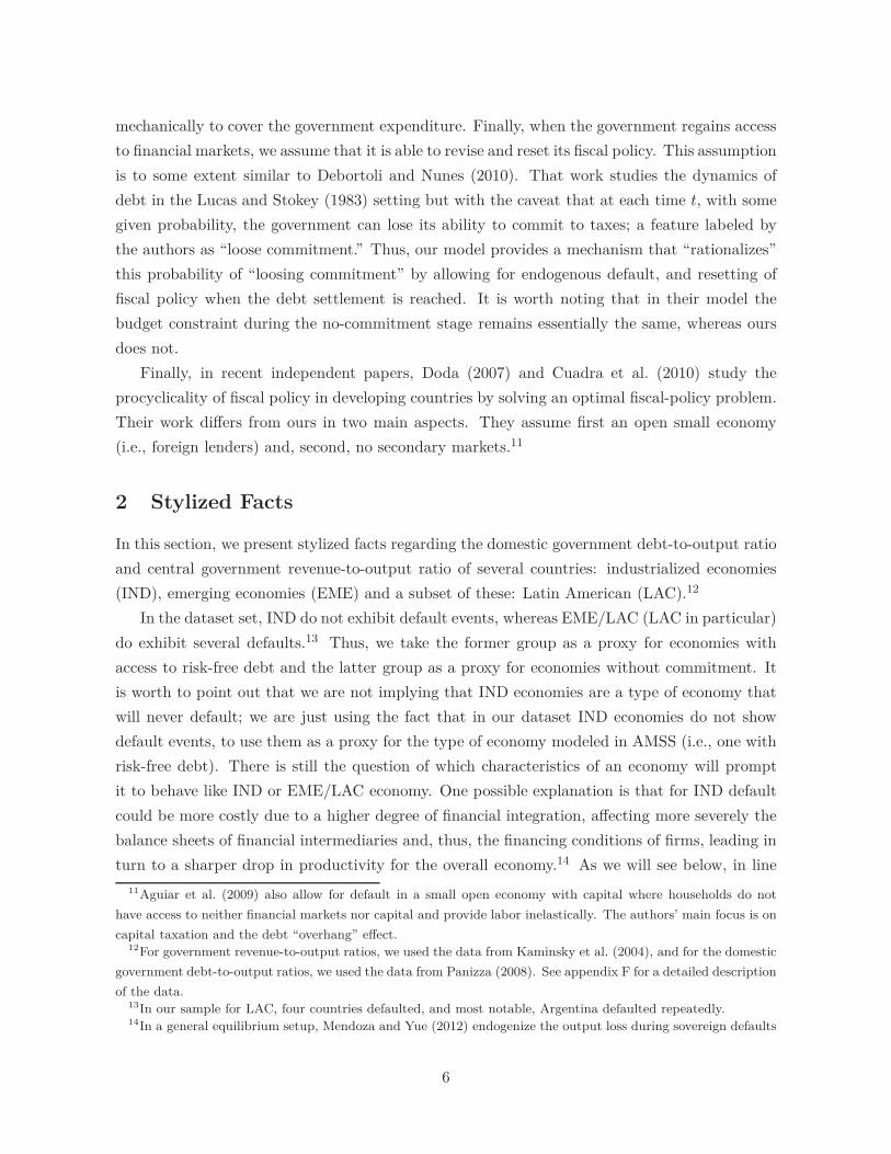
Figure 2.1 plots the percentiles of the domestic government debt-to-output ratio and of a

measure of default risk for three groups: IND (black triangle), EME (blue square) and LAC (red

circle).16 The X-axis plots the time series averages of domestic government debt-to-output ratio,

and the Y-axis plots the values of the measure of default risk.17 For each group, the last point

on the right correspond to the 95 percentile, the second to last to the 90 percentile and so on;

these are comparable between groups as all of them represent a percentile of the corresponding

distribution. EME and LAC have lower domestic debt-to-output ratio levels than IND; in fact

the domestic debt-to-output ratio value that amounts for the 95 percentile for EME and LAC,

only amounts for roughly 85 percentile for IND (which in both cases is only about 50 percent

as an outcome resulting from the substitution of imported inputs by less-efficient domestic ones when the financing

costs of the former rises due to sovereign default risk.15We refer the reader to Koenker (2005) for a thorough treatment of quantiles and quantile-based econometric

models.16This type of graph is not the conventional QQplot as the axis have the value of the random variable which

achieves a certain quantile and not the quantile itself. For our purposes, this representation is more convenient.17The measure of default risk is constructed as the spread using the EMBI+ real index from J.P. Morgan for

countries for which it is available and using the 3-7 year real government bond yield for the rest, minus U.S.

bond return. Although bond returns are not entirely driven by default risk but also capture other factors related

to risk appetite, uncertainty and liquidity, for our purpose they constitute a valid conventional proxy of default

risk. Furthermore, our spreads are an imperfect measure of default risk for domestic debt since EMBI+ considers

mainly foreign debt. However, it is still informative since domestic default are positively correlated with defaults

on sovereign debt, at least for the period of 1950’s onwards, see figure 10 in Reinhart and Rogoff (2008).

7

0 10 20 30 40 50 60 70 80 900

5

10

15

20

25

Debt/GDP

Defa

ult R

isk M

easu

re

95%

95%

95%

85%

← 50%

50% →

LACEMEIND

Figure 2.1: The percentiles of the domestic government debt-to-output ratio and of a measure

of default risk for three groups: IND (black triangle), EME (blue square) and LAC (red circle)

of debt-to-output ratio).18 Thus, economies that are prone to default (EME and LAC) exhibit

tighter debt ceilings than economies that do not default (in this dataset, represented by IND).

Figure 2.1 also shows that for the IND group, the default risk measure is low and roughly

constant for different levels of debt-to-output ratios. On the other hand, the default risk measure

for the EME group is not only higher, but increases substantially for high levels of debt-to-

output ratios. We consider this as evidence that, for EME economies, higher default risk is

more prevalent for high levels of debt-to-output ratios.

Table 2.1: (A) Measure of default risk (%) for EME and IND groups for different levels of debt-

to-output ratio (%); (B) standard deviation of central government revenue over GDP (%) for

EME and IND groups for different levels of default risk.

(A) (B)

Debt/GDP EME IND Default Risk EME IND

25 5.4 2.0 25 0.9 1.4

75 10.7 2.9 75 2.5 1.7

Table 2(A) compares the measure of default risk between IND and EME matching them

across low and high debt-to-output ratio levels. That is, for both groups (IND and EME)

18We obtain this by projecting the 95 percentile point of the EME and LAC onto the X-axis and comparing

with the 85 percentile point of IND.

8

we select economies with debt-to-output ratio below the 25th percentile (these are economies

with low debt-to-output) and for these economies we compute the average risk measure; we do

the same for those economies with debt-to-output ratio above the 75th percentile (these are

economies with high debt-to-output). For the case of low debt-to-output ratio, the EME group

presents higher (approximately twice as high) default risk than the IND group; however, for high

debt-to-output ratio economies, this difference is quadrupled. Thus, economies that are prone

to default (EME and LAC) exhibit higher default risk than economies that do not default (in

this dataset, represented by IND), and, moreover, the default risk is much higher for economies

in the former group that have high levels of debt-to-output ratio.

Table 2(B) compares the standard deviation of the central government revenue-to-output

ratio between IND and EME matching them across low and high default risk levels. It shows

that for IND there is little variation of the volatility across low and high levels of default risk.

For EME, however, the standard deviation of the central government revenue-to-output ratio is

higher for economies with high default risk.19 It is worth noting that all the EME with high

default risk levels defaulted at least once during our sample. Thus, economies with higher default

risk exhibit more volatile tax revenues than economies with low default risk. This is particularly

notable for the group of EME/LAC economies.

These stylized facts establish a link between (a) default risk/default events, (b) debt ceilings

and (c) volatility of tax revenues. In particular, the evidence suggests that economies that show

higher default risk, also exhibit lower debt ceilings and more volatile tax revenues. The theory

below sheds light upon the forces driving these facts.20

3 The Economy

In this section we describe the stochastic structure of the model, the timing and policies of the

government and present the household’s problem.

3.1 The Setting

Let time be indexed as t = 0, 1, .... Let (gt, δt) be the vector of government expenditure at time

t and the fraction of the defaulted debt which is to be repaid when exiting autarky, respectively.

If the economy is not in financial autarky, δt is equal to one in order to model the option of

the government to repay the totality of the debt or to default. These are the exogenous driving

random variables of this economy. Let ωt ≡ (gt, δt) ∈ G×∆, where G ⊂ R, ∆ ≡ ∆∪1∪δ and

∆ ⊂ [0, 1), and in order to avoid technical difficulties, we assume |G| and |∆| are finite.21 The

19We looked also at the inflation tax as a proxy for tax policy; results are qualitatively the same.20It is important to note that we are not arguing any type of causality; we are just illustrating co-movements.

In fact, in the model below all three features are endogenous outcomes of equilibrium.21For a given set, |S| is the cardinal of the set.

9

set ∆ models the offers — as fractions of outstanding debt — to repay the defaulted debt; and

δ is designed to capture situations where the government does not receive any offer to repay.22

For any t ∈ 1, ...., ∞, let Ωt = (G × ∆)t be the space of histories of exogenous shocks up

to time t, a typical element is ωt = (ω0, ω1, ..., ωt).

3.2 The government policies and timing

In this economy, the government finances exogenous government expenditures by levying labor

distortionary taxes and trading one-period, discount bonds with households. The government,

however, cannot commit to repay and may default on the bonds at any point in time.

Let B ⊆ R be compact. Let Bt+1 ∈ B be the quantity of bonds issued at time t to be paid

at time t + 1; Bt+1 > 0 means that the government is borrowing at time t from households.

Let τt be the linear labor tax. Also, let dt be the default decision, which takes value 1 if the

government decides to default and 0 otherwise. Finally, let at be the decision of accepting an

offer to repay the defaulted debt. It takes value 1 if the offer is accepted and 0 otherwise.

Also, for any t, let φt be the variable that takes value 0 if at time t the government cannot

issue bonds during this period, and value 1 if it can. The implied law of motion for φt is

φt ≡ φt−1(1 − dt) + (1 − φt−1)at. That is, if at time t − 1, the government could issue bonds,

then φt = (1 − dt), but if it was in financial autarky, then φt = at, reflecting the fact that the

government regains access to financial markets only if the government decides to renegotiate the

defaulted debt.

The timing for the government is as follows. Following a period with financial access, after

observing the current government expenditure, the government has the option to default on 100

percent of the outstanding debt carried from last period, Bt.

As shown in figure 3.2, if the government opts to exercise the option to default at time

t, it cannot issue bonds in that period and runs a balanced budget, i.e., tax revenues equal

government expenditure. At the beginning of next period, time t+1, with probability 1−λ, the

government remains in temporary financial autarky for that period (node B). With probability

λ, the government receives a random offer to repay a fraction δ of the debt, and has the option

to accept or reject it. If the government accepts the offer, it pays the restructured amount

(the outstanding defaulted debt times the fraction δ), and it is able to issue new bonds for the

following period (node A). If the government rejects the offer, it stays in temporary financial

autarky (node B).

Finally, if the government decides not to default, it levies distortionary labor taxes, and

allocates discount bonds to the households to cover the expenses gt and liabilities carried from

22An alternative way of modeling this situation is to work with ∆ ≡ ∆ ∪ 1 ∪ ∅ where ∅ indicates no

offer. Another alternative way is to add an additional random variable, ι ∈ 0, 1 that explicitly indicates if the

government received an offer (ι = 1) or not (ι = 0) and let ∆ ≡ ∆ ∪ 1.

10

t t

r

♦

s

♦♣②

♥ r

r

P

❯❱❲❳❨

❩ ❬❯ ❳

❭❪

Figure 3.2: Timing of the Model

last period. Next period, it has again the option to default, for the new values of outstanding

debt and government expenditure (node A).

As it will become clear later, default on bonds can be seen as a negative lump-sum transfer

to households, but a costly one. Default will turn to be costly for two reasons. First, house-

holds anticipate the government default strategies and demand higher returns to bear the bond.

Second, default is assumed to be followed by temporary financial autarky. During autarky, the

government is not only unable to issue debt but also could suffer an ad-hoc output cost, as

shown later.

We now formalize the probability model. Let πG : G → P(G) be the Markov transition

probability function for the process of government expenditures and let π∆ ∈ P(∆) be the

probability measure over the offer space ∆.23

Assumption 3.1. For any (t, ωt), Pr(gt = g|ωt−1) = πG(g|gt−1) for any g ∈ G and

Pr(δt = δ|gt, ωt−1) =

11(δ) if φt−1 = 1

(1 − λ)1δ(δ) + λπ∆(δ) if φt−1 = 0

for any δ ∈ ∆.24

23For a finite set X, P(X) is the space of all probability measures defined over X. Also, for any A ⊆ X, the

function 1A(·) takes value 1 over the set A and 0 otherwise.24It is easy to generalize this to a more general formulation such as λ and π∆ depending on g. For instance, we

11

Essentially, this assumption imposes a Markov restriction on the probability distribution

over government expenditures and also additional restrictions over the probability of offers. In

particular, this assumption implies that in financial autarky with probability 1 − λ, δ = δ (i.e.,

receiving no offer) and with probability λ, an offer from the offer space is drawn according to

π∆. Also, if φt−1 = 1 (i.e., the government was not in financial autarky at period t − 1), then

δt = 1 with probability one, which implies that if the government decides not to default at time

t, it will pay the totality of the outstanding debt.

Finally, we use Π to denote the probability distribution over Ω∞ generated by assumption

3.1, and Π(·|ωt) to denote the conditional probability over Ω, given ωt.

The next definitions formalize the concepts of government policy, allocation, prices of bonds

and the government budget constraint. In particular, it formally introduces the fact that taxes,

default decisions and debt depend on histories of past realizations of shocks, and in particular

that debt is non-state contingent (i.e., Bt+1 only depends on the history up to time t, ωt).

Definition 3.1. A government policy is a collection of stochastic processes σ = (Bt+1, τt, dt, at)∞t=0,

such that for each t, (Bt+1, τt, dt, at) ∈ B × [0, 1] × 0, 12 are measurable with respect to ωt and

(B0, φ−1).

Definition 3.2. An allocation is a collection of stochastic processes (gt, ct, nt)∞t=0 such that for

each t, (gt, ct, nt) ∈ G × R+ × [0, 1] are measurable with respect to ωt and (B0, φ−1).

Given a government policy, we say an allocation is feasible if for any (t, ωt)

ct(ωt) + gt = κt(ω

t)nt(ωt), (3.1)

where κt : Ωt → R+ is such that κt(ωt) is the productivity at period t, given history ωt. For

simplicity, we set κt(ωt) = φt(ω

t) + κ(1 − φt(ωt)) with κ ∈ (0, 1]. The parameter κ represents

direct output loss following a default event, associated for example with financial disruption in

the banking sector, limited insurance against idiosyncratic risk, among others.

Definition 3.3. A price process is an stochastic process (pt)∞t=0 such that for each t, pt ∈ R+ is

measurable with respect to ωt and (B0, φ−1).

Note that pt denotes the price of one unit of debt in any state of the world, both with

access to financial markets and during autarky, where it represents the price of defaulted debt

in secondary markets. Finally, we introduce the government budget constraint.

Definition 3.4 (def:sig-att). A government policy σ is attainable, if for all (t, ωt),

gt + φt(ωt)δtBt(ω

t−1) ≤ κt(ωt)τt(ω

t)nt(ωt) + φt(ω

t)pt(ωt)Bt+1(ωt), (3.2)

could allow for, say, π∆(·|gt, Bt, dt, dt−1, ..., dt−K) some K > 0, denoting that possible partial payments depend

on the credit history and level of debt. See Reinhart et al. (2003), Reinhart and Rogoff (2008) and Yue (2010)

for an intuition behind this structure.

12

and dt(ωt) = 1 if φt−1(ωt−1) = 0 and at(ω

t) = 0 if φt−1(ωt−1) = 1 or δt = δ. 25

Observe that in equation 3.2, if the government is in financial autarky (φt(ωt) = 0), its

budget constraint boils down to gt ≤ κt(ωt)τt(ω

t)nt(ωt). On the other hand, if the government

has access to financial markets (φt(ωt) = 1), then it has liabilities to be repaid for δtBt and can

issue new debt.26 The final restriction on dt(ωt) and at(ω

t) simply states that if last period the

government was in financial autarky, then it trivially cannot choose to default at time t, and if

δt = δ or if last period the government had access to financial markets at(ωt) is set to 0.

A few final remarks about the “debt-restructuring process” are in order. This process is

parameterized by (λ, π∆). These parameters capture the fact that debt restructuring is time-

consuming but, generally, at the end a positive fraction of the defaulted debt is honored.This

debt-restructuring process intends to capture the fact that after defaults (on domestic or inter-

national debt, or both), economies see their access to credit severely hindered.27

3.3 The Household’s Problem

There is a continuum of identical households, that are price takers and have time-separable

preferences for consumption and labor processes. They also make debt/savings decisions by

trading government bonds. Formally, we define a household debt process as a stochastic process

given by (bt+1)∞t=0 where bt+1 : Ωt → [b, b] is the household’s savings in government bonds at

time t + 1 for any history ωt.28

For convenience, let qt denote the price of defaulted debt at time t, i.e., qt = pt if φt = 0.

Given a government policy σ, for each t, let t : Ωt → R be the payoff of a government bond at

period t; i.e.,

t(ωt) = φt(ω

t)δt + (1 − φt(ωt))qt(ω

t). (3.3)

A few remarks about are in order. First, since the household takes government actions

as given, from the point of view of the households the government debt is an asset with payoff

that depends only on the state of the economy, and this dependence clearly illustrates that

25The inequality in equation 3.2 implies that the government can issue lump-sum transfers to the households.

Lump-sum taxes are not permitted.26If the government had access to financial markets at time t − 1 (φt−1 = 1), then by assumption 3.1, δt = 1

and the outstanding debt if simply Bt.27The duration of debt restructuring after sovereign defaults in particular on external debt has received consid-

erable attention in the literature. For instance, for Argentina’s default in 2001 the settlement with the majority of

the creditors was reached in 2005. In the default episodes of Russia (1998), Ecuador (1999) and Ukraine (1998),

the renegotiation process lasted 2.3, 1.7 and 1.4 years, respectively, according to Benjamin and Wright (2009). In

general, domestic debt restructuring periods tend to be not as long as in the case of external debt. For example,

as documented by Sturzenegger and Zettelmeyer (2006), after the default by Russia in 1998 it took six months

to restructure the domestic GKO bonds.28We assume bt+1 ∈ [b, b] with [b, b] ⊃ B so in equilibrium these restrictions will not be binding.

13

default decisions add certain degree of state contingency to the government debt. In particular,

if φt(ωt) = 1, then t(ω

t) = δt denoting the fact that the government pays a fraction δt. If

the government defaults or rejects the repayment option, the household can sell each unit of

government debt in the secondary market at a price t(ωt) = qt(ω

t).

The household’s problem consists of choosing consumption, labor and debt processes in order

to maximize the expected lifetime utility. That is, given (ω0, b0) and σ,

sup(ct,nt,bt+1)∞

t=0∈C(g0,b0;σ)EΠ(·|ω0)

[∞∑

t=0

βtu(ct(ωt), 1 − nt(ω

t))

]

where β ∈ (0, 1) is the discount factor, EΠ(·|ω0)[·] is the expectation using the conditional prob-

ability Π(·|ω0), and C(g0, b0; σ) is the set of household’s allocations and debt process, given

government policy σ, such that for all t and all ωt ∈ Ωt,

ct(ωt) + pt(ω

t)bt+1(ωt) = (1 − τt(ωt))κt(ω

t)nt(ωt) + t(ω

t)bt(ωt−1) + Tt(ω

t),

where Tt(ωt) ≥ 0 are lump-sum transfers from the government. The previous equation indicates

that after-tax labor income, proceedings from bond holdings and government transfers have to

be sufficient to cover consumption and new purchases of government bonds.

4 Competitive Equilibrium

We now define a competitive equilibrium for a given government policy and derive the equilib-

rium taxes and prices.

Definition 4.1. Given ω0, B0 = b0 and φ−1, a competitive equilibrium is a government policy,

σ, an allocation, (gt, ct, nt)∞t=0, a household debt process, (bt+1)∞

t=0, and a price process (pt)∞t=0

such that:

1. Given the government policy and the price process, the allocation and debt process solve

the household’s problem.

2. The government policy, σ, is attainable.

3. Given σ, the allocation is feasible.

4. For all (t, ωt), Bt+1(ωt) = bt+1(ωt), and Bt+1(ωt) = Bt(ωt−1) if φt(ω

t) = 0.

Observe that the market clearing for debt indicates that Bt+1(ωt) = bt+1(ωt). In addition, if

the economy is in financial autarky — where the government cannot issue debt, and thus agents

can only trade among themselves —, imposing Bt+1(ωt) = Bt(ωt−1) implies, since agents are

identical, that in equilibrium bt(ωt−1) = bt+1(ωt), i.e., agents do not change their debt positions.

14

4.1 Equilibrium Prices and Taxes

In this section we present the expressions for equilibrium taxes and prices of debt. The former

quantity is standard (e.g. Aiyagari et al. (2002) and Lucas and Stokey (1983)); the latter

quantity, however, incorporates the possibility of default of the government. The following

assumption is standard and ensures that u is smooth enough to compute first order conditions.

Assumption 4.1. u ∈ C2(R+ × [0, 1],R) with uc > 0, ucc < 0, ul > 0 and ull > 0, and

liml→0 ul(l) = ∞.29

Henceforth, for any (t, ωt), we use uc(ωt) as uc(ct(ω

t), 1 − nt(ωt)) and proceed similarly for

other derivatives and functions.

From the first order conditions of the optimization problem of the households (assuming an

interior solution) the following equations hold for any (t, ωt),30

ul(ωt)

uc(ωt)= (1 − τt(ω

t))κt(ωt), (4.4)

and

pt(ωt) =EΠ(·|ωt)

[β

uc(ωt+1)

uc(ωt)t+1(ωt+1)

]

=βEΠ(·|ωt)

[uc(ω

t+1)

uc(ωt)φt+1(ωt+1)δt+1

]+ βEΠ(·|ωt)

[uc(ω

t+1)

uc(ωt)(1 − φt+1(ωt+1))qt+1(ωt+1)

]

(4.5)

Given the definition of and the restrictions on Π, equation 4.5 implies for φt(ωt) = 1, 31

pt(ωt) =β

∫

G

(uc(ω

t, g′, 1)

uc(ωt)(1 − dt+1(ωt, g′, 1))

)πG(dg′|gt)

+ β

∫

G

uc(ωt, g′, 1)

uc(ωt)dt+1(ωt, g′, 1)qt+1(ωt, g′)πG(dg′|gt), (4.6)

and for φt(ωt) = 0 32

qt(ωt) =βλ

∫

G

∫

∆

(uc(ω

t, g′, δ′)

uc(ωt)δ′at+1(ωt, g′, δ′)

)π∆(dδ′)πG(dg′|gt)

+ βλ

∫

G

∫

∆

(uc(ω

t, g′, δ′)

uc(ωt)(1 − at+1(ωt, g′, δ′))π∆(dδ′)

)qt+1(ωt, g′)πG(dg′|gt)

+ β(1 − λ)

∫

G

(uc(ω

t, g′, δ)

uc(ωt)

)qt+1(ωt, g′)πG(dg′|gt). (4.7)

29C

2(X, Y ) is the space of twice continuously differentiable functions from X to Y . The assumption ucc < 0

could be relaxed to include ucc = 0 (see the section 6 below).30See appendix B for the derivation.31The notation (ωt, g, δ) denotes the partial history ωt+1 where (gt+1, δt+1) = (g, δ).32As it will become clear below, the price qt does not depend on δt, so we omit it from the notation.

15

Equation 4.5 reflects the fact that, in equilibrium, households anticipate the default strategies

of the government and demand higher returns to compensate for the default risk. The second line

in the Euler equation 4.6 shows that, due to the possibility of partial repayments in the future,

defaulted debt has positive value and agents can sell it in a secondary market at price qt+1(ωt+1).

Equation 4.7 characterizes this price. Each summand in the right hand side corresponds to a

“branch” of the tree depicted in figure 3.2. The first line represents the value of one unit of

debt when an offer arrives and the government decides to repay the realized fraction of the

defaulted debt next period. The second and third lines capture the value of one unit of debt

when either the government decides to reject the repayment offer, or it does not receive one.

A final observation is that, as it will become clear later on, when φt+1(ωt+1) = 0, uc(ωt+1) is

actually only a function of gt+1 (not the entire past history ωt+1) because in equilibrium the

government runs a balanced budget.

To shed some more light on equations 4.6 and 4.7, consider the case where uc = 1, λ = 0. In

this case, for any (t, ω)

pt(ω) = β

∫

G

(1 − dt+1(ωt, g′))πG(dg′|gt).

Also observe that, since λ = 0, it follows that qt(ωt) =

∫G

qt+1(ωt, g′)πG(dg′|gt), which by

substituting forward and invoking standard transversality conditions, yields qt(ωt) = 0. Thus,

the bond price pt, is simply the discounted one-period ahead probability of not defaulting. These

pricing equations are analogous to those in Arellano (2008) and Aguiar and Gopinath (2006)

and references therein. See also Chatterjee and Eyingungor (2012) for the equilibrium prices in

the presence of long-term debt.

The novelty of these pricing equations with respect to the standard sovereign default model

is the presence of secondary market prices, qt. By imposing a positive recovery rate (with some

probability), the model is able to deliver a positive price of defaulted debt during the financial

autarky period. In sections 6 and 7, we shed some light on the pricing implications of this model

and how it relates with the data.

4.2 Characterization of the Competitive Equilibrium

In this environment, the set of competitive equilibria can be characterized by a sequence of non-

linear equations which impose restrictions on (dt, at, Bt+1, nt)∞t=0 and are derived from the first

order conditions of the household, the budget constraint of the government and the feasibility

condition. The next theorem formalizes this claim.

Henceforth, we call (dt, at, Bt+1, nt)∞t=0 an outcome path of allocations. We say an outcome

path is consistent with a competitive equilibrium if the outcome path and (ct, pt, bt+1, τt, gt)∞t=0,

derived using the market clearing, feasibility and first order conditions, is a competitive equilib-

16

rium. Also, let

Zt(ωt) ≡ z(κt(ω

t), nt(ωt), gt) =

(κt(ω

t) −ul(ω

t)

uc(ωt)

)nt(ω

t) − gt (4.8)

be the primary surplus (if it is negative, it represents a deficit) at time t given history ωt ∈ Ωt.

Theorem 4.1. Given ω0, B0 = b0 and φ−1, the outcome path (dt, at, Bt+1, nt)∞t=0 is consistent

with a competitive equilibrium iff for all (t, ωt) ∈ 0, 1, 2, ... × Ωt, the following holds:

Zt(ωt)uc(ω

t) + φt(ωt)pt(ω

t)uc(ωt)Bt+1(ωt) − δtuc(ω

t)Bt(ωt−1) ≥ 0, (4.9)

Bt+1(ωt) = Bt(ωt−1) if φt(ω

t) = 0,

and ct(ωt) = κt(ω

t)nt(ωt) − gt(ω

t) and equations 4.4 and 4.6 hold.

For any (ω, B, φ) ∈ (G× ∆) ×B× 0, 1, let CEφ(ω, B) denote the set of all outcome paths

that are consistent with competitive equilibria, given ω0 = ω, φ0(ω0) = φ and where B is the

outstanding debt of time 0, after any potential debt restructuring in that period.33 We observe

that by setting φ0(ω0) = φ we are implicitly imposing restrictions on a0, d0, φ−1 and δ0.34

Equation 4.9 summarizes the budget constraint of the government but replacing prices and

taxes by the first order conditions, as in the ”primal approach” used by Lucas and Stokey (1983)

and Aiyagari et al. (2002).

5 The Government Problem

The government is benevolent and maximizes the welfare of the representative household by

choosing policies. The government, however, cannot commit to repaying the debt, but commits

to previous tax promises until a debt restructuring takes place. That is, as long as the government

keeps access to financial markets, it honors past promises of taxes. This assumption facilitates

the comparison to the optimal taxation literature in the spirit of Lucas and Stokey (1983) and

Aiyagari et al. (2002).

For autarky states, the government chooses taxes that balance its budget. Once the govern-

ment accepts an offer to restructure the debt, it regains access to financial markets and starts

anew, without any outstanding tax promises, by assumption. A similar feature is present in

Debortoli and Nunes (2010), where the government can randomly re-optimize and reset fiscal

policies with a given exogenous probability.35

33Constructing the set CEφ(ω, B) is useful since, in order to make a default/repayment decision, the default

authority evaluates alternative utility values both for repayment and for autarky that are sustained by competitive

equilibrium allocations.34For example, if φ0 = 1 we could only arrive to it because either φ−1 = 1 and d0 = 0, given (g0, B0) = (g, B),

or because φ−1 = 0 with defaulted debt B0 = B0/δ0 – and offer δ0 is accepted (a0 = 1).35In our model, however, the resetting event, given by the debt restructuring, is an equilibrium outcome that

emerges endogenously.

17

The government problem can thus be viewed as a problem involving two types of authorities:

a default authority and a fiscal authority. On the one hand, the default authority can be seen as

comprised by a sequence of one-period administrations, where the time-t administration makes

the default and repayment decision in period t, taking as given the behavior of all the other

agents including the fiscal authority. On the other hand, the fiscal authority can be viewed as

a sequence of consecutive administrations, each of which stays in office until there is a debt

renegotiation. While ruling, a fiscal administration has the ability to commit, and chooses the

optimal fiscal and debt processes, taking as given the behavior of the default authority. When

debt is renegotiated, the fiscal administration is replaced by a new one, which is not bound by

previous tax promises, and is free to reset the fiscal and debt policy.36

5.1 The Government Policies

For any t ∈ 0, 1, ..., let ht ≡ (φt−1, Bt, ωt) and ht ≡ (h0, h1, ...., ht) be the public history until

time t.37 We use Ht to denote the set of all public histories until time t.

A government strategy is given by a strategy for the default and fiscal authorities, γ ≡

(γD, γF ). The strategy for the default authority γ

D specifies a default and a repayment de-

cision for any period t and any public history ht ∈ Ht, i.e., γ

D = (γDt (·))∞

t=0 with γDt (ht) ≡

(dt(ht), at(h

t)) for any ht ∈ Ht. The strategy for the fiscal authority, γ

F , specifies next pe-

riod’s debt level for any public history ht ∈ Ht and any φt, i.e., γ

F = (γFt (·, ·))∞

t=0 with

γFt (ht, φt) ≡ Bt+1(ht, φt) for any (ht, φt) ∈ H

t × 0, 1. The fact that γFt (ht, φt) depends on

φt reflects our assumption on the timing protocol by which the default authority moves first in

each period.38 Finally, note that any strategy γ jointly with (ωt)∞t=0 generates an outcome path

of allocations (dt, at, Bt+1, nt)∞t=0. To stress that a particular policy action, say Bt+1(ht, φt),

belongs to a given strategy we use Bt+1(γ)(ht, φt).

Let γ|(ht,φt) denote the continuation of strategy γ after history (ht, φt) ∈ Ht × 0, 1.39 We

say a strategy γ is consistent with a competitive equilibrium, if after any (ht, φt) ∈ Ht × 0, 1,

36We focus exclusively on symmetric strategies for households, where all of them take the same decisions along

the equilibrium path. Similarly, we assume that all default and fiscal administrations choose identical actions

conditional on the same state of the economy, thereby introducing a Markovian structure for optimal strategies.37In our economy an individual household cannot alter prices and faces a (strictly) concave optimization prob-

lem. Any deviation from the equilibrium path determined by the Euler equation and the consumption-labor

optimality condition, taking prices and policies as given, cannot be profitable from the household’s perspective.

Hence, there is no need to specify the household’s behavior off the equilibrium path as well as to make households’

strategies depend on private histories but only on public ones.38We omit labor taxes (or labor directly) as part of the government strategy because, given (ht, φt) and

γFt (ht, φt), labor taxes are obtained by the budget constraint. For this reason we do not include them as part of

the public history.39Observe that while a strategy prescribes that the default authority moves first at t = 0, with the continuation

strategy, as we defined, the fiscal authority is moving first at t and then the default authority moves at t + 1.

18

the outcome path generated by γ|(ht,φt) belongs to CEφt(ωt, B) with outstanding debt B =

(δtφt + (1 − φt))Bt(γ)(ht−1, φt−1(γ)(ht−1)). That is, if there is full repayment (i.e. no default)

or not borrowing at all in the current period t, the debt level B is given by the bond holdings

carried over from last period. Otherwise, if the government just regained access by accepting

an offer δt, B is the restructured debt level.

For any h0 ∈ H and φ0 ∈ 0, 1, we use S(h0, φ0) to denote the set of such strategies; see

Appendix D for the formal expression of S(h0, φ0). Henceforth, we only consider strategies that

are consistent with competitive equilibrium.

Finally, for any public history ht ∈ Ht, φ ∈ 0, 1 and γ ∈ S(h0, φ), let

Vt(γ)(ht, φ) = EΠ(·|ωt)

∞∑

j=0

βju(κt+j(ωt+j)nt+j(γ)(ωt+j) − gt+j , 1 − nt+j(γ)(ωt+j))

(5.10)

be the expected lifetime utility of the representative household at time t, given strategy γ|(ht,φ).

5.2 Default and Renegotiation Policies

As mentioned before, the default authority can be viewed as comprised by a sequence of one-

period administrations, each of which makes the default and renegotiation decision in its re-

spective period, taking as given the behavior of all the other agents including the other default

and fiscal administrations. It is easy to see that, for each public history ht ∈ Ht, the default

authority will optimally choose as follows: if φt−1 = 1

d∗t (γ)(ht) =

0 if Vt(γ)(ht, 1) ≥ Vt(γ)(ht, 0)

1 if Vt(γ)(ht, 1) < Vt(γ)(ht, 0)(5.11)

and if φt−1 = 0

a∗t (γ)(ht) =

1 if Vt(γ)(ht, 1) ≥ Vt(γ)(ht, 0)

0 if Vt(γ)(ht, 1) < Vt(γ)(ht, 0)(5.12)

The dependence on γ denotes the fact that d∗t and a∗

t are associated with the strategy of the

fiscal authority γF . Indeed, to specify the optimal default and repayment decisions at any

history ht ∈ Ht we need to know the value of repayment and the value of default, Vt(γ)(ht, 1)

and Vt(γ)(ht, 0), respectively, which are evidently functions of γF .40

5.3 Recursive Representation of the Government Problem

Taking as given the optimal decision rules 5.11 and 5.12 for the default authority, we now

turn to the optimization problem of the fiscal authority and the recursive representation of the

40Also, recall that by assumption a∗t (γ)(ht) = 0 if φt−1 = 1 or δt = δ and d∗

t (γ)(ht) = 1 if φt−1 = 0.

19

government problem. To do so, we adopt a recursive representation for the competitive equilibria

by introducing an adequate state variable. Following Kydland and Prescott (1980) and Chang

(1998) among others, it follows that the relevant (co-)state variable is the “promised” marginal

utilities of consumption.41

For any h0 = (φ−1, B0, g0, δ0) ∈ H and φ ∈ 0, 1, let Ω(h0, φ) be the set of all marginal

utility values (µ) and lifetime utilities at time zero (v) that can be sustained in a competitive

equilibrium, wherein the default authority reacts optimally from next period on; see Appendix

D for the formal expression of Ω(h0, φ).

It is worth to point out that this set differs from the standard set of equilibrium promised

marginal utilities in Kydland and Prescott (1980) along some dimensions. In particular, in an

standard Ramsey problem it would suffice to only specify the set of promised marginal utilities,

but in our framework with endogenous default decisions we find it convenient to also specify

continuation values to evaluate alternative courses of action of the default authority. By the

same token, we compute this set for any φ, even for the value of φ not optimally chosen by the

default authority through its policy action.

For any (g, B, µ) ∈ G×B×R+, let V ∗1 (g, B, µ) be the value of a fiscal authority that had access

to financial markets last period and continue to have it this current period (i.e., φ−1 = φ = 1)

and that takes as given the optimal behavior of the default and subsequent fiscal authorities,

with outstanding debt B and a promised marginal utility of µ and government expenditure g.

Similarly, let V ∗0 (g, B) be the value of a fiscal authority that does not have access to financial

markets (i.e., φ = 0). Observe that since in financial autarky the government ought to run a

balanced budget, V ∗0 does not depend on µ.

Finally, let V∗1(g, δB) be the value of a “new” fiscal authority (i.e., when φ−1 = 0 and φ = 1)

that takes as given the optimal behavior of the default and subsequent fiscal authorities, when

an offer δ is accepted, given government spending g and outstanding defaulted debt B. Note

that in this case the fiscal authority does not have any outstanding “promised” marginal utility

and thus it sets the current marginal utility at its convenience. By definition of Ω, it follows

that

V∗1(g, δB) = maxv|(µ, v) ∈ Ω(0, B, g, δ, 1), (5.13)

as the government maximizes the households’ utility without any attached promise of marginal

utility to be delivered.42 Let µ(g, δ, B) = µ|(µ, V∗1(g, δB)) ∈ Ω(0, B, g, δ, 1) be the associated

41By keeping track of the profile of “promised” marginal utilities of consumption, we ensure that the fiscal

authority commits to deliver the “promised” marginal utility —as long as the default authority does not restructure

the debt— for each realization of g; thereby guaranteeing that the last-period households’ Euler equation is

satisfied after each possible history. If the debt is restructured and a new fiscal administration takes power, it

sets the current marginal utility at its convenience, which in equilibrium is anticipated by the households.42We are implicitly assuming that the maximum is achieved. This assumption is imposed to ease the exposition

and could be relaxed by defining V∗1 in terms of a supremum and approximate maximizers.

20

marginal utility.

Given the aforementioned value functions, the optimal policy functions of the default au-

thority in expressions 5.11-5.12 become 43,44

d∗(g, B, µ) =

0 if V ∗1 (g, B, µ) ≥ V ∗

0 (g, B)

1 if V ∗1 (g, B, µ) < V ∗

0 (g, B)(5.14)

and

a∗(g, δ, B) =

1 if V∗1(g, δB) ≥ V ∗

0 (g, B)

0 if V∗1(g, δB) < V ∗

0 (g, B)(5.15)

The next theorem presents a recursive formulation for the value functions. In what follows,

we denote the marginal utility of consumption in financial autarky as mA(g) for all g ∈ G.45

Theorem 5.1. The value functions V ∗0 and V ∗

1 satisfy the following recursions

V ∗1 (g, B, µ) = max

(n,B′,µ′(·))∈Γ(g,B,µ)

u(n − g, 1 − n) + β

∫

G

maxV ∗1 (g′, B′, µ′(g′)), V ∗

0 (g′, B′)πG(dg′|g)

,

(5.16)

and

V ∗0 (g, B) =u(κn∗

0(g) − g, 1 − n∗0(g)) + βλ

∫

G

∫

∆maxV

∗1(g′, δ′B), V ∗

0 (g′, B)π∆(dδ′)πG(dg′|g)

+ β(1 − λ)

∫

G

V ∗0 (g′, B)πG(dg′|g) (5.17)

where, for any (g, B, µ),

Γ(g, B, µ) =

(n, B′, µ′(·)) ∈ [0, 1] × B × R|G| :

(B′, µ′(g′), V ∗1 (g′, B′, µ′(g′)) ∈ Graph(Ω(1, ·, g′, 1, 1)), ∀g′ ∈ G

µ = uc(n − g, 1 − n) and z(1, n, g)µ + P∗1 (g, B′, µ′(·))B′ − Bµ ≥ 0

(5.18)

and, for any (B′, µ′(·)),

P∗1 (g, B′, µ′(·)) =β

∫

G

((1 − d∗(g′, B′, µ′(g′)))µ′(g′) + d∗(g′, B′, µ′(g′))mA(g′)P∗

0 (g′, B′))

πG(dg′|g)

P∗0 (g, B′) =β

∫

G

(∫

∆µ(g′, δ′, B′)δ′a∗(g′, δ′, B′)π∆(dδ′) + π∗

A(g′, B′)mA(g′)P∗0 (g′, B′)

)πG(dg′|g)

where π∗A(g, B) ≡ (1 − λ) + λ

∫∆(1 − a∗(g, δ, B))π∆(dδ) for any (g, B).

43Implicit in both definitions is the refinement that in case of indifference, the government decides to accept/not

default on the debt. Without this refinement, the optimal decisions will be correspondences that take any value

between 0 and 1 in case of indifference.44As indicated before, by assumption, d

∗(g, B, µ) = 1 if φ−1 = 0 and a∗(g, δ, B) = 0 if φ−1 = 1 or δ = δ.

45Formally, mA(g) = uc(κn∗0(g) − g, 1 − n

∗0(g)) where n

∗0(g) = arg maxn∈[0,1]u(κn − g, 1 − n) : z(κ, n, g) = 0.

See appendix D for details.

21

Below we present some particular cases of special interest where the recursive representation

of the government problem gets simplified.

Example 5.1 (Nondefaultable debt). Consider an economy with risk-free debt (this is imposed

ad-hoc). The value function V ∗0 is irrelevant and V ∗

1 boils down to

V ∗1 (g, B, µ) = max

(n,B′,µ′(·))∈Γ(g,B,µ)

u(n − g, 1 − n) + β

∫

G

V ∗1 (g′, B′, µ′(g′))πG(dg′|g)

where

Γ(g, B, µ) =

(n, B′, µ′(·)) : z(1, n, g)µ + βEπG(·|g)[µ′(g′)]B′ − Bµ ≥ 0

where µ = uc(n − g, 1 − n)

.

In addition, since there is no “re-setting” time, V ∗1 coincides with the value function at time

0 with µ chosen optimally. This case is precisely the type of model studied in Aiyagari et al.

(2002).

Example 5.2 (quasi-linear per-period payoff, λ ≥ 0, and π∆ = 10). Assume that u(c, 1−n) =

c + H(1 − n) for some function H consistent with assumption 4.1. Under this assumption, µ

can be dropped as a state variable since uc = 1 and thus it does not affect the pricing equation.

In this case, the value function during financial autarky is given by

V ∗0 (g) =κn

∗0(g) − g + H(1 − n

∗0(g)) + β

∫

G

(λV ∗

1 (g′, 0) + (1 − λ)V ∗0 (g′)

)πG(dg′|g).

This expression follows from the fact that there is no need to keep the debt B as part of the state

during financial autarky since none of the defaulted debt is ever repaid, and all the offers of zero

repayment are accepted by the government. The value function during financial access is given

by

V ∗1 (g, B) = max

(n,B′)∈Γ(g,B)

n − g + H(1 − n) + β

∫

G

maxV ∗1 (g′, B′), V ∗

0 (g′)πG(dg′|g)

,

where Γ(g, B) ≡ (n, B′) : z(1, n, g) + βEπG(·|g)[1g′:V ∗1 (g′,B′)≥V ∗

0 (g′)(g′)]B′ − B ≥ 0.

The expression for the price function highlights an important difference between our default

model and a model with risk-free debt such as AMSS. Since uc = 1, the market stochastic discount

factor is equal to β, and thus in the AMSS model the government cannot manipulate the return

of the discount bond. In our economy with defaultable debt, however, while not being able to

influence the risk-free rate, the government is still able to manipulate the return of the discount

bond by altering its payoff through the decision of default.

Moreover, assuming H is increasing and strictly concave with H ′(1) < 1 and 2H ′′(l) <

H ′′′(l)(1 − l), we can view the government problem as directly choosing tax revenues R with a

per-period payoff given by Wκ(R) = κnκ(R) + H(1 − nκ(R)) where nκ(R) is the amount of labor

22

needed to collect revenues equal to R, given κ. Under our assumptions, Wκ is non-increasing

and concave function. The Bellman equation of the value of repayment is given by

V ∗1 (g, B) = max

(R,B′)

W1(R) − g + β

∫

G

maxV ∗1 (g′, B′), V ∗

0 (g′)πG(dg′|g)

, (5.19)

subject to R + βEπG(·|g)[1g′:V ∗1 (g′,B′)≥V ∗

0 (g′)(g′)]B′ ≥ g + B, and

V ∗0 (g) =Wκ(g) − g + β

∫

G

(λV ∗

1 (g′, 0) + (1 − λ)V ∗0 (g′)

)πG(dg′|g). (5.20)

The previous equations imply that this government’s problem is analogous to that studied in

Arellano (2008) and Aguiar and Gopinath (2006) among others, where the government chooses

how much to “consume”, captured by −R, given an exogenous process of “income”, −g. An

important difference, however, is the non-standard per-period payoff which reflects the distortive

nature of labor taxes. In particular in our model the per-period payoff has a satiation point at

R = 0 (i.e., zero distortive taxes).46

We think this last observation is relevant because it allows us to extend some of our results

to general sovereign debt models with endogenous default, especially those results regarding the

impact of the debt restructuring in debt prices (both, before and during financial autarky).

6 Analytical Results

In this section we present analytical results for a benchmark model characterized by quasi-linear

per-period utility, i.i.d. government expenditure shocks and debt repayments for exiting financial

autarky. The proofs for the results are gathered in appendix E.

Assumption 6.1. (i) κ = 1; (ii) u(c, n) = c+H(1−n) where H ∈ C2((0, 1),R) with H ′(0) = ∞,

H ′(l) > 0, H ′(1) < 1, H ′′(l) < 0 and 2H ′′(l) < H ′′′(l)(1 − l)

Part (i) implies that there are no direct cost of defaults in terms of output. Part (ii) of

this assumption imposes that the per-period utility of the households is quasi-linear and it is

analogous to assumption in p. 10 in AMSS. As noted above, under this assumption, µ can be

dropped as a state variable. This implies that the value functions V ∗0 , V ∗

1 are only functions of

(g, B) and the same holds true for the optimal policy functions.

We also assume that government expenditure are i.i.d., formally

Assumption 6.2. For any g′ 6= g, πG(·|g) = πG(·|g′).

46Another subtle difference with the standard sovereign default literature is that while in our economy govern-

ment and bondholders share the same preference, in this literature they do not. In particular, the government

tends to be more impatient than (foreign) investors, thus bringing about incentives to front-load consumption

through borrowing.

23

With a slight abuse of notation and to simplify the exposition we use πG(·) to denote the

probability measure of g. Finally, to further simplify the technical details, we assume that B

has only finitely many points, unless stated otherwise.47

For the rest of the section, we proceed as if these assumptions 6.1 - 6.2 hold and will not be

referenced explicitly.

6.1 Characterization of Optimal Default Decisions

The next proposition characterizes the optimal decisions to default and to accept offers to repay

the defaulted debt as “threshold decisions”. These results are analogous to Arellano (2008)

but extended to this setting, in particular we allow for partial repayments of government debt.

Recall that d∗(g, B) and a∗(g, δ, B) are the optimal decision of default and of renegotiation,

respectively, given the state (g, δ, B).

Proposition 6.1. There exists λ such that for all λ ∈ [0, λ], the following holds:

1. There exists a δ : G × B → ∆ such that a∗(g, δ, B) = 1δ:δ≤δ(g,B)(δ) and δ non-increasing

as a function of B.48

2. There exists a g : B → G such that d∗(g, B) = 1g:g≥g(B)(g) and g non-increasing for all

B > 0.

This result shows that for a (non-trivial) range of probabilities of receiving outside of-

fers, λ ∈ [0, λ], default is more likely to occur for high levels of debt, and so are rejections

of offers to exit financial autarky.49 The latter result implies that the average recovery rate,

EπG[∫

δ′∈∆ δ′1δ : δ≤δ(g,B)(δ′)π∆(dδ′)], is decreasing in the level of debt, as documented by Yue

(2010) in the data. It also follows that other things equal, higher debt levels are on average

associated with longer financial autarky periods. Thus, these two results imply a positive co-

movement between the (observed) average haircut and the average length of financial autarky.

This last fact seems to be consistent with the data; see fact 3 in Benjamin and Wright (2009).

Cruces and Trebesch (2013) found a similar relationship for 180 sovereign debt restructuring

cases of 68 countries between 1970 and 2010.50

47This assumption is made for simplicity. It can be relaxed to allow for general compact subsets, but some of

the arguments in the proofs will have to be changed slightly. Also, the fact that B ≡ B1, ..., B|B| is only imposed

for the government; the households can still choose from convex sets; only in equilibrium we impose B1, ..., B|B|.48It turns out that the first part of the statement holds for any λ.49The value of λ depends on the parametrization of the model. For instance, in our numerical simulations for

the benchmark calibration with λ = 0.2, all theoretical results from proposition 6.1 hold, therefore implying that

λ ≥ 0.2.50It is important to note, however, that we derived the implications by looking at exogenous variations of the

debt level; in the data this quantity is endogenous and, in particular, varies with g. This endogeneity issue

taken into account in the numerical simulations, wherein we perform a more thorough test of the aforementioned

implications.

24

6.2 Implications for Equilibrium Prices and Taxes

We now study the implications of the above results on equilibrium prices and taxes.

Equilibrium prices and endogenous debt limits. Under assumption 6.2 equilibrium

prices do not depend on g, i.e., P∗φ(·) ≡ P∗

φ(g, ·) for any g ∈ B. By proposition 6.1 it follows

that, for any B′ ∈ B,

P∗1 (B′) =β

∫

G

1g′≤g(B′)(g′)πG(dg′) +

(β

∫

G

1g′>g(B′)(g′)πG(dg′)

)P∗

0 (B′) (6.21)

and 51

P∗0 (B) =

βλ∫

∆

(∫G

1δ:δ≤δ(g′,B)(δ)πG(dg′))

δπ∆(dδ)

1 − β + βλ∫

∆

∫G

1δ:δ≤δ(g′,B)(δ)πG(dg′)π∆(dδ). (6.22)

A key feature of endogenous default models is the existence of endogenous borrowing limits.

A necessary condition for this result is that, due to the possibility of default, equilibrium prices

are non-increasing as a function of debt; thus implying a “Laffer-type curve” for the revenues

coming from selling bonds. In an economy without debt repayment (e.g., π∆ = 10), it fol-

lows that P∗0 = 0 and P∗

1 (B′) = β∫G

1g:g≤g(B′)(g′)πG(dg′) which is non-increasing in B′ by

proposition 6.1. Moreover, it takes value zero for sufficiently high B′. Therefore, there exists an

endogenous debt limit, i.e., finite value of B′ that maximize the debt revenue P∗1 (B′)B′.

In an economy where we allow for debt repayments, by inspection of equation 6.21 and the

fact that P∗0 ≥ 0, it is easy to see that, other things equal, the previous result is attenuated by the

presence of (potential) defaulted debt payments and secondary markets. The next proposition

shows that when repayment offers exist but are non-random, the price is non-increasing on the

level of debt and there are endogenous borrowing limits.

Proposition 6.2. Suppose π∆(·) = 1δ0(·) for some δ0 ∈ [0, 1]. Then there exists a λ > 0, such

that for all λ ∈ [0, λ], P∗i (·) is non-increasing for B > 0 and for i = 0, 1.

This proposition shows that high levels of debt are associated with higher return on debt,

both before and during financial autarky. This result is consistent with the evidence regarding

debt-to-output levels and default risk measures presented in section 2. Moreover, this result

in conjunction with the implications derived from proposition 6.1, implies that high levels of

debt are associated with higher return on debt, lower (observed) average recovery rate, and, on

average, longer financial autarky spells. In particular, it implies that (on average) longer periods

in financial autarky are associated with higher spreads during this period.

In addition, the existence of endogenous borrowing limits implies that the ability to roll over

high levels of debt is hindered. This in turn implies that due to the concavity of z(1, ·, g), labor

51See lemma E.5(3) in the appendix for the derivation.

25

is more “sensitive” to fluctuations in government expenditure. This fact relates to the stylized

fact regarding volatility of revenue-to-output ratios described in section 2; we further explore

this mechanism in the numerical simulations.

Default risk and the law of motion of equilibrium taxes. In order to analyze the ex-

ante effect of default risk on the law of motion of taxes, we consider the case λ = 0 (i.e., autarky

is an absorbing state) to simplify the analysis. We also strengthen assumption 6.1 by requiring

that H ′′(l) < H ′′′(l)(1− l). By proposition 6.1, the default decision is a threshold decision, so for

each history ω∞ ∈ Ω∞ we can define T (ω∞) = inft : gt ≥ g(Bt(ωt−1)) (it could be infinity) as

the first time the economy enters in default. For all t ≤ T (ω∞) the economy is not in financial

autarky, and the implementability constraint is given by

Bt(ωt−1) + gt ≤

(1 − H ′(1 − nt(ω

t)))

nt(ωt) + P∗

1 (Bt+1(ωt))Bt+1(ωt),

where P∗1 (gt, Bt+1(ωt)) ≡ EπG

[1 − d∗(g′, Bt+1(ωt))]. Let νt(ωt) be the Lagrange multiplier

associated to this restriction in the optimization problem of the government, given ωt ∈ Ωt. In

appendix E.2 we derive the FONC of the government and provide a closed form expression for

νt(ωt) as a decreasing nonlinear function of nt(ω

t); see equation E.87.52 Hence, as noted by

AMSS, by studying the law of motion of νt we can shed light on the law of motion of labor and

taxes.

From the FONC of the government it follows (see appendix E.2 for the derivation)53,54

νt(ωt)

(1 +

dP∗1 (Bt+1(ωt))

dBt+1

Bt+1(ωt)

P∗1 (Bt+1(ωt))

)=

∫

G

νt+1(ωt, g′)1g′ ≤ g(Bt+1(ωt))∫

G1g′ ≤ g(Bt+1(ωt))πG(dg′)

πG(dg′).

(6.23)

The Lagrange multiplier associated with the implementability condition is constant in Lucas

and Stokey (1983) and, thus, trivially a martingale. In Aiyagari et al. (2002) the Lagrange

multiplier associated with the implementability condition is a martingale with respect to the

probability measure πG. Equation 6.23 implies that the law of motion of the Lagrange multiplier

differs in two important aspects. First, the expectation is computed under the so-called default-

adjusted probability measure, given by 1·≤g(Bt+1(ωt))∫G

1g′≤g(Bt+1(ωt))πG(dg′)πG(·). The wedge between πG and

this new probability stems from the fact that the option to default adds “some” degree of state-

contingency to the payoff of the government debt making it lower for high values of government

52The strengthening of assumption 6.1 is only needed to show that νt(ωt) is an decreasing function of nt(ω

t);

the proof is in appendix E.2.53This derivation assumes that B is a convex set and πG has a density with respect to the Lebesgue measure,

so as to make sense of differentiation. It also assumes differentiability of V ∗.54The martingale property is also preserved if capital is added to the economy; see Farhi (2010). If we allow

for ad-hoc borrowing/savings limits, the equality has to be replaced by the corresponding inequality; see Aiyagari

et al. (2002).

26

expenditure, and implies that the default-adjusted probability measure is first order dominated

by πG. In fact, it implies that only the states tomorrow in which there is repayment, are relevant

for the law of motion of νt.55 It follows that, in the case that νt+1(ωt, ·) is increasing, the

presence of the default-adjusted probability lowers νt(ωt) and, consequently, lowers also the tax

distortions.56 Second, νt(ωt) in the left-hand side is multiplied by

(1 +

dP∗1 (Bt+1(ωt))

dBt+1

Bt+1(ωt)P∗

1 (Bt+1(ωt))

),

which can be interpreted as the “markup” that the government has to pay for having the option

to default; this effect increases νt(ωt) and the tax distortions. These two forces act in opposite

directions, and is not clear which one will prevail. In order to shed more light on this issue, in

section 7 we explore quantitatively this trade-off by plotting the impulse responses for νt(ωt)

delivered by our model and a version of Aiyagari et al. (2002).

7 Numerical Results

Throughout this section, we run a battery of numerical exercises in order to assess the perfor-

mance of the model and assess the capability of the model to quantitatively generate the stylized

facts discussed in section 2. We compare our findings with an economy in which the option to

default is not present—precisely the model considered in Aiyagari et al. (2002). We denote the

variables associated with this model with a (sub)superscript “AMSS”; variables associated to

our economy are denoted with a (sub)superscript “ED” (short for Economy with Default).

In the dataset IND economies are proxies of the AMSS model and EME/LAC are proxies

of our model. As discussed before, IND do not exhibit default events in the dataset. There

is the question of what characteristics of the economy will prompt it to behave like AMSS- or

ED-type economies. One possible explanation is that by factors unrelated to the model, such as

political instability, ED presents lower discount factor from the government and thus are more

prone to default. An alternative explanation, in line with our model, is that for AMSS-type/IND

economies, default is more costly because they are financially more integrated, and the financial

autarky following a default could have a larger impact on financing of the firms, thus lowering

their productivity (in our model represented by a lower κ).57

Benchmark Calibration. For all the simulations the utility function is given by u(c, 1 −

n) = c + C1(1−n)1−σ

1−σ, where −σ is the inverse Frisch elasticity of labor supply.58 In this

parametrization, we assume that |G| consists of five values, evenly spaced between [0.207, 0.277];

55If default occurs, the link between multipliers today and tomorrow is severed and tax rates stop exhibiting

persistence, as they are set to balance the budget inheriting the i.i.d. properties of the stochastic process of the

government spending.56By calculations in the Appendix E.2, νt+1(ωt, ·) is increasing iff n

∗1 is decreasing in g.

57In our calibration, κ = 0.96, is sufficiently low to prevent the economy from defaulting.58For this preference choice, it is easy to see that whether the fiscal authority has the ability to commit to tax

policies or not renders the same equilibrium results.

27

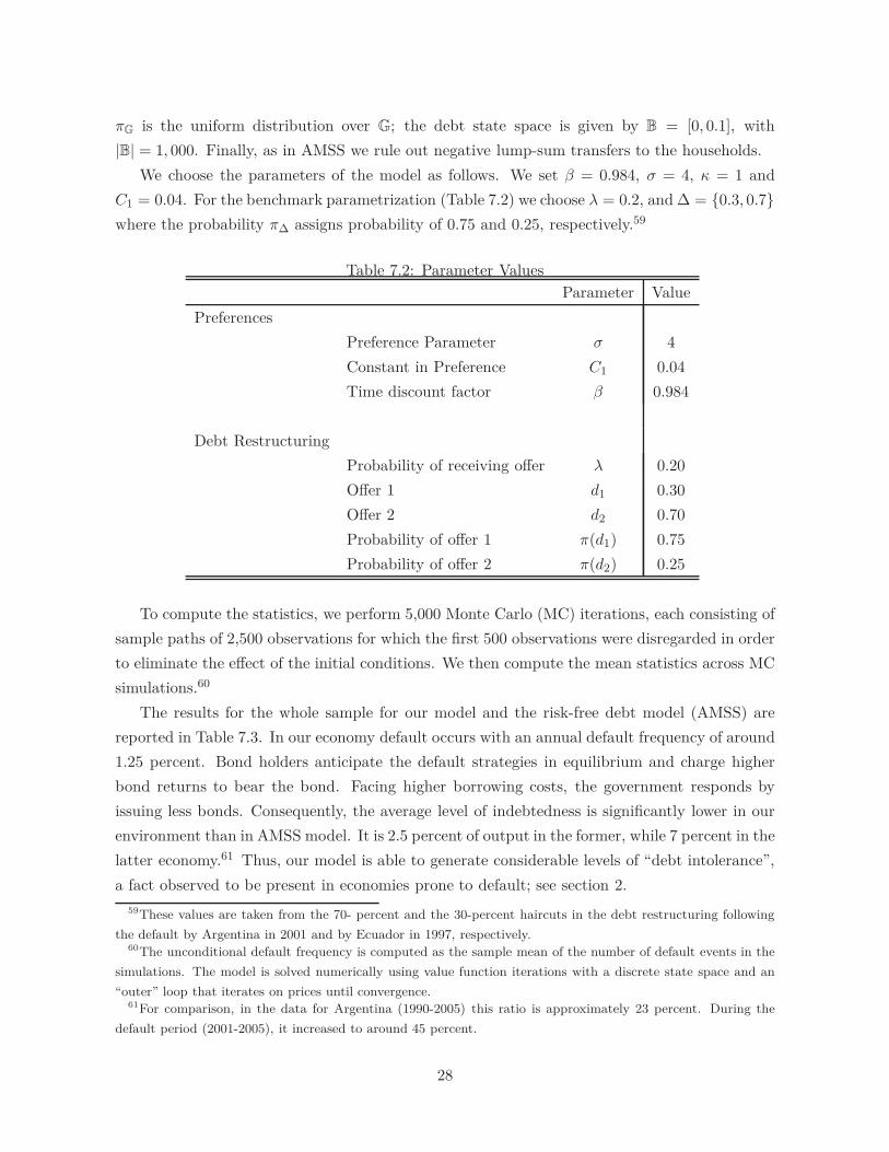
πG is the uniform distribution over G; the debt state space is given by B = [0, 0.1], with

|B| = 1, 000. Finally, as in AMSS we rule out negative lump-sum transfers to the households.

We choose the parameters of the model as follows. We set β = 0.984, σ = 4, κ = 1 and

C1 = 0.04. For the benchmark parametrization (Table 7.2) we choose λ = 0.2, and ∆ = 0.3, 0.7

where the probability π∆ assigns probability of 0.75 and 0.25, respectively.59

Table 7.2: Parameter Values

Parameter Value

Preferences

Preference Parameter σ 4

Constant in Preference C1 0.04

Time discount factor β 0.984

Debt Restructuring

Probability of receiving offer λ 0.20

Offer 1 d1 0.30

Offer 2 d2 0.70

Probability of offer 1 π(d1) 0.75

Probability of offer 2 π(d2) 0.25

To compute the statistics, we perform 5,000 Monte Carlo (MC) iterations, each consisting of

sample paths of 2,500 observations for which the first 500 observations were disregarded in order

to eliminate the effect of the initial conditions. We then compute the mean statistics across MC

simulations.60

The results for the whole sample for our model and the risk-free debt model (AMSS) are

reported in Table 7.3. In our economy default occurs with an annual default frequency of around

1.25 percent. Bond holders anticipate the default strategies in equilibrium and charge higher

bond returns to bear the bond. Facing higher borrowing costs, the government responds by

issuing less bonds. Consequently, the average level of indebtedness is significantly lower in our

environment than in AMSS model. It is 2.5 percent of output in the former, while 7 percent in the

latter economy.61 Thus, our model is able to generate considerable levels of “debt intolerance”,

a fact observed to be present in economies prone to default; see section 2.

59These values are taken from the 70- percent and the 30-percent haircuts in the debt restructuring following

the default by Argentina in 2001 and by Ecuador in 1997, respectively.60The unconditional default frequency is computed as the sample mean of the number of default events in the

simulations. The model is solved numerically using value function iterations with a discrete state space and an

“outer” loop that iterates on prices until convergence.61For comparison, in the data for Argentina (1990-2005) this ratio is approximately 23 percent. During the

default period (2001-2005), it increased to around 45 percent.

28

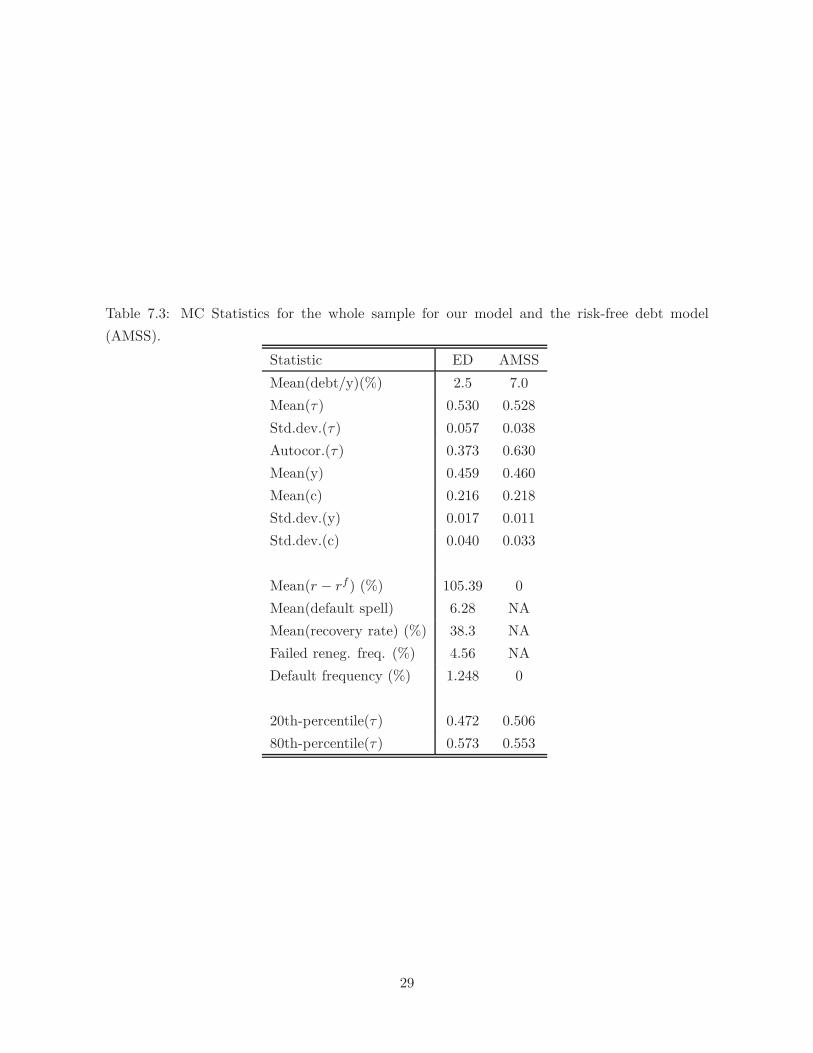
Table 7.3: MC Statistics for the whole sample for our model and the risk-free debt model

(AMSS).

Statistic ED AMSS

Mean(debt/y)(%) 2.5 7.0

Mean(τ) 0.530 0.528

Std.dev.(τ) 0.057 0.038

Autocor.(τ) 0.373 0.630

Mean(y) 0.459 0.460

Mean(c) 0.216 0.218

Std.dev.(y) 0.017 0.011

Std.dev.(c) 0.040 0.033

Mean(r − rf ) (%) 105.39 0

Mean(default spell) 6.28 NA

Mean(recovery rate) (%) 38.3 NA

Failed reneg. freq. (%) 4.56 NA

Default frequency (%) 1.248 0

20th-percentile(τ) 0.472 0.506

80th-percentile(τ) 0.573 0.553

29

Table 7.4: MC Statistics for the “financial autarky” sample and “financial access” sample.

Financial Access Financial Autarky

Statistic ED AMSS ED AMSS

Mean(debt/y)(%) 2.4 6.9 12.7 13.7

Mean(τ) 0.530 0.528 0.557 0.570

Std.dev.(τ) 0.056 0.038 0.093 0.053

Autocor.(τ) NA NA NA NA

Mean(y) 0.459 0.460 0.448 0.446

Mean(c) 0.217 0.218 0.201 0.200

std.dev.(y) 0.017 0.011 0.031 0.019

std.dev.(c) 0.040 0.033 0.054 0.039

Mean(r − rf ) (%) 3.40 0 6266.72 0

corr(y, r − rf ) -0.214 0 0 0

corr(τ , r − rf ) 0.181 0 0 0

20th-percentile(τ) 0.473 0.506 0.467 0.531

80th-percentile(τ) 0.572 0.552 0.663 0.608

The presence of endogenous borrowing limits, arising from the possibility of default, hinders

the government’s ability to smooth taxes. As a result, taxes are higher but particularly more

volatile: the standard deviation of tax rates is 50 percent higher in our model. Our model can

therefore replicate the corresponding empirical fact documented in section 2. Also, note that

the 20th-80th percentile interval for the tax distribution in the economy with defaultable bonds

contains its counterpart in the AMSS model, which reflects the fact that the latter distribution

is relatively more spread out. Not surprisingly, taxes are less persistent in our environment.62

The lower autocorrelation is attributed to two main factors. First, a lower persistence of taxes

in borrowing states due to the incidence of endogenous default, manifested in the law of motion

of the Lagrange multiplier of the implementability constraint; see subsection 6.2.63 Second,

the fact that if default occurs, the economy switches to autarky and the tax rate inherits the

stochastic properties of the government spending, which is assumed to be i.i.d. Finally, higher

and volatile taxes in our model lead to lower and more volatile labor supply.

Our model also generates a frequency of renegotiation failures of roughly 5 percent, an

average recovery rate of almost 40 percent, and a mean autarky spell of 6-7 periods.

62Since the “financial autarky” and “financial access” subsamples may contain nonconsecutive periods by con-

struction, the autocorrelation is not computed for them.63As discussed in subsection 6.2, the Lagrange multiplier in AMSS follows a martingale process.

30

While in table 7.3 we focus on the entire sample, in table 7.4 we show the results for two

subsamples: “financial autarky” and “financial access”. To construct these subsamples, we split

each MC simulation into the periods in which the ED economy is in autarky and those in which

it is not.

In this environment, the one-period gross risk-free 1+rf rate is equal to the reciprocal of the

households’ discount factor β. Bond spreads are computed as the differential between annualized

bond returns and the risk-free rate. The (one-period) gross return of the government bond is

given by 1/pt, both with borrowing and in financial autarky.64 As expected, our model is able

to generate higher spreads in financial autarky than in financial access. Bond spreads are on

average 3.4 percent with borrowing but jump to over 6, 000 percent in autarky. The particularly

high value of the spread in financial autarky reflects the fact that although the probability of

accepting an offer is around 95 percent, less than 40 percent of the defaulted debt is honored

and the probability of receiving an offer is only 2 percent. In the data we also observe such high

levels of bond yields during autarky: the average sovereign spreads measured by the EMBI+

index reached 5, 757 percent over 2002, the year after the default episode in Argentina, and

remained around 5, 485 percent between 2002 and 2004. Also, our model delivers countercyclical

bond spreads, a feature well-documented in the data for emerging economies.65 As indicated

by the positive correlation between tax rates and spreads, taxes tend to be higher precisely

when borrowing is more expensive. Labor supply is optimally lower in those states leading to a

negative co-movement between bond returns and output.

During financial autarky, the average debt-to-output ratio is actually the defaulted debt-to-

output ratio and is around 13 percent. The fact that it is roughly five times larger than in

financial access provides additional evidence of endogenous borrowing limits being “active” for

high debt levels, this is consistent with the stylized facts presented in section 2.

The findings for taxes in financial access and financial autarky echo the results in Table 7.3.

When there is borrowing, taxes are relatively more volatile in the economy with the defaultable

bond due to the endogenous credit limits. Furthermore, when our economy is in financial

autarky, the government is precluded from issuing debt, rendering taxes more volatile that

in financial access. The 20th-80th percentile intervals for taxes are consistent with the same

patterns.

64This calculation of the bond return during autarky is reminiscent to the methodology applied by J.P. Morgan

to obtain sovereign bond yields and spreads for the construction of the EMBI+ index. While a country is in default

before any debt settlement is reached, bond yields and spreads are calculated assuming future cash flows stay

the same as dictated in the original instrument structure. In this situation, future cash flows are not determined

based on any expected haircuts until after a restructuring event officially takes place. For more details, see J. P.

Morgan (2004).65For both output and tax rates, the correlations with bond spreads are zero in autarky since government

spending is i.i.d. —hence prices only depend on the debt level, as shown in expressions 6.21 and 6.22— and bond

holdings remain unchanged until the debt is restructured.

31

Figure 7.3: Standard deviation of tax rates and mean bond spreads in financial access for low

debt (blue) and high debt (red).

Both the average output and consumption are similar in both economies, although in both

cases these quantities are higher in the financial access subsample. Financial autarky is charac-

terized by on average higher indebtedness levels and also slightly higher government expenditure

(not reported), that is, higher expenditure overall. Given that the primary surplus function z

is decreasing in n, it follows that output (and consumption) are lower during financial autarky.

This fact shows that our model is able to endogenously generate a drop in output (and con-

sumption) during this period, even though no ad-hoc output loss is assumed in this calibration.

In addition, in both economies output and consumption are more volatile in the financial

autarky subsample. The fact that the primary surplus function is also concave implies a higher

sensitivity of these variables to changes in government spending and thus higher volatility during

financial autarky. Finally, both output and consumption are more volatile in our economy than

in AMSS, portraying the differences in the dynamics of their taxes.

Behavior of Taxes. As mentioned in section 2, our dataset suggests that default risk and

tax volatility are positively correlated and that both are higher for high levels of debt-to-output

ratio. Figure 7.3 shows that our model is able to generate this pattern. The blue (red) dots

show the standard deviation of taxes and spreads for low (high) levels of debt, respectively.

Each dot corresponds to the financial access subsample in a MC simulation. For low (high) debt

we consider debt-to-output ratios below (over) the median of its distribution. For both cases

32

0.4 0.45 0.5 0.55 0.6 0.650

20

40

0.4 0.45 0.5 0.55 0.6 0.650

20

40

0.4 0.45 0.5 0.55 0.6 0.650

50

100

0.4 0.45 0.5 0.55 0.6 0.650

50

100

0.4 0.45 0.5 0.55 0.6 0.650

25

50

Figure 7.4: Histograms of tax rates in financial access for our model (solid red) and AMSS

(dotted blue) conditioned on current g realization, from lowest value (top panel) to highest

value (bottom panel).

33

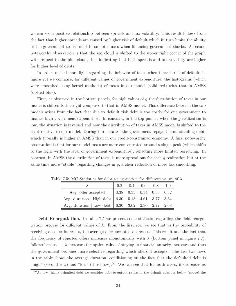
we can see a positive relationship between spreads and tax volatility. This result follows from

the fact that higher spreads are caused by higher risk of default which in turn limits the ability

of the government to use debt to smooth taxes when financing government shocks. A second

noteworthy observation is that the red cloud is shifted to the upper right corner of the graph

with respect to the blue cloud, thus indicating that both spreads and tax volatility are higher

for higher level of debts.

In order to shed more light regarding the behavior of taxes when there is risk of default, in

figure 7.4 we compare, for different values of government expenditure, the histograms (which

were smoothed using kernel methods) of taxes in our model (solid red) with that in AMSS

(dotted blue).

First, as observed in the bottom panels, for high values of g the distribution of taxes in our

model is shifted to the right compared to that in AMSS model. This difference between the two

models arises from the fact that due to default risk debt is too costly for our government to

finance high government expenditure. In contrast, in the top panels, when the g realization is

low, the situation is reversed and now the distribution of taxes in AMSS model is shifted to the

right relative to our model. During those states, the government repays the outstanding debt,

which typically is higher in AMSS than in our credit-constrained economy. A final noteworthy

observation is that for our model taxes are more concentrated around a single peak (which shifts

to the right with the level of government expenditure), reflecting more limited borrowing. In

contrast, in AMSS the distribution of taxes is more spread-out for each g realization but at the

same time more “stable” regarding changes in g, a clear reflection of more tax smoothing.

Table 7.5: MC Statistics for debt renegotiation for different values of λ.

λ 0.2 0.4 0.6 0.8 1.0

Avg. offer accepted 0.38 0.35 0.34 0.33 0.32

Avg. duration | High debt 6.30 5.18 4.61 3.77 3.34

Avg. duration | Low debt 6.30 3.62 2.90 2.77 2.68

Debt Renegotiation. In table 7.5 we present some statistics regarding the debt renego-

tiation process for different values of λ. From the first row we see that as the probability of

receiving an offer increases, the average offer accepted decreases. This result and the fact that

the frequency of rejected offers increases monotonically with λ (bottom panel in figure 7.7),

follows because as λ increases the option value of staying in financial autarky increases and thus

the government becomes more selective regarding which offers it accepts. The last two rows

in the table shows the average duration, conditioning on the fact that the defaulted debt is

“high” (second row) and “low” (third row).66 We can see that for both cases, it decreases as

66As low (high) defaulted debt we consider debt-to-output ratios in the default episodes below (above) the

34

the probability of receiving an offer increases, but more importantly it shows that for “high”

levels of debt we have, on average, longer financial autarky spells; in fact, the difference can

be as large as 50 percent higher for intermediate values of λ. This result coincides with the

implications of proposition 6.1. Moreover, as we see from the table, differences in the duration

can be non-negligible.

Impulse responses. Figure 7.5 plots the impulse response for debt and taxes for our model

and AMSS. The path of government expenditure is plotted in the first panel: the government

expenditure is low and equal to 0.224 except for t = 2, ..., 6 where it is high and equal to 0.26.

We consider two values of initial debt, one “low” (B0 = 0) and one “high” (B0 = 0.05). To

finance high government expenditure during the first periods, the government makes use of both

instruments: bond issuance and taxes. While in both economies the government accumulates

debt in those periods, in our model it does so to a lesser extent due to the presence of endogenous

borrowing limits. From t = 7 onwards, when government expenditure becomes low, the level of

debt decreases, eventually reaching zero. Taxes behave analogously.

In our economy taxes are higher than AMSS during the periods of high government expen-

diture since borrowing is more limited, but they decrease more rapidly when the realization of

government expenditure becomes lower (see the third panel). Overall, not surprisingly, one can

see a smoother behavior for taxes in AMSS than in our economy. The last panel plots the behav-

ior of the Lagrange multiplier νt studied in subsection 6.2. The fact that ours is above the one

of AMSS for periods of high government expenditure reflects the “mark-up” effect mentioned in

subsection 6.2. Also note that the Lagrange multiplier increases during these periods, reflecting

the fact that the marginal cost of debt is increasing in the level of debt. From t = 6 onwards, as

debt decreases, the Lagrange multiplier in our model falls and eventually becomes lower than

the one of AMSS. This last feature stems from the facts that the accumulated debt is relatively

lower in our model and that, as the level of debt decreases, the “mark-up” effects vanish.

Welfare Analysis. As a measure of welfare we use the compensation in terms of initial con-

sumption that would make the household indifferent between our economy and AMSS. Formally,

this compensation denoted by W is computed as

W ≡

∫V AMSS(g, B)µAMSS(dg, dB) −

∫V ∗

φ (g, B)µ(dg, dB, dφ)∫

(n∗φ(g, B) − g)µ(dg, dB, dφ)

where µAMSS and µ are the ergodic distributions generated by the AMSS and our model re-

spectively and V AMSS is the value function corresponding to the AMSS economy. That is, W

measures the increase in initial consumption that would make the household indifferent between

our economy and AMSS, under the ergodic distribution.67

unconditional median.67The ergodic distribution is constructed by collecting the last observation from each of the 5,000 MC simulated

paths.

35

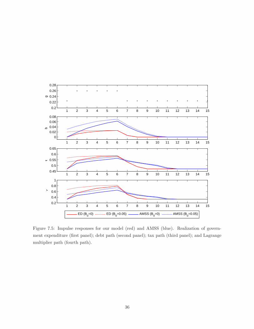
1 2 3 4 5 6 7 8 9 10 11 12 13 14 150.2

0.22

0.24

0.26

0.28

g

1 2 3 4 5 6 7 8 9 10 11 12 13 14 15

0

0.02

0.04

0.06

0.08

b

1 2 3 4 5 6 7 8 9 10 11 12 13 14 150.45

0.5

0.55

0.6

0.65

1 2 3 4 5 6 7 8 9 10 11 12 13 14 150.2

0.4

0.6

0.8

1

ED (B0=0) ED (B

0=0.05) AMSS (B

0=0) AMSS (B

0=0.05)

Figure 7.5: Impulse responses for our model (red) and AMSS (blue). Realization of govern-

ment expenditure (first panel); debt path (second panel); tax path (third panel); and Lagrange

multiplier path (fourth path).

36

0.1 0.2 0.3 0.4 0.5 0.6 0.7 0.8 0.9 10

0.1

0.2

0.3

0.4

0.5

0.6

0.7

compensation W fraction of time in autarky

Figure 7.6: Consumption compensation W (solid blue) and fraction of time in autarky under

ergodic distribution (dashed green) for different values of arrival probability of offers λ.

0.1 0.2 0.3 0.4 0.5 0.6 0.7 0.8 0.9 10

5

10

15

20

Ave

rage

num

ber

of p

erio

ds in

aut

arky

0.1 0.2 0.3 0.4 0.5 0.6 0.7 0.8 0.9 10

0.1

0.2

0.3

0.4

0.5

Fre

quen

cy o

f fai

led

rene

gotia

tions

Figure 7.7: Average number of periods in autarky (top panel) and frequency of rejected offers

(bottom panel) for different values of arrival probability of offers λ.

37

Figure 7.6 plots this measure for different values of the arrival probability of offers λ with

our, otherwise, benchmark parametrization. As we can see, for low values of λ the compensa-

tion is almost zero, which is consistent with the fact that in these cases autarky is very costly

pushing down the default frequency and thereby implying that our economy and AMSS are

very similar. As λ increases, default occurs more often and welfare decreases in our economy

relative to AMSS. In particular, for λ = 0.7 the compensation is as high as 63.64 percent of the

initial consumption. Welfare, however, does not decrease monotonically with λ. In fact, for λ

ranging from 0.7 to 1, welfare increases in our economy. A key effect for understanding this

non-monotonicity is the behavior of the government during financial autarky. The average time

the economy spends in financial autarky decreases monotonically, especially for low values of λ

(top panel in figure 7.7), and perhaps more importantly the frequency of rejected offers increases

monotonically with λ (bottom panel in figure 7.7) as well. These facts imply that, for high values

of λ, the government is frequently confronted with the option to reject a repayment offer and

stay in financial autarky, whereas for low values of λ, this option is presented more infrequently.

Thus, roughly speaking, for high values of λ, the time the economy spends in financial autarky

is not only low but is driven by choice, whereas for low values of λ it is not. This last observation

explains the non-monotonic behavior of welfare with respect to λ and also presents a nuanced

view for evaluating how costly renegotiations periods are. In particular, longer spells in financial

autarky does not necessarily imply lower welfare.

Robustness check: Persistent process for government expenditure. We explore the

quantitative implications of our model under the assumption of persistence on the stochastic

process for government expenditure. To do so, we use a 3-state Markov chain for gt given by

πG =

0.5 0.5 0

0.1 0.8 0.1

0 0.5 0.5

.

We interpret this state space as a “expansionary”, “normal” and “contractionary” govern-

ment expenditures. We assume that normal times are more persistent than the other two states,

and for simplicity we treat these two states symmetrically. Besides the stochastic process gov-

ernment expenditure, the parametrization is the same as in our benchmark calibration, except

that the probability of offer arrival λ is set to 0.18, and the offer space is ∆ = 0, 0.35, 0.7

with a probability distribution over it given by π∆ = 0.3, 0.4, 0.3. For comparison, we also

present the case with i.i.d. government expenditure, drawn from the invariant distribution of the

Markov chain. By using the invariant distribution, we are able to isolate the effect of changing

the dependence structure of government expenditure, from other changes in the distribution

such as changes in mean or variance.68

68Formally, since in the i.i.d. case we use the (unique) invariant distribution, as the number of observation goes

38

Table 7.6 reports the MC statistics for our economy and AMSS. When government expen-

diture is more persistent, default tends to occur more often. The annual default frequency is

around 3.8 percent with persistent g while it only reaches 0.3 percent in the i.i.d. case. The

government generally decides to default after a sufficiently long sequence of high government

expenditure after increasing substantially its debt level; such sequences are more likely to occur

with persistent g than in the i.i.d. case.

For AMSS the autocorrelation of taxes is roughly the same for both cases, the persistent one

and the i.i.d. one. This is consistent with the intuition derived in Aiyagari et al. (2002) (see

also section 6.2) which implies that optimal taxes are highly persistent, even if the government

expenditure is i.i.d. As mentioned above, taxes are less persistent in our environment, because

of the incidence of endogenous default (see subsection 6.2) and because of the fact that if default

occurs, the economy switches to autarky and the tax rate inherits the stochastic properties of

the government spending. An interesting implication of this result is that our model predicts a

tighter (and positive) link between autocorrelation of taxes and autocorrelation of government

expenditures than AMSS.

As noted before, the debt-to-output ratio is lower in ED than in AMSS due to the endogenous

borrowing limits. In both cases, ED and AMSS, there is less borrowing in the persistence case.

The intuition of this last fact is straightforward. In the persistent case, ”expansionary” govern-

ment expenditures are expected to last longer than in the i.i.d. case, thus creating incentives to

increase more taxes and issue less debt (than in the i.i.d.) case.69 For the ”normal” government

expenditure case, the conditional transition matrix yields probabilities for tomorrow’s state that

are very similar to those in the i.i.d. distribution.

The previous forces also explain why taxes are more volatile in the persistent case (for both

ED and AMSS). As in the benchmark specification, we observe higher tax variability in our

model than in AMSS.

Robustness check: Aversion to Consumption Risk. In previous calibrations we as-

sumed that households were consumption-risk neutral by endowing them with quasi-linear pref-

erences. In what follows we relax this assumption by considering a balanced growth prefer-

ence specification, as in Aiyagari et al. (2002) and Farhi (2010). More specifically, we assume

u(c, 1 − n) = log c + C1(1−n)1−σ

1−σ, with C1 = 0.02 and σ = 3. For computational purposes, in

this new calibration, the government spending shock can only take two values: gH (”expansion-

ary”) and gL (”normal”), with gH > gL. It is assumed to be i.i.d. with transition probability

πG(gL) = 0.9. There is only one debt renegotiation offer d = 0.7 with arrival probability λ = 0.15

and no ad-hoc output cost for default. In this setup, with consumption-risk aversion, the low

to infinity, any sample moment (mean, variance, etc) of the government shock for the i.i.d. case converges to the

one for the persistent case.69Similarly, the ”contractionary” phase is expected to last longer as well, thus creating incentives to lower taxes,

relative to the i.i.d. cases.

39

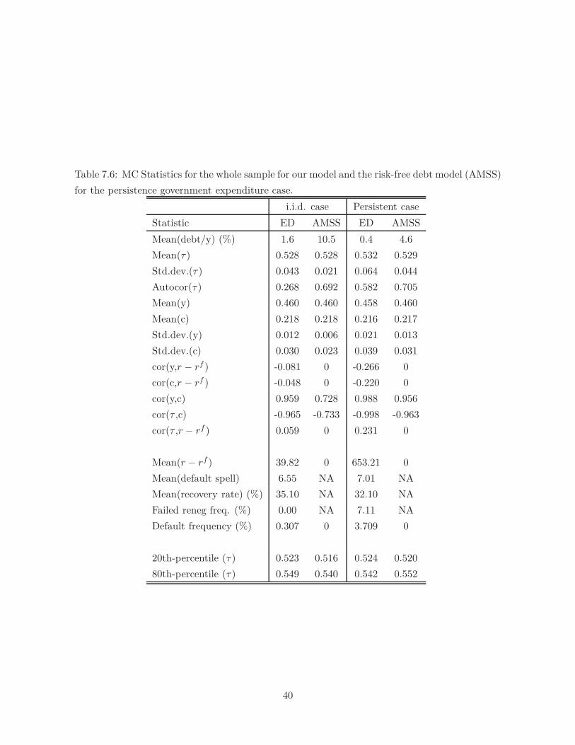
Table 7.6: MC Statistics for the whole sample for our model and the risk-free debt model (AMSS)

for the persistence government expenditure case.

i.i.d. case Persistent case

Statistic ED AMSS ED AMSS

Mean(debt/y) (%) 1.6 10.5 0.4 4.6

Mean(τ) 0.528 0.528 0.532 0.529

Std.dev.(τ) 0.043 0.021 0.064 0.044

Autocor(τ) 0.268 0.692 0.582 0.705

Mean(y) 0.460 0.460 0.458 0.460

Mean(c) 0.218 0.218 0.216 0.217

Std.dev.(y) 0.012 0.006 0.021 0.013

Std.dev.(c) 0.030 0.023 0.039 0.031

cor(y,r − rf ) -0.081 0 -0.266 0

cor(c,r − rf ) -0.048 0 -0.220 0

cor(y,c) 0.959 0.728 0.988 0.956

cor(τ ,c) -0.965 -0.733 -0.998 -0.963

cor(τ ,r − rf ) 0.059 0 0.231 0

Mean(r − rf ) 39.82 0 653.21 0

Mean(default spell) 6.55 NA 7.01 NA

Mean(recovery rate) (%) 35.10 NA 32.10 NA

Failed reneg freq. (%) 0.00 NA 7.11 NA

Default frequency (%) 0.307 0 3.709 0

20th-percentile (τ) 0.523 0.516 0.524 0.520

80th-percentile (τ) 0.549 0.540 0.542 0.552

40

probability of occurrence of gH together with the relatively low value of λ are sufficient to deter

the government from defaulting too often. The time discount factor is set to 0.983.

Table 7.7 reports the MC statistics for our model with default and the risk-free debt model

(AMSS). The main features observed in previous calibrations continue to hold for this case

with consumption-risk aversion, namely, taxes are more volatile and less persistent and debt is

lower in the presence of default risk. In particular, taxes are approximately 25 percent more

volatile in our economy than in the AMSS one. Also, in our model, default occurs with an

annual frequency of over 3.64 percent, which is priced in by the household and, consequently,

we observe approximately 45 percent less borrowing in our economy.

Under our assumption on preferences, there is a strong negative co-movement between con-

sumption and both labor supply and taxes in the two economies. As the tax rate increases,

consumption drops and the household supplies more labor due to the non-zero ”wealth” effect.

Moreover, as taxes are usually higher in states with default risk, labor supply tends to also

be high in those states, which explains the weakly pro-cyclical interest rates observed in this

calibration.70

Finally, a novel feature of defaulting in this environment with commitment to fiscal policies

is that it allows for a resetting of taxes. While in our economy eventually after every default

episode the fiscal authority has the chance to review and re-optimize its tax rates, in the AMSS

model this is not the case, as the government is bound by previous marginal utility promises.

Therefore, in the latter environment, taxes may stay high and persistent in states with high

indebtedness as the economy hovers around the ad hoc borrowing limits.

Defaulting in our environment acts as “loose commitment device” in the spirit of Debortoli

and Nunes (2010). We believe it captures, up to some extent, the fact that after several default

episodes, we observe changes in the composition of the ruling political authority and in its

underlying policies; e.g. Argentina (2001) and Greece (2011). It could be interesting to see how

our results change when allow for alternative ways in which the fiscal authority could choose

policies after debt restructuring periods; we leave this as future research.

8 Conclusion

In this paper we study a government problem in a closed economy that consists of choosing

distortionary taxes with only non-state-contingent government debt, but allowing for partial

payments of defaulted debt.

First, we provide an explanation for the lower debt-to-output ratios and more volatile tax

policies observed in emerging economies, vis-a-vis industrialized economies. This stems from the

70This implication of the model is clearly not in line with the data for emerging economies. More realistic

results along this dimension call for a utility function different from the balanced growth preference specification

used by Aiyagari et al. (2002) and Farhi (2010).

41

Table 7.7: MC Statistics for the whole sample for our model and the risk-free debt model

(AMSS).

Statistic ED AMSS

Mean(debt/y)(%) 0.49 0.77

Mean(τ) 0.3047 0.3050

Std.dev.(τ) 0.0155 0.0125

Autocor.(τ) 0.2652 0.5576

Mean(y) 0.7530 0.7530

Mean(c) 0.5237 0.5237

Std.dev.(y) 0.0009 0.00154

Std.dev.(c) 0.0152 0.0147

cor(y,r − rf ) 0.0607 0

cor(c,r − rf ) -0.2476 0

cor(y,c) -0.7687 -0.7876

cor(τ ,c) -0.9525 -0.7778

cor(τ ,r − rf ) 0.2931 0

Mean(r − rf ) (%) 35.992 0

Mean(rf ) (%) 7.731 7.643

Mean(default spell) 7.67 NA

Mean(recovery rate) (%) 0.70 NA

Failed reneg. freq. (%) 0.00 NA

Default frequency (%) 3.638 0

20th-percentile(τ) 0.2975 0.2975

80th-percentile(τ) 0.3070 0.3182

42

fact that the holders of government debt forecast the possibility of default, imposing endogenous

debt limits. These limits restrict the ability of the government to smooth shocks using debt,

resulting in higher tax variability.

Second, we propose a device to price the debt during temporary financial autarky. Our

results show that the spread during the default period is higher than for the rest of the sample;

this characteristic is consistent with data for defaulters—e.g., Argentina, Ecuador and Russia.

Third, and last, the numerical simulations suggest that increasing the probability of receiving

offers for exiting autarky decreases welfare when this probability is low/medium to begin with,

but increases it when the probability is high.

Although this model does a good job of explaining qualitatively several empirical regularities,

it could be enriched in several dimensions so as to better fit the data of particular economies.

More precisely, we think a promising line of future research could be to extend the production

side of this economy to allow for physical capital accumulation and productivity shocks. Our

model also provides a novel device that allow us to study asset prices of government debt

both during periods of financial access and autarky; further research could fully explore the

pricing implications of this device for general sovereign debt held by uncertainty or risk averse

creditors.71

References

Abreu, D., Pearce, D., and Stacchetti, E. (1990). Toward a theory of discounted repeated games

with imperfect monitoring. Econometrica, 58:1041–1063.

Aguiar, M., Amador, M., and Gopinath, G. (2009). Investment cycles and sovereign debt

overhang. Review of Economic Studies, 76(1):1–31.

Aguiar, M. and Gopinath, G. (2006). Defaultable debt, interest rates and the current account.

Journal of International Economics, 69(1):64–83.

Aiyagari, R., Marcet, A., Sargent, T., and Seppala, J. (2002). Optimal taxation without state

contingent debt. Journal of Political Economy, 110:1220–1254.

Arellano, C. (2008). Default risk and income fluctuations in emerging economies. American

Economic Review, 98(3):690–713.

Bai, Y. and Zhang, J. (2012). Duration of sovereign debt renegotiation. Journal of International

Economics, 86:252–268.

Benjamin, D. and Wright, M. (2009). Recovery before redemption: A theory of delays in

sovereign debt renegotiations. Mimeo, Dept of Economics, UCLA.

71See Aguiar and Gopinath (2006) and Mendoza and Yue (2012), and Pouzo and Presno (2013).

43

Broner, F., Martin, A., and Ventura, J. (2010). Sovereign risk and secondary markets. American

Economic Review, 100(4):1523–1555.

Chang, R. (1998). Credible monetary policy in a infinite horizon model: Recursive approaches.

Journal of Economic Theory, 81:431–461.

Chatterjee, S. and Eyingungor, B. (2012). Maturity, indebtedness, and default risk. American

Economic Review, 102(6):2674–99.

Cruces, J. and Trebesch, C. (2013). Sovereign defaults: The price of haircuts. American Eco-

nomic Journal: Macroeconomics, 5(3):85–117.

Cuadra, G., Sanchez, J. M., and Sapriza, H. (2010). Fiscal policy and default risk in emerging

markets. Review of Economic Dynamics, 13(2):919–933.

Debortoli, D. and Nunes, R. (2010). Fiscal policy under loose commitment. Journal of Economic

Theory, 145(3).

Doda, B. (2007). Optimal fiscal policy with sovereign default. Mimeo, Dept of Economics, Univ.

of Toronto.

Eaton, J. and Gersovitz, M. (1981). Debt with potential repudiation: Theoretical and empirical

analysis. Review of Economic Studies, 48(2):289–309.

Farhi, E. (2010). Capital taxation and ownership when markets are incomplete. Journal of

Political Economy, 118:908–948.

Hopeynhan, H. and Werning, I. (2009). Equilibrium default. Mimeo UCLA.

Kaminsky, G., Reinhart, C., and Vegh, C. (2004). When it rains, it pours: Procyclical cap-

ital flows and macroeconomic policies. NBER Working Papers 10780, National Bureau of

Economic Research, Inc.

Koenker, R. (2005). Quantile Regression. Econometric Society Monograph Series. Cambridge

University Press.

Kydland, F. and Prescott, E. (1980). Dynamic optimal taxation, rational expectations and

optimal control. Journal of Economic Dynamics and Control, 2:79–91.

Lucas, R. and Stokey, N. L. (1983). Optimal fiscal and monetary policy in an economy without

capital. Journal of Monetary Economics, 12(1):55–93.

Magill, M. and Quinzii, M. (1994). Infinite horizon incomplete markets. Econometrica, 62:853–

880.

44

Mendoza, E. and Yue, V. (2012). A general equilibrium model of sovereign default and business

cycles. Quaterly Journal of Economics, 127(2):889–946.

Morgan, J. P. (2004). Emerging markets bond index plus (embi+), rules and methodology.

Emerging Markets Research.

Panizza, U. (2008). Domestic and external public debt in developing countries. Technical Report

188, United Nations conference on trade and development.

Pitchford, R. and Wright, M. (2008). Restructuring the sovereign debt restructuring mechanism.

Mimeo, dept. of Economics, Univ. of Sidney and UCLA.

Pouzo, D. and Presno, I. (2013). Sovereign default risk and uncertainty premia. Mimeo, UC

Berkeley.

Reinhart, C. and Rogoff, K. (2008). The forgotten history of domestic debt. Working Paper

13946, National Bureau of Economic Research.

Reinhart, C., Rogoff, K., and Savastano, M. (2003). Debt intolerance. Working Paper 9908,

National Bureau of Economic Research.

Stokey, N., Lucas, R., and Prescott, E. (1989). Recursive Methods in Economic Dynamics.

Harvard University Press.

Sturzenegger, F. and Zettelmeyer, J. (2006). Debt Defaults and Lessons from a Decade of Crises.

The MIT press.

Yue, V. (2010). Sovereign default and debt renegotiation. Journal of International Economics,

80(2):176–187.

45

A Notation and Stochastic Structure of the Model

Throughout the appendix for a generic mapping f from a set S to T , we use s 7→ f(s) or f : S → T

to denote it. For the case that a mapping depends on many variables, the notation s1 7→ f(s1, s2)

is used to denote the function f only as a function of s1, keeping s2 fixed. Also, for a generic set

A, |A| denotes the cardinality of A.

B Optimization Problem for the Households

The Lagrangian associated to the household’s problem is given by

L(ct, nt, bt+1, νt, µt, ψt∞t=0) ≡

∞∑

t=0

βtEΠ(·|ω0)

[u(ct(ω

t), 1 − nt(ωt)) − νt(ω

t)ct(ωt) − (1 − τt(ω

t))κt(ωt)nt(ω

t) + pt(ωt)bt+1(ωt) − t(ω

t)bt(ωt−1)

+ Ψt(ωt)ct(ω

t) + ψ1t(bt+1(ωt) − b) + ψ2t(b− bt+1(ωt))],

where νt and Ψt are the Lagrange multipliers associated to the budge constraint and to the

restrictions that non-negative bound on consumption, and ψit i = 1, 2 are the Lagrange multipliers

associated to the debt limits.

Assuming interiority of the solutions, the first order conditions (FONC) are given by:

ct(ωt) : uc(ct(ω

t), 1 − nt(ωt)) − νt(ω

t) = 0

nt(ωt) : − ul(ct(ω

t), 1 − nt(ωt)) + νt(ω

t)(1 − τt(ωt))κt(ω

t) = 0

bt+1(ωt) : pt(ωt)νt(ω

t) − EΠ(·|ωt)[βνt+1(ωt+1)t+1(ωt+1)] = 0.

Then, using uj(ωt) for uj(ct(ω), 1 − nt(ω)) with j ∈ c, l, it follows

ul(ωt)

uc(ωt)= (1 − τt(ω

t))κt(ωt), (B.24)

and

pt(ωt) = EΠ(·|ωt)

[βuc(ω

t+1)

uc(ωt)t+1(ωt+1)

]. (B.25)

From the definition of , equation B.25 implies, for φt = 1 ,

pt(ωt) = EΠ(·|ωt)

[βuc(ω

t+1)

uc(ωt)(1 − dt+1(ω))

]+ EΠ(·|ωt)

[βuc(ω

t+1)

uc(ωt)dt+1(ωt+1)qt+1(ωt+1)

].

For φt = 0, (where in this case recall that pt = qt)

pt(ωt) = λEΠ(·|ωt)

[βuc(ω

t+1)

uc(ωt)at+1(ωt+1)δt+1

]

+ EΠ(·|ωt)

[βuc(ω

t+1)

uc(ωt)1 − λ+ λ(1 − at+1(ωt+1))qt+1(ω

t+1)

].

46

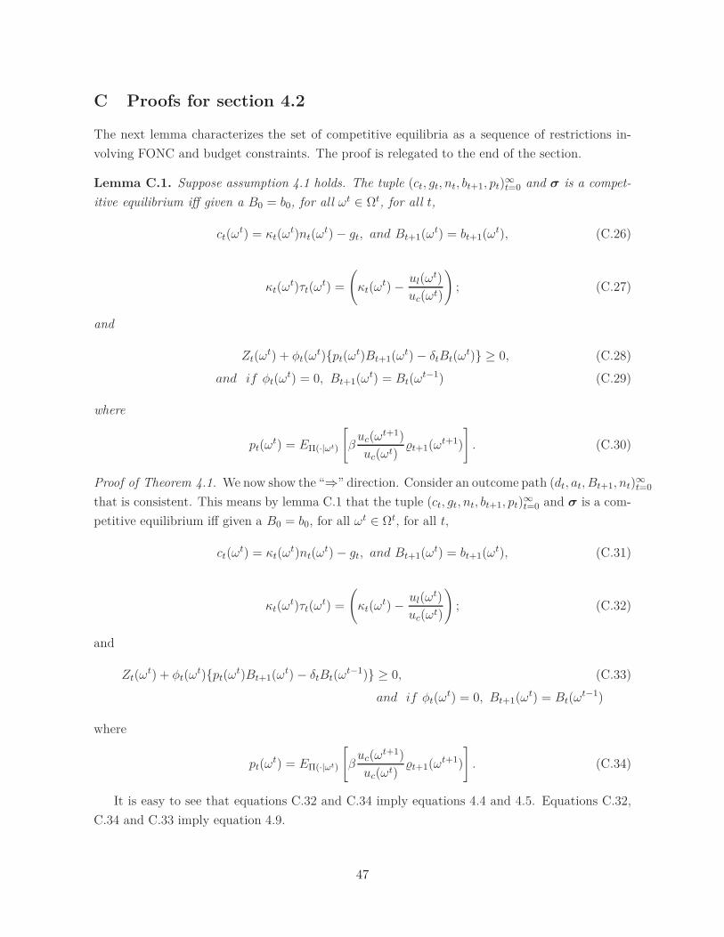
C Proofs for section 4.2

The next lemma characterizes the set of competitive equilibria as a sequence of restrictions in-

volving FONC and budget constraints. The proof is relegated to the end of the section.

Lemma C.1. Suppose assumption 4.1 holds. The tuple (ct, gt, nt, bt+1, pt)∞t=0 and σ is a compet-

itive equilibrium iff given a B0 = b0, for all ωt ∈ Ωt, for all t,

ct(ωt) = κt(ω

t)nt(ωt) − gt, and Bt+1(ωt) = bt+1(ωt), (C.26)

κt(ωt)τt(ω

t) =

(κt(ω

t) −ul(ω

t)

uc(ωt)

); (C.27)

and

Zt(ωt) + φt(ω

t)pt(ωt)Bt+1(ωt) − δtBt(ω

t) ≥ 0, (C.28)

and if φt(ωt) = 0, Bt+1(ωt) = Bt(ω

t−1) (C.29)

where

pt(ωt) = EΠ(·|ωt)

[βuc(ω

t+1)

uc(ωt)t+1(ωt+1)

]. (C.30)

Proof of Theorem 4.1. We now show the “⇒” direction. Consider an outcome path (dt, at, Bt+1, nt)∞t=0

that is consistent. This means by lemma C.1 that the tuple (ct, gt, nt, bt+1, pt)∞t=0 and σ is a com-

petitive equilibrium iff given a B0 = b0, for all ωt ∈ Ωt, for all t,

ct(ωt) = κt(ω

t)nt(ωt) − gt, and Bt+1(ωt) = bt+1(ωt), (C.31)

κt(ωt)τt(ω

t) =

(κt(ω

t) −ul(ω

t)

uc(ωt)

); (C.32)

and

Zt(ωt) + φt(ω

t)pt(ωt)Bt+1(ωt) − δtBt(ω

t−1) ≥ 0, (C.33)

and if φt(ωt) = 0, Bt+1(ωt) = Bt(ω

t−1)

where

pt(ωt) = EΠ(·|ωt)

[βuc(ω

t+1)

uc(ωt)t+1(ωt+1)

]. (C.34)

It is easy to see that equations C.32 and C.34 imply equations 4.4 and 4.5. Equations C.32,

C.34 and C.33 imply equation 4.9.

47

We now show the “⇐” direction. Suppose now that the outcome path satisfies that for all

ωt ∈ Ωt, the following equations holds: 4.4, 4.5, 4.9 and

ct(ωt) = κt(ω

t)nt(ωt) − gt. (C.35)

By using Bt+1(ωt) = bt+1(ωt), equations 4.4, 4.5 and the feasibility condition, we can enlarge

the outcome path by (ct, pt, bt+1, τt, gt)∞t=0. Clearly, restrictions C.31, C.32 and C.34 hold. By

replacing equations 4.4 and 4.5 on 4.9, it is easy to see that equation C.33 holds too.

C.1 Proofs of supplementary lemmas

For the proof of Lemma C.1 we need the following lemma (the proof is relegated to the end of

the section).

Lemma C.2. Suppose assumption 4.1 holds. Then first order conditions 4.4 and 4.5 are also

sufficient.

Proof of Lemma C.1. Take σ and (ct, gt, nt, bt+1)∞t=0, and a price schedule (pt)t that satisfy the

equations. It is easy to see that feasibility and market clearing holds (conditions 3 and 4). Also,

by lemma C.2 optimality of the households is also satisfied.

To check attainability of the government policy (condition 2). Observe that by equations C.26

- C.28 imply for all ωt ∈ Ωt,

gt + φt(ωt)δtBt(ω

t−1) − φt(ωt)pt(ω

t)Bt+1(ωt) ≤ κt(ωt)τt(ω

t)nt(ωt).

Finally, we check optimality of the households. We first check that the sequences satisfy the

budget constraint. Observe that by equations C.26 - C.28

−ct(ωt) + κt(ω

t)nt(ωt) + φt(ω

t)δtBt(ωt−1) − pt(ω

t)Bt+1(ωt) ≤ κt(ωt)τt(ω

t)nt(ωt).

If φt(ωt) = 1, then equation C.28 implies that bt+1(ωt) = Bt+1(ωt) for all t (and for b0 we

assume it is equal to B0) and thus

− ct(ωt) + κt(ω

t)nt(ωt) + δtbt(ω

t−1) − pt(ωt)bt+1(ωt) ≤ κt(ω

t)τt(ωt)nt(ω

t).

This coincides with the budget constraint of the household.

If dt(ωt) = 1, but at(ω

t) = 0, then equations C.26 and C.28 imply that bt(ωt−1) = bt+1(ωt) = 0

for all t, so

−ct(ωt) + κt(ω

t)nt(ωt) = κt(ω

t)τt(ωt)nt(ω

t).

This coincides with the budget constraint of the household.

Take σ and (ct, gt, nt, bt+1, pt)∞t=0 being a competitive equilibrium. Then it is easy to see that

it satisfies the equations.

48

Proof of Lemma C.2. Under assumption 4.1 the objective function of the household optimization

problem is strictly concave. The budget constraints and debt constraint form a convex set of

constraints. Thus, if the transversality condition holds, the FONC are sufficient; this follows from

a simple adaptation of the results in Stokey et al. (1989) Ch. 4.5.

In order to verify the transversality condition, it suffices to show that for any ζt(ωt) such that

bt(ωt) + ζt(ω

t) ∈ B,

limT →∞

βTEΠ[uc(κT (ωT )nT (ωT ) − gT , 1 − nT (ωT ))T (ωT )ζT (ωT )] = 0.

Since, by assumption, debt is constrained, this condition follows from Magill and Quinzii

(1994) Theorem 5.2.

D Proofs for section 5

In this section we provide formal definitions of the sets S(h0, φ) and Ω(h0, φ) introduced in the

recursive representation of the government problem. We also provide the proof of Theorem 5.1.

Formal definition of S(h0, φ0). For any h0 ∈ H and φ0 ∈ 0, 1, let

S(h0, φ0) ≡

γ : ∀ (ht, φt) ∈ Ht × 0, 1, γ|(ht,φt) renders (dτ (γ), aτ (γ), Bτ+1(γ), nτ (γ))∞

τ=t ∈ CEφt(ωt, B),

with B = (δtφt + (1 − φt))Bt(γ)(ht−1, φt−1(γ)(ht−1))

.

Analogously to Chang (1998), by drawing the strategies γ from S(h0, φ0) we ensure that after any

history following (h0, φ0) the continuation strategy delivers competitive equilibrium allocations.

As it will become clearer later on, when making the default/repayment decision embedded in φ0,

the default authority evaluates welfare after his alternative courses of action. To then compute the

utility for any φ0, the candidate strategies γ to be considered have to belong to the corresponding

S(h0, φ0). 72

Formal definition of Ω(h0, φ). Recall that for autarky (φ = 0), the ”promised” marginal

utilities of consumption are trivially pinned down by the choice of labor that balances the govern-

ment budget and maximizes the per-period payoff; i.e., for any g ∈ G, the ”promised” marginal

utility of consumption equals mA(g) ≡ uc(κn∗0(g) − g, 1 − n∗

0(g)) where73

n∗0(g) = arg max

n∈[0,1]u(κn− g, 1 − n) : z(κ, n, g) = 0.

72Technically, it could be the case that φt = 1 but the debt that period is too high to be repaid in the competitive

equilibrium. For this case, we simply set the per-period payoff at an arbitrary large negative value and thus ensure

that this choice of φt will never arise as part of the optimal solution of the government problem.73The lemma D.1(1) ensures that n

∗0(g) exists and is unique for all g.

49

We now proceed to formally define our object of interest. For any h0 = (φ−1, B0, g0, δ0) ∈ H

and φ ∈ 0, 1, let

Ω(h0, φ) = (µ, v) ∈ R+ × R :

∃ γ ∈ S(h0, φ), and (Vτ (hτ , 0), Vτ (hτ , 1))hτ ,τ such that :

µ = mA(g) if φ = 0, and µ = uc(n0(γ)(h0) − g0, 1 − n0(γ)(h0)) if φ = 1,

v = V0(h0, φ)

(Vτ (hτ , φ))hτ ,τ satisfies expression 5.10 for any φ ∈ 0, 1,

γD|h0,φ1(γ) are determined by expressions 5.11 − 5.12

,

For each initial history h0 and φ, the set Ω(h0, φ) is given by all the values for marginal

utility and lifetime utility values at time zero that can be sustained in a competitive equilibrium,

wherein the default authority reacts optimally from next period on. Each pair (µ, v) imposes

restrictions on the labor allocation at time 0 as well as on the lifetime utility at time 0, given h0

and φ. Finally, note that the set Ω(h0, φ) when φ is the value chosen by the government, contains

the promised marginal utilities (and utility values) that can be delivered along the equilibrium

path, while Ω(h0, φ) when φ is the value not chosen by the government, contains off-equilibrium

marginal utilities.

The correspondence Ω is an equilibrium object, endogenously determined, that can be com-

puted using numerical methods as the largest fixed point of an appropriately constructed corre-

spondence operator, in the spirit of Abreu et al. (1990). Henceforth, we proceed to formulate and

solve the recursive problem of the fiscal authority as if we already know Ω.

Proof of Theorem 5.1 The next lemma characterizes the government surplus function, the

proof is relegated to the end of this section.

Lemma D.1. Let (κ, n, g) 7→ z(κ, n, g) =(κ− ul(n−g,1−n)

uc(n−g,1−n)

)n− g. Then:

1. arg maxn∈[0,1]u(κn− g, 1 − n) : z(κ, n, g) = 0 exists and is unique.

2. Suppose assumption 6.1 holds and let n(g) = arg maxn∈[0,1] z(1, n, g). Then, n 7→ z(1, n, g)

is decreasing and strictly concave for all n ∈ [n(g), 1]

To show theorem 5.1 we need the following lemma whose proof is relegated to the end of this

section.

Lemma D.2. If, for any h0 = (1, B, g, δ) ∈ H and φ0 ∈ 0, 1, γ ∈ S(h0, φ0), then γ|ht,φ ∈

S(ht, φ) for any ht ∈ Ht and φ ∈ 0, 1. Moreover,

z(κφ0, n0(γ)(h0), g)µ0(γ)(h0) + φ0Pφ0

(g, B1(γ)(h0, φ0), µ1(γ)(h0, h1(·)))B1(γ)(h0, φ0) − δµ0(γ)(h0)B ≥ 0

where κφ = κ(1 − φ) + φ and h1(·) ≡ (1, B1(γ)(h0, 1), ·, 1) and for t = 0, 1

µt+1(γ)(ht, ht+1(g′)) = uc(nt+1(γ)(ht, ht+1(g′)) − g′, 1 − nt+1(γ)(ht, ht+1(g′)))

50

The proof of Theorem 5.1 is analogous to the standard proof of the principle of optimality for

the single agent case, e.g. Theorem 9.2 in Stokey et al. (1989).

Proof of Theorem 5.1. By definition of V ∗1 , V ∗

0 and V∗1, it follows that with h0 = (φ−1, B, g, δ)

and φ = 0

V ∗0 (g,B) = sup

γ

V0(γ)(h0, 0) (D.36)

subject to γ = (γF ,γD) ∈ S(h0, 0) (D.37)

γD|h0,φ=0 are determined by (5.12) − (5.11) (D.38)

uc(κn0(γ)(h0) − g, 1 − n0(γ)(h0)) = mA(g) (D.39)

and similarly, with h0 = (1, B, g, 1) and µ ∈ R+ and φ0 = 1

V ∗1 (g,B, µ) = sup

γ

V0(γ)(h0, 1) (D.40)

subject to γ = (γF ,γD) ∈ S(h0, 1) (D.41)

γD|h0,φ=1 are determined by (5.12) − (5.11) (D.42)

uc(n0(γ)(h0) − g, 1 − n0(γ)(h0)) = µ. (D.43)

Finally, with h0 = (0, B, g, δ) and φ0 = 1

V∗1(g, δB) = sup

γ

V0(γ)(h0, 1) (D.44)

subject to γ = (γF ,γD) ∈ S(h0, 1) (D.45)

γD|h0,φ=1 are determined by (5.12) − (5.11). (D.46)

The first (sequential) problem consists of selecting γ, consistent with competitive equilibrium

and optimality for the default authority from t = 1 on, to maximize the lifetime utility of house-

holds, conditional on h0 = (φ−1, B, g, δ) and φ = 0. The solution is given by V ∗0 (g,B), which does

not depend on δ nor µ. Condition D.39 ensures that the current marginal utility is equal to the

autarkic value defined before.

Problem D.40 is analogous to Problem D.36 with φ = 1 and φ−1 = 1 instead. In this case, we

impose through condition D.43 that the current marginal utility is µ.

Henceforth, we refer to strategies that satisfy the restrictions on the above programs as admis-

sible. We also assume that the suprema are achieved; this assumption is to ease the exposition, if

this were not the case the proof still goes through by exploiting the definition of the supremum.

By definition, V∗1(g, δB) ≥ V0(γ)(0, B, g, δ, 1) for all γ ∈ S(0, B, g, δ, 1) and γ

D|h0,φ=1 are

determined by (5.12)-(5.11). By definition of Ω(0, B, g, δ, 1), this implies that for all (µ, v) ∈

Ω(0, B, g, δ, 1), V∗1(g, δB) ≥ v. On the other hand, assuming that the there exists a strategy γ

that achieves the supremum, it has to be true that there exists a µ such that (µ, V∗1(g, δB)) ∈

Ω(0, B, g, δ, 1). Therefore,

V∗1(g, δB) = maxv|(µ, v) ∈ Ω(0, B, g, δ, 1). (D.47)

51

It is easy to see that the same result applies for any time t and any history (ht, 0, B, g, δ) (not

just t = 0 and h0 = (0, B, g, δ)).

Let h0 ≡ (φ−1, B, g, δ) and φ = 0. Suppose that there exists a strategy γ that achieves the

supremum in program D.36. Then,74

V ∗0 (g,B) =u(κn0(γ)(g) − g, 1 − n0(γ)(g))

+ βλ

∫

G

∫

∆maxV1(γ)(h0, 0, B, (g

′, δ′), 1), V1(γ)(h0, 0, B, (g′, δ′), 0)π∆(dδ′)πG(dg′|g)

+ β(1 − λ)

∫

G

V1(γ)(h0, 0, B, (g′, δ), 0)πG(dg′|g).

Observe that, for any g′ ∈ G, V1(γ)(h0, 0, B, (g′, δ′), 0) is constant with respect to δ′. Also,

note that γ|h1,φ is admissible by lemma D.2. It also follows that V1(γ)(h0, 0, B, (g′, δ′), 0) =

V0(γ)(0, B, (g′, δ′), 0) for any strategy γ and any (h0, g′, δ′). Thus

V1(γ)(h0, 0, B, (g′, δ), 0) = V ∗

0 (g′, B), ∀g′ ∈ G. (D.48)

Therefore,

V ∗0 (g,B) =u(κn0(γ)(g) − g, 1 − n0(γ)(g)) (D.49)

+ βλ

∫

G

∫

∆maxV1(γ)(h0, 0, B, (g

′, δ′), 1), V ∗0 (g′, B)π∆(dδ′)πG(dg′|g) (D.50)

+ β(1 − λ)

∫

G

V ∗0 (g′, B)πG(dg′|g). (D.51)

By construction, n0(γ)(g) = n∗0(g) and thus,

V ∗0 (g,B) =u(κn∗

0(g) − g, 1 − n∗0(g))

+ βλ

∫

G

∫

∆maxV1(γ)(h0, 0, B, (g

′, δ′), 1), V ∗0 (g′, B)π∆(dδ′)πG(dg′|g)

+ β(1 − λ)

∫

G

V ∗0 (g′, B)πG(dg′|g).

Observe that at (h0, φ0 = 0, B, g′, δ′, φ1 = 1) a “new” fiscal authority begins at time t = 1. By

construction, this fiscal authority starts without binding promises regarding the marginal utility of

consumption. Since γ is optimal, it follows that V1(γ)(h0, 0, B, g′, δ′, 1) = V

∗1(g′, δ′B). Therefore,

V ∗0 (g,B) =u(κn∗

0(g) − g, 1 − n∗0(g)) + βλ

∫

G

∫

∆maxV

∗1(g′, δ′B), V ∗

0 (g′, B)π∆(dδ′)πG(dg′|g)

+ β(1 − λ)

∫

G

V ∗0 (g′, B)πG(dg′|g).

(D.52)

We now consider program D.40. With an slight abuse of notation, let γ be the strategy

that achieves the supremum in program D.40. Henceforth, let µt(γ)(ht) ≡ uc(nt(γ)(ht) − gt, 1 −

74Henceforth we abuse notation and use n0(γ)(g) instead of n0(γ)(h0).

52

nt(γ)(ht)) for any strategy γ and history ht ∈ Ht. Observe that, for h1 = (1, B1(γ)(h0, 1), (g′, 1)),

due to lemma D.2, γ|h1,φ is admissible (taking µ as µ1(γ)(h1)), because γ|h1,φ ∈ S(h1, φ), and

also γD|h1,φ=1 are determined by expressions 5.12-5.11. Thus

V1(γ)(h0, h1, 1) ≤ V ∗1 (g′, B1(γ)(h0, 1), µ1(γ)(h1))

and V1(γ)(h0, h1, 0) ≤ V ∗0 (g′, B1(γ)(h0, 1)).

Therefore, letting h1(g′) = (1, B1(γ)(h0, 1), (g′, 1))),

V ∗1 (g, δB, µ) ≤u(n0(γ)(g) − g, 1 − n0(γ)(g))

+ β

∫

G

maxV ∗1 (g′, B1(γ)(h0, 1), µ1(γ)(h1(g′))), V ∗

0 (g′, B1(γ)(h0, 1))πG(dg′|g).

By lemma D.2, (n0(γ)(g), B1(γ)(h0, 1), µ1(γ)(h1(·)))) are such that uc(n0(γ)(g)−g, 1−n0(γ)(g)) =

µ and

z(1, n0(γ)(g), g)µ+ P∗1 (g,B1(γ)(h0, 1), µ1(γ)(h1(·))B1(γ)(h0, 1) ≥ Bµ.

Therefore,

V ∗1 (g,B, µ) ≤ max

(n′,B′,µ′(·))∈Γ(g,B,µ)u(n− g, 1 − n) + β

∫

G

maxV ∗1 (g′, B′, µ′(g′)), V ∗

0 (g′, B′)πG(dg′|g).

We now show that the reversed inequality holds:

V ∗

1 (g, B, µ) =u(n0(γ)(g) − g, 1 − n0(γ)(g))

+β

∫

G

maxV1(γ)(h0, 1, B1(γ)(h0, 1), (g′, 1), 1), V1(γ)(h0, 1, B1(γ)(h0, 1), (g′, 1), 0)πG(dg′|g)

≥u(n0(γ)(g) − g, 1 − n0(γ)(g))

+β

∫

G

maxV1(γ)(h0, 1, B1(γ)(h0, 1), (g′, 1), 1), V1(γ)(h0, 1, B1(γ)(h0, 1), (g′, 1), 0)πG(dg′|g)

(D.53)

where h0 = (1, B, g, 1) and the second line holds for any γ admissible.

For this we construct the following strategy γ: (1) γD are determined by expressions 5.12-5.11;

(2) for any φ and h1, γF (h0, φ) = B1(γ)(h0, φ) and µ1(γ)(h1) are such that

z(1, n0(γ)(g), g)µ+ φP∗1(g,B1(γ)(h0, 1), µ1(γ)(h0, ))B1(γ)(h0, 1) −Bµ ≥ 0, (D.54)

where stands for (1, B1(γ)(h0, φ), (·, φ)), and B1(γ)(h0, φ) = B and µ1(γ)(h1) = mA(g′) if

φ = 0; (3) the remaining components of the strategy γF agree with γ

F , i.e., γF |h1,φ = γ

F |h1,φ for

all history h1 ∈ H1 and φ ∈ 0, 1.

We now verify that γ is admissible, which boils down to proving that γ ∈ S(h0, 1). Observe

that by our construction (n0(γ)(g), B1(γ)(h0, 1)) satisfy the implementability constraint (equation

D.54) at time t = 0 for a price given by P∗1 (g,B1(γ)(h0, 1), µ1(γ)(h0, )) and it satisfies that

53

B1(γ)(h0, 0) = B. Additionally, from lemma D.2, γ|h1,φ ∈ S(h1, φ), so these two results imply

that γ ∈ S(h0, 1).

Also for any h1 ∈ H2 and φ ∈ 0, 1 with h1 = (1, B1(γ)(h0, 1), g′, 1), since γ|h1,φ ∈ S(h1, φ), it

follows that V1(γ)(h1, 1) = V ∗1 (g′, B1(γ)(h0, 1), µ1(γ)(h1)) and V1(γ)(h1, 0) = V ∗

0 (g′, B1(γ)(h0, 1)),

otherwise there would be an admissible strategy that achieves a higher value for V0(·)(h0, φ) than

γ.

Hence, evaluating display D.53 at γ, it follows that

V ∗1 (g,B, µ) ≥u(n0(γ)(g) − g, 1 − n0(γ)(g))

+ β

∫

G

maxV ∗1 (g′, B1(γ)(h0, 1), µ1(γ)(h0, h1(g′))), V ∗

0 (g′, B1(γ)(h0, 1))πG(dg′|g)

where h1(g′) stands for (1, B1(γ)(h0, 1), (g′, 1)). Since (n0(γ)(h0), B1(γ)(h0, 1), µ1(γ)(h1)) are

arbitrary (other than the fact that they belong to Γ(g,B, µ)), it follows that

V ∗1 (g,B, µ) ≥ max

(n,B′,µ′(·)∈Γ(g,δB,µ)u(n− g, 1 − n) + β

∫

G

maxV ∗1 (g′, B′, µ′(g′)), V ∗

0 (g′, B′)πG(dg′|g).

D.1 Proofs of Supplementary lemmas

Proof of Lemma D.1. (1) Under assumption assumption 4.1, n 7→ u′(κn − g, 1 − n) = uc(κn −

g) − ul(1 − n) = 1 − (1 − τ)κ and since κ < 1 and τ ∈ [0, 1] it implies that u′(κn− g, 1 − n) > 0.

Also, n 7→ u(κn−g, 1−n) is continuous. Moreover, n : z(κ, n, g) = 0 = n : κ(uc(n−g, 1−n)−

ul(n− g, 1 − n))n− uc(n− g, 1 − n)g = 0. Under assumption 4.1, uc and ul are continuous, and

thus this set is closed (and bounded). Therefore it is compact. By the theorem of the maximum

arg maxn∈[0,1]u(κn − g, 1 − n) : z(κ, n, g) = 0 exists. Uniqueness follows from the fact that

n 7→ u(κn− g, 1 − n) is increasing.

(2) First observe that n 7→ z(1, n, g) = (1 − H ′(1 − n))n − g (with uc = 1) is continuous and

thus n(g) exists for all g ∈ G (G is such that for all g ∈ G, maxn∈[0,1] z(1, n, g) ≥ g). Observe that

n 7→ z′(1, n, g) = (1 −H ′(1 − n)) +H ′′(1 − n)n and n 7→ z′′(1, n, g) = 2H ′′(1 − n) −H ′′′(1 − n)n.

By assumption 6.1, z′′(1, n, g) < 0 and thus is strictly concave. We now show that z is decreasing.

If n(g) = 1 then the statement is vacuous, so consider n(g) < 1. Since n(g) is the “argmax”,

z′(1, n(g), g) ≤ 0. Since z is strictly concave, z′ is a decreasing, hence z′(1, n, g) < z′(1, n(g), g) ≤ 0

for all n > n(g), and the result follows.

Proof of Lemma D.2. If γ ∈ S(h0, φ0) it follows that, for any public history ht with ht =

(φt−1, Bt, ωt = (gt, δt)) with Bt = Bt(γ)(ht−1, φ) and any φ ∈ 0, 1,

z(κφ, nt(γ)(ht), gt)uc(ωt) + φpt(ω

t)uc(ωt)Bt+1(γ)(ht, φ) − δtuc(ω

t)Bt ≥ 0

54

and Bt+1(γ)(ht, 0) = Bt,

pt(ωt)uc(ω

t) =β

∫

G

dt+1(γ)(ht, ht+1(g′))µt+1(γ)(ht, ht+1(g′))πG(dg′|gt)

+ β

∫

G

(1 − dt+1(γ)(ht, ht+1(g′)))mA(g′)qt+1(ωt, δ, g′)πG(dg′|gt) (D.55)

where ht+1(g′) ≡ (1, Bt+1(γ)(ht, 1), g′, 1) and

µt+1(γ)(ht, ht+1(g′)) = uc(nt+1(γ)(ht, ht+1(g′)) − g′, 1 − nt+1(γ)(ht, ht+1(g′)))

and qt is the “secondary market” price at time t, i.e.,

qt+1(ωt+1, δ, g) ≡βλ

∫

G

∫

∆

at+1(γ)(ht, ht+1(g′, δ′))µt+1(γ)(ht, ht+1(g′, δ′))δ′π∆(dδ′)πG(dg′|g)

+ β

∫

G

(1 − λ + λ

∫

∆

(1 − at+1(γ)(ht, ht+1(g′, δ′)))π∆(dδ′)

)mA(g′)qt+2(ωt+1, δ, g′)πG(dg′|g)

(D.56)

with ht+1(g′, δ′) = (0, δ′Bt+1(γ)(ht, 1), g′, δ′).

From equation D.55 it follows that pt(ωt)uc(ω

t) = P1(gt, Bt+1(γ)(ht, 1), µt+1(γ)(ht, ht+1(·)))

and from equation D.56 qt+1(ωt, δ, g′) = P0(g′, Bt+1(γ)(ht, 1)). Also, from these equations and

the first display it is clear that if γ ∈ S(h0, φ0), then γ|ht,φ ∈ S(φt−1, Bt, ωt, φ).

E Proofs for section 6

In order to show proposition 6.1, we need the following lemmas (whose proofs are relegated to the

end of this section). Throughout this section we assume that assumption 6.1 holds.

Throughout this section, let

Γφ(g,B) = (n,B′) : z(κφ, n, g) + φ(P∗φ(g,B′)B′ −B) ≥ 0 and B′ = B if φ = 0

with κφ ≡ φ + κ(1 − φ).

Lemma E.1. There exists a constant ∞ > C > 0, such that |V ∗φ (g,B)| ≤ C for all (φ, g, B) such

that Γφ(g,B) 6= ∅.

Lemma E.2. B 7→ V ∗1 (g,B) is non-increasing for all g ∈ G.75

Lemma E.3. There exists a C > 0, such that

maxg′∈G

maxB1,B2∈B2

|V ∗0 (g′, B1) − V ∗

0 (g′, B2)| ≤ λβC

1 − β.

The previous lemma implies that, for any ǫ > 0, there exists a λ(ǫ) > 0 such that, for any

λ ∈ [0, λ(ǫ)]

maxg′∈G

maxB1,B2∈B2

|V ∗0 (g′, B1) − V ∗

0 (g′, B2)| ≤ ǫ. (E.57)

75This result clearly implies that δ 7→ V ∗1 (g, δB) is non-decreasing for all g ∈ G and B > 0.

55

Lemma E.4. There exists λ > 0 such that for all λ ∈ [0, λ], the following holds: For all (g,B)

such that B > 0 and d∗(g,B) = 1, P∗1 (g,B′)B′ ≤ B for all B′ ∈ B.

We observe that for each B ∈ B, P∗0 is the fixed point of the following mapping

q 7→T ∗B [q](·)

=λβ

∫

G×∆a∗(g′, δ′, B)δ′π∆(dδ′)πG(dg′|·) + β

∫

G

((1 − λ) + λ

∫

∆(1 − a∗(g′, δ′, B))π∆(dδ′)

)q(g′)πG(dg′|·)

=λβ

∫

G×∆a∗(g′, δ′, B)δ′π∆(dδ′)πG(dg′|·) + β

∫

G

(1 − λ

∫

∆a∗(g′, δ′, B)π∆(dδ′)

)q(g′)πG(dg′|·)

for any B ∈ B, and q ∈ f : G → R | f uniformly bounded. We use this insight to derive

properties of P∗0 .

Lemma E.5 (lem:T-q). Suppose assumption 6.1 holds. Then:

1. For each B ∈ B, T ∗B is a contraction.

2. For any (g,B) ∈ G × B, P∗0 (g,B) ∈

[0, λ β

1−βEπ∆

[δ]].

3. If g is iid (distributed according to πG(·)), then P∗0 (g,B) is constant in g and given by

P∗0 (g,B) =

λβ∫G×∆ a∗(g′, δ′, B)δ′π∆(dδ′)πG(dg′)

1 − β + βλ∫G×∆ a∗(g′, δ′, B)π∆(dδ′)πG(dg′)

and in this case |P∗0 (g,B)| ≤ βλ

1−β+βλ< 1.

Proof of Proposition 6.1. Part (1). By lemma E.2, δ 7→ V ∗1 (g, δB) is non-increasing, provided

B > 0 (but this is the only case it matters since the government will never default on savings

B < 0). On the other hand V ∗0 (g,B) is constant with respect to δ. Therefore if for some δ ∈ ∆,

a∗(g, δ, B) = 1, then for all δ1 ≤ δ the same must hold. Thus, there exists a δ : G × B → [0, 1]

such that

a∗(g, δ, B) = 1δ:δ≤δ(g,B)(δ). (E.58)

We now show that B 7→ δ(g,B) is non-increasing, for all g ∈ G. It suffices to show that for

any δ such that δ > δ(g,B1) then δ > δ(g,B2) for any B1 < B2.

Since δ > δ(g,B1), it follows that V ∗1 (g, δB1) < V ∗

0 (g,B1). Let ǫ(g,B1, δ) ≡ V ∗0 (g,B1) −

V ∗1 (g, δB1). It is easy to see that ǫ(g,B1, δ) > 0 for any (g,B1, δ) such that δ > δ(g,B1). Moreover,

since g, B1 and δ belong to discrete sets, there exists a ǫ > 0 such that ǫ ≤ ǫ(g,B1, δ) for all

(g,B1, δ) such that δ > δ(g,B1).

Since B 7→ V ∗1 (g,B) is non-increasing (see lemma E.2) for any g ∈ G, it follows that

V ∗1 (g, δB2) ≤ V ∗

1 (g, δB1) for all (g, δ) ∈ G × ∆ (observe that δ > 0 always). Therefore,

V ∗1 (g, δB2) − V ∗

0 (g,B2) ≤V ∗1 (g, δB1) − V ∗

0 (g,B2)

≤V ∗1 (g, δB1) − V ∗

0 (g,B1) + V ∗0 (g,B1) − V ∗

0 (g,B2),

56

for all (g,B1, B2, δ) such that δ > δ(g,B1).

Hence, if |V ∗0 (g,B1) − V ∗

0 (g,B2)| < ǫ for any (g,B1, B2), the previous display implies that

V ∗1 (g, δB2) − V ∗

0 (g,B2) < 0 and the desired result follows. We now show that |V ∗0 (g,B1) −

V ∗0 (g,B2)| < ǫ for any (g,B1, B2). By lemma E.3, there exists a C > 0

|V ∗0 (g,B1) − V ∗

0 (g,B2)| < λβC

1 − β, ∀(B1, B2, g)

Thus for any ε > 0, there exists a λ(ε), such that

|V ∗0 (g,B1) − V ∗

0 (g,B1)| < ε

for all λ ∈ [0, λ(ε)]. By setting ε = ǫ and λ = λ(ǫ), the desired result follows.

Part (2). Following Arellano (2008) we show the result in two steps. Throughout the proof

n∗φ and B∗ are the optimal policy functions for labor and debt.

Step 1. We show that for any B1 < B2, S(B1) ⊆ S(B2) where S(B) = g : d∗(g,B) = 1.

If S(B1) = ∅ the proof is trivial, so we proceed with the case in which this does not hold and

let g ∈ S(B1). If B2 is not feasible, in the sense that there does not exist any B′ such that

B2 − P∗1 (g;B′)B′ − maxn∈[0,1] z(1, n, g) ≤ 0, then S(B2) = G. And the result holds trivially, so

we proceed with the case that B2 is feasible, given g.

It follows (since we assume that under indifference, the government chooses not to default)

V ∗1 (g, B1) < V ∗

0 (g, B1). Since B 7→ V ∗1 (g, B) is non-increasing (see lemma E.2), it follows that

V ∗1 (g, B2) ≤ V ∗

1 (g, B1), for all B1 < B2.

Therefore,

V ∗1 (g, B2) − V ∗

0 (g, B2) ≤V ∗1 (g, B1) − V ∗

0 (g, B2)

≤V ∗1 (g, B1) − V ∗

0 (g, B1) + V ∗0 (g, B1) − V ∗

0 (g, B2).

Let ǫ(g, B1) ≡ −V ∗1 (g, B1)−V ∗

0 (g, B1), observe that ǫ(g, B1) > 0 for any (B1, g) ∈ GraphS.

Thus, if V ∗0 (g, B1) − V ∗

0 (g, B2) < ǫ(g, B1), then V ∗1 (g, B2) < V ∗

0 (g, B2) and the desired result fol-

lows.

Observe that |B × Graph(S)| < ∞, so there exists ǫ > 0 such that ǫ ≤ ǫ(g, B1) for any g and

B1 in Graph(S). By lemma E.3 and our derivations in part (1), there exists a λ(ǫ) > 0 such that

|V ∗0 (g,B1) − V ∗

0 (g,B2)| < ǫ, ∀λ ∈ [0, λ(ǫ)] and (g,B1, B2) ∈ G × B2.

Hence, V ∗1 (g, B2) − V ∗

0 (g, B2) < 0, thereby implying that g ∈ S(B2).

Step 2. We show that, for any B ∈ B and any g1 < g2 in G, if d∗(g1, B) = 1, then

d∗(g2, B) = 1. That is, we want to show that V ∗1 (g2, B) < V ∗

0 (g2, B). Since default occurs for g1,

it suffices to show that

V ∗1 (g2, B) − V ∗

0 (g2, B) < V ∗1 (g1, B) − V ∗

0 (g1, B) (E.59)

57

or equivalently, V ∗1 (g2, B) − V ∗

1 (g1, B) < V ∗0 (g2, B) − V ∗

0 (g1, B). Observe that

V ∗0 (g2, B) − V ∗

0 (g1, B) = r(n∗0(g2)) − r(n∗

0(g1)) − (g2 − g1). (E.60)

where n 7→ r(n) = n+H(1 − n). And now take n such that

z(1, n, g1) = B − P∗1 (B∗(g2, B))B∗(g2, B);

i.e., n is such that (n,B∗(g2, B)) are feasible choices given the state (g1, B), and recall z(1, n, g) ≡

(1 − H ′(1 − n))n − g and (g,B) 7→ B∗(g,B) is the optimal policy function for debt, when the

government has access to financial markets. Observe that if no such choice exists, then, since

z(1, n, g1) ≥ z(1, n, g2), trivially d∗(g2, B) = 1. Also, P∗1 does not depend on g because of the

i.i.d. assumption. Given this construction,

V ∗1 (g2, B) − V ∗

1 (g1, B)

≤r(n∗1(g2, B)) − g2 + β

∫

G

V∗(g′,B∗(g2, B))πG(dg′) −

r(n) − g1 + β

∫

G

V∗(g′,B∗(g2, B))πG(dg′)

=r(n∗1(g2, B)) − r(n) − (g2 − g1)

where (g,B) 7→ V∗(g,B) ≡ maxV ∗1 (g,B), V ∗

0 (g,B). Given this display and E.60, it suffices to

show that

r(n∗1(g2, B)) − r(n) ≤ r(n∗

0(g2)) − r(n∗0(g1)). (E.61)

We now show this inequality. By construction of n,

z(1, n, g1) = z(1,n∗1(g2, B), g2) (E.62)

where (g,B) 7→ n∗1(g,B) is the optimal policy function for labor, when the government has access

to financial markets. Since n 7→ z(1, n, g) is non-increasing in the relevant domain (by relevant

domain we mean the interval of n which are in “correct side of the Laffer curve”; see lemma

D.1(2)) and g1 < g2, n ≥ n∗1(g2, B). By analogous arguments, it follows that n∗

0(g1) > n∗0(g2).

Also, note that

z(1, n, g1) − z(1,n∗0(g1), g1) = P∗

1 (B∗(g2, B))B∗(g2, B) = z(1,n∗1(g2, B), g2) − z(1,n∗

0(g2), g2),

(E.63)

or equivalently, with n 7→ ρ(n) = (1 −H ′(1 − n))n

ρ(n) − ρ(n∗0(g1)) = ρ(n∗

1(g2, B)) − ρ(n∗0(g2)). (E.64)

Since n 7→ z(1, n, g) (and thus ρ) is concave and non-increasing (see lemma D.1(2)), it follows

n > (<)n∗0(g1) iff n∗

1(g2, B) > (<)n∗0(g2).

58

Putting all these observations together, we have the following possible orders

(I) : n∗0(g1) ≥ n ≥ n∗

0(g2) ≥ n∗1(g2, B)

(II) : n∗0(g1) ≥ n∗

0(g2) ≥ n ≥ n∗1(g2, B)

(III) : n ≥ n∗0(g1) ≥ n∗

1(g2, B) ≥ n∗0(g2)

(IV ) : n ≥ n∗1(g2, B) ≥ n∗

0(g1) ≥ n∗0(g2).

Moreover, since in (g1, B) the government defaults, it follows from the proof of lemma E.4

that B − P∗1 (B′)B′ ≥ 0 for any B′ ∈ B, in particular for B′ = B∗(g2, B). Therefore, z(1, n, g1) >

z(1,n∗0(g1), g1), and thus n ≤ n∗

0(g1), and consequently n∗1(g2, B) ≤ n∗

0(g2). Hence, cases (III) and

(IV) are ruled out.

We now study cases (I) and (II). Since n 7→ z(1, n, g) is strictly concave and non-increasing

(see lemma D.1), equation E.64 and (I) and (II) imply

n∗0(g1) − n ≤ n∗

0(g2) − n∗1(g2, B). (E.65)

Since n 7→ r(n) ≡ n+H(1 −n) is concave and increasing under our assumptions, the previous

inequality implies that

r(n∗0(g1)) − r(n∗

0(g2)) ≤ r(n) − r(n∗1(g2, B)) (E.66)

for both case (I) and (II), or equivalently

r(n∗1(g2, B)) − r(n) ≤ r(n∗

0(g2)) − (n∗0(g1)).

Which is precisely equation E.61.

Hence, step 2 establishes that d∗ is of the threshold type, since it shows that, for any B,

if d∗(g,B) = 1, the same is true for any g′ > g. That is g : d∗(g,B) = 1 is of the form

g : g ≥ g(B). Step 1 shows that the g ought to be non-increasing.

Proof of Proposition 6.2. We first establish the result for i = 0. From lemma E.5(3), observe that

P∗0 (B) =

βλ∫G

∫∆ 1δ≤δ(g′,B)(δ)π∆(dδ)πG(dg′)

1 − β + βλ∫G

∫∆ 1δ≤δ(g′,B)(δ)π∆(dδ)πG(dg′)

∫G

∫∆ 1δ≤δ(g′,B)(δ)δπ∆(dδ)πG(dg′)

∫G

∫∆ 1δ≤δ(g′,B)(δ)π∆(dδ)πG(dg′)

.

The first term in the RHS is an increasing function (namely x 7→ x1−β+x

) of βλ∫G

∫∆ 1δ≤δ(g′,B)(δ)π∆(dδ)πG(dg′).

SinceB 7→ δ(g,B) is non-increasing (proposition 6.1), it follows thatB 7→∫

∆ 1δ≤δ(g′,B)(δ)π∆(dδ)

is also non-increasing, this in turn implies that the first term in the RHS is also non-increasing as

a function of B.

By our assumption π∆(·) = 1δ0(·), the second term in the RHS is given by∫G

∫∆ 1δ≤δ(g′,B)(δ)δπ∆(dδ)πG(dg′)

∫G

∫∆ 1δ≤δ(g′,B)(δ)π∆(dδ)πG(dg′)

= δ0

∫G

1δ0≤δ(g′,B)(δ)πG(dg′)∫G

1δ0≤δ(g′,B)(δ)πG(dg′)= δ0

59

and thus constant. Hence, B 7→ P∗0 (B) is non-increasing.

For i = 1, observe that for any B1 ≤ B2,

P∗1 (B1) =β

∫

G

1g′≤g(B1)(g′)πG(dg′) + β

∫

G

1g′>g(B1)(g′)πG(dg′)P∗0 (B1) (E.67)

≥β∫

G

1g′≤g(B2)(g′)πG(dg′) + β

∫

G

1g′>g(B2)(g′)πG(dg′)P∗0 (B1) (E.68)

≥β∫

G

1g′≤g(B2)(g′)πG(dg′) + β

∫

G

1g′>g(B2)(g′)πG(dg′)P∗0 (B2) (E.69)

=P∗1 (B2) (E.70)

where the first inequality follows from the fact that B 7→ g(B) is non-increasing (proposition 6.1)

and P∗0 (B) < 1 for any B ∈ B (see lemma E.5(3)) ; the second inequality follows from the fact

that P∗0 is non-increasing.

E.1 Proofs of supplementary lemmas

Proof of Lemma E.1. For any (φ−, g, δ, B) ∈ 0, 1 ×G× ∆ ×B, and any function (φ−, g, δ, B) 7→

F (φ−, g, δ, B) we define the following operator

T [F ](φ−, g, δ, B) = max(a,d)∈D(φ−,δ)

T1[F ](φ−(1 − d) + a(1 − φ−), g, δ, ϕ(B, δ, a, d)) (E.71)

with D(0, δ) = 0, 1 × 1 if δ 6= δ and D(0, δ) = 0 × 1, also D(1, δ) = 1 × 0, 1;

ϕ(B, δ, a, 1) = δBa+ (1 − a)B and ϕ(B, δ, 0, d) = B; and

T1[F ](φ, g, δ, B) = max(n,B′)∈Γφ(g,B)

κφn− g +H(1 − n) + β

∫

G

∫

∆F (φ, g′, δ′, B′)π∆(dδ′|φ)πG(dg′)

,

(E.72)

where π∆(·|φ) = 11(·) if φ = 1 and π∆(·|φ) = (1 − λ)1δ(·) + λπ∆(·) if φ = 0.

A fix point of the T operator, is given by

V∗(φ−, g, δ, B) = max

(a,d)∈D(φ− ,δ)V ∗

φ−(1−d)+a(1−φ−)(g, ϕ(B, δ, a, d)) (E.73)

and for any φ ∈ 0, 1

V ∗φ (g,B) = max

(n,B′)∈Γφ(g,B)

κφn− g +H(1 − n) + β

∫

G

∫

∆V

∗(φ, g′, δ′, B′)π∆(dδ′|φ)πG(dg′)

.

(E.74)

In order to verify equation E.74, observe that if φ = 0, B′ = B by the restrictions imposed on

Γ0, κ0 = κ and∫

∆V

∗(0, g′, δ′, B′)π∆(dδ′|0) =λ

∫

∆V

∗(0, g′, δ′, B)π∆(dδ′) + (1 − λ)V∗(0, g′, δ, B)

=λ

∫

∆max

a∈0,1V ∗

a (g′, B(δa+ (1 − a)))π∆(dδ′) + (1 − λ)V∗(0, g′, δ, B)

=λ

∫

∆maxV ∗

1 (g′, Bδ), V ∗0 (g′, B)π∆(dδ′) + (1 − λ)V ∗

0 (g′, B)

60

where the last line follows from the fact that D(0, δ) = 0 × 1. If φ = 1, then

∫

∆V

∗(1, g′, δ′, B′)π∆(dδ′|1) =V∗(1, g′, 1, B′)

= maxd∈0,1

V ∗(1−d)(g

′, ϕ(B′, 1, 1, d))

= maxV ∗1 (g′, ϕ(B′, 1, 0, 0)), V ∗

0 (g′, ϕ(B′, 1, 0, 1))

= maxV ∗1 (g′, B′), V ∗

0 (g′, B′).

Observe that from this fixed point we can derive the functions V ∗ by using equation E.74.

We now show that the operator T maps bounded functions onto bounded functions. Take F

such that |F (φ−, g, δ, B)| ≤ C for all (φ−, g, δ, B) and for some finite constant C > 0. Then

|T [F ](φ−, g, δ, B)| = | max(a,d)∈D(φ− ,δ)

T1[F ](φ−(1 − d) + a(1 − φ−), g, δ, ϕ(B, δ, a, d))|.

If (g, δ, B) are such that Γ1(g, δB) = ∅, then by convention, φ−(1−d)+a(1−φ−) = 0 (i.e., there

is default/no repayment) and thus max(a,d)∈D(φ−,δ) T1[F ](φ−(1−d)+a(1−φ−), g, δ, ϕ(B, δ, a, d)) =

F (0, g, δ, ϕ(B, δ, 0, 1)) = F (0, g, δ, B) and since by our assumptions over G, Γ0(g,B) 6= ∅ for any

(g,B), there exists a finite c′ > 0 such that | maxn∈Γ0(g,B) κn − g + H(1 − n)| ≤ c′. This implies

that in this case |T [F ](φ−, g, δ, B)| ≤ c′ + βC.

Similarly, if (g, δ, B) are such that Γ1(g, δB) 6= ∅ then | maxn∈Γ1(g,δB) n− g+H(1 −n)| ≤ c′

and it follows that |T [F ](φ−, g, δ, B)| ≤ c′ + βC. Hence, by letting C = c′

1−βwe showed that T

maps bounded functions onto bounded functions.

The fix point V∗ inherits this property, i,.e., |V∗(φ−, g, δ, B)| ≤ C for all (φ−, g, δ, B). This

result, the fact that | maxn∈Γ0(g,B) κn − g + H(1 − n)| ≤ c′ and equation E.74 implies that there

exists a finite constant C ′′ > 0, such that |V ∗0 (g,B)| ≤ C ′′. An analogous result holds for V ∗

1 (g,B)

provided that (g,B) are such that Γ1(g,B) 6= ∅.

Proof of Lemma E.2. It is easy to see that Γ1(g,B1) ⊆ Γ1(g,B2) for any B1 ≥ B2 and this

immediately implies that

V ∗1 (g,B1) = max

(n,B′)∈Γ1(g,B1)n− g +H(1 − n) + β

∫

G

maxV ∗0 (g′, B′), V ∗

1 (g′, B′)πG(dg′)

≤ max(n,B′)∈Γ1(g,B2)

n− g +H(1 − n) + β

∫

G

maxV ∗0 (g′, B′), V ∗

1 (g′, B′)πG(dg′)

=V ∗1 (g,B2)

and the result follows for V ∗1 .

61

Proof of Lemma E.3. Observe that, for any (g,B1, B2) ∈ G × B2,

|V ∗0 (g,B1) − V ∗

0 (g,B2)| ≤λβ∫

G

∫

∆a∗(g, δ, B)|V ∗

1 (g′, δB1) − V ∗1 (g′, δB2)|π∆(dδ)πG(dg′|g)

+ β

∫

G

(1 − λ) + λ

∫

∆(1 − a∗(g, δ, B))π∆(dδ)|V ∗

0 (g′, B1) − V ∗0 (g′, B2)|πG(dg′|g)

≤λβ∫

G

∫

∆a∗(g, δ, B)|V ∗

1 (g′, δB1) − V ∗1 (g′, δB2)|π∆(dδ)πG(dg′|g)

+ βmaxg′∈G

|V ∗0 (g′, B1) − V ∗

0 (g′, B2)|

≤λβC + βmaxg′∈G

|V ∗0 (g′, B1) − V ∗

0 (g′, B2)|

where the last line follows from lemma E.1 and the fact that if (g, δ, B) are such that Γ1(g, δB) =

∅ then a∗(g, δ, B) = 0. Therefore,

maxg′∈G

maxB1,B2∈B2

|V ∗0 (g′, B1) − V ∗

0 (g′, B2)| ≤ λβC

1 − β.

Proof of Lemma E.4. Suppose not. That is, for any λ, there exists a (g,B) with B > 0 such that

d∗(g,B) = 1 but there exists a B′ such that P∗1 (g,B′)B′ > B.

First observe that for any (g,B,B′) such that P∗1 (g,B′)B′ > B,

z(1,n(g,B,B′), g) < z(1,n∗0(g), g)

where n(g,B,B′) is the level of labor that solves z(1, n, g)+P∗1(g,B′)B′ = B. Since n 7→ z(1, n, g)

is non-increasing in the relevant domain (see lemma D.1(2)), it follows that n(g,B,B′) > n∗0(g),

thereby implying that the per-period payoff is greater under no default, i.e.,

r(n(g,B,B′)) − g − r(n∗0(g)) − g > 0 (E.75)

where n 7→ r(n) = n+H(1 −n) is increasing by our assumptions. Let U ≡ (g,B,B′) ∈ G×B2 :

equation E.75 holds. Under our assumptions |U | < ∞, so there exists a ǫ′ > 0 such that

r(n(g,B,B′)) − g − r(n∗0(g)) − g ≥ ǫ′ for all (g,B,B′) ∈ U .

Consider any λ ∈ [0, λ(0.5ǫ′)] where ǫ 7→ λ(ǫ) is such that

λ(ǫ)|∫

G

∫

∆maxV ∗

1 (g′, δB′) − V ∗0 (g′, B′), 0π∆(dδ)πG(dg′|g)| ≤ ǫ; (E.76)

such λ exists by lemma E.1.

By our hypothesis, there exists a (g,B,B′) withB > 0 such that d∗(g,B) = 1 and P∗1 (g,B′)B′ >

B. And thus (g,B,B′) ∈ U .

By our choice of λ,∫

G

V ∗0 (g′, B′)πG(dg′|g) + 0.5ǫ′ ≥

∫

G

λ∫

∆maxV ∗

1 (g′, δB′), V ∗0 (g′, B′)π∆(dδ) + (1 − λ)V ∗

0 (g′, B′)πG(dg′|g).

(E.77)

62

By definition of ǫ′ and the fact that (g,B,B′) ∈ U , it follows that

r(n(g,B,B′)) − g + β

∫

G

maxV ∗1 (g′, B′), V ∗

0 (g′, B′)πG(dg′|g) (E.78)

>r(n∗0(g)) − g + 0.5ǫ′ + β

∫

G

maxV ∗1 (g′, B′), V ∗

0 (g′, B′)πG(dg′|g) (E.79)

≥r(n∗0(g)) − g + 0.5ǫ′ + β

∫

G

V ∗0 (g′, B′)πG(dg′|g) (E.80)

≥r(n∗0(g)) − g + β

∫

G

V ∗0 (g′, B′)πG(dg′|g) + 0.5ǫ′ (E.81)

≥V ∗0 (g,B). (E.82)

Since V ∗1 (g,B) is larger or equal than the LHS, we conclude that for (g,B) the government

decides not to default, but this is a contradiction to the fact that d∗(g,B) = 1.

Proof of Lemma E.5. Part 1. To show part 1 we show that for each B ∈ B, T ∗B satisfies the

Blackwell sufficient conditions. Henceforth, consider B ∈ B given, observe that T ∗B is of the form

T ∗B [q](g) = AB(g) + β

∫

G

CB(g′)q(g′)πG(dg′|g) (E.83)

whereAB(·) ≡ λβ∫G×∆ a∗(g′, δ′, B)δ′π∆(dδ′)πG(dg′|·), and CB(g) ≡ ((1 − λ) + λ

∫∆(1 − a∗(g′, δ′, B))π∆(dδ′))

is non-negative and less than one. Hence for any g ∈ G and for any q ≤ q′, T ∗B [q](g) ≤ T ∗

B [q′](g)

and T ∗[q + a](g) = AB(g) + β∫GCB(g′)q(g′)πG(dg′|g) + β

∫GCB(g′)q(g′)πG(dg′|g)a ≤ AB(g) +

β∫GCB(g′)q(g′)πG(dg′|g) + βa = T ∗

B [q](g) + βa. Therefore T ∗B is a contraction by Blackwell suf-

ficient conditions, see Stokey et al. (1989), moreover its modulus is given by β which does not

depend on B.

Part 2. Consider C ≡ βλEπ∆

[δ]

1−βsuch that |q(g)| ≤ C, then

|T ∗B [q](g)| ≤ |AB(g)| + βC ≤ βλEπ∆

[δ] + βC = βλEπ∆[δ]1 +

β

1 − β = βλEπ∆

[δ]1

1 − β, (E.84)

so in fact T ∗B maps functions bounded by C into themselves; and this holds for any B ∈ B. Thus

the fixed point of T ∗B also satisfies the inequality.

Part 3. Since πG(·|g) are constant with respect to g it follows that

P∗0 (g,B) = λβ

∫

G×∆a∗(g′, δ′, B)δ′π∆(dδ′)πG(dg′) + β

∫

G

(1 − λ

∫

∆a∗(g′, δ′, B)π∆(dδ′)

)P∗

0 (g′, B)πG(dg′)

and thus P∗0 (g,B) is constant with respect to g, abusing notation we denote it as P∗

0 (B). From

the display above it follows that

P∗0 (B) =

λβ∫G×∆ a∗(g′, δ′, B)δ′π∆(dδ′)πG(dg′)

1 − β∫G

(1 − λ∫

∆ a∗(g′, δ′, B))π∆(dδ′))πG(dg′)

=λβ∫G×∆ a∗(g′, δ′, B)δ′π∆(dδ′)πG(dg′)

1 − β (1 − λ∫G

∫∆ a∗(g′, δ′, B)π∆(dδ′)πG(dg′))

=λβ∫G×∆ a∗(g′, δ′, B)δ′π∆(dδ′)πG(dg′)

1 − β + βλ (∫G

∫∆ a∗(g′, δ′, B)π∆(dδ′)πG(dg′))

.

63

Since δ ∈ ∆ is such that δ ≤ 1, it is easy to see that |P∗0 (B)| ≤

λβ(∫G

∫∆

a∗(g′,δ′,B)π∆(dδ′)πG(dg′))

1−β+βλ(∫G

∫∆

a∗(g′,δ′,B)π∆(dδ′)πG(dg′))

≤

βλ1−β+βλ

< 1.

E.2 Derivation of Equation 6.23

By our characterization of the default rule. In this setting, to default or not, boils down to choosing

a T (contingent on ω∞) such that for all t < T (ω∞) there is no default and for t ≥ T (ω∞) there

is financial autarky. Recall that under our assumptions u(c, l) = c+H(l) and gt ∼ iidπG, also πG

has a density with respect to Lebesgue, which we denote as fπG.

For any ωt ∈ Ωt and t ≤ T (ω∞),

V ∗1 (gt, Bt(ω

t−1)) = max(n,B′)∈Γ(gt,Bt(ωt−1),1)

n− g +H(1 − n) + β

∫

g′:g′≤g(B′)V ∗

1 (g′, B′) − V ∗0 (g′)πG(dg′)

(E.85)

+ β

∫V ∗

0 (g′)πG(dg′) (E.86)

and let νt(ωt) is the Lagrange multiplier of the restriction, z(1, n, gt)+P∗

1 (B′)B′−Bt(ωt−1) ≥ 0. By

assumption, the solution of B′ is in the interior. So the optimal choice ((nt(ωt))∞

t=0, (Bt+1(ωt))∞t=0)

satisfy

1 −H ′(1 − nt(ωt)) + νt(ω

t)

(dz(1, nt(ω

t), gt)

dn

)= 0

or equivalently

νt(ωt) ≡ ν(nt(ω

t)) = −1 − H ′(1 − nt(ω

t))

1 −H ′(1 − nt(ωt)) +H ′′(1 − nt(ωt))nt(ωt), (E.87)

and

νt(ωt)

P∗

1 (Bt+1(ωt)) +dP∗

1 (Bt+1(ωt))

dBt+1Bt+1(ωt)

=βd∫

g′:g′≤g(Bt+1(ωt))V ∗1 (g′, Bt+1(ωt)) − V ∗

0 (g′)πG(dg′)

dBt+1

=β

∫

g′:g′≤g(Bt+1(ωt))

dV ∗1 (g′, Bt+1(ωt))

dBt+1πG(dg′)

+ βV ∗1 (g(Bt+1(ωt)), Bt+1(ωt)) − V ∗

0 (g(Bt+1(ωt)))fπG(g(Bt+1(ωt)))

dg(Bt+1(ωt))

dBt+1.

Since V ∗1 (g(Bt+1(ωt)), Bt+1(ωt)) − V ∗

0 (g(Bt+1(ωt))) = 0, the last term in the RHS is naught.

Also,dV ∗

1 (gt,Bt(ωt−1))dBt

= νt(ωt) and thus

νt(ωt)

P∗

1 (Bt+1(ωt)) +dP∗

1 (Bt+1(ωt))

dBt+1Bt+1(ωt)

= β

∫

g′:g′≤g(Bt+1(ωt))νt+1(ωt, g′)πG(dg′)

(E.88)

64

We now show that ν is decreasing. For this it is easier to first establish that ν− ≡ 1/ν is

increasing. Observe that

ν−(n) = −1 −

H ′′(1 − n)n

1 −H ′(1 − n)

and thus

dν−(n)

dn= −

−H ′′′(1 − n)n+H ′′(1 − n)

1 −H ′(1 − n)−

(H ′′(1 − n))2n

(1 −H ′(1 − n))2.

Since −H ′′′(1 −n)n+H ′′(1 − n) < 0 by assumption and 1 −H ′(1 −n) = τ > 0, then the first

term in the RHS is negative; the second term in the RHS is also negative. Hence ν− is increasing,

which readily implies that ν is decreasing.

65

Supplementary Online Material

F Description of the Data

In this section we describe how we constructed the figures presented in section 2.

The industrialized economies group consists of AUSTRALIA (1990-1999), AUSTRIA (1990-

1999), BELGIUM (1990-2001), CANADA (1990-2003), DENMARK (1990-2003), FINLAND (1994-

1998), FRANCE (1990-2003), GERMANY (1990-1998), GREECE (1990-2001), IRELAND (1995-

2003), ITALY (1990-2003), JAPAN (1990-1993), NETHERLANDS (1990-2001), NEW ZEALAND

(1990-2003), NORWAY (1990-2003), PORTUGAL (1990-2001), SPAIN (1990-2003), SWEDEN

(1990-2003), SWITZERLAND (1990-2003), UNITED KINGDOM (1990-2003) and UNITED STATES

(1990-2003).

The emerging economies group consists of ARGENTINA1 (1998-2003), BOLIVIA1 (2001-

2003), BRAZIL1 (1997-2003), CHILE1 (1993-2003), COLOMBIA1 (1999-2003), ECUADOR1

(1998-2003), EL SALVADOR1 (2000-2003), HONDURAS1 (1990-2003), JAMAICA1 (1990-2003),

MEXICO1 (1990-2003), PANAMA1 (1997-2003), PERU1 (1998-2003), VENEZUELA1 (1997-

2003), ALBANIA (1995-2003), BULGARIA (1991-2003), CYPRUS (1990-2003), CZECH RE-

PUBLIC (1993-2003), HUNGARY (1991-2003), LATVIA (1990-2003), POLAND (1990-2003),

RUSSIA (1993-2003), TURKEY (1998-2003), ALGERIA (1990-2003), CHINA (1997-2003), EGYPT

(1993-2003), JORDAN (1990-2003), KOREA (1990-2003), MALAYSIA (1990-2003), MAURI-

TIUS (1990-2003), MOROCCO (1997-2003), PAKISTAN (1990-2003), PHILIPPINES (1997-

2003), SOUTH AFRICA (1990-2003), THAILAND (1999-2003) and TUNISIA (1994-2003). The

LAC group is conformed by the countries with “1”.

For section 2 we constructed the data as follows. First, for each country, we computed time

average, or time standard deviations or any quantity of interest (in parenthesis is the number of

observations use to construct these). Second, once we computed these averages, we group the

countries in IND, EME and LAC. We do this procedure for (a) central government domestic debt

(as % of output) ; (b) central government expenditure (as % of output) ; (c) central government

revenue (as % of output) , and (d) Real Risk Measure. The data for (a) is taken from Panizza

(2008) ; the data for (b-c) is taken from Kaminsky et al. (2004) ; finally the data for (d) is taken

from www.globalfinancialdata.com.

For Greece and Portugal we use central government public debt because central government

domestic debt was not available. For Sweden, Ecuador and Thailand we use general government

expenditure because central government expenditure was not available. For Albania, Bulgaria,

Cyprus, Czech Rep., Hungary, Latvia, Poland and Russia no measure of government expenditure

was available and thus were excluded from the sample for the calculations of this variable. The

same caveats apply to the central government revenue sample. 76 For Argentina, Brazil, Colom-

76We gratefully acknowledge that Kaminsky et al. (2004) and Panizza (2008) kindly shared the dataset used in

1

bia, Ecuador, Egypt, Mexico, Morocco, Panama, Peru, Philippines, Poland, Russia, Turkey and

Venezuela we used the real EMBI+ as a measure of real risk. For the rest of the countries we

used government note yields of 1-5 years maturity, depending on availability.

their respective papers (see references).

2