Optimal Structuring of CDO contracts: Optimization Approach

Alexander Veremyev ∗ † Peter Tsyurmasto∗ Stan Uryasev∗‡

October 11, 2012

Abstract

The objective of this paper is to help a bank originator of a Collateralized Debt Obliga-tion (CDO) to build a maximally profitable CDO. We consider an optimization framework forstructuring CDOs. The objective is to select attachment/detachment points and underlyinginstruments in the CDO pool. In addition to ”standard” CDOs we study so called ”step-up”CDOs. In a standard CDO contract the attachment/detachment points are constant over thelife of CDO. In a step-up CDO the attachment/detachment points may change over time. Weshow that step-up CDOs can save about 25%-35% of tranche spread payments (i.e., profitabilityof CDOs can be boosted about 25%-35%). Several optimization models are developed fromthe bank originator prospective. We considered a synthetic CDO where the goal is to mini-mize payments for the credit risk protection (premium leg), while maintaining a specific creditrating (assuring the credit spread) of each tranche and maintaining the total incoming CDSspread payments. The case study is based on the time to default scenarios for obligors (instru-ments) generated by Standard & Poor’s CDO Evaluator. The Portfolio Safeguard package byAORDA.com was used to optimize performance of several CDOs based on example data.

Introduction

The market of credit risk derivatives was booming before the recent financial crisis. CollateralizedDebt Obligations (CDOs) accounted for a significant fraction of this market. The appeal of CDOswas in their high profit margins. CDOs offered returns that were sometimes 2-3% higher thancorporate bonds with the same credit rating. The recession seems to be over now and banks keepsearching for new opportunities with credit risk derivatives. Optimal structuring techniques mayhelp to increase the profitability of CDOs and other similar derivatives. A CDO is based on socalled “credit tranching”, where the losses of the portfolio of bonds, loans or other securities arerepackaged. The paper considers synthetic CDOs in which the underlying credit exposures aretaken with Credit Default Swaps (CDSs) rather than with physical assets. The CDO is split intodifferent risk classes or tranches. For instance, a CDO may have four tranches (senior, mezzanine,subordinate, and equity). Losses are applied to the later classes of debt before earlier ones. Fromthe underlying pool of instruments, a range of products are created ranging from a very riskyequity debt to a relatively riskless senior debt. Each tranche is specified by its attachment and

∗Risk Management and Financial Engineering Lab, Department of Industrial and Systems Engineering, Universityof Florida, 303 Weil Hall, Gainesville, FL 32611, E-mail: {averemyev, tsyurmasto, uryasev}@ufl.edu†Current address: Munitions Directorate, Air Force Research Laboratory, Eglin AFB, FL 32542‡Corresponding author

1

detachment points as the percentages of the total collateral. The lower tranche boundary is calledthe attachment point, while the upper tranche boundary is called the detachment point. The CDOtranche loss occurs when the cumulative collateral loss exceeds the tranche attachment point.

The tranche spread is defined as a fraction of the total collateral. The amount of money that theoriginating bank should pay per year (usually, payments are made quarterly) to have this tranche“insured” is the spread times the tranche size. In a standard CDO contract the attachment anddetachment points for each tranche are the same for the whole contract period. Therefore, thebank-originator should make the same payments every period (if the tranche is not defaulted).

This paper considers also step-up CDOs where the attachment/detachment points may varyduring the life of the CDO (typically increase each time period). A specific risk exposure can bebuilt in each time period.

Approaches for structuring credit risk are well-studied in literature, see, for instance, the fol-lowing monographs [2],[3],[7],[8]. However, the main focus of suggested methodologies is on themodeling of the default events, rather than on building optimal (from risk-return prospective)credit derivative structures. Here are references on papers that use optimization for calibratingcopulas in CDOs to match market prices: Hull et. al. [5], Halperin [4], Jewan et. al. [6] and Rosenet. al. [9].

In practice, CDOs are typically structured with a brute-force trial-and-error approach involvingthe following steps: 1) A selection of securities included in a CDO; 2) Structuring of CDO andsetting of attachment/detachment points; 3) Evaluation of the suggested CDO and the estimationof credit ratings of CDO tranches. If the structure does not satisfy desired goals, then the processis repeated. For instance, the attachment/detachment points are adjusted and default probabilities(and desired credit ratings) are again calculated. This process is time consuming and usually givessub-optimal solutions.

We are not aware of publications related to CDO structuring (adjusting attachment/datachmentlevels and selecting securities for CDO portfolio) from an optimization point of view, except forJewan et. al. [6] which has a section on using optimization for CDO structuring. Jewan et. al. [6]applied a genetic optimization algorithm for finding an optimal structure of a bespoke CDO. Geneticalgorithms are very powerful and are applied to a wide range of problems, but they may have a poorperformance for large dimension problems, especially when the calculation of performance functionsrequires a lot of time.

We apply an advanced optimization approach that may improve the structure profitability up to35%, for some cases. We focus on problem formulations rather than on the development of optimiza-tion algorithms for such problems. Optimization problems are formulated with standard nonlinearfunctions which are precoded in non-linear programming software packages. In particular, we usethe Portfolio Safeguard (PSG) optimization package containing an extensive library of precodednonlinear functions (including Partial Moment function denoted by pm pen, and the Probabilitythat a System of Linear Constraints with Random Coefficients is satisfied, denoted by prmulti pen),see Portfolio Safeguard [1]. A full list of PSG functions and their mathematical descriptions areavailable at this website1. With PSG, the problem solving involves three main stages:

1. Mathematical formulation of a problem with a meta-code using PSG nonlinear functions. Typ-ically, a problem formulation involves 5-10 operators of a meta-code. See, for instance, Ap-pendix 1 with the example of problem formulation for the optimization Problem 3 references,

1 http://www.ise.ufl.edu/uryasev/files/2011/12/definitions_of_functions.pdf

2

(40)− (45) in this paper).

2. Preparation of data for the PSG functions in an appropriate format. For instance, the Stan-dard Deviation function is defined on a covariance matrix or a matrix of loss scenarios. Oneof those matrices should be prepared if we use this function in the problem statement.

3. Solving the optimization problem with PSG using the predefined problem statement and datafor PSG functions. The problem can be solved in several PSG environments, such as MATLABenvironment and Run-File (Text) environment.

In the first CDO optimization problem, discussed in this paper, we changed only attachment/detachment points in a CDO: the goal is to minimize payments for the credit risk protection (pre-mium leg), while maintaining the specific credit ratings of tranches. In this case, the pool ofinstruments and income spreads for Credit Default Swaps is fixed. We considered several variantsof the problem statement with various assumptions and simplifications.

In the second optimization problem we bounded from below the total income spread paymentsand simultaneously optimized set of instruments in a CDO pool and the attachment/detachmentpoints. Outgoing low spread payments were assured by maintaining credit ratings of tranches.

In the third optimization problem we minimized the total cost which is defined as a differencebetween the total outcome and income spreads. We simultaneously optimized the set of instrumentsin a CDO pool and the attachment/detachment points, while maintaining specific credit rating oftranches.

The case study solved several problems under different credit rating and other constraints. Itis based on the time to default scenarios for obligors (instruments) generated by the Standard &Poor’s CDO EvaluatorTM for some example data.

The results show that a step-up CDO versus a standard CDO with constant attachment/detach-ment points can save about 25%-35% of outgoing tranche spread payments for a bank originator.

The paper proceeds as follows: Section 1 provides a brief description of CDOs and discussesgeneral ideas involved in CDO structuring. Section 2 describes optimization models. It providesformal optimization problem statements and optimality conditions. Section 3 provides a case studywith calculation results.

1 CDO background

This section provides a brief description of CDOs and ideas involved in CDO structuring.A CDO is a complex credit risk derivative product. This paper considers so-called synthetic

CDOs. A synthetic CDO consists of a portfolio of Credit Default Swaps (CDSs). A CDS is a creditrisk derivative with a bond as an underlying asset. It can be viewed as an insurance against possiblebond losses due to credit default events. A CDS buyer pays a certain cash flow (CDS spread) duringthe life of the bond. If this bond incurs credit default losses, the CDS buyer is compensated for thatloss. Typically, the higher the rating of the underlying bond, the smaller the spread of the CDS. Itshould be noticed that a CDS buyer does not need to hold an underlying bond in its portfolio.

The CDO receives payments (CDS spreads) from each CDS and covers credit risk losses in caseof default. Therefore, this portfolio covers possible losses up to the total collateral amount. A CDOoriginator repackages possible credit risk losses to “credit tranches”. Losses are applied to the laterclasses of debt before earlier ones. Therefore, from the basket of CDSs, a range of products are

3

Figure 1: Synthetic CDO spreads flow structure

credit default swaps spreads

CDO tranche spreads

created, ranging from a very risky equity debt to a relatively riskless senior debt. The methodology,considered in this paper is quite general and can be applied to a CDO with any number of tranches.

To “insure” credit losses in a tranche, CDO should pay (per year) spread times the tranche size.Usually, payments are made on a quarterly basis. The spread of a tranche is mostly determined byits credit rating, which is based on the default probability of this tranche.

Figure 1 shows the structure of CDO cash flows. The bank-originator sells the CDSs. Then thebank repackages losses and buys an “insurance” (credit protection) for each tranche. If the sum ofspreads of CDSs in a CDO pool is greater than the sum of tranche spreads, the CDO originatorlocks in an arbitrage.

Each tranche in a CDO contract can get its own rating, e.g., AAA, AA, A, BBB, in Standardand Poor’s (S&P) classification. A tranche rating corresponds to a probability of default estimatedby a credit agency. For example, a tranche has the AAA S&P rating if the probability that the losswill exceed the attachment point during the contract period is less than 0.12% (this corresponds tothe settings of Standard & Poor’s CDO EvaluatorTM).

The next section at first discusses optimization models for minimizing the sum of tranche spreadson the condition that the pool of CDSs is fixed. Further these models are extended to the casewhen the bank originator simultaneously chooses CDSs for the pool and adjusts the attachment/de-tachment points of tranches. We consider a CDO with attachment/detachment points that mayincrease over time (see Figure 2). Such a CDO creates a desirable risk exposure in each time period.In a standard CDO with constant attachment/detachement points, the losses are cumulated overtime, therefore the probability that a loss will hit a tranche attachment point in the first period ismuch smaller than the probability that a loss will hit it in the last period. We will show that bychanging tranche’s attachment points over time, we will maintain the tranche’s credit ratings and

4

Figure 2: CDO attachment and detachment points structure

significantly decrease the cumulative amount of spread payments from the bank originator.

2 Optimization Models

This section presents several optimization models for CDO structuring, i.e., the selection of CDOunderlying instruments and attachment/detachment points. The objective is to maximize profitsfor the bank-originator.

2.1 Optimization of attachment/detachment points (with fixed pool of assets).

First, we consider a structuring problem for a CDO with a fixed pool of assets. We select optimalattachment/detachment points for tranches. Consider a CDO with a contract period T and afixed number of tranches M . Note that there are only M − 1 attachment/detachment points to bedetermined, since the attachment point for the first tranche is fixed and it is equal to zero. Let

• sm = tranche m spread;

• Lt = cumulative collateral loss by period t+ 1;

• xtm = attachment point of tranche m in period t.

All the values above are measured in the fraction of the total collateral. Further, we alwaysassume that xt1 = 0, and xtM+1 = 1 for all t = 1, . . . , T . The CDO is usually structured so thateach tranche has a particular credit rating. Here we assume that each tranche spread is fullydetermined by its credit rating. In other words, the vector of spreads (s1, . . . , sM ) is fixed if weassure appropriate ratings for tranches. Notice that s1 > s2 > · · · > sM , since the higher thetranche number, the higher its credit rating and the lower its spread. During the CDO contractperiod, the losses are accumulating and a bank-originator pays only for the remaining amount of

5

the total collateral. For instance, if the size of the tranche M (super senior) is 70% of the size ofthe total collateral, then the bank originator should pay (100%−max(30%, Lt))× sM in the periodt to have this tranche (or its remaining part) “insured”. Then, the total payment for all tranchesin the period t is

M∑m=1

(xtm+1 −max(xtm, Lt))+sm ,

where the function ( )+ is defined as

x+ =

{x, x ≥ 0,

0, x < 0.

The vector of losses L = (L1, . . . , LT ) is a random vector. In our case study, we use Standard &Poor’s CDO EvaluatorTM to generate the time to default scenarios for obligors (instruments) andcalculate the vector Ls = (Ls1, . . . , L

sT ) for a particular scenario s = 1, . . . , S.

We want to find the attachment points {xtm}1,...,T2,...,M in order to minimize the present value of

the expected spread payments over all periods for all tranches. We impose constraints on defaultprobabilities of tranches (to assure credit rating) and some constraints on attachment points. Infurther definitions, m = 2, . . . ,M , since the attachment point of the lowest tranche is fixed (xt1 = 0).

Let us denote:

• pratingm = upper bound on default probability of tranche m corresponding to its credit rating;

• ptm(x1m, . . . , xtm) = default probability of tranche m up to time moment t + 1 (i.e., the prob-

ability that the cumulative collateral loss exceeds the tranche attachment point at least oncein periods 1, . . . , t), calculated from the scenarios s = 1, . . . , S,

ptm(x1m, . . . , xtm) = 1− Pr{L1 ≤ x1m, . . . , Lt ≤ xtm} = 1− 1

S

S∑s=1

1{Ls1≤x1m,...,Ls

t≤xtm}, (1)

where 1{Ls1≤x1m,...,Ls

t≤xtm} =

{1, if Ls1 ≤ x1m, . . . , Lst ≤ xtm0, otherwise;

• pTm(x1m, . . . , xTm) = default probability of tranche m, special case of ptm(x1m, . . . , x

tm) for t = T ;

• qtm = upper bound for the default probability ptm(x1m, . . . , xtm);

• r = one period interest rate.

Probability function ptm(x1m, . . . , xtm), which is denoted by prmulti pen, is precoded in Portfolio Safe-

guard (PSG) software, that is used in this paper for solving optimization problems.

The first optimization problem is formulated as follows.

6

Problem Aminimize present value of expected spread payments

min{xtm}

t=1,...,Tm=2,...,M

T∑t=1

1

(1 + r)t

M∑m=1

E[(xtm+1 −max(xtm, L

t))+sm]

(2)

subject to

rating constraints

pTm(x1m, . . . , xTm) ≤ pratingm , m = 2, . . . ,M, (3)

default probability constraints

ptm(x1m, . . . , xtm) ≤ qtm, m = 2, . . . ,M ; t = 1, . . . , T − 1, (4)

attachment point monotonicity constraints

xtm > xtm−1, m = 3, . . . ,M ; t = 1, . . . , T, (5)

box constraints for attachment point

0 ≤ xtm ≤ 1, m = 2, . . . ,M ; t = 1, . . . , T. (6)

Notice that constraint (3) maintains the credit ratings of tranches. In contrast, constraint(4) gives an additional flexibility to a decision maker to control default probabilities at a specificperiod. It might be driven by the bank-originator requirements or some other considerations. Sincea collateral loss is cumulative, it is reasonable to set monotonically increasing with time upperbounds for the cumulative default probabilities

q1m ≤ q2m · · · ≤ qnm.

The expected values in the objective function are taken over all simulated losses Ls, s = 1, . . . , S.A typical CDO contract, with constant over time attachment points can be defined by linear con-straints:

xtm = xt−1m , m = 2, . . . ,M ; t = 1, . . . , T. (7)

To solve Problem A, we derive an equivalent representation of the objective function.

Theorem 1(Equivalent Representation of Objective). Let ∆sm = sm − sm+1, m =1, . . . ,M − 1, and ∆sM = sM , then the following equality holds

T∑t=1

1

(1 + r)t

M∑m=1

E[(xtm+1 −max(xtm, L

t))+sm]

=

T∑t=1

1

(1 + r)t

M∑m=1

∆smE[(xtm+1 − Lt)+

].

7

Proof.Let us prove the equation implying the statement of the theorem

M∑m=1

(xtm+1 −max(xtm, Lt))+sm =

M∑m=1

(xtm+1 − Lt)+∆sm . (8)

Consider right-hand side of (8),

M∑m=1

(xtm+1 − Lt)+∆sm =M−1∑m=1

(xtm+1 − Lt)+(sm − sm+1) + (xtM+1 − Lt)+sM =

M−1∑m=1

(xtm+1 − Lt)+sm + (xtM+1 − Lt)+sM −M−1∑m=1

(xtm+1 − Lt)+sm+1 =

M∑m=1

(xtm+1−Lt)+sm−M∑m=2

(xtm−Lt)+sm =M∑m=1

{(xtm+1−Lt)+− (xtm−Lt)+}+sm+ (xt1−Lt))+s1.

(9)

The following inequality holds,

{(xtm+1−Lt)+−(xtm−Lt)+}+ = (xtm+1−max(xtm, Lt))+ =

xtm+1 − xtm, Lt < xtmxtm+1 − Lt, xtm ≤ Lt ≤ xtm+1

0, Lt > xtm+1.

(10)

The term (xt1 − Lt))+s1 is zero since xt1 = 0. Therefore (9) and (10) imply (8). After takingexpectation over both sides of the equation and summing them up over time t, we get the statementof the theorem. �

With Theorem 1 we write an equivalent formulation for Problem A.

Problem A(Equivalent Formulation)minimize present value of expected spread payments

min{xtm}

t=1,...,Tm=2,...,M

T∑t=1

1

(1 + r)t

M∑m=1

∆smE[(xtm+1 − Lt)+

]subject to constraints (3)-(6).

2.2 Simultaneous Optimization of CDO Pool and Credit Tranching.

This section considers two problems of selecting both the assets in a CDO pool and CDO attachmentpoints. The first problem in this section minimizes the total expected payment of CDO trancheswhile bounding from below the total income spread. The second problem in this section minimizesthe total cost which is equal to the difference between the total expected CDO tranches paymentand the total income spread payment of CDSs in the CDO pool. I is the number of CDSs availablefor selecting to the CDO pool. The pool composition is defined by the vector y = (y1, . . . , yI), whereyi is the weight of CDS i (i.e., CDS i). Each yi is bounded by value u. Here is the list of definitions:

8

• ci = income spread payment for CDS i;

• −θti = random cumulative loss of CDS i by period t+ 1 2;

• Lt(θ, y) = −I∑i=1

θtiyi = random cumulative loss of the portfolio by period t+ 1;

• pTm(x1m, . . . , xtm, y1, . . . , yI)= default probability of tranche m up to time moment t + 1 (i.e.,

the probability that the cumulative collateral loss exceeds the tranche attachment point atleast once in periods 1, . . . , t), calculated from the scenarios s = 1, . . . , S,

ptm(x1m, . . . , xtm, y1, . . . , yI) = 1− Pr{L1(θ, y) ≤ x1m, . . . , Lt(θ, y) ≤ xtm} =

1− 1

S

S∑s=1

1{Ls1(θ,y)≤x1m,...,Ls

t (θ,y)≤xtm}, (11)

where 1{Ls1(θ,y)≤x1m,...,Ls

t (θ,y)≤xtm} =

{1, if Ls1(θ, y) ≤ x1m, . . . , Lst (θ, y) ≤ xtm0, otherwise;

• l = lower bound on CDO spread income payments;

• u = upper bound on the weight on any CDS in the CDO pool.

Further we formulate the first optimization problem in this section.

Problem Bminimize present value of expected spread payments

min{y, {xtm}

t=1,...,Tm=1,...,M}

T∑t=1

1

(1 + r)t

M∑m=2

∆smE[(xtm+1 − Lt(θ, y))+

]subject to

rating constraints

pTm(x1m, . . . , xTm, y1, . . . , yI) ≤ pratingm , m = 2, . . . ,M, (12)

default probability constraints

ptm(x1m, . . . , xtm, y1, . . . , yI) ≤ qtm, m = 2, . . . ,M, t = 1, . . . , T − 1 , (13)

income spread payments constraint

2The CDS loss occurs when the obligor of an underlying asset defaults. The loss amount is calculated as thefollowing product (total amount of collateral)*(1- (recovery rate)), where recovery rate is a random number.

9

I∑i=1

ciyi ≥ l, (14)

budget constraint

I∑i=1

yi = 1, (15)

box constraints for weights

0 ≤ yi ≤ u, i = 1, . . . , I, (16)

attachment point monotonicity constraints

xtm ≥ xtm−1, m = 3, . . . ,M, t = 1, . . . , T, (17)

box constraints for attachment points

0 ≤ xtm ≤ 1, m = 2, . . . ,M, t = 1, . . . , T. (18)

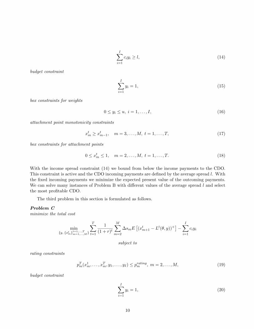
With the income spread constraint (14) we bound from below the income payments to the CDO.This constraint is active and the CDO incoming payments are defined by the average spread l. Withthe fixed incoming payments we minimize the expected present value of the outcoming payments.We can solve many instances of Problem B with different values of the average spread l and selectthe most profitable CDO.

The third problem in this section is formulated as follows.

Problem Cminimize the total cost

min{y, {xtm}

t=1,...,Tm=1,...,M}

T∑t=1

1

(1 + r)t

M∑m=2

∆smE[(xtm+1 − Lt(θ, y))+

]−

I∑i=1

ciyi

subject to

rating constraints

pTm(x1m, . . . , xTm, y1, . . . , yI) ≤ pratingm , m = 2, . . . ,M, (19)

budget constraint

I∑i=1

yi = 1, (20)

10

box constraints for weights

0 ≤ yi ≤ u, i = 1, . . . , I, (21)

attachment point monotonicity constraints

xtm ≥ xtm−1, m = 3, . . . ,M, t = 1, . . . , T, (22)

box constraints for attachment points

0 ≤ xtm ≤ 1, m = 2, . . . ,M, t = 1, . . . , T. (23)

Notice that in Problem C (in contrast to Problem B) the objective is the total cost and there is noincome spread constraint.

2.3 Simplification 1: Problem Decomposition for Large Size Problems.

For a moderate number of scenarios (e.g., 50,000) and a moderate number of instruments (e.g.,200), Problem A can be easily solved with the proposed formulations using PSG [1]. However, forsolving Problem A of a larger size (e.g., 500,000 scenarios), we decompose the problem into M − 1separate sub-problems, i.e., we find the optimal attachment points for each tranche separately andthen combine the solutions. We show further (see proof of Decomposition Theorem in this section)that the following inequality (24) under certain conditions, becomes an equality. Minimum of thesum is always greater than the sum of minimums of its parts, therefore,

min{xtm}

t=1,...,Tm=2,...,M

T∑t=1

1

(1 + r)t

M∑m=1

∆smE[(xtm+1 − Lt)+

]≥

≥M∑m=2

min{xtm}t=1,...,T

T∑t=1

1

(1 + r)t∆sm−1E

[(xtm − Lt)+

]+

T∑t=1

1

(1 + r)t∆sME

[1− Lt

]. (24)

In the inequality (24), we used the fact that xtM+1 = 1. The left hand side of inequality (24) isthe objective of Problem A. To solve Problem A we can solve M − 1 following problems for eachm = 2, . . . ,M .

Problem A(m)minimize present value of expected size of tranche m

min{xtm}t=1,...,T

T∑t=1

1

(1 + r)tE[(xtm − Lt)+

](25)

subject to

11

rating constraint

pTm(x1m, . . . , xTm) ≤ pratingm , (26)

default probability constraints

ptm(x1m, . . . , xtm) ≤ qtm, t = 1, . . . , T − 1 , (27)

box constraints for attachment points

0 ≤ xtm ≤ 1, t = 1, . . . , T , (28)

Notice that we omit the term ∆sm in the objective (25) since it is a fixed nonnegative number,and it does not impact the optimal solution point.

Here is the formal proof that Problem A can be decomposed to Problems A(m), m = 2, . . . ,M .

Decomposition Theorem. If optimal solutions for Problems A(m), m = 2, . . . ,M satisfyinequalities

xtm ≥ xtm−1, m = 3, . . . ,M, t = 1, . . . , T,

then these optimal solutions taken together is the optimal solution of the corresponding Problem A.Proof. Denote the optimal objective values for ProblemsA(m) byAm, and the optimal objective

value for the corresponding Problem A (with the same parameters and data) by A. We can rewrite(24) as

A ≥M∑m=2

Am∆sm +T∑t=1

1

(1 + r)t∆sM+1E

[1− Lt

].

The optimal solutions of Problems A(m) satisfy (5), hence these optimal solutions satisfy all theconstraints (3)-(6). Therefore, these optimal solutions taken together form a feasible point ofProblem A. Hence,

A ≤M∑m=2

Am∆sm +

T∑t=1

1

(1 + r)t∆sM+1E

[1− Lt

].

Consequently,

A =M∑m=2

Am∆sm +T∑t=1

1

(1 + r)t∆sM+1E

[1− Lt

].

and the theorem is proved.

2.4 Simplification 2: Lower and Upper Bounds Minimization.

This section considers a problem of minimizing upper and lower bounds of an objective function inProblem A(m). It shows that the problems of minimizing a lower and upper bounds are equivalent.Using the fact that the cumulative losses Lt are always nonnegative, we can write

xtm ≥ E[(xtm − Lt)+

]≥ E

[xtm − Lt

]= xtm − E

[Lt]

12

for any m = 2, . . . ,M ; t = 1, . . . , T .Thus, the objective in Problem A(m) can be bounded by

T∑t=1

xtm(1 + r)t

≥T∑t=1

1

(1 + r)tE[(xtm − Lt)+

]≥

T∑t=1

xtm(1 + r)t

−T∑t=1

E[Lt]

(1 + r)t. (29)

Since E[Lt]

does not depend on xtm, then the problems of minimizing an upper and lower bounds in(29) are equivalent in the sense that they give the same optimal vectors (although optimal objectivevalues are different).

The objective function can be written as

min{xtm},t=1,...,T

T∑t=1

1

(1 + r)txtm. (30)

We can optimize this objective for either a fixed pool of assets with constraints (3)-(6), or a non-fixed pool of assets with constraints (12)-(18). Our numerical experiments show that there is nosignificant difference between the optimal solutions of Problems A(m) and the optimal solutions ofan upper bound minimization (30). Such a small difference can be explained by the fact that thecumulative CDO losses Lt are usually pretty small compared to xtm. The higher the tranche numberthe closer becomes (xtm − Lt)+ and xtm. The advantage of such simplification is that the nonlinearobjective function of the simplified problem (30) is a linear function of xtm and requires much lesstime to solve compared to the problem with the objective (25). The objective (25) includes partialmoment function E[(xtm−Lt)+], which can be linearized for a discrete number of scenarios. Howeverthis linearization, will lead to a problem of much higher dimension, compared to the problem withsimplified objective (30).

In addition to mathematical expressions we provide further an intuitive explanation that leadsto the same simplification. The higher the rating of the tranche, the lower its spread; therefore, thelarger the size of the highest tranche, the less the cost for the total “insurance”. Thus, we may startfinding the “best” attachment point for the super senior tranche, while maintaining its credit rating.When the attachment point for the super senior tranche is found, one can proceed with the nextlower tranche (suppose it is senior) by solving the same optimization problem for the new rating.Every attachment point that is found serves as a detachment point for the lower tranche. Thus, theattachment points can be obtained recursively for all tranches. Optimizing the single tranche is anindependent problem with the same objective function (30), as soon as higher tranches are fixed.

The problem formulation with the objective (30) is very simple and its solution may be a goodstarting point for the deeper analysis. Therefore, the use of it may provide a preliminary analysison the assets one might want to include in the portfolio.

3 Case Study

This section reports numerical results for several problems described in the previous section. Inparticular, we considered Problem A(m) with objective (25) and simplified objective (30), andProblem B. We solved optimization problems with Portfolio Safeguard (PSG). There are several

13

documented case studies on CDO structuring in the standard version of the PSG package3. Areader may refer to the standard PSG installation to find some other case studies.

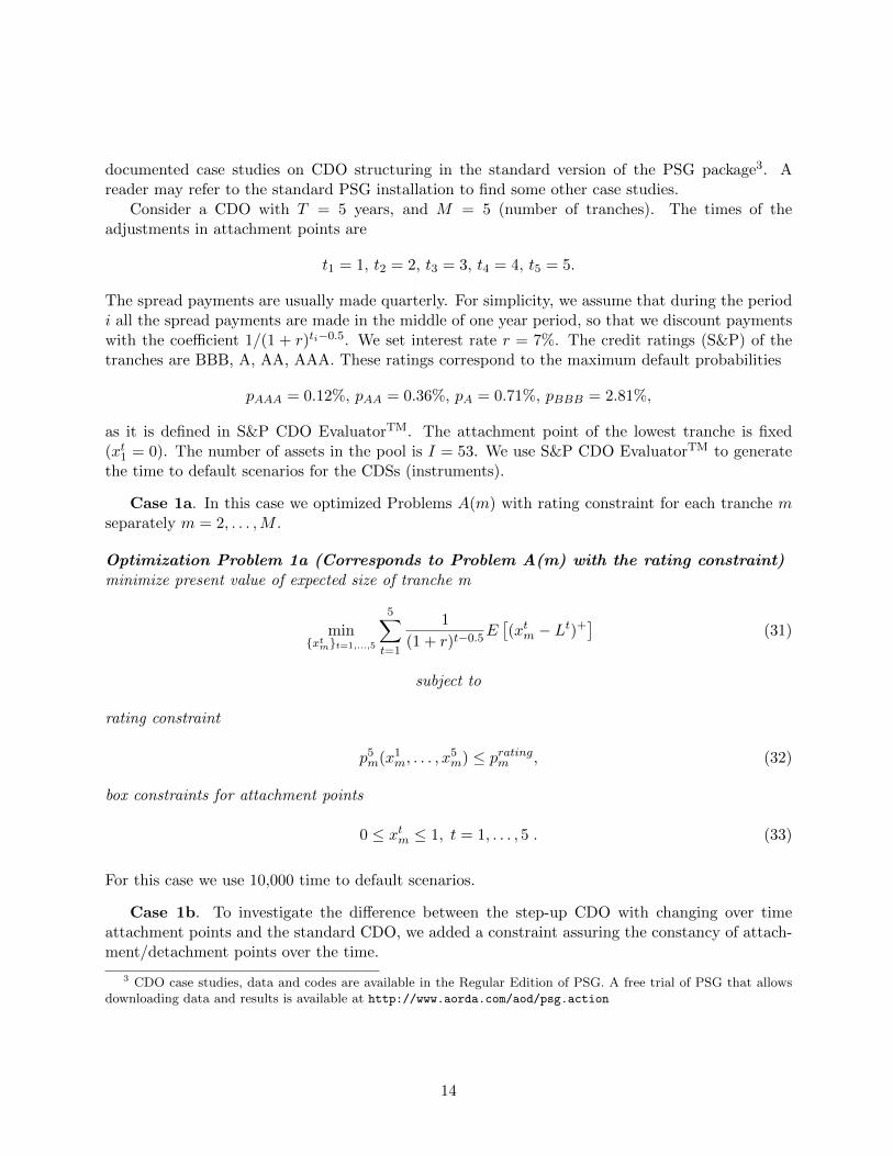
Consider a CDO with T = 5 years, and M = 5 (number of tranches). The times of theadjustments in attachment points are

t1 = 1, t2 = 2, t3 = 3, t4 = 4, t5 = 5.

The spread payments are usually made quarterly. For simplicity, we assume that during the periodi all the spread payments are made in the middle of one year period, so that we discount paymentswith the coefficient 1/(1 + r)ti−0.5. We set interest rate r = 7%. The credit ratings (S&P) of thetranches are BBB, A, AA, AAA. These ratings correspond to the maximum default probabilities

pAAA = 0.12%, pAA = 0.36%, pA = 0.71%, pBBB = 2.81%,

as it is defined in S&P CDO EvaluatorTM. The attachment point of the lowest tranche is fixed(xt1 = 0). The number of assets in the pool is I = 53. We use S&P CDO EvaluatorTM to generatethe time to default scenarios for the CDSs (instruments).

Case 1a. In this case we optimized Problems A(m) with rating constraint for each tranche mseparately m = 2, . . . ,M .

Optimization Problem 1a (Corresponds to Problem A(m) with the rating constraint)minimize present value of expected size of tranche m

min{xtm}t=1,...,5

5∑t=1

1

(1 + r)t−0.5E[(xtm − Lt)+

](31)

subject to

rating constraint

p5m(x1m, . . . , x5m) ≤ pratingm , (32)

box constraints for attachment points

0 ≤ xtm ≤ 1, t = 1, . . . , 5 . (33)

For this case we use 10,000 time to default scenarios.

Case 1b. To investigate the difference between the step-up CDO with changing over timeattachment points and the standard CDO, we added a constraint assuring the constancy of attach-ment/detachment points over the time.

3 CDO case studies, data and codes are available in the Regular Edition of PSG. A free trial of PSG that allowsdownloading data and results is available at http://www.aorda.com/aod/psg.action

14

Optimization Problem 1b (Corresponds to Problem A(m) with rating constraint andattachment point constraints)minimize present value of expected size of tranche m

min{xtm}t=1,...,5

5∑t=1

1

(1 + r)t−0.5E[(xtm − Lt)+

]subject to

rating constraint

p5m(x1m, . . . , x5m) ≤ pratingm , (34)

constancy of attachment points constraint

xtm = xt−1m , t = 2, . . . , 5 , (35)

box constraints for attachment points

0 ≤ xtm ≤ 1, t = 1, . . . , 5 . (36)

Case 2 (Footnote4 provides a link containing data, codes and calculation results for this opti-mization problem). This case considers the difference between the solution of Problem A(m) withthe original objective function (25) and with the simplified objective function (30).

Optimization Problem 2 (Corresponds to Problem A(m) with rating constraint andsimplified objective funtion)minimize simplified objective function of Problem A(m)

min{xtm},t=1,...,5

T∑t=1

1

(1 + r)t−0.5xtm (37)

subject to

rating constraint

p5m(x1m, . . . , x5m) ≤ pratingm , (38)

box constraints for attachment points

0 ≤ xtm ≤ 1, t = 1, . . . , 5 . (39)

4 Data, codes and calculation results for Case 2 with a standard CDO (i.e., with constant over time attach-ment points for BBB tranche can be downloaded from the Web site http://www.aorda.com/aod/casestudy/CS_

Structuring_Step-up_CDO_Optimization_I/problem_example_1_case_2__BBB)

15

Figure 3: Optimization Problems 1a, 1b, 2. Optimal attachment points of 5-period CDO contract.

Tranche rating

Problem 1a

Period BBB A AA AAA

1 0.1491 0.1768 0.1877 0.2258

2 0.1837 0.2147 0.2239 0.2554

3 0.2213 0.2611 0.2722 0.2942

4 0.2604 0.2947 0.3141 0.3307

5 0.2910 0.3342 0.3502 0.3671

Objective 0.5797 0.7261 0.7814 0.8908

Problem 1b

Period BBB A AA AAA

1 - 5 0.2639 0.3043 0.3212 0.3500

Objective 0.7818 0.9524 1.0240 1.1460

Problem 2

Period BBB A AA AAA

1 0.1513 0.1768 0.1877 0.2290

2 0.1816 0.2099 0.2239 0.2554

3 0.2213 0.2652 0.2722 0.2923

4 0.2598 0.3011 0.3141 0.3307

5 0.2910 0.3299 0.3502 0.3671

Figure 3 shows the table with the computational results for Problems 1a, 1b and 2. Thereis a substantial difference between the optimal points and the optimal objectives for optimizationProblems 1a and 1b. The difference between the optimal objectives, for different tranches, is around25%-35% (for instance, for tranche BBB the objective equals 0.5797 for Problem 1a and 0.7818 forProblem 1b). There is a significant difference between spread payments for each tranche in thestep-up CDO and in the standard CDO. The results show that the step-up CDO allows the bankoriginator to save a substantial amount of money. Notice that there is a slight difference betweenthe solutions of Problems 1a and 2 for tranches BBB and A, while solutions for the tranches AAand AAA coincide. This observation has an intuitive interpretation. Simplified objective function(37) in Problem 2 expresses the bank payment if the given tranche does not default. For seniortranches AA and AAA, the default probability is relatively small (less than 0.5%), therefore it isquite reasonable that solutions of Problems 1a and 2 for tranches AA and AAA coincide. Thisobservation justifies the proposed simplified objective (30).

Case 3(Footnote5 provides a link containing data, codes and calculation results for this opti-mization problem). Finally, we simultaneously optimized the CDO portfolio and attachment/de-tachment points with simplified objective (30). For each tranche, m = 2, . . . ,M we optimized the

5Data, codes and calculation results for BBB tranche with l = 0.91% can be downloaded from the Website http://www.aorda.com/aod/casestudy/CS_Structuring_Step-up_CDO_Optimization_II/problem_example_4_

case_1__BBB_91/

16

following problem.

Optimization Problem 3 (Corresponds to Problem B with rating constraint andsimplified objective)minimize present value of size of tranche m

min{xtm,t=1,...,5; y1,...,y53}

T∑t=1

1

(1 + r)t−0.5xtm (40)

subject to

income spread payments constraint

53∑i=1

ciyi ≥ l, (41)

rating constraints

p5m(x1m, . . . , x5m, y1, . . . , y53) ≤ pratingm , m = 2, . . . ,M, (42)

budget constraint

53∑i=1

yi = 1, (43)

box constraints for weights

0 ≤ yi ≤ u, i = 1, . . . , 53, (44)

box constraints for attachment points

0 ≤ xtm ≤ 1, t = 1, . . . , 5 . (45)

The upper bound u was set to u = 2.5%. We considered two different income spread constraints:l = 0.93% and l = 0.97%. Figure 4 shows the table with the results. There is a significant differencebetween the solutions with different income spread payment constraints.

An “efficient frontier” can be created by varying the spread payment constraint l. Then, theparameter l can be selected by maximizing the difference between incoming spread payments l andoutcoming spread payments described by the objectives of optimization problems. PSG meta-codefor Optimization Problem 3 can be found in Appendix 1.

17

Figure 4: Optimization Problem 3. Optimal attachment points of 5-period CDO contract, u = 2.5%,l = 0.93% and 0.97%.

Tranche rating

l=0.93

Period BBB A AA AAA

1 0.1184 0.1388 0.1398 0.1460

2 0.1509 0.1722 0.1829 0.1925

3 0.1896 0.2146 0.2299 0.2445

4 0.2221 0.2545 0.2665 0.2865

5 0.2581 0.2870 0.2938 0.3238

l=0.97

Period BBB A AA AAA

1 0.1616 0.1916 0.2000 0.1989

2 0.1991 0.2416 0.2500 0.2489

3 0.2491 0.2783 0.3000 0.3229

4 0.2866 0.3283 0.3416 0.3729

5 0.3241 0.3616 0.3666 0.4229

4 Conclusion

The paper considered an optimization framework for structuring CDOs. Three optimization modelswere developed from a bank originator prospective. With the first model we optimized only attach-ment/detachment points in a CDO: the goal was to minimize payments for the credit risk protection(premium leg), while maintaining credit rating of tranches. In this case the pool of CDSs and incomespreads were fixed. With the second model, we bounded from below the total income spread pay-ments and optimized the set of CDSs in a CDO pool and the attachment/detachment points. Withthe third model, we minimized the difference between the total outcome and income spreads. Wesimultaneously optimized the set of CDSs in a CDO pool and the attachment/detachment points,while maintaining specific credit rating of tranches.

Case Study section presented numerical results for Problem A(m) and Problem B, discussedin this paper. We compared results for the step-up CDO (Problem 1a) and the standard CDO(Problem 1b). The difference between the expected payments for tranches was around 25%− 35%.Also, we investigated a step-up CDO with original and simplified objectives (Problem 2). Weobserved that there is only a slight difference between optimal points corresponding to the step-up CDO with the original objective (Problem 1a) and simplified objective (Problem 2). Finallywe simultaneously optimized the CDO pool and attachment/detachment points for two differentincome spread payment constraints (Problem 3). There was a significant difference in solutions withdifferent income spread payment constraints.

References

[1] Portfolio safeguard, version 2.1. http://www.aorda.com/aod/welcome.action, 2008.

18

[2] M. Choudhry. Structured Credit Products: Credit Derivatives and Synthetic Securitisation.Wiley Finance. John Wiley & Sons, 2010.

[3] S. Das. Credit derivatives: CDOs and structured credit products. Wiley finance series. JohnWiley & Sons (Asia), 2005.

[4] I. Halperin. Implied multi-factor model for bespoke cdo tranches and other portfolio creditderivatives. Quantitative research, JP Morgan, 2009.

[5] J. Hull and A. White. An improved implied copula model and its application to the valuationof bespoke cdo tranches. Journal of Investment Management, June 2009.

[6] D. Jewan, R. Guo, and G. Witten. Optimal bespoke cdo design via nsga-ii. Journal of AppliedMathematics and Decision Sciences, 2009, 2009.

[7] B.P. Lancaster, G.M. Schultz, and CFA Frank J. Fabozzi. Structured Products and RelatedCredit Derivatives: A Comprehensive Guide for Investors. Frank J. Fabozzi Series. Wiley, 2008.

[8] A. Rajan, G. McDermott, and R. Roy. The Structured Credit Handbook. Wiley Finance. Wiley,2007.

[9] D. Rosen and D. Saunders. Valuing cdos of bespoke portfolios with implied multi-factor models.Journal of Credit Risk, 5(3):3–36, Feb. 2009.

Appendix 1: Portfolio Safeguard (PSG) Example Code

This appendix presents the PSG meta-code for solving Optimization Problem 3, see formulas(40)− (45). Meta-code, Data and Solutions can be downloaded from the link6.

Meta-Code for Optimization Problem 31 Problem: problem example 4 case 1 BBB 91, type = minimize2 Objective: objective linear sum of x 5, linearize = 03 linear sum of x 5(matrix sum of x 5)4 Constraint: constraint mult prob BBB, upper bound = 0.02815 prmulti pen 5 periods(0.00000000,matrix 4 1,matrix 4 2,

matrix 4 3,matrix 4 4,matrix 4 5)6 Constraint: constraint spread, lower bound = 91, linearize = 07 linear spread(matrix spread)8 Constraint: constraint budget, lower bound = 1, upper bound = 1, linearize = 09 linear budget(matrix budget)10 Box of Variables: lowerbounds = point lowerbounds, upperbounds = point upperbounds11 Solver: VAN, precision = 2, stages = 6

Here we give a brief description of the presented meta-code. We boldfaced the important partsof the code. The keyword minimize tells a solver that Problem 3 is a minimization problem. To

6http://www.ise.ufl.edu/uryasev/research/testproblems/financial_engineering/

structuring-step-up-cdo/ , Problem 6, Data Set 2

19

define an objective function the keyword Objective is used. The linear objective function (40),that is the present value of expected size of a tranche, is defined in lines 2,3 with the keyword linearand the data matrix located in the file matrix sum of x 5.txt. Each constraint starts from thekeyword Constraint. The rating constraint (42) is defined in lines 4,5. In PSG, the keywordprmulti pen denotes the probability that a system of linear equations with random coefficients issatisfied (see the mathematical definition of function prmulti pen in the document7). The randomcoefficients for four linear inequalities are given by four matrices of scenarios in the following fourfiles, matrix 4 1.txt,. . . ,matrix 4 4.txt. The income spread payment constraint (41) and budgetconstraint (43) are defined with linear functions in lines 6,7 and 7-8 accordingly, similar to theobjective function.

7 http://www.ise.ufl.edu/uryasev/files/2011/12/definitions_of_functions.pdf, page 104

20