Optimal Stops and Algorithmic Trading - Welcome …...Optimal Stops and Algorithmic Trading Giuseppe...
33
Optimal Stops and Algorithmic Trading Giuseppe Di Graziano [email protected] November 20, 2013 Giuseppe Di Graziano (Deutsche Bank-KCL) Optimal Stops and Algorithmic Trading November 20, 2013 1 / 33
Transcript of Optimal Stops and Algorithmic Trading - Welcome …...Optimal Stops and Algorithmic Trading Giuseppe...
Optimal Stops and Algorithmic Trading
Giuseppe Di Graziano
November 20, 2013
Giuseppe Di Graziano (Deutsche Bank-KCL) Optimal Stops and Algorithmic Trading November 20, 2013 1 / 33
Overview
1 Motivation and Set Up
2 Optimal Stops with Constant P&L Drift
3 Optimal Stops with Unknown P&L Drift
4 Optimal Stops with Stochastic Drift
5 Numerical Examples
6 Calibration
Giuseppe Di Graziano (Deutsche Bank-KCL) Optimal Stops and Algorithmic Trading November 20, 2013 2 / 33
Motivation
Stop loss and target profit thresholds are commonly used bypractitioners
Intuitively they must be related to the risk preferences of theindividual trader/desk
They must also depend on the track record of a given trader/strategy
We propose approach which allows to link the risk preferences of thetrader to the characteristics of a given strategy in an algorithmiccontext
Giuseppe Di Graziano (Deutsche Bank-KCL) Optimal Stops and Algorithmic Trading November 20, 2013 3 / 33
Set Up
Underlying: single asset, time spreads, inter asset spreads, basket ofassets
When a position is entered a fixed number of contracts N isbought/sold
When a position is exited all the outstanding N contracts aresold/bought back
Giuseppe Di Graziano (Deutsche Bank-KCL) Optimal Stops and Algorithmic Trading November 20, 2013 4 / 33
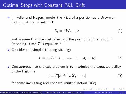
Optimal Stops with Constant P&L Drift
[Imkeller and Rogers] model the P&L of a position as a Brownianmotion with constant drift
Xt = σWt + µt (1)
and assume that the cost of exiting the position at the random(stopping) time T is equal to c
Consider the simple stopping strategy
T ≡ inf {t : Xt = −a or Xt = b} (2)
One approach to the exit problem is to maximise the expected utilityof the P&L, i.e.
φ = E [e−ρTU(XT − c)] (3)
for some increasing and concave utility function U(x)
Giuseppe Di Graziano (Deutsche Bank-KCL) Optimal Stops and Algorithmic Trading November 20, 2013 5 / 33
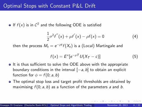
Optimal Stops with Constant P&L Drift
If f (x) is in C2 and the following ODE is satisfied
1
2σ2f
′′(x) + µf
′(x)− ρf (x) = 0 (4)
then the process Mt = e−ρt f (Xt) is a (Local) Martingale and
f (x) = E x [e−ρTU(XT − c)] (5)
It is thus sufficient to solve the ODE above with the appropriateboundary conditions in the interval [−a, b] to obtain an explicitfunction for φ = f (0; a, b)
The optimal stop loss and target profit thresholds are obtained bymaximising f (0; a, b) as a function of the parameters a and b.
Giuseppe Di Graziano (Deutsche Bank-KCL) Optimal Stops and Algorithmic Trading November 20, 2013 6 / 33
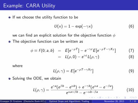
Example: CARA Utility
If we choose the utility function to be
U(x) = 1− exp(−γx) (6)
we can find an explicit solution for the objective function φ
The objective function can be written as
φ ≡ f (0; a, b) = E [e−ρT ]− e−γcE [e−ρT−γXT ] (7)
= L(ρ, 0)− eγcL(ρ, γ) (8)
whereL(ρ, γ) = E [e−ρT−γXT ] (9)
Solving the ODE, we obtain
L(ρ, γ) =eγa(eβb − eαb) + e−γb(eαa − e−βa)
eαa+βb − e−αb−βa(10)
Giuseppe Di Graziano (Deutsche Bank-KCL) Optimal Stops and Algorithmic Trading November 20, 2013 7 / 33
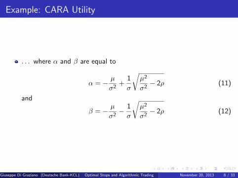
Example: CARA Utility
. . . where α and β are equal to
α = − µ
σ2+
1
σ
õ2
σ2− 2ρ (11)
and
β = − µ
σ2− 1
σ
õ2
σ2− 2ρ (12)
Giuseppe Di Graziano (Deutsche Bank-KCL) Optimal Stops and Algorithmic Trading November 20, 2013 8 / 33
Optimal Stops with Unknown P&L Drift
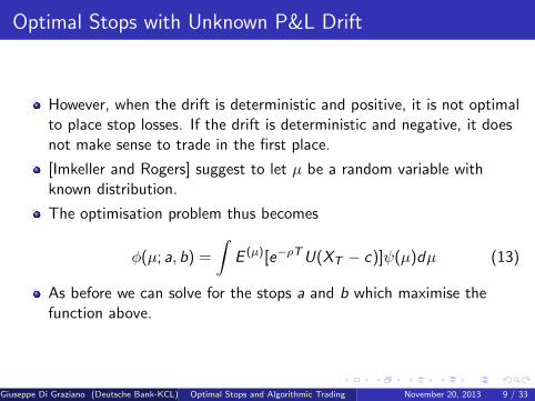
However, when the drift is deterministic and positive, it is not optimalto place stop losses. If the drift is deterministic and negative, it doesnot make sense to trade in the first place.
[Imkeller and Rogers] suggest to let µ be a random variable withknown distribution.
The optimisation problem thus becomes
φ(µ; a, b) =
∫E (µ)[e−ρTU(XT − c)]ψ(µ)dµ (13)
As before we can solve for the stops a and b which maximise thefunction above.
Giuseppe Di Graziano (Deutsche Bank-KCL) Optimal Stops and Algorithmic Trading November 20, 2013 9 / 33
Optimal Stops with Stochastic Drift
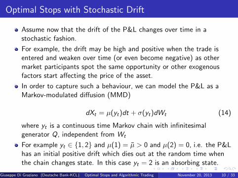
Assume now that the drift of the P&L changes over time in astochastic fashion.
For example, the drift may be high and positive when the trade isentered and weaken over time (or even become negative) as othermarket participants spot the same opportunity or other exogenousfactors start affecting the price of the asset.
In order to capture such a behaviour, we can model the P&L as aMarkov-modulated diffusion (MMD)
dXt = µ(yt)dt + σ(yt)dWt (14)
where yt is a continuous time Markov chain with infinitesimalgenerator Q, independent from Wt
For example yt ∈ {1, 2} and µ(1) = µ > 0 and µ(2) = 0, i.e. the P&Lhas an initial positive drift which dies out at the random time whenthe chain changes state. In this case yt = 2 is an absorbing state.
Giuseppe Di Graziano (Deutsche Bank-KCL) Optimal Stops and Algorithmic Trading November 20, 2013 10 / 33
Optimal Stops with Stochastic Drift
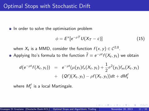
In order to solve the optimisation problem
φ = E x [e−ρTU(XT − c)] (15)
when Xt is a MMD, consider the function f (x , y) ∈ C2,0.
Applying Ito’s formula to the function f ≡ e−ρt f (Xt , yt) we obtain
d(e−ρt f (Xt , yt)) = e−ρt(µ(yt)fx(Xt , yt) +1
2σ2(yt)fxx(Xt , yt)
+ (Qf )(Xt , yt)− ρf (Xt , yt))dt + dM ft
where M ft is a local Martingale.
Giuseppe Di Graziano (Deutsche Bank-KCL) Optimal Stops and Algorithmic Trading November 20, 2013 11 / 33
Optimal Stops with Stochastic Drift
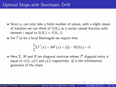
Since yt can only take a finite number of values, with a slight abuseof notation we can think of f (Xt) as a vector valued function withelement i equal to fi (Xt) ≡ f (Xt , i)
For f to be a local Martingale we require that
1
2Σf
′′(x) + Mf
′(x) + (Q − R)f (x) = 0
Here Σ, M and R are diagonal matrices whose ith diagonal entry isequal to σ(i), µ(i) and ρ(i) respectively. Q is the infinitesimalgenerator of the chain.
Giuseppe Di Graziano (Deutsche Bank-KCL) Optimal Stops and Algorithmic Trading November 20, 2013 12 / 33
Optimal Stops with Stochastic Drift
Since f (x) is bounded in the interval [−a, b], it follows from theoptional stopping theorem that
fi (x) = E x ,i [e−ρTU(XT − c)]
where y0 = i is the initial state of the chain and we have used theboundary conditions{fi (−a) = U(−a− c) i ∈ {1, . . . , n}fi (b) = U(b − c) i ∈ {1, . . . , n}
Giuseppe Di Graziano (Deutsche Bank-KCL) Optimal Stops and Algorithmic Trading November 20, 2013 13 / 33
Optimal Stops with Stochastic Drift
The system of ODEs above admits solutions of the form
f (x) = ve−λx (16)
where v is a n dimensional vector
Substituting (16) into the system (12) and re-arranging we obtain
λ2v − 2λΣ−1Mv + 2Σ−1(Q − R)v = 0
The quadratic eigenvalue problem (14) can be reduced to a canonicaleigenvalue problem 2Σ−1M −2Σ−1(Q − R)
I 0
( hv
)= λ
(hv
)where
h = λv
Giuseppe Di Graziano (Deutsche Bank-KCL) Optimal Stops and Algorithmic Trading November 20, 2013 14 / 33
Optimal Stops with Stochastic Drift
This is a standard eigenvalue problem which admits n solutions in thepositive half plane and n in the negative half plane
The solution to our ODE system will thus take the form
f (x) =2n∑i=1
wivie−λix
The 2n coefficients wi can be derived by solving the system{∑2ni=1 wivie
−λib = U(b − c)∑2ni=1 wivie
λia = U(−a− c)
Here U(z) is an n dimensional vector with ith entry equal to U(z).
Giuseppe Di Graziano (Deutsche Bank-KCL) Optimal Stops and Algorithmic Trading November 20, 2013 15 / 33
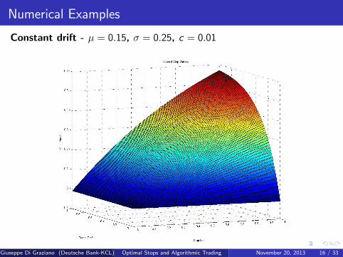
Numerical Examples
Constant drift - µ = 0.15, σ = 0.25, c = 0.01
Giuseppe Di Graziano (Deutsche Bank-KCL) Optimal Stops and Algorithmic Trading November 20, 2013 16 / 33
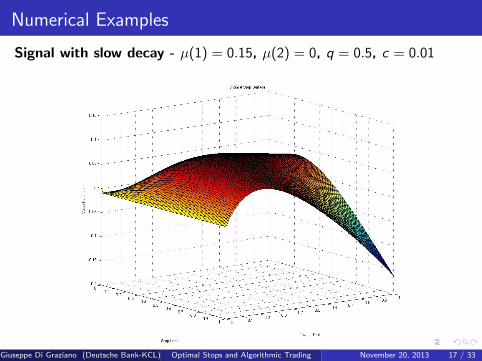
Numerical Examples
Signal with slow decay - µ(1) = 0.15, µ(2) = 0, q = 0.5, c = 0.01
Giuseppe Di Graziano (Deutsche Bank-KCL) Optimal Stops and Algorithmic Trading November 20, 2013 17 / 33
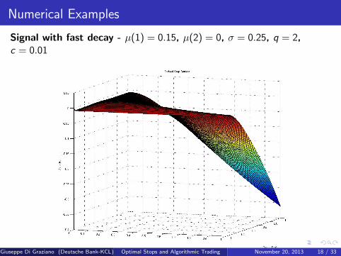
Numerical Examples
Signal with fast decay - µ(1) = 0.15, µ(2) = 0, σ = 0.25, q = 2,c = 0.01
Giuseppe Di Graziano (Deutsche Bank-KCL) Optimal Stops and Algorithmic Trading November 20, 2013 18 / 33
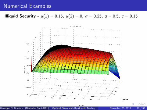
Numerical Examples
Illiquid Security - µ(1) = 0.15, µ(2) = 0, σ = 0.25, q = 0.5, c = 0.15
Giuseppe Di Graziano (Deutsche Bank-KCL) Optimal Stops and Algorithmic Trading November 20, 2013 19 / 33
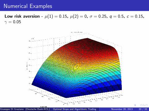
Numerical Examples
Low risk aversion - µ(1) = 0.15, µ(2) = 0, σ = 0.25, q = 0.5, c = 0.15,γ = 0.05
Giuseppe Di Graziano (Deutsche Bank-KCL) Optimal Stops and Algorithmic Trading November 20, 2013 20 / 33
Numerical Examples
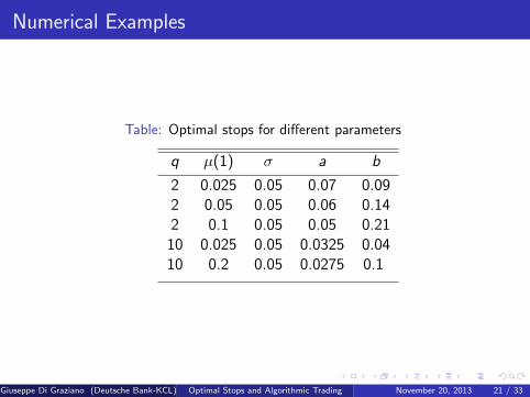
Table: Optimal stops for different parameters
q µ(1) σ a b
2 0.025 0.05 0.07 0.092 0.05 0.05 0.06 0.142 0.1 0.05 0.05 0.21
10 0.025 0.05 0.0325 0.0410 0.2 0.05 0.0275 0.1
Giuseppe Di Graziano (Deutsche Bank-KCL) Optimal Stops and Algorithmic Trading November 20, 2013 21 / 33
Calibration
In the simple model of the example above, calibration can be carriedout analytically
For the calibration to be reliable a relatively high number of backtestsare necessary, which is possible in the high frequency domain
The volatility σ can calculated using standard methods
The cost c can be easily be estimated using bid-ask data
Giuseppe Di Graziano (Deutsche Bank-KCL) Optimal Stops and Algorithmic Trading November 20, 2013 22 / 33
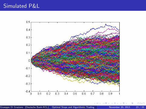
Simulated P&L
Giuseppe Di Graziano (Deutsche Bank-KCL) Optimal Stops and Algorithmic Trading November 20, 2013 23 / 33
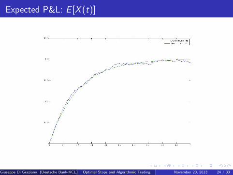
Expected P&L: E [X (t)]
Giuseppe Di Graziano (Deutsche Bank-KCL) Optimal Stops and Algorithmic Trading November 20, 2013 24 / 33
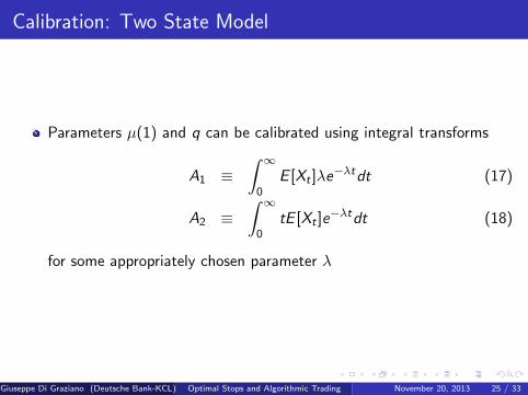
Calibration: Two State Model
Parameters µ(1) and q can be calibrated using integral transforms
A1 ≡∫ ∞
0E [Xt ]λe
−λtdt (17)
A2 ≡∫ ∞
0tE [Xt ]e
−λtdt (18)
for some appropriately chosen parameter λ
Giuseppe Di Graziano (Deutsche Bank-KCL) Optimal Stops and Algorithmic Trading November 20, 2013 25 / 33
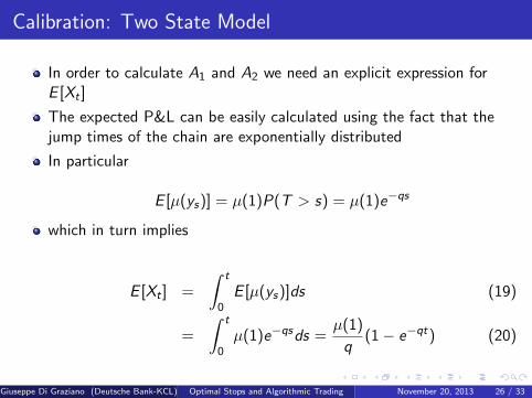
Calibration: Two State Model
In order to calculate A1 and A2 we need an explicit expression forE [Xt ]
The expected P&L can be easily calculated using the fact that thejump times of the chain are exponentially distributed
In particular
E [µ(ys)] = µ(1)P(T > s) = µ(1)e−qs
which in turn implies
E [Xt ] =
∫ t
0E [µ(ys)]ds (19)
=
∫ t
0µ(1)e−qsds =
µ(1)
q(1− e−qt) (20)
Giuseppe Di Graziano (Deutsche Bank-KCL) Optimal Stops and Algorithmic Trading November 20, 2013 26 / 33
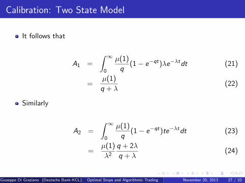
Calibration: Two State Model
It follows that
A1 =
∫ ∞0
µ(1)
q(1− e−qt)λe−λtdt (21)
=µ(1)
q + λ(22)
Similarly
A2 =
∫ ∞0
µ(1)
q(1− e−qt)te−λtdt (23)
=µ(1)
λ2
q + 2λ
q + λ(24)
Giuseppe Di Graziano (Deutsche Bank-KCL) Optimal Stops and Algorithmic Trading November 20, 2013 27 / 33
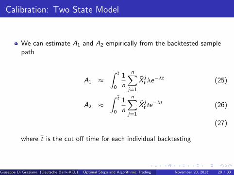
Calibration: Two State Model
We can estimate A1 and A2 empirically from the backtested samplepath
A1 ≈∫ t
0
1
n
n∑j=1
X jtλe−λt (25)
A2 ≈∫ t
0
1
n
n∑j=1
X jt te−λt (26)
(27)
where t is the cut off time for each individual backtesting
Giuseppe Di Graziano (Deutsche Bank-KCL) Optimal Stops and Algorithmic Trading November 20, 2013 28 / 33
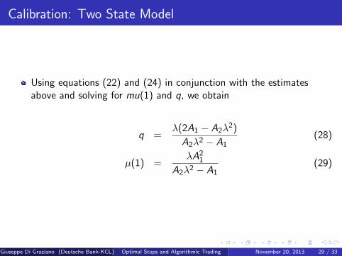
Calibration: Two State Model
Using equations (22) and (24) in conjunction with the estimatesabove and solving for mu(1) and q, we obtain
q =λ(2A1 − A2λ
2)
A2λ2 − A1(28)
µ(1) =λA2
1
A2λ2 − A1(29)
Giuseppe Di Graziano (Deutsche Bank-KCL) Optimal Stops and Algorithmic Trading November 20, 2013 29 / 33
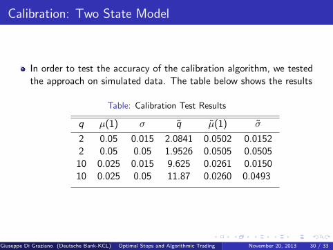
Calibration: Two State Model
In order to test the accuracy of the calibration algorithm, we testedthe approach on simulated data. The table below shows the results
Table: Calibration Test Results
q µ(1) σ q µ(1) σ
2 0.05 0.015 2.0841 0.0502 0.01522 0.05 0.05 1.9526 0.0505 0.0505
10 0.025 0.015 9.625 0.0261 0.015010 0.025 0.05 11.87 0.0260 0.0493
Giuseppe Di Graziano (Deutsche Bank-KCL) Optimal Stops and Algorithmic Trading November 20, 2013 30 / 33
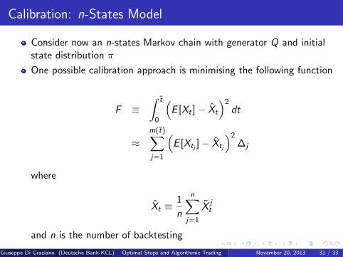
Calibration: n-States Model
Consider now an n-states Markov chain with generator Q and initialstate distribution π
One possible calibration approach is minimising the following function
F ≡∫ t
0
(E [Xt ]− Xt
)2dt
≈m(t)∑j=1
(E [Xtj ]− Xtj
)2∆j
where
Xt ≡1
n
n∑j=1
X jt
and n is the number of backtesting
Giuseppe Di Graziano (Deutsche Bank-KCL) Optimal Stops and Algorithmic Trading November 20, 2013 31 / 33
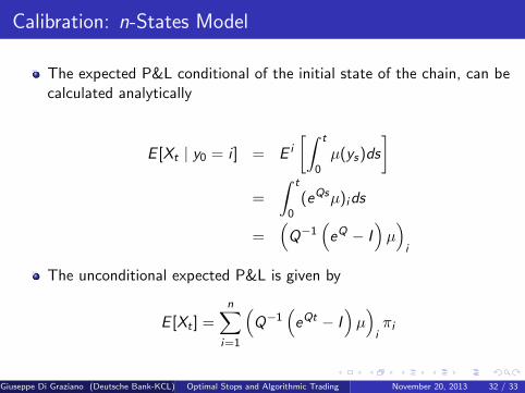
Calibration: n-States Model
The expected P&L conditional of the initial state of the chain, can becalculated analytically
E [Xt | y0 = i ] = E i
[∫ t
0µ(ys)ds
]=
∫ t
0(eQsµ)ids
=(Q−1
(eQ − I
)µ)i
The unconditional expected P&L is given by
E [Xt ] =n∑
i=1
(Q−1
(eQt − I
)µ)iπi
Giuseppe Di Graziano (Deutsche Bank-KCL) Optimal Stops and Algorithmic Trading November 20, 2013 32 / 33
References
Imkeller and Rogers (2011)
Trading to Stop Working Paper, University of Cambridge
Di Graziano and Rogers (2005)
Barrier option pricing for assets with Markov-modulated dividends Journal ofComputational Finance, 9, 75-87
Giuseppe Di Graziano (Deutsche Bank-KCL) Optimal Stops and Algorithmic Trading November 20, 2013 33 / 33