Optimal Shape Design in MagnetostaticsPhd
165
V ˇ SB–Technical University of Ostrava Faculty of Electrical Engineering and Computer Science Department of Applied Mathematics Optimal Shape Design in Magnetostatics Ph.D. Thesis Author: Ing. Dalibor Luk´ aˇ s Supervisor: Prof. RNDr. Zdenˇ ek Dost´ al, CSc. Department of Applied Mathematics, V ˇ SB–Technical University of Ostrava Referees: Prof. RNDr. Jaroslav Haslinger, DrSc. Faculty of Mathematics and Physics, Charles University Prague Prof. RNDr. Michal Kˇ r´ ıˇ zek, DrSc. Mathematical Institute, The Academy of Sciences of the Czech Republic o.Univ.Prof. Dipl.-Ing. Dr. Ulrich Langer Institute of Computational Mathematics, Johannes Kepler University Linz Submitted in September 2003
-
Upload
mmahdiroodi -
Category
Documents
-
view
27 -
download
0
description
Optimal Shape Design in Magnetostatics PhD Thesis by Ing. Dalibor Luk ´ aˇ
Transcript of Optimal Shape Design in MagnetostaticsPhd
VSB–Technical University of Ostrava
Faculty of Electrical Engineering and Computer Science
Department of Applied Mathematics
Optimal Shape Design in Magnetostatics
Ph.D. Thesis
Author: Ing. Dalibor Lukas
Supervisor: Prof. RNDr. Zdenek Dostal, CSc.Department of Applied Mathematics,
VSB–Technical University of Ostrava
Referees: Prof. RNDr. Jaroslav Haslinger, DrSc.Faculty of Mathematics and Physics,Charles University Prague
Prof. RNDr. Michal Krızek, DrSc.Mathematical Institute,The Academy of Sciences of the Czech Republic
o.Univ.Prof. Dipl.-Ing. Dr. Ulrich LangerInstitute of Computational Mathematics,Johannes Kepler University Linz
Submitted in September 2003


VSB–Technical University of Ostrava
Faculty of Electrical Engineering and Computer Science
Department of Applied Mathematics
Optimal Shape Design in Magnetostatics
Ph.D. Thesis
September 2003 Ing. Dalibor Lukas


Dedicated to Sarka

iv

Abstract
This thesis treats with theoretical and computational aspects of three–dimensional optimal shapedesign problems that are governed by linear magnetostatics. The aim is to present a completeprocess of mathematical modelling in a well–balanced way. We step–by–step visit the worldof physics, functional analysis, computational mathematics, and we end up with real–life applica-tions. Nevertheless, the main emphasis is put on an efficient implementation of numerical methodsfor shape optimization which exploits an effective evaluation of gradients by the adjoint methodand a just recently introduced multilevel optimization approach. We also emphasize numericalexperiments with real–life problems of complex three–dimensional geometries.
We begin from a description of the electromagnetic phenomena by Maxwell’s equations andwe derive their three–dimensional (3d) and two–dimensional (2d) magnetostatic cases with thelinear constitutive relation between the magnetic flux density and the magnetic strength density.
Then we start to develop a general theory that covers both 2d and 3d optimal interface–shapedesign problems that are constrained by a second–order linear elliptic boundary vector–value prob-lem (BVP). First we pose a weak formulation of the BVP with the homogeneous Dirichlet bound-ary condition. Whenever the kernel of the BVP operator is not trivial, we employ a regularizationtechnique such that the regularized solutions converge to the true one. The continuous weak for-mulation of the abstract BVP is discretized by the first–order finite element method on trianglesand tetrahedra, respectively. We set an abstract continuous shape optimization problem, the stateproblem of which involves one or more BVPs such that they only differ in the right–hand sides,i.e., different current excitations in case of magnetostatics. The design boundary is an interfacebetween two materials, rather than a part of the computational domain boundary, as it is usual inoptimal shape design for mechanics. We prove the existence of an optimal shape by checking thecontinuity of the cost functional and the compactness of the set of admissible shapes. Then we dis-cretize the continuous optimization problem by the finite element method and prove the existenceof the approximate solutions. The main theoretical result of this thesis is a proof of the conver-gence of the approximate optimized solutions to an optimal solution of the continuous problem,where we also involve an inner approximation of the original computational domain with a Lips-chitz boundary by a polyhedral (in the 3d case) or polygonal (in the 2d case) domain. Throughoutthe abstract theory we introduce many assumptions that are checked for concrete applicationsafterwards. These assumptions show the scope of the theory.
Concerning the computational aspects in optimization, we use the sequential quadratic pro-gramming method with a successive approximation of the Hessian. To justify the use, we verifythe smoothness of both the discretized cost and constraint functionals. Then we focus on thecalculation of gradients by means of the adjoint method and we derive an efficient algorithm forthat, including its Matlab implementation enclosed on the CD. We introduce a new multileveloptimization approach as a possible adaptive optimization method.
Finally, we end up with physics again. We present two real–life applications with rather com-
v

vi ABSTRACT
plex 3d geometries. After some motivation, we describe the optimization problem in terms ofverifying the theoretical assumptions, and we give numerical results. We present the speedupof the adjoint method comparing to the numerical differentiation, and of the multilevel approachcomparing to the classical optimization. One optimized design was manufactured, we are providedwith measurements and, at the end, we discuss real improvements of the cost functional.
Acknowledgement
First of all I want to express my deep gratitude to my supervisor Prof. RNDr. Zdenek Dostal, CSc.,the head of the Department of Applied Mathematics at the Technical University of Ostrava (TUO),who introduced me to the magic of numerical mathematics and its applications in electromag-netism. I thank him for his kindness and patience during more than six years of my undergraduateand doctoral studies for when he has been supervising me.
Special thanks are devoted to my very good friend, teacher, and colleague Doc. RNDr. JirıBouchala, Ph.D., who is an associated professor at the Department of Applied Mathematics, TUO.Jirka convinced me that the mathematics is beautiful itself, even without applications. I thank to allthe other friends, colleagues, and teachers of mine from the Department of Applied Mathematics,TUO, especially to Mgr. Vıt Vondrak, Ph.D. and Mgr. Bohumil Krajc, Ph.D.
I am much obliged to o.Univ.Prof. Dipl.-Ing. Dr. Ulrich Langer, who is the head of the Institutefor Numerical Mathematics and the co–speaker of the Special Research Initiative SFB F013 “Nu-merical and Symbolic Scientific Computing” both associated to the Johannes Kepler UniversityLinz in Austria. Professor Langer offered me a Ph.D. position within the research project SFBF013, where I spent one year and where I have been currently working again. Here I have madea big progress in my research work and I have learned about efficient methods for solving largediscretized direct simulation problems based on the finite element and/or boundary element dis-cretizations. I am also much indebted to my current or former colleagues, especially, I would liketo mention Dr. Dipl.-Ing. Joachim Schoberl, Dr. Dipl.-Ing. Michael Kuhn, MSc., and Dr. Dipl.-Ing. Wolfram Muhlhuber.
I further thank to Prof. Ing. Jaromır Pistora, CSc., who is with the Institute of Physics, TUO,and is the head of the Department of Education at the Faculty of Electrical Engineering. ProfessorPistora asked me to cooperate on development of a new generation of electromagnets used in theresearch on magnetooptic effects. I also thank for the fruitful cooperation to the other colleaguesfrom the Institute of Physics, namely to Dr. Mgr. Kamil Postava, Dr. RNDr. Dalibor Ciprian,Dr. Ing. Michal Lesnak, Ing. Martin Foldyna, and Ing. Igor Kopriva.
I very appreciate the possibility to consult my work with Prof. RNDr. Jaroslav Haslinger, DrSc.,who is a world leading expert in optimal shape design. I thank very much to Prof. RNDr. MichalKrızek, DrSc. from the Mathematical Institute of the Czech Academy of Sciences that I could learna lot during several consultations in his office. I very much admire the enthusiasm of Prof. Krızekthat he has devoted to math.
At the end let me express my deep grateness and love to my parents and to my girlfriend Sarka,with whom my life is complete, no matter what the career is about.
This work has been supported by the Austrian Science Fund FWF within the SFB “Numerical andSymbolic Computing” under the grant SFB F013, by the Czech Ministry of Education under theresearch project CEZ: J17/98:272400019, and by the Grant Agency of the Czech Republic underthe grant 105/99/1698.
vii

viii ACKNOWLEDGEMENT

Notation
N non–negative integersR real numbersi imaginary unitC complex planeC1, . . . , C16 fixed constants
Abbreviations
1d one–dimensional2d two–dimensional3d three–dimensionalPDE partial differential equationBVP boundary (vector–)value problemFEM finite element methodBFGS update formula for the Hessian matrix named after Broyden,
Fletcher, Goldfarb, and ShannoSQP sequential quadratic programmingAD automatic differentiation
Chapter 2
B magnetic flux density p. 10H magnetic field p. 10µ permeability p. 10J direct electric current density p. 10u magnetic vector potential p. 10Ω three–dimensional computational domain p. 10Ω2d two–dimensional reduced computational domain which is the
cross section of Ω with the plane x3 = 0p. 11
J two–dimensional scalar direct electric current density p. 11u two–dimensional scalar magnetic potential p. 11
Chapter 3
‖ · ‖U norm in the normed linear vector space U p. 14V/U quotient space p. 14Ker(L) kernel of the linear vector operator L p. 15U ′ dual space to the normed linear vector space U p. 15〈·, ·〉 duality pairing p. 15(·, ·) scalar product p. 15
ix

x NOTATION
U⊥ orthogonal complement to the space U p. 16H = U ⊕ U⊥ orthogonal decomposition of the Hilbert space H p. 17Rn Euclidean space consisting of n–dimensional real vectors p. 17AT transposed matrix p. 18det(A) determinant of the matrix A p. 18A adjoint matrix p. 18A−1 inverse matrix p. 18m dimension of the computational domain Ω, m ∈ 2, 3 p. 19Ω domain, i.e., open, bounded, and connected subset of Rm p. 19Ω closure of the domain Ω p. 19∂Ω boundary of the domain Ω p. 19n unit outer normal vector to the boundary ∂Ω p. 19C(Ω) space of functions continuous over Ω p. 20Ck(Ω) space of functions which are continuous up to their k–th partial
derivatives over Ω, k ∈ N
p. 20
C∞(Ω) space of infinitely differentiable functions over Ω p. 21suppv support of the function v p. 21C∞
0 (Ω) space of infinitely differentiable functions with a compact supportin Ω
p. 21
C0,1(Ω) space of Lipschitz continuous functions over Ω p. 21L set of all the domains with Lipschitz continuous boundaries p. 21div divergence operator p. 22grad gradient operator p. 22curl curl operator p. 22n× u cross product, tangential component of the function u along the
boundary ∂Ωp. 23
B linear vector first–order differential operator, B :[C1(Ω)
]ν1 7→[C(Ω)
]ν2 , ν1, ν2 ∈ N
p. 23
B∗ adjoint operator related to B by Green’s theorem, B :[C1(Ω)
]ν2 7→[C(Ω)
]ν1
p. 23
γ trace operator related to B by Green’s theorem, γ :[C(Ω)
]ν1 7→[C(∂Ω)]ν2
p. 23
Lp(Ω) Lebesgue space of measurable functions defined over Ω for whichthe Lebesgue integral of their p–th power is finite, p ∈ [1,∞)
p. 24
L∞(Ω) Lebesgue space of measurable essentially bounded functions overΩ
p. 24
meas(Ω) Lebesgue measure of the domain Ω p. 24a.e. almost everywhere p. 24Dαu the α–th generalized derivative of the function u, α is a multi–
indexp. 25
Hk(Ω) Sobolev space of functions whose generalized derivatives up tothe k–th order belong to Lp(Ω)
p. 25
(·, ·)k,Ω scalar product in Hk(Ω) p. 25‖ · ‖k,Ω norm in Hk(Ω) p. 25| · |k,Ω seminorm in Hk(Ω) p. 25[Hk(Ω)
]nCartesian product of Sobolev spaces, n ∈ N p. 25
(·, ·)n,k,Ω scalar product in[Hk(Ω)
]np. 25
H10 (Ω) space of functions from H1(Ω) whose traces vanish along ∂Ω p. 26
xi
H1/2(∂Ω) space of traces of all functions from H1(Ω) p. 26H−1/2(∂Ω) dual space to H1/2(∂Ω) p. 26H(B; Ω) space of functions from
[L2(Ω)
]ν1 whose generalized operator B
(gradient, divergence, curl, etc.) is in[L2(Ω)
]ν2
p. 30
(·, ·)B,Ω scalar product in H(B; Ω) p. 30‖ · ‖B,Ω norm in H(B; Ω) p. 31| · |B,Ω seminorm in H(B; Ω) p. 31H0(B; Ω) space of functions from H(B; Ω) whose trace vanishes along ∂Ω p. 31Ker(B; Ω) space of functions from H0(B; Ω) whose belong to the kernel of
B
p. 31
H0,⊥(B; Ω) space of functions from H0(B; Ω) that are orthogonal toKer(B; Ω)
p. 31
(S) strong formulation of an abstract linear elliptic boundary vector–value problem
p. 32
D matrix function of material coefficients in (S) p. 32f vector function of the right–hand side in (S) p. 32a(·, ·) bilinear form in (W ) p. 33f(·) linear functional in (W ) p. 33(W ) weak formulation of an abstract linear elliptic boundary vector–
value problemp. 33
u solution to (W ) p. 33ε positive regularization parameter that regularizes the non–
ellipticity of the bilinear form a(·, ·)p. 34
aε(·, ·) regularized bilinear form in (Wε) p. 34(Wε) regularized weak formulation p. 34uε solution to (Wε) p. 34
Chapter 4
h positive discretization parameter p. 39Vh finite dimensional subspace of H0(B; Ω) p. 39n dimension of the space Vh p. 39Dh discretization of the matrix function D p. 39ah
ε (·, ·) discretization of the bilinear form aε(·, ·) p. 39fh discretization of the right–hand side f p. 39fh(·) discretization of the linear functional f(·) p. 39(W h
ε ) Galerkin discretization of the problem (Wε) p. 40uh
ε solution to (W hε ) p. 40
Anε system matrix that arises from the discretized bilinear form
ahε (·, ·)
p. 42
f n right–hand side vector that arises from the discretized linear func-tional fh(·)
p. 42
unε solution vector (corresponds to uh
ε ) of the arising linear system p. 42Ωh polyhedral subdomain that approximates Ω from inner p. 42nΩh number of finite elements p. 42Ki, Kei domain (triangle or tetrahedron) of the i–th element p. 42T h discretization (e.g., triangulation) of Ωh into elements p. 43xh block vector of all the discretization nodes p. 43nxh number of the discretization nodes p. 43
xii NOTATION
xhi coordinates of the i–th discretization node p. 43
ei the i–th finite element p. 43Pei finite element space of the i–th element p. 43ne number of local degrees of freedom p. 43σei
j the j–th local degree of freedom of the i–th element p. 43Σei set of all the degrees of freedom of the i–th element p. 43Eh set of all the finite elements p. 43σh
i the i–th global degree of freedom p. 43Σh set of all the n global degrees of freedom p. 43Gei mapping from local to global degrees of freedom for the i–th ele-
ment, Gei : 1, . . . , ne 7→ 1, . . . , np. 43
δi,j Kronecker’s symbol p. 44ξei
j the j–th local shape (base) function of the i–th element p. 44ξh
j the j–th global shape (base) function p. 44Ph global finite element space p. 44Ih
0 set of indices of those global degrees of freedom that determinethe trace along ∂Ωh
p. 45
H0
(B; Ωh
)hthe finite element space Vh p. 45
(Wε(Ω)) the problem (Wε) for varying computational domain Ω p. 45uε(Ω) solution to (Wε(Ω)) p. 45Dei the coefficient matrix Dh restricted to the i–th element p. 45f ei the right–hand side vector fh restricted to the i–th element p. 45(W h
ε (Ωh)) finite element discretization of the problem (Wε(Ωh)) p. 45
uhε (Ωh) solution to (W h
ε (Ωh)) p. 45Eh
i set of the elements neighbouring with the i–th element p. 46aei
ε (·, ·) contribution to the bilinear form ahε (·, ·) from the i–th element p. 46
f e(·) contribution to the linear functional f h(·) from the i–th element p. 46xei block vector of all the corners of the i–th element p. 46x
ei
j coordinates of the j–th corner of the i–th element p. 46Hei mapping from the element nodal indices to the global nodal in-
dices, Hei : 1, . . . ,m + 1 7→ 1, . . . , nxhp. 46
r reference element p. 47xr block vector of all the reference element nodes p. 47xr
i the i–th corner of the reference element p. 47Rei , Rei linear mapping, the related matrix, from the reference element to
the i–th element, Rei : Kr 7→ Kei
p. 47
Sei , Sei linear mapping, the related matrix, of finite element functions de-fined over Kr to the ones defined over Kei , Sei : Pr 7→ Pei
p. 48
Sei
B, Sei
B linear mapping, the related matrix, of the finite element functionsdefined over Kr to the ones defined over Kei under the operatorB, S
ei
B :[L2(Kr)
]ν2 7→[L2(Kei)
]ν2
p. 48
Bn,eiε elementwise constant vector of the operator B applied to the so-
lution uhε
p. 50
Bnε block vector of the elementwise constant vectors B n,ei
ε p. 50hei discretization parameter associated to the i–th element p. 50h the coarsest possible discretization parameter p. 50
xiii
Xhν linear extension operator that extends functions by zero, Xh
ν :[L2(Ωh)
]ν 7→[L2(Ω)
]ν, Ωh ⊂ Ω, ν ∈ N
p. 51
X0
(B; Ω;Ωh
)hspace of functions extended from H0
(B; Ωh
)hby Xh
ν1p. 51
Ωh Ω approximation of Ω by polygonal domains Ωh from inner p. 51χΩ characteristic function of Ω p. 52πei interpolation operator associated to the i–th element, πei :[
C∞(Kei)]ν1 7→ Pei
p. 52
πh global interpolation operator, πh :[C∞(Ωh)
]ν1 7→ Ph p. 52
πh0 global interpolation operator, πh
0 :[C∞(Ωh)
]ν1 7→ H0
(B; Ωh
)hp. 52
4hΩh the most outer layer of finite elements p. 53
Chapter 5
ω nonempty polyhedral (m − 1)–dimensional domain p. 68α shape, α ∈ C(ω) p. 68αl, αu lower and upper box constraints, αl, αu ∈ R p. 68U set of admissible shapes p. 68αn ⇒ α uniform convergence of shapes in U p. 68nΥ number of design parameters p. 68Υ set of admissible design parameters, Υ ⊂ RnΥ p. 68F parameterization of the admissible shapes, F : Υ 7→ U p. 68Ω0(α), Ω1(α) decomposition of Ω controlled by the shape α p. 68graph(α) graph of the shape α p. 69Dα material matrix function controlled by the shape α p. 69D0, D1 constant material matrices for the domains Ω0(α), Ω1(α) p. 69aα(·, ·) the bilinear form a(·, ·) controlled by the shape α p. 69nv number of variations of the right–hand side p. 69v state index within the multistate problem, v ∈ 1, . . . , nv p. 69fv one of the nv right–hand side vectors p. 69fv(·) one of the nv linear functionals that corresponds to f v p, 69(W v(α)) multistate problem controlled by the shape α p. 70uv(α) solution to the multistate problem (W v(α)) p. 70I cost functional, I : U ×
[[L2(Ω)
]ν2]nv 7→ R p. 71
J cost functional, J : U 7→ R p. 71(P ) continuous setting of the shape optimization problem p. 72α∗ solution to (P ) p. 72J parameterized cost functional, J : Υ 7→ R p. 72(P ) continuous setting of the shape optimization problem solved for
design parametersp. 72
p∗ solution to (P ) p. 72aε,α(·, ·) the regularized bilinear form aε(·, ·) controlled by the shape α p. 72(W v
ε (α)) the multistate problem (W v(α)) regularized by the regularizationparameter ε
p. 72
Jε regularized cost functional p. 73(Pε) regularized setting of the shape optimization problem p. 73αε
∗ solution to (Pε) p. 73Jε regularized and parameterized cost functional, J : Υ 7→ R p. 74
xiv NOTATION
(Pε) regularized setting of the shape optimization problem solved fordesign parameters
p. 74
pε∗ solution to (Pε) p. 74
nhω number of elements in the discretization of ω p. 74
ωhi the i–th element in the discretization of ω p. 74
T hω discretization of ω p. 74
P 1(T hω ) space of continuous functions that are linear over ωh
i p. 74xh
ωhi ,j
the j–th corner of the i–th element in the discretization of ω p. 74
nxhω
number of nodes in the discretization of ω p. 74xh
ω,j the j–th node in the discretization of ω p. 74Uh discretized set of admissible shapes p. 74αh discretized shape, αh ∈ Uh p. 74πh
ω interpolation operator, πhω : U 7→ P 1(T h
ω ) p. 75Ωh
0(αh), Ωh1(αh) decomposition of Ωh controlled by the discretized shape αh p. 75
T h(αh) discretization of Ωh controlled by the discretized shape αh p. 75(W v,h
ε (αh)) finite element discretization of the regularized multistate problem(W v
ε (αh)) controlled by the discretized shape αhp. 76
uv,hε (αh) solution to (W v,h
ε (αh)) p. 76ah
ε,αh(·, ·) the discretized and regularized bilinear form ahε (·, ·) controlled by
the discretized shape αhp. 76
Dhαh the discretized material matrix function Dh controlled by the dis-
cretized shape αhp. 76
fv,h(·) the discretized multistate linear functional f v(·) p. 76J h
ε the discretized and regularized cost functional, J : U h 7→ R p. 80(P h
ε ) discretization of the regularized shape optimization problem (Pε) p. 80αh
ε∗
solution to (P hε ) p. 80
J hε discretization of the regularized and parameterized cost functional
Jε, J hε : Υ 7→ R
p. 81
(P hε ) discretization of the regularized setting (Pε) of the shape opti-
mization problem solved for design parametersp. 81
Chapter 6
nυ number of constraints p. 84υ constraint function, υ : RnΥ 7→ Rnυ p. 84nαh number of shape nodes, nαh := nxh
ωp. 84
αh design–to–shape mapping, αh : RnΥ 7→ Rnαh p. 84
xh shape–to–mesh mapping, xh : Rnαh 7→ Rmn
xh p. 84
xh0 block vector of all the initial grid nodes, xh
0 ∈ Rmnx
h p. 844xh block vector of all the grid displacements between the current and
initial grid, 4xh ∈ Rmnx
h
p. 84
Mh matrix that identically maps the shape displacements αh onto thecorresponding grid nodal coordinates xh, Mh : Rn
αh 7→ Rmnx
h
p. 84
K h(xh0) stiffness matrix for the initial grid xh
0 of the auxiliary elasticity(shape–to–mesh) problem
p. 84
bh(αh) right–hand side vector involving the inhomogeneous Dirichletcondition αh of the auxiliary elasticity (shape–to–mesh) problem
p. 84

xv
f v,n(xh) right–hand side vector that arises from the discretized linear func-tional f v,h(·) for the v–th state
p. 85
uv,nε (xh) solution vector (corresponds to u
v,hε (αh)) of the arising v–th lin-
ear systemp. 85
uv,n,eiε (xh) the solution vector u
v,nε (xh) restricted to the i–th element p. 85
Bv,n,eiε (xh) elementwise constant vector of the operator B applied to the so-
lution uv,hε (xh)
p. 85
Bv,nε (xh) block vector of the elementwise constant vectors B v,n,ei
ε (xh) p. 85Ih revisited discretized cost functional, Ih : Rn
αh × Rmnx
h ×[Rν2n
Ωh ]nv 7→ R
p. 86
(QP) quadratic programming problem p. 90(QP1(p0)) quadratic programming subproblem for the line search approach p. 90Hess Hessian, matrix of all the second partial derivatives of a scalar
functionp. 90
Grad gradient of a vector function whose columns are gradients of theparticular components of the function
p. 90
(LS(p0, s∗QP)) line search problem p. 90
(QP2(p0, d)) quadratic programming subproblem for the trust region method p. 91Hk the k–th successive approximation of the Hessian, k ∈ N p. 92G matrix involving the sensitivity of the multistate system upon the
grid displacementsp. 96
Chapter 7
MC Maltese Cross electromagnet p. 105O–Ring O–Ring electromagnet p. 105Ωm magnetization area p. 106Ωyoke domain occupied by the ferromagnetic yoke p. 108Ωwestp, . . . domains occupied by the ferromagnetic poles p. 108Ωwestc, . . . domains occupied by the coils which complete the related poles p. 108xω,i,j the (i, j)–th node in the (tensor product) regular discretization of
the 2d shape domain ωp. 111
pi,j design parameter related to the node xω,i,j , a component of p p. 111βn
i Bernstein polynom, βni : [0, 1] 7→ R, n, i ∈ N, i ≤ n p. 111
I direct electric current p. 112nI number of turns p. 112Sc area of the coil cross section p. 112Jv current density for the current variation v p. 112ϕ the part of the cost functional that measures the homogeneity, ϕ :[
L2(Ω)]m 7→ R, m ∈ 2, 3
p. 114
θv the part of the cost functional that for the v–th state problem pe-nalizes the magnetic field being below the minimal required mag-nitude, θv :
[L2(Ω)
]m 7→ R, m ∈ 2, 3
p. 114
ρ penalty for θv p. 114Bavg,v average normal component (to the magnetization plane) of the
magnetic field of the v–th state problem, Bavg,v :[L2(Ω)
]m 7→R, m ∈ 2, 3
p. 114
nvm unit outer normal vector to the v–th magnetization plane p. 114

xvi NOTATION
Bavg,vmin minimal required magnitude of the magnetic field of the v–th state
problemp. 114
ϕh discretization of ϕ, ϕh : RmnΩh 7→ R p. 116
θv,h discretization of θv, θv,h : RmnΩh 7→ R p. 116
Bavg,v,n discretization of Bavg,v p. 116Γαh design interface p. 117xω,i the i–th node in the regular discretization of the 1d shape domain
ωp. 118
pi design parameter related to the node xω,i, a component of p p. 118
Contents
Abstract v
Acknowledgement vii
Notation ix
Contents xvii
1 Introduction 11.1 General aspects of optimization . . . . . . . . . . . . . . . . . . . . . . . . . . . 2
1.1.1 Optimization problems: Classification and connections . . . . . . . . . . 21.1.2 Optimization methods . . . . . . . . . . . . . . . . . . . . . . . . . . . 31.1.3 Iterative methods for linear systems of equations . . . . . . . . . . . . . 31.1.4 Commercial versus academic software tools . . . . . . . . . . . . . . . . 4
1.2 Optimal shape design . . . . . . . . . . . . . . . . . . . . . . . . . . . . . . . . 51.3 Computational electromagnetism . . . . . . . . . . . . . . . . . . . . . . . . . . 61.4 Structure of the thesis . . . . . . . . . . . . . . . . . . . . . . . . . . . . . . . . 6
2 Mathematical modelling in magnetostatics 92.1 Maxwell’s equations . . . . . . . . . . . . . . . . . . . . . . . . . . . . . . . . 92.2 Three–dimensional linear magnetostatics . . . . . . . . . . . . . . . . . . . . . . 102.3 Two–dimensional linear magnetostatics . . . . . . . . . . . . . . . . . . . . . . 11
3 Abstract boundary vector–value problems 133.1 Preliminaries from linear functional analysis . . . . . . . . . . . . . . . . . . . . 13
3.1.1 Normed linear vector spaces . . . . . . . . . . . . . . . . . . . . . . . . 133.1.2 Linear operators . . . . . . . . . . . . . . . . . . . . . . . . . . . . . . 143.1.3 Hilbert spaces . . . . . . . . . . . . . . . . . . . . . . . . . . . . . . . . 153.1.4 Linear algebra . . . . . . . . . . . . . . . . . . . . . . . . . . . . . . . 17
3.2 Preliminaries from real analysis . . . . . . . . . . . . . . . . . . . . . . . . . . 193.2.1 Continuous function spaces . . . . . . . . . . . . . . . . . . . . . . . . 203.2.2 Some fundamental theorems . . . . . . . . . . . . . . . . . . . . . . . . 21
3.3 Hilbert function spaces . . . . . . . . . . . . . . . . . . . . . . . . . . . . . . . 243.3.1 Lebesgue spaces . . . . . . . . . . . . . . . . . . . . . . . . . . . . . . 243.3.2 Sobolev spaces . . . . . . . . . . . . . . . . . . . . . . . . . . . . . . . 253.3.3 The space H(grad) . . . . . . . . . . . . . . . . . . . . . . . . . . . . 263.3.4 The space H(curl) . . . . . . . . . . . . . . . . . . . . . . . . . . . . . 283.3.5 The space H(div) . . . . . . . . . . . . . . . . . . . . . . . . . . . . . 29
xvii

xviii CONTENTS
3.3.6 The abstract space H(B) . . . . . . . . . . . . . . . . . . . . . . . . . . 303.4 Weak formulations of boundary vector–value problems . . . . . . . . . . . . . . 32
3.4.1 A regularized formulation in H0(B) . . . . . . . . . . . . . . . . . . . . 343.4.2 A weak formulation of three–dimensional linear magnetostatics . . . . . 363.4.3 A weak formulation of two–dimensional linear magnetostatics . . . . . . 37
4 Finite element method 394.1 The concept of the method . . . . . . . . . . . . . . . . . . . . . . . . . . . . . 39
4.1.1 Galerkin approximation . . . . . . . . . . . . . . . . . . . . . . . . . . 394.1.2 Finite element method . . . . . . . . . . . . . . . . . . . . . . . . . . . 424.1.3 Discretization of the domain . . . . . . . . . . . . . . . . . . . . . . . . 424.1.4 Space of finite elements . . . . . . . . . . . . . . . . . . . . . . . . . . 434.1.5 Finite element discretization of the weak formulation . . . . . . . . . . . 45
4.2 Assembling finite elements . . . . . . . . . . . . . . . . . . . . . . . . . . . . . 464.2.1 Reference element . . . . . . . . . . . . . . . . . . . . . . . . . . . . . 464.2.2 BDB integrators . . . . . . . . . . . . . . . . . . . . . . . . . . . . . . 484.2.3 The algorithm . . . . . . . . . . . . . . . . . . . . . . . . . . . . . . . . 49
4.3 Approximation properties . . . . . . . . . . . . . . . . . . . . . . . . . . . . . . 504.3.1 Approximation of the domain by polyhedra . . . . . . . . . . . . . . . . 514.3.2 A–priori error estimate . . . . . . . . . . . . . . . . . . . . . . . . . . . 524.3.3 Regular discretizations . . . . . . . . . . . . . . . . . . . . . . . . . . . 524.3.4 Convergence of the finite element method . . . . . . . . . . . . . . . . . 54
4.4 Finite elements for magnetostatics . . . . . . . . . . . . . . . . . . . . . . . . . 574.4.1 Linear Lagrange elements on triangles . . . . . . . . . . . . . . . . . . . 584.4.2 Linear Nedelec elements on tetrahedra . . . . . . . . . . . . . . . . . . . 62
5 Abstract optimal shape design problem 675.1 A fundamental theorem . . . . . . . . . . . . . . . . . . . . . . . . . . . . . . . 675.2 Continuous setting . . . . . . . . . . . . . . . . . . . . . . . . . . . . . . . . . 68
5.2.1 Admissible shapes . . . . . . . . . . . . . . . . . . . . . . . . . . . . . 685.2.2 Multistate problem . . . . . . . . . . . . . . . . . . . . . . . . . . . . . 695.2.3 Shape optimization problem . . . . . . . . . . . . . . . . . . . . . . . . 71
5.3 Regularized setting . . . . . . . . . . . . . . . . . . . . . . . . . . . . . . . . . 725.4 Discretized setting . . . . . . . . . . . . . . . . . . . . . . . . . . . . . . . . . 74
5.4.1 Discretized set of admissible shapes . . . . . . . . . . . . . . . . . . . . 745.4.2 Discretized multistate problem . . . . . . . . . . . . . . . . . . . . . . . 755.4.3 Discretized optimization problem . . . . . . . . . . . . . . . . . . . . . 80
6 Numerical methods for shape optimization 836.1 The discretized optimization problem revisited . . . . . . . . . . . . . . . . . . . 83
6.1.1 Constraint function . . . . . . . . . . . . . . . . . . . . . . . . . . . . . 846.1.2 Design–to–shape mapping . . . . . . . . . . . . . . . . . . . . . . . . . 846.1.3 Shape–to–mesh mapping . . . . . . . . . . . . . . . . . . . . . . . . . . 846.1.4 Multistate problem . . . . . . . . . . . . . . . . . . . . . . . . . . . . . 856.1.5 Cost functional . . . . . . . . . . . . . . . . . . . . . . . . . . . . . . . 866.1.6 Smoothness of the cost functional . . . . . . . . . . . . . . . . . . . . . 87
6.2 Newton–type optimization methods . . . . . . . . . . . . . . . . . . . . . . . . 896.2.1 Quadratic programming subproblem . . . . . . . . . . . . . . . . . . . . 90
CONTENTS xix
6.2.2 Sequential quadratic programming . . . . . . . . . . . . . . . . . . . . . 916.3 The first–order sensitivity analysis methods . . . . . . . . . . . . . . . . . . . . 92
6.3.1 Sensitivities of the cost and constraint functions . . . . . . . . . . . . . . 936.3.2 State sensitivity . . . . . . . . . . . . . . . . . . . . . . . . . . . . . . . 946.3.3 Semianalytical methods . . . . . . . . . . . . . . . . . . . . . . . . . . 966.3.4 Adjoint method . . . . . . . . . . . . . . . . . . . . . . . . . . . . . . . 986.3.5 An object–oriented software library . . . . . . . . . . . . . . . . . . . . 986.3.6 A note on using the automatic differentiation . . . . . . . . . . . . . . . 100
6.4 Multilevel optimization approach . . . . . . . . . . . . . . . . . . . . . . . . . . 101
7 An application and numerical experiments 1057.1 A physical problem . . . . . . . . . . . . . . . . . . . . . . . . . . . . . . . . . 1057.2 Three–dimensional mathematical setting . . . . . . . . . . . . . . . . . . . . . . 108
7.2.1 Geometries of the electromagnets . . . . . . . . . . . . . . . . . . . . . 1087.2.2 Set of admissible shapes . . . . . . . . . . . . . . . . . . . . . . . . . . 1097.2.3 Continuous multistate problem . . . . . . . . . . . . . . . . . . . . . . . 1127.2.4 Continuous shape optimization problem . . . . . . . . . . . . . . . . . . 1137.2.5 Regularization and finite element discretization . . . . . . . . . . . . . . 115
7.3 Two–dimensional mathematical setting . . . . . . . . . . . . . . . . . . . . . . . 1177.4 Numerical results . . . . . . . . . . . . . . . . . . . . . . . . . . . . . . . . . . 119
7.4.1 Testing the multilevel approach . . . . . . . . . . . . . . . . . . . . . . 1207.4.2 Testing the adjoint method . . . . . . . . . . . . . . . . . . . . . . . . . 121
7.5 Manufacture and measurements . . . . . . . . . . . . . . . . . . . . . . . . . . 124
8 Conclusion 127
Bibliography 129
Curriculum vitae 143

xx CONTENTS

Chapter 1
Introduction
Nowadays dynamic progress in computer technology has made powerful computers to becomecheap. This has been influencing the development of numerical methods. Many both commercialand academic simulation software tools are available for a large variety of problems. Computersimulations replaced prototyping. A usual picture is that developers in a company are modellinga new product on a computer, doing some calculations, and thinking what parameters and how toshift to achieve better properties of the product. Still increasing standard of technologies bringstogether experts from different areas. Developers’ work is now much more interdisciplinary. Itinvolves
• experts in the area of main interest, e.g., engineers, physicists, medics, economists, etc.,
• theoretical mathematicians who introduce correct theories that can be used for mathematicalmodelling,
• numerical analysts who design efficient numerical methods and analyze their properties,e.g., speedup, convergence rate, etc.,
• and computer scientists who effectively implement the methods on a proper platform.
The people who are experienced in more areas are especially welcome to coordinate the designprocess.
As far as the direct simulation is fast enough, it is straightforward to automatize also thesynthesis (design) process. To this end, a developer has to exactly formulate
• the objective criterion saying what design is better,
• the design parameters that can be changed including their possible limit values,
• and some additional constraining criteria that the product must satisfy.
The objective criterion (the optimization goal) might be the minimal weight, the maximal outputpower, the minimal cost, the minimal loss, etc. The design parameters are for example size ofthe product, microstructure of the used material, or shape of the product. We might additionallyrequire that the product must not exceed a given volume, weight, or that it must be robust, e.g.,stiff enough. Once we know these exactly, we have formulated an optimization problem that canbe solved automatically.
1
2 CHAPTER 1. INTRODUCTION
1.1 General aspects of optimization
We can optimize very disparate systems, for instance, maximize profit of a market, minimize pollu-tion of a forest, minimize petrol consumption when driving a car, control a robot in an optimal way,etc. Optimal shape design is only a small area within the general optimization context. Besides,we can mention optimal control, optimal sizing, thickness optimization, topology optimization,optimization in graphs, and so further. Each class of optimization problems has a structure of itsown. However, a direct simulation – the state problem – is always involved and the inverse process(the synthesis) plays around with some parameters and resolve the direct problem until the systembehaves in a required way.
1.1.1 Optimization problems: Classification and connections
Optimization can be seen in a wider context of inverse problems, in which we know behaviourof a system, usually from physical measurements, and under this knowledge we are looking forstructure of the system and/or for distribution of sources. A typical inverse problem is the computertomography in medicine. An introductionary textbook to this field is given by KIRSCH [109].Inverse problems are known to be ill–posed which has to be treated by regularization techniques,see ENGL, HANKE, AND NEUBAUER [58]. Some connections between optimization and inverseproblems are presented by NEITTAANMAKI, RUDNICKI, AND SAVINI [144].
Here, we are especially interested in structural optimization, where we change the structureof an object, which is interacted in a physical field, in order to achieve required behaviour. Thestructure means either material properties, topology, or shape of the object boundary or inter-faces. Various issues of structural optimization are covered in BANICHUK [17], BENDSØE [21],CHERKAEV [43], KALAMKAROV [105], OLHOFF AND TAYLOR [152], PEDERSEN [154], ROZ-VANY [173, 174, 175], SAVE AND PRAGER [180, 181], XIE AND STEVEN [213]. Applicationsin electromagnetism are given by HOPPE, PETROVA, AND SCHULZ [97], in plasticity by YUGE
AND KIKUCHI [216], and, for instance, in ergonomics by RASMUSSEN ET AL. [165]. An optimaldesign of microstructures is presented by JACOBSEN, OLHOFF, AND RØNHOLT [100].
If we are interested in the topology design – it is usually the question where to put holes– we speak about topology optimization. The basic literature is BENDSØE [20, 21], BENDSØE
AND SIGMUND [22], BORRVALL [25]. Some applications in electromagnetism are presentedby HOPPE, PETROVA, AND SCHULZ [96], YOO AND KIKUCHI [214]. More theoretical issues aregiven by STADLER [198] or by SIGMUND AND PETERSSON [190].
In the design process, the second step after topology optimization is shape optimization,where we tune the shape of the boundary or interfaces. The basic literature on shape optimiza-tion is given by BEGIS AND GLOWINSKI [19], MURAT AND SIMON [140], PIRONNEAU [159],HASLINGER AND NEITTAANMAKI [85], HASLINGER AND MAKINEN [83], SOKOLOWSKI AND
ZOLESIO [196], BORNER [24], DELFOUR AND ZOLESIO [54], KAWOHL ET AL. [107], MO-HAMMADI AND PIRONNEAU [135]. Besides the basic textbooks, one can find a lot of theoret-ical analysis in BUCUR AND ZOLESIO [35], PEICHL AND RING [155, 156], PETERSSON AND
HASLINGER [158], PETERSSON [157]. Papers focused on applications in electromagnetism are,for example, DI BARBA ET AL. [18], BRANDSTATTER ET AL. [30], LUKAS [123], MARROCCO
AND PIRONNEAU [132], TAKAHASHI [206].It turns out that there is much in common in topology and shape optimization. Recently there
have appeared several papers in this context, like CEA ET AL. [40], RIETZ AND PETERSSON [171],TANG AND CHANG [207].

1.1. GENERAL ASPECTS OF OPTIMIZATION 3
1.1.2 Optimization methods
Another point of view to optimization is from the side of numerical mathematics. We can clas-sify optimization problems with respect to what algorithm is used. There is a class of evolution-ary algorithms, cf. XIE AND STEVEN [213], typical examples of which are genetic algorithms,which search for the global optimum. However, the number of evaluations of the objective func-tional is exponential to the number of design variables. This is due to the fact that the wholedesign space has to be randomly explored. On the other hand, there are Newton–like algorithms,which look for a local optimum. These use the first–, eventually the second–order derivativesto approximate the objective functional locally by a quadratic function. The local algorithmsare much faster comparing to the global ones and in this thesis we will concern with them only.Many algorithmical issues of local optimization are covered in NOCEDAL AND WRIGHT [148],FLETCHER [61], DENNIS AND SCHNABEL [55], GILL, MURRAY, AND WRIGHT [66], GROSS-MANN AND TERNO [72], CEA [39], HESTENSEN [88, 89], HAGER, HEARN, AND PARDA-LOS [81], POLAK [161], MUHLHUBER [139], BOGGS AND TOLLE [23], CONN, GOULD, AND
TOINT [49]. However, there are also optimization problems, whose cost functional is not dif-ferentiable, not even twice differentiable. This is the case of nonsmooth optimization, see e.g.,CLARKE [48], MAKELA AND NEITTAANMAKI [130], HASLINGER, MIETTINEN, AND PANA-TIOTOPOULOS [84]. Let us also mention multicriterial optimization, which tries to include moreaspects with respect to which the design should be optimal, see OLHOFF [151].
There are several interesting optimization techniques that have appeared just recently. In thepapers by BURGER AND MUHLHUBER [37, 38] they solve simultaneously for both the designand state variables, i.e., they minimize at the same time the cost functional as well as the quadraticenergy functional of the direct problem. Another challenging issue in optimization is adaptivity. Ahierarchical approach in shape optimization is used by LUKAS [123, 128]. The works of RAMM,MAUTE, AND SCHWARZ [164], SCHLEUPEN, MAUTE, AND RAMM [185] make even use of theFE–adaptivity in both the topology and shape optimization. Using multilevel approach for solvingnonlinear ill–posed problems is presented in SCHERZER [182].
The Newton–like optimization methods suffer from the computational costs and from the factthat they are searching for local optima. It is partly overcome by the homogenization method, thestudy of which has just been started. It aims at describing macroscopic behaviour of materialswith heterogeneous microstructures. For the literature see ALLAIRE [5], ALLAIRE ET AL. [7],CIORANESCU AND DONATO [47]. The method is very much connected to structural (both shapeand topology) optimization, which is studied in ALLAIRE [6], SUZUKI AND KIKUCHI [202], YOO
AND KIKUCHI [214], YUGE, IWAI, AND KIKUCHI [215]. However, this method is well–suitedonly for some cost functionals and the linear elasticity. Another new interesting approach is thelevel–set method, see SETHIAN AND WIEGMANN [188], ALLAIRE, JOUVE, AND TOADER [8].It determines the set of admissible designs implicitly by a level–set function and uses the shapeor topology derivative with respect to this implicit scheme. The level–set method was alreadyapplied in the field of inverse problems, see BURGER [36]. Nevertheless, the method involves atime explicit scheme, which takes many iterations. An overcome can be done by a coupling withNewton methods.
1.1.3 Iterative methods for linear systems of equations
The main computational effort is related with solution of the state problem. Fast solution iterativemethods have been especially developed for linear systems with sparse symmetric positive definitematrices. Such a system can be stated as a quadratic minimization problem. For those, since 50

4 CHAPTER 1. INTRODUCTION
years ago, the development of conjugate gradients methods has been running. The conjugategradients methods are looking for minimum of the quadratic functional in the directions that areconjugated by the energy scalar product related to the system matrix. The research was initiatedby HESTENSEN AND STIEFEL [90] and from then an extensive literature to this topic has beenwritten, see ZOUTENDIJK [221], GOLUB AND VAN LOAN [69], AXELSSON [13], SAAD [179].
Nowadays, the key point is the construction of proper preconditioners. The ones that turnedout to be the best are based on multigrid techniques. They construct a hierarchy of finite elementdiscretizations such that they first minimize the low frequencies (eigenvalues) of the residual er-ror on a coarse discretization, which is very fast, and then the higher frequencies on a finer one,which is again fast, as the low frequencies are not any longer present. The hierarchy can be con-structed either with respect to the computational grid (geometrical multigrids) or with respect tothe structure of the system matrix (algebraic multigrids). Various topics on multigrid techniquesare presented in HACKBUSCH [78], BRAMBLE [28], BRAMBLE, PASCIAK, AND XU [29], HIPT-MAIR [91], JUNG AND LANGER [102], REITZINGER [169], HAASE AND LANGER [74], HAASE
ET AL. [75, 76]. Applications in electromagnetism can be found in SCHINNERL ET AL. [183, 184].A software package based on algebraic multigrids was done by REITZINGER [168].
1.1.4 Commercial versus academic software tools
Basically, we distinguish between commercial and academic software. Commercial softwaretools, see THOMAS, ZHOU, AND SCHRAMM [209] for a review, are developed to provide a largefunctionality in a user–friendly way. They have to really attract as large audience as possible inorder to survive in the commercial market. They try to be robust, automatic, and sexy. They ben-efit from a deep engineering experience. From the matter of fact, commercial software tools aremuch more suitable for immediate applications in the industry than the academic ones, because thedevelopers are much more closer to the industrial users. However, from a lack of knowledge theycannot provide the latest scientific computational methods and the solution time is often ratherslow. Whenever the user needs more functionality, he/she has to wait until a new release is done.Typical commercial software packages for both analysis and design are ANSYS [1] or FLUENT [2].
On the other hand, scientific computing tools are developed with respect to an apriori knownscientific goal. At the very beginning they do not need to attract a large audience, as they aresupported by research grants. They do not need to be user–friendly, as the researchers that usethem know very well what is going on and can remove some errors themselves. Their mainadvantage is that the scientific computing tools implement the up–to–date knowledge and theyuse fast solution methods that have just appeared in the world research. However, they cannotbe directly applied in the industry, since they do not treat complicated real–life geometries, theyare not as user–friendly and as robust as the commercial ones. Some scientific computing toolsfor the analysis or optimization are presented in KUHN, LANGER, AND SCHOBERL [117], SILVA
AND BITTERCOUNT [191], RASMUSSEN ET AL. [166], PARKINSON AND BALLING [153]. Anexample of more educational software system is in TSCHERNIAK AND SIGMUND [210]. A typicalcommercial software directed to the academy is MATLAB [208].
Until recently, one could hardly work in both the industry and academy, as their objectiveswere rather different. The nowadays trend seems to be towards interdiciplinary work. Industrialpartners are invited to talk at scientific symposia, and many companies invest to further educationof their staff. The gap between the industry and academy gets smaller, thus, the difference be-tween the commercial and scientific software does so. The commercial software should take moreinto account the latest research progress and the scientists developing research software pack-ages should put more effort into the documentation, user–interface, and better coordination of the

1.2. OPTIMAL SHAPE DESIGN 5
development. The more communication between the industry and academy there is, the moreimprovement can be done.
1.2 Optimal shape design
In this thesis we treat with optimal shape design problems. These are very well–structured, ina consequence of which we can design a very efficient solution method taking the structure intoaccount. The direct problem within the shape optimization is a partial differential equation (PDE).There is still a number of PDEs that can be considered. Imagine the following examples: a flyingaeroplane, a loaded bridge, an electromagnet pumped by direct electric currents (DC), or a hy-draulic press acting on a piece of steel. Here, the PDEs are very diverse, namely, air fluid can bemodelled by a hyperbolic PDE, flight of the aeroplane by a parabolic PDE, load of the bridge orthe DC electromagnet by elliptic PDEs, and the hydraulic press is modelled as a contact problem,which is nonsmooth. If we concern nonlinear constitutive relations, then the PDEs are even morecomplicated to solve. Hence, the solution method should be suited for the type of PDE that weare concerned with. In this thesis we will deal with shape optimization governed by elliptic linearPDEs.
Since we will employ Newton algorithms for smooth optimization, the crucial point is thesensitivity analysis, which is the evaluation of gradients of the cost and constraint functionalswith respect to the design variables. One can either derive a Frechet derivative from the contin-uous setting of the optimization problem, see SOKOLOWSKI AND ZOLESIO [196], or discretizethe continuous problem first and then use an algebraic approach, see HASLINGER AND NEIT-TAANMAKI [85]. We prefer the second approach. In SOKOLOWSKI AND ZOCHOWSKI [195] aconnection between topological and shape sensitivity analysis is presented.
Let us consider a shape optimization problem governed by an elliptic PDE on a bounded com-putational domain. The most common solution approach is the following: At the very beginning,given an initial shape design, we decompose the computational domain into polygonal (or poly-hedral) convex elements, cf. GEORGE [65]. Then we discretize a weak formulation of the ellipticPDE by the finite element method (FEM). We get a sparse positive definite system matrix and aright–hand side vector. We employ a fast iterative method to solve the system with a sufficientprecision. Then we calculate the cost (optimization) functional and we can start play around withthe shape. Some design variables describe the design boundary (or interface). Changes of thedesign variables are mapped onto displacements of the nodes lying on the design boundary (orinterface), e.g., by means of Bezier parameterization, cf. FARIN [59]. Displacements of nodesalong the design boundary influence displacements of the remaining nodes in the discretizationgrid. Finally, the displaced discretization grid influences the system matrix, and eventually theright–hand side vector. Thus, the grid influences the solution of the PDE and so it also influencesthe cost functional. The main effort in the sensitivity analysis lies on an efficient evaluation ofthe gradient of the solution to the direct simulation problem. This is usually done by the adjointmethod, cf. HAUG, CHOI, AND KOMKOV [86].
Besides the finite element analysis, there are also boundary element methods (BEM). Theydiscretize the boundary integral form of the PDE. These techniques are not as spread as the finiteelements. The fundamental principles are covered in BANERJEE AND BUTTERFIELD [16], BREB-BIA [31], CHEN AND ZHOU [41]. Using BEM in optimal shape design is presented in CHEN,ZHOU, AND MCLEAN [42], KITA AND TANIE [110], or in SIMON [193]. Applications in electro-magnetism are given in HIPTMAIR AND SCHWAB [94], and in KALTENBACHER ET AL. [106].
6 CHAPTER 1. INTRODUCTION
1.3 Computational electromagnetism
Due to some historical aspects, the finite element method was firstly reviewed and applied by me-chanical engineers, cf. ZIENKIEWICZ [217]. Then the fluid dynamics community started to use themethod. Electrical engineers and scientists started to apply the method little bit later, nevertheless,mainly in the last two decades the finite element analysis has been becoming still more popularin the electromagnetic community, too. An important point was introducing a new class of finiteelements by NEDELEC [142, 143]. A lot of theoretical work was done by ADAM ET AL. [3], AM-ROUCHE ET AL. [9], COSTABEL AND DAUGE [50], HIPTMAIR [92, 93], KACUR ET AL. [104],MONK [136, 137, 138], NEITTAANMAKI AND SARANEN [146, 147]. The fundamental textbookswere published by ARORA [11], BOSSAVIT [26], GIRAULT AND RAVIART [67], IDA AND BAS-TOS [99], KOST [112], KRIZEK AND NEITTAANMAKI [115], MAYERGOYZ [133], SILVESTER
AND FERRARI [192], STEELE [199], VANRIENEN [211].
1.4 Structure of the thesis
The rest of the thesis is structured as follows. In Chapter 2, we describe Maxwell’s equationsfor 3–dimensional time–dependent electromagnetic fields. By neglecting some phenomena werespectively arrive at 3–dimensional (3d) and 2–dimensional (2d) linear magnetostatic cases.
At the beginning of Chapter 3, we recall fundamental issues of the linear functional analysis.We describe the Sobolev spaces H1, H(div), and H(curl). Then we start to develop an abstracttheory, which can cover a wide class of boundary value problems. Under four assumptions weintroduce an abstract function space H(B) for some abstract elliptic first–order vector–value lineardifferential operator B. We basically assume the abstract space to be dense in C∞, to fulfillthe trace theorem, Green’s theorem, and Friedrichs–like inequality. Further, we formulate anabstract linear elliptic second–order boundary vector–value problem (BVP) with the homogeneousDirichlet boundary condition. We derive its weak formulation. In the cases when the kernel of theoperator B is not trivial, the bilinear form is not H(B)–elliptic and the weak formulation is notsuited for the finite element discretization. Therefore, we introduce a regularized weak formulationand prove the convergence of the regularized solutions to the true one in the seminorm. At the endof Chapter 3, we apply the theory to both 2d and 3d linear magnetostatics while all the previouslyintroduced assumptions are verified.
In Chapter 4, we first recall the general concept of the finite element method. Then we dealwith algorithmical aspects and derive an efficient assembling algorithm, which approximates ourabstract BVP. Further, under some assumptions we prove convergence of the approximate solu-tions to the true weak solution of the BVP. The proof is mainly based on first Strang’s lemmaand on the Lebesgue dominated convergence theorem. In this approximation theory there is alsoinvolved an inner approximation of the original Lipschitz boundary by polygonal (or polyhedral)ones. At the end, we present Lagrange nodal and Nedelec edge finite elements, which are re-spectively used for 2d and 3d magnetostatics. For these two types of elements we verify all theassumptions of the introduced convergence theory.
In Chapter 5, we introduce a continuous setting of a shape optimization problem, which isgoverned by the abstract BVP. The shape controls an interface between two materials while thecomputational domain is fixed. We spend some effort in proving the continuity of the state solutionwith respect to the shape. We suppose the cost functional to be continuously dependent on thestate solution. The set of admissible shapes is compact by definition. Hence, the existence ofan optimal solution can be proved. We further employ the regularization of the state problem

1.4. STRUCTURE OF THE THESIS 7
and prove the corresponding convergence result. Finally, we discretize the state problem and,consequently, the optimization problem by means of the finite element method. We prove theconvergence of the discretized optimized shapes to a continuous optimal one. The convergencetheory uses very standard tools of the functional and finite element analysis and it was inspired bythe monograph of HASLINGER AND NEITTAANMAKI [85]. Nevertheless, one of its assumptions,namely the continuity of the mapping between the shape nodes and the remainding grid nodes,is difficult to assure in practice. For non–academic problems with complex geometries and forfine discretizations one can hardly find such a continuous shape–to–mesh mapping, as for largechanges of the design shape some disturbed or even flipped elements can appear and the geometryhas to be re–meshed. This brings the discontinuity of the cost functional into the business. InConclusion, possible outcomes are discussed.
In Chapter 6, we revisit our abstract optimization problem from the computational point ofview. We analyze the structure of the cost functional and present it as a compound mapping,consisting of several smooth submappings. Therefore, we can prove the smoothness of the costfunctional, which justify us to use algorithms of the Newton type afterwards. We briefly mentionall the ingrediences of the sequential quadratic programming method. Then, we derive an efficientmethod for the first–order sensitivity analysis, including its implementation in Matlab, which isenclosed on the CD. This is actually the heart of the whole thesis. Finally, we introduce a mul-tilevel optimization algorithm, which is well–designed to be adaptive with respect to aposteriorithe error analysis of the underlying finite element discretization of the state problem. We referto the very recent papers by SCHLEUPEN, MAUTE, AND RAMM [185], RAMM, MAUTE, AND
SCHWARZ [164], in which the finite element adaptivity is already used for calculating error of theapproximation of the cost functional.
At the beginning of Chapter 7, we present an application, which has arisen from the research onmagnetooptic effects. Our aim is to find optimal shapes of two electromagnets in order to minimizeinhomogeneities of the magnetic field in a certain area. The electromagnets have rather complex3–dimensional geometries. We formulate the cost functional, the set of admissible shapes, and thestate problem such that, simultaneously, we verify the related theoretical assumptions. We furtherpose the corresponding reduced 2–dimensional settings of the problems. Then, both 2d and 3dnumerical results are given. We discuss the speedup of the used adjoint method comparing to thenumerical differentiation, and the speedup of the multilevel approach with respect to the standardapproach. Finally, an optimized shape was manufactured and we are provided with physical mea-surements of the magnetic fields for both the original and optimized electromagnets. We presentthe improvements of the magnetic field in terms of the cost functional.
In Conclusion, we summarize the results of this thesis and give directions of the further re-search.

8 CHAPTER 1. INTRODUCTION

Chapter 2
Mathematical modelling inmagnetostatics
In this chapter, we will start from Maxwell’s equations in a general time–dependent 3–dimensional(3d) setting, we will pass through the time–harmonic case, and we will end up with the 3d mag-netostatic boundary value problem. Neglecting the magnetic phenomena in a given direction, wewill arrive at the 2–dimensional (2d) magnetostatic boundary value problem. Throughout thischapter, we will formally describe the physical phenomena, rather than introduce all the necessaryassumptions on the smoothness of the domain or the differentiability of the physical quantities.Mathematically correct settings will be introduced in Chapter 3.
For the theory of electromagnetism we refer to FEYNAM, LEIGHTON, AND SANDS [60],HAUS AND MELCHER [87], SOLYMAR [197], and STRATTON [201]. The monographs focusedmore on numerical modelling are given by KRIZEK AND NEITTAANMAKI [115], BOSSAVIT [26],VAN RIENEN [211], IDA AND BASTOS [99], KOST [112], MAYERGOYZ [133], STEELE [199].
2.1 Maxwell’s equations
The physical phenomena of the time-dependent 3–dimensional electromagnetic field are describedby Maxwell’s equations
curl(H) = J + σE +∂D
∂t
curl(E) = −∂B
∂tdiv(D) = ρ
div(B) = 0
, (2.1)
together with the constitutive relations
D = εE and B = µH, (2.2)
where E denotes the electric field (electric intensity), D is the electric flux density, ε > 0 isthe permittivity, J is the external electric current density, σ > 0 is the electric conductivity,ρ ≥ 0 is the charge density, H is the magnetic field, B is the magnetic flux density, µ > 0 is thepermeability, t ≥ 0 is the time and the differential operators are defined as follows:
div(v) :=∂v1
∂x1+
∂v2
∂x2+
∂v3
∂x3,
9

10 CHAPTER 2. MATHEMATICAL MODELLING IN MAGNETOSTATICS
curl(v) :=
(∂v3
∂x2− ∂v2
∂x3,∂v1
∂x3− ∂v3
∂x1,∂v2
∂x1− ∂v1
∂x2
),
where v = (v1, v2, v3) is a vector function and x = (x1, x2, x3) are point coordinates.Now we introduce 3d time–harmonic linear Maxwell’s equations. First, we restrict our con-
sideration into a fixed bounded domain, assuming that the fields vanish outside the domain. LetΩ ⊂ R3 be a nonempty domain the boundary ∂Ω of which is smooth enough. Further, let ω ≥ 0be an angular frequency and assume that both the electric and magnetic field are time–harmonic
E(x, t) := Re(E(x)eiωt
),
H(x, t) := Re(H(x)eiωt
),
where E := E(x) and H := H(x) are complex–valued vector functions, i denotes the imaginaryunit, and Re(v) := (Re(v1),Re(v2),Re(v3)) is the component–wise real part of the vector v :=(v1, v2, v3). Moreover, we assume the charge density and Maxwell’s current to be zeros
ρ = 0 and∂D
∂t= 0.
We also assume that the constitutive relations (2.2) are time–independent, real–valued and linear
ε := ε(x) and µ := µ(x),
rather than ε := ε(x,E) and µ := µ(x,H) in the nonlinear case. Finally, we assume the externalcurrent density J and the conductivity σ to be time–independent and real–valued
J := J(x) and σ := σ(x).
Now, Maxwell’s equations (2.1) can be rewritten as follows:
curl(H) = J + σE
curl(E) = −iωB
div(D) = 0
div(B) = 0
in Ω, (2.3)
where, according to (2.2), D = εE and B = µH. We prescribe that the electric field vanishes onthe boundary
n ×E = 0 on ∂Ω, (2.4)
where n denotes the outer unit normal to ∂Ω and where, given vectors u := (u1, u2, u3) andv := (v1, v2, v3),
u× v := (u2v3 − u3v2, u3v1 − u1v3, u1v2 − u2v1)
is the vector cross product.
2.2 Three–dimensional linear magnetostatics
We introduce the magnetic vector potential u by
curl(u) = B.
2.3. TWO–DIMENSIONAL LINEAR MAGNETOSTATICS 11
The first two equations in (2.3) now read as follows:
curl
(1
µcurl(u)
)= J + σE
curl(E) = −iωcurl(u)
in Ω,
the third equation becomesdiv(−iωεu) = 0 in Ω
and last Maxwell’s equation is automatically fulfilled, since the vector identity div(curl(u)) = 0holds. We consider the time–independent case of (2.3). Taking ω := 0 and neglecting the electricfield, we arrive at the following magnetostatic boundary value problem
curl
(1
µcurl(u)
)= J in Ω
n × u = 0 on ∂Ω
. (2.5)
2.3 Two–dimensional linear magnetostatics
Let us assume that the magnetic field given by (2.5) does not significantly depend on the x3–coordinate. This is often the case when J(x) = (0, 0, J(x1, x2)) and µ(x) = µ(x1, x2) in alarge enough neighbourhood of the zero–plane Z :=
x ∈ R3 | x3 = 0
. We are interested in an
approximate solution of (2.5) in this neighbourhood. So, let us assume that
J(x) := (0, 0, J(x1, x2)) , µ(x) := µ(x1, x2), and u(x) := (0, 0, u(x1, x2)) .
Using the latter, the problem (2.5) reduces to the following
−div
(1
µgrad(u)
)= J in Ω2d
u = 0 on ∂Ω2d
, (2.6)
whereΩ2d :=
x′ = (x1, x2) ∈ R2 | (x1, x2, 0) ∈ Ω
represents a cross section of Ω in the sense Ω2d×0 = Ω∩Z , and where the differential operatorgrad is defined as follows:
grad(u) :=
(∂u
∂x1,
∂u
∂x2
),
where u is a scalar function. It is easy to see that the magnetic flux density is then given by
B =
(∂u
∂x2,− ∂u
∂x1, 0
),
where u solves (2.6).

12 CHAPTER 2. MATHEMATICAL MODELLING IN MAGNETOSTATICS
Chapter 3
Abstract boundary vector–valueproblems
In this chapter, we will recall the necessary mathematics used for weak formulations in magne-tostatics. We will begin with the continuous function spaces and introduce some Sobolev spacestogether with the corresponding trace, Green’s theorems, and Friedrichs’–like inequalities. Then,we will formally describe the concept of a weak formulation for an abstract elliptic linear bound-ary vector–value problem. Particularly, we will illustrate the concept on both the 3d and 2d linearmagnetostatic problems.
There is already an exhaustive literature on weak formulations of electromagnetic problems,see KRIZEK AND NEITTAANMAKI [115], AMROUCHE ET AL. [9], ADAM ET AL. [3], BOSSA-VIT [26] VAN RIENEN [211], KACUR, NECAS, POLAK, AND SOUCEK [104], MONK [136, 137,138], HIPTMAIR [93], NEITTAANMAKI AND SARANEN [146, 147], STEELE [199], SILVESTER
AND FERRARI [192]. The monograph by GIRAULT AND RAVIART [67] and the paper by HIPT-MAIR [92] inspired us to build an abstract theoretical framework for the weak formulations andconsequent finite element discretizations of the linear elliptic boundary vector–value problems.
3.1 Preliminaries from linear functional analysis
This section recalls basic definitions from functional analysis which will be frequently used in thesequel. Most definitions as well as notation are due to K RIZEK AND NEITTAANMAKI [115, p. 12].Let us mention the monographs by NECAS [141], ODEN AND DEMKOWICZ [149], RUDIN [177],COURANT AND HILBERT [51], SHOWALTER [189], FRANCU [64], or by REKTORYS [170].
3.1.1 Normed linear vector spaces
The nonempty set V with the operations + : V × V 7→ V and . : R × V 7→ V is called a linearvector space over reals if for any u, v, w ∈ V and any α, β ∈ R the following axioms are satisfied
(u + v) + w = u + (v + w), u + v = v + u, ∃z ∈ V : u + z = v,
α(u + v) = αu + αv, (α + β)u = αu + βu, α(βu) = (αβ)u,
1u = u.
Among others, the axioms imply that the following hold
∃0 ∈ V ∀u ∈ V : 0 + u = u, ∀u ∈ V ∃(−u) ∈ V : u + (−u) = 0.
13
14 CHAPTER 3. ABSTRACT BOUNDARY VECTOR–VALUE PROBLEMS
We define the operation − : V × V 7→ V by
u − v := u + (−v), u, v ∈ V.
The subset U ⊂ V is called a subspace of V if it is also a linear vector space with respect to theoperations . and +.
Let V be a linear vector space. The mapping ‖ · ‖V : V 7→ R is called a norm if for anyu, v ∈ V and any α ∈ R the relations
‖u + v‖V ≤ ‖u‖V + ‖v‖V , ‖αu‖V = |α|‖u‖V , ‖u‖V 6= 0 if v 6= 0 (3.1)
hold. The space V equipped with a norm is called a normed linear vector space.Let V be a normed linear vector space. The sequence un∞n=1 ⊂ V is said to be convergent
if there exists u ∈ V such that
‖un − u‖V → 0, as n → ∞.
We denote it by un → u in V .Let M ⊂ V be a subset of a normed linear vector space V . The subset M is said to be closed
if for any convergent sequence un∞n=1 ⊂ M the following is true
un → u in V ⇒ u ∈ M.
The subset M is said to be dense in V if the condition
∀u ∈ V ∃un∞n=1 ⊂ M : un → u in V
is satisfied. We denote it byV = M in the norm ‖ · ‖V .
Let V be a normed linear vector space and U ⊂ V be a subspace. The space
V/U := [u] ⊂ V | u ∈ V and ∀v ∈ U : u + v ∈ [u]
is called a quotient space. The space V/U equipped with the norm
‖[u]‖V/U := infv∈U
‖u + v‖V
forms a normed linear vector space. Moreover, if U is a closed subspace, then the infimum isrealized on U and it becomes the minimum.
3.1.2 Linear operators
Let U, V be normed linear vector spaces. Then the mapping L : U 7→ V is called a linear operatorif for any u, v ∈ U and any α ∈ R the following relations
L(u + v) = L(u) + L(v), L(αu) = αL(u)
hold. The linear operator L : U 7→ V is continuous if the following is satisfied
∃C > 0 ∀u ∈ U : ‖L(u)‖V ≤ C‖u‖U .
3.1. PRELIMINARIES FROM LINEAR FUNCTIONAL ANALYSIS 15
The setKer(L) := u ∈ U | L(u) = 0 (3.2)
is called the kernel of the operator L and it is a closed subspace of U . The linear operator L−1 :V 7→ U is called the inverse to L if
∀u ∈ U ∀v ∈ V : L(u) = v ⇔ L−1(v) = u.
The mapping f : U 7→ R is called a functional. The space of continuous linear functionalsthat are defined on a normed linear vector space U is called a dual space and it is denoted by U ′.The mapping 〈·, ·〉 : U ′ × U 7→ R defined by
〈f, u〉 := f(u), f ∈ U ′, u ∈ U,
is called a duality pairing. The following
‖f‖U ′ := supu∈U
‖u‖U=1
|〈f, u〉|
is a norm. The space U ′ equipped with ‖ · ‖U ′ and with the following operations
〈f + g, u〉 := 〈f, u〉 + 〈g, u〉, 〈αf, u〉 := α〈f, u〉 f, g ∈ U ′, α ∈ R, u ∈ U,
forms a normed linear vector space.
3.1.3 Hilbert spaces
The normed linear space V is called a Banach space if for any Cauchy sequence un∞n=1 ⊂ V ,i.e.,
∀ε > 0 ∃n0 ∈ N ∀m,n ∈ N : m,n ≥ n0 ⇒ ‖um − un‖V ≤ ε,
the following holds∃u ∈ V : un → u in V.
Let H be a linear vector space. The mapping (·, ·)H : H × H 7→ R which satisfies for anyu, v, w ∈ H and any α ∈ R the following conditions
(α(u + v), w)H = α(u,w)H + α(v, w)H , (u, v)H = (v, u)H ,
(u, u)H ≥ 0, (u, u)H 6= 0 if u 6= 0
is called a scalar product. The norm defined by
‖u‖H :=√
(u, u)H
is called the induced norm. Moreover, if the space H with the scalar product and the induced normis a Banach space, then it is called a Hilbert space. The following Cauchy–Schwarz inequalityholds:
|(u, v)H | ≤ ‖u‖H‖v‖H (3.3)
for any u, v ∈ H . Let U ⊂ H be a closed subspace of H , then it is a Hilbert space, too.
16 CHAPTER 3. ABSTRACT BOUNDARY VECTOR–VALUE PROBLEMS
Theorem 3.1. (Riesz theorem) Let H be a Hilbert space. Then for any f ∈ H ′ there exists exactlyone element u ∈ H such that
∀v ∈ H : (v, u)H = f(v). (3.4)
Moreover,‖u‖H = ‖f‖H′ . (3.5)
Proof. See ODEN AND DEOMKOWICZ [149, p. 557].
Let H be a Hilbert space. The mapping a(·, ·) : H × H 7→ R is called a bilinear form if forany fixed u ∈ H both the mappings a(·, u) and a(u, ·) are linear functionals. The bilinear form issaid to be continuous on H if there exists a positive constant C1 such that
∀u, v ∈ H : |a(u, v)| ≤ C1‖u‖H‖v‖H .
The bilinear form is called H–elliptic if there exists a positive constant C2 such that
∀v ∈ H : |a(v, v)| ≥ C2‖v‖2H (3.6)
Lemma 3.1. (Lax–Milgram lemma) Let H be a Hilbert space and let a(·, ·) be a continuousbilinear form on H which is H–elliptic with the constant C2. Then for any f ∈ H ′ there existsexactly one element u ∈ V such that
∀v ∈ H : a(v, u) = f(v). (3.7)
Moreover,
‖u‖H ≤ 1
C2‖f‖H′ .
Proof. See NECAS [141, p. 38].
Lemma 3.2. Let the assumptions of Lemma 3.1 be satisfied and let the bilinear form be, in addi-tion, symmetric on H , i.e.,
∀u, v ∈ H : a(u, v) = a(v, u).
Then (3.7) is equivalent to: Find u ∈ H such that
J(u) = minv∈H
J(v),
where J is a quadratic functional given by
J(v) :=1
2a(v, v) − f(v), v ∈ H.
Proof. See KRIZEK AND NEITTAANMAKI [115, p. 14].
The normed linear vector spaces U and V are said to be isomorphically isometric if there existsa one–to–one linear operator L : U 7→ V such that
∀u ∈ U : ‖L(u)‖V = ‖u‖U .
The operator L is called an isomorphism.Let H be a Hilbert space and U ⊂ H be a closed subspace. The space U⊥ defined by
U⊥ := u ∈ H | ∀v ∈ U : (u, v)H = 0 (3.8)
3.1. PRELIMINARIES FROM LINEAR FUNCTIONAL ANALYSIS 17
is called the complementary space to U and the orthogonal decomposition
H = U ⊕ U⊥
holds, which means that
∀u ∈ H ∃v ∈ U ∃w ∈ U⊥ : u = v + w.
Let H be a Hilbert space. We say that the set E := ei ∈ H | i ∈ N forms a base of thespace H if the following two assumptions are fulfilled
(i) ∀u ∈ H ∀i ∈ N ∃αi ∈ R : u =∑∞
i=1 αiei ,
(ii) ∀i ∈ N ∀αi ∈ R :∑∞
i=1 αiei = 0 ⇒ αi = 0 .
The vectors ei are the base vectors and the real numbers αi are the coordinates of the vector uin the base E. If the base consists of only a finite number of base vectors, we say that H isfinite–dimensional, otherwise, H is infinite–dimensional.
3.1.4 Linear algebra
Linear algebra, cf. GOLUB AND VAN LOAN [69] or DOSTAL [57], is a special case of the linearfunctional analysis, where we work with finite–dimensional Hilbert spaces – the Euclidean spaces.By the Euclidean space Rn, n ∈ N, we mean the Hilbert space Rn equipped with the scalar product
(u,v) := u · v, u · v :=
n∑
i=1
uivi,
where u := (u1, . . . , un) ∈ Rn, v := (v1, . . . , vn) ∈ Rn stand for column vectors. Then the sete1, . . . , en forms the Euclidean base, where all the entries of the Euclidean base vector ei ∈ Rn
are zeros except for the i–th entry which is one.Let A := (A1, . . . ,Am) : Rn 7→ Rm be a linear vector operator acting between two Euclidean
spaces. Then we can represent A by the following matrix
A :=
a1,1 a1,2 . . . a1,n
a2,1 a2,2 . . . a2,n...
.... . .
...am,1 am,2 . . . am,n
, where ai,j := Ai(ej) for i = 1, . . . ,m, j = 1, . . . , n.
We will also denote the matrix by A := (ai,j) ≡ (ai,j)i,j ∈ Rm×n. From the linearity of A itfollows that for a vector u := (u1, u2, . . . , un) ∈ Rn
A(u) = A · u, where A · u :=
∑nj=1 a1,juj∑nj=1 a2,juj
...∑nj=1 am,juj
.
We define the matrix norm ‖ · ‖ : Rm×n 7→ R by
‖A‖ := maxi,j
|ai,j| . (3.9)
18 CHAPTER 3. ABSTRACT BOUNDARY VECTOR–VALUE PROBLEMS
By the matrix AT :=(aT
i,j
)∈ Rn×m we denote the transpose matrix to the matrix A, where
the entries of AT are as follows:
aTi,j := aj,i for i = 1, . . . , n, j = 1, . . . ,m.
The mapping AT : Rm 7→ Rn, which is represented by the matrix AT , is called the transposemapping to the mapping A.
Let A := (A1, . . . ,Am) : Rn 7→ Rm and B := (B1, . . . ,Bp) : Rm 7→ Rp be linear vector op-erators, represented by the matrices A := (ai,j) ∈ Rm×n and B := (bi,j) ∈ Rp×m, respectively.Then it can be easily proven that the compound mapping C := B A : Rn 7→ Rp, defined by
[B A] (u) := B (A(u)) , u ∈ Rn,
is represented by the matrix C := (ci,j) ∈ Rp×n, where
ci,j :=
m∑
k=1
bi,kak,j for i = 1, . . . , p, j = 1, . . . , n.
The linear algebra provides a powerful tool for solving linear operator equations. Given alinear mapping A : Rn 7→ Rm and a vector f := (f1, . . . , fm) ∈ Rm, the linear operatorequation
A(u) = f , (3.10)
solved for u ∈ Rn, can be equivalently written as a system of linear algebraic equations, thematrix form of which is
A · u = f , (3.11)
where the matrix A := (ai,j) ∈ Rm×n represents the linear operator A. Moreover, if m = nand if there exists the inverse operator A−1 : Rn 7→ Rn, then the solution to the linear operatorequation (3.10) is represented by
u = A−1(f).
The latter can be again written in terms of matrices. To this end, we introduce a multilinear formdet(A), called the determinant of the matrix A, which is recursively defined by
det(A) :=
a1,1 , n = 1∑n
j=1(−1)j+1det(A1,j) , n ≥ 2, (3.12)
where the matrix Ai,j ∈ R(n−1)×(n−1) is made from the matrix A ∈ Rn×n by excluding its i–throw and j–th column. Further, to the matrix A we associate the adjoint matrix A := (ai,j) ∈Rn×n by
ai,j := (−1)i+jdet(Aj,i) . (3.13)
Lemma 3.3. Let A : Rn 7→ Rn, n ∈ N, be a linear operator, which is represented by thematrix A ∈ Rn×n. Then there exists the inverse linear operator A−1 : Rn 7→ Rn if and only ifdet(A) 6= 0. The corresponding inverse matrix is then as follows:
A−1 :=1
det(A)A (3.14)
and it is such thatA ·A−1 = A−1 · A = I,
where I := [e1, . . . , en] ∈ Rn×n, where ei ∈ Rn denotes an Euclidean base vector.

3.2. PRELIMINARIES FROM REAL ANALYSIS 19
Proof. See GOLUB AND VAN LOAN [69].
Let a matrix A ∈ Rn×n be given. If there does not exist the inverse matrix A−1 ∈ Rn×n, thenA is said to be a singular matrix. Otherwise, A is nonsingular and then the solution to the systemof linear algebraic equations (3.11) reads as follows:
u =1
det(A)A · f . (3.15)
Note that (3.15) is extremely inappropriate for practical calculations of u, since the computationof both det(A) and A is very time–consuming. We will rather use (3.15) for analysis only.
Given a nonsingular matrix A ∈ Rn×n, the transposition and the inversion are mutually com-mutative and we abbreviate them as follows:
A−T :=(A−1
)T=(AT)−1
.
PSfrag replacements
x1x1
x2x2
x3x3
e1
e2
e3
A
A(e1)
A(e2)
A(e3)
Figure 3.1: Linear transformation of a unit cube
The determinant det(A) has a clear geometric meaning, which is depicted in Fig. 3.1. If wewrite the matrix A columnwise as A := (a1, . . . ,an), then the vectors ai := (a1,i, . . . , an,i) =A(ei) are the images of the Euclidean base vectors ei in the mapping A. The vectors ei determinean n–th dimensional unit cube, while the value |det(A)| is the n–th dimensional volume of theimage of this cube after the transformation A. This determinant property is for example used,when a substitution is employed in some n–th dimensional, e.g., volume integration.
3.2 Preliminaries from real analysis
A domain is due to HASLINGER AND NEITTAANMAKI [85, p. 2] a bounded, open, and connectedset Ω ⊂ Rm, m ∈ N. The symbol Ω stands for the closure of Ω, ∂Ω is the boundary of Ω, andn denotes the unit outer normal vector to the boundary ∂Ω. As only two– or three–dimensionaldomains are meaningful for optimal shape design, we employ the following:
20 CHAPTER 3. ABSTRACT BOUNDARY VECTOR–VALUE PROBLEMS
Assumption 3.1. In all what follows we will assume that Ω denotes a nonempty, bounded, open,and connected subset of Rm, where m ∈ 2, 3.
Nevertheless, all the results up to Chapter 5 are valid for any m ∈ N.
3.2.1 Continuous function spaces
This section is due to HASLINGER AND NEITTAANMAKI [85, p. 2–4].A sequence un∞n=1 of real–valued functions defined in Ω is uniformly bounded in Ω if there
exists a constant C > 0 such that
∀n ∈ N ∀x ∈ Ω : |un(x)| ≤ C.
Let F be a collection of functions u : Ω → R. We say that the functions belonging to F andthe set F itself are equicontinuous at x ∈ Ω if
∀ε > 0 ∃δ(ε,x) > 0 ∀u ∈ F : ‖y − x‖ < δ(ε,x) ⇒ |u(y) − u(x)| ≤ ε.
Functions are equicontinuous in Ω if they are equicontinuous at any x ∈ Ω.Let un∞n=1 be a sequence of functions and let u be a function, all defined over Ω. We say
that un uniformly converges to u if
maxx∈Ω
|un(x) − u(x)| → 0, as n → ∞, (3.16)
and we denote this convergence by un ⇒ u in Ω, as n → ∞.
Theorem 3.2. (Ascoli–Arzela) Let un∞n=1 be a set of uniformly bounded equicontinuous func-tions in Ω, un : Ω 7→ R. Then there exists a subsequence unk
∞k=1 ⊂ un∞n=1 and a function u(continuous in Ω) such that unk
⇒ u in Ω, as k → ∞.
Proof. See ODEN AND DEMKOWICZ [149, p. 365].
Let k ∈ N ∪ 0. The symbol Ck(Ω) denotes the space of continuous real–valued functionsthat are differentiable up to the order k. In particular, we denote the space of continuous functionsby
C(Ω) := C0(Ω),
which, being equipped with the norm
‖u‖C(Ω) := maxx∈Ω
|u(x)|,
forms a Banach space.
Lemma 3.4. Let ω ⊂ Rl and Ω ⊂ Rm be domains, where l,m ∈ N. Let u := (u1, . . . , um) ∈[Ck(ω)
]mand v := (v1, . . . , vn) ∈
[Ck(Ω)]n
, n ∈ N, be vector functions continuously differen-tiable up to the order k ∈ N, and let
∀x ∈ ω : u(x) ∈ Ω.
Then v u ∈[Ck(ω)
]n, where for x ∈ ω the function v u is defined by
(v u) (x) := v(u(x)).

3.2. PRELIMINARIES FROM REAL ANALYSIS 21
Moreover, partial derivatives of the compound function are as follows:
∂ (v u)i (x)
∂xj=
m∑
k=1
∂vi(y)
∂yk
∂uk(x)
∂xj, i = 1, . . . , n, j = 1, . . . , l, (3.17)
where x := (x1, . . . , xl) ∈ ω and y := (y1, . . . , ym) := (u1(x), . . . , um(x)) ∈ Ω.
Proof. See RUDIN [178, p. 86].
Further, we introduce the space of infinitely differentiable functions by
C∞(Ω) :=
∞⋂
k=1
Ck(Ω)
and the space of infinitely differentiable functions with a compact support by
C∞0 (Ω) :=
v ∈ C∞(Ω) | suppv ⊂ Ω
,
wheresupp v := x ∈ Ω | v(x) 6= 0.
We introduce the space of Lipschitz continuous functions by
C0,1(Ω) :=u ∈ C(Ω) | ∃C > 0 ∀x,y ∈ Ω : |u(x) − u(y)| ≤ C‖x− y‖
,
where C > 0 is a Lipschitz constant.Now we define a class of domains of a more practical use. The following definition is due
to KRIZEK AND NEITTAANMAKI [115, p. 17] or HASLINGER AND NEITTAANMAKI [85, p. 4].
Definition 3.1. A nonempty domain Ω ⊂ Rm is said to have a Lipschitz continuous boundary iffor any z ∈ ∂Ω there exists a neighbourhood U := U(z) such that the set U ∩Ω can be expressed,in some Cartesian coordinate system (x1, . . . , xm), by the inequality xm < F (x1, . . . , xm−1),where F is a Lipschitz continuous function.
The symbol L denotes the set of all domains with Lipschitz continuous boundaries.
3.2.2 Some fundamental theorems
Here, we refer to the classical textbooks by RUDIN [176, 178]. Let the vector α := (α1, . . . , αm)denotes a multi–index, where α1, . . . , αm are non–negative integers, and let |α| := α1 + · · ·+αm
be an order of the multi–index. Then for any u ∈ Ck(Ω) and any x ∈ Ω we define the α–thclassical derivative, α ≤ k, at the point x as follows:
Dαu(x) :=
∂|α|u(x)
∂xα11
...∂xαmm
, |α| ∈ N
u(x) , α = (0, . . . , 0).
The following classical theorems of real analysis are due to RUDIN [178].
Theorem 3.3. (Taylor’s theorem) Let Ω be an open subset of Rm, m ∈ N, and let u ∈ Ck(Ω).
Let further x := (x1, . . . , xm) ∈ Ω and let z ∈ Rm be such that
∀t ∈ R : 0 ≤ t ≤ 1 ⇒ x + tz ∈ Ω.
22 CHAPTER 3. ABSTRACT BOUNDARY VECTOR–VALUE PROBLEMS
Then
u(x + z) =
k−1∑
i=1
1
i!
∑
0≤|α|≤i
Dαu(x)
m∏
j=1
(xj)αj + r(z),
where α := (α1, . . . , αm) denotes a multi–index,
i! :=
∏kj=1 j , i ∈ N
1 , i = 0
denotes the factorial of i ∈ N ∪ 0, and where the remainder function r : Ω 7→ R satisfies
limz→0
r(z)
|z|k−1= 0.
Proof. See RUDIN [178, Exercise 30].
Theorem 3.4. (Green’s theorem) Let Ω ⊂ Rm, Ω ∈ L, and let u, v ∈ C1(Ω). Then, the relation∫
Ω
∂u
∂xiv dx +
∫
Ωu
∂v
∂xidx =
∫
∂Ωuvni ds for i = 1, . . . ,m
holds, where n := (n1, . . . , nm) denotes the outer unit normal to ∂Ω.
Proof. See Exercise 1.22.3 in ODEN AND DEMKOWICZ [149, p. 120] for the case m = 2 and ∂Ωbeing a (closed) C1 curve.
Corollary 3.1. Let the assumptions on Ω and u hold and let v ∈[C1(Ω)
]m. Then the following
is satisfied ∫
Ωgrad(u) · v dx +
∫
Ωudiv(v) dx =
∫
∂Ω(un) · v ds ,
where the differential operators grad and div are respectively defined as follows:
grad(u) :=
(∂u
∂x1, . . . ,
∂u
∂xm
), u ∈ C1(Ω),
div(v) :=m∑
i=1
∂vi
∂xi, v := (v1, . . . , vm) ∈
[C1(Ω)
]m.
Proof. Denote v := (v1, . . . , vm), then, for each i = 1, . . . ,m Green’s formula∫
Ω
∂u
∂xivi dx +
∫
Ωu
∂vi
∂xidx =
∫
∂Ω(uni)vi ds
holds. Summing up the latter for the index i = 1, . . . ,m, we get the assertion.
Corollary 3.2. Let Ω ⊂ R3, Ω ∈ L, and let u,v ∈[C1(Ω)
]3. Then the following is satisfied
∫
Ωcurl(u) · v dx−
∫
Ωu · curl(v) dx =
∫
∂Ω(n × u) · v ds, (3.18)
where for u := (u1, u2, u3) ∈[C1(Ω)
]3the differential operators curl is defined by
curl(u) :=
(∂u3
∂x2− ∂u2
∂x3,∂u1
∂x3− ∂u3
∂x1,∂u2
∂x1− ∂u1
∂x2
), (3.19)
3.2. PRELIMINARIES FROM REAL ANALYSIS 23
and the cross product is as follows:
n× u := (n2u3 − n3u2, n3u1 − n1u3, n1u2 − n2u1), (3.20)
where n := (n1, n2, n3) denotes the outer unit normal vector to ∂Ω.
Proof. Using the definitions (3.19), (3.20), and Theorem 3.4, we can easily see that the rela-tion (3.18) holds.
We will extend Theorem 3.4 for a general linear differential operator of the first order. To thisend we define the following.
Definition 3.2. Suppose Ω ⊂ Rm, Ω ∈ L. Let B :[C1(Ω)
]ν1 7→[C(Ω)
]ν2 , ν1, ν2 ∈ N, be alinear differential operator of the first order defined by
B(u) := (B1(u), . . . , Bν2(u)) , where Bi(u) :=
ν1∑
k=1
m∑
l=1
, b(k,l)i
∂uk
∂xl, (3.21)
where b(k,l)i ∈ R for i = 1, . . . , ν2, and where u := (u1, . . . , uν1
) ∈[C1(Ω)
]ν1 . We define theadjoint operator B∗ :
[C1(Ω)
]ν2 7→[C(Ω)
]ν1 to the operator B by
B∗(v) :=(B∗
1(v), . . . , B∗ν1
(v)), where B∗
k(v) :=
ν2∑
i=1
m∑
l=1
b(k,l)i
∂vi
∂xlfor k = 1, . . . , ν2,
(3.22)and where v := (v1, . . . , vν2
) ∈[C1(Ω)
]ν2 .Moreover, we define the trace operator γ :
[C(Ω)
]ν1 7→ [C(∂Ω)]ν2 associated to B by
γ(u) := (γ1(u), . . . , γν2(u)) , where γi(u) :=
ν1∑
k=1
m∑
l=1
b(k,l)i uk|∂Ω nl for i = 1, . . . , ν2,
(3.23)where n := (n1, . . . , nm) is the outer unit normal to ∂Ω.
The following is a consequence of Theorem 3.4.
Corollary 3.3. Let the assumptions and notation of the previous definition are fulfilled. Let u :=(u1, . . . , uν1
) ∈[C1(Ω)
]ν1 and v := (v1, . . . , vν2) ∈
[C1(Ω)
]ν2 . Then the following is satisfied
∫
ΩB(u) · v dx +
∫
Ωu ·B∗(v) dx =
∫
∂Ωγ(u) · v ds. (3.24)
Proof. Let u ∈[C1(Ω)
]ν1 and v ∈[C1(Ω)
]ν2 be arbitrary. Using the previous definition, wewrite down the left–hand side of (3.24)
∫
ΩB(u) · v dx +
∫
Ωu · B∗(v) dx =
ν1∑
k=1
ν2∑
i=1
m∑
l=1
b(k,l)i
(∫
Ω
∂uk
∂xlvi dx +
∫
Ωuk
∂vi
∂xldx
)=
=
ν1∑
k=1
ν2∑
i=1
m∑
l=1
b(k,l)i
∫
∂Ωukvinl ds =
∫
∂Ωγ(u) · v ds,
where we used Theorem 3.4.
24 CHAPTER 3. ABSTRACT BOUNDARY VECTOR–VALUE PROBLEMS
Theorem 3.5. (Stokes’ theorem) Let Ω ⊂ R3 be an open set and let u := (u1, u2, u3) ∈[C1(ω)
]3,
where ω is a 2–dimensional surface with the boundary ∂ω being a piecewise C 1 curve. Then thefollowing is satisfied ∫
ωcurl(u) · n dx =
∫
∂ωu× n ds,
where n := (n1, n2, n3) denotes the outer unit normal to ∂ω.
Proof. See RUDIN [178, p. 287]
3.3 Hilbert function spaces
3.3.1 Lebesgue spaces
Let Ω ∈ L. In the sequel all the integrals will be understood in the Lebesgue’s sense, cf. LUKE S
AND MALY [129]. We introduce the Lebesgue spaces of real–valued functions
Lp(Ω) :=
u : Ω → R
∣∣∣∣∫
Ω|u|p dx < +∞
, p ∈ [1,∞),
equipped with the norm
‖u‖Lp(Ω) :=
(∫
Ω|u|p dx
)1/p
, u ∈ Lp(Ω).
Let p, q ∈ (1,∞) be adjoint by1
p+
1
q= 1
and let u ∈ Lp(Ω), v ∈ Lq(Ω), then the following Holder inequality holds∣∣∣∣∫
Ωuv dx
∣∣∣∣ =
(∫
Ω|u|p dx
)1/p(∫
Ω|v|q dx
)1/q
. (3.25)
The Lebesgue space of measurable essentially bounded functions is defined by
L∞(Ω) :=
u : Ω → R
∣∣∣∣ ess supx∈Ω
|u(x)| < +∞
and it is equipped with the norm
‖u‖L∞(Ω) := ess supx∈Ω
|u(x)|, u ∈ L∞(Ω).
We say that the set Ω is measurable in the Lebesgue sense if the following Lebesgue integralexists
meas(Ω) :=
∫
Ωdx,
and we call it the measure of Ω.Let Ω ∈ L. We say that the function u ∈ L1(Ω) is defined almost everywhere (a.e.) if it is
defined for each x ∈ Ω \ω, where the subset ω ⊂ Ω is such that meas(ω) = 0. The notion almosteverywhere is understood similarly in different contexts, e.g., the sequence un∞n=1 ⊂ L1(Ω) issaid to converge almost everywhere to u : Ω 7→ R if for any ω ⊂ Ω such that meas(ω) = 0 thefollowing holds
un(x) → u(x) in Ω \ ω.

3.3. HILBERT FUNCTION SPACES 25
Theorem 3.6. (Lebesgue dominated convergence theorem) Let un∞n=1 ⊂ L1(Ω) be a sequenceof functions measurable in the Lebesgue’s sense. Let un → u almost everywhere in Ω, whereu : Ω → R is a function. If there exists a function v ∈ L1(Ω) such that |un| ≤ v almosteverywhere in Ω for all n ∈ N, then u ∈ L1(Ω) and
∫
Ωu dx = lim
n→∞
∫
Ωun dx.
Proof. See LUKES AND MALY [129, p. 26].
3.3.2 Sobolev spaces
There is a lot of references on this topic. Let us mention the monographs by SOBOLEV [194],NECAS [141], ADAMS [4], KUFNER, JOHN, AND FUCIK [116], MAZYA [134], or the paperby DOKTOR [56].
The function z ∈ L2(Ω) is said to be the α–th generalized derivative of the function u ∈L2(Ω) if the following is satisfied
∀v ∈ C∞0 (Ω) :
∫
Ωzv dx = (−1)|α|
∫
ΩuDαv dx. (3.26)
We can easily see that for any u ∈ Ck(Ω), k ∈ N ∪ 0, for a multi–index α such that |α| ≤ k,and for z := Dαu ∈ C(Ω), which is the α–th classical derivative of u, the relation (3.26) holdsin virtue of Theorem 3.4. Therefore, we can extend the symbol Dαu and we denote the α–thgeneralized derivative still by Dαu := z.
Now, for k ∈ N ∪ 0 we define the Sobolev spaces as follows:
Hk(Ω) := u ∈ L2(Ω) | ∀α : |α| ≤ k ⇒ ∃Dαu ∈ L2(Ω).
The latter, equipped with the scalar product
(u, v)k,Ω :=∑
|α|≤k
∫
ΩDαuDαv dx, u, v ∈ Hk(Ω),
forms a Hilbert space with the following induced norm and seminorm
‖u‖k,Ω :=√
(u, u)k,Ω, |u|k,Ω :=
√√√√∑
|α|=k
∫
Ω|Dαu|2 dx, u ∈ Hk(Ω),
respectively. The Sobolev spaces of vector functions[Hk(Ω)
]n, n ∈ N, equipped with the scalar
product
(u,v)n,k,Ω :=n∑
i=1
(ui, vi)k,Ω, u,v ∈[Hk(Ω)
]n,
where u := (u1, . . . , un) and v := (v1, . . . , vn) are Hilbert spaces, too.We will make use of some properties of Sobolev spaces. The following theorem gives us an
insight how functions behave along the boundary ∂Ω.
Theorem 3.7. (Trace theorem) Let Ω ∈ L. Then there exists exactly one linear continuous oper-ator γ : H1(Ω) 7→ L2(∂Ω) such that
∀u ∈ C∞(Ω) : γ(u) = u|∂Ω.
26 CHAPTER 3. ABSTRACT BOUNDARY VECTOR–VALUE PROBLEMS
Proof. See KUFNER, JOHN, AND FUCIK [116, p. 318] or NECAS [141, p. 15].
The function γ(u) is called the trace of u. The trace theorem enables us to define the space
H10 (Ω) :=
u ∈ H1(Ω) | γ(u) = 0
.
Finally, we denote the space of traces by
H1/2(∂Ω) :=v ∈ L2(∂Ω) | ∃u ∈ H1(Ω) : γ(u) = v
and its dual space by H−1/2(∂Ω).The spaces
[C∞
(Ω)]n
and [C∞0 (Ω)]n, respectively, are dense in
[H1(Ω)
]nand
[H1
0 (Ω)]n
,i.e.,
[H1(Ω)
]n=[C∞
(Ω)]n
and[H1
0 (Ω)]n
= [C∞0 (Ω)]n in the norm ‖ · ‖n,1,Ω. (3.27)
The next theorem extends Theorem 3.4.
Theorem 3.8. (Green’s theorem) Let Ω ⊂ Rm, Ω ∈ L, and let u, v ∈ H1(Ω). Then the relation∫
Ω
∂u
∂xiv dx +
∫
Ωu
∂v
∂xidx =
∫
∂Ωγ(u)γ(v)ni ds for i = 1, . . . ,m
holds, where n := (n1, . . . , nm) denotes the outer unit normal to ∂Ω.
Proof. See NECAS [141, p. 29].
Note that, avoiding some additional effort, yet we have not defined either the boundary integralor the space L2(∂Ω), for which we refer to KUFNER, JOHN, AND FUCIK [116] or NECAS [141].
The last theorem, of which we will make use later when analyzing the ellipticity of differentialoperators in H1(Ω), is due to HASLINGER AND NEITTAANMAKI [85, p. 9] or KRIZEK AND
NEITTAANMAKI [115, p. 26].
Theorem 3.9. (Friedrichs’ inequality) Let Ω ∈ L. Then there exists a positive constant C3 ≡C3(Ω) such that
∀u ∈ H10 (Ω) : ‖u‖1,Ω ≤ C3|u|1,Ω.
Proof. See NECAS [141, p. 30].
3.3.3 The space H(grad)
Let Ω ⊂ Rm, Ω ∈ L. In the previous section we extended the notion of the partial derivativeto the generalized case. Now we extend the differential operator grad : C 1(Ω) 7→
[C(Ω)
]monto a subspace of L2(Ω). The function z ∈
[L2(Ω)
]mis said to be the generalized gradient of
u ∈ L2(Ω) if the following is satisfied
∀v ∈ [C∞0 (Ω)]m :
∫
Ωudiv(v) dx = −
∫
Ωz · v dx,
and we denote the generalized gradient by grad(u) := z. In particular, from (3.26) it is clear that
∀u ∈ H1(Ω) : grad(u) =
(∂u
∂x1, . . . ,
∂u
∂xm
),

3.3. HILBERT FUNCTION SPACES 27
where the partial derivatives are the generalized ones. We define the space
H(grad; Ω) :=u ∈ L2(Ω) | ∃z ∈
[L2(Ω)
]m: z = grad(u)
.
The latter together with the scalar product
(u, v)grad,Ω :=
∫
Ωuv dx +
∫
Ωgrad(u) · grad(v) dx, u, v ∈ H(grad; Ω),
forms a Hilbert space. We introduce the following induced norm and seminorm
‖u‖grad,Ω :=√
(u, u)grad,Ω, |u|grad,Ω :=
√∫
Ω‖grad(u)‖2 dx, u ∈ H(grad; Ω),
respectively. Clearly
‖u‖2grad,Ω = ‖u‖2
0,Ω + |u|2grad,Ω, u ∈ H(grad; Ω),
holds. From the definition of H1(Ω) it is obvious that H(grad; Ω) = H1(Ω), (u, v)grad,Ω =(u, v)1,Ω, ‖u‖grad,Ω = ‖u‖1,Ω, and |u|grad,Ω = |u|1,Ω. Therefore, Theorem 3.7 holds and we candefine the space
H0(grad; Ω) := u ∈ H(grad; Ω) | γ(u) = 0 ,
where the trace operator
γ(u) := γ(u)n,
where n := (n1, . . . , nm) denotes the outer unit normal to ∂Ω and γ is due to Theorem 3.8.Obviously, H0(grad; Ω) = H1
0 (Ω) holds and H0(grad; Ω)/Ker(grad; Ω) is equal to H10 (Ω),
since Ker(grad; Ω) = 0, where due to (3.2)
Ker(grad; Ω) := u ∈ H0(grad; Ω) | grad(u) = 0 . (3.28)
Theorem 3.10. (Green’s theorem in H(grad)) Let Ω ⊂ Rm, Ω ∈ L, and let u ∈ H(grad; Ω),v := (v1, . . . , vm) ∈
[H1(Ω)
]m. Then the relation
∫
Ωgrad(u) · v dx +
∫
Ωudiv(v) dx =
∫
Ωγ(u) · v dx
holds, where the differential operator div is extended onto[H1(Ω)
]mas follows:
div(v) :=
m∑
i=1
∂vi
∂xi, v := (v1, . . . , vm) ∈
[H1(Ω)
]m.
Proof. We use Theorem 3.8 and similar arguments as in the proof of Corollary 3.1.
Finally, in Theorem 3.9 we replace the symbols ‖u‖1,Ω and |u|1,Ω by the symbols ‖u‖grad,Ω
and |u|grad,Ω, respectively, and the theorem holds with the same constant C3.
28 CHAPTER 3. ABSTRACT BOUNDARY VECTOR–VALUE PROBLEMS
3.3.4 The space H(curl)
Let Ω ⊂ R3 and Ω ∈ L. Now, like in the cases of Dα and grad, we extend the differentialoperator curl :
[C1(Ω)
]3 7→[C(Ω)
]3onto a subspace of
[L2(Ω)
]3. The function z ∈
[L2(Ω)
]3
is said to be the generalized rotation of u ∈[L2(Ω)
]3if the following is satisfied
∀v ∈ [C∞0 (Ω)]3 :
∫
Ωu · curl(v) dx =
∫
Ωz · v dx,
and we denote the generalized rotation by curl(u) := z. We define the space
H(curl; Ω) :=u ∈
[L2(Ω)
]3 ∣∣∣ ∃z ∈[L2(Ω)
]3: z = curl(u)
,
which, together with the scalar product
(u,v)curl,Ω :=
∫
Ωu · v dx +
∫
Ωcurl(u) · curl(v) dx, u,v ∈ H(curl; Ω),
forms a Hilbert space. We introduce the induced norm and seminorm
‖u‖curl,Ω :=√
(u,u)curl,Ω, |u|curl,Ω :=
√∫
Ω‖curl(u)‖2 dx, u ∈ H(curl; Ω),
respectively, and the following is satisfied
‖u‖2curl,Ω = ‖u‖2
3,0,Ω + |u|2curl,Ω, u ∈ H(curl; Ω).
The following two theorems are due to GIRAULT AND RAVIART [67, p. 34].
Theorem 3.11. (Trace theorem in H(curl)) Let Ω ⊂ R3, Ω ∈ L. Then there exists exactly one
linear continuous operator γ : H(curl; Ω) 7→[H−1/2(∂Ω)
]3such that
∀u ∈[C∞(Ω)
]3: γ(u) = n× u|∂Ω,
where n is the outer unit normal to ∂Ω.
Proof. See GIRAULT AND RAVIART [67, p. 34].
Theorem 3.11 enables us to define the space
H0(curl; Ω) := u ∈ H(curl; Ω) | γ(u) = 0 .
Then, due to (3.2),
Ker(curl; Ω) := u ∈ H0(curl; Ω) | curl(u) = 0 .
By GIRAULT AND RAVIART [67, Corollary 2.9], the space Ker(curl; Ω) is equal to the space
H0,0(curl; Ω) :=u ∈
[L2(Ω)
]3 ∣∣ ∃p ∈ H10 (Ω) : u = grad(p)
(3.29)
and, by HIPTMAIR [91, p. 94–95], the quotient space H0(curl; Ω)/Ker(curl; Ω) is isomorphi-cally isometric to
H0,⊥(curl; Ω) :=
u ∈ H0(curl; Ω)
∣∣∣∣ ∀v ∈ H10 (Ω) :
∫
Ωu · grad(v) dx = 0
, (3.30)
3.3. HILBERT FUNCTION SPACES 29
and, moreover, the following orthogonal decomposition holds
H0(curl; Ω) = H0,⊥(curl; Ω) ⊕H0,0(curl; Ω).
The spaces[C∞
(Ω)]3
and [C∞0 (Ω)]3 are dense in H(curl; Ω) and H0(curl; Ω), respectively,
i.e.,
H(curl; Ω) =[C∞
(Ω)]3
and H0(curl; Ω) = [C∞0 (Ω)]3 in the norm ‖ · ‖curl,Ω. (3.31)
Theorem 3.12. (Green’s theorem in H(curl)) Let Ω ⊂ R3, Ω ∈ L, and let u ∈ H(curl; Ω),v ∈
[H1(Ω)
]3. Then the relation
∫
Ωcurl(u) · v dx−
∫
Ωu · curl(v) dx = 〈γ(u),v〉∂Ω
holds, where 〈γ(u),v〉∂Ω denotes the duality pairing between[H−1/2(∂Ω)
]3and
[H1/2(∂Ω)
]3.
Proof. See GIRAULT AND RAVIART [67, p. 34].
The last theorem is a Friedrichs’–like inequality and it will be useful for analyzing the ellip-ticity of differential operators defined on H(curl; Ω).
Theorem 3.13. (Friedrichs’ inequality in H(curl)) Let Ω ⊂ R3, Ω ∈ L. Then there exists apositive constant C4 ≡ C4(Ω) such that
∀u ∈ H0,⊥(curl; Ω) : ‖u‖curl,Ω ≤ C4|u|curl,Ω.
Proof. See HIPTMAIR [91, p. 96].
3.3.5 The space H(div)
Let Ω ⊂ R3 and Ω ∈ L. We extend the differential operator div :[C1(Ω)
]3 7→ C(Ω) onto
a subspace of[L2(Ω)
]3. The function z ∈ L2(Ω) is said to be the generalized divergence of
u ∈[L2(Ω)
]3if the following is satisfied
∀v ∈ C∞0 (Ω) :
∫
Ωu · grad(v) dx = −
∫
Ωzv dx,
and we denote the generalized divergence by div(u) := z. We define the space
H(div; Ω) :=u ∈
(L2(Ω)
)3 ∣∣ ∃z ∈ L2(Ω) : z = div(u)
,
which, together with the scalar product
(u,v)div,Ω :=
∫
Ωu · v dx +
∫
Ωdiv(u) div(v) dx, u,v ∈ H(div; Ω),
forms a Hilbert space. We introduce the induced norm and seminorm
‖u‖div,Ω :=√
(u,u)div,Ω, |u|div,Ω :=
√∫
Ω(div(u))2 dx, u ∈ H(div; Ω),
respectively, and the following is satisfied
‖u‖2div,Ω = ‖u‖2
3,0,Ω + |u|2div,Ω, u ∈ H(div; Ω).
The following two theorems are due to GIRAULT AND RAVIART [67, p. 27–28].
30 CHAPTER 3. ABSTRACT BOUNDARY VECTOR–VALUE PROBLEMS
Theorem 3.14. (Trace theorem in H(div)) Let Ω ⊂ R3, Ω ∈ L. Then there exists exactly onelinear continuous operator γ : H(div; Ω) 7→ H−1/2(∂Ω) such that
∀u ∈[C∞(Ω)
]3: γ(u) = n · u|∂Ω,
where n is the outer unit normal to ∂Ω.
Proof. See GIRAULT AND RAVIART [67, p. 27].
Theorem 3.14 enables us to define the spaces
H0(div; Ω) := u ∈ H(div; Ω) | γ(u) = 0 ,
Ker(div; Ω) := u ∈ H0(div; Ω) | div(u) = 0 .
The spaces[C∞
(Ω)]3
and [C∞0 (Ω)]3, respectively, are dense in H(div; Ω) and H0(div; Ω),
i.e.,
H(div; Ω) =[C∞
(Ω)]3
and H0(div; Ω) = [C∞0 (Ω)]3 in the norm ‖ · ‖div,Ω.
Theorem 3.15. (Green’s theorem in H(div)) Let Ω ⊂ R3, Ω ∈ L, and let u ∈ H(div; Ω),v ∈ H1(Ω). Then the relation
∫
Ωdiv(u) v dx +
∫
Ωu · grad(v) dx = 〈γ(u), v〉∂Ω
holds, where 〈γ(u), v〉∂Ω denotes the duality pairing between γ(u) ∈ H−1/2(∂Ω) and v ∈H1/2(∂Ω).
Proof. See GIRAULT AND RAVIART [67, p. 28].
3.3.6 The abstract space H(B)
In the previous subsections we could observe a similar structure, which we will formally summa-rize now.
Suppose Ω ⊂ Rm, Ω ∈ L. Let B :[C1(Ω)
]ν1 7→[C(Ω)
]ν2 be a linear differential operatorof the first order defined by (3.21), where ν1, ν2 ∈ N. Let the adjoint operator B∗ :
[C1(Ω)
]ν2 7→[C(Ω)
]ν1 be defined by (3.22). Then, the Green’s formula (3.24) holds. We extend the differentialoperator B onto a subspace of
[L2(Ω)
]ν1 . The function z ∈[L2(Ω)
]ν2 is said to be the gen-eralized first–order linear differential operator B of u ∈
[L2(Ω)
]ν1 if the following is satisfied
∀v ∈ [C∞0 (Ω)]ν2 :
∫
Ωu · B∗(v) dx = −
∫
Ωz · v dx, (3.32)
and we denote the generalized operator by B(u) := z. We define the space
H(B; Ω) :=u ∈
[L2(Ω)
]ν1 | ∃z ∈[L2(Ω)
]ν2 : z = B(u)
,
which is obviously a linear space. Further, we define the bilinear form
(u,v)B,Ω :=
∫
Ωu · v dx +
∫
ΩB(u) · B(v) dx, u,v ∈ H(B; Ω), (3.33)

3.3. HILBERT FUNCTION SPACES 31
which can be shown to be a scalar product on H(B; Ω). The space H(B; Ω), together with thisscalar product, forms a Hilbert space. The induced norm and seminorm are as follows:
‖u‖B,Ω :=√
(u,u)B,Ω, |u|B,Ω :=
√∫
Ω‖B(u)‖2 dx, u ∈ H(B; Ω),
and the following is satisfied
‖u‖2B,Ω = ‖u‖2
ν1 ,0,Ω + |u|2B,Ω, u ∈ H(B; Ω). (3.34)
We assume that the following trace property holds.
Assumption 3.2. Let Ω ⊂ Rm, Ω ∈ L. We assume that the trace operator γ :[C∞(Ω)
]ν1 7→[C(∂Ω)]ν2 defined by (3.23) can be uniquely extended by continuity to the operator, still denotedby, γ : H(B; Ω) 7→
[H−1/2(∂Ω)
]ν2 such that on[C∞(Ω)
]ν1 the relation (3.23) holds.
Now, we define the spaces
H0(B; Ω) := u ∈ H(B; Ω) | γ(u) = 0 ,
Ker(B; Ω) := u ∈ H0(B; Ω) | B(u) = 0 . (3.35)
Assumption 3.3. Let Ω ⊂ Rm, Ω ∈ L. We assume that[C∞
(Ω)]ν1 and [C∞
0 (Ω)]ν1 , respectively,are dense in H(B; Ω) and H0(B; Ω), i.e.,
H(B; Ω) =[C∞
(Ω)]ν1 and H0(B; Ω) = [C∞
0 (Ω)]ν1 in the norm ‖ · ‖B;Ω.
The following lemma gives a space which will be useful for the finite element approximation.
Lemma 3.5. The space
H0,⊥(B; Ω) := u ∈ H0(B; Ω) | ∀ϕ ∈ Ker(B; Ω) : (u,ϕ)ν1,0,Ω = 0 (3.36)
is isomorphically isometric to H0(B; Ω)/Ker(B; Ω) and the orthogonal decomposition
H0(B; Ω) = H0,⊥(B; Ω) ⊕Ker(B; Ω) (3.37)
holds.
Proof. Here, we use exactly the same technique as presented in HIPTMAIR [91, p. 94–95].Let us recall the norm in the quotient space H0(B; Ω)/Ker(B; Ω)
‖[v]‖H0(B;Ω)/Ker(B;Ω) := minw∈Ker(B;Ω)
‖v + w‖B,Ω, v ∈ H0(B; Ω).
We look for a subspace of H0(B; Ω) that consists of the minimizers v + w(v) determined asfollows:
‖v + w(v)‖2B,Ω = ‖v‖2
B,Ω + minw(v)∈Ker(B;Ω)
2 (v,w(v))ν1,0,Ω + ‖w(v)‖2
ν1,0,Ω
.
Due to Lemma 3.2, we arrive at the variational problem
Find w(v) ∈ Ker(B; Ω) :
(ϕ,w(v))ν1,0,Ω = − (v,ϕ)ν1,0,Ω ∀ϕ ∈ Ker(B; Ω)
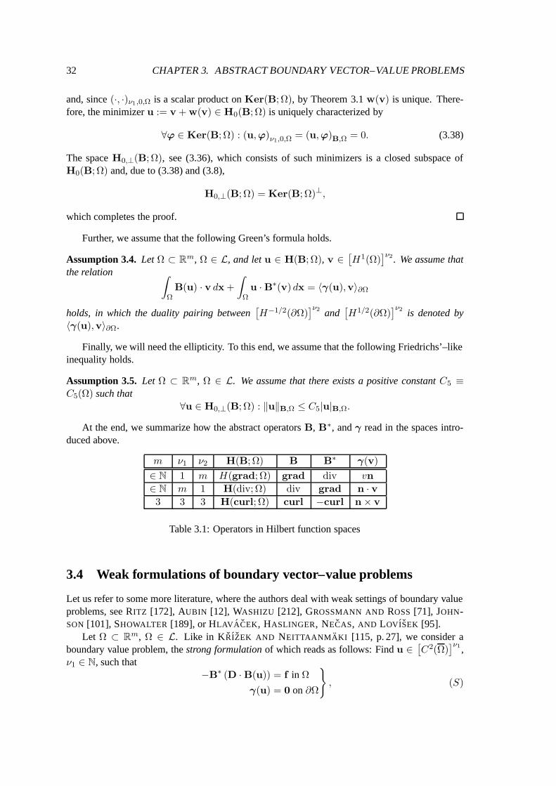
32 CHAPTER 3. ABSTRACT BOUNDARY VECTOR–VALUE PROBLEMS
and, since (·, ·)ν1 ,0,Ω is a scalar product on Ker(B; Ω), by Theorem 3.1 w(v) is unique. There-fore, the minimizer u := v + w(v) ∈ H0(B; Ω) is uniquely characterized by
∀ϕ ∈ Ker(B; Ω) : (u,ϕ)ν1,0,Ω = (u,ϕ)B,Ω = 0. (3.38)
The space H0,⊥(B; Ω), see (3.36), which consists of such minimizers is a closed subspace ofH0(B; Ω) and, due to (3.38) and (3.8),
H0,⊥(B; Ω) = Ker(B; Ω)⊥,
which completes the proof.
Further, we assume that the following Green’s formula holds.
Assumption 3.4. Let Ω ⊂ Rm, Ω ∈ L, and let u ∈ H(B; Ω), v ∈[H1(Ω)
]ν2 . We assume thatthe relation ∫
ΩB(u) · v dx +
∫
Ωu · B∗(v) dx = 〈γ(u),v〉∂Ω
holds, in which the duality pairing between[H−1/2(∂Ω)
]ν2 and[H1/2(∂Ω)
]ν2 is denoted by〈γ(u),v〉∂Ω .
Finally, we will need the ellipticity. To this end, we assume that the following Friedrichs’–likeinequality holds.
Assumption 3.5. Let Ω ⊂ Rm, Ω ∈ L. We assume that there exists a positive constant C5 ≡C5(Ω) such that
∀u ∈ H0,⊥(B; Ω) : ‖u‖B,Ω ≤ C5|u|B,Ω.
At the end, we summarize how the abstract operators B, B∗, and γ read in the spaces intro-duced above.
m ν1 ν2 H(B; Ω) B B∗ γ(v)
∈ N 1 m H(grad; Ω) grad div vn
∈ N m 1 H(div; Ω) div grad n · v3 3 3 H(curl; Ω) curl −curl n× v
Table 3.1: Operators in Hilbert function spaces
3.4 Weak formulations of boundary vector–value problems
Let us refer to some more literature, where the authors deal with weak settings of boundary valueproblems, see RITZ [172], AUBIN [12], WASHIZU [212], GROSSMANN AND ROSS [71], JOHN-SON [101], SHOWALTER [189], or HLAVACEK, HASLINGER, NECAS, AND LOVISEK [95].
Let Ω ⊂ Rm, Ω ∈ L. Like in KRIZEK AND NEITTAANMAKI [115, p. 27], we consider aboundary value problem, the strong formulation of which reads as follows: Find u ∈
[C2(Ω)
]ν1 ,ν1 ∈ N, such that
−B∗ (D · B(u)) = f in Ω
γ(u) = 0 on ∂Ω
, (S)
3.4. WEAK FORMULATIONS OF BOUNDARY VECTOR–VALUE PROBLEMS 33
where B, B∗, and γ are defined by Definition 3.2, and where D ∈[C1(Ω)
]ν2×ν2 , ν2 ∈ N, is auniformly positive definite real–valued matrix, i.e., there exists a constant C6 > 0 such that
∀x ∈ Ω∀v ∈ Rν2 : v · (D(x) · v) ≥ C6‖v‖2, (3.39)
and where f ∈[C(Ω)
]ν1 . The function u ∈[C2(Ω)
]ν1 is called the classical solution to (S).Now, we introduce a weak setting of (S), which will enable us to weaken the assumptions on
the differentiability of the data in (S) and to deal with problems of more practical purposes. Letus take into account the extensions of definitions of B, B∗, and γ from Section 3.3.6, as well asAssumptions 3.2–3.5 and Lemma 3.5 introduced there. We define the continuous bilinear forma : H(B; Ω) ×H(B; Ω) 7→ R and the continuous linear functional f : H(B; Ω) 7→ R by
a(v,u) :=
∫
ΩB(v) · (D ·B(u)) dx, u,v ∈ H(B; Ω), (3.40)
f(v) :=
∫
Ωf · v dx, v ∈ H(B; Ω), (3.41)
respectively, where f ∈[L2(Ω)
]ν1 , D := (di,j) is a matrix the entries of which di,j ∈ L∞(Ω),i, j = 1, . . . , ν2, and the condition (3.39) holds almost everywhere (a.e.) in Ω. A weak formulationof the problem (S) reads as follows:
Find u ∈ H0(B; Ω):
a(v,u) = f(v) ∀v ∈ H0(B; Ω)
. (3.42)
Just by applying Corollary 3.3, we can see that the classical solution u ∈[C2(Ω)
]ν1 of theproblem (S) is also a solution to (3.42). However, the problem (3.42) admits more general andphysically still reasonable data.
We can observe that if u ∈ H0(B; Ω) is a solution to (3.42), then for any p ∈ Ker(B; Ω)the function u + p is a solution, too. This indicates a Neumann–like problem. Therefore, werestrict our consideration onto the quotient space H0(B; Ω)/Ker(B; Ω), which is by Lemma 3.5isomorphically isometric to H0,⊥(B; Ω)), being a subspace of H0(B; Ω). In this case, we have tointroduce a compatibility condition on the right–hand side f
∀p ∈ Ker(B; Ω) :
∫
Ωf · p dx = 0. (3.43)
The correct weak formulation of (S) reads as follows:
Find u ∈ H0,⊥(B; Ω):
a(v,u) = f(v) ∀v ∈ H0,⊥(B; Ω)
, (W )
where f satisfies (3.43). It can be easily verified that a solution u to (W ) also solves the problem(3.42). On the other hand, the next theorem shows that (W ) has a unique solution, unlike theproblem (3.42).
Theorem 3.16. There exists exactly one solution u ∈ H0,⊥(B; Ω) to the problem (W ). Moreover,there exists a positive constant C7 such that
‖u‖B,Ω ≤ C7 ‖f‖ν1,0,Ω . (3.44)
34 CHAPTER 3. ABSTRACT BOUNDARY VECTOR–VALUE PROBLEMS
Proof. We will check the assumptions of Lemma 3.1 and the assertion then follows.Since H0,⊥(B; Ω) is a closed subspace of H0(B; Ω), it is also a Hilbert space equipped with
the scalar product (3.33). The form a is clearly bilinear. Concerning the matrix D, we denote
d := maxi,j
ess sup
x∈Ω|di,j(x)|
(3.45)
and, using (3.3) and (3.34), we prove the continuity of a as follows:
|a(v,u)| ≤ d
∣∣∣∣∫
ΩB(v) ·B(u) dx
∣∣∣∣ ≤ d ‖B(v)‖ν2 ,0,Ω ‖B(u)‖ν2 ,0,Ω ≤ d ‖v‖B,Ω ‖u‖B,Ω,
where u,v ∈ H(B; Ω), and where we used that D ∈ [L∞(Ω)]ν2×ν2 , (3.3), and (3.34), respec-tively. The H0,⊥(B; Ω)–ellipticity of a follows from
a(v,v) =
∫
ΩB(v) · (D · B(v)) dx ≥ C6
∫
Ω‖B(v)‖2 dx ≥ C6
C25
‖v‖2B,Ω, v ∈ H0,⊥(B; Ω),
(3.46)where (3.39) and Assumption 3.5 were used, respectively. Finally, f is obviously a linear func-tional on H(B; Ω) and it is continuous thereon, too, since
|f(v)| =
∣∣∣∣∫
Ωf · v dx
∣∣∣∣ ≤ ‖f‖ν1,0,Ω‖v‖ν1,0,Ω ≤ ‖f‖ν1,0,Ω‖v‖B,Ω, v ∈ H(B; Ω),
where we used (3.3) and (3.34), respectively. The assertion now follows from Lemma 3.1, wherethe H0,⊥(B; Ω)–ellipticity constant is
C7 :=C6
C25
.
3.4.1 A regularized formulation in H0(B)
In many cases, as in both 2d and 3d magnetostatics, we look for B(u) rather than for u, a solutionto (W ). Since there is the additional condition (3.38) in the definition of the space H0,⊥(B; Ω),it would be difficult to approximate the space by the finite element method. Therefore, we willintroduce a regularized weak formulation in the original space H0(B; Ω) such that its solutiontends towards the solution u ∈ H0(B; Ω) of the problem (W ), but in the seminorm | · |B,Ω only.
Let ε > 0 be a regularization parameter. We introduce the following bilinear form
aε(v,u) := a(v,u) + ε
∫
Ωv · u dx, u,v ∈ H(B; Ω), (3.47)
where a is given by (3.40). The regularized weak formulation reads as follows:
Find uε ∈ H0(B; Ω):
aε(v,uε) = f(v) ∀v ∈ H0(B; Ω)
, (Wε)
where f is given by (3.41) such that (3.43) holds.
Theorem 3.17. For each ε > 0 there exists a unique solution uε ∈ H0(B; Ω) to the problem(Wε). Moreover, there exists a positive constant C8(ε) such that
‖uε‖B,Ω ≤ C8(ε) ‖f‖ν1,0,Ω .
3.4. WEAK FORMULATIONS OF BOUNDARY VECTOR–VALUE PROBLEMS 35
Proof. The proof is fairly the same as the one of Theorem 3.16. The continuity of a is proven asfollows:
|aε(v,u)| ≤ d
∣∣∣∣∫
ΩB(v) ·B(u) dx
∣∣∣∣ + ε
∣∣∣∣∫
Ωv · u dx
∣∣∣∣ ≤ max d, ε ‖v‖B,Ω‖u‖B,Ω, (3.48)
where u,v ∈ H(B; Ω) and where d is given by (3.45). The H0(B; Ω)–ellipticity of aε followsfrom
aε(v,v) ≥ C6
∫
Ω‖B(v)‖2 dx + ε
∫
Ω|v|2 dx ≥ minC6, ε‖v‖2
B,Ω, v ∈ H(B; Ω),
where C6 is given by (3.39). Therefore, the H0(B; Ω)–ellipticity constant is
C8(ε) := minC6, ε. (3.49)
Theorem 3.18. The following holds:
B(uε) → B(u) in[L2(Ω)
]ν2 , as ε → 0+, (3.50)
where uε ∈ H0(B; Ω) are the solutions to (Wε) and u ∈ H0,⊥(B; Ω) is the solution to (W ).
Proof. Let ε > 0 be arbitrary. Using (3.39) and the definitions of (W ) and (Wε), we have
‖B(uε) −B(u)‖2ν2 ,0,Ω = |uε − u|2B,Ω =
∫
Ω‖B(uε) −B(u)‖2 dx ≤
≤ 1
C6
∫
ΩB(uε − u) · (D · B(uε − u)) dx =
1
C6a(uε − u,uε − u) ≤
≤ 1
C6aε(uε − u,uε − u)) =
1
C6(f(uε − u) − aε(uε − u,u)) =
=1
C6
(f(uε − u) − a(uε − u,u) − ε
∫
Ω(uε − u) · u dx
)
(3.51)Using the orthogonal decomposition (3.37), there exists uε,⊥ ∈ H0,⊥(B; Ω) and there existsuε,0 ∈ Ker(B; Ω) such that
uε = uε,⊥ + uε,0.
Using the latter, the condition (3.43), (3.38) and (3.25), the estimate (3.51) reads
‖B(uε) −B(u)‖2ν2 ,0,Ω = ‖B(uε,⊥) −B(u)‖2
ν2 ,0,Ω ≤
≤ 1
C6
(f(uε,⊥ − u) − a(uε,⊥ − u,u) − ε
∫
Ω(uε,⊥ − u) · u dx
)≤
≤ ε
C6
∣∣∣∣∫
Ω(uε,⊥ − u) · u dx
∣∣∣∣ ≤ε
C6‖uε,⊥ − u‖B,Ω‖u‖ν1,0,Ω.
Now we use Assumption 3.5
‖B(uε) −B(u)‖2ν2 ,0,Ω = |uε,⊥ − u|2B,Ω ≤ ε
C5
C6|uε,⊥ − u|B,Ω‖u‖ν1,0,Ω.
After dividing the latter by |uε,⊥ − u|B,Ω, the statement follows.
36 CHAPTER 3. ABSTRACT BOUNDARY VECTOR–VALUE PROBLEMS
3.4.2 A weak formulation of three–dimensional linear magnetostatics
Here we apply the results of the previous sections to the strong formulation (2.5).Let Ω ⊂ R3, Ω ∈ L. Taking a look into Table 3.1, at (S), and (2.5), we specify the symbols
B := curl, B∗ := −curl, and γ(v) := n× v|∂Ω,
where n := (n1, n2, n3) denotes the outer unit normal to ∂Ω. Due to (2.5), we determine thesymbols
D :=1
µ, f := J,
where µ ∈ L∞(Ω), µ > 0 a.e. in Ω, J ∈[L2(Ω)
]3. The condition (3.39) is now equivalent to
∃µ1 > 0 : µ(x) ≤ µ1 a.e. in Ω (3.52)
in such a way that
C6 :=1
µ1.
Since Ker(curl; Ω) is equal to the space H0,0(curl; Ω) defined by (3.29) the condition (3.43)reads as follows:
∀p ∈ H10 (Ω) :
∫
ΩJ · grad(p) dx = 0.
Finally, we specify the terms in (W ). As we have seen in Section 3.3.4, the quotient spaceH0(curl; Ω)/Ker(curl; Ω) is isomorphically isometric to the space H0,⊥(curl; Ω), which wasdefined by (3.30). The bilinear form (3.40) and the linear form (3.41) are, respectively, determinedby
a(v,u) :=
∫
Ωcurl(v) ·
(1
µcurl(u)
)dx, u,v ∈ H(curl; Ω),
and by
f(v) :=
∫
ΩJ · v dx, v ∈ H(curl; Ω).
We have specified all the assumptions on the abstract weak formulation (W ) introduced in Sec-tion 3.4. Therefore, Theorem 3.16 holds with the H0,⊥(curl; Ω)–ellipticity constant
C7 :=1
µ0C24
,
where C4 is given by Theorem 3.13. In case of the formulation (Wε), we only recall the regularizedbilinear form
aε(v,u) :=
∫
Ωcurl(v) ·
(1
µcurl(u)
)dx + ε
∫
Ωv · u dx, u,v ∈ H(curl; Ω),
whose ellipticity constant is given by (3.49).
3.4. WEAK FORMULATIONS OF BOUNDARY VECTOR–VALUE PROBLEMS 37
3.4.3 A weak formulation of two–dimensional linear magnetostatics
Now we apply the results of Section 3.4 to the strong formulation (2.6).Let Ω ⊂ R2, Ω ∈ L. We specify the symbols
B := grad, B∗ := −div, and γ(v) := v|∂Ωn,
where n := (n1, n2) denotes the outer unit normal to ∂Ω. Due to (2.6), we determine the symbols
D :=1
µ, f := J, (3.53)
where µ ∈ L∞(Ω), µ > 0 a.e. in Ω, J ∈ L2(Ω). We again replace the condition (3.39) by (3.52).Since Ker(grad; Ω) defined by (3.28) is equal to the zero space 0, the condition (3.43) alwaysholds and does not need to be introduced in this case. Finally, we specify the terms in (W ). Aswe have seen in Section 3.3.3, the quotient space H0(grad; Ω)/0 is equal to the space H1
0 (Ω).The bilinear form (3.40) and the linear functional (3.41) are, respectively, determined by
a(v, u) :=
∫
Ωgrad(v) ·
(1
µgrad(u)
)dx, u, v ∈ H1(Ω),
and by
f(v) :=
∫
ΩJv dx, v ∈ H1(Ω).
Now, Theorem 3.16 holds with the H10 (Ω)–ellipticity constant
C7 :=1
µ0C23
,
where C3 is given by Theorem 3.9. In this case, we do not need to introduce the regularizedproblem (Wε), since all the spaces are equal
H0,⊥(grad; Ω) = H0(grad; Ω) = H10 (Ω).

38 CHAPTER 3. ABSTRACT BOUNDARY VECTOR–VALUE PROBLEMS
Chapter 4
Finite element method
In this chapter, we will recall the basic techniques of the finite element method. First, we willpresent the ideas and concept of the method. Then, we will deal with algorithmic issues. Further,approximation properties will be proved. At the end, we will describe the finite elements usedfor the linear magnetostatics, namely Lagrange nodal elements on triangles and Nedelec edgeelements on tetrahedra. We refer to KRIZEK AND NEITTAANMAKI [115, Chapter 4] for a detaileddescription of the method.
The large popularity of the method can be documented by the following unsorted list of lit-erature: GIRAULT AND RAVIART [67], BRAESS [27], BOSSAVIT [26], STRANG AND FIX [200],CIARLET [45], ZLAMAL [219], RAVIART AND THOMAS [167], HIPTMAIR [91, 93], ZIENKIE-WICZ [217], ZIENKIEWICZ AND TAYLOR [218], HASLINGER, MIETTINEN, AND PANAGIOTOP-ULOS [84], BREZZI AND FORTIN [33], HUGHES [98], JUNG AND LANGER [103], BRENNER
AND SCOTT [32], GROSSMANN AND ROSS [71], JOHNSON [101], KIKUCHI [108], ODEN AND
REDDY [150], SCHWAB [187], SZABO AND BABUSKA [205], BABUSKA AND AZIZ [14, 15],GLOWINSKI [68], KRIZEK AND NEITTAANMAKI [114, 115], KRIZEK [113], NEITTAANMAKI
AND SARANEN [147, 146], SILVESTER AND FERRARI [192], HACKBUSCH AND SAUTER [79,80].
4.1 The concept of the method
We consider the regularized weak formulation (Wε) of the abstract elliptic linear boundary vector–value problem (S), which was introduced in Section 3.4.1. The aim of this chapter is to developa method which approximates the continuous regularized solution uε of the problem (Wε) by asequence of some discretized solutions uh
ε , where h > 0 stands for a discretization parameter.
4.1.1 Galerkin approximation
Let Vh ⊂ H0(B; Ω) be a closed subspace. We introduce approximations of the bilinear form (3.47)and of the linear functional (3.41), respectively, by
ahε (v,w) :=
∫
ΩB(v) ·
(Dh · B(w)
)dx + ε
∫
Ωv · w dx, v,w ∈ H(B; Ω), (4.1)
fh(v) :=
∫
Ωfh · v dx, v ∈ H(B; Ω), (4.2)
39
40 CHAPTER 4. FINITE ELEMENT METHOD
where fh ∈(L2(Ω)
)ν1 is such that
∀h > 0 ∀p ∈ Ker(B; Ω) :
∫
Ωfh · p dx = 0,
and where Dh :=(dh
i,j
)ν2
i,j=1is a matrix the entries of which dh
i,j ∈ L∞(Ω) and such that
∀h > 0 : ess supx∈Ω
∣∣∣dhi,j(x)
∣∣∣ ≤ ess supx∈Ω
|di,j(x)| , i, j = 1, . . . , ν2. (4.3)
Both fh and Dh are assumed to be piecewise constant. Moreover, we suppose that
∀h > 0 ∀v ∈ Rν2 : v ·(Dh(x) · v
)≥ C6‖v‖2 a.e. in Ω, (4.4)
where C6 > 0 is given by (3.39). We consider the following problem
Find uhε ∈ Vh:
ahε
(vh,uh
ε
)= fh
(vh)
∀vh ∈ Vh
, (W h
ε )
which is called the Galerkin approximation to the problem (Wε).
Theorem 4.1. For each ε > 0 and h > 0 there exists a unique solution uhε ∈ Vh to the problem
(W hε ). Moreover, there exists a positive constant C8(ε) such that
∀h > 0 : ‖uhε‖B,Ω ≤ C8(ε)
∥∥∥fh∥∥∥
ν1,0,Ω.
Proof. The proof is fairly the same as the one of Theorem 3.17.Let ε > 0 and h > 0 be arbitrary. By definition, Vh is a closed subspace of H0(B; Ω),
therefore, it is also a Hilbert space. The form ahε is obviously bilinear and fh is a linear functional
on Vh. We have the continuity of ahε
∣∣∣ahε (v,w)
∣∣∣ ≤ maxdh, ε ‖v‖B,Ω ‖w‖B,Ω , v,w ∈ H(B; Ω),
where
dh := maxi,j
ess sup
x∈Ω
∣∣∣dhi,j(x)
∣∣∣
.
Due to (4.4), we have the Vh–ellipticity of ahε
ahε (v,v) ≥ minC6, ε ‖v‖2
B,Ω , v ∈ H(B; Ω),
independently of h. Finally, the continuity of f h follows from
fh(v) ≤∥∥∥fh∥∥∥
ν1,0,Ω‖v‖B,Ω , v ∈ H(B; Ω).
Therefore, the assertion follows with the Vh–ellipticity constant
C8(ε) := minC6, ε. (4.5)
4.1. THE CONCEPT OF THE METHOD 41
The following lemma, cf. BRAESS [27], CIARLET [45], or STRANG AND FIX [200], saysthat we can study the approximation properties of uh
ε via the approximation of H0(B; Ω) by itssubspaces Vh and via the approximation properties of the forms ah
ε and fh.
Lemma 4.1. (1st Strang’s lemma) Let ε > 0 and h > 0 be a regularization and discretizationparameter, respectively. Then there exists a positive constant C9(ε), independent of h, such that
∀vh ∈ Vh :∥∥∥uε − uh
ε
∥∥∥B,Ω
≤ C9(ε)
∥∥∥uε − vh∥∥∥B,Ω
+
+
∣∣aε
(vh,uh
ε − vh)− ah
ε
(vh,uh
ε − vh)∣∣
‖uhε − vh‖B,Ω
+
+
∣∣f(uh
ε − vh)− fh
(uh
ε − vh)∣∣
‖uhε − vh‖B,Ω
,
where uε ∈ H0(B; Ω) is a solution to (Wε) and uhε ∈ Vh are solutions to (W h
ε ).
Proof. Let h > 0 and vh ∈ Vh be arbitrary. By the triangle inequality,∥∥∥uε − uh
ε
∥∥∥B,Ω
≤∥∥∥uε − vh
∥∥∥B,Ω
+∥∥∥uh
ε − vh∥∥∥B,Ω
. (4.6)
To make the proof more readable, we introduce the symbol
whε := uh
ε − vh. (4.7)
Now, we use the Vh–ellipticity of aε, the bilinearity of aε, ahε , and the definitions of prob-
lems (Wε), (W hε ), respectively, and we get
C8(ε)∥∥∥wh
ε
∥∥∥2
B,Ω≤ ah
ε
(wh
ε ,whε
)= aε
(wh
ε ,uε − vh)− aε
(wh
ε ,uε − vh)
+ ahε
(wh
ε ,whε
)=
= aε
(wh
ε ,uε − vh)
+(aε
(wh
ε ,vh)− ah
ε
(wh
ε ,vh))
+
+(ah
ε
(wh
ε ,uhε
)− aε
(wh
ε ,uε
))=
= aε
(wh
ε ,uε − vh)
+(aε
(wh
ε ,vh)− ah
ε
(wh
ε ,vh))
+
+(fh(wh
ε
)− f
(wh
ε
)).
Dividing the latter by ‖whε ‖B,Ω and using (3.48) yield
C8(ε)∥∥∥wh
ε
∥∥∥B,Ω
≤ maxd, ε∥∥∥uε − vh
∥∥∥B,Ω
+
∣∣aε
(vh,wh
ε
)− ah
ε
(vh,wh
ε
)∣∣‖wh
ε‖B,Ω
+
+
∣∣f(wh
ε
)− fh
(wh
ε
)∣∣‖wh
ε‖B,Ω
.
(4.8)
Combining (4.5), (4.6), (4.7), and (4.8), the assertion is proved, where the constant is as follows:
C9(ε) := max
1 +
maxd, εminC6, ε
,1
minC6, ε
.
42 CHAPTER 4. FINITE ELEMENT METHOD
4.1.2 Finite element method
Let Vh be of a finite dimension. Having a base v1, . . . ,vn of the space Vh, the problem (W hε )
is equivalent to the following system of linear equations
Anε · un
ε = f n, (4.9)
where the matrix Anε ∈ Rn×n and the right–hand side vector f n ∈ Rn are as follows:
Anε :=
(ah
ε (vi,vj))n
i,j=1, f n :=
(fh(vi)
)n
i=1, (4.10)
respectively, and the solution vector unε :=
(un
ε,1, . . . , unε,n
)∈ Rn corresponds to the approximate
solution uhε in the following way
uhε =
n∑
i=1
unε,ivi.
The finite element method is a special case of the Galerkin method. The base v1, . . . ,vnof the space Vh is chosen such that the matrix An
ε is sparse. In this case the system (4.9) can besolved much faster and the matrix An
ε takes less computer memory. The finite element method isdetermined as follows:
• The domain Ω ⊂ Rm is decomposed into smaller convex subdomains, e.g., line segmentsfor m = 1, triangles for m = 2, or tetrahedra for m = 3.
• The base v1, . . . ,vn is chosen as simple functions, e.g., polynomials. The space Vh iscalled the space of finite elements.
• The basis functions v1, . . . ,vn have small supports, which make the matrix Anε to be sparse.
4.1.3 Discretization of the domain
We will employ polyhedral elements. To this end, we have to replace the original domain Ω bya polyhedral subdomain Ωh. We subdivide Ωh into a finite number of polyhedral subdomainsK1, . . . ,Kn
Ωh, nΩh ∈ N, i.e., into open and connected polyhedral subsets of Ωh such that the
following assumptions are satisfied:
• Ωh =n
Ωh⋃i=1
Ki ,
• Ki 6= ∅ for each i = 1, . . . , nΩh ,
• Ki 6= Kj ⇒ Ki ∩ Kj = ∅ for each i, j = 1, . . . , nΩh ,
• any face of any Ki is either a subset of the boundary ∂Ωh or a face of another element Kj ,where i, j = 1, . . . , nΩh ,
• each Ki has exactly m + 1 faces.
The last assumption means that in the cases of m = 1, m = 2, and m = 3 we deal with linesegments, triangles, and tetrahedra, respectively. This assumption will provide us to introduce areference element.
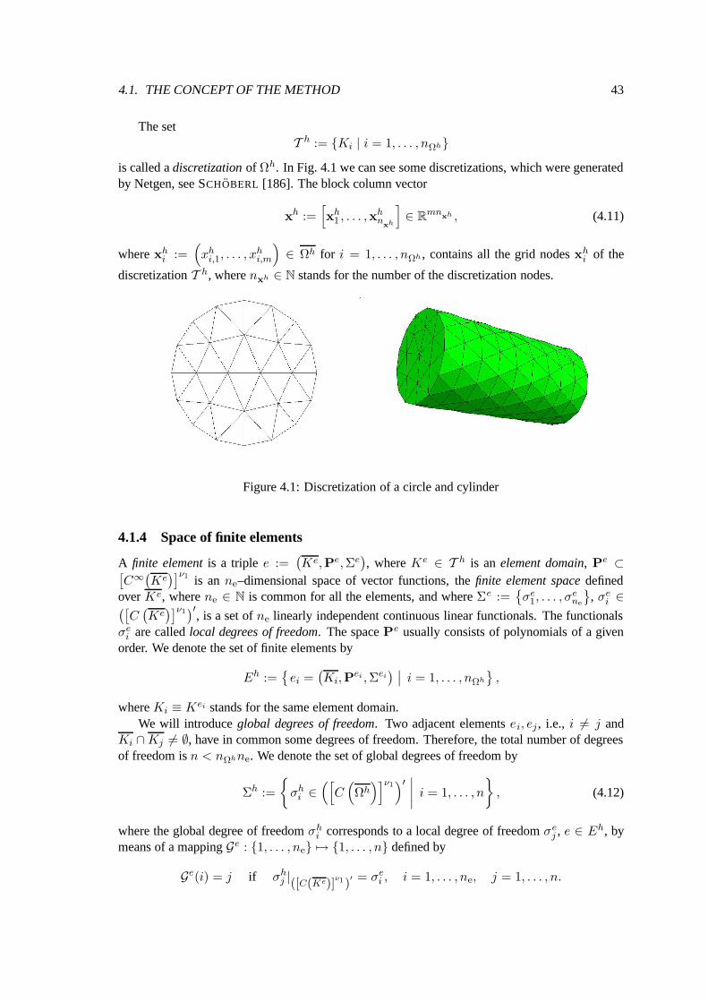
4.1. THE CONCEPT OF THE METHOD 43
The setT h := Ki | i = 1, . . . , nΩh
is called a discretization of Ωh. In Fig. 4.1 we can see some discretizations, which were generatedby Netgen, see SCHOBERL [186]. The block column vector
xh :=[xh
1 , . . . ,xhnx
h
]∈ Rmn
xh , (4.11)
where xhi :=
(xh
i,1, . . . , xhi,m
)∈ Ωh for i = 1, . . . , nΩh , contains all the grid nodes xh
i of the
discretization T h, where nxh ∈ N stands for the number of the discretization nodes.
Figure 4.1: Discretization of a circle and cylinder
4.1.4 Space of finite elements
A finite element is a triple e :=(Ke,Pe,Σe
), where Ke ∈ T h is an element domain, Pe ⊂[
C∞(Ke)]ν1 is an ne–dimensional space of vector functions, the finite element space defined
over Ke, where ne ∈ N is common for all the elements, and where Σe :=σe
1, . . . , σene
, σe
i ∈([C(Ke)]ν1
)′, is a set of ne linearly independent continuous linear functionals. The functionals
σei are called local degrees of freedom. The space Pe usually consists of polynomials of a given
order. We denote the set of finite elements by
Eh :=
ei =(Ki,P
ei ,Σei) ∣∣ i = 1, . . . , nΩh
,
where Ki ≡ Kei stands for the same element domain.We will introduce global degrees of freedom. Two adjacent elements ei, ej , i.e., i 6= j and
Ki ∩ Kj 6= ∅, have in common some degrees of freedom. Therefore, the total number of degreesof freedom is n < nΩhne. We denote the set of global degrees of freedom by
Σh :=
σh
i ∈([
C(Ωh)]ν1
)′ ∣∣∣∣ i = 1, . . . , n
, (4.12)
where the global degree of freedom σhi corresponds to a local degree of freedom σe
j , e ∈ Eh, bymeans of a mapping Ge : 1, . . . , ne 7→ 1, . . . , n defined by
Ge(i) = j if σhj |([C(Ke)]
ν1)′ = σe
i , i = 1, . . . , ne, j = 1, . . . , n.
44 CHAPTER 4. FINITE ELEMENT METHOD
Since dim(Pe) = ne, ne ∈ N, and σe1, . . . , σ
ene
∈ Σe are linearly independent, then thereexists a basis
ξe
1, . . . , ξene
⊂ Pe such that
σei
(ξe
j
)= δi,j , i, j = 1, . . . , ne, where δi,j :=
1 , i = j
0 , i 6= j.
These base functions are called shape functions. In the same virtue, we introduce global shapefunctions ξh
1 , . . . , ξhn : Ωh 7→ Rν1 such that
σhi
(ξh
j
)= δi,j, i, j = 1, . . . , n. (4.13)
The global shape functions correspond to the local ones as follows:
ξhGe(i)|Ke = ξe
i , e ∈ Eh, i = 1, . . . , ne.
The global shape functions form a basis for the following space
Ph :=
vh =
n∑
i=1
viξhi
∣∣∣∣∣ v1, . . . , vn ∈ R
. (4.14)
Hence, the space Ph consists of such functions that are elementwise in Pe, i.e.,
∀vh ∈ Ph ∀e ∈ Eh : vh|Ke ∈ Pe
We need Ph to be a subspace of H(B; Ωh
). This property is called the conformity of the finite
elements. The following lemma gives a sufficient condition on the conformity.
Lemma 4.2. Let vh ∈ Ph. Then vh ∈ H(B; Ωh
)if for any two adjacent elements ei, ej ∈ Eh,
i 6= j, with a common face fi,j := Ki ∩ Kj , the trace γ is continuous over fi,j , i.e.,
γKi
(vh|Ki
)|fi,j
= −γKj
(vh|Kj
)|fi,j
, (4.15)
where γ is given by (3.23). Note that the minus sign appeared, since the outer unit normal vectorson fi,j satisfy nKi
= −nKj.
Proof. Let vh ∈ Ph and let (4.15) holds. Clearly vh ∈[L2(Ωh)]ν1 . We will prove that vh ∈
H(B; Ωh
)by means of (3.32). We take zh ∈
[L2(Ωh)]ν2 such that
zh|Ki:= B
(vh|Ki
), i = 1, . . . , nΩh .
Let wh ∈[C∞
0
(Ωh)]ν2 be arbitrary. Then, Corollary 3.3 and (4.15) yield
∫
Ωh
vh ·B∗(wh)
dx =∑
Ki∈T h
∫
Ki
vh ·B∗(wh)
dx =
=∑
Ki∈T h
(−∫
Ki
zh · wh dx +
∫
∂Ki
γKi
(vh)·wh ds
)=
= −∫
Ωh
zh · wh dx +∑
fi,j
(∫
fi,j
γKi
(vh)·wh ds +
∫
fi,j
γKj
(vh)·wh ds
)=
= −∫
Ωh
zh · wh dx,
which completes the proof.
4.1. THE CONCEPT OF THE METHOD 45
The next assumption ensures the conformity of the finite elements, i.e., Ph ⊂ H(B; Ωh
). We
refer to HIPTMAIR [92] for a unified way of the design of conforming finite elements.
Assumption 4.1. Let e ∈ Eh be an element and let f ⊂ ∂Ke denote a face. We assume thatthe degrees of freedom connected to the face f are exactly the ones which determine the traceγKe(ve) |f , where ve ∈ Pe.
Further, we introduce the set of indices of those degrees of freedom which determine the traceγΩh . Due to (4.14), we can write an arbitrary vh ∈ Ph as
vh =n∑
i=1
vhi ξ
hi ,
where vhi ∈ R for i = 1, . . . , n and where ξh
i denote the global shape functions. Then,
γΩh
(vh)
=n∑
i=1
vhi γΩh
(ξh
i
).
Therefore, the trace is determined by the following set of indices
Ih0 :=
i ∈ 1, . . . , n
∣∣∣ γΩh
(ξh
i
)6= 0
. (4.16)
Then, the finite element space Vh ≡ H0
(B; Ωh
)h ⊂ H0
(B; Ωh
)is defined by
H0
(B; Ωh
)h:=
vh ∈ Ph∣∣∣ ∀i ∈ Ih
0 : σhi
(vh)
= 0
. (4.17)
4.1.5 Finite element discretization of the weak formulation
Let Ω ⊂ Rm, Ω ∈ L. We rewrite the problem (Wε) as follows:
Find uε(Ω) ∈ H0(B; Ω):
aε(v,uε(Ω)) = f(v) ∀v ∈ H0(B; Ω)
. (Wε(Ω))
As long as Ω ∈ L, the existence of the unique solution uε(Ω) to (Wε(Ω)) is given by Theo-rem 3.17.
Further, let h > 0 be a discretization parameter and let Ωh ⊂ Ω be a nonempty polyhedralsubdomain. Then, Ωh ∈ L. Let T h be a discretization of Ωh and let Eh be the corresponding setof finite elements. Concerning the bilinear form ah
ε and the linear functional fh given by (4.1) and(4.2), respectively, we assume that for each e ∈ Eh there exist a constant matrix De ∈ Rν2×ν2
and vector f e ∈ Rν1 such that
∀x ∈ Ke : Dh(x) = De and fh(x) = f e. (4.18)
The Galerkin approximation of the problem (Wε(Ωh)) reads as follows:
Find uhε
(Ωh)∈ H0
(B; Ωh
)h:
ahε
(vh,uh
ε
(Ωh))
= fh(vh)
∀vh ∈ H0
(B; Ωh
)h
, (W hε (Ωh))
where ahε , fh, and H0
(B; Ωh
)hare respectively defined by (4.1), (4.2), and by (4.17). The exis-
tence and uniqueness of the solution uhε
(Ωh)
to (W hε ) follows from Theorem 4.1.
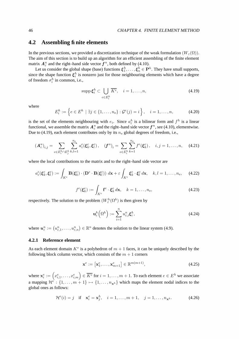
46 CHAPTER 4. FINITE ELEMENT METHOD
4.2 Assembling finite elements
In the previous sections, we provided a discretization technique of the weak formulation (Wε(Ω)).The aim of this section is to build up an algorithm for an efficient assembling of the finite elementmatrix An
ε and the right–hand side vector f n, both defined by (4.10).Let us consider the global shape (base) functions ξh
1 , . . . , ξhn ∈ Ph. They have small supports,
since the shape function ξhi is nonzero just for those neighbouring elements which have a degree
of freedom σhi in common, i.e.,
supp ξhi ⊂
⋃
e∈Ehi
Ke, i = 1, . . . , n, (4.19)
whereEh
i :=
e ∈ Eh | ∃j ∈ 1, . . . , ne : Ge(j) = i
, i = 1, . . . , n, (4.20)
is the set of the elements neighbouring with ei. Since ahε is a bilinear form and fh is a linear
functional, we assemble the matrix Anε and the right–hand side vector f n, see (4.10), elementwise.
Due to (4.19), each element contributes only by its ne global degrees of freedom, i.e.,
(Anε )i,j =
∑
e∈Ehi ∩Eh
j
ne∑
k,l=1
aeε(ξ
ek, ξ
el ) , (f n)i =
∑
e∈Ehi
ne∑
k=1
f e(ξek) , i, j = 1, . . . , n, (4.21)
where the local contributions to the matrix and to the right–hand side vector are
aeε(ξ
ek, ξ
el ) :=
∫
Ke
B(ξek) · (De · B(ξe
l )) dx + ε
∫
Ke
ξek · ξe
l dx, k, l = 1, . . . , ne, (4.22)
f e(ξek) :=
∫
Ke
f e · ξek dx, k = 1, . . . , ne, (4.23)
respectively. The solution to the problem (W hε (Ωh) is then given by
uhε
(Ωh)
:=n∑
i=1
unε,iξ
hi , (4.24)
where unε :=
(un
ε,1, . . . , unε,n
)∈ Rn denotes the solution to the linear system (4.9).
4.2.1 Reference element
As each element domain Ke is a polyhedron of m + 1 faces, it can be uniquely described by thefollowing block column vector, which consists of the m + 1 corners
xe :=[xe
1, . . . ,xem+1
]∈ Rm(m+1), (4.25)
where xei :=
(xe
i,1, . . . , xei,m
)∈ Ke for i = 1, . . . ,m + 1. To each element e ∈ Eh we associate
a mapping He : 1, . . . ,m + 1 7→ 1, . . . , nxh which maps the element nodal indices to theglobal ones as follows:
He(i) = j if xei = xh
j , i = 1, . . . ,m + 1, j = 1, . . . , nxh . (4.26)
4.2. ASSEMBLING FINITE ELEMENTS 47
We further introduce a reference element r :=(Kr,Pr,Σr
)such that the polyhedral domain Kr
is determined by the following block column vector consisting of the reference corners
xr :=[xr
1, . . . , xrm+1
]∈ Rm(m+1),
where xri :=
(xr
i,1, . . . , xri,m
)∈ Kr, i = 1, . . . ,m + 1, and where dim(Pr) = dim(Pe) = ne.
To each element e ∈ Eh, we associate a one–to–one linear mapping Re : Kr 7→ Ke defined by
x := Re(x) := Re · x + re, x ∈ Ke, x ∈ Kr, (4.27)
where Re ∈ Rm×m is a nonsingular matrix and re ∈ Rm is a vector both of which are uniquelydetermined by xe as follows:
Re · xri + re = xe
i , i = 1, . . . ,m + 1. (4.28)
Obviously, both Re and re are continuously differentiable with respect to each coordinate of thecorners xe.
PSfrag replacements
00
1
1 x1
x2
Kr
Re
x1
x2
Ke
Figure 4.2: A transformation between the reference and an element domainPSfrag replacements
0
1
1
1
x1
x2
v
v
Kr
Se
x1
x2
v
Ke
Se(v)
Figure 4.3: A transformation between the reference and an element shape function
Further, let us denote by ξr1, . . . , ξ
rne
the shape functions acting on the reference element r,i.e.,
σri
(ξr
j
)= δi,j , i, j = 1, . . . , ne.
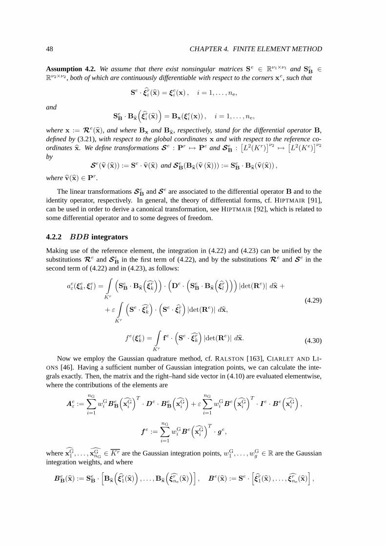
48 CHAPTER 4. FINITE ELEMENT METHOD
Assumption 4.2. We assume that there exist nonsingular matrices Se ∈ Rν1×ν1 and SeB ∈
Rν2×ν2 , both of which are continuously differentiable with respect to the corners xe, such that
Se · ξri (x) = ξe
i (x) , i = 1, . . . , ne,
andSe
B ·Bbx
(ξr
i (x))
= Bx(ξei (x)) , i = 1, . . . , ne,
where x := Re(x), and where Bx and Bbx, respectively, stand for the differential operator B,defined by (3.21), with respect to the global coordinates x and with respect to the reference co-ordinates x. We define transformations Se : Pr 7→ Pe and Se
B :[L2(Kr)
]ν2 7→[L2(Ke)
]ν2
bySe(v (x)) := Se · v(x) and Se
B(Bbx(v (x))) := SeB · Bbx(v(x)) ,
where v(x) ∈ Pr.
The linear transformations SeB and Se are associated to the differential operator B and to the
identity operator, respectively. In general, the theory of differential forms, cf. HIPTMAIR [91],can be used in order to derive a canonical transformation, see HIPTMAIR [92], which is related tosome differential operator and to some degrees of freedom.
4.2.2 BDB integrators
Making use of the reference element, the integration in (4.22) and (4.23) can be unified by thesubstitutions Re and Se
B in the first term of (4.22), and by the substitutions Re and Se in thesecond term of (4.22) and in (4.23), as follows:
aeε(ξ
ek, ξ
el ) =
∫
Kr
(Se
B · Bbx
(ξr
k
))·(De ·
(Se
B ·Bbx
(ξr
l
)))|det(Re)| dx +
+ ε
∫
Kr
(Se · ξr
k
)·(Se · ξr
l
)|det(Re)| dx,
(4.29)
f e(ξek) =
∫
Kr
f e ·(Se · ξr
k
)|det(Re)| dx. (4.30)
Now we employ the Gaussian quadrature method, cf. RALSTON [163], CIARLET AND LI-ONS [46]. Having a sufficient number of Gaussian integration points, we can calculate the inte-grals exactly. Then, the matrix and the right–hand side vector in (4.10) are evaluated elementwise,where the contributions of the elements are
Aeε :=
nG∑
i=1
wGi Be
B
(xG
i
)T·De · Be
B
(xG
i
)+ ε
nG∑
i=1
wGi Be
(xG
i
)T· I e ·Be
(xG
i
),
f e :=
nG∑
i=1
wGi Be
(xG
i
)T· g e,
where xG1 , . . . , xG
nG∈ Kr are the Gaussian integration points, wG
1 , . . . , wGg ∈ R are the Gaussian
integration weights, and where
BeB(x) := Se
B ·[Bbx
(ξr
1(x))
, . . . ,Bbx
(ξr
ne(x))]
, B e(x) := Se ·[ξr
1(x) , . . . , ξrne
(x)],
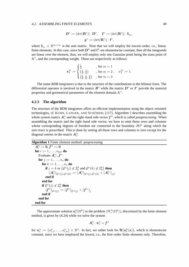
4.2. ASSEMBLING FINITE ELEMENTS 49
De := |det(Re)| ·De, I e := |det(Re)| · Ine,
g e := |det(Re)| · f e,
where Ine∈ Rne×ne is the unit matrix. Note that we will employ the lowest–order, i.e., linear,
finite elements. In this case, since both Dh and fh are elementwise constant, then all the integrandsare linear over the element, thus, we will employ only one Gaussian point being the mass point ofKr, and the corresponding weight. These are respectively as follows:
xG1 :=
12 , for m = 1(13 , 1
3
), for m = 2(
16 , 1
6 , 16
), for m = 3
, wG1 := 1.
The name BDB integrators is due to the structure of the contributions to the bilinear form. Thedifferential operator is involved in the matrix B e while the matrix De or I e provide the materialproperties and geometrical parameters of the element domain K e.
4.2.3 The algorithm
The structure of the BDB integrators offers an efficient implementation using the object–orientedtechnologies, cf. KUHN, LANGER, AND SCHOBERL [117]. Algorithm 1 describes assembling thewhole system matrix An
ε and the right–hand side vector f n, which is called postprocessing. Whenassembling the matrix and the right–hand side vector, we have to omit those rows and columnswhose corresponding degrees of freedom are connected to the boundary ∂Ωh along which thezero trace is prescribed. This is done by setting all those rows and columns to zero except for thediagonal entries in the matrix An
ε .
Algorithm 1 Finite element method: preprocessingAn
ε := 0, f n := 0
for i := 1, . . . , nΩh doEvaluate Aei
ε , f ei
for j := 1, . . . , ne dofor k := 1, . . . , ne do
if j = k or(Gei(j) 6∈ Ih
0 and Gei(k) 6∈ Ih0
)then
(Anε )Gei(j),Gei(k) := (An
ε )Gei(j),Gei(k) + (Aeiε )j,k
end ifend forif Gei(j) 6∈ Ih
0 then(f n)Gei(j) := (f n)Gei(j) + (f ei)j
end ifend for
end for
The approximate solution uhε
(Ωh)
to the problem (W hε (Ωh)), discretized by the finite element
method, is given by (4.24) while we solve the system
Anε · un
ε = f n
for unε :=
(un
ε,1, . . . , unε,n
)∈ Rn. In fact, we rather look for B
(uh
ε (x)), which is elementwise
constant, since we have employed the lowest, i.e., the first–order finite elements only. Therefore,

50 CHAPTER 4. FINITE ELEMENT METHOD
we can describe B(uh
ε (x))
by the block column vector
Bnε :=
[Bn,e1
ε , . . . ,Bn,en
Ωh
ε
]∈ Rν2n
Ωh
such that
B(uh
ε (x))|Ki
= Bn,eiε ,
where
Bn,eiε :=
ne∑
j=1
unε,Gei(j)S
ei
B ·Bbx
(ξr
j(x))∈ Rν2 for i = 1, . . . , nΩh .
This procedure which assembles the vector Bnε is called postprocessing and it is depicted in Al-
gorithm 2.
Algorithm 2 Finite element method: postprocessingGiven un
ε
Bnε := 0
for i := 1, . . . , nΩh doBn,ei
ε := 0
for j := 1, . . . , ne doEvaluate Bn,ei
ε := Bn,eiε + un
ε,Gei(j)Sei
B · Bbx
(ξr
j(x))
end fork := ν2(i − 1)for j := 1, . . . , ν2 do
[Bnε ]k+j := [Bn,ei
ε ]jend for
end for
4.3 Approximation properties
Now, we specify the meaning of the discretization parameter h in the formulation (W hε (Ωh)).
To each element domain Ke we associate an element discretization parameter he which is themaximum edge size of Ke, i.e., the length of the line segment, the maximum side of the triangle,or the maximum edge of the tetrahedron in the cases of m = 1, m = 2, or m = 3, respectively.The (global) discretization parameter h is defined by
h := maxe∈Eh
he. (4.31)
Convention 4.1. In what follows, we will assume that there exists h > 0, being, e.g., the minimumdiameter of a sphere (or circle) containing Ω, such that any considered discretization parameterh fulfills
h ≤ h. (4.32)
The aim of this section is to prove a convergence, in some sense, of the approximate finiteelement solutions uh
ε
(Ωh)
to the true solution uε(Ω).

4.3. APPROXIMATION PROPERTIES 51
4.3.1 Approximation of the domain by polyhedra
We employ polyhedral elements. Therefore, we have to deal with an approximation of the originaldomain Ω by polyhedra and with a convergence of solutions over these polyhedra.
We introduce an extension operator. Let h > 0, ν ∈ N, and let Ωh ⊂ Ω be a nonemptypolyhedral subdomain. We define a linear extension operator Xh
ν :[L2(Ωh)]ν 7→
[L2(Ω)
]νby
Xhν(v(x)) :=
v(x) , x ∈ Ωh
0 , x ∈ Ω \ Ωh, v(x) ∈
[L2(Ωh)]ν
. (4.33)
Lemma 4.3. Let Ω ⊂ Rm, Ω ∈ L be a domain, let Ωh ⊂ Ω be its nonempty polyhedral sub-
domain, and let vh ∈ H0
(B; Ωh
)h, where H0
(B; Ωh
)his defined by (4.17). Then Xh
ν1
(vh)∈
H0(B; Ω) and the space
X0
(B; Ω;Ωh
)h:=
Xh
ν1
(vh)∈ H0(B; Ω)
∣∣∣∣ vh ∈ H0
(B; Ωh
)h
(4.34)
is a closed subspace of H0(B; Ω).
Proof. Let vh ∈ H0
(B; Ωh
)hbe arbitrary. We denote bh := Xh
ν2
(B(vh))
. Clearly, bh ∈[L2(Ω)
]ν2 . Let ϕ ∈ [C∞0 (Ω)]ν2 , then ϕ|Ωh ∈
[H1(Ωh)]ν2 . Now the definition (4.33), Assump-
tion 3.4, and γΩh
(vh)
= 0, which is the trace along ∂Ωh, yield
∫
Ωbh ·ϕ dx =
∫
Ωh
B(vh)·ϕ|Ωh dx = −
∫
Ωh
vh · B∗(ϕ|Ωh) dx +⟨γΩh
(vh)
,ϕ|Ωh
⟩∂Ωh
=
= −∫
ΩXh
ν1
(vh)· B∗(ϕ) dx.
The latter implies that bh = B(Xh
ν1
(vh))
and Xhν1
(vh)∈ H(B; Ω). Further, letψ ∈
[H1(Ω)
]ν2 ,then ψ|Ωh ∈
[H1(Ωh)]ν2 . By (4.33), by Assumption 3.4, and since γΩh
(vh)
= 0, we get
⟨γΩ
(Xh
ν1
(vh))
,ψ⟩
∂Ω=
∫
ΩB(Xh
ν1
(vh))
· ψ dx +
∫
ΩXh
ν1
(vh)· B∗(ψ) dx =
=
∫
Ωh
B(vh)·ψ|Ωh dx +
∫
Ωh
vh · B∗(ψ|Ωh) dx =
=⟨γΩh
(vh)
,ψ|Ωh
⟩∂Ωh
= 0,
where γΩ : H(B; Ω) 7→[H−1/2(∂Ω)
]ν2 stands for the trace operator along ∂Ω. Therefore,
Xhν1
(vh)
∈ H0(B; Ω). Since H0
(B; Ωh
)his a finite–dimensional Hilbert space (of the di-
mension less than n) and Xhν1
: H0
(B; Ωh
)h 7→ H0(B; Ω) is a linear mapping, then the set
X0
(B; Ω;Ωh
)h, defined by (4.34), is obviously a closed subspace of H0(B; Ω), hence, again a
finite–dimensional Hilbert space.
Let Ω ⊂ Rm, Ω ∈ L be a domain and let h > 0 be a discretization parameter. We say that theclass
Ωh
h>0, Ωh ⊂ Ω approximates Ω from the inner if the following is satisfied
∀xh ∈ ∂Ωh ∃x ∈ ∂Ω :∥∥∥xh − x
∥∥∥ ≤ h. (4.35)

52 CHAPTER 4. FINITE ELEMENT METHOD
We denote this convergence by Ωh Ω, as h → 0+. Let us further introduce a function χΩh :Ω 7→ 0, 1, which is called the characteristic function of Ωh, by
χΩh(x) :=
1 , x ∈ Ωh
0 , x ∈ Ω \ Ωh. (4.36)
It is obvious that if Ωh Ω, then
χΩh(x) → 1 a.e. in Ω, as h → 0+.
Assumption 4.3. We assume that Ωh Ω.
4.3.2 A–priori error estimate
We introduce an interpolation operator πe :[C∞
(Ke)]ν1 7→ Pe such that
σei (π
e(v)) = σei (v), i = 1, . . . , ne,
holds for any v ∈[C∞
(Ke)]ν1 . Further, we introduce a global interpolation operator πh :[
C∞(Ωh)]ν1 7→ Ph such that for any v ∈
[C∞
(Ωh)]ν1
σhi
(πh(v)
)= σh
i (v), i = 1, . . . , n, (4.37)
or we can introduce that equivalently by
πh(v) |Ke := πe(v|Ke) , Ke ∈ T h, (4.38)
where Ph is due to (4.14). Moreover, another global interpolation operator πh0 :[C∞
(Ωh)]ν1 7→
H0
(B; Ωh
)his introduced such that for any v ∈
[C∞
(Ωh)]ν1
σhi
(πh
0(v))
:=
σh
i (v) , i 6∈ Ih0
0 , i ∈ Ih0
,
where Ih0 is defined by (4.16).
We suppose that the following a–priori error estimate holds. For more results on a–priori errorestimates see CIARLET [45], KRIZEK AND NEITTAANMAKI [115], STRANG AND FIX [200].
Assumption 4.4. We assume that there exists a positive constant C10 ≡ C10(Ke) such that
∀v ∈[H2(Ke)
]ν1 : ‖v − πe(v)‖B,Ke ≤ C10he‖v‖ν1 ,2,Ke.
4.3.3 Regular discretizations
We suppose that T h are regular discretizations in the sense of the following three assumptions.
Assumption 4.5. We assume that there exists a positive constant C11 such that
∀h > 0 ∀Ke ∈ T h : C10(Ke) ≤ C11.
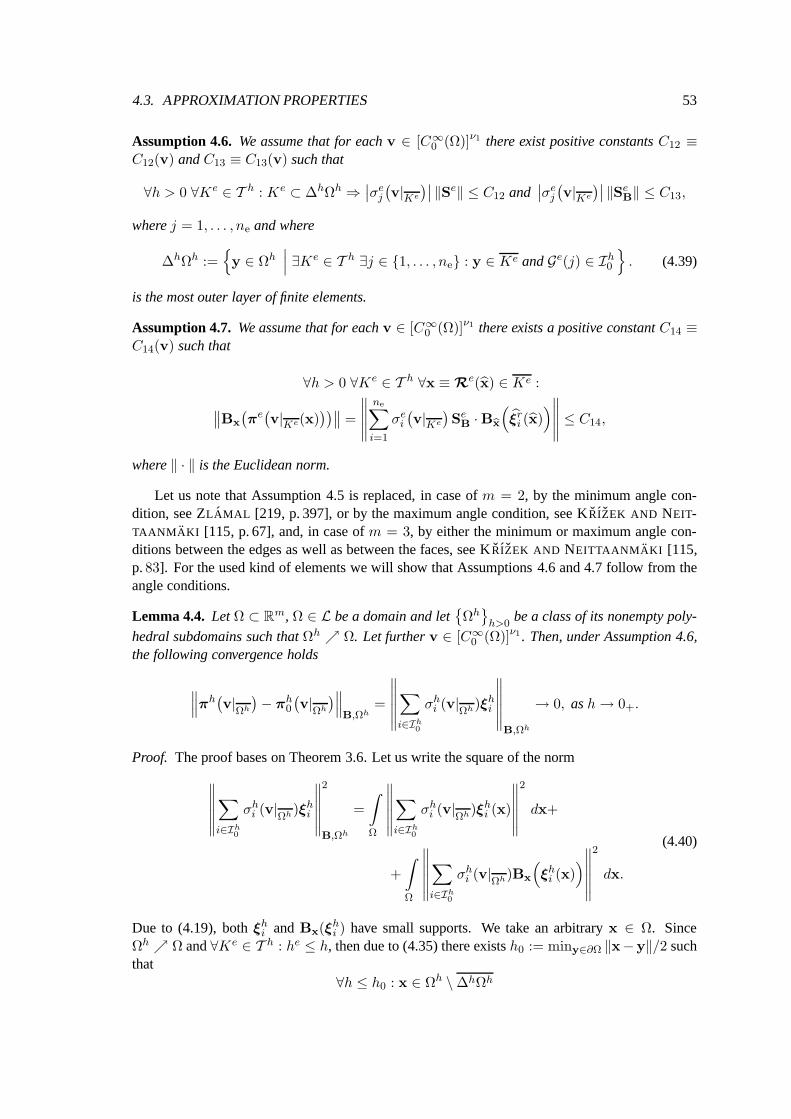
4.3. APPROXIMATION PROPERTIES 53
Assumption 4.6. We assume that for each v ∈ [C∞0 (Ω)]ν1 there exist positive constants C12 ≡
C12(v) and C13 ≡ C13(v) such that
∀h > 0 ∀Ke ∈ T h : Ke ⊂ ∆hΩh ⇒∣∣σe
j
(v|Ke
)∣∣ ‖Se‖ ≤ C12 and∣∣σe
j
(v|Ke
)∣∣ ‖SeB‖ ≤ C13,
where j = 1, . . . , ne and where
∆hΩh :=y ∈ Ωh
∣∣∣ ∃Ke ∈ T h ∃j ∈ 1, . . . , ne : y ∈ Ke and Ge(j) ∈ Ih0
. (4.39)
is the most outer layer of finite elements.
Assumption 4.7. We assume that for each v ∈ [C∞0 (Ω)]ν1 there exists a positive constant C14 ≡
C14(v) such that
∀h > 0 ∀Ke ∈ T h ∀x ≡ Re(x) ∈ Ke :
∥∥Bx
(πe(v|Ke(x)
))∥∥ =
∥∥∥∥∥ne∑
i=1
σei
(v|Ke
)Se
B ·Bbx
(ξr
i (x))∥∥∥∥∥ ≤ C14,
where ‖ · ‖ is the Euclidean norm.
Let us note that Assumption 4.5 is replaced, in case of m = 2, by the minimum angle con-dition, see ZLAMAL [219, p. 397], or by the maximum angle condition, see K RIZEK AND NEIT-TAANMAKI [115, p. 67], and, in case of m = 3, by either the minimum or maximum angle con-ditions between the edges as well as between the faces, see K RIZEK AND NEITTAANMAKI [115,p. 83]. For the used kind of elements we will show that Assumptions 4.6 and 4.7 follow from theangle conditions.
Lemma 4.4. Let Ω ⊂ Rm, Ω ∈ L be a domain and letΩh
h>0be a class of its nonempty poly-
hedral subdomains such that Ωh Ω. Let further v ∈ [C∞0 (Ω)]ν1 . Then, under Assumption 4.6,
the following convergence holds
∥∥∥πh(v|
Ωh
)− πh
0
(v|
Ωh
)∥∥∥B,Ωh
=
∥∥∥∥∥∥∑
i∈Ih0
σhi (v|
Ωh)ξhi
∥∥∥∥∥∥B,Ωh
→ 0, as h → 0+.
Proof. The proof bases on Theorem 3.6. Let us write the square of the norm
∥∥∥∥∥∥∑
i∈Ih0
σhi (v|
Ωh)ξhi
∥∥∥∥∥∥
2
B,Ωh
=
∫
Ω
∥∥∥∥∥∥∑
i∈Ih0
σhi (v|
Ωh)ξhi (x)
∥∥∥∥∥∥
2
dx+
+
∫
Ω
∥∥∥∥∥∥∑
i∈Ih0
σhi (v|
Ωh)Bx
(ξh
i (x))∥∥∥∥∥∥
2
dx.
(4.40)
Due to (4.19), both ξhi and Bx(ξh
i ) have small supports. We take an arbitrary x ∈ Ω. SinceΩh Ω and ∀Ke ∈ T h : he ≤ h, then due to (4.35) there exists h0 := miny∈∂Ω ‖x−y‖/2 suchthat
∀h ≤ h0 : x ∈ Ωh \ ∆hΩh
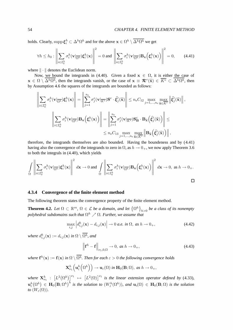
54 CHAPTER 4. FINITE ELEMENT METHOD
holds. Clearly, suppξhi ⊂ ∆hΩh and for the above x ∈ Ωh \ ∆hΩh we get
∀h ≤ h0 :
∥∥∥∥∥∥∑
i∈Ih0
σhi (v|
Ωh)ξhi (x)
∥∥∥∥∥∥
2
= 0 and
∥∥∥∥∥∥∑
i∈Ih0
σhi (v|
Ωh)Bx
(ξh
i (x))∥∥∥∥∥∥
2
= 0, (4.41)
where ‖ · ‖ denotes the Euclidean norm.Now, we bound the integrands in (4.40). Given a fixed x ∈ Ω, it is either the case of
x ∈ Ω \ ∆hΩh, then the integrands vanish, or the case of x ≡ Re(x) ∈ Ke ⊂ ∆hΩh, thenby Assumption 4.6 the squares of the integrands are bounded as follows:
∥∥∥∥∥∥∑
i∈Ih0
σhi (v|
Ωh)ξhi (x)
∥∥∥∥∥∥=
∥∥∥∥∥∥
ne∑
j=1
σej (v|Ke)S
e · ξrj(x)
∥∥∥∥∥∥≤ neC12 max
j=1,...,ne
maxbx∈Kr
∥∥∥ξrj(x)
∥∥∥ ,
∥∥∥∥∥∥∑
i∈Ih0
σhi (v|
Ωh)Bx
(ξh
i (x))∥∥∥∥∥∥
=
∥∥∥∥∥∥
ne∑
j=1
σej (v|Ke)S
eB ·Bbx
(ξr
j(x))∥∥∥∥∥∥≤
≤ neC13 maxj=1,...,ne
maxbx∈Kr
∥∥∥Bbx
(ξr
j(x))∥∥∥ ,
therefore, the integrands themselves are also bounded. Having the boundeness and by (4.41)having also the convergence of the integrands to zero in Ω, as h → 0+, we now apply Theorem 3.6to both the integrals in (4.40), which yields
∫
Ω
∥∥∥∥∥∥∑
i∈Ih0
σhi (v|
Ωh)ξhi (x)
∥∥∥∥∥∥
2
dx → 0 and∫
Ω
∥∥∥∥∥∥∑
i∈Ih0
σhi (v|
Ωh)Bx
(ξh
i (x))∥∥∥∥∥∥
2
dx → 0, as h → 0+.
4.3.4 Convergence of the finite element method
The following theorem states the convergence property of the finite element method.
Theorem 4.2. Let Ω ⊂ Rm, Ω ∈ L be a domain, and letΩh
h>0be a class of its nonempty
polyhedral subdomains such that Ωh Ω. Further, we assume that
maxi,j
∣∣∣dhi,j(x) − di,j(x)
∣∣∣→ 0 a.e. in Ω, as h → 0+, (4.42)
where dhi,j(x) := di,j(x) in Ω \ Ωh, and
∥∥∥fh − f
∥∥∥ν1,0,Ω
→ 0, as h → 0+, (4.43)
where fh(x) := f(x) in Ω \ Ωh. Then for each ε > 0 the following convergence holds
Xhν1
(uh
ε
(Ωh))
→ uε(Ω) in H0(B; Ω), as h → 0+,
where Xhν1
:[L2(Ωh)]ν1 7→
[L2(Ω)
]ν1 is the linear extension operator defined by (4.33),
uhε
(Ωh)∈ H0
(B; Ωh
)his the solution to (W h
ε (Ωh)), and uε(Ω) ∈ H0(B; Ω) is the solutionto (Wε(Ω)).
4.3. APPROXIMATION PROPERTIES 55
Proof. Let ε > 0 be arbitrary. Let us denote
uε := uε(Ω) and uhε := Xh
ν1
(uh
ε
(Ωh))
. (4.44)
From Lemma 4.3 we know that the set X0
(B; Ω;Ωh
)his a closed subspace of H0(B; Ω). There-
fore, the function uhε is the Galerkin approximation to the solution uε of (Wε(Ω)) in the space
X0
(B; Ω;Ωh
)hand we can employ Lemma 4.1, which for any vh ∈ X0
(B; Ω;Ωh
)hyields
∥∥∥uε − uhε
∥∥∥B,Ω
≤ C9(ε)
∥∥∥uε − vh∥∥∥B,Ω
+
∣∣aε
(vh,uh
ε − vh)− ah
ε
(vh,uh
ε − vh)∣∣
‖uhε − vh‖B,Ω
+
+
∣∣f(uh
ε − vh)− fh
(uh
ε − vh)∣∣
‖uhε − vh‖B,Ω
.
(4.45)
Now the idea of the proof is like in KRIZEK AND NEITTAANMAKI [115, Th. 4.16], originallyfrom DOKTOR [56]. Let τ > 0 be arbitrary. By Assumption 3.3, there exists uε ∈ [C∞
0 (Ω)]ν1
such that‖uε(Ω) − uε‖B,Ω ≤ τ
6C9(ε). (4.46)
In the estimate (4.45) we choose
vh := Xhν1
(πh
0
(uε|Ωh
)).
We estimate the first term on the right–hand side of (4.45). By the triangle inequality (3.1),by Lemma 4.3, and by (4.46), we get
∥∥∥uε − vh∥∥∥B,Ω
=∥∥∥uε − uε + uε − vh
∥∥∥B,Ω
≤ ‖uε − uε‖B,Ω +∥∥∥uε − vh
∥∥∥B,Ω
≤
≤ τ
6C9(ε)+∥∥∥uε − vh
∥∥∥B,Ω
.(4.47)
The second term on the right–hand side of (4.47) reads
∥∥∥uε − vh∥∥∥
2
B,Ω=
∫
ΩχΩ\Ωh(x)
(‖uε(x)‖2 + ‖B (uε(x))‖2
)dx +
∥∥∥uε − πh0
(uε|Ωh
)∥∥∥2
B,Ωh=
=
∫
Ω(1 − χΩh(x))
(‖uε(x)‖2 + ‖B (uε(x))‖2
)dx +
∥∥∥uε − πh0
(uε|Ωh
)∥∥∥2
B,Ωh,
(4.48)where ‖ · ‖ denotes the Euclidean norm. Since Ωh Ω, then (4.35) holds and we get
(1 − χΩh(x))(‖uε(x)‖2 + ‖B(uε(x))‖2
)→ 0 a.e. in Ω, as h → 0+.
Moreover, due to (4.36)
∀h > 0 : (1 − χΩh(x))(‖uε(x)‖2 + ‖B(uε(x))‖2
)≤ ‖uε(x)‖2 + ‖B(uε(x))‖2 a.e. in Ω.
Therefore, Theorem 3.6 yields∫
Ω
(1 − χΩh(x))(‖uε(x)‖2 + ‖B(uε(x))‖2
)dx → 0, as h → 0+.
56 CHAPTER 4. FINITE ELEMENT METHOD
Using the triangle inequality (3.1), the second term on the right–hand side of (4.48) is estimatedas follows:
∥∥∥uε − πh0
(uε|Ωh
)∥∥∥B,Ωh
=∥∥∥uε − πh
(uε|Ωh
)+ πh
(uε|Ωh
)− πh
0
(uε|Ωh
)∥∥∥B,Ωh
≤
≤∥∥∥uε − πh
(uε|Ωh
)∥∥∥B,Ωh
+∥∥∥πh
(uε|Ωh
)− πh
0
(uε|Ωh
)∥∥∥B,Ωh
.
(4.49)The definition (4.38), Assumption 4.4, and Assumption 4.5, respectively, yield
∥∥∥uε − πh(uε|Ωh
)∥∥∥2
B,Ωh=
∑
Ke∈T h
‖uε − πe(uε|Ke)‖2B,Ke ≤
≤∑
Ke∈T h
(C10(K
e)he ‖uε‖ν1,2,Ke
)2≤ C2
11h2 ‖uε‖2
ν1,2,Ω .
By Lemma 4.4, the second term on the right–hand side of (4.49) tends toward zero. Therefore, theright–hand side of (4.48) tends to zero, as h → 0+, i.e., there exists h1 > 0 such that
∀h ≤ h1 :∥∥∥uε − vh
∥∥∥B,Ω
≤ τ
3C9(ε). (4.50)
Further, we estimate the second term on the right–hand side of (4.45). The nominator reads asfollows:∣∣∣aε
(vh,uh
ε − vh)− ah
ε
(vh,uh
ε − vh)∣∣∣ =
=
∣∣∣∣∫
ΩB(uh
ε − vh)·((
D −Dh)T
· B(vh))
dx
∣∣∣∣ ≤
≤∣∣∣uh
ε − vh∣∣∣B,Ω
√∫
Ωmax
i,j
∣∣∣dhi,j(x) − di,j(x)
∣∣∣2‖B(vh(x))‖2
dx,
where we used the Cauchy–Schwarz inequality (3.3) in[L2(Ω)
]ν2 . After dividing the latter by∥∥uhε − vh
∥∥B,Ω
, we get
∣∣aε
(vh,uh
ε − vh)− ah
ε
(vh,uh
ε − vh)∣∣
‖uhε − vh‖B,Ω
≤√∫
Ωmax
i,j
∣∣∣dhi,j(x) − di,j(x)
∣∣∣2‖B(vh(x))‖2
dx.
(4.51)Now, we use Theorem 3.6 to show that the integral on the right–hand side of (4.51) vanishes, ash → 0+. First, we prove the boundeness of the integrand. We take an arbitrary x ∈ Ω. If x 6∈ Ωh,then vh(x) = 0 and the integrand vanishes. If x ∈ K e for some Ke ∈ T h, Ke ⊂ ∆hΩh, thenby (4.3) and Assumption 4.6 the square of the integrand reads
maxi,j
∣∣∣dhi,j(x) − di,j(x)
∣∣∣∥∥∥B(vh(x)
)∥∥∥ =
= maxi,j
∣∣∣dhi,j(x) − di,j(x)
∣∣∣
∥∥∥∥∥∥∑
j:Ge(j)6∈Ih0
σej
(uε|Ke
)Se
B · Bbx
(ξr
j(x))∥∥∥∥∥∥≤
≤ 2maxi,j
‖di,j‖L∞(Ω) neC13(uε) maxj=1,...,ne
maxbx∈Kr
∥∥∥Bbx
(ξr
j(x))∥∥∥ .

4.4. FINITE ELEMENTS FOR MAGNETOSTATICS 57
Otherwise, x ∈ Ke for some Ke ∈ T h, Ke ⊂ Ωh \ ∆hΩh, and the square of the integrand reads
maxi,j
∣∣∣dhi,j(x) − di,j(x)
∣∣∣∥∥∥B(vh(x)
)∥∥∥ =
= maxi,j
∣∣∣dhi,j(x) − di,j(x)
∣∣∣
∥∥∥∥∥∥
ne∑
j=1
σej
(uε|Ke
)Se
B · Bbx
(ξr
j(x))∥∥∥∥∥∥≤
≤ 2maxi,j
‖di,j‖L∞(Ω) C14(uε) ,
where we used (4.3) and Assumption 4.7. Therefore, the integrand on the right–hand side of (4.51)is bounded by a constant independent of h, and due to the assumption (4.42) it converges to zeroalmost everywhere in Ω. Then, by Theorem 3.6
∫
Ωmax
i,j
∣∣∣dhi,j − di,j
∣∣∣2 ∥∥∥B
(vh)∥∥∥
2dx → 0, as h → 0+.
Hence, there exists h2 > 0 such that
∀h ≤ h2 :
∣∣aε
(vh,uh
ε − vh)− ah
ε
(vh,uh
ε − vh)∣∣
‖uhε − vh‖B,Ω
≤ τ
3C9(ε). (4.52)
Finally, we estimate the third term on the right–hand side of (4.45). The nominator reads asfollows:
∣∣∣f(uh
ε − vh)− fh
(uh
ε − vh)∣∣∣ =
∣∣∣∣∫
Ω
(f − fh
)·(uh
ε − vh)
dx
∣∣∣∣ ≤
≤∥∥∥f − fh
∥∥∥ν1,0,Ω
∥∥∥uhε − vh
∥∥∥ν1,0,Ω
≤
≤∥∥∥f − fh
∥∥∥ν1,0,Ω
∥∥∥uhε − vh
∥∥∥B,Ω
,
(4.53)
where we used the Cauchy–Schwarz inequality in[L2(Ω)
]ν1 . Dividing (4.53) by∥∥uh
ε − vh∥∥B,Ω
and using the assumption (4.43), it follows that there exists h3 > 0 such that
∀h ≤ h3 :
∣∣f(uh
ε − vh)− fh
(uh
ε − vh)∣∣
‖uhε − vh‖B,Ω
≤ τ
3C9(ε). (4.54)
At the end, combining (4.45), (4.50), (4.52), and (4.54), and recalling the notation (4.44), we haveproven the statement, i.e., for any τ > 0 there exists h0 := minh1, h2, h3 such that
∀h ≤ h0 :∥∥∥uε(Ω) −Xh
ν1
(uh
ε
(Ωh))∥∥∥
B,Ω≤ τ.
4.4 Finite elements for magnetostatics
In this section, we derive two basic types of finite elements which are used for solving the 2–dimensional or 3–dimensional magnetostatic problem, respectively. We will validate Assump-tions 4.1–4.2 and Assumptions 4.4–4.7.
58 CHAPTER 4. FINITE ELEMENT METHOD
4.4.1 Linear Lagrange elements on triangles
These finite elements approximate the space H1(Ω), where Ω ⊂ R2, Ω ∈ L. They are used,e.g., for solving the 2–dimensional linear magnetostatic problem introduced in Section 3.4.2. Theelements are characterized by triangular domains and by the degrees of freedom that are nodalvalues in the corners.
The linear Lagrange element is a triple E :=(Ke, P e,Σe
), where Ke ⊂ R2 is a triangular
domain,
P e :=
p(x) := ae0 + ae
1x1 + ae2x2 ∈ C
(Ke) ∣∣ ae
0, ae1, a
e2 ∈ R , x := (x1, x2) ∈ Ke
,
and the degrees of freedom are
Σe := σe1, σ
e2, σ
e3 ,
where σei : C
(Ke)7→ R is such that for v ∈ C
(Ke)
σei (v) := v(xe
i ) , i = 1, 2, 3, (4.55)
where xe1 :=
(xe
1,1, xe1,2
), xe
2 :=(xe
2,1, xe2,2
), xe
3 :=(xe
3,1, xe3,2
)are the corners of Ke.
We concern the space H1(Ke) with the trace operator γKe(v) := v|∂Ke , v ∈ P e. From (4.55)it is easy to see that the following couples of degrees of freedom (σe
1, σe2), (σe
2, σe3), and (σe
3, σe1)
for any v ∈ P e determine the traces v|he3, v|he
2, and v|he
1along the edges he
3 := (xe1,x
e2), he
1 :=(xe
2,xe3), and he
2 := (xe3,x
e1), respectively, see also Fig. 4.4. Therefore, Assumption 4.1 is fulfilled
and we say that the linear Lagrange elements are H 1(Ke)–conforming.According to (4.27), (4.28), and Fig. 4.2, we specify the transformation from the reference
element to the element e by
Re :=
(xe
2,1 − xe1,1 xe
3,1 − xe1,1
xe2,2 − xe
1,2 xe3,2 − xe
1,2
), re :=
(xe
1,1
xe1,2
), (4.56)
where the corners of the reference triangle K r are
xr1 := (0, 0), xr
2 := (1, 0), xr3 := (0, 1). (4.57)
Concerning Assumption 4.2, we specify Se by
Se := 1. (4.58)
It is easy to see that
gradx(v(x)) = (Re)−T · gradbx(v(x)) , (4.59)
where v(x) := Se · v(x) and x := Re · x + re. The reference shape functions read as follows:
ξr1(x) := 1 − x1 − x2, ξr
2(x) := x1, ξr3(x) := x2, where x := (x1, x2) ∈ Kr (4.60)
and where Kr is the triangle in Fig. 4.2 the corners of which are given by (4.57).Now we will state the element approximation property such that both Assumption 4.4 and
Assumption 4.5 will be fulfilled. Suppose that we have a discretization T h :=Ke1 , . . . ,K
enΩh
– a triangulation. The following definition is due to ZLAMAL [219, p. 397].
4.4. FINITE ELEMENTS FOR MAGNETOSTATICS 59
Definition 4.1. A family F :=T h | h > 0
of triangulations is said to satisfy the minimum
angle condition if there exists a constant γ0 such that for any T h ∈ F and any Ke ∈ T h we have
0 < γ0 ≤ γKe <π
2, (4.61)
where γKe is the minimum angle of the triangle Ke.
The next lemma is due to ZLAMAL [219] and it replaces both Assumption 4.4 and Assump-tion 4.5.
Lemma 4.5. Let F be a family of triangulations satisfying the minimum angle condition (4.61).Then there exists a constant C11 > 0 such that for any T h ∈ F with h ≤ h we have
∀v ∈ H2(Ωh)
:∥∥∥v − πh(v)
∥∥∥1,Ωh
≤ C11h |v|2,Ωh ,
where πh : C(Ωh)7→ H1
(Ωh)h
is defined by (4.38), using the degrees of freedom (4.55).
Proof. See ZLAMAL [219].
The next two lemmas fulfill Assumptions 4.6 and 4.7, respectively.
Lemma 4.6. Let v ∈ C∞0 (Ω). Then there exist positive constants C12 ≡ C12(v) and C13 ≡
C13(v) such that for any discretization parameter h > 0 satisfying (4.32), for any subdomainΩh ⊂ Ω satisfying Assumption 4.3, and for any discretization T h which satisfies the minimumangle condition (4.61) the following holds
∀Ke ∈ T h : Ke ⊂ ∆hΩh ⇒∣∣σe
j
(v|Ke
)∣∣ ‖Se‖ ≤ C12 and∣∣σe
j
(v|Ke
)∣∣ ∥∥Segrad
∥∥ ≤ C13,
where j = 1, 2, 3 and where ∆hΩh is defined by (4.39).
Proof. Let v ∈ C∞0 (Ω) be an arbitrary function, h > 0 be a discretization parameter satisfy-
ing (4.32), Ωh ⊂ Ω be a polygonal subdomain satisfying Assumption 4.3, and T h be a discretiza-tion which satisfies the minimum angle condition (4.61).
Let Ke ⊂ Ωh be arbitrary and let x ∈ Ke. Since Se = 1, the first estimate is as follows:∣∣σe
j
(v|Ke
)∣∣ ‖Se‖ =∣∣v(xe
j
)∣∣ ≤ maxz∈Ω
|v(z)| , j = 1, 2, 3,
where xej ∈ ∂Ke is a corner of Ke. Hence,
C12 := maxz∈Ω
|v(z)| .
Let now Ke ∈ T h be such that Ke ⊂ ∆hΩh and let x ∈ Ke. Then, by Assumption 4.3, thereexist y ∈ ∂Ω and xh ∈ ∂Ωh such that
‖x − y‖ =∥∥∥x− xh + xh − y
∥∥∥ ≤∥∥∥x− xh
∥∥∥+∥∥∥xh − y
∥∥∥ ≤ 2he,
where he is by definition the maximum side of Ke. Since y ∈ ∂Ω, then v(y) = 0. Now, we useTheorem 3.3
v(x) = v(y) + grad(v(z)) · (x − z) = grad(v(z)) · (x− z), (4.62)
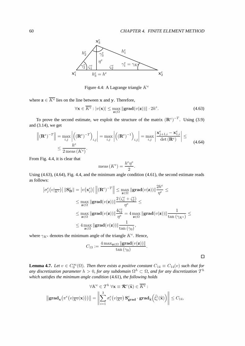
60 CHAPTER 4. FINITE ELEMENT METHOD
PSfrag replacements
he1he
2
he3 = he
γe1 = γKeγe
2
γe3
xe1 xe
2
xe3
ηe
ζe1 ζe
2
Figure 4.4: A Lagrange triangle Ke
where z ∈ Ke lies on the line between x and y. Therefore,
∀x ∈ Ke : |v(x)| ≤ maxz∈Ω
‖grad(v(z))‖ · 2he. (4.63)
To prove the second estimate, we exploit the structure of the matrix (Re)−T . Using (3.9)and (3.14), we get
∥∥∥(Re)−T∥∥∥ = max
i,j
∣∣∣∣((Re)−T
)i,j
∣∣∣∣ = maxi,j
∣∣∣∣((Re)−1
)i,j
∣∣∣∣ = maxi,j
∣∣∣∣xe
j+1,i − xe1,i
det (Re)
∣∣∣∣ ≤
≤ he
2meas (Ke).
(4.64)
From Fig. 4.4, it is clear that
meas (Ke) =heηe
2.
Using (4.63), (4.64), Fig. 4.4, and the minimum angle condition (4.61), the second estimate readsas follows:
∣∣σej
(v|Ke
)∣∣ ‖SeB‖ =
∣∣v(xe
j
)∣∣∥∥∥(Re)−T
∥∥∥ ≤ maxz∈Ω
‖grad(v(z))‖2he
ηe≤
≤ maxz∈Ω
‖grad(v(z))‖2 (ζe1 + ζe
2)
ηe≤
≤ maxz∈Ω
‖grad(v(z))‖4ζe2
ηe= 4max
z∈Ω‖grad(v(z))‖ 1
tan (γKe)≤
≤ 4maxz∈Ω
‖grad(v(z))‖ 1
tan (γ0),
where γKe denotes the minimum angle of the triangle K e. Hence,
C13 :=4maxz∈Ω ‖grad(v(z))‖
tan (γ0).
Lemma 4.7. Let v ∈ C∞0 (Ω). Then there exists a positive constant C14 ≡ C14(v) such that for
any discretization parameter h > 0, for any subdomain Ωh ⊂ Ω, and for any discretization T h
which satisfies the minimum angle condition (4.61), the following holds
∀Ke ∈ T h ∀x ≡ Re(x) ∈ Ke :
∥∥gradx
(πe(v|Ke(x)
))∥∥ =
∥∥∥∥∥3∑
i=1
σei
(v|Ke
)Se
grad · gradbx
(ξri (x)
)∥∥∥∥∥ ≤ C14,
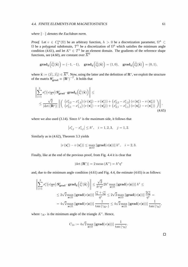
4.4. FINITE ELEMENTS FOR MAGNETOSTATICS 61
where ‖ · ‖ denotes the Euclidean norm.
Proof. Let v ∈ C∞0 (Ω) be an arbitrary function, h > 0 be a discretization parameter, Ωh ⊂
Ω be a polygonal subdomain, T h be a discretization of Ωh which satisfies the minimum anglecondition (4.61), and let Ke ∈ T h be an element domain. The gradients of the reference shapefunctions, see (4.60), are constant over Kr
gradbx
(ξr1(x)
)= (−1,−1), gradbx
(ξr2(x)
)= (1, 0), gradbx
(ξr3(x)
)= (0, 1),
where x := (x1, x2) ∈ Kr. Now, using the latter and the definition of Re, we exploit the structureof the matrix Se
grad ≡ (Re)−T . It holds that
∥∥∥∥∥3∑
i=1
σei
(v|Ke
)Se
grad · gradbx
(ξri (x)
)∥∥∥∥∥ ≤
≤√
2
|det (Re)|
∥∥∥∥( (
xe3,2 − xe
1,2
)(v (xe
2) − v (xe1)) +
(xe
2,2 − xe1,2
)(v (xe
1) − v (xe3))(
xe3,1 − xe
1,1
)(v (xe
1) − v (xe2)) +
(xe
2,1 − xe1,1
)(v (xe
3) − v (xe1))
)∥∥∥∥ ,
(4.65)
where we also used (3.14). Since he is the maximum side, it follows that
∣∣xei,j − xe
1,j
∣∣ ≤ he, i = 1, 2, 3, j = 1, 2.
Similarly as in (4.62), Theorem 3.3 yields
|v (xei ) − v (xe
1)| ≤ maxz∈Ω
‖grad(v(z))‖ he, i = 2, 3.
Finally, like at the end of the previous proof, from Fig. 4.4 it is clear that
|det (Re)| = 2meas (Ke) = heηe
and, due to the minimum angle condition (4.61) and Fig. 4.4, the estimate (4.65) is as follows:
∥∥∥∥∥3∑
i=1
σei
(v|Ke
)Se
grad · gradbx
(ξri (x)
)∥∥∥∥∥ ≤√
2
heηe2he max
z∈Ω‖grad(v(z))‖ he ≤
≤ 2√
2 maxz∈Ω
‖grad(v(z))‖ ζe1 + ζe
2
ηe≤ 2
√2max
z∈Ω‖grad(v(z))‖ 2ζe
2
ηe=
= 4√
2 maxz∈Ω
‖grad(v(z))‖ 1
tan (γKe)≤ 4
√2 max
z∈Ω‖grad(v(z))‖ 1
tan (γ0),
where γKe is the minimum angle of the triangle Ke. Hence,
C14 := 4√
2 maxz∈Ω
‖grad(v(z))‖ 1
tan (γ0).
62 CHAPTER 4. FINITE ELEMENT METHOD
PSfrag replacements
0
1
1
1
x1
x2
x3
cr1
cr2
cr3
cr4
cr5
cr6
Kr
Re
x1
x2
x3
ce1
ce2
ce3
ce4
ce5
ce6
Ke
Figure 4.5: A transformation from the reference Nedelec tetrahedron
4.4.2 Linear Nedelec elements on tetrahedra
Here, we state a type of finite elements, which is frequently used for the approximation of the spaceH(curl; Ω), where Ω ⊂ R3, Ω ∈ L. These elements can be used for solving the 3–dimensionallinear magnetostatic problem, which was introduced in Section 3.4.3. The elements are definedover tetrahedra and the degrees of freedom are calculated as integrals along the edges. The el-ements were first introduced by NEDELEC [142] and, since then, they have become a standard.
The linear Nedelec element is a triple E :=(Ke,Pe,Σe
), where Ke ⊂ R3 is a tetrahedral
domain,
Pe :=p(x) := ae × x + be
∣∣ ae,be ∈ R3, x := (x1, x2, x3) ∈ Ke
,
and the degrees of freedom are
Σe := σe1, σ
e2, σ
e3, σ
e4, σ
e5, σ
e6 ,
where σei :[C(Ke)]3 7→ R is such that for v ∈
[C(Ke)]3
σei (v) :=
∫
cei
v · tei ds, i = 1, . . . , 6,
where cei stand for the oriented edges, see Fig. 4.5, and te
i are the related unit tangential vectors.Now, we concern the space H(curl;Ke) and the corresponding trace operator γKe(v) :=
ne × v on ∂Ke, where v ∈ Pe and ne denotes the unit outer normal vector to ∂K e. By NE-DELEC [142, Theorem 1], Assumption 4.1 is fulfilled, thus, the linear Nedelec finite elements areH(curl;Ke)–conforming.
The transformation Re in Fig. 4.5 is determined by
Re :=
xe2,1 − xe
1,1 xe3,1 − xe
1,1 xe4,1 − xe
1,1
xe2,2 − xe
1,2 xe3,2 − xe
1,2 xe4,2 − xe
1,2
xe2,3 − xe
1,3 xe3,3 − xe
1,3 xe4,3 − xe
1,3
, re :=
xe1,1
xe1,2
xe1,3
, (4.66)
where xei :=
(xe
i,1, xei,2, x
ei,3
), i=1,. . . ,4, are the corners of the tetrahedron K e, which correspond
to the following corners of Kr
xr1 := (0, 0, 0), xr
2 := (1, 0, 0), xr3 := (0, 1, 0), xr
4 := (0, 0, 1). (4.67)
4.4. FINITE ELEMENTS FOR MAGNETOSTATICS 63
As far as Assumption 4.2 is considered, we determine Se by
Se := (Re)−T . (4.68)
It can be shown that following Piola’s transformation holds, see RAVIART AND THOMAS [167,Formula 3.17],
curlx(v(x)) =1
det(Re)Re · curlbx(v(x)) , (4.69)
where v(x) := Se · v(x) and x := Re · x + re. The reference shape functions read as follows:
ξr1(x) :=
0−1
1
× x +
100
, ξr
2(x) :=
10
−1
× x +
010
,
ξr3(x) :=
−110
× x +
001
, ξr
4(x) :=
001
× x +
000
,
ξr5(x) :=
100
× x +
000
, ξr
6(x) :=
010
× x +
000
,
(4.70)
where x := (x1, x2, x3) ∈ Kr and Kr is the reference tetrahedron, see Fig. 4.5, the corners ofwhich are given by (4.67).
Now, we will state the element approximation property such that both Assumption 4.4 and As-sumption 4.5 will be fulfilled. Suppose that we have a decomposition T h :=
Ke1 , . . . ,K
enΩh
.The following definition and lemma are due to N EDELEC [142, p. 327].
Definition 4.2. A family F :=T h | h > 0
of decompositions into tetrahedra is said to be
regular if there exists a constant C15 > 0 such that for any T h ∈ F and any Ke ∈ T h we have
he
ρe≤ C15, (4.71)
where ρe denotes the radius of the largest sphere inscribed in K e.
Lemma 4.8. Let F be a regular family of decompositions into tetrahedra in the sense of Def-inition 4.2. Then there exists a constant C11 > 0 such that for any T h ∈ F with h ≤ h wehave
∀v ∈[H2(Ωh)]ν1
: ‖v − πe(v)‖curl,Ωh ≤ C11h |v|ν1,2,Ωh .
Proof. The assertion is a direct consequence of N EDELEC [142, Th. 2].
The next two lemmas fulfill Assumptions 4.6 and 4.7, respectively.
Lemma 4.9. Let v ∈ [C∞0 (Ω)]3. Then there exist positive constants C12 ≡ C12(v) and C13 ≡
C13(v) such that for any discretization parameter h > 0, for any subdomain Ωh ⊂ Ω satisfyingAssumption 4.3, and for any discretization T h which satisfies the regularity condition (4.71) thefollowing holds
∀Ke ∈ T h : Ke ⊂ ∆hΩh ⇒∣∣σe
j
(v|Ke
)∣∣ ‖Se‖ ≤ C12 and∣∣σe
j
(v|Ke
)∣∣ ‖Securl‖ ≤ C13,
where j = 1, . . . , 6.
64 CHAPTER 4. FINITE ELEMENT METHOD
Proof. Let v := (v1, . . . , vν1) ∈ [C∞
0 (Ω)]ν1 be an arbitrary function, h > 0 be a discretizationparameter satisfying (4.32), Ωh ⊂ Ω be a polygonal subdomain satisfying Assumption 4.3, T h
be a discretization which satisfies the regularity condition (4.71), and let Ke ∈ T h be an elementdomain. For j = 1, . . . , 6 we have the estimate
∣∣σej
(v|Ke
))∣∣ =
∣∣∣∣∣
∫
cej
v(x) · tej ds
∣∣∣∣∣ ≤ maxz∈Ω
‖v(z)‖ he, (4.72)
where he stands for the maximum edge size. Since Se := (Re)−T , then, using (3.9) and (3.14), itfollows that
‖Se‖ =1
|det (Re)|∥∥∥Re
∥∥∥ =1
6meas (Ke)
∥∥∥Re∥∥∥ ≤ (he)2
3meas (Ke). (4.73)
Since ρe denotes the radius of the largest sphere inscribed in K e, from the regularity condi-tion (4.71) it is obvious that
meas (Ke) ≥ 4
3π (ρe)3 ≥ 4
3π
(he
C15
)3
. (4.74)
Putting the latter into (4.73) and combining that with (4.72), the first estimate reads as follows:
∣∣σej
(v|Ke
)∣∣ ‖Se‖ ≤ maxz∈Ω
‖v(z)‖ (C15)3
4π,
hence,
C12 := maxz∈Ω
‖v(z)‖ (C15)3
4π.
Similarly as in the proof of Lemma 4.6, let Ke ∈ T h be such that Ke ⊂ ∆hΩh. Then thereexists xh ∈ ∂Ωh and, by Assumption 4.3, there exists y ∈ ∂Ω such that
‖x − y‖ =∥∥∥x − xh + xh − y
∥∥∥ ≤∥∥∥x− xh
∥∥∥+∥∥∥xh − y
∥∥∥ ≤ 2he,
where he is by definition the maximum side of Ke. Since y ∈ ∂Ω, then v(y) = 0. Now we useTheorem 3.3
vi(x) = vi(y) + grad(vi(z)) · (x − z) = grad(vi(z)) · (x − z) for i = 1, 2, 3
and‖v(x)‖ ≤ max
i∈1,2,3maxz∈Ω
‖grad(vi(z))‖ 2he for i = 1, 2, 3,
where z ∈ Ke lies on the line between x and y. Therefore,
∣∣σej
(v|Ke
)∣∣ =
∣∣∣∣∣
∫
cej
v(x) · tej ds
∣∣∣∣∣ ≤ maxi∈1,2,3
maxz∈Ω
‖grad(vi(z))‖ 2 (he)2 . (4.75)
Concerning the second estimate, we have
‖Securl‖ =
1
|det (Re)| ‖Re‖ ≤
maxi,j
∣∣∣xei+1,j − xe
1,j
∣∣∣6meas (Ke)
≤ he
6meas (Ke)≤ (C15)
3
8π (he)2,
4.4. FINITE ELEMENTS FOR MAGNETOSTATICS 65
where we used (4.74). Combining the latter with (4.75), the second estimate is as follows:
∣∣σej
(v|Ke
)∣∣ ‖Securl‖ ≤ max
i∈1,2,3maxz∈Ω
‖grad(vi(z))‖ 2 (he)2(C15)
3
8π (he)2≤
≤ 1
4max
i∈1,2,3maxz∈Ω
‖grad(vi(z))‖ (C15)3 ,
(4.76)
hence,
C13 :=1
4max
i∈1,2,3maxz∈Ω
‖grad(vi(z))‖ (C15)3 .
Lemma 4.10. Let v ∈ [C∞0 (Ω)]3. Then there exists a positive constant C14 ≡ C14(v) such that
for any discretization parameter h > 0, for any subdomain Ωh ⊂ Ω, and for any discretizationT h which satisfy the regularity condition (4.71), the following holds
∀Ke ∈ T h ∀x ≡ Re(x) ∈ Ke :
∥∥curlx(πe(v|Ke
))∥∥ =
∥∥∥∥∥6∑
i=1
σei
(v|Ke
)Se
curl · curlbx
(ξr
i (x))∥∥∥∥∥ ≤ C14. (4.77)
Proof. The proof is similar to that of Lemma 4.7. Let v ∈ [C∞0 (Ω)]ν1 be an arbitrary function,
h > 0 be a discretization parameter, Ωh ⊂ Ω be a polygonal subdomain, T h be a discretization ofΩh which satisfies the regularity condition (4.71), and let Ke ∈ T h be an element domain. Therotations of the reference shape functions, see (4.70), are constant over Kr
curlbx
(ξr
1(x))
= (0,−2, 2), curlbx
(ξr
2(x))
= (2, 0,−2), curlbx
(ξr
3(x))
= (−2, 2, 0),
curlbx
(ξr
4(x))
= (0, 0, 2), curlbx
(ξr
5(x))
= (2, 0, 0), curlbx
(ξr
6(x))
= (0, 2, 0),
where x := (x1, x2, x3) ∈ Kr. Let us simplify the rest of the proof by the following notation
σei := σe
i
(v|Ke
)for i = 1, 2, . . . , 6.
Now, we exploit the structure of the matrix Securl. It holds that
curlx(πe(v|Ke(x)
))=
1
det(Re)
6∑
i=1
σei
(v|Ke
)Re · curlbx
(ξr
i (x))
=
=2
6meas(Ke)
(xe
2,1 − xe1,1
)(σe
2 − σe3 + σe
5)+(xe
2,2 − xe1,2
)(σe
2 − σe3 + σe
5)+(xe
2,3 − xe1,3
)(σe
2 − σe3 + σe
5)+
+(xe
3,1 − xe1,1
)(σe
3 − σe1 + σe
6) +(xe
4,1 − xe1,1
)(σe
1 − σe2 + σe
4)
+(xe
3,2 − xe1,2
)(σe
3 − σe1 + σe
6) +(xe
4,2 − xe1,2
)(σe
1 − σe2 + σe
4)
+(xe
3,3 − xe1,3
)(σe
3 − σe1 + σe
6) +(xe
4,3 − xe1,3
)(σe
1 − σe2 + σe
4)
.
Let f e2 , f e
3 , and f e4 stand for the faces that are respectively opposite to the nodes xe
2, xe3, and xe
4.The following oriented closed curves
(xe1,x
e4,x
e3,x
e1) , (xe
1,xe2,x
e4,x
e1) , and (xe
1,xe3,x
e4,x
e1) ,

66 CHAPTER 4. FINITE ELEMENT METHOD
see also Fig. 4.5, are respectively the positively oriented boundaries of the faces f e2 , f e
3 , and f e4
with the outer unit normal vectors ne2, ne
3, and ne4. Now, using Theorem 3.5, we arrive at
curlx(πe(v|Ke(x)
))=
−1
3meas(Ke)Re ·
∫fe2
curlx(v|Ke(x)
)· ne
2(x) dS∫fe3
curlx(v|Ke(x)
)· ne
3(x) dS∫fe4
curlx(v|Ke(x)
)· ne
4(x) dS
.
Since for i = 2, 3, 4 and j = 1, 2, 3
∣∣xei,j − xe
1,j
∣∣ ≤ he and
∣∣∣∣∣
∫
fei
curlx(v|Ke(x)
)· ne
j(x) dS
∣∣∣∣∣ ≤1
2maxx∈Ω
‖curlx(v(x))‖ (he)2
and due to (4.71), the relation (4.74) holds and we get
∥∥curlx(πe(v|Ke(x)
))∥∥ ≤ 3maxx∈Ω ‖curlx(v(x))‖ (C15)3
8π,
hence
C14 :=3maxx∈Ω ‖curlx(v(x))‖ (C15)
3
8π.
Chapter 5
Abstract optimal shape design problem
In this chapter, we will introduce a shape optimization problem governed by the abstract linearelliptic boundary vector–value problem, the weak formulation of which was introduced in Sec-tion 3.4. We will state a continuous setting of the shape optimization problem and prove theexistence of a solution. Further, we will deal with a regularized formulation and with a conver-gence of the regularized solutions to the true one. Finally, we will introduce a discretized shapeoptimization problem and assumptions under which the discretized and regularized solutions con-verge to the true one. The theory here is very similar to the one presented by HASLINGER AND
NEITTAANMAKI [85]. The main difference is that we fix the computational domain Ω and theshapes control the material distribution rather than the boundary ∂Ω, which is usual in mechanics.Moreover, we will be concerned with a multi–state optimization, where several state problems withthe same bilinear form, but different linear functionals, in our case, different current excitations,are involved.
Let us recall some basic literature on shape optimization: BEGIS AND GLOWINSKI [19], MU-RAT AND SIMON [140], PIRONNEAU [159], HASLINGER AND NEITTAANMAKI [85], HASLIN-GER AND MAKINEN [83], BENDØE [21], SOKOLOWSKI AND ZOLESIO [196], BORNER [24],DELFOUR AND ZOLESIO [54], KAWOHL ET AL. [107], MOHAMMADI AND PIRONNEAU [135].Besides the basic textbooks, one can find a lot of theoretical analysis in BUCUR AND ZOLE-SIO [35], CHLEBOUN AND MAKINEN [44], PEICHL AND RING [155, 156], PETERSSON [157],PETERSSON AND HASLINGER [158]. Papers focused on applications in electromagnetism are, forexample, DI BARBA ET AL. [18], BRANDSTATTER ET AL. [30], LUKAS [123], MARROCCO AND
PIRONNEAU [132], TAKAHASHI [206]. An optimization of mechanical components is presentedin HAASE AND LINDNER [76].
5.1 A fundamental theorem
Let us suppose that we have a set U being a subset of a normed linear space V and we have thecost functional J : U 7→ R. The optimization problem reads as follows:
Find α∗ ∈ U :
J (α∗) ≤ J (α) ∀α ∈ U
. (P )
We say that the set U is compact if for any sequence αn ⊂ U there exist a subsequenceαnk
∞k=1 ⊂ αn∞n=1 and α ∈ U such that αnk→ α in V , as k → ∞.
The next fundamental theorem of functional analysis examine the existence of a solution tothe problem (P ).
67
68 CHAPTER 5. ABSTRACT OPTIMAL SHAPE DESIGN PROBLEM
Theorem 5.1. Let U be a compact subset of the normed linear space V and let J : U 7→ R be acontinuous functional. Then there exists a solution α∗ to the problem (P ).
Proof. See HASLINGER AND NEITTAANMAKI [85, p. 6–7].
5.2 Continuous setting
Results of this section are presented in LUKAS [120]. Let us recall that in Assumption 3.1 wesuppose that Ω ⊂ Rm, m ∈ 2, 3, Ω ∈ L is a computational domain that is forever fixedindependently from any parameter or variable.
5.2.1 Admissible shapes
The symbol α stands for a shape, which is a continuous function, i.e., α ∈ C(ω), where ω ⊂ Rm−1
is a nonempty polyhedral domain, see also Fig. 5.1. We assume that for all the admissible shapesα there exists a common Lipschitz constant C16 > 0, i.e.,
∀x,y ∈ ω : |α(x) − α(y)| ≤ C16‖x − y‖. (5.1)
We further employ the box constraints, i.e., there exist αl, αu ∈ R such that
∀x ∈ ω : αl ≤ α(x) ≤ αu. (5.2)
Then the set of admissible shapes is as follows:
U := α ∈ C(ω) | (5.1) and (5.2) hold, (5.3)
equipped with the uniform convergence, see (3.16),
αn → α in U if αn ⇒ α , as n → ∞. (5.4)
Lemma 5.1. U is compact.
Proof. Let αn∞n=1 ⊂ U be an arbitrary sequence of shapes. By (5.2) the sequence is uni-formly bounded and by (5.1) it is equicontinuous. Then by Theorem 3.2 there exist a subsequenceαnk
∞k=1 ⊂ αn∞n=1 and α ∈ C(ω) such that
αnk⇒ α in ω, as k → ∞.
It is easy to see that α satisfies both (5.1) and (5.2), which completes the proof.
In Chapter 7, we will deal with an application where we will be at the end looking for smoothshapes, e.g., Bezier curves or patches, cf. FARIN [59], rather than for continuous ones. To thisend, being inspired by CHLEBOUN AND MAKINEN [44], we introduce a parameterization, i.e., anonempty compact set of design parameters Υ ⊂ RnΥ , nΥ ∈ N, and a continuous nonsurjectivemapping
F : Υ 7→ U . (5.5)
Finally, without loosing generality we assume that the shape α controls the following decom-position of Ω into the subdomains Ω0(α) and Ω1(α)
Ω = Ω0(α) ∪ Ω1(α), Ω0(α) ∩ Ω1(α) = ∅such that graph(α) ⊂ ∂Ω0(α) ∩ ∂Ω1(α), meas (Ω0(α)) > 0, and meas (Ω1(α)) > 0, (5.6)

5.2. CONTINUOUS SETTING 69
as depicted in Fig. 5.1, where the graph is defined by
graph(α) := (x1, . . . , xm−1, y) ∈ Rm | x := (x1, . . . , xm−1) ∈ ω and y = α(x) .
PSfrag replacements
Ω0(α)
Ω1(α)
α
x1
x2
x3
ω
Figure 5.1: Decomposition of Ω
5.2.2 Multistate problem
The shape optimization problem is governed by a state problem that describes the related physicalfield. This is in our case the weak formulation (W ) which is controlled by the shape α via thematerial distribution D. We restrict ourselves to the case of two materials with spatial constantphysical properties.
Assumption 5.1. We assume that the material function D ≡ Dα is controlled by the shape α ∈ Uas follows:
Dα(x) :=
D0 , x ∈ Ω0(α)
D1 , x ∈ Ω1(α), (5.7)
where D0,D1 ∈ Rν2×ν2 , ν2 ∈ N, are constant and positive definite matrices which correspond tothe particular materials.
From the positive definiteness of D0 and D1, the relation (3.39) follows. The bilinear form(3.40) now reads
aα(v,u) :=
∫
Ω0(α)
B(v) · (D0 · B(u)) dx +
∫
Ω1(α)
B(v) · (D1 · B(u)) dx, u,v ∈ H(B; Ω),
(5.8)where both the operator B and the space H0(B; Ω) were described in Section 3.3.6.
Concerning the linear functional (3.41), we distinguish several right–hand sides f , e.g., severalcurrent excitations in case of magnetostatics. The linear functional (3.41) reads as follows:
fv(v) :=
∫
Ωfv · v dx, v ∈ H(B; Ω), for v = 1, 2, . . . , nv, (5.9)
where nv ∈ N is a number of the considered right–hand sides f v ∈[L2(Ω)
]ν1 , ν1 ∈ N, such thatthey fulfill
∀p ∈ Ker(B; Ω) :
∫
Ωfv · p dx = 0 for each v = 1, 2, . . . , nv,
where Ker(B; Ω) is defined by (3.35).

70 CHAPTER 5. ABSTRACT OPTIMAL SHAPE DESIGN PROBLEM
Assumption 5.2. We assume that for each v = 1, . . . , nv the right–hand sides f v are independentfrom α ∈ U .
Now for each v = 1, 2, . . . , nv the state problem (W ) is rewritten as follows:
Find uv(α) ∈ H0,⊥(B; Ω):
aα(v,uv(α)) = f v(v) ∀v ∈ H0,⊥(B; Ω)
, (W v(α))
where the space H0,⊥(B; Ω) is defined by (3.36).
Lemma 5.2. For each α ∈ U and v = 1, 2, . . . , nv there exists exactly one solution uv(α) ∈H0,⊥(B; Ω) to the problem (W v(α)). Moreover, there exists a positive constant C7 such that
∀α ∈ U : ‖uv(α)‖B,Ω ≤ C7‖fv‖ν1,0,Ω, v = 1, 2, . . . , nv.
Proof. Taking an arbitrary shape α ∈ U and any v = 1, 2, . . . , nv, the proof is the same as theone of Theorem 3.16, where the symbols a, f , D, and f are replaced by aα, f v , Dα, and f v ,respectively.
Lemma 5.3. For each v = 1, 2, . . . , nv the mapping uv : U 7→ H0,⊥(B; Ω) is continuous on U .
Proof. Let v = 1, 2, . . . , nv be arbitrary and let αn∞n=1 ⊂ U be a sequence such that αn ⇒ α ∈U . To make it readable, we denote
u := uv(α) and un := uv(αn) . (5.10)
We observe that (3.46) holds independently of α ∈ U . Therefore, by the definitions of (W v(αn))and (W v(α)), we have a simple case of Lemma 4.1
‖un − u‖2B,Ω ≤ 1
C7aαn(un − u,un − u) =
1
C7(fv(un − u) − aαn(u,un − u)) =
=1
C7(aα(u,un − u) − aαn(u,un − u)),
(5.11)
where C7 is the H0,⊥(B; Ω)–ellipticity constant.
Further, we denote the characteristic functions of the sets Ω0(α) and Ω1(α) by χΩ0(α)(x) andχΩ1(α)(x), respectively. Since αn ⇒ α, the following holds
χΩ0(αn)(x) → χΩ0(α)(x) and χΩ1(αn)(x) → χΩ1(α)(x) a.e. in Ω, as n → ∞ . (5.12)
Now, we write down the right–hand side of (5.11) and using (3.45) and the Cauchy–Schwarz
5.2. CONTINUOUS SETTING 71
inequality in[L2(Ω)
]ν2 we get
|aα(u,un − u) − aαn(u,un − u)| =∣∣∣∫
Ω0(α)
B(u) · (D0 ·B(un − u)) dx+
+
∫
Ω1(α)
B(u) · (D1 ·B(un − u)) dx −∫
Ω0(αn)
B(u) · (D0 ·B(un − u)) dx
−∫
Ω1(αn)
B(u) · (D1 · B(un − u)) dx∣∣∣ ≤
≤∣∣∣∣∫
Ω
(χΩ0(α) − χΩ0(αn)
)B(u)
· (D0 ·B(un − u)) dx
∣∣∣∣+
+
∣∣∣∣∫
Ω
(χΩ1(α) − χΩ1(αn)
)B(u)
· (D1 · B(un − u)) dx
∣∣∣∣ ≤
≤ d( ∥∥(χΩ0(α) − χΩ0(αn)
)B(u)
∥∥0,ν2,Ω
+
+∥∥(χΩ1(α) − χΩ1(αn)
)B(u)
∥∥0,ν2,Ω
)· ‖B(un − u)‖0,ν2,Ω.
(5.13)For a better clarity, we introduce the symbols
A0(n) :=∥∥(χΩ0(α) − χΩ0(αn)
)B(u)
∥∥0,ν2,Ω
, A1(n) :=∥∥(χΩ1(α) − χΩ1(αn)
)B(u)
∥∥0,ν2,Ω
.
Then, the relation (5.13) reads as follows:
|aα(u,un − u) − aαn(u,un − u)| ≤ d (A0(n) + A1(n)) ‖B(un − u)‖0,ν2,Ω ≤≤ d (A0(n) + A1(n)) ‖un − u‖B,Ω .
(5.14)
From the relation (5.12), it follows that
∣∣χΩ0(α)(x) − χΩ0(αn)(x)∣∣2 ‖B(u(x))‖2 → 0∣∣χΩ1(α)(x) − χΩ1(αn)(x)∣∣2 ‖B(u(x))‖2 → 0
a.e. in Ω, as n → ∞ (5.15)
and, since B(u) ∈ [L2(Ω)]ν2 , the functions on the left–hand side of (5.15) are in L1(Ω) and eachbounded by ‖B(u)‖2 ∈ L1(Ω) from above. Now, using Theorem 3.6, we arrive at
A0(n) → 0 and A1(n) → 0, as n → ∞. (5.16)
Combining (5.10), (5.11), (5.14), and (5.16), we have proven the statement
uv(αn) → uv(α) in H(B; Ω), as n → ∞.
5.2.3 Shape optimization problem
Let I : U ×[[
L2(Ω)]ν2]nv 7→ R be a continuous functional. Using (W v(α)), we define the cost
functional J : U 7→ R by
J (α) := I(α,B
(u1(α)
),B(u2(α)
), . . . ,B(unv(α))
), α ∈ U .

72 CHAPTER 5. ABSTRACT OPTIMAL SHAPE DESIGN PROBLEM
The continuous optimization problem then, in accordance with Section 5.1, reads as follows:
Find α∗ ∈ U :
J (α∗) ≤ J (α) ∀α ∈ U
. (P )
Theorem 5.2. There exists α∗ ∈ U that is a solution to (P ).
Proof. By Lemma 5.1, U is a compact subset of the normed linear space C(ω). Using the con-tinuity of I on U ×
[[L2(Ω)
]ν2]nv and Lemma 5.3, the continuity of J on U follows. Now,
Theorem 5.1 completes the proof.
Moreover, we use (5.5) to define the cost functional J : Υ 7→ R
J (p) := J (F (p)), p ∈ Υ.
Then, by the compactness of Υ, by the continuity of F on Υ, and by the same arguments as in theproof of Theorem 5.2, there exists a solution p∗ ∈ Υ to the optimization problem
Find p∗ ∈ Υ:
J (p∗) ≤ J (p) ∀p ∈ Υ
. (P )
5.3 Regularized setting
In this section, we will show a convergence of solutions of optimization problems whose stateproblems are regularized, as described in Section 3.4.1, to a continuous solution α∗.
Let ε > 0 be a regularization parameter. Due to (3.47) and (5.8), we introduce the regularizedbilinear form controlled by the shape α ∈ U
aε,α(v,u) := aα(v,u) + ε
∫
Ωv · u dx, u,v ∈ H(B; Ω).
For each v = 1, 2, . . . , nv the regularized weak formulation reads as follows:
Find uvε(α) ∈ H0(B; Ω):
aε,α(v,uvε(α)) = f v(v) ∀v ∈ H0(B; Ω)
. (W v
ε (α))
Lemma 5.4. Let ε > 0, α ∈ U . Then for each v = 1, 2, . . . , nv there exists a unique solutionuv
ε(α) ∈ H0(B; Ω) to the problem (W vε (α)). Moreover, there exists a positive constant C8(ε)
such that‖uv
ε(α)‖B,Ω ≤ C8(ε)‖f v‖ν1,0,Ω for each v = 1, 2, . . . , nv.
Proof. Taking ε > 0, an arbitrary shape α ∈ U , and any v = 1, 2, . . . , nv, the proof is the same asthe one of Theorem 3.17, while the symbols aε, f , D, and f are replaced by aε,α, f v , Dα, and f v ,respectively.
Lemma 5.5. Let ε > 0. Then for each v = 1, 2, . . . , nv the mapping uvε : U 7→ H0(B; Ω) is
continuous on U .
Proof. Taking any ε > 0, the proof is the same as the one of Lemma 5.3, where all the propersymbols are subscribed with ε.
5.3. REGULARIZED SETTING 73
Lemma 5.6. Let α ∈ U . Then for each v = 1, 2, . . . , nv the following holds
B(uvε(α)) → B(uv(α)) in
[L2(Ω)
]ν2 , as ε → 0+, (5.17)
where uvε(α) ∈ H0(B; Ω) are the solutions to (W v
ε (α)) and uv(α) ∈ H0,⊥(B; Ω) is the solutionto (W v(α)).
Proof. Taking an arbitrary shape α ∈ U and any v = 1, 2, . . . , nv, the proof is the same as theone of Theorem 3.18, where we replace the symbols related to the problems (W ) and (Wε) by thecorresponding symbols related to (W v(α)) and (W v
ε (α)), respectively.
Now, we return to the shape optimization problem. We introduce the regularized cost func-tional by
Jε(α) := I(α,B
(u1
ε(α)),B(u2
ε(α)), . . . ,B(unv
ε (α))), α ∈ U .
The regularized shape optimization problem then reads as follows:
Find α∗ε ∈ U :
Jε(α∗ε) ≤ Jε(α) ∀α ∈ U
. (Pε)
Theorem 5.3. Let ε > 0. Then there exists α∗ε ∈ U that is a solution to (Pε).
Proof. Taking any ε > 0, the proof is fairly the same as the one of Theorem 5.2, where we use thesymbol Jε instead of J , and Lemma 5.5 instead of Lemma 5.3.
Theorem 5.4. Let εn∞n=1 ⊂ R be a sequence of positive regularization parameters such thatεn → 0+, as n → ∞ and let α∗
εn∈ U be the corresponding solutions to the problems (Pεn). Then
there exist a subsequence εnk∞k=1 ⊂ εn∞n=1 and a shape α∗ ∈ U such that
α∗εnk
→ α∗ in U , as k → ∞
holds and, moreover, α∗ is a solution to the problem (P ).
Proof. By Theorem 5.3, for each εn > 0 there exists α∗εn
∈ U which is a solution to (Pεn). ByLemma 5.1 there exists a subsequence of shapes α∗
εnk∞k=1 ⊂
α∗
εn
∞n=1
and a shape α∗ ∈ Usuch that
α∗εnk
→ α∗ in U , as k → ∞. (5.18)
Let α ∈ U be arbitrary. Then, due to the definition of (Pεnk), for any k ∈ N we get
Jεnk
(α∗
εnk
)≤ Jεnk
(α). (5.19)
Using Lemma 5.6 and the continuity of I , the right–hand side of (5.19) converges as follows:
Jεnk(α) → J (α), as k → ∞.
Using (5.18), Lemma 5.5, Lemma 5.6, and the continuity of I , the left–hand side of (5.19) alsoconverges
Jεnk
(α∗
εnk
)→ J (α∗), as k → ∞.
Therefore, we have proven that for any α ∈ U
J (α∗) ≤ J (α).
74 CHAPTER 5. ABSTRACT OPTIMAL SHAPE DESIGN PROBLEM
Finally, we introduce the regularized cost functional Jε : Υ 7→ R by
Jε(p) := Jε(F (p)), p ∈ Υ.
Then, the regularized optimization problem reads as follows:
Find p∗ε ∈ Υ:
Jε(p∗ε) ≤ Jε(p) ∀p ∈ Υ
. (Pε)
In the same fashion as in the case of (Pε), we can derive the existence theory as well as theapproximation property of the problem (Pε).
5.4 Discretized setting
In this section, we introduce a setting of the shape optimization problem (Pε) discretized by thefinite element method. We will prove a convergence of the approximate solutions to the true one.
Let ε > 0 be a regularization parameter and let h > 0 be a discretization parameter, see (4.31).With any h > 0 we associate a nonempty polyhedral computational subdomain Ωh ⊂ Ω suchthat (4.35) is satisfied.
5.4.1 Discretized set of admissible shapes
First, we introduce a finite–dimensional approximation of the set U of admissible shapes. Let
T hω :=
ωh
1 , . . . , ωhnh
ω
, nh
ω ∈ N, be a discretization of the nonempty polyhedral domain ω ⊂Rm−1. Let P 1
(T h
ω
)⊂ C (ω) denote a space of continuous functions that are linear over ωh
i
for each i = 1, . . . , nhω . We denote the corners of ωh
i by xhωh
i ,1, . . . ,xh
ωhi ,m
∈ Rm−1. By
xhω,1, . . . ,x
hω,n
xhω
∈ Rm−1 we denote all the nodes of the discretization T hω .
Now, we discretize the condition (5.1) as follows:∣∣∣αh(xh
ωhi ,j
)− αh
(xh
ωhi ,k
)∣∣∣ ≤ C16
∥∥∥xhωh
i ,j− xh
ωhi ,k
∥∥∥ for i = 1, . . . , nhω, j, k = 1, . . . ,m, j 6= k,
(5.20)which in total involves nh
ω or 3nhω conditions in case of m = 2 or m = 3, respectively. Discretized
box constraints (5.2) include the following nxhω
conditions
αl ≤ αh(xh
ω,i
)≤ αu for i = 1, . . . , nxh
ω. (5.21)
Then the discretized set of admissible shapes is as follows:
Uh :=
αh ∈ P 1(T h
ω
) ∣∣∣ (5.20) and (5.21) hold
,
equipped with the uniform convergence (5.4). Obviously for each h > 0: Uh ⊂ U and, by thedefinition of P 1
(T h
ω
), Uh is finite dimensional.
Lemma 5.7. For any h > 0 the set Uh is compact.
Proof. See the proof of Lemma 5.1.
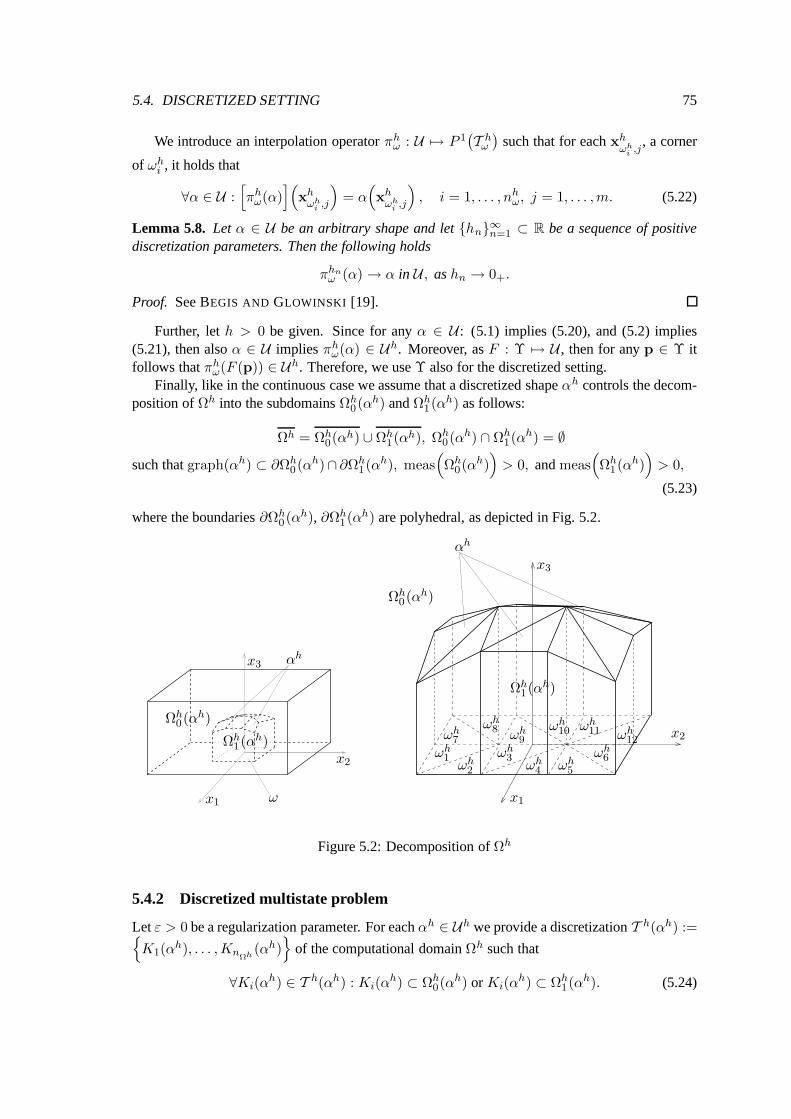
5.4. DISCRETIZED SETTING 75
We introduce an interpolation operator πhω : U 7→ P 1
(T h
ω
)such that for each xh
ωhi ,j
, a corner
of ωhi , it holds that
∀α ∈ U :[πh
ω(α)](
xhωh
i ,j
)= α
(xh
ωhi ,j
), i = 1, . . . , nh
ω, j = 1, . . . ,m. (5.22)
Lemma 5.8. Let α ∈ U be an arbitrary shape and let hn∞n=1 ⊂ R be a sequence of positivediscretization parameters. Then the following holds
πhnω (α) → α in U , as hn → 0+.
Proof. See BEGIS AND GLOWINSKI [19].
Further, let h > 0 be given. Since for any α ∈ U : (5.1) implies (5.20), and (5.2) implies(5.21), then also α ∈ U implies πh
ω(α) ∈ Uh. Moreover, as F : Υ 7→ U , then for any p ∈ Υ itfollows that πh
ω(F (p)) ∈ Uh. Therefore, we use Υ also for the discretized setting.Finally, like in the continuous case we assume that a discretized shape αh controls the decom-
position of Ωh into the subdomains Ωh0(αh) and Ωh
1(αh) as follows:
Ωh = Ωh0(αh) ∪ Ωh
1(αh), Ωh0(αh) ∩ Ωh
1(αh) = ∅such that graph(αh) ⊂ ∂Ωh
0(αh)∩ ∂Ωh1(αh), meas
(Ωh
0(αh))
> 0, and meas(Ωh
1(αh))
> 0,
(5.23)
where the boundaries ∂Ωh0(αh), ∂Ωh
1(αh) are polyhedral, as depicted in Fig. 5.2.
PSfrag replacements
Ωh0(αh)
Ωh1(αh)
αh
x1
x2
x3
ω
PSfrag replacements
Ωh0(αh)
Ωh1(αh)
αh
x1
x2
x3
ω
ωh1
ωh2
ωh3
ωh4 ωh
5
ωh6
ωh7
ωh8 ωh
9ωh
10 ωh11 ωh
12
Figure 5.2: Decomposition of Ωh
5.4.2 Discretized multistate problem
Let ε > 0 be a regularization parameter. For each αh ∈ Uh we provide a discretization T h(αh) :=K1(α
h), . . . ,KnΩh
(αh)
of the computational domain Ωh such that
∀Ki(αh) ∈ T h(αh) : Ki(α
h) ⊂ Ωh0(αh) or Ki(α
h) ⊂ Ωh1(αh). (5.24)

76 CHAPTER 5. ABSTRACT OPTIMAL SHAPE DESIGN PROBLEM
By Eh :=
e1, . . . , enΩh
we denote the corresponding set of finite elements. For any h > 0 and
αh ∈ Uh we suppose that Assumptions 4.1–4.7 hold. We introduce another assumption, which isdue to HASLINGER AND NEITTAANMAKI [85, p. 67].
Assumption 5.3. We assume that for any h > 0 fixed the topology of the discretization gridT h(αh) is independent from αh ∈ Uh, we further assume that the coordinates of x
ei
1 (αh), . . . ,x
ei
m+1(αh) ∈ Rm, see (4.25), which are the corners of Ki(α
h) ∈ T h(αh), still form a triangle(m = 2) or a tetrahedron (m = 3), and they depend continuously on αh ∈ Uh.
The regularized and discretized setting of the multistate problem reads as follows:
Find uv,hε
(αh)∈ H0
(B; Ωh
)h:
ahε,αh
(vh,uv,h
ε
(αh))
= f v,h(vh)
∀vh ∈ H0
(B; Ωh
)h
, v = 1, . . . , nv, (W v,hε (αh))
where the finite element space H0
(B; Ωh
)his defined by (4.17), where further for each vh,wh ∈
H(B; Ωh
)we define
ahε,αh
(vh,wh
):=
∫
Ωh
B(vh)·(Dh
αh · B(wh))
dx + ε
∫
Ωh
vh ·wh dx, (5.25)
in which, in virtue of Assumption 5.1,
Dhαh(x) :=
D0 , x ∈ Ωh0
(αh)
D1 , x ∈ Ωh1
(αh)
0 , x ∈ Ω \ Ωh
, (5.26)
and where for each vh ∈ H(B; Ωh
)we set
fv,h(vh)
:=
∫
Ωh
fv,h · vh dx, v = 1, . . . , nv,
in which, due to (4.18), f v,h ∈[L2(Ωh)]ν1 are elementwise constant and such that
∥∥∥fv,h − f v∥∥∥
ν1,0,Ω→ 0, as h → 0+, v = 1, . . . , nv, (5.27)
where f v,h(x) := f v(x) in Ω \ Ωh. The following is in virtue of Assumption 5.2.
Assumption 5.4. We assume that for each v = 1, . . . , nv the right–hand side f v,h is independentof the shape αh ∈ Uh.
The following lemma assures that for any ε > 0, h > 0, and v = 1, . . . , nv fixed the mapping
uv,hε : Uh 7→ H0
(B; Ωh
)his well defined.
Lemma 5.9. For each ε > 0, h > 0, αh ∈ Uh, and v = 1, . . . , nv there exists a unique solution
uv,hε
(αh)∈ H0
(B; Ωh
)hto the problem (W v,h
ε (αh)).
Proof. Since Ωh is a polyhedron, then Ωh ∈ L and the statement follows by the same argumentsas in the proof of Theorem 3.17.
5.4. DISCRETIZED SETTING 77
Lemma 5.10. Let ε > 0, h > 0. Then for each v = 1, 2, . . . , nv the mapping uv,hε : Uh 7→
H0
(B; Ωh
)his continuous on Uh.
Proof. We take an arbitrary ε > 0, h > 0, and v = 1, . . . , nv. Note that we cannot use thesame technique as in the proof of Lemma 5.3, since the settings (W v,h
ε (αh)) differ from αh ∈ Uh.Therefore, the estimate (5.11) cannot be established. We will rather exploit the algebraic structureof the mapping u
v,hε .
In the similar manner as in (4.24), the solution to (W v,hε (αh)) reads as follows:
uv,hε
(αh)
=n∑
i=1
uv,nε,i
(xh(αh))ξh
i
(xh(αh))
, (5.28)
where xh(αh)
denotes a vector of global coordinates of all element domains corners, which areby Assumption 5.3 continuously dependent on the shape αh ∈ Uh, where further ξh
i
(xh)
denotesthe global shape functions, and where we use the same notation for both the functions u
v,nε
(αh)
and uv,nε
(xh(αh))
uv,nε
(αh)≡ uv,n
ε
(xh(αh))
:=(uv,n
ε,1
(xh(αh))
, . . . , uv,nε,n
(xh(αh)))
∈ Rn,
which is the solution to the linear system (4.9). In this case, (4.9) reads as follows:
Anε
(xh)· uv,n
ε
(xh)
= f v,n(xh)
. (5.29)
Now, let us take a look into the assembling of the matrix and the right–hand side vectorin (5.29). Due to (4.21), the element contributions to them are
(An
ε
(xh))
i,j=
∑
e∈Ehi∩Eh
j
ne∑
k,l=1
aeε,xe(ξe
k(xe) , ξe
l (xe)) ,
(f v,n
(xh))
i=∑
e∈Ehi
ne∑
k=1
fv,e(ξek(x
e)) ,
(5.30)
for i, j = 1, . . . , n, where Ehi denotes the set of elements neighbouring with ei, see (4.20), and
xe is the vector of coordinates of the element domain corners, see (4.25). Using the map fromthe reference element r, the element contributions to the bilinear form and linear functional, seealso (4.29) and (4.30), respectively are
aeε,xe(ξe
k(xe) , ξe
l (xe)) =
=
∫
Kr
(Se
B(xe) · Bbx
(ξr
k
))·(De
xe ·(Se
B(xe) · Bbx
(ξr
l
)))|det(Re(xe))| dx +
+ ε
∫
Kr
(Se(xe) · ξr
k
)·(Se(xe) · ξr
l
)|det(Re(xe))| dx,
fv,e(ξek(x
e)) =
∫
Kr
f e ·(Se(xe) · ξr
k
)|det(Re(xe))| dx,
(5.31)where k, l = 1, . . . , ne and where we also used Assumptions 5.1 and 5.4.
78 CHAPTER 5. ABSTRACT OPTIMAL SHAPE DESIGN PROBLEM
The expressions (5.28)–(5.31) specify the function uv,hε
(αh). Now, we will prove its continu-
ity. Let αh ∈ Uh be an arbitrary discretized admissible shape and letαh
p
∞p=1
⊂ Uh be such asequence that
αhp → αh in Uh, as p → ∞.
Let us denote for each element e ∈ Eh, where Eh stands for the set of finite elements,
xep := xe
(αh
p
)and xe := xe
(αh)
.
By Assumption 5.3, for each element e ∈ Eh we get
xep → xe in Rm(m+1), as p → ∞.
Again by Assumption 5.3, for each e ∈ Eh and each p ∈ N the element domains Ke(xe
p
)as
well as Ke(xe) still form a triangle (in case of m = 2) or a tetrahedron (in case of m = 3), and itfollows from the definition (4.28) that the matrices Re
(xe
p
), Re(xe) are nonsingular, and therefore
∣∣det(Re(xe
p
))∣∣ > 0, |det(Re(xe))| > 0.
Moreover, as both Re and re by (4.28) continuously depend on xe, we get:
det(Re(xe
p
))→ det(Re(xe)) in R, as p → ∞. (5.32)
From Assumption 4.2 it follows that
Se(xe
p
)→ Se(xe) in Rν1×ν1 and Se
B
(xe
p
)→ Se
B(xe) in Rν2×ν2 , as p → ∞. (5.33)
Now, the only symbols in the integrals (5.31) that depend on the integration variable x are
ξrk(x), ξr
l (x), Bbx
(ξr
k(x))
, and Bbx
(ξr
l (x))
. However, they are each independent from the vector
xe. We can expand the matrix multiplications in the integrands, which leads to the following finitelinear combinations of integrals
aeε,xe(ξe
k(xe) , ξe
l (xe)) =
N∑
i=1
ceε,i(x
e)
∫
Kr
Fi(x) dx,
fv,e(ξek(x
e)) =
M∑
j=1
dv,ej (xe)
∫
Kr
Gj(x) dx.
From (5.32) and (5.33) for i = 1, . . . , N , j = 1, . . . ,M it follows that
ceε,i
(xe
p
)→ ce
ε,i(xe) and dv,e
j
(xe
p
)→ dv,e
j (xe) in R, as p → ∞,
which consequently yields
aeε,xe
p
(ξe
k
(xe
p
), ξe
l
(xe
p
))→ ae
ε,xe(ξek(x
e) , ξel (x
e)) in R, as p → ∞
andfv,e
(ξe
k
(xe
p
))→ f v,e(ξe
k(xe)) in R, as p → ∞
for k, l = 1, . . . , ne. By Assumption 5.3 the topology of the mesh T h(αh)
does not change withany αh ∈ Uh, hence, the sets Eh
i and Ehj in (5.30) remain unchanged. It follows that
(An
ε
(xh(αh
p
)))i,j
→(An
ε
(xh(αh)))
i,j, as p → ∞,
5.4. DISCRETIZED SETTING 79
and (f v,n
(xh(αh
p
)))i→(f v,n
(xh(αh)))
iin R, as p → ∞,
for each i, j = 1, . . . , n. From here and (5.29) we get
uv,nε
(xh(αh
p
))→ uv,n
ε
(xh(αh))
in Rn, as p → ∞. (5.34)
Using the map from the reference element r, the global shape function reads as follows:
ξhi
(xh)
=∑
e∈Ehi
∑
j:Ge(j)=i
ξej(x
e) =∑
e∈Ehi
∑
j:Ge(j)=i
Se(xe) · ξrj ,
which together with (5.33) and with Assumption 5.3 yield
ξhi
(xh(αh
p
))→ ξh
i
(xh(αh))
in Rn, as p → ∞. (5.35)
Combining (5.28), (5.34), and (5.35), we have completed the proof, i.e.,
uv,hε
(αh
p
)→ uv,h
ε
(αh)
in Uh, as p → ∞.
Lemma 5.11. Let ε > 0 be a regularization parameter. Let hn∞n=1 ⊂ R be a sequence ofpositive discretization parameters such that hn → 0+, as n → ∞. Let
Ωhn
∞n=1
, Ωhn ⊂ Ω, bea sequence of subdomains satisfying Ωhn Ω, as n → ∞. Further, let α ∈ U be a shape andαhn
∞n=1
⊂ U , αhn ∈ Uhn , be a sequence of discretized shapes such that
αhn → α in U , as n → ∞.
Then for each v = 1, . . . , nv
Xhnν1
(uv,hn
ε
(αhn
))→ uv
ε(α) in H0(B; Ω), as n → ∞,
where uv,hnε
(αhn
)is the solution to (W v,hn
ε (αhn)) and uvε(α) is the solution to (W v
ε (α)).
Proof. It is enough to prove that the assumption (4.42) is fulfilled and the rest is then fairly thesame as the proof of Theorem 4.2, while (4.43) is replaced by the assumption (5.27).
Given an arbitrary x ∈ Ω \ (∂Ω0(α) ∪ ∂Ω1(α)), it follows from (5.6) that either x ∈ Ω0(α)or x ∈ Ω1(α). Thus, by (5.7) either
Dα(x) = D0 or Dα(x) = D1,
respectively. Having Ωhn Ω, αhn ⇒ α, as n → ∞, and due to (5.23), there exists n0(x) ∈ N
such that for each n ∈ N, n ≥ n0(x) either x ∈ Ωhn
0
(αhn
)or x ∈ Ωhn
1
(αhn
), respectively.
Therefore, eitherDαhn (x) = D0 or Dαhn (x) = D1,
respectively. Thus, we have verified the assumption (4.42), i.e., for any i, j = 1, . . . , ν2:∣∣∣dhn
αhn ,i,j(x) − dα,i,j(x)
∣∣∣→ 0 a.e. in Ω, as n → ∞,
where Dαhn (x) :=(dhn
αhn ,i,j(x))
i,j∈ Rν2×ν2 and Dα(x) := (dα,i,j(x))i,j ∈ Rν2×ν2 .
80 CHAPTER 5. ABSTRACT OPTIMAL SHAPE DESIGN PROBLEM
5.4.3 Discretized optimization problem
The regularized and discretized cost functional is
J hε
(αh)
:= I(αh,B
(Xh
ν1
(u1,h
ε
(αh)))
, . . . ,B(Xh
ν1
(unv,h
ε
(αh))))
, αh ∈ Uh, (5.36)
where Xhν1
: H0
(B; Ωh
)h 7→ H0(B; Ω) is due to (4.33) and Lemma 4.3. The relevant setting ofthe shape optimization problem reads as follows:
Find αhε∗ ∈ Uh:
J hε
(αh
ε∗)≤ J h
ε
(αh)
∀αh ∈ Uh
. (P h
ε )
Theorem 5.5. Let ε > 0 and h > 0. Then there exists αhε∗ ∈ Uh that is a solution to (P h
ε ).
Proof. Taking any ε > 0 and h > 0, the proof is fairly the same as the one of Theorem 5.2, wherewe use the symbol J h
ε instead of J , and Lemma 5.10 instead of Lemma 5.3.
Theorem 5.6. Let ε > 0 be a fixed regularization parameter. Let hn∞n=1 ⊂ R be a sequenceof positive discretization parameters such that hn → 0+, as n → ∞, and let αhn
ε∗ ∈ Uhn denote
the corresponding solutions to the problems (P hnε ). Then there exist a subsequence hnk
∞k=1 ⊂hn∞n=1 and a shape αε
∗ ∈ U such that
αhnkε
∗→ αε
∗ in U , as k → ∞,
holds and, moreover, αε∗ is a solution to the problem (Pε).
Proof. By Theorem 5.5, for each ε > 0 and hn > 0 there exists αhnε
∗ ∈ Uhn , a solution to (P hnε ).
By Lemma 5.1, there exist a subsequence of shapesα
hnkε
∗∞
k=1⊂
αhnε
∗∞
n=1and a shape
αε∗ ∈ U such that
αhnkε
∗→ αε
∗ in U , as k → ∞. (5.37)
Let α ∈ U be an arbitrary shape. By Lemma 5.8, there exists a sequenceαhnk
∞k=1
, αhnk ∈ Uhnk
such thatαhnk → α in U , as k → ∞. (5.38)
Then, due to the definition of (Phnkε ) for any k ∈ N we have
J hnkε
(α
hnkε
∗)≤ J hnk
ε
(αhnk
). (5.39)
Using (5.37), (5.38), Lemma 5.11, and the continuity of I , both the left and right–hand sideof (5.39) converge
J hnkε
(α
hnkε
∗)→ J (αε
∗) and J hnk
(αhnk
)→ J (α) , as k → ∞.
Therefore, we have proven that for any α ∈ U
J (αε∗) ≤ J (α).
5.4. DISCRETIZED SETTING 81
Finally, we introduce the regularized and discretized cost functional J hε : Υ 7→ R by
J hε (p) := J h
ε
(πh
ω(F (p)))
, p ∈ Υ.
Then, the regularized and discretized optimization problem reads as follows:
Find phε∗ ∈ Υ:
J hε
(ph
ε∗)≤ J h
ε (p) ∀p ∈ Υ
. (P h
ε )
Since Υ is a compact set and πhωF : Υ 7→ Uh is a continuous mapping, we can state and prove the
existence theorem for (P hε ) similarly to Theorem 5.5. We can also state the convergence theorem,
the proof of which is even simpler than the one of Theorem 5.6, as the set of admissible designparameters Υ is not changed by discretization.
Remark 5.1. In cases of complex geometries, as those in Chapter 7, Assumption 5.3 is a seriousbottleneck of this discretization approach. For small discretization parameters and large changesin the design we cannot guarantee that the perturbed elements still satisfy some regularity con-dition. They might be even flipped. In this case, we have to re–mesh the geometry and solve theoptimization problem again, but now on a grid of different topology. Then certainly the cost func-tional is not continuous any more and the just introduced convergence theory cannot be applied.Nevertheless, in literature this approach is still the most frequently used one as far as a finite ele-ment discretization is concerned. In practice, after we get an optimized shape we should comparethe value of a very fine discretized cost functional for the optimized design with that value for theinitial one. If we can see a progress then the optimization surely did a good job. Some solutions tothis obstacle are discussed in Conclusion.

82 CHAPTER 5. ABSTRACT OPTIMAL SHAPE DESIGN PROBLEM
Chapter 6
Numerical methods for shapeoptimization
In this chapter, which is the heart of the thesis, we will focus on the Newton–type algorithms forsmooth discretized shape optimization problems. At the beginning, we will revise the discretizedsetting and we will show its smoothness, i.e., the continuity of both the cost and constraint func-tions up to their second derivatives. Further, we will recall a quasi–Newton algorithm that usesthe first–derivatives only. Then, we will discuss the first–order sensitivity analysis methods. Wewill derive a robust, but still efficient, algorithm based on the algebraic approach of the first–ordershape sensitivity analysis, and we will implement it into an object–oriented software framework.At the end, we will introduce a multilevel optimization approach.
An extensive literature on the gradient– or Newton–type optimization methods has been writ-ten. Let us refer to NOCEDAL AND WRIGHT [148], FLETCHER AND REEVES [63], FLET-CHER [61, 62], SVANBERG [203, 204], DENNIS AND SCHNABEL [55], GILL, MURRAY, AND
WRIGHT [66], GROSSMANN AND TERNO [72], CEA [39], CLARKE [48], HAGER, HEARN, AND
PARDALOS [81], HESTENSEN [88, 89], POLAK [161], POLAK AND RIBIERE [162], BOGGS AND
TOLLE [23], CONN, GOULD, AND TOINT [49], MAKELA AND NEITTAANMAKI [130], ZOWE,KOCVARA, AND BENDSØE [222]. There are many essential monographs and papers dealing withthe sensitivity analysis in shape optimization. Let us mention HAUG, CHOI, AND KOMKOV [86],HASLINGER AND NEITTAANMAKI [85], HASLINGER AND MAKINEN [83], ZOLESIO [220],SOKOLOWSKI AND ZOLESIO [196], SOKOLOWSKI AND ZOCHOWSKI [195], PETERSSON [157],SIMON [193], LAPORTE AND TALLEC [118], DELFOUR AND ZOLESIO [54], HANSEN, ZIU,AND OLHOFF [82], BROCKMAN [34], GRIEWANK [70], MAKINEN [131], NEITTAANMAKI AND
SALMENJOKI [145].
6.1 The discretized optimization problem revisited
Throughout this chapter, we will consider the optimization problem (P hε ), introduced in Chapter 5.
Recall that for a given ε > 0 and h > 0 the problem reads as follows:
Find phε∗ ∈ Υ:
J hε
(ph
ε∗)≤ J h
ε (p) ∀p ∈ Υ
, (P h
ε )
where J hε : Υ 7→ R denotes the discretized and regularized cost functional and Υ ⊂ RnΥ ,
nΥ ∈ N, is the set of admissible design parameters.
83
84 CHAPTER 6. NUMERICAL METHODS FOR SHAPE OPTIMIZATION
6.1.1 Constraint function
Let us rewrite the admissible set as follows:
Υ := p ∈ RnΥ | υ(p) ≤ 0 ,
where υ : RnΥ 7→ Rnυ , nυ ∈ N, is the constraint function.
Assumption 6.1. We assume that υ ∈[C2(RnΥ)
]nυ .
6.1.2 Design–to–shape mapping
Let us take a deep look into the structure of the cost functional in order to prove its smoothnessand to derive the first–order derivatives with respect to the design variables. First, we define the
shape parameterization function αh :=(αh
1 , . . . , αhn
αh
): RnΥ 7→ Rn
αh , nαh := nxhω∈ N, by
αhi (p) :=
(πh
ω F)
(p) ≡ [F (p)](xh
ω,i
)for i = 1, . . . , nαh , (6.1)
where F : Υ 7→ U is due to (5.5) and πhω : U 7→ P 1
(T h
ω
)is defined by (5.22).
6.1.3 Shape–to–mesh mapping
Here, we revisit the dependence of the discretization grid nodes on the shape control nodes, i.e., weintroduce a function xh : Rn
αh 7→ Rmnx
h the components of which correspond to the grid nodalcoordinates (4.11), where nxh ∈ N denotes the number of nodes in the discretization T h(αh) ofthe domain Ωh. The function xh(·) maps the control shape coordinates onto the remaining gridnodal coordinates by means of solving an auxiliary discretized linear elasticity problem in terms ofgrid displacements 4xh with a nonhomogeneous Dirichlet boundary condition that correspondsto given shape displacements αh, and with prescribed zero displacements on ∂Ωh and on suchinner interfaces that are not allowed to move. The zero displacements are, for example, prescribedalong the boundary of a subdomain containing nonzero sources f h. The shape–to–mesh mappingis as follows:
xh(αh)
:= xh0 + 4xh
(αh)
+ Mh · αh, where K h(xh
0
)· 4xh
(αh)
= bh(αh)
, (6.2)
in which the vector xh0 ∈ Rmn
xh contains the initial grid nodal coordinates and is independent
of αh, where further K h(xh
0
)∈ R(mn
xh)×(mn
xh) is a nonsingular symmetric stiffness matrix,
bh(αh)∈ Rmn
xh is a right–hand side vector linearly dependent onαh ∈ Rn
αh , and where finally
Mh ∈ R(mnx
h)×nαh is a rectangular permutation matrix that identically maps the shape nodal
coordinates onto the corresponding grid nodal coordinates. Both K h and bh arise from the finiteelement discretization of the auxiliary linear elasticity problem. For finite elements in elasticity, werefer to ZIENKIEWICZ [217]. The matrix Mh might also involve some symmetry assumptions onthe geometry, as we will state later in Chapter 7. Solving the equation (6.2) takes approximatelythe same computational effort as solving one state problem. Nevertheless, the mapping is verygeneral, which fits to our intent in developing a robust and efficient numerical method for shapeoptimization.

6.1. THE DISCRETIZED OPTIMIZATION PROBLEM REVISITED 85
6.1.4 Multistate problem
Concerning the multistate problem, we recall that we arrive at solving the following nv linearsystems of algebraic equations
Anε
(xh)· uv,n
ε
(xh)
= f v,n(xh)
, v = 1, . . . , nv, (6.3)
where both the system matrix and the right-hand side vectors are assembled by means of Algo-rithm 1 (
Anε
(xh))
i,j:=
∑
e∈Ehi ∩Eh
j
ne∑
k,l=1
aeε,xe(ξe
k(xe) , ξe
l (xe)) ,
(f v,n
(xh))
i:=∑
e∈Ehi
ne∑
k=1
fv,e(ξek(x
e))
(6.4)
for i, j = 1, . . . , n, where Ehi denotes the set of elements neighbouring with ei, see (4.20), and
xe ∈ Rm(m+1) is the vector of coordinates of the element domain corners, see (4.25), which isalso included in xh by means of the mapping He, see (4.26). Components of the solution to (6.3)are denoted by
uv,nε :=
(uv,n
ε,1 , . . . , uv,nε,n
)∈ Rn, v = 1, . . . , nv.
Using the map from the reference element r, the element contributions to the bilinear form andlinear functional, respectively, see also (4.29) and (4.30), are
aeε,xe(ξe
k(xe) , ξe
l (xe)) :=
:=
∫
Kr
(Se
B(xe) · Bbx
(ξr
k(x)))
·(De ·
(Se
B(xe) ·Bbx
(ξr
l (x))))
|det(Re(xe))| dx +
+ ε
∫
Kr
(Se(xe) · ξr
k(x))·(Se(xe) · ξr
l (x))|det(Re(xe))| dx,
fv,e(ξek(x
e)) :=
∫
Kr
fv,e ·(Se(xe) · ξr
k(x))|det(Re(xe))| dx,
(6.5)where k, l = 1, . . . , ne and where we consider (5.26) and Assumption 5.4. Then,
uv,hε
(xh;x
)=
n∑
i=1
uv,nε,i
(xh)ξh
i
(xh;x
), v = 1, . . . , nv, xh ∈ Rmn
xh , x ∈ Ωh, (6.6)
is the solution to the state problem (W v,hε (αh)), where ξh
i
(xh;x
)denote the global shape func-
tions. Moreover, for e ∈ Eh we introduce the element solution vector by
uv,n,eε :=
(uv,n,e
ε,1 , . . . , uv,n,eε,ne
)∈ Rne , where uv,n,e
ε,i := uv,nε,Ge(i) for i = 1, . . . , ne.
As we look for B(u
v,hε
)rather than for u
v,hε , we further elementwise evaluate the following
block column vector
Bv,nε
(xh)
:=[Bv,n,e1
ε
(xh)
, . . . ,Bv,n,en
Ωh
ε
(xh)]
:= B(xh,u v,n
ε
(xh))
∈ Rν2nΩh (6.7)
86 CHAPTER 6. NUMERICAL METHODS FOR SHAPE OPTIMIZATION
for v = 1, . . . , nv, where for i = 1, . . . , nΩh the corresponding element vector is defined by
Bv,n,eiε
(xh)
:= B(xei ,uv,n,ei
ε
(xh))
,
and where xh ∈ Rmnx
h contains all the grid nodes, xe ∈ Rmne contains the grid nodes related tothe element e ∈ Eh, where further
B(xh,uv,n
ε
(xh))
|Ki:= B
(xei ,u v,n,ei
ε
(xh))
:= Bx
(uv,h
ε
(xh;x
))|Ki
=
=
ne∑
j=1
uv,nε,Gei(j)(x
ei)Bx
(ξei
j (xei ;x))
=
=
ne∑
j=1
uv,n,ei
ε,j (xei)Sei
B(xei) ·Bbx
(ξr
j(x))
for i = 1, . . . , nΩh ,
(6.8)
where x := Rei ·x+rei ∈ Ki, and where ei ∈ Eh is the element related to Ki. Recall that since we
employ the lowest, i.e., first–order finite elements, the function Bx
(u
v,hε (xh;x)
)is elementwise
constant.
6.1.5 Cost functional
Now, we revisit the cost functional (5.36) from the algebraic point of view. In addition, it dependson the vector of grid nodal coordinates xh as follows:
J hε (p) := Ih
(αh(p),xh
(αh)
,B1,nε
(xh)
, . . . ,Bnv,nε
(xh))
,
whereαh := αh(p) is a vector of shape control coordinates, where for v = 1, . . . , nv Bv,nε
(xh)∈
Rν2nΩh is given by (6.7) and (6.8), and where Ih : Rn
αh ×Rmnx
h ×[Rν2nΩh ]nv 7→ R is the revised
cost functional which is for p ∈ Υ and for xh := xh(αh(p)
)defined by
Ih(αh(p),xh,B1,n
ε
(xh)
, . . . ,Bnv,nε
(xh))
:=
:= I(πh
ω(F (p)) ,Xhν1
(B(u1,h
ε
)), . . . ,Xh
ν1
(B(unv,h
ε
))),
in which πhω : U 7→ Uh is defined by (5.22), F : Υ 7→ U is due to (5.5), Xh
ν1: H0
(B; Ωh
)7→
H0(B; Ω) is due to (4.33) and Lemma 4.3, and where uv,hε is the solution (6.6).
The complete evaluation of the cost functional proceeds as follows:
pπh
ωF−−−−→ αhKh·4xh=bh(α
h)−−−−−−−−−−−→ xh FEM−−−−→ Anε , f v,n An
ε ·uv,nε =f v,n
−−−−−−−−−→ uv,nε
B(xh,uv,nε )−−−−−−−→
B(xh,uv,nε )−−−−−−−→ Bv,n
ε
Ih(αh,xh,B1,nε ,...,Bnv,n
ε )−−−−−−−−−−−−−−−−→ J hε (p).
(6.9)The cost functional J h
ε is compounded of the following submappings:
• αh which is the discretized shape parameterization,
• K h · 4xh = bh(αh), see (6.2), that maps the shape control nodal coordinates αh onto the
remaining nodal coordinates xh in the grid,
6.1. THE DISCRETIZED OPTIMIZATION PROBLEM REVISITED 87
• FEM which assembles the system matrix Anε and the right–hand side vectors f 1,n, . . . ,
f nv,n by means of the finite element method, as described in Algorithm 1,
• Anε · uv,n
ε = f v,n that solve the nv linear systems of algebraic equations,
• Bv,nε which is a block column vector whose individual vectors represent the elementwise
constant functions Bx
(u
v,hε (x)
), see in Algorithm 2, and
• Ih which calculates the cost functional.
6.1.6 Smoothness of the cost functional
To prove the smoothness of J hε , we need the smoothness of all the submappings.
Assumption 6.2. We assume that for each h > 0 such that h ≤ h the following hold:
• ∀x ∈ ω : [F (·)] (x) ∈ C2(Υ) ,
• K h ∈ R(mnx
h)×(mnx
h) is nonsingular,
• bh(αh)∈[C2(Rn
αh )]mn
xh ,
• ∀e ∈ Eh : Re(xe) ∈[C2(Rm(m+1)
)]m×m,
• ∀e ∈ Eh : SeB(xe) ∈
[C2(Rm(m+1)
)]ν2×ν2 ,
• ∀e ∈ Eh : Se(xe) ∈[C2(Rm(m+1)
)]ν1×ν1 , and
• Ih(αh,B1,n
ε , . . . ,Bnv,nε
)∈ C2(Rn
αh × (Rν2nΩh )nv) .
Lemma 6.1. Under Assumptions 5.1, 5.3, 5.4, and 6.2, for any h > 0 such that h ≤ h it holdsthat
J hε ∈ C2(Υ).
Proof. We will step–by–step use Assumption 6.2 and apply Lemma 3.4 to prove the smoothnessof the individual submappings.
Let h > 0 be given such that h ≤ h. By Assumption 6.2, for each i = 1, . . . , nxhω
we have
[F (·)](xh
ω,i
)∈ C2(Υ), therefore,
αh ∈(C2(Υ)
)nαh . (6.10)
Again by Assumption 6.2 and by Lemma 3.3, det(K h)6= 0 and
[K h]−1
:=1
det(K h)Kh,
holds, where K h denotes the adjoint matrix, which was defined by (3.13). Then, due to the latterand by Assumption 6.2, we get
xh(αh)
=[K h]−1
· bh(αh)∈[C2(Rn
αh )]mn
xh . (6.11)
88 CHAPTER 6. NUMERICAL METHODS FOR SHAPE OPTIMIZATION
Now, (6.10), (6.11), and Lemma 3.4 yield
xh αh ∈[C2(Υ)
]mnx
h .
Let us further prove the smoothness of the solutions uv,nε
(xh)
to the discretized multistateproblem (6.3). Let ε > 0 and v = 1, . . . , nv be arbitrary. By Assumption 6.2, for each e ∈ Eh weget
Re ∈[C2(Rm(m+1)
)]m×m, Se
B ∈[C2(
Rm(m+1))]ν2×ν2
, Se ∈[C2(Rm(m+1)
)]ν1×ν1
.
Then, also due to the definition (3.12), det(Re) ∈ C2(Rm(m+1)
). From Assumption 5.3 it follows
that the element Ke must not flip, so the determinant does not change its sign, i.e.,
|det(Re)| ∈ C2(
Rm(m+1))
.
Now let us look at the element contributions (6.5). Having Assumptions 5.1 and 5.4, only the ref-erence shape functions ξr
k and ξrl depend on the integration variable x. After some matrix–vector
multiplications we get the following structure of the element bilinear form and linear functional,respectively,
aeε,xe(ξe
k(xe) , ξe
l (xe)) =
N∑
i=1
ceε,i(x
e)
∫
Kr
Fi(x) dx,
fv,e(ξek(x
e)) =M∑
i=1
dv,ei (xe)
∫
Kr
Gi(x) dx,
where both ceε,i(x
e) , dv,ei (xe) ∈ C2
(Rm(m+1)
), since they arise as sumations and multiplications
of the entries of SeB, De, Se, and f v,e multiplied then by |det(Re)|, and where both Fi(x) and
Gi(x) are common for all e ∈ Eh. Thus, it follows that both the element bilinear form and elementlinear functional are smooth, i.e.,
aeε,xe(ξe
k(xe) , ξe
l (xe)) ∈
[C2(Rm(m+1)
)]ne×ne
, fv,e(ξek(x
e)) ∈[C2(Rm(m+1)
)]ne
. (6.12)
Now we employ Assumption 5.3, which assures that the topology of the discretization T h is fixed.Hence, neither Eh
i nor Ehj in (6.3) depends on xh. From (6.12) it follows that
Anε
(xh)∈[C2(Rmn
xh )]n×n
and f v,n(xh)∈[C2(Rmn
xh )]n
,
a consequence of which is
det(An
ε
(xh))
∈ C2(Rmnx
h ) .
Lemma 5.9 provides us the existence of the solution uv,nε
(xh)
to (6.3). Hence, there exist the
inverse matrix[An
ε
(xh)]−1
. Then, by Lemma 3.3, det(An
ε
(xh))
6= 0 and
[An
ε
(xh)]−1
:=1
det(Anε (xh))
Anε
(xh)∈[C2(Rmn
xh )]n×n
holds, where Anε
(xh)
denotes the adjoint matrix, which was defined by (3.13). From (3.15) weget
uv,nε
(xh)
=[An
ε
(xh)]−1
· f v,n(xh)∈[C2(Rmn
xh )]n
for v = 1, . . . , nv. (6.13)
6.2. NEWTON–TYPE OPTIMIZATION METHODS 89
The symbol Bv,nε is calculated by (6.7) and (6.8). Since there appear only summations and mul-
tiplications of the components of uv,n,eε
(xh)
and SeB(xe) with the constant vectors Bbx
(ξr
j(x))
,
we can use (6.13) and Lemma 3.4 which yield
Bv,nε
(xh)
:= B(xh,u v,n
(xh))
∈[C2(Rmn
xh )]ν2n
Ωh for v = 1, . . . , nv. (6.14)
Finally, we compound the submappings αh : Υ 7→ Rnαh , xh : Rn
αh 7→ Rmnx
h , Bv,nε :
Rmnx
h 7→ Rν2nΩh , and Ih : Rnα × Rmn
xh × (Rν2n
Ωh )nv 7→ R. First, Assumption 6.2 yields
Ih ∈ C2(Rnαh × Rmn
xh × (Rν2n
Ωh )nv) .
Then, using the latter, (6.10), (6.14), and applying Lemma 3.4, we have proven the statement
J hε := Ih
[αh ×
(xh αh
)×(B1,n
ε xh αh)× · · · ×
(Bnv,n
ε xh αh)]
∈ C2(Υ).
Convention 6.1. Just for the purposes of this chapter let us skip in our notation the discretizationparameter h, the superscript n in (6.3), and the regularization parameter ε that will be eachfixed for the moment. If not stated otherwise, all the symbols in the sequel will be consideredas discretized ones, even if they were previously reserved for the continuous setting. Hence, weconsider the following discrete optimization problem with inequality constraints
Find p∗ := arg minp∈R
nΥ
J (p)
subject to υ(p) ≤ 0
, (P)
where J : RnΥ 7→ R and υ(p) := (υ1(p), . . . , υnυ (p)) : RnΥ 7→ Rnυ . The problem (P) isgoverned by the following multistate problem
A(x) · uv(x) = f v(x) (P v(x))
for v = 1, . . . , nv.
6.2 Newton–type optimization methods
Since we do not usually have any rigorous analysis locating the global solution p∗, it is hardlypossible to solve the problem (P) in a suitable computational time and with a suitable precision atthe same time, when having only some ten design variables. The algorithms looking for a globalminimizer are of an exponential order of complexity with respect to the number nΥ of designvariables. On the other hand, the Newton–type algorithms search for a local minimizer only, butthe computational time is quadratically proportional to the distance of the initial design from theclosest local minimizer. This is due to the fact that we can precisely provide derivatives of thecost function J as well as of the constraint function υ with respect to the design variables p.Here, we will restrict ourselves to developing efficient methods that calculate derivatives for shapeoptimization. We refer to NOCEDAL AND WRIGHT [148] for a detail overview of optimizationmethods for a large variety of problems.

90 CHAPTER 6. NUMERICAL METHODS FOR SHAPE OPTIMIZATION
6.2.1 Quadratic programming subproblem
The Newton–type algorithms are based on an approximation of the original nonlinear optimiza-tion problem by a quadratic or a sequence of quadratic optimization subproblems, which are alsoreferred to as quadratic programming subproblems. In general, a quadratic programming problemreads as follows:
Find p∗ := arg minp∈R
nΥ
Q(p)
subject to L(p) ≤ 0
, (QP)
where Q : RnΥ 7→ R denotes a quadratic function and L : RnΥ 7→ Rnυ denotes a linear vectorfunction.
Basically, there are two approaches to the approximation of the problem (P) by a subproblem(QP). In both of them the input p0 ∈ RnΥ denotes initial design parameters. The first approachis called a line search approach where we look for an optimal Newton direction s∗QP being thesolution to the following subproblem
Find s∗QP := arg mins∈R
nΥ
[Q(J ,p0
)](s)
subject to [L (υ,p0)] (s) ≤ 0
, (QP1(p0))
where s := p − p0 stands for a directional vector from the initial design p0 to the current one
p, Q(J ,p0
)stands for quadratic Taylor’s expansion, see Theorem 3.3, of the function J at the
point p0 while skipping the constant term J (p0)
[Q(J ,p0
)](s) := grad
(J (p0)
)· s +
1
2s ·(Hess
(J (p0)
)· s)
, s ∈ RnΥ, (6.15)
in which Hess(J (p0)
)∈ RnΥ×nΥ denotes the Hessian matrix whose entries are as follows:
[Hess
(J (p0)
)]i,j
:=∂2J (p0)
∂pi∂pj, i, j = 1, . . . , nΥ,
and where L
(J ,p0
)denotes linear Taylor’s expansion, see Theorem 3.3, of the vector function
υ at the point p0
[L(υ,p0)] (s) := υ(p0) + Grad(υ(p0)) · s, s ∈ RnΥ, (6.16)
in which the matrix Grad(υ(p0)) ∈ RnΥ×nυ denotes the following gradient matrix
Grad(υ(p0)) := [grad(υ1(p0)) , . . . ,grad(υnυ(p0))] .
The optimal direction s∗QP is then an input to the following one–dimensional optimization prob-lem, the line search problem
Find α∗QP := arg min
α>0
J(p0 + α s∗QP
)
subject to υ(p0 + α s∗QP
)≤ 0
, (LS(p0, s
∗QP))
andp∗
QP := p0 + α∗QP s∗QP
6.2. NEWTON–TYPE OPTIMIZATION METHODS 91
is the solution.The second approach is called a trust region method. It supposes that the quadratic subproblem
approximates the original problem well, but just in a given neighbourhood of p0. Hence, given aninitial point p0 and a trust region diameter d > 0, we solve the following quadratic subproblem
Find p∗QP := arg min
p∈RnΥ
[Q(J ,p0
)](p− p0)
subject to [L (υ,p0)] (p − p0) ≤ 0
‖p − p0‖ ≤ d
2
, (QP2(p0, d))
where Q and L are respectively given by (6.15) and (6.16).
6.2.2 Sequential quadratic programming
The problem (QP) is usually solved sequentially such that the optimal solution p∗QP is used as
an initial design for the next quadratic subproblem. This is also referred to as sequential quadraticprogramming (SQP). Its two simplest versions that use the line search or the trust region approach,respectively, are sketched in Algorithm 3 or in Algorithm 4, cf. NOCEDAL AND WRIGHT [148,p. 532].
Algorithm 3 Sequential quadratic programming using the line search methodGiven p0
k := 0while a convergence test is not satisfied do
Solve (QP1(pk)) s∗QP
Solve (LS(pk, s∗QP)) α∗
QP
p∗QP := p0 + α∗
QP s∗QP
pk+1 := p∗QP
k := k + 1end whilep∗ := pk
Algorithm 4 Sequential quadratic programming using the trust region methodGiven p0 and d0 > 0k := 0while a convergence test is not satisfied do
Solve (QP2(pk, dk)) p∗QP
pk+1 := p∗QP
Update dk dk+1
k := k + 1end whilep∗ := pk
Let us note that there are many aspects to deal with, as to find a proper convergence criterionor to modify the quadratic subproblem when it does not admit a solution, which is the case ifthe Hessian matrix or its certain invariant is not positive definite. Here, we want to mention the
92 CHAPTER 6. NUMERICAL METHODS FOR SHAPE OPTIMIZATION
BFGS modification, see FLETCHER [62], named after its authors Broyden, Fletcher, Goldfarb, andShanno. It is originally based on the idea of DAVIDON [52, 53]. The method was a revolutionaryimprovement of the SQP algorithm. At each iteration, it requires to evaluate only the gradient ofthe objective and constraint functions, while the Hessian matrix is iteratively built up by measuringchanges in the gradients. For k ≥ 0, k ∈ N, the BFGS formula is the following, cf. NOCEDAL
AND WRIGHT [148, p. 25],
Hk+1 := Hk −(Hk · sk) · (Hk · sk)
sk · (Hk · sk)+
yk · yTk
yk · sk, (6.17)
where Hk and Hk+1 are two successive approximations of the Hessian matrices Hess(J (pk)
)
and Hess(J (pk+1)
), respectively, and where
sk := pk+1 − pk and yk := grad(J (pk+1)
)− grad
(J (pk)
).
The SQP method with the BFGS update is classified as a quasi–Newton method.
6.3 The first–order sensitivity analysis methods
Recall that by the first–order sensitivity analysis we mean calculation of gradients of the cost andconstraint functions. There are three kinds of the sensitivity analysis methods, namely, a numericaldifferentiation, an automatic differentiation, and semianalytical methods, while others are certainmodifications and/or combinations of them.
The most frequently used is the numerical differentiation. It is usually based on formu-las for the central difference. Given a function f ∈ C 1
(Ω), Ω ⊂ Rn, and a point x :=
(x1, . . . , xi, . . . , xn) ∈ Ω, then, using linear Taylor’s expansion, see Theorem 3.3, we can de-rive the following first central difference formula
∂f(x)
∂xi≈ f(x1, . . . , xi + δ, . . . , xn) − f(x1, . . . , xi − δ, . . . , xn)
2δ,
where δ > 0. The approximation error decreases with δ2 until a computer round–off error becomessignificant. Therefore, we have to choose δ such that neither the approximation nor round–off erroris large. Another possibility is using a numerical differentiation formula of a higher m–th order,m ∈ N, for which the approximation error decreases with δm+1. However, evaluating the gradientapproximation needs 2mn evaluations of f , which is in the case of shape optimization very timeconsuming. Hence, we have to balance between the time issue and the precision. The advantagesof the method are robustness and easy implementation.
The automatic differentiation, see GRIEWANK [70], differentiate the function f symbolically.The input of the method is a routine that evaluates f(x) and the output is again a routine whichnow evaluates grad(f(x)). An implementation of the method is very difficult, since it involves asyntax recognizing, and it relies on the programming language that f is coded in. Nowadays, thereare free software packages available. The method is robust and precise up to the computer round–off error, but it is too much both time and memory consuming in case of shape optimization, sincethe routine for solving the linear system which arises from the finite element discretization is alsodifferentiated symbolically.
6.3. THE FIRST–ORDER SENSITIVITY ANALYSIS METHODS 93
Here, we will focus on the semianalytical methods, cf. HAUG, CHOI, AND KOMKOV [86],that bases on the algebraic approach to sensitivity analysis, cf. HASLINGER AND NEITTAANM A-KI [85]. The methods respect the structure of the shape optimization problem, in which solutionto a linear system of algebraic equations is involved. The cost functional is a compound map andits gradient is then a product of the gradients of the individual submappings. Most difficult toevaluate is differentiation of the solution to the linear system with respect to nodal coordinatesof the discretization grid. This is performed by solution to other linear systems with the originalbut transposed system matrix and with new right–hand side vectors. The method is precise upto the numerical error of the linear system solver. The computational time roughly correspondsto the computation of the function f . The method is not robust, as it covers just the shape opti-mization problems, nevertheless, some other classes of optimization problems, e.g., the topologyoptimization, have a similar structure. Thus, an extension of the method is straightforward. Thesemianalytical methods might also be combined with both the numerical and automatic differen-tiation.
6.3.1 Sensitivities of the cost and constraint functions
Consider the discretized shape optimization problem (P). The key point to an efficient imple-mentation of the method is making use of the structure of the cost function J . Recall that ourconstraint function is state–independent, i.e., it does not depend upon the solution to the govern-ing state problem. Therefore, the evaluation of the gradient of the constraint function with respectto the design variables is simple. For i = 1, . . . , nυ and j = 1, . . . , nΥ the gradient is as follows:
grad(υi(p)) :=
(∂υi(p)
∂p1, . . . ,
∂υi(p)
∂pnΥ
)∈ RnΥ, (6.18)
where p := (p1, . . . , pnΥ) ∈ RnΥ stands for a vector of design variables and where the constraint
function is denoted by υ(p) := (υ1(p), . . . , υnυ(p)) ∈ Rnυ . The evaluation of the cost functional
proceeds as depicted in (6.9). Let us express a partial derivative of the cost functional with respectto a design variable. Using the chain rule (3.17) for differentiation of a compound function, fori = 1, . . . , nΥ we get
∂J (p)
∂pi=
∂I(α,x,B1, . . . ,Bnv
)
∂pi=
=
nα∑
o=1
∂I(α,x,B1, . . . ,Bnv
)
∂αj+
nx∑
k=1
m∑
l=1
[∂I(α,x,B1, . . . ,Bnv
)
∂xk,l+
+
nv∑
v=1
∑
e∈E
ν2∑
j=1
∂I(α,B1, . . . ,Bnv
)
∂Bv,ej
(∂Bv,e
j (xe,uv,e)
∂xk,l+
+
ne∑
p=1
∂Bv,ej (xe,u v,e)
∂uv,ep
∂uv,ep (x)
∂xk,l
nα∑
o=1
∂xk,l(α)
∂αo
∂αo(p)
∂pi,
(6.19)
where
• p := (p1, . . . , pnΥ) ∈ RnΥ denotes a design vector,
• α(p) := (α1(p), . . . , αnα(p)) ∈ Rnα denotes control coordinates of the shape and for
o = 1, . . . , nα, i = 1, . . . , nΥ it holds that
∂αo(p)
∂pi=
∂ [F (p)](xω,o)
∂pi,
94 CHAPTER 6. NUMERICAL METHODS FOR SHAPE OPTIMIZATION
• x(α) := [x1(α), . . . ,xnx(α)] ∈ Rmnx denotes a block column vector consisting of all the
grid nodes, where for o = 1, . . . , nα
∂x(α)
∂αo:=
∂4x(α)
∂αo+
[M]1,o...
[M]nx,o
, where K (x0) ·
∂4x(α)
∂αo=
∂b(α)
∂αo,
• xe(α) :=[xe
1(α), . . . ,xem+1(α)
]∈ Rm(m+1) denotes a block column vector consisting of
the corners of the element domain Ke, e ∈ E,
• xel (α) :=
(xe
l,1(α), . . . , xel,m(α)
)∈ Rm denotes coordinates of the l–th corner of the
element domain Ke, e ∈ E,
• uv(x) := (uv1(x), . . . , uv
n(x)) ∈ Rn denotes the solution to v–th state problem, i.e., to thesystem of linear algebraic equations (P v(x)),
• uv,e(x) := (uv,e1 (x), . . . , uv,e
ne(x)) ∈ Rne denotes the solution of the problem (P v(x))
associated to an element e ∈ E in such a way that
uv,ej (x) = uv
Ge(j)(x),
• Bv(x) := [Bv,e1(x), . . . ,B v,enΩ (x)] ∈ Rν2nΩ denotes a block column vector resultingafter the application of the operator B to the solution of the problem (P v(x)),
• Bv,e(x) := (Bv,e1 (x), . . . , Bv,e
ν2(x)) ∈ Rν2 denotes the value of B(uv(x)) over the element
domain Ke, e ∈ E, such that
Bv,e(x) := B(xe,u v,e) :=
ne∑
j=1
uv,ej (x)Se
B(xe) · Bbx
(ξr
j(x))
,
and
• J (p) := I(α,x,B1, . . . ,Bnv
)∈ R denotes the value of the cost functional.
6.3.2 State sensitivity
The main computational effort in the formula (6.19) is connected with the bracket term, which isthe sensitivity of B(x,u v(x)) with respect to the grid nodal coordinates x, i.e., with the deriva-tives
∂Bv,ej (xe,uv,e(x))
∂xk,l:=
∂Bv,ej (xe,uv,e)
∂xk,l+
ne∑
p=1
∂Bv,ej (xe,uv,e)
∂uv,ep
∂uv,ep (x)
∂xk,l, (6.20)
where for k = 1, . . . , nx, l = 1, . . . ,m, and for p = 1, . . . , ne
∂Bv,ej (xe,uv,e)
∂xk,l:= 0, if ∀z ∈ 1, . . . ,m + 1 : He(z) 6= k,
∂Bv,ej (xe,uv,e)
∂xk,l:=
ne∑
p=1
uv,ep (x)
[∂Se
B(xe)
∂xez,l
· Bbx
(ξr
p(x))]
j
, if He(z) = k,
∂Bv,ej (xe,uv,e)
∂uv,ep
:=[Se
B(xe) · Bbx
(ξr
p(x))]
j.
6.3. THE FIRST–ORDER SENSITIVITY ANALYSIS METHODS 95
In (6.20) it remains to express the derivative ∂u v(x)/∂xk,l. To this goal, let us differentiate thestate equation (P v(x)), where v = 1, . . . , nv, with respect to the l–th coordinate of a node xk ∈ Ω,where k = 1, . . . , nx. We arrive at the following linear system of equations
A(x) · ∂uv(x)
∂xk,l=
∂f v(x)
∂xk,l− ∂A(x)
∂xk,l· uv(x) (6.21)
which is solved for ∂u v(x)/∂xk,l, where
∂A(x)
∂xk,l:=
∂A1,1(x)∂xk,l
. . .∂A1,n(x)
∂xk,l
.... . .
...∂An,1(x)
∂xk,l. . .
∂An,n(x)∂xk,l
,
∂f v(x)
∂xk,l:=
∂fv1(x)
∂xk,l
...∂fv
n(x)∂xk,l
,
∂u v(x)
∂xk,l:=
∂uv1(x)
∂xk,l
...∂uv
n(x)∂xk,l
,
and where A(x) := (Ai,j(x))ni,j=1, f v(x) := (f v
i (x))ni=1, and uv(x) := (uv
i (x))ni=1, respec-
tively, are the system matrix, the right–hand side vector, and the solution to the state problem(P v(x)). Due to Assumption 5.4, we can skip the term ∂f v(x)/∂xk,l. Hence, it remains toexpress the term ∂A(x)/∂xk,l. From (6.4) and (6.5) it follows that
∂Ai,j(x)
∂xk,l=
∑
e∈Ei∩Ej
ne∑
o,p=1
∂aexe
(ξe
o(xe) , ξe
p(xe))
∂xk,l,
where
∂aexe
(ξe
o(xe) , ξe
p(xe))
∂xk,l= 0, if ∀z ∈ 1, . . . ,m + 1 : He(z) 6= k,
∂aexe
(ξe
o(xe) , ξe
p(xe))
∂xk,l=
=
∫
Kr
(∂Se
B(xe)
∂xez,l
·Bbx
(ξr
o
))·(De ·
(Se
B(xe) ·Bbx
(ξr
p
)))|det(Re(xe))| dx +
+
∫
Kr
(Se
B(xe) ·Bbx
(ξr
o
))·(
De ·(
∂SeB(xe)
∂xez,l
· Bbx
(ξr
p
)))|det(Re(xe))| dx +
+
∫
Kr
(Se
B(xe) ·Bbx
(ξr
o
))·(De ·
(Se
B(xe) ·Bbx
(ξr
p
))) ∂ |det(Re(xe))|∂xe
z,l
dx +
+ ε
∫
Kr
(∂Se(xe)
∂xez,l
· ξro
)·(Se(xe) · ξr
p
)|det(Re(xe))| dx +
+ ε
∫
Kr
(Se(xe) · ξr
o
)·(
∂Se(xe)
∂xez,l
· ξrp
)|det(Re(xe))| dx +
+ ε
∫
Kr
(Se(xe) · ξr
o
)·(Se(xe) · ξr
p
) ∂ |det(Re(xe))|∂xe
z,l
dx, if He(z) = k.
(6.22)
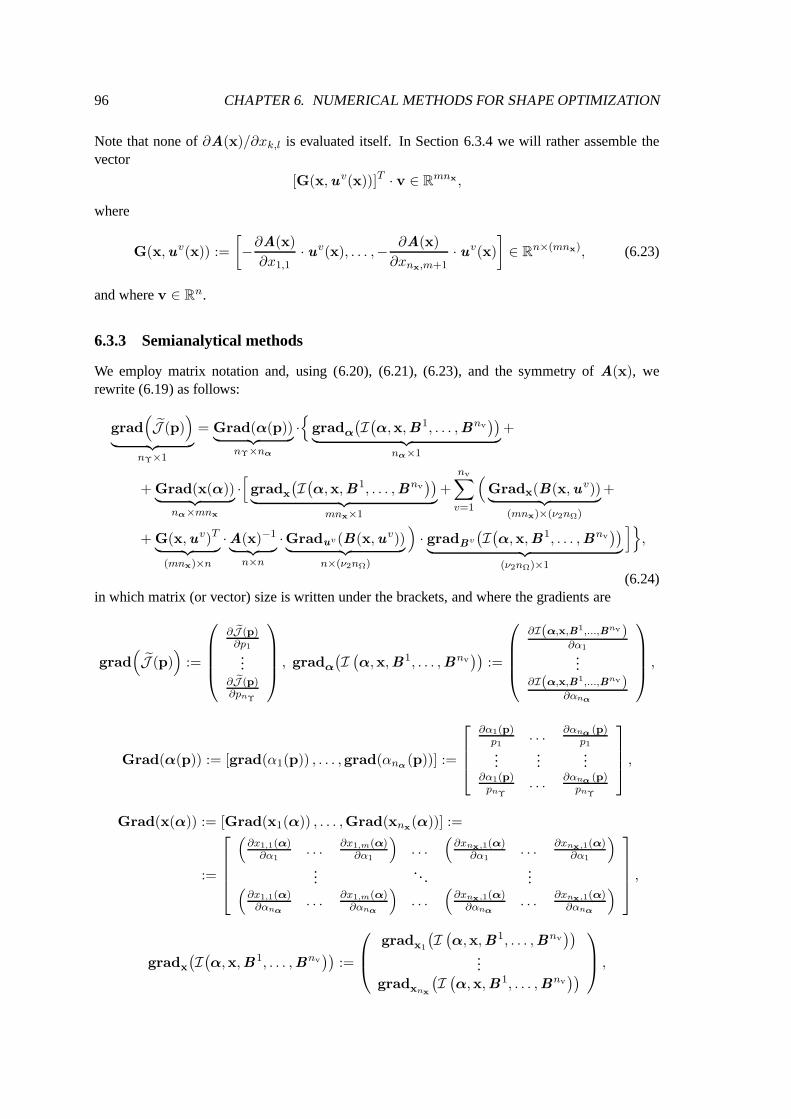
96 CHAPTER 6. NUMERICAL METHODS FOR SHAPE OPTIMIZATION
Note that none of ∂A(x)/∂xk,l is evaluated itself. In Section 6.3.4 we will rather assemble thevector
[G(x,u v(x))]T · v ∈ Rmnx ,
where
G(x,uv(x)) :=
[−∂A(x)
∂x1,1· uv(x), . . . ,− ∂A(x)
∂xnx,m+1· uv(x)
]∈ Rn×(mnx), (6.23)
and where v ∈ Rn.
6.3.3 Semianalytical methods
We employ matrix notation and, using (6.20), (6.21), (6.23), and the symmetry of A(x), werewrite (6.19) as follows:
grad(J (p)
)
︸ ︷︷ ︸nΥ×1
= Grad(α(p))︸ ︷︷ ︸nΥ×nα
·
gradα
(I(α,x,B1, . . . ,Bnv
))︸ ︷︷ ︸
nα×1
+
+ Grad(x(α))︸ ︷︷ ︸nα×mnx
·[gradx
(I(α,x,B1, . . . ,Bnv
))︸ ︷︷ ︸
mnx×1
+
nv∑
v=1
(Gradx(B(x,u v))︸ ︷︷ ︸
(mnx)×(ν2nΩ)
+
+ G(x,uv)T
︸ ︷︷ ︸(mnx)×n
·A(x)−1
︸ ︷︷ ︸n×n
·Graduv (B(x,uv))︸ ︷︷ ︸n×(ν2nΩ)
)· gradBv
(I(α,x,B1, . . . ,Bnv
))︸ ︷︷ ︸
(ν2nΩ)×1
],
(6.24)in which matrix (or vector) size is written under the brackets, and where the gradients are
grad(J (p)
):=
∂ eJ (p)∂p1
...∂ eJ (p)∂pnΥ
, gradα
(I(α,x,B1, . . . ,Bnv
)):=
∂I(α,x,B1,...,Bnv)∂α1
...∂I(α,x,B1,...,Bnv)
∂αnα
,
Grad(α(p)) := [grad(α1(p)) , . . . ,grad(αnα(p))] :=
∂α1(p)p1
. . . ∂αnα (p)p1
......
...∂α1(p)
pnΥ
. . . ∂αnα (p)pnΥ
,
Grad(x(α)) := [Grad(x1(α)) , . . . ,Grad(xnx(α))] :=
:=
(∂x1,1(α)
∂α1. . .
∂x1,m(α)∂α1
). . .
(∂xnx,1(α)
∂α1. . .
∂xnx,1(α)∂α1
)
.... . .
...(∂x1,1(α)
∂αnα
. . .∂x1,m(α)
∂αnα
). . .
(∂xnx,1(α)
∂αnα
. . .∂xnx,1(α)
∂αnα
)
,
gradx
(I(α,x,B 1, . . . ,Bnv
)):=
gradx1
(I(α,x,B1, . . . ,Bnv
))...
gradxnx
(I(α,x,B 1, . . . ,Bnv
))
,
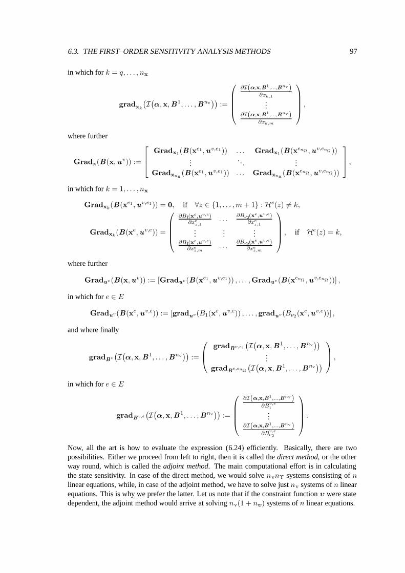
6.3. THE FIRST–ORDER SENSITIVITY ANALYSIS METHODS 97
in which for k = q, . . . , nx
gradxk
(I(α,x,B1, . . . ,Bnv
)):=
∂I(α,x,B1,...,Bnv)∂xk,1
...∂I(α,x,B1,...,Bnv)
∂xk,m
,
where further
Gradx(B(x,uv)) :=
Gradx1(B(xe1 ,uv,e1)) . . . Gradx1
(B(xenΩ ,u v,enΩ ))...
. . ....
Gradxnx
(B(xe1 ,u v,e1)) . . . Gradxnx
(B(xenΩ ,uv,enΩ ))
,
in which for k = 1, . . . , nx
Gradxk(B(xe1 ,uv,e1)) = 0, if ∀z ∈ 1, . . . ,m + 1 : He(z) 6= k,
Gradxk(B(xe,u v,e)) =
∂B1(xe,uv,e)∂xe
z,1. . .
∂Bν2(xe,uv,e)∂xe
z,1
......
...∂B1(xe,uv,e)
∂xez,m
. . .∂Bν2
(xe,uv,e)∂xe
z,m
, if He(z) = k,
where further
Graduv (B(x,uv)) := [Graduv(B(xe1 ,uv,e1)) , . . . ,Graduv(B(xenΩ ,uv,enΩ ))] ,
in which for e ∈ E
Graduv(B(xe,uv,e)) := [graduv(B1(xe,uv,e)) , . . . ,graduv(Bν2
(xe,uv,e))] ,
and where finally
gradBv
(I(α,x,B1, . . . ,Bnv
)):=
gradBv,e1
(I(α,x,B1, . . . ,Bnv
))...
gradBv,enΩ
(I(α,x,B1, . . . ,Bnv
))
,
in which for e ∈ E
gradBv,e
(I(α,x,B 1, . . . ,Bnv
)):=
∂I(α,x,B1,...,Bnv)∂Bv,e
1
...∂I(α,x,B1,...,Bnv)
∂Bv,eν2
.
Now, all the art is how to evaluate the expression (6.24) efficiently. Basically, there are twopossibilities. Either we proceed from left to right, then it is called the direct method, or the otherway round, which is called the adjoint method. The main computational effort is in calculatingthe state sensitivity. In case of the direct method, we would solve nvnΥ systems consisting of nlinear equations, while, in case of the adjoint method, we have to solve just nv systems of n linearequations. This is why we prefer the latter. Let us note that if the constraint function υ were statedependent, the adjoint method would arrive at solving nv(1 + nυ) systems of n linear equations.
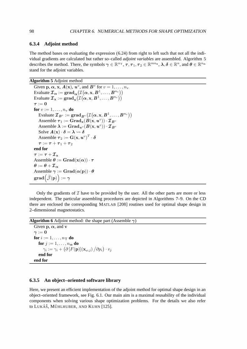
98 CHAPTER 6. NUMERICAL METHODS FOR SHAPE OPTIMIZATION
6.3.4 Adjoint method
The method bases on evaluating the expression (6.24) from right to left such that not all the indi-vidual gradients are calculated but rather so–called adjoint variables are assembled. Algorithm 5describes the method. There, the symbols γ ∈ RnΥ , τ , τ 1, τ 2 ∈ Rmnx , λ, δ ∈ Rn, and θ ∈ Rnα
stand for the adjoint variables.
Algorithm 5 Adjoint methodGiven p, α, x, A(x), u v, and Bv for v = 1, . . . , nv
Evaluate Iα := gradα
(I(α,x,B 1, . . . ,Bnv
))
Evaluate Ix := gradx
(I(α,x,B 1, . . . ,Bnv
))
τ := 0
for v := 1, . . . , nv doEvaluate IBv := gradBv
(I(α,x,B1, . . . ,Bnv
))
Assemble τ 1 := Gradx(B(x,u v)) · IBv
Assemble λ := Graduv(B(x,uv)) · IBv
Solve A(x) · δ = λ δ
Assemble τ 2 := G(x,uv)T · δτ := τ + τ 1 + τ 2
end forτ := τ + Ix
Assemble θ := Grad(x(α)) · τθ := θ + Iα
Assemble γ := Grad(α(p)) · θgrad
(J (p)
):= γ
Only the gradients of I have to be provided by the user. All the other parts are more or lessindependent. The particular assembling procedures are depicted in Algorithms 7–9. On the CDthere are enclosed the corresponding MATLAB [208] routines used for optimal shape design in2–dimensional magnetostatics.
Algorithm 6 Adjoint method: the shape part (Assemble γ)Given p, α, and v
γ := 0
for i := 1, . . . , nΥ dofor j := 1, . . . , nα do
γi := γi +(∂ [F (p)](xω,j)
/∂pi
)· vj
end forend for
6.3.5 An object–oriented software library
Here, we present an efficient implementation of the adjoint method for optimal shape design in anobject–oriented framework, see Fig. 6.1. Our main aim is a maximal reusability of the individualcomponents when solving various shape optimization problems. For the details we also referto LUKAS, MUHLHUBER, AND KUHN [125].
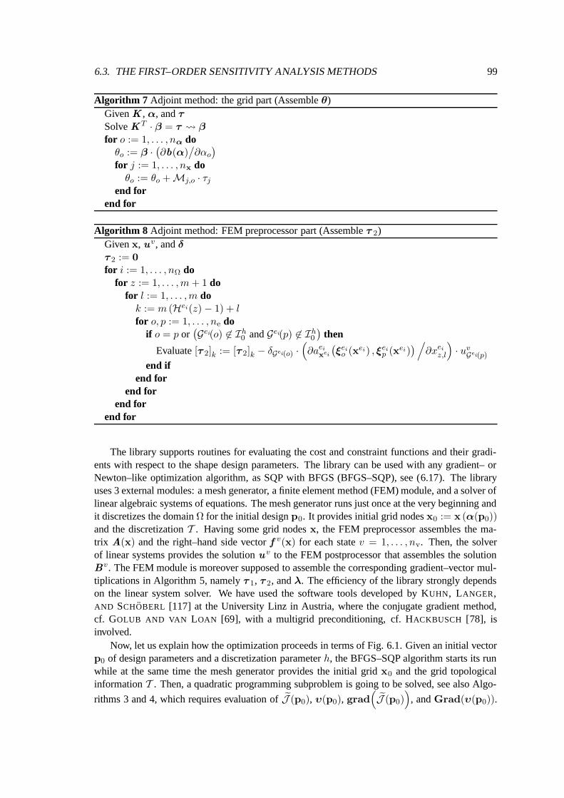
6.3. THE FIRST–ORDER SENSITIVITY ANALYSIS METHODS 99
Algorithm 7 Adjoint method: the grid part (Assemble θ)Given K , α, and τSolve K T · β = τ β
for o := 1, . . . , nα doθo := β ·
(∂b(α)
/∂αo
)
for j := 1, . . . , nx doθo := θo + Mj,o · τj
end forend for
Algorithm 8 Adjoint method: FEM preprocessor part (Assemble τ 2)Given x, uv, and δτ 2 := 0
for i := 1, . . . , nΩ dofor z := 1, . . . ,m + 1 do
for l := 1, . . . ,m dok := m (Hei(z) − 1) + lfor o, p := 1, . . . , ne do
if o = p or(Gei(o) 6∈ Ih
0 and Gei(p) 6∈ Ih0
)then
Evaluate [τ 2]k := [τ 2]k − δGei(o) ·(∂aei
xei
(ξei
o (xei) , ξeip (xei)
)/∂xei
z,l
)· uv
Gei(p)
end ifend for
end forend for
end for
The library supports routines for evaluating the cost and constraint functions and their gradi-ents with respect to the shape design parameters. The library can be used with any gradient– orNewton–like optimization algorithm, as SQP with BFGS (BFGS–SQP), see (6.17). The libraryuses 3 external modules: a mesh generator, a finite element method (FEM) module, and a solver oflinear algebraic systems of equations. The mesh generator runs just once at the very beginning andit discretizes the domain Ω for the initial design p0. It provides initial grid nodes x0 := x (α(p0))and the discretization T . Having some grid nodes x, the FEM preprocessor assembles the ma-trix A(x) and the right–hand side vector f v(x) for each state v = 1, . . . , nv. Then, the solverof linear systems provides the solution u v to the FEM postprocessor that assembles the solutionBv . The FEM module is moreover supposed to assemble the corresponding gradient–vector mul-tiplications in Algorithm 5, namely τ 1, τ 2, and λ. The efficiency of the library strongly dependson the linear system solver. We have used the software tools developed by KUHN, LANGER,AND SCHOBERL [117] at the University Linz in Austria, where the conjugate gradient method,cf. GOLUB AND VAN LOAN [69], with a multigrid preconditioning, cf. HACKBUSCH [78], isinvolved.
Now, let us explain how the optimization proceeds in terms of Fig. 6.1. Given an initial vectorp0 of design parameters and a discretization parameter h, the BFGS–SQP algorithm starts its runwhile at the same time the mesh generator provides the initial grid x0 and the grid topologicalinformation T . Then, a quadratic programming subproblem is going to be solved, see also Algo-
rithms 3 and 4, which requires evaluation of J (p0), υ(p0), grad(J (p0)
), and Grad(υ(p0)).

100 CHAPTER 6. NUMERICAL METHODS FOR SHAPE OPTIMIZATION
Algorithm 9 Adjoint method: FEM postprocessor part (Assemble τ 1, Assemble λ)Given x, uv , and IBv
τ 1 := 0
λ := 0
for i := 1, . . . , nΩ dofor z := 1, . . . ,m + 1 do
for l := 1, . . . ,m dok := m (Hei(z)) + lfor p := 1, . . . , ne do
Evaluate c := uvGei(p) ·
(∂S
ei
B(xei)/∂xei
z,l
)·Bbx
(ξr
p(x))
Evaluate d := Sei
B(xei) · Bbx
(ξr
p(x))
for j := 1, . . . , ν2 dot := ν2(i − 1) + j[τ 1]k := [τ 1]k + cj [IBv ]tλGei(p) := λGei(p) + dj [IBv ]t
end forend for
end forend for
end for
The evaluation of υ(p0) is straightforward. The evaluation of J (p0) proceeds as depicted in (6.9),where the design–to–shape mapping, shape–to–mesh mapping, FEM preprocessor, solver of lin-ear systems, FEM postprocessor, and computation of J modules take control of the run consecu-tively. Computing Grad(υ(p0)) is again quite straightforward, since it is basically an analyticalformula, which is evaluated in the module “Computation of Grad(υ(p0))”, see Fig. 6.1. Themost computationally expensive part is (together with the evaluation of the cost functional) the
evaluation of grad(J (p0)
). This evaluation follows Algorithms 5–9, where the input data flows
as depicted in Fig. 6.1. Finally, the next iteration of the BFGS–SQP algorithm is performed and theprocedure repeats for a new vector p of design parameters until a terminate criterion is fulfilled.
From the programming point of view, the only part which has always to be coded by the useris the module that computes the cost functional I
(α,x,B1, . . . ,Bnv
)and the constraint function
υ(p). Thus, we have minimized the programming effort that is necessary for solving a new shapeoptimization problem just to the specification of the problem itself.
6.3.6 A note on using the automatic differentiation
The semianalytical methods turned out to be most effective for the shape optimization, since theymake much use of the problem structure. Nevertheless, some parts of the algorithm still remainto be automatized using, e.g., the automatic differentiation (AD) method. We have in mind themodule that calculates the gradients of I and υ with respect to the input variables α, x, B v , andp, respectively. In fact, the routine calculating these gradients is just an analytical differentiationof the routine that calculates the functions I and υ. In this case, we avoid the main obstacle ofusing AD, namely, differentiation of the linear system solver. Another possible use of AD mightbe an automatic generation of routines that calculate sensitivities of the local contributions (6.22)to the system matrix A.
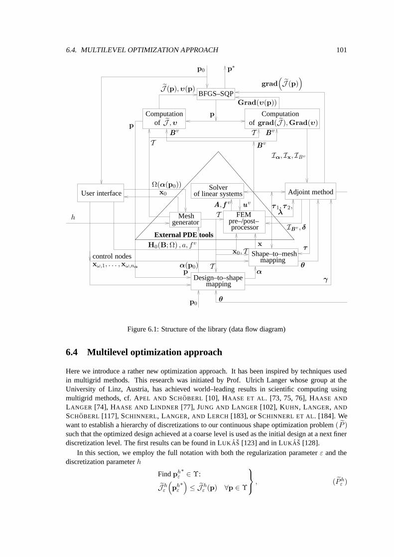
6.4. MULTILEVEL OPTIMIZATION APPROACH 101
PSfrag replacements
h
p0
p0
α(p0)
x0
x0, T
Ω(α(p0))
p∗
p
p
p
α
x
T
TT
T
J ,υ
J (p),υ(p)grad
(J (p)
)
Grad(υ(p))
grad(J ),Grad(υ)
Iα, Ix, IBv
IBv , δ
H0(B; Ω) , a, f v
A, f v uv
BvBv
Bv
τ 1, τ 2,λ
θ
θ
τ
γ
BFGS–SQP
ComputationComputationofof
User interface
External PDE tools
control nodesxω,1, . . . ,xω,nα
Design–to–shape
Shape–to–meshmapping
mapping
Adjoint methodSolver
of linear systems
Meshgenerator
FEMpre–/post–processor
Figure 6.1: Structure of the library (data flow diagram)
6.4 Multilevel optimization approach
Here we introduce a rather new optimization approach. It has been inspired by techniques usedin multigrid methods. This research was initiated by Prof. Ulrich Langer whose group at theUniversity of Linz, Austria, has achieved world–leading results in scientific computing usingmultigrid methods, cf. APEL AND SCHOBERL [10], HAASE ET AL. [73, 75, 76], HAASE AND
LANGER [74], HAASE AND LINDNER [77], JUNG AND LANGER [102], KUHN, LANGER, AND
SCHOBERL [117], SCHINNERL, LANGER, AND LERCH [183], or SCHINNERL ET AL. [184]. Wewant to establish a hierarchy of discretizations to our continuous shape optimization problem (P )such that the optimized design achieved at a coarse level is used as the initial design at a next finerdiscretization level. The first results can be found in LUKAS [123] and in LUKAS [128].
In this section, we employ the full notation with both the regularization parameter ε and thediscretization parameter h
Find phε∗ ∈ Υ:
J hε
(ph
ε∗)≤ J h
ε (p) ∀p ∈ Υ
, (P h
ε )
102 CHAPTER 6. NUMERICAL METHODS FOR SHAPE OPTIMIZATION
where J hε : Υ 7→ R denotes the discretized and regularized cost functional and
Υ := p ∈ RnΥ | υ(p) ≤ 0
is the set of admissible design parameters, where υ : RnΥ 7→ Rnυ , nυ ∈ N.By the classical optimization approach we mean the standard technique when, given a fixed
regularization parameter ε, a fixed discretization parameter h, both of which are small enough,given an initial vector p0 of design parameters, the optimization algorithm proceeds just onceending up with the optimized design ph
ε∗, see Algorithm 10.
Algorithm 10 Classical optimization approachGiven ε, h and p0
Discretize (P ) (P hε )
Solve (P hε ) with the initial design p0 ph
ε∗
phε∗
is the optimized design
By the multilevel or hierarchical optimization approach we mean that, given an initial designp1,0, we first regularize and discretize the problem (P ) at the first level with a rather large values ofε1 and h1, and the optimization algorithm proceeds ending up with a coarse optimized design ph1
ε1
∗.
Then, we refine both the regularization and the discretization parameters and run the optimizationalgorithm with smaller values of ε2 and h2 while using the design ph1
ε1
∗as the initial one at this
second level. We end up with a finer optimized design ph2
ε2
∗, and so further. The approach is
described in Algorithm 11.
Algorithm 11 Hierarchical optimization approachGiven ε1, h1, and p1,0
l := 1while l > 1 and a terminate criterion is not satisfied do
Discretize (P ) at the level l (P hlεl
)
Solve (P hlεl
) with the initial design pl,0 phlεl
∗
Refine εl, hl εl+1, hl+1
pl+1,0 := phlεl
∗
l := l + 1end whilep
hl−1
εl−1
∗is the optimized design
The hierarchical approach in shape optimization has turned out to be much more effective thanthe classical one whenever the coarse optimized design ph0
ε0
∗approximates the true one rather well.
The crucial part of the algorithm is the refinement step. The updated values of εl+1 and hl+1 mustnot be too smaller than those of εl and hl, since SQP would take many iterations. On the otherhand, if the refinement is rather coarse, i.e., the values of εl+1 and hl+1 are comparable to εl andhl, there is hardly any progress in the SQP algorithm and the hierarchical approach takes manyiterations. In Section 7.4 we provide some numerical experiments without any use of multigridyet. The idea, which we want to investigate in the future, is that the refinement strategy shouldbenefit from the aposteriori finite element error analysis and from multigrid techniques. The firstpapers in this context have appeared just recently, see RAMM, MAUTE, AND SCHWARZ [164],and SCHLEUPEN, MAUTE, AND RAMM [185]. In the paper by SCHERZER [182] a multilevelapproach is used for solving nonlinear ill–posed problems.

6.4. MULTILEVEL OPTIMIZATION APPROACH 103
Another improvement can be done, when applying the multilevel approach on the level ofmathematical modelling. It means that in those application where we can reduce the problem com-plexity by neglecting a dimension or some physical phenomena we can first solve the discretizedreduced problem and then use the result as the initial design for the more complex problem. Atypical example might be solving a shape optimization problem governed first by 2d linear mag-netostatic state problem, then, prolong the optimized design dimensionally and use it as the initialdesign for shape optimization governed by 3d linear magnetostatics, and finally use the resultingshape as the initial design for shape optimization governed by 3d nonlinear magnetostatic stateproblem. In Section 7.4, we will give a numerical test of the 2d/3d dimensional step.

104 CHAPTER 6. NUMERICAL METHODS FOR SHAPE OPTIMIZATION
Chapter 7
An application and numericalexperiments
At the beginning of this chapter, we will introduce a physical application, being of a practical use,which will lead to a problem of optimal shape design of electromagnets. Then, we will intro-duce mathematical settings of the shape optimization problems governed by linear magnetostaticmultistate problems in both two– and three–dimensional cases. We will utilize the abstract theoryintroduced in Chapters 3–5 such that we will specify all the symbols introduced in Chapter 5, val-idate the corresponding assumptions, and the related existence as well as convergence theoremswill then follow. We will also easily check Assumptions 6.1 and 6.2, both introduced in Chapter 6,which will justify us to use the SQP algorithm. Then, we will present shapes resulting from nu-merical calculations. We will also present numerical experiments with the multilevel optimizationapproach and with the adjoint method, which were both introduced in Chapter 6. We will com-pare them to the classical optimization approach and to the numerical differentiation, respectively.Some of the optimized shapes were manufactured and we are provided with physical measure-ments of the magnetic field. At the end, we will discuss magnetic field improvements in terms ofthe cost functional with respect to the original design.
The results of this chapter can be also found in PI STORA, POSTAVA, AND SEBESTA [160],KOPRIVA ET AL. [111], LUKAS [119, 120, 121, 122, 123, 128], LUKAS ET AL. [124], andin LUKAS, MUHLHUBER, AND KUHN [125].
7.1 A physical problem
Let us consider two geometries of electromagnets: the Maltese Cross (MC) geometry and the O–Ring geometry that are both depicted in Fig. 7.1. Each consists of a ferromagnetic yoke and poles.There are 4 poles in case of the Maltese Cross and 8 ones in case of the O–Ring electromagnet. Thepoles are completed with coils which are pumped with direct electric currents. The electromagnetsare used for measurements of Kerr magnetooptic effects, cf. ZVEDIN [223, p. 40]. They requirethe magnetic field as homogeneous, i.e., as constant as possible in a given normal direction. Let usnote that the magnetooptic effects are investigated for applications in high capacity data storagemedia, like a development of new media materials for magnetic or compact discs recording. Let usalso note that the electromagnets have been developed at the Institute of Physics, VSB–TechnicalUniversity of Ostrava, Czech Republic in the research group of Prof. Jaromır Pistora. Someinstances have been already delivered to the following laboratories:
105

106 CHAPTER 7. AN APPLICATION AND NUMERICAL EXPERIMENTS
Figure 7.1: The Maltese Cross and O–Ring electromagnets
• Institute of Physics, Charles University Prague, Czech Republic,
• National Institute of Applied Sciences INSA in Toulouse, France,
• Department of Physics, Simon Fraser University in Vancouver, Canada,
• Department of Chemistry, Simon Fraser University in Vancouver, Canada,
• and University Paris VI., France.
First, we describe how the Kerr magnetooptic effect is measured. Let us consider, for instance,the Maltese Cross electromagnet, as in Fig. 7.1, and its cross–section, see Fig. 7.2. A sample of
+
−
+ −
+
−
+ −
PSfrag replacements
0.2
0.2
0.15
0.1
0.1
0.05
0
0
−0.05
−0.1
−0.1
−0.15
−0.2−0.2x1 [m]
x2
[m]
magnetization magnetizationarea Ωmplanes
coil
ferromagneticyoke
pole
pole head
Figure 7.2: Cross–section of the Maltese Cross electromagnet
a magnetic material is placed into the magnetization area which is located in the middle among

7.1. A PHYSICAL PROBLEM 107
the pole heads. In this area the magnetic field is homogeneous enough with respect to the normalvector of some polarization plane, see Fig. 7.2. We pass an optical (light) beam of a given polar-ization vector to the sample. There it reflects and components of the reflected polarization vectorare measured in terms of the Kerr rotation and ellipticity, respectively. Briefly saying, we measurethe polarization state of the reflected beam. The Kerr rotation means the difference between theangle of the main ellipticity axis of the reflected beam from that one before the reflection. Typicalmeasured data is depicted in Fig. 7.3, which was measured by Ing. Igor Kopriva at the Institute ofPhysics, VSB–Technical University of Ostrava, see also KOPRIVA ET AL. [111].
*
+
PSfrag replacements
−0.2
−0.15
−0.1
−0.05
0.05
0.1
0.15
Ker
rro
tatio
n[m
rad]
0
0 20 40 60 80 100 120 140sample orientation in magnetic field [degree]
linear Kerr effectquadratic Kerr effectquadratic Kerr effect
Figure 7.3: Dependence of magnetooptic effects on a sample rotation
From Fig. 7.3 we can see that the Kerr rotation depends on the orientation of the sample inthe magnetic field, which is significant especially for the quadratic Kerr effect. This indicatesanisotropic behaviour of the sample. Therefore, we should measure it in as many directions aspossible. One has either to rotate the sample in the magnetic field, rotate the electromagnet whilethe sample is fixed, or rotate the magnetic field itself while both the sample and electromagnet arefixed. Certainly, the last variant is most preferred. The electromagnets have been developed suchthat they are capable to generate magnetic fields homogeneous in step–by–step different directionsjust by switching some currents in coils on or off, or by switching their senses. The more coils wehave, the more directions the magnetic field can be oriented in. In case of the Maltese Cross orthe O–Ring electromagnet, one can sequentially generate magnetic fields homogeneous in up to8 or 16 directions, respectively. This will lead us to a multistate problem where only the currentexcitations, i.e., the right–hand sides differ.
Our aim is to improve the current geometries of electromagnets, see Fig. 7.1, in order tobe better suited for measurements of the Kerr effect. The generated magnetic field should bestrong and homogeneous enough in order to admit a magnetooptic effect. Unfortunately, theseassumptions are contradictory and we have to balance them. From physical experience we knowthat the homogeneity of the magnetic field depends significantly on the shape of the pole heads.Hence, we aim at designing shapes of the pole heads in such a way that inhomogeneities of the

108 CHAPTER 7. AN APPLICATION AND NUMERICAL EXPERIMENTS
magnetic field are minimized, but the field itself is still strong enough.
7.2 Three–dimensional mathematical setting
Now, we introduce a complete 3d mathematical setting of the shape optimization problem. Wewill specify the abstract symbols and assumptions that were introduced in the previous text andthat are also summarized in Section 6.1. As there are no principal differences between the MalteseCross and the O–Ring electromagnet, we will describe both at once.
Convention 7.1. In all what follows the dimensions will be given in meters except for Figs. 7.5–7.7and 7.19, where they are in milimeters.
7.2.1 Geometries of the electromagnets
The computational domain is fixed and in case of the Maltese Cross and the O–Ring it is, respec-tively, as follows:
Ω :=
(−d1
2,d1
2
)×(−d2
2,d2
2
)×(−d3
2,d3
2
)
and
Ω :=
x := (x1, x2, x3) ∈ R3
∣∣∣∣ (x1)2 + (x2)
2 < (r)2 and |x3| <d3
2
,
whered1 := d2 := 0.4 [m], d3 := 0.02 [m], r := 0.2 [m].
The computational domain obviously fulfills Assumption 3.1 and Ω ∈ L.We describe the geometrical models of the electromagnets. Referring to Fig. 7.4, the green
Figure 7.4: Geometrical models of the Maltese Cross and O–Ring electromagnets
parts are the ferromagnetic yoke and the poles. The blue parts are the coils. In Fig. 7.5 and inFig. 7.6 we can see dimensions in milimeters for geometrical models of the Maltese Cross andof the O–Ring electromagnet, respectively. The symbol Ωyoke stands for the domain occupied bythe ferromagnetic yoke, the symbols Ωwestp, Ωnorthwestp, Ωnorthp, Ωnortheastp, Ωeastp, Ωsoutheastp,Ωsouthp, and Ωsouthwestp denote the domains occupied by the particular poles, and the symbolsΩwestc, Ωnorthwestc, Ωnorthc, Ωnortheastc, Ωeastc, Ωsoutheastc, Ωsouthc, and Ωsouthwestc denote thedomains that are occupied by the corresponding coils. In Fig. 7.7 we can see the west pole of
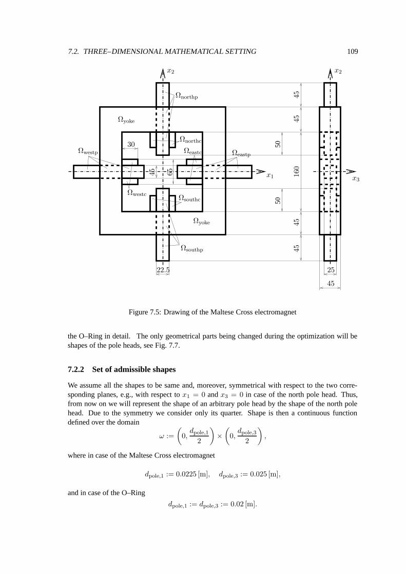
7.2. THREE–DIMENSIONAL MATHEMATICAL SETTING 109
5050
PSfrag replacements
x1
x2x2
x3
Ωyoke
Ωyoke
Ωwestp
Ωnorthp
Ωeastp
Ωsouthp
Ωwestc
Ωnorthc
Ωeastc
Ωsouthc
22.5 25
30
45
4545
45
4545
65 160
Figure 7.5: Drawing of the Maltese Cross electromagnet
the O–Ring in detail. The only geometrical parts being changed during the optimization will beshapes of the pole heads, see Fig. 7.7.
7.2.2 Set of admissible shapes
We assume all the shapes to be same and, moreover, symmetrical with respect to the two corre-sponding planes, e.g., with respect to x1 = 0 and x3 = 0 in case of the north pole head. Thus,from now on we will represent the shape of an arbitrary pole head by the shape of the north polehead. Due to the symmetry we consider only its quarter. Shape is then a continuous functiondefined over the domain
ω :=
(0,
dpole,1
2
)×(
0,dpole,3
2
),
where in case of the Maltese Cross electromagnet
dpole,1 := 0.0225 [m], dpole,3 := 0.025 [m],
and in case of the O–Ring
dpole,1 := dpole,3 := 0.02 [m].
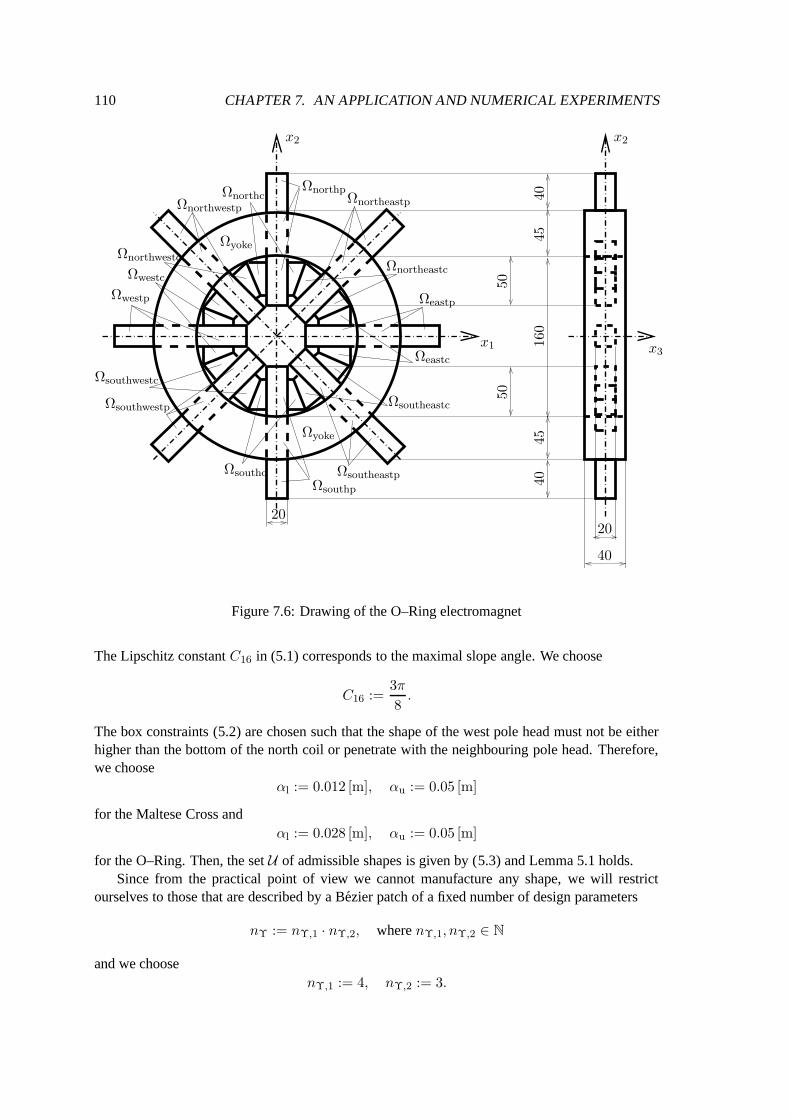
110 CHAPTER 7. AN APPLICATION AND NUMERICAL EXPERIMENTSPSfrag replacements
x1
x2x2
x3
Ωyoke
Ωyoke
Ωwestp
Ωnorthwestp
ΩnorthpΩnortheastp
Ωeastp
ΩsoutheastpΩsouthp
Ωsouthwestp
Ωwestc
Ωnorthwestc
Ωnorthc
Ωnortheastc
Ωeastc
Ωsoutheastc
Ωsouthc
Ωsouthwestc
2020
4040
4045
45
5050
160
Figure 7.6: Drawing of the O–Ring electromagnet
The Lipschitz constant C16 in (5.1) corresponds to the maximal slope angle. We choose
C16 :=3π
8.
The box constraints (5.2) are chosen such that the shape of the west pole head must not be eitherhigher than the bottom of the north coil or penetrate with the neighbouring pole head. Therefore,we choose
αl := 0.012 [m], αu := 0.05 [m]
for the Maltese Cross andαl := 0.028 [m], αu := 0.05 [m]
for the O–Ring. Then, the set U of admissible shapes is given by (5.3) and Lemma 5.1 holds.Since from the practical point of view we cannot manufacture any shape, we will restrict
ourselves to those that are described by a Bezier patch of a fixed number of design parameters
nΥ := nΥ,1 · nΥ,2, where nΥ,1, nΥ,2 ∈ N
and we choosenΥ,1 := 4, nΥ,2 := 3.
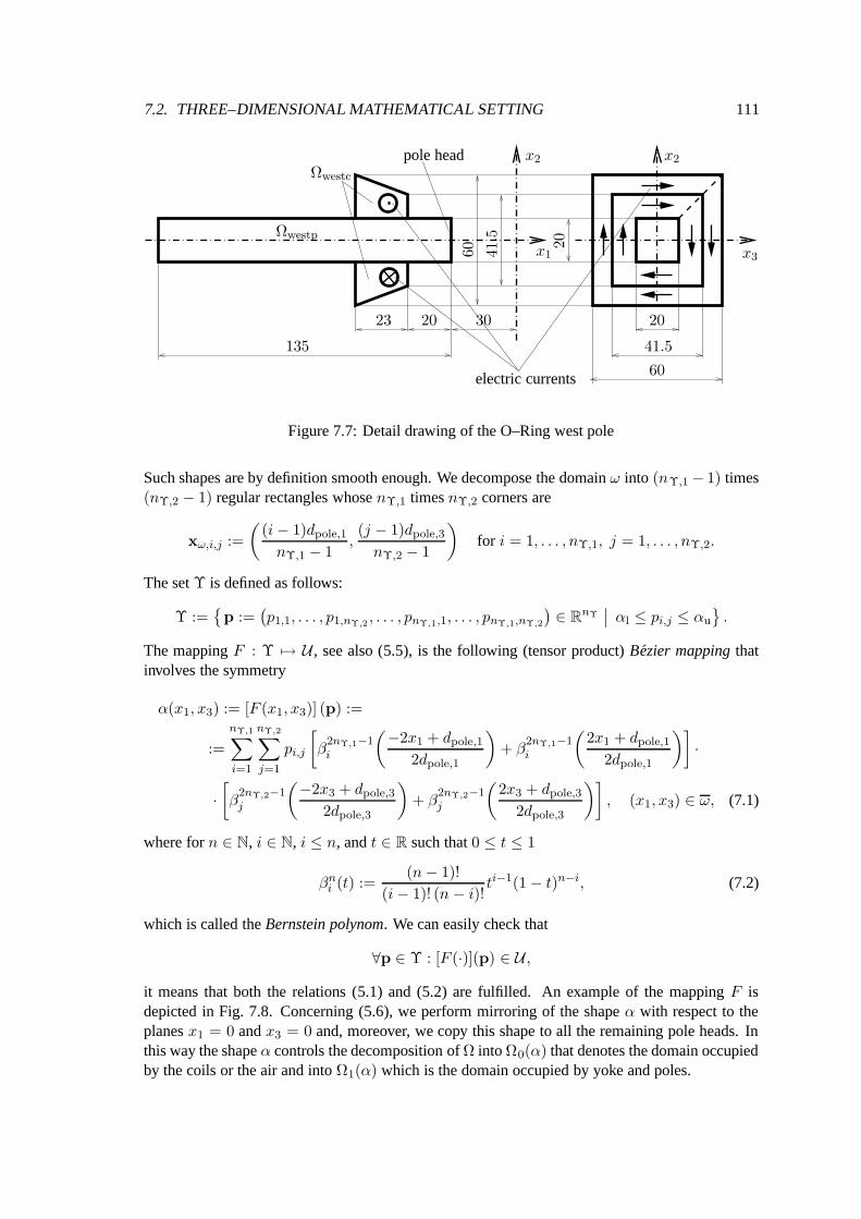
7.2. THREE–DIMENSIONAL MATHEMATICAL SETTING 111PSfrag replacements
x1
x2x2
x3
Ωwestp
Ωwestc
20
20 2023 30
41.5
41.5
60
60
135
pole head
electric currents
Figure 7.7: Detail drawing of the O–Ring west pole
Such shapes are by definition smooth enough. We decompose the domain ω into (nΥ,1 − 1) times(nΥ,2 − 1) regular rectangles whose nΥ,1 times nΥ,2 corners are
xω,i,j :=
((i − 1)dpole,1
nΥ,1 − 1,(j − 1)dpole,3
nΥ,2 − 1
)for i = 1, . . . , nΥ,1, j = 1, . . . , nΥ,2.
The set Υ is defined as follows:
Υ :=p :=
(p1,1, . . . , p1,nΥ,2
, . . . , pnΥ,1,1, . . . , pnΥ,1,nΥ,2
)∈ RnΥ
∣∣ αl ≤ pi,j ≤ αu
.
The mapping F : Υ 7→ U , see also (5.5), is the following (tensor product) Bezier mapping thatinvolves the symmetry
α(x1, x3) := [F (x1, x3)] (p) :=
:=
nΥ,1∑
i=1
nΥ,2∑
j=1
pi,j
[β
2nΥ,1−1i
(−2x1 + dpole,1
2dpole,1
)+ β
2nΥ,1−1i
(2x1 + dpole,1
2dpole,1
)]·
·[β
2nΥ,2−1j
(−2x3 + dpole,3
2dpole,3
)+ β
2nΥ,2−1j
(2x3 + dpole,3
2dpole,3
)], (x1, x3) ∈ ω, (7.1)
where for n ∈ N, i ∈ N, i ≤ n, and t ∈ R such that 0 ≤ t ≤ 1
βni (t) :=
(n − 1)!
(i − 1)! (n − i)!ti−1(1 − t)n−i, (7.2)
which is called the Bernstein polynom. We can easily check that
∀p ∈ Υ : [F (·)](p) ∈ U ,
it means that both the relations (5.1) and (5.2) are fulfilled. An example of the mapping F isdepicted in Fig. 7.8. Concerning (5.6), we perform mirroring of the shape α with respect to theplanes x1 = 0 and x3 = 0 and, moreover, we copy this shape to all the remaining pole heads. Inthis way the shape α controls the decomposition of Ω into Ω0(α) that denotes the domain occupiedby the coils or the air and into Ω1(α) which is the domain occupied by yoke and poles.
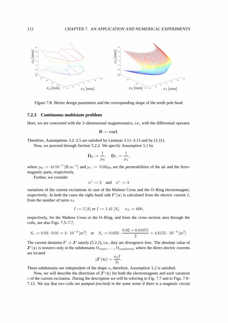
112 CHAPTER 7. AN APPLICATION AND NUMERICAL EXPERIMENTS
−15−10
−50
510
15
5
10
15
20
25
30−15
−10
−5
0
5
10
15
PSfrag replacements
x1 [mm]x2 [mm]
x3[m
m]
−15−10
−50
510
15
15
20
25
30−15
−10
−5
0
5
10
15
PSfrag replacements
x1 [mm]x2 [mm]
x3[m
m]
Figure 7.8: Bezier design parameters and the corresponding shape of the north pole head
7.2.3 Continuous multistate problem
Here, we are concerned with the 3–dimensional magnetostatics, i.e., with the differential operator
B := curl.
Therefore, Assumptions 3.2–3.5 are satisfied by Lemmas 3.11–3.13 and by (3.31).Now, we proceed through Section 5.2.2. We specify Assumption 5.1 by
D0 :=1
µ0, D1 :=
1
µ1,
where µ0 := 4π10−7 [H.m−1] and µ1 := 5100µ0 are the permeabilities of the air and the ferro-magnetic parts, respectively.
Further, we considernv := 2 and nv := 3
variations of the current excitations in case of the Maltese Cross and the O–Ring electromagnet,respectively. In both the cases the right–hand side f v(x) is calculated from the electric current I ,from the number of turns nI
I := 5 [A] or I := 1.41 [A], nI := 600,
respectively, for the Maltese Cross or the O–Ring, and from the cross–section area through thecoils, see also Figs. 7.5–7.7,
Sc := 0.03 · 0.01 = 3 · 10−4 [m2] or Sc := 0.023 · 0.02 + 0.01075
2= 4.6125 · 10−4 [m2].
The current densities f v ≡ Jv satisfy (5.2.2), i.e., they are divergence–free. The absolute value ofJv(x) is nonzero only in the subdomains Ωwestc, . . . , Ωsouthwestc where the direct electric currentsare located
|Jv(x)| =nII
Sc.
These subdomains are independent of the shape α, therefore, Assumption 5.2 is satisfied.Now, we will describe the directions of Jv(x) for both the electromagnets and each variation
v of the current excitation. During the description we will be referring to Fig. 7.7 and to Figs. 7.9–7.13. We say that two coils are pumped (excited) in the same sense if there is a magnetic circuit
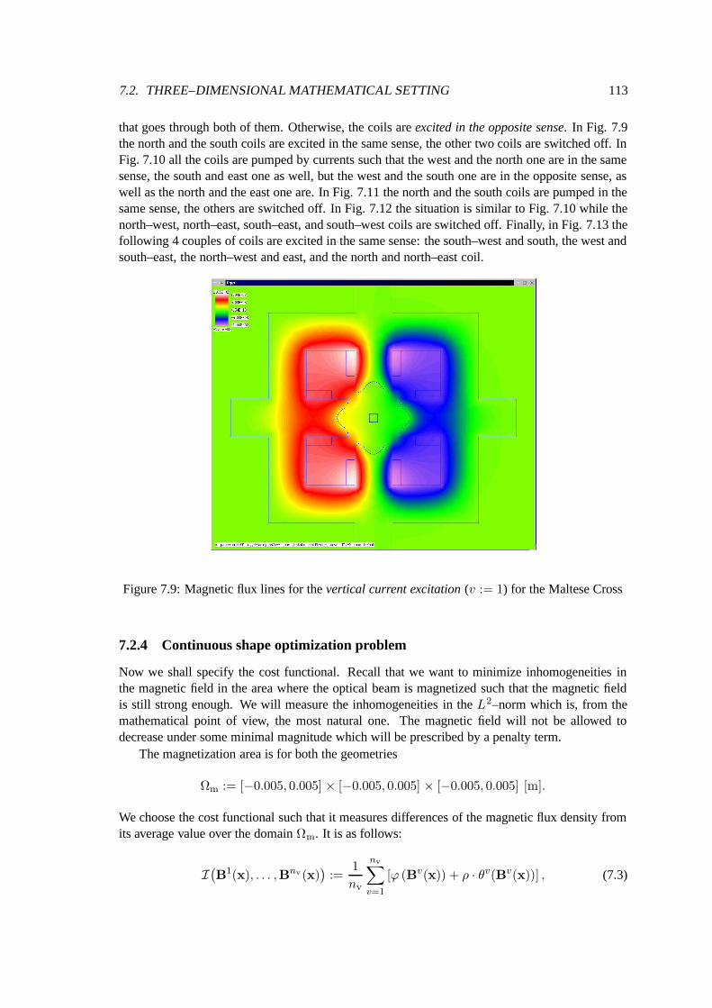
7.2. THREE–DIMENSIONAL MATHEMATICAL SETTING 113
that goes through both of them. Otherwise, the coils are excited in the opposite sense. In Fig. 7.9the north and the south coils are excited in the same sense, the other two coils are switched off. InFig. 7.10 all the coils are pumped by currents such that the west and the north one are in the samesense, the south and east one as well, but the west and the south one are in the opposite sense, aswell as the north and the east one are. In Fig. 7.11 the north and the south coils are pumped in thesame sense, the others are switched off. In Fig. 7.12 the situation is similar to Fig. 7.10 while thenorth–west, north–east, south–east, and south–west coils are switched off. Finally, in Fig. 7.13 thefollowing 4 couples of coils are excited in the same sense: the south–west and south, the west andsouth–east, the north–west and east, and the north and north–east coil.
Figure 7.9: Magnetic flux lines for the vertical current excitation (v := 1) for the Maltese Cross
7.2.4 Continuous shape optimization problem
Now we shall specify the cost functional. Recall that we want to minimize inhomogeneities inthe magnetic field in the area where the optical beam is magnetized such that the magnetic fieldis still strong enough. We will measure the inhomogeneities in the L2–norm which is, from themathematical point of view, the most natural one. The magnetic field will not be allowed todecrease under some minimal magnitude which will be prescribed by a penalty term.
The magnetization area is for both the geometries
Ωm := [−0.005, 0.005] × [−0.005, 0.005] × [−0.005, 0.005] [m].
We choose the cost functional such that it measures differences of the magnetic flux density fromits average value over the domain Ωm. It is as follows:
I(B1(x), . . . ,Bnv(x)
):=
1
nv
nv∑
v=1
[ϕ (Bv(x)) + ρ · θv(Bv(x))] , (7.3)
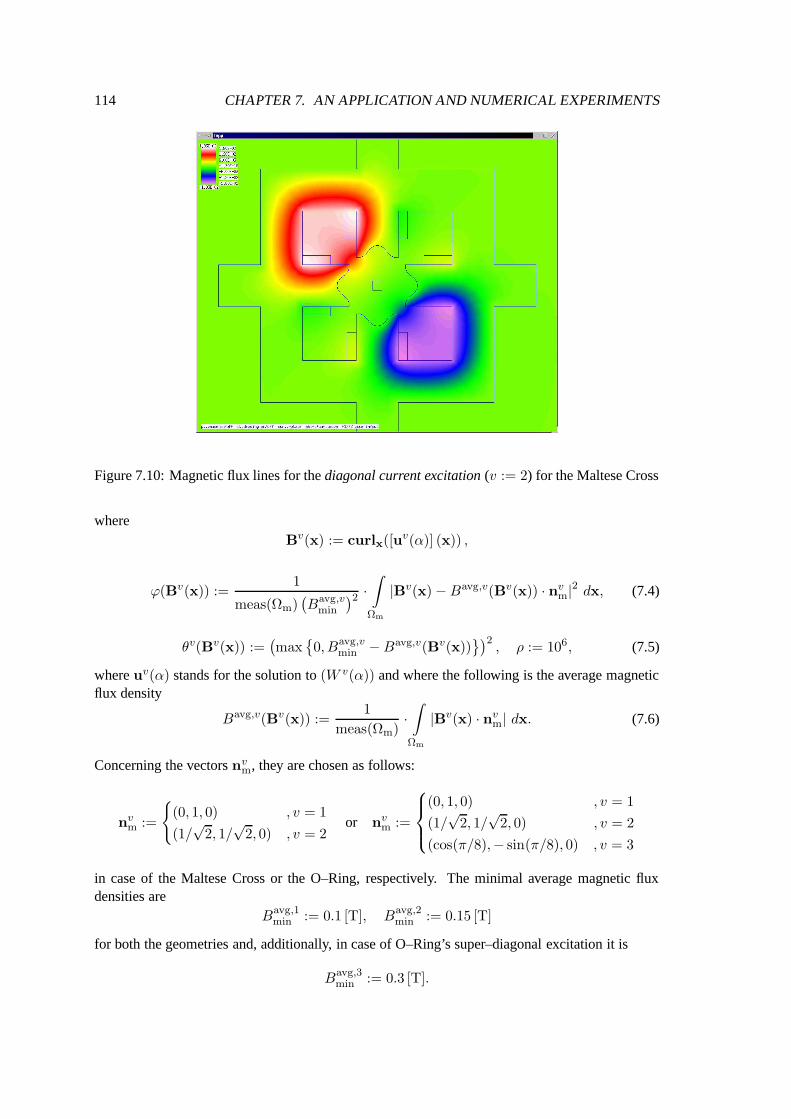
114 CHAPTER 7. AN APPLICATION AND NUMERICAL EXPERIMENTS
Figure 7.10: Magnetic flux lines for the diagonal current excitation (v := 2) for the Maltese Cross
whereBv(x) := curlx([uv(α)] (x)) ,
ϕ(Bv(x)) :=1
meas(Ωm)(Bavg,v
min
)2 ·∫
Ωm
|Bv(x) − Bavg,v(Bv(x)) · nvm|2 dx, (7.4)
θv(Bv(x)) :=(max
0, Bavg,v
min − Bavg,v(Bv(x)))2
, ρ := 106, (7.5)
where uv(α) stands for the solution to (W v(α)) and where the following is the average magneticflux density
Bavg,v(Bv(x)) :=1
meas(Ωm)·∫
Ωm
|Bv(x) · nvm| dx. (7.6)
Concerning the vectors nvm, they are chosen as follows:
nvm :=
(0, 1, 0) , v = 1
(1/√
2, 1/√
2, 0) , v = 2or nv
m :=
(0, 1, 0) , v = 1
(1/√
2, 1/√
2, 0) , v = 2
(cos(π/8),− sin(π/8), 0) , v = 3
in case of the Maltese Cross or the O–Ring, respectively. The minimal average magnetic fluxdensities are
Bavg,1min := 0.1 [T], Bavg,2
min := 0.15 [T]
for both the geometries and, additionally, in case of O–Ring’s super–diagonal excitation it is
Bavg,3min := 0.3 [T].
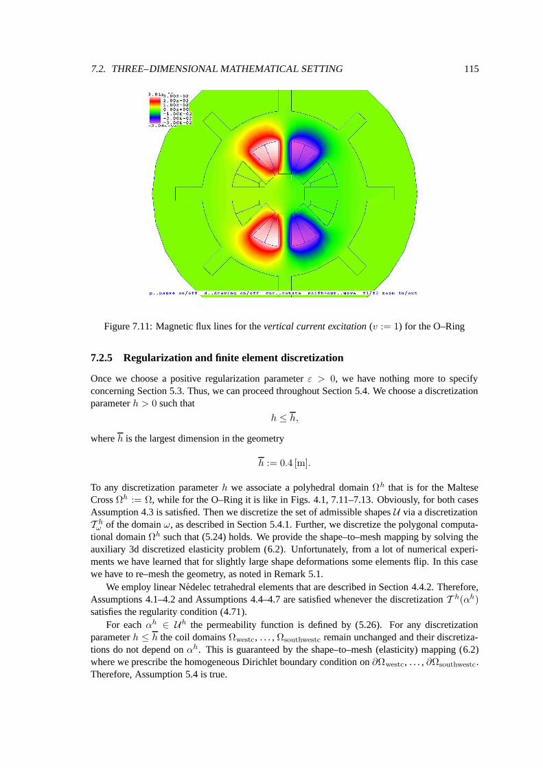
7.2. THREE–DIMENSIONAL MATHEMATICAL SETTING 115
Figure 7.11: Magnetic flux lines for the vertical current excitation (v := 1) for the O–Ring
7.2.5 Regularization and finite element discretization
Once we choose a positive regularization parameter ε > 0, we have nothing more to specifyconcerning Section 5.3. Thus, we can proceed throughout Section 5.4. We choose a discretizationparameter h > 0 such that
h ≤ h,
where h is the largest dimension in the geometry
h := 0.4 [m].
To any discretization parameter h we associate a polyhedral domain Ωh that is for the MalteseCross Ωh := Ω, while for the O–Ring it is like in Figs. 4.1, 7.11–7.13. Obviously, for both casesAssumption 4.3 is satisfied. Then we discretize the set of admissible shapes U via a discretizationT h
ω of the domain ω, as described in Section 5.4.1. Further, we discretize the polygonal computa-tional domain Ωh such that (5.24) holds. We provide the shape–to–mesh mapping by solving theauxiliary 3d discretized elasticity problem (6.2). Unfortunately, from a lot of numerical experi-ments we have learned that for slightly large shape deformations some elements flip. In this casewe have to re–mesh the geometry, as noted in Remark 5.1.
We employ linear Nedelec tetrahedral elements that are described in Section 4.4.2. Therefore,Assumptions 4.1–4.2 and Assumptions 4.4–4.7 are satisfied whenever the discretization T h(αh)satisfies the regularity condition (4.71).
For each αh ∈ Uh the permeability function is defined by (5.26). For any discretizationparameter h ≤ h the coil domains Ωwestc, . . . , Ωsouthwestc remain unchanged and their discretiza-tions do not depend on αh. This is guaranteed by the shape–to–mesh (elasticity) mapping (6.2)where we prescribe the homogeneous Dirichlet boundary condition on ∂Ωwestc, . . . , ∂Ωsouthwestc.Therefore, Assumption 5.4 is true.
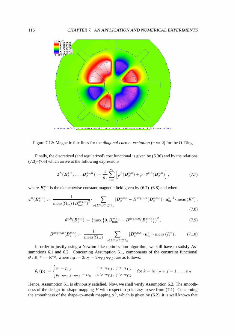
116 CHAPTER 7. AN APPLICATION AND NUMERICAL EXPERIMENTS
Figure 7.12: Magnetic flux lines for the diagonal current excitation (v := 2) for the O–Ring
Finally, the discretized (and regularized) cost functional is given by (5.36) and by the relations(7.3)–(7.6) which arrive at the following expressions
Ih(B1,n
ε , . . . ,Bnv,nε
):=
1
nv
nv∑
v=1
[ϕh(Bv,n
ε ) + ρ · θv,h(Bv,nε )], (7.7)
where B v,nε is the elementwise constant magnetic field given by (6.7)–(6.8) and where
ϕh(Bv,nε ) :=
1
meas(Ωm)(Bavg,v
min
)2 ·∑
e∈Eh:Ke⊂Ωm
|Bv,n,eε − Bavg,v,n(Bv,n,e
ε ) · nvm|2 ·meas (Ke) ,
(7.8)
θv,h(Bv,nε ) :=
(max
0, Bavg,v
min − Bavg,v,n(Bv,nε ))2
, (7.9)
Bavg,v,n(Bv,nε ) :=
1
meas(Ωm)·
∑
e∈Eh:Ke⊂Ωm
|Bv,n,eε · nv
m| · meas (Ke) . (7.10)
In order to justify using a Newton–like optimization algorithm, we still have to satisfy As-sumptions 6.1 and 6.2. Concerning Assumption 6.1, components of the constraint functionalθ : RnΥ 7→ Rnθ , where nθ := 2nΥ = 2nΥ,1nΥ,2, are as follows:
θk(p) :=
αl − pi,j , i ≤ nΥ,1, j ≤ nΥ,2
pi−nΥ,1,j−nΥ,2− αu , i > nΥ,1, j > nΥ,2
for k = inΥ,2 + j = 1, . . . , nθ
Hence, Assumption 6.1 is obviously satisfied. Now, we shall verify Assumption 6.2. The smooth-ness of the design–to–shape mapping F with respect to p is easy to see from (7.1). Concerningthe smoothness of the shape–to–mesh mapping xh, which is given by (6.2), it is well known that

7.3. TWO–DIMENSIONAL MATHEMATICAL SETTING 117
Figure 7.13: Magnetic flux lines for the super–diagonal current excitation (v := 3) for the O–Ring
the stiffness matrix K h(x0) is nonsingular as far as we consider a Dirichlet boundary conditionat a certain part of either the boundary ∂Ωh or an interface ∂Ωh
0(αh) ∩ ∂Ωh1(αh). Since bh
(αh)
involves the following nonhomogeneous Dirichlet design interface boundary condition
4xh = Mh ·αh on Γαh ,
where Γαh denotes the design interface, then, xh, see (6.2), is smooth with respect to αh. Fur-ther, due to (4.66), (4.68), and (4.69) we can see that each of Re(xe), Se(xe), and Se
curl(xe),
respectively, is smooth as far as Ke does not flip. The last item of Assumption 6.2 easily followsfrom (7.7)–(7.10).
7.3 Two–dimensional mathematical setting
Here, we reduce our mathematical model by neglecting the third dimension of the geometry,as described in Section 2.3. Thus, each 2–dimensional domain, denoted formally by Ω2d, iscreated as the intersection of the related 3–dimensional domain Ω with the zero plane Z :=x ∈ R3 | x3 = 0
and by skipping the third component, i.e.,
Ω2d :=x := (x1, x2) ∈ R2 | (x1, x2, 0) ∈ Ω
.
We consider
ω :=
(0,
dpole,1
2
).
The Lipschitz constant as well as the box constraints remain. The set of admissible shapes is givenby (5.3).
Concerning Υ, we choose the following number of design parameters
nΥ := nΥ,1 := 4,
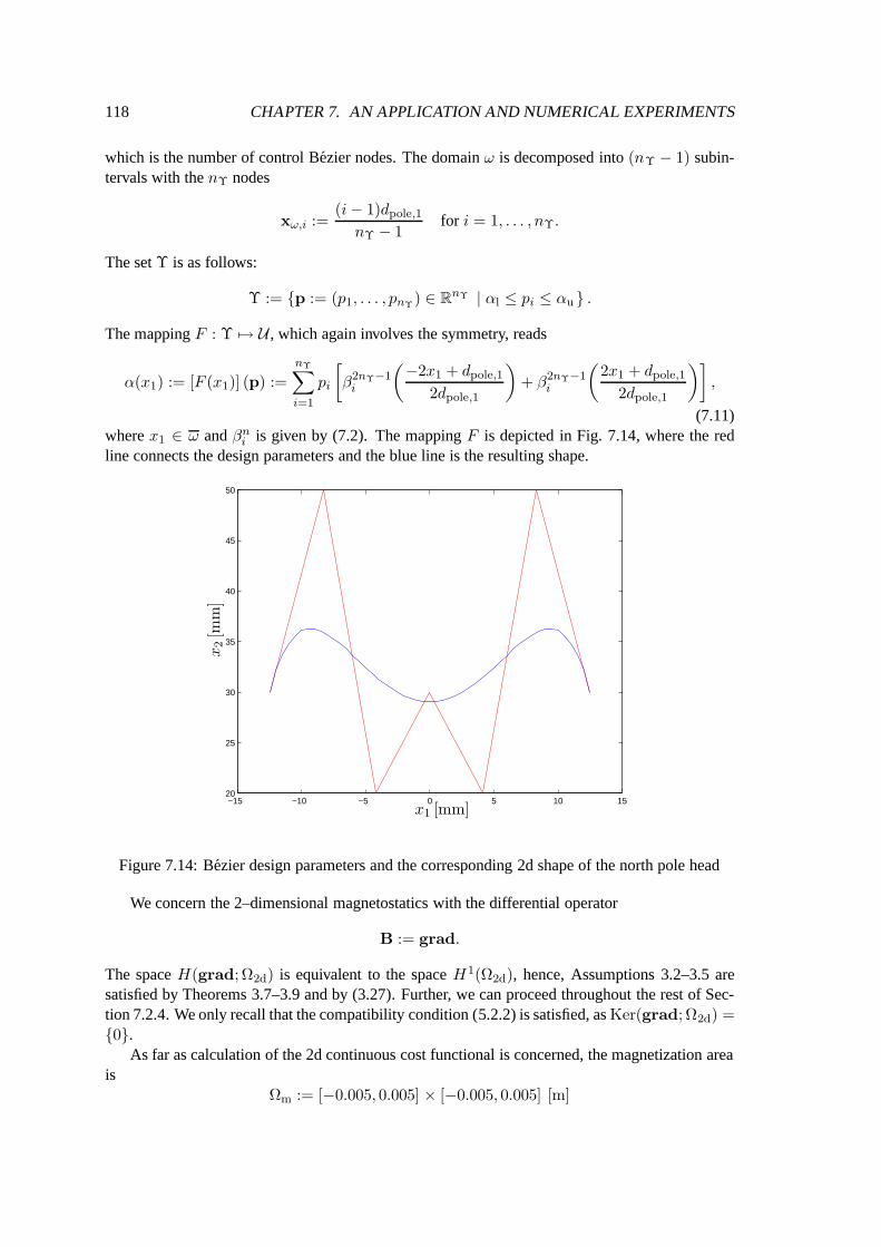
118 CHAPTER 7. AN APPLICATION AND NUMERICAL EXPERIMENTS
which is the number of control Bezier nodes. The domain ω is decomposed into (nΥ − 1) subin-tervals with the nΥ nodes
xω,i :=(i − 1)dpole,1
nΥ − 1for i = 1, . . . , nΥ.
The set Υ is as follows:
Υ := p := (p1, . . . , pnΥ) ∈ RnΥ | αl ≤ pi ≤ αu .
The mapping F : Υ 7→ U , which again involves the symmetry, reads
α(x1) := [F (x1)] (p) :=
nΥ∑
i=1
pi
[β2nΥ−1
i
(−2x1 + dpole,1
2dpole,1
)+ β2nΥ−1
i
(2x1 + dpole,1
2dpole,1
)],
(7.11)where x1 ∈ ω and βn
i is given by (7.2). The mapping F is depicted in Fig. 7.14, where the redline connects the design parameters and the blue line is the resulting shape.
−15 −10 −5 0 5 10 1520
25
30
35
40
45
50
PSfrag replacements
x1 [mm]
x2[m
m]
Figure 7.14: Bezier design parameters and the corresponding 2d shape of the north pole head
We concern the 2–dimensional magnetostatics with the differential operator
B := grad.
The space H(grad; Ω2d) is equivalent to the space H1(Ω2d), hence, Assumptions 3.2–3.5 aresatisfied by Theorems 3.7–3.9 and by (3.27). Further, we can proceed throughout the rest of Sec-tion 7.2.4. We only recall that the compatibility condition (5.2.2) is satisfied, as Ker(grad; Ω2d) =0.
As far as calculation of the 2d continuous cost functional is concerned, the magnetization areais
Ωm := [−0.005, 0.005] × [−0.005, 0.005] [m]
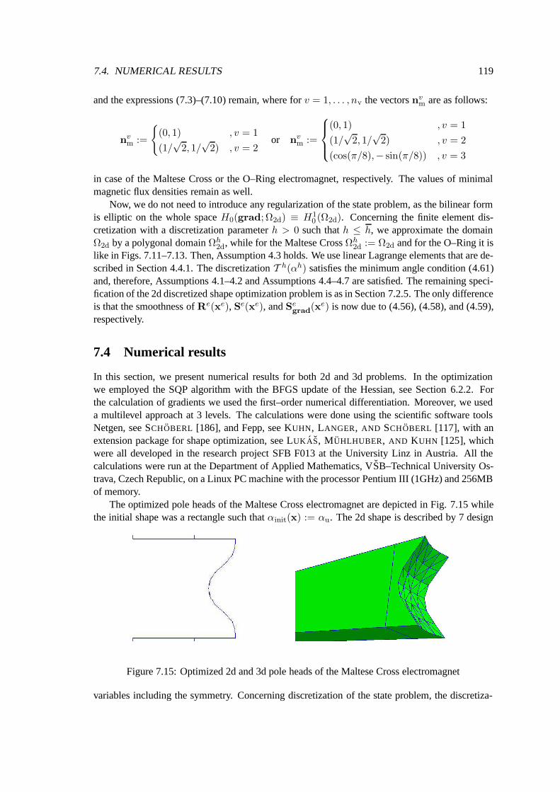
7.4. NUMERICAL RESULTS 119
and the expressions (7.3)–(7.10) remain, where for v = 1, . . . , nv the vectors nvm are as follows:
nvm :=
(0, 1) , v = 1
(1/√
2, 1/√
2) , v = 2or nv
m :=
(0, 1) , v = 1
(1/√
2, 1/√
2) , v = 2
(cos(π/8),− sin(π/8)) , v = 3
in case of the Maltese Cross or the O–Ring electromagnet, respectively. The values of minimalmagnetic flux densities remain as well.
Now, we do not need to introduce any regularization of the state problem, as the bilinear formis elliptic on the whole space H0(grad; Ω2d) ≡ H1
0 (Ω2d). Concerning the finite element dis-cretization with a discretization parameter h > 0 such that h ≤ h, we approximate the domainΩ2d by a polygonal domain Ωh
2d, while for the Maltese Cross Ωh2d := Ω2d and for the O–Ring it is
like in Figs. 7.11–7.13. Then, Assumption 4.3 holds. We use linear Lagrange elements that are de-scribed in Section 4.4.1. The discretization T h(αh) satisfies the minimum angle condition (4.61)and, therefore, Assumptions 4.1–4.2 and Assumptions 4.4–4.7 are satisfied. The remaining speci-fication of the 2d discretized shape optimization problem is as in Section 7.2.5. The only differenceis that the smoothness of Re(xe), Se(xe), and Se
grad(xe) is now due to (4.56), (4.58), and (4.59),respectively.
7.4 Numerical results
In this section, we present numerical results for both 2d and 3d problems. In the optimizationwe employed the SQP algorithm with the BFGS update of the Hessian, see Section 6.2.2. Forthe calculation of gradients we used the first–order numerical differentiation. Moreover, we useda multilevel approach at 3 levels. The calculations were done using the scientific software toolsNetgen, see SCHOBERL [186], and Fepp, see KUHN, LANGER, AND SCHOBERL [117], with anextension package for shape optimization, see LUKAS, MUHLHUBER, AND KUHN [125], whichwere all developed in the research project SFB F013 at the University Linz in Austria. All thecalculations were run at the Department of Applied Mathematics, VSB–Technical University Os-trava, Czech Republic, on a Linux PC machine with the processor Pentium III (1GHz) and 256MBof memory.
The optimized pole heads of the Maltese Cross electromagnet are depicted in Fig. 7.15 whilethe initial shape was a rectangle such that αinit(x) := αu. The 2d shape is described by 7 design
Figure 7.15: Optimized 2d and 3d pole heads of the Maltese Cross electromagnet
variables including the symmetry. Concerning discretization of the state problem, the discretiza-

120 CHAPTER 7. AN APPLICATION AND NUMERICAL EXPERIMENTS
tion parameters are
h := 0.05 [m], h := 0.025 [m], and h := 0.0125 [m]
at the first (coarsest), second, and third (finest) level, respectively. There are 12272 degrees offreedom at the last (3rd, finest) level. The optimization took 8 SQP iterations at the first (coarsest)level, 35 ones at the second level, and 25 ones at the third (finest) level, which was all done in 1hour and 59 minutes, see also Fig. 7.17. The cost functional decreased from 1.97 · 10−6 (1st level)to 1.49 · 10−6 (3rd level). The 3d shape is determined by 12 design variables with the symmetryinvolved. The state problem at the finest level is discretized by 29541 degrees of freedom. Withinthe multilevel approach we made a step between the 2d and 3d model such that at the first level wehad a coarse discretization of the 2d problem, at the second level we had a coarse discretizationof the 3d problem, and at the last third level we had a fine discretization of the 3d problem. Thecalculation proceeded in 6, 50, and 37 SQP iterations at the respective levels, i.e., 93 SQP iterationsin total, which took 29 hours and 46 minutes, see also Fig. 7.18. The cost functional decreasedfrom 2.57 · 10−6 (2nd level) to 7.32 · 10−7 (3rd level).
The 2d optimized pole head of the O–Ring electromagnet is depicted in Fig. 7.16 while theinitial shape was again a rectangle. The shape is described by 7 design variables including the
Figure 7.16: Optimized 2d pole head of the O–Ring electromagnet
symmetry. The state problem has 12005 degrees of freedom at the third (finest) level. The opti-mization took 19, 8, and 37 SQP iterations at the respective levels, which means 64 iterations intotal and it was all done in 3 hours and 41 minutes. The cost functional decreased from 8.14 ·10−4
(1st, coarsest level) to 2.87 · 10−4 (3rd, finest level).
7.4.1 Testing the multilevel approach
Here, we present numerical tests of the multilevel optimization approach that was introduced inSection 6.4. We refer to Fig. 7.17, where we compare the multilevel approach with the classicalone. We apply them to the 2d Maltese Cross optimization problem. From the last column inFig. 7.17, we can see that the multilevel approach is much faster than the classical one. Using themultilevel approach, the calculation took about 2 hours while it took almost 7 hours, when usingthe classical approach.
In Fig. 7.18, a general multilevel approach is presented. It is tested on the 3d optimal shapedesign problem of the Maltese Cross electromagnet. At the first level (h := 0.05 [m]), a coarse 2doptimization proceeds from the initial rectangular shape. The 2d coarse optimized shape from thefirst level is used as the initial guess at the second level, where a coarse (h := 0.05 [m]), but now,
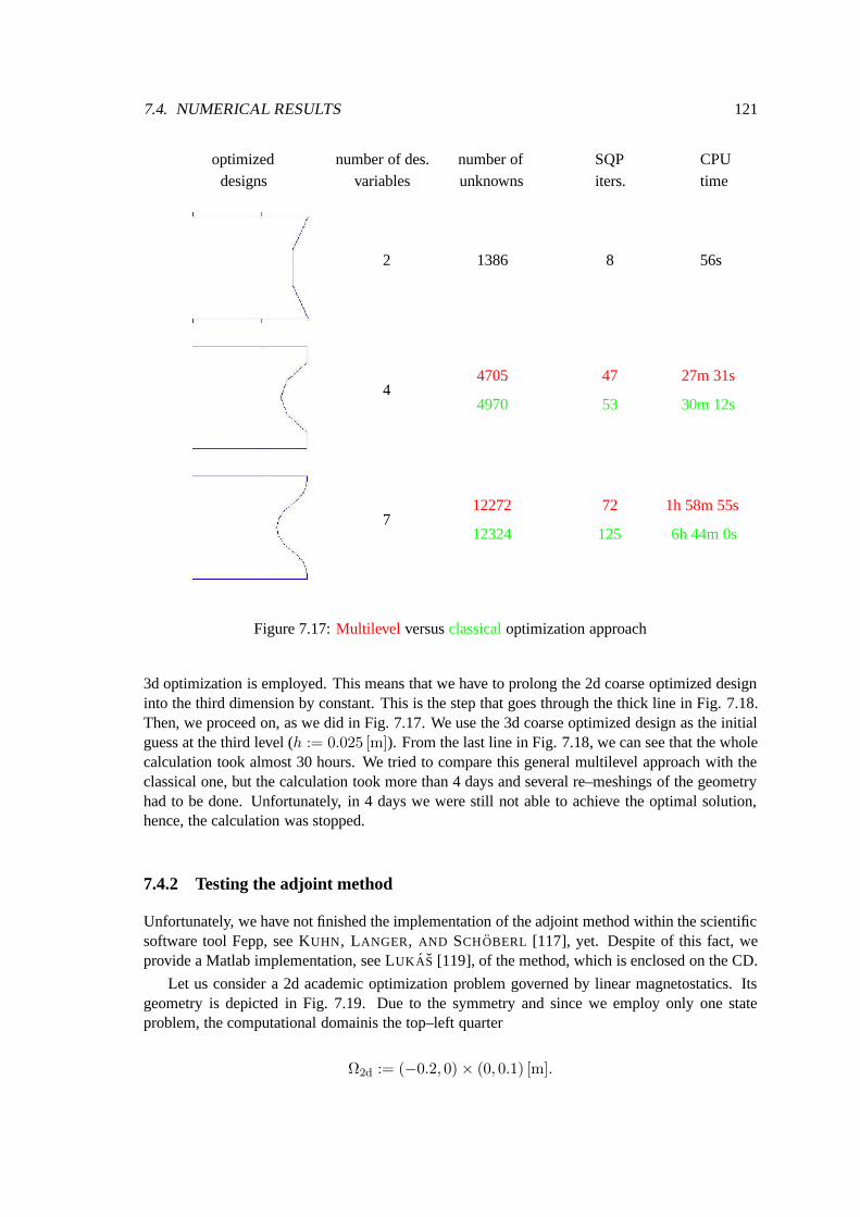
7.4. NUMERICAL RESULTS 121
optimizeddesigns
number of des.variables
number ofunknowns
SQPiters.
CPUtime
2 1386 8 56s
44705
4970
47
53
27m 31s
30m 12s
712272
12324
72
125
1h 58m 55s
6h 44m 0s
Figure 7.17: Multilevel versus classical optimization approach
3d optimization is employed. This means that we have to prolong the 2d coarse optimized designinto the third dimension by constant. This is the step that goes through the thick line in Fig. 7.18.Then, we proceed on, as we did in Fig. 7.17. We use the 3d coarse optimized design as the initialguess at the third level (h := 0.025 [m]). From the last line in Fig. 7.18, we can see that the wholecalculation took almost 30 hours. We tried to compare this general multilevel approach with theclassical one, but the calculation took more than 4 days and several re–meshings of the geometryhad to be done. Unfortunately, in 4 days we were still not able to achieve the optimal solution,hence, the calculation was stopped.
7.4.2 Testing the adjoint method
Unfortunately, we have not finished the implementation of the adjoint method within the scientificsoftware tool Fepp, see KUHN, LANGER, AND SCHOBERL [117], yet. Despite of this fact, weprovide a Matlab implementation, see LUKAS [119], of the method, which is enclosed on the CD.
Let us consider a 2d academic optimization problem governed by linear magnetostatics. Itsgeometry is depicted in Fig. 7.19. Due to the symmetry and since we employ only one stateproblem, the computational domainis the top–left quarter
Ω2d := (−0.2, 0) × (0, 0.1) [m].
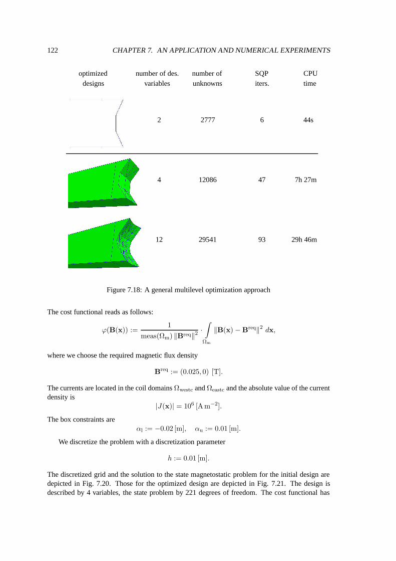
122 CHAPTER 7. AN APPLICATION AND NUMERICAL EXPERIMENTS
optimizeddesigns
number of des.variables
number ofunknowns
SQPiters.
CPUtime
2 2777 6 44s
4 12086 47 7h 27m
12 29541 93 29h 46m
Figure 7.18: A general multilevel optimization approach
The cost functional reads as follows:
ϕ(B(x)) :=1
meas(Ωm) ‖Breq‖2 ·∫
Ωm
‖B(x) −Breq‖2 dx,
where we choose the required magnetic flux density
Breq := (0.025, 0) [T].
The currents are located in the coil domains Ωwestc and Ωeastc and the absolute value of the currentdensity is
|J(x)| = 106 [Am−2].
The box constraints areαl := −0.02 [m], αu := 0.01 [m].
We discretize the problem with a discretization parameter
h := 0.01 [m].
The discretized grid and the solution to the state magnetostatic problem for the initial design aredepicted in Fig. 7.20. Those for the optimized design are depicted in Fig. 7.21. The design isdescribed by 4 variables, the state problem by 221 degrees of freedom. The cost functional has
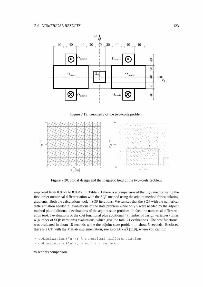
7.4. NUMERICAL RESULTS 123
PSfrag replacements
Ωm ΩeastpΩwestp
Ωeastc
Ωeastc
Ωwestc
Ωwestc
40 4040
4040
40
404040 4020
2020
20
x1
x2
Figure 7.19: Geometry of the two–coils problem
−0.2 −0.1 00
0.05
0.1
PSfrag replacements
x1 [m]
x2[m
]
−0.2 −0.1 00
0.05
0.1
PSfrag replacements
x1 [m]
x2[m
]
Figure 7.20: Initial design and the magnetic field of the two–coils problem
improved from 0.0077 to 0.0042. In Table 7.1 there is a comparison of the SQP method using thefirst–order numerical differentiation with the SQP method using the adjoint method for calculatinggradients. Both the calculations took 4 SQP iterations. We can see that the SQP with the numericaldifferentiation needed 21 evaluations of the state problem while only 5 were needed by the adjointmethod plus additional 4 evaluations of the adjoint state problem. In fact, the numerical differenti-ation took 5 evaluations of the cost functional plus additional 4 (number of design variables) times4 (number of SQP iterations) evaluations, which give the total 21 evaluations. The cost functionalwas evaluated in about 18 seconds while the adjoint state problem in about 5 seconds. Enclosedthere is a CD with the Matlab implementation, see also LUKAS [119], where you can run
> optimization(’n’); % numerical differentiation> optimization(’a’); % adjoint method
to see this comparison.
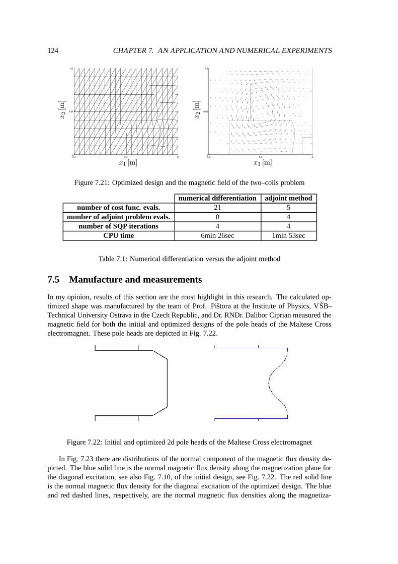
124 CHAPTER 7. AN APPLICATION AND NUMERICAL EXPERIMENTS
−0.2 −0.1 00
0.05
0.1
PSfrag replacements
x1 [m]
x2[m
]
−0.2 −0.1 00
0.05
0.1
PSfrag replacements
x1 [m]
x2[m
]
Figure 7.21: Optimized design and the magnetic field of the two–coils problem
numerical differentiation adjoint methodnumber of cost func. evals. 21 5
number of adjoint problem evals. 0 4number of SQP iterations 4 4
CPU time 6min 26sec 1min 53sec
Table 7.1: Numerical differentiation versus the adjoint method
7.5 Manufacture and measurements
In my opinion, results of this section are the most highlight in this research. The calculated op-timized shape was manufactured by the team of Prof. Pistora at the Institute of Physics, VSB–Technical University Ostrava in the Czech Republic, and Dr. RNDr. Dalibor Ciprian measured themagnetic field for both the initial and optimized designs of the pole heads of the Maltese Crosselectromagnet. These pole heads are depicted in Fig. 7.22.
Figure 7.22: Initial and optimized 2d pole heads of the Maltese Cross electromagnet
In Fig. 7.23 there are distributions of the normal component of the magnetic flux density de-picted. The blue solid line is the normal magnetic flux density along the magnetization plane forthe diagonal excitation, see also Fig. 7.10, of the initial design, see Fig. 7.22. The red solid lineis the normal magnetic flux density for the diagonal excitation of the optimized design. The blueand red dashed lines, respectively, are the normal magnetic flux densities along the magnetiza-
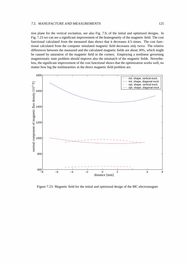
7.5. MANUFACTURE AND MEASUREMENTS 125
tion plane for the vertical excitation, see also Fig. 7.9, of the initial and optimized designs. InFig. 7.23 we can see a significant improvement of the homogeneity of the magnetic field. The costfunctional calculated from the measured data shows that it decreases 4.5–times. The cost func-tional calculated from the computer simulated magnetic field decreases only twice. The relativedifferences between the measured and the calculated magnetic fields are about 30%, which mightbe caused by saturation of the magnetic field in the corners. Employing a nonlinear governingmagnetostatic state problem should improve also the mismatch of the magnetic fields. Neverthe-less, the significant improvement of the cost functional shows that the optimization works well, nomatter how big the nonlinearities in the direct magnetic field problem are.
−8 −6 −4 −2 0 2 6 8600
800
1000
1200
1400
1600
1800init. shape, vertical excit.init. shape, diagonal excit.opt. shape, vertical excit.opt. shape, diagonal excit.
PSfrag replacements
distance [mm]
norm
alco
mpo
nent
ofm
agne
ticfl
uxde
nsity
[10
4T
]
Figure 7.23: Magnetic field for the initial and optimized design of the MC electromagnet

126 CHAPTER 7. AN APPLICATION AND NUMERICAL EXPERIMENTS
Chapter 8
Conclusion
This thesis treated with the shape optimization in both two– and three–dimensional linear magne-tostatics. The aim was to present a complete picture of the mathematical modelling process. Wedealt with both the theoretical and computational aspects and demonstrated them on an applicationbeing of a practical purpose in the research on magnetooptic effects.
Let us summarize the main results obtained in the thesis.
• In Section 3.4 we developed an abstract theory for weak formulations of linear ellipticsecond–order boundary vector–value problems (BVP).
• In Theorem 4.2 we proved the convergence of the solution of the finite element approxi-mation to our abstract BVP while also dealing with an inner approximation of the originaldomain with the Lipschitz boundary by a sequence of domains with polyhedral (or polygo-nal) boundaries.
• In Sections 4.4.1 and 4.4.2 we concretized the abstract framework for the linear Lagrangeand Nedelec elements on triangles or tetrahedra, respectively.
• In Chapter 5 we introduced an abstract shape optimization problem and its finite elementapproximation. We proved both the existence and convergence theorems while they rely onLemma 5.3 and Theorem 4.2, respectively.
• In Section 6.3.4 there is the heart of the thesis. There we developed an efficient implementa-tion of the adjoint method for the first–order sensitivity analysis. We provided also a Matlabimplementation, which is enclosed on the CD.
• In Section 6.4 we introduced a multilevel optimization approach, which is a rather newtechnique. It is the first step towards adaptive optimization algorithms, as they have beenrecently presented in RAMM, MAUTE, AND SCHWARZ [164] and in SCHLEUPEN, MAUTE,AND RAMM [185]. The efficiency of our multilevel optimization approach was documentedon numerical tests in Section 7.4.1.
• Finally, in Chapter 7 we presented a real–life application arising from the research on mag-netooptic effects. We began with the physical description, went through the mathematicalsettings, and ended up with the manufacture of the optimized design and with the discussionof real improvements based on the physical measurements of the magnetic field.
127

128 CHAPTER 8. CONCLUSION
In Chapter 5, we met one serious obstacle, see Remark 5.1, that the standard approximationtheory does not completely cover problems of complex geometries. Namely, it is due to that wecan hardly find a continuous mapping between the shape design nodes and the remaining nodesin the discretization grid. For fine discretizations and large changes in the design shape someelements flip. One possible outcome is in the use of the multilevel optimization techniques whereon the fine grids the difference between the initial and optimized shapes is not that big. Anotheroutcome might be when using composite finite elements that were developed for the treatment withcomplicated geometries in the papers by HACKBUSCH AND SAUTER [79, 80]. It is connected to anidea which was given to me in January 2002 by RNDr. Jan Chleboun, CSc. from the MathematicalInstitute of the Czech Academy of Sciences. The idea is to use a fixed regular grid independentof the geometry and to resolve the fine details of the geometry within special elements that ariseby the intersection of the geometry and the regular grid. This will move all the programmingeffort into the development of such special finite elements instead the shape–to–mesh mapping.We can also avoid this problem by using a boundary element discretization. From its matter, thisis very suited for optimal shape design, as we need to handle only the boundary discretization.Nevertheless, construction of efficient multigrid solvers as well as using the method for nonlineargoverning state problems are still topics of the current research.
Finally, let us draw the further directions of this research. They are mainly focused
• on development and rigorous analysis of the adaptive multilevel techniques in the shapeoptimization,
• on synergies among the inverse and shape optimization problems, namely, on the regular-ization techniques and numerical methods, e.g., the homogenization or level–set methods,
• on common aspects in the topology and shape optimization,
• on development of a user–friendly and well–documented scientific computing software toolfor structural (both shape and topology) optimization,
• and on real–life applications in both electromagnetism and mechanics involving complexgeometries and nonlinearities of the state problem, provided correct mathematical settings,i.e., the existence of a solution at least.

Bibliography
[1] Ansys, http://www.ansys.com.
[2] Fluent, http://www.fluent.com.
[3] J. C. Adam, A. Gourdin-Serveniere, J. C. Nedelec, and P. A. Raviart, Study of an im-plicit scheme for integrating Maxwell’s equations, Comput. Methods Appl. Mech. Eng.22 (1980), 327–346.
[4] R. A. Adams, Sobolev spaces, Academic Press, New York, 1975.
[5] G. Allaire, Homogenization and two–scale convergence, SIAM J. Math. Anal. 23 (1992),1482–1518.
[6] , Shape optimization by the homogenization method, Springer, New York, Berlin,Heidelberg, 2002.
[7] G. Allaire, E. Bonnetier, G. A. Francfort, and F. Jouve, Shape optimization by the homoge-nization method, Numer. Math. 76 (1997), 27–68.
[8] G. Allaire, F. Jouve, and A.-M. Toader, A level–set method for shape optimization, C. R.Acad. Sci. Paris 334 (2002), 1125–1130.
[9] C. Amrouche, C. Bernardi, M. Dauge, and V. Girault, Vector potentials in three–dimensional non–smooth domains, Math. Methods Appl. Sci. 21 (1998), 823–864.
[10] T. Apel and J. Schoberl, Multigrid methods for anisotropic edge refinement, SIAM J. Nu-mer. Anal. 40 (2002), no. 5, 1993–2006.
[11] J. Arora, Introduction to optimum design, McGraw-Hill, New York, 1989.
[12] J. P. Aubin, Approximation of elliptic boundary–value problems, Pure and Applied Mathe-matics, vol. 26, John Wiley & Sons, New York, 1972.
[13] O. Axelsson, Iterative solution methods, Cambridge University Press, 1994.
[14] I. Babuska and A. K. Aziz, Survey lectures on the mathematical foundations of the finiteelement method, The Mathematical Foundations of the Finite Element Method with Appli-cations to Partial Differential Equations, Academic Press, New York and London, 1972.
[15] , On the angle condition in the finite element method, SIAM J. Numer. Anal. 13(1976), 214–226.
129

130 BIBLIOGRAPHY
[16] P. K. Banerjee and R. Butterfield, Boundary element methods in engineering science,McGraw–Hill Book Company, 1981.
[17] N. V. Banichuk, Introduction to optimization of structures, Springer, New York, 1990.
[18] P. Di Barba, P. Navarra, A. Savini, and R. Sikora, Optimum design of iron–core electromag-nets, IEEE Transactions on Magnetics 26 (1990), 646–649.
[19] D. Begis and R. Glowinski, Application de la methode des elements finis a la resolutiond’un probleeme de domaine optimal, Appl. Math. Optimization 2 (1975), 130–169.
[20] M. P. Bendsøe, Optimal shape design as a material distribution problem, Struct. Multidisc.Optim. 1 (1989), 193–202.
[21] , Optimization of structural topology, shape and material, Springer, Berlin, Heidel-berg, 1995.
[22] M. P. Bendsøe and O. Sigmund, Topology optimization. Theory, methods and applications,Springer, Berlin Heidelberg, 2003.
[23] P. T. Boggs and J. W. Tolle, Sequential quadratic programming, Acta Numer. 4 (1995),1–51.
[24] A. D. Borner, Mathematische Modelle fur Optimum Shape Design Probleme in der Magne-tostatik, Ph.D. thesis, Universitat Hamburg, Germany, 1985.
[25] T. Borrvall, Computational topology optimization of elastic continua by design restrictions,Ph.D. thesis, Linkoping University, Sweden, 2000.
[26] A. Bossavit, Computational electromagnetism. Variational formulations, complementarity,edge elements, Orlando, FL: Academic Press, 1998.
[27] D. Braess, Finite elements, Cambridge, 2001.
[28] J. H. Bramble, Multigrid methods, Pitman Research Notes in Mathematics, vol. 294, JohnWiley & Sons, 1993.
[29] J. H. Bramble, J. E. Pasciak, and J. Xu, Parallel multilevel preconditioners, Math. Comput.55 (1990), 1911–1922.
[30] R. B. Brandtstatter, W. Ring, Ch. Magele, and K. R. Richter, Shape design with great geo-metrical deformations using continuously moving finite element nodes, IEEE Transactionson Magnetics 34 (1998), no. 5, 2877–2880.
[31] C. A. Brebbia (ed.), Topics in boundary element research, vol. 6 – electromagnetic applica-tions, Springer, Berlin, 1989.
[32] S. C. Brenner and L. R. Scott, The mathematical theory of finite element methods, Springer,1994.
[33] F. Brezzi and M. Fortin, Mixed and hybrid finite element methods, Springer, New York,1991.

BIBLIOGRAPHY 131
[34] R. A. Brockman, Geometric sensitivity analysis with isoparametric finite elements, Com-mun. Appl. Numer. Methods 3 (1987), 495–499.
[35] D. Bucur and J.-P. Zolesio, Existence and stability of the optimum in shape optimization,ZAMM 76 (1996), no. 2, 77–80.
[36] M. Burger, A level set method for inverse problems, Inverse Probl. 17 (2001), no. 5, 1327–1355.
[37] M. Burger and W. Muhlhuber, Iterative regularization of parameter identification problemsby sequential quadratic programming methods, Inverse Probl. 18 (2002), no. 4, 943–969.
[38] , Numerical approximation of an SQP-type method for parameter identification,SIAM J. Numer. Anal. 40 (2002), no. 5, 1775–1797.
[39] J. Cea, Optimization, theorie et algorithmes, Dunod, Paris, 1971.
[40] J. Cea, S. Garreau, P. Guillaume, and M. Masmoudi, The shape and topological optimiza-tion connections, Comput. Methods Appl. Mech. Eng. 188 (2000), 713–726.
[41] G. Chen and J. Zhou, Boundary element methods, Computational Mathematics and Ap-plications, Academic Press, Harcourt Brave Jovanovich, London, San Diego, New York,1992.
[42] G. Chen, J. Zhou, and R. C. McLean, Boundary element method for shape (domain) op-timization of linear–quadratic elliptic boundary control problem, Boundary Control andVariation. Proceedings of the 5th working conference held in Sophia Antipolis, France, Inc.Lect. Notes Pure Appl. Math., vol. 163, 1994, pp. 27–72.
[43] A. V. Cherkaev, Variational methods for structural optimization, Springer, New York,Berlin, Heidelberg, 2000.
[44] J. Chleboun and R. Makinen, Primal hybrid formulation of an elliptic equation in smoothoptimal shape problems, Adv. Math. Sci. Appl. 5 (1995), no. 1, 139–162.
[45] P. Ciarlet, The finite element method for elliptic problems, North–Holland, 1978.
[46] P. G. Ciarlet and J. Lions (eds.), Handbook of numerical analysis, North–Holland, Amster-dam, 1989.
[47] D. Cioranescu and P. Donato, An introduction to homogenization, Oxford Lect. Series Math.Appl., vol. 17, Oxford University Press, 1999.
[48] F. H. Clarke, Nonsmooth analysis and optimization, Wiley & Sons, 1983.
[49] A. R. Conn, N. I. M. Gould, and P. L. Toint, Trust–region methods, MPS–SIAM Series onOptimization, vol. 1, SIAM, Philadelphia, 2000.
[50] M. Costabel and M. Dauge, Singularities of Maxwell’s equations on polyhedral domains,Numerics and applications of differential and integral equations (M. Bach, C. Constanda,and G. C. Hsiao et. al., eds.), Pitman Research Notes in Mathematics Series, vol. 379,Harlow: Adison Wesley Longman, 1998.
132 BIBLIOGRAPHY
[51] R. Courant and D. Hilbert, Methods of mathematical physics, Interscience Publishers, NewYork, 1962.
[52] W. C. Davidon, Variable metric method for minimization, Technical report ANL–5990 (re-vised), Argonne National Laboratory, 1959.
[53] , Variable metric method for minimization, SIAM J. Optim. 1 (1991), 1–17.
[54] M. C. Delfour and J.-P. Zolesio, Shape and geometries: Analysis, differential calculus, andoptimization, Advances in Design and Control, vol. 4, SIAM, 2001.
[55] J. E. Dennis and R. B. Schnabel, Numerical methods for unconstrained optimization andnonlinear equations, Prentice Hall, 1983.
[56] P. Doktor, On the density of smooth functions in certain subspaces of Sobolev spaces, Com-ment. Math. Univ. Carol. 14 (1973), 609–622.
[57] Z. Dostal, Linear algebra, Lecture Notes, VSB–Technical University of Ostrava, 2000, inCzech.
[58] H. W. Engl, M. Hanke, and A. Neubauer, Regularization of inverse problems, Kluwer Aca-demic Publishers, Dordrecht, Boston, London, 1996.
[59] G. E. Farin, Curves and surfaces for computer-aided geometric design: A practical guide,Academic Press, 1996.
[60] R. P. Feynman, R. B. Leightona, and M. Sands, The Feynman lectures on physics, vol. 3,Addison–Wesley, 1966.
[61] R. Fletcher, Practical optimization methods, 2nd edition, Wiley & Sons, 1987.
[62] , An optimal positive definite update for sparse Hessian matrices, SIAM J. Optim.5 (1995), 192–218.
[63] R. Fletcher and C. M. Reeves, Function minimization by conjugate gradients, Comput. J. 7(1964), 149–154.
[64] J. Francu, Monotone operators. A survey directed to applications to differential equations,Appl. Math. Praha 35 (1990), 257–301.
[65] P. L. George, Automatic mesh generation, John Wiley & Sons, 1993.
[66] P. Gill, W. Murray, and M. Wright, Practical optimization, Academic Press, 1981.
[67] V. Girault and P. Raviart, Finite element methods for Navier–Stokes equations, Springer,Berlin, 1986.
[68] R. Glowinski, Numerical methods for nonlinear variational problems, Springer, New York,1984.
[69] G. H. Golub and C. F. van Loan, Matrix computation, 2nd ed., Johns Hopkins Series in theMathematical Sciences, The Johns Hopkins University Press, 1989.
[70] A. Griewank, Evaluating derivatives, principles and techniques of algorithmic differentia-tion, Frontiers in Applied Mathematics, vol. 19, SIAM, Philadelphia, 2000.
BIBLIOGRAPHY 133
[71] C. Grossmann and H.-G. Ross, Numerik partieller Differentialgleichungen, Teubner Studi-enbucher, Stuttgart, 1992.
[72] C. Grossmann and J. Terno, Numerik der Optimierung, 2nd ed., Teubner Studienbucher,Stuttgart, 1997.
[73] G. Haase, M. Kuhn, U. Langer, S. Reitzinger, and J. Schoberl, Parallel Maxwell solvers,Scientific computing in electrical engineering (Ursula van Rienen, Michael Gunther, andDirk Hecht, eds.), Lect. Notes Comput. Sci. Eng., vol. 18, 2001, pp. 71–78.
[74] G. Haase and U. Langer, On the use of multigrid preconditioners in the domain decomposi-tion method, Parallel algorithms for partial differential equations, Proc. 6th GAMM-Semin.,Notes Numer. Fluid Mech., vol. 31, 1991, pp. 101–110.
[75] G. Haase, U. Langer, A. Meyer, and S.V. Nepomnyaschikh, Hierarchical extension oper-ators and local multigrid methods in domain decomposition preconditioners, East West J.Numer. Math. 31 (1994), no. 4–5, 269–272.
[76] G. Haase, U. Langer, S. Reitzinger, and J. Schoberl, Algebraic multigrid methods based onelement preconditioning, Int. J. Comput. Math. 78 (2001), no. 4, 575–598.
[77] G. Haase and E. Lindner, Advanced solving techniques in optimization of machine compo-nents, Comput. Assist. Mech. Eng. Sci. 6 (1999), no. 3, 337–343.
[78] W. Hackbusch, Multi–grid methods and applications, Springer, Berlin, 1985.
[79] W. Hackbusch and S. A. Sauter, Composite finite elements for problems containing smallgeometric details - part II: Implementation and numerical results, Comput. Vis. Sci. 1(1997), 15–25.
[80] , Composite finite elements for the approximation of PDEs on domains with com-plicated micro–structures, Numer. Math. 75 (1997), 447–472.
[81] W. W. Hager, D. W. Hearn, and P. M. Pardalos (eds.), Large scale optimization, KluwerAcademic Publishers, Dordrecht, 1994.
[82] J. S. Hansen, Z. S. Liu, and N. Olhoff, Shape sensitivity analysis using a fixed basis functionfinite element approach, Struct. Multidisc. Optim. 21 (2001), 177–196.
[83] J. Haslinger and R. A. E. Makinen, Introduction to shape optimization. Theory, approx-imation, and computation, Advances in Design and Control, vol. 7, SIAM, Philadelphia,2003.
[84] J. Haslinger, M. Miettinen, and D. Panagiotopoulos, Finite element method for hemivari-ational inequalities. Theory, methods and applications, Nonconvex Optimization and itsApplications, vol. 35, Kluwer Academic Publishers, Dordrecht, 1999.
[85] J. Haslinger and P. Neittaanmaki, Finite element approximation for optimal shape, materialand topology design, 2nd ed., John Wiley & Sons Ltd., Chinchester, 1997.
[86] E. J. Haug, K. K. Choi, and V. Komkov, Sensitivity analysis in structural design, Mathe-matics in Science and Engineering, vol. 177, Academic Press, 1986.
134 BIBLIOGRAPHY
[87] H. A. Haus and J. R. Melcher, Electromagnetic fields and energy, Englewood Cliffs, Pren-tice Hall, 1989.
[88] M. R. Hestensen, Optimization theory, John Wiley & Sons, 1975.
[89] , Conjugate direction methods in optimization, Springer, 1980.
[90] M. R. Hestensen and E. Stiefel, Methods of conjugate gradients for solving linear systems,J. Res. Natl. Inst. Stand. Technol. 49 (1952), 409–436.
[91] R. Hiptmair, Multilevel preconditioning for mixed problems in three dimensions, Ph.D. the-sis, University of Augsburg, Germany, 1996.
[92] , Canonical construction of finite elements, Math. Comput. 68 (1999), 1325–1346.
[93] , Finite elements in computational electromagnetism, Acta Numer. (2002), 237–339.
[94] R. Hiptmair and C. Schwab, Natural boundary element methods for the electric field inte-gral equation on polyhedra, SIAM J. Numer. Anal. 40 (2002), no. 1, 66–86.
[95] I. Hlavacek, J. Haslinger, J. Necas, and J. Lovısek, Numerical solution of variational in-equalities, Springer, Berlin, 1988.
[96] R. H. W. Hoppe, S. I. Petrova, and V. H. Schulz, Numerical analysis and applications– topology optimization of conductive media described by Maxwell’s equations, LectureNotes Comput. Sci. (1988), 414–422.
[97] , 3d structural optimization in electromagnetics, Proceedings of Domain Decompo-sition Methods and Applications (Lyon, Oct. 9–12, 2000) (M. Garbey et al., ed.), 2001.
[98] T. J. R. Hughes, The finite element method, Prentice–Hall, Englewood Cliffs, New Jersey,1987.
[99] N. Ida and J. P. A. Bastos, Electromagnetics and calculation of fields, Springer, 1997.
[100] J. B. Jacobsen, N. Olhoff, and E. Rønholt, Generalized shape optimization of three–dimensional structures using materials with optimum microstuctures, Mechanics of Ma-terials 28 (1998), no. 1–4, 207–225.
[101] C. Johnson, Numerical solution of partial differential equations by the finite elementmethod, Cambridge University Press, 1990.
[102] M. Jung and U. Langer, Applications of multilevel methods to practical problems, Surv.Math. Ind. 1 (1991), no. 3, 217–257.
[103] , Methode der finiten Elemente fur Ingenieure: Eine Einfuhrung in die numerischenGrundlagen und Computersimulation, Teubner, Stuttgart, 2001.
[104] J. Kacur, J. Necas, J. Polak, and J. Soucek, Convergence of a method for solving the mag-netostatic field in nonlinear media, Appl. Math. Praha 13 (1968), 456–465.
[105] A. M. Kalamkarov and A. G. Kolpakov, Analysis, design and optimization of compositestructures, John Wiley & Sons, New York; London; Sydney, 1997.

BIBLIOGRAPHY 135
[106] M. Kaltenbacher, H. Landes, R. Lerch, and F. Lindinger, A finite–element / boundary–element method for the simulation of coupled electrostatic–mechanical systems, J. PhysiqueIII 7 (1997), 1975–1982.
[107] B. Kawohl, O. Pironneau, L. Tartar, and J.-P. Zolesio (eds.), Optimal shape design, LectureNotes in Mathematics, vol. 1740, Springer, Berlin, New York, Heidelberg, 2000.
[108] N. Kikuchi, Finite element methods in mechanics, Cambridge University Press, 1986.
[109] A. Kirsch, An introduction to the mathematical theory of inverse problems, Springer Seriesin Applied Mathematical Sciences, vol. 120, Springer, Berlin, 1996.
[110] E. Kita and H. Tanie, Topology and shape optimization of continuum structures using GAand BEM, Struct. Multidisc. Optim. 17 (1999), no. 2–3, 130–139.
[111] I. Kopriva, D. Hrabovsky, K. Postava, D. Ciprian, and J. Pistora, Anisotropy of the quadraticmagneto-optical effects in a cubic crystal, Proceedings of SPIE, vol. 4016, 2000, pp. 54–59.
[112] A. Kost, Numerische Methode in der Berechnung elektromagnetischer Felder, Springer,Berlin, Heidelberg, New York, 1995.
[113] M. Krızek, On the maximum angle condition for linear tetrahedral elements, SIAM J. Nu-mer. Anal. 29 (1992), 513–520.
[114] M. Krızek and P. Neittaanmaki, On superconvergence techniques, Acta Appl. Math. 9(1987), 175–198.
[115] M. Krızek and P. Neittaanmaki, Mathematical and numerical modelling in electrical engi-neering, Kluwer Academic Publishers, Dordrecht, 1996.
[116] A. Kufner, O. John, and S. Fucık, Function spaces, Academia, Prague, 1977.
[117] M. Kuhn, U. Langer, and J. Schoberl, Scientific computing tools for 3d magnetic field prob-lems, The Mathematics of Finite Elements and Applications (MAFELAP X) (2000), 239–259.
[118] E. Laporte and P. Le Tallec, Numerical methods in sensitivity analysis and shape opti-mization, Modeling and Simulation in Science, Engineering and Technology, Birkhauser,Boston, 2003.
[119] D. Lukas, 2–d shape optimization for magnetostatics, Tutorial for a students project at theconference Industrial Mathematics and Mathematical Modelling (IMAMM) 2003, Roznovpod Radhostem, Czech Republic, http://lukas.am.vsb.cz/Teaching/IMAMM2003/.
[120] , On solution to an optimal shape design problem in 3-dimensional magnetostatics,Appl. Math. Praha, Submitted.
[121] , On the road – between Sobolev spaces and a manufacture of homogeneous elec-tromagnets, Transactions of the VSB-TU of Ostrava, vol. 2, VSB–TU Ostrava, To appear.
[122] , Shape optimization of homogeneous electromagnets, Tech. report, Special-forschungsbereich SFB F013, University Linz, 2000.
136 BIBLIOGRAPHY
[123] , Shape optimization of homogeneous electromagnets, Scientific Computing inElectrical Engineering (Ursula van Rienen, Michael Gunther, and Dirk Hecht, eds.), Lect.Notes Comp. Sci. Eng., vol. 18, Springer, 2001, pp. 145–152.
[124] D. Lukas, I. Kopriva, D. Ciprian, and J. Pistora, Shape optimization of homogeneous electro-magnets and their application to measurements of magnetooptic effects, Records of COM-PUMAG 2001, vol. 4, 2001, pp. 156–157.
[125] D. Lukas, W. Muhlhuber, and M. Kuhn, An object-oriented library for the shape optimiza-tion problems governed by systems of linear elliptic partial differential equations, Transac-tions of the VSB-TU of Ostrava, vol. 1, VSB–TU Ostrava, 2001, pp. 115–128.
[126] D. Lukas, J. Vlcek, Z. Hytka, and Z. Dostal, Optimization of dislocation of magnets in amagnetic separator, Transactions of the VSB-TU of Ostrava, Electrical Engineering Series,vol. 1, VSB–TU Ostrava, 1999, pp. 1–12.
[127] D. Lukas, Shape optimization of a magnetic separator, Master’s thesis, VSB - TechnicalUniversity of Ostrava, Czech Republic, 1999, In Czech.
[128] D. Lukas, Multilevel solvers for 3–dimensional optimal shape design with an application tomagnetostatics, Book of Abstracts of the 9th International Symposium on Microwave andOptical Technology, Ostrava, 2003, p. 121.
[129] J. Lukes and J. Maly, Measure and integral, MATFYZPRESS, 1995.
[130] M. Makela and P. Neittaanmaki, Nonsmooth optimization: Analysis and algorithms withapplications to the optimal control, World Scientific Publishing Company, Singapore, 1992.
[131] R. Makinen, Finite element design sensitivity analysis for nonlinear potential problems,Commun. Appl. Numer. Methods 6 (1986), 343–350.
[132] A. Marrocco and O. Pironneau, Optimum design with Lagrangian finite elements: Designof an electromagnet, Comput. Methods Appl. Mech. Eng. 15 (1978), 277–308.
[133] I. D. Mayergoyz, Mathematical models of hysteresis, Springer, Berlin, 1991.
[134] V. G. Mazya, Sobolev spaces, Springer, Berlin, 1985.
[135] B. Mohammadi and O. Pironneau, Applied shape optimization for fluids, Oxford UniversityPress, Oxford, 2001.
[136] P. Monk, Analysis of a finite element method for Maxwell’s equations, SIAM J. Numer.Anal. 29 (1992), 714–729.
[137] , A comparison of three mixed methods for the time dependent Maxwell’s equations,SIAM J. Sci. Statist. Comput. 13 (1992), 1097–1122.
[138] , A finite elemeny method for approximating the time–harmonic Maxwell’s equa-tions, Numer. Math. 63 (1992), 243–261.
[139] W. Muhlhuber, Efficient solvers for optimal design problems with PDE constraints, Ph.D.thesis, Johannes Kepler University Linz, Austria, 2002.
BIBLIOGRAPHY 137
[140] F. Murat and J. Simon, Studies on optimal shape design problems, Lecture Notes in Com-putational Science, vol. 41, Springer, Berlin, 1976.
[141] J. Necas, Les methodes directes en theorie des equations elliptiques, Academia, Prague,1967.
[142] J. C. Nedelec, Mixed finite elements in R3, Numer. Math. 35 (1980), 315–341.
[143] , A new family of mixed finite elements in R3, Numer. Math. 50 (1986), 57–81.
[144] P. Neittaanmaki, M. Rudnicki, and A. Savini, Inverse problems and optimal design in elec-tricity and magnetism, Oxford University Press, 1995.
[145] P. Neittaanmaki and K. Salmenjoki, Sensitivity analysis for optimal shape design problems,Struct. Multidisc. Optim. 1 (1989), 241–251.
[146] P. Neittaanmaki and J. Saranen, Finite element approximation of electromagnetic fields inthe three dimensional space, Numer. Funct. Anal. Optim. 2 (1981), 487–506.
[147] , Finite element approximations of vector fields given by curl and divergence, Math.Methods Appl. Sci. 3 (1981), 328–335.
[148] J. Nocedal and S. J. Wright, Numerical optimization, Springer, 1999.
[149] J. T. Oden and L. F. Demkowicz, Applied functional analysis, CRC Press, 1996.
[150] J. T. Oden and J. N. Reddy, An introduction to the mathematical theory of finite elements,John Wiley & Sons, 1976.
[151] N. Olhoff, Multicriterion structural optimization via bound formulation and mathematicalprogramming, Struct. Multidisc. Optim. 1 (1989), 11–17.
[152] N. Olhoff and J. E. Taylor, On structural optimization, J. Appl. Math. 50 (1983), no. 4,1139–1151.
[153] A. R. Parkinson and R. J. Balling, The OptdesX design optimization software, Struct. Mul-tidisc. Optim. 23 (2002), 127–139.
[154] P. Pedersen (ed.), Optimal design with advanced materials, Elsevier, Amsterdam, TheNetherlands, 1993.
[155] G. H. Peichl and W. Ring, Optimization of the shape of an electromagnet: Regularity re-sults, Adv. Math. Sci. and Appl. 8 (1998), 997–1014.
[156] , Asymptotic commutativity of differentiation and discretization in shape optimiza-tion, Math. and Comput. Modelling 29 (1999), 19–37.
[157] J. Petersson, On continuity of the design–to–state mappings for trusses with variable topol-ogy, Int. J. Eng. Sci. 39 (2001), no. 10, 1119–1141.
[158] J. Petersson and J. Haslinger, An approximation theory for optimum sheets in unilateralcontact, Q. Appl. Math. 56 (1998), no. 2, 309–332.
[159] O. Pironneau, Optimal shape design for elliptic systems, Springer Series in ComputationalPhysics, Springer, New-York, 1984.
138 BIBLIOGRAPHY
[160] J. Pistora, K. Postava, and R. Sebesta, Optical guided modes in sandwiches with ultrathinmetallic films, Journal of Magnetism and Magnetic Materials 198–199 (1999), 683–685.
[161] E. Polak, Computational methods in optimization. A unified approach, Academic Press,New York, 1971.
[162] E. Polak and G. Ribiere, Note sur la convergence de methodes de directions conjuguees,Rev. Fr. Inf. Rech. Oper. 16 (1969), 35–43.
[163] A. Ralston, Zaklady numericke matematiky (Fundamentals of numerical mathematics),Academia Praha, 1978.
[164] E. Ramm, K. Maute, and S. Schwarz, Adaptive topology and shape optimization, 1998,http://citeseer.nj.nec.com/ramm98adaptive.html.
[165] J. Rasmussen, M. Damsgaard, S. T. Christensen, and E. Surma, Design optimization withrespect to ergonomic properties, Struct. Multidisc. Optim. 24 (2002), 89–97.
[166] J. Rasmussen, E. Lund, T. Birker, and N. Olhoff, The CAOS system, Int. Ser. Numer. Math.110 (1993), 75–96.
[167] P. A. Raviart and J. M. Thomas, A mixed finite element method for second order ellipticproblems, Lect. Notes Math. 606 (1977), 292–315.
[168] S. Reitzinger, PEBBLES – user’s guide, SFB ”Numerical and Symbolic Scientific Comput-ing”, http://www.sfb013.uni-linz.ac.at.
[169] , Algebraic multigrid methods for large scale finite element equations, Ph.D. thesis,Johannes Kepler University Linz, Austria, 2001.
[170] K. Rektorys, Survey of applicable mathematics, Kluwer, Amsterdam, 1994.
[171] A. Rietz and J. Petersson, Simultaneous shape and thickness optimization, Struct. Multidisc.Optim. 23 (2001), no. 1, 14–23.
[172] W. Ritz, Uber eine neue Methode zur Losung gewisser Variationsprobleme der mathema-tischen Physik, J. Reine Angew. Math. 135 (1909), 1–61.
[173] G. I. N. Rozvany (ed.), Shape and lay–out optimization of structural systems and optimalitycriteria methods, CISM Lecture Notes no. 325, Springer, Wien, 1992.
[174] G. I. N. Rozvany (ed.), Optimization of large structural systems, Kluwer Academic Pub-lishers, Dordrecht, The Netherlands, 1993.
[175] , Aims, scope, methods, history and unified terminology of computer–aided topologyoptimization in structural mechanics, Struct. Multidisc. Optim. 21 (2001), 90–108.
[176] W. Rudin, Real and complex analysis, McGraw Hill, New York, 1966.
[177] , Functional analysis, McGraw Hill, New York, 1973.
[178] , Principles of mathematical analysis, 3rd ed., International Series in Pure and Ap-plied Mathematics, McGraw-Hill Book Company, 1976.

BIBLIOGRAPHY 139
[179] Y. Saad, Iterative methods for sparse linear systems, PWS, 1996, 2nd edition available athttp://www.cs.umn.edu/˜saad/books.html.
[180] M. Save and W. Prager (eds.), Structural optimization, vol. 1, optimality criteria, PlenumPress, New York, 1985.
[181] M. Save and W. Prager (eds.), Structural optimization, vol. 2, mathematical optimization,Plenum Press, New York, 1990.
[182] O. Scherzer, An iterative multi level algorithm for solving nonlinear ill–posed problems,Numer. Math. 80 (1998), 579–600.
[183] M. Schinnerl, U. Langer, and R. Lerch, Multigrid simulation of electromagnetic actuators,ZAMM, Z. Angew. Math. Mech. 81 (2001), no. 3, 729–730.
[184] M. Schinnerl, J. Schoberl, M. Kaltenbacher, U. Langer, and R. Lerch, Multigrid methods forthe fast numerical simulation of coupled magnetomechanical systems, ZAMM Z. Angew.Math. Mech. 80 (2000), no. 1, 117–120.
[185] A. Schleupen, K. Maute, and E. Ramm, Adaptive FE–procedures in shape optimization,Struct. Multidisc. Optim. 19 (2000), 282–302.
[186] J. Schoberl, NETGEN - An advancing front 2D/3D-mesh generator based on abstract rules,Comput. Vis. Sci. (1997), 41–52.
[187] C. Schwab, p– and hp– finite element methods: Theory and applications to solid and fluidmechanics, Oxford University Press, 1998.
[188] J. Sethian and A. Wiegmann, Structural boundary design via level set and immersed inter-face methods, J. Comp. Phys. 163 (2000), 489–528.
[189] R. E. Showalter, Hilbert space methods for partial differential equations, Pitman, London,San Francisco, 1977.
[190] O. Sigmund and J. Petersson, Numerical instabilities in topology optimization: A surveyon procedures dealing with chechkerboards, mesh–dependencies and local minima, Struct.Multidisc. Optim. 16 (1998), no. 1, 68–75.
[191] C. A. C. Silva and M. L. Bittencourt, An object–oriented structural optimization program,Struct. Multidisc. Optim. 20 (2000), 154–166.
[192] P. P. Silvester and R. L. Ferrari, Finite elements for electrical engineers, Cambridge Uni-versity Press, 1983.
[193] J. Simon, Differentiation with respect to the domain in boundary value problems, Numer.Funct. Anal. Optimization 2 (1980), 649–687.
[194] S. L. Sobolev, Applications of functional analysis in mathematical physics, American Math-ematical Society, Providence, 1963.
[195] J. Sokolowski and A. Zochowski, On the topological derivative in shape optimization,SIAM J. Control Optimization 37 (1999), 1251–1272.
140 BIBLIOGRAPHY
[196] J. Sokolowski and J.-P. Zolesio, Introduction to shape optimization, Springer Series in Com-putational Mathematics, no. 16, Springer, Berlin, 1992.
[197] L. Solymar, Lectures on electromagnetic theory, Oxford University Press, 1987.
[198] W. Stadler, Non–existence of solutions in optimal structural design, Optim. Control Appl.Methods 7 (1986), 243–258.
[199] C. W. Steele, Numerical computation of electric and magnetic fields, Van Nostrand ReynoldCo., New York, 1987.
[200] G. Strang and G. J. Fix, An analysis of the finite element method, Prentice-Hall, 1973.
[201] J. A. Stratton, Electromagnetic theory, Mc Graw–Hill Book Co., Inc., New York, 1941.
[202] K. Suzuki and N. Kikuchi, A homogenization method for shape and topology optimization,Comput. Methods Appl. Mech. Eng. 93 (1991), no. 3, 291–318.
[203] K. Svanberg, The method of moving asymptotes – a new method for structural optimization,Int. J. Numer. Methods Eng. 24 (1987), 359–373.
[204] , A class of globally convergent optimization methods based on conservative convexseparable approximations, SIAM J. Optim. 12 (2002), no. 2, 555–573.
[205] B. Szabo and I. Babuska, Finite element analysis, John Wiley & Sons, 1991.
[206] N. Takahashi, Optimization of die press model, Proceedings of the TEAM Workshop in theSixth Round (Okayama, Japan), March 1996.
[207] P.-S. Tang and K.-H. Chang, Integration of topology and shape optimization for design ofstructural components, Struct. Multidisc. Optim. 22 (2001), 65–82.
[208] The MathWorks, Inc., Matlab user manual, 1993.
[209] H. Thomas, L. Zhou, and U. Schramm, Issues of commercial optimization software devel-opment, Struct. Multidisc. Optim. 23 (2002), no. 2, 97–110.
[210] D. Tscherniak and O. Sigmund, A web–based topology optimization program, Struct. Mul-tidisc. Optim. 22 (2001), no. 3, 179–187.
[211] U. van Rienen, Numerical methods in computational electrodynamics. linear systems inpractical applications, Lecture Notes in Computational Science and Engineering, vol. 12,Springer, Berlin, 2001.
[212] K. Washizu, Variational methods in elasticity and plasticity, Pergamon, Oxford, GreatBritain, 1983.
[213] Y. M. Xie and G. P. Steven, Evolutionary structural optimization, Springer, Berlin, 1997.
[214] J. Yoo and N. Kikuchi, Topology optimization in magnetic fields using the homogenizationdesign method, Int. J. Numer. Meth. Eng. 48 (2000), 1463–1479.
[215] K. Yuge, N. Iwai, and N. Kikuchi, Optimization of 2–d structures subjected to nonlineardeformations using the homogenization method, Struct. Multidisc. Optim. 17 (1999), no. 4,286–298.
BIBLIOGRAPHY 141
[216] K. Yuge and N. Kikuchi, Optimization of a frame structure subjected to a plastic deforma-tion, Struct. Multidisc. Optim. 10 (1995), no. 3–4, 197–208.
[217] O. C. Zienkiewicz, The finite element method in engineering science, London etc.:McGraw-Hill XIV, 1971.
[218] O. C. Zienkiewicz and R. L. Taylor, The finite element method (parts 1–3), ButterworthHeinemann, Oxford, 2000.
[219] M. Zlamal, On the finite element method, Numer. Math. 12 (1968), 394–409.
[220] J.-P. Zolesio, The material derivative (or speed) method for shape optimization, Optimiza-tion of Distributed Parameter Structures, Part II (E. J. Haug and J. Cea, eds.), NATO Adv.Study Inst., 1981, pp. 1089–1151.
[221] G. Zoutendijk, Methods of feasible directions, Elsevier, Amsterdam, 1960.
[222] J. Zowe, M. Kocvara, and M. P. Bendsøe, Free material optimization via mathematicalprogramming, Math. Program. 79 (1997), no. 1–3, Ser. B, 445–466.
[223] A. K. Zvedin and V. A. Kotov, Modern magnetooptics and magnetooptical materials, Insti-tute of Physics Publishing Bristol and Philadelphia, 1997.

142 BIBLIOGRAPHY
Curriculum vitae
Personal data
Name: Ing. Dalibor LukasDate and place of birth: June 10, 1976 in Ostrava, Czech Republic
Education
1990 - 1994: High Electrotechnical School (SPSE) in Havırov, Czech Republic1994 - 1999: studies in Informatics and Applied Mathematics at the VSB–
Technical University of Ostrava, Czech Republicsince November 1999: Ph.D. student in Informatics and Applied Mathematics at the
VSB–Technical University of Ostrava, Czech Republic
Career history
August 1996: programmer at the company Q-gir in Ostrava, Czech RepublicApril–July 1999: programmer at the company Voest-Alpine Industrienlangebau
GmbH in Leoben, AustriaApril 2000–March 2001: research fellow at the Spezialforschungsbereich SFB013 “Nu-
merical and Symbolic Scientific Computing”, Project F1309 “Hi-erarchical Optimal Design Methods”, University Linz, Austria
December 2002–May 2003: research assistant at the Department of Applied Mathematics,VSB–Technical University of Ostrava, Czech Republic
since June 2003: research fellow at the SFB013 “Numerical and Symbolic Scien-tific Computing”, Project F1309 “Multilevel Solvers for LargeScale Discretized Optimization Problems”, University Linz, Aus-tria
Publications
M.Sc. thesis [127], 1 article to appear in a refereed journal [120], 2 articles in refereed conferenceproceedings [123, 124], 4 refereed technical reports [121, 122, 125, 126], 5 contributed talks and3 posters at international conferences, and 1 tutorial of a student conference project [119]
Research interests
Shape optimization, finite element method, mathematical modelling, scientific computing, mag-netostatics
For more information see: http://lukas.am.vsb.cz
143