Optimal Sale Across Venuesand Auctions with a Buy-Now Option∗

Subir BoseUniversity of Leicester, Leicester, UK

Arup DaripaBirkbeck College, London University

Bloomsbury, London, UK

Original Version: January 2007, Revised version: January 2008

Abstract: We characterize the optimal selling mechanism for a seller who faces demand de-

marcated by a high and a low end and who can access an (online) auction site (by paying

an access cost) in addition to using his own store that can be used as a posted price selling

venue. We first solve for the optimal mechanism of a direct revelation game in which there

is no venue-restriction constraint. We find that the direct optimal mechanism must necessar-

ily incorporate a certain kind of pooling. We then show that even with the venue constraint,

the seller can use a two stage indirect mechanism that implements the allocation rule from the

optimal direct mechanism, and uses the venues in an optimal fashion. The first stage of the in-

direct mechanism is a posted price at the store. If the object is not sold, we move to stage two,

which involves an auction at the auction site. A feature of this auction is a buy-now option

which is essential for implementing the pooling feature of the optimal direct mechanism. We

also show that the buy-now option in the optimal mechanism is of a “temporary” variety, and

that a “permanent” buy-now option, in contrast, cannot implement the optimal mechanism.

Auctions with a temporary buy-now option are in widespread use on eBay.

KEYWORDS: Optimal Auction, eBay Auctions, Temporary Buy-Now Option, Permanent Buy-

Now Option, Heterogeneous Sales Venues, Posted Price, Price Discrimination

JEL CLASSIFICATION: D44

∗We thank the Associate Editor, George Deltas, for his insightful comments. We also thank seminar

participants at the University of Basel and the SAET conference 2007.

1 INTRODUCTION

Low transactions cost of trading on the Internet has led to a tremendous growth in the

scope of auctions. Moreover, the advent of listing sites such as eBay and Yahoo! have

made it very easy to sell an object through an auction and provide access to a large pool

of buyers. Initially, most of the goods sold through online auctions were collectables(2).

Increasingly, however, goods traditionally sold at posted prices (through bricks-and-

mortar stores and web sites) are being offered also through online auctions. A large

part of the standard goods sold through auctions are overstock items from wholesalers

and standard retailers. Overstock.com, which describes itself as “an Internet leader for

name-brands at clearance prices,” sells items through both posted prices and auctions.

IBM has launched its own eBay auctions to sell discontinued products. Other compa-

nies such as Dell, HP, Gateway, and Sears, who have well established posted price sales

channels, have opened up eBay stores to sell overstock items and refurbished systems

through auctions. (3)

Many sellers sell through conventional stores making use of a posted price. Evidently,

such stores might increase revenue if they could arrange an auction, but typically hold-

ing an auction at such venues is very costly, ruling it out as a practical option. It is of

course much cheaper to set up auctions online, and the advent of such auctions in

recent years has given sellers access to a sales channel that augments existing posted

price channels, allowing the sellers to expand their market base.

This role of auctions as an additional sales channel is the focus in our paper. Specifi-

cally, we characterize the optimal sales mechanism in an environment where a seller,

facing demand that has a clearly demarcated high and low end, can access a sales

venue restricted to posted prices, and, at a small cost, access another venue to use an

auction that the seller designs. Our results show that in the optimal selling mechanism,

the seller uses different venues to target the different ends of the market: the good is

sold to the “high-end” buyers through a posted price and if the good is not sold at the

posted price, to “ lower-end” buyers through an auction that includes a non-standard

feature in the form of a buy-now option. An important insight from our analysis is

(2)See Lucking-Reiley (2000).(3)Also see Miller (2005) for a variety of examples.

1

that since the optimal design involves second degree price discrimination across indi-

vidual selling mechanisms, individual components of the overall optimal mechanism

may seem suboptimal if considered in isolation. Our analysis also provides a novel

theoretical justification for auctions with buy-now options by showing that they form

part of the optimal selling mechanism.(4) Note also that even though our formal model

has a single unit, the intuition should carry over to more general frameworks incorpo-

rating multiple items as long as the stochastic nature of the demand implies that items

are sometimes left unsold at the (posted price) store. Taking a broader perspective, our

work connects the literature on optimal auctions to the industrial literature on opti-

mal pricing by considering the optimal auction design exercise in a scenario where an

auction is part of a bigger set of sales methods used by a seller.

We model the environment as follows. There is a seller who owns a store (we refer to

this as selling venue 1) which uses a posted price to sell the object. A second selling

venue is an (online) auction site, which the seller can access at some cost c > 0.(5)

The seller can choose the posted price and the auction format. To capture the high

and low ends of the demand side we model the distribution from which buyers draw

valuations as follows: with probability µ a buyer has value vh for the object, an event

that can be interpreted as the “ high end” of the market. With probability (1 − µ) the

buyer can have a range of possible values all of which are less than vh. Specifically,

with probability (1− µ) a buyer’s value is drawn from the interval [v, v] where v < vh.

We make the standard assumption that a buyer’s value is private information. Given

this environment, we ask what the optimal selling strategy for the seller is and use

techniques from the mechanism design literature to answer this question.(6)

(4)The literature typically describes environments where such auctions are superior only to certain

standard auctions (usually the English auction). As far as we know, we are the first to show that these

auctions can arise as part of the optimal mechanism in certain environments. We discuss buy-now options

at greater length later in the introduction.(5)For example, the sellers using eBay have to pay a listing fee as well as a percentage of the final selling

price to eBay. Similar charges are also applied by other auction platforms. However, we emphasize that

here c is an additional cost of accessing the auction site. In order to not carry unnecessary notations, we

assume that the cost of accessing the store that the seller owns is zero (i.e. any cost incurred is already

sunk) and the cost of accessing the auction site is c > 0.(6)See the comments at the end of this subsection for our choice of the atom to represent the high-end

of the market.

2

Instead of solving for the seller’s optimal strategy directly, we follow an indirect ap-

proach that we find useful and instructive. We first consider a direct revelation game

ignoring any venue restrictions. In other words, we first analyze the seller’s problem

as if it was a standard mechanism design exercise. We then consider the problem in-

corporating the venue restrictions.

Let us first describe the direct revelation game. Note that we have a non-regular dis-

tribution which cannot be addressed by standard methods. The presence of the gap

(zero density over some range) and the atom makes it fall outside the analysis of

Myerson (1981). We therefore derive the optimal mechanism directly. However, as

we explain later (section 3.5), the environment we consider can be thought of as the

limit of a non-regular case of Myerson. Thus, an additional (minor) contribution of our

work is the verification that the optimal mechanism has no discontinuity at the limit.

We characterize the optimal direct mechanism and show that this involves a cutoff

v∗ < v, such that types above this cutoff are pooled. The intuition is as follows. The

payment that can be extracted from type vh depends on the information rent it can

earn which in turn depends on its payoff when reporting some type other than vh.

Extracting the optimal amount of surplus from type vh while maintaining its incentive

constraint requires “downgrading” its chances of winning the object if it reports its

type untruthfully. This is what the pooling accomplishes. The allocation rule is efficient

over the interval [v∗, v∗), where v∗ is the reserve type, and takes the maximal possible

(constant) value over the interval [v∗, v].

This pooling feature plays an important role in the next step, which considers the ac-

tual problem of the seller incorporating the venue restrictions. We show that despite

such restrictions, the seller can implement the same allocation as the optimal direct

mechanism through a two-stage indirect mechanism. The first stage involves a posted

price offer at the store. If the object is not sold, the second stage uses the auction site.

Importantly, the optimal auction format is one that includes a temporary buy-now op-

tion which implements the pooling in the optimal direct mechanism. Let us discuss

this feature briefly.

A puzzling non-standard feature of many online auctions is the availability of a “buy-

now” option. This is a posted price at which a bidder can buy the object immediately,

3

superseding the auction(7). In some cases (e.g. Yahoo!, Amazon, Overstock) the buy

price is available throughout the duration of the auction. However, the predominant

site eBay uses a format where the buy-now option is temporary: it vanishes as soon

as the auction becomes active (i.e. a bid higher than the reserve price but lower than

the buy price is placed). As mentioned, the seller’s optimal choice of auction format

includes a buy-now feature which essentially implements the pooling of the optimal

direct mechanism. Moreover, the buy-now phase precedes the standard auction and

the buy-now offer is withdrawn when the auction begins. Thus the buy-now option is

temporary. Indeed, we show that in general it is not possible to implement the optimal

mechanism using a permanent buy-now option. This contrasts with the literature –

discussed below – which focuses primarily on a permanent buy-now option and note

(implicitly or explicitly) the suboptimality of a temporary buy-now option in their set-

tings.

As noted above, eBay auctions use buy-now options that are temporary in nature. To

be clear, the forms of the game considered in this paper and the actual eBay game

are formally different (the eBay buy-price vanishes as soon as the first auction bid

appears). However, we show (in section 4.5) that they are strategically equivalent and

give rise to the same outcome.

Let us now comment on the role of the atom at vh. As stated before, our objective is

to consider a situation where an auction is part of a bigger set of sales methods, and

therefore the optimal design has features that might seem puzzling when viewed in

isolation. In particular, in our setting an auction is used to reach lower value customers

in the presence of posted price selling to buyers with higher values. The presence of

the atom allows us to derive a posted price as part of the optimal direct mechanism in

the cleanest manner, and we then study the optimal distortion in the auction arising

from the need to preserve the incentive of high value buyers to pay the posted price

rather than participate in the auction.(8)

(7)This is called “Buy-It-Now” on eBay auctions, “Buy” price on Yahoo! auctions, “Take It” price on

Amazon auctions, “UBuy it” on uBid auctions and “Make it Mine” price on Overstock.com auctions.

Many smaller auctions also have such a buy-now feature.(8)Apart from modelling convenience, the atom in the distribution might arise naturally as a “ reduced

form” version of a more general model. We thank the editor of this symposium volume, George Deltas,

for pointing out this line of reasoning to us. For example, suppose others sell similar items at some

4

The above discussion goes to justify the atom in the value distribution which makes a

posted price part of the optimal direct mechanism. However, our theory has broader

appeal beyond cases in which a posted price is explicitly derived as part of an optimal

design. Indeed, a posted price could arise because of a variety of unmodelled reasons.

For example, many customers find it helpful to get to know a product by physically

inspecting it (or through advice from sales personnel) before deciding their maximum

willingness to pay, and a bricks-and-mortar store using a posted price could facilitate

such a “ browsing” function in addition to being a sales channel. In this case, even

though the posted price may not itself be derived as part of the overall optimal selling

strategy of the formal model, the fact that the seller must sell a certain amount at the

posted price implies that he is confronted with the same problem as in our model: to

ensure that certain customers have an incentive to buy at the posted price rather than

migrate to the auction, the auction will be distorted optimally using a buy-now option.

Finally, note that even if the values of the high end buyers have a non-degenerate

distribution, as long as the distribution is over a sufficiently narrow range, there is very

little difference between the expected revenues from the posted price and an auction

for types in this range. Hence, given the presence of the access cost c for the auction

site, it is still optimal for the seller to use a posted price at his store to try to sell to

the high end types before accessing the auction site. And again, the optimal auction

design involves a buy-now option.

RELATING TO THE LITERATURE

Section 3.5 develops the relation with the literature on optimal auctions. Here we dis-

cuss the (relatively small) literature on auctions with a buy-now option.

This literature usually takes the auction format as given (often taken to be the English

auction) and focuses on cases under which revenue might increase if a buy-now option

posted price. Even if the values of high end buyers are distributed over an interval, the presence of

this (exogenous) outside option could then imply that the entire mass of the high end buyers have the

same valuation. See Deltas (2002) for an example where members of a bidding ring obtain a good at

an auction at a price that is uninformative of their valuations, and subsequently “anchors” the auction

sub-game.

5

is added. There is no suggestion that an auction with such an option is an optimal

arrangement in such cases.

Our approach, in contrast, is to model the environment, and ask what the optimal

selling mechanism is. We derive the optimal mechanism and show that implementing

it involves selling through a posted price followed by an auction with a “ temporary”

buy-now option. Such auctions are in widespread use on eBay. As far as we are aware,

ours is the first attempt to explain an auction with a buy-now option as part of an

optimal response to the online pricing environment. As discussed in the concluding

section, our approach also generates different testable implications compared to the

literature.

An early contribution to the literature is by Budish and Takeyama (2001). They pro-

vide a simple example with discrete values to show that adding a maximum price to

an English auction increases revenue if the bidders are risk averse. Others have subse-

quently investigated this idea in more general settings. Reynolds and Wooders (2008)

and Hidvegi, Wang, and Whinston (2006) show that this result holds in a setting in

which bidders draw values from a continuous distribution. The latter paper as well as

Mathews and Katzman (2006) show that the result holds even with risk neutral buyers

if the seller is risk averse. However, auctions with a buy-now option are not optimal in

the environments they model. With continuous distributions, and risk averse buyers,

Maskin and Riley (1984) characterize the optimal auction(9). They also show that even

if we limit attention to standard auctions, so long as either the bidders are risk averse

or the seller is risk averse, first price auctions are preferred to English auctions by the

seller(10). However, none of the papers that study buy-price English auctions under a

continuous distribution and risk averse bidders/seller compare such auctions with the

optimal auction in their setting, or even the first price auction.(11) Therefore even with

risk averse bidders/seller, the reason for choosing a buy-price auction remains unclear.

Milgrom (2004) considers a model with sequential entry of bidders who face a cost of

learning their own type. A bidder who wants to buy at a (permanent) buy price wins

(9)See also Matthews (1983). The optimal auction is in fact quite complex, involving payments by some

losing bidders, and is very different from standard auctions with a buy-now option.(10)Holt (1980) previously derived this result for the case of risk averse bidders and a risk neutral seller.(11)Budish and Takeyama (2001) show that with a discrete value distribution (two possible values), an

English auction with a buy-now option can raise more revenue than a first price auction.

6

only if no other bidder in a higher queue position exercises this right. Bidders do not

know own queue positions, and consider all positions equally likely. In this setting

types above a certain cutoff have an incentive to buy at the buy price, and the revenue

maximizing auction involves a buy price. Our model, in contrast, is much closer to the

standard private values model so that entry is simultaneous, and there is no cost of

learning own value. The only departure from the standard model is the presence of an

atom at vh.

A further difference between the literature and our approach is the treatment of a tem-

porary buy-now option. Such an option is seemingly even more puzzling (compared

to a permanent buy-now option) in the sense that even if one could find a reason for

introducing a buy-now option, taking it away as the auction starts begs a further ques-

tion. Indeed, the literature has noted that in the standard independent private val-

ues setting (with risk-neutral seller and bidders), while an auction involving a suitably

chosen permanent buy price is revenue equivalent to an English auction (and therefore

an optimal auction), an auction with a temporary buy price seems not to be optimal.

Reynolds and Wooders (2008) consider both forms of buy-price and show that with

CARA risk averse bidders, an auction with a permanent buy price raises more rev-

enue. The concluding section of Hidvegi, Wang, and Whinston (2006) also contain a

remark to this effect. The same conclusion applies to the sequential costly entry model

of Milgrom (2004). In contrast, our analysis shows that posted price selling followed

by a standard auction with a temporary buy-now option – used widely by eBay – im-

plements the optimal mechanism, while a permanent buy-now option fails to do so.

2 THE MODEL

An object is offered for sale by a risk neutral seller with reservation utility zero. The

seller has access to two different selling venues. Venue 1 is a posted price selling mech-

anism. The seller owns this site and can access it at zero cost (any cost incurred in

setting up the site is already sunk). Venue 2 is an (online) auction site which the seller

can access by paying some cost c > 0. We assume c to be small enough to rule out

the uninteresting case where the seller does not want to use the auction site at all. The

seller can choose the posted price for venue 1 and can design the auction mechanism

7

for venue 2.(12)

There are N ≥ 2 potential risk neutral buyers. The buyers are ex ante symmetric and

draw values independently from the following distribution. With probability µ a buyer

has valuation vh > 1, and with probability (1− µ) the buyer’s valuation is drawn from

the distribution F(v) with support [0, 1]. We assume F(v) has continuous density f (v),

where f (v) > 0 for all v ∈ [0, 1], and that F(v) satisfies the monotone hazard rate

condition. In other words, other than an atom at vh, the rest of the model is essentially

the standard independent private values model (13).

3 THE OPTIMAL DIRECT MECHANISM

As noted in the introduction, the plan of the paper is as follows. Instead of solving for

the seller’s optimal selling strategy directly, we follow an indirect approach that we

find useful and instructive. We first consider (in this section) a direct revelation game

without a venue-restriction constraint. In other words, we first analyze the seller’s

problem as if it was a standard mechanism design exercise by ignoring the fact that

the two available venues have different properties. Once we derive the optimal direct

mechanism, we consider the problem incorporating venue restrictions and show that

the seller can nevertheless implement the optimal allocation from the direct mecha-

nism with an indirect mechanism that obeys the venue restrictions and also uses the

venues in the most profitable way. This optimal implementing mechanism involves a

suitably chosen posted price at venue 1 (the store) and an auction with a temporary

buy-now option at venue 2 (the online auction site).

(12)We follow the standard mechanism design approach and assume that the seller can commit to the

mechanism.(13)We could, for the sake of generality, write the type space as [v, v] ∪ {vh} with vh > v. Since we

allow the seller to have a non-trivial reserve price, there is no gain in allowing v to be less than 0 (the

seller’s valuation). Further, the only real effect of allowing v to be greater than zero is that the optimal

auction may not have any reserve price; as will be shown later this is of no importance for the analysis

that follows. Therefore, to maintain parsimony of notation, we use the unit interval instead of [v, v].

8

3.1 FORMULATING THE SELLER’S OPTIMIZATION PROBLEM

The seller is the mechanism designer. Let (r1, . . . , rN) denote a profile of reported val-

ues, where ri ∈ [0, 1] ∪ {vh} for all i ∈ {1, . . . , N}. Let r−i denote the vector of reports

of buyers other than i.

For any (ri, r−i), the direct mechanism specifies a vector (ti(ri, r−i), xi(ri, r−i)) for all

i ∈ {1, . . . , N}, where ti(·, ·) is the transfer from buyer i to the seller, and xi(·, ·) is the

probability that i wins the object.

Let Xi(ri) denote the expected probability with which i wins the object conditional on

reporting ri, and Ti(ri), the expected transfer conditional on reporting ri. The expecta-

tion is with respect to the other buyers’ valuation distribution; in other words, buyer

i assumes that buyers −i report truthfully and the mechanism is incentive compatible

when i reports truthfully as well.

Since the seller is risk neutral and the buyers are ex ante symmetric, we can, without

loss of generality, restrict the search for the optimal mechanism by considering sym-

metric mechanisms only. In what follows, we drop the subscripts in the functions Ti(·)

and Xi(·).

The seller’s task consists of finding the optimal X(·) and T(·) subject to incentive com-

patibility and individual rationality constraints. It is well known that this can be trans-

formed into a problem of finding the optimal X(·) only. We now proceed to derive this

problem.

A bidder of type v chooses r to maximize U(v, r) = vX(r) − T(r). Satisfying the in-

centive compatibility constraint implies that the maximum occurs at r = v. Following

standard arguments it is easy to verify that incentive compatibility requires X(·) to be

non-decreasing(14).

It is convenient to consider types v ∈ [0, 1] and type vh separately. From the envelope

(14)Consider two possible values v and v′ of a bidder. Incentive compatibility requires vX(v) −

T(v) > vX(v′) − T(v′) and v′X(v′) − T(v′) > v′X(v) − T(v) Combining the inequalities we get

(v − v′) (X(v)− X(v′)) > 0. Therefore X(v) > X(v′) whenever v > v′.

9

theorem(15) we have,

U(v) = U(0) +∫ v

0X(t) dt (3.1)

Putting U(0) = 0, we get,

T(v) = vX(v) −∫ v

0X(t) dt (3.2)

Next, consider type vh. The highest payoff this type can get by reporting falsely is

maxv∈[0,1] (vhX(v) − T(v)).

For any v′, v′′ ∈ [0, 1] with v′ > v′′. We have,

[vhX(v′)− T(v′)

]−[vhX(v′′)− T(v′′)

]

= vh

[X(v′)− X(v′′)

]− v′X(v′) + v′′X(v′′) +

∫ v′

v′′X(t)dt

> vh

[X(v′)− X(v′′)

]− v′X(v′) + v′′X(v′′) +

(v′ − v′′

)X(v′′)

=[vh − v′

] [X(v′)− X(v′′)

]

> 0

Where the first inequality follows from the fact that X(v) is non-decreasing in v and

the last inequality follows since in addition vh > v′. Thus type vh gets a higher utility

by reporting a higher type. Therefore, without loss of generality, we can write,

maxv∈[0,1]

vhX(v) − T(v) = vhX(1) − T(1). (3.3)

It is clear that the IC constraint of type vh must bind at the optimal mechanism. Hence

we must have

vhX(vh)− T(vh) = maxv

vhX(v) − T(v) (3.4)

(15)See Milgrom and Segal (2002). Even though our model does not fit exactly their framework since

our entire type space, [0, 1]∪ vh is not a connected interval, it is clear that since vh is the highest type, the

optimal mechanism involves x(vh, r−i) = 1 when each element of r−i is in [0, 1], and t(v, r−i) = 0 for all

v ∈ [0, 1] whenever at least one element of r−i is vh. Therefore without loss of generality we can consider

X(v) = (1 − µ)N−1Ex(v, v−i) and T(v) = (1 − µ)N−1

Et(v, v−i) where in both cases the expectation is

taken over v−i assuming each element of v−i is in [0, 1]. We show later that X(v) is in fact differentiable

almost everywhere for v ∈ [0, 1].

10

Using equations (3.2)-(3.3), T(vh) is given by

T(vh) = vhX(vh)− vhX(1) + X(1) −∫ 1

0X(t) dt (3.5)

Denote the seller’s expected revenue as ER. The seller’s per capita expected revenue is

given byER

N= µT(vh) + (1 − µ)

∫ 1

0T(v) f (v)dv

Following standard procedure (see Myerson (1981)), we can derive:

∫ 1

0T(v) f (v)dv =

∫ 1

0

(v −

1 − F(v)

f (v)

)X(v) f (v)dv

Hence,

ER

N= µ

(vhX(vh)− (vh − 1) X(1) −

∫ 1

0X(v)dv

)

+ (1 − µ)∫ 1

0

(v −

1 − F(v)

f (v)

)X(v) f (v)dv

This can be further rewritten as:

ER

N= µvhX(vh)− µ (vh − 1) X(1) +

∫ 1

0ψ(v)X(v) f (v)dv (3.6)

where

ψ(v) ≡ (1 − µ)

(v −

1 − F(v)

f (v)

)−

µ

f (v)(3.7)

We call ψ(v) the “modified virtual valuation” of type v.

To make our environment as close as possible to that under which standard auctions

are optimal, we assume the following.

Assumption 1. (Modified regularity) ψ(v) is increasing in v.(16)

Next, if ψ(v) is always negative for v ∈ [0, 1], the seller’s problem is trivial: never allo-

cate to these types. To avoid this uninteresting case, the weakest possible assumption

is to ensure ψ(1) > 0 We assume

(16)Monotone hazard rate of F(v) ensures that the standard virtual valuation, i.e. v − 1−F(v)f (v)

is increas-

ing in v. Here, this is no longer sufficient to ensure that the modified virtual valuation ψ(v) is increasing

in v. To get a sufficient condition that is independent of µ, we also need convexity of F(v) (satisfied by

distributions such as uniform and triangular). For other distributions this assumption holds if, along

with monotone hazard rate, µ is not too high.

11

Assumption 2. (Non-trivial Optimal Mechanism)µ

1−µ < f (1).

This ensures ψ(1) > 0 and hence by continuity that there is a range of values of v such

that ψ(v) > 0 for all v in that range(17).

Since there is no type higher than vh (i.e., there is no type who can obtain rent by

reporting vh), the seller should sell with probability 1 if at least one bidder announces

vh. It follows that

X(vh) =N−1

∑n=0

(N − 1

n

)(1 − µ)N−n−1µn 1

n + 1(3.8)

Since this is a constant, we can ignore this term in maximizing expected revenue (given

by (3.6)). This proves the following result.

Proposition 1. The optimal mechanism is the solution of the following problem

maxX(v)

− µ (vh − 1) X(1) +∫ 1

0ψ(v)X(v) f (v) dv

when X(v) is non-decreasing and where ψ(v) is given by equation (3.7) and the transfers T(v)

and T(vh) are given by equations (3.2) and (3.5) respectively.

Intuitively, the first term is the loss from having an auction which allows types below vh

to participate. This generates a loss because a pure posted price mechanism can charge

vh, while the mechanism including an auction must charge a lower posted price to

satisfy incentive compatibility. The second term is the gain from including an auction.

Note that the form of the second term is similar to the corresponding expression in a

standard setting. However, the solution for X(·) does not coincide with the standard

solution, even though ψ(v) is strictly increasing in v, because of the first term. This also

clarifies the price discriminating role of the auction: X(·) must be set so that we can

separate the high type from the rest and extract surplus optimally from both segments

of the market.

(17)However, this assumption, though necessary, is not sufficient for the seller to want to sell to types

other than vh. If µ is high, it is optimal for the seller to not price discriminate, and only sell to type vh.

The precise condition is derived in proposition 2 below.

12

Note that we have already imposed the condition that X(v) must satisfy U(0) = 0. The

condition is used following equation (3.1), which also shows that the solution to the

above problem satisfies individual rationality. To satisfy incentive compatibility, the

solution to the above problem must also satisfy monotonicity of X(v). The following

analysis takes this into account explicitly in deriving the optimal mechanism.

3.2 SOLVING THE SELLER’S OPTIMIZATION PROBLEM

We now derive a set of results that characterize the optimal mechanism.

First, let v∗ be such that

ψ(v∗) = 0. (3.9)

Note that for v close to zero, ψ(v) < 0. From assumptions 1 and 2 it follows that v∗

exists and 0 < v∗ < 1.

Since ψ(v) < 0 for v < v∗, a simple inspection of the seller’s objective function shows

that the optimal mechanism must be characterized by

X(v) = 0 for any v ∈ [0, v∗). (3.10)

In other words, similar to standard auctions, the seller does not sell to types whose

(modified) virtual valuation is negative.

If µ is close to 1, it is clearly optimal to simply sell to type vh at price vh and not sell to

lower types at all. In other words, in this case a large information rent must be ceded to

type vh if the seller wants to sell to lower types and maintain incentive compatibility.

The next result clarifies the precise condition required for the optimal mechanism to

involve a positive probability of allocating to lower types.

Proposition 2. Let λ(v) ≡∫ 1

vψ(t) f (t)dt − µ(vh − 1). The optimal mechanism involves

X(v) 6= 0 for some v ∈ [0, 1] of positive measure only if λ(v∗) > 0, where v∗ is given by

equation (3.9) In other words, if λ(v∗) 6 0 the optimal mechanism is simply a posted price of

vh.

Proof. Using equation (3.10), the seller’s optimization problem can be rewritten as

maxX(v)

− µ (vh − 1) X(1) +∫ 1

v∗ψ(v)X(v) f (v) dv.

13

Let us reduce X(v) for all v by ǫ. The maximand increases by −ǫλ(v∗). Further, λ′(v) =

−ψ(v) f (v) < 0 for v > v∗ and therefore λ(·) is maximized at v = v∗. Therefore if

λ(v∗) 6 0, λ(v) < 0 for all v > v∗. Therefore reducing X(v) increases the maximand

by a positive amount, and it is then optimal to set X(v) = 0 for all v. ❈

If λ(v∗) 6 0, the information rent type vh gets if the seller tries to reach the “lower end”

of the market as well is too high and it is better for the seller to sell to type vh only. In

what follows, we assume that the optimal design is non-trivial, i.e. λ(v∗) > 0.

The next result, which is one of our main results, shows that the optimal mechanism

must involve pooling for some neighborhood of 1.

Proposition 3. Let X∗(v) denote the optimal mechanism. There exists a v < 1, such that

X∗(v) is constant for v ∈ [v, 1].

Proof. Let X(v) be incentive compatible, individually rational, and strictly increasing

for any neighborhood of 1 no matter how small. The following argument shows that

such a X(v) cannot be optimal.

Consider ε > 0, small, and define K(ε) as

K(ε) = E

[X(v)|1 − ε ≤ v ≤ 1

]=∫ 1

1−εX(v)

f (v)

1 − F(1 − ε)dv

Note that because X(v) is strictly increasing, X(1 − ε) < K(ε) < X(1).

Consider the following X(·):

X(v) =

X(v) for v ∈ [0, 1 − ε)

K(ε) for v ∈ [1 − ε, 1]

X(v) is non-decreasing since X(v) is non-decreasing. In particular, X(v) must satisfy

the incentive compatibility and individual rationality constraints given that X(v) does.

Now, let

R = − µ(vh − 1)X(1) +∫ 1

0X(v)ψ(v) f (v)dv

and

R = −µ(vh − 1)X(1) +∫ 1

0X(v)ψ(v) f (v)dv.

14

We have,

R − R =[

X(1) − K(ε)]

µ(vh − 1) + K(ε)∫ 1

1−εψ(v) f (v)dv −

∫ 1

1−εψ(v)X(v) f (v)dv

>

[X(1) − K(ε)

]µ(vh − 1) + K(ε)

∫ 1

1−εψ(v) f (v)dv − X(1)

∫ 1

1−εψ(v) f (v)dv

=[

X(1) − K(ε)] [

µ(vh − 1)−∫ 1

1−εψ(v) f (v)dv

]

where the inequality follows since X(v) is strictly increasing. Now, for ε sufficiently

small but strictly positive both terms in the last line above is positive and hence R > R

which shows that X(v) cannot be optimal. It follows that any optimal mechanism must

satisfy the condition in the statement of the proposition. ❈

Let v denote the cutoff type such that all types above v are pooled. Let K denote the

allocation probability of the pooled types. In other words, K = X(v) for v ∈ [v, 1].

Using this, as well as (3.10), the seller’s objective function can be rewritten as

maxX(v), K, v

K

[−µ (vh − 1) +

∫ 1

vψ(v) f (v)dv

]+∫ v

v∗X(v)ψ(v) f (v)dv (3.11)

The remaining task is to characterize K, v, and X(v) for v ∈ [v∗, v ). Proposition 4 shows

that the exercise boils down to a simple exercise. Before stating the formal result, we

discuss intuition behind it below.

Note first that the (expected) probability allocation function X(v) can be discontinuous

at v. Given a v, the seller needs to determine how to allocate the probabilities across the

types in [v∗, v ) and in [v, 1]. Since there is no gain in “wasting probabilities” (i.e. not

selling with positive probability even if at least one bidder’s type is greater than v∗) or

in having an inefficient allocation rule if types of all bidders lie in the interval [v∗, v ),

the only case we need to consider is the nature of the allocation function when some

reported types are in [v∗, v ) and some others in [v, 1]. Let βn(v) denote the transfer

of probability of winning from types in [v, 1] to types in [v∗, v ) when n bidders report

types below v, with at least one type in [v∗, v ), and the other N − n bidders report

types in [v, 1]. Again, since there is no reason to allocate this probability inefficiently

among types in the latter interval, βn(v) must optimally be the probability transfer to

15

the highest among the types in the interval [v∗, v ). The expected allocation function is

as follows.

Since types in [0, 1] win only if there is no other bidder of type vh, all terms in the

expression for X(v) contain a common factor (1 − µ)N−1. For economy of expression,

we keep this common factor on the left hand side.

X(v)

(1 − µ)N−1=

0 if v < v∗

FN−1(v) + ∑N−1

n=1(N−1

n−1) (1 − F(v ))N−n F n−1(v)βn(v) if v ∈ [v∗, v )

∑N−1

n=1(N−1

n ) (1−F(v ))N−1−n

N−n

[F n(v∗) +

∫ v

v∗(1 − βn(t)) dF n

]

+(1 − F(v ))N−1

Nif v ∈ [v, 1]

(3.12)

Note that the expected allocation for v ∈ [v, 1] can be rewritten as

G(v )−N−1

∑n=1

(N − 1

n

)(1 − F(v ))N−1−n

N − n

∫ v

v∗βn(t) dF n

where

G(v ) =N−1

∑n=0

(N − 1

n

)(1 − F(v ))N−1−n F n(v )

N − n=

1 − F(v )N

N(1 − F(v ))(3.13)

The next (and crucial) observation is that the function βn(·) should optimally be such

that the allocation function for v > v∗ has only a single point of discontinuity, and is

flat beyond this point at the maximal height.

Suppose a K has been chosen. Since ψ(v) is strictly increasing, so long as some prob-

ability is being transferred from the types above v to types below it is optimal for the

seller to transfer probability to the highest possible types below v. That is, irrespective

of the value of K, the seller “packs the right side” of the interval [v∗, v ) as much as pos-

sible. Preserving incentive compatibility requires that X(v)(1−µ)N−1 be non-decreasing and

therefore X(v)(1−µ)N−1 6 K for any v < v. Because ψ(v) is strictly increasing the constraint

is actually satisfied as an equality. Hence, irrespective of the value of K, the form of

the optimal expected allocation function remains the same: X(v)(1−µ)N−1 equals F(v) up to

a cutoff point, and is flat at the maximal height beyond the cutoff. This observation

16

helps simplify the analysis tremendously since the exercise boils down to finding a

single cut-off value such that all types beyond this type are pooled (and have the same,

maximum possible, expected probability of winning). We state this formally in the

proposition below.

Proposition 4. The optimal mechanism involves solving the following maximization problem

maxy

∫ y

v∗F(v)ψ(v) f (v) dv + G(y)

[−µ(vh − 1) +

∫ 1

yψ(v) f (v) dv

]

where G(y) is given by equation (3.13), and where the argmax gives the optimal pooling cutoff.

We denote the optimal pooling cutoff as v ∗. The next result shows that this exists.

Proposition 5. The optimal pooling cutoff v ∗ exists.

Proof. Define H(·) as follows.

H(y) ≡ (F(y) − G(y)) ψ(y) +G′(y)

f (y)

(−µ(vh − 1) +

∫ 1

yψ(t) f (t)dt

)

= (F(y) − G(y)) ψ(y) +G′(y)

f (y)λ(y),

where λ(y) is defined in proposition 2, and G(y) is given by equation (3.13). Note

that H(y) = 0 is the first order condition for an interior optimum of the expression

in proposition 4 above. Now, using L’Hospital’s rule, it can be easily calculated that

limy→1 G(y) = 1. Further, limy→1G′(y)f (y)

= N−12 . Using these, and the fact that λ(1) < 0,

it follows that limy→1 H(y) < 0.

Next, recall that following proposition 2, we assumed that λ(v∗) > 0 (to ensure a non-

trivial price discrimination problem). Further, after some simplifying,

G′(y)

f (y)=

1

N

N−1

∑n=1

nFn−1(y)

ThusG′(y)f (y)

> 0 for all y > v∗. This, coupled with the fact that ψ(v∗) = 0, implies that

H(v∗) = G′(v∗)f (v∗)

λ(v∗) > 0.

17

Note that H(·) is a continuous function which is strictly positive at y = v∗ and strictly

negative at y = 1. Hence there must exist v ∗ ∈ (v∗, 1) such that both H(v ∗) = 0, and

the second order condition is satisfied at v ∗. ❈

From proposition 4, the general form of the mechanism can be rewritten as follows.

X(v)

(1 − µ)N−1=

0 if v < v∗

FN−1(v) if v ∈ [v∗, v ∗)

G(v ) if v ∈ [v ∗, 1]

(3.14)

3.3 THE OPTIMAL DIRECT MECHANISM

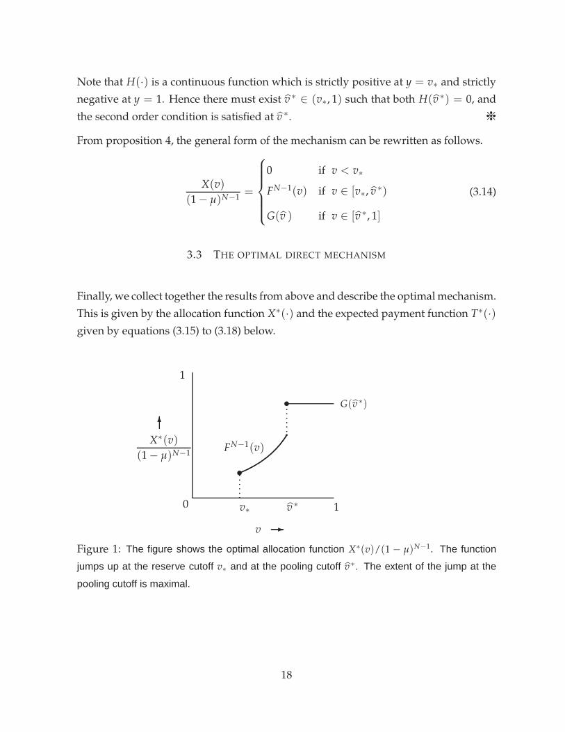
Finally, we collect together the results from above and describe the optimal mechanism.

This is given by the allocation function X∗(·) and the expected payment function T∗(·)

given by equations (3.15) to (3.18) below.

G(v ∗)

10

1

X∗(v)

(1 − µ)N−1

6

v -

FN−1(v)

v∗ v ∗

t

t

Figure 1: The figure shows the optimal allocation function X∗(v)/(1 − µ)N−1. The function

jumps up at the reserve cutoff v∗ and at the pooling cutoff v ∗. The extent of the jump at the

pooling cutoff is maximal.

18

X∗(vh) =N−1

∑n=0

(N − 1

n

)(1 − µ)N−n−1µn 1

n + 1, (3.15)

X∗(v) =

0 if v < v∗

(1 − µ)N−1 FN−1(v) if v ∈ [v∗, v ∗)

(1 − µ)N−1 G(v ∗) if v ∈ [v ∗, 1]

(3.16)

T∗(vh) = vhX∗(vh)− (vh − 1) X∗(1) −∫ 1

0X∗(t) dt, (3.17)

T∗(v) = vX∗(v) −∫ v

0X∗(t) dt for v ∈ [0, 1]. (3.18)

where the “reserve type” v∗ is given by ψ(v∗) = 0, G(·) is given by equation (3.13),

and the “pooling cutoff” v ∗ maximizes the expression in proposition 4.

X∗(vh) follows from equation (3.8), and T∗(vh) follows from equation (3.5). The op-

timal allocation X∗(v) follows from equation (3.14). T∗(v) then follows from equa-

tion (3.2). Figure 1 shows the optimal mechanism.

Also note that other than the pooling of types in [v ∗, 1] and the presence of the reserve

type v∗, the optimal mechanism is efficient. Whenever at least one bidder draws a type

above v∗, the object is sold with probability 1. We now present a simple numerical

example to elucidate the design of the optimal direct mechanism.

3.4 AN EXAMPLE

Suppose N = 2 and suppose the bidders draw values from a uniform distribution over

the unit interval. Then F(v) = v, and f (v) = 1 for all v ∈ [0, 1]. From equation (3.7),

the modified virtual value is given by

ψ(v) = 2v(1 − µ)− 1. (3.19)

The optimal mechanism is trivial if it involves a pure posted price of vh In this case

the seller simply sells to the high type and does not sell to any other lower types. For

the optimal mechanism to involve selling to lower types as well, we need to satisfy

assumption 2, which requires µ <1

2. From proposition 2, we also need λ(v∗) > 0.

19

Using the value of ψ(v) from above, this requires 4µ(1 − µ)vh < 1. Solving for µ and

using the restriction µ < 1/2, we get the following constraint on µ which must be

satisfied for a non-trivial mechanism.

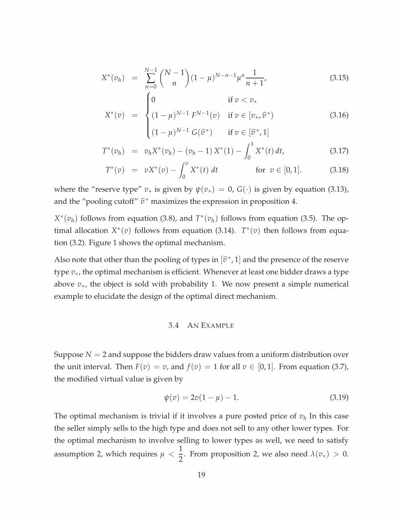
µ <1

2

(1 −

√vh − 1

vh

)≡ µ(vh) (3.20)

Figure 2 shows this upper limit.

2 3 4 5

0.1

0.2

0.3

0.4

0.5

1

µ(v )h

Pure posted price

Posted price

plus optimal auction

µ

vh

Figure 2: For any (µ, vh) to the left of µ(vh), the optimal mechanism is to have a posted

price plus an optimal auction, which itself includes a pooling region (which, as the next section

shows, implies an auction with a buy-now price). In the region to the right of µ(vh), the optimal

mechanism coincides with a pure posted price of vh.

For any µ < µ(vh), the optimal mechanism involves an auction. Under a uniform

distribution, the reserve type v∗ (given by ψ(v∗) = 0), and the “pooling cutoff” v ∗

(given by equation (??)) are

v∗ =1

2(1 − µ)

v∗ = 1 −

√µ(vh − 1)

1 − µ

From equation (3.6), the expected revenue is given by

ER = 2

[µvhX∗(vh)− µ (vh − 1) X∗(1) +

∫ 1

0ψ(v)X∗(v) f (v)dv

]

20

where X∗(·) is specified in the previous section. For µ > µ(vh), the optimal mechanism

is a posted price of vh and the expected revenue is(18)

ER = 2µvhX∗(vh)

Finally consider a mechanism that combines a posted price with a standard auction.

This is clearly suboptimal(19), but calculating the expected revenue from this mecha-

nism clarifies the gain from the pooling at the top in the optimal auction. The expected

revenue from the suboptimal mechanism is given by

ER = 2

[µvhX∗(vh)− µ (vh − 1) X(1) +

∫ 1

0ψ(v)X(v) f (v)dv

]

where X∗(vh) is as before, but now X(·) = (1 − µ)F(v) for all v ∈ [v∗, 1].

As an example, consider vh = 1.5 and µ = .1. Since µ(1.5) = 0.21, the optimal mecha-

nism involves a posted price and an auction. The auction is characterized by v∗ = .56

and v∗ = .76, i.e. the lowest 56% types are not served and the top 24% types in the

unit interval are pooled. The revenue from the optimal mechanism is 0.47. A simple

posted price fetches a revenue of .29. Thus there is a gain from price discrimination.

The following figure shows the optimal mechanism.

��

��

.88

10

1

X(v)

(1 − .1)

6

v -

v

.56 .76

s

s

Figure 3: The optimal allocation function X∗(v)/(1 − µ) for µ = .1 and vh = 1.5.

(18)Alternatively, this can be derived as vh times the probability that at least one bidder is of type vh, i.e.

ER = (1 − (1 − µ)2)vh.(19)Such an auction (with the right reserve price) is optimal in the standard independent private values

setting (i.e. without an atom at vh), but suboptimal in our setting.

21

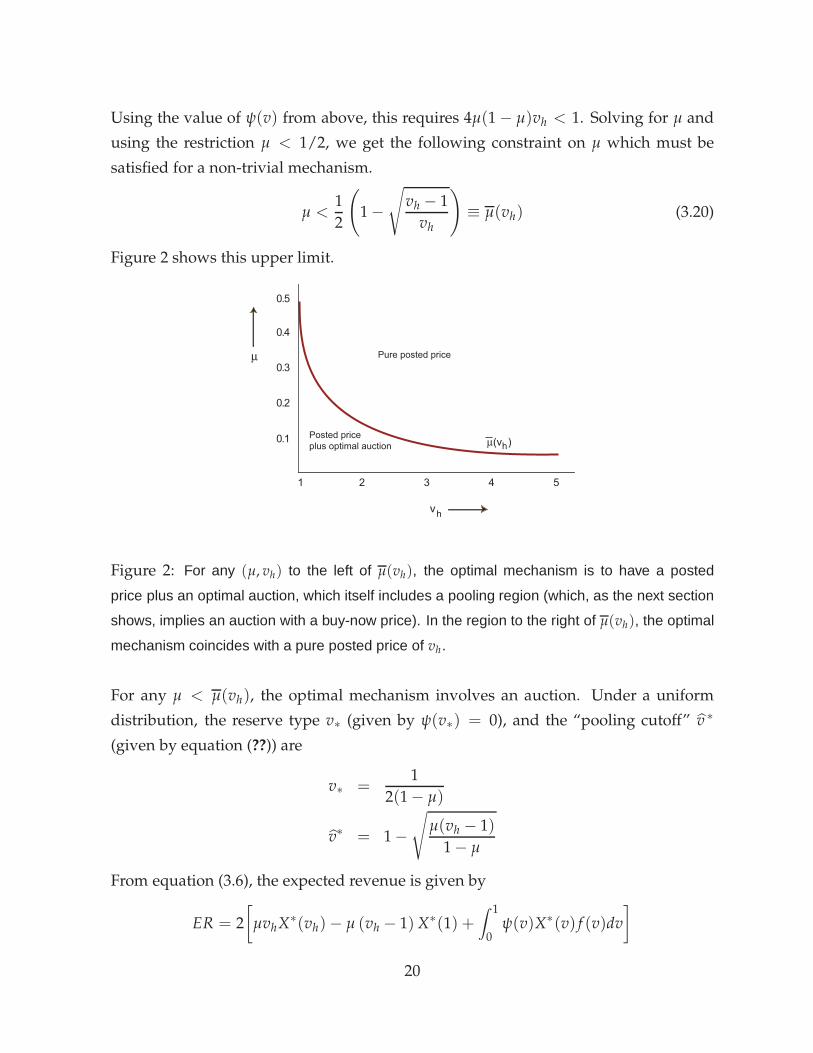
Figure 4 shows the expected revenue from the optimal mechanism for different values

of vh for µ = .1. For vh < 2.78, the optimal mechanism involves an auction, and the

dotted line shows the revenue if instead of the optimal mechanism, a pure posted price

of vh is used. The figure clarifies the revenue gain from price discrimination.

2.78 4

0.48

0.76

0.19

Posted price

plus optimal auction

Pure posted price

1

ER

vh

Figure 4: The expected revenue from the optimal mechanism for µ = .1 under different values

of vh. For vh < 2.78 the optimal mechanism involves a posted price as well as price discrimina-

tion through an auction, and generates more revenue compared to a simple posted price. For

higher values of vh the optimal mechanism coincides with a simple posted price of vh.

The following table now compares the expected revenue from the optimal mechanism

(ER Opt), posted price plus standard auction (ER Std), and a pure posted price mecha-

nism (ER PP) across different values of vh. The numbers reported are for µ = 0.1. The

table compares revenue for vh ∈ [1, 2.75]. For vh 6 2.75, µ(vh) > 0.1. Therefore over

this range of vh, the optimal mechanism involves non-trivial price discrimination, and

generates more revenue than a pure posted price mechanism. The table also shows

the gain from using the optimal mechanism compared to a mechanism that combines

a posted price with a standard auction. Finally, the table compares the values of the

optimal posted price (PP Opt) with the posted price if a standard auction is used (PP

Std). For either mechanism, the posted price is given by T(vh)/X(vh).

22

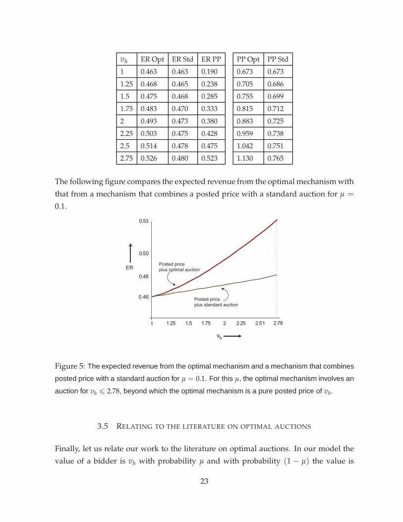
vh ER Opt ER Std ER PP PP Opt PP Std

1 0.463 0.463 0.190 0.673 0.673

1.25 0.468 0.465 0.238 0.705 0.686

1.5 0.475 0.468 0.285 0.755 0.699

1.75 0.483 0.470 0.333 0.815 0.712

2 0.493 0.473 0.380 0.883 0.725

2.25 0.503 0.475 0.428 0.959 0.738

2.5 0.514 0.478 0.475 1.042 0.751

2.75 0.526 0.480 0.523 1.130 0.765

The following figure compares the expected revenue from the optimal mechanism with

that from a mechanism that combines a posted price with a standard auction for µ =

0.1.

1.25 1.5 1.75 2 2.25 2.51 2.78

0.48

0.50

0.53

0.46

Posted price

plus optimal auction

Posted price

plus standard auction

1

ER

vh

Figure 5: The expected revenue from the optimal mechanism and a mechanism that combines

posted price with a standard auction for µ = 0.1. For this µ, the optimal mechanism involves an

auction for vh 6 2.78, beyond which the optimal mechanism is a pure posted price of vh.

3.5 RELATING TO THE LITERATURE ON OPTIMAL AUCTIONS

Finally, let us relate our work to the literature on optimal auctions. In our model the

value of a bidder is vh with probability µ and with probability (1 − µ) the value is

23

drawn from a distribution F(·) (with density f (·)) on the domain [0, 1]. Instead, con-

sider a distribution F (·) on [0, vh + ǫ] where the density is (1 − µ) f on [0, 1], ǫ on

(1, vh) and 1ǫ (µ − ǫ(vh − 1)) on [vh, vh + ǫ]. This “perturbed” distribution is within the

scope of the analysis of Myerson (1981). It is instructive to see that the pooling result

we obtain here can be obtained from the standard methods applied to this perturbed

distribution, and that the mechanism constructed here can be obtained by a limiting

argument.(20)

Since the limiting case is the one we are interested in, and since one cannot directly

apply the standard methods in this case, we have derived the optimal mechanism di-

rectly. As a minor technical point, our results can be taken as a verification that there

is no discontinuity in the optimal mechanism in the limit. The optimal mechanism for

distributions away from the limit (derived using standard methods), converge to the

one we derive for the limiting case.

To derive the optimal mechanism for the perturbed distribution, we adopt the “marginal-

revenue” approach of Bulow and Roberts (1989) who reinterpret the problem of de-

signing an optimal auction as a standard monopolist’s problem. Define q = 1 − F(v)

as quantity and v as price. The (inverse) “demand curve” is given by:

v(q) =

vh + ε −εq

µ − (vh − 1)εif 0 6 q 6 µ − (vh − 1)ε

vh −q − µ + (vh − 1)ε

εif µ − (vh − 1)ε < q < µ

F−1(

1 − q−µ1−µ

)if µ 6 q 6 1

The corresponding marginal revenue (MR) is given by

MR(q) =

MR1(q) ≡ vh + ε −εq

µ − (vh − 1)εif 0 6 q 6 µ − (vh − 1)ε

MR2(q) ≡ vh −q − µ + (vh − 1)ε

εif µ − (vh − 1)ε < q < µ

MR3(q) ≡ F−1(

1 −q−µ1−µ

)−

q

(1−µ) f(

F−1(

1−q−µ1−µ

)) if µ 6 q 6 1

MR2 and MR3 are clearly decreasing in q. By rewriting as a function of v, it is easy

to check that MR1 is simply the modified virtual value, and thus assumptions 1 and 2

ensure that this is decreasing in q and present a non-trivial optimization problem.

(20)We are grateful to a referee for pointing this out.

24

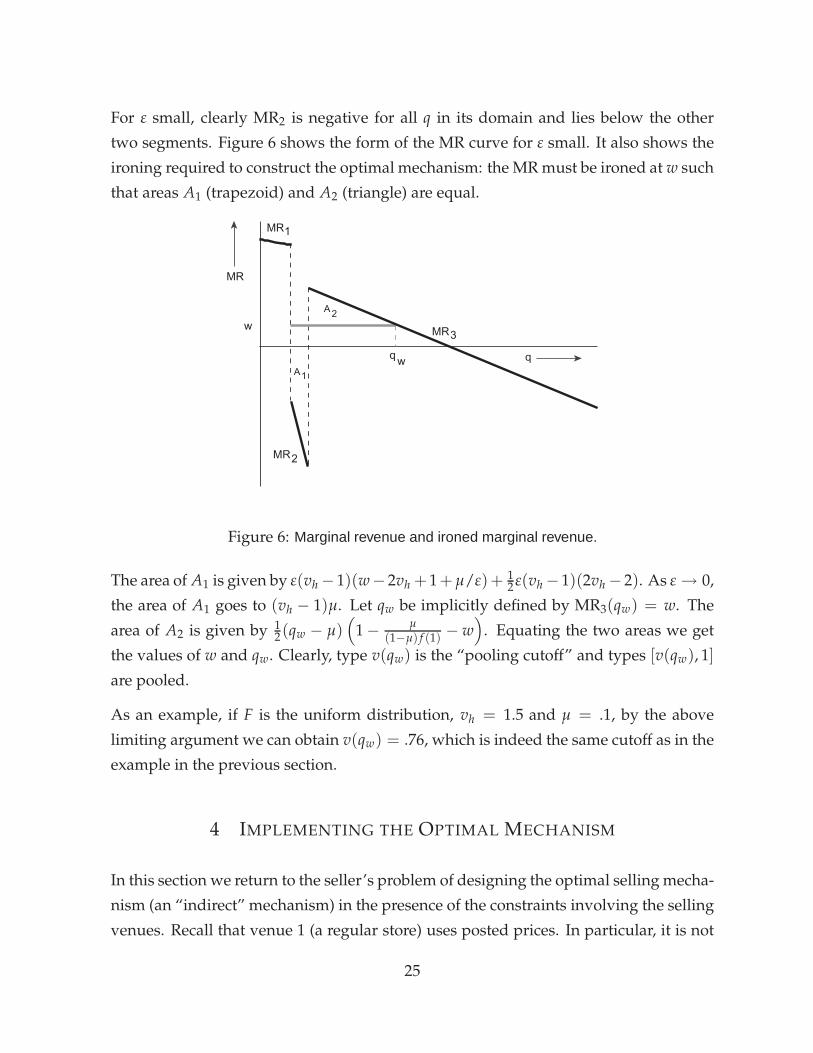
For ε small, clearly MR2 is negative for all q in its domain and lies below the other

two segments. Figure 6 shows the form of the MR curve for ε small. It also shows the

ironing required to construct the optimal mechanism: the MR must be ironed at w such

that areas A1 (trapezoid) and A2 (triangle) are equal.

q

MR1

MR2

MR3

MR

A1

A2

w

qw

Figure 6: Marginal revenue and ironed marginal revenue.

The area of A1 is given by ε(vh − 1)(w− 2vh + 1 + µ/ε)+ 12 ε(vh − 1)(2vh − 2). As ε → 0,

the area of A1 goes to (vh − 1)µ. Let qw be implicitly defined by MR3(qw) = w. The

area of A2 is given by 12(qw − µ)

(1 −

µ(1−µ) f (1)

− w)

. Equating the two areas we get

the values of w and qw. Clearly, type v(qw) is the “pooling cutoff” and types [v(qw), 1]

are pooled.

As an example, if F is the uniform distribution, vh = 1.5 and µ = .1, by the above

limiting argument we can obtain v(qw) = .76, which is indeed the same cutoff as in the

example in the previous section.

4 IMPLEMENTING THE OPTIMAL MECHANISM

In this section we return to the seller’s problem of designing the optimal selling mecha-

nism (an “indirect” mechanism) in the presence of the constraints involving the selling

venues. Recall that venue 1 (a regular store) uses posted prices. In particular, it is not

25

practical for the seller to run an auction at venue 1. Venue 2 is an (online) auction site.

The seller can access venue 1 at zero cost and venue 2 by incurring a cost of c > 0. The

seller can optimally choose the posted price at venue 1 and the auction format at venue

2.

We solve the seller’s problem by establishing that the seller can in fact implement(21)

the optimal direct mechanism from the previous section with a two stage mechanism

even under the additional venue restrictions.(22) Further, the two stage mechanism

also uses the two venues optimally. Therefore the two stage mechanism is the optimal

mechanism in our model.

The mechanism works as follows. The first stage involves a posted price P at venue 1.

If the object is not sold in the first stage then the seller uses venue 2 where the mecha-

nism used is an auction involving a buy-now option. We also show that the buy-now

option is temporary rather than permanent. We discuss this point further after describ-

ing the selling mechanism, and show that a permanent buy price cannot implement

the optimal mechanism.

4.1 DESCRIPTION OF THE SELLING MECHANISM

The selling mechanism is implemented in two stages. Stage 1 takes place at venue 1

(store using posted price). Stage 2 is carried out at venue 2 (auction site).

Stage 1. (Posted Price) The item is offered for sale at a posted price P. If any buyer

wants to buy at that price, the item is sold and the game is over. If there is a tie, it

is resolved by randomly allocating the item to one of the tied buyers. If the item

is not sold, we proceed to stage 2.

Stage 2. (Auction) This is an auction augmented by a buy-now option. Let B denote

the buy price. Stage 2 has two sub-stages.

First sub-stage. (buy-now option) In the first sub-stage, the auction opens with a buy

price B. If a single bidder bids B, the object is awarded to that bidder. If two or

(21)In the sense that the probability allocation in the indirect game are the same as those in the direct

revelation game; the seller’s expected profit is, of course, smaller (and depends on the value of c).(22)We remind the reader that the direct revelation game in the previous section addressed the same

optimization problem except that it ignored restrictions posed by the presence of heterogeneous venues.

26

more bidders submit B, the object is allocated randomly with the winning bidder

paying the price B. If no bidder bids B, the game proceeds to the second sub-

stage.

Second sub-stage. (Vickrey auction) The second sub-stage is a standard Vickrey auc-

tion with a reserve price. In this stage the object is allocated to the highest bidder

at a price which is the maximum of the reserve price and the second highest bid

provided the highest bid is above the reserve price. If the highest bid is below

the reserve price, the seller keeps the object and the game is over.

We now show that this selling mechanism implements the optimal direct mechanism

from the previous section, and is also the optimal mechanism taking into account the

venue restrictions.

4.2 IMPLEMENTATION

To economize on notation, in what follows we refer to the optimal pooling cutoff as v

(rather than v ∗).

Proposition 6. The two stage selling mechanism described above implements the optimal direct

mechanism when the reserve price in the Vickrey auction is chosen as v∗, and the posted price

P and temporary buy price B are chosen as:

P = vh −(1 − µ)N−1

X∗(vh)

[(vh − F(v )

)G(v ) +

∫ v

v∗F N−1(t) dt

](4.1)

B = v −1

G(v )

∫ v

v∗F N−1(t) dt (4.2)

where X∗(vh) = ∑N−1n=0 (N−1

n )(1 − µ)N−n−1µn 1n+1 , v∗ is given by ψ(v∗) = 0, and v is given

by proposition 4.(23) Finally, the two stage mechanism makes optimal use of the venues.

(23)Reynolds and Wooders (2008) analyze auctions with a temporary buy price. It is worth noting that

equation (4.2) coincides with the equation in their proposition 1 determining the cutoff value beyond

which buyers accept the buy price. The difference, of course, is that unlike Reynolds-Wooders, here the

reserve price and the cutoff v are not arbitrary but derived as parts of an optimal mechanism. Given

optimal values of the reserve price and the cutoff, we determine the buy price. Reynolds-Wooders, on

the other hand, start from any given reserve price and buy price and determine the cutoff.

27

Proof. STEP 1. (Comparing with the optimal direct mechanism) Consider the fol-

lowing strategies: Type vh buys the object in stage 1 by paying the posted price P.

Types in the interval [v, 1] submit the buy price B in the first sub-stage of stage 2. Types

in [v∗, v ) submit their true valuations as bids in the second sub-stage. (Types below v∗

do not win the object so it is irrelevant whether they participate or not. Without loss of

generality, assume they submit bids equal to their valuations also.)

Given the strategies, type vh is the only type to buy at price P which means that if a

buyer of type vh follows the prescribed strategy, the expected probability of winning

the object is the same as X∗(vh) (given by equation (3.15)).

Using the values of X∗(vh) and X∗(v) for v ∈ [0, 1], we get

∫ 1

0X∗(t) dt = (1 − µ)N−1

[∫ v

v∗F N−1(t) dt + (1 − F(v ))G(v )

]

Substituting in equation (3.17),

T∗(vh) = vh

(N−1

∑n=0

(N − 1

n

)(1 − µ)N−n−1µn 1

n + 1

)

− (1 − µ)N−1

[(vh − F(v )

)G(v ) +

∫ v

v∗F N−1(t) dt

]

Hence, if the posted price P is given by equation (4.1), the expected payment of type vh

is the same in the indirect mechanism as it is in the optimal mechanism. For types in

[v∗, v ), the probability of winning and expected payments are exactly as in the optimal

mechanism (given by equation (3.16)) since they are simply taking part in a Vickrey

auction. The types in [v, 1] also have the same expected probability of winning as in

the optimal mechanism since if they submit the buy price, they are being “pooled” in

the indirect mechanism in the same way as in the optimal direct mechanism. Now,

the expected payment of these pooled types in the optimal mechanism is given by

v X∗(v ) −∫ v

0X∗(t) dt. Since

∫ v

0X∗(t) dt = (1 − µ)N−1

∫ v

v∗F N−1(t) dt, the expected

payment of the pooled types can be written as

(1 − µ)N−1

[v G(v )−

∫ v

v∗F N−1(t) dt

]

Conditional on reaching stage 2, if a type v ∈ [v, 1] bids B, the expected payment is

G(v )B, and hence this type’s overall expected payment from participating in the mech-

28

anism is given by (1 − µ)N−1G(v )B. Thus if the buy price B is given by equation (4.2),

the expected payments are the same in the direct and the indirect mechanisms.

STEP 2. (Checking for equilibrium) We now show that the strategies described

above do constitute an equilibrium. From the way the payoffs are constructed, type

vh is indifferent between buying at the price P at the first stage and waiting to bid B

in the second stage and strictly prefers buying at price P to bidding any other price in

the second sub-stage auction. Consider now a type v ∈ [0, 1]. It is clear that no such

type wants to mimic type vh and buy the object in the first stage. To derive the opti-

mal bid of a type v ∈ [0, 1] in the second stage, all we need to do is to compare the

type’s expected payoff from only two possible bids: bidding the buy price B in the first

sub-stage, or bidding the true value of v in the Vickrey auction in the second sub-stage.

Let D(v) denote the difference in expected surplus of type v from the bids B and v. The

proof now proceeds through the following lemma, which is proved in the appendix.

Lemma 1. D(v) is strictly increasing in v and D(v ) = 0.

This shows that, as required, type v is indeed indifferent between bidding B and v.

Further, since D′(v) > 0, types below v strictly prefer to bid their true value rather

than B, and types v ∈ (v, 1] strictly prefer to bid B.

Since the mechanism implements the same probability allocation as derived in the last

section without the venue-restriction constraint, there cannot be a more profitable al-

location.

STEP 3. (Optimal use of venues) Finally, it is straightforward to verify that the indi-

rect selling mechanism described above makes optimal use of venues. By assumption,

the seller does not want to use a posted price mechanism only and so using only venue

1 is not a better alternative. Of course by using only venue 2 and having two sequen-

tial posted price offers followed by the standard Vickrey auction would also give rise to

the same expected allocation probabilities and expected revenues as in the mechanism

described in this section. Thus, it is possible to not use venue 1 at all but still imple-

ment the allocation and revenue from the direct mechanism. However since there is

the additional cost c of using venue 2, this would reduce overall expected profit by an

amount [1 − (1 − µ)N ]c. It is thus better for the seller to use the store (venue 1) first

and to use the auction site (venue 2) only when the object is not sold at the store. ❈

29

The two stage mechanism implements the optimal direct allocation ignoring venue

restrictions. It also makes optimal use of venues. Therefore even when we incorporate

the venue restrictions, it remains an optimal selling arrangement.

4.3 PROPERTIES OF THE SELLING MECHANISM: A TEMPORARY BUY-NOW OPTION

We now clarify that the indirect mechanism which implements the optimal direct mech-

anism includes a temporary buy-now option. Later, in section 4.5 we point out the con-

nection between the temporary buy-now option we use and the one used by eBay.

In stage 2 of the selling mechanism described in the previous (sub)section, bidders

are offered the chance to buy the item at price B, followed by a Vickrey auction. In

other words, the mechanism involves an auction but with a buy-now option that is

only temporary - the option is withdrawn when the actual auction takes place. It is

interesting to note that under such a buy-now option, the auction price can actually

exceed the buy price. To see this, note that types above v plan to buy the item at buy

price B and types [v∗, v ) follow the standard strategy of a Vickrey auction. Hence, at

the auction stage, the price range belongs to the interval [v∗, v] and since B < v (see

equation (4.2)), once the buy-now option vanishes, the subsequent auction price in the

optimal mechanism could be higher than the buy price.

4.4 SUBOPTIMALITY OF A PERMANENT BUY-NOW OPTION

As noted in the introduction, the literature has focused mainly on augmenting stan-

dard auctions with a permanent buy price feature and has remarked that this generates

more revenue compared to a standard auction augmented by a temporary buy-price

auction. We show, on the other hand, that in general it is not possible to implement

our optimal mechanism with a permanent buy price.

Papers by Reynolds and Wooders (2008) and Hidvegi, Wang, and Whinston (2006) (hence-

forth HWW) analyze an English auction augmented by a permanent buy price b.(24) We

(24)It should be noted that their basic environment is different from ours. They have a standard private-

value auction setting, and the distribution of values does not have a counterpart of the atom at vh that

30

make use of some of their results to show that in our context a permanent buy price is

suboptimal.(25)

Result (HWW): Consider an independent private values setting with bidders drawing

values from a distribution on [v, v]. Consider an English auction with a reserve price

r and permanent buy price b. In (the unique) equilibrium, there are cutoffs vc and

vuc such that the type space can be partitioned into the following (possibly empty)

intervals:

• types v ∈ [r, b) use a “traditional strategy” : remain active till price rises to v,

• types v ∈ [b, vc) use a “threshold strategy” : remain active till the auction price

reaches a critical point t(v, b) and then jumps to the buy price b.

• types v ∈ [vc, vuc) use a “conditional strategy” : bid b if (and only if) the auctions

clocks moves from r (implying that there is at least one other bidder with value

above r), and

• types v ∈ [vuc, v] use an “unconditional strategy” : bid b right at the start of the

auction.

The threshold t(v, b) is decreasing in v, and if limv→v t(v, b) ≥ r, vc = vuc = v, and all

types v > b play the threshold strategy. On the other hand if limv→v t(v, b) < r, there

are types who play the conditional and unconditional strategies.

Translating this to our context, given a permanent buy price B and the reserve type

v∗, a posted price followed by an auction can implement the optimal mechanism if

types [v, 1] play the unconditional strategy (i.e. bid B immediately) and types [v∗, v )

play strategies such that their bids are revenue-equivalent to the bids in the temporary

buy-price auction.

It is clear that in the temporary buy-price auction (as in the optimal direct mechanism),

only types v ∈ [v, 1] are pooled, and there is no pooling in the interval [v∗, v ). In this

interval the allocation probability and expected payment are strictly increasing. There-

fore if any indirect mechanism involves pooling (same allocation probability, same ex-

features in our model. However, this distinction is not important for what follows.(25)Reynolds and Wooders (2008) describe threshold strategies (a bidder bids as in an usual English

auction up to a threshold, then accepts the buy price), and add an assumption of “no-regret” to ensure

existence. HWW use a strategy specification that ensures existence under general conditions. In what

follows we use the treatment of HWW.

31

pected payment) in the latter region, this would introduce additional inefficiency, and

prevent the mechanism from implementing the optimal mechanism.

Consider an auction with a permanent buy price B. Types playing the conditional strat-

egy or unconditional strategy are clearly pooled. Therefore to avoid pooling of types

below v, it must be that no sub-interval of types in [v∗, v ) play either the conditional or

unconditional strategies. But from the result above, we know that this happens if and

only if limv→v t(v, B) ≥ v∗. We state this below.

Corollary: A necessary condition for implementing the optimal direct mechanism us-

ing a posted price combined with an English auction with a permanent buy price B is

given by limv→v

t(v, B) > v∗.

Can we ensure this condition holds? As the following result shows, the problem is that

v, B as well as the function t(·, ·) are already determined by conditions of implemen-

tation of the optimal mechanism. Thus there is no parameter we could vary to ensure

this inequality holds. It might hold for some distribution F by lucky coincidence, but

in general it is not possible to ensure this. The proof of the following result shows that

the inequality is not satisfied for a uniform distribution.

For the following result, we use the usual definition of implementation: for any dis-

tribution F (satisfying the basic assumptions) an indirect mechanism implements the

optimal mechanism if there exists an equilibrium of the indirect mechanism whose

outcome is the same as that of the optimal mechanism. The following result shows

that a permanent buy-now option fails this test.

Proposition 7. It is not possible to implement the optimal direct mechanism using an English

auction with a permanent buy price B.

Proof. Since the indirect mechanism, by definition, is required to implement the op-

timal mechanism for all allowable parameter values and distributions, it suffices to

provide an example where it does not. In particular, we show here that for N = 2,

under a uniform distribution, limt→v t(v, B) < v∗, so that the necessary condition for

implementation identified in the corollary above is violated.

We have already shown that an auction with a temporary buy price does implement

the optimal mechanism. If an auction with a permanent buy price also implements the

32

optimal mechanism, all types should win with the same probability and get the same

expected surplus in the two buy-price auctions.

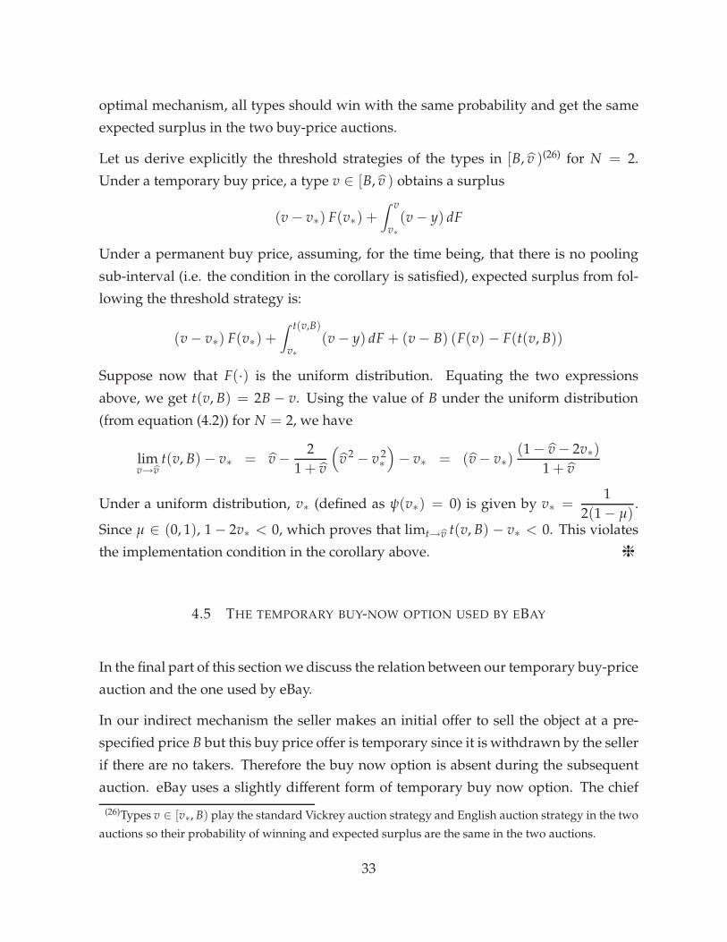
Let us derive explicitly the threshold strategies of the types in [B, v )(26) for N = 2.

Under a temporary buy price, a type v ∈ [B, v ) obtains a surplus

(v − v∗) F(v∗) +∫ v

v∗(v − y) dF

Under a permanent buy price, assuming, for the time being, that there is no pooling

sub-interval (i.e. the condition in the corollary is satisfied), expected surplus from fol-

lowing the threshold strategy is:

(v − v∗) F(v∗) +∫ t(v,B)

v∗(v − y) dF + (v − B) (F(v) − F(t(v, B))

Suppose now that F(·) is the uniform distribution. Equating the two expressions

above, we get t(v, B) = 2B − v. Using the value of B under the uniform distribution

(from equation (4.2)) for N = 2, we have

limv→v

t(v, B) − v∗ = v −2

1 + v

(v 2 − v 2

∗

)− v∗ = (v − v∗)

(1 − v − 2v∗)

1 + v

Under a uniform distribution, v∗ (defined as ψ(v∗) = 0) is given by v∗ =1

2(1 − µ).

Since µ ∈ (0, 1), 1 − 2v∗ < 0, which proves that limt→v t(v, B) − v∗ < 0. This violates

the implementation condition in the corollary above. ❈

4.5 THE TEMPORARY BUY-NOW OPTION USED BY EBAY

In the final part of this section we discuss the relation between our temporary buy-price

auction and the one used by eBay.

In our indirect mechanism the seller makes an initial offer to sell the object at a pre-

specified price B but this buy price offer is temporary since it is withdrawn by the seller

if there are no takers. Therefore the buy now option is absent during the subsequent

auction. eBay uses a slightly different form of temporary buy now option. The chief

(26)Types v ∈ [v∗, B) play the standard Vickrey auction strategy and English auction strategy in the two

auctions so their probability of winning and expected surplus are the same in the two auctions.

33

distinction is that in the eBay auction the disappearance of the buy price is endogenous:

the buy-now option vanishes whenever a bidder places a bid above the reserve price.

Even though the eBay auction differs from ours, we now argue that in the scenario

modeled here, the outcome of the two should be the same. To see this, recall the four

possible strategies in a buy-price auction from the HWW result stated in section 4.4

above. These are traditional, threshold, conditional and unconditional strategies. Now,

the threshold strategy (under which a bidder waits for the price in the auction to rise

to a certain level before exercising the buy-now option), and the conditional strategy

(under which a bidder waits and bids the buy price only if some other bidder bids

above the reserve price) are not available under the rules of eBay auctions, since in

both cases the buy-now option would vanish. Therefore, in an eBay buy-price auction,

only two – the standard and the unconditional strategies – are feasible. But this is just

like our selling mechanism. Hence, under the setting of our model, the optimal eBay

auction is to choose the reserve price and the buy price to be v∗ and B respectively, and

in this case the eBay auction should implement the optimal mechanism.

5 CONCLUSION

We study the optimal price discriminating mechanism across heterogeneous venues,

and relate our results to a widely used but seemingly suboptimal online auction for-

mat. The starting point of our analysis is the observation that in addition to traditional

posted price selling through bricks-and-mortar stores (as well as own web sites), sell-

ers can now access online auction sites as a sales channel. Such auctions often enable

sellers to reach buyers who are typically priced out in traditional markets. Since the

sellers use different sales mechanisms to target different groups of buyers, the optimal

design of the overall mechanism involves second degree price discrimination across

selling methods.

We assume that the seller has access to a sales venue such as a store that can only use

a posted price, and can also pay a small fee to access an (online) auction site, which

allows unrestricted design of the sales mechanism. We characterize the optimal sell-

ing mechanism in this environment, and show that it involves a posted price at the

store and an auction where there is “pooling at the top” amongst the types who decide

34

to participate in the auction. This feature of the optimal mechanism corresponds ex-

actly to a buy-now option. Thus, the phenomenon of a buy-now option in an auction,

something that might appear puzzling when seen in isolation (i.e. in the context of the

auction alone) emerges as a necessary feature of the overall optimal selling mechanism.

Interestingly, we show that posted price selling followed by a standard auction with

a temporary buy-now option – used by eBay and seemingly even more of a puzzling

phenomenon(27) – implements the optimal mechanism, but the same is not true of an

auction with a permanent buy-now option.

Of course, eBay as well as other online auctions are rich in institutional detail. While

we do not claim to capture all of these, we do believe that for many sellers online

auctions form part of an optimal selling strategy across heterogeneous venues, and

therefore it is important to understand the overall strategy in order to analyze its con-

stituent parts. While other theories have sought to explain a buy-now option as an

improvement over a standard auction in certain cases (e.g. risk averse bidders), this is

the first paper to explain such an option as part of an optimal mechanism. However,

further empirical tests taking into account overall market data are required to distin-

guish between competing theories. To this end, we briefly mention how the testable

implications of our model differ from other theories.

TESTABLE IMPLICATIONS

The risk-aversion-based theory as well as other approaches mentioned in the introduc-

tion look at auctions in isolation. An implication is that there is no systematic relation

between prices posted elsewhere by the seller for similar goods and the buy price in

the auction. A further implication of the risk aversion theory is that if similar items

are offered for sale through posted prices elsewhere, this might weaken the incentive

to have a buy price, since the most risk averse buyers might prefer to buy at a posted

price. Thus the theory implies that if similar items are sold elsewhere through posted

prices by a seller, this makes it less likely that the seller would use a buy-now option.

The theory presented here, on the other hand, shows that posted price sales make it

(27)Indeed, as noted in the introduction, the literature often concludes that auctions with a temporary

buy-now option are revenue inferior to those with a buy-now option that is permanent.

35

more likely that the seller uses a buy price in the auction. Further, our theory predicts

a negative relation between the posted price and the buy price. A higher posted price

necessitates greater inefficiency in the auction to preserve incentives. Further empirical

work is needed to test the relative importance of theories in explaining the emergence

of a buy-now option in standard auctions.

36

6 APPENDIX: PROOFS

A.1 PROOF OF PROPOSITION 4

From (3.11), the objective is to maximize

∫ v

v∗ψ(v)X(v) f (v) dv +

[−µ(vh − 1) +

∫ 1

vψ(v) f (v) dv

]X(v )

We know from equation (3.12) that all terms in the expression for X(v) contain a com-

mon factor (1 − µ)N−1. Define Y(v) ≡X(v)

(1 − µ)N−1. Without loss of generality, we can

optimize in terms of Y(v) rather than X(v).

Equation (3.12) specifies Y(v). Let us find the optimal βn(·) for any given value of

n ∈ {1, . . . , N − 1}. Let Y(v, n) denote the relevant term for this n in the summed

expression Y(v).

Let ρ(n) ≡ (N−1n ) (1 − F(v ))N−1−n.

Suppose βn(·) is not always zero, and let

Y(v, n) = (1 − θ)G(v ) for v ∈ [v, 1] (A.1)

where θ ∈ (0, 1) and fixed exogenously. From the expression for Y(v), this implies we

must obey the constraint

ρ(n)

N − n

∫ v

v∗βn(t) dF n = θG(v ) (A.2)

Further, incentive compatibility requires

Y(v−) ≡ limv↑v

Y(v) 6 (1 − θ)G(v ) (A.3)

For any given (v, θ), the optimization problem can be written (using equations (3.12)

and (A.1)) as

maxβn(v)

∫ v

v∗ρ(n − 1)βn(v)F n−1(v)ψ(v) f (v) dv +

∫ v

v∗F N−1(v)ψ(v) f (v) dv

+

[−µ(vh − 1) +

∫ 1

vψ(v) f (v) dv

](1 − θ)G(v )

37

subject to (A.2) and (A.3).

Given (v, θ), the second and third terms are constant terms. Thus the optimization

problem is simply given by the first term, which can be rewritten so that the maxi-

mization problem is:

maxβn(v)

ρ(n − 1)

n

∫ v

v∗βn(v)ψ(v) dF n

subject to (A.3) and (A.2).

Sinceρ(n−1)

n is a constant term, we can ignore this, and simply maximize∫ v

v∗βn(v)ψ(v) dF n.

Let us approximate the βn(v) function by a step function with s steps at v0 < v1 <

. . . < vs. Let v0 = v∗ and vs = v. Let the value of the function be β(k)n over the k-th step.

Let R denote the maximand. The optimization problem is

maxβ

(1)n ,...,β

(s)n

R

where

R ≡∫ v1

v∗β(1)

n F(v)ψ(v) dF n +∫ v2

v1

β(2)n F(v)ψ(v) dF n + . . . +

∫ v

vs−1

β(s)n F(v)ψ(v) dF n

Subject to (A.3) and (A.2), which becomes

θG(v ) =ρ(n)

N − n

[β(1)

n (F n(v1)− F n(v∗)) + . . . + β(s)n (F n(v )− F n(vs−1))

](A.4)

Let us increase β(k)n and reduce β(j)

n in a way such that the constraint is preserved. From

the constraint,

∂β(j)n

∂β(k)n

= −

(F n(vk)− F n(vk−1)

F n(vj)− F n(vj−1)

)

Using this,dR

dβ(k)n

= (F n(vk)− F n(vk−1)) Z, where

Z =∫ vk

vk−1

ψ(v)dF n

(F n(vk)− F n(vk−1))−∫ vj

vj−1

ψ(v)dF n

(F n(vj)− F n(vj−1))

Clearly, Z T 0 as k T j.

38

Therefore, if constraint (A.3) is slack to start with, it is optimal to increase β(s)n until it

binds, so that over the interval [vs−1, v ), Y(v) is raised to (1 − θ)G(v ). Therefore the

optimal β(s)n , denoted by β(s)∗

n , is given by

ρ(n)β(s)∗n F n(v ) + F N−1(v ) = (1 − θ)G(v )

At this point the incentive compatibility constraint (A.3) binds, so that β(s)n cannot be

increased any further.

Next, in the same way, increase β(s−1)n so that ρ(n)β(s−1)∗

n F n(vs−1) + F N−1(vs−1) =

(1 − θ)G(v ).

Continuing in this manner, we get ℓ ∈ 1, . . . , s − 1 such that

Φ(vℓ) > 0 and Φ(vℓ−1) < 0,

where

Φ(vℓ) =ρ(n)

N − n

s

∑k=ℓ+1

∫ vk

vk−1

β(k)∗n dF n − θ G(v )

Note that the expression on the right hand side simply reflects the constraint (A.4),

with β(k)n replaced by its optimal value for k ∈ {ℓ, . . . , s}. As we consider a finer and

finer grid (i.e. as (vk − vk−1) → 0 for all k), in the limit vℓ is such that

ρ(n)

N − n

∫ v

vℓ

β∗n(v) dF n = θ G(v )

Therefore vℓ is such that types below receive no transfer (and therefore any type v < vℓ

wins with probability F N−1(v) only), and types above vℓ are pooled.

If originally we had put βn(·) = 0 always, types above v would be pooled with ex-

pected probability of winning G(v ).

Now, types above vℓ are pooled, and types below receive no transfer. Thus, apart from

v changing to vℓ, the situation is exactly the same as the case in which βn(·) = 0.

Therefore vℓ must be such that G(vℓ) = θG(v ). Note that the solution for vℓ does

not depend on n. Therefore we can rewrite the optimization problem as the following

unconstrained maximization problem:

maxvℓ

∫ vℓ

v∗F(v)ψ(v) f (v) dv + G(vℓ)

[−µ(vh − 1) +

∫ 1

vℓ

ψ(v) f (v) dv

]

Thus the general form of the maximization problem is as stated. This completes the

proof. ❈

39

A.2 PROOF OF LEMMA 1

Case 1: v 6 v.

In stage 2, in equilibrium, the expected payment from bidding v is v∗F N−1(v∗) +∫ vv∗

t dF N−1. The second term can be rewritten as vF N−1(v)− v∗F N−1(v∗)−∫ v

v∗F N−1(t)dt.

Therefore the expected payment from bidding v can be written as

vF N−1(v) −∫ v

v∗F N−1(t)dt

The expected value is vF N−1(v). Therefore the expected net payoff from bidding v is∫ vv∗

F N−1(t)dt. The expected payoff from bidding B is (v − B)G(v ).

D(v) denotes the difference between the expected payoff from bidding B in the first

stage or v in the second stage. From the above, this is given by D(v) = (v − B) G(v )−∫ vv∗

F N−1(t)dt. Using the value of B from equation (4.2), this can be rewritten as

D(v) = (v − v )G(v ) +∫ v

vF N−1(t)dt

Clearly, D(v ) = 0. Next, D′(v) = G(v )− F N−1(v).

From equation (3.13),

G(v ) = F N−1(v ) +N−2

∑n=0

(N − 1

n

)(1 − F(v ))N−1−n F n(v )

N − n> F N−1(v ) (A.5)

Since v 6 v, G(v ) > F N−1(v). Thus D′(v) > 0.

Case 2: v > v.

The expected payment from bidding v is v∗F N−1(v∗) +∫ v

v∗t dF N−1. This simplifies

to vF N−1(v ) −∫ v

v∗F N−1(t)dt. The expected value is vF N−1(v ). Therefore the ex-

pected net payoff is (v − v) F N−1(v ) +∫ v

v∗F N−1(t)dt. Hence for types v > v, D(v) =

(v − B) G(v ) −((v − v) F N−1(v ) +

∫ vv∗

F N−1(t)dt)

. Using the value of B from equa-

tion (4.2), this can be rewritten as D(v) = (v − v )(G(v )− F N−1(v )

). Clearly, D(v ) =

0, and D′(v) = G(v )− F N−1(v ) > 0, where the last inequality follows from (A.5). ❈

40

REFERENCES

BUDISH, E. B., AND L. N. TAKEYAMA (2001): “Buy Prices in Online Auctions: Irra-

tionality on the Internet?,” Economics Letters, 72, 325–333.

BULOW, J., AND J. ROBERTS (1989): “The Simple Economics of Optimal Auctions,”

Journal of Political Economy, 97, 1060–90.

DELTAS, G. (2002): “Determining damages from the operation of bidding rings: An

analysis of the post-auction knockout sale,” Economic Theory, 19, 243–269.

HIDVEGI, Z., W. WANG, AND A. B. WHINSTON (2006): “Buy Price English Auction,”

Journal of Economic Theory, 129(1), 31–52.

HOLT, C. A. (1980): “Competitive Bidding for Contracts under Alternative Auction

Procedures,” Journal of Political Economy, 88(3), 433–445.

LUCKING-REILEY, D. (2000): “Auctions on the Internet: What’s being auctioned, and

how?,” Journal of Industrial Economics, 48(3), 227–252.

MASKIN, E. S., AND J. G. RILEY (1984): “Optimal Auctions with Risk Averse Buyers,”

Econometrica, 52, 1473–1518.

MATHEWS, T., AND B. KATZMAN (2006): “The role of varying risk attitudes in an auc-

tion with a buyout option,” Economic Theory, 27(3), 597–613.

MATTHEWS, S. (1983): “Selling to Risk Averse Buyers with Unobservable Tastes,” Jour-

nal of Economic Theory, 30, 370–400.

MILGROM, P. (2004): Putting auction theory to work, chapter 6.2.2.3. Cambridge Univer-

sity Press.

MILGROM, P., AND I. SEGAL (2002): “Envelope Theorems for Arbitrary Choice Sets,”

Econometrica, 70(2), 583–601.

MILLER, M. (2005): Making a Living from Your eBay Business. Que,

www.quepublishing.com.

MYERSON, R. (1981): “Optimal Auctions,” Mathematics of Operations Research, 6, 58–63.

REYNOLDS, S. S., AND J. WOODERS (2008): “Auctions with a Buy Price,” Economic

Theory, This issue.

41