OPTIMAL POLYPHASE SORTING bY Derek A. Zave STAN-(X-76 ...
80
OPTIMAL POLYPHASE SORTING bY Derek A. Zave STAN-(X-76-543 MARCH 1976 COMPUTER SCIENCE DEPARTMENT School of Humanities and Sciences STANFORD UNIVERSITY
Transcript of OPTIMAL POLYPHASE SORTING bY Derek A. Zave STAN-(X-76 ...

OPTIMAL POLYPHASE SORTING
bY
Derek A. Zave
STAN-(X-76-543MARCH 1976
COMPUTER SCIENCE DEPARTMENTSchool of Humanities and Sciences
STANFORD UNIVERSITY


c
Optimal Polyphase Sorting
by Derek A. Zave
Computer Science DepartmentStanford University
Stanford, California 94305
Abstract
A read-forward polyphase merge algorithm is described which performs
the polyphase merge starting from an arbitrary string distribution. This
algorithm minimizes the volume of information moved. Since this volume
is easily computed, it is possible to construct dispersion algorithms
which anticipate the merge algorithm. Two such dispersion techniques
are described. The first algorithm requires that the number of strings
to be dispersed be known in advance; this algorithm is optimal. The
second algorithm makes no such requirement, but is not always optimal.
In addition, performance estimates are derived and both algorithms are
shown to be asymptotically optimal.
Keywords and Phrases: Sorting, tape sorting, merge sorting, polyphase
sorting, tape merging, optimal merging, optimal polyphase
dispersion, blind dispersion, polyphase dispersion, Fibonacci
numbers , generalized Fibonacci numbers, Zeckendorf Theorem,
generalized Zeckendorf Theorem.
CR Categories: 5.31, 5.30.
This research was supported in part by National Science Foundation grantMCS 72-03752 AO3, -by the Office of Naval Research contract NR 044-402,and by IBM Corporation. Reproduction in whole or in part is permittedfor any purpose of the United States Government.
1

1. Introduction.-
This paper presents a mathematical analysis of the structure of the
polyphase sort with special emphasis on those properties which are related
to the performance of the sort. This analysis will enable us to construct
a poly-phase sorting algorithm with optimal performance characteristics.
We will also construct a near-optimal polyphase sort which is more suitable
for applications. Finally, we will investigate the asymptotic performance
of both of these algorithms.
Although the polyphase sort has been in use for over a decade,
comparatively little work has been done in the direction of optimizing
its performance. In an early unpublished paper [7], Sackman and Singer
developed methods for predicting the performance of the polyphase merge
and showed empirically that in certain cases that the performance of the
usual method of implementing the polyphase sort could be greatly improved.
Independently, Shell [8] developed similar techniques and used them along
with some empirical observations to construct an optimal polyphase
sorting algorithm. D. E. Knuth [5] has also investigated the optimal
polyphase sort and several of his results have been incorporated into
this paper.
k

2. The Polyphase Merge.
We will begin with a brief discussion of the polyphase merge which
will serve primarily to introduce our terminology. Further details, as
well as information on internal sorting and string merging, which we will
not discuss, may be found in the books of Flores [2] and Knuth [5].
Let us suppose that we are given a collection of records containing
various kinds of information and let us further suppose that some linear
ordering has been defined on this collection. To sort the records is to
arrange them into a sequence which is increasing with respect to the
ordering relation. One method of accomplishing this is by means of merging.
First, the collection of records is partitioned into a number of small
groups of records which each sorted to form a "string" of records.S e c o n d ,
the sorted strings are merged to form larger sorted strings, and so on,
until a single sorted string containing all of the records is formed.
In practice, merge sorts are employed when there are more records
to be sorted than may be accommodated by a computer% main storage. Groups
of records are sorted into strings using the available main storage. The
strings are then "dispersed" to some secondary storage medium such as mass
storage or magnetic tape. The string merging operations are performed as
transfers of information from one part of secondary storage to another.
The poly-phase sort is a merge sort which is characterized by the
manner in which the dispersed strings are merged. Let us suppose that
there are T > 3 tape units which are numbered from zero to t = T-l .
We define the distribution numbers Sy for i = I,...+ and n > 1 by
3

S1i=l for l<i<t- -
(24n-l
ST = St for n >l, and
s; = sy-; + St-l for n>l and 2<i<t .- -
From this definition it is easily show that for n > 1 , we have
(2*2) s"1 < s; ,< . . . -<St� l
Suppose that for some n 2 1 that Sy + . . . + St strings have been
*dispersed to the tapes in the following fashion:
tape: 0 1 2 . . . t
strings: 0 sTs; . . . St� l
We will call this configuration the perfect stage n distribution
SUITl
(2.3) Sn = s; + . . . + St"
will be called the stage n perfect number.
and the
Exampie 2.1. The following table provides some values of the distribution
numbers and perfect numbers when T = 5 (t = 4) :
n
56
78
910
nsl
1 1
1 2
2 34 6
8 12
15 23
29 44
56 85108 164
208 316
ns2
1
2
4
714
27
52100
193
372
1
2
4
8
15
29
56108
208
401
Sn
4
7
13
25
49
94181
349
673
1297
4

Suppose that we start with the perfect stage n distribution'. If
we merge together one string from each of the tapes l,...,t , then we
will obtain a single string which may be written to unit zero. If n=l,
then this operation will merge all of the strings since each tape contains
exactly one string. If n>l, then, in view of (2.2), we may perform
this operation S;f times after which we will arrive at the distribution.
tape: 0 1 2 . . . t
strings:n
sl O SE-s"l .*a SF -s"l
From the formulas (2.1) we see that this distribution is the same as
tape: 0 1 2 . . . t
strings:n-l
St 0n-ls1
n-l. . . st-l
so that if we renumber the tapes t,o,1,2,...,t-1 , then we obtain the
perfect stage n-l distribution.
By repeating this process, we obtain the perfect distributions for
stages n-2, n-3 , and so on, until we arrive at the perfect distribution
for stage one. A single merge will then produce the final sorted string.
This method of merging a perfect number of strings is called the plyphase
merge.
In practice, the distribution routine rarely produces a perfect
number of strings. In order to use the polyphase merge in this case it is
necessary to include a number of "dummy" (empty) strings in order to fill
out the-total number of strings to a perfect number. There are therefore
two choices which have to-be made before using the polyphase merge to sort
X strings. First we must choose a starting stage number n ; any n for
which x < Sn is eligible. Second, we must decide how the Sn-x dummy
5
strings are to be distributed among the x strings.
methods have been proposed for distributing the dummy
authors recommend starting with the smallest possible
we will refer to these approaches collectively as the
polmhase sort.
Although many
strings, most
stage number
standard
n ;
Since the speed of a merge is usually limited by the transfer rate
of the tape units and the speed of the merge algorithm, we see that the
time required to perform the polyphase merge is approximately proportional
to the total volume of information that moves through the merge. In
order to make this idea precise, we assume that the dispersion routine
produces strings of approximately the same size; this size will be our
unit of information, the unit string. The size of a string formed by
merging several strings is the sum of the sizes of the input strings and
the size of a dummy string is zero. We say that a string is moved when
that string or any string formed from it by a sequence of one or more
merges becomes one of the inputs for a merge. The volume of information
moved by the polyphase merge is then equal to the sum of the products of
the size of each string of the starting distribution and the number of times
that string is moved. In this paper we will show how this volume may be
minimized.
6

3. The Movement Numbers.
In general, the polyphase merge does not move all of the Sn strings
of the stage n perfect distribution the same number of times. It is
for this reason that the polyphase sort is much more difficult to analyze
than other merge sorting algorithms. However, much useful information is
supplied by the set of movement numbers M?(j) which are defined for
n>l, l_<i_<t, and all integers j by the relations
M:(l) =l for l<i_<t,
' M:(j) = 0 for j f 1 and 1 < i <t ,- -
.q(J) = $-l(j-1) for n >l, and
(3.1)
.M?J)i = M?:;(j) + My-'(j-1) for n > 1 and 2 < i <t .
We claim that M?(j) is precisely the number of strings on tape unit i
of-the stage n perfect distribution which will be moved exactly j
times by the poly-phase merge. For this to make any sense it is necessary
that M&j) be nonzero only if 1 5 j 5 n and that SF = $(l)+ . ..+~n(n) .
We wiLL prove these assertions together by induction on n . When
n=l, everything is obvious since each of the tapes l,...,t of the
perfect distribution contains exactly one string which will be moved by
the poly-phase merge exactly once. Now suppose that n >l and that
everything has been proved for stage n-l . For q(j) to be nonzero we
must have, by (3.1),%-'(j-l) + 0 or i 2 2 and g::(j) # 0 . These
inequalities imply that 15 j-l 5 n-l or 1 ,< j 5 n-l which both imply
that 1 < j-< n .- - We may show that ST = q(l)+ . ..+Mn(n) by summing
the last two formulas of (3.1) over j and by applying the corresponding
equality for stage n-l and the last two formulas of (2.1). We recall that
7

the stage n polyphase merge is performed by merging Sy strings from
each of the tapes and then by applying the stage n-l polyphase merge.
A string on unit one which will be moved j times will become part of a
string on the output tape which will be moved j-l times. Since every
string on the output tape contains exactly one string from unit one and
since the output tape becomes unit t for the stage n-l merge, we see
that unit one must contain exactly $-'(j-1) strings that will be moved
exactly j times. If 2 5 i 5-t , then a j movement string on unit i
.will either be moved to the output tape or will remain on the tape. From
similar considerations, we see that unit i must contain exactly
$%-1) + <~~(j, strings which will be moved exactly j times. This
completes the proof.
Example 3.1. Table 3.1 lists some of the movement numbers in the case
t=4.
In this paper we will make use of quite a few sets of numbers which
are defined using the movement numbers e >i j . We list the definitions:
S!$j) = $0) + . . l + q(j) ,
(34 Sn(j> = Mn(l> + . . . + Mn(j) = SF(j) + . . . + St(j) ,
G!&j) = S?(l) + . . . +'S?(j) ,
G%) = Sri(l) + . . . + Sri(j) = G:(j) + . . . + G:(j) .
In addition, we have already defined
S; = S;(n)
Sn = Sri(n) = Sf: + . . . + St .
8

In a number of the form A:(j) the superscript n is the associated
stage number, the subscript i is the number of a tape unit, and j is
some number of movements. An(j) is formed from A!?(j) by summing over
i =l,...,t and A; is formed from A;(j) by setting j = n . In a
similar fashion we may form An from A: or A"(j) .
Except for the numbers G;(j) and C?(j) , which are used in ,
connection with the volume function, the various sets of numbers which
we have defined express some simple properties of the perfect stage n
distribution:
<( 1. 3 The number of strings on unit i which will be moved
exactly j times.
M”(j) The number of strings which will be moved exactly j times.
$(j) The number of strings on unit i which will be moved at
most j times.
S”(j) The number of strings which will be moved at most j times.
S; The number of strings on unit i .
sn - The total number of strings.
A set of numbers An(j) is said to be a t-array if the following
relation is satisfied for all integers n and j:
(3.3)’ An(j) = A"-l(j-1) + . . . + AnNt(j-l) .
We will call a sum of this form a t-sum. When a t-array is represented
as a table of numbers, then we will let j index the rows and n index
the columns. It is clear that the't-array An(j) is completely determined
by its values on the vertical strip l-t < n 5 0_ (or any other strip of
width t ). We will call this strip the initialization region.
9

Most of the sets of numbers which we have defined can be expressed
as t-arrays. The t-array approach exposes many of the interesting properties
of these numbers which are obscured by the original definitions. Since all
of these numbers are defined in terms of the movement numbers, we will
begin by showing that the movement numbers may be defined as t-arrays.
For each i = l,... ,t we define the t-array A:(j) by specifying
that Aiot(0) = 1 is the only nonzero element of the initialization
region forA!☺$ l We will show that for all n 11 , l< i <t and- - -
G all j that A:(j) = M?(j) . It is clear that the only nonzero values
in the columns n = -t are Ait = 1 and Ait = -1 for 1 < i <t .-
If we let 8: denote the Kronecker Delta, then for -t < n < 0 we have- -.
' A:(j) = $:6; + 6!& and A;(j) = ~?JJ~ n j for l_< i <t .- K$o
Therefore, for l-t ,< n ,< 0 , we have
andfor 2<i<t- -
These relations correspond to the last two formulas of (3 .l) and since they
hold for n and j in the initialization region, they can be extended to
all values of n and j by a simple induction argument using the
-recurrence relation (3.3). Since the only nonzero values in the columns
n = 1 are A:(l) = 1 , we see that the numbers An&j) also satisfy the
first two relations of (3.1). We therefore conclude that q(j) = A:(j)
for all n >l .
10

Below we list the various t-arrays in which we will be interested
and specify the nonzero values in their respective initialization regions:
.qw. M;-t(0) = 1 ,
MY0 l?(o) = 1 for l-t 5 n ,< 0 ,
Siet(j) = 1 for j ,>O ,
S”(j) S"(j) = 1 for l-t L n 5 0 and j 2 0 ,
G!&j) Gimt( j) = j+l for j _>O )
Gn(j> Gn(j) = j+l for l-t ,< n ,<O and j 20 .
It is not difficult to show that these t-arrays satisfy the definitions
given in (3.2).
Example 3.2. Table 3.2 shows a portion of the t-array SF(j) when
i= 2 and t = 4 . In this case, the only nonzero elements of the
initialization region are =l for j>O.

4. Optimal Merging.
In this section we will examine some of the properties of the
poly-phase merge when it is implemented using read-forward tape units.
(Read-forward tape units can be thought of as queues in which strings
are written at the end of the tape and are read from the beginning.)
Of particular importance is the close relationship with generalized
Fibonacci
polyphase
From
numbers. These results will be used to construct an optimal
merge algorithm which has a number of desirable characteristics.
(2.1) it is easily shown that
St" = Stn-l + 1
. . . + St+1 for 2 <n-
St" = Stn-l+ n-t
. . . + St for n >t/
If we define Fn = 0 for n < 0 , F. = 1, and
then, from the above relations, we have
(4.1) Fn = Fn 1+ . . . + Fnt
for n >l .- Because of the similarity of (4.1)
relation for the Fibonacci numbers, we will call
t-Fibonacci numbers.
to the defining recurrence
these numbers Fn the
The t-Fibonacci numbers play a central role in the problem of analyzing
<t , and-
.
Fn = st" for n >l,
the motion of the strings for the read-forward poly-phase merge. Indeed,
suppose that the strings have been dispersed according to the perfect stage
n distribution and that the string positions on each tape are numbered
from zero starting at the front of the tape. If we perform the polyphase
merge starting with stage n , then the number of times m that a string
in position p on one of the tapes will be moved is computed by the
following algorithm;

fllgorithm 4.1 Simulate String Motion.
Step 1. Let m = 1, k = n-l, and q = p .
Step 2. If k = 0 , then terminate.
Step 3. If q < Fk 3 then go to Step 5.
Step 4. Let q = q-Fk and go to Step 6.
Step5. Let m=m+l.
Step 6. Let k = k-l and go to Step 2.
This algorithm simply follows the motion of the string as the polyphase
merge is performed. In particular, k+l is the stage number of the
polyphase merge being performed. If q < Fk = SE = Sk+11 , then the string
will be moved (and m incremented), but its position on the output tape
will be the same as its position on the input tape. If q 2 Fk ,, then
the string will not be moved but its position will be changed to q-Fk
sinceFk strings will have been removed from the tape. Since we are
simulating the poly-phase merge, we always have q < F k+lH-1= St Wis
may also be shown by induction) so that q = 0 when the algorithm
terminates.
Let us define the sequence s1,s2,...,sn 1 as follows: we let
'3= 1 if, when performing Algorithm 4.1, we perform Step 4 with k = j ;
otherwise, we let s. = 0 .J
Obviously, the nwnber of times that the string
in position p is moved is n-s1-s2-"'-Sn-l ' From the mechanics
of the algorithm and the fact that it terminates with q = 0 , we find that
n-lp = c s.F. .
j=l JJ
Since a string can not remain on a tape for t consecutive merges, we see
that the sequence sl,...,sn 1 cannot contain more than t-l consecutive
ones.
13

We have shown that p may be represented as a sum of distinct
t-Fibonacci numbers in such a way that at most t-l consecutive
t-Fibonacci numbers appear in the sum. We will now study some properties
of this type of representation.
We define a t-sequence to be a sequence s1,s2,... of zeros and ones
with the @roperties that only finitely many ones appear and that no t
consecutive ones appear. It will sometimes be convenient to assume that
Sm =0 for m_<O. The length L(s) of a t-sequence s is defined to
be the largest m for which sm = 1 or zero if sm = 0 for all m .
If s and s' are t-sequences, then we say that s < s* if for some m
we have sm < s' (i.e., sm m =0 and sm =l) and sn = sn for all
n > m . It is clear that this defines a linear ordering of the set of
all t-sequences.
A t-sequence s represents a number F(s) in the sense that
F(s) = 2 snFn .n>l
We have the following theorem concerning such representations:
Theorem&l. For each p 10 , there exists a unique t-sequence R(p)
for which p = F(R(p)) l Furthermore, if p < p' , then R(p) < R(p*) .
First we require some lemmas:
Lemma 4.1. If s is a t-sequence for which L(s) <n , then F(s) < Fn .
Proof. If L(S) = 0 3 then F(s) = 0 < Fn for all n >O . Now suppose
that s is a t-sequence of length m >0 and that the result has been
proved for all t-sequences of length less than m . Clearly there must
be a k 20 with m-t+1 < k <m for which sk = 0 . We form the'
14

t-sequence s* by letting s! = s. for j < k and sj = 0 for j 1 k .3 J
If k=O, then F(s') = 0 <Fk . If k ~0 , then L(P) <k <m so
that by our induction hypothesis we have F(P) < Fk . Consequently, if
m<n, then we have
F(s) = F(s') + c s.F. < Fk+ FHl+ . . . + Fmj>k JJ
= Fm t+l+ .*. + Fm = Fmtl ,< Fn s u
Lemma 4.2. If s and s' are t-sequences for which s < s' t then
F(s) < F(9) 9
Proof. Let m be the largest integer for which sm < sm . We then have
Sm = 0 and sn = sn for n >m . From Lemma 4.1 it follows that
m-lF(s) = c s F = c skFk + c s F
k>l kk k=l k>m kk
< Fm + kcm �$k ,< ktl s;zFk = F(s�) lu
Lemma 4.3. There are precisely Fn t-sequences for which L(s) < n .
Proof. We will use induction on n . Clearly the result is true when
n=l. If n>l, then we may partition the set of all t-sequences s
for which L(s) <n into t classes as follows: for each k with
l_<k_<t, we define the k-th class to be the set of all such t-sequences
s which have the property that s. =J
1 for n-k < j < n (this condition
is vacuous when k = 1 ) and sn k = 0 . Assuming that the lemma has beenm
proved for all n'- < n , we will show that for each k that the k-th
class contains Fn k elements. If n-k < 0 y then we must have so = 1
for any s in the k-th class and therefore the k-th class contains
15

Fn-k = 0 elements, If n-k ,>O j then for any t-sequence s in the
k-th class, we may construct a t-sequence s* by letting s! = s. for3 J
j <n-k and s!3= 0 for j 1 n-k . It is easily seen that this
construction defines a bijection between the k-th class and the set of all
t-sequences s* for which L(s*) < n-k . Since the latter set contains
Fn-kelements, so does the k-th class. Summing over k , we find that
there are exactly Fnml+ . . . + FnWt = Fn t-sequences s for which
L(s) <n . Cl
Proof of Theorem 4.1. It is clear that the numbers Fn are unbounded.
Therefore, if p > 0 is given, then we can find an n for which p < Fn .
By Lemma 4.3, there are Fn t-sequences of length less than n which by
Lemma 4.1 are mapped by F into the nonnegative integers less than Fn .
By Lemma 4.2, this mapping is injective and therefore, by pigeonholing,
is surjective. Consequently, we can find a t-sequence R(p) for which
p = F(R(p)) . Uniqueness and the strict monotony of the mapping R both
follow from Lemma 4.2. 0
Remarks. Theorem 4.1 is an extension of a well known theorem of
Zeckendorf which concerns the representation of integers by sums of
Fibonacci numbers. The extension given here is due to Knuth ([5],
Exercise 5.4.2-X)) although our proof is somewhat different. Lynch [6]
has generalized this result and has shown how generalized Fibonacci
numbers may be used to control dispersion and merging in the standard
@y-phase sort. There is another extension of Zeckendorf's theorem
which contains the others as special cases. Let r(n) be a positive
integer-tiued function of n >l which has the property that r(n) > 2
16
for infinitely many values of n . We define the r-Fibonacci numbers fn
bY fn =0 for n<O, fo=l, and fn = fn-l
+ . ..+ fn-r(n)
for n >l .
Every positive integer is uniquely represented by a sum of r-Fibonccci
numbers fn with distinct subscripts n ,>l which has the property that
if fm-,'...,fm-r(m) all appear in the sum, then so does f
m . A proof
may be constructed along the lines of our proof of Theorem 4.1 although
some care is required when r(n) = 1 . When r(n) = n for all n 21
then the above result implies the existence and uniqueness of representations
in the binary number system.
Let D(p) be the number of ones in the t-sequence R(p) . In the
discussion following Algorithm 4.1 we showed that if a string appears in
position p on some tape of the perfect stage n distribution, then the
polyphase merge will move the string exactly n-D(p) times. Therefore,
it is of some interest to determine those values of p for which D(p)
takes a given value.
Let j be a nonnegative integer. We define E(j) to be the smallest
nonnegative integer p for which D(p) = j . The following theorem and
the corollary provide methods of computing E(j) :
Theorem 4.2. E(0) = 0 . If j > 0 , then E(j) = E(j-l)+ Fj+k where
k = L (3-1)/b-1) J .
Proof. We will prove the theorem together with the fact that L(R(E(j))) = j+k
for j >O by induction on j . Clearly E(0) = 0 . Now suppose that
j > 0 and define s = R(E(j)) , m = L(s) , and p = E(j) -Fm . Clearly
D(P) = j-l so that p 2 E(j-1) . If we let k = L(j-l)/(t-1)J , then
we must have m > j+k for othrrwise s would contain t consecutive ones-
or would have less than j ones. It follows that E(j) 2 E(j-l)+ Fj+k
17

and to prove equality, it is sufficient to show that D(E(j-l)+ Fj+k) = j '
We assume that everything has been proved for jr < j . If k = 0 , then
we clearly have
aj-1) = Fl+ . . . + Fj-l
(the sum being zero when j = 1 ) and since j <t we have D(E(j-l)+ Fj+k) = j .
We also observe that L(s) = j = j+k . If k >O , then let jr = k&l)+1 .
Clearly jr ,< j and we have k = L(n-l)/(t-1) J for jr < n < j . From- -
our induction hypothesis we obtain
E(j-l)+ Fj+k = E(j*-l)+Fj*+k+ . ..+F
j+k l
However, if we let k* = L(j*-2)/(t-l)J, then L(R(E(j*-1))) = j*+k*-1 =
j*+k-2 . Since j-j* <t-l , it follows that the t-sequence s* = R(E(j*-1))
remains a t-sequence if we let"A = 1 for j*+k 5 n < j+k . It follows
at once that D(E(j-l)+ Fj+k) = j and that L(s) = j+k l This completes
the proof. Cl
Corollary 4.1. For j >0 and k defined as before we have
.i+kE(j) = -z Fm-1
m=kt
the sum having at most t terms.
Proof. The proof is by induction on j . When j = 1 we have k = 0
so the above expression is Fo+Fl-1 = 1 = E(1) . Now suppose that the
-corollary has been proved for all jr < j , in particular, for jf = k(t-1) .
Since L(n-1)/&l)] = k for jr < n ,< j we have from the theorem
E(j)= E(j*) + F
j l+wl + l l m + Fj+k �
18

Applying the corollary with jr and k* = L(j'-l)/(t-1)J = k-l Y we
obtain
j *+k* kt-1E(j*) = c F-l=
m=k*t "fc F-l
m=kt-t m
= Fkt-1 .
Since j*+k+l = kt+l , it follows that
E(j) = Fti + . . . + ~~~~-1 .
Finally, we observe that j+k-kt = l+ (j-l) -k&-l) < l+ (t-l) = t
so the sum contains at most t terms. 0
If j>l , then there are infinitely many positive integers p for
which D(p) = j . We have just shown how to find the smallest such p so
now we will show how to find the others. We will do this by constructing
an algorithm which computes, given p > 0 , the smallest p* > p for
which D(p*) = D(p) .
Let s = R(p) and s' = R(p*) . We already know that s<s' if
and only if we can find an m for which s = 0 ,m %l
=l, and s'=sk k
fork >m . Consequently, to find the smallest p' > p for which
D(P') = D(P) Y we must first find a suitable value of m . Clearly the
smaller the value of m that is chosen, the smaller the value of p' .
There are three conditions that m must satisfy: First there is the
condition sm = 0 which was given above. Second, we must have s
k= 1
for some k <m for otherwise we would have D(p*) > D(p) . Third, we
can not have SW1 7 . . . = swt-1 = 1 for otherwise any sequence s'
with s*m =' and "i = 'k for k >m will not be a t-sequence.
19

Therefore, let US choose m to be the smallest integer for which
e Sm= 0 , s~-~ = 1 , and sWl+ . ..+ stit-l <t-l . This choice can
always be made since m = L(s)+1 satisfies the requirements. If we
define p* by
cp’ = E(sl+ . ..+ s~-~) + Fm + kym 'kFk
then it is easily verified that p* > p and that D(p*) = D(p) and that
it is the smallest integer to have these properties.
In order to use the formula above, it is necessary to bow the
representation R(p) of p . The following algorithm computes p* by
c combining the conversion of p to R(p) (using a technique similar to
Algorithm 4.1) and the search for m . The algorithm is easily implemented
on digital computers since it is fully arithmetic and does not involve
Q t-sequences.
Algorithm 4.2. Find the smallest p* >p for which D(p*) = D(p) .
Step 1. Let q = p and k = 0 and choose s(xlle m for which p < Fm .
Step 2. If Fm5s, then go to Step 4.
Step 3. Let m = m-l . If m = 0 , then go to Step 10; otherwise
go to Step 2.
step 4. Let q* = q , m* = m , and k* = k .
Step 5. If m<t, then go to Step 7.
Step 6. If q < Fml - Fm-t+l y then go to Step 7; otherwise, let
9 = q - (FWl-Fm-t+l) , m = m-t , and k = Ht.1 and
go to Step 8..
5, StepTo Let q=q-F,, m=m-1, and k=k+l.
Step 8. If m = 0 , then go to Step 10.
20c

Step 9. If F,sq, then go to Step 5; otherwise, *go to Step 3.
Step 10. Terminate with p* = p-q* +Fm,+l+E(k-kr-l) .
To understand this algorithm, let s = R(p) . If Fm 5 q in
Step 2, then sm = 1 and the.values of q , m , and k are saved. The
check that q 1 Ftil-Fm-t+l = Fm+ . ..+ Fm-t+2 determines whether or.
not s = . . . = sm m-t+2
= 1 and smt+l = 0 . Steps 6 and 7 decrement m
in such a way as to bypass ineligible values of m , that is, those for
which sm-+1 = 1 or smtl = 0 and sti2 = . . . = smtt = 1 . The variable
k
At
us
contains the number of nonzero values of s which have been encountered.m
completion, the last values of q , m , and k saved by Step 4 enable
to compute p* .
Example 4.1.
t=4:
n
78
First we list some values of Fn and E(n) for the case
1 1 9 188 13392 3 lo 361 39214 7 11 693 88978 22 12 1340 18488
15 51 13 2582 54126
29 97 14 4976 122820
46 285 15 9591 255232
98 646 16 18489 747209
nFn E(n)
If we let p = 3913 and let s = R(p) , then it is easily shown that
S = {0,1,1,1,0,1,1,0,1,1,1,0,1,0,0,...]
so the representation of p* has the form
S’ = (1,1,0,0,1,1,1,0,1,1,1,0,1,0,0,...]0
and it follows that p* = 3917 .
21
i
We are now in a position to examine the problem of optimizing the
polyphase merge for an arbitrary initial distribution. Suppose that the
dispersion routine writes xl,...,xt strings to units 1, . . ., t ,
respectively, and that the choice is made to perform the polyphase merge
starting with stage n . The only requirement on n is that xi < SF
for each i . If this requirement is met, then it is only necessary to
include SF-xi dummy strings on each tape i in order to obtain the
perfect stage n distribution. We have already observed that the number
of times that a string is moved depends upon its tape position. Therefore,
the manner of placement of the dummy strings has a direct influence on
the volume of information moved.
It is quite obvious how to arrange the dispersed strings and the
dummy strings so as to minimize the volume of information moved. On
each unit i , we place g(l) of the dispersed strings in the $(l)
string positions which will be moved once, g(2) strings into the
positions which will be moved twice, and so on, until we exhaust the xi
dispersed strings; we then place dummy strings in the remaining $-xi
string positions. In this way we insure that the dummy strings arein the
positions which will be moved the most.
One practical difficulty with the above approach is the problem of
placing the dummy strings if the dispersed strings are' already on the
tapes. With read-forward tape units it is not permissable to write
randomly on a tape. For this reason, we will transform the above approach
into a practical algorithm in which dummy strings do not explicitly appear.
If Sy(j-1) <xi < SF(j) , then, with the above scheme, there will
be some j movement string positions which contain dispersed strings and
others which contain dm strings. We have not said how they are to be
22
arranged. We propose placing all of the j movement dispersed strings in
front of all of the j movement dummy strings on each tape. It does
however have the important property that the pattern is preserved as the
polyphase merge is performed. It is not difficult to see that any time
during the operation of the merge, any k movement strings of nonzero
length will be in front of any k movement dummy strings on the s&ne tape.
Another important consequence of this choice is that we are able to
calculate the positions of the j movement dispersed strings. Since these
, positions p have the property that j = n-D(p) , we see that the first
of these positions is E(n-j) and that the remaining positions are
calculated by repeated application of Algorithm 4.2. Since the pattern
is preserved, the same observation holds throughout the polyphase merge.
The algorithm which we will present is controlled by the two arrays
C[i,j] and P[j] (0 ,< i St , 1 < j < n) . C[i,j] will contain the- -
number of strings on tape i which will be moved j times and P[j]
contains the next j movement position on the input tapes. It is also
convenient to have arrays for the numbers Fm and E(m) , but we will
not mention these explicitly.
The inputs to the algorithm are the numbers xl,...,xt of dispersed
strings on tape units l,... ,t and the starting stage number n of the
polyphase merge to be performed. (The next three sections of this paper
are devoted to the proper choice of these numbers.) In order to facilitate
implementation, we will explicitly mention the tape rewind operations
required.
23

*Algorithm 4.3 Optimal Read-Forward Polyphase Merge.
Step 1. [Initialization.] Let C[i,j].=I+@j) for l<j <n- -
and l<i<t. Let C[O,j]=O for l<j<n. Let- - - -
m = n and u=O. Rewind all of the tapes.
Step 2. '[Initialize C.] For each i = l,...,t find the smallest
j for which xi fC[i,l]+...+C[i,j] ; let
e
C[i,j] = xi-C[i,l] . ..- C[i,j-l] and let C[i,k] = 0 for
j<k+.
Step 3. [Test for termination.] If m >O , then go to Step 4.
Otherwise, the sort is finished. Rewind all of the tapes.
The sorted records are on tape u* .
step 4. [Initialize for stage m .] For j = l,...,m let
NJ1 = E(m-j) if C[i,j] > 0 for some i ; otherwise,
let P[j] = Frnml l
Step 5. [Test for the end of a merge,] Find the due of j
which minimizes P[j] (1 ,< j rm) . If P[j] 2 Fmml ,
then go to Step $L $i$
Step 6. [Merge some strings.] Merge one string from each unit
i b u for which C&j] >O and write the resulting
string to unit u .
Step 70 [Update C .] If m >l , then increment C[u,j-l] by one.
For each i# u for which C[i,j] >O , decrement C[i,j]\ .
by one. If each of these decrements results in a value
of zero, then let P[j] = Frnml and go to Step 5.
Step 8. [Update Q .] Using Algorithm 4.2, find the smallest
p > ~[j] for which D(p) = D(P[j]) . Let P[jl = P ad
go to Step 5*
c 24

Step 9. [End of a merge.] Let m = m-l , ur = u , and .
u = u+lmodT . Rewind tapes u and u* and go to
Step 3.
In view of the discussion, this algorithm is reasonably straightforward.
However, we will comment on a few points. The computations required in
Step 1 can be performed without any additional storage by careful use of
the recurrence relations (3.1). Our use of Fmol in Steps 4, 5, and 7
m-lis accounted for by the fact that Fm 1 = St = sy which is the number
of strings produced by the Stage m merge; consequently Fm-l is the first
position which will not be used for this merge.
Although the computations required by the algorithm are formidable,
they do not really require much time. The bulk of the computation is
performed in Steps 5, 7, and 8 which are performed once for each string
that is output. Since a unit string will represent a large fraction of
the storage utilized by the sort, it is clear the time required will be
insignificant when compared with the time required for merging.
The storage requirements are not much larger than for other polyphase
merge algorithms. The only extra storage which is not required b? other
algorithms is the storage for the arrays C and P and, possibly, the
arrays containing the numbers E(m) and Fm for a suitable range of m .
We remark that the additional storage required for these arrays when
merging 100000 strings, using ten tapes and the dispersion algorithm we
will describe, should be less than four hundred locations.
Remarks. Shell [8] has described an optimum polyphase sort which is
somewhat different from ours. He describes a method of generating the
D(O) Y D(1) Y D(2) Y l . . directly and uses an array based on this sequence
25

to control the placement of the strings and the assumed placement of the
dummy strings. Unfortunately, this array becomes prohibitively large
for large applications. An account of Shell's work also appears in [5]
(Section 5.4.2).
26
50 The Volume Function.
Let us suppose that we have x ,< Sn unit strings which we wish to
merge with the stage n polyphase merge. Obviously, in order to
minimize the volume, we should place the unit strings into the positions
which will be moved the least and the dummy strings into the -positions
which will be moved the most. Thus, if S"(j) ,< x 5 S"(j+l) , then unit
strings should be placed in all of the S"(j) positions which will be
moved j or fewer times and in x-Sri(j) of the j+l movement positions
' When this is done, the volume of information which will be moved by the
merge is found to be
5 kMn(k) + (j+l)(x-Sn(j)) .k=l
We will call the value of this expression the volume function and denote
it by Vn(x) . The expression may be simplified by observing that
j 3(j+l)S%) - c kMn(k) = c (j-k+l)Mn(k)
k=l k=l
. .
= fiii b?(k) l
= fi6 ti(k)
k=l i=k i=l k=l
= Sri(i) = Gn(j) .i=l
We may now write
(54 v"(x) = (j+l)x - Gn( j)
where S"(j) ,< x ,< S"(j+l) .
In Section 4, we looked at the similar problem of optimizing the
stage n polmhase merge when it is known that tapes l,...,t contain
27

x1 Y l l l ,⌧t dispersed strings, respectively. By similar reason-, the
volume of information moved in this case is
where each <(xi) represents the contribution of tape i to the volume.
This contribution is given by
(5.2) = (ji+l)Xi�-Gy(☺i)
where ji is chosen to satisfy So -<xi 5 St(ji+l) .
Obviously we must have
v”cx +...1 +⌧.☺ ,< q⌧l,+ l -+v$⌧t) l
We are interested in those distributions xl,...,xt for which we have
equality. Such a distribution is said to be optimal for stage n .
Theorem 5.1. A distribution xl,.,.,xt is optimal for stage n if and
only if we can find a j such that S;(j) 5 xi 5 Sy(j+l) for each i .
Proof. If the condition is satisfied, then optimaljty for stage n
follows at once from formulas
Gn(j) = Gf$ j) + l .+G;(j) .Conversely, suppose that
(54 and (5.2) and the fact that
x1, . . ., xt does not satisfy the condition.
We can then find a j and two indices a and b such that xa < S:(j)
and yo > Q3) l If we define the distribut&on \X;,...,X~ by xa = x,+1 ,
x$ = xb-1 , and xi = xi for i f: a,b , then it is clear that
28

It follows that
9 1)x' + . l l + <(⌧c, < <(⌧1) + 0. l + ☺t�(⌧t)
and therefore x1� l l l f⌧t can not be optimal for stage n . 0
Example 5.1. We let t = 4 as in our other examples and x = 500 .
From the table in Example 2.1, we see that the smallest value of n for
which x < Sn is 9 . Let us evaluate Vn(x) for this value of n .
Since Sn(5) = 338 <x < 534 = ~~(6) , we may apply formula (5.1) with
3 = 5 to obtain
v"( >X = (j+l)x-Gn(j) = 6*500-478 = 2522 .
This volume is the best possible volume obtainable with the stage 9 merge
no matter how the strings are dispersed. If we let n = 10 , then a
similar calculation shows that v"(x) = 2448 which illustrates how the
choice of a larger stage number than the minimum may improve the
performance of the polnhase sort. We will discuss this subject in
Section 6.
We will conclude this section with two theorems concerning the volume
function which will be required later.
Theorem 5.2. If x< sn 9 then p'(x) -?(x) < x . /
Proof. We may assume that x ~0 . Let j and k be the unique integers
for which
Sri(j) < x 5 S"(j+l) and 8+'(k) < x < Sn+'(k+l) .
J3om the recurrence relation for t-arrays, we see that S"(j+l) < S- *'(j+2) ,
so that *
29

8+1(k) < X 5 Sn( j+l) ,< S*l(j+2) .
which implies that k < j+l . From the recurrence relation, we also have
Gn(k-1) 5 G*'(k) . We may now write
Pyx) -v”(x) = &1)x-G*'(k) - (j+l)x+ Gn(j)
= (k-j)x+ Gn(j) -G*'(k)
5 (k-j)x+ Gn(j) -Gn(k-1)
< (k-j)x+ (j-k+l)S"(j)
Theorem 5.3. Suppose that 0 s xl ,< . . . 5 xt and that xi 5 Si for
each i . If Xi, l ..,Xi is a permutation of xl3 .m.,xt which has the
property that xi ,< 52 for each i j then we have
Proof. First we will prove the result for a simple interchange. Suppose
that 1 < a <b <t and that xa-sb", xb.Sz,and Osxa<xb. If<
XaIY<$Z then let j and jc be the unique integers for which
s:(j) ,< y < St(j+l) and $Q) 1~ < +.)'+l) .
Since St(k) ,< S:(k) for all k , it is clear that j 2 jr and therefore
-By summing over y , we obtain
which may be rewritten as
Qxa) + (.pJ ,< f+J + gxa, :
30

The general result is proved by pemuting the numbers Xi>...,x't
into x,, . . ., xt by a series of interchanges which successively place theli
proper values
at each step.
in positions
never place a
into positions l,... ,t and by applying the above result
It is clear that we only change the numbers ya and yb
a <b when yb < ya . AlsoI since ya 5 Sz 5 S$ , we
number which exceeds 52 into any position i . cl
31

I
c
6. Optimal Dispersion.
In much of the literature on polyphase sorting, it is assumed that
the best starting stage number when merging x strings is the smallest
n for which x 5 Sn . This method generally gives nice looking results
when the usual polyphase merge algorithms are used. However, when an
algorithm such as Algorithm 4.3 or the optimum polyphase sort of Shell [8]
is employed, it is found that better results may be obtained by choosing
larger values of n . In this section we will investigate the problem
.of finding the value of n which minimizes v"(x) .
A good starting point is the following ~~ITUTB on t-arrays:
Lemma 6.1.. Let A denote one of the t-arrays M , S , or G . Let
j and d be positive integers and let n( j,d) denote the smallest
integer n ,>l for which An(j) >Awd (j) , then the following. are true:
(a) If n* 2 n(j,d) J. then n'A rP+d .(j) 2 A w .
(b) If jt > j ) then n(j',d) > n(j,d) .
L Proof. It is easily verified that
(6.~) Al-t(0) = . . . = .A'(O) > 0 = A'(0) = A2(0) = . . .
and that for j 21,c
(64 0 < A- (3) = . . . = A'(j) s A'(j) .
It is clear that n(j,d) always exists since An(j) is zero for n
sufficiently large. From (6.1) it follows that
A'(l) > A2(l) ,> A3(l) 1 A4(l) 2 . . .
so that n(l,l) = 1 and (a) is true for n&l) .
We will now show that if (a) is true for n(j,l) , then it is true
for n(j,d) for j > 1 and for n(j+l,l) . Let d > 1 be given and
32

d.(J) .m+
let m >l-t be the smallest such integer for which Am(j) > A
n+dIt is clear that m+d > n(j,l) . We will show that An(j) 2 A
.(J)
for n >m . This is certainly true if n 1 n(j,l) . Also, if
m 5 n < n(j,l) , then we have
An(j) 2 Am(j) > Atidntd.
,>A (J) .
Since n(j,d) urn , we see that (a) is true for nbd) lFrom the
recurrence relation for t-arrays, we have
Atil(j+l) -An(j+l) = An(j) -Anmt(j) .
Consequently, if we let d = t in the above argument, we see that we may
choose n(j+l,l) = mt-t and that (a) is true for this choice. The validity
of (a) now follows by induction.
TO prove (b), let j 21 and let n = n(j+l,d) . From the recurrence
relation for t-arrays, we have
t
0 > Atid(j+l) - An(j+l) = C (Arrtdmk(j) _Anwk(j))k=l
so that An-k(j) >Atidok(j) for some k with 15 k St . If
n-k > 1 ,- then n-k 2 n(j,d) so that n > n(j,d) . If n-k 5 0 , then
we must have n+d-k > n(j,l) so that
A'(j) 2 Anmk(j) > AMdwk(j) > Atid
and therefore' n(j,d) = 15 n . We have therefore shown that
n(j+l,d) 1 n(j,d) and (b) follows. Cl
- The lemma is particularly useful in the following form:
33

Corollary 6.1. Let A denote one of the t-arrays M , S , or G , then
the following are true:
(a) If An(j) < A"'(j) for some 15 n < n' and j 2 1 , thenn'
An(jf)_<A (j') for all j'zj .
(b) If An(j) > An'(j) for some 1 <n < n' and j 21, thenn'
A"(j') ,> A (3') for all j' with 15 j' ,< j l
Proof. TO prove (a) let d = n'-n . Certainly n < n(j,d) so it
follows that n < n(j ',d) for all j' > j and the result follows from
the definition of n(jf,d) . This also proves (b) since (b) is the
contrapositive of (a). 0
Theorem 6.1. If n <n' and p(x) > v"'(x) for some x ,< Sn , then
there exists a j <n for which G"(j) < Gn'(j) . Furthermore, if
x<yssn ) then Vn(y) > v"'(y) .
,Proof. Clearly x >0 . Let j and k be the unique integers for
tL
I
which
Sri(j) <x 5 S"(j+l) and Sn'(k) < x 5 Sn'(k+l) .
We observe that j < n . By assumption
/1 L (3+1)x - Gn(3) = p(x) > v"'(x) = (l&)x -Gn'(k),
which reduces to
Gn(j) < Gn'(k)+ (j-k)x .
n1In order to prove that Gn(j) C G (j) we will show that
(j-k->⌧ ,< Gn(j) -Gn�(Lc) l If j = k, then there is nothing to prove.
If j > k , then we have.
Wk)x ,< 5 sn’(i) = o"'(j) -Gn'(k) wi=Hl
34

Similarly, if j < k , then
(j-k)x = - (k-j)x < - $ Sn'(i) = #l'(j) -Gn'(k) gi=j+l
Now suppose that there is a smallest y with x <y ,< S" for
which v"(y) < Vn'(y) . Let jr and k* be the unique integers for-
which
s"(j*) <y ,< S"(j*+l) and Sn'(k') < y ,< Sn'(k'+l) .
Since Vn(y-1) > v"'(y-1) , we find that
jr+1 = p(y) - ?(y-1) < v”’ (y) - v”’ (y-1) = k’i-1
from which it follows that jr < k* . On the other hand, since
Gn(j) < Gn'(j) , we can find an m ,< j for which Sri(m) < Sn'(m) .
By (a) of Corollary 6.1, we see that Sn(m*) < Sn'(mf) for all m' >rn .
Since j'+l > j 2 m , it follows that
y 5 S"(j*+l) ,< S"l(j*+l) ,< Sn'(kf) < y
which is impossible. This completes the proof. 0
corollary 6.2. Let N(x) be the smallest integer n which minimizes
v"(x) , then N(x) is an increasing function of x .
Proof. Suppose that N(x) >N(x+l) for some x and let a = N(x) and
b = N(x+l) . Since b <a, we must have V"(x) < Vb(x) . Also, since
x+15 sb
< sa ,b
it follows from Theorem 6.1 that Va(x+l) < V (x+1) which
implies that N(x+l) + b . 0
Remarks. Most of-these results were first proved by Knuth ([5], Exercise
5.4.2~14), however, our proof of Theorem 6.1 is somewhat different. Shell
[8] has observed Corollary 6.2 empirically.
35
In the remainder
determining the range
value. We will begin
of the numbers Gn(j)
Lema 6.2. For each
that Gn(j) < G*'(j)
of
of
bY
.
t
this section, we will solve the problem of
values of x for which N(x) takes a given
examining some of the more subtle properties
2% there exists a number n+, with the property
for some j with 15 j < n , if and only if
n>nt. Inparticular n2 = 8, n3 = 5, n4=4, and nt=3 for t>5.
Proof. If Gn(j) < G*'(j) for some j with l,< j <n , then we can
find a jr ,< j for which Sn(jf) < Sncl(jf) . By (a) of Corollary 6.1
we find that Sri(k) 5 SW'(k) for k 2 j 2 jt and consequently
Gn(n-1) < G*'(n-1) . It follows at once that such a j exists if and
only if Gn(n-1) < Gml(n-l) . Nrthermore, if this inequality holds
for n , it holds for n+l since, by (a) of Lemma 6.1, we have
Gnok(n-1) < Gnok"(n-l) for k = l,...,t and it follows from the
recurrence relation for t-arrays that
Gti2(n) -Gicl(n) = G*'(n-1) -Gn-t+l(n-l) > 0 .
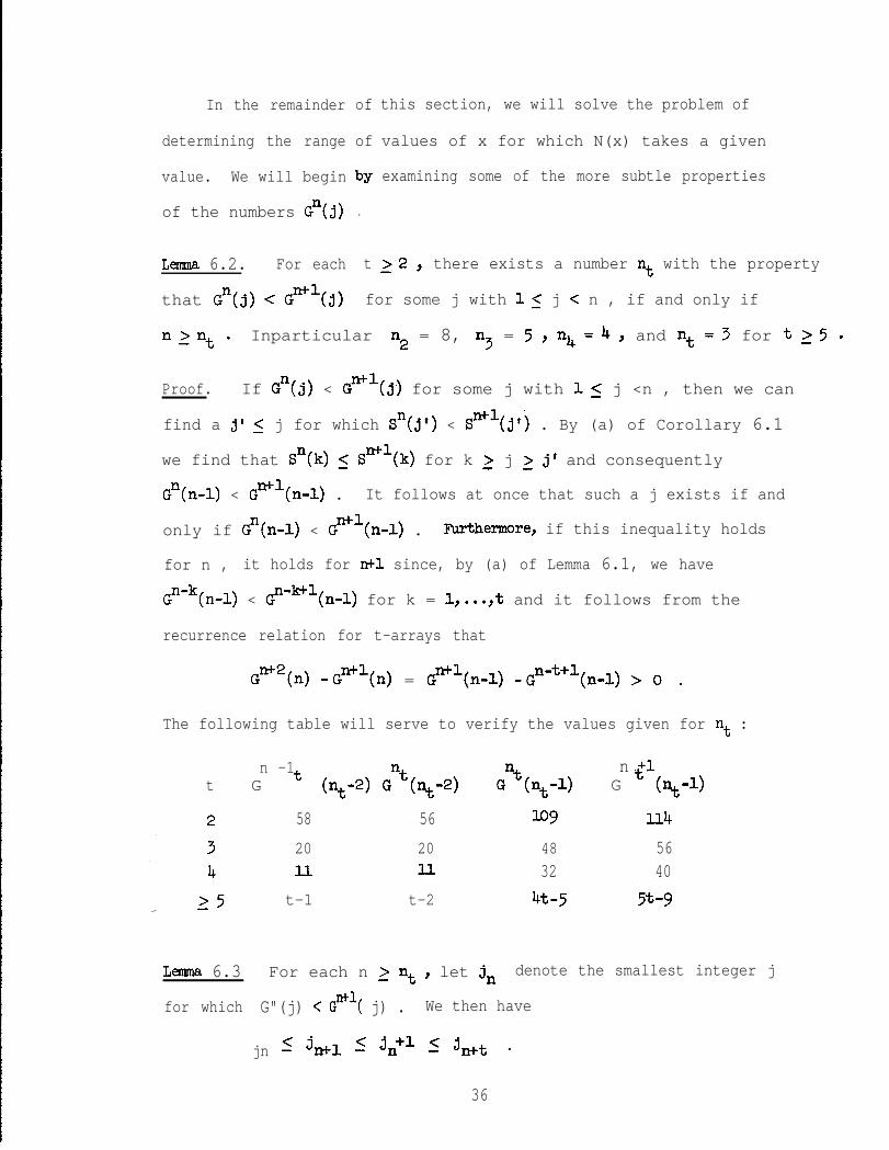
The following table will serve to verify the values given for nt :
n -1 n +lt G t (nt-2) ntG bt-2)
ntG (nt-l> G t (nt-1)
lemma 6.3 For each n 2 nt ) let jn denote the smallest integer j
for which G"(j) < GM'< j) . We then have
58 56 lo9 xl.4
20 20 48 56ll u 32 40
t-1 t-2 4t-5 5-t-9
jn ,< j,, 5 jn+l ,< 3,t l
36

Proof. First we will show that jn 5 jn+, . Assume that for some
k < jn we have GM1 (k) < GM2(k) . We may write/
Gn+l(k) -Gn(k) = Gn(k-1) -Gn-t(k-l)
= ($+'(k-1) -Gn-t+l(k-l))
+ @(k-l) -Gn+'(k-1))
+ (Gn-t+l(k-j) - Gnot(k-1)) .
The first parenthesized term is equal to crrc2(k) -Gn+'(k) and is therefore
positive. The second term is nonnegative since k < jn . Since
Gn+'(k) < Gm2 (k) it follows from the recurrence relation for t-arrays
that G*l-m(k-l) < G*2-m(k-l) for some m with 15 m 5-t . From (a)
of Lemma 6.1 it follows that Gn-t(k-l) < Gnot+'(k-l) so the last
parenthesized term is nonnegative. We have therefore shown that
Gn(k) < G*'(k) which contradicts the minimality of jn .
n+l .Since Gn(jn) < G (J )
til( jn+l) < Gti2( jn+y)
, we may show as in the proof of Lemma 6.2
that G and therefore jn+l-< jn+l . Finally,
since Gn+t(j,t) < G*t+l(j,t) , it follows that
tit-k .(J&-l)
ntt+l-k ,G < G (J tit-l) for some k with 1~ k ,<t .
Consequently,jn 5 jmtmk 5 $,.&� l
This completes the proof. c1
. Lemma 6.4. Define the numbers Nt by N2 = 19 , N3 = 6 , and Nt = nt
for t 2 4 l If n ,>Nt and j 20 , then
2Gn(j) ,< Gn(j+l)+ Gn+l(j-l) .
Proof. We will show that the above inequality holds for all but finitely
many values of n _>l and j ~0 . The condition on n is sufficient
to exclude these exceptions. We define the t-array D by
37

D%> = Gn(j+l)+Gml(j-1) -2Gn(j) .
It is not difficult to verify that the nonzero elements of the
initialization region for D are
Do(j) = (t-1)j -t for j 21 and
D"(-1) = 1 for l-t $3 10 .
We observe that Do(l) = -1 is the only negative element for the
initialization region. Tables 6.1(a), 6.1(b), and 6.14~) each display
a portion of the t-array D for t 2 4 , t = 3 , and t = 2 , respectively.
By3nspecting these tables, it is clear that there are no negative values
of Dn(j) with n 20 other than those displayed. Since the negative
entries only appear in the columns for which n < Nt ) it follows that
Dn(j), 2 0 when n>Ntg cl
Theorem 6.2. If nLNt and if we define
Cn = Gn(jn) -Gtil(jn-1) ,
then the following are true:
(4 S”(j,) 5 cn 5 S"(j,+l) )
(b) Sml(jn-l) ,< cn < Swl( j,> ,
(4 v”(c,> = ~?c,) >
(d) Vn(cn+l) > ?+'(c,+l) if cn < sn ,
( >e cn<Ctil '
38

Proof. From the definition of jn we know that $(j,-1) 2 Gn"(jn-1) .
We therefore have /
sn(j,) = Gn(jn) - G%,-1) ,< G"( j,) - Gtil( j,-1)
= Cn < G*'(j,) -GH1(jn-1) = S*'(j,) .
From Lemma 6.4
Cn = Gn(jn) -G?j,-1) ,< G"(j,+l) -G"(j,) = S"(j,+l) .
Also from Lemma 6.4,
s*l(jn-l) = Gtil (3 n-1) - GmT(jn-2) 5 Gn(jn) - Gwl(jn-l) = cn .I
This completes the proof of (a) and (b).
From (a) and (b) we have
v”(c,) = (j,+l>c, - Gn(j,)
= j,G%,) - (j,+l)G*'(j,-1)
= jc -Gn n = v"fl(cn)
which is (c). TO prove (a> we first observe that from (a) and (b) we
have Jlfl(c,+l) -pl(cn) = jn and Vn(cn+l) -?(cn) 2 jn+l if cn < Sn .
From (c) it follows that
fl(cn+l) -vn+l(cn+l) > l+F(cn) -F+l(c ) = 1 .n
. BY Lemma 6.3 we have jn 5 jtil so by (a) and (b)
Cn < StilCj,) 5 Sml&+,) < Cm1-
which is (e). This completes the proof. 0
Corollary 6.2. cn + m as n --) 00 .
Proof. This follows from (e) and the fact that cn is an integer. c3
39

For each t 12 , we define the sequence L&,.** as follows:
If t_>3, then we let Ln = S" for n < Nt and Ln = cn for n 2 Nt l
If t=2, then we let Ln = Sn for n 5 15 ) L16 = 2573 J L17 = 3954 t
L18 = 6527 , and Ln = cn for n zN2 = 19 .
Theorem 6.3. The sequence Ll,L2,... is strictly increasing and has
the property that p1(x) 2 v"(x) if and only if x 5 Ln .
Proof. First we will show that the sequence is strictly increasing. We
1 already know that sn < SW1 for all n 11 and that cn < cntl for
all nLNt. These observations leave us with only a few special cases
to consider.
When tz3, we must show that when n = Nt-1 , we have
Sn =Ln <Lrrel= ctil. When t ,> 5 we may show from the appropriate
t-arrays that S2 = 2t-1 and c3 = 3t-2 so that Ln < Lwl since
Nt=3. When t = 4 , we have Nt = 4 and L3 = S3 = 13 < 22 = c4.= L4 l
For t = 3 , we have Nt = 6 and L5 = S 5 = 31 < 32 = c6 = L6 . For the
L 2-5remaining special case t = 2 , we have 15 = = 1597 < 2573 = L16 9
L16 <L17 < L18 ' and L18 = 6527 ~10488 = cl9 = ~~~ .
To prove the second part of the theorem, it is sufficient, in view
of Theorem 6.1, to show that p1(L,) > Vn(Ln) for all n ,>l and that
J"l(Ln+l) < Vn(Ln+l) whenever Ln < Sn . If n < nt , then
Gn(j) 1 Gtil(j) for all j with 0 5 j <n , so by Theorem 6.1, we have
We also note that Ln = Sn for n < nt . When
">Nt 9 then everything follows from Theorem 6.2. Since nt = Nt forF., t_>4, this proves the result for t 2 4 . To extend the result to the
i case t = 3 , we observe that in this case we have L = S5 andL 51
Iv5@,)
6= 107 <108 = v (Lo) l
i
40
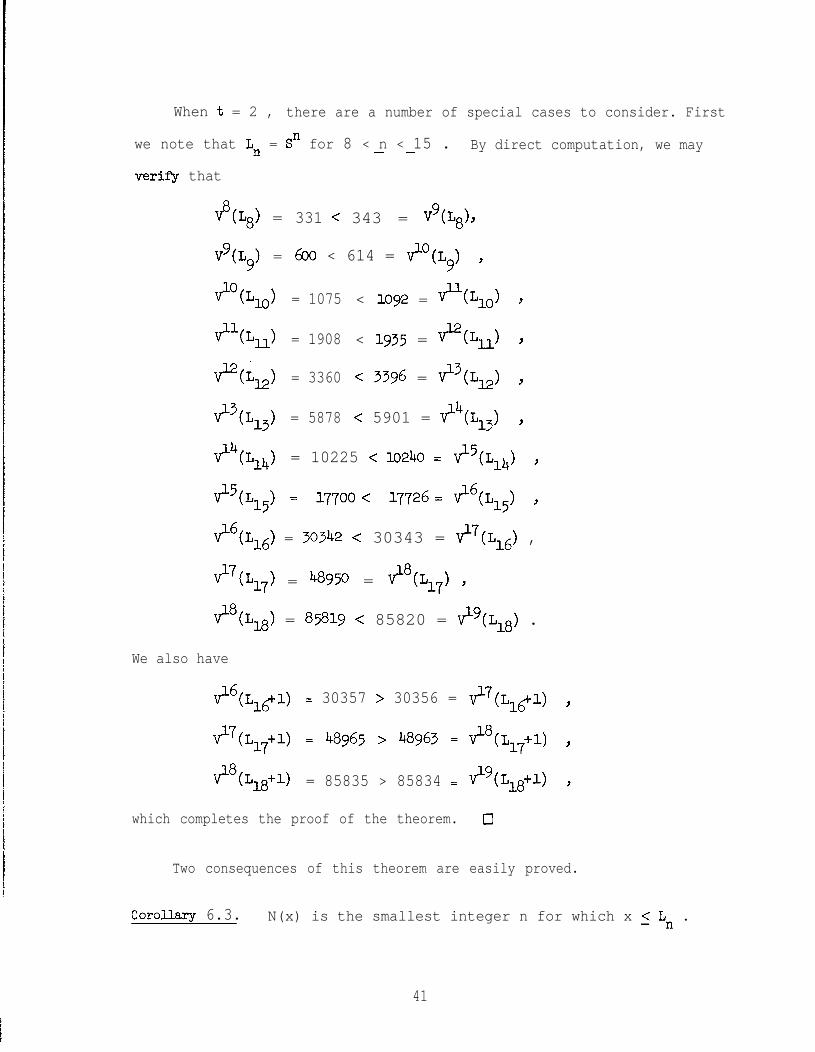
When t = 2 , there are a number of special cases to consider. First
we note that Ln = Sn for 8 < n < 15 .- - By direct computation, we may
verif'y that
v8 =(9 331 < 343 = vg(+3) 9
V9(Lg) = 600 < 614 = so@,) t
+"(L,) = 1075 < 1092 = +TL,)
v%,) = 1908 < 1935 = JJ=(Q
v=(i,) = 3360 < 3396 = I+'(L~~)
$3(L13) = 5878 < 5901 = $4(L13)
94(L14) = 10225 < 10240 = $5(L141 Y
$5(L151 = 17700 < 17726 = +TL15) .,
ti6(L16) = 30342 < 30343 = v17(L16) ,
~7@17) = 4-8950 = *8(L17) )
?8(L18) = 85819 < 85820 = $9(L18) .
We also have
P(L&+l) = 30357 > 30356 = ti7(Ll@
+Q7 L17+1) = 48965 > 48963 = $(8 L17+u
+Q8 L18+1) = 85835 > 85834 = $9( L18+1)
which completes the proof of the theorem. 0
Two consequences of this theorem are easily proved.
Corollary 6.3. N(x) is the smallest integer n for which x ,< Ln .
41

Coronary 6.4. If V"(X) ,< p'(x) ) then v"'(x) < v"'+'(x) for all
Remark. Corollary 6.4 answers in the affirmative a conjecture of Knuth
([5], Exercise 5.4.2-15).
Table 6.2 provides the values of L- for t = 2,...,7 and
n = l,...,lg . Since
provide a very simple
such a table is easily prepared, we are able to
dispersion algorithm.
Algorithm 6.1. OptimaJ Polyphase Sort for x Strings.
Step 1. Find the smallest n for which x ,< Ln .
Step 2. Choose a j for which Sri(j) 5 x 5 S"(j+l) .
Step 3. Find integers xl,...,xt for which x = xl+ . ..+xt and
SF(j) 5 xi 5 SF(j+l) for i = l,...,t .
Step 4. For each i = l,...,t write xi strings to tape i .
Step 5. Use Algorithm 4.3 to perform the polyphase merge on the
distribution xl,...,xt starting at stage n .
Remarks. Since Steps 2 and 3 of the above algorithm and Steps 1 and 2 of
Algorithm 4.3 both require tables of the numbers q(j) 9 some of the operations
of these steps can be combined. The above algorithm should be compared with
Shell's opf~imum dispersion algorithm [8] which is directed by a table of
numbers closely related to the numbers Ln . The functions c(x) share
many of the properties of the function J‘(x) and most of the results of
this section can be carried over to these functions. Unfortunately, the
analogues of the numbers jn are in general different for each i ;
otherwise the next section would not have to have been written.
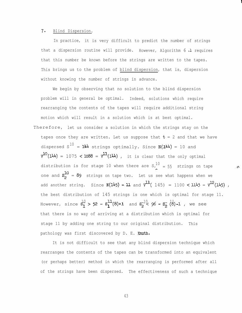
7*
that
that
This
Blind Dispersion.
In practice, it is very difficult to predict the number of strings
a dispersion routine will provide. However, Algorithm 6 .l requires
this number be known before the strings are written to the tapes.
brings us to the problem of blind dispersion, that is, dispersion
without knowing the number of strings in advance.
We begin by observing that no solution to the blind dispersion
problem will in general be optimal. Indeed, solutions which require
rearranging the contents of the tapes will require additional string
motion which will result in a solution which is at best optimal.
Therefore, let us consider a solution in which the strings stay on the
tapes once they are written. Let us suppose that t = 2 and that we have
dispersed S10
= 144 strings optimally. Since N(144) = 10 and
vlO(l44) = 1075 <1088 = vyl44) , it is clear that the only optimal
10distribution is for stage 10 when there are S, = 55 strings on tapeA
one and SF = 89 strings on tape two. Let us see what happens when we
add another string. Since N(145) =.ll and $l( 145) = 1100 ~1143 = $'((145) ,
the best distribution of 145 strings is one which is optimal for stage 11.
10 ilHowever, since Sl > 52 = Sl (S)+l 10 11and S2 < 96 = S2 (8)-l , we see
that there is no way of arriving at a distribution which is optimal for
stage 11 by adding one string to our original distribution. This
pathology was first discovered by D. E. Knuth.
It is not difficult to see that any blind dispersion technique which
rearranges the contents of the tapes can be transformed into an equivalent
(or perhaps better) method in which the rearranging is performed after all
of the strings have been dispersed. The effectiveness of such a technique
43

depends on how close the distribution, prior to rearranging, is to an
optimal distribution. We remark that one kind of rearrangement which
incurs no extra cost is that of renumbering the tape units. Theorem 9.3
shows that a monotone distribution provides the best renumbering possible.
However, since the distributions which we will consider will be monotone
or can be made monotone, we will have no use for this technique.
In the remainder of this section, we will construct a nearly optimal
blind dispersion technique which requires no tape rearrangement. This
*dispersion technique can be used by itself or in conjunction with some
rearrangement algorithm.
Supposethat n->Nt . We define m(n) to be the largest integer
m for which jm = jn . From Lemma 6.3 we see that m(n) < ntt and
that jm = jn for n srn rm(n) . For i = l,...,t we define
BY = min{St(j,) \ n ,< m 5 m(n)+11
and
Bn = B; + . . . + Bz .
for l_<i_<t ;
Theorem 7.1. For n 2 Nt we have
(a) By 5 By1
(b) By ,< B; < . . . 5 B; ;
(c) Sr(j,-1) ,< Bi 5 @,) for lli,<t ;
(a) S!f%n-l) ,< Bf ,< ST'(j,) for lsist ;
- (e) Bn ,< cn < Bmt .
Remark. Statements (c) and (d) imply that the distribution $Yn
. . ..Bt
is opbima.l for both stage n and stage ntl .
44

r
Before we prove the theorem we require a lemma:
Lemma 7.1. If n 2 Nt , then for i = l,...,t we have
S~�(jn-l) ,< Sf&$.☺ l
Proof. We will begin by showing that for n > 1 we have
(7-l) S?(j) -Sml(j-1) > Gn(j-1) -Gml(j-1)1 i
with only finitely many exceptions. We define the t-arrays Ai for
i = l,...,t and D by
A!&0 = S:(j) -S"'(j-1)
D"(j) = #(j-l) -Gtil(j-1) .
It is not difficult to verify that the nonzero elements of the initialization
regions for the t-arrays Al, . . ., 4t are
i-t .Ai (J) =l for l<i<t and j_>O ,
Ai-t-l .w = -1 for l.< i <t and j,>l Y
A:(j) = -1 for l<i<t and j 12 , and
= A;(l) =l.
Aho, the nonzero elements of the initialization region for the t-array D
are
Do(j) = t -(t-1)j for j 21 .
Tables 7.1(a) to 7.1(g) each display portions of the t-arrays Ai-D for
various ranges of t and i . By inspection, we see that the only
negative entries outside of the initialization region are those displayed.
Except in the case t = i = 2 , we see that (7.1) holds for all n 2 Nt
45#

and i = l,...,t . From the definition of jn , we see that
Gn(jn-1) 2 Gml(jn-1) and therefore by (7.1) we have Si(j,) 2 Srl(jn-1) .
In the exceptional case we have n = Nt = 19 and j19
= 15 so we may
verify directly that Sig(15) = 6050 > 5270 = S34) . This capletes
the proof. 0
Proof. of Theorem 7.1. If jn = jn+l , then m(n) = m(n+l) so that (a)
is obvious. If this is not the case, then by Lemma 6.3, we mmt have
.JIl+l = jn+l so that SiYj,) 5 Sffl(☺wl) l Also, since m(nt1) ,<n+t ,
we see that Sin+l(jn) 5 S:(J,1) for n+2 < k < m(n+l)+l ; this follows- -
from the fact that Sy'(j,) is a term of the t-sum which computes
We have therefore shown that .Bf 5 Si*'(j,) 5 BT1, which
is (a). Statement (b) follows at once from the fact that
S:(j) 5 . . . 5 s,"(j) for all n ,>l and j 21 .
To prove (c) and (d) we first observe that the definition of By
implies that BF ,< Si(j,) and B; #(j,) . It is also clear that
S~~~n-l) ,< S&J and Syl(jn-1) 5 Sf;fl(j,) . From Lemma 7.1, we have
S”l(jn-l) 5 S!$,) . Finally, by reasoning sjmilar to that used in the
above paragraph, we have Sy(j,-1) 5 St(j,) for ntl < k < m(n+l) and- -
SF'&-1) 5 S:(j,) for n+2 < k <m(n)+1 if m(n) > n . From these- -
inequalities, it follows at once that Sy(j,-1) ,< Bi and that
Sy'(jn-1) 5 By which completes the proof of (c) and (d).
By (c) we have B" ,< Sn(jn) 5 cn . If we let n* = m(n)+1 , then it
is clear that j,, = jn+l , jnf 1 = jn , and n* < n+t . Therefore, by
46

(a) and (c) we have
n* n*Cn < 'nt-1 < S (jnt-l> = S (j,& < B
n* <Bn+t- -
which establishes (e) and completes the proof of the theorem. 0
From the theorem, two important properties of the distributions
B;Y . . ..Bt"are apparent. First, we may arrive at the distribution
II+1Bl
II-+1Y l . vBt
by simply adding strings to the distribution B;Y . . ..I$ .
Second, if we are dispersing for stage n and we reach the distribution
J$ . . ..Bt , then we may begin dispersing for stage n+l since the
distribution is optimal for both stages. Clearly we can base a blind
dispersion algorithm on these properties of the numbers By . However,
since we will be making several refinements, it is of value to examine
the general structure of such an algorithm.
We define a quota scheme for polyphase dispersion to be a family of
nonnegative integers Q",Q$ . . ..&tn , n = 1,2,... which have the following
properties for _n>l and l,<ist:
Qf L S; , Q; 5 QT’ Y Qn _<Qtil I
Qn ,< QT + . . . + Qt , and Qn 4 03 as n 3 03 .
Following is the dispersion algorithm which is directed by the quota
scheme. The counters xl, . . ..x+. contain the numbers of strings which have
been'written to tapes l,...,t . Upon completion, the values of
⌧-1, l �9X* and n are the parameters for initializing Algorithm 4.3.
47
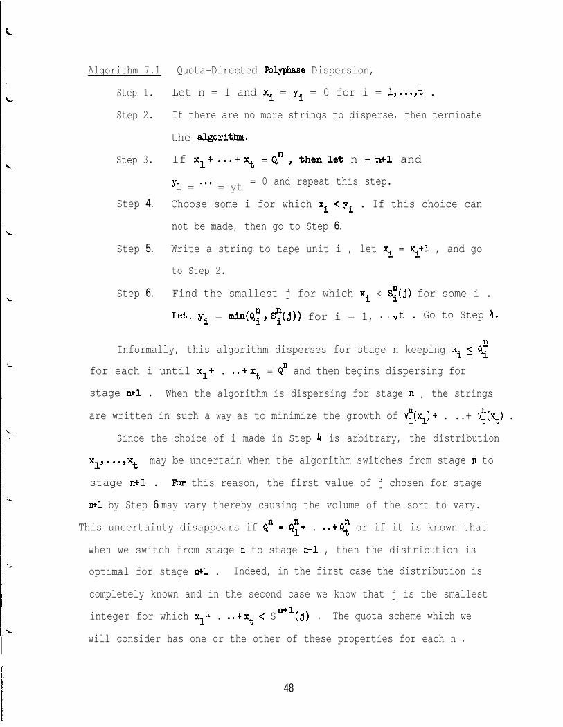
Algorithm 7.1
Step 1.
Step 2.
Step 3.
Step 4.
Step 5.
Step 6.
Quota-Directed Polyphase Dispersion,
Let n = 1 and xi = yi = 0 for i = l,...,t .
If there are no more strings to disperse, then terminate
the algorPthm.
If xl+...+xt =Qn, thenlet n =n+l and
y1 = "* = yt = 0 and repeat this step.
Choose some i for which xi <yi . If this choice can
not be made, then go to Step 6.
Write a string to tape unit i , let xi = xi+1 , and go
to Step 2.
Find the smallest j for which xi < SF(j) for some i .
Let. Yi = min(Q$S~(j)) for i = 1, . . ., t . Go to Step 4.
nInformally, this algorithm disperses for stage n keeping xi 5 Qi
for each i until xl+ . ..+xt = Qn and then begins dispersing for
stage n+l . When the algorithm is dispersing for stage n , the strings
are written in such a way as to minimize the growth of <(xl)+ . ..+ <(x+,) .
Since the choice of i made in Step 4 is arbitrary, the distribution
x~'*-,x~ may be uncertain when the algorithm switches from stage n to
stage ntl . Ear this reason, the first value of j chosen for stage
n+l by Step 6 may vary thereby causing the volume of the sort to vary.
This uncertainty disappears if Qn = Qr+ . ..+< or if it is known that
when we switch from stage n to stage ntl , then the distribution is
optimal for stage *l . Indeed, in the first case the distribution is
completely known and in the second case we know that j is the smallest
integer for which xl+ . ..+xt < Sntl(3) . The quota scheme which we
will consider has one or the other of these properties for each n l
48
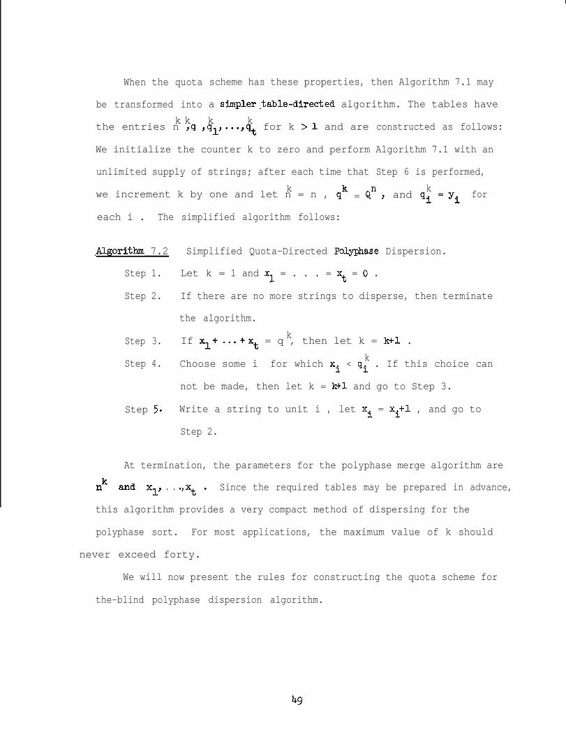
When the quota
be transformed into
scheme has these properties, then Algorithm 7.1 may
a simplertable-directed algorithm. The tables have
k k k kthe entries n ,q ,ql,..~,qt for k >l and are
We initialize the counter k to zero and perform
unlimited supply of strings; after each time that
constructed as follows:
Algorithm 7.1 with an
Step 6 is performed,
kwe increment k by one and let n = n , qk = Qn Yk
and qi =yi for
each i . The simplified algorithm follows:
,Algorithm 7.2
Step 1.
Step 2.
Step 3.
Step 4.
Step 5*
Simplified Quota-Directed Polyphase Dispersion.
Let k = 1 and x1 = . . . = xt = o .
If there are no more strings to disperse, then terminate
the algorithm.
kIf xl+...+xt = q , then let k = Hl .
Choose some ik
for which xi < qi . If this choice can
not be made, then let k = k+l and go to Step 3.
Write a string to unit i , let xi = xi+1 , and go to
Step 2.
At termination, the parameters for the polyphase merge algorithm are
nk and x1, . . .,xt ' Since the required tables may be prepared in advance,
this algorithm provides a very compact method of dispersing for the
polyphase sort. For most applications, the maximum value of k should
never exceed forty.
We will now present the rules for constructing the quota scheme for
the-blind polyphase dispersion algorithm.
49

1.
2.
3.
4.
If nzNt and if By < ST(j,) for some i , then we let
Qn = Bn and Q; = B; for iv= l,...,t .
If n zNt and if Bf =
Q; = min(Sy(jn+l) ,
for i = l,...,,t and we
S!$j,) for each i , then we let
Sy'(j,) , By?
let
Qn = min(cn,&:+ . ..+c%. .
If t 2 3 and l_<n <Nt , then we let
Qn = Sn and Q; = S; for i = l,...,t .
If t= 2 and n<Nt = 19 then we let
Qn = Sn nand Q:=Si for n 515 and i = l,...,t
and, in addition, we let
Q16
= L16 = 2573 , Q17 = 3845 , Q18 = $3 = 6527 ,
16Ql = $915) = 986 , Qk6 = si6(15) = 1596 ,
17Ql = $8(13) = 1383 , Qi7 = sk7(14) = 2462 ,
18Ql = si8(16) = 2567 Y Qi8 = si8(16) = 4163 .
. To show that these rules define a quota scheme, we will being by showing
that for n 2 Nt , we have
Bn 5 Qn ,< B@-I. and B; 5 Q; ,< By1 for i = l,...,t l
These relations are obvious when Rule 1 is applied. If Rule 2 is applied
instead, we have, from Theorems 6.2 and 7.1,
50
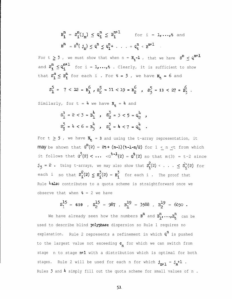
B; = Sy(jn) ,< Qy 5 By' for i = l,...,t and
Bn = sn( j,) 5 Qn 5 Q;+ . . . + Q; < Bml .
For t 2 3 , we must show that when n = Nt-1 ,
II+1and Sy -<Qi for i = l,...,t . Clearly, itn n
that we have Sn ,< Qml
is sufficient to show
that Sl,< By for each i . For t = 3 , we have I$ = 6 and
5Sl = 7 < 12 = B; , S; 6==<lg=B2 , S; 6= 13 < 27 = ~~ .
Similarly, for t = 4 we have Nt = 4 and
3sl
4=2<3=Bl, S; =3<5=Q;,
S33=4<6=~;, sz =4<7=Q; .
For t 2 5 , we have Nt = 3 and using the t-array representation, it
may be shown that Gn(2) = 2t+ (n-1)(&l-n/2) for 1 < n <t from which- -
it follows that G3(2) < a=. <Gt-1(2) = Gt(2) so that m(3) = t-2 since
j3=2. Using t-arrays, we may also show that E?(2) < . . . t5 Si(2) for
each i so that S:(2) ,< S;(2) = B: for each i . The proof that
Rule 4 also contributes to a quota scheme is straightforward once we
observe that when t = 2 we have
S151 = 610 , Sk5 = 987 , Big = 3588 , Big = 6050 .
We have already seen how the numbers Bn and BF,...,Bt can be
used to describe blind polyphase dispersion so Rule 1 requires no
explanation. Rule 2 represents a refinement in which Qn is pushed
to the largest value not exceeding cn for which we can switch from
stage n to stage n+l with a distribution which is optimal for both
stages. Rule 2 will be used for each n for which j,, = jn+l .
Rules 3 and 4 simply fill out the quota scheme for small values of n .
51

The special assignments in Rule 4 were chosen subjectively to insure
reasonably good performance.
If we are dispersing using the quota scheme just described, it is
clear that when the number of strings x is large, then we will switch
stages with a distribution which is optimal for both stages. Consequently,
the volume of the sort will be vN"")(x) for some integer N*(x) when x
is sufficiently large. Since Qn ,< cn for n ,>Nt , it is clear that
N'(x) 2 N(⌧) l On the other hand, since cn <Bnt‘t
SQn+t , we see that
N? (x) < N(x)+t .
The blind polyphase sort which we have described is almost as good
i as the optimal polyphase sort of Algorithm 6.1, when the number of strings
is in the range of the size of most applications (say, less than a thousand),
the two sorts are almost always equivalent. When the number of strings
is large, it can be shown that the two algorithms are equivalent infintely
often. Indeed, this happens for S"(j,) strings every time that
.Jn+l = jn+l . In the next section we will show that the two algorithms
are also asymptotically equivalent.
Example 7.1. Table 7.2 displays a portion of the simplified quota scheme
for the case t = 4 .
52

8. Assmptotic Performance.
In this section, we will study the performance of the algorithms
which we have described when the number of strings is large. There are
two volumes which we are interested in estimating. First there is the
volume of the optimal polyphase sort of Section 6,
v(x) = vN’“‘(x) ,
and, second, there is the volume of the blind polyphase sort, when x is
large, this is
V�(⌧) = vN��+X) l
We wiU. show that when x is large that both of these volumes are
asymcptotically equal to
x l o x + 1Qt 2xlogtlogt x+ o(x) .
The reader who is not familiar with asymptotic methods may find [1] or
the first chapter of [4] to be helpful.
Our startingpoint is an interesting connection between the movement
numbers and the theory of probability. I&?-t YlJY2J l **be independent
random variables which each take on the values 1,2,...,t with equal
probability t -1 . Simple calculations will show that each yi has an
expectation ~1, = (t+1)/2 and a variance o2 = (t2-1)/12 . For positive
integers m and k we define
(8J) p(m,k) = prob(yl+ . ..+Yk = m) .
Lemma 8.1. For n ,>l and j >l , we have <( )3 = tjp(n,j) .
Proof. Let q(z) = z+z2+ . ..+zt for the real variable z . We will
begin by showing that
53
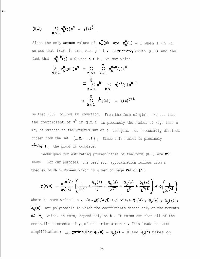
(84 C $(j)z” = q(z)’ .n>l
Since the only nonzero values of4)(1 are g( )1 = 1 when 1 <n <t ,
we see that (8.2) is true when j = 1 . Furthermore, given (8.2) and the
fact that = 0 when n 5 k , we may write
C <(j+l)Z = Cn>l
4; $-"(j)z"nil k=l
t= c zk ck=l n_>l
$Ok(j > znok
t=‘c kz q(z)j = ,(z)j+lk=l
so that (8.2) follows by induction. From the form of q(z) , we see that
the coefficient of zn in q(z)j is precisely the number of ways that n
may be written as the ordered sum of j integers, not necessarily distinct,
chosen from the set El 2Y ,**.t t3 lSince this number is precisely
QkWl , the proof is complete.
Techniques for estimating probabilities of the form (8.1) are well
known. For our purposes, the best such approximation follows from a
theorem of C. G. Esseen which is given on page 241 of [3]:
p(m,k) =e-s2/2
J&-
where we have written s =. b-d/d and where Q1(S) Y Q2(s) Y Q3(s) Y
Q4(5) are polynomials in which the coefficients depend only on the moments
of Yi which, in turn, depend only on t . It turns out that all of the
centralized moments of yi of odd order are zero. This leads to some
simplifications; in PLIrTtic- Q1(s) = Q3(s) = 0 and e,(s) takes on
54

the simplified form c(s4
- 6s2+ 3) in which c depends only on t .
Using the estimates
2ems I2 = 1 - 4; s2 + o(s ) ,
Q2(s) = 3c+o(s2+ s4) ,
we obtain the approximation
p(m,k) = -
which may be written in the form
p(m,k) = -jL(&+&(3c~~))+o(~~) l
To simplify subsequent calculations, we will use the symbol pn(z) to
represent generically an n-th degree polynomial in z in which the
coefficient of 2 is positive and in which all of the coefficients
are functions only of t . Two distinct appearances of the symbol in
the text need not represent the same polynomial. With this convention,
we now have
(8.3) p(m,k) = up=& - -& q” - $1 + 0 (W) ’
Lemma 8.2. We have
(8.4) fit-jMn-(j) = L - 5 aJ,(n-pj)+Ou 2nr
(I+ y8) .
55

Proof. From the last, two formulas of (3 .l), we have
so that
M"(j) = t$-'(j-l)+ (t-l)go2(j-l)+ . ..+qot(j-1) .
Therefore, by Lemma 8.1, (8.3), and the facts that
we have
t-j#( j)t
= C (t-i+l)t-j I$-i(j-l)i=l
= t-ltC (t-i+l)p(n-&j-l)i=l
t-l t= / C (t-i+l) -
&xj i=l - it1
which is easily reduced to the form (8.4). 0
Lemma 8.3. We have
(8.5) 6 t'j$(j) = 11 - -t2
o&T (t-l)2 j
56

Proof. From our definitions we have
.
Gn(j) = 5 S"(j)
.
= 5kX I?(i)
k=l k=l i=l
. j-l= h (j-k+l)M?k) = c (k+l)#(j-k) .k=l k=O
Using this formula and Lemma 8.2, we obtain
t-'Gn( j) =j-lc t-j(k+l)Mn(j-k)
k=O
j-l= c tok(ktl) I-
P2b - pj + pk)
k=O - - (j-k)3/2 )
j-lc tok(k+l)
k = O
In order to simplify the above approximation, we need to be able to
estimate sums of the form
j-l kaS(a,b) = c
k=O (j-k)btok
for. a = 0,1,...,9 and b = l/2,3/2, 512 . Let us write m = L/j]-1 .
If j is sufficiently large, then we will have ka < (3/Z) k for all
k >m and a = 0,1,...,ll . From the binomial expansion, it is clear
that for k <m , we have
1 1 bk
(j-k)b = jb-+jb+l+O
.
It is also clear that
E kat-k= s(a)+O((3/2t)m)
k=O
where
57

s(a) = fi katok .k=O
We therefore have
s(a,b) = .t, ($+ b$;l)t-k+ k;;l (j;)b t-k
since the second sum is 0((3/2t)m) and the last sum is O(l/jH2) .
Since (3/2t)m
error estimate
from the facts
s(o)
‘Corollary 8.1.
is O(l/jM2) for each b , we may replace the above
by O(l/jM2) . The conclusion of this 1-a now follows
that
= t/(t-1) and s(l)
If n-pj = O(1) , then
3fi to'c"(j) = d!L- " +
adz (t-Q2
Proof. This is a simple consequence of the lemma.
= t/(t-l)2
0 IL( J3 l
. cl
0
CoroUary 8.2. Let jn be defined as in Section 6, we then have
n_-pjn = O(1) .
Proof. We recall that jn is the smallest integer j for which
Gn(j) < GM'(j) . From the estimate (8.5), we obtain
6 toj(G*'(j) - G"(j)) =Pl(n - d)
j
58

With Pl understood to
number which satisfies
pl(n-pj) is less than
n andif j_<LaJ-1, then
be the pl appearing above, let a be the real
= 0 . If j ,> ral+l , then clearly
some negative quantity which is independent of
quantity which is independent
LaJ -1 < j < [al+1 , we have- -
becomes O(jo2) so the first
PJn - pj) is larger than some positive
of n . For 3 in the range
n - pj = o(1) and the error estimate above
term of the estimate dominates. It follows
that jn lies within this range for large n and the proof is complete. a
Theorem 8.1. v(x) =x10 x +1
Qt ~XlOgt logt x+ o(x) l
P r o o f . Let cn = Gn(j ) -c"'(j -1) be defined as in Section 6. Fromn n
Corollarys 8.1 and 8.2 it is easily shown that
.
(8.6) l/jntoJn cn = PaG & + O(jr;l) .
If x is sufficiently large, then for n = N(x) we have c~-~ < x 5 cn .
Let j be the unique integer for which S"(j) <x 5 Sn(j+l) . From
Theorem 6.2, it is clear that jn-l-ls j ,< jn . Using the formula
v(x) = (j+l)x -Gn(j)
we may write
. (8.7) V(X) -x 10~ x = x(j+l-10~ x) -Gn(j) .
From (8.6) we have
110~ cn = jn - 2 logt jn + O(1)
and therefore, since 0 < j- n-jn-l 5 IL 9
59

j+l-logtx < j+l-logt 'n-1
= j+'-jn+ 22r 10% jnml + 00)
,< &+1-j,+ 2ll,gt jn + O(1)
= 1~10~ jn + O(1) .
Similarly
j+l-10gt _x > j+l-logt cn = $ 10% jn + O(1)
and we have shown that
(8 41j+l-logt x =+ogt jn + O(1) .
comparing Corollary 8.1 and (8.6) we see that
G% > = O(Cnol) = o(x) .
From (8.8) and the fact that j,-2 < j s jn , we have
-1jn 10% x = l+O(j,-' 10% 3,)
so that
10% jn -10% 10% x = O(jillogt j,) = O(1) .
Putting everything together, (8.7) becomes
1V(x)-~10% x = Fxlogt jn+ O(x)
1= F x 10% 10% x + o(x)
and the proof is complete. D
60

Corollary 8.3. V'(x) = x logt x +
Proof. In Section 7 we showed that
Theorem 5.3, it follows that
1F x logt logt x + o(x) .
N(x) < N*(x) < N(x)+t . From
0 ,< V’(x) - v(x) = ~'(x+x) -flex)(x) ,< (N'(x) -N(x))x 5 (t-1)x
so that V*(x) -V(x) = O(x) and the result follows from the theorem. Cl
It is well known (see Section 5.4.4 of [5]) that the best possible
volume for a merge sort which performs p-way merges is x logp x+0(x) .
For this reason, a tape sort with T tape units has an optimum volue of
x logTo x + o(x) since such a sort can perform at most T-l -way merges.
A tape sort with T tape units which has a volume asymptotic to
x lo&r-l x is said to be asymptotically optimal. Theorem 8.1 and
Corollary 8.3 imply that both the optimal polyphase sort and the blind
ply-phase sort are asymptotically optimal.
Remarks. The optimal polyphase sort appears to be the first known example
of an asymptotically optimal read forward tape sort. Other examples will
appear in [g]. Several asymptotically optimal read backward sorts are
known (see, for example, Section 5.4.4 of [5]) but these sorts have volumes
of the form x logT1 x+0(x) which is smaller than the volume we have
derived for the optimal polyphase sort. One wonders if the volume
x l o x + 1_ &c 2 x logt logt x + o(x) can be improved upon for read forward
sorts or whether it represents some theoretical minimum. A simplified
self-contained analysis of the optimal polyphase sort, which is probably
suitable for students, appears in [lo].
61

9. Concluding Remarks.
Two questions concerning the optimal poQ@ase sort
investigation. First there is the problem of estimating
remain open for
the smount of
time the algorithm spends waiting for tapes to rewind and second there
is the problem of optimizing the read backward polyphase sort.
The rewind time is significant since both the blind and the optimal
polyphase sorts perform large numbers of tape rewind operations. Of course
we may suppose that the total amount of rewinding corresponds to the volume
'of information moved. However, the polyphase merge rewinds two tapes
simultaneously so it is conceivable that a highly unbalanced situation
may arise in which one of the two tapes being rewound would be considerably
longer than the other. This might cause the total rewind ,wai.t time to
vary from the volume of the merge to twice that volume.
In the read bacbard polyphase sort, the tape units act as stacks
so the direction in which a string is written is reversed when the string
is moved. Therefore, strings which will be moved an odd number of times
must be written in the omsite direction from strings which will. be
written an even number of times. For this reason, strings are no longer
interchangable so the dispersion routine must concern itself with the
details of placing the dummy strings.
In this paper, we have limited the discussion to the traditional
polyphase merge in which the appointment of the output tapes is cyclic.
The polmhase merge, however, is just a special case of the class of
single-output read-forward merge algorithms. Some information about these
techniques can be found in the exercises for Sections 5.4.2 and 5.4.4 of [5].
It is known for example that in certain special cases, the optimal polyphase
62
sort can be beaten by other methods of merging. In [g] it is shown that
a large class of single-output read-forward merge algorithms also give
rise to asymptotically optimal sorting algorithms.
63

Acknowledgments
This paper would have been a pale shadow of itself had I not
encountered a preprint of the first half of [5]. Professor Knuth also
read an early draft of the paper and made several valuable suggestions.
This research was conducted while I was employed at Sperry UNIVAC in
Roseville, Minnesota, and began as a study of possible sorting
procedures for the DMS ll.00 Schema Description (DDL) translator which
I was then implementing. I am indebted to Mr. E. H. Moulton for many
valuable conversations and to Mr. A. G. Reiter, Dr. H. C. Gyllstrom, and
M. D. Thompson, for allowing me to pursue this subject when I should have
been doing something else.
64


References
The references given below consist of only those books and papers
which are referenced in the text. An extensive bibliography on computer
sorting has been prepared by R. L. Rivest and D. E. Knuth which appears
in Computing Reviews, vol. 13, no. 6 (June lg2), pp. 283-289.
ml
PI
c31
141
c51
161
171
Ku
191
[lOI
de Bruijn, N. G., Asymptotic Methods in Analysis, North-Holland,
Amsterdam, 1970, 200 pp.
Flores, I., Computer Sorting, Prentice-Hall, Englewood Cliffs, N. J.,
1969, 237 PP.
Gnedenko, B. V., and Kolmogorov, A. N., Limit Distributions for
Sums of Independent Random Variables, Addison-Wesley, Reading,
Mass., 1954, 264 PP.
Knuth, D. Em, Fundamental Algorithms, The Art of Computer Programming 1,
Addison-Wesley, Reading, Mass., 1968, 634 pp.
Knuth, D. Em, Sorting and Searching, The Art of Computer Programming 3,
Addison-Wesley, Reading, Mass., 1973, 722 pp.
Lynch, W. Cm, "The t-Fibonacci Numbers and Polyphase S~rting,~~
Fibonacci Quarterly, 8 (1970), pp. 6-22.
Sackman, B. S., and Singer, T., "A Vector Model for Merge Sort
Analysis, Fart I, Folyphase Merge Sort," unpublished paper presented
at the ACM Sort Symposium (November ig62), 28 pp.
Shell, D. L., "Optimizing the X&phase Sort," Comm. ACM, 14, ll
(November lgl), pp. 713-719, Corrigendum, Comm. ACM 15, 1
(January 1972), p. 28.
Zave, D. A., "A Note on Merge Sort Analysis," (in preparation).
Zave, D. A., "A Simplified Analysis of the Optimal Polyphase Sortyt
-(in preparation).
65
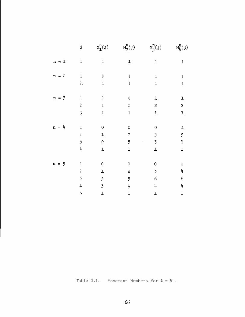
j.q(J) M;(j) .
g(J)
n=l 1 1 1 1
n=2 1
2.
0
1
1
1
1
1
1
1
n=3 1
2
3
0
1
1
0
2
1
n=4 1
2
34
n=5 1
2
34
5
Table 3.1. Movement Numbers for t = 4 .
66

j .n= -3 -2 -1 0 12 3 4 5 6 7
0 0 1 0 0
1 0 1 0 0
2 0 1 0 0
3 0 1 0 0
4 0 1 0 0
,5 0 1 0 0
6 0 1 0 0
7 0 1 0 0
0 0 0 0 0 0 0
1 1 0 0 0 0 0
1 2 2 2 2 1 0
1 2 3 5 7 8 7
12 3 6 IL 17 23
12 3 6 12 22 37
12 3 6 12 23 43
12 3 6 12 23 44
Table 3.2. S!!Jj) for t = 4 .
67
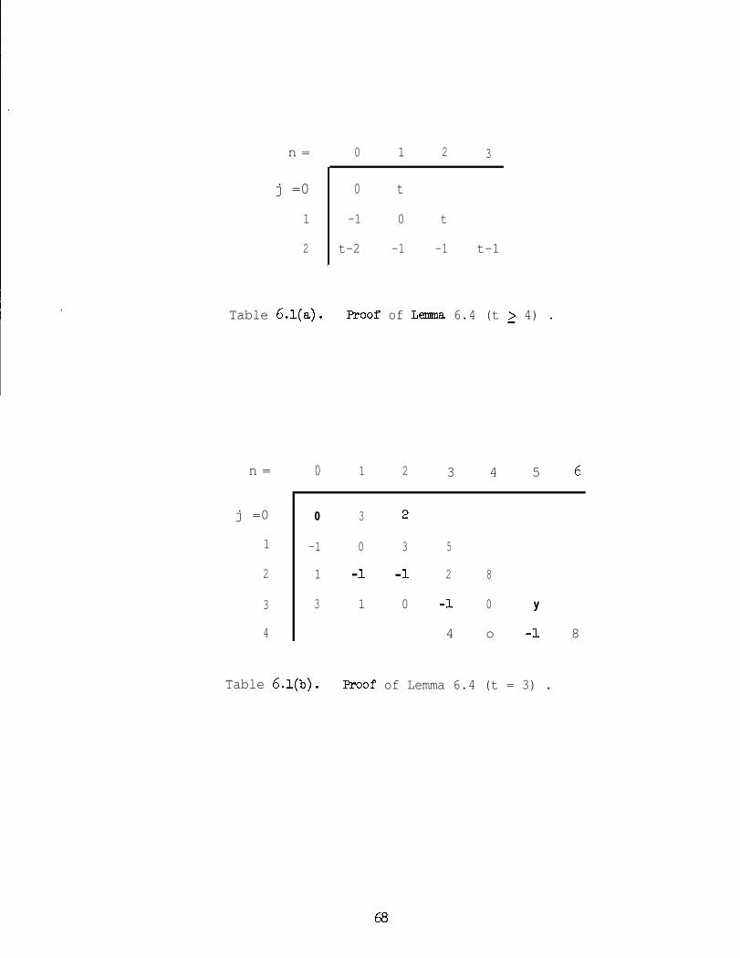
n = 0 1 2 3
j =0 0 t
1 -1 0 t
2 t-2 -1 -1 t-1.
Table 6.1(a). Roof of Lenma 6.4 (t 2 4) .
n = 0 1 2 3 4 5 6
j =0
1
2
3
4
0 3 2
-1 0 3 5
1 -1 -1 2 8
3 1 0 -1 0 y
4 o -1 8
Table 6.1(b). proof of Lemma 6.4 (t = 3) .
68
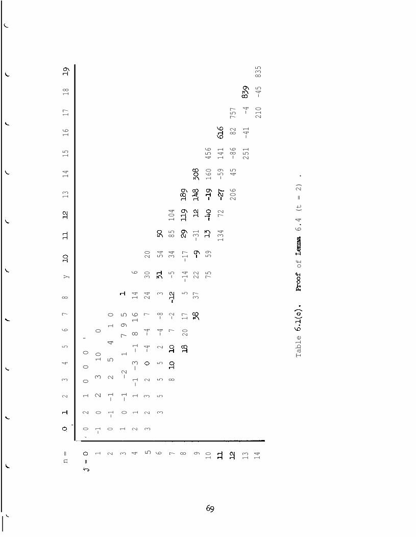
n=
.o1
23
45
67
8y
10ILL
1213
1415
1617
1819
It
j.
= 0 1 2 3 4 5
b
6 7 8 9 10 XL 12 13 14
0 -1 0 1 2 3
21
00
0'
02
3
10
0
-1-1
2
5
4
10
0-1
-2
1
795
11
1 -1 -3 -1 8 16
146
23
2o
-4-4
724
3020
35
55
2-4
-83
3154
50
810
107
-2-u
-534
85104
1820
175
-14
-17
29119
189
3837
22-9
-31
12148
308
7559
13-40
-19
160
456
134
72-27
-59
141
616
206
45-86
82757
251
-41
-4839
210
-45
835
Table 6.1(c).
proof of L- 6.4 (t = 2) .

n t=2 t 3= t=4 t 5= t=6 t=7
56
78
910
11
12
1314
1516
1718
19
2
3
58
1321
34
55
89144
233
377610
987
1597
2573
3954
652710488
3
5 7
9 13
17 22
31 34
54 75
95 108
172 243
279 358
534 455
819 11961634 1562
2400 4033
4958 5378
7028 6455
14952 18560
20582 22875
44898 64188
@w7 80858
4 5 6 7
9 11 13
13 16 1928 19 23
42 52 2 6
60 72 87
153 97 ll4
215 282 147268 385 167
778 480 639
JO33 554 7911248 1995 921
3909 2485 1016
4969 2900 4396
5840 10577 5250
19408 13096 5978
23917 15335 6498
27556 17028 30163
95802 69843 35027
Table 6.2. Ln for 2_<tL7 and lLn_<lg.
70

n = -1 0 12 3
3 =o
1
2
Table 7.1(a). ProofofLemma7.1 (tL4, i=t) .
0 1
-1 0 1 1
-1 t-2 -1 0 1
n = 1-t . . . 0 1
j =o 1 . . . 0
1 1 '..* -1 1
Table 7.1(b). ProofofLemma7.1 (t13, i=l) .
n = i-t-l i-t . -. . 0 12 3-~--r -1 1 0
---j =o 0 1 0 . . . 0
1 -1 1 0 . . . -1 1 1
2 . . . t-3 -1 LO 21
Table 7.1(c). Proof of Lemma 7.1 (t 2 4 j l< i <t) .
71

n = -2 -1 0 1 2
j = 0 0 1 0'
1 -1 1 -1 1
2I
-1 1 0 -1 1
Table 7.1(d). ProofofLema7.1 (t=3, i=2) .
n = -1 0 1 2 3 4 5 6
j =0
1
2
34
I0-1
-1
-1
-1
1
0 1 1 1
1 -1 0 2 3
3 0 -1 0 1 5
5 2 2 2 -1 0 6
Table 7.1(e) . ProofofLemma7.1 (t=3,i=3) .
72

n =
-1 o 12
3
4
5
6
78 y
10 u 12
$3
14
15
16
17
18
19
j= 0 1 2 3 4 5' 6 7 8 9 10 SL I2 13 14
0
0
0
0
0'0
-110
0
0
0
0
-lo
010
0
00
0
O-1
01
10
0
0
11
0
-1-l
1
21
00
2
2
2
1-l
-2
03 3
10
3
4
4
3
o-3
-2 3
6 4
1
7
8
7
3-3 -5
1 9
105
15 15
10
0-8 -4
1019
15
30 25
lo -8
-1.2
629
55 35
2-m
-6
9037
-3.8
327
34 3563
-26
29y8
19-44
3127
146
-25
-41
130
I21
-66
89
Table 7.1(f).
Proof
of Lemma 7.1
(t =
2 ,
i =
1) .

n=
-1012
34.5
67
8y
1011
1213
1415
16I
1718
1920
j= 0 1 2 3 4' 5 6 7 8 9 10 ll 12 13 14 15
01
-1 0
-1 0
-1 1
-1 2
-1 3 4
0
0
0
0
0
11
00
00
-1
12
10
0
0
-1-l
0
3
3
10
0
0
0 -2
-1
3
641
o
1 2 0 -2 -3
2 9m
51
2 4 3
2 -2 -5
-1 u
1915
6
6
6
o
-6
7
5
-7
1030
3421
12 13 12 5 -7
-13
440
.64
55
25 25 17
-2-20
-944
104
lly
5042
15-22
-29
35148
223
9257
-7-51
6183
149 50 -58 -45
199
-8
371
189
556
-103
144
745
191
-111
41899
80-7
0930
j
Table 7.1(g).
ProofofLema7.1 (t=2,i=2) .
. .-

i
i
L
c
L
k nkk
ql
1 1 4 1 1 1 1
2 2 7 1 2 2 2
3 3 9 1 2 2 2
4 3 13 2 3 4 4
5 4 21 3 5 6 76 4 22 4 6 7 8
7 5 30 4 7 9 10
8 5 34 4 8 IL 13
9 6 36 4 8 ll 13
10 6 71 10 17 21 2311 6 75 13 22 26 28
12 7 100 13 23 30 34
13 7 108 14 27 37 44
14 8 322 14 27 37 44
15 8 241 34 57 71 7916 8 243 44 77 92 100
17 9 338 44 78 101 11518 9 358 50 94 128 151
19 10 423 50 94 128 15120 10 455 50 100 144 17821 ll 472 50 100 144 17822 ll 1156 151 266 345 394
Table 7.2. Simplified Quota Scheme for t = 4 .c
75