OPTIMAL PLACEMENT OF STATCOM CONTROLLERS WITH ...
111
OPTIMAL PLACEMENT OF STATCOM CONTROLLERS WITH METAHEURISTIC ALGORITHMS FOR NETWORK POWER LOSS REDUCTION AND VOLTAGE PROFILE DEVIATION MINIMIZATION By Emmanuel Idowu Ogunwole (Student Number: 219098786) A DISSERTATION SUBMITTED IN FULFILLMENT OF THE REQUIREMENTS FOR THE DEGREE OF MASTER OF SCIENCE IN ELECTRICAL ENGINEERING, COLLEGE OF AGRICULTURE, ENGINEERING AND SCIENCE, UNIVERSITY OF KWAZULU-NATAL June, 2020 Supervisor: Prof. A. K. Saha
Transcript of OPTIMAL PLACEMENT OF STATCOM CONTROLLERS WITH ...

OPTIMAL PLACEMENT OF STATCOM CONTROLLERS
WITH METAHEURISTIC ALGORITHMS FOR NETWORK
POWER LOSS REDUCTION AND VOLTAGE PROFILE
DEVIATION MINIMIZATION
By
Emmanuel Idowu Ogunwole
(Student Number: 219098786)
A DISSERTATION SUBMITTED IN FULFILLMENT OF THE
REQUIREMENTS FOR THE DEGREE OF MASTER OF SCIENCE IN
ELECTRICAL ENGINEERING, COLLEGE OF AGRICULTURE,
ENGINEERING AND SCIENCE, UNIVERSITY OF KWAZULU-NATAL
June, 2020
Supervisor: Prof. A. K. Saha

i
CERTIFICATION
As the candidate’s Supervisor, I agree to the submission of this dissertation.
Signed: _________________________________
Signed: Prof. A.K. Saha.
Date: 29 June, 2020

ii
DECLARATION 1 - PLAGIARISM
I, Emmanuel Idowu Ogunwole, declare that
1. The research reported in this thesis, except where otherwise indicated, is my original research.
2. This thesis has not been submitted for any degree or examination at any other university.
3. This thesis does not contain other persons’ data, pictures, graphs or other information, unless
specifically acknowledged as being sourced from other persons.
4. This thesis does not contain other persons' writing, unless specifically acknowledged as being
sourced from other researchers. Where other written sources have been quoted, then:
a. Their words have been re-written but the general information attributed to them has been referenced
b. Where their exact words have been used, then their writing has been placed in italics and inside
quotation marks, and referenced.
5. This thesis does not contain text, graphics or tables copied and pasted from the Internet, unless
specifically acknowledged, and the source being detailed in the thesis and in the References sections.
Signed
………………………………………………………………………………

iii
DECLARATION 2 - PUBLICATIONS
DETAILS OF CONTRIBUTION TO PUBLICATIONS that form part and/or include research presented in
this thesis (include publications in preparation, submitted, in press and published and give details of the
contributions of each author to the experimental work and writing of each publication)
Publication 1
Emmanuel Idowu Ogunwole and Akshay Kumar Saha, “Optimal Location of STATCOM Device with
Particle Swarm Optimization Algorithm for Voltage Profile Improvement and Power Loss Minimization,”
International Journal of Engineering Research in Africa (IJERA), (In review).
Publication 2
Emmanuel Idowu Ogunwole and Akshay Kumar Saha, “Optimal Placement of STATCOM with Firefly
Algorithm for Loss Reduction and Voltage Profile Improvement,” International Journal of Engineering
Research in Africa (IJERA), (In review).
Publication 3
Emmanuel Idowu Ogunwole and Akshay Kumar Saha, “Performance Comparative Analyses of
Metaheuristic Optimization Algorithm for FACTS Optimal Placement,” International Journal of
Engineering Research in Africa (IJERA), (In review).
Publication 4
Emmanuel Idowu Ogunwole and Akshay Kumar Saha, “Optimal Placement of STATCOM with Fast
Voltage Stability Index for Power Loss Reduction and Voltage Profile Improvement,” International
Journal of Engineering Research in Africa (IJERA), (In review).
Signed:

iv
ACKNOWLEDGEMENTS
First of all, I express my sincere gratitude to Almighty God, the author of life and source of all knowledge
for the gift of life and the strength granted to me in the course of this research and for making it a reality.
My deep sense of gratitude is expressed to my supervisor the person of Professor A. K. Saha, for all his
contributions and supports. I cannot imagine the success of this program without him. His criticism and
scrutiny have thus helped me a lot. You did turn a better person out of me through your generous support
and guidance.
My utmost appreciation goes to all my family members, the family of Mrs. M. Ogunwole, for their advice,
cares, words of encouragements and financial support.
I also express my gratitude to Engr. B. O. Adewolu and Mr. S. O. Ayanlade. I am greatly indebted to them
for their valuable guidance, constant encouragement and timely directions in the course of this research.
Without their understanding, this thesis would not have become reality.
I would also like to appreciate the family of Mr. and Mrs. Afolabi, Dr. Yemisi Oyegbile and Miss. Princess
Adepeju Lateef, for their advice and encouragement throughout my study period and my stay here in South
Africa, may God raise help for you in all your endeavors.
I appreciate the support rendered to me by my friend members and colleagues, Mr. Ibukun Fajuke, Mr.
Alagbe Thompson, Mr. Okikioluwa Oyedeji, Mr. Tosin Adeate, Dr. Chinedu Izuchukwu, Miss. Grace
Ogwo, Mr. Uchechukwu Maduagwu and to everyone that I might not be able to mention here. Your sacrifice
and love during this research work are greatly appreciated.

v
ABSTRACT
Transmission system is a series of interconnected lines that enable the bulk movement of electrical power
from a generating station to an electrical substation. This system suffers from unavoidable power losses
and consequently voltage profile deviation which affects the overall efficiency of the system; hence the
need to reduce these losses and voltage magnitude deviations. The existing methods of incorporation of
static synchronous compensator (STATCOM) controllers to solve these problems suffer from incorrect
location and sizing, which could bring about insignificant reduction in transmission network losses and
voltage magnitude deviations. Hence, this research aims to reduce transmission network losses and voltage
magnitude deviation in transmission network by suitable allocation of STATCOM controller using firefly
algorithm (FA) and particle swarm optimization (PSO). A mathematical steady-state STATCOM power
injection model was formulated from one voltage source representation to generate new set of equations,
which was incorporated into the Newton-Raphson (NR) load flow solution algorithm and then optimized
using PSO and FA. The approach was applied to IEEE 14-bus network and simulations were performed
using MATLAB program. The results showed that the best STATCOM controller locations in the system
after optimization were at bus 11 and 9 with the injection of shunt reactive power of 8.96 MVAr, and 9.54
MVAr with PSO and FA, respectively. The total active power loss for the network under consideration at
steady state, with STATCOM only and STATCOM controller optimized using PSO and FA, were 6.251
MW, 6.075 MW, 5.819 MW and 5.581 MW, respectively. The corresponding reactive power were 14.256
MVAr, 13.857 MVAr, 12.954 MVAr and 12.156 MVAr, respectively. In addition, bus voltage profile
improvement indicates the effectiveness of metaheuristic methods of STATCOM optimization. However,
FA gave a better power loss and voltage magnitude deviations minimizations over PSO. The study
concluded that FA is more effective as an optimization technique for suitably locating and sizing of
STATCOM controller on a power transmission system.

vi
TABLE OF CONTENTS
CERTIFICATION ......................................................................................................................................... i
DECLARATION 1 - PLAGIARISM ........................................................................................................... ii
DECLARATION 2 - PUBLICATIONS ...................................................................................................... iii
ACKNOWLEDGEMENTS ......................................................................................................................... iv
ABSTRACT .................................................................................................................................................. v
TABLE OF CONTENTS ............................................................................................................................. vi
LIST OF TABLES ....................................................................................................................................... xi
LIST OF ACRONYMS .............................................................................................................................. xii
LIST OF SYMBOLS ................................................................................................................................. xiv
CHAPTER ONE ........................................................................................................................................... 1
INTRODUCTION ........................................................................................................................................ 1
1.1 Background ...................................................................................................................................... 1
1.1.1 Structure of Electrical Power Systems .................................................................................. 1
1.1.1.1 Power Generating Station ................................................................................................. 2
1.1.1.2 Power Transmission and Distribution ............................................................................... 2
1.2 Research Motivation and Problem Statement ............................................................................... 5
1.3 Research Questions ....................................................................................................................... 6
1.4 Aim and Objectives ....................................................................................................................... 6
1.5 Structure of the Dissertation ......................................................................................................... 6
1.6 Summary ....................................................................................................................................... 7
CHAPTER TWO .......................................................................................................................................... 8
LITERATURE REVIEW ............................................................................................................................. 8
2.1 Introduction ................................................................................................................................... 8
2.2 Reactive Power Compensator ....................................................................................................... 8
2.2.1 Capacitor ............................................................................................................................... 8
2.2.2 Flexible Alternating Current Transmission System .............................................................. 8
2.3 Application of Power Electronics in Power System ..................................................................... 9
2.3.1 Distribution Level ............................................................................................................... 10
2.3.1.1 Distribution Static Synchronous Compensator ............................................................... 10
2.3.1.2 Energy Storage Static Synchronous Compensator .......................................................... 10
2.3.1.3 Dynamic Voltage Restorer .............................................................................................. 11
2.3.1.5 Uninterrupted Power Supplies ........................................................................................ 12
2.3.2 Transmission Level ............................................................................................................. 13

vii
2.4 Overview of Flexible Alternating Current Transmission Systems Devices ............................... 13
2.5 Basic Types of Flexible Alternating Current Transmission System ........................................... 14
2.5.1 Series Controllers ................................................................................................................ 15
2.5.2 Shunt Controllers ................................................................................................................ 15
2.5.3 Combined Series Series Controllers ................................................................................... 16
2.5.4 Combined Series Shunt Controllers .................................................................................... 16
2.6 Shunt Devices and Operational Principle ................................................................................... 17
2.6.1 Static VAR Compensator .................................................................................................... 18
2.6.2 Static Synchronous Compensator ....................................................................................... 20
2.7 Advantages of STATCOM Over SVC ........................................................................................ 21
2.8 Optimal Power Flow ................................................................................................................... 23
2.9 Solution Methodologies for Optimal Power Flow ...................................................................... 23
2.9.1 The Conventional Solution Methodologies ........................................................................ 23
2.9.2 Intelligent Solution Methodologies ..................................................................................... 24
2.10 Review on Previous Works ......................................................................................................... 27
2.11 Summary ..................................................................................................................................... 31
CHAPTER THREE .................................................................................................................................... 32
RESEARCH METHODOLOGY ................................................................................................................ 32
3.1 Research Approach ..................................................................................................................... 32
3.2 Problem Formulation .................................................................................................................. 32
3.3 Power Flow ................................................................................................................................. 35
3.3.1 Newton Raphson Load Flow .................................................................................................. 35
3.3.2 The Jacobian Matrix............................................................................................................ 36
3.4 Power Flow Algorithm of Newton-Raphson .............................................................................. 38
3.5 Modeling of STATCOM for Load Flow Analysis ...................................................................... 40
3.6 Simulation of Test Network without and with STATCOM ........................................................ 42
3.7 Particle Swarm Optimization Algorithm Implementation of OPF with STATCOM ................. 43
3.7.1 Particle Swarm Optimization Algorithm ............................................................................ 43
3.7.2 PSO Algorithm Application Transmission Network .......................................................... 46
3.8 Implementation of Firefly Algorithm for OPF with STATCOM ............................................... 48
3.9 Summary ..................................................................................................................................... 52
CHAPTER FOUR ....................................................................................................................................... 53
PRELIMINARY RESULTS ................................................................................................................... 53
4.1 Introduction ................................................................................................................................. 53

viii
4.2 Description of IEEE 14-Bus Test System ................................................................................... 53
4.3 Simulation Results ...................................................................................................................... 54
4.3.1 Case Study 1: Load Flow Analysis of the IEEE 14-bus System ......................................... 54
4.3.2 Case Study 2: Load Flow Study of STATCOM Incorporated IEEE 14-bus Network ........ 56
4.4 Summary ..................................................................................................................................... 62
CHAPTER FIVE ........................................................................................................................................ 63
OPTIMAL LOCATION OF STATCOM DEVICE WITH PARTICLE SWARM OPTIMIZATION
ALGORITHM............................................................................................................................................. 63
5.1 Particle Swarm Optimization Algorithm Implementation .......................................................... 63
5.2 Incorporation of STATCOM Controller with IEEE 14-Bus Test System .................................. 63
5.3 Simulation Results ...................................................................................................................... 64
5.4. Bus Voltage Profiles ................................................................................................................... 64
5.5. Minimization of Active Power Loss ........................................................................................... 66
5.6. Reactive Power Loss Reduction ................................................................................................. 68
5.7 Summary ..................................................................................................................................... 73
CHAPTER SIX ........................................................................................................................................... 74
OPTIMAL LOCATION AND SETTING OF STATCOM DEVICE WITH FIREFLY ALGORITHM ... 74
6.1 Firefly Algorithm Implementation .............................................................................................. 74
6.2 STATCOM Controller Placement with Test System .................................................................. 74
6.3 Results of Simulations ................................................................................................................ 74
6.4 Bus Voltage Profiles ................................................................................................................... 75
6.5 Active Power Loss Minimization ............................................................................................... 75
6.6 Reactive Power Loss Reduction ................................................................................................. 79
6.7 Summary ..................................................................................................................................... 83
CHAPTER SEVEN .................................................................................................................................... 85
CONCLUSION AND RECOMMENDATIONS ........................................................................................ 85
7.1 Conclusion .................................................................................................................................. 85
7.2 Contribution to Knowledge ......................................................................................................... 85
7.3 Recommendation for Future Work ............................................................................................. 85
REFERENCES ........................................................................................................................................... 87
APPENDIX A ............................................................................................................................................. 94
APPENDIX B ............................................................................................................................................. 95

ix
LISTS OF FIGURES
Figure 2-1: Diaspora of power electronics. ................................................................................................... 9
Figure 2-2: D-STATCOM on a distribution system. .................................................................................. 10
Figure 2-3: E-STATCOM on a distribution system. ................................................................................... 11
Figure 2-4: DVR connected to a distribution system .................................................................................. 11
Figure 2-5: STS connected on a distribution system. ................................................................................. 12
Figure 2-6: UPS connected on a distribution system. ................................................................................. 12
Figure 2-7: Overview of member FACTS generation. ............................................................................... 14
Figure 2-8: Basic series controller. ............................................................................................................. 15
Figure 2-9: Basic shunt FACTS controlle. .................................................................................................. 15
Figure 2-10: Basic series series FACTS controller. .................................................................................... 16
Figure 2-11: Basic series-shunt FACTS controller. .................................................................................... 16
Figure 2-12: Operating principle of shunt controller .................................................................................. 17
Figure 2-13: Configuration of switched-shunt capacitor and inductor. ...................................................... 18
Figure 2-14: Typical configuration of SVC. ............................................................................................... 19
Figure 2-15: Terminal V-I characteristics of SVC. ..................................................................................... 19
Figure 2-16: STATCOM configuration. ..................................................................................................... 20
Figure 2-17: Terminal V-I characteristics of STATCOM. ......................................................................... 21
Figure 3-1: Newton Raphson Load Flow Flowchart................................................................................... 39
Figure 3-2: STATCOM Equivalent Circuit. ............................................................................................... 41
Figure 3-3: Flowchart of power flow solution by the Newton-Raphson without and with STATCOM
controller. ............................................................................................................................... 45
Figure 3-4: PSO algorithm flow chart for transmission network. ............................................................... 47
Figure 3-5: Firefly algorithm flow chart. .................................................................................................... 51
Figure 4-1: One line of IEEE 14-bus network . .......................................................................................... 54
Figure 4-2: Voltage Profile of 14-Bus System Before STATCOM Placement .......................................... 56
Figure 4-3: Real and Reactive Power Loss Before STATCOM Placement ............................................... 58
Figure 4-4: Voltage Profile of 14-Bus System after STATCOM Placement .............................................. 59
Figure 4-5: Voltage Profile Comparison Without and With STATCOM Placements ................................ 59
Figure 4-6: Real and Reactive Power Loss After STATCOM Placement .................................................. 60
Figure 4-7: Total Active and Reactive Power Loss .................................................................................... 61
Figure 5-1: Bus voltage profile for all the three test cases .......................................................................... 65

x
Figure 5-2: Active loss reduction of the three cases ................................................................................... 67
Figure 5-3: Total active power loss for all the three cases .......................................................................... 67
Figure 5-4: Reactive power reduction for all the three cases ...................................................................... 69
Figure 5-5: Total reactive power loss for all the three cases ....................................................................... 70
Figure 6-1: Bus voltage profile for test system ........................................................................................... 76
Figure 6-2: Active power loss reduction for all the three cases .................................................................. 78
Figure 6-3: Total real power loss ................................................................................................................ 78
Figure 6-4: Reactive power reduction for all the three cases ...................................................................... 80
Figure 6-5: Total reactive power loss for all the three cases ....................................................................... 80

xi
LIST OF TABLES
Table 2-1: Different basic operational principles of SVC and STATCOM. ............................................... 22
Table 2-2: Comparison of cost of shunt devices. ........................................................................................ 22
Table 2-3: Comparison of Meta-Heuristic Optimization Algorithms ......................................................... 24
Table 4-1: Bus voltage magnitudes and angles of IEEE 14-bus network ................................................... 55
Table 4-2: STATCOM settings for the devices at bus 7 and 13. ................................................................ 55
Table 4-3: Line Losses of IEEE 14-Bus Transmission Network (Without STATCOM) ........................... 57
Table 4-4: Voltage magnitude results of IEEE 14 bus transmission nnetwork (With STATCOM) ........... 58
Table 4-5: Results of the Line Losses with STATCOM ............................................................................. 60
Table 5-1: Control Variable Limits ............................................................................................................. 63
Table 5-2: STATCOM Parameters used ..................................................................................................... 64
Table 5-3: Bus Voltage Magnitudes Results of IEEE 14-Bus Transmission Network ............................... 65
Table 5-4: Active Power Losses Results for all the three Cases ................................................................. 66
Table 5-5: Reactive Power Loss Results for all the three Cases ................................................................. 69
Table 5-6: Line Loss Results of Test Network ........................................................................................... 70
Table 5-7: Results of Total Active and Reactive Loss of the Test Network ............................................... 71
Table 5-8: Line Flow Result of the Test Network ...................................................................................... 72
Table 5-9: Summary of Total Power Flow and Total Power Loss in the Network ..................................... 72
Table 6-1: STATCOM Parameters used ..................................................................................................... 75
Table 6-2: Results of the Test Network Voltage Magnitudes and Angles .................................................. 76
Table 6-3: Active Power Losses Results for all the three Cases ................................................................. 77
Table 6-4: Reactive Power Loss Results ..................................................................................................... 79
Table 6-5: Results of the Line Loss of the Test Network ........................................................................... 81
Table 6-6: Total Active and Reactive Power Loss...................................................................................... 82
Table 6-7: Results of the Line Flow of the Test Network........................................................................... 82
Table 6-8: Summary of Total Power Flow and Losses in the Network ...................................................... 83
Table 6-9: FA and PSO STATCOM Location and Parameters settings ..................................................... 83

xii
LIST OF ACRONYMS
ABC Artificial Bee Colony
AC Alternating Current
ANN Artificial Neural Network
BESS Battery Energy Storage System
BF Bacterial Foraging
CIM Current Injection Model
CRO Chemical Reaction Optimization
CSA Cuckoo Search Algorithm
DE Differential Evolution
DP Dynamic Programming
D-STATCOM Distribution Static Synchronous Compensator
DVR Dynamic Voltage Restorer
EHV Extra High Voltage
EP Evolution Programming
EPSs Electrical Power Systems
E-STATCOM Energy Storage Static Synchronous Compensator
FA Firefly Algorithm
FACTS Flexible Alternating Current Transmission Systems
FC-TCR Fixed Capacitor – Thyristor Controlled Reactor
GA Genetic Algorithm
GM Gradient Method
GSA Gravitational Search Algorithm
GTO Gate Turn Off
HBCC Hysteresis Band Current Controller
HCRO Hybrid Chemical Reaction Optimization
HNN Hopfield Neural Network
HS Harmony Search
HVDC High Voltage Direct Current
IAE International Energy Agency
IEEE Institute of Electronic and Electrical Engineering

xiii
IGBT Insulated Gate Bi-polar Transistor
IP Interior Point
IPFC Interline Power Flow Controller
LP Linear Programming
LRA Lagrangian Relaxation Algorithm
MATLAB Matrix Laboratory
MFO Moth – Flame Optimization
NLP Non - Linear Programming
NM Newton Method
N-R Newton – Raphson
OPF Optimal Power Flow
PCC Point of Common Coupling
PIM Power Injection Model
PS Pattern Search
PSO Particle Swarm Optimization
QP Quadratic Programming
SSSC Static Synchronous Series Compensator
STATCOM Static Synchronous Compensator
STS Static Transfer Switch
SVC Static Var Compensator
TCSC Thyristor Controlled Series Compensator
TCS-TCR Thyristor Switched Capacitor–Thyristor Controlled Reactor
TS Tabu Search
UPFC Unified Power Flow Controller
UPS Uninterrupted Power Supplies
VSC Voltage Source Converter
VSM Voltage Source Model

xiv
LIST OF SYMBOLS
Symbols Definitions Units Absorption coefficient Dimensionless
1, 2c c Acceleration coefficients Dimensionless
iP Active power at bus i Megawatt (MW)
k Angle at bus k Degree (°)
Attractiveness Dimensionless
bestG Best fitness value Dimensionless
( )k
iQ Change in reactive power Megavolt-ampere reactive (MVAr)
( )k
iP Change in real / active power Megawatt (MW)
( )k
i Change in voltage angle Degree (°)
( )k
iV Change in voltage magnitude Volt (V)
, ,i j i jx x and y y Component of the spatial coordinate of the firefly Meters (m)
ijG Conductance at buses i and j Siemens (S)
maxX Control variable maximum limit minX Control variable minimum limit
1E Converter output voltage Volt (V)
iter Current iteration Dimensionless
ijr Distance between fireflies Meters (m)
pF Fitness function
w Inertial weight
o Initial attractiveness
( )i oldU Initial position of thi firefly Meters (m)
I Line current Ampere (A)
V Line voltage Volt (V)
maxiter Maximum number of iteration Dimensionless
maxw Maximum number of weighing factors
minw Minimum number of weighing factors
ijY Mutual admittance at buses i and j Siemens (S)
bestP New fitness value Dimensionless
NI Norton current Ampere (A)
n Number of iterations Dimensionless
oI Original light intensity
1, 2, 3q q q Penalty factors
ij Phase angle at buses i and j Degree (°)
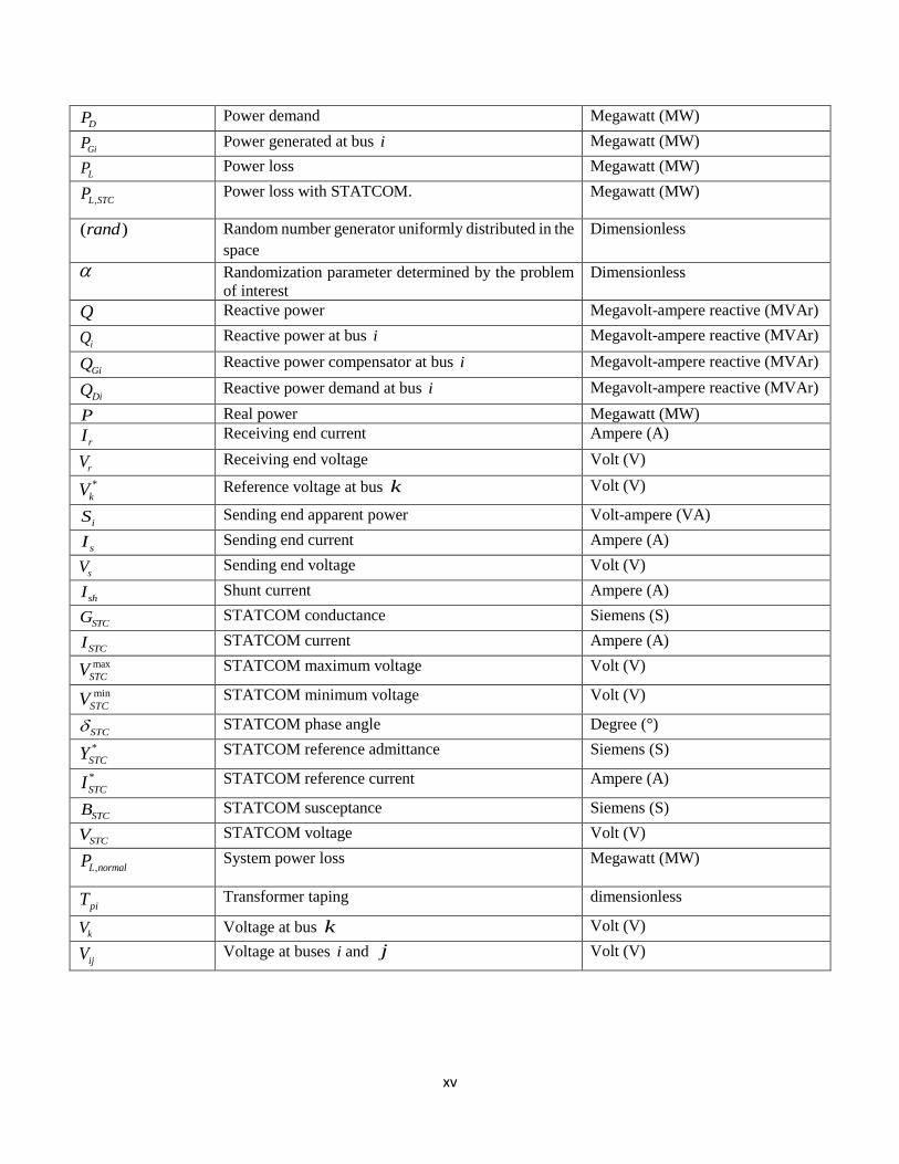
xv
DP Power demand Megawatt (MW)
GiP Power generated at bus i Megawatt (MW)
LP Power loss Megawatt (MW)
,L STCP Power loss with STATCOM. Megawatt (MW)
( )rand Random number generator uniformly distributed in the
space
Dimensionless
Randomization parameter determined by the problem
of interest
Dimensionless
Q Reactive power Megavolt-ampere reactive (MVAr)
iQ Reactive power at bus i Megavolt-ampere reactive (MVAr)
GiQ Reactive power compensator at bus i Megavolt-ampere reactive (MVAr)
DiQ Reactive power demand at bus i Megavolt-ampere reactive (MVAr)
P Real power Megawatt (MW)
rI Receiving end current Ampere (A)
rV Receiving end voltage Volt (V)
*
kV Reference voltage at bus k Volt (V)
iS Sending end apparent power Volt-ampere (VA)
sI Sending end current Ampere (A)
sV Sending end voltage Volt (V)
shI Shunt current Ampere (A)
STCG STATCOM conductance Siemens (S)
STCI STATCOM current Ampere (A)
max
STCV STATCOM maximum voltage Volt (V)
min
STCV STATCOM minimum voltage Volt (V)
STC STATCOM phase angle Degree (°)
*
STCY STATCOM reference admittance Siemens (S)
*
STCI STATCOM reference current Ampere (A)
STCB STATCOM susceptance Siemens (S)
STCV STATCOM voltage Volt (V)
,L normalP System power loss Megawatt (MW)
piT Transformer taping dimensionless
kV Voltage at bus k Volt (V)
ijV Voltage at buses i and j Volt (V)

1
CHAPTER ONE
INTRODUCTION
1.1 Background
Modern power system is an interconnected sub-system which comprises a quite number of generators,
transmission lines, transformers and variety of loads [1 – 3]. The power system is increasing in complexity
due to increase in loop current flows, power demand and line losses [4, 5]. As a result of increase in power
demand, modern day electrical power systems (EPSs) face crucial challenges. The power system is
categorised into three sub-systems viz; generation system, transmission system and distribution system. In
the generation system, electric power is produced, transmitted via the transmission system to the end users.
Transmission system serves as a link between generation system and supply the end users [6 – 9].
1.1.1 Structure of Electrical Power Systems
Electrical power system is defined as a very large network that links power plants i.e. large or small to the
loads, by means of an electric grid. Power system is divided into generation system (power generating
stations), transmission system and distribution system [7]. The significant of a power network is to generate
power in a reliable, secure, and economical manner. The six main power network parts are power generator,
transmission transformer, transmission line, substations, distribution line, and distribution transformer [10].
The power generated in the power system is stepped up before being transferred to various substations via
the transmission line. The power generated is transferred to the distribution transformer where it is being
stepped down to the required value suitable for the end users. Power can be transported through the
transmission and distribution networks. Power systems consist of a meshed transmission lines that cut
across regions which numerous power generators and loads are connected [11, 12].
Transmission systems have the following advantages in power system [7, 11, 12]:
A flattering of the load curve, which makes the use of generation plants more effective.
Power generation economies of scale.
A strong minimization of the reserve margins required at individual generator level, due to outage
of a unit is compensated by all other connected generators in the network, which supply only a
relatively small additional power.
The possibility of minimizing the power cost by moving generation between units by the use of
different prime movers (e.g. coal, gas and oil), depending on the energy source prices [13].

2
The above are the reasons that justify the financial viability of connecting huge power generators by a
transmission and distribution networks so as to securely move the generated power to load, instead of
having a disperse power generating station at every load center [12].
1.1.1.1 Power Generating Station
Fuels are transformed to electrical energy in generating station. The generated voltage which falls between
11 - 25 kV, is stepped up to be transmitted to a long distance. The plants in the generation system can be
categorised into three viz; hydropower plant, thermal power plant, and nuclear power plant. Atomic nuclei
serve as the primary source of energy to generate electrical power in a nuclear power plant; the nuclei are
subjected to nuclear fission to free their energy. The energy released is utilized to produce steam at high
pressure to power a prime mover. In a fossil, fuel powered electrical power generating station, coal, oil, and
gas are fired to produce thermal energy that goes through a steam cycle process to produce electrical energy.
In both cases, a synchronous prime mover, generator, or turbine is utilized to convert mechanical power to
electrical power [7]. When electrical power is generated, the transmission network serve it purpose by
conveying the generated electrical power energy to the loads.
In the last few years, there has been an improvement in the power generation by power system engineers
and researchers due to the fact that the primary source of both modes of power generation discussed above
are limited and they are not environmentally friendly. So, they came up with renewable electrical power
generation which has an unlimited primary resource, with the advantage of being environmentally friendly.
A synchronous prime mover at the renewable power generating station serve two purposes: it connects all
the renewable power plants and it is also used to convert the generated energy to electrical power [14].
1.1.1.2 Power Transmission and Distribution
The transmission network bears the overhead or underground lines that transport the generated energy from
generating station to the distribution substations [10, 15]. The transmitted voltage is operated at above 66
kV and it is standardized at 69, 115, 138, 161, 230, 345, 500, and 765 kV, line voltage. The voltage level
greater than 230 kV is considered as extra-high voltage [7, 16]. The transmission line is terminated in sub-
stations referred to as the primary sub-stations, high voltage sub-stations or receiving sub-stations. In these
sub-stations, the voltage is stepped down to a value suitable for the subsequent flow of power to the end
users. The two main functions of transmission systems are to transport the generated electrical power from
the power generation stations to primary sub-stations and link two or more generating stations.
The distribution system is the power system part, linking the end users in a particular region to the power
plants. The distribution system distributes the power generated to various power users. The main difference

3
between the transmission and distribution systems is that power is transmitted at high voltage and over a
long distance in transmission system compared to distribution systems, which distribute power at low
voltage and over a short distance [11, 17]. This is as a result of the dependency of the capacity of transmitted
power on current and voltage, and losses on the current and length of the line. Therefore, the active and
reactive line losses on transmission network over a long distance are reduced by lowering the current and
raising the magnitude of the voltage resulting in enhancement of power transfer capacity. Increase in
voltage magnitude leads to increase in transmission and transmission component costs. Consequently,
minimization of power loss cost more. This result in an existence of an option of capital expenditure for
equipment to minimize losses for efficient power transfer.
In developing countries, majority of the transmission networks are loaded beyond their capacity than was
planned, when constructed [18]. Availability of electricity is the most powerful vehicle driving economic
development and social changes throughout the world. The supply of electricity involves a large inter-
connection of generators and loads via a transmission systems consisting of transmission lines,
transformers, and other necessary equipment [15].
Unlike in some communication systems where transmission of signals is based on wireless technology,
electricity generated at various generating stations can only get to the consumers at the distribution system
through a transmission network. The transmission system performs the roles of voltage transformation,
power switching, measurement and control. It also provides for redundant system that helps in the smooth
flow of power at a minimum cost with required reliability [19].
Transmission systems are either mesh or longitudinal in nature [20]. Meshed systems are located in high
populated areas where building of generation stations close to the power users, is possible. Longitudinal
networks are located where great quantities of power is required to be transfered over a long distance from
generating stations to end users. Transmission line with low impedance ensures larger flow of power while
the one with high impedance limits the flow of power. Transmission lines are long and have high impedance
which give rise to various operational problems, such as high transmission line losses, voltage limit
violations, loss of system stability and not being able to fully utilize power systems up to their thermal
capacity [10].
Power outages, as a result of disruption of transmission lines, are increasing in the developing nations. This
contributes to the educational dwarfism, economic down turn, technocrats and artisans gross dissatisfaction
due to low business in-flow, consequently; a retrogressive national growth. Almost 1.3 billion people in the
developing nations live with no power supply. With recent global increase in population in rural and urban
areas, the demand for power is increasing and the availability of power systems supplies in developing

4
countries are insufficient for the load. International energy agency (IEA) marked Sub-sahara Africa to have
only 32% electricity supply. A large number of transmission lines are loaded beyond the capacity than was
planned when constructed and there is an urgent need to meet the needs of the population without electricity
[21].
The main objective of analysis of power flow is to obtain the magnitudes of active and reactive load flow
in the transmission network and also, the voltage magnitudes at all the buses of the system for a given
loading condition [2, 3]. Power flow control in power system, is an essential factor affecting the overall
modern system development. As power demand substantially increases, the expansion of generation and
transmission systems have been greatly hindered as a result of environmental restrictions and insufficient
resources. Consequently, majority of the power systems are enomously loaded resulting in the stability of
the system reaching its power transfer-limiting factor [22 – 24]. In contrast to the rapid boom in power
network technologies, transmission networks are loaded to their thermal-limits and simultaneously, stability
limits [18, 25].
Building new power plants and transmission lines as well as using traditional electromechanical devices,
such as synchronous condenser, reactors, capacitor tap-changing transformers, and banks, have been
employed to reduce the transmission systems operational problems [26]. However, long construction time
and regulatory pressure hinder the construction of new transmission networks and generating stations while
low speeds, mechanical wear and tear and high cost of implementation limit the use of traditional devices
[19, 27]. Recently, FACTS devices were introduced in the transmission networks as a result of power
electronic development [28]. FACTS devices control the network condition as fast as possible and this is
exploited to control the system real and reactive power for minimizing losses and voltage magnitude
deviations in transmission networks. These controllers facilitate power flow control, minimize generation
cost, enlarge the power transfer capability, enhance and improve transmission network stability and
security. FACTS devices are electronic based incorporated into the alternating current transmission
networks to increase power transfer capability and enhance controllability [29, 30].
FACTS serves as an attractive means for maximizing the use of the existing power systems, the
enhancement of which has not kept pace with the increase in the capacity of power transmitted through
transmission networks. The power transfer problem is curbed by adding generating and additional
transmission facilities. Interestingly, this problem can be curbed by FACTS controllers without necessarily
altering the system configuration and this is mostly desired by transmission line management companies.
FACTS devices is categorised into series connected, shunt connected and a combination of both [31]. Some
of the shunt connected devices are static synchronous compensator (STATCOM) and static var
compensator (SVC). The series connected comprises static synchronous series compensator (SSSC),

5
thyristor controlled series compensator (TCSC) etc. While for combined shunt and series, unified power
flow controller (UPFC) is a member of this type [32, 33]. STATCOM is use in this research due to it fast
compensating / operating time and less cost of installation. These devices and their mode of operations were
discussed fully in the next chapter.
1.2 Research Motivation and Problem Statement
Transmission systems are constructed in a way to respond to generation and varying load conditions.
Transmission facilities are required to provide equal right to use for power migration to all participants at
all times, ensure reliability and full capability at minimum technical loss and ensure equitable load
allocation to consumers. Power transmission system has been shown to be connected to load centers through
long fragile longitudinal transmission systems, which are subjected to frequent transmission network
collapse due to bad system configuration, high transmission loss, voltage limit violation which does not
allow system reliability [16, 19].
These problems have been solved using electromechanical devices and by power system reinforcement
with construction of extra generating and transmission facilities [34]. Unfortunately, problems associated
with the suggested methods cannot provide effective and immediate solution, hence the use of FACTS
controllers which have been shown to be an alternative to strengthening the voltage profile, load flow and
enhancing the interconnected power system stability [35].
The infinite length of longitudinal network is subjected to high power loss, poor voltage profile and power
flow control. The solution to these problem, as power demanded increases continuously, is to either build
more generation stations (which is expensive) or expand the available transmission infrastructure (which is
not economical) or enhance the existing transmission facilities by incorporating FACTS devices like
STATCOM, SVC and others. FACTS controllers proves as better alternatives for load flow variable control,
voltage profile improvement, minimization of losses, and stability enhancement of the interconnected
power systems. Enhancement of the existing transmission facilities by incorporating FACTS controllers to
increase the power flow, and reduce losses rather than expanding the existing power generation stations is
necessary.
Literature survey confirms that little has been done in applying FACTS controllers to solve the weaknesses
manifested in the longitudinal power system [20]. Also, several researcher have incorporated different types
of FACTS controllers for transmission line control [19], there is no known research that has explored load
flow analysis of the longitudinal system, perform load flow solution by optimally incorporating
STATCOM with meta-heuristic method for power flow control of system variables (active, reactive and
voltage magnitude). Their researches were limited in scope to power flow analysis with Newton-Raphson,

6
Gauss-Seidel, Fast decoupled method without the incorporation of STATCOM. The exchange of power in
a network is facilitated by STATCOM in improving the power supplied to the loads.
1.3 Research Questions
Transmission network is the power system component linking the generated power at the generating
stations to loads. It has been established that in power system, transmission networks account for a larger
percentage of the total losses which increases the total transmission cost and this is undesirable. Therefore,
minimization of losses and voltage magnitude deviations is imperative. Some of the questions that this
research seeks to answer are:
How can the voltage profile of transmission network be improved?
How can the active and reactive losses be minimized on the transmission systems?
What role does STATCOM play in achieving these?
How can STATCOM be optimally sized and placed on the transmission networks?
What methods can be used to optimally size and place STATCOM on transmission networks?
What are the benefits of optimally sizing and placing STATCOM on transmission networks?
1.4 Aim and Objectives
This research aims at investigating the effectiveness of STATCOM device, been optimally sized and placed
with particle swarm optimization (PSO) and firefly (FA) algorithms for power loss reduction and bus
voltage magnitude deviation minimization on a transmission system.
The specific objectives of the study are to:
(a) formulate STATCOM power injection model.
(b) incorporate STATCOM power injection model in (a) into nonlinear algebraic load flow equations,
solved using Newton Raphson power flow algorithm.
(c) simulate the Newton-Raphson load flow algorithm using MATLAB.
(d) determine the performance evaluation of the STATCOM model when optimally installed with
meta-heuristic algorithms in the IEEE 14 bus standard network using voltage profile, active and
reactive power as performance metrics.
1.5 Structure of the Dissertation
Chapter one gives a general introduction of the study, statements of the problem, aim and the objectives.
Chapter two focuses on the literatures review. Chapter three presents the materials and the research
methodology employed in the course of the study. Chapter four presents and discusses the preliminary
results of the load flow analysis of IEEE 14-bus network and when STATCOM was manually placed.

7
Chapter five presents and discusses the simulation results when STATCOM was optimally sized and placed
on IEEE 14 bus system, using PSO algorithm. Chapter six presents and discusses the simulation results
when STATCOM was optimally sized and placed using firefly algorithm (FA). Chapter Seven presents the
conclusion of the dissertation and provides recommendations, based on the research findings, for further
future work.
1.6 Summary
This chapter introduced the subject matters of the research work, and the significance of the study, why it
is expedient to investigate and evaluate the transmission losses and ways to minimize it were discussed.
Moreover, all the methods and the devices used to minimize transmission power loss were briefly discussed.
FACTS devices, which are power electronic based, are usually employed to minimize transmission power
losses as well as to improve the system voltage profile. They are either placed in shunt or series or both on
the transmission network to achieve those objectives. Thus, in respect of that, FACTS devices could be
classified as SVC, STATCOM, TCSC, SSSC, UPFC etc. However, to achieve better results, FACTS device
allocation must be optimally done using any of the meta-heuristic methods. In conclusion, the research
motivation, problem statement, research questions, aim and objectives were stated.

8
CHAPTER TWO
LITERATURE REVIEW
2.1 Introduction
In transmission system networks, reactive power compensators are important in minimizing network
voltage magnitude deviations and losses. The optimal location and size of compensator are very important
to achieve these objectives. Therefore, this chapter discusses some of the devices used for voltage deviation
minimization and power loss reduction in transmission systems. The methods utilized to determine the
optimal location and reactive compensator capacities were discussed while the literatures relevant to this
study were also reviewed.
2.2 Reactive Power Compensator
Reactive power compensators are electrical devices capable of absorbing or injecting reactive powers into
the power network for transfer capability enhancement. They are usually connected at the suitable positions
in the transmission system for voltage magnitude deviation minimization in the power network and also for
minimizing losses. Different types of reactive power compensators are discussed in the following sections.
2.2.1 Capacitor
Capacitor placement in power system network, is an efficient way of improving the power delivery. When
installed in shunt on the transmission line, it is referred to as shunt-compensator. A shunt-compensator
generates the required reactive power into the network. Capacitors connected in shunt, are placed at a bus
to hold the bus voltage levels, injecting required reactive power into network to do so. On the other hand,
a capacitor connected in series is called a series compensator. A series compensator is placed between two
buses in the transmission network to control the line reactive power flow [25, 29].
2.2.2 Flexible Alternating Current Transmission System
FACTS is a power electronics-based system made up of static equipment which is used in transmission of
power. It facilitates the capability and controllability of the network to transfer power [29, 36, 37]. The
Institute of Electronic and Electrical Engineering (IEEE) defined FACTS as equipment that is capable of
controlling one or more transmission network control values to facilitate the capability and controllability
of power transfer. FACTS devices reduces power delivery costs and improves systems reliability. They
enhance the efficiency and quality of transmission system by injecting or absorbing required reactive power
into the transmission network. FACTS devices are of various types among which are static synchronous

9
compensator (STATCOM), static VAR compensator (SVC), unified power flow controller (UPFC),
thyristor-controlled series capacitor (TCSC) and interline power flow controller (IPFC) [7, 10, 25].
2.3 Application of Power Electronics in Power System
Power electronics is the application of solid-state electronics for the control and conversion of electric
power [38]. It is impossible to give a lists of power electronics applications in today’s world; it has entered
nearly all the fields where electrical energy is in use [39]. The ease of manufacturing has also led to
availability of these devices in a vast range of ratings and has gradually appeared in power system. Power
electronics devices used in power system are: high voltage direct current (HVDC) links and FACTS
devices. The HVDC links is another way of transmitting electrical power, while FACTS controllers are
applied for reactive power compensation and power system improvement. These devices used in the
distribution system are employed to improve the system power quality and are usually called custom power
devices, while the devices on the transmission system are optimized to reduce losses by balancing the
reactive power [11, 40]. Figure 2-1 shows a brief diaspora of power electronics.
Figure 2-1: Diaspora of power electronics [25].
They are widely applied in power system, and promotes development of power system towards a more
intelligent and sustainable direction. The power electronic converter processed 60% of the final electric
energy used in developed country at least one time according to the data. Which means, power electronics
contributes greatly in power system to the power generation, power transmission, power system harmonics
control, power supply stability, etc. [19, 29].
10
2.3.1 Distribution Level
As power electronics controllers are utilized to improve stability in transmission networks and control
power flow, likewise are the custom power devices used to enhance quality of power in distribution system.
Problems with harmonics, damages related to transient over-voltages, or tripping of equipment as a result
of voltage dips has led to the use of adjustable and dynamic devices to curb these problems [7]. Unlike
FACTS devices, custom power devices are also placed in different ways: series-connection, shunt-
connection, combine series-shunt connection [13]. Type of customs devices used in the distribution system
are discuss below:
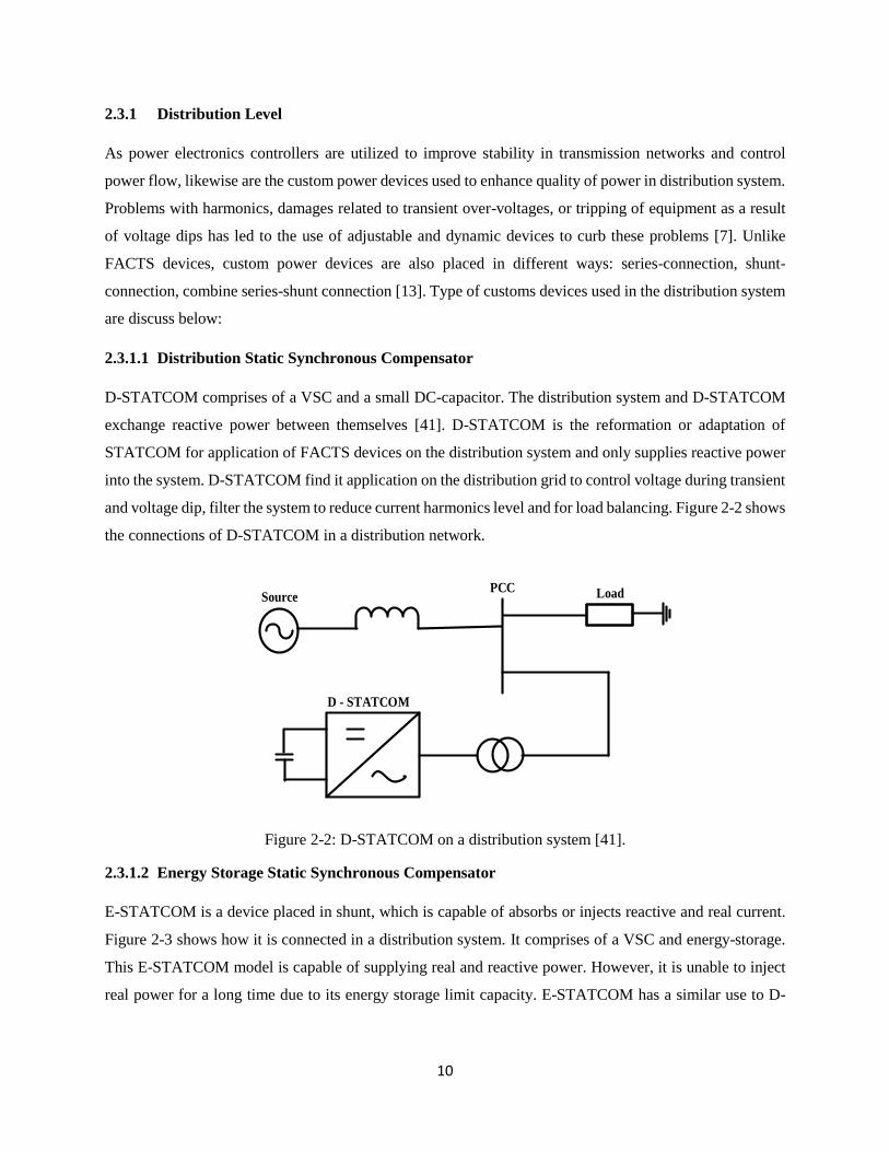
2.3.1.1 Distribution Static Synchronous Compensator
D-STATCOM comprises of a VSC and a small DC-capacitor. The distribution system and D-STATCOM
exchange reactive power between themselves [41]. D-STATCOM is the reformation or adaptation of
STATCOM for application of FACTS devices on the distribution system and only supplies reactive power
into the system. D-STATCOM find it application on the distribution grid to control voltage during transient
and voltage dip, filter the system to reduce current harmonics level and for load balancing. Figure 2-2 shows
the connections of D-STATCOM in a distribution network.
Source LoadPCC
D - STATCOM
Figure 2-2: D-STATCOM on a distribution system [41].
2.3.1.2 Energy Storage Static Synchronous Compensator
E-STATCOM is a device placed in shunt, which is capable of absorbs or injects reactive and real current.
Figure 2-3 shows how it is connected in a distribution system. It comprises of a VSC and energy-storage.
This E-STATCOM model is capable of supplying real and reactive power. However, it is unable to inject
real power for a long time due to its energy storage limit capacity. E-STATCOM has a similar use to D-

11
STATCOM, with the exception of its energy storage capacity which exchanges active power with the
system [11].
Figure 2-3: E-STATCOM on a distribution system [12].
2.3.1.3 Dynamic Voltage Restorer
Dynamic voltage restorers (DVR) are series devices comprising of a VSC which produces injected a.c.
voltages for voltage sag improvement via injection transformers [41]. The major advantage of the use of
the DVR to mitigate the voltage drop is its dynamic performance, which is not dependent on the source
impedance. Likewise, it can be deployed to compensate for unbalanced voltage and filter voltage
harmonics. The only draw back of DVR is the increase in cost as a result of the requirement of an advanced
protection system if a short circuit fault occurs [12]. Figure 2-4 presents the configuration of a DVR in a
distribution network.
Figure 2-4: DVR connected to a distribution system [41]

12
2.3.1.4 Static Transfer Switch
Static transfer switches (STS) is another means of protecting a sensitive load from voltage dip. Either the
primary or secondary feeder can feed a load with static transfer switch. The thyristor switches the device
from the primary feeder to the secondary feeder in cases of voltage dip. The STS only protects equipment
in the distribution system; if there is a voltage dip in the transmission system, both feeders of this device
will be affected [11]. Figure 2-5 shows the connection in a distribution network.
Figure 2-5: STS connected on a distribution system [12].
2.3.1.5 Uninterrupted Power Supplies
Uninterrupted power supplies (UPS) come in various structures but the common denominator of all UPS is
that its energy storage can supply active power. The size of the UPS energy storage determines its capacity
to mitigate power interruption, voltage drop, and other power quality problems. UPS of about 5000 kVA
can be deployed for low power equipment that is sensitive, such as computers and servers [11]. Its
connection with distribution system is shown in Figure 2-6.
Figure 2-6: UPS connected on a distribution system [12].

13
2.3.2 Transmission Level
HVDC is the first power electronics technology to be used in power network, which began with the use of
mercury ionic valves [11]. The HVDC finds more use in long distance overhead and underground
transmission systems, as an alternative means to transport power. It is also used to connect AC systems of
different frequencies [29]. The transmission capacity of transmission networks is increased to their thermal
capacity limit by using FACTS devices,. FACTS facilitates control of voltage when there is contingencies
and stop the flow of loop currents which is responsible for unnecessary loading of transmission network
facilities [42].
Also, FACTS devices are applied to compensate and improve on an existing AC transmission system where
there is a need to enhance the capacity of the system on power delivery. It has been proven that there is a
significant increasing demand for electrical power leading to the complexities of the transmission system
[21]. Considering the time and cost to build a new transmission line, FACTS comes in as a viable and
attractive alternative [19, 24]. FACTS devices could be placed in series, parallel, or combined mode.
2.4 Overview of Flexible Alternating Current Transmission Systems Devices
FACTS controllers are power electronic controller circuit configuration which are very effective in
regulating power flow on a.c. transmission lines. FACTS devices are an evolving technology to help electric
utility companies. Load flow in the transmission network and bus voltage profile are easily controlled with
FACTS technology applications. Iincrease in the useable transmission system power capacity and flow
control over the transmission routes is the main goal of FACTS controllers [25]. FACTS devices are divided
into two generations based on the technological features viz; the first and the second generations [26]. In
the first generation, FACTS devices use thyristor as the power semiconductor switching device in
conjuction with a large reactor or capacitor banks for absorbing or injecting reactive power from or into the
transmission network. In second generation, FACTS devices use GTO or IGBT as the power semiconductor
switching device in conjuction with small capacitors. The ability to interchange and generate real and
reactive power is the main difference between the two generations of the FACTS devices [27].
The most advanced type of the controller among the FACTS controllers, are those which use VSC as
synchronous sources. STATCOM controllers are of the VSC type, which are connected in shunt, so also
are the SSSC controllers which are series connected and UPFC, which is a series/shunt type controller. Of
all the VSC the most widely used is the STATCOM [28]. Figure 2-7 shows the classification of member
of each generation.

14
Figure 2-7: Overview of member FACTS generation [43].
FACTS devices are applied as follows [43]:
(i) increase of transmission capability
(ii) power flow control
(iii) power conditioning.
(iv) compensation of reactive power,
(v) voltage control
(vi) improvement of network stability
(vii) improvement of power quality
2.5 Basic Types of Flexible Alternating Current Transmission System
FACTS controllers are classified to four categories depending on how their connections in the transmission
system bus. Electronics-based FACTS devices have replaced many mechanically controlled reactive power
compensators. Furthermore, they play a role in the control and operation of transmission networks [7, 10,
29, 44 – 46].
Shunt controllers
Series controllers

15
Combine series-series controllers
Combine series-shunt controllers
2.5.1 Series Controllers
The series controller is either a variable impedance for examples, a reactor, thyristor switched, capacitor or
a power-electronics based variable voltage source that supplies series voltage. Figure 2-8 depicts the
connections of this controller on transmission network. The current flowing through the variable impedance
is multiplied by the impedance, which inject series voltage on the transmission network. In this case, the
device requires a energy source connected externally to it. This device either injects or absorbs reactive
power when the voltage is more or less than 900 out of phase with the line current.
Figure 2-8: Basic series controller [29].
2.5.2 Shunt Controllers
The shunt device can either have a variable current and impedance or voltage source in addition to a reactor,
or capacitor, placed in shunt in the transimission network to produce reactive power into the line as depicted
in Figure 2-9. The shunt device either injects or absorbs reactive power when the current injected is more
or less than 900 and is out of phase with respect to the voltage.
Figure 2-9: Basic shunt FACTS controller [29].

16
2.5.3 Combined Series Series Controllers
Combined series series controller is a combination of two or more separate series devices on a transmission
network, which are controlled in a coordinated manner. These controllers possess the capacity to balance
the flow of power in the network through the DC link whereby the transmission network is maximally
utilized. For real power transfer, the DC-terminal of all the device is connected, therefore it is called UPFC.
Figure 2-10 shows this controller type.
Figure 2-10: Basic series series FACTS controller [29].
2.5.4 Combined Series Shunt Controllers
The combined series-shunt controllers utilize both series and shunt devices on a transmission network,
controlled in coordinated manner. The combined series- shunt devices supply series line voltage with the
series part of the device and supply current to the network with the shunt part as depicted in Figure 2-11.
Figure 2-11: Basic series-shunt FACTS controller [29].

17
2.6 Shunt Devices and Operational Principle
The basic operational principle of shunt device is the injection of the reactive power which the load required.
shI could be controlled by varying the shunt controller impedance for adjusting the current I in the line.
The transmission line voltage-drop is related to current I in the line. When the sending end voltage sV
assumes a constant magnitude, the shunt devices is utilize for adjusting the receiving end-voltage value
rV as depicted by Figure 2-12 [47].
Figure 2-12: Operating principle of shunt controller [47].
This relationship shI and rV is expressed as in Equation (2-1):
𝑽𝒓 = 𝑽𝒔 − 𝑰𝒁
𝑽𝒓 = 𝑽𝒔 − (𝑰𝒓 − 𝑰𝒔𝒉)𝒁 (2-1)
The current shI compensated the load current rI partly, which reduce the line current I when the line is
heavily loaded which results in low voltage-drop. Through varying the impedance, the voltage magnitude
is controlled accordingly by the shunt device. Shunt devices are distinguished into three types viz; SVC
devices, switched shunt-capacitor and inductor devices and STATCOM. The switched shunt-capacitor and
inductor controller has only two status (high and low). Its simplicity in mode of operation and principles
are too simple, which makes it not to be relatively used. Its configuration is shown in Figure 2-13. The
remaining two shunt devices are discussed below.

18
Figure 2-13: Configuration of switched-shunt capacitor and inductor [47]: (a) capacitor; (b) inductor.
2.6.1 Static VAR Compensator
This device provides fast-acting reactive power on high-voltage electricity transmission networks. The term
“static” signifies that the device has no moving components. Basically, SVC divided into two type [10, 29,
46]:
Fixed Capacitor Thyristor Controlled Reactor (FC-TCR)
Thyristor Switched Capacitor Thyristor Controlled Reactor (TSC-TCR).
TSC-TCR is frequently used than FC-TCR due to its flexibility and that it requires reactor of smaller rating
which produce smaller harmonics [31]. Figure 2-14 depicts a typical SVC connection. The TSC-TCR SVC
type comprises a series capacitor or an inductor with inverse-parallel thyristor. Inverse-parallel thyristors
is used in TSC to quickly switch the capacitor on and off instead of mechanical connectors. The inrush
currents are limited by a small series inductor when severe transience happens, especially during the process
when the capacitor begin to charge initially.

19
Figure 2-14: Typical configuration of SVC [47].
Figure 2-15: Terminal V-I characteristics of SVC [43].
Firing angle control is employed in TCR to fire the thyristors to change the current which results in control
of the shunt TCR reactance. The firing angle is delayed by 900 delay to 1800 delay to ensure uninterrupted
conduction. SVC can function as a controllable capacitor or inductor, to inject or consume required reactive
power to the transmission bus. When it is effectively located, it gives optimum performance on transmission
line. The main disadvantages of SVC are that firstly, in terms of supplying required reactive power, it is
less effective for low bus voltage. Secondly, SVC produces current with great number of harmonics, thereby
requiring a low cutoff frequency filter to reduce these harmonics in the current [47].

20
2.6.2 Static Synchronous Compensator
STATCOM is a power electronics based VSC which could inject or absorb reactive power from the
transmission system. It comprises a DC capacitor, a VSC and a coupling transformer [8]. Leading or lagging
quadrature a.c. current can be injected by the STATCOM into the grid voltage, emulating a capacitive or
an inductive impedance at where it is connected [48 – 50].
Figure 2-16 shows the one-line diagram of STATCOM controller in which a magnetic coupling is connects
a transmission network bus to a VSC. By changing the magnitude of the converter 3-phase output voltage,
E1, the reactive power exchange between the a.c. network and the converter can be adjusted. Increase in
output voltage magnitude above the transmission network bus voltage, V, will result in flow of current
through the converter reactance to the a.c. network. This makes the converter to injects reactive power into
the a.c. system. Decrease in the output voltage magnitude below the transmission network bus voltage, will
result in flow of current from the a.c. network to the converter and thus consuming reactive power from the
network [51]. The reactive power exchange is nil when the a.c. network voltage equals the converter output
voltage. Furthermore, STATCOM performs the following [46, 52];
(i) It occupies a small footprint, i.e. compact electronic converters replace passive banks of circuit
elements;
(ii) It provides modularity, factory-built equipment, thereby minimizing site work and commissioning
time;
(iii) It utilizes encapsulated electronic converters, thereby reducing its environmental impact.
Figure 2-16: STATCOM configuration [7].

21
Figure 2-17: Terminal V-I characteristics of STATCOM [10].
Incorporation of STATCOM into load flow studies needs adequate STATCOM modelling in the load flow
algorithms. STATCOM have two well tested models viz; the current injection model (CIM) and the power
injection model (PIM). In CIM, a current source is placed in parallel whereas in PIM, a voltage source
behind an equivalent reactance, is connected in paralle on the transmission network for adjusting the
voltage. Steady state STATCOM power injection model reliability is very high when it is incorporated into
the transmission network and is well documented [30, 43, 53, 54].
2.7 Advantages of STATCOM Over SVC
The major purpose of shunt connected FACTS devices on the system (transmission network) is to provide
adequate reactive power compensation that is needed for effective operation of the system. Both SVC and
STATCOM are important or elegant member of first and second generations shunt connected FACTS
devices. Each of them plays a vital role in solving or mitigating problems in transmission network,
especially in voltage magnitude minimization, loss minimization, system stability and security. To stabilize
the voltage level in a transmission network, compensation of reactive power is required, since imbalance
reactive power can cause breakdown of the power system. STATCOM operation advantage can be applied
to minimize and compensate for such reactive power imbalances. As a result of fast-switching times of
IGBTs (self-commutating power semiconductor) of the VSC. STATCOM responds faster than SVC and its
harmonic emissions are lower. STATCOM requires less space because of its elimination of large passive
components; it requires less maintenance without the problem of loss of synchronism [12, 38, 52].

22
Another merit of STATCOM is that compensating current is independent of the system bus voltage
magnitude at the connection point, unlike SVC that experience lower compensating current as the voltage
dips [39]. By comparing the cost of SVC to that of STATCOM, it becomes obvious that it is relatively
cheap to install and maintain and when connected in transmission systems, it provides the voltage needed
for stability, but it is poor in terms of voltage regulation - voltage regulated by the SVC maybe greater than
1.05 p.u. A VSC PWM based STATCOM was investigated in this dissertation to mitigate power losses in
a transmission network. Tables 2-1 and 2-2, below shows the different basic operational principles and cost
of both shunt FACTS devices respectively.
Table 2-1: Different basic operational principles of SVC and STATCOM [55].
SVC (Thyristor based shunt compensator) STATCOM (VSC based shunt compensator)
SVC operates as a shunt connected reactive
admittance control
STATCOM functions as a shunt connected
synchronous voltage source
SVC does not provide active power compensation STATCOM provide active power and reactive
compensation
Table 2-2: Comparison of cost of shunt devices [55].
SHUNT DEVICES COST (US $)
Shunt capacitor 8 / kVar
SVC 40 / kVar
STATCOM 50 / kVar
Table 2-1, shows the differences that account for STATCOM’s superiority over SVC, for greater
application flexibility and better performance. STATCOM increases flexibility and boosts power system
performance, provides instant detection of voltage disturbance, and rapidly compensates by injecting
leading or lagging reactive power. STATCOM provide fast recover time for utilities, from system voltage
collapse events and eliminates stability-related power transfer limitations, with advanced controls. More
importantly, it is a cost effectives solution with minimal footprint. STATCOM performed better than SVC
when incorporated on the transmission network to mitigate power system problems.

23
2.8 Optimal Power Flow
Optimal power flow (OPF) is an essential tool for network operators in operating and planning stages. In
order to optimize an objective function in an OPF, there is a need to find the values of all the control
variables. The problem must be defined with objectives given at the onset, being stated clearly. Objective
function can take different forms such as transmission losses, reactive source allocation and fuel cost [43,
56, 57].
The total production cost of scheduled generating units is the objective function to be minimized. It is
mostly utilized because current economic dispatch practice is reflected and importantly cost related aspect
is always ranked high among operational requirements in Power Systems. The aim of OPF is to minimize
an objective, with the system load flow equations and operating limits of the equipment being the
constraints that it is subjected to. The optimum solution is obtained by adjusting the controls to optimize an
objective function subject to security requirements and specified operating [7, 58].
2.9 Solution Methodologies for Optimal Power Flow
A quite number of algorithms for solving optimal power flow have been proposed and applied on power
network. Two major categories are recognised viz; the intelligent and conventional methods. In
conventional method, the solution approaches have some disadvantages which make artificial intelligent
algorithms to be used [43]. The broad views of the above itemized methods are subsequently presented.
2.9.1 The Conventional Solution Methodologies
The conventional or classical approaches are otherwise known as deterministic approach optimization
methods. Examples are Gradient Method (GM), Dynamic Programming (DP), Linear Programming (LP),
Quadratic Programming (QP), Newton Methods (NM), Lagrangian Relaxation Algorithm (LRA), Non-
Linear Programming (NLP), Interior Point (IP) Methods and Hessian Methods. Many of these conventional
techniques are employed most especially when the search space is non-linear [30].
Despite the scholarly advancements that have been made in classical approaches, yet classical approach
presents some limitations in its implementation. The identified limitations among others include [10]:
(i) Poor convergence.
(ii) The solution is highly computationally expensive.
(iii) Finding a single optimized solution and the treatments of operational constraints are somehow
tedious.
Most deterministic optimization methods are viewed as local search methods because they are known for
producing the same set of solutions if the algorithm starts under the same initial conditions [47].

24
2.9.2 Intelligent Solution Methodologies
Intelligent methods also known metaheuristic optimization methods which are based on artificial
intelligence. Examples are Cuckoo Search Algorithm (CSA), Bacterial Foraging (BF), Particle-Swarm
Optimization (PSO), Artificial Bee Colony (ABC), Pattern Search (PS), Evolution Programming (EP),
Firefly Algorithm (FA), Differential Evolution (DE), Harmony Search (HS), , Hopfield Neural Network
(HNN), Gravitational Search Algorithm (GSA), Genetic Algorithm (GA) and Tabu Search (TS)among
others. Researchers had shown that these algorithms are endowed with [59 – 61];
(i) Faster convergence rate.
(ii) Ability to attain global solution within shortest time possible.
(iii) Efficient capabilities for handling complex system.
A comparison of various intelligent methods for solving OPF problems showing their strengths and
weaknesses is presented in Table 2-3.
This research aims to determine optimal placement and sizing of STATCOM in minimizing power losses
and voltage magnitude deviations on the transmission lines. STATCOM is a VSC based controller that
offers support to power system by providing reactive power compensation and rapid voltage control in
power system. STATCOM increases the transmission line capacity, enhances the voltage profile, angle
stability and dampens the oscillation mode of the system. In recent years, STATCOM attracts the mind of
power researchers and operators for supporting the system by supplying the required reactive power and
for voltage profile improvement on the transmission networks. The placement of STATCOM is an
optimization problem which requires reducing the system loss and voltage magnitude deviation and
satisfying system constraints.
Table 2-3: Comparison of Meta-Heuristic Optimization Algorithms [37, 59, 60, 62 – 66].
Meta-heuristic Optimization
Algorithm
Merits Demerits
Particle Swarm Optimization
(PSO)
The concept is simple and easy
to implement.
Parameter control is robust and
requires lesser memory.
Application to non-linear,
discontinuous problem is easy.
When handling heavily constraint
problems, It is trapped in local optima
as a result of limited local/global
searching capabilities.
It can be easily updated without
solutions quality consideration.

25
Ant Colony Optimization Applicable to a broad range of
optimization problems.
Since ants move simultaneously
and independently without
supervision, it can be used in
dynamic parallel applications.
Positive feedback favoring most
taken path leads to discovering
good solution rapidly.
It avoids premature
convergence when computation
is distributed
Theoretical analysis is difficult so
research is experimental instead of
theorectical.
Although convergence is guaranteed,
but it takes uncertain time to achieve
this.
Applied only to discrete-problems
Artificial Bee Colony Requires few values.
It is used globally.
High flexibility
High computational time
BAT Algorithm
High flexibility and simple to
implement.
Requires few control
parameters.
Initial convergence is fast.
Application to non-linear
discontinuous functions.
It could lead to stagnation after initial
stage, if it is rapidly switched from
exploration to exploitation stage.
Grey Wolf Optimization
Easy implementation as a result
of its structure.
Converges rapidly.
Requires few number of
parameter.
Local optima are avoided.
The algorithm is still under research
and development.

26
Meta-heuristic Optimization
Algorithm
Merits Demerits
Bacterial Foraging
Optimization Algorithm
Adapt automatically.
It converges globally thus avoiding
premature convergence.
Computation is very fast.
Less memory requirement.
Wide application to nonlinear
functions and handling of more
objective functions.
Swarming effect is unsatisfactory for
ELD problem as a result of its biased
random walk.
Shuffled Frog Leaping
Algorithm
It is accurate, robust and efficient.
It combines the profits of the local
search tool of PSO and mixing
information idea from parallel local
searches to toward a global
solution.
Gets trapped in local optima.
The convergence to proper target is
very late.
Firefly Algorithm
It only includes self-improving
process with the current space but
also include.
It improves its own space
Computation to reach optima is
rapid.
Rate of convergence is high and
much easier.
It is a hybridized version of APSO,
HS, SA and DE.
Automatic division of the whole
population in subgroup.
Has inherent ability to deal with
multi-modal optimization.
May be trapped into local optima if
the values are not well set.
Parameters are fixed.
No memory of previous iterations
better solutions.

27
It has high periodicity and diversity
in the solution.
Genetic Algorithm
It can easily handle the integer or
discrete variables since it works
with coding of parameter set.
It uses only objective function
information, not derivatives or
other auxiliary knowledge.
It is time consuming.
It has many control parameters.
It is difficult to formally specify
convergence criteria being a stochastic
algorithm.
Various nature inspired meta-heuristic algorithms as mentioned in Table 2-3, are used to solve the problem
of STATCOM placement. This dissertation proposes the use of PSO and FA for STATCOM placement to
reduce power losses and voltage magnitude deviations. The choice of FA and PSO are driven by their
computational efficiency, quick convergence, control parameters lustiness, easy deployment and simple
concepts. The algorithms identify the parameters of the STATCOM and the most suitable STATCOM
location. Simulations were carried out on standard IEEE 14-bus network using Matlab computer program.
2.10 Review on Previous Works
Several researches have been conducted in the area of optimal determination of the most suitable reactive
power compensators location in a transmission network for voltage magnitude and power loss reduction.
The two most popular solution methods which are reported in literature are the sensitivity techniques and
mathematical optimization. The mathematical optimization approach consists of both analytic and heuristic
techniques. The sensitivity technique predicts buses/areas where compensators could best located by using
certain characteristic of the network. This section of the dissertation reviews some of the works conducted
in this area.
ANN based STATCOM and conventional PI based STATCOM model of 132 kV transmission network
were simulated with comparison by authors in [67]. Result after simulation showed that the power factor
was restored into unity by STATCOM which enhanced the transmission network transfer capability by
either injecting or consuming required value of reactive power. STATCOM with ANN controller gave a
rapid response time when compared with PI Controller. In addition, ANN controlled STATCOM enhanced
system stability and dynamic response of the network better than conventional PI based STATCOM.
A control strategy was proposed by authors in [68] for PSO based STATCOM, adjusting the parameter of
PI control loop online adaptively. A small scale STATCOM controller incorporated grid was developed

28
and simulated using a model based on electromagnetic transient. STATCOM with a control utilizing a
conventional double closed-loop and PSO based intelligent control system were also designed, analyzed
and the results compared. The grid voltage was significantly improved by PSO as revealed by the result
showed the validity of PSO based STATCOM control strategy.
Determination of the appropriate STATCOM location and parameter setting using the Moth Flame
Optimization (MFO) algorithm was proposed by authors in [32]. Incorporation of STATCOM in
transmission network was done to reduce voltage deviations, enhance system stability and minimize loss.
The algorithm was validated on IEEE 30-bus system. Comparison of the optimization algorithm which
include a simplified STATCOM model was made with the conventional PSO. The OPF problems
formulated to verify the device effectiveness, was solved with and without STATCOM incorporation. The
simulation results revealed that the developed algorithm was superior in optimal STATCOM location
determination.
System voltage deviation was reduced by authors in [69], using STATCOM controller allocation. The
fitness value which comprises total voltage deviation and real power loss was reduced by placement of
UPFC controller. This results in decrement in the total loading of the network line. Differential Evolution
(DE) was chosen for optimally sizing and placing of FACTS controllers. Simulation was performed on
IEEE 30-bus network. The results further showed reduction in total deviation of the voltage with increased
in load by 90%. Differential Evolution algorithm also reduced congestion significantly after placement of
UPFC.
Hybrid STATCOM comprising of active inverter part and thyristor-controlled LC part was used by authors
in [70] to overcome the shortcoming of reactive power compensation. Simulation of Hybrid STATCOM
was completed using the MATLAB/Simulink. From the simulation, the performance of the hybrid
STATCOM was determined. Testing of the Hybrid STATCOM was performed during unbalanced current
conditions and voltage dip. The hybrid STATCOM was found to have higher compensation capability than
conventional STATCOM.
Simulation of STATCOM and SVC was carried out by the authors in ref. [31], using
MATLAB/SIMULINK and a comparative analysis was done. The results showed STATCOM effectively
stabilized the voltage. When the breaker closes, the device supplies reactive power to the system. As soon
as the breaker closes, the voltage profile suffers a change but is recovered soon with the application of
STATCOM that injects reactive power into the network. The regulated rms voltage showed a reasonably
smooth profile in spite of sudden load changes, where the transient overshoots are almost nonexistent. The
transients were kept at a very small values with respect to the reference voltage.

29
The STATCOM principle structures and its midpoint voltage regulation impact was explained by authors
in [39]. The STATCOM performance with that of conventional SVC under different fault conditions were
compared. MATLAB/SIMULINK software was simulated used as simulation tool and the results revealed
that STATCOM is more effective in regulation of midpoint voltage on the network.
Reduction of transmission power loss was performed by authors in [71] using hysteresis band current
(HBC) controller-based STATCOM. The authors designed and analyzed a STATCOM controller for linear
and non-linear loads. Simulation was performed by the use of MATLAB software and the results showed
mitigation in losses in the system.
A control strategy for limiting fault-current by the use of dual STATCOM was used by authors in [72], to
reduce power oscillations and minimize the voltage- dip as a result of a serious symmetrical fault. This was
achieved by divertion of the fault current to the capacitor using the dual-STATCOM controller. They
observed that it was best suitable to maintain stability with uninterrupted power supply, effective power
transfer capability and rapid reactive power support and to reduce inter-area oscillations. The SG and DFIG
effectiveness as a result of symmetrical short-circuit fault in the network was investigated. The author
observed that voltage magnitude deviations were mitigated and surge-current was minimized in both areas.
The power oscillations were reduced, and SG q-axis voltage was regulated to nearly the same magnitude
before, during and after the fault. From the results, dual STATCOM proved to be a better device than single
STATCOM.
The practical and theoretical applications of STATCOM controller for controlling voltage and optimizing
active power losses was described by the authors in [73]. They used STATCOM controller to vary the bus
voltage and to reduce active power losses. PSO application revealed the potentials of this technique in
transmission system to enhance their operation.
A micro grid system which could deliver power to dynamic loads was investigated in [74]. The system
comprises a photovoltaic and a constant power micro-hydro system, connected via a fuzzy controlled
STATCOM controller together with an energy-storage system. The STATCOM injected the required
reactive power to the network to regulate the voltage and frequency and to also ensure good power quality
in the network. The performance of the hybrid microgrid system was evaluated using various types of loads
among which are nonlinear load, dynamic load, and linear load. MATALB/Simulink software was used for
simulation. The results revealed that device capability in stabilizing the network parameters various load
conditions.
A differential-evolution and chemical-reaction optimization hybrid chemical-reaction optimization
approach was proposed by author in [75], to determine the appropriate location and STATCOM parameter

30
settings to ensure optimal performance of network. Optimal STATCOM allocation was done by the use of
hybrid chemical reaction optimization, for reducing the network loss and improve the voltage profile in a
transmission network. The algorithm was successfully applied to IEEE 30-bus network. The HCRO
technique is superior to other discussed algorithms discussed by the authors.
STATCOM was used by the authors in [76], to connect hybrid-power network to the grid. In their work,
they use wind and solar power source for the hybrid network. The sources were not connected directly to
grid because the power output of these two sources are not constant,. By the use of STATCOM, the hybrid
power network output of was regulated. Although, STATCOM input varied continuously but its output was
regulated with the aid of Icos current component. MATLAB software was used to simulate system to
obtain good waveforms.
A coordinating scheme for ULTC and STATCOM was presented by the authors in [77]. In their work, some
manipulations were made in the STATCOM control system to coordinate ULTC and STATCOM. On the
basis of the proposed scheme, STATCOM capacity was minimized and hence some compensating margins
provided for control purposes in emergency situations. The major merit of the technique is the modification
of STATCOM control system to some extent but and the control of ULTC is unchanged.
Consideration of optimal allocation method which focuses on return of investment index of high cost
STATCOM and involves huge economic loss of the voltage sags was proposed by author in [78]. Firstly,
voltage-sag-severity index and voltage-sag-economic loss index based on quality engineering theory, were
presented. Secondly, the author puts forward STATCOM return on investment index to assess the economic
benefit of different installation capacity by comparing the voltage sag economic losses before and after the
installation of STATCOM controller. Finally, an optimal reactive compensation allocation technique which
is based on above economic benefit evaluation indexes was presented. The method presented ensures safe
reliability of network and achievement of the optimal economic benefit.
Active and reactive power loss reduction in network was proposed by authors in [79] using STATCOM
based on hysteresis band current (HBC) controller. The active and reactive power losses in the transmission
system was reduced by compensating load reactive power. The STATCOM controller design and analysis
for nonlinear and linear loads were done. The analysis was performed for a 3ϕ induction motor, a 3ϕ battery
charger and a 3ϕ transformer. The results showed that losses were greatly minimized that the STATCOM
based hysteresis band-current controller is more effective than the conventional controllers in minimizing
losses.
The topology and performance of T 3-level inverter based on the principle and topology of three level
traditional NPC inverter was analyzed by authors in [80]. They proved T three level inverter superiority

31
and also built T 3-level inverter-based D-STATCOM model. By the use of hysteresis control method, D-
STATCOM compensation effect under three modes of dynamic switching, constant reactive compensation
and sudden load variation was analyzed by the authors. The working characteristics of T three level-based
D-STATCOM inverter were verified. Results showed fast-dynamic response of hysteresis control T type
three level STATCOM. This new type of STATCOM supplied the reactive power demanded.
Authors in [81], dealt with the use of STATCOM PV farm inverter to stabilize the voltage where it is
connected which improves the stability. The solar farm normally produces real power during the day but
remains inactive at night time. The proposed solar system working as a STATCOM is known as PV
STATCOM. This scheme uses total capacity of inverter during night time and that remaining after real
power production during the day for carrying out various STATCOM operations. The entire system
modelling and analysis were done on a single machine system having midpoint connected PV-STATCOM
using Matlab software. This PV-STATCOM in the field of PV-solar gives rise to new opportunities to earn
profit in the nighttime and daytime along with the sale of active power during the day
The oscillations system operation in inter-area mode was investigated and analyzed by authors in [82]. They
used Kundur model which is a power system with two area with implementation of each of selected FACTS
devices which were implemented to a specific place in the network to noté the dynamic performances of
STATCOM, TCSC and SSSC on inter-area. The simulation results showed that power oscillation damping
of the specific power network and contingency conditions was enhanced with adequate FACTS controller
sitting and parameter settings.
2.11 Summary
An overview of the most salient characteristics of the power electronic equipment used in regulation of
voltage, active and reactive load flow control, and power quality enhancement has been presented. The
applications and performance of TCR, TCSC, SVC, UPFC, SSSC, and STATCOM among other FACTS
devices were discussed. It was observed that STATCOM has some advantages in terms of reactive power
injection, response time, and cost of implementation as earlier presented. Therefore, STATCOM forms the
major FACTS device used in this research work and has been extensively discussed and properly reviewed.
Besides, in all the reviewed and mostly the available articles, there has not been applications of particle
swarm optimization and firefly algorithms concurrently, for optimization of STATCOM device for the
purpose of power loss reduction and bus voltage profile deviation minimization, hence this work. The
achievement of the above mention objectives via implementation of an optimally placed STATCOM
device, through independent and comparative optimization algorithms, involving FA and PSO formed the
vantage of inference deduced from the review of the literature in this chapter.

32
CHAPTER THREE
RESEARCH METHODOLOGY
3.1 Research Approach
This research is based on the basic principles and theories of constrained optimization problems. The
problems to be minimized are the power losses, while bus voltage magnitude minimization is also
considered as part of objectives. These are to be achieved with optimal STATCOM controller placement
and sizing by the use of PSO and FA. A single-objective solution method was used to find the optimum
size and most suitable location of STATCOM controller that will reduce the losses of the network and
minimize voltage magnitude deviation. Mathematical modeling of STATCOM power injection was
formulated appropriately for incorporation into the standard IEEE 14-bus. Newton-Raphson (N-R) power
flow method was used, because of its fast quadratic convergence. PSO and FA were chosen as optimization
methods for allocation of STATCOM controller as they only require minimum manipulation to solve
optimization problems and their ability to attain global optimum solution.
STATCOM data were obtained from published open access literatures on the concept. The STATCOM
power injection model (PIM) was included in the Newton Raphson algorithm and simulations were carried
out using Matlab programme. The modified N-R was then implemented on a standard IEEE 14-bus. PSO
and FA were evaluated with real and reactive power loss minimization and voltage magnitude minimization
as performance metrics.
3.2 Problem Formulation
The STATCOM power injection model was incorporated in Newton-Raphson (N-R) for load flow analysis
and treated as an optimization problem and formulated as a single-objective optimization problem to reduce
the total active and reactive power losses and voltage magnitude deviation of transmission network subject
to series of equations that characterize the flow of power in the transmission network and STATCOM
controller. The objective is to find the appropriate STATCOM controller location and size to reduce the
active and reactive losses and consequently improves the system voltage profile. The control values are the
generator voltage magnitude, transformer-tap setting and STATCOM controller VAr outputs. In OPF
problems the control variables are varied to reduce losses.
The objective function is the sum of line losses as shown in Equation (3.1):
2 2
1
( cos( ))NL
L ij i j i j i j
K
P G V V VV
(3-1)
This is expressed as;

33
LPf min (3-2)
2 2
1
min ( cos( ))NL
ij i j i j i j
K
G V V VV
(3-3)
The voltage deviation
The STATCOM optimal location and size is obtained such that the voltage deviation is regulated to be
equal to the nominal value. Thus, voltage deviation is expressed as:
1
NLref
i j
k
VD V V
(3-4)
Constraints
The problem is subjected to the following constraints:
Equality constraints
The equality constraints are load flow equations expressed as:
cos( ) 0NB
Gi Di i ij ij i i jj iP P VV Y
(3-5)
sin( ) 0NB
Gi Di i ij ij i i jj iQ Q VV Y
(3-6)
Inequality Constraints
The inequality constraints on real power flow;
min max
Gi Gi GiP P P (3-7)
Reactive power generation limit (Size) of STATCOM;
min max ;STC STC STC STCQ Q Q i N (3-8)
Voltage constraints
min max ;STC STC STC BV V V i N (3-9)
Flow limit
max ;i i iS S i N (3-10)
Tap position constraints
min max ;pi pi pi TT T T i N (3-11)
where,
NL = the number of transmission line.
VD = the voltage deviation.

34
ijV = the voltage at the buses i and j of kth lines.
ijG = the conductance at the buses i and j of kth line.
iiV and jjV are the voltage at the buses i and j of kth, respectively.
min
STCV and max
STCV are the STATCOM’s minimum and maximum voltages, respectively.
DP = the power demand.
LP = the total power loss.
GiP = the power generated at bus i .
DiQ = the reactive power demand at bus i .
GiQ = the reactive power compensator at bus i .
iS = the sending end apparent power.
piT = the sending end transformer tapings.
Fitness Function Formation
This can be written as [7]
P qloss
q N
F P Penalty Function
(3-12)
The Penalty Function is given by
1 2 3
1 1 1
( ) ( ) ( )G LN NN
gi i lm
i i m
q f Q q f V q f S
(3-13)
where,
1q , 2q ,
3q are penalty factors
min max
max 2 max
min 2 min
0
( ) ( )
( )
if x x x
f x x x if x x
x x if x x
(3-14)
where,
minx and maxx are the limits for the control variables.

35
3.3 Power Flow
Power flow is very importance in system design, planning and expansion. With power flow analysis, the
voltage values of all the buses in a network, under specified network condition of operation can be
computed. Other quantities, such as current values, power values, and power losses, is easily calculated
when the bus voltages are known. This is needed for system planning and control [58].
Power flow analysis is fundamental to power systems study. Several numerical solution methods are used
to solve load flow equations. The Newton Raphson, Fast Decoupled, and Gauss-Seidel methods are the
most common iterative methods [43].
The N-R increases in quadratic progression, Gauss-Seidel method increases in arithmetic progression, while
the Fast-decoupled increases in geometric progression. However, the most reliable and effective of the three
power flow techniques is the Newton-Raphson due to its accurate and fast convergence [15].
3.3.1 Newton Raphson Load Flow
The technique starts with the initial guess of the unknown values follows by Taylor series expansion of the
power balanced equations ignoring the higher order terms. Newton Raphson load flow method converges
rapidly provided the initial are correctly guessed. However, longer times is required to execute each
iteration
Expressing the current in terms of Y-bus gives [43, 58, 83]:
VYI j
n
jiji
1
(3-15)
In polar form
n
j
jijjiji VYI1
(3-16)
At bus i , the complex power is expressed as:
IVQP iiiij * (3-17)
Substituting Equation (3.16) into Equation (3.17) gives,
n
j
jijjijiii VYVjQP1
* (3-18)
By separation of Equation (3-18),

36
cos
i iji j ij i jj i
V VP Y
(3-19)
sin
iji j ij i jij i
Q V V Y
(3-20)
where,
iI = current at bus i .
ijY = mutual admittance between buses i and j .
iV and jV are calculated voltage of bus i and j .
ij = phase angle at bus i and j .
iP = active and reactive power at bus i .
Equations (3-19) and (3-20) are the set of non-linear-algebraic equations.
3.3.2 The Jacobian Matrix
The Jacobian matrix generalizes the scalar-valued function gradient of multiple variables, which in turn
generalizes the derivative of the scalar-valued function of a single-variable [10, 56]. This implies that the
Jacobian matrix for a scalar-valued multivariate and single-variable functions are the gradient and
derivative, respectively. The Jacobian can also be thought of as describing the amount of "stretching",
"rotating" or "transforming" that a transformation imposes locally. In vector calculus, first-order partial
derivative of a vector valued function is referred to as the Jacobian matrix. The Taylor series expansion of
Equations (3-19) and (3-20) about the initiate value ignoring terms of higher order gives the linear Equation
set as follows:
[ ∆𝑃2
(𝑘)
...
∆𝑃𝑛(𝑘)
∆𝑄2(𝑘)
...
∆𝑄𝑛(𝑘)]
=
[
𝜕𝑃2(𝑘)
𝜕𝛿2⋯
𝜕𝑃2(𝑘)
𝜕𝛿𝑛⋮ ⋱ ⋮
𝜕𝑃𝑛(𝑘)
𝜕𝛿2…
𝜕𝑃𝑛(𝑘)
𝜕𝛿𝑛
|
|
𝜕𝑃2(𝑘)
𝜕|𝑉2|⋯
𝜕𝑃2(𝑘)
𝜕𝑉𝑛⋮ ⋱ ⋮
𝜕𝑃𝑛(𝑘)
𝜕𝑉2…
𝜕𝑃𝑛(𝑘)
𝜕𝑉𝑛
𝜕𝑄2(𝑘)
𝜕𝛿2⋯
𝜕𝑄2(𝑘)
𝜕𝛿𝑛⋮ ⋱ ⋮
𝜕𝑄𝑛(𝑘)
𝜕𝛿2…
𝜕𝑄𝑛(𝑘)
𝜕𝛿𝑛
|
|
𝜕𝑄2(𝑘)
𝜕𝑉2⋯
𝜕𝑄2(𝑘)
𝜕𝑉𝑛⋮ ⋱ ⋮
𝜕𝑄𝑛(𝑘)
𝜕𝑉2…
𝜕𝑄𝑛(𝑘)
𝜕𝑉𝑛 ]
[ ∆𝛿2
(𝑘)
...
∆𝛿𝑛(𝑘)
∆|𝑉2(𝑘)
|...
∆|𝑉𝑛(𝑘)
|]
(3-21)
The Jacobian matrix equation expresses the linearized relationship between changes in voltage magnitude
∆𝑉𝑖(𝑘)
and angle ∆𝛿𝑖(𝑘)
with the changes in real and reactive power ∆𝑃𝑖(𝑘)
and ∆𝑄𝑖(𝑘)
. The partial derivatives

37
Equations (3-19) and (3-20) evaluate at ∆𝛿𝑖(𝑘)
and ∆ |𝑉𝑛(𝑘)
| gives the Jacobian matrix elements. In compact
form, the expression is given by Equation (3-22) [10].
VQ
P
JJJJ
43
21 (3-22)
where,
ΔP and ΔQ = power residuals
J = Jacobian matrix
i
i
V
V
PP
J
(3-23)
Voltage values of the voltage-control buses are given. If there are ‘m’ voltage-controlled buses in the
transmission network, then ‘m’ ∆𝑉 and ∆𝑄 equations and the corresponding columns in the Jacobian
matrix are eliminated using Gaussian-elimination method. Gaussian elimination is an operation performed
on the corresponding coefficients matrix.
Accordingly, there are 𝑛 − 1 real power constraints and n – 1 – m reactive power constraints and the
Jacobian matrix is of order (2n – 2 – m) × (2n – 2 – m).
The diagonal and the off-diagonal of J1 are
jiij
ij
ijji
i
i SinYVVP
(3-24)
jiijijji
i
i SinYVVP
𝑗 ≠ 𝑖 (3-25)
The diagonal and off-diagonal elements of J2 are
jiijijjiiiiii
i
i YVVCosYVV
P
2 (3-26)
jiijiji
j
i CosYVV
P
𝑗 ≠ 𝑖 (3-27)
The diagonal and off-diagonal elements of J3 are
jiij
ij
ijji
i
i CosYVVP
(3-28)
The diagonal and off-diagonal elements of J4 are

38
jiijiji
j
i CosYVV
P
𝑗 ≠ 𝑖 (3-29)
The power mismatch is expressed as:
PPP iii
KschK )()(
(3-30)
QQQ iii
KschK
)(
(3-31)
The estimated values of voltage magnitudes and angle are:
iii
KKK
1 (3-22)
VVV iii
KKK
1
(3-33)
where,
∆𝑃𝑖(𝑘)
and ∆𝑄𝑖(𝑘)
= difference in calculated and scheduled values.
𝑃𝑖𝑠𝑐ℎand 𝑄𝑖
𝑠𝑐ℎ are scheduled real and reactive power at bus i.
𝑃𝑖(𝑘)
and 𝑄𝑖(𝑘)
= calculated real and reactive power at bus i.
𝛿𝑖(𝑘)
= calculated angle.
∆𝛿𝑖(𝑘)
= change in calculated angle.
|𝑉𝑖(𝑘+1)
| = the different between voltage value at bus i.
|𝑉𝑖(𝑘)
| = most recently voltage bus value.
K and (k+1) denote previous and next iteration respectively.
The process is repeated until a stopping condition is met.
3.4 Power Flow Algorithm of Newton-Raphson
This section presents the Newton-Raphson load flow solution procedure while the flowchart is depicted in
Figure 3-1.
(i) For load buses, the voltage magnitudes and angles are set equal to 1.0 and 0.0.
(ii) Equation (3-19) and Equation (3-20) compute 𝑃𝑖(𝑘)
and 𝑄𝑖(𝑘)
for load buses and Equation (3-
30) and Equation (3-31) compute ∆𝑃𝑖(𝑘)
and ∆𝑄𝑖(𝑘)
.
(iii) Equation (3-19) and Equation (3-30) compute 𝑃𝑖(𝑘)
and ∆𝑃𝑖(𝑘)
for voltage controlled-buses.
(iv) Calculate the Jacobian matrix elements (J1, J2, J3, and J4).
(v) The simultaneous Equation (3-19) is solved using triangular factorization and Gaussian
elimination methods.

39
(vi) Equation (3-32) and Equation (3-33) calculate the updated voltage values and angles from.
(vii) The process continues till the ∆𝑄𝑖(𝑘)
and ∆𝑃𝑖(𝑘)
are smaller than the tolerance.
Start
Input System Data
Set Initial Value for Iteration (t=0)
Is Maximum Power Residual
greater than tolerance?
Stop
Generate Network Y-Bus Matrix
Initialize Conventional Jacobian Matrix
Determine Mismatch Power Equations
Using Equations (3.30) & (3.31)
Update System Busbar Voltage and angle
Using Equation (3.32) & (3.33).
Is Maximum Iteration Reached?
Calculate the new
Residual Power
No
No
Yes
Yes
Increase Iteration
Count by 1 (t=t+1)
Figure 3-1: Newton Raphson Load Flow Flowchart [30].

40
3.5 Modeling of STATCOM for Load Flow Analysis
Power flow analysis incorporating STATCOM requires an accurate model in the solution algorithm. This
model is of two main categories as applicable to transmission networks. These are the power injection
model (PIM) and the current injection model (CIM). A current source is placed in parallel for controlling
the voltage values in CIM model. The PIM model has a parallel-connected voltage source behind a
reactance. The STATCOM steady-state-power-injection model is more reliable when incorporated in
transmission network and is well documented in literatures [30, 53, 54].
The model was generated by connecting the STATCOM into the transmission network using power as
mismatch calculation termination criteria to compute the active and reactive losses. The generated model
was included in the Newton Raphson power algorithm to formulate new set of equations.
This STATCOM model to be included in the load flow algorithm was obtained from STATCOM equivalent
diagram in Figure 3-2. The power injected mathematical STATCOM model reduces the computer power
flow codes complexity and this mathematical equations are given as follow [30, 53]:
STCSCkSTC IZVV (3-34)
Expressing Equation (3-34) in Norton Equivalent form;
kSCNSTC VYII (3-35)
where,
STCSCN VYI (3-36)
Converting Equation (3-35) into Equations (3-37) and (3-39):
*
STCSTCSTC IVS (3-37)
kSTCSTCSCSTC VYVYV **2 (3-38)
*
STCkk IVS (3-39)
*2**
SCkkSCSTC YVVVV (3-40)
From Figure 3-2, the voltage source representation is given as:
STCSTCSTCSTC jSinCosVE (3-41)
The active and imaginary components for the STATCOM source at bus k, are:

41
Bus k
+ -
STCI
STCZ
kkV
STCSTCV
Figure 3-2: STATCOM Equivalent Circuit [43].
kSTCSTCkSTCSTCkSTCSTCSTCSTC SinBCosGVVGVP 2 (3-42)
kSTCSTCkSTCSTCkSTCSTCSTCSTC CosBSinGVVGVQ 2 (3-43)
STCkSTCSTCkSTCSTCkSTCkk SinBCosGVVGVP 2
(3-44)
STCkSTCSTCkSTCSTCkSTCkk CosBSinGVVGVQ 2 (3-45)
From the above power equations, the STATCOM linearized Newton-Raphson load solution model is
expressed as:
STC
STC
STC
k
k
k
STC
STC
STC
STC
STCk
k
STC
k
STC
STC
STC
STC
STC
STCk
k
STC
k
STC
STC
STC
k
STC
kk
k
k
k
k
STC
STC
k
STC
kk
k
k
k
k
STC
STC
k
k
V
V
V
V
VV
QQV
V
VV
PPV
V
PP
VV
QQV
V
VV
PPV
V
PP
Q
P
Q
P
(3-46)
From Equation (3-44), the STATCOM Voltage magnitude, ‘𝑉𝑆𝑇𝐶’ and angle ‘𝛿𝑆𝑇𝐶’ are the values
incorporated.
iSTC
i
STC
i
STC VVV 1 (3-47)

42
i
i
i
STC
i
STC (3-48)
The power residuals are given by
i
k
sch
k
i
k PPP (3-49)
i
k
sch
k
i
k QQQ (3-50)
The power loss in the system is given as:
2 2
1
2NL
loss k i STC i STC i
k
P G V V VV Cos
(3-51)
where,
STCV = STATCOM voltage magnitude.
STCY = STATCOM admittance.
STC = STATCOM phase angle.
*
STCI = STATCOM reference current.
*
STCY = STATCOM reference admittance.
*
STCV = STATCOM reference voltage.
*
kV = reference bus voltage at bus k.
STCG = STATCOM conductance.
NI = Norton current.
STCI = STATCOM current.
STCB = STATCOM susceptance.
k = firing angle at bus k.
kV = bus voltage at bus k.
The formulation above is a system of nonlinear equations that is solved by iterative techniques.
3.6 Simulation of Test Network without and with STATCOM
A script was written in MATLAB environment for load flow analysis of transmission network without and
with the placement of the steady-state power injection model of the STATCOM device. The procedures for
load flow solution is as follows while the flowchart is shown in Figure 3-3.
Step 1: Input system data for power flow calculation.

43
Step 2: Form the system admittance matrix and conventional Jacobian matrix with incorporation of
STATCOM.
Step 3: Modify the Jacobian matrix and power flow mismatched equations.
Step 4: Update the voltage after every iteration.
Step 5: Check the convergence and Jacobian matrix modification. Power mismatched occurs until
convergence is reached.
Step 6: Display the results if convergence is achieved .
3.7 Particle Swarm Optimization Algorithm Implementation of OPF with STATCOM
PSO is a population based optimization method which was first proposed by Dr. James Kennedy and Dr.
Russell Eberhart in the year 1995 [28, 35, 84, 85]. This method determines the optimum value using
particles populations. Each of the particles is considered as candidate solution in the search process. The
aim is to obtain the best performing individual among the group. PSO find application in different
optimization problems which include maximization, minimization and training of neural network.
The PSO algorithm randomly generate a number of particles in the search space domain of the function. In
the search space, each particle i , has current position x , velocity v and personal best positions. Each
particle track these positions represented in a d-dimensional space;1 2( , ,..., )i i i idx x x x ,
1 2( , ,..., )i i i idv v v v , and ,1 ,2 ,( , ,..., )besti besti besti besti dP P P P . The bestP refers to the particle that leads to
least error in a minimization problem while the bestg is the best particle in the search space which signifies
the position that produces smallest error among the personal bests. Each particle position in the swarm is
modified in each iteration depending on its own bestP , bestg , and the previous velocity vector [86].
3.7.1 Particle Swarm Optimization Algorithm
The followings are the definition of PSO [84]:
(i) Each particle i possesses the following parameters: a current position,ix , current velocity,
iv , and
personal best position, iy in the search space.
(ii) The personal best position,iy , corresponding to the search space position, where particle i gives
lowest error as obtained by the objective function f .
(iii) The global best position y
representing the position that yield smallest error among all iy .
Equations (3-52) and (3-53) update the global and personal best at time t .

44
1......i s . ( ) ( ( ) ( ( 1)))
( 1)( 1) ( ( ) ( ( 1)))
i i i
i
i i i
y t if f y t f x ty t
x t if f y t f x t
(3-52)
( ) min { ( ), ( ( ))}y t f y f y t
0 1{ ( ), ( ),...., ( )}sy y t y t y t (3-53)
Equations (3-52) and (3-53) update all the particles in the swarm during each iteration. For all dimension
1...n,j let ijx , ijy , and ijv be the current position, current personal best position and velocity of the jth
dimension of the ith particle. The velocity is updated using Equation (3-54).
, , 1 1, , , 2 2, ,,( 1) ( ) ( )[ ( ) ( )] ( )[ ( ) ( )]i j i j j i j i j j i ji jv t wv t c r t y t x t c r t y t x t
(3-54)
To get the next particle position, the new velocity and the current position of the particle are sumed up:
( 1) ( ) ( 1)i i ix t x t v t (3-55)
To minimize the particle likelihood of leaving the search space, each dimension variable of all the vector
velocity iv are clamped
max max[ , ]v v The maxv value is given as
max max , 0.10 1.00v k x where k
where,
maxx = search space domain.

45
i = i+1
Start
Input Network Data
Is Convergence Achieved?
Develop the Admittance Matrix
Develop The Conventional Jacobian Matrix
Modified Jacobian Matrix and Mismatch
Power
Update Network Bus Voltages
Print Power Flow Results,
Bus Voltages, Generation,
Line Flows and Losses
Stop
No
Yes
Figure 3-3: Flowchart of power flow solution by the Newton-Raphson without and with STATCOM
controller [61].

46
This parameter restrict not ix to
max max[ , ]v v . It only restricts the particle maximum distance in the search
space. 1c and
2c are the coefficients of acceleration which control the distance of the particle in one
iteration. Typically, 1c and
2c set to 2.0. 2c must be greater than
1c for unimodal problems and 1c must
be greater than 2c for multimodal problems. However,
1c and 2c must be low and for more acceleration,
or high for smooth particle trajectories, [85]. The inertia weight, w which controls PSO convergent
behaviour is expressed as in Equation (3-56) :
max minmax.
max
.w w
w w iterationiteration
(3-56)
where,
maxiteration = maximum iteration.
iteration = current iteration.
maxw and minw are the maximum and minimum number of weighting factors.
3.7.2 PSO Algorithm Application Transmission Network
PSO implementation was done on the IEEE 14-bus network. The initial control-variable-limits randomly
initialize the positions of the particles. Equation (3-12) compute the given problem fitness function to
evaluate the control system variables to attain the reduced global best. The PSO algorithm procedure
applied to IEEE 14-bus network is given below:
1. The size of the population, all control variables, and iteration number are defined. Including
parameters of PSO and 14-bus data.
2. Set iteration = 0.
3. Particles population and their velocities are randomly generate.
4. Determine the losses by running N-R power flow.
5. Use Equation (3-12) to compute each particle fitness function.
6. Determine bestP and
bestg for all the particles.
7. Increase the iterations by one.
8. Calculate each particle velocity by using Equation (3-54) and adjust if limit violation occurs.
9. Each particle new position is calculated using Equation (3-55).
10. Find the losses by running N-R power flow.
11. Use Equation (3-12) to calculate each particle fitness function.
12. Set bestP = P if each particle present fitness P is better than
bestP .
13. Setbestg to
bestP .

47
14. Step 7 is repeated until the iteration maximum number is reached.
Figure 3-4 shows the flow chart applied to transmission network.
Start
Generate Initial Population Uniformly
Maximum Iter. Met?
Stop
Run Newton – Raphson Power Flow
Based on the Fitness Function, each Particle Position
is Evaluated
Update gbest and pbest Positions and the Velocities
The Populationgbest and each Particle pbest Are
Determined
No
Yes
Figure 3-4: PSO algorithm flow chart for transmission network [85].

48
3.8 Implementation of Firefly Algorithm for OPF with STATCOM
For the optimization of power flow with STATCOM controller, FA was implemented to place the controller
in a suitable location and determine the appropriate size of the controller to minimize system real and
reactive power loss. FA is a meta-heuristic, nature-inspired optimization algorithm which is based on the
social flashing behavior of fireflies [87 – 90]. To minimize problem, each firefly brightness exhibits
inversely relationship with the objective function value. A firefly swarm which is randomly located in the
search space is initially produced by FA. A uniform random distribution usually produces initial distribution
and each firefly position represents a potential optimization problem solution. The number of the parameters
in the given optimization problem is equivalent to the dimension of the search space.
The firefly input position is taken by the fitness function to produce a single numerical output which denote
the effectiveness of the potential solution. Each of the firefly is assigned a fitness value and each firefly
brightness is dependent on that firefly fitness value. The other firefly brightness attract each of the fireflies
by moving towards it. The firefly velocity to another firefly is dependent on the attractiveness which in turn
depends on the relative fireflies distance which could also depends on the firefly brightness [91]. The
brightness and each firefly relative attractiveness are computed by FA in each iterative step. Firefly
positions are updated depending on these values. All the fireflies converges to the best possible position on
the search space after certain iteration number is reached.
The two paramount issues in the FA are the light intensity variation and attractiveness formulation. The
brightness of the firefly determines its attractiveness and is associated with the objective function. To
minimize optimization problems, the firefly brightness I at a specific position x is given as ( )I x and is
proportional to the objective function, ( )f x . The attractiveness β varies with the distance ijr two fireflies.
Additionally, intensity of light reduces with the source distance and therefore, the attractiveness is varied
with the degree of absorption.
For a given medium, the light intensity I is a function of the distance ‘ r ’ as [91 – 93]:
0
rI I e (3-57)
where,
= fixed light absorption coefficient
I0 = intensity of the original light.
Flashing light was formulated based on objective function of Equation (3-1) and a script was
written in MATLAB environment to solve the resulting optimization procedures.
The following parameters were considered:

49
(i) The optimal STATCOM controller location in the system was considered as the first step of
optimization process. The network variables such as voltage changes, power loss and system
balance condition were incorporated with the optimization algorithm.
(ii) The size of the STATCOM controller was obtained according to network working range in which
the shunt voltage source converter injected voltage range is obtained.
(iii) The power injection model of STATCOM controller and the system stability examined.
Once these three conditions are satisfied, firefly algorithm is initiated and the attractiveness, distance,
position movement and fitness value of firefly are calculated.
The firefly attractiveness function can be expressed as [88, 91, 92]:
ijrer
*
0 n ≥ 1 (3-58)
There is a decrease in attractiveness when the distance increases. Therefore, this distance of attraction of
brightest firefly is calculated by:
22
jijiij yyxxr (3-59)
which corresponds to:
ij best bestr G FV P FV (3-60)
The attraction of thi firefly towards brighter thj firefly depends on the attractiveness and distance between
them and expressed as:
k
iji
r
oldinewi randxxeUU ij
2
0)()( (3-61)
The firefly fitness function for maximum loss reduction is expressed as:
, ,L normal L STCFV P P (3-62)
The position of firefly is given as:
newikiki UPP ,1, (3-63)
where,
0 = initial attractiveness at 0r .
r = distance between any two fireflies.
= absorption coefficient.
,i jx x and ,i jy y = firefly spatial coordinate component.

50
( )i oldU = Initial position of thi firefly.
= random parameter
( )rand = uniformly distributed random number generated in the space between 0 and 1.
,L normalP = system power loss.
,L STCP = power loss with STATCOM.
bestG = best fitness value.
bestP = new fitness value.
ijr = best fitness value difference.
n = number of iterations.
Firefly moves randomly if no brighter firefly is found. The processes are repeated until a stopping criterion
is reached. Optimal STATCOM location and size are estimated by the brightest firefly position.
The steps involved in the FA for OPF with STATCOM is as follows.
Step 1: Read the system data while satisfying OPF inequality and equality constraints.
Step 2: Initialization of the parameters and firefly algorithm constants.
Step 3: Fireflies ‘ n ’ number is randomly generated and iteration count set to 1.
Step 4: Run base case load flow.
Step 5: Determine the firefly fitness value using the mathematical representation of objective function for
loss reduction.
Step 6: Obtain the fireflies bestP values from the fitness values and identify the best value as
bestG .
Step 7: Determine the distance of attraction of each firefly using Equation (3-60)
Step 8: Equation (3-61) calculates the new fireflies values
Step 9: Update the position of firefly using Equation (3-63)
Step 10: New fitness values are calculated for the new positions of all the fireflies. If the new fitness value
for any firefly is better than previous bestP value, then
bestP value for that firefly is set to present
fitness value. Similarly, bestG value is identified from the latest
bestP values.
Step 11: Increment in the iteration count and if iteration count has not reached maximum then go to step 3
except convergence is achieved.
Step 12: Rank the fireflies according to the current global best. bestG which determine the STATCOM sizes
in ‘ n ’ candidate with the position indicating the locations and display the results.
Figure 3.5 presents the flow chat of these step by step algorithm.

51
Start
Input Firefly
Optimization Parameters
Create Initial Population
Is Maximum Iteration Reached?
Run the Power Flow with STATCOM and
Find Brightness of Fireflies
Calculate the Distance of Firefly with
other Fireflies
Iteration Count = Count + 1
Stop
Print Optimization Solution
Move the Firefly towards Brightest Firefly
No
Figure 3-5: Firefly algorithm flow chart [66].

52
3.9 Summary
This chapter presents the methods used in the research. The suitable STATCOM controllers location and
size were obtained using a single objective solution function method. Mathematical modeling of
STATCOM power injection was formulated and incorporated into the standard IEEE 14-bus transmission
network. Network load flow analyses were solved by the use of Newton-Raphson method. PSO and FA
were the optimization solution methods employed in this research to optimally locate and size STATCOM
controller.
Also, IEEE 14-bus and STATCOM data required to carry out the research were sourced from IEEE website
and published open access literatures, respectively. Simulations were carried out on the STATCOM power
injection Newton-Raphson power flow algorithm incorporated model using Matlab software. The modified
N-R was then implemented the IEEE 14-bus network. Power loss reduction and voltage magnitude
minimization were used as performance metric to evaluated the system performance with PSO and FA were
discussed. Therefore, the simulation results were presented and discussed in the subsequent chapters.

53
CHAPTER FOUR
PRELIMINARY RESULTS
4.1 Introduction
The study basic results prior to optimization of the test network are presented. Data for this research were
obtained from published open access literatures. Mathematical modeling of static synchronous compensator
(STATCOM) was carried out. Newton-Raphson (N-R) load flow technique was employed for power flow
analysis of the system because it converges fastly.
Load flow analysis of IEEE 14-bus network was done in MATLAB environment to determine the system
steady state and corresponding results were noted and recorded. Newton-Raphson power flow algorithm
was then modified for accommodating STATCOM power injection model (PIM) and simulation was also
performed. The corresponding results were noted and recorded to determine the effect of the STATCOM
PIM model on the network.
4.2 Description of IEEE 14-Bus Test System
Test systems are available for the analysis of transmission network. They are standard feeders approved by
the IEEE standards association [94]. It comprises of basic standard data such as load data, shunt capacitor
data, overhead spacing data, underground spacing data, conductor data and cable data. For the purpose of
this work, IEEE 14-bus network was used. The network comprises five (5) generator connected at buses 1,
2, 3, 6 and 8 respectively, with bus one (1) acting as the swing bus. To improve power flow, the voltage
limit on all the buses were set to be between 0.95 to 1.05 p.u. because, the maximum allowable voltage
deviation is 5% of the nominal voltage for system stability and reliability realization [95]. Appendix A
contains generator data, system network parameters as well as the bus voltage profile data. Figure 4-1 is a
standard IEEE 14-bus network which was used for conducting the investigation of STATCOM
functionalities in the research.

54
Figure 4-1: One line of IEEE 14-bus network [12].
4.3 Simulation Results
Tests were conducted on the system before and after the incorporation of the STATCOM controller. Two
case studies are presented. The first case is the network initial condition determination while the second
case is the STATCOM controller effect determination on the network.
4.3.1 Case Study 1: Load Flow Analysis of the IEEE 14-bus System
IEEE 14-bus line and bus data are presented in Appendices A and B. These data were used to model the
system. Newton-Raphson power flow was employed to analyze and obtain the steady state bus voltages,
active and reactive flow in the network. The line losses and voltage magnitude were noted for discussion
and are subsequently presented. Table 4-1 reveals voltage magnitude and angle results for the power flow
analysis of the network.

55
Table 4-1: Bus voltage magnitudes and angles of IEEE 14-bus network
Bus No
Bus Type
Voltage Magnitude
(p.u.)
Voltage Angle
(degree)
1 Swing 1.0600 0.0000
2 PV 1.0450 4.9800
3 PV 0.9600 2.2530
4 PQ 0.9690 4.8505
5 PQ 0.9630 3.1320
6 PV 1.0200 5.6104
7 PQ 1.0680 3.0510
8 PV 0.9900 5.7723
9 PQ 1.0270 1.0515
10 PQ 1.0330 4.1083
11 PQ 1.0300 3.8934
12 PQ 1.0330 4.1246
13 PQ 1.0670 1.1922
14 PQ 1.0470 1.9534
It was noted in Table 4-1, that the voltage magnitudes at buses 7 and 13 are out of voltage limit. This was
not unconnected with lack of load connection at bus 7 and reactive power compensation at bus 13. This
situation must be prevented to avoid cascading bus voltage violation which might lead to system collapse.
Therefore, there is need to incorporate STATCOM to control this bus voltage deviation, hence, these buses
whose terminal voltages are violated are the candidates for STATCOM controller placements.
Table 4-2: STATCOM settings for the devices at bus 7 and 13.
Test Cases STATCOM
LOCATION
Voltage Profile
(p.u.)
Angle
(degree)
Shunt Reactive
Power (MVAr)
Case 1
(Manual
Placement)
7 1.0000 2.6335 3.68
13
1.0000
1.1491
5.43
Figure 4-2 depicts the graphical interpretation of bus voltage profile after the simulation without
STATCOM device. The peak bus voltage occurs at bus 7 and 13 as earlier stated. Besides these, buses 3
and 5 whose bus terminal voltages are at the verge of violating lower limit bound are prone to lower limit
violation and should be controlled. Apart from swing bus whose value remains constant at 1.06 volts even
after the simulation, other bus voltages are within the allowable limits.

56
0.9
0.92
0.94
0.96
0.98
1
1.02
1.04
1.06
1.08
1 2 3 4 5 6 7 8 9 10 11 12 13 14
Vo
ltag
e M
agn
itu
de
(p.u
)
Bus No
Figure 4-2: Voltage Profile of 14-Bus System Before STATCOM Placement
Another point of interest is the active and reactive losses on the test network. These values are presented in
Table 4-2 as follows. The highest power loss occurred on the lines 1 – 2 and 1 – 5 while the total real power
loss stands at 6.251 MW, reactive power loss recorded is 14.256 MVAr. These losses must also be
minimized for optimal operation of the test network.
The graphical illustration of losses in Table 4-3 is presented in Figure 4-3 for a better understanding. The
reactive power loss is very high at lines 1 – 2, 1 – 5, 2 – 3, 2 – 5, 4 – 5, 4 – 7, 4 – 9, 5 – 6 and 7 – 9. These
losses are impacting on the network performance.
4.3.2 Case Study 2: Load Flow Study of STATCOM Incorporated IEEE 14-bus Network
In order to incorporate STATCOM with the test system, the Newton Raphson load flow analysis was
modified to accommodate the STATCOM power injection model. N-R power flow equations which was
developed in MATLAB software environment was modified to accommodate the injected model of the
device. Two STATCOM controllers were placed at buses number 7 and 13 to stabilized the voltage

57
magnitudes to 1.0 p.u. The voltage magnitudes, and losses were noted for discussion and are subsequently
presented. The results of the load flow analysis is shown in Table 4-3.
It was noted that buses 7 and 13 were now regulated to 1.0 p.u. voltage magnitudes as a result of STATCOM
devices placement and the entire bus voltage magnitudes were improved except bus 4 whose voltage
magnitude is now 0.9490 p.u.
Table 4-3: Line Losses of IEEE 14-Bus Transmission Network (Without STATCOM)
Bus Number Steady State
From Bus To Bus MW MVAr
1 2 2.366 4.390
1 5 1.275 2.492
2 3 1.052 2.008
2 4 0.729 0.313
2 5 0.388 0.736
3 4 0.221 0.158
4 5 0.222 0.703
4 7 0.000 0.731
4 9 0.000 0.651
5 6 0.000 1.898
6 11 0.019 0.041
6 12 0.029 0.062
6 13 0.086 0.170
7 8 0.000 0.087
7 9 0.000 0.522
9 10 0.007 0.019
9 14 0.052 0.111
10 11 0.004 0.009
12 13 0.002 0.001
13 14 0.019 0.039
TOTAL 6.251 14.256

58
Figure 4-3: Real and Reactive Power Loss Before STATCOM Placement
Table 4-4: Voltage magnitude results of IEEE 14 bus transmission nnetwork (With STATCOM)
Bus No
Bus Type
Voltage Magnitude
(p.u.)
Voltage Angle
(degree)
1 Swing 1.0600 0.0000
2 PV 1.0350 3.9641
3 PV 0.9800 1.3563
4 PQ 0.9490 3.8543
5 PQ 0.9760 2.5160
6 PV 1.0100 3.3620
7 PQ 1.0000 2.6335
8 PV 0.9700 4.2340
9 PQ 1.0240 1.0031
10 PQ 1.0290 4.0970
11 PQ 1.0230 3.8069
12 PQ 1.0240 4.1200
13 PQ 1.0000 1.1491
14 PQ 1.0420 1.9518
It should be noted here that the device placement was done manually meaning that optimal location was
achieved hence, bus voltage profile improvement with an exception of bus 4, hence the need to optimize
the device placement. A clear presentation of the bus voltage profile with STATCOM device incorporation
is depicted by Figure 4-4 below. All the bus voltage magnitudes except bus 4 are within the allowable
limits.
0
0.5
1
1.5
2
2.5
3
3.5
4
4.5
5
1-2
1-5
2-3
2-4
2-5
3-4
4-5
4-7
4-9
5-6
6-1
1
6-1
2
6-1
3
7-8
7-9
9-1
0
9-1
4
10
-11
12
-13
13
-14
Pow
er L
oss
Line
Real Power Loss (MW)
Reactive Power Loss (MVAr)

59
Figure 4-4: Voltage Profile of 14-Bus System after STATCOM Placement
Figure 4-5: Voltage Profile Comparison Without and With STATCOM Placements
The voltage profile comparison before and with STATCOM device placement is presented in Figure 4-5.
The distinction of the device performance can be seen as depicted in red colour line. The results of the line
losses for power flow analysis of the system are presented in Table 4-5. The line connecting bus 1 and 2
exhibited the highest active power loss of 2.146 MW. The total loss was reduced from 6.251 to 6.075 MW.
With this manual placement, a real power loss reduction of 176 kW was achieved. This was as a result of
incorporation of STATCOM controller in the system which generated required reactive power to control
the load flow and loss minimization.
0.88
0.9
0.92
0.94
0.96
0.98
1
1.02
1.04
1.06
1.08
1 2 3 4 5 6 7 8 9 10 11 12 13 14
Vo
ltag
e M
agn
itu
de
(p.u
)
Bus No
0.88
0.9
0.92
0.94
0.96
0.98
1
1.02
1.04
1.06
1.08
1 2 3 4 5 6 7 8 9 10 11 12 13 14
Vo
ltag
e P
rofi
le (
p.u
)
Bus No
Without STATCOM
With STATCOM

60
Table 4-5: Results of the Line Losses with STATCOM
Bus Number With STATCOM
From Bus To Bus MW MVAr
1 2 2.346 4.370
1 5 1.164 2.456
2 3 1.044 2.116
2 4 0.726 0.415
2 5 0.372 0.676
3 4 0.161 0.247
4 5 0.200 0.698
4 7 0.030 0.671
4 9 0.030 0.601
5 6 0.030 1.688
6 11 0.004 0.023
6 12 0.002 0.038
6 13 0.065 0.158
7 8 0.030 0.281
7 9 0.030 0.530
9 10 0.024 0.014
9 14 0.020 0.077
10 11 0.024 0.016
12 13 0.027 0.027
13 14 0.006 0.017
TOTAL 6.075 13.857
Likewise, there was a reactive power loss reduction of 399 kVAr when STATCOM was incorporated in
the network. This was possible because of capability of STATCOM to generate or consume reactive power
on any connected network. The graphical presentation losses of all the lines is shown in Figure 4-6.
Figure 4-6: Real and Reactive Power Loss After STATCOM Placement
0
0.5
1
1.5
2
2.5
3
3.5
4
1-2
1-5
2-3
2-4
2-5
3-4
4-5
4-7
4-9
5-6
6-1
1
6-1
2
6-1
3
7-8
7-9
9-1
0
9-1
4
10
-11
12
-13
13
-14
Pow
er L
oss
Line
Real Power Loss (MW)
Reactive Power Loss (MVAr)

61
The total loss before and during the incorporation of STATCOM devices are presented in Figure 4-7. In
this exercise, 40% of reactive power loss reduction was achieved with STATCOM device. This reactive
power control practically enhanced network performance because, bus terminal voltage directly related to
quality of network reactive power. Likewise, active power loss minimization of 2.82% was achieved at the
same time. The release of 176 kW active power back to the network is an advantage for a system that is
being operated at threshold. It is worthy of note that reactive power loss reduction is quite significant
compare to active power loss reduction, howbeit, this is in accordance to the shunt FACTS device used
whose operations directly rely on reactive power manipulations. Nevertheless, the focus of the exercise
which is the minimization of transmission line losses with STATCOM placement was achieved.
Figure 4-7: Total Active and Reactive Power Loss
Despite bus voltage profile improvement recorded after the incorporation of the STATCOM controller, the
voltage limit violation which was observed at bus 4, is a testament that the system can be further improved
upon in order to eliminate the issues of voltage limit violation and further reduced the total system power
losses. This is achievable by placing STATCOM device optimally in the test network. With this placement
method, efficiency and reliability of the electrical power system will be improved.
In line with the above desire however, efforts were made in the subsequent chapters to place STATCOM
device optimally in the test network using artificial intelligence algorithm called PSO to place the device
optimally in the test system. This was with a view to improving on/above the achievement of performance
of the device as recorded in this current chapter.
0
2
4
6
8
10
12
14
16
Before After
Active
Reactive

62
4.4 Summary
In this chapter, results of the test system before and after STATCOM manual placement after simulations
were discussed. When the test system was simulated without incorporation of STATCOM, buses 7 and 13
violated the maximum voltage limit. Buses 3 and 5 were at the verge of violating the lower voltage limit.
Similarly, It was also observed after simulation that transmission lines 1-2 and 1-5 exhibited the highest
losses, while the total losses were 6.251 MW and 14.256 MVAr.
To minimize losses and voltage magnitude deviations, STATCOM devices were manually placed at buses
7 and 13 so as to control and stabilize the voltage values at 1.0 p.u. After simulation, the voltages at 7 and
13 buses, which violated the voltage limits without STATCOM placement were stabilized at 1.0 p.u. and
STATCOM placement effect was felt on the voltage magnitudes of the remaining buses except bus 4 which
now violated the lower voltage limit due to fact that STATCOM devices were manually placed.
In conclusion, the line loses were significangly reduced except that of line 1-2 which showed little
reduction. Similarly, the losses were minimized 6.075 MW and 13.857 MVAr. But manual placement of
STATCOM devices does not give satisfactorily results in term of the overall network voltage profile, hence
the need for optimizing device placement. Thus, the optimization of STATCOM placement is presented
and discussed in the subsequent chapters.

63
CHAPTER FIVE
OPTIMAL LOCATION OF STATCOM DEVICE WITH PARTICLE SWARM OPTIMIZATION
ALGORITHM
5.1 Particle Swarm Optimization Algorithm Implementation
The optimization algorithm known as PSO was implemented for optimal setting of STATCOM in this
chapter. PSO method determines the optimal solution using a population of particles with each particle
representing a candidate solution to the problem. It is considered as a famous, powerful and well-established
metaheuristic optimization algorithm utilized frequently to proffer solution to FACTS device optimal
allocation problem on transmission network. PSO is a method based on the population inspired by the
graceful behavior of a school of fishes and flock of birds.
The control variables to be optimized are bus voltage magnitude of the generator, tap setting of the
transformer and STATCOM controller VAR output. Table 5-1 presents the values of these parameters. The
steady state power injection STATCOM model was incorporated into the load flow codes written in
MATLAB software for the analysis. The algorithm was implemented on earlier described IEEE 14 bus
network to check for its effectiveness.
Table 5-1: Control Variable Limits
S/N Control Variable Limit
1 Generator Voltage GiV (0.95 – 1.05) p.u.
2 Transformer Tap Settings PiT (0.90 – 1.10) p.u.
3 MVAr by Static Compensator STCQ (0.00 – 100) MVAr
5.2 Incorporation of STATCOM Controller with IEEE 14-Bus Test System
The data were used in modeling the system is presented in Appendices A and B. Bus voltage profile
deviation minimization and power loss reduction are the major focus of this research work hence, voltage
magnitude, line flows and line losses that have direct bearing with the objectives of this work were noted
and recorded accordingly. Three test cases were presented for the performance evaluation of the PSO
algorithm on the optimal STATCOM controller location and sizing,
Test case one (Base case): Test system load flow without the incorporation of the device is referred to as
Base case which reveals the status of the network.

64
Test case two (STATCOM): The outcome of test case one (base case) study gives test system voltage
profile and power loss. This status of network was then used to locate and determine numbers of STATCOM
devices to improve the network performance. This test case is similar to case one except that two
STATCOM controllers whose parameters were manually obtained were installed at buses where there were
voltage limit violations.
Test case three (STATCOM set with PSO): This test case is like test case two except that PSO algorithm
was utilized to locate and size STATCOM controller. Optimal setting of STATCOM with PSO algorithm
enhances the performance of the device.
5.3 Simulation Results
Newton-Raphson power flow was employed for each case, to obtain the bus voltage and to analyze the load
flow. In all cases, voltage magnitudes, line flow and total losses were noted for comparison. The subsequent
sections present the obtained results for the described three different case studies. The presentations were
done in line with bus voltage deviation minimization, active and reactive power loss reduction. Table 5-2
presents used STATCOM parameters for the test cases.
Table 5-2: STATCOM Parameters used
Test
Cases
Location
Bus No.
Voltage profile
(p.u.)
Angle
(degree)
Shunt Reactive Power
(MVAr)
Case 1 7 1.000 2.6335 3.68
Case 1 13 1.000 1.1491 5.43
Case 2 11 1.025 3.7689 8.96
5.4. Bus Voltage Profiles
Table 5-3 presents the results of voltage magnitudes and angles for load flow solutions of the test system
for the three test cases. From the table, the magnitudes of voltage at buses 7 and 13 for test case one, are
1.068 and 1.067 p.u., respectively and these are out of upper voltage limit due to inadequate reactive power
compensation and are therefore the locations for STATCOM placements. Two STATCOM controllers were
placed at these buses to regulate the voltages to 1.0 p.u.
With STATCOM controller incorporation at 7 and 13buses, the voltages at these buses were regulated to
1.0 p.u. compared to their initial values of 1.0680 and 1.0670 p.u., respectively when the system was without
STATCOM controllers. The incorporated STATCOM controller improved network voltage profile by
having voltage magnitudes at majority of the buses within range of ±5%. However, the magnitude of
voltage at bus number 4 for this test case was reduced to 0.949 from 0.969 p.u. This bus terminal voltage

65
was affected adversely and violated the permissible lower bus voltage limit. Hence, in order to restore this
terminal voltage within the limit, PSO algorithm was then used to optimally locate and size STATCOM
controller.
Figure 5-1: Bus voltage profile for all the three test cases
Table 5-3: Bus Voltage Magnitudes Results of IEEE 14-Bus Transmission Network
Bus
Description
Steady State
(Base case)
STATCOM
manually placed)
STATCOM
(PSO placed)
Bus
No.
Bus
Type
Voltage
Magnitude
(p.u.)
Voltage
Angle
(deg)
Voltage
Magnitude
(p.u.)
Voltage
Angle
(deg)
Voltage
Magnitude
(p.u.)
Voltage
Angle
(deg)
1 Swing 1.060 0.000 1.060 0.000 1.060 0.000
2 PV 1.045 4.980 1.035 3.964 1.048 3.726
3 PV 0.960 2.253 0.980 1.356 0.982 2.287
4 PQ 0.969 4.851 0.949 3.854 0.978 4.054
5 PQ 0.963 3.132 0.976 2.516 0.978 1.847
6 PV 1.020 5.610 1.010 3.362 1.012 0.342
7 PQ 1.068 3.051 1.000 2.634 1.040 2.714
8 PV 0.990 5.772 0.970 4.234 0.972 4.385
9 PQ 1.027 1.052 1.024 1.003 1.026 2.855
10 PQ 1.033 4.108 1.029 4.097 1.031 0.948
11 PQ 1.030 3.893 1.023 3.807 1.025 3.768
12 PQ 1.033 4.125 1.024 4.120 1.026 4.045
13 PQ 1.067 1.192 1.000 1.149 1.035 1.101
14 PQ 1.047 1.953 1.042 1.952 1.044 1.452
0.88
0.9
0.92
0.94
0.96
0.98
1
1.02
1.04
1.06
1.08
1 2 3 4 5 6 7 8 9 10 11 12 13 14
Vo
ltag
e M
agn
itu
de
(p.u
)
Bus No.
Without STATCOM
With STATCOM Only
With STATCOM and PSO

66
The incorporation of STATCOM with PSO ensures no further bus voltage limits violation at any of the
buses. The implementation of this improve the overall network voltage profile further. The voltage profile
comparison of the three test cases is depicted in Figure 5-1.
The improvement recorded with manual selection of STATCOM parameter resulted into an improvement
of bus voltage profile but bus voltage enhancement when STATCOM was optimally incorporated with
artificial intelligent method, referred to as PSO is tremendous. The implication is that though, STATCOM
can improve bus voltage but it must be properly optimized for optimal performance. All the terminal voltage
of test case three lie inbetween 0.950 to 1.050 p.u., resulting into a more stable network operation and
performance.
5.5. Minimization of Active Power Loss
Active losses for the three cases considered are given inTable 5-4. The total loss without any device stood
at 6.251 MW which reduced to 6.075 MW when STATCOM was incorporated though manually. The
reduction of 0.432 MW was achieved when the STATCOM was incorporated with PSO optimization
algorithm. 6.90% reduction in active power loss was recorded when PSO was used to incorporate
STATCOM device as against 2.82% reduction in active power loss that was obtained with manual
placement. Notwithstanding, in case two and three, this FACTS device minimized the real power losses.
Table 5-4: Active Power Losses Results for all the three Cases
Bus Number Steady State
(Base case)
STATCOM
(manually placed)
STATCOM
(PSO placed)
From To (MW) (MW) (MW)
1 2 2.366 2.346 2.336
1 5 1.165 1.129 1.130
2 3 0.942 0.819 0.792
2 4 0.729 0.726 0.689
2 5 0.388 0.372 0.358
3 4 0.221 0.161 0.142
4 5 0.222 0.200 0.143
4 7 0.000 0.030 0.024
4 9 0.000 0.030 0.028
5 6 0.000 0.030 0.020
6 11 0.019 0.004 0.019
6 12 0.029 0.002 0.002
6 13 0.086 0.065 0.046
7 8 0.000 0.030 0.020
7 9 0.000 0.030 0.020
9 10 0.007 0.024 0.017
9 14 0.052 0.020 0.012
10 11 0.004 0.024 0.014
12 13 0.002 0.027 0.002
13 14 0.019 0.006 0.003
Total 6.251 6.075 5.819

67
Figure 5-2: Active loss reduction of the three cases
Figure 5-3: Total active power loss for all the three cases
This loss minimization was achieved by the redistribution of line flows on the network, which was made
possible by STATCOM device, through the provision of reactive power. Figure 5-2, compares STATCOM
device achievement on active power loss reduction based on manual and optimally placed methods is
depicted for a better understanding.
0
0.5
1
1.5
2
2.5
1-2
1-5
2-3
2-4
2-5
3-4
4-5
4-7
4-9
5-6
6-1
1
6-1
2
6-1
3
7-8
7-9
9-1
0
9-1
4
10
-11
12
-13
13
-14
Act
ive
Pow
er L
oss
(M
W)
Line
Without STATCOM
With STATCOM Only
With STATCOM and PSO
5.6
5.7
5.8
5.9
6
6.1
6.2
6.3
Total Active Power Loss (MW)
Without STATCOM
With STATCOM Only
With STATCOM and PSO

68
It is clearly obvious that the network recorded loss minimization when STATCOM was placed with PSO
technique. This is indicated in green colour on the graph. The reduction here supersede that indicated in red
colour which is the case two for which the device was placed manually. The total loss reduction is presented
in Figure 5-3, to better appreciate the performance of STATCOM when it was optimally incorporated into
a test network.
5.6. Reactive Power Loss Reduction
Table 5- 5 presents the reactive losses results for the test system without STATCOM as well as with
manually and optimally placed STACOM. The reactive loss which was 14.256 MVAr without the device
was reduced to 13.857 MVAr when STATCOM was manually placed under case two study. This was
further reduced to 12.954 MVAr when STATCOM was optimally incorporated using PSO. There was an
achievement of 0.399 and 1.302 MVAr, corresponding to 2.80% and 9.13% total reduction respectively,
when PSO was used to place the device and when the device was placed manually. By extension, optimally
placed STATCOM with PSO was able to minimize the system loss with 0.903 MVAr corresponding to
6.52% total loss reduction. It is of interest that an optimally placed FACTS device will result into an optimal
achievement of the desired objectives. The corresponding reduction of reactive power loss along different
transmission lines is obvious as presented in the table.
Figure 5-4 depicts graphically, the comparison of the two approaches used in STATCOM placement for a
clearer presentation. The overall reactive loss reduction before STATCOM, after manually and optimally
placed STATCOM is presented in Figure. 5-5. Here, the overall benefits of using optimization algorithm
in FACTS location can be visualized and better appreciated. This has tremendously minimized the system
reactive loss.
Table 5-6 aggregates real and reactive power loss results of all the test cases. Active and reactive losses for
network with test case one are presented in columns three and four, respectively. Columns five and six
present results for all lines during test case two while columns seven and eight indicate the results obtained
during test case three for active and reactive power losses, respectively. This is to better appreciate line by
line reduction as achieved by the devices. The performance of PSO cannot be over emphasized because,
not only that the device achieved better loss minimization results for active and reactive power, voltage
profile improvement, but also minimized the cost.

69
Table 5-5: Reactive Power Loss Results for all the three Cases
Bus Number Steady State
(Base case)
STATCOM
(manually placed)
STATCOM
(PSO placed)
From To (MVAr) (MVAr) (MVAr)
1 2 4.39 4.370 4.228
1 5 2.049 1.787 1.792
2 3 1.565 0.947 1.006
2 4 0.313 0.415 0.314
2 5 0.736 0.676 0.637
3 4 0.158 0.247 0.128
4 5 0.703 0.698 0.603
4 7 0.731 0.671 0.631
4 9 0.651 0.601 0.551
5 6 2.265 2.245 1.999
6 11 0.041 0.023 0.041
6 12 0.062 0.038 0.062
6 13 0.170 0.158 0.169
7 8 0.087 0.281 0.087
7 9 0.522 0.530 0.522
9 10 0.019 0.014 0.019
9 14 0.111 0.077 0.111
10 11 0.009 0.016 0.009
12 13 0.001 0.027 0.002
13 14 0.039 0.017 0.039
Total 14.256 13.857 12.954
Figure 5-4: Reactive power reduction for all the three cases
0
0.5
1
1.5
2
2.5
3
3.5
4
4.5
5
1-2
1-5
2-3
2-4
2-5
3-4
4-5
4-7
4-9
5-6
6-1
1
6-1
2
6-1
3
7-8
7-9
9-1
0
9-1
4
10
-11
12
-13
13
-14
Rea
ctiv
e P
ow
er L
oss
(M
VA
r)
Line
Without STATCOM
With STATCOM Only
With STATCOM and PSO

70
Figure 5-5: Total reactive power loss for all the three cases
Table 5-6: Line Loss Results of Test Network
Bus Number Steady State
(Base case)
STATCOM
(manually placed)
STATCOM
(PSO placed)
From To (MW) (MVAr) (MW) (MVAr) (MW) (MVAr)
1 2 2.366 4.390 2.346 4.370 2.336 4.228
1 5 1.165 2.049 1.129 1.787 1.130 1.792
2 3 0.942 1.565 0.819 0.947 0.792 1.006
2 4 0.729 0.313 0.726 0.415 0.689 0.314
2 5 0.388 0.736 0.372 0.676 0.358 0.637
3 4 0.221 0.158 0.161 0.247 0.142 0.128
4 5 0.222 0.703 0.200 0.698 0.143 0.603
4 7 0.000 0.731 0.030 0.671 0.024 0.631
4 9 0.000 0.651 0.030 0.601 0.028 0.551
5 6 0.000 1.898 0.030 2.265 0.020 1.999
6 11 0.019 0.041 0.004 0.023 0.019 0.042
6 12 0.029 0.062 0.002 0.038 0.002 0.062
6 13 0.086 0.170 0.065 0.158 0.046 0.169
7 8 0.000 0.087 0.030 0.281 0.020 0.087
7 9 0.000 0.522 0.030 0.530 0.020 0.522
9 10 0.007 0.019 0.024 0.014 0.017 0.019
9 14 0.052 0.111 0.020 0.077 0.012 0.111
10 11 0.004 0.009 0.024 0.016 0.014 0.009
12 13 0.002 0.001 0.027 0.027 0.002 0.002
13 14 0.019 0.039 0.006 0.017 0.003 0.039
Total 6.251 14.256 6.075 13.857 5.819 12.954
12
12.5
13
13.5
14
14.5
Total Reactive Power Loss (MVAr)
Without STATCOM
With STATCOM Only
With STATCOM and PSO

71
This is because two STATCOM devices were used during test case two, but this has been limited to only
one device through particle swarm optimization algorithm. Optimally placed STATCOM injected in total,
8.96 MVAr into the network which is more than the sum of the two reactive powers injected by the two
STATCOM devices earlier incorporated manually into the test network. Cost reduction forms major
achievement of the algorithm. Table 5-7 gives the summary at a glance, the total loss reduction obtained
with STATCOM device incorporation.
Table 5-7: Results of Total Active and Reactive Loss of the Test Network
Total Power
Loss
Steady State
(Base case)
STATCOM
(manually placed)
STATCOM
(PSO placed)
P (MW) 6.251 6.075 5.8195
Q (MVAr) 14.256 13.857 12.9542
The distributions of the flow of energy on power network during the three test cases are presented in Table
5-8. The STATCOM device achieved improvement in network performance through redistribution of
energy (power flow) on the network. In a power network system, more power flow is usually accompanied
by corresponding losses however, the creation of alternate path flow for energy along less loaded line by
the device will lessen the corresponding losses on such heavy loaded transmission lines. This has resulted
into reduction of power losses on network system.
A critical look into columns five, six, seven and eight as compared to columns three and four of the Table
5-8 reveals how the line flows for both active and reactive have been redistributed with the presence of
STATCOM as against when the devices were not incorporated. The reactive power compensation of
STATCOM dislodged power flow by injecting reactive power to compensate for system reactive power
hitherto being consumed to maintained bus voltage profile. The contribution of loss reduction consequent
of this reactive power compensation can be seen in columns five and seven for active power flow and
columns six and eight for reactive power flow. The device(s) adjusted appropriately as necessary to present
a more stable tested power network.
The total active power flow in the network, which was 621.466 MW without STATCOM, was increased to
622.967 MW and 623.381 MW with manually and optimally placed STATCOM device, respectively.
Correspondingly, the reactive power which stood at 201.711 MVAr, without the device got increased to
248.515 MVAr and 250.786 MVAr with manually and optimally incorporated STATCOM device,
respectively. It is of interest that the network was able to support an increase in both active and reactive
flow with FACTS device incorporation. STATCOM paved way for loss minimization with an increase in
network power flow.

72
Table 5-8: Line Flow Result of the Test Network
Bus Number Steady State
(Base case)
STATCOM
(Manually placed)
STATCOM
(PSO placed)
From To (MW) (MVAr) (MW) (MVAr) (MW) (MVAr)
1 2 135.719 75.7495 136.715 93.8467 138.065 96.2140
1 5 69.9246 18.1396 69.7698 26.7010 69.8589 27.0550
2 3 68.7359 10.6289 68.7191 10.8519 68.7203 10.9960
2 4 51.8444 3.41780 52.0954 8.24311 52.1509 8.36960
2 5 38.2318 0.9358 38.4929 5.27455 38.5039 5.34660
3 4 23.3152 14.7861 23.3758 9.99670 23.1738 9.83530
4 5 61.4815 4.49210 61.6044 6.51721 61.3006 6.31630
4 7 27.8024 6.92250 28.0672 1.57644 27.7524 1.54640
4 9 16.3042 4.16420 16.3595 1.16854 16.2542 1.14850
5 6 43.1095 11.2655 42.8319 20.9215 43.0595 20.8920
6 11 7.10061 2.07250 6.93040 3.48098 7.07607 3.48550
6 12 7.57962 2.02230 7.53480 2.19209 7.54242 2.18930
6 13 17.2293 5.67910 17.1667 6.38178 17.1875 6.31610
7 8 0.00000 11.0213 0.00000 20.1737 0.00000 20.1440
7 9 27.8024 19.4067 28.0672 20.0010 27.7524 20.0310
9 10 5.32541 5.38670 5.50730 3.95473 5.28126 3.97890
9 14 9.28119 3.93097 9.41940 2.99817 9.28171 2.77770
10 11 3.66289 0.37382 3.47780 1.81421 3.50722 1.78990
12 13 1.54522 0.54639 1.49447 0.72863 1.49792 0.75590
13 14 5.47130 0.76900 5.33791 1.69230 5.41454 1.59910
Table 5-9 summarizes the total power flow and corresponding total loss values in the network for
decipherment purpose. By extension, the algebraic sum of both the active power flow and loss in each case
implies that the network system was able to accommodate and cope with more power with the incorporation
of FACTS device. This was also the case for reactive power as can be inferred in Table 5-9.
Table 5-9: Summary of Total Power Flow and Total Power Loss in the Network
Power Flow Power Loss
Steady
State
STATCOM
(manually
placed)
STATCOM
(PSO
placed)
Steady
State
STATCOM
(manually
placed)
STATCOM
(PSO
placed)
P (MW) 621.466 622.967 623.381 6.251 6.075 5.819
Q (MVAr) 201.711 248.515 250.786 14.256 13.857 12.954
Total (MVA) 653.381 670.707 671.936 15.566 15.130 14.201

73
5.7 Summary
The optimization of STATCOM devices was presented and discussed in this chapter. PSO was utilized for
the determination of the optimal location of STATCOM controller. Voltage profile improvement and loss
minimization results obtained using STATCOM device optimized by PSO, were compared with the base
case and manually placed STATCOM devices, which were presented earlier.
It was noted that implementation of PSO further improved the overall network voltage profile, Also, real
power loss was reduced by 0.432 MW when the STATCOM was incorporated with PSO optimization
algorithm. This means that active power was reduced by 6.90% when STATCOM device was optimized
by using PSO as against 2.82% reduction obtained with manual placement. Similarly, Reactive power was
reduced by 0.399 and 1.302 MVAr, corresponding to 2.80% and 9.13% total reduction respectively, when
STATCOM were manually and optimally placed, respectively. PSO gave better loss minimization and
voltage profile improvement resulting in cost minimization.

74
CHAPTER SIX
OPTIMAL LOCATION AND SETTING OF STATCOM DEVICE WITH FIREFLY
ALGORITHM
6.1 Firefly Algorithm Implementation
The optimization algorithm known as firefly algorithm (FA) earlier described in chapter three was
implemented for optimal setting of STATCOM in this chapter. FA operates by finding the minimized
network active power losses and corresponding reactive power settings of the STATCOM controller. In
this chapter, STATCOM optimal location and parameter setting was achieved with FA. Codes were written
in Matlab software for load flow analysis in which steady state power injection of the STATCOM controller
model was incorporated just as in the case of PSO. The network power flow analyses without and with the
controller placement were performed. The algorithm was implemented on earlier described IEEE 14-bus
network to check for its effectiveness. The performance of FA in optimal setting of STATCOM device in
this contest was then compared to that of PSO setting. This was with a view to identifying the best out of
these algorithms in terms of device parameter settings and subsequent network performance in response to
device incorporation.
6.2 STATCOM Controller Placement with Test System
Like previous chapters, the bus and line data of IEEE 14 bus in Appendices A and B were used in modeling
the system. Also, bus voltage profile deviation minimization and minimization of losses are the focus of
this research work hence, voltage magnitude, line flows and line losses that have direct bearing with the
objectives of this work were noted and recorded accordingly. The performance evaluation of FA on the
optimal STATCOM controller placement and size was done by comparing the results of FA with those
obtained in chapter five (PSO set STATCOM device). The process involved here is similar to test case two
of chapter five, except that FA was applied to obtain optimal STATCOM controller location and size. It
should be observed that bus voltage deviation minimization, system active and reactive power regulations
were enhanced by optimal setting of STATCOM device with firefly algorithm.
6.3 Results of Simulations
The subsequent sections present the obtained results for the described algorithm when FA was used for
optimal setting of STATCOM. Newton-Raphson load flow was employed in each case, to obtain the voltage
magnitude and analyze active and reactive flow. In all cases, voltage magnitudes, line flow, active and
reactive power losses were noted and presented for comparison. The presentations were done in line with

75
voltage deviation and power loss reduction. Table 6-1 presents the STATCOM parameters as indicated by
FA.
Table 6-1: STATCOM Parameters used
Optimization
Algorithm
Location Bus
No.
Voltage profile
(p.u.)
Angle
(degree)
Shunt Reactive
Power (MVAr)
FA 9 1.029 0.9257 9.54
6.4 Bus Voltage Profiles
Table 6-2 presented the voltage magnitudes and angles for power flow solutions of the test network.
Columns 3, 5, and 7 give magnitudes while columns 2, 4, and 6 present the corresponding voltage angles,
respectively for the base case, PSO placed and FA placed STATCOM device. Arising from columns 5 and
7, the voltage profile in each case has been improved but a critical look at column 7 revealed a better
improvement over that of voltage profile in column 5. This implies that when STATCOM device was
optimized with FA, there was an improvement in bus voltage profile in comparison with when PSO
algorithm was used for this same device setting. This can be understood better in Figure 6-1. Bus voltage
profile with FA is represented in green colour while colour red indicates the voltage profile when PSO was
used. The base case voltage profile is presented in blue. All the terminal voltages of test system are lie
between 0.95 to 1.05 p.u., resulting into a more stable network operation and performance. These two
algorithms minimized the deviation however, the greatest achievement of bus voltage deviation
minimization was achieved with FA in this case.
A good justification for this performance can be pointed out from buses 2 and 3. At steady state, the p.u.
bus voltage at bus 2 was 1.045 where after the optimization with PSO, it increased to 1.048 p.u. but
decreased to 1.046 p.u. upon optimization of STATCOM with FA. Also, at bus 3, steady state bus voltage
p.u. which was 0.960 p.u. increased to 0.982 p.u. and later to 0.985 p.u. upon optimization with PSO and
FA, respectively. Since the expected rated bus terminal value is 1.0 p.u., then, it implies that the
optimization algorithm whose impacts on the network tends to restore the terminal voltage to expected rated
value is the most appropriate optimization algorithm.
6.5 Active Power Loss Minimization
With the application of optimization algorithms for placement technique, STATCOM device was able to
minimize real power losses. The real power loss details for the base case, PSO and FA placed STATCOM
device are shown in Table 6-3. During the base case, the total loss without any device stood at 6.251 MW
which reduced to 5.819 and 5.518 MW when STATCOM was incorporated with PSO and FA, respectively.
With the use of PSO, the gross loss was reduced by 0.432 MW, while the gross loss was

76
Table 6-2: Results of the Test Network Voltage Magnitudes and Angles
Bus
Description
Steady State
(Base case)
STATCOM
(PSO placed)
STATCOM
(Firefly placed)
Bus
No.
Bus
Type
Voltage
Magnitude
(p.u.)
Voltage
Angle
(degree)
Voltage
Magnitude
(p.u.)
Voltage
Angle
(degree)
Voltage
Magnitude
(p.u.)
Voltage
Angle
(degree)
1 Swing 1.060 0.000 1.060 0.000 1.060 0.000
2 PV 1.045 4.980 1.048 3.726 1.046 3.547
3 PV 0.960 2.253 0.982 2.287 0.985 0.492
4 PQ 0.969 4.851 0.978 4.054 0.981 3.854
5 PQ 0.963 3.132 0.978 1.847 0.981 2.048
6 PV 1.020 5.610 1.012 0.342 1.015 3.097
7 PQ 1.068 3.051 1.040 2.714 1.043 2.513
8 PV 0.990 5.772 0.972 4.385 0.975 4.187
9 PQ 1.027 1.052 1.026 2.855 1.029 0.926
10 PQ 1.033 4.108 1.031 0.948 1.034 3.729
11 PQ 1.030 3.893 1.025 3.768 1.028 3.671
12 PQ 1.033 4.125 1.026 4.045 1.029 3.945
13 PQ 1.067 1.192 1.035 1.101 1.038 1.099
14 PQ 1.047 1.953 1.044 1.452 1.047 1.572
Figure 6-1: Bus voltage profile for test system
0.94
0.96
0.98
1
1.02
1.04
1.06
1 2 3 4 5 6 7 8 9 10 11 12 13 14
Vo
ltag
e M
agn
itu
de
(p.u
)
Bus No.
Without STATCOM
With STATCOM and PSO
With STATCOM and Firefly

77
Table 6-3: Active Power Losses Results for all the three Cases
Bus Number Steady State
(Base case)
STATCOM
(PSO placed)
STATCOM
(Firefly placed)
From To (MW) (MW) (MW)
1 2 2.366 2.336 2.146
1 5 1.165 1.130 0.982
2 3 0.942 0.792 0.672
2 4 0.729 0.689 0.606
2 5 0.388 0.358 0.352
3 4 0.221 0.142 0.141
4 5 0.222 0.143 0.180
4 7 0.000 0.024 0.050
4 9 0.000 0.028 0.050
5 6 0.000 0.020 0.050
6 11 0.019 0.019 0.024
6 12 0.029 0.002 0.017
6 13 0.086 0.046 0.045
7 8 0.000 0.020 0.050
7 9 0.000 0.020 0.050
9 10 0.007 0.017 0.044
9 14 0.052 0.012 0.005
10 11 0.004 0.014 0.044
12 13 0.002 0.002 0.047
13 14 0.019 0.003 0.026
Total 6.251 5.819 5.581
minimized with 0.733 MW when STATCOM was incorporated with FA. The corresponding minimization
at each transmission lines are presented in the Table 6-3. This loss minimization was achieved by the
redistribution of line flows on the network, which was made possible by STATCOM device, through the
provision of reactive power. While FA resulted into 11.73% loss minimization, PSO yielded 6.9% loss
reduction. This implies that FA outperformed PSO in real power loss minimization for the test network.
Figure 6-2, depicts a clearer comparison of the performance of the two algorithms for the target objective
of loss minimization. It is obvious that the network recorded loss minimization in all the lines when
STATCOM was placed with FA and PSO technique. However, the magnitude of loss reduction differs for
both algorithms. The lines indicated in green colour (STATCOM with FA) on the graph, are far more

78
reduced in magnitude than the red colour profiles which represents losses with PSO algorithm. It is clear
that these reductions with FA placement supersede that indicated in red colour which is PSO placement
method. The total loss reduction is presented in Figure 6-3, to better appreciate the performance of FA and
PSO for STATCOM optimization.
Figure 6-2: Active power loss reduction for all the three cases
Figure 6-3: Total real power loss
0
0.5
1
1.5
2
2.5
1-2
1-5
2-3
2-4
2-5
3-4
4-5
4-7
4-9
5-6
6-1
1
6-1
2
6-1
3
7-8
7-9
9-1
0
9-1
4
10
-11
12
-13
13
-14
Act
ive
Po
wer
Lo
ss (
MW
)
Line
Without STATCOM
With STATCOM and PSO
With STATCOM and Firefly
5.2
5.4
5.6
5.8
6
6.2
6.4
Total Active Power Loss (MW)
Without STATCOM
With STATCOM and PSO
With STATCOM and Firefly

79
6.6 Reactive Power Loss Minimization
Table 6-3 presents the results of the line losses for the test network before and after optimally placed
STACOM. Without the device, the total loss was 14.256 MVAr however, this was reduced to 12.594
MVAr when optimal setting of STATCOM was achieved with PSO. This loss was further abridged to
12.156 MVAr when STATCOM was optimally incorporated using FA. With the incorporation of
STATCOM device with PSO and FA, there was an achievement of 1.622 and 2.100 MVAr, corresponding
to 11.37% and 14.73% total reduction, respectively. Performance comparison of the two optimization
methods reveals that FA surpasses PSO in reactive power loss minimization. From Table 6-3, columns 4
and 5 present the comparative transmission lines losses for both PSO and FA.
The reduction in the lines’ losses are better explained graphically in Figure 6-4. In all the transmission lines,
saves line 3 – 4, there were loss minimization with STATCOM optimized FA. The differences in magnitude
of reactive power loss for optimally placed STATCOM with PSO and FA indicate the advantage of FA
over PSO for loss minimization. Figure 6-5 presents the total reactive power loss minimization for the test
network without and with optimally placed STATCOM, is presented in. Overtly, the FA performance to
optimize STATCOM controller can be visualized and better appreciated.
Table 6-4: Reactive Power Loss Results
Bus Number Steady State
(Base case)
STATCOM
(PSO placed)
STATCOM
(Firefly placed)
From To (MVAr) (MVAr) (MVAr)
1 2 4.390 4.228 3.628
1 5 2.049 1.792 1.692
2 3 1.565 1.006 0.852
2 4 0.313 0.314 0.305
2 5 0.736 0.637 0.616
3 4 0.158 0.128 0.267
4 5 0.703 0.603 0.600
4 7 0.731 0.631 0.611
4 9 0.651 0.551 0.581
5 6 2.265 1.999 1.898
6 11 0.041 0.041 0.003
6 12 0.062 0.062 0.018
6 13 0.170 0.169 0.138
7 8 0.087 0.087 0.261
7 9 0.522 0.522 0.510
9 10 0.019 0.019 0.034
9 14 0.111 0.111 0.057
10 11 0.009 0.009 0.036
12 13 0.001 0.002 0.047
13 14 0.039 0.039 0.002
Total 14.256 12.954 12.156

80
Figure 6-4: Reactive power reduction for all the three cases
Figure 6-5: Total reactive power loss for all the three cases
This has tremendously minimized the system reactive power loss of the test system better than PSO
algorithm. This minimization contributed immensely to bus voltage profile deviation minimization and
thereby improving system stability and security. Table 6-5 presents the real and reactive power loss results
for the test system. Real and reactive power losses the whole transmission lines during base case study are
0
0.5
1
1.5
2
2.5
3
3.5
4
4.5
5
1-2
1-5
2-3
2-4
2-5
3-4
4-5
4-7
4-9
5-6
6-1
1
6-1
2
6-1
3
7-8
7-9
9-1
0
9-1
4
10
-11
12
-13
13
-14
Rea
ctiv
e P
ow
er L
oss
(M
VA
r)
Line
Without STATCOM
With STATCOM and PSO
With STATCOM and Firefly
11
11.5
12
12.5
13
13.5
14
14.5
Total Reactive Power Loss (MVAr)
Without STATCOM
With STATCOM and PSO
With STATCOM and Firefly

81
presented in columns three and four, respectively. The active power loss with PSO placed STATCOM is
contained in column five while that of FA placed SATCOM is contained in column seven. Their
corresponding reactive power loss are contained in columns six and eight. This gives a holistic line by line
reduction for both real and reactive power as achieved by the device through the two algorithms during the
test.
The performance of FA cannot be over emphasized when place side by side with PSO algorithm. With this
performance, FA achieved better minimization results for active and reactive power losses and voltage
deviations, leading to cost minimization. Table 6-6 summarizes the total loss minimization for the two
optimization algorithms. In this case also, FA outperformed PSO for both active and reactive power loss
reduction. There was an improvement in flow of energy as designated by power flow distribution in the
network when the device was optimized by the two algorithms as presented in Table 6-7. This improvement
in network performance was as a result of energy redistribution in the network as a result of the presence
of STATCOM device. This device created an alternative flow path for energy along less loaded line leading
to corresponding loss reduction on the initial transmission lines.
Table 6-5: Results of the Line Loss of the Test Network
Bus Number Steady State
(Base case)
STATCOM
(PSO placed)
STATCOM
(Firefly placed)
From To (MW) (MVAr) (MW) (MVAr) (MW) (MVAr)
1 2 2.366 4.390 2.346 4.370 2.146 3.628
1 5 1.165 2.049 1.129 1.787 0.982 1.692
2 3 0.942 1.565 0.819 0.947 0.672 0.952
2 4 0.729 0.313 0.726 0.415 0.706 0.395
2 5 0.388 0.736 0.372 0.676 0.352 0.696
3 4 0.221 0.158 0.161 0.247 0.141 0.267
4 5 0.222 0.703 0.200 0.698 0.180 0.678
4 7 0.000 0.731 0.030 0.671 0.050 0.651
4 9 0.000 0.651 0.030 0.601 0.050 0.581
5 6 0.000 1.898 0.030 2.265 0.050 2.245
6 11 0.019 0.041 0.004 0.023 0.024 0.003
6 12 0.029 0.062 0.002 0.038 0.017 0.018
6 13 0.086 0.170 0.065 0.158 0.045 0.138
7 8 0.000 0.087 0.030 0.281 0.050 0.261
7 9 0.000 0.522 0.030 0.530 0.050 0.510
9 10 0.007 0.019 0.024 0.014 0.044 0.034
9 14 0.052 0.111 0.020 0.077 0.005 0.057
10 11 0.004 0.009 0.024 0.016 0.044 0.036
12 13 0.002 0.001 0.027 0.027 0.047 0.047
13 14 0.019 0.039 0.006 0.017 0.026 0.002
Total 6.251 14.256 5.819 12.954 5.518 12.156

82
Table 6-6: Total Active and Reactive Power Loss
Total Power
Loss
Steady State
(Base case)
STATCOM
(PSO placed)
STATCOM
(Firefly placed)
MW 6.251 5.819 5.581
MVAr 14.256 12.954 12.156
The reactive power which were 18.1396, 3.4178, 0.9358, 11.2655, and 11.0213 MVAr on transmission
lines 1-5, 2-4, 2-5, 5-6, and 7-8 were increased to 27.055, 8.3696, 5.3466, 20.892 and 20.144 MVAr using
PSO and 28.0556, 8.9696, 5.6466, 20.8915 and 20.1437 MVAr respectively with FA optimization. This
redeployment of reactive power impacted positively on the corresponding bus voltage profile of the test
system.
Table 6-7: Results of the Line Flow of the Test Network
Bus Number Steady State
(Base case)
STATCOM
(PSO placed)
STATCOM
(Firefly placed)
From To (MW) (MVAr) (MW) (MVAr) (MW) (MVAr)
1 2 135.719 75.7495 138.065 96.214 138.065 96.2135
1 5 69.9246 18.1396 69.8589 27.055 71.2589 28.0554
2 3 68.7359 10.6289 68.7203 10.996 69.7603 11.8963
2 4 51.8444 3.41780 52.1509 8.3696 52.5509 8.96961
2 5 38.2318 0.93580 38.5039 5.3466 38.5839 5.64659
3 4 23.3152 14.7861 23.1738 9.8353 23.1738 9.83527
4 5 61.4815 4.49210 61.3006 6.3163 61.3006 6.31630
4 7 27.8024 6.92250 27.7524 1.5464 27.7524 1.54644
4 9 16.3042 4.16420 16.2542 1.1485 16.2542 1.19854
5 6 43.1095 11.2655 43.0595 20.892 43.0595 20.8915
6 11 7.10061 2.07250 7.07607 3.4855 7.07607 3.48551
6 12 7.57962 2.02230 7.54242 2.1893 7.56242 2.18929
6 13 17.2293 5.67910 17.1875 6.3161 17.2750 6.31605
7 8 0.00000 11.0213 0.00000 20.144 0.00000 20.1437
7 9 27.8024 19.4067 27.7524 20.031 27.7524 20.0310
9 10 5.32541 5.38670 5.28126 3.9789 5.28126 3.97888
9 14 9.28119 3.93097 9.28171 2.7777 9.28171 2.97765
10 11 3.66289 0.37382 3.50722 1.7899 3.70722 1.78988
12 13 1.54522 0.54639 1.49792 0.7559 1.49792 0.75594
13 14 5.47130 0.76900 5.41454 1.5991 5.44454 1.69907

83
The total active power flow increased from 621.466 to 623.381 MW with PSO algorithm and 626.638 MW
with FA placed STATCOM device. In the same way, the reactive power which stood at 201.710 MVAr,
without the device got increased to 250.787 and 253.936 MVAr when STATCOM was optimally
incorporated with PSO and FA, respectively. Table 6-8 summarizes the total power flow in the network
and the corresponding total loss values for decipherment purpose.
From this table, the network accommodated 653.381 MVA total power without STATCOM device.
However, this total power increased to 671.936 and 676.135 MVA with PSO and FA placed STATCOM
device, respectively. With this total network power increase, the network loss decreased from 15.566 to
13.813 MVA as shown Table 6-8.
Table 6-8: Summary of Total Power Flow and Losses in the Network
Power Flow Power Loss
Steady
State
STATCOM
(PSO
placed)
STATCOM
(Firefly
placed)
Steady
State
STATCOM
(PSO
placed)
STATCOM
(Firefly
placed)
MW 621.466 623.381 626.638 6.251 5.819 5.681
MVAr 201.711 250.787 253.936 14.256 12.954 12.591
Total (MVA) 653.381 671.936 676.135 15.566 14.201 13.813
The disparity in terms of device rating is presented in Table 6-9. The injected reactive power is in column
five while column three and four contain the device voltage magnitude and angle while the location is in
column two of the Table 6-9. The resultant parameters setting and location of STATCOM device that
resulted into system performance as explained above for both FA and PSO are presented here for
comparison.
Table 6-9: FA and PSO STATCOM Location and Parameters settings
Optimization
Algorithm
Location Bus
No.
Voltage profile
(p.u.)
Angle
(degree)
Shunt Reactive
Power (MVAr)
FA 9 1.029 0.9257 9.54
PSO 11 1.025 3.7689 8.96
6.7 Summary
This chapter presented and compared the results obtained with optimally placed STATCOM with PSO and
that with FA. The two algorithms minimized the improved the voltage profile however, the voltage profile
was significantly improved when STATCOM device was optimized with firefly algorithm compared to
when PSO algorithm was used to optimized the same device settings. In other words, FA contributed

84
immensely to bus voltage profile deviation minimization thereby improving the system stability and
security better than PSO.
In terms of active power loss minimization, FA gave 11.73% loss minimization compared with PSO, which
yielded 6.90% loss reduction. This implies that FA outperformed PSO in active power loss minimization
for the test system. Similarly, with FA optimized STATCOM, total reactive power was reduced by 14.73%
compared with PSO algorithm which gave 11.37% loss reduction. This has tremendously minimized the
network reactive power loss better than PSO algorithm. Therefore, FA surpasses PSO in power loss
minimization., when the performance of the two optimization methods were compared.

85
CHAPTER SEVEN
CONCLUSION AND RECOMMENDATIONS
7.1 Conclusion
An optimization approach to minimize power transmission network losses, and control bus voltage
deviation through appropriate location and sizing of STATCOM controller has been presented in this thesis.
Particle swarm optimization (PSO) and firefly algorithm (FA) are the optimization techniques adopted for
device allocation in the investigation conducted. Basically, the steady-state Newton-Raphson power flow
algorithm of the IEEE 14 bus network test system was modified to accommodate STATCOM power
injection model (PIM). A script was written in MATLAB environment to perform load flow analysis of the
network before and after STATCOM placement, using PSO and FA for device allocation.
The successful independent implementation of FA and PSO revealed the suitability of these algorithms for
STATCOM location and parameter settings for the achievement of set objectives. Also, STATCOM played
substantive roles in network power loss reduction and bus voltage profile control. However, the results
showed that optimization of STATCOM controller using PSO and FA enhanced the efficiency of the
transmission system without the need for physical power infrastructure expansion. Meanwhile, in
performance comparison, FA yielded better results than PSO and is considered more effective for
STATCOM device optimization to minimize power loss and bus voltage deviations. It has been
demonstrated that various research questions have been properly addressed and besides, the implemented
PSO and FA methods proved to be effective for optimal placement of STATCOM device as compared
uncompensated placement approach. The performance of FA supersedes that of PSO for the same
objectives as achieved in this study.
7.2 Contribution to Knowledge
This research reveals the effectiveness of PSO and FA to locate and size STATCOM controller optimally
in transmission networks for minimizing losses and voltage magnitude deviations. Hence, PSO and FA can
be used by power system engineers to optimise STATCOM controller within the power system for
reliability and efficiency improvement of the existing transmission network.
7.3 Recommendation for Future Work
The suggested recommendations for further research are:
(i) The performance of an optimized STATCOM device in network power loss reduction and bus
voltage deviation minimization revealed the innate ability and the competence of this controller in

86
influencing network parameters to achieve target system objectives in steady state conditions.
Therefore, future work on STATCOM controller performance analysis under different fault
conditions should be considered.
(ii) Various optimization techniques for locating and sizing STATCOM controller optimally for
example, cuckoo search algorithm, ant colony, genetic algorithm, tabu search algorithm among
others on power transmission system should be investigated, analyzed and compared with the
results of this work.

87
REFERENCES
[1] K. G. Damor, D. M. Patel, V. Agrawal, and H. G. Patel, “Comparison of Different Fact Devices,”
International Journal of Science and Engineering, vol. 1, no. 1, pp. 372–375, 2014, doi:
10.1109/APCC.2016.7581484.
[2] S. Sreejith, S. Psimon, and M. P. Selvan, “Optimal location of interline power flow controller in a
power system network using ABC algorithm,” Journal: Archieve of Electrical Engineering, vol. 62,
no. 1, pp. 91–110, 2013, doi: 10.2478/aee-2013-0007.
[3] B. Karthik, I. Alagarasan, and S. Chandrasekar, “Optimal location of interline power flow controller
for controlling multi transmission line: A new integrated technique,” Frontiers of Electrical and
Electronic Engineering. China, vol. 7, no. 4, pp. 447–458, 2012, doi: 10.1007/s11460-012-0216-9.
[4] P. Balachennaiah, P. H. Reddy, and U. N. K. Raju, “A novel algorithm for voltage stability
augmentation through optimal placement and sizing of SVC,” 2015 IEEE International Conference
on Signal Processing, Informatics, Communication and Energy Systems, SPICES, 2015, doi:
10.1109/SPICES.2015.7091477.
[5] R. H. Manoj, S. G. Kavita, and V. Jogi, “Voltage regulation of STATCOM using flexible PI
control,” Proceedings 2nd International Conference on Communication and Electronic Systems,
ICCES, 2017, doi: 10.1109/CESYS.2017.8321248.
[6] B. O. Adewolu and A. K. Saha, “Performance evaluation of FACTS placement methods for
available transfer capability enhancement in a deregulated power networks,” 2020 International
SAUPEC/RobMech/PRASA Conference, SAUPEC/RobMech/PRASA, 2020, doi:
10.1109/SAUPEC/RobMech/PRASA48453.2020.9041146.
[7] C. B. Shankaralingappa and S. H. Jangamashetti, “FACTS controllers to improve voltage profile
and enhancement of line loadability in EHV long transmission lines,” 2008 Joint International
Conference on Power Systems Technology POWERCON and IEEE Power India Conference,
POWERCON 2008, doi: 10.1109/ICPST.2008.4745188.
[8] J. Balcells and P. Bogonez-Franco, “Voltage control in a LV microgrid by means of an SVC,”
IECON Proceeding (Industrial Electronic Conference), 2013, doi: 10.1109/IECON.2013.6700124.
[9] B. O. Adewolu and A. K. Saha, “Available Transfer Capability Enhancement with FACTS-
Perspective of Performance Comparison.pdf,” in 2020 International SAUPEC/RobMech/PRASA
Conference, 2020, doi: https://doi.org/10.1109/SAUPEC/RobMech/PRASA48453.2020.9040995.
[10] T. P. G. T. A. Priyankara, M. J. L. R. Fernando, I. A. K. Sandeepa, N. M. K. D. Bandara, H. W. D.
Hettiarachchi, and K. T. M. U. Hemapala, “Design, simulation and implementation of a UPFC
(unified power flow controller) for transmission line model,” 2017 Innovations in Power and
Advanced Computing Technologies, i-PACT 2017, doi: 10.1109/IPACT.2017.8245053.
[11] M. Ebeed, S. Kamel, and H. Youssef, “Optimal setting of STATCOM based on voltage stability
improvement and power loss minimization using Moth-Flame algorithm,” 2016 18th International
Middle-East Power Systems Conference, MEPCON 2016 - Proceedings, 2017, doi:
10.1109/MEPCON.2016.7836988.
[12] A. K. Saha, S. Chowdhury, S. P. Chowdhury, P. Y. H. Song, and G. A. Taylor, “Application of
Wavelets in Power System Load Forecasting,” in Proceeding of IEEE PESGM, Montreal, Canada,
pp. 1–6. 2006.
[13] S. Chirantan, S. C. Swain, P. Panda, and R. Jena, “Enhancement of power profiles by various

88
FACTS devices in power system,” Proceedings of the 2nd International Conference on
Communication and Electronic Systems, ICCES 2017, 2018, doi: 10.1109/CESYS.2017.8321212.
[14] B. O. Adewolu and A. K. Saha, “FACTS Devices Loss Consideration in Placement Approach for
Available Transfer Capability Enhancement,” International Journal of Engineering Research in
Africa, vol. 49, pp. 104–129, 2020, doi: 10.4028/www.scientific.net/JERA.49.104.
[15] B. K. Johnson, “Applications of FACTS,” 2011 IEEE/PES Power Systems Conference and
Exposition, PSCE 2011, doi: 10.1109/PSCE.2011.5772612.
[16] M. Sankaramoorthy and M. Veluchamy, “A hybrid MACO and BFOA algorithm for power loss
minimization and total cost reduction in distribution systems,” Turkish Journal of Electrical
Engineering and Computer Sciences, vol. 25, no. 1, pp. 337–351, 2017, doi: 10.3906/elk-1410-191.
[17] A. S. Tamboli and H. T. Jadhav, “Hybrid STATCOM for Reactive Power Compensation,”
Proceedings of the 2018 International Conference on Current Trends Towards Converging
Technologies, ICCTCT 2018, 2018, doi: 10.1109/ICCTCT.2018.8550889.
[18] O. Ceaki, R. Vatu, N. Golovanov, R. Porumb, and G. Seritan, “Analysis of SVC influence on the
power quality for grid-connected PV plants,” 2014 International Symposium on Fundamental
Electrical Engineering, ISFEE 2014, 2015, doi: 10.1109/ISFEE.2014.7050604.
[19] A. Elansari, J. Burr, S. Finney, and M. Edrah, “Optimal location for shunt connected reactive power
compensation,” Proceedings of the Universities Power Engineering Conference, 2014, doi:
10.1109/UPEC.2014.6934743.
[20] Akwukwuegbu IO, Nosiri OC, Agubor CK, and Olubiwe M, “Comparative Power Flow Analysis
of 28 and 52 Buses for 330KV Power Grid Networks in Nigeria Using Newton-Raphson Method,”
IJRERD International Journal of Recent Engineering Research and Development, no. 05, pp. 2455–
8761, 2017, [Online]. Available: www.ijrerd.com,%5Cnwww.ijrerd.com.
[21] S. T. Fadhil and A. M. Vural, “Comparison of dynamic performances of TCSC, Statcom, SSSC on
inter-area oscillations,” 2018 5th International Conference on Electrical and Electronics
Engineering, ICEEE 2018, doi: 10.1109/ICEEE2.2018.8391317.
[22] A. Sheth, C. D. Kotwal, and S. Pujara, “Optimal placement of TCSC for improvement of static
voltage stability,” NUiCONE 2015 - 5th Nirma University International Conference on
Engineering, 2016, doi: 10.1109/NUICONE.2015.7449633.
[23] R. Selvarasu, M. S. Kalavathi, and C. C. A. Rajan, “SVC placement for voltage constrained loss
minimization using self-adaptive Firefly algorithm,” Archives of Electrical Engineering, vol. 62, no.
4, pp. 649–661, 2013, doi: 10.2478/aee-2013-0051.
[24] K. Srinivasa Rao and B. Kalyan Kumar, “Placement of svc for minimizing losses and maximizing
total transfer capability using particle swarm optimization,” IET Conference Publications, 2011,
doi: 10.1049/cp.2011.0161.
[25] N. R. H. Abdullah, I. Musirin, and M. M. Othman, “Static VAR compensator for minimising
transmission loss and installation cost calculation,” Australian Journal of Basic Applied Sciences,
vol. 4, no. 4, pp. 646–657, 2010. doi: 10.1086/s12705-015-0037-9.
[26] O. Isaiah Opeyemi, “Steady State Control Enhancement and Power Flow Analysis of Longitudinal
Power Systems Incorporating Interline Power Flow Controller,” American Journal of Electrical
Power and Energy Systems, vol. 6, no. 4, pp. 27, 2017, doi: 10.11648/j.epes.20170604.11.
[27] G. A. Adepoju, M. A. Sanusi, and M. A. Tijani, “Application of SSSC to the 330kV Nigerian

89
transmission network for voltage control,” Nigerian Journal of Technology, vol. 36, no. 4, pp. 1258,
2018, doi: 10.4314/njt.v36i4.36.
[28] S. Ohiare, “Expanding electricity access to all in Nigeria: a spatial planning and cost analysis,”
Energy, Sustainability and Society, vol. 5, no. 1, pp. 1-5, 2015, doi: 10.1186/s13705-015-0037-9.
[29] N. Hingorani and L. Gyugyi, Understanding FACTS, Concepts and Technology of Flexible AC
Transmission Systems. A JOHN WILEY & SONS, INC., PUBLICATION, 2000.
[30] M. T. Al-Hajri, M. A. Abido, and M. K. Darwish, “Assessment of genetic algorithm selection,
crossover and mutation techniques in power loss optimization for a hydrocarbon facility,”
Proceedings of the Universities Power Engineering Conference, 2015, doi:
10.1109/UPEC.2015.7339894.
[31] A. A. Abou El Ela, M. A. Abido, and S. R. Spea, “Optimal power flow using differential evolution
algorithm,” Journal of Electric Power Systems Research, vol. 80, no. 7, pp. 878–885, 2010, doi:
10.1016/j.epsr.2009.12.018.
[32] Z. Xin-gang, L. Ji, M. Jin, and Z. Ying, “An improved quantum particle swarm optimization
algorithm for environmental economic dispatch,” Journal of Expert Systems with Applications, vol.
152, pp. 113370, 2020, doi: 10.1016/j.eswa.2020.113370.
[33] Bindeshwar Singh, K. S. Verma, Pooja Mishra, Rashi Maheshwari, Utkarsha Srivastava, and A.
Baranwal, “Introduction to FACTS Controllers : A Technological Literature Survey,” International
Journal of Automation Power Engineering, vol. 1, no. 9, pp. 193–234, 2012. doi: 10.3906/elk-1420-
291
[34] E. M. Malatji, B. Twala, and N. Mbuli, “Optimal placement model of multi-type FACTS devices in
power system networks on a limited budget,” 2017 IEEE AFRICON Science, Technology and
Innovation for Africa, AFRICON 2017, 2017, doi: 10.1109/AFRCON.2017.8095669.
[35] B. S. Kumar, M. Suryakalavathi, and G. V. N. Kumar, “Optimal power flow with static VAR
compensator based on flower pollination algorithm to minimize real power losses,” 2015
Conference Power, Control, Communication and Computational Technologies for Sustainable.
Growth, PCCCTSG 2015, 2016, doi: 10.1109/PCCCTSG.2015.7503934.
[36] S. Majumdar, A. K. Chakraborty, and P. K. Chattopadhyay, “Active power loss minimization with
FACTS devices using SA/PSO techniques,” 2009 International Conference on Power Systems,
ICPS ’09, 2009, doi: 10.1109/ICPWS.2009.5442726.
[37] S. Rajasekaran and S. Muralidharan, “Optimal Placement of FACTS Devices for Voltage Stability
Improvement with Economic Consideration Using Firefly Algorithm,” Journal of Current Signal
Transduction Therapy, vol. 14, no. 1, pp. 5–11, 2018, doi: 10.2174/1573411014666180320112127.
[38] G. A. Adepoju and O. A. Komolafe, “Analysis and Modelling of Static Synchronous Compensator
( STATCOM ) : A comparison of Power Injection and Current Injection Models in Power Flow
Study,” International Journal of Advanced Science and Technology, vol. 36, no. Cim, pp. 65–76,
2011. doi: 10.1186/s13605-015-1037-9.
[39] N. A. Belyaev, N. V. Korovkin, V. S. Chudny, and O. V. Frolov, “Reduction of active power losses
in electric power systems with optimal placement of FACTS devices,” Proceedings 2015 IEEE
North West Russia Section Young Researchers in Electrical and Electronic Engineering
Conference, ElConRusNW 2015, 2015, doi: 10.1109/EIConRusNW.2015.7102251.
[40] B. Behera and K. C. Rout, “Comparative Performance Analysis of SVC, Statcom UPFC during
Three Phase Symmetrical Fault,” Proceedings International Conference on Inventive

90
Communication and Computational Technologies, ICICCT 2018, 2018, doi:
10.1109/ICICCT.2018.8473226.
[41] D. Tiwari and S. R. Ghatak, “Performance enhancement of distribution system using optimal
allocation of distributed generation & DSTATCOM,” IEEE International Conference on Innovative
Mechanisms for Industry Applications, ICIMIA 2017 - Proceedings, 2017, doi:
10.1109/ICIMIA.2017.7975516.
[42] S. Doctor and G. K. Venayagamoorthy, “Improving the performance of particle swarm optimization
using adaptive critics designs,” Proceedings - 2005 IEEE Swarm Intelligence Symposium, SIS 2005,
2005, doi: 10.1109/SIS.2005.1501649.
[43] R. K. Varma and J. Paserba, “Flexible AC transmission systems (FACTS),” Power System Stability
and Control. Third Ed., pp. 1–38, 2017, doi: 10.4324/b12113.
[44] S. Mirjalili, S. M. Mirjalili, and A. Lewis, “Grey Wolf Optimizer,” Journal of Advances in
Engineering Software, vol. 69, pp. 46–61, 2014, doi: 10.1016/j.advengsoft.2013.12.007.
[45] J. Jafarzadeh, M. T. Haq, S. M. Mahaei, and P. Farhadi, “Optimal placement of FACTS devices
based on network security,” ICCRD2011 - 2011 3rd International Conference on Computer
Research Development, doi: 10.1109/ICCRD.2011.5764210.
[46] M. Moghavvemi and F. M. Omar, “Technique for contingency monitoring and voltage collapse
prediction,” IEE Proceedings: Generation, Transmission and Distribution, 1998, doi: 10.1049/ip-
gtd:19982355.
[47] A. Gupta and P. R. Sharma, “Optimal placement of FACTS devices for voltage stability using line
indicators,” 2012 IEEE 5th Power India Conference, PICONF 2012, doi:
10.1109/PowerI.2012.6479518.
[48] G. Fandi, Z. Muller, L. Straka, and J. Svec, “FACTS devices influence on power losses in
transmission systems,” Proceedings 2014 15th International Scientific Conference on Electric
Power Engineering, EPE 2014, doi: 10.1109/EPE.2014.6839431.
[49] Y. Zhang, Y. Zhang, B. Wu, and J. Zhou, “Power injection model of STATCOM with control and
operating limit for power flow and voltage stability analysis,” Journal of Electrical Power Systems
Research, vol. 76, no. 12, pp. 1003–1010, 2006, doi: 10.1016/j.epsr.2005.12.005.
[50] M. H. Haque, “Compensation of distribution system voltage sag by DVR and D-STATCOM,” 2001
IEEE Porto Power Tech Proceedings, 2001, doi: 10.1109/PTC.2001.964609.
[51] P. Kumar, “Application of fact devices for voltage stability in a power system,” Proceedings 2015
IEEE 9th International Conference Intelligence Systtems Control, ISCO 2015, doi:
10.1109/ISCO.2015.7282307.
[52] P. Stefanov, A. Savic, and G. Dobric, “Power system optimization using parallel scenario
algorithm,” ENERGYCON 2014 - IEEE International Energy Conference, 2014, doi:
10.1109/ENERGYCON.2014.6850445.
[53] P. S. Georgilakis and P. G. Vernados, “Flexible ac transmission system controllers: An evaluation,”
Journal of Material Science Forum, vol. 670, pp. 399–406, 2011, doi:
10.4028/www.scientific.net/MSF.670.399.
[54] E. Ghahremani and I. Kamwa, “Analysing the effects of different types of FACTS devices on the
steady-state performance of the Hydro-Québec network,” IET Proceedings: Generation,
Transmission and Distribution, 2014, doi: 10.1049/iet-gtd.2013.0316.

91
[55] T. Adhikari, “Application of power electronics in the transmission of electrical energy,” IEEE
Region 10 Annual International Conference, Proceedings/TENCON, 1999, doi:
10.1109/tencon.1998.798277.
[56] S. R. Ghatak, D. Basu, and P. Acharjee, “Voltage Profile Improvement and loss reduction using
optimal allocation of SVC,” 12th IEEE International Conference Electronics, Energy, Environment,
Communication, Computer Control (E3-C3), INDICON 2015, 2016, doi:
10.1109/INDICON.2015.7443350.
[57] T. Masood, R. K. Aggarwal, S. A. Qureshi, and R. A. J. Khan, “Statcom control reconfiguration
technique for steady state and dynamic performance optimization during network fault conditions,”
Renewable Energy Power Quality Journal, vol. 1, no. 8, pp. 1322–1327, 2010, doi:
10.24084/repqj08.656.
[58] N. Demirovic, “Impact of statcom and svc to voltage control in systems with wind farms using
induction generators (IG),” IET Conference Publications, 2016, doi: 10.1049/cp.2016.1069.
[59] R. Sirjani, A. Mohamed, and H. Shareef, “Optimal allocation of shunt Var compensators in power
systems using a novel global harmony search algorithm,” International Journal of Electrical Power
Energy Systems, vol. 43, no. 1, pp. 562–572, 2012, doi: 10.1016/j.ijepes.2012.05.068.
[60] R. V. V. Satyanarayana Rao and S. R. Reddy, “Modelling and simulation of 14 bus system with TC-
IPC,” 2014 International Conference on Smart Electric Grid, ISEG 2014, doi:
10.1109/ISEG.2014.7005596.
[61] R. Jena, S. Chirantan, S. C. Swain, and P. C. Panda, “Load flow analysis and optimal allocation of
SVC in nine bus power system,” International Conference on Technologies for Smart City Energy
Security and Power: Smart Solutions for Smart Cities, ICSESP 2018 - Proceedings, 2018, doi:
10.1109/ICSESP.2018.8376741.
[62] R. K. Sahoo, D. Ojha, and S. Dash, “Nature Inspired Metaheuristic Algorithms-a Comparative
Review,” International Journal of Development Research, vol. 6, no. 7, pp. 8427–8432, 2016. doi:
10.1686/s13405-015-0037-7.
[63] S. J. Nanda and G. Panda, “A survey on nature inspired metaheuristic algorithms for partitional
clustering,” Journal of Swarm and Evolutionary Computation, vol. 16, pp. 1–18, 2014, doi:
10.1016/j.swevo.2013.11.003.
[64] O. Roeva and S. Fidanova, “Comparison of different metaheuristic algorithms based on InterCriteria
analysis,” Journal of Computational and Applied Mathematics, vol. 340, pp. 615–628, 2018, doi:
10.1016/j.cam.2017.07.028.
[65] G. Abd, A. M., and E.-S. M., “A Comparative Study of Meta-heuristic Algorithms for Solving
Quadratic Assignment Problem,” International Journal of Advanced Computer Science and
Applications, vol. 5, no. 1, pp. 1–6, 2014, doi: 10.14569/ijacsa.2014.050101.
[66] X. S. Yang and X. He, “Firefly algorithm: recent advances and applications,” International Journal
of Swarm Intelligence, vol. 1, no. 1, pp. 36, 2013, doi: 10.1504/ijsi.2013.055801.
[67] R. Mohamad Idris, A. Khairuddin, and M. W. Mustafa, “The placement of FACTS devices in
modern electrical network using Bees Algorithm,” Proceedings 9th WSEAS International
Conference on Applications of Electrical Engineering, AEE ’10, 2010. doi: 10.1106/s13705-015-
2037-9.
[68] I. H. Osman and J. P. Kelly, “Meta-Heuristics Theory and Applications,” Journal of Operational
Research Society, vol. 48, no. 6, pp. 657–657, 1997, doi: 10.1057/palgrave.jors.2600781.

92
[69] R. Khosravanian, V. Mansouri, D. A. Wood, and M. R. Alipour, “A comparative study of several
metaheuristic algorithms for optimizing complex 3-D well-path designs,” Journal of Petroleum
Exploration and Production Technology, vol. 8, no. 4, pp. 1487–1503, 2018, doi: 10.1007/s13202-
018-0447-2.
[70] S. U. Shinde, M. Sharmila, R. S. Patil, and D. V. Malkhede, “Performance comparison of PI & ANN
based STATCOM for 132 KV transmission line,” International Conference on Electrical,
Electronics and Optimization Techniques, ICEEOT 2016, doi: 10.1109/ICEEOT.2016.7755191.
[71] G. Zhang et al., “A research on control strategy of STATCOM based on particle swarm optimization
algorithm,” Proceeding 2015 4th International Conference on Computer Science and Network
Technology, ICCSNT 2015, doi: 10.1109/ICCSNT.2015.7490850.
[72] S. Purnapatra, B. R. Kuanr, V. Haldar, A. Ghosh, and N. Chakraborty, “Voltage profile
improvement and congestion management using STATCOM and UPFC device,” 2016 IEEE Uttar
Pradesh Section International Conference on Electrical, Computer and Electronics Engineering
UPCON 2016, doi: 10.1109/UPCON.2016.7894642.
[73] T. Paulraj, I. S. Sherin, and M. A. Prakash, “Mitigation of power loss in transmission and distribution
line using STATCOM,” Proceedings 2016 International Conference Advanced Communication
Control and Computing Technologies, ICACCCT 2016, doi: 10.1109/ICACCCT.2016.7831676.
[74] D. V. N. Ananth and G. V. Nagesh Kumar, “Mitigation of voltage dip and power system oscillations
damping using dual STATCOM for grid connected DFIG,” Ain Shams Engineering Journal, vol. 8,
no. 4, pp. 581–592, 2017, doi: 10.1016/j.asej.2015.12.002.
[75] Z. Müller et al., “Novel method of optimization of losses in power grid,” 2016 IEEE International
Conference on Science and Electrical Engineering, ICSEE 2016, doi:
10.1109/ICSEE.2016.7806044.
[76] Y. Lee and H. Song, “A reactive power compensation strategy for voltage stability challenges in the
Korean power system with dynamic loads,” Journal of Sustainability (Switzerland), vol. 11, no. 2,
pp. 1-6, 2019, doi: 10.3390/su11020326.
[77] L. Goswami, S. Dutta, and P. K. Roy, “Optimal location of shunt compensating facts device for
solving ORPD problem using hybrid chemical reaction optimization,” ICONSTEM 2017 -
Proceedings 3rd IEEE International Conference on Science Technology, Engineering and
Management, 2018, doi: 10.1109/ICONSTEM.2017.8261384.
[78] P. M. Chavan and G. P. Chavan, “Interfacing of hybrid power system to grid using statcom & power
quality improvement,” IEEE International Conference on Information, Communication,
Instrumentation and Control, ICICIC 2017, doi: 10.1109/ICOMICON.2017.8279079.
[79] M. Ahmadinia and R. Ghazi, “Coordinated Control of STATCOM and ULTC to Reduce Capacity
of STATCOM,” 26th Iranian Conference on Electrical Engineering, ICEE 2018, doi:
10.1109/ICEE.2018.8472712.
[80] J. Lu et al., “An Optimal Reactive Power Compensation Allocation Method Considering the
Economic Value Affected by Voltage Sag,” Proceedings - 2018 IEEE International Power
Electronics and Application Conference and Exposition, PEAC 2018, doi:
10.1109/PEAC.2018.8590524.
[81] U. K. Rathod and B. Modi, “Simulation and analysis of various configuration of MMC for new
generation STATCOM,” 8th International Conference on Computing Communications and
Network Technologies, ICCCNT 2017, doi: 10.1109/ICCCNT.2017.8203944.

93
[82] Z. Xu, S. Li, R. Qin, and Y. Zhao, “Research of a new type of STATCOM,” 2017 IEEE Conference
on Energy Internet and Energy Systems Integration, EI2 2017 - Proceedings, 2018, doi:
10.1109/EI2.2017.8245245.
[83] A. K. Rawat et al., “Design of Microcontroller Based Static VAR Compensator,” 2015 17th
European Conference on Power Electronics and Applications, EPE-ECCE Europe 2015, doi:
10.1515/ijeeps-2017-0145.
[84] A. A. A. Esmin and G. Lambert-Torres, “Loss power minimization using particle swarm
optimization,” IEEE International Conference on Neural Networks - Conference Proceedings,
2006, doi: 10.1109/ijcnn.2006.246945.
[85] J. B. Abugri and M. Karam, “Particle Swarm Optimization for the Minimization of Power Losses
in Distribution Networks,” Proceedings - 12th International Conference on Information
Technology: New Generations, ITNG 2015, doi: 10.1109/ITNG.2015.18.
[86] A. Ananthi Christy, P. A. D. Vimal Raj, and P. Kumar, “Reactive power optimization based on PSO
and considering voltage security in a practical power system,” IEEE Proceedings International
Conference on Emerging Trends in Science Engineering and Technology: Recent Advancements on
Science and Engineering Innovations, INCOSET 2012, doi: 10.1109/incoset.2012.6513954.
[87] N. Mancer, B. Mahdad, and K. Srairi, “Multi Objective Optimal Reactive Power Flow Based
STATCOM Using Three Variant of PSO,” International Journal of Energy Engineering, vol. 2, no.
2, pp. 1–7, 2012, doi: 10.5923/j.ijee.20120202.01.
[88] X. S. Yang, “Firefly algorithms for multimodal optimization,” Lecture Notes in Computer Science
(including Subseries Lecture Notes in Artificial Intelligence and Lecture Notes in Bioinformatics),
vol. 5792 LNCS, pp. 169–178, 2009, doi: 10.1007/978-3-642-04944-6_14.
[89] A. E. H. Saad, Z. Dong, and M. Karimi, “A comparative study on recently-introduced nature-based
global optimization methods in complex mechanical system design,” International Journal of
Advanced Computer Science and Applications, vol. 10, no. 4, pp. 2-8, 2017, doi:
10.3390/a10040120.
[90] I. Fister, X. S. Yang, and J. Brest, “A comprehensive review of firefly algorithms,” Journal of
Swarm and Evolutionary Computation, vol. 13, pp. 34–46, 2013, doi: 10.1016/j.swevo.2013.06.001.
[91] N. F. Johari, A. M. Zain, N. H. Mustaffa, and A. Udin, “Firefly algorithm for optimization problem,”
Journal of Applied Mechanics and Material, vol. 421, no. April 2014, pp. 512–517, 2013, doi:
10.4028/www.scientific.net/AMM.421.512.
[92] A. Ritthipakdee, A. Thammano, N. Premasathian, and D. Jitkongchuen, “Firefly Mating Algorithm
for Continuous Optimization Problems,” Journal of Computational Intelligence and Neuroscience,
vol. 2017, no. i, 2017, doi: 10.1155/2017/8034573.
[93] X. S. Yang and X. S. He, “Why the firefly algorithm works?,” Journal of Evolutionary Computation,
Machine Learning and Data Mining in Bioinformatics, vol. 744, pp. 245–259, 2018, doi:
10.1007/978-3-319-67669-2_11.
[94] J. V Parate and P. A. S. Sindekar, “Reactive Power Control and Transmission Loss Reduction With
Realization of SVC and TCSC,” International Journal of Engineering Science and Technology, vol.
4, no. 7, pp. 3592–3600, 2012. doi: 10.1109/incoset.2012.6513954.
[95] F. S. Moustafa, N. M. Badra, and A. Y. Abdelaziz, “Evaluation of the performance of different
firefly algorithms to the economic load dispatch problem in electrical power systems,” International
Journal of Engineering Science and Technology, vol. 9, no. 2, pp. 1, 2017, doi: 10.4314/ijest.v9i2.1.

94
APPENDIX A
Line Data for IEEE 14 Bus System
From Bus To Bus R (p.u.) X (p.u.) ½ B (p.u.) Tap
1 2 0.01938 0.05917 0.0264 1
1 5 0.05403 0.22304 0.0219 1
3 2 0.04699 0.19797 0.0187 1
2 4 0.05811 0.17632 0.0246 1
2 5 0.05695 0.17388 0.017 1
4 3 0.06701 0.17103 0.0173 1
4 5 0.01335 0.04211 0.0064 1
4 7 0 0.20912 0 0.978
4 9 0 0.55618 0 0.969
6 5 0 0.25202 0 0.932
6 11 0.09498 0.1989 0 1
6 12 0.12291 0.25581 0 1
6 13 0.06615 0.13027 0 1
7 8 0 0.17615 0 1
7 9 0 0.11001 0 1
9 10 0.03181 0.0845 0 1
9 14 0.12711 0.27038 0 1
10 11 0.08205 0.19207 0 1
12 13 0.22092 0.19988 0 1
13 14 0.17093 0.34802 0 1

95
APPENDIX B
Bus Data for IEEE 14 Bus System
Bus
No.
Bus
Code V (p.u.) P (MW) Q (MVAR)
LOAD Qmin.
(MVAR)
Qmax.
(MVAR) (MW) (MVAR)
1 1 1.06 0 0 0 0 0 0
2 2 1.045 40 42.4 21.7 12.7 -40 50
3 2 1.01 0 23.4 94.2 19 0 40
4 0 1 0 0 47.8 -3.9 0 0
5 0 1 0 0 7.6 1.6 0 0
6 2 1.07 0 12.2 11.2 7.5 -6 24
7 0 1 0 0 0 0 0 0
8 2 1.09 0 17.4 0 0 -6 24
9 0 1 0 0 29.5 16.6 0 0
10 0 1 0 0 9 5.8 0 0
11 0 1 0 0 3.5 1.8 0 0
12 0 1 0 0 6.1 1.6 0 0
13 0 1 0 0 13.5 5.8 0 0
14 0 1 0 0 14.9 5 0 0