HAL Id: halshs-00348869https://halshs.archives-ouvertes.fr/halshs-00348869

Submitted on 22 Dec 2008

HAL is a multi-disciplinary open accessarchive for the deposit and dissemination of sci-entific research documents, whether they are pub-lished or not. The documents may come fromteaching and research institutions in France orabroad, or from public or private research centers.

L’archive ouverte pluridisciplinaire HAL, estdestinée au dépôt et à la diffusion de documentsscientifiques de niveau recherche, publiés ou non,émanant des établissements d’enseignement et derecherche français ou étrangers, des laboratoirespublics ou privés.

Optimal Nuclear Waste Burial Policy under UncertaintyAlain Ayong Le Kama, Mouez Fodha

To cite this version:Alain Ayong Le Kama, Mouez Fodha. Optimal Nuclear Waste Burial Policy under Uncertainty. 2008.�halshs-00348869�

Documents de Travail duCentre d’Economie de la Sorbonne

Maison des Sciences Économiques, 106-112 boulevard de L'Hôpital, 75647 Paris Cedex 13http://ces.univ-paris1.fr/cesdp/CES-docs.htm

ISSN : 1955-611X

Optimal Nuclear Waste Burial Policy under Uncertainty

Alain AYONG LE KAMA, Mouez FODHA

2008.92

Optimal Nuclear Waste Burial Policy underUncertainty

Alain Ayong Le Kama∗ Mouez Fodha†

July 2008

Abstract

The aim of this paper is to study the optimal nuclear waste burialpolicy under an uncertainty: the possibility that an accident mightoccur in the future. The framework is an optimal growth model withpollution disutility. We show, under some conditions on the wasteburial policy, that nuclear power may be a long-term solution for theworld energy demand. Under uncertainty on the future safety of theburied waste, the social planner will decide to decrease the rate ofwaste burying, but the evolution of consumption and hence the evolu-tion of the level of buried waste, are ambiguous. Depending on somesimple conditions on the balanced growth rate of the economy and onthe preference parameters of the households, the optimal amount ofburied waste may increase, even if there is a risk of accident in thefuture.

Keywords: Nuclear Waste; Pollution; Growth; Uncertainty.

Jel Class.: D90, Q53

∗Equippe, Université de Lille 1. E-mail: adayong@univ-paris1.fr.†Corresponding Author. Centre d’Economie de la Sorbonne, Université Paris 1 and

PSE. Maison des Sciences Economiques, 106-112 Bld de l’Hôpital, 75013 Paris Cedex.Tel. : +33 1 44 07 82 21. E-mail : fodha@univ-paris1.fr.

1

1 Introduction

World demand of energy is massively increasing and according to the Inter-

governmental Panel on Climate Change, we can expect an increase of the

demand of energy of more than 100% within fifty years. The depletion of

the fossil fuel resources and the world fluctuations of the fuel prices led many

countries to have recourse to the nuclear energy. Nuclear power can therefore

be almost a part of the solution: it reduces the use of fossil energies (coal,

oil, gas...); it reduces the Green House Gas emissions; it decreases the risk

linked to energy dependence; and finally it protects against volatility of the

international prices of resources.

Actually, 75% of the production of electricity in France is nuclear and

several countries have launched nuclear energy programs (like U.K. and Ger-

many). Chakravorty et alii. (2006) show that, under some conditions on the

technological process (like major developments in nuclear technology such as

fast breeder reactors), the next generation nuclear power may supply signif-

icant amounts of clean energy. But, as these authors stated “Without these

new nuclear technologies, the problem of waste accumulation becomes criti-

cal. Nuclear power may help us reduce atmospheric carbon, but will give rise

to a new problem of storing significant amounts of toxic waste”. The issue

addressed in this paper concerns the management of the increasing nuclear

waste stock.

Nuclear activities produce radioactive waste and there is currently no

definitive solution for their processing: “The U.S.A. has accumulated some

30 000 metric tons of spent fuel rods from power reactors and another 380

000 cubic meters of high-level radioactive waste, a by-product of producing

plutonium for nuclear weapons. None of these materials have found anything

more than interim accommodation” (Whipple; 1996). Basically, two methods

for treatment of nuclear waste exist: Temporary Storage in spent fuel pools

and in dry cask storage facilities (France, U.K.) or Final Storage (i.e. burying

of waste) in deep geological repositories (U.S.A., Sweden). Governments have

2

to choose between temporary or final storage and the decision rule results

from a trade-off between the risk of deterioration of waste protections (i.e.

diffusion of the radioactivity underground, polluting groundwater) and the

benefit resulting from the decrease of the harmfulness of the radioactivity

(delay means decay). But these two waste process solutions are not similar

in the long-term. In the case of Temporary Storage, present generations suffer

the consequences of the nuclear waste proximity. Conversely, in the case of

Final Storage (burying), waste disappear underground for several thousand

years and may reappear in the future (by accident or not), harming therefore

the welfare of future generations.

The aim of this paper is to study the optimal nuclear waste burial policy

under an uncertainty: the possibility that an accident might occur in the

future, which implies the reappearance of part of the stock previously buried.

Two issues are raised in this paper: first, we analyze what should be the

optimal burial policy in a deterministic world; secondly, we consider the

extent to which an accident changes radically the optimal behavior of the

central planner.

Following Hotteling (1931), Dasgupta and Heal (1974) and Hartwick

(1977) who analyze the optimal use (exploitation/depletion) of environmen-

tal resources1, we consider an optimal growth path of an economy facing a

dilemma of consumption vs. pollution. The framework introduced in this

paper, the Ramsey model, is quite similar to the one uses in the papers

dealing with optimal pollution control (van der Ploeg and Withagen; 1991,

Gradus and Smulders; 1996, Ayong Le Kama; 2001, Ayong Le Kama and

Schubert; 2004, 2006). In these papers, the rate of change of the stock of

pollution or of the stock of the environmental resource, that is the natural

rate of absorption/regeneration, is given. The framework introduced here is

different since we determine endogenously the optimal rate of waste burying,

as if the rate of change of the stock of pollution becomes endogenous.

1See for example Heal (1993) for a survey on these topics.

3

The model introduced in this paper is very simple. We consider an econ-

omy with only one good: nuclear electricity. Its production generates ra-

dioactive solid waste. For simplification, we assume that the flow of radioac-

tive waste is proportional to the level of consumption. Consumption and

pollution enter in a non-separable way into the utility function. Besides,

we assume that the social planner can bury a part of the remaining stock of

the radioactive waste in some appropriately deep final geological repositories.

Hence, the social planner goal is to choose the optimal waste burial policy.

Following Chakravorty et. alii. (2006), we show, under some conditions

on the burial waste policy, that nuclear power may be a long-term solution

for the world energy demand. Under uncertainty on the future safety of the

buried waste, the social planner will decide to decrease the rate of burying,

but the evolution of the consumption and hence of the level of buried waste

are ambiguous. Namely (and counter-intuitively), depending on some simple

conditions on the balanced growth rate of the economy and on the preference

parameters of the households, optimal consumption and then optimal amount

of buried waste may increase, even under a risk of accident in the future.

The paper is organized as follows. Section 2 presents the model. Section

3 describes the optimal growth path in the deterministic economy. Section 4

presents the optimal policy under uncertainty. The last section concludes.

2 The model

We consider an economy in which there is only one good: nuclear electricity.

Let Ct be the level of consumption of this good. Its production generates

radioactive solid waste. We assume that, at each period t, the flow of radioac-

tive waste is proportional to the level of consumption: βCt, with a constant

rate β > 0.

Besides, we assume that at each date t, the social planner can bury a part

γt of the remaining stock St of the radioactive waste in some appropriate deep

4

final geological repositories. Thus, the evolution of the stock is given by:

S = βCt − γtSt (1)

where γt ∈ ]0, 1] measures the time t rate of waste burying, which is chosenendogenously by the central planner, and γtSt is the total stock of waste

buried at time t.

For simplification, we also assume that the production of the nuclear

electricity Yt is exogenously given and grows at a constant rate r2. We then

have YY= r, and at each date t : Yt = Y0e

rt, with the initial value Y0 which

is given.

Thus, at each date t, the social planner faces the following budgetary

constraint:

Ct + aγtSt ≤ Yt (2)

where a is the unitary cost of burying waste. Because time t total income

is given, there is a permanent trade-off between consumption and burying

of waste. Any unit of income which is used for final storage is no longer

available for consumption.

At time t the representative household derives utility from the consumption

of electricity at a level Ct, but his utility is depleted by the stock of nuclear

waste St. The utility function U (C, S) is assumed to be strictly concave,

twice continuously differentiable and to possess the following properties.

Assumption 1: U 0C (C,S) > 0;

3 U00CC (C, S) < 0; U

0S (C,S) < 0; U

00SS (C,S) <

0; and also U00CS (C,S) > 0.

4

2Because there is only one good in this economy, the production Yt is equal to the totalincome.

3U 0C and U 0S are the first partial derivatives of the function U (.) with respect to itsarguments C and S. U

00CC is likewise the second partial derivative, using obvious notation.

4We assume that the marginal utility of consumption increases with the stock of ra-dioactive waste: utility exhibits a ‘compensation’ effect, in the terminology of Michel andRotillon (1995).

5

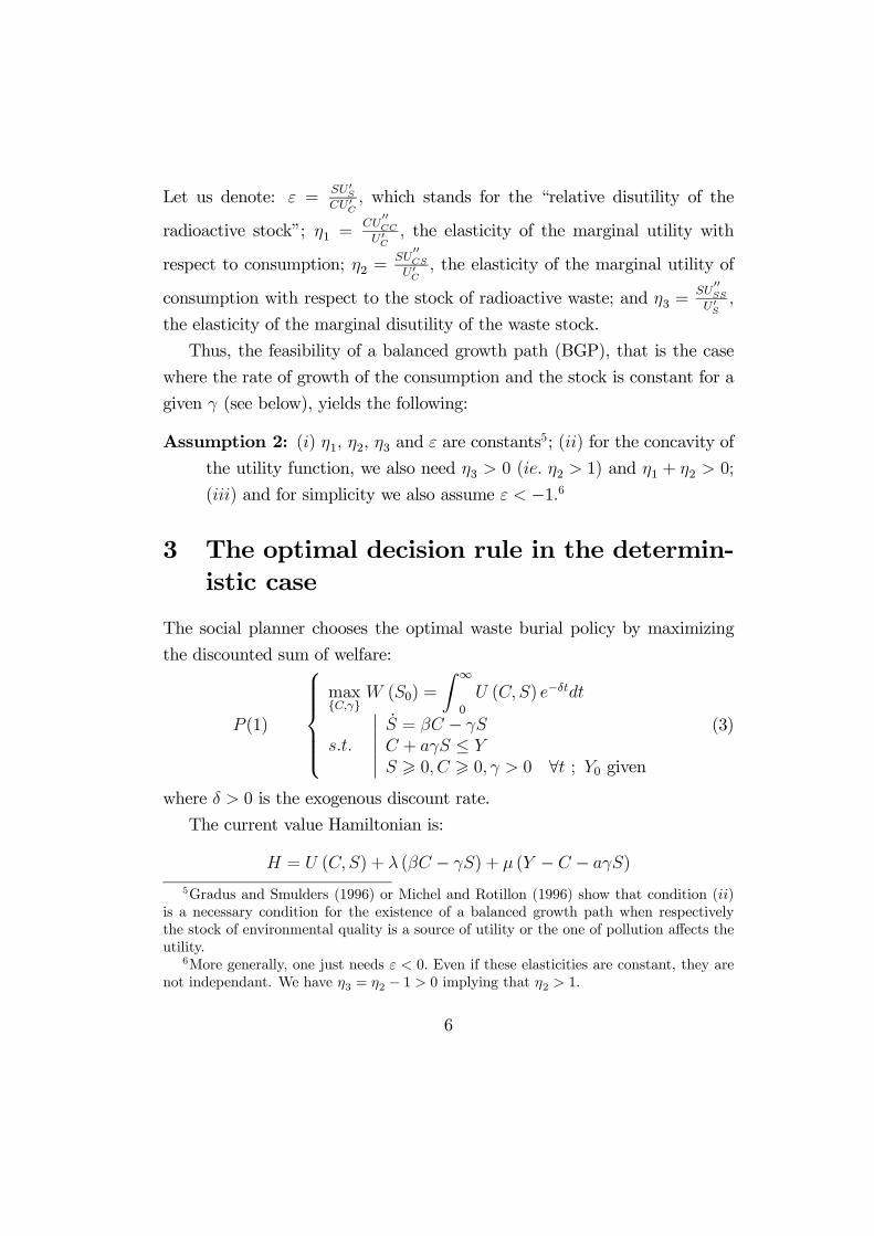
Let us denote: ε =SU 0SCU 0C

, which stands for the “relative disutility of the

radioactive stock”; η1 =CU

00CC

U 0C, the elasticity of the marginal utility with

respect to consumption; η2 =SU

00CS

U 0C, the elasticity of the marginal utility of

consumption with respect to the stock of radioactive waste; and η3 =SU

00SS

U 0S,

the elasticity of the marginal disutility of the waste stock.

Thus, the feasibility of a balanced growth path (BGP), that is the case

where the rate of growth of the consumption and the stock is constant for a

given γ (see below), yields the following:

Assumption 2: (i) η1, η2, η3 and ε are constants5; (ii) for the concavity ofthe utility function, we also need η3 > 0 (ie. η2 > 1) and η1 + η2 > 0;

(iii) and for simplicity we also assume ε < −1.6

3 The optimal decision rule in the determin-istic case

The social planner chooses the optimal waste burial policy by maximizing

the discounted sum of welfare:

P (1)

max{C,γ}

W (S0) =

Z ∞

0

U (C, S) e−δtdt

s.t.

¯¯ S = βC − γSC + aγS ≤ YS > 0, C > 0, γ > 0 ∀t ; Y0 given

(3)

where δ > 0 is the exogenous discount rate.

The current value Hamiltonian is:

H = U (C,S) + λ (βC − γS) + µ (Y − C − aγS)

5Gradus and Smulders (1996) or Michel and Rotillon (1996) show that condition (ii)is a necessary condition for the existence of a balanced growth path when respectivelythe stock of environmental quality is a source of utility or the one of pollution affects theutility.

6More generally, one just needs ε < 0. Even if these elasticities are constant, they arenot independant. We have η3 = η2 − 1 > 0 implying that η2 > 1.

6

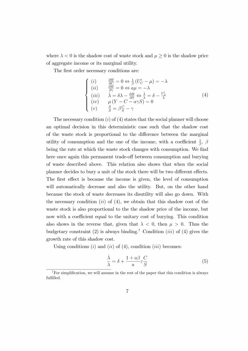
where λ < 0 is the shadow cost of waste stock and µ ≥ 0 is the shadow priceof aggregate income or its marginal utility.

The first order necessary conditions are:

(i) ∂H∂C= 0⇔ 1

β(U 0

C − µ) = −λ(ii) ∂H

∂γ= 0⇔ aµ = −λ

(iii) λ = δλ− ∂H∂S⇔ λ

λ= δ − U 0S

λ

(iv) µ (Y − C − aγS) = 0

(v) SS= βC

S− γ

(4)

The necessary condition (i) of (4) states that the social planner will choose

an optimal decision in this deterministic case such that the shadow cost

of the waste stock is proportional to the difference between the marginal

utility of consumption and the one of the income, with a coefficient 1β, β

being the rate at which the waste stock changes with consumption. We find

here once again this permanent trade-off between consumption and burying

of waste described above. This relation also shows that when the social

planner decides to bury a unit of the stock there will be two different effects.

The first effect is because the income is given, the level of consumption

will automatically decrease and also the utility. But, on the other hand

because the stock of waste decreases its disutility will also go down. With

the necessary condition (ii) of (4), we obtain that this shadow cost of the

waste stock is also proportional to the the shadow price of the income, but

now with a coefficient equal to the unitary cost of burying. This condition

also shows in the reverse that, given that λ < 0, then µ > 0. Thus the

budgetary constraint (2) is always binding.7 Condition (iii) of (4) gives the

growth rate of this shadow cost.

Using conditions (i) and (ii) of (4), condition (iii) becomes:

λ

λ= δ +

1 + aβ

aεC

S(5)

7For simplification, we will assume in the rest of the paper that this condition is alwaysfulfilled.

7

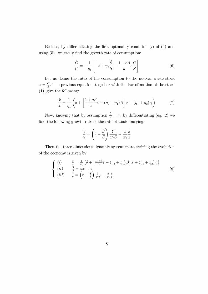
Besides, by differentiating the first optimality condition (i) of (4) and

using (5) , we easily find the growth rate of consumption:

C

C= − 1

η1

"−δ + η2

S

S− 1 + aβ

aεC

S

#(6)

Let us define the ratio of the consumption to the nuclear waste stock

x = CS. The previous equation, together with the law of motion of the stock

(1), give the following:

x

x=1

η1

µδ +

·1 + aβ

aε− (η2 + η1)β

¸x+ (η1 + η2) γ

¶(7)

Now, knowing that by assumption YY= r, by differentiating (eq. 2) we

find the following growth rate of the rate of waste burying:

γ

γ=

Ãr − S

S

!Y

aγS− x

aγ

x

x

Then the three dimensions dynamic system characterizing the evolution

of the economy is given by:(i) x

x= 1

η1

¡δ +

£1+aβa

ε− (η2 + η1)β¤x+ (η1 + η2) γ

¢(ii) S

S= βx− γ

(iii) γγ=³r − S

S

´YaγS− x

aγxx

(8)

8

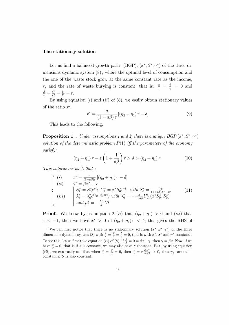
The stationary solution

Let us find a balanced growth path8 (BGP), (x∗, S∗, γ∗) of the three di-

mensions dynamic system (8) , where the optimal level of consumption and

the one of the waste stock grow at the same constant rate as the income,

r, and the rate of waste burying is constant, that is: xx= γ

γ= 0 and

SS= C

C= Y

Y= r.

By using equation (i) and (ii) of (8), we easily obtain stationary values

of the ratio x:

x∗ =a

(1 + aβ) ε[(η2 + η1) r − δ] (9)

This leads to the following.

Proposition 1 . Under assumptions 1 and 2, there is a unique BGP (x∗, S∗, γ∗)solution of the deterministic problem P (1) iff the parameters of the economy

satisfy:

(η2 + η1) r − ε

µ1 +

1

aβ

¶r > δ > (η2 + η1) r. (10)

This solution is such that :

(i) x∗ = a(1+aβ)ε

[(η2 + η1) r − δ]

(ii) γ∗ = βx∗ − r

(iii)

¯¯ S∗t = S∗0e

rt; C∗t = x∗S∗0ert; with S∗0 =

Y0(1+aβ)x∗−ar

λ∗t = λ∗0e(η2+η1)rt; with λ∗0 = − a

1+aβU 0C (x

∗S∗0 , S∗0)

and µ∗t = −λ∗ta∀t.

(11)

Proof. We know by assumption 2 (ii) that (η2 + η1) > 0 and (iii) that

ε < −1, then we have x∗ > 0 iff (η2 + η1) r < δ; this gives the RHS of

8We can first notice that there is no stationnary solution (x∗, S∗, γ∗) of the threedimensions dynamic system (8) with x

x =SS =

γγ = 0, that is with x

∗, S∗ and γ∗ constants.

To see this, let us first take equation (ii) of (8), if SS = 0 = βx−γ, then γ = βx. Now, if wehave x

x = 0, that is if x is constant, we may also have γ constant. But, by using equation

(iii), we can easily see that when xx =

SS = 0, then γ

γ = r Y0ert

aγS > 0, thus γt cannot beconstant if S is also constant.

9

condition (10). Now, we have γ∗ > 0 iff (η2 + η1) r− ε³1 + 1

aβ

´r > δ; which

is the LHS of the same condition.

Besides, knowing the values of x∗ and γ∗, it is easy to find the optimal

paths of waste stock and consumption. Let us first find the initial value of

the waste stock S0, as a function of the given initial income Y0. Knowing that

Yt = C∗t + aγ∗S∗t = (x∗ + aγ∗)S∗t = ((1 + aβ)x∗ − ar)S∗t and that along the

BGP SS= Y

Y= r, we can deduce that: S∗0 =

Y0(1+aβ)x∗−ar . We then have:

S∗t = S∗0ert for the waste stock; C∗t = x∗S∗0e

rt for consumption; and also, by

using (5), λ∗t = λ∗0e(η2+η1)rt with λ∗0 = − a

1+aβU 0C (x

∗S∗0 , S∗0) , for the shadow

cost of the waste stock and, with (4) (ii) we obtain µ∗t = −λ∗ta∀t, for the

shadow price of the aggregate income.

This proposition states the following for the deterministic solution, under

assumptions 1 and 2 and condition (10), which gives bounds on the discount

rate so as to obtain a BGP. First, if the discount rate increases, that is if

the social planner is more impatient, the ratio x∗ and also the optimal rate

of burying γ∗ will increase also ∂γ∗∂δ= β ∂x∗

∂δ> 0. Besides, if it is the growth

rate of the economy r which increases, x∗ and γ∗ will both decrease, we have∂x∗∂r

< 0 and ∂γ∗∂r= β ∂x∗

∂r− 1 < 0.

The optimal valuation of the waste stock

Moreover, knowing the values of x∗, S∗ and γ∗ along the BGP, we can

now find the optimal value of the objective function, that is the optimal

valuation of the initial waste stock in the deterministic case: W (S∗0) =Z ∞

0

U (x∗S∗0ert, S∗0e

rt) e−δtdt.

To obtain an analytical value of this valuation, we can specify, without

any loss of generality, a utility function of the CES form, suitable with as-

sumptions 1 and 2:

U (C, S) =(CSε)

1− 1σ

1− 1σ

(12)

where 0 < σ < 1 denotes the intertemporal elasticity of substitution for

10

consumption. We then have in this case U (.) < 0 and bounded from above,

η1 = − 1σ< 0, η2 = ε

¡1− 1

σ

¢= ε (1 + η1) > 0 (by assumption to still have

the “compensation effect”, that is why we need σ < 1, given that ε < −1,this assumption (σ < 1) is also sufficient in this case to ensure the concavity

of U (.)) and η3 = η2 − 1.Within this utility function, we show (see Appendix A (i)) that the opti-

mal valuation of the initial waste stock in the deterministic case is:

W (S∗0) = BU (x∗S∗0 , S∗0)

with B = −1r(1− 1

σ )(1+ε)−δ= −1

r(1+η1+η2)−δ which is assumed to be positive, such

that the valuation of the (“bad”) waste stock being negative. This implies

the following additional condition on the parameters of the economy: δ >

r (1 + η1 + η2) = r + r (η1 + η2) . Combining this condition with the one of

the existence of a stationary state given (10), we obtain a more restrictive

condition:

(η2 + η1) r − ε

µ1 +

1

aβ

¶r > δ > r + r (η1 + η2) (13)

4 The optimal waste burial policy under un-certainty

We assume that there is a possibility that at a given future date T, an accident

occurs with a probability p ∈ [0, 1] which implies the destocking of a quantityS. For simplification, we also assume that this quantity is proportional to

the existing waste stock S = θS(3)T , where S(3)T is the level of the remaining

waste stock just before the accident occurs and θ ≥ 0. Besides, we assumethat the destocking is a once and for all phenomenon. Thus the level of the

waste stock just after the accident has occurred, S(2)T , is given by:

S(2)T =

S(2)T = (1 + θ)S

(3)T with probability p

S(3)T with proba. 1− p

(14)

11

thus, with the probability p, the stock after time T will be the one remaining

before the accident plus a part θ and with a probability (1− p) this stock

will remain as before the accident.

4.1 The model after the occurrence of the nuclear ac-cident

After the nuclear waste stock accident has occurred, the problem is the same

as the one of certainty P (1), the only difference is the initial level of the

radioactive waste stock.

The state valuation function of a given remaining stock S(2)T from time T

onwards is therefore given as follows:

P (2)

maxγ(2)t

W³S(2)T

´=R∞T

U³C(2)t , S

(2)t

´e−δ(t−T )dt

s.t.

¯¯ S

(2) = βC(2) − γ(2)S(2)

C(2) = Y − aγ(2)S(2)

S(2)t , C

(2)t , γ(2) > 0, ∀t > T

YT given

By analogy, with the solution of the problem P (1) above, we know that

the economy will keep the same growth path, with x(2) = x∗ and γ(2) = γ∗.

It inherits a level of the waste stock S(2)T , and depending on this stock, that

is on the realization of the uncertainty (the occurrence of the accident), we

also obtain the following along the new BGP from time T onwards:C(2)t

C(2)t

=S(2)t

S(2)t

= r;S(2)t = S

(2)T er(t−T );C(2)

t = x∗S(2)t ∀t = [T,+∞[.

4.2 The model with uncertainty

As we have assumed that there is a possibility that at a given future date T,

an accidental destocking occurs which changes the waste stock in an unknown

12

level, the program of the social planner writes (see Dasgupta and Heal; 1974):

P (3)

maxγ(3)t

Z T

0

U³C(3)t , S

(3)t

´e−δtdt+ e−δTEW

³S(2)T

´

s.t.

¯¯ S

(3) = βC(3) − γ(3)S(3)

C(3) = Y − aγ(3)S(3)

S(3)t , C

(3)t , γ(3) > 0, ∀t > T

Y0 given

where the mathematical expectation of the remaining stock at time T, just

after the accident has occurred, i.e. the expected negative bequest for the

future generations is

EW³S(2)T

´= pW

³S(2)T

´+ (1− p)W

³S(3)T

´. (15)

The first order necessary conditions of this problem P (3) are the same

as those of the one of the deterministic case P (1) , that is when there is

no accident. The dynamic system, in¡x(3), S(3), γ(3)

¢, characterizing the

evolution of the economy before the accident occurs is then still (8). However,

we must add the following transversality condition:

λ(3)T =

∂EW³S(2)T

´∂S

(2)T

(16)

This transversality condition states that when the accident occurs, the

shadow cost of the waste stock must be equal to the expected marginal

negative value of the remaining (existing) stock.

We first know from the first order conditions (4) that λ(3)T = −U 0C x(3)S(3)T ,S

(3)T −µ(3)T

β,

with µ(3)T = −λ(3)0

ae(η1+η2)rT .We also show (see Appendix A (ii)), by using the

utility function given in (12), that∂W S

(2)T

∂S(2)T

= B [1 + ε]x∗U 0C

³x∗S(2)T , S

(2)T

´,

when the accident occurs at time T, and∂W S

(3)T

∂S(3)T

= B [1 + ε]x∗U 0C

³x∗S(3)T , S

(3)T

´when there is no accident at this time. Knowing also that by assumption

13

S(2)T = (1 + θ)S

(3)T , the RHS of (16) , that is the expected marginal value of

the waste stock at time T, is given by:

∂EW³S(2)T

´∂S

(2)T

= B [1 + ε]x∗hpU 0

C

³x∗ (1 + θ)S

(3)T , (1 + θ)S

(3)T

´+ (1− p)U 0

C

³x∗S(3)T , S

(3)T

´i(17)

and the transversality condition (16) therefore becomes:

−U 0C

³x(3)S

(3)T , S

(3)T

´β

− λ(3)0

aβe(η1+η2)rT =

∂EW³S(2)T

´∂S

(2)T

(18)

The stationary solution

Knowing the solution of the problem P (1) above, to show that there is a

unique solution to this problem P (3) with uncertainty, we only have to show

that there exists a unique value x(3) satisfying this transversality condition.

This leads to the following.

Proposition 2 . Under assumptions 1 and 2 and given condition (13), thereis a unique BGP

¡x(3), S(3), γ(3)

¢solution of the problem with uncertainty

P (3), which is such that :

(i) x(3) = x∗h1− [1 + ε]Bβx∗p

h(1 + θ)(η2+η1) − 1

ii 1η1

(ii) γ(3) = βx(3) − r

(iii)

¯¯¯S(3)t = S

(3)0 ert; C

(3)t = x(3)S

(3)0 ert; ∀t ∈ [0, T ]

with S(3)0 = Y0(1+aβ)x(3)−ar

λ(3)t = λ

(3)0 e(η2+η1)rt and µ(3)t = −λ

(3)t

a∀t ∈ [0, T ]

with λ(3)0 = −aβ³B [1 + ε]x∗ + 1

β

´U 0C

³x(3)S

(3)0 , S

(3)0

´(19)

Proof. First, as we have seen, the necessary conditions are the same inproblems P (1) and P (3), apart from the transversality condition (18). We

14

also know that this transversality condition must hold for any value of the

probability p between 0 and 1. Besides, if p = 0, as in the deterministic

case, the optimal choice of the social planner will be to choose x(3) = x∗.

Thus, setting p = 0 and x(3) = x∗ in (18) allows us to find the value of the

initial shadow cost of the waste stock (see Appendix B for details): λ(3)0 =

−aβ³B [1 + ε]x∗ + 1

β

´U 0C

³x(3)S

(3)0 , S

(3)0

´.

Now, reintroducing this value of λ(3)0 , which depends on the distribution

of probability of an accident only by the level of the initial marginal utility

of consumption, in the transversality condition (18) and using the utility

function given in (12), we easily show, after few manipulations, that: x(3) =

x∗h1− [1 + ε]Bβx∗p

h(1 + θ)(η2+η1) − 1

ii 1η1 . We therefore can obtain the

optimal value of the rate of waste burying: γ(3) = βx(3) − r. Also, with

the same routine that we used before (see the Proof of proposition 1), we

can compute the optimal path of consumption and waste stock before the

accident occurs.

A comparison with the deterministic solution

We now come to one of the main motivation of this paper: will the un-

certainty change the behavior of the central planner in a trivial and intuitive

way? The common sense would tell us that burying should decrease with the

risk of an accident.

Let us rewrite the optimal level of the ratio x in the case of uncertainty,

given in equation (i) of (19) as follows:µx(3)

x∗

¶η1

= 1− [1 + ε]| {z }−

Bβx∗p| {z }+

h(1 + θ)(η1+η2) − 1

i| {z }

+

> 1

we see that we always have x∗ > x(3) and given the relation between x and

γ in both case, γ = βx− r, we also have γ(3) < γ∗. So, as the common sense

tell us, the introduction of uncertainty would lead to a choice of a lower rate

15

of waste burying. The social planner chooses to limit the largeness of the

accident.

But, we also know that, at any time t, along these two BGP, the one with

uncertainty and the one without, because the level of income is exogenously

given, the level of the waste stock is a decreasing function of the ratio x:

St =Yt

(1+aβ)x−ar . The introduction of uncertainty leads to a higher accumula-

tion of the nuclear waste, that is to a higher level of the waste stock. This

corresponds to a higher disutility for the household.

Because the introduction of uncertainty does not change the rate of bury-

ing and the level of the stock in the same direction, its effect on the evolution

of the optimal consumption is not trivial. Basically, we have the static budget

constraint Y = C + aγS which implies:

dC = −µdγ−+ dS

+

¶When the rate of burying decreases and, in the same time, the stock of waste

increases, the evolution of the flow of buried waste γS, and also the one of the

total cost of burying aγS, and therefore the one of the optimal consumption

will depend on the relative change of the two variables. And the determinants

of this trade-off are those of the optimal burying rateµδ−, p−, θ, r, a, ε, σ

¶. This

property on the opposite evolution of γ and S implies that the total amount

of buried waste is also ambiguous. So, even if the social planner faces an

uncertainty on the safety of the burial policy, the total amount of buried

waste may increase.

5 Conclusion

The issue addressed in this paper concerns the management of the increas-

ing nuclear waste stock. We analyze the optimal nuclear waste burial policy

under an uncertainty: the possibility that an accident might occur in the fu-

ture. In a simple optimal growth framework, we consider two waste process

16

solutions: temporary storage or burying of waste. We show, under some

conditions on the waste burial policy, that nuclear power may be a long-term

solution for the world energy demand. This solution consist in burying a

constant part of the waste stock, in the deterministic case as well as in the

uncertain case. Under uncertainty on the future safety of the buried waste,

the social planner will decide to decrease the rate of waste burying, but the

evolution of consumption and hence of the level of buried waste are ambigu-

ous. Namely (and counter-intuitively), depending on some simple conditions

on the balanced growth rate of the economy and on the preferences parame-

ters of the households, optimal consumption, and then optimal amount of

buried waste, may increase even under a risk of accident in the future.

References

Ayong Le Kama A., (2001) "Preservation and exogenous uncertain future

preferences", Economic Theory, vol. 18, pp. 745-752.

Ayong Le Kama A., Schubert K., (2004), “Growth, Environment and Un-

certain Future Preferences”, Environmental and Resource Economics, 28, p.

31-53.

Ayong Le Kama A., Schubert K., (2006), "Ressources renouvelables et incer-

titude sur les préférences des générations futures", Revue d’Economie Poli-

tique, n◦2, pp. 229-250.

Chakravorty U., Magne B., Moreaux M., (2006), "Can Nuclear Power solve

the Global Warming Problem?", IDEI Working Paper, 381.

Dasgupta P.S., Heal G., (1974), “The Optimal Depletion of Exhaustible Re-

sources”, Review of economic studies, vol. 41, p. 1-28.

Gradus S., Smulders S., (1996), “Pollution Abatement and Long-termGrowth”,

European Journal of Political Economy, 12, p. 505—532.

17

Hartwick J., (1977), “Intergenerational Equity and the Investing of Rents

from Exhaustible Resources”, American Economic Review, 67, p. 972-974.

Heal G. M., (1993), “The Optimal Use Of Exhaustible Resources”, in Hand-

book of Natural Resource and Energy Economics, vol. III, A.V. Kneese and

J.L. Sweeney (Eds), Elsevier Science Publishers.

Hotteling H., (1931), “The Economics of Exhaustible Resources”, The Jour-

nal of Political Economy, vol. 39, n◦2, p. 137-175.

Michel P., Rotillon G., (1995), “Disutility of Pollution and Endogenous

Growth”, Environmental and Resource Economics, vol. 6(3), p. 279—300.

Van der Ploeg F., Withagen C., (1991), “Pollution Control and the ramsey

Problem”, Environmental and Resource Economics, 1, p. 215-236.

Whipple C.G. (1996), “Can Nuclear Waste Be Stored at Yucca Mountain?”,

Scientific American, vol. 274, p. 72-80.

Appendix

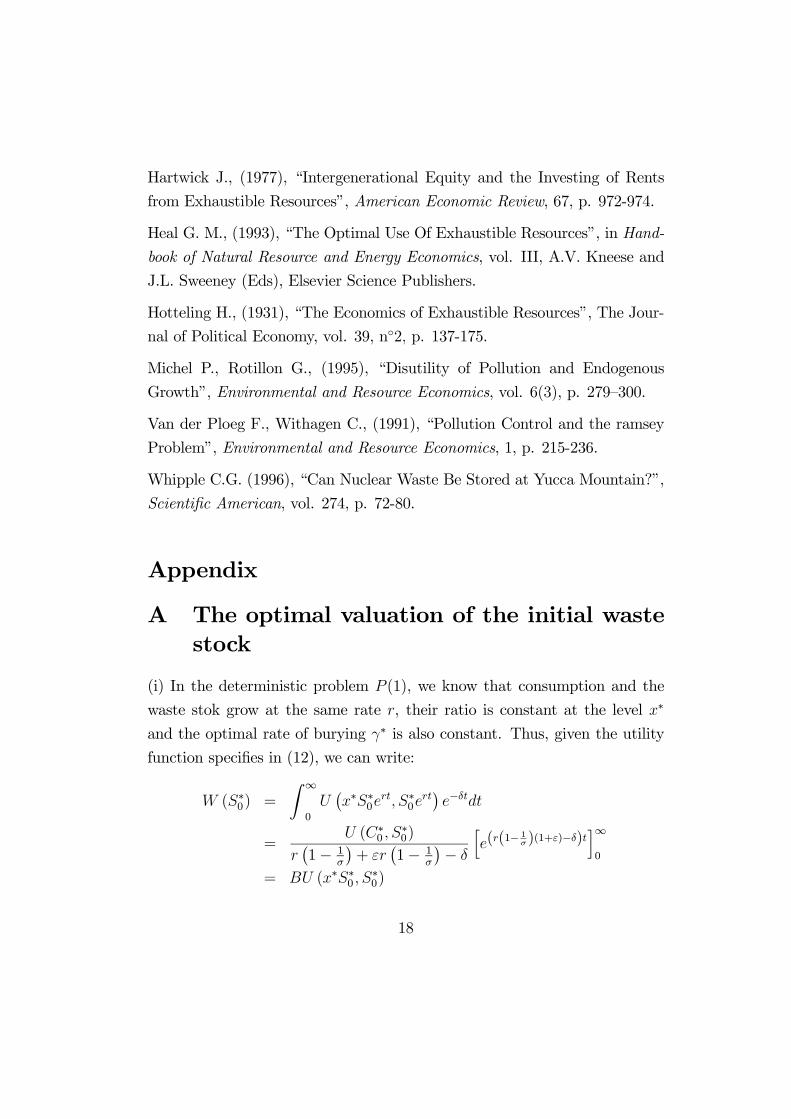
A The optimal valuation of the initial wastestock

(i) In the deterministic problem P (1), we know that consumption and the

waste stok grow at the same rate r, their ratio is constant at the level x∗

and the optimal rate of burying γ∗ is also constant. Thus, given the utility

function specifies in (12), we can write:

W (S∗0) =

Z ∞

0

U¡x∗S∗0e

rt, S∗0ert¢e−δtdt

=U (C∗0 , S

∗0)

r¡1− 1

σ

¢+ εr

¡1− 1

σ

¢− δ

he(r(1−

1σ )(1+ε)−δ)t

i∞0

= BU (x∗S∗0 , S∗0)

18

with B = −1r(1− 1

σ )(1+ε)−δ= −1

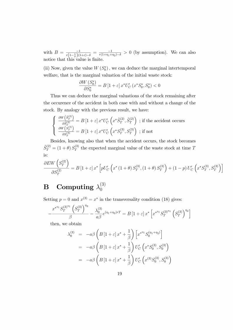
r(1+η1+η2)−δ > 0 (by assumption). We can also

notice that this value is finite.

(ii) Now, given the value W (S∗0) , we can deduce the marginal intertemporal

welfare, that is the marginal valuation of the initial waste stock:

∂W (S∗0)∂S∗0

= B [1 + ε]x∗U 0C (x

∗S∗0 , S∗0) < 0

Thus we can deduce the marginal valuations of the stock remaining after

the occurence of the accident in both case with and without a change of the

stock. By analogy with the previous result, we have:∂W S

(2)T

∂S(2)T

= B [1 + ε]x∗U 0C

³x∗S(2)T , S

(2)T

´; if the accident occurs

∂W S(3)T

∂S(3)T

= B [1 + ε]x∗U 0C

³x∗S(3)T , S

(3)T

´; if not

Besides, knowing also that when the accident occurs, the stock becomes

S(2)T = (1 + θ)S

(3)T the expected marginal value of the waste stock at time T

is:

∂EW³S(2)T

´∂S

(2)T

= B [1 + ε]x∗hpU 0

C

³x∗ (1 + θ)S

(3)T , (1 + θ)S

(3)T

´+ (1− p)U 0

C

³x∗S(3)T , S

(3)T

´i

B Computing λ(3)0

Setting p = 0 and x(3) = x∗ in the transversality condition (18) gives:

−x∗

η1S(3)η1

T

³S(3)T

´η2β

− λ(3)0

aβe(η1+η2)rT = B [1 + ε]x∗

hx∗

η1S(3)η1

T

³S(3)T

´η2ithen, we obtain

λ(3)0 = −aβ

µB [1 + ε]x∗ +

1

β

¶hx∗

η1S(η1+η2)0

i= −aβ

µB [1 + ε]x∗ +

1

β

¶U 0C

³x∗S(3)0 , S

(3)0

´= −aβ

µB [1 + ε]x∗ +

1

β

¶U 0C

³x(3)S

(3)0 , S

(3)0

´19