Optimal Monetary Policy Rules in an Estimated

Sticky-Information Model

Ricardo Reis�

Columbia University

October 2008

Abstract

This paper uses a dynamic stochastic general-equilibrium (DSGE) model with sticky

information as a laboratory to study monetary policy. It characterizes the model�s pre-

dictions for macro-dynamics and optimal policy at prior parameters, and then uses data

on �ve U.S. macroeconomic series to update the parameters and provide an estimated

model that can be used for policy analysis. The model answers a few policy questions:

How does sticky information a¤ect optimal monetary policy? What is the optimal

interest-rate rule? What is the optimal elastic price-level targeting rule? How does

parameter uncertainty a¤ect optimal policy? Are the conclusions for the Euro-area

di¤erent?

JEL classi�cation: E52, E32, E10

�I am grateful to Olivier Blanchard and an anonymous referee for comments and to Tiago Berriel forexcellent research assistance.

1

1 Introduction

Many (or perhaps most) models that macroeconomists use are intended to inform policy.

Most of the times, this takes the form of simple models that either qualitatively highlight

a particular mechanism, or quantitatively suggest some guiding principles. More rarely,

macroeconomists write models that try to systematically account for the dynamics of the

many variables that policymakers care about, and that can give concrete policy advice.

Recently, the progress in building, estimating and analyzing dynamic stochastic general

equilibrium models (DSGEs) that followed Smets and Wouters�s (2003) work has led to an

e¤ort to give this more ambitious form of policy advice. Following on the footsteps of Taylor

(1979), work by Schmitt-Grohe and Uribe (2007), Levin et al (2006), Juillard et al (2006)

and others estimated DSGE models using several macroeconomic series and used them for

policy advice. There are a few advantages to using these models to study policy. First,

they provide a coherent account of the many macroeconomic series that policymakers care

about. Second, they emphasize the role of expectations and optimal behavior in response

to di¤erent policy rules. And third, because uncertainty is dealt with probabilistically, one

can assess the robustness of the conclusions in a systematic way.

All of the papers just mentioned use variants of the Christiano et al (2005) model,

with many rigidities impeding adjustment, from sticky (but indexed) prices and wages to

habits in consumption. This paper presents an alternative DSGE model of macroeconomic

�uctuations, in which there is only one departure from a classical benchmark that applies

to all markets: sticky information. At any date, only a fraction of consumers, workers and

�rms update their information and make plans for consumption, wages and prices for the

future.

After presenting the model, I choose its parameter values to match the conventions

that have emerged from prior studies, and study the dynamics properties of the model

and is policy implications. In particular, I examine the impact that sticky information in

di¤erent markets has on the response to monetary policy shocks and on optimal instrument

and targeting rules. Comparing the di¤erences in impulse response and optimal policies

as information stickiness changes characterizes the impact of informational frictions on

monetary policy.

Next, I update the parameter values to take into account uncertainty in a Bayesian sense

2

using U.S. data since 1986. The contrast in the impulse responses to shocks at the prior and

posterior parameters provides further insights into the properties of the model. Moreover,

the model can then be used to provide concrete guidance to policymakers. I investigate

which are the optimal interest-rate and price-targeting rules, as well as their robustness

to parameter estimates, by calculating robustly-optimal (in the sense of Bayesian model-

averaging) policy rules and by repeating the analysis for the Euro-area.

The motivation for this work is twofold. First, there is still an active debate on the

merits and �aws of di¤erent models of rigidities. By characterizing optimal policy in a

model that is quite di¤erent from the ones where optimal policy has been studied so far,

this paper provides both a check on which policy prescriptions are robust across models of

rigidities, as well as a contrast between the monetary transmission mechanisms in di¤erent

models.

Second, sticky-information models are interesting in their own right, but monetary policy

has only been studied analytically in simple models where only price-setters are inattentive

(Ball et al, 2005, Branch et al, 2007). This paper provides the �rst systematic study

of optimal monetary policy in a medium-scale model with pervasive sticky information

estimated to mimic the features of the U.S. data. The model was �rst sketched in Mankiw

and Reis (2006, 2007), and is further explored in a companion paper to this one, Reis (2008),

that presents the micro-foundations in detail, the algorithms that solve it, and the sensitivity

of estimates to di¤erent speci�cations. This paper uses this theoretical framework to study

concrete policy questions.

The paper is organized as follows. Section 2 presents the model, starting with the

classical general-equilibrium benchmark and its �exible equilibrium, and then introducing

sticky information. Section 3 picks parameters using priors, and discusses the role of

information frictions on the dynamics of the model and on optimal monetary policy. Section

4 updates the parameter values using data for the United States, discuses the �t of the

models to the data, and answers several questions on optimal monetary policy through the

lenses of the estimated DSGE model. Section 5 discusses the robustness of the results to

alternative parameter speci�cations, and section 6 compares the policy conclusions reached

with the results in the literature. Section 7 concludes by stating the lessons from these

experiments for monetary policy.

3

2 The model

This section starts by presenting a simple classical model of �uctuations. The �rst part

describes the environment, agents and markets, and the second interprets the key reduced-

form equilibrium relations that characterize the equilibrium in aggregate variables. Because

the model is relatively standard, readers familiar with it may skip the environment and

jump to the reduced-form equations directly. The third part characterizes the equilibrium

dynamics in this model, and the fourth part introduces sticky information and derives its

associated reduced-form equilibrium equations.

2.1 The environment

I consider a world with three types of market, for goods, labor and savings, and three types

of rational agents, consumers, workers, and �rms.

A household is made of a consumer and a worker, and there is a continuum of each

indexed by j and k respectively in the unit interval.1 Each household�s utility function is:

Et

1Xt=0

�t

0@ln(Ct;j)� {L1+1= t;k

1 + 1=

1A ; (1)

where Ct;j and Lt;k are consumption and hours worked respectively, and the parameters

�; , and { are the discount factor, the Frisch elasticity of labor supply, and the relative

disutility of working respectively. Consumption is a Dixit-Stiglitz aggregator of varieties

with random elasticity of substitution ~�t:

Ct;j =

�Z 1

0Ct;j(i)

~�t~�t�1di

� ~�t�1~�t

(2)

The household�s budget constraint is:

Mt+1;j = �t+1 (Mt;j � Ct;j + (1� �w)Wt;kLt;k=Pt + Tt;j) ; (3)

where Mt;j is real wealth and �t+1 is the real interest rate on bonds. Consumers meet each

other to trade these bonds in the savings market, where bonds are in zero net supply. The

1 I separate worker and consumer because in the models with frictions, they may di¤er in their constraints.In the classical case though, one can think of the household making all decisions together.

4

consumer makes purchases in the goods market, and Pt is the static cost-of-living index

associated with (2), so thatR 10 Pt;iCt;j(i) = PtCt;j and Pt =

�R 10 P

1�~�tt;i di

�1=(1�~�t). The

worker sells its unique type of di¤erentiated labor in the labor market in return for nominal

wageWt;k after a tax on labor income �w. Finally, the household receives Tt;j , which are the

pro�ts from owning �rms, lump-sum transfers from the government, and payments from an

insurance contract that all households signed at the beginning of time when they were all

ex ante identical, ensuring that they have the same wealth at all dates.

There is a continuum of �rms in the unit interval indexed by i. They assemble the

varieties of labor into composite labor Nt;i through a Dixit-Stiglitz aggregator:

Nt;i =

�Z 1

0Nt;i(k)

~ t~ t�1dk

� ~ t�1~ t

; (4)

with random elasticity of substitution ~ t. The cost of hiring labor isWtNt;i =R 10 Wt;kNt;i(k)dk

given the static wage index Wt =�R 10 W

1�~ tt;k dk

�1=(1�~ t). The labor input is then trans-

formed through a diminishing-returns to scale technology to produce variety of good i,

Yt;i = AtN�t;i, where � is the degree of returns to scale, and At is a common technology

shock. The �rm is a monopolist that chooses the price of its good Pt;i and pays a sales tax

�p, so that real pro�ts are:

[(1� �p)Pt;iYt;i �WtNt;i] =Pt (5)

Finally, the government intervenes in the economy �scally by charging taxes and by

buying a random share 1�1=Gt of the goods in the market. These governmental purchases

are wasted, and I refer to them broadly as aggregate demand shocks. The surpluses or

de�cits are rebated/charged to the households in a lump-sum way. A Central Bank supplies

reserves to the bond market and because it can generate reserves at will, it can target the

nominal interest rate it � log [Et (�t+1Pt+1=Pt)]. Monetary policy follows a Taylor rule

with exogenous shocks "t:

it = �p log(Pt=Pt�1) + �y log(Yt=Yct )� "t. (6)

In this expression, Y ct refers to the classical equilibrium so the second term is always zero

in this economy, while in the �rst term �p > 1 to satisfy the Taylor principle.

5

Having described the agents, I now turn to the equilibrium in each market. In the savings

market, each consumer is choosing Ct;j to maximize (1) subject to (3) and a no-Ponzi game

condition. The standard consumption Euler equation is:

C�1=�t;j = �Et

h�t+1C

�1=�t+1;j

i(7)

In the market for good i, the demand by each individual consumer comes from choosing

Ct;j(i) to maximize (2) subject to some total expenditure PtCt;j . Aggregating over all

consumers, and taking into account government spending, the total demand for good i is:

Yt;i = (Pt;i=Pt)�~�t Gt

Z 1

0Ct;jdj: (8)

The producer of good i in turn chooses the price Pt;i to maximize (5) subject to the pro-

duction function and the demand (8). The �rst-order condition is:

Pt;i = (1� �p)��

~�t~�t � 1

���WtNt;i

�Yt;i

�: (9)

Prices are the multiple of three terms: the after-tax share of sales, a desired markup, and

marginal cost, which equals the wage divided by the marginal product of labor (which here

equals output per hour times �).

In the market for labor variety j, each �rm minimizes total costs WtNt;i subject to the

aggregator (4). Integrating over all �rms leads to the demand for variety k:

Lt;k = (Wt;k=Wt)�~ t

Z 1

0Nt;idi. (10)

Workers choose the nominal wage to charge Wt;k in order to maximize utility (1) subject

to the budget constraint (3), a no-Ponzi game condition, and the demand for their variety

(10). The Euler equation is:

�~ t

~ t � 1

��L1= t;k Pt

Wt;k= �Et

0@�t+1 � � ~ t+1~ t+1 � 1

��

0@L1= t+1;kPt+1

Wt+1;k

1A1A : (11)

If ~ t is �xed, this condition states that the marginal disutility of supplying labor today

(L1= t;k ) divided by the real wage (Wt;k=Pt) is equated to the discounted marginal disutility

6

tomorrow (L1= t+1;k) divided by the real wage tomorrow (Wt+1;k=Pt+1) times the real interest

rate. With time-varying ~ t, the Euler equation takes into account the change in the markup

that the monopolistic worker wants to charge.

To conclude, the optimality conditions above describe a monopolistically competitive

equilibrium of a simple classical economy. There are �ve source of shocks in this economy

to: productivity (At), aggregate demand (Gt), price and wage markups (~�t and ~ t), and

monetary policy ("t). I will focus on explaining the dynamics of �ve variables: goods�

price in�ation (Pt=Pt�1), output growth (Yt=Yt�1 =R 10 Yt;idi=

R 10 Yt�1;idi), hours worked

(Lt =RLt;kdk), real wage growth ((Wt=Pt) = (Wt�1=Pt�1)), and nominal interest rates (it).

2.2 The reduced-form expressions

Log-linearizing all variables around the non-stochastic Pareto-optimum steady state of this

economy leads to �ve aggregate relations.

Starting with the aggregate production function, adding over all the log-linear produc-

tion functions gives:

yt = at + �lt; (12)

relating total output (yt) to productivity shocks (at) and hours worked (lt) subject to

decreasing returns to scale with labor share �.

Turning to the aggregate supply relation (or Phillips curve), from the optimal behavior

of the identical �rms, their desired price p�t equals:

p�t = pt +�(wt � pt) + (1� �)yt � at

� + �(1� �) � ��t(� � 1)[� + �(1� �)] (13)

This equation states that desired prices equal the price level plus real marginal costs and

desired markups. Real marginal costs rise with the cost of the labor input, real wages

(wt � pt), as well as with output (yt), because of decreasing returns to scale, and fall with

productivity (at). The desired markup rises whenever the random substitutability of goods�

varieties decreases (�t), where � is the steady-state elasticity of substitution for goods.

Third, because all the consumers are identical, the Euler equation for output (or IS

curve) is:

yt � gt = �(it � Et�pt+1) + Et [yt+1 � gt+1] : (14)

7

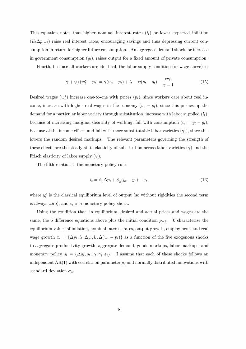
This equation notes that higher nominal interest rates (it) or lower expected in�ation

(Et�pt+1) raise real interest rates, encouraging savings and thus depressing current con-

sumption in return for higher future consumption. An aggregate demand shock, or increase

in government consumption (gt), raises output for a �xed amount of private consumption.

Fourth, because all workers are identical, the labor supply condition (or wage curve) is:

( + ) (w�t � pt) = (wt � pt) + lt � (yt � gt)� t � 1 (15)

Desired wages (w�t ) increase one-to-one with prices (pt), since workers care about real in-

come, increase with higher real wages in the economy (wt � pt), since this pushes up the

demand for a particular labor variety through substitution, increase with labor supplied (lt),

because of increasing marginal disutility of working, fall with consumption (ct = yt � gt),

because of the income e¤ect, and fall with more substitutable labor varieties ( t), since this

lowers the random desired markups. The relevant parameters governing the strength of

these e¤ects are the steady-state elasticity of substitution across labor varieties ( ) and the

Frisch elasticity of labor supply ( ).

The �fth relation is the monetary policy rule:

it = �p�pt + �y(yt � yct )� "t; (16)

where yct is the classical equilibrium level of output (so without rigidities the second term

is always zero), and "t is a monetary policy shock.

Using the condition that, in equilibrium, desired and actual prices and wages are the

same, the 5 di¤erence equations above plus the initial condition p�1 = 0 characterize the

equilibrium values of in�ation, nominal interest rates, output growth, employment, and real

wage growth xt = f�pt; it;�yt; lt;�(wt � pt)g as a function of the �ve exogenous shocks

to aggregate productivity growth, aggregate demand, goods markups, labor markups, and

monetary policy st = f�at; gt; �t; t; "tg. I assume that each of these shocks follows an

independent AR(1) with correlation parameter �s and normally distributed innovations with

standard deviation �s.

8

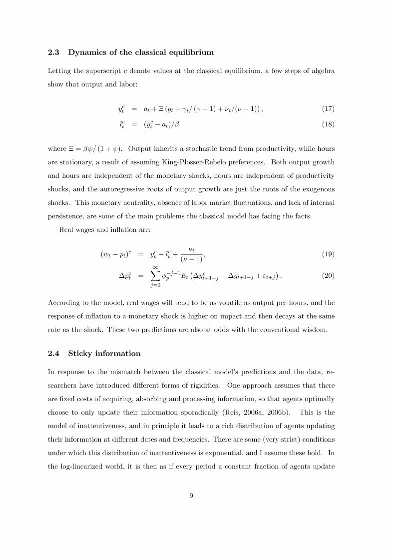
2.3 Dynamics of the classical equilibrium

Letting the superscript c denote values at the classical equilibrium, a few steps of algebra

show that output and labor:

yct = at + �(gt + t= ( � 1) + �t=(� � 1)) ; (17)

lct = (yct � at)=� (18)

where � = � = (1 + ). Output inherits a stochastic trend from productivity, while hours

are stationary, a result of assuming King-Plosser-Rebelo preferences. Both output growth

and hours are independent of the monetary shocks, hours are independent of productivity

shocks, and the autoregressive roots of output growth are just the roots of the exogenous

shocks. This monetary neutrality, absence of labor market �uctuations, and lack of internal

persistence, are some of the main problems the classical model has facing the facts.

Real wages and in�ation are:

(wt � pt)c = yct � lct +�t

(� � 1) ; (19)

�pct =1Xj=0

��j�1p Et��yct+1+j ��gt+1+j + "t+j

�: (20)

According to the model, real wages will tend to be as volatile as output per hours, and the

response of in�ation to a monetary shock is higher on impact and then decays at the same

rate as the shock. These two predictions are also at odds with the conventional wisdom.

2.4 Sticky information

In response to the mismatch between the classical model�s predictions and the data, re-

searchers have introduced di¤erent forms of rigidities. One approach assumes that there

are �xed costs of acquiring, absorbing and processing information, so that agents optimally

choose to only update their information sporadically (Reis, 2006a, 2006b). This is the

model of inattentiveness, and in principle it leads to a rich distribution of agents updating

their information at di¤erent dates and frequencies. There are some (very strict) conditions

under which this distribution of inattentiveness is exponential, and I assume these hold. In

the log-linearized world, it is then as if every period a constant fraction of agents update

9

their information and write plans into the future that they revise only when they obtain

information again. This is the model of sticky information, where information disseminates

slowly throughout the population.

In the context of the general equilibrium model presented so far, there is sticky informa-

tion in all three markets. While consumers and workers share a household, in the sense of

having the same utility function and facing the same budget constraint, and the household

owns the �rms, these three agents may have di¤erent information. When the consumer

updates his information, he learns about what the worker in his household has been up to

and about the �rms�pricing plans, and then makes his own choices of a consumption plan.

This model, where inattentiveness is pervasive in all markets is the sticky information in

general equilibrium model (SIGE).2

In the goods markets, �rms update their information at rate �, so there are � �rms with

current information, �(1 � �) with 1-period old information, �(1 � �)2 with 2-period old

information, and so on. Letting the index i denote the group of �rms that last updated

their information i periods ago, then it will set its price for date t equal to what it expected

its desired price would be: pt;i = Et�i(p�t ).3 The sticky-information Phillips curve then is:

pt = �1Xi=0

(1� �)iEt�i�pt +

�(wt � pt) + (1� �)yt � at� + �(1� �) � ��t

(� � 1)[� + �(1� �)]

�(21)

In the savings market, there is sticky information on the part of the consumers, which

update their information at rate �, so that a share �(1 � �)j of consumers last updated

its information s periods ago. After iterating the Euler equation for desired consumption

forward, and de�ning a measure of wealth yc1 = lim�!1Et (yt+� ), and the long real interest

rate Rt = EtP1

�=0 (it+� ��pt+1+� ), we obtain the sticky-information IS curve:

yt = �1Xj=0

(1� �)jEt�j (yn1 � �Rt) + gt; (22)

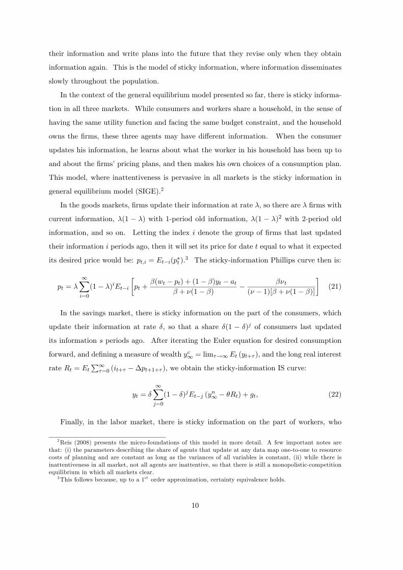
Finally, in the labor market, there is sticky information on the part of workers, who

2Reis (2008) presents the micro-foundations of this model in more detail. A few important notes arethat: (i) the parameters describing the share of agents that update at any data map one-to-one to resourcecosts of planning and are constant as long as the variances of all variables is constant, (ii) while there isinattentiveness in all market, not all agents are inattentive, so that there is still a monopolistic-competitionequilibrium in which all markets clear.

3This follows because, up to a 1st order approximation, certainty equivalence holds.

10

update their information at rate !. Following similar steps as in the consumption case, the

sticky information wage curve is:

wt = !

1Xk=0

(1� !)kEt�k�pt +

(wt � pt) +

+lt

+ + (yc1 �Rt)

+ � t( + )( � 1)

�(23)

These three equations, together with the production function (12) and the policy rule

(16), plus the relevant initial conditions, de�ne the SIGE equilibrium.

3 Dynamics and optimal policy with sticky information

Making the model useful for policy analysis requires �rst picking a set of parameters that

make it mimic some features of the data, then understanding its dynamic properties, and

�nally performing counterfactual policy experiments.

3.1 Data and prior parameters

The model assumed a closed economy with an unchanged monetary policy rule and un-

changed variances so that the fractions of agents adjusting was constant. These features lead

me to focus on seasonally-adjusted quarterly data for a large economy, the United States,

from 1986:3 to 2006:1. The starting date coincides with the start of Alan Greenspan�s term

as chairman of the FOMC and comes after the reduction in macroeconomic volatility on

the early 1980s (Blanchard and Simon, 2001). The data series are: the change in the log of

the output de�ator, real output growth per capita, growth in total real compensation per

hour, hours per capita (all in the non-farm business sector) and the e¤ective federal funds

rate.

The model has 19 parameters: � = f ; �; ; �; ��a; ��a; �"; �"; �g; �g; �� ; �� ; � ; � ;

�p; �y; �; !; �g. Starting with the preference parameters, the elasticity of labor supply,

, is set to 2, a large number as is traditionally assumed in business cycle models. The

elasticities of substitution across goods�and labor varieties � and are set at 11, following

Basu and Fernald (1997), to imply a steady-state markup of 10%. Finally, � is set at 2/3,

roughly the value of the labor share in the data.

Turning to the shock parameters, given the aggregate production function (12) and

11

the data on output and employment, one can back out a series for productivity and by

least-squares regression estimate ��a and ��a to be (0:03, 0:66). The remaining four serial

correlation parameters are set to 0:9, so that the half-life of the shocks is approximately 6

quarters, in line with what is typically assumed, and the standard deviations are set to 0:5,

close to the value for the technology shock.4

Next, the monetary policy parameters �p and �y are set to the values estimated by

Rudebusch (2002) on U.S. data, �p = 1:24 and �y = :33. Finally, the inattentiveness

parameters �; !; � are set to 0.5 to imply an average length of inattentiveness of 2 quarters.

Traditionally, models with sticky information have chosen an average inattentiveness of 4

quarters, while in a classical model all are attentive; 2 quarters is the mid-point between

these two cases.

3.2 Dynamics with sticky information

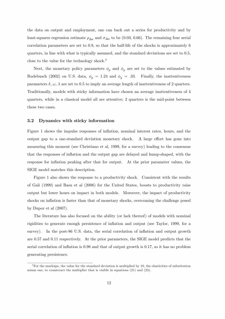
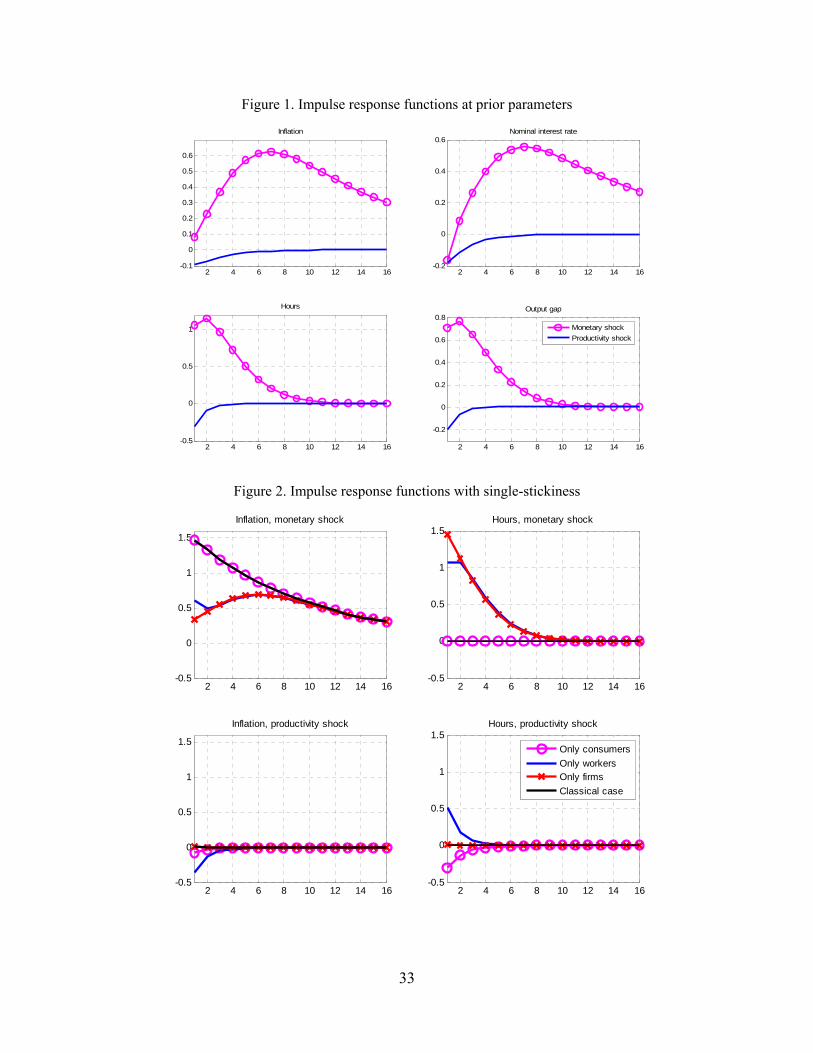
Figure 1 shows the impulse responses of in�ation, nominal interest rates, hours, and the

output gap to a one-standard deviation monetary shock. A large e¤ort has gone into

measuring this moment (see Christiano et al, 1999, for a survey) leading to the consensus

that the responses of in�ation and the output gap are delayed and hump-shaped, with the

response for in�ation peaking after that for output. At the prior parameter values, the

SIGE model matches this description.

Figure 1 also shows the response to a productivity shock. Consistent with the results

of Gali (1999) and Basu et al (2006) for the United States, boosts to productivity raise

output but lower hours on impact in both models. Moreover, the impact of productivity

shocks on in�ation is faster than that of monetary shocks, overcoming the challenge posed

by Dupor et al (2007).

The literature has also focused on the ability (or lack thereof) of models with nominal

rigidities to generate enough persistence of in�ation and output (see Taylor, 1999, for a

survey). In the post-86 U.S. data, the serial correlation of in�ation and output growth

are 0.57 and 0.11 respectively. At the prior parameters, the SIGE model predicts that the

serial correlation of in�ation is 0.98 and that of output growth is 0.17, so it has no problem

generating persistence.

4For the markups, the value for the standard deviation is multiplied by 10, the elasticities of substitutionminus one, to counteract the multiplier that is visible in equations (21) and (23).

12

A �nal empirical fact is the accelerationist Phillips curve, the positive correlation be-

tween the change in in�ation and the deviation of output from trend.5 The classical model

predicts that this moment is very close to zero, while in the U.S. data it is 0.29. The SIGE

model at the prior parameters predicts that the accelerationist Phillips curve correlation is

0.63.

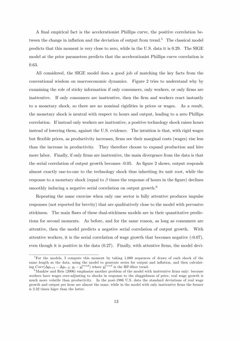
All considered, the SIGE model does a good job of matching the key facts from the

conventional wisdom on macroeconomic dynamics. Figure 2 tries to understand why by

examining the role of sticky information if only consumers, only workers, or only �rms are

inattentive. If only consumers are inattentive, then the �rm and workers react instantly

to a monetary shock, so there are no nominal rigidities in prices or wages. As a result,

the monetary shock is neutral with respect to hours and output, leading to a zero Phillips

correlation. If instead only workers are inattentive, a positive technology shock raises hours

instead of lowering them, against the U.S. evidence. The intuition is that, with rigid wages

but �exible prices, as productivity increases, �rms see their marginal costs (wages) rise less

than the increase in productivity. They therefore choose to expand production and hire

more labor. Finally, if only �rms are inattentive, the main divergence from the data is that

the serial correlation of output growth becomes -0.05. As �gure 2 shows, output responds

almost exactly one-to-one to the technology shock thus inheriting its unit root, while the

response to a monetary shock (equal to � times the response of hours in the �gure) declines

smoothly inducing a negative serial correlation on output growth.6

Repeating the same exercise when only one sector is fully attentive produces impulse

responses (not reported for brevity) that are qualitatively close to the model with pervasive

stickiness. The main �aws of these dual-stickiness models are in their quantitative predic-

tions for second moments. As before, and for the same reason, as long as consumers are

attentive, then the model predicts a negative serial correlation of output growth. With

attentive workers, it is the serial correlation of wage growth that becomes negative (-0.07),

even though it is positive in the data (0.27). Finally, with attentive �rms, the model devi-

5For the models, I compute this moment by taking 1,000 sequences of draws of each shock of thesame length as the data, using the model to generate series for output and in�ation, and then calculat-ing Corr(�pt+2 ��pt�2; yt � ytrendt ) where ytrendt is the HP-�lter trend.

6Mankiw and Reis (2006) emphasize another problem of the model with inattentive �rms only: becauseworkers have wages over-adjusting to shocks in response to the sluggishness of price, real wage growth ismuch more volatile than productivity. In the post-1986 U.S. data the standard deviations of real wagegrowth and output per hour are almost the same, while in the model with only inattentive �rms the formeris 2.32 times higer than the latter.

13

ates from the stylized facts in two ways: it predicts an increase in hours in response to an

improvement in productivity, and it predicts that real wage growth is more volatile than

productivity growth, when the opposite is true in the data.

To conclude, stickiness of information plays a role in all three markets in moving the

predictions of the model from their classical benchmark closer to the U.S. evidence. Inat-

tentiveness of �rms and workers setting prices and wages is required to have real e¤ects

of monetary shocks, and if only one of the two is inattentive, then real wages become too

volatile and technology shocks counterfactually raise hours. Inattentiveness of consumers

is required so there is positive serial correlation in the growth rates of consumption and

output, as is the case in the data.

3.3 Optimal policy rules

With the model and parameters picked there is a �laboratory� in place in which to ask

policy questions. To compare the performance of di¤erent policies, I focus on a utilitarian

measure of social welfare: the percentage increase in steady-state consumption under the

prior policy rule that would lead to the same unconditionally expected utility as in the

alternative policy being considered.

I focus on two policy rules that have dominated the literature. The �rst is the Taylor

(1993) rule:

it = �p�pt + �y(yt � yct ); (24)

with no monetary shocks, since in the SIGE model these lead to ine¢ cient �uctuations.

In reality, the policy shocks may be due to policy reacting to macroeconomic and �nancial

news other than in�ation and the output gap, or to the exercise of judgement and discretion,

or simply to policy mistakes, but in the model policy shocks are errors that unambiguously

lower welfare The second rule is a prive-level targeting rule:

pt = Kt � �(yt � yPOt ) (25)

that keeps the price level close to a deterministic target Kt, allowing for deviations in

response to deviations of output from its Pareto optimal level yPOt .7 In an economy with

7The Pareto-optimal output level di¤ers from the classical level yc as long as there are shocks to themarkups.

14

sticky information only on the side of �rms, Ball et al (2005) showed that this �elastic price

standard� is optimal. More generally, Svensson (2002) argued that a targeting rule like

this is superior to an instrument rule like the Taylor rule.

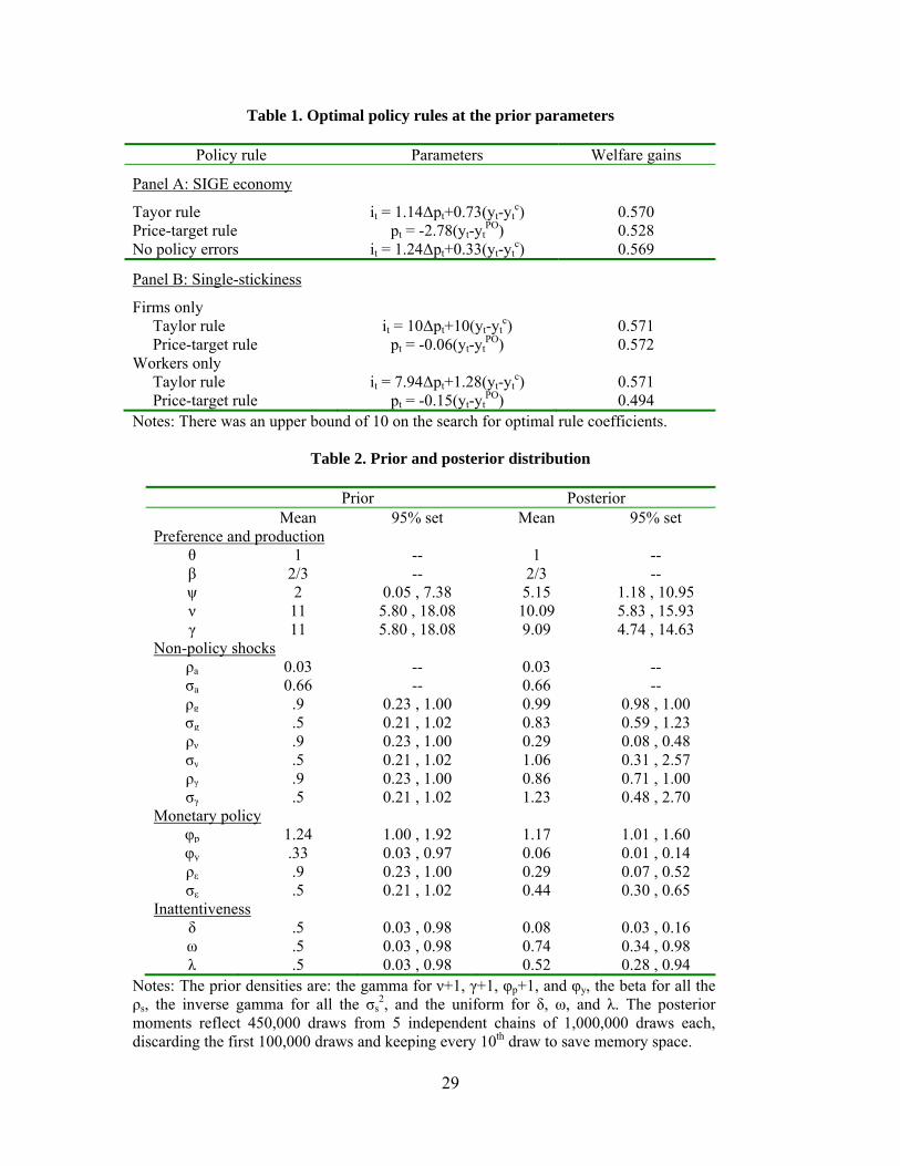
Table 1 shows the optimal rule coe¢ cients and welfare gains in the SIGE economy.

Both rules respond strongly to output deviations; in particular, the optimal �y is 2.2 times

higher than its prior value. This reveals an important feature of SIGE economies that holds

for many parameter values: �uctuations in real activity are considerably more costly than

�uctuations in in�ation, so policy is particularly concerned with real stabilization. Both

rules reach signi�cant welfare gains, most of which come from eliminating the ine¢ cient

monetary policy shocks, as shown in the third row.

To understand better what drives optimal policy in the SIGE model, panel B in table

1 shows the optimal policy coe¢ cients and welfare gains if there is sticky information in

only one market. If only consumers are inattentive, there are no nominal rigidities since

they choose real consumption. Monetary policy is neutral, so any monetary policy rule is

as good as another.

If only �rms are inattentive, we are in the setup considered by Ball et al (2005), in

which case the price-level target dominates the Taylor rule. Intuitively, keeping the price

level on target reduces the mistakes that �rms make with their price plans due to outdated

information. However, in response to temporary shocks to markups inducing ine¢ cient

�uctuations in real quantities, it is best to let prices deviate from the target so as to

attenuate the real �uctuations. The Taylor rule, because it responds to in�ation, creates

base drift in the price level, so the price-setters with information older than the shock

continue making incorrect forecasts of prices into the future. Being constrained to follow a

Taylor rule, policy reacts very strongly to the output gap, since this reduces the extent of

base drift and comes closer to the optimal price-level targeting rule.

If only workers are inattentive, the Taylor rule performs better. The reason is that, while

workers have to forecast the price-level to set their plans for wages, they also have to forecast

in�ation (via the long-run interest rate) in order to assess how much to intertemporally

substitute their supply of labor. Targeting in�ation, at least partially, becomes legitimate

and the Taylor rule performs as well as the price-level target.

15

4 Application the United States

The previous section characterized macro-dynamics and optimal policy in the SIGE model

for a particular choice of parameters based on prior information. This section uses the

U.S. data to choose a new set of parameters and updates the conclusions on dynamics and

policy for this empirically realistic case.

4.1 Comparing model and data using estimates

Starting from the prior parameters from other studies that were used in the previous section,

I take a Bayesian approach to combine them with data taking uncertainty into account.

Given the data Y, this consists of assigning prior uncertainty to the parameters in the

previous section via a joint probability density p(�), assuming that the �ve shocks are

independently normally distributed to derive the likelihood function L(Y j �), and then

obtaining the posterior density for the parameters p(� j Y). This is done numerically,

using Markov Chain Monte Carlo simulations.8

The prior density p(�) follows the convention in the DSGE literature (e.g., An and

Schorfheide, 2007) for most parameters. The �rst section of table 2 displays the choices.

Each parameter is treated independently, and is assigned a particular distribution with a

mean equal to the choices in the previous section, and a relatively large variance. The prior

for the adjustment parameters is �at in the unit interval.

The second section of table 2 shows the posterior parameter estimates. Starting with

the preference and production parameters, the elasticities of substitution across varieties

are roughly similar to the priors. The elasticity of labor supply however, is more than twice

as large as the prior, and even though the 95% credible set is wide, all values in it are quite

large. Such an elastic labor supply is consistent with the typical assumption in business

cycle models, but it goes against estimates using microeconomic data.9 Another parameter

where there is a large di¤erence between priors and posterior means is the response of

nominal interest rates to real activity, which is considerably lower in the estimates than in

the prior assumptions. The estimates of the persistence of monetary policy shocks is also

8A companion paper, Reis (2008), describes the simulation procedure in more detail and examines thesensitivity of the results to di¤erent prior speci�cations.

9Rogerson and Wallenius (2007) provide a recent re-statement of the disparity between micro and macroelasticities, and propose a resolution.

16

lower than in the prior, with only 29% of a shock remaining after one period.

Turning to the more interesting inattentiveness parameters, �rms are estimated to on av-

erage be inattentive for 6 months, workers for 4 months, and consumers for 36 months. The

fact that consumers are very inattentive is not too shocking, since as Reis (2006) showed,

a consumer that is inattentive forever would optimally choose to live hand-to-mouth, con-

suming his income every period, and between 20% and 50% of the U.S. population seems to

live this way.10 More puzzling is the discrepancy between consumers and workers. Broadly

interpreted, these estimates point to U.S. wages being quicker to adjust to news than U.S.

consumption choices. Narrowly interpreted, they imply that workers are more attentive

than consumers, which may be understandable in the light of two facts: �rst, the probability

that an employment relationship is terminated every month is on average 3%, and second,

the wage series used in the estimation was total compensation, of which 1/4 is non-wage

payments and includes bonuses.11 Whether because employment spells are on average

relatively short, or because there are many margins of compensation that may change at

high frequencies, there is some justi�cation for U.S. workers to pay frequent attention to

their compensation.

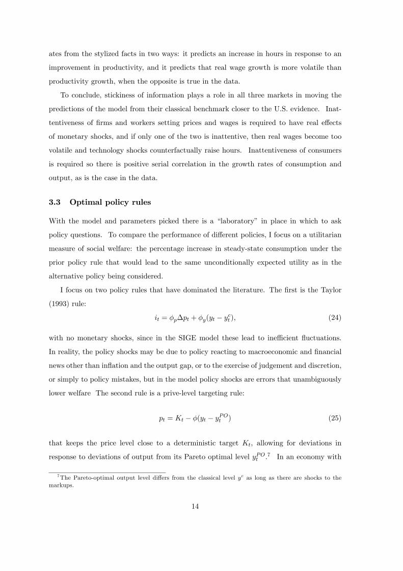
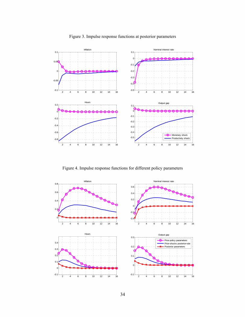
Figure 3 shows the impulse responses to monetary and productivity shocks at the mean

posterior parameters. The response to productivity shocks is larger and faster than at the

priors, but qualitatively the shapes are similar. In response to monetary shocks though,

all variables move faster than at the prior parameters, without any hump shapes. This

fast reaction of macroeconomic variables to policy shocks is consistent with the �ndings of

Boivin and Giannoni (2006). They note that while much of the evidence for delayed and

hump-shaped responses to monetary policy shocks comes from looking at the U.S. post-

war, in the United States post the mid-1980s, the impact of monetary shocks has become

much faster according to VARs. The source of the prior used for �gure 1 comes from

studies looking at post-war data, whereas the posteriors in �gure 3 use data post-1988.

The contrast between these two �gures is in line with the VAR evidence.

To understand what is driving it in the SIGE model, �gure 4 shows the same impulse re-

sponse for three sets of parameters. Across all sets, the non-policy parameters are the same

and equal to the mean of the posterior distribution. They di¤er in the policy parameters,

10See Campbell and Mankiw (1989), Hurst (2006), Reis (2006a) and the references therein.11See Hall (2006) and Pierce (2001).

17

as in one case, both policy-rule parameters (�p and �y) and policy-shock parameters (�";

�") are kept at the prior parameter values, in the second case the policy-rule parameters are

updated but the policy-shock parameters are not, and in the third case all parameters are

at the mean posterior (as in �gure 3). Figure 4 makes clear that the qualitative di¤erences

between the dynamics at the prior and posterior are not due to a di¤erence in the monetary

transmission mechanism. Rather, monetary policy has quick e¤ects with no hump-shapes

at the posterior exclusively because the persistence of the shocks is much smaller at the

posterior than at the prior.12

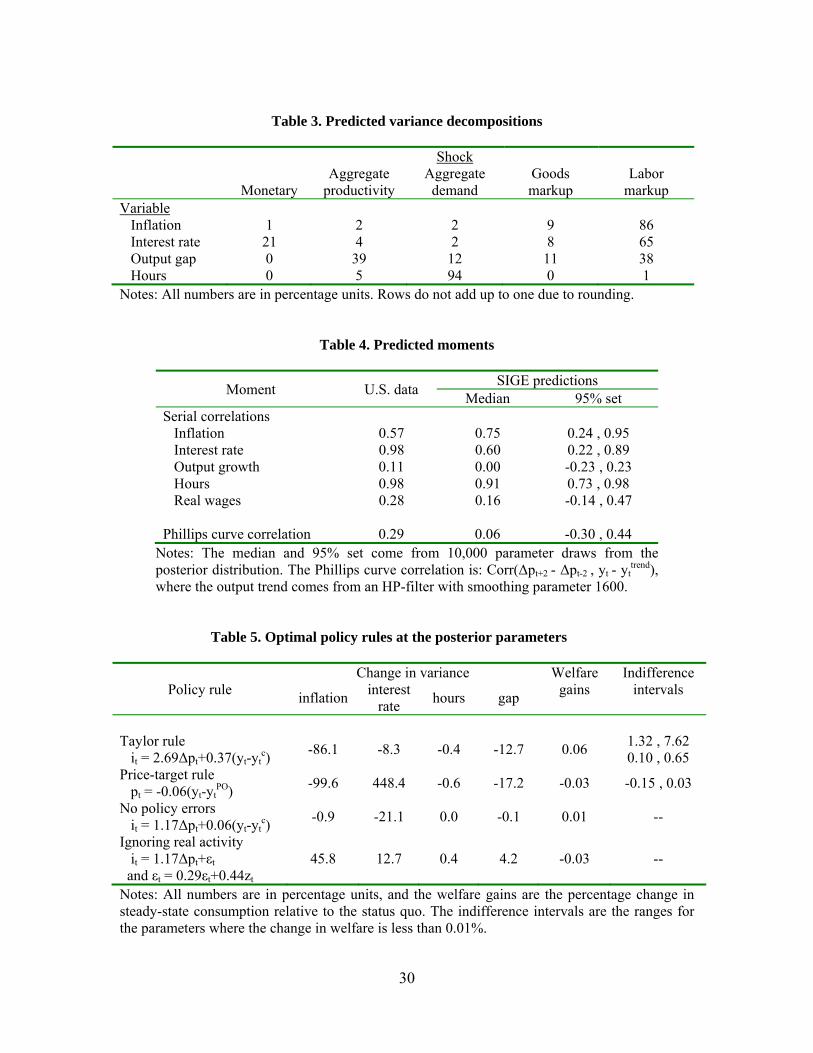
Table 3 has the predicted variance decompositions at an in�nite horizon. Using VARs,

Christiano et al (1999) and Bernanke et al (2005) �nd that monetary policy shocks in the

United States play a small role in all variables except the nominal interest rate. The SIGE

model is consistent with these predictions. Productivity shocks play a signi�cant role for the

U.S. output gap, while aggregate demand shocks are important especially to explain hours.

Finally, wage-markup shocks are quite important, while price-markup shocks are less so.

Table 4 shows the predicted serial correlations and Phillips correlation. As expected,

taking the data and uncertainty into account move the predictions closer to the data,

although taking the uncertainty in the parameters into account, the model�s predictions

are imprecisely estimated.

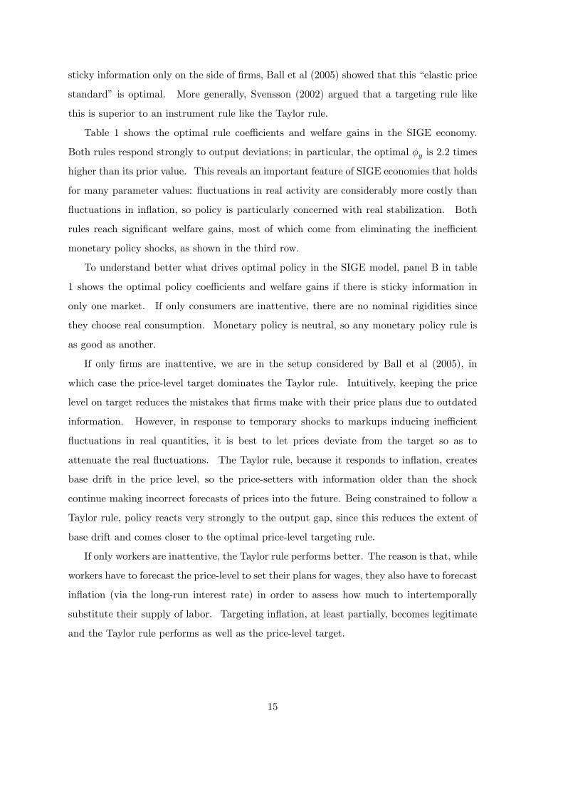
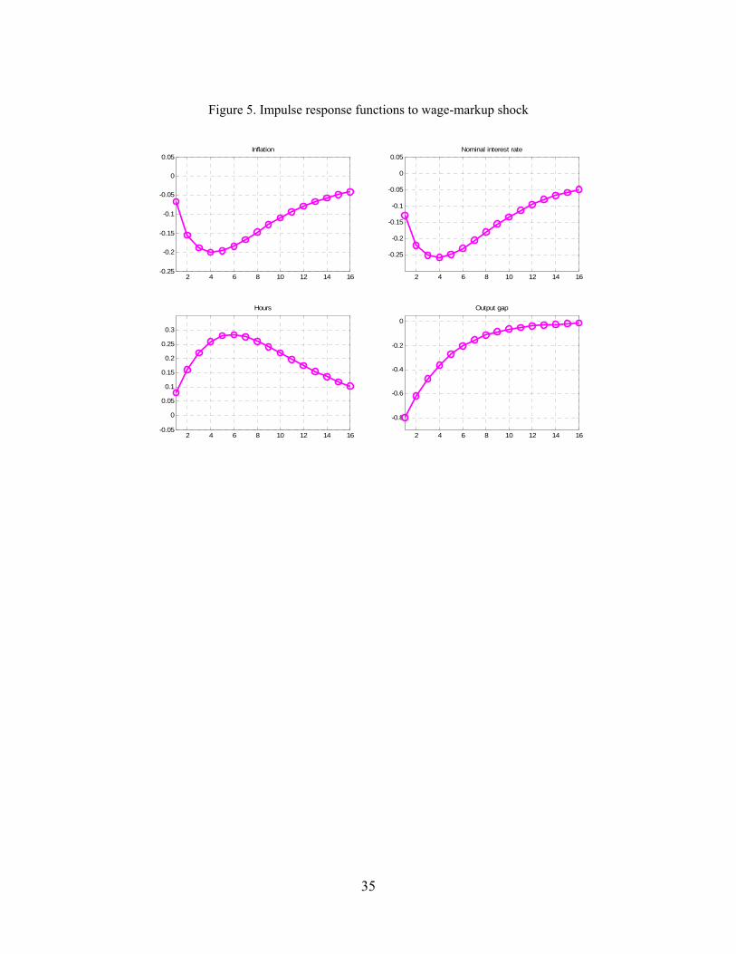
Because wage-markup shocks are so important, �gure 5 plots the impulse response to

them at the posterior parameters. A positive shock corresponds to a fall in the desired

markup. Hours therefore rise as wages fall, but because of inattention, �rms do not expand

production by as much as they would with full information, so that a negative output gap

results. The fall in wages induces a fall in prices, so in�ation falls. Noticeably, the responses

of in�ation and hours are both hump-shaped and delayed. This is particularly important

because it largely explains why the model is able to match the Phillips correlation. In

response to these shocks (that explain a large part of the variance of in�ation and the

output gap), for the �rst few periods, the change in in�ation is negative, while the output

gap is large and negative, so the correlation between the two is positive.

12Coibion (2006) also �nds a large role of the persistence of monetary shocks on their impact on in�ationand output in a simpler sticky-information model.

18

4.2 The optimal Taylor and price-targeting rules

Table 5 shows the Taylor rule that maximizes social welfare, as well as its impact on the

variance of a few variables, and �indi¤erence intervals�calculated as the range within which

each parameter can change without changing welfare by more than 1 basis point. Noticeably,

policy optimally responds by more to in�ation than in the status quo. Moreover, the

indi¤erence intervals for �p are asymmetric, showing that as long as the response to in�ation

is su¢ ciently large, the exact value of �p is not very important for welfare. According to

SIGE, policy should be quite sensitive to the output gap and the welfare bene�ts from this

rule relative to the status quo would be 6 bp.

To understand better these results, note that contrary to the case at the prior parame-

ters, eliminating policy errors has a negligible impact on variability and welfare. This is

due to the small estimate for the volatility of monetary policy shocks in the U.S. economy

since 1986, and it is the reason why the welfare gains are smaller in table 5 than they were

in table 1. Moreover, table 5 shows again that stabilization policy is very valuable in the

SIGE model. Even though the estimated �y was small, setting it equal to zero produces a

large increase in volatility and signi�cantly lower welfare

Turning to the optimal elastic price-level standard, it is essentially inelastic. The rule

performs quite well from the perspective of stabilizing the output gap and in�ation, but in

terms of social welfare it does not improve over the status quo. Because in the estimates,

price-setters are more inattentive than wage-setters, this rule is close to the one that we

calculated earlier for an economy with only inattentive �rms.

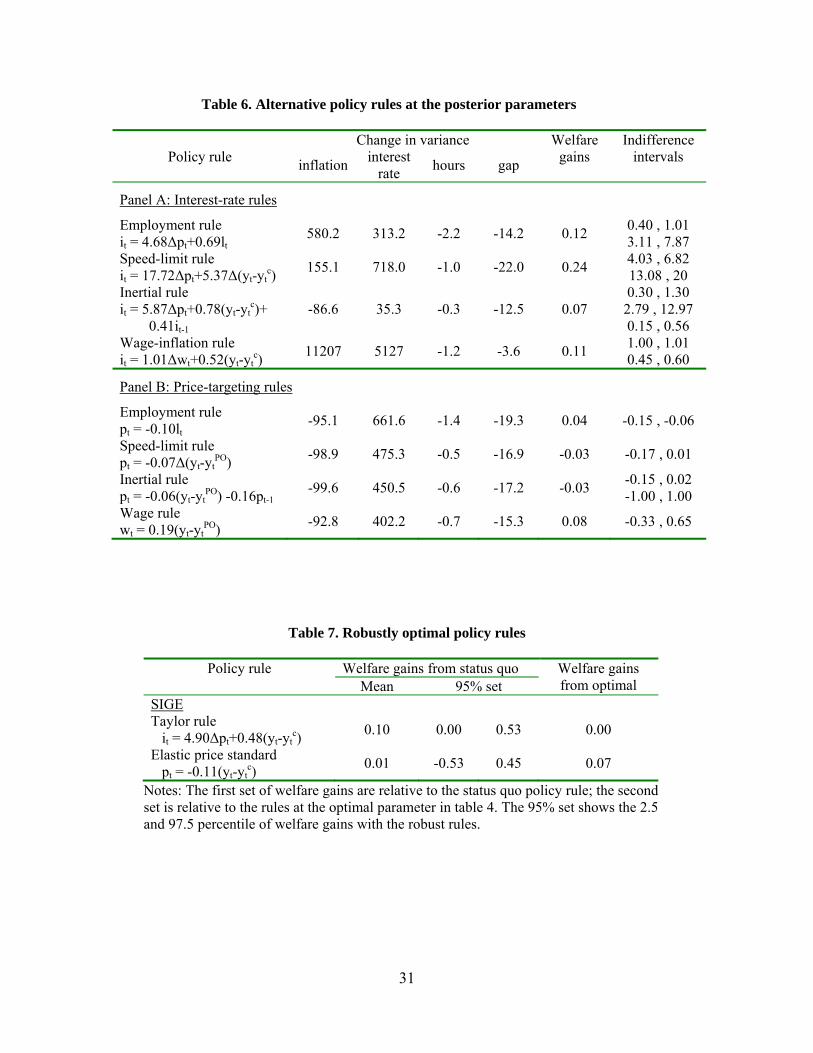
4.3 Alternative rules

Over the past decade, a variety of di¤erent interest-rate rules have been proposed as an

alternative to Taylor�s suggestion. Orphanides (2003) noted that the output gap is hard to

estimate in real time and mistakes about its value can lead policy astray. An alternative

interest-rate rule that safeguards against this danger might respond instead to hours worked

as the measure of real activity. Orphanides and Williams (2002) and Walsh (2003) instead

argued in favor of replacing the level of the output gap with its growth rate in the Taylor

rule. Table 6 shows that these policy rules do quite well in terms of welfare, although this

comes at the expense of a large increase in the volatility for nominal variables.

19

Woodford (2003) noted that sticky-price models provide a reason for interest-rate inertia

as a form of policy commitment inducing �rms to adjust their prices faster to shocks today.

In the SIGE model, because �rms can set future prices di¤erent from current prices in their

plans, this motive is absent so the welfare bene�ts from inertia are insigni�cant. Table

6 shows also that responding to wage rater than price in�ation, as argued in Erceg et al

(2000), leads to extremely volatile price-in�ation and nominal interest rates, in return for a

modest reduction in the volatility of hours and the output gap. As a result, it does worse

than either the employment or speed-limit rules.

Table 6 also looks at modi�cations of the price-level targeting rule that mimic these

modi�cations of the Taylor rule. The best performing rule is an elastic wage-level target,

in which wages are allowed to rise above target in a boom. In response to a shock that

leads to a positive output gap, the policymaker wants to induce a disin�ation to contract the

economy. However, if �rms are more attentive than workers (as in the case of the United

States), then by committing to raise nominal wages in response to a shock, the policymaker

ensures that real wages rise, inducing �rms to cut production and stabilize real activity.

5 Robustness of the conclusions

I inspect the robustness of the conclusions to the parameters in two ways: by computing

robustly-optimal policy rules for the United States, and by repeating the analysis for a

di¤erent but similar economy, the Euro-area post-Maastricht.

5.1 Robustness to parameter uncertainty

The calculations so far evaluated optimal welfare at the mean parameter estimates. Split-

ting the parameter vector � into two vectors, one with the policy parameters �p and another

with the non-policy parameters �np, and writing the unconditional expectations of social

welfare as W(�p;�np), the optimal policy rules chose �p to maximize:

W��p;

Z�npdp(�npjYt)

�; (26)

where p(�npjYt) was the posterior distribution.

By taking the parameters at their mean, this approach ignores the uncertainty in the

estimates. One approach to take it into account is to focus instead on maximizing integrated

20

social welfare: ZW(�p;�np)dp(�npjYt): (27)

Levin et al. (2006) and Edge at al. (2007) call the policies that maximize this criteria

�robustly� optimal in the sense that they are the best after averaging over the di¤erent

models that correspond to each �np, and Sims (2001) defends this Bayesian model-averaging

as an alternative to �min-max�analysis.

Table 7 shows the robustly-optimal Taylor rules and elastic price-level standards ac-

cording to integrated welfare.13 The Taylor rules are more aggressive in their response

to in�ation and output, and the price-level standards are more elastic.14 Relative to the

status quo, the robustly-optimal Taylor rule performs quite well both on average as well as

in most circumstances, since more than 95% of the times it leads to outcomes no worse than

the current ones. Compared instead to the optimal Taylor rule that ignored parameter

uncertainty, the bene�ts from taking robustness into account are small.

Turning to the elastic price-targeting rules, they are more elastic when uncertainty is

taken into account, and the gains in welfare are 7 bp. However, there is a sense in which

this price-level standard is not very robust: more than 5% of the times it leads to welfare

losses of half a percentage point in consumption units.

Comparing the two types of rules more directly, the Taylor rule performs better than

the elastic price standard 82% of the times in the United States. Moreover, while the worst

scenarios under the robust policy rule lead to welfare losses of 10 bp, under the robust

price-level standard, for some parameter values, the welfare losses can be as high as 90 bp.

Thus, while �robustness�in this section was interpreted as model-averaging, a �min-max�

perspective would also lead to preferring interest-rate rules over price-targeting rules.

5.2 Are the conclusions for the Euro-area di¤erent?

The Euro-area post Maastricht treaty (1993:4�2005:4) is the closest region in the world to

the United states post-1986 in terms of size, structure of the economy, and monetary-policy

regime. Checking whether the policy conclusions for this area agree with those for the

13To �nd these optima, I averaged over 10,000 draws from the posterior density to approximate theintegral, and maximised over sequence of grids, with jumps of size 1, 0.1, and 0.01.14Taking a min-max perspective in a sticky-price model, Giannoni (2007) �nds also that a concern for

robustness lads to more responsive interest-rate responses.

21

United States provides an alternative check on their robustness.

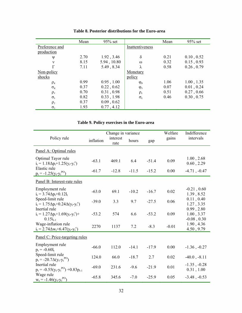
Table 8 shows the posterior parameters from performing the same estimation exercise

using the Euro-area data. Most estimates are relatively similar to those for the United

States, including the policy rule and the inattentiveness of European �rms. The main

exception is the inattentiveness of workers and consumers. In Europe, consumers update

their information on average every 15 months, while workers do so every 9 months, and

the two 95% credible sets has a large overlapping range. The Euro-area data is consistent

with the two members of the household updating at the same time so that consumption

and wage-setting decisions are made in tandem.15

Table 9 provides the counterpart to tables 5 and 6 for the Euro-area. Most of the

conclusions on the desirability of di¤erent rules hold up for the Euro-area, with three sig-

ni�cant exceptions. First, the welfare bene�ts of moving policy from the status quo to

optimal alternatives are usually about twice larger for the Euro-area than for the United

States. While I cannot be sure of what exactly drives this di¤erence, altering the Euro-area

parameters one-by-one to match the U.S. parameters gives a clue. Much of the di¤erence

in the size of welfare bene�ts seems to be due to the elasticity of labor supply being

half as large in the Euro-area as in the United States, so that �uctuations in real variables

and hours worked more generally have a higher welfare cost. Second, the optimal Taylor

rule in panel A dominates all of the interest-rate rules in panel B. Third, while elastic

wage-targeting is also the best targeting policy for the Euro-area, the sign of the coe¢ cient

is the opposite of that for the United States. This discrepancy is likely due to the di¤erence

in the relative inattentiveness of workers vis-a-vis �rms in the two economies. Unlike in

the United States, in the Euro-area, workers are more attentive than �rms. Therefore,

by committing to induce a fall in nominal wages, the policymaker encourages the attentive

workers to cut hours worked and through this channel the production of the inattentive

�rms.

15Curiously, Mankiw and Reis (2007) found this was also the case for the post-war U.S. data. Thediscrepancy between workers and consumers�inattentiveness seems to be speci�c to the recent U.S. data.

22

6 Relation to optimal policy with sticky actions

There is a large literature studying optimal monetary policy in new Keynesian general

equilibrium models (see Gali, 2008 for a selective survey). The adequate comparison group

for the results in this paper is formed by studies of monetary policy in models that account

for at least the dynamics of 3 variables, and that were estimated to �t the U.S. data. In this

group, there are three main studies, all of which use variants of the Christiano et al (2005)

model. This model assumes that there are costs of adjusting actions, not information, so

that agents choose plans that are not only based on outdated information but must also be

constant over time. At the same time, in this model, a series of indexation clauses allow

actions to respond (albeit mechanically) to current news.

Schmitt-Grohe and Uribe (2007) calculate the optimal coe¢ cients in an inertial interest-

rate rule that responds to in�ation, wage growth, and output growth. Consistent with the

results for the SIGE model, they �nd that interest-rate inertia is modest and has a small

impact on welfare, that optimal policy is quite aggressive in its response to in�ation, and

that is more important to focus on wage rather than price in�ation. Unlike the results for

the SIGE model though, they �nd that it is best for interest rates to not respond to any

measure of real activity.

In turn, Juillard et al (2006) �nd that optimal policy tends to generate quite volatile

in�ation and nominal interest rates, similar to what was found in this paper. However, the

volatility of in�ation that is tolerable with little impact on welfare is much higher here than

in their work.

Finally, Levin et al (2007) �nd that a simple rule that focus solely on wage in�ation

performs very well and is quite robust to parameter uncertainty. The surprising robustness

of optimized interest-rate rules to parameter uncertainty is also true in the SIGE model,

although I found that this is less true of targeting rules. The SIGE model also con�rms a

desire to focus on wage in�ation, although taking into account real activity is very important

here but not in their work.

Combining the comparisons with these three papers, it seems that in models with sticky

information, in�ation is not as much of a policy concern as in sticky-actions models. In

SIGE, optimal policy is more responsive to measures of real activity and more tolerant of

in�ation volatility. While this di¤erence has many roots, a key one is perhaps that �rms

23

and workers that set time-varying plans for prices and wages can more �exibly accommodate

to in�ation than agents constrained to set the same price and wage over time.

7 Policy conclusions

Starting from a baseline model that is similar to the core of many DSGE monetary models

and from conventional prior parameter choices, this paper introduced rigidities by assuming

sticky information instead of the more popular assumption of sticky actions. It then

performed a series of counterfactual policy experiments that, while probably infeasible in

the real world, could be analyzed within the arti�cial world that the SIGE model provides.

These experiments led to a few concrete lessons for applied monetary policy:

1. interest rates should respond more aggressively to in�ation than they have;

2. it is important for interest rates to respond to measures of real activity, even though

the best measure of it may be the output gap, the level of employment, or the change

in the output gap;

3. targeting rules typically perform worse than interest-rate rules, and the optimal target

is on wage-in�ation;

4. optimal interest rate rules are quite robust to parameter uncertainty, while targeting

rules are less so, and a concern for robustness leads to more aggressive policy rules.

Compared with the literature on sticky actions, the �rst lesson is shared, but the second

is not. (That literature has not studied targeting rules so there is no counterpart to the

other two lessons.) In general and across several policy experiments, sticky-information

models seem to put a larger emphasis on real stabilization versus in�ation stabilization

relative to sticky-action models and in particular, often imply quite volatile in�ation.

Finally, note that the optimal policy rules typically led to gains of around 0.10% of

steady-state consumption. In the United States in 2006 this would be worth $9,240 millions.

By comparison, recent conservative estimates of the costs of �uctuations put them around

0.5-1%, so that better monetary policy could eliminate somewhere between one tenth and

one-quarter of the welfare costs of business cycles, not a small deal.16 Another relevant

16See Alvarez and Jermann (2004) and Reis (forthcoming) for recent estimates of the costs of �uctuations.

24

comparison is with the total expenses of the Federal Reserve Banks, which were $3,264

millions in 2006. If the scope for improving monetary policy can reach gains that are

almost three times as large as the budget of the central bank, this is a tempting area for

policy improvement.

References

Akerlof, George A. and Janet L. Yellen (1985). �A Near-Rational Model of the Business

Cycle, with Wage and Price Inertia.�Quarterly Journal of Economics, vol. 100, pp.

823-838.

Alvarez, Fernando and Urban J. Jermann (2004). �Using Asset Prices to Measure the Cost

of Business Cycles.�Journal of Political Economy, vol. 112 (6), pp. 1223-1256.

An, Sungbae and Frank Schorfheide (2007). �Bayesian Analysis of DSGE Models.�Econo-

metric Reviews, vol. 26 (2-4), pp. 113-172.

Ball, Laurence, N. Gregory Mankiw, and Ricardo Reis (2005). �Monetary Policy for Inat-

tentive Economies.�Journal of Monetary Economics, vol. 52 (4), pp. 703-725.

Basu, Susanto and John G. Fernald (1997). �Returns to Scale in U.S. Production: Estimates

and Implications.�Journal of Political Economy, vol. 105 (2), pp. 249-283.

Basu, Susanto, John G. Fernald, and Miles S. Kimball (2006). �Are Technology Improve-

ments Contractionary?�American Economic Review, vol. 96 (5), pp. 1418-48.

Bernanke, Ben, Jean Boivin and Piotr S. Eliasz (2005). �Measuring the E¤ects of Monetary

Policy: A Factor-augmented Vector Autoregressive (FAVAR) Approach.�Quarterly

Journal of Economics, vol. 120 (1), pp. 387-422.

Blanchard, Olivier and John Simon (2001). �The Long and Large Decline in U.S. Output

Volatility.�Brookings Papers on Economic Activity, vol. 1, pp. 135-64.

Boivin, Jean and Marc Giannoni (2006). �Has Monetary Policy Become More E¤ective?�

Review of Economics and Statistics, vol. 88 (3), pp. 445-462.

Campbell, John Y. and N. Gregory Mankiw (1989). �Consumption, Income and Interest

Rates: Reinterpreting the Time Series Evidence.�NBER Macroeconomics Annual,

vol. 4, pp. 185-216.

Christiano, Lawrence J., Martin Eichenbaum, and Charles L. Evans (1999). �Monetary

Policy Shocks: What Have We Learned and to What End?� in Handbook of Macro-

economics, edited by John Taylor and Michael Woodford, Elsevier.

25

Christiano, Lawrence J., Martin Eichenbaum, and Charles L. Evans (2005). �Nominal

Rigidities and the Dynamic E¤ects of an Shock to Monetary Policy.� Journal of

Political Economy, vol. 113 (1), pp. 1-45.

Coibion, Olivier (2006). �In�ation Inertia in Sticky Information Models.�B.E. Journals

Contributions to Macroeconomics, vol. 6 (1).

Dupor, Bill, Jing Han, and Yi Chan Tsai (2007). �What do Technology Shocks Tells Us

about the New Keynesian Paradigm?�Unpublished manuscript.

Edge, Rochelle M., Thomas Laubach, and John C. Williams (2007). �Welfare-Maximizing

Monetary Policy under Parameter Uncertainty.�Finance and Economics Discussion

Series 2007-56.

Erceg, Christopher, Dale Henderson and Andrew Levin (2000). �Optimal Monetary Policy

with Staggered Wage and Price Contracts.�Journal of Monetary Economics, vol. 46,

pp. 281-313.

Gali, Jordi (1999). �Technology, Employment, and the Business Cycle: Do Technology

Shocks Explain Aggregate Fluctuations?�American Economic Review, vol. 89 (1),

pp. 249-271.

Gali, Jordi (2008). Monetary Policy, In�ation, and the Business Cycle. MIT Press: Cam-

bridge, USA.

Giannoni, Marc (2007). �Robust Optimal Monetary Policy in a Forward-Looking Model

with Parameter and Shock Uncertainty.�Journal of Applied Economics, vol. 22 (1),

pp. 179-213.

Hall, Robert E. (2006). �Job Loss, Job Finding, and Unemployment in the U.S. Economy

over the Past Fifty Years.�NBER Macroeconomics Annual, vol. 20, pp. 101-137.

Hurst, Erik (2006). �Grasshoppers, Ants, and Pre-Retirement Wealth: A Test of Permanent

Income consumers.�NBER Working Paper 10,098.

Juillard, Michel, Philippe Karam, Douglas Laxton, and Paolo Pesenti (2006). �Welfare-

Based Monetary Policy Rules in an Estimated DSGE Model of the U.S. Economy�

European Central Bank Working Paper 613.

Levin, Andrew T., Alexei Onatski, John C. Williams and Noah Williams (2006). �Monetary

Policy Under Uncertainty in Micro-Founded Macroeconometric Models.� In NBER

Macroeconomics Annual 2005, edited by Mark Gertler and Kenneth Rogo¤, MIT

Press: Cambridge.

26

Mankiw, N. Gregory and Ricardo Reis (2002). �Sticky Information versus Sticky Prices:

A Proposal to Replace the New Keynesian Phillips Curve.� Quarterly Journal of

Economics, 117 (4), 1295-1328.

Mankiw, N. Gregory and Ricardo Reis (2006). �Pervasive Stickiness.�American Economic

Review, vol. 96 (2), pp. 164-169.

Mankiw, N. Gregory and Ricardo Reis (2007). �Sticky Information in General Equilibrium.�

Journal of the European Economic Association, vol. 2 (2-3), pp. 603-613.

Orphanides, Athanasios (2003). �The Quest for Prosperity Without In�ation.�Journal of

Monetary Economics, vol. 50 (3), pp. 633-663.

Orphanides, Athanasios and John C. Williams (2002). �Robust Monetary Policy Rules

with Unknown Natural Rates.�Brookings Papers on Economic Activity, vol. 2, pp.

63-118.

Pierce, Brooks (2001). �Compensation Inequality.�Quarterly Journal of Economics, vol.

116 (4), pp. 1493-525.

Reis, Ricardo (2006a). �Inattentive Consumers,�Journal of Monetary Economics, vol. 53

(8), pp. 1761-1800.

Reis, Ricardo (2006b). �Inattentive Producers,�Review of Economic Studies, vol. 73 (3),

pp. 793-821.

Reis, Ricardo (2007). �The Time-Series Properties of Aggregate Consumption: Implica-

tions for the Costs of Fluctuations.�Journal of the European Economic Association,

forthcoming.

Reis, Ricardo (2008). �A Sticky-Information General Equilibrium Model for Policy Analy-

sis.�Unpublished manuscript.

Rogerson, Richard and Johanna Wallenius (2007). �Micro and Macro Elasticities in a Life

Cycle Model with Taxes.�NBER working paper 13,017.

Rudebusch, Glenn D. (2002). �Term Structure Evidence on Interest Rate Smoothing and

Monetary Policy Inertia.�Journal of Monetary Economics, vol. 49 (6), pp. 1161-1187.

Schmitt-Grohe, Stephanie and Martin Uribe (2007). �Optimal In�ation Stabilization in a

Medium-Scale Macroeconomic Model.�InMonetary Policy Under In�ation Targeting,

edited by Klaus Schmidt-Hebbel and Rick Mishkin, Central Bank of Chile: Santiago,

Chile.

Sims, Christopher A. (2001). �Pitfalls of a Minimax Approach to Model Uncertainty.�

27

American Economic Review, vol. 91 (2), pp. 51-54.

Smets, Frank and Rafael Wouters (2003). �An Estimated Stochastic Dynamic General

Equilibrium Model of the Euro Area.�Journal of the European Economic Association,

vol. 1 (5), pp. 1123�1175.

Svensson, Lars E. O. (2003). �What Is Wrong with Taylor Rules? Using Judgment in

Monetary Policy through Targeting Rules.�Journal of Economic Literature, vol. 41,

pp. 426-477.

Taylor, John B. (1979). �Estimation and Control of a Macroeconomic Model with Rational

Expectations.�Econometrica, vol. 47 (5), pp. 1267�1286.

Taylor, John B. (1999). �Staggered Price and Wage Setting in Macroeconomics.�in Hand-

book of Macroeconomics, edited by John Taylor and Michael Woodford, Elsevier.

Walsh, Carl E. (2003). �Speed Limit Policies: The Output Gap and Optimal Monetary

Policy.�American Economic Review, vol. 93 (1), pp. 265-278.

Woodford, Michael (2003). �Optimal Interest-Rate Smoothing.�Review of Economic Stud-

ies, vol. 70, pp. 861-886.

28

29

Table 1. Optimal policy rules at the prior parameters

Policy rule Parameters Welfare gains

Panel A: SIGE economy

Tayor rule it = 1.14Δpt+0.73(yt-yt

c) 0.570 Price-target rule pt = -2.78(yt-yt

PO) 0.528 No policy errors it = 1.24Δpt+0.33(yt-yt

c) 0.569

Panel B: Single-stickiness

Firms only Taylor rule it = 10Δpt+10(yt-yt

c) 0.571 Price-target rule pt = -0.06(yt-yt

PO) 0.572 Workers only Taylor rule it = 7.94Δpt+1.28(yt-yt

c) 0.571 Price-target rule pt = -0.15(yt-yt

PO) 0.494 Notes: There was an upper bound of 10 on the search for optimal rule coefficients.

Table 2. Prior and posterior distribution

Prior Posterior Mean 95% set Mean 95% set

Preference and production θ 1 -- 1 -- β 2/3 -- 2/3 -- ψ 2 0.05 , 7.38 5.15 1.18 , 10.95 ν 11 5.80 , 18.08 10.09 5.83 , 15.93 γ 11 5.80 , 18.08 9.09 4.74 , 14.63

Non-policy shocks ρa 0.03 -- 0.03 -- σa 0.66 -- 0.66 -- ρg .9 0.23 , 1.00 0.99 0.98 , 1.00 σg .5 0.21 , 1.02 0.83 0.59 , 1.23 ρν .9 0.23 , 1.00 0.29 0.08 , 0.48 σν .5 0.21 , 1.02 1.06 0.31 , 2.57 ργ .9 0.23 , 1.00 0.86 0.71 , 1.00 σγ .5 0.21 , 1.02 1.23 0.48 , 2.70

Monetary policy φp 1.24 1.00 , 1.92 1.17 1.01 , 1.60 φy .33 0.03 , 0.97 0.06 0.01 , 0.14 ρε .9 0.23 , 1.00 0.29 0.07 , 0.52 σε .5 0.21 , 1.02 0.44 0.30 , 0.65

Inattentiveness δ .5 0.03 , 0.98 0.08 0.03 , 0.16 ω .5 0.03 , 0.98 0.74 0.34 , 0.98 λ .5 0.03 , 0.98 0.52 0.28 , 0.94

Notes: The prior densities are: the gamma for ν+1, γ+1, φp+1, and φy, the beta for all the ρs, the inverse gamma for all the σs

2, and the uniform for δ, ω, and λ. The posterior moments reflect 450,000 draws from 5 independent chains of 1,000,000 draws each, discarding the first 100,000 draws and keeping every 10th draw to save memory space.

30

Table 3. Predicted variance decompositions

Shock

Monetary Aggregate

productivity Aggregate

demand Goods markup

Labor markup

Variable Inflation 1 2 2 9 86 Interest rate 21 4 2 8 65 Output gap 0 39 12 11 38 Hours 0 5 94 0 1 Notes: All numbers are in percentage units. Rows do not add up to one due to rounding.

Table 4. Predicted moments

Moment U.S. data SIGE predictions

Median 95% set Serial correlations Inflation 0.57 0.75 0.24 , 0.95 Interest rate 0.98 0.60 0.22 , 0.89 Output growth 0.11 0.00 -0.23 , 0.23 Hours 0.98 0.91 0.73 , 0.98 Real wages 0.28 0.16 -0.14 , 0.47 Phillips curve correlation 0.29 0.06 -0.30 , 0.44

Notes: The median and 95% set come from 10,000 parameter draws from the posterior distribution. The Phillips curve correlation is: Corr(Δpt+2 - Δpt-2 , yt - yt

trend), where the output trend comes from an HP-filter with smoothing parameter 1600.

Table 5. Optimal policy rules at the posterior parameters

Change in variance Welfare Indifference Policy rule

inflation interest

rate hours gap

gains intervals

Taylor rule it = 2.69Δpt+0.37(yt-yt

c) -86.1 -8.3 -0.4 -12.7 0.06

1.32 , 7.62 0.10 , 0.65

Price-target rule pt = -0.06(yt-yt

PO) -99.6 448.4 -0.6 -17.2 -0.03 -0.15 , 0.03

No policy errors it = 1.17Δpt+0.06(yt-yt

c) -0.9 -21.1 0.0 -0.1 0.01 --

Ignoring real activity it = 1.17Δpt+εt and εt = 0.29εt+0.44zt

45.8 12.7 0.4 4.2 -0.03 --

Notes: All numbers are in percentage units, and the welfare gains are the percentage change in steady-state consumption relative to the status quo. The indifference intervals are the ranges for the parameters where the change in welfare is less than 0.01%.

31

Table 6. Alternative policy rules at the posterior parameters

Change in variance Welfare Indifference Policy rule

inflation interest

rate hours gap

gains intervals

Panel A: Interest-rate rules

Employment rule it = 4.68Δpt+0.69lt

580.2 313.2 -2.2 -14.2 0.12 0.40 , 1.01 3.11 , 7.87

Speed-limit rule it = 17.72Δpt+5.37Δ(yt-yt

c) 155.1 718.0 -1.0 -22.0 0.24

4.03 , 6.82 13.08 , 20

Inertial rule it = 5.87Δpt+0.78(yt-yt

c)+ 0.41it-1

-86.6 35.3 -0.3 -12.5 0.07 0.30 , 1.30

2.79 , 12.97 0.15 , 0.56

Wage-inflation rule it = 1.01Δwt+0.52(yt-yt

c) 11207 5127 -1.2 -3.6 0.11

1.00 , 1.01 0.45 , 0.60

Panel B: Price-targeting rules

Employment rule pt = -0.10lt

-95.1 661.6 -1.4 -19.3 0.04 -0.15 , -0.06

Speed-limit rule pt = -0.07Δ(yt-yt

PO) -98.9 475.3 -0.5 -16.9 -0.03 -0.17 , 0.01

Inertial rule pt = -0.06(yt-yt

PO) -0.16pt-1 -99.6 450.5 -0.6 -17.2 -0.03

-0.15 , 0.02 -1.00 , 1.00

Wage rule wt = 0.19(yt-yt

PO) -92.8 402.2 -0.7 -15.3 0.08 -0.33 , 0.65

Table 7. Robustly optimal policy rules

Policy rule

Welfare gains from status quo Welfare gains from optimal Mean 95% set

SIGE Taylor rule it = 4.90Δpt+0.48(yt-yt

c) 0.10 0.00 0.53 0.00

Elastic price standard pt = -0.11(yt-yt

c) 0.01 -0.53 0.45 0.07

Notes: The first set of welfare gains are relative to the status quo policy rule; the second set is relative to the rules at the optimal parameter in table 4. The 95% set shows the 2.5 and 97.5 percentile of welfare gains with the robust rules.

32

Table 8. Posterior distributions for the Euro-area

Mean 95% set Mean 95% set Preference and production

Inattentiveness

ψ 2.70 1.92 , 3.46 δ 0.21 0.10 , 0.52 ν 8.15 5.94 , 10.80 ω 0.32 0.15 , 0.93 Γ 7.11 5.49 , 8.34 λ 0.58 0.26 , 0.79

Non-policy shocks

Monetary policy

ρg 0.99 0.95 , 1.00 φp 1.06 1.00 , 1.35 σg 0.37 0.22 , 0.62 φy 0.07 0.01 , 0.24 ρν 0.70 0.31 , 0.98 ρε 0.51 0.27 , 0.66 σν 0.82 0.33 , 1.98 σε 0.46 0.30 , 0.75 ργ 0.37 0.09 , 0.62 σγ 1.93 0.77 , 4.12

Table 9. Policy exercises in the Euro-area

Change in variance Welfare Indifference Policy rule

inflation interest

rate hours gap

gains intervals

Panel A: Optimal rules

Optimal Tayor rule it = 1.18Δpt+1.25(yt-yt

c) -63.1 469.1 6.4 -51.4 0.09

1.00 , 2.68 0.60 , 2.29

Elastic rule pt = -1.25(yt-yt

PO) -61.7 -12.8 -11.5 -15.2 0.00 -4.71 , -0.47

Panel B: Interest-rate rules

Employment rule it = 3.74Δpt+0.12lt

-63.0 69.1 -10.2 -16.7 0.02 -0.21 , 0.60 1.39 , 8.52

Speed-limit rule it = 1.75Δpt+0.24Δ(yt-yt

c) -39.0 3.3 9.7 -27.5 0.06

0.11 , 0.40 1.27 , 3.35

Inertial rule it = 1.27Δpt+1.69(yt-yt

c)+ 0.15it-1

-53.2 574 6.6 -53.2 0.09 0.99 , 2.80 1.00 , 3.37 -0.08 , 0.30

Wage-inflation rule it = 2.74Δwt+6.47(yt-yt

c) 2270 1137 7.2 -8.3 -0.01

1.90 , 4.36 4.50 , 9.79

Panel C: Price-targeting rules

Employment rule pt = -0.60lt

-66.0 112.0 -14.1 -17.9 0.00 -1.36 , -0.27

Speed-limit rule pt = -20.7Δ(yt-yt

PO) 124.0 66.0 -18.7 2.7 0.02 -40.0 , -8.11

Inertial rule pt = -0.55(yt-yt

PO) +0.83pt-1 -69.0 231.6 -9.6 -21.9 0.01

-1.35 , -0.28 0.31 , 1.00

Wage rule wt = -1.46(yt-yt

PO) -65.8 345.6 -7.0 -25.9 0.05 -3.48 , -0.53

33

Figure 1. Impulse response functions at prior parameters

2 4 6 8 10 12 14 16-0.1

0

0.1

0.2

0.3

0.4

0.5

0.6

Inflation

2 4 6 8 10 12 14 16-0.2

0

0.2

0.4

0.6Nominal interest rate

2 4 6 8 10 12 14 16-0.5

0

0.5

1

Hours

2 4 6 8 10 12 14 16

-0.2

0

0.2

0.4

0.6

0.8Output gap

Monetary shock

Productivity shock

Figure 2. Impulse response functions with single-stickiness

2 4 6 8 10 12 14 16-0.5

0

0.5

1

1.5

Inflation, monetary shock

2 4 6 8 10 12 14 16-0.5

0

0.5

1

1.5Hours, monetary shock

2 4 6 8 10 12 14 16-0.5

0

0.5

1

1.5

Inflation, productivity shock

2 4 6 8 10 12 14 16-0.5

0

0.5

1

1.5Hours, productivity shock

Only consumers

Only workersOnly firms

Classical case

34

Figure 3. Impulse response functions at posterior parameters

2 4 6 8 10 12 14 16-0.1

-0.05

0

0.05

0.1Inflation

2 4 6 8 10 12 14 16-0.5

-0.4

-0.3

-0.2

-0.1

0

0.1Nominal interest rate

2 4 6 8 10 12 14 16

-0.8

-0.6

-0.4

-0.2

0

0.2Hours

2 4 6 8 10 12 14 16

-0.5

-0.4

-0.3

-0.2

-0.1

0

0.1Output gap

Monetary shock

Productivity shock

Figure 4. Impulse response functions for different policy parameters

2 4 6 8 10 12 14 16

0

0.2

0.4

0.6

0.8Inflation

2 4 6 8 10 12 14 16

-0.4

-0.2

0

0.2

0.4

0.6

Nominal interest rate

2 4 6 8 10 12 14 16-0.1

0

0.1

0.2

0.3

0.4

Hours

2 4 6 8 10 12 14 16-0.1

0

0.1

0.2

0.3Output gap

Prior-policy parameters

Prior-shocks posterior-rulePosterior parameters

35

Figure 5. Impulse response functions to wage-markup shock

2 4 6 8 10 12 14 16-0.25

-0.2

-0.15

-0.1

-0.05

0

0.05Inflation

2 4 6 8 10 12 14 16

-0.25

-0.2

-0.15

-0.1

-0.05

0

0.05Nominal interest rate

2 4 6 8 10 12 14 16-0.05

0

0.05

0.1

0.15

0.2

0.25

0.3

Hours

2 4 6 8 10 12 14 16

-0.8

-0.6

-0.4

-0.2

0

Output gap